Scientific results from the Hadley Centre
Scientific results from the Hadley Centre
Scientific results from the Hadley Centre

Create successful ePaper yourself
Turn your PDF publications into a flip-book with our unique Google optimized e-Paper software.
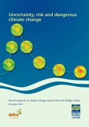
<strong>Scientific</strong> <strong>results</strong> <strong>from</strong> <strong>the</strong> <strong>Hadley</strong> <strong>Centre</strong>October 2002
In this reportThe ultimate objective of <strong>the</strong> UN framework convention on climate change(UNFCCC) is to stabilise atmospheric concentrations of greenhouse gases ‘at alevel that would prevent dangerous anthropogenic (human-induced) interferencewith <strong>the</strong> climate system’. In this report, we focus on some of <strong>the</strong> scientific issuesassociated with this aim, including <strong>the</strong> following. Physical commitment to climate changeEven if atmospheric greenhouse gas concentrations were stabilised immediately,we could still experience a changing climate and sea-level rise for more than1,000 years into <strong>the</strong> future due to past emissions. Fur<strong>the</strong>rmore, <strong>the</strong> greenhousegases we emit today and in <strong>the</strong> near future will initiate changes in climate thatwill be felt far into <strong>the</strong> future. Predictions of climate change when carbon dioxideconcentrations are stabilised in <strong>the</strong> futureReducing carbon dioxide (CO 2) emissions so that concentrations approachstabilisation will delay <strong>the</strong> amount of climate change we experience over <strong>the</strong>next 100 years and more. However, any realistic future stabilisation level is likelyto result in some damage. The effect of <strong>the</strong> carbon cycle on stabilisation ofatmospheric CO 2concentrationsWhen <strong>the</strong> feedbacks between <strong>the</strong> climate system and <strong>the</strong> carbon cycle are takeninto account, such as <strong>the</strong> increased emission of CO 2<strong>from</strong> soils as temperaturerises, <strong>the</strong> anthropogenic emissions consistent with a particular stabilisation levelof greenhouse gas concentrations are lower than previously thought.In addition, we include a short climate bulletin, highlighting recent observedchanges in climate.
IntroductionTen years since <strong>the</strong> Rio Earth SummitIn <strong>the</strong> 10 years since <strong>the</strong> Rio Earth Summit, ourunderstanding of <strong>the</strong> climate system — and <strong>the</strong> degree ofcertainty that mankind has already caused <strong>the</strong> climate towarm — have both increased. The Intergovernmental Panelon Climate Change (IPCC) now accepts that ‘<strong>the</strong>re is newand stronger evidence that most of <strong>the</strong> warming observedover <strong>the</strong> past 50 years is attributable to human activities’.The power of computers and our ability to simulate <strong>the</strong>climate system have also improved dramatically. Themodels we now use to make projections of future climateroutinely include <strong>the</strong> dynamics of <strong>the</strong> atmosphere and <strong>the</strong>ocean, and many physical processes, such as <strong>the</strong> effects ofclouds and <strong>the</strong> cooling effects of <strong>the</strong> atmospheric sulphurcycle. The most sophisticated simulations also includeatmospheric chemistry and <strong>the</strong> carbon cycle, and <strong>the</strong>irresponse to climate change.In <strong>the</strong> IPCC’s recent third assessment report, to which<strong>the</strong> <strong>Hadley</strong> <strong>Centre</strong> was a major contributor, <strong>the</strong> globalaverage temperature between 1990 and 2100 is projected torise by 1.4 °C to 5.8 °C, and <strong>the</strong> mean sea level is predictedto rise by 9 cm to 88 cm. At some locations, <strong>the</strong> increaseswill be larger than <strong>the</strong> global average, but at o<strong>the</strong>rs it willbe smaller. It is also becoming clear that extremes ofclimate, which are often responsible for most of <strong>the</strong>damage, are likely to change in <strong>the</strong> future.The <strong>Hadley</strong> <strong>Centre</strong>The Met Office’s <strong>Hadley</strong> <strong>Centre</strong> for Climate Prediction andResearch is charged by Government with undertakingresearch into climate change.The <strong>Hadley</strong> <strong>Centre</strong> provides a focal point in <strong>the</strong> UK for<strong>the</strong> scientific issues associated with climate change.Currently, <strong>the</strong> centre employs some 100 scientific andtechnical experts, and has access to two Cray T3Esupercomputers. It is supported by <strong>the</strong> Department forEnvironment, Food and Rural Affairs (DEFRA), o<strong>the</strong>rgovernment departments and <strong>the</strong> European Commision.The aims of <strong>the</strong> <strong>Hadley</strong> <strong>Centre</strong> are: to understand physical, chemical and biological processeswithin <strong>the</strong> climate system and develop state-of-<strong>the</strong>-artclimate models that represent <strong>the</strong>m; to use climate models to simulate global and regionalclimate variability and change over <strong>the</strong> past 100 years,and to predict changes over <strong>the</strong> next 100 years or more; to monitor global and national climate variabilityand change; to attribute recent changes in climate to specificfactors; and to understand <strong>the</strong> natural interannual-to-decadalvariability of climate, with <strong>the</strong> aim of forecasting it.In this report, we highlight areas of recent research thatdemonstrate <strong>the</strong> long timescales associated with climatechange and how <strong>the</strong> response of <strong>the</strong> climate to futureanthropogenic emissions may be strongly dependent onchanges in <strong>the</strong> biosphere.The current <strong>Hadley</strong> <strong>Centre</strong> building in Bracknell. In late 2003, <strong>the</strong>staff of <strong>the</strong> <strong>Hadley</strong> <strong>Centre</strong> will move, toge<strong>the</strong>r with <strong>the</strong> rest of <strong>the</strong>Met Office, to a new building in Exeter, in <strong>the</strong> south-west of England.Climate change science 1
Physical commitment to climate changeThe meaning of commitmentThe climate system has many different components and<strong>the</strong>se respond on different timescales. When increases ingreenhouse gas concentrations lead to an imbalancebetween <strong>the</strong> incoming visible energy <strong>from</strong> <strong>the</strong> sun andoutgoing energy <strong>from</strong> <strong>the</strong> earth, <strong>the</strong>re is net flow of heatinto <strong>the</strong> atmosphere. Gradually, <strong>the</strong> climate system warms;this increases <strong>the</strong> amount of energy leaving it until,eventually, a new balance occurs at a higher temperature.Although <strong>the</strong> atmosphere can respond relatively quickly tochanges in greenhouse-gas heating, <strong>the</strong> ocean and ice capsrespond more slowly. For instance, parts of <strong>the</strong> deep oceancan take more than 1,000 years to respond to a surfacegreenhouse warming. As a consequence, even if greenhousegas concentrations were stabilised immediately, <strong>the</strong> globaltemperature and sea level would continue to rise for aconsiderable amount of time into <strong>the</strong> future. This is <strong>the</strong>physical commitment to climate change.Global climate modelsTerrestrialradiationGreenhouse gases and aerosolSolarradiationCloudsPrecipitationAtmosphereTemperature change (°C)8642How do we calculate <strong>the</strong> physicalcommitment?In order to calculate <strong>the</strong> commitment to climate change,we estimated <strong>the</strong> response times of <strong>the</strong> climate system foratmospheric temperature changes, and <strong>the</strong> strength of thisresponse, using a 1,000-year simulation <strong>from</strong> <strong>the</strong> <strong>Hadley</strong><strong>Centre</strong>’s third-generation global climate model (see box).In this idealised model experiment, <strong>the</strong> carbon dioxideconcentrations were increased <strong>from</strong> pre-industrial levels tofour times pre-industrial levels over a period of 70 years,and <strong>the</strong>n held constant for <strong>the</strong> remainder of <strong>the</strong>experiment (below).TemperatureSea-level rise2.52.01.51.00.5Sea-level rise (m)Ice sheetssnowSea iceBiomassLandOcean00.0200 400Year600 800 1000Global climate models (often called general circulationmodels, or GCMs) simulate processes in <strong>the</strong> atmosphere,ocean and on <strong>the</strong> land. The atmospheric componentconsists of a three-dimensional representation of <strong>the</strong>atmosphere coupled to <strong>the</strong> land surface and cryosphere.The atmosphere model is similar to those used forwea<strong>the</strong>r forecasting but, because it has to produceprojections for decades or centuries ra<strong>the</strong>r than days, ituses a coarser level of detail. The ocean component of<strong>the</strong> models consists of a three-dimensional representationof <strong>the</strong> ocean and of sea ice. Global climate modelstypically have a horizontal resolution of a few hundredkilometres. Processes operating on smaller scales arerepresented through relationships with <strong>the</strong> larger scales.Climate models include <strong>the</strong> cooling effects ofsulphate aerosol particles. The most recent models alsoinclude aspects of <strong>the</strong> biosphere, carbon cycle andatmospheric chemistry.Simulated temperature change and <strong>the</strong> <strong>the</strong>rmal-expansioncomponent of sea-level rise for <strong>the</strong> four times pre-industrial CO 2concentration (4xCO 2) experiment. Global temperatures stabilisequicker than sea level, which is still rising after 1,000 years. Weestimate that it would take more than 2,500 years before <strong>the</strong> sealevel reaches 90% of its final value. The dashed line shows <strong>the</strong> yearwhen CO 2concentrations were stabilised.In order to estimate what would happen to temperaturein <strong>the</strong> real climate, if we were to stabilise concentrations ofgreenhouse gases, we combined <strong>the</strong> climate response timesand <strong>the</strong> strength of response <strong>from</strong> <strong>the</strong> 4xCO 2experimentwith observed increases in greenhouse gas concentrationover <strong>the</strong> past 150 years or so. The dashed line shows <strong>the</strong>year when CO 2concentrations were stabilised.Global climate models are used to simulate pastclimates and to predict future climates. They are alsoused to study natural variability and <strong>the</strong> physicalprocesses of <strong>the</strong> coupled climate system.2 Climate change science
Temperature change (°C)1.51.00.50.090° N45° N0° N45° SHow big is <strong>the</strong> current physical commitment?If we were able to stabilise greenhouse gas concentrationstoday <strong>the</strong>n we estimate that, by 2100, <strong>the</strong> temperaturewould rise by around 1.1 °C relative to pre-industrialtimes, and is predicted to rise to 1.6 °C eventually (below).2000 2200 2400 2600 2800YearThe rise in global mean temperature following stabilisation ofgreenhouse gas concentrations at present-day levels.We have estimated <strong>the</strong> regional commitment to climatechange by scaling <strong>the</strong> pattern of temperature rise <strong>from</strong> <strong>the</strong>4xCO 2simulation with our estimate of global meantemperature-rise commitment (below). The commitmentto temperature change will not be <strong>the</strong> same everywhereand, relative to pre-industrial times, some locations mayeventually warm by as much as 5 °C due to <strong>the</strong> increases ingreenhouse gas concentrations that have already occurred.90° S180° W 90° W 0° 90° E 180° E012Patterns of annual average temperature-rise commitment (°C) dueto anthropogenic emissions prior to present day.Lessons <strong>from</strong> <strong>the</strong> SRES emissions scenariosThe SRES emissions scenarios, published by <strong>the</strong> IPCC in2000, have formed <strong>the</strong> basis of many of <strong>the</strong> projections ofclimate change in <strong>the</strong> IPCC Third Assessment Report.They have very different pathways, with A1FI risingsharply <strong>from</strong> today’s value of 7 GtC of carbon emissionsup to a final value of about 30 GtC by 2100. At <strong>the</strong> o<strong>the</strong>r345extreme, <strong>the</strong> B1 scenario rises slowly to a peak of 9 GtC bymid-century and <strong>the</strong>n falls to below 5 GtC by 2100.When <strong>the</strong>se scenarios are used to drive <strong>the</strong> <strong>Hadley</strong><strong>Centre</strong> climate model, <strong>the</strong> resulting predictions (below)tell an interesting story. Until about 2040, <strong>the</strong> temperaturerise predicted for all four scenarios (A1FI, A2, B2, B1)follows very similar paths; <strong>the</strong> difference between <strong>the</strong>m ismainly due to natural variability.A1FIA2B1B22000 2020 2040 2060 2080 2100YearPredicted temperature change due to various SRES scenarios,expressed relative to present day.This similarity is partly because all four have built into<strong>the</strong>m <strong>the</strong> physical commitment to change due toemissions today and over past decades. In addition to this‘legacy’ effect, inertia in <strong>the</strong> climate system delays <strong>the</strong>response to <strong>the</strong> very different future emissions, and hence<strong>the</strong> effect of <strong>the</strong>se is not immediately apparent. By <strong>the</strong> endof <strong>the</strong> century, however, <strong>the</strong> warmings are very different:2 °C for B1 and 5 °C <strong>from</strong> A1FI emissions, expressedrelative to present day. This shows that <strong>the</strong> degree oflate-century warming is greatly influenced by levels ofemissions over <strong>the</strong> next few decades. In <strong>the</strong> case of <strong>the</strong>lowest (B1) emissions scenario, about one-quarter of <strong>the</strong>change during <strong>the</strong> 21st century is due to <strong>the</strong> physicalcommitment to emissions prior to today.ConclusionWe are already committed to a sizeable warming andsea-level rise. Fur<strong>the</strong>rmore, <strong>the</strong> increases in greenhousegas concentration caused by human emissions betweenpresent day and 2100 will <strong>the</strong>mselves lead to an additionallong-term warming and sea-level rise commitment farinto <strong>the</strong> future.6420Temperature anomaly (°C)Climate change science 3
Predictions of climate change when CO 2concentrationsare stabilised in <strong>the</strong> futureAnthropogenic CO 2 emisions (Gtc/yr)30252015105The emissions scenariosIn 1997, <strong>the</strong> Intergovernmental Panel on Climate Change(IPCC) suggested a number of emissions scenarios thatinclude reductions relative to <strong>the</strong> ‘business as usual’ case,and which ultimately stabilise atmospheric carbon dioxideconcentrations. We have examined <strong>the</strong> climate change forscenarios that stabilise CO 2concentrations at 750 parts permillion (ppm) and 550 ppm, about twice present-day andtwice pre-industrial levels, respectively. It is important tonote that, in <strong>the</strong> foreseeable future, stabilisation of CO 2concentrations is not <strong>the</strong> same as ei<strong>the</strong>r <strong>the</strong> stabilisation ofemissions, or of climate change. Fur<strong>the</strong>rmore, o<strong>the</strong>rgreenhouse gases have to be stabilised too.The profiles of anthropogenic emissions of CO 2whichcan achieve <strong>the</strong> IPCC stabilisation levels 1 (below, upperpanel) are very much less than <strong>the</strong> emissions for <strong>the</strong>‘business as usual’ scenario (IS92a) or <strong>the</strong> newer SRES A2scenario. The greenhouse gas concentrations (below,S550S750IS92aA1FI02000 2100 2200 2300B1lower panel) for <strong>the</strong> lowest of <strong>the</strong> SRES scenarios (B1) liesclose to or between <strong>the</strong> 550 ppm and 750 ppmconcentration curves for much of <strong>the</strong> 21st century.Predicting climate changeIn order to compare <strong>the</strong> climate change resulting <strong>from</strong> <strong>the</strong>550 ppm and 750 ppm stabilisation scenarios with <strong>the</strong>climate response to an unmitigated (IS92a) scenario, <strong>the</strong><strong>Hadley</strong> <strong>Centre</strong> climate model has been used to simulateeach of <strong>the</strong> three cases. Some of <strong>the</strong>se <strong>results</strong> were shownpreviously in <strong>the</strong> report published for CoP5.For simplicity, <strong>the</strong> climate model was driven with CO 2emissions only and did not explicitly include changes ino<strong>the</strong>r greenhouse gases or aerosols. The simulations herealso did not include <strong>the</strong> feedback between <strong>the</strong> carboncycle and climate change, but <strong>the</strong>se effects are discussedon pages 6 and 7.The climate change under CO 2stabilisation scenariosWith unmitigated emissions, temperatures by <strong>the</strong> 2080sare predicted to be about 3 °C above today’s (taken as <strong>the</strong>average over <strong>the</strong> period 1961–90). A global averagetemperature rise of 2 °C, which would occur by <strong>the</strong> 2050swith unmitigated emissions, will be delayed by about 50years under 750 ppm stabilisation, and by over 100 yearsunder 550 ppm stabilisation. By 2250, globaltemperatures will have risen to just over 2 °C abovetoday’s under <strong>the</strong> 550 ppm stabilisation scenario, and justover 3 °C under <strong>the</strong> 750 ppm scenario.The pattern of temperature change by <strong>the</strong> 2080s issimilar for all three emissions scenarios, with amagnitude roughly proportional to global temperature1050CO 2 concentration (ppm)950850750650550S550S750IS92aA1FIB143210Global temperature change (°C)4503502000 2100 2200 2300YearAnthropogenic CO 2emissions (top panel) and atmospheric CO 2concentrations (bottom panel).1900 2000 2100 2200YearThe global average temperature rise resulting <strong>from</strong> <strong>the</strong> unmitigatedemissions scenario (red), and emissions scenarios which stabiliseCO 2concentrations at 750 ppm (blue) and at 550 ppm (green).4 Climate change science
change. For both <strong>the</strong> stabilisation and unmitigatedscenarios, land areas will warm almost twice as fast asoceans, and winter high latitudes are also expected towarm more quickly than <strong>the</strong> global average, as areareas of nor<strong>the</strong>rn South America, India and sou<strong>the</strong>rnAfrica (below).The changes in precipitation (both positive and negative)by <strong>the</strong> 2080s are largest in <strong>the</strong> Tropics, but significantchanges do occur in mid- and high-latitude regions(below). The magnitude of changes is again smaller for <strong>the</strong>stabilisation scenarios than for <strong>the</strong> unmitigated scenarioand are roughly proportional to global temperature rise.90° N1.545° N90° S180° 90° W 0° 90° E 180°0°45° SPrecipitation change (mm/day)1.00.5IS92aS550S75090° N0.045° NPatterns of annual average temperature rise <strong>from</strong> <strong>the</strong> present dayto <strong>the</strong> 2080s, resulting <strong>from</strong> <strong>the</strong> unmitigated emissions scenario(top), an emissions scenario which stabilises CO 2at 750 ppm(middle) and one which stabilises at 550 ppm (bottom).45° S90° S180° 90° W 0° 90° E 180°90° S180° 90° W 0° 90° E 180°0 1 2 3 4 5 6 7Temperature rise (°C)1 There are an infinite number of pathways in which emissions can bereduced in order to stabilise concentrations in <strong>the</strong> atmosphere. The two mostwidely used are <strong>the</strong> IPCC ‘S’ scenarios and <strong>the</strong> ‘WRE’ scenarios. In <strong>the</strong> WREscenarios, <strong>the</strong> emissions deviate <strong>from</strong> a ‘business as usual’ scenario laterand peak at a higher level than in <strong>the</strong> IPCC cases.0°90° N45° N0°45° S-0.590° N 60° N 30° N 0° 30° S 60° S 90° SLatitudeZonally averaged annual mean precipitation changes (2080s minuspresent day) in IS92a, S750 and S550 scenarios.The changes in temperature and precipitation will haveimpacts on society across <strong>the</strong> globe. In some regions, <strong>the</strong>warmer temperatures and reduced precipitation will makewater scarce and <strong>the</strong> growing of crops more difficult. Ino<strong>the</strong>r areas, increases in precipitation (and <strong>the</strong> fraction ofprecipitation that falls in <strong>the</strong> most intense storm events)will contribute to more frequent flooding by rivers. At <strong>the</strong>coast, increases in sea level and changes in storminess willlead to inundation of unprotected land, more frequentflooding by storm surges and <strong>the</strong> loss of coastal wetlands.However, not all regions will be adversely affected.Increases in CO 2concentrations will enhance cropproduction in some locations, and increases inprecipitation will improve <strong>the</strong> situation in some regionswhere water is currently scarce.ConclusionMuch of <strong>the</strong> climate change and consequent impactsresulting <strong>from</strong> unmitigated emissions of CO 2will bedelayed by 50 to 100 years, if emissions scenarios leadingto stabilisation of CO 2are followed. In addition,stabilisation of CO 2at 550 ppm or less may even preventsome of <strong>the</strong> more serious impacts <strong>from</strong> occurring.Climate change science 5
The effect of <strong>the</strong> carbon cycle on stabilisation ofatmospheric CO 2concentrationsThe carbon cycleThe concentration of CO 2in <strong>the</strong> atmosphere depends on<strong>the</strong> amount emitted — for instance, <strong>from</strong> <strong>the</strong> burning offossil fuels and changes in land use — and <strong>the</strong> strength ofcarbon sinks, such as <strong>the</strong> ocean and biosphere, whichremove CO 2<strong>from</strong> <strong>the</strong> atmosphere.As <strong>the</strong> atmospheric concentration of CO 2increases, sodoes <strong>the</strong> ability of vegetation to take up CO 2<strong>from</strong> <strong>the</strong>atmosphere (<strong>the</strong> carbon fertilisation effect). However, <strong>the</strong>increases in CO 2lead to changes in temperature and rainfall,which can affect natural carbon sinks. Over land, climatechange can alter <strong>the</strong> geographical distribution of vegetationand hence its ability to store CO 2. In <strong>the</strong> <strong>Hadley</strong> <strong>Centre</strong>coupled climate–carbon cycle model, we find that climatechange <strong>results</strong> in a dying-back of <strong>the</strong> vegetation in nor<strong>the</strong>rnSouth America. Climate change also affects <strong>the</strong> amount ofCO 2emitted by bacteria in <strong>the</strong> soil. In <strong>the</strong> ocean, changes incirculation and mixing, which accompany climate change,alter <strong>the</strong> ocean’s ability to take up CO 2<strong>from</strong> <strong>the</strong> atmosphere.In addition, <strong>the</strong> warmer oceans absorb less CO 2.pathways that lead to stabilisation of atmospheric CO 2concentrations at a given level.IPCC technical note 3 discussed two alternative emissionspathways which would stabilise CO 2concentrations at aparticular level: <strong>the</strong> IPCC ‘S’ emissions, and <strong>the</strong> emissionsestimated by Wigley, Richels and Edmonds, <strong>the</strong> ‘WRE’emissions. These emissions were calculated using a simplecarbon cycle model that took account of <strong>the</strong> carbonfertilisation effect, but o<strong>the</strong>r feedbacks — such as thatassociated with <strong>the</strong> change of vegetation patterns or <strong>the</strong>oceans, due to climate change — were not included. Toinvestigate such effects we used a simple climate carbon-cyclemodel, which includes <strong>the</strong> feedbacks <strong>from</strong> vegetation, soilsand <strong>the</strong> ocean. This reproduces <strong>the</strong> <strong>results</strong> of <strong>the</strong> full <strong>Hadley</strong><strong>Centre</strong> coupled climate–carbon cycle model, and was usedto make new estimates of:(i) <strong>the</strong> emissions required to stabilise CO 2concentrationsat 550 ppm; and(ii) <strong>the</strong> concentrations resulting <strong>from</strong> <strong>the</strong> WRE emissionsscenarios.Veg andsoil carbonLand carbon cycle2000Without climate feedback (1929 GtC)With climate feedback (1194 GtC)Man-madeCO 2 emissionsLandsurfaceAtmosCO 2OceancarbonClimate modelCarbonflux andclimatechangeCarbonflux andclimatechangeCumulative CO 2 emissions (Gtc) <strong>from</strong> 185015001000500Ocean carbon cycleSchematic of a coupled climate–carbon cycle model. Green linesindicate carbon fluxes while red lines indicate physical changesand climate change.In order to include all of <strong>the</strong>se feedbacks, it is necessaryto treat <strong>the</strong> carbon cycle and vegetation as interactiveelements in full global climate modelling (GCM)experiments. This approach was pioneered by <strong>the</strong> <strong>Hadley</strong><strong>Centre</strong> and <strong>the</strong> first <strong>results</strong> were reported at CoP6.Stabilisation of CO 2concentrationat 550 ppmOn pages 4 and 5 of this report, CO 2emissions profilesthat can stabilise atmospheric concentrations of CO 2atspecific levels were discussed. We noted that, inprinciple, <strong>the</strong>re are an infinite number of emissions019002000 2100 2100 2300Cumulative emissions that are consistent with <strong>the</strong> WRE550 CO 2concentration scenario.The figure above shows two cumulative emissionsprofiles that eventually stabilise CO 2at 550 ppm. The blueline shows <strong>the</strong> result <strong>from</strong> <strong>the</strong> <strong>Hadley</strong> <strong>Centre</strong> modelwithout any carbon cycle feedbacks. The <strong>results</strong> are similarto <strong>the</strong> original WRE emissions scenario. The red line shows<strong>the</strong> result when <strong>the</strong> carbon cycle feedback is included. Thus,emissions may need to be reduced by much more thanoriginally thought to meet a specific concentration level.We can look at this result <strong>from</strong> <strong>the</strong> opposite direction,that is, by starting <strong>from</strong> <strong>the</strong> same emissions scenario(WRE550 in this case) and calculating <strong>the</strong> CO 2concentrations that would result. Without including <strong>the</strong>6 Climate change science
1000800feedbacks, <strong>the</strong> emissions eventually lead to stabilisation ofCO 2concentration at around 550 ppm, as intended(below). However, when <strong>the</strong> more comprehensive feedbacksare taken into account, <strong>the</strong> CO 2concentration rises muchhigher — to 780 ppm by 2300. Thus, <strong>the</strong> effect of carboncyclefeedbacks is to allow a greater fraction of CO 2emissions to remain in <strong>the</strong> atmosphere.With climate feedback Without climate feedbackCumulative CO2 emissions (GtC) 2000-23004000300020001000With climate changeWithout climate changeCO2 (ppm)6000400 600 800CO2 stabilisation level (ppm)Impact of carbon cycle feedbacks on stabilisation levels.10004002001900 2000 2100Year2200Impact of carbon cycle feedbacks on CO 2stabilisationconcentration for WRE550 emissions.Stabilisation at o<strong>the</strong>r concentration levelsStabilisation at o<strong>the</strong>r concentration levels has also beenconsidered. The figure (top, right) shows <strong>the</strong> relationshipbetween cumulative carbon emissions (<strong>from</strong> present day to2300) and <strong>the</strong> eventual stabilisation level. The blue lineshows how much <strong>the</strong> cumulative emissions would need tobe in order to stabilise CO 2at different levels. However,when <strong>the</strong> carbon cycle feedbacks are included, <strong>the</strong>‘allowable’ emissions are greatly reduced for allstabilisation concentration levels (red line). For example, ifwe chose to stabilise at 750 ppm, <strong>the</strong> estimate ofcumulative emissions is around 2,500 GtC when <strong>the</strong>feedback is not included but, with carbon cycle andvegetation feedbacks, only 1,400 GtC would be required.Change in <strong>the</strong> storage of carbon on landIn order to show how <strong>the</strong> storage of carbon on land (invegetation and <strong>the</strong> soil) changes in <strong>the</strong> future in <strong>the</strong><strong>Hadley</strong> <strong>Centre</strong> model with interactive carbon cycle andvegetation, <strong>the</strong> change in land carbon between present dayand 2100 has been estimated for different regions for <strong>the</strong>550 ppm stabilisation scenario and, for comparison, anunmitigated (IS92a) scenario.Globally, <strong>the</strong> land carbon store increases by almost 50 GtCover <strong>the</strong> century when emissions follow a stabilisationpathway, because both soil-carbon and vegetation-carbonstores increase. But, when emissions continue on anunmitigated course, <strong>the</strong> carbon store decreases by about170 GtC. This is because increased soil respiration, and adie-back of vegetation in South America, toge<strong>the</strong>r exceed<strong>the</strong> increases in vegetation storage in o<strong>the</strong>r regions(below). Note that <strong>the</strong> change in <strong>the</strong> natural terrestrialcarbon cycle <strong>from</strong> a sink to a source by <strong>the</strong> end of <strong>the</strong>century with unmitigated emissions means that, insteadof <strong>the</strong> current situation where it offsets man-madeemissions, in future it could amplify <strong>the</strong> contribution<strong>from</strong> human activities.80.060.040.020.00.0-20.0-40.0-60.0-80.0-100.0-120.0-140.0ConclusionN. America24.1AfricaAustralia14.1S. America8.111.1-55.7-8.1-14.0-30.7-127.0550 stabilisationUnmitigatedEurasia54.4Change in land carbon storage with climate carbon cycle feedbacks between2000 and 2100.Preliminary calculations show that including <strong>the</strong>feedbacks between climate change and <strong>the</strong> carbon cyclegreatly reduces <strong>the</strong> ‘allowable’ emissions that lead to CO 2concentration stabilisation at a given level. It does this byreducing <strong>the</strong> strength of carbon dioxide sinks.Climate change science 7
Climate Bulletin 20020.8The global mean surface temperature in 2001 wasapproximately 0.63 °C above <strong>the</strong> average for <strong>the</strong> late 19thcentury. Despite <strong>the</strong> mitigating influence of <strong>the</strong> La Niñacool event in <strong>the</strong> eastern and central tropical Pacific forpart of <strong>the</strong> year, it was <strong>the</strong> second warmest year on record.The 10 warmest years have all occurred since 1983, wi<strong>the</strong>ight of <strong>the</strong>m since 1990.The year 2002 has continued this warming trend,with <strong>the</strong> first six months of <strong>the</strong> year being <strong>the</strong> warmeston record in <strong>the</strong> nor<strong>the</strong>rn hemisphere and <strong>the</strong> secondwarmest globally.Difference (°C) <strong>from</strong> 1961–903.02.52.01.51.00.50.0-0.5-1.0-1.5-2.0-2.5-3.01880 1900 1920 1940 1960 1980 2000Temperature difference (°C)0.60.40.20.0–0.2Equatorial Pacific sea-surface temperatures (°C) relative to 1961–90,for 1871 to August 2002.Extremes of temperature have also changed in recenttimes. Using a data set collected during <strong>the</strong> 45 years <strong>from</strong>1950 to 1995, it appears, for instance, that <strong>the</strong>re has been asignificant reduction in <strong>the</strong> number of frost days over mostof <strong>the</strong> nor<strong>the</strong>rn hemisphere mid-latitude land mass. Themost notable exception is an increase over Iceland (below).–0.490° N1860 1880 1900 1920 1940 1960 1980 2000Annual combined land-surface air and sea-surface temperatureanomalies (°C) for <strong>the</strong> period 1860 to June 2002. The anomaly for2002 is based on <strong>the</strong> average anomalies between January and June.90° N60° N30° N0°30° S45° N180° W 90° W 0° 90° E 180° E0°45° S-6 -4 -2 0 24Change over a decade in <strong>the</strong> observed number of frost days peryear, estimated <strong>from</strong> <strong>the</strong> 1950–95 data set. Black lines encloseregions where trends are significant at <strong>the</strong> 5% level.90° S120° W 60° W 0° 60° E 120° E 180° E-3 -2 -1 0123Surface temperature anomalies (°C) relative to 1961–90 for <strong>the</strong>six-month period January to June 2002.Global average temperatures tend to be elevated duringlarge El Niño events and lowered during La Niñas. ElNiños — and <strong>the</strong> large circulation changes associatedwith <strong>the</strong>m — also affect o<strong>the</strong>r climate variables, such asrainfall, over a very wide area. The warmest full year onrecord, 1998, coincided with <strong>the</strong> most recent large El Niño.Measurements of surface temperature patterns show thatwe have recently entered a new El Niño phase, but it is notyet clear how large this event will be (top right).8 Climate change science
Staff at <strong>the</strong> Met Office’s <strong>Hadley</strong> <strong>Centre</strong>:September 2002Lisa Alexander, Richard Allan, Rob Allan, Tara Ansell,David Baker, Helene Banks, David Barnett, Martin Best,Richard Betts, Penny Boorman, Philip Brohan, SimonBrown, Cyndy Bunton, Erasmo Buonomo, AndrewBushell, John Caesar, Mick Carter, Peter Cox, MichelCrucifix, Stephen Cusack, Paul Davison, AnthonyDickinson, Buwen Dong, Chris Durman, Ian Edmond,John Edwards, Chris Folland, Nicola Gedney, Pip Gilbert,Margaret Gordon, Alan Grant, Jonathan Gregory, DaveGriggs, Mark Hackett, Jen Hardwick, Mike Harrison, DavidHassell, Diane Hatcher, Ros Hatcher, David Hein, ChrisHewitt, Emma Hibling, Tim Hinton, Briony Horton,William Ingram, Sarah Irons, Geoff Jenkins, Tim Johns,Colin Johnson, Andy Jones, Chris Jones, Gareth Jones,Richard Jones, Kumar Kaushal, Ann Keen, Roy Kershaw,John King, Jeff Knight, Joe Lavery, Evelyn Leung, EllenLewis, Spencer Liddicoat, Linda Livingston, Jason Lowe,Gordon Lupton, Gill Martin, Kathy Maskell, MarkMcCarthy, Ruth McDonald, Alison McLaren, JohnMitchell, Steve Mullerworth, James Murphy, AmoonOsman, Elisabeth Öström, Alison Pamment, AnnePardaens, David Parker, Vicky Pope, Nick Rayner, GrahamRickard, Jeff Ridley, Mark Ringer, David Roberts, MalcolmRoberts, Jose Rodriguez, Mark Rodwell, Bill Roseblade,Dave Rowell, Maria Russo, Yvonne Searl, Cath Senior,David Sexton, John Siddorn, Doug Smith, Steve Spall,Peter Stott, Rachel Stratton, Yong Ming Tang, Simon Tett,Jean-Claude Thelen, Robert Thorpe, Thomas Toniazzo,Paul Van der Linden, Michal Vanicek, Michael Vellinga,Mark Webb, Paul Whitfield, Keith Williams, AlastairWilliams, Damian Wilson, Simon Wilson, Richard Wood,Margaret Woodage, Stephanie Woodward, Peili WuThis report is also available at:www.metoffice.com/research/hadleycentre/pubs/brochures/B2002/global.pdf
Met Office <strong>Hadley</strong> <strong>Centre</strong> London Road Bracknell Berkshire RG12 2SY United KingdomTel: +44 (0)1344 855680 Fax: +44 (0)1344 854898E-mail: hadley@metoffice.com www.metoffice.comDesigned and produced by <strong>the</strong> Met Office © Crown copyright 2002 02/0596 Met Office and <strong>the</strong> Met Office logo are registered trademarks