Visual SLAM Based on Rigid-Body 3D Landmarks - Computer vision ...

J Intell Robot Syst (2012) 66:125–149DOI 10.1007/s10846-011-9601-5<strong>Visual</strong> <strong>SLAM</strong> <strong>Based</strong> on Rigid-Body 3D LandmarksPatricio Loncomilla · Javier Ruiz del SolarReceived: 17 December 2010 / Accepted: 11 May 2011 / Published online: 17 August 2011© Springer Science+Business Media B.V. 2011Abstract In current visual <strong>SLAM</strong> methods, pointlikelandmarks (As in Filliat and Meyer (CognSyst Res 4(4):243–282, 2003), we use this expressionto denote a landmark generated by a pointor an object considered as punctual.) are usedfor representation on maps. As the observationof each point-like landmark gives only angularinformation about a bearing camera, a covariancematrix between point-like landmarks must be estimatedin order to converge with a global scaleestimation. However, as the computational complexityof covariance matrices scales in a quadraticway with the number of landmarks, the maximumnumber of landmarks that is possible touse is normally limited to a few hundred. In thispaper, a visual <strong>SLAM</strong> system based on the useof what are called rigid-body 3D landmarks isproposed. A rigid-body 3D landmark representsthe 6D pose of a rigid body in space (positionand orientation), and its observation gives fullposeinformation about a bearing camera. Eachrigid-body 3D landmark is created from a set of Npoint-like landmarks by collapsing 3N state componentsinto seven state components plus a set ofparameters that describe the shape of the landmark.Rigid-body 3D landmarks are representedand estimated using so-called point-quaternions,which are introduced here. By using rigid-body3D landmarks, the computational time of anEKF-<strong>SLAM</strong> system can be reduced up to 5.5%, asthe number of landmarks increases. The proposedvisual <strong>SLAM</strong> system is validated in simulated andreal video sequences (outdoor). The proposedmethodology can be extended to any <strong>SLAM</strong> systembased on the use of point-like landmarks,including those generated by laser measurement.Keywords Robotics · Localization · <strong>SLAM</strong> ·6D <strong>SLAM</strong> · <strong>Visual</strong> <strong>SLAM</strong> · Mono<strong>SLAM</strong> ·3D Mapping · Model reduction1 IntroductionP. Loncomilla · J. R. del SolarDepartment of Electrical Engineering,Universidad de Chile, Santiago, ChileP. Loncomilla (B) · J. R. del SolarAdvanced Mining Technology Center,Universidad de Chile, Santiago, Chilee-mail: ploncomi@ing.uchileSimultaneous Localization and Mapping (<strong>SLAM</strong>)has been one of the most highly investigated topicsin mobile robotics in the last 20 years. Severalworkshops, special sessions in conferences andspecial issues in journals have been devoted tothis research topic. Vision-based or visual <strong>SLAM</strong>,i.e. the attempt to solve <strong>SLAM</strong> using standard

126 J Intell Robot Syst (2012) 66:125–149cameras as the main sensory input [2], has attractedthe attention of the <strong>SLAM</strong> communityin recent years. Main challenges in vision-based<strong>SLAM</strong> are robust feature detection, efficient androbust data association and loop-closure, andcomputationally efficient large-scale state estimation[2]. <strong>Visual</strong>-landmark definition, representation,and estimation are some of the key issues totackle in order to address these challenges.In the current vision-based <strong>SLAM</strong> literature,points are selected as landmarks because of theirdirect geometrical interpretation, which enablesthe straightforward formulation of the <strong>SLAM</strong>problem [3–5]. However, when a fully calibratedcamera observes a point, only weak angular informationthat relates the observation to the posesof the landmarks and the camera is obtained.As only angular information is available, severalpossible maps can explain the observations, sinceany rotation, translation or scale transformationsapplied to them preserve the coherence betweenthe model and the measurements [3].As each point-like observation fulfills only 2degrees of freedom, and the map has 7 degreesof freedom, sets of several simultaneously observedpoints must be used in order to estimatethe map, which necessitates the use of a fullcovariancematrix [6]. When the size of the mapincreases, the number of landmarks becomes veryrelevant, as the number of computations requiredto update the covariance matrix is proportionalto the square of the full state size. As a result ofthis fact, the map size is limited by the numberof landmarks, which can increase only up to afew hundred for real-time applications. Since amap created by using only angular information isweakly constrained, robustness and precision oflocal maps become very limited [3]. Landmarkrecognition is based on point-projection predictionand matching of local patches around eachpoint, which gives weak association information,forcing the use of RANSAC-like strategies fordiscarding sets of false associations [4]. Then, alternativelandmark-modeling methodologies arerequired in order to overcome the inherent limitationsof point-like landmarks.Landmarks, in their widest sense, are geometricalfeatures that enable the description of amap in a fashion understandable to humans, andthat make possible self-localization. By followingthis wide definition, it can be noted that humanslocalize themselves using landmarks that do notcorrespond to points, but instead correspond towide regions in space that are recognized by visualinspection, by means of a hierarchy of increasinglysophisticated representations. <strong>Visual</strong> observationsfrom these wide-region landmarks are not limitedto angular information, since they include bothrelative distance and orientation between the observerand each landmark. In addition, humansare able to give descriptions of places or pathsbetween different places by using references tosemantic information that is more related to fullobjects than to points. Thus, the ability of a robotto use landmarks related to wide areas, instead ofto points, is desirable in order to generate morerobust observations, to facilitate semantic labeling,and to reduce the amount of data needed tomaintain the map.In order to address the previously mentionedaspects, a methodology for generating, representingand estimating rigid-body 3D landmarks isproposed. A rigid-body 3D landmark representsthe 6D pose of a rigid body in space (position andorientation), and its observation gives full-poseinformation about the camera. Each rigid-body3D landmark is created from a set of N pointlikelandmarks by collapsing 3N state componentsinto seven state components plus a set of parametersthat describe the shape of the landmark (socalledbody points and their covariance matrices).Rigid-body 3D landmarks are represented andestimated using point-quaternions, which are hereintroduced and named.A visual <strong>SLAM</strong> system that uses point-likeand rigid-body 3D landmarks, based on the EKF-<strong>SLAM</strong> formulation, is also proposed. The use ofrigid-body 3D landmarks permits reducing thecomputational time of the EKF-<strong>SLAM</strong> system upto 5.5%, as the number of landmarks increases.The proposed visual <strong>SLAM</strong> system is validated insimulated and real video sequences.This paper is organized as follows. Importantrelated work is presented in Section 2. InSection 3, the proposed methodology used torepresent and estimate rigid-body 3D landmarksis described. In Section 4, the proposed visual<strong>SLAM</strong> system is explained. An experimental

J Intell Robot Syst (2012) 66:125–149 127evaluation of the system is presented in Section 5.Finally, some conclusions of this work are drawnin Section 6.2 Related WorkVision-based <strong>SLAM</strong> is an important researchtopic that has attracted increasing attention inthe mobile robotics community. Interestingly, assmart-phones and digital cameras are gaining popularity,vision-based <strong>SLAM</strong> has acquired manypotential applications beyond robotics, “due tothe capability it can give a camera to serve as ageneral-purpose 3D position sensor” [2].Most of the current work related to monocularbasedvisual localization stands on two approaches:structure-from-motion recovery, andmonocular <strong>SLAM</strong>. Structure-from-motion recoveryis based on algorithms that estimate correspondingpoints between consecutive imageswithout using a dynamic model. Methodologiesbased on Nistér’s visual odometry [7] using optimalpreemptive RANSAC [8] applied over setsof three- and five-points, which are extracted byHarris filtering and processed using local bundleadjustment optimization, can achieve impressiveresults over large paths, but they accumulate anever-increasing error over time, as they are basedonly on relative motion.Monocular visual <strong>SLAM</strong> approaches, based onthe seminal works of Davison [6, 9], can achieveimpressive results in small to middle-size maps,but the management of large maps is a hardtopic to face because of scale drifts, covariancematrix expansion, and loop-closure limitations.Live dense reconstruction [10] can be achievedby updating an active mesh by means of constrainedoptical-flow based minimization. Scalableactive matching [5] has been proposed to managelarge maps that involve a large amount ofcross-correlation by using a graph-pruning approachin order to reduce covariance data, andto limit uncertainty propagation between distantpoints. A drift-aware monocular <strong>SLAM</strong> [3]has been proposed to model scale-drift by usinga Lie group approach over the rotationtranslation-scaletransformation group, to achievedifferential-constrained bundle-adjustment optimizationfor loop closing. As the time neededfor RANSAC to solve a problem increases dramaticallywith the number of points needed forconforming a minimal subset, 1-point RANSAC[4] has been proposed to achieve fast data association.This approach is based on using 1 pointto update the pose of the robot, and then usingthe new robot’s pose for evaluating consensus onthe other points using a chi-square test. Finally,appearance and 3D geometry [11] have been usedto cluster a map into sets of points that are closein space, and that have similar image areas aroundthem. This approach looks promising for buildingsemantic models.As has been already mentioned, some of thecurrent problems of visual <strong>SLAM</strong> systems arederived from the fact that the perception of apoint-like landmark does not allow the camera’spose to be inferred, and several points must beperceived and analyzed. To overcome this drawback,high-level landmarks based on sets of pointsscattered over the object surfaces can be used[12, 13]. In [12] high-level structures, such asplanes and lines, are built online using a bottomupprocess that first maps point-like and line-likelandmarks, and then searches for sets of themthat agree with the high level landmarks’ hypothesis.In [13] locally planar landmarks representedusing the inverse depth parametrization [14] aredefined. The camera’s state, landmark’s normalplane,and measurement errors are representedas Lie groups. Local reference frames defined bya central point and Euler-like angles have beenused in 3D laser <strong>SLAM</strong> for representing localplanar patches, which generate more compact andmeaningfully maps [15–18]. However, the use ofplane-based features limits the ability of the methodsto handle general outdoor environments, andobservations related to planes lose two degrees offreedom respect to full pose information, whichlimits the amount of information gathered fromeach observation. The approach proposed in thiswork is also based on the collapsing of pointlikelandmarks into high-level landmarks, but themain differences are the use of non-planar 3Dlandmarks, which adds flexibility to the system,and the definition of a methodology for landmarkrepresentation and estimation that is basedon the use of point-quaternions, which form a

128 J Intell Robot Syst (2012) 66:125–149rotationally-symmetric algebraic group representationfor poses in space.3 Rigid-Body 3D Landmark Representationand EstimationA rigid-body 3D landmark, from now on referredto as a 3D landmark, represents the 6D pose ofa rigid body in space. A rigid body is composedby a set of observable points called body points,which are used to create a 3D landmark. The poseof the 3D landmark is determined by the locationof the rigid body points when referred to a globalreference frame. The pose of the 3D landmarkis encoded by using a point and a quaternion[19] chained into a unique object named a pointquaternion.The covariance of a 3D landmark’spose is determined by the covariance of its associatedpoint-quaternion.In a <strong>SLAM</strong> system, every time a subset of thebody points is observed, a compatible pose for the3D landmark is computed and used as a virtualobservation. Uncertainty related to the observationof the body points can be propagated intouncertainty in the pose of the 3D landmark. Thevirtual observation and its covariance enable thecorrection of the 3D landmark pose estimation.3.1 6D pose representation usingpoint-quaternionsA point-quaternion η is introduced in this paperas a 7D mathematical object that is composed bya point t and a quaternion q. The point is usedto denote a position, and the quaternion is usedto denote an orientation. In this way, a pointquaternioncan represent a 6D pose in space. Aquaternion can be formed by specifying a unitaryrotation axis ω, and a rotation angle θ. Then, η isdefined as:η 7×1 =(t3×1q 4×1); q =⎛ ⎞ ⎛⎞a cos (θ/2)⎜ b⎟⎝ c ⎠ = ⎜ ω X sin (θ/2)⎟⎝ ω Y sin (θ/2) ⎠ ;d ω Z sin (θ/2)⎛ ⎞xt = ⎝ y ⎠ (1)zSimilarly as in the case of using transformationmatrices, using point-quaternions allows defininga transformation operation, transop, over a vectorp, consisting of a rotation followed by atranslation:transop (η, p) = q · p · q −1 + t (2)The inverse transformation, inv_transop, isdefinedas:inv_transop (η, p) = q −1 · (p − t) · q (3)Point-quaternions can be composed by using amultiplication operation, which is defined as:η 1 · η 2 =( ) ( ) (t1 t2 q1 · t· = 2 · q −1 )1+ t 1q 1 q 2 q 1 · q 2(4)Point-quaternions containing a zero quaternionare ill-posed as they do not represent any rotation.Valid point-quaternions and their multiplicationform a group as they have closure, associativity,an identity element (η I ) and an inverse element(see proof in [20]):η I =η −1 =(03×1) ( 0, 0, 0T=1( )−q−1 · t · qq −11, 0, 0, 0 T ),(5)A special sum for point-quaternions is notdefined because of the lack of distributive properties,but vector summation can be applied forJacobian-calculation purposes [20].Point-quaternion multiplication can be usedto relate different reference systems as transformationmatrices do. Coordinates from points ona reference system A can be transformed intocoordinates on a reference system B by usinga point-quaternion η AB . Coordinate transformationsbetween reference systems A, B and C canbe composed by using point-quaternion multiplication(the multiplication direction is the same asthat used in homogeneous matrix composition):η AC = η BC · η AB (6)

J Intell Robot Syst (2012) 66:125–149 129Each point-quaternion η has an associated homogeneousmatrix H(η) that represents the sametransformation:(( )) tH (η) = Hq⎛=⎜⎝a 2 +b 2 −c 2 −d 2a 2 +b 2 +c 2 +d 22bc−ada 2 +b 2 +c 2 +d 22bc+2ad a 2 −b 2 +c 2 −d 2a 2 +b 2 +c 2 +d 2 a 2 +b 2 +c 2 +d 22bd−2aca 2 +b 2 +c 2 +d 22bd+2aca 2 +b 2 +c 2 +d 22cd−2aba 2 +b 2 +c 2 +d 22cd+2ab a 2 −b 2 −c 2 +d 2a 2 +b 2 +c 2 +d 2 a 2 +b 2 +c 2 +d 2t Xt Yt Z0 0 0 1⎞⎟⎠(7)Thus, point-quaternions can be used for thesame purposes as homogeneous matrices, beingmore compact and well-posed as they do notinclude distorting effects associated with homogeneousmatrices. As each homogeneous matrixcontains 12 variable components, the errorcovariance representation associated with a homogeneousmatrix uses 12 × 12 components,and it is ill-posed when representing pose uncertaintyas it can encode uncertainty about axisorthogonality and scaling. Conversely, the covariancematrix of a point-quaternion, a 7 × 7symmetric semipositive-definite matrix, encodesthe uncertainty about a pose in space, and itis well posed as it always represents pure poseuncertainties.3.2 Rigid-body 3D Landmark GenerationProcedureThe procedure used for creating a rigid-body 3Dlandmark from N individual point-like landmarks(points) involves transforming 3N position statecomponents into seven-pose state components.The covariance representation must be transformedat the same time.First, the <strong>SLAM</strong> state vector x (see Section 4)is divided into the set of points p SET to be fused,and the other state components o:x =(pSETo⎛); p SET = ⎝⎞ ⎛ ⎞p 1x i... ⎠ ; p i = ⎝ y i⎠ (8)p N z iBody points i are computed by subtractingthe mean position value from each point p i to befused: i = p i − m, i = 1,...,N;m 1 NN∑p i (9)In general terms, a point-quaternion defining acoordinate transformation T that relates a set ofpoints in a reference frame A to a set of points in areference frame B, can be computed with minimalerror as:T(p (B)1,...,p (B)= arg minη LNN), p(A) 1,...,p (A)N(∑ N ∥∥q LN · p (A)i=1−p (B)iii=1· q −1LN + t LN∥ 2) (10)Given that the transformation that relates thebody points to the original points corresponds toa translation m and an identity rotation:η LAND−MAP =( )tLAND−MAPq LAND−MAP= T (p 1 ,...,p N , 1 ,..., N )( ) m=1(11)The new state representation of the 3D landmarkis put into the full state vector:x NEW =(ηLAND−MAPo)(12)The covariance matrix of the state P is dividedinto four sub matrices, where P pp contains thecovariances from the points to be fused:( )Ppp PP =po,P op P oo⎛P pp = ⎜⎝P (1,1)3×3P (1,2)3×3... P(1,N)3×3P (2,1)3×3P (2,2)3×3... ...... ... ... ...P (N,1)3×3... ... P (N,N)3×3⎞⎟⎠(13)

130 J Intell Robot Syst (2012) 66:125–149Considering the size reduction of the vectorstate, P will adopt the following form:( )P77 PP =7o(14)P o7 P ooBy considering that each body point i willhave an associated covariance P (i) , covariancepropagation from p i and i into η LAND−MAP canbe estimated using a first order Taylor expansion:⎛P (1) ⎞P 77 = J p P pp J T p − J ⎝ ... ⎠ JP (N) T (15)withJ p = ∂T (p 1,...,p N , 1 ,..., N );∂ (p 1 ,...,p N )J = ∂T (p 1,...,p N , 1 ,..., N )∂ ( 1 ,..., N )P 7o and P o7 are updated as:=−J p (16)P 7o = J p P po ; P o7 = P op J T p (17)The error associated to P pp must be dividedinto the P 77 pose covariance and the P (i)body-points covariance. The decomposition isnot unique as any choice for the set of covariancesP (i) and P 77 is valid, when all of theinvolved covariance matrices are positive semidefinite.Then, several criteria for selecting theP (i) can be generated. In this work, two criteriawill be considered, maximal pose covariance andmaximal body-points covariance.1. Maximal pose covariance. The procedure considersthe following steps. First, transfer allthe covariance error associated to P pp intoP 77 :P 77 = J p P pp J T p (18)Then, compute the covariance matrix P REC ,which corresponds to an approximation ofP 77 :P REC = GP 77 G T (19)withG = ∂U ( 1,..., N ,η LAND−MAP )∂ ( 1 ,..., N )and(20)⎛q LAND−MAP · 1 · q −1LAND−MAP + t ⎞ ⎛ ⎞LAND−MAP p 1U ( 1 ,..., N ,η LAND−MAP ) = ⎝...⎠ ≈ ⎝ ... ⎠ (21)q LAND−MAP · N · q −1LAND−MAP + t LAND−MAP p NAfterwards, calculate the covariance matrixof each body point P (i) by subtracting theoriginal P pp and its approximation P RECas:P (i) = D(i,i) 3×3(22)P DIFF = P pp − P REC⎛= ⎜⎝D (1,1)3×3D (1,2)3×3... D(1,N)3×3D (2,1)3×3D (2,2)3×3... ...... ... ... ...D (N,1)3×3... ... D (N,N)3×3⎞⎟⎠(23)Finally, each P (i) must be checked for positivesemidefiniteness by making zero its negativeeigenvalues and reconstructing the matrix.2. Maximal body-points covariance. Transfer themaximal amount of covariance to the set ofbody points P (i) by minimizing the amountof covariance that is transferred to P 77(the Levenberg-Marquardt optimization procedureis used):{ ( (min λ LOWER P pp −α 1α 1 ,α 2withD = diag ( P pp)P (1,1)3x3...P (N,N)3x3) )} 2− α 2 D(24)(25)and λ LOWER (M) the lower eigenvalue of acertain matrix M.

J Intell Robot Syst (2012) 66:125–149 131As any covariance matrix must be positivesemidefinite, it is minimal when its lowereigenvalue is near to zero. After α 1 and α 2 aredetermined, the P (i) are updated as:⎛⎞⎞⎝P (i)...P (N)⎛⎠ = α 1⎝P (1,1)3×3...P (N,N)3×3⎠+ α 2 D (26)Then, P 77 is computed using (15).The body points and their covariance matricesare stored in a special data structure, whichdoes not need to be updated by the <strong>SLAM</strong>update procedure.3.3 Rigid-body 3D Landmark GenerationCriterionThe decision for generating a new rigid-body 3Dlandmark depends on the covariance of the pointsto be fused. Small covariances indicate smallererrors in the observations. Positive and similarcross-covariances between the points assure thatthe correction of one point generates a similarcorrection in all the other points, and then theybehave as a rigid body.The proposed fusion criterion is fast to computeand enables the creation of sets of landmarks thatare candidates for fusing. It is based on the analysisof the covariance matrix of the points to befused. A variability index (varIndex) is computed.It indicates the degree of variation of the componentsfrom a subset of the covariance matrix.Subsets with low variability indicate that crosscovariances are similar.Before computing the variability indices of thecovariance matrix P pp , their diagonal componentsP i = P (i,i)3×3(see Eq. 13) are ordered by decreasingtrace-value of the covariance sub matrices foreach point:P i > P j ⇒ P iXX + P iYY + P iZZ> P jXX + P jYY + P jZ Z (27)with⎛⎞P iXX P iXY P iXZP i = ⎝ P iY X P iYY P iY Z⎠ (28)P iZX P iZY P iZZTheorderingindicatedin(27) can be alteredfor eliminating terms that have several negativecross-covariances over the X, Y or Z components(see details in [20]). The variability index is computedon several windows in the covariance matrixusing summed area tables for computing fastaverage values into the window:varIndex = min C X (q, r, q + M, r + M)q,r+ C Y (q, r, q + M, r + M)with+ C Z (q, r, q + M, r + M) (29)∑q 1PqrX 2 Xq=q 0 r=r 0C X (q 0 , r 0 , q 1 , r 1 ) =(q 1 − q 0 + 1)(r 1 − r 0 + 1)⎛q 1⎞∑ ∑r 1 P qrX Xq=q 0 r=r 0 × ⎜⎟⎝(q 1 −q 0 +1)(r 1 −r 0 +1) ⎠∑q 1C Y (q 0 , r 0 , q 1 , r 1 ) =(q 1 − q 0 + 1)(r 1 − r 0 + 1)⎛q 1⎞∑ ∑r 1 P qrYYq=q 0 r=r 0 × ⎜⎟⎝(q 1 −q 0 +1)(r 1 −r 0 +1) ⎠r 1 ∑r 1 ∑PqrYY2 q=q 0 r=r 0∑q 1PqrZ 2 Zq=q 0 r=r 02(30)2(31)C Z (q 0 , r 0 , q 1 , r 1 ) =(q 1 − q 0 + 1)(r 1 − r 0 + 1)⎛q 1⎞∑ ∑r 1 P qrZ Zq=q 0 r=r 0 × ⎜⎟⎝(q 1 − q 0 + 1)(r 1 −r 0 +1) ⎠r 1 ∑2(32)and M the number of points to be grouped (e.g.M = 10).

132 J Intell Robot Syst (2012) 66:125–149Finally, when a window has a varIndex below athreshold th, the selected points are collapsed intoa 3D landmark using the procedure described inSection 3.2.3.4 Virtual and Estimated 3D ObservationsEvery time the rigid body represented by therigid-body 3D landmark is observed, measurementsinvolving the body points are obtained. Inthis work, body points are detected as points ofinterest using the SURF methodology [21]. Theposition of each interest point (pos x , pos y ) istranslated into normalized pixel coordinates, anddefines a basic observation z uv to be used by the<strong>SLAM</strong> system:z uv =(ux)=v y( )posx /distFoc xpos y /distFoc y(33)with distFoc X /distFoc Y the focal distances in xand y, respectively.After data association (see description inSection 4.2), the set of measurements in normalizedcoordinates {z uv } can be transformed into avirtual observation of a rigid-body 3D landmarkz rb3D . This requires minimizing a measurementerror that relates the coordinates of the bodypoints, the pose of the corresponding rigid-body3D landmark (whose identity is determined in thedata association process), and the real measuredobservations. As the virtual observation computationinvolves minimizing an error, an initial posemust be provided for the minimization algorithm.The initial pose is estimated by using the threepointalgorithm [22] in several random-selectedtriplets of measured interest points. The threepointalgorithm (alg3p function) enables the calculationof the positions of three points in spacewhen the projected points and the distances betweenthe points in space are known. As up tofour solutions can be obtained, a fourth point isneeded for disambiguation. Twelve sets of fourpoints are used to generate a set of candidateposes. The last detected pose is also added to thisset. The candidate pose with the lowest error isselected. By using this procedure, an initial poseη 0 that projects a triplet of body points into threemeasured interest points on the image with lowerror is obtained:η 0 = arg minη abcd ∈I (E P (η abcd )) ; I = {η 1 ,,,η 13 } (34)with(( )uaη abcd = alg3p a , b , c , d , ,v aandi=1(ucv c),(ubv b),(udv d))a ̸= b ̸= c ̸= d (35)E P (η LC )N∑=∥ projection ( ( )∥q LC · i · q −1LC + t ) ui ∥∥∥LC −v i(36)The projection operation maps points in spaceinto the image space:( ) u=v( ) x/zy/z⎛ ⎞x= projection ⎝ y ⎠ (37)zThen, the virtual observation z rb3D is computedby iterative optimization using Levenberg-Marquardt, using as the initial solution η 0 :z rb3D = V (u 1 ,v 1 ,...,u N ,v N , 1 ,..., N )= η LAND−CAM−MEASURED= arg minη iE P (η i ) (38)The error covariance matrix associated with thevirtual observational process, R rb3D is computedby propagating the errors associated with the observationsR UV and the error associated with thebody points P :R rb3D =N∑i=1( ) T+J ( ) TJ (i)UV · R UV· J (i) (i)UV · P(i) · J (i)(39)

J Intell Robot Syst (2012) 66:125–149 133withR UV(α2pixelX/distFoc 2 X00 α 2 pixelY /distFoc2 YJ (i)UV = ∂V (u 1,v 1 ,...,u N ,v N , 1 ,..., N )∂ (u i ,v i ))(40)(41)J (i) = ∂V (u 1,v 1 ,...,u N ,v N , 1 ,..., N )(42)∂ iThe procedure used to compute these Jacobians isdetailed in the Appendix.An observation function h rb3D allows computingan estimated pose for the rigid-body 3D landmark.Since the observation function depends onthe camera pose and the 3D landmark pose, it dependson the representation used for the camerastate. In this work, a point-quaternion η CAM−MAPencodes the pose of the camera in respect to theglobal reference frame (see Section 4.1). Consideringthat the pose of the 3D landmark is encodedby η LAND−MAP , h rb3D is given by:h rb3D (x) = η LAND−CAM−EXPECTED= η −1CAM−MAP · η LAND−MAP (43)When few body points are observed, a virtual observationz rb3D cannot be computed, but the bodypoints observations can be used in the <strong>SLAM</strong> procedure(see Section 4.3). The observation functionassociated with each body point h (i)bpis given by:h (i)bp (x) = projection (η LAND−CAM−EXPECTED· i× η −1LAND−CAM−EXPECTED+ t LAND−CAM−EXPECTED )And the associated covariance computed as:bp = R UV + dh(i) bp (x)d iR (i)P (i)3.5 Quaternion Sign Compatibility(44)(dh(i)bp (x)d i) T(45)For each possible pose, infinity point-quaternionscan be selected as a possible representation.When a unitary quaternion constraint is imposed,there are two possible options: (t, q) and(t, −q).Because the virtual observation z rb3D and theestimated observation h rb3D are computed inan independent way, they may lack compatiblesigns. For this reason a procedure for correctingthis problem is required. The procedure isbased on computing a cosine distance between thepoint-quaternions η LAND−CAM−MEASURED andη LAND−CAM−EXPECTED . If they have differentsigns, the distance becomes negative and both theobservation and its covariance are corrected:〈qLAND−CAM−MEASURED , q LAND−CAM−EXPECTED〉< 0⎧⎨q LAND−CAM−MEASURED =−q LAND−CAM−MEASURED⇒R⎩rb3Dtq =−R rb3DtqR rb3Dqt =−R rb3Dqt(46)with〈q 1 , q 2 〉 = a 1 a 2 + b 1 b 2 + c 1 c 2 + d 1 d 2 (47)and R rb3Dtq and R rb3Dqt the covariance elementsthat are associated with the point-quaternion’scomponents t and q.3.6 Computational ComplexityRigid-body 3D landmarks are generated by transformingN point-like landmarks into a 7D poseplus shape parameters. If the original state hasn O + 3N components before fusion, it will remainwith only n O + 7 components after the transformation.For illustrating the speed gain causedby state reduction, two opposing cases will beanalyzed.In the first case the state of the system containsa camera state and D rigid-body 3D landmarks.Given that the camera state, composed by a pointquaternion,a linear velocity vector and an angularvelocity vector (see Section 4.1), has 13 dimensions,the covariance matrix size is:size 1 (D) = (13 + 7D) 2 (48)In the second case the state of the system containsa camera state and D ∗ n P point-like landmarks,with n P being the number of points that are

134 J Intell Robot Syst (2012) 66:125–149required to form a 3D landmark. Then, the covariancematrix size is:size 2(D, np)=(13 + 3Dnp) 2(49)As the number of landmarks increases, sizedifferences become more significant:size 1 (D) (13 + 7D)2= ( )size 2 (D, n P ) 213 + 3Dnp= 49D2 + O (D)9 2 D 2 n 2 p + O (D) ≈ 5, ¯4(50)n 2 pThen, in case all point-like landmarks are groupedinto 3D landmarks, using 10 point-like landmarksto form each 3D landmark (n p = 10), the statecovariance matrix size can be reduced up to 5.5%as the number of landmarks increases. It is wellknown that the computing time needed in eachiteration of the EKF-<strong>SLAM</strong> is limited by the computationsrequired in the correction step, whenthe number of landmarks is large. As this timeis proportional to the size of the state covariancematrix, computational time can be reduced up to5.5%. Thus, the use of 3D landmarks is especiallywell-suited for large maps.4 <strong>Visual</strong> <strong>SLAM</strong> System Using Rigid-Body3D LandmarksThe proposed visual <strong>SLAM</strong> system is based onMono<strong>SLAM</strong> [6], but it incorporates the simultaneoususe of point-like and rigid-body 3D landmarks.EKF-<strong>SLAM</strong> is used as the basis algorithmfor implementing the <strong>SLAM</strong> system. In a firststage point-like landmarks are stored using the inversedepth parametrization [14], then as standard3D points.4.1 State RepresentationThe state of the system x incorporates informationabout the camera state, and the poses of pointlike,inverse-depth, and rigid-body 3D landmarks.The camera state x CAMERA includes the camerapose, represented by using a point-quaternionη CAM−MAP , and linear and angular velocity vectors,v CAM−MAP and ω CAM−MAP , respectively:⎛⎞η CAM−MAPx CAMERA = ⎝ v CAM−MAP⎠ (51)ω CAM−MAPThe state update equation for the camera is givenby (assuming a zero-mean Gaussian noise addedto both velocities):⎛⎞t cam−map(k+1)f camera = ⎜ q cam−map(k+1)⎟⎝ v cam−map(k+1)⎠ω cam−map(k+1)⎛t cam−map(k) + ( ) ⎞v cam−map(k) + n V(k) t= ⎜quat (( ) )ω cam−map(k) +n W(k) t qcam−map(k)⎟⎝ v cam−map(k) +n V(k)⎠ω cam−map(k) + n W(k)(52)with⎛⎞cos ‖ω/2‖quat (ω) = ⎜ ω X / ‖ω‖ · sin ‖ω/2‖⎟⎝ ω Y / ‖ω‖ · sin ‖ω/2‖ ⎠ (53)ω Z / ‖ω‖ · sin ‖ω/2‖andn V ∼ N (0, P V )n W ∼ N (0, P W ) (54)Given the fact that the inverse depth parametrization[14] permits an efficient and accuraterepresentation of uncertainty during undelayedinitialization of point-like landmarks, the positionof these landmarks is represented in a first stageusing 6D inverse depth points q i :q i = ( x i y i z i θ i φ i ρ i) T(55)with (x i y i z i ) T the first camera position fromwhich the feature was observed [14], θ i and φ iazimuth and elevation angles of the first featureobservation, and ρ i the inverse of the distance tothe first observation.The error covariance associated with q i is givenby (40). Every time the uncertainty associatedwith landmark represented using the inversedepthparametrization drops below a given

J Intell Robot Syst (2012) 66:125–149 135threshold (see details in [14]), the landmark isrepresented as a 3D Cartesian point p i .The pose of rigid-body 3D landmarks is representedusing point-quaternions η i , as explained inSection 3.The state update equation for point-like andrigid-body 3D landmarks is the identity.4.2 <strong>Visual</strong> Observations and Data AssociationObservations are generated by computingSURF’s interest points and descriptors [21]. SinceSURF’s interest points computation is based onthe use of non-smooth square kernels, they canbe computed quickly, but some interest pointsappear over lines. These interest points havenon-repeatable positions because they move onthe line from frame to frame. Unrepeatable pointsare deleted by applying the Harris cornernesstest [23] on each individual interest point (pointwith a cornerness less than 1E-30 are eliminated).The parameters for the Harris filter are sd = 1.3,si = 2.0, a = 0.04.Observations, i.e. measured interest points, arecompared with estimated observations that areproduced by projecting 3D points l i belongingto point-like, inverse-depth, and rigid-body landmarksonto pixels coordinates. First, point positionsare estimated using h uv :( ) uh uv (i) = projectionv× ( q −1CAM−MAP · (l i − t CAM−MAP ))· q CAM−MAP (56)Then, pixel coordinates are obtained by using thefocal distance in x and y:( ) x=y( )u · distFocxv · distFoc y(57)In the case of point-like landmarks the pointsto be projected are the ones defining the landmarks(p i ). In the case of rigid-body landmarksthe points to be projected are the rigid-bodypoints associated with the landmark, which positionis given by p i = q LN · i · q −1LN + t LN, withq LN and t LN the quaternion and point defining thelandmark.Finally, in the case of inverse-depth landmarks,the coordinates of the points to be projected aregiven by [14]:⎛ ⎞ ⎛ ⎞x il i = ⎝ y i⎠ + 1 cos φ i sin θ i⎝ − sin φ i⎠ (58)ρz i i cos φ i cos θ iA planar model is detected on the set of measureddescriptors by searching a similarity transformationthat relates both sets of associated descriptors.The similarity transformation is computedby using the L&R matching procedure [24, 25],which uses an approximate nearest neighbor procedurebased on a kd-tree representation for generatingmatches between descriptors, a Houghtransform for filtering outliers, and several teststo reject incorrect transformations. The systemworks by generating correspondences betweenkeypoints from both sets of descriptors, then ituses differences in position, orientation and scaleassociated to each correspondence for computingsimilarity transformations. Hypothesis with highconsensus are used to generate an affine transformationthat relate both images, and severalconsistence tests are done for rejecting transformationswith low score, transformations sufferingfrom excessive distortion and for deleting wrongmatches in correct transformations. When camerarotates, all keypoints are displaced in a coherentwayandthesystemisabletofindthetransformationthat relates all of the displacements, whichgive it the ability to cope with significant camerarotations. Transformations that have an excessiveassociated translation or scaling are rejected aspossible detections. A chi-square test is used toreject some false landmark detections that cansurvive the tests. For rigid body 3D landmarks,7 × 7-dimensional covariance S matrices are usedfor the chi-square test, while for the point-likelandmarks, 2 × 2-dimensional matrices are used.The similarity transformation stage can be relaxedwhen the camera is lost.This system does not use pixel tracking, butuses landmark detection in each frame. Then,loop closure occurs naturally as old descriptors arefound.

136 J Intell Robot Syst (2012) 66:125–1494.3 <strong>SLAM</strong> Algorithm FormulationThe <strong>SLAM</strong> algorithm includes the followingstages: SURF features detection, Matching ofSURF features with point-like, inverse-point andrigid-body landmarks, EKF State Prediction, EKFState Update, Inverse-depth landmarks collapsing,Point-like landmarks collapsing, Inversedepthlandmarks generation, and Inverse-depthlandmarks deletion.1. SURF features detection. SURF features aredetected in the current image, and translatedinto normalized pixel coordinates as describedin Section 4.2.2. Matching of SURF features with point-like,inverse-point and rigid-body landmarks. Asoutlined in Section 4.2, the L&R matching systemis used, which includes several rejectiontests.3. EKF State Prediction. Thestatex k and thecovariance matrix of the state P k are updatedusing the standard EKF prediction step [26].The camera state is updated using (52) and(53). The state update equation of the landmarksis the identity. P k is updated using theusual EKF procedure.4. EKF State Update. The observation model isused to update the system state and covarianceby using the difference between the expectedand real values of the observations forcorrecting the model.As usual, the innovation y k and the innovationcovariance S k are computed as:y k = z k − H k · x − kS k = H k · P − k · HT k + R k (59)Four different cases for the innovation computationneed to be considered:– In the case of point-like landmarks, z k and R kare given by (33) and(40), respectively, andH k is the Jacobian matrix of partial derivativesof h uv (i) (given by (56)), with respect to x.– In the case of inverse-depth landmarks, z k andR k are given by (33) and(40), respectively,and H k is the Jacobian of h uv, (i) given by (56)and (58).– In the case of rigid-body landmarks, z k and R kare given by (38) and(39), respectively, andH k is the Jacobian of h rb3D , given by (43).– In case a virtual observation can not be obtainedfor an existing landmark because notenough body points are observed, body pointscan also be used in the correction process. Inthis case, for each observed body point, z k andR k are given by (33) and(45), respectively,and H k is the Jacobian of h (i)bp, given by (44).Fast covariance correction can be achievedby decomposing the state covariance matrix Pinto observed (o) and non-observed (n) componentsbefore applying Kalman correction step, asfollows:K k = ( H k P − ) Tk S−1kP k = P − k − K (k Hk P − K)(60)withH k = ( H o 0 ) ( ), P − k = Poo P onPon T P nmH k P − k = ( )H o P oo H o P on (61)In a very small percentage of the frames, numericallyunstable state covariance matrices are obtainedby using the fast covariance update formulabecause of floating-point rounding errors. In thiswork, a covariance matrix is considered unstableif P ii P jj < Pij 2 for any combination of (i, j).Inthatcase, covariance correction step is done by usingCholesky downdating, which is a method involvingCholesky decomposition that gives a positivesemidefinite matrix as result:P − k = L PL T P , S−1 k= U T S U SK (H k P K ) = (H k P k ) T S −1k(H k P k ) T= (H k P k U S ) T (H k P k U S )= ( )( ) Tv 1 v 2 ... v no v1 v 2 ... v noP k = P − k − KH k P − k ⇔ ( L P L T )P k= ( nL P L T ) o −P k − ∑v i vi T (62)A good implementation of Cholesky decompositionis faster than normal matrix multiplication.As a C or C++ efficient code for Cholesky down-i=1

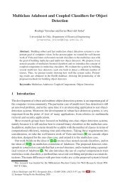
J Intell Robot Syst (2012) 66:125–149 137dating is not available, a C version of the zchddsubroutine from LINPACK library [27], originallywritten in Fortran, was obtained using fable [28].After each correction step, the quaternioncomponents in state are normalized. To ensurecoherence in the <strong>SLAM</strong>, a Jacobian from thenormalizing function is used to propagate normalizationeffects into the state covariance matrix.5. Inverse-depth landmarks collapsing. Inversedepthlandmarks whose uncertainty drops belowa threshold are converted into normalpoint-like landmarks.6. Point-like landmarks collapsing. The covarianceof points P pp is analyzed in order toverify if a set of point-like landmarks existsthat can generate a rigid-body landmark. Asexplained in Section 3.3, the procedure requiresverifying whether a variability indexassociated with a set of point-like landmarksis below a threshold th (Eqs. 29, 30, 31). Incase a rigid-body landmark can be generated,the procedure described in Section 3.2 is used(Eqs. 9, 10, 11, 12, 13, 14, 15, 16, 17, 18, 19, 20,21, 22, 23, 24, 25, 26).7. Inverse-depth landmarks generation. ImageSURF features that were not matched, i.e.they are distant from landmarks in the imagedomain, are added as new inverse-depthlandmarks, using the procedure described inSection 4.1. By selecting an appropriate distancethreshold, the density of observed descriptorsin the image can be kept within adesired range.8. Inverse-depth landmarks deletion. Newinverse-depth landmarks need to be observedfor a certain number of frames in order to beconfirmed. If the number of frames in whichan inverse-depth landmark was not observed,but was expected to be, is over a certainthreshold, the landmark is deleted.5 Experimental Evaluation5.1 Simulated ExperimentsThe system is evaluated by simulating the movementof a camera using four types of trajectories,and applying different visual <strong>SLAM</strong> approachesfor recovering the camera’s path. In all cases thesimulated camera moves looking all the time ata fixed point. The following six trajectories areused, which have closed form for repeatabilitypurposes.1. U-shaped path– Trajectory: x =−60 sin ( π2 sin ( 2π 8)) t , y =−90 cos ( π2 sin ( 2π 8)) t , z = 0– Camera looking at position (0,0,0)2. S-shaped path– Trajectory: x =−40 1+t54 cos ( cos ( ))t3t , y =40 1+t54 sin ( cos ( ))t3t , z = 0– Camera looking at position (30,0,0)3. Continual Lost path– Trajectory: S-shaped path (80 s) followedby a square path with four very distantpoints (−90, −40), (−90, 40), (−30, 40),(−30, −40). Each periodic sequence takes4 s, and the transition between the fourpoints is done without any delay.– Camera looking at position (30,0,0)4. S-shaped+Random-Walk path– Trajectory: S-shaped path (80 s) followedby a random walk: x t = x t+1 + n X , y t =y t+1 + n Y , z t = z t+1 + n z , n X , n Y , n Z →N (0, 100) .– Camera looking at position (30,0,0)The trajectories were sampled into controlpoints by using a 1 s step. Intermediate pointswere calculated by using spline interpolation inthe point-quaternion space. A set of 900 SURFdescriptors are generated randomly in a 400 × 400square area centered at the origin of the globalcoordinate system by using a uniform distribution;64D values for the SURF descriptors areinitialized in a random way by using a uniformdistribution followed by a normalization. Some ofthe descriptors will give rise to landmarks whenobserved by first time, and then each landmarkcorresponds to a unique known feature in space,which enables comparing landmarks and originalfeatures. The frame rate of the simulated camerais 15 fps. Gaussian noise with a standard devia-

138 J Intell Robot Syst (2012) 66:125–149Fig. 1 Simulated cameratrajectories used inexperimentsU-shapedS-shapedContinual LostS-shaped+Random-Walktion of six pixels was added to the observationsin order to simulate noise which is intrinsic toSURF detection process. The simulated camerahas a resolution of 320 × 200. A visualizationexample of each path, showing both the controlpoints and the spline interpolation is shown inFig. 1.Several simulation tests were carried out ineach of the paths. Each test takes 2,800 frames,and it is started with the restriction of having amaximum of 60 landmarks:Test 1:Test 2:Test 3:Test 4:Test 5:Only point-like landmarks are used.All kind of landmarks are used. The maximalpose covariance criterion is used incase of body-point 3D landmarks.All kind of landmarks are used. The maximalbody-points covariance criterion isused in case of body-point 3D landmarks.Only point-like landmarks are used. Themaximum number of landmarks is constrainedto 4 at frame 1,800.All kind of landmarks are used. Themaximal pose covariance criterion is applied.The maximum number of rigidbody landmarks is constrained to 4 atframe 1,800, and no point-like landmarksare used.Test 6:Same as test 5, but the maximal bodypointscovariance criterion is applied.In all cases, point-like landmarks are first createdas inverse-depth landmarks.Given that map building by using a single cameracan produce differences in position, orientationand scale respect to the ground-truth, anoptimal transformation that consider all threecharacteristics is found and applied to experimentalpath for making comparison possible (leastsquares procedure). The average Euclidean distancebetween correspondent pairs of points in theground truth and the computed paths, i.e. pairs ofpoints that correspond to the same time, is used aserror measurement.In Fig. 2 are shown some examples of recoveredpaths together with the corresponding groundtruth. As obtained results need to be analyzedvery carefully, histograms of the errors will bepresented in addition to mean errors and standarddeviation values. In the histograms visualization,errors with values over 60 will be cut to that valorfor maintaining an adequate scale, and they willbe considered failures. Table 1 presents experimentalresults in terms of mean error, standarddeviation, and failure percentage for all experiments,while Figs. 3, 4, 5, 6 shows the histograms

J Intell Robot Syst (2012) 66:125–149 139Fig. 2 Simulationexample of the recoveredpaths drawn over theground truth one for eachkind of path is shown.The set of all features isshown in blue, thesetoffeatures that wereselected as landmarks isshown in green andcurrent landmarks areshown in redU-shapedS-shapedContinual LostS-shaped+Random-WalkTable 1 Experimentalresults of visual <strong>SLAM</strong>for the differenttrajectories and simulatedtestsPath Test Max num. Mean Standard FailureLandmarks error deviation percentageU-shaped 1 60 1.79 0.69 0%U-shaped 2 60 8.02 5.80 0%U-shaped 3 60 3.67 0.84 0%U-shaped 4 4 – – 100%U-shaped 5 4 41.03 16.18 76.7%U-shaped 6 4 4.19 0.93 0%S-shaped 1 60 6.81 3.53 0%S-shaped 2 60 26.12 20.78 86.67%S-shaped 3 60 10.95 6.64 0%S-shaped 4 4 18.34 5.67 90%S-shaped 5 4 – – 100%S-shaped 6 4 13.22 6.52 0%Continual lost 1 60 11.69 3.18 0%Continual lost 2 60 30.07 14.49 70%Continual lost 3 60 25.34 10.9 6.67%Continual lost 4 4 – – 100%Continual lost 5 4 – – 100%Continual lost 6 4 25.75 6.25 0%S-shaped+R 1 60 2.54 1.24 0%S-shaped+R 2 60 20.89 13.66 0%S-shaped+R 3 60 3.80 1.10 0%S-shaped+R 4 4 32.97 7.10 0%S-shaped+R 5 4 29.75 7.87 0%S-shaped+R 6 4 3.57 0.86 0%

140 J Intell Robot Syst (2012) 66:125–14919Test 1 Test 2 Test 330 23Test 4 Test 5 Test 6Fig. 3 Histograms of tests applied over the U-shaped path26Test 1 Test 2 Test 32730Test 4 Test 5 Test 6Fig. 4 Histograms of tests applied over the S-shaped path

J Intell Robot Syst (2012) 66:125–149 14121Test 1 Test 2 Test 330 30Test 4 Test 5 Test 6Fig. 5 Histograms of tests applied over the Continual Lost pathTest 1 Test 2 Test 3Test 4 Test 5 Test 6Fig. 6 Histograms of tests applied over the S-shaped + Random walk path

142 J Intell Robot Syst (2012) 66:125–149Fig. 7 Execution time for<strong>SLAM</strong> prediction-updatesteps versus number offeatures in the mapFig. 8 <strong>Visual</strong>ization example of the <strong>SLAM</strong> system workingin a video sequence. Observations are shown as rhombsover imposed on captured image and innovation covarianceis drawn as a set of ellipses. Point-like landmarks aredrawn as blue dots. Rigid body landmarks are drawn aswhite reference systems with white body points. MatricesC X , C Y and C Z , used to evaluate variability index, areshown bottom left. Full covariance matrix is shown top right

J Intell Robot Syst (2012) 66:125–149 143Fig. 9 Selected images from the garden video database. In each image rhombs correspond to real observations (SURFinterest points), and ellipses represent the innovation covariancefor the errors. In all cases each test was run 30times in every path in order to generate robuststatistics.In the case of the U-shaped, S-shaped, andS-shaped+Random-Walk paths (see Table 1 andFigs. 3, 4, 5, 6), it can be observed that when thenumber of landmarks is limited to 60, the bestoption is to use point-like landmarks, and rigidbodylandmarks using the maximal body-pointscovariance criterion produce a slightly largererror.However, when the number of landmarks isvery small (limited to 4), rigid-body landmarksusing the maximal body-points covariance criterionshow an impressive advantage over pointlikelandmarks, as the reduction of the numberFig. 10 Example of the visual <strong>SLAM</strong> system running inone of the real video sequence. The camera is shown inyellow. Blue dots correspond to point-like landmarks, whilewhite structures consisting in three perpendicular axis anda set of white body points denote rigid-body landmarks

144 J Intell Robot Syst (2012) 66:125–149of landmarks produce only a very weak errorincrease. Even in some cases where the use ofpoint-like landmarks fails completely (U-shapedpath and test 4), the use of rigid-body landmarkswith the maximal body-points covariance criterionbehave appropriately. In all cases the use of theFig. 11 Maps andreconstructed paths forthe seven tested videos.The camera is shown inyellow. Blue dotscorrespond to point-likelandmarks, while whitestructures consisting inthree perpendicular axisand a set of white bodypoints denote rigid-bodylandmarksVideo sequence 1; 1,338 frames.Video sequence 2; 1,134 frames.Video sequence 3; 1,107 frames.Video sequence 4; 1,491 frames.Video sequence 5; 1,469 frames.Video sequence 6; 1,372 frames.Video sequence 7; 1,494 frames.

J Intell Robot Syst (2012) 66:125–149 145maximal body-points covariance criterion appearsas the best option.The Continual Lost path is a very hard test asit involves instantaneous and very large changesof the position of the camera, which can producedivergences in the <strong>SLAM</strong> system. Point-likelandmarks behave better when the number of observedfeatures is high. However, errors involvedin all of the results are very high as they are ofthe same magnitude order than the size of thefull path (around 30). In the case of using justfour landmarks in the map, point-like landmarksare not able to follow the path, failing in all ofthe cases. Rigid-body landmarks with the maximalbody-points covariance criterion are able to followappropriately the path.From the experimental data, it is clear that incases where the number of landmarks needs tobe limited, because of computational reasons orbecause of the large size of the map, the use ofrigid-body landmarks is very useful. In addition,it is evident that it is convenient to propagatethe most possible quantity of covariance fromthe original point landmarks into the body pointcovariances. As the positions of body points arenot adapted before its creation, the error associatedto them does not decrease, and then itscovariances must be constant over time. If thecovariance from the original points is propagatedmainly into the covariance of the pose, covariancefrom rigid-body landmarks will be underestimatedbecause the covariance of the pose decrease tozero when it is observed, and the covariance frombody points remains very low. This fact can causea severe covariance underestimation when observinga landmark several frames before its creation.Then, maximizing propagation of originalcovariance into body point covariances is the bestoption.Execution times for <strong>SLAM</strong>, including both predictionand update steps, were measured as a functionof the number of features used in the <strong>SLAM</strong>system. In the runtime experiment, the path andfeature configuration used in the U-shaped pathtest was selected. As it can be observed in theresults shown in Fig. 7, the ratio between executiontimes for a <strong>SLAM</strong> using only point-likepoints versus a <strong>SLAM</strong> using rigid-body landmarksconverges to the 5.5% limit, as the number offeatures in the map increases. This can be explainedbecause matrix operations in the EKF updatestep become the most expensive computationin <strong>SLAM</strong> when the number of features is high,because of their quadratic nature. Then the stateFig. 12 Camera movingin a polygonal trajectory(f irst), and moving on anelliptical trajectory(second row). In bothcases, the ideal cameratrajectory, as well as themaps and thereconstructed paths areshown3m2m2m1m4m6m

146 J Intell Robot Syst (2012) 66:125–149reduction capabilities of the rigid body approachhave an impressive impact in the execution time.The performance penalty related to the computationof virtual observations is very low whencompared to matrix operations, as they grow in alinear fashion. This experiment was realized in anFig. 13 Recoveredelliptic paths, and errorbetween start and endpointsStart-endpoint error: 2.97%Start-endpoint error: 4.04%Start-endpoint error: 9.80%Start-endpoint error: 4.41%Start-endpoint error: 4.19% Start-endpoint error: 13.67%Start-endpoint error: 6.25%

J Intell Robot Syst (2012) 66:125–149 147Intel Core Duo processor at 1.6 GHz using onlyone core.5.2 Experiments with Real Video SequencesIn a first set of experiments, the system was evaluatedqualitatively. A handheld camera was usedto produce seven video sequences in an outdoorenvironment. In order to generate the sequences,the handheld camera followed a path inside ahouse’s garden. In each of the cases, the pathfinished near its starting point. The camera has anormal lens, the video sequences were captures at30 fps, and their duration in frames is 1,338, 1,134,1,107, 1,491, 1,469, 1,372 and 1494.The proposed visual <strong>SLAM</strong> system using pointlikeand rigid-body 3D landmarks was tested inthese video sequences. The system runs in a standardlow-end laptop. Figure 8 shows a visualizationtool used to analyze the performance of thevisual <strong>SLAM</strong> system in the video sequences. Theposes from rigid bodies are represented by using asmall reference system represented by using threeorthogonal axis x, y, z, which are drawn in white.In Fig. 9 some selected images from the gardenvideo database are shown. Figure 10 shows anexample of the visual <strong>SLAM</strong> system running inone of the real video sequence.In all of the tests the proposed <strong>SLAM</strong> systemwas able to build a coherent map and to recoverthe path. In Fig. 10 the reconstructed paths forthe seven tested videos are shown: the camera isshown in yellow, point-like landmarks are shownas blue dots, and rigid-body landmarks are denoteas white structures.The system was also able to recognize the firstgenerated landmarks (loop closing) easily becauseno tracking is used; instead descriptor matchingbetween the map and the current image’s observationsis done by using L&R system. The robustnessof the matching system is reflected inits capacity to recover the seven paths that weretested (Fig. 11).In a second set of experiments, the systemwas evaluated quantitatively using ground-truthpaths of specific regular shapes. In the initialexperiments, about 40 runs were carried out indifferent environments, using different polygonalpaths containing right angles, but the results wereinaccurate in around half of the cases. The systemwas able to reconstruct the angles from the polygons,but estimations of the sides were not regular,and the estimated pose of camera sometimesmoved long distances when the loop was closed.The explanation found is that straight angles causea loss of the speed information as the camera muststop moving, and features come out of the camerawhen it turns in zones of the path with high curvature.Both problems limit scale preservation. Thisproblem is aggravated by the decision of using astandard narrow-angle camera instead of a wideangle one, which could provide major parallax forthe points when moving. Then, movements of thecamera in visual <strong>SLAM</strong> cannot be arbitrary asthey require some softness, as some parallax onthe features is required to estimate the map, andthe speed of the camera helps to preserve scale.As paths with sharp angles were troublesome,elliptical paths, as the ones shown in Fig. 12,were selected in order to generate seven videosequences for testing purposes. As ellipses havesome degree of rotational symmetry, the mean absoluteerror between the best possible ellipse andthe recovered path can cause an underestimationof the error. This occurs because errors in lengthof the path will not produce errors as long as pathremains into the ellipse. For this reason, the distancebetween the initial and final points from therecovered path was used as a quantitative measureof the accuracy of the proposed system. Figure 13shows the recovered paths and the error betweenthe start and end points, normalized respect tothe length of the ellipse, for ach case. It can beobserved that in most of the cases the start-endpoint error is smaller than 10%, and that its meanvalue is 6.47%.6 ConclusionsIn this work a visual <strong>SLAM</strong> system based on theuse of what are called rigid-body 3D landmarkswas proposed. A rigid-body 3D landmark representsthe 6D pose of a rigid body in space, andits observation gives full-pose information abouta bearing camera. The use of rigid-body 3D landmarkspermits reducing the computational timeof the EKF-<strong>SLAM</strong> system up to 5.5%, as the

148 J Intell Robot Syst (2012) 66:125–149number of landmarks increases. The proposedvisual <strong>SLAM</strong> system was validated in simulateddata and real video sequences using a standard,low cost camera. Remarkably the system performsvery well in outdoor environments, allowing verygood camera localization.The analysis of the visual <strong>SLAM</strong> system operationin real video sequences shows that the implementedsystem has a good performance whentested in the real-world. Rigid-body 3D landmarksare able to reduce the state dimensionality inunstructured environments with low informationloss, which enables the camera to recover the fullpath in a reliable way, avoiding EKF covarianceoverload. SURF descriptors with delayed Harristesting are both fast and repeatable enough toprovide good quality information about structuresin the real-world, even when systems with limitedcomputing capabilities are used. Data associationbased on L&R system, which has been created forrobust object recognition, shows very good performancefor map association tasks and enablesthe EKF to work without map corruption due towrong associations even in long video sequences,and without needing special loop-closing techniquesas all the features have the same opportunityfor being detected in every frame, becauseno features are tracked. Results show that therigid-body landmarks paradigm is both promisingand powerful, and new field application can beexplored in future works.The experimental data indicates that the visual<strong>SLAM</strong> system achieves good localization whenthe number of observed landmarks is very low,working very well with only four landmarks beingavailable for observation permanently, whichis possible by using feature-rich individual landmarks.This property enables them to be used inthe generation of large maps as very few landmarksper area are needed. As body-points areparameters and no states in this system, their errordoes not decrease in time, which can explainthe slight better performance of point-like landmarkswhen the density of landmarks is very high.Possible adaptation of body points by creatinga dynamical sub system inside each rigid bodylandmark (EKF-like adaptation of positions andcovariances from individual body points) and theuse of semantical cues for improving selection ofrigid bodies remains open problems that can beaddressed in future work.Acknowledgments This research work was partiallyfunded by the doctoral grant program of CONICYT(Chile), by MECESUP Project FSM 0601, and by FONDE-CYT project 1090250.AppendixComputation of Jacobians J (i)UVand J(i) , defined in(41)and(42).As function V(·) is the result of an iterativeminimization (see (38)), the computation of J (i)UVand J (i) by using finite differences over severalminimizations is a very slow process. The partialderivatives of E P (·)respect to the pose must bezero when evaluated at the optimal value, thisleads to a closed form for the Jacobians. Forsimplifying the notation, the vector a =(u 1 , v 1 , ..., 1 ,..., N ) T collecting all the parameters will beused in the following expressions:V (a) = arg minη(E P (η; a)) (63)∂∂η iE P (η; a) |η = V (a) = 0, ∀i (64)( )d ∂E P (V (a) ; a) = 0, ∀i, j (65)da j ∂η i∑ ∂ 2 E P ∂V (a) k+ ∂2 E P= 0 ∀i, j (66)k ∂η i ∂η k ∂a j ∂η i ∂a jThe last expression can be converted into matrixform by making the following definitions:E ηη (V (a) ; a) (i. j) = ∂2 E P∂η i ∂η j(67)E ηA (V (a) ; a) (i. j) = ∂2 E P(68)∂η i ∂a jAfter the replacements, the following expressionshold.E ηη (V (a) ; a) ∂V∂a (a) + E ηA (V (a) ; a) = 0 (69)⇒ ∂V (a) =−E−1 ηη∂a (V (a) ; a) E ηA (V (a) ; a) (70)

J Intell Robot Syst (2012) 66:125–149 149The last expression has a closed form, and enablesa straightforward computation of the Jacobiansof V(·). As the quaternion is a non-minimal representationfor rotations, there is a direction inthe observation vector that contains no real information,then variations of the vector in thatdirection leaves the value of the error unmodified.In consequence, the Hessian has a null space andcannot be inverted directly. The problem can besolved by computing the inverse using an eigenvaluedecomposition and by bounding the smallesteigenvalue from the Hessian by a small value (e.g.10 −30 ).References1. Filliat, D., Meyer, J.-A.: Map-based navigation in mobilerobots: I. A review of localization strategies. Cogn.Syst. Res. 4(4), 243–282 (2003)2. Neira, J., Davison, A.J., Leonard, J.J.: Guest editorialspecial issue on visual <strong>SLAM</strong>. IEEE Trans. Robotics24(4), 929–931 (2008)3. Hauke Strasdat, J., Montiel, M. Davison, A.J.: ScaleDrift-Aware Large Scale Monocular <strong>SLAM</strong>, RSS(2010)4. Civera, J, Grasa, O.G., Davison, A.J., Montiel, J.M.M.:1-point RANSAC for EKF-based Structure fromMotion, IROS 2009 Proceedings, pp. 3498–35045. Handa, A., Chli, M., Strasdat, H., Davison, A.J.: ScalableActive Matching, Proc. 2010 IEEE Conf. on ComputerVision and Pattern Recognition, June 13–18,2010, San Francisco6. Davison, A.J., Reid, I.D., Molton, N., Otasse, O.:Mono<strong>SLAM</strong>: Real-time single camera <strong>SLAM</strong>. IEEETrans. Pattern Anal. Mach. Intell. 29(6), 1052–1067(2007)7. Nistér, D., Naroditsky, O., Bergen, J.: <strong>Visual</strong> odometryfor ground vehicle applications. J. Field Robot. 23(1),3–20 (2006)8. Nistér, D.: Preemptive RANSAC for live structure andmotion estimation. Mach. Vis. Appl. 16(5), 321–329(2005)9. Davison, A.J.: Real-time simultaneous localisation andmapping with a single camera, ICCV 2003 Proceedings,pp. 1403–1410 vol. 210. Newcombe, R, Davison, A.J.: Live Dense Reconstructionwith a Single Moving Camera, IEEE Conferenceon Computer Vision and Pattern Recognition (CVPR2010)11. Angeli, A., Davison, A.J.: Live Feature Clustering inVideo Using Appearance and 3D Geometry, BMVC(2010)12. Gee, A.P., Chekhlov, D., Calway, A., Mayol-Cuevas,W.: Discovering higher level structure in visual <strong>SLAM</strong>.IEEE Trans. Robotics 24(5), 980–990 (2008)13. Kwon, J., Lee, K.M.: Monocular <strong>SLAM</strong> with LocallyPlanar Landmarks via Geometric Rao-BlackwellizedParticle Filtering on Lie Groups, 2010 IEEE Conf.on Computer Vision and Pattern Recognition-CVPR2010, pp. 1522–1529, 13–18 June 2010, San Francisco,USA14. Civera, J., Davison, A.J., Martínez-Montiel, M.: Inversedepth parametrization for monocular <strong>SLAM</strong>.IEEE Trans. Robotics 24(5), 932–945 (2008)15. Pathak, K., Birk, A., Vaskevicius, N., Poppinga, J.: Fastregistration based on noisy planes with unknown correspondencesfor 3D mapping. IEEE Trans. Robotics26(3), 424–441 (2010)16. Kohlhepp, P., Pozzo, P., Walther, M., Dillmann, R.:Sequential 3D-<strong>SLAM</strong> for mobile action planning, Proc.2004 IEEE/RSJ International Conf. on IntelligentRobots and Systems, Sendai, Japan17. Pathak, K., Birk, A., Vaskevicius, N., Pfingsthorn, M.,Schwertfeger, S., Poppinga, J.: Online 3D <strong>SLAM</strong> byregistration of large planar surface segments and closedform pose-graph relaxation. J. Field Robot. 27(1), 52–84 (2009)18. Magnusson, M., Lilienthal, A., Duckett, T.: Scan registrationfor autonomous mining vehicles using 3D-NDT.J. Field Robot. 24(10), 803–827 (2007)19. Hamilton, W.R.: On quaternions, or on a new systemof imaginaries in algebra. Philos. Mag. 25(3), 489–495(1844)20. Loncomilla, P.: Generación automática de landmarksvisuales naturales tridimensionales basada en descriptoreslocales para auto-localización de robots móviles,Ph.D. Thesis, Universidad de Chile (2010)21. Bay, H., Ess, A., Tuytelaars, T., Van Gool, L.: SURF:speeded up robust features. Comput. Vis. ImageUnderst. 110(3), 346–359 (2008)22. Haralick, B.M., Lee, Ch.-N., Ottenberg, K., Nölle, M.:Review and analysis of solutions of the three pointperspective pose estimation problem. Int. J. Comput.Vis. 13(3), 331–356 (1994)23. Harris, C., Stephens, M.: A combined corner and edgedetector. Proc. of the 4th Alvey Vision Conference, pp.147–15124. Loncomilla, P., Ruiz del Solar, J.: A fast probabilisticmodel for hypothesis rejection in SIFT-based objectrecognition, Lecture Notes in Computer Science 4225(CIARP 2006). Springer, 696–70525. Ruiz-del-Solar, J., Loncomilla, P.: Robot head posedetection and gaze direction determination using localinvariant features. Adv. Robot. 23(3), 305–328 (2009)26. Welch, G., Bishop, G.: An introduction to the Kalmanfilter. University of North Carolina, Chapel Hill (1995)27. LINPACK library official site: http://www.netlib.org/linpack/28. Grosse-Kunstleve, R.W., Terwilliger, T.C., Adams,P.D.: Experience converting a large Fortran-77 programto C++. IUCr Comp. Comm. 10, 75–84 (2009)