Slope Stabilization Using Recycled Plastic Pins Phase lll

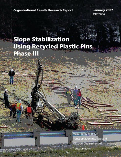
. . . . . . . . . . . . . . . . . . . . . . . . . . . . . . . . . . . . . . . . .Organizational Results Research ReportJanuary 2007OR07.006Slope StabilizationUsing Recycled Plastic PinsPhase lll. . . . . . . . . . . . . . . . . . . . . . . . . . . . . . . . . . . . . . . . .Prepared by MissouriTransportation Institute andMissouri Department ofTransportation

FINAL REPORTRI98-007DSlope Stabilization Using Recycled Plastic Pins – Phase IIIPrepared for theMissouri Department of TransportaionOrganizational ResultsbyJ. Erik Loehr, Ph.D.Assistant Professor of Civil EngineeringandJohn J. Bowders, Ph.D., P.E.Professor of Civil EngineeringDepartment of Civil and Environmental EngineeringUniversity of Missouri - ColumbiaJanuary 2007The opinions, findings, and conclusions expressed in this publication are those of the principalinvestigators and the Organizational Results Division of the Missouri Department ofTransportation. They are not necessarily those of the U.S. Department of Transportation,Federal Highway Administration. This report does not constitute a standard or regulation.

TECHNICAL REPORT DOCUMENTATION PAGE1. Report No. 2. Government Accession No. 3. Recipient's Catalog No.4. Title and Subtitle 5. Report DateSlope Stabilization Using Recycled Plastic Pins – Phase IIIJanuary 20076. Performing Organization Code7. Author(s) 8. Performing Organization Report No.J. Erik Loehr and John J. Bowders9. Performing Organization Name and Address 10. Work Unit No.University of Missouri – ColumbiaDepartment of Civil and Environmental Engineering; E2509 Lafferre Hall11. Contract or Grant No.Columbia, Missouri 65211-2200RI98-007D12. Sponsoring Agency Name and Address 13. Type of Report and Period CoveredFinal Report14. Sponsoring Agency CodeMissouri Department of TransportationResearch, Development and Technology DivisionP. O. Box 270-Jefferson City, MO 6510215. Supplementary NotesThe investigation was conducted in cooperation with the U. S. Department of Transportation, Federal Highway Administration.16. AbstractA new technique for stabilizing surficial slope failures using recycled plastic reinforcing members has been developed. Theobjective of the project described in this report has been to develop, evaluate, and document a technique for stabilization of surficialslope failures using recycled plastic reinforcing members. The project has been undertaken in three sequential phases to provide forlogical evaluation of project accomplishments and refinement of the scope of work based on results of activities undertakenthroughout the project. This report is the final technical report for the entire three phase project, which describes the accumulatedactivities performed throughout all three phases of the project.The principal project tasks undertaken include development of a general design methodology, evaluation of the material properties ofrecycled plastic members from several different manufacturers, establishment of full-scale field test sections at five different sites,monitoring the performance of these sites for periods ranging from two to five years, evaluation and interpretation of fieldobservations, “calibration” of the developed design method, and finally, development of technology transfer materials.The following conclusions are drawn from the work performed as part of this project: (1) the technique of using recycled plasticreinforcement to stabilize surficial slope failures has proven to be effective at providing long-term stabilization; (2) observedperformance at the test sites suggests a typical behavioral pattern consisting of an initial period in which little movement is observedand little load is transferred to the reinforcement, a period of increasing movement and increasing mobilized loads in thereinforcement, followed by a period of stabilized movements and loads in the reinforcing members as a result of the slope coming toequilibrium; (3) while the required member spacing depends on the conditions present at a site, a “standard” pattern that appearssufficient for most sites consists of using recycled plastic reinforcing members placed in a 3-ft by 3-ft (0.9-m by 0.9-m) staggeredarrangement over the entire slide area; (4) reliable installation can be accomplished with either a percussion hammer similar to whatis used on many drill rigs, or a simple drop-weight hammer similar to what is used to install guard rail posts; (5) care must be usedwhen selecting recycled plastic products for use in slope stabilization applications as the properties of these materials can varysubstantially from product to product; and (6) costs for the technique vary with the reinforcement pattern selected but appear to besubstantially less than those for most other competing slope stabilization technologies.Given the cost effectiveness and successful demonstration of the technique, it is recommended that the technique be implemented in“production” operations. The primary challenges to implementation are likely to involve developing appropriate contractingmethods for selection of qualified installation contractors and for acquisition of suitable recycled plastic product. In the early phasesof implementation, it is further recommended that limited monitoring be performed of both construction operations as well as postconstruction performance to further expand the database of cases where the technique has been used and to provide for reliableevaluation of the technique in production operations.17. Key Words 18. Distribution StatementGeotechnical Engineering, slope stability, slope stabilization,recycled plastic, maintenance, repair, field demonstrationNo restrictions. This document is available to the publicthrough National Technical Information Center, Springfield,Virginia 2216119. Security Classification (of this report) 20. Security Classification (of this page) 21. No. of Pages 22. PriceUnclassified Unclassified 289Form DOT F 1700.7 (06/98)

Executive SummaryThe objective of the project entitled "Slope Stabilization Using Recycled Plastic Pins"has been to develop, evaluate, and document a technique for stabilizing surficial slopefailures using recycled plastic reinforcing members. The project has been undertaken inthree sequential phases to provide for logical evaluation of project accomplishments andrefinement of the scope of work based on results of activities undertaken throughout theproject. This report is the final technical report for the entire three phase project, whichdescribes the accumulated activities performed throughout all three phases of the project.Phase I of the project was initiated in January 1999 and served as a “proof ofconcept” phase, wherein a single slope was stabilized using recycled plastic reinforcement.The proof of concept site, located on Interstate 70 near Emma Missouri, was successfullystabilized in November 1999. Additional activities undertaken during Phase I included basiccharacterization of the engineering properties of recycled plastic members, evaluation of thelong-term stability of recycled plastics when subjected to potentially detrimentalenvironmental conditions, and installation of instrumentation for monitoring the performanceof the stabilized slope. Phase I was completed in June 2000.Phase II of the project was initiated in October 2000 to expand the evaluation anddemonstration of the technique. In this phase, test sections were established at five sitesselected from well over 50 candidate test sites to provide for evaluation of the stabilizationtechnique in a variety of different conditions (e.g. slope type, slope height, slope inclination,water conditions, etc.) while at the same time providing opportunity to evaluate alternativestabilization schemes. Two of the selected sites were located in District 4 on Interstate 435in southern Kansas City. Additional sites were located in District 1 on U.S. Highway 36 nearStewartsville Missouri, in District 2 on Interstate 70 near Emma Missouri, and in District 5on U.S. Highway 54 near Fulton Missouri. Following installation, each of the sites weremonitored for periods ranging from two to five years using various types of fieldinstrumentation. Phase II was completed in December 2003.Phase III was initiated in November 2003. The focus of the final phase of the projectwas to complete field monitoring activities at the test sites, to analyze and assimilate theobserved field performance into practical and implementable design and construction toolsand procedures, and to develop practical technology transfer materials to facilitatewidespread implementation of the technique. Field monitoring was completed in February2005. This report serves as the final deliverable for the project and as documentation of theentire three phase project.The principal conclusions derived from the project are as follows:(1) The technique of using recycled plastic reinforcement to stabilize surficial slopefailures in excavated and embankment slopes has proven to be effective atproviding long-term stabilization. To date, slopes stabilized as a part of thisproject have been in place for up to six years. Control sections established atseveral of the sites have failed, which demonstrates that these sites have verylikely been subjected to conditions that are at least as bad as those that caused theoriginal failures and that the installed reinforcement is in fact providing additionalstabilization.i

Loehr and BowdersSlope Stabilization Using Recycled Plastics(2) Observations from field instrumentation measurements taken at the field test sitesprovide a consistent picture of how the reinforcement effects stabilization. Theobserved performance has generally followed a three-stage behavioral pattern. Inthe first stage, the stabilized slopes are observed to experience little movementand little resistance is provided by the reinforcing members. In Stage 2, slopemovements are observed to increase substantially in response to increased porewater pressures within the slope at the same time as loads in the reinforcingmembers are observed to increase. These movements are believed to simply bemovement required to mobilize resistance in the reinforcing members. Finally,Stage 3 is characterized by diminishing movement that is simultaneouslyaccompanied by stabilization of the loads in the reinforcing members. This stageis believed to be a result of the slope and reinforcement coming to equilibrium.(3) The required spacing of reinforcing members depends on the specific conditionsencountered at a particular site. A “standard” reinforcement pattern that appearsto be sufficient for the vast majority of cases encountered consists of a distributedpattern of reinforcing members placed across the entire slide area on a staggeredgrid with members spaced at 3-ft centers. In some cases, appropriate stabilizationcan also be accomplished with members placed at greater spacing.(4) Recycled plastic reinforcing members can be efficiently and reliably installedusing either a percussion hammer found on many drilling rigs or a simple dropweighttype of hammer. Experience acquired to date has shown that the criticalfeature of installation equipment is having a mast to maintain the alignmentbetween the hammer and the reinforcing member.(5) Costs for stabilization of slopes using recycled plastic reinforcing members wererelatively consistent throughout the project. Nominal costs for materials andinstallation are approximately $40/member with the costs being approximatelyequally split between material costs and installation costs. Unit costs per unit areaof the slope face vary significantly with the spacing of the reinforcing members.(6) Field performance data acquired at the respective test sites provide a strong basisfor “calibration” of the general design methodology developed as part of thisproject to establish specific recommendations for application of the method forfuture design. Recommendations developed based on these analyses include:•••that Broms’ (1964) method be used for predicting the limit soil pressure,that axial resistance be ignored in the analyses,that the member capacity used for prediction of member resistance betaken as the nominal measured capacity when members are to be placed atspacings of 3-ft or less and as 60% of the nominal measured capacitywhen members are to be placed at spacings greater than 3-ft.(7) The material properties of recycled plastic members vary with the manufacturingprocess used and the specific blend of constituents used.(8) The properties of all recycled plastic members are dependent on the specificloading rate adopted for testing and the magnitude of loading rate effects can varyfrom product to product. As such, care must be applied when reviewing materialproperties from different manufacturers and for different products to ensure thatacceptable performance can be achieved with a particular product.ii

AcknowledgementsThis project could not have been accomplished without the assistance of numerousindividuals who contributed their time, efforts, and expertise to the project. The assistance ofall of these individuals is gratefully appreciated. Particular acknowledgement is due toThomas Fennessey, Bill Billings, Bruce Harvel, Ken Markwell, Barry Arthur, MikeMcGrath, Steve Giffen, Gary Goessmann, Chuck Sullivan and many others with the MissouriDepartment of Transportation for identifying candidate sites and facilitating the project inmany ways. Pat Carr, Terrell Waller, and several others from The Judy Company providedmuch needed expertise, equipment, and assistance with installation at each of the test sites.Professor Hani Salim of the University of Missouri Department of Civil and EnvironmentalEngineering provided sound guidance for evaluating the structural properties of the recycledplastic members. Randy Jolitz of Epoch Composite Products, Rachel Aanenson of BedfordTechnology, and Sabine Zink of Resco Plastics provided recycled plastic members fortesting. The Recycled Materials Resource Center provided supplemental funding to theproject to support development of a draft specification for recycled plastics for use in slopestabilization. The MoDOT Geotechnical Technical Advisory Group is acknowledged fortheir thoughtful review of project reports and pertinent comments and suggestions for theproject. The support of the University of Missouri College of Engineering and Departmentof Civil and Environmental Engineering is also appreciated. Finally, the assistance ofnumerous undergraduate and graduate student research assistants including: Jorge Parra, EngChew Ang, David Hagemeyer, Paul Denkler, Lee Sommers, Awilda Blanco, Daniel Huaco,Joseph Chen, Glen Bellew, Todd Dwyer, Andy Boeckmann, Nick Roth, Deepak Neupane,Graham Jones, Tim Morgan, Abe Smith, Katy Chandler and many others was integral tocompletion of the project.iii

Table of ContentsExecutive Summary................................................................................................................... iAcknowledgements..................................................................................................................iiiTable of Contents..................................................................................................................... ivChapter 1. Introduction ............................................................................................................. 11.1. Motivation.................................................................................................................. 11.2. Background................................................................................................................ 21.3. Structure of Report..................................................................................................... 31.4. Other Project Documentation .................................................................................... 3Chapter 2. General Analysis Methodology and Design Issues................................................. 72.1. General Approach to Stability Analysis .................................................................... 72.2. Stability of Reinforced Slopes ................................................................................... 92.3. Calculation of Limit Lateral Resistance .................................................................. 102.3.1. Calculation of Limit Resistance Based on Soil Failure Modes ...................... 112.3.2. Structural failure modes.................................................................................. 132.4. Calculation of Factor of Safety................................................................................ 172.5. Issues Associated with Estimation of Limit Lateral Resistance .............................. 192.6. Methods for predicting limiting soil pressure.......................................................... 192.6.1. Ito and Matsui ................................................................................................. 192.6.2. Broms’ Method ............................................................................................... 202.6.3. Poulos and Davis Method ............................................................................... 212.6.4. Comparison of Methods.................................................................................. 222.7. Calculation of Limit Resistance for Inclined Reinforcing Members....................... 232.8. Unresolved Issues .................................................................................................... 252.9. Summary.................................................................................................................. 27Chapter 3. Properties of Recycled Plastic Reinforcement...................................................... 283.1. Sources and Manufacturing of Recycled Plastic Lumber........................................ 283.2. Standard Test Methods for Recycled Plastic Lumber.............................................. 303.3. Testing Program....................................................................................................... 323.4. Uniaxial Compression Tests .................................................................................... 343.4.1. Stress-Strain Response.................................................................................... 363.4.2. Uniaxial Compressive Strength ...................................................................... 383.4.3. Modulus of Elasticity...................................................................................... 423.4.4. Strain Rate Effects .......................................................................................... 443.5. Four-Point Flexure Tests.......................................................................................... 483.5.1. Flexural Stress- Center Strain Curves............................................................. 503.5.2. Flexural Strengths ........................................................................................... 503.5.3. Flexural Modulus............................................................................................ 523.6. Flexural Creep Tests ................................................................................................ 533.6.1. Flexural Creep Test Results............................................................................ 563.6.2. Estimation of Creep Life in the Field ............................................................. 603.7. Evaluation of Material Exposure to Potentially Detrimental Environments ........... 613.8. Significant Conclusions from Materials Testing Program....................................... 62iv

Loehr and BowdersSlope Stabilization Using Recycled PlasticsChapter 4. Site Selection......................................................................................................... 644.1. Criteria for Site Selection......................................................................................... 644.2. Site Selection ........................................................................................................... 644.3. Summary.................................................................................................................. 67Chapter 5. Field Instrumentation ............................................................................................ 685.1. Types of Instrumentation ......................................................................................... 685.2. Measurement of Lateral Deformations .................................................................... 685.3. Measurement of Loads in Instrumented Reinforcing Members .............................. 685.3.1. Strain gages..................................................................................................... 695.3.2. Interpretation of strain gage readings ............................................................. 715.3.3. Force-sensing Resistors .................................................................................. 725.3.4. Interpretation of force-sensing resistor readings............................................. 735.4. Measurement of Pore Pressures, Moisture Content, and Soil Suction .................... 755.4.1. Standpipe Piezometers.................................................................................... 765.4.2. Other Moisture Sensors................................................................................... 765.4.3. Utilization of Pore Pressure/Moisture Sensors ............................................... 795.5. Usefulness of Field Instrumentation ........................................................................ 805.6. Summary.................................................................................................................. 81Chapter 6. I70-Emma Site....................................................................................................... 826.1. Site Characteristics................................................................................................... 826.2. Selection of Stabilization Schemes.......................................................................... 866.2.1. Stabilization Schemes for Slide Areas S1 and S2........................................... 866.2.2. Stabilization Scheme for Slide Area S3.......................................................... 876.3. Field Installation ...................................................................................................... 896.4. Instrumentation ........................................................................................................ 896.4.1. Instrumentation Installed During Phase I ....................................................... 896.4.2. Instrumentation Installed During Phase II ...................................................... 906.5. Field Performance.................................................................................................... 916.5.1. Precipitation at the I70-Emma Site................................................................. 926.5.2. Performance of Slide Areas S1, S2, and S3 – November 1999 to December2002................................................................................................................. 936.5.2.a Pore pressure measurements..................................................................... 936.5.2.b Inclinometer measurements ...................................................................... 946.5.2.c Instrumented reinforcing members........................................................... 966.5.3. Performance of Slide Area S3 – January 2003 to January 2005................... 1016.5.3.a Pore pressure measurements................................................................... 1016.5.3.b Inclinometer measurements .................................................................... 1026.5.3.c Mobilized Bending Moments in Reinforcing Members ......................... 1066.5.3.d Failure of control area and failure in Sections B and C.......................... 1066.5.3.e Post-failure investigations....................................................................... 1086.5.4. Performance of Slide Areas S1 and S2 – January 2003 to January 2005..... 1116.5.5. Potential creep in reinforcement ................................................................... 1126.6. Summary................................................................................................................ 114Chapter 7. I435-Kansas City Sites........................................................................................ 1157.1. Site Characteristics................................................................................................. 115v

Loehr and BowdersSlope Stabilization Using Recycled Plastics10.1.2. Installation in Slide Area S3 ......................................................................... 17510.2. Field Installation at I435-Kansas City Sites........................................................... 17910.2.1. Installation at I435-Wornall Road Test Site ................................................. 17910.2.2. Installation at I435-Holmes Road Test Site.................................................. 18310.3. Field Installation at US36-Stewartsville Site......................................................... 18510.4. Field Installation at US54-Fulton Site ................................................................... 18710.5. Comparison of Installation Performance ............................................................... 18910.6. Summary................................................................................................................ 191Chapter 11. Evaluation and Calibration of Design Method.................................................. 19211.1. Method of Calibration............................................................................................ 19211.1.1. Calibration Procedure for Failed Test Sections ............................................ 19211.1.2. Calibration Procedure for Sections Where No Failure Occurred ................. 19311.2. Required Data for Calibration of Limit Resistance ............................................... 19511.3. Establishment of Acceptable Performance Limit .................................................. 19611.4. Calibration for I70-Emma Site............................................................................... 19611.4.1. Site Characteristics Used in Analysis ........................................................... 19611.4.2. Theoretical Field Performance...................................................................... 19811.4.3. Calibration Using Factored Lateral Resistance............................................. 19911.4.4. Calibration Using Combined Axial and Lateral Resistance ......................... 20211.4.5. Calibration Using Reduced Moment Capacity ............................................. 20311.4.6. Calibration Using Baseline Resistance ......................................................... 20511.4.7. Summary of I70-Emma Site Analyses.......................................................... 20511.5. Calibration for US36-Stewartsville Site ................................................................ 20611.5.1. Site Characteristics Used in Analyses........................................................... 20611.5.2. Theoretical Field Performance...................................................................... 20611.5.3. Calibration Using Factored Lateral Resistance............................................. 20911.5.4. Calibration Using Axial and Lateral Resistance........................................... 21011.5.5. Summary of US36-Stewartsville Site Analysis ............................................ 21011.6. US54-Fulton Site Analysis .................................................................................... 21011.6.1. Site Characteristics Used in Analyses........................................................... 21011.7. Calibration for I435-Wornall Road Site ................................................................ 21311.7.1. Site Characteristics Used in Analyses........................................................... 21311.7.2. Theoretical field performance....................................................................... 21711.7.3. Calibration Using Factored Limit Resistance............................................... 21911.7.4. Calibration Using Combined Axial and Lateral Capacity ............................ 21911.8. Summary of Results from Calibration Analyses ................................................... 22011.8.1. Factoring baseline resistance by a constant amount ..................................... 22011.8.2. Factoring limit soil pressure.......................................................................... 22011.8.3. Reduced moment capacity ............................................................................ 22111.8.4. Incorporation of axial load in reinforcing members ..................................... 22111.9. Recommended Methods for Analysis of Slopes with Recycled PlasticReinforcement........................................................................................................ 221Chapter 12. Summary and Conclusions................................................................................ 22312.1. Summary................................................................................................................ 22312.2. Conclusions............................................................................................................ 22412.3. Recommendations for Implementation.................................................................. 225vii

Loehr and BowdersSlope Stabilization Using Recycled PlasticsReferences............................................................................................................................. 227Appendix A. Boring Logs from I70-Emma Site................................................................... 231Appendix B. Boring Logs from I435-Kansas City Sites ...................................................... 245Appendix C. Boring Logs from US36-Stewartsville Site..................................................... 255Appendix D. Boring Logs from US54-Fulton Site............................................................... 264Appendix E. Slope Stability Model Coordinates.................................................................. 277Appendix F. Draft Material Specification ............................................................................ 284Appendix G. Draft Construction Specification..................................................................... 287viii

Chapter 1. IntroductionThe objective of the project entitled "Slope Stabilization Using Recycled Plastic Pins"has been to develop, evaluate, and document a technique for stabilization of surficial slopefailures using recycled plastic reinforcing members. The project has been undertaken inthree sequential phases to provide for logical evaluation of project accomplishments andrefinement of the scope of work based on results of activities undertaken throughout theproject. This report is the final technical report for the entire three phase project, whichdescribes the accumulated activities performed throughout all three phases of the project.1.1. MotivationSlope failures and landslides constitute significant hazards to all types of both publicand private infrastructure. Total direct costs for maintenance and repair of landslidesinvolving major U.S. highways alone (roughly 20 percent of all U.S. highways and roads)were recently estimated to exceed $100 million annually (TRB, 1996). In the same study,indirect costs attributed to loss of revenue, use, or access to facilities as a result of landslideswere conservatively estimated to equal or exceed direct costs. Costs for maintaining slopesfor other highways, roads, levees, and railroads maintained by government and privateagencies such as county and city governments, the U.S. Forest Service, the U.S. Army Corpsof Engineers, the National Parks Service, and the railroad industry significantly increase thetotal costs for landslide repairs.A significant, but largely neglected, toll of landslides is the costs associated withroutine maintenance and repair of “surficial” slope failures. Costs for repair of such slideswere not explicitly included in the above referenced study because of limited record keepingfor these types of slides by most state departments of transportation. However, the authors ofthe TRB study conservatively estimated that costs for repair of minor slides equal or exceedcosts associated with repair of major landslides. This estimate is supported by the MissouriDepartment of Transportation’s (MoDOT) experience with surficial slide problems, whichare estimated to cost on the order of $1 million per year on average. Many other statedepartments of transportation have similar problems with similarly high, or even higherannual costs. All available evidence clearly indicates that the cumulative costs for repair ofmany surficial slides can become extremely large, despite the fact that costs for repair ofindividual slides are generally low. In addition, minor failures often constitute significanthazards to infrastructure users (e.g. from damage to guard rails, shoulders, or portions of roadsurface) and, if not properly maintained, often progress into more serious problems requiringmore extensive and costly repairs.The premise of the project is that slender structural members manufactured fromrecycled plastics can be used to effectively reinforce slopes as illustrated in Figure 1.1. Asshown in the figure, recycled plastic reinforcing members are installed in the slope tointercept potential sliding surfaces and provide the resistance needed to maintain the longtermstability of the slope. Using recycled plastic members for stabilization has severalpotential advantages over more common civil engineering materials. Plastic members areless susceptible to degradation by chemical and biological attack than other structuralmaterials and are lightweight, meaning smaller installation equipment and lower transportcosts. Plastic members also present less of an obstruction if future construction (e.g.1

Loehr and BowdersSlope Stabilization Using Recycled Plasticsunderground utilities) must traverse a stabilized site. Using recycled plastics also hasenvironmental and political benefits as it reduces the volume of waste entering landfills andprovides additional markets for recycled plastic. Development of a cost effective means forusing these materials while providing long-term stabilization therefore clearly has numerousadvantages for agencies like MoDOT.RoadwayFormerSliding SurfacePlastic ReinforcingMembersFigure 1.1Stabilization of surficial slope failures with recycled plasticreinforcement.1.2. BackgroundBecause no previous attempts to utilize recycled plastic members in similarapplications had been undertaken, the project was developed to be performed in three phases.Phase I of the project was initiated in January 1999 and served as a “proof of concept” phase,wherein a single slope was stabilized using recycled plastic reinforcement. The proof ofconcept site, located on Interstate 70 near Emma Missouri, was successfully stabilized inNovember 1999. Additional activities undertaken during Phase I included basiccharacterization of the engineering properties of recycled plastic members, evaluation of thelong-term stability of recycled plastics when subjected to potentially detrimentalenvironmental conditions, and installation of instrumentation for monitoring the performanceof the stabilized slope. Phase I was completed in June 2000.Phase II of the project was initiated in October 2000 to expand the evaluation anddemonstration of the technique and to begin addressing four key issues deemed critical tosuccessful implementation of the technique on a widespread basis. These issues included:• Determining the range of applicability for using recycled plastic members forslope stabilization (e.g. soil type, slope geometry, etc.),• Validating the assumptions inherent in the design methodology and optimizingplacement of reinforcing members,• Establishing the economics of stabilization with slender reinforcement ascompared to other current and potential stabilization measures, and2

Loehr and BowdersSlope Stabilization Using Recycled Plastics• Developing and documenting formal procedures for design and construction ofslope stabilization measures and developing technology transfer materials.The predominant activities undertaken in Phase II included establishing additional test sitesin differing site conditions, initiating additional performance monitoring to determine theload transfer mechanisms for recycled plastic reinforcement, and acquiring additional costdata for the technique. Phase II was completed in December 2003.Phase III was initiated in November 2003. The focus of the final phase of the projectwas, in essence, to address the remaining issues for successful widespread implementation.The primary objectives of Phase III have been to complete field monitoring activities at thefield test sites, to analyze and assimilate the observed field performance into practical andimplementable design and construction tools and procedures, and to develop practicaltechnology transfer materials to facilitate widespread implementation of the technique. Fieldmonitoring was completed in February 2005. This report serves as the final deliverable forthe project and as documentation of the entire three phase project.1.3. Structure of ReportBecause of the critical role played by full-scale field evaluations at the test sites, thisreport is generally organized with respect to the different test sites with several additionalchapters to describe other pertinent activities and findings. In Chapter 2, the generalobjectives and the adopted approach for design of slopes reinforced using recycled plasticreinforcement are presented followed by descriptions of several specific issues associatedwith predicting the resistance provided by reinforcing members. Evaluations undertaken todetermine the engineering properties of recycled plastic members are then described inChapter 3. The general process and criteria used for selection of the respective field test sitesare described in Chapter 4. Chapter 5 describes the instrumentation used to monitorperformance at the respective field test sites.Activities undertaken to establish each of the respective test sites are described inChapters 6 through 9. Each of these chapters contain general descriptions of the site, asummary of soil properties determined for the sites, a summary of the stability analysesperformed, a description of the selected stabilization scheme(s), descriptions of specificinstrumentation, and finally a summary of observations obtained from instrumentation.Chapter 10 then describes the construction methods used and the installation monitoringperformed for each of the respective field test sites.Chapter 11 contains a summary of observations drawn from collective interpretationof observations from the test sites and description of a series of “calibration” analyses used torefine the general design method based on the observed field performance at the field sites.Recommendations regarding design of slope stabilization schemes using recycled plasticreinforcement are also provided in Chapter 11. Finally, Chapter 12 contains a summary ofthe report along with overall conclusions from the project effort.1.4. Other Project DocumentationIn addition to this report, a series of other publications have been prepared duringdifferent stages of the project to document project activities and findings at interim stages ofthe project, to document more narrowly focused tasks performed as part of the project, or tofacilitate implementation of the slope stabilization technique. These publications include3

Loehr and BowdersSlope Stabilization Using Recycled Plasticsproject reports, draft specifications, student theses, and several peer-reviewed publicationspublished in scholarly journals or conference proceedings.Project Reports• Phase I Technical Report – Slope Stabilization Using Recycled Plastic Pins –Constructability (Loehr et al., 2000)• Phase II Technical Report – Slope Stabilization Using Recycled Plastic Pins:Phase II – Assessment in Varied Site Conditions (Loehr and Bowders, 2003)• Material Properties Evaluation Report – Evaluation of Recycled Plastic Productsin Terms of Suitability for Stabilization of Earth Slopes (Bowders et al., 2003)Technology Transfer Documents• Draft AASHTO Material Specification – Standard Specification for RecycledPlastic Pins Used to Stabilize Slopes• Draft MoDOT Construction Specification – Standard Specification forConstruction of Slope Stabilization Measures Using Recycled PlasticReinforcement• Design and Construction Guide – Guide for Design and Construction of SlopeStabilization Measures Using Recycled Plastic Reinforcement (Loehr andBowders, 2006)• One-half day workshop – “Design and Construction Guidance for SlopeStabilization Using Recycled Plastic Reinforcement”, (Loehr and Bowders, 2005)Student Theses• Stability Analysis of Slopes Reinforced with Recycled Plastic Pins, (Liew, 2000)• Reliability-based Analysis of Three Alternative Methods for Repair of SurficialSlope Failure, (Sommers, 2001)• Engineering Properties of Recycled Plastic Pins for Use in Slope Stabilization,(Chen, 2003)• Evaluation of Uncertainties in the Resistance Provided by Slender Reinforcementfor Slope Stabilization, (Parra, 2004)• Calibration of Resistance Provided by Slender Reinforcing Members in EarthSlopes, (Chandler, 2005)• Numerical Investigation of Load Transfer Mechanism in Slopes Reinforced withPiles, (Ang, 2005)Scholarly Articles• “Stabilization of Slopes Using Recycled Plastic Pins," Transportation ResearchRecord: Journal of the Transportation Research Board, (Loehr et al., 2000)4

Loehr and BowdersSlope Stabilization Using Recycled Plastics• "Construction Methods for Slope Stabilization Using Recycled Plastic Pins,"Proceedings of the Mid-Continent Transportation Symposium, (Sommers et al.,2000)• "Stabilization of Infrastructure Slopes Using Recycled Plastic Pins," ExtendedAbstract published in Proceedings of Transportation Systems 2000 Workshop,(Loehr, 2000)• "Slope Stabilization with Recycled Plastic Pins," Geotechnical News, (Bowdersand Loehr, 2000)• “Stabilization of Slopes with Recycled Plastic Pins,” Proceedings of the NSFWorkshop on Geotechnical Composite Systems, (Loehr, 2002)• “Engineering Properties of Recycled Plastic Pins for Use in Slope Stabilization,”Transportation Research Record: Journal of the Transportation Research Board,(Bowders et al., 2003)• “Field Performance of Embankments Stabilized with Recycled PlasticReinforcement,” Transportation Research Record: Journal of the TransportationResearch Board, (Parra et al., 2003)• “Mechanical Stabilization of Earth Slopes Using Recycled Materials,”Proceedings of Beneficial Use of Recycled Materials in TransportationApplications, (Loehr et al., 2003)• “Design Method for Slope Stabilization Using Recycled Plastic Pins,”Proceedings of Geo-Trans 2004: Geotechnical Engineering for TransportationProjects, (Loehr et al., 2004)• “Sources of Uncertainty in Lateral Resistance of Slender Reinforcement Used forSlope Stabilization,” Proceedings of Geo-Support 2004: Drilled Shafts,Micropiling, Deep Mixing, Remedial Methods, and Specialty Foundation Systems,(Parra et al., 2004)• “Slope Stabilization Using Recycled Plastic Pins,” Proceedings of the 55 thHighway Geology Symposium, (Loehr et al., 2004)• “Numerical investigation of limit soil pressure for design of pile stabilizedslopes,” Prediction, Analysis, and Design in Geomechanical Applications, (Anget al., 2005)• “Creep Behavior of Recycled Plastic Lumber in Slope StabilizationApplications,” Journal of Materials in Civil Engineering, (Bowders et al., 2006)The technical reports for Phase I and II (Loehr et al, 2000, and Loehr and Bowders, 2003)serve as formal documentation of progress and results for the project at the completion of therespective phases. The material properties evaluation report (Bowders et al., 2003)documents efforts undertaken to develop knowledge of the behavior of a range of recycledplastic products and to develop a draft material specification for the products when used forthe slope stabilization application. Pertinent content from these reports is included in thepresent report to provide for a complete technical reference on the entire project effort. The5

Loehr and BowdersSlope Stabilization Using Recycled Plasticstechnology transfer documents were generally developed during Phase III of the project.These documents represent the most up-to-date guidance available based on the lessonslearned throughout the entire project. All of the project reports and technology transfermaterials are available from the Missouri Department of Transportation or from projectinvestigators.The student theses and scholarly articles generally describe specific aspects of theproject, often supplemented with related work outside of the project scope, and represent thestate of knowledge at the time of publication. All of the student theses are available from theUniversity of Missouri. The scholarly articles are available from the publishers of therespective articles or through common literature sources.6

Chapter 2. General Analysis Methodology and Design IssuesThe general approach taken for analysis of reinforced slopes, and the one adopted inthis work, is to first establish the resistance provided by individual reinforcing members andthen to incorporate that resistance into classic slope stability analysis procedures to determinethe factor of safety for the reinforced slope. Given the resistance provided by individualreinforcing members, the mechanics of stability analyses incorporating these forces isrelatively well established. Development of the distribution of resistance provided by asingle member is less well established. In this chapter, the general approach taken to analyzethe stability of slopes reinforced with recycled plastic and “strong” reinforcing members isdescribed with particular focus on development of the distribution of resisting force alongreinforcing members. The developed method utilizes a limit state design approach thatconsiders a series of potential failure modes.2.1. General Approach to Stability AnalysisThe general approach adopted for evaluating the stability of reinforced andunreinforced slopes is to first assume a potential sliding surface and then calculate a factor ofsafety for that sliding surface based on consideration of the equilibrium of the free bodyformed by the sliding surface and slope surface as shown in Figure 2.1. For most slopestability analyses, the factor of safety, F, is defined asFree Body∫∫sF = (2.1)τAssumed sliding surfacec , φ,γ ,uστFigure 2.1Free body diagram considered for equilibrium in slope stabilityanalysis.where s is the available shear strength and τ is the mobilized shear stress (stress required tomaintain equilibrium) on the assumed sliding surface. In the general case, the available shearstrength (s) is a function of the normal stress, σ, on the sliding surface and is often expressedusing the Mohr-Coulomb failure criterions = c + σ tanφ(2.2)7

Loehr and BowdersSlope Stabilization Using Recycled Plasticswhere c is the cohesion intercept and φ is the angle of internal friction for the soil on thesliding surface. In terms of effective stresses, the Mohr-Coulomb criterion is expressed ass = c + ( σ − u) tanφ= c + σ tanφ(2.3)where u is the pore pressure on the sliding surface, σ is the effective stress on the slidingsurface, and c and φ are respectively the cohesion intercept and angle of internal frictionexpressed in terms of effective stresses. Substituting Equation 2.3 into Equation 2.1 resultsin the following expression for the factor of safety in terms of effective stresses( c + ( σ − u)tanφ) ( c σ tanφ)∫ ∫ +=∫τ∫F =(2.4)τEquation 2.4 indicates that the factor of safety along an assumed sliding surface is dependenton (1) the Mohr-Coulomb strength parameters ( c and φ ) for the soil on the sliding surface,(2) the normal stress (σ) on the sliding surface, (3) the pore pressure (u) on the slidingsurface and (4) the mobilized shear stress (τ) on the sliding surface. The Mohr-Coulombstrength parameters ( c and φ ) and the pore pressure (u) are assumed to be known. Thedistribution of normal stress (σ) and shear stress (τ) along the potential sliding surface areunknown and must be determined from equilibrium of the sliding body.The most common approach to determine the distribution of normal and shear stressis to use a “method of slices” as depicted in Figure 2.2. In this approach, the sliding body isdivided into a number of vertical slices and equilibrium of the individual slices is consideredto determine the normal and shear forces (or stresses) on the sliding surface and the factor ofsafety for an assumed sliding surface. The process is then repeated for other potential slidingsurfaces until the most critical sliding surface – the surface giving the lowest value of thefactor of safety – is found. The factor of safety associated with the most critical slidingsurface is taken to represent the stability of the slope.Interslice forceWInterslice forceSNFigure 2.2Static equilibrium of individual slice in the Method of Slices.8

Loehr and BowdersSlope Stabilization Using Recycled Plastics2.2. Stability of Reinforced SlopesA similar approach is adopted for reinforced slopes except that a force due to areinforcing member, F R , is added to the other forces on the slices that are intersected byreinforcing members as shown in Figure 2.3. This force is included in development ofequilibrium equations that are used to solve for the overall factor of safety for the slope. It isimportant to point out that the reinforcement force (F R ) may have components bothperpendicular and parallel to the reinforcing member and that F R is considered a knownquantity and must be provided for the stability analysis.Interslice forceWF RInterslice forceSNFigure 2.3Reinforcement force (F R ) on an individual slice in the Methodof Slices.The reinforcement force modifies the factor of safety in several ways. First, thereinforcement force provides a direct resistance to sliding. This direct resistance will alwaystend to increase the factor of safety over that for the unreinforced slope. In addition, thereinforcement force can modify the computed equilibrium normal and shear forces on thesliding surface and thereby change the factor of safety as compared to an unreinforced slope.These forces can either increase or decrease the factor of safety depending on the inclinationof the reinforcement force with respect to the sliding surface and the respective magnitudesof the axial and lateral components of the reinforcement force. Note that for limitequilibrium analyses, forces due to reinforcement are generally taken as the maximumresisting force that can be developed for the reinforcing element. The forces are thereforereferred to as “limit resistances” in this report.In general, the magnitude of the resisting force that is included in the stabilityanalysis varies with position along the reinforcing member. The distribution of thereinforcement force is described by a “limit resistance curve” as shown conceptually in9

Loehr and BowdersSlope Stabilization Using Recycled PlasticsFigure 2.4. The limit resistance curve defines the magnitude of the resisting force providedby the reinforcing member as a function of the location where a potential sliding surfacecrosses the member. As illustrated in Figure 2.5, each reinforcing member on a slope willprovide a resisting force based on the location of the intersection of the sliding surface andthe reinforcing member. The method adopted for computing the limit resistance distributionfor reinforcing members is described in the following section.Figure 2.4Conceptual distribution of limit resistance along a reinforcingmember in a slope.Limit Resistance DistributionsFigure 2.5ReinforcingMembersF RExample of distributions of limit resistance for multiplemembers in a reinforced slope.2.3. Calculation of Limit Lateral ResistanceBecause the resistance provided by reinforcing members is assumed known from theperspective of stability analysis, it is necessary to establish the resistance provided byreinforcing members prior to performing stability analysis. The resistance is generallyestimated using a limit state design approach, and is therefore referred to as the limitresistance. The general method used to estimate the limit resistance is described in thischapter. Specific details recommended for use in estimating the limit resistance for recycledplastic reinforcing members are then discussed further in Chapter 11.10

Loehr and BowdersSlope Stabilization Using Recycled PlasticsIn the method adopted for this work, two general failure mechanisms are consideredto determine the distribution of limit lateral resistance along the reinforcing members: failureof soil around or between reinforcing members and structural failure of the reinforcingmember due to mobilized forces from the surrounding soil. The method only considers thelateral resistance provided by the reinforcing members; axial contributions are ignoredalthough it is clear that axial forces can have an effect on stability. Axial contributions of thereinforcing members are discussed further later in this chapter and in subsequent chapters.Four specific limit states, or failure modes, are considered in determining thedistribution of limit resistance along the reinforcing member as summarized in Table 2.1.The failure mode producing the least limit resistance at each potential sliding depth governsthe magnitude of the overall limit resistance. The following sections describe this process inmore detail.2.3.1. Calculation of Limit Resistance Based on Soil Failure ModesThe limit lateral soil pressure is the maximum lateral pressure that the soil adjacent tothe reinforcing member can sustain before failure, either by flowing around or betweenreinforcing members. The two soil failure modes considered in the method are referred to asFailure Mode 1 and Failure Mode 2. In Failure Mode 1, the soil above the sliding surface isconsidered to fail by flowing between or around the reinforcing members. In Failure Mode2, the soil below the sliding surface adjacent to the reinforcing member is assumed to fail,resulting in the reinforcing member passing through the soil. The limit resistancecorresponding to each of these failure modes is computed based on the limit soil pressure.Table 2.1FailureModeMode 1Mode 2Mode 3Mode 4Summary of soil and member failure modes for establishinglimit lateral resistance of reinforcing members.DescriptionFailure of soil above sliding surface around or between reinforcingmembersFailure of soil below sliding surface due to insufficient anchorage lengthStructural failure of member in bendingStructural failure of member in shearThe limit soil pressure (a stress) and limit lateral resistance (a force) acting on areinforcing member for an assumed sliding depth are illustrated in Figure 2.6. The limitresistance (a force) is computed by integrating the limit soil pressure over the length of thereinforcing member above the depth of sliding, assuming that the limit soil pressure is fullymobilized along the entire length of the member above the sliding surface. The limitresistance force is assumed to act perpendicular to the reinforcing member at the slidingsurface. Since the depth of the critical sliding surface is unknown, the limit resistance iscomputed for varying sliding depths to establish the limit resistance as a function of positionalong the length of the reinforcing member.In Failure Mode 1, the soil above the sliding surface is assumed to fail by flowingbetween or around the reinforcing members. The reinforcing member is assumed sufficientlyanchored into stable soil below the sliding surface. A schematic depicting this idea is shown11

Loehr and BowdersSlope Stabilization Using Recycled Plasticsin Figure 2.7. A limit resistance curve describing the magnitude of the limit lateral resistanceas a function of position along the reinforcing member for Failure Mode 1 is shown in Figure2.8.lsSlidingsurfaceptotalresistance⇒l sSlidingsurfaceP =z=l∫sz=0( )p uzlimit soilpressure,p u( z)(a)z(b)zFigure 2.6Schematic illustrating calculation of limit resistance force: (a)limit soil pressure and (b) equivalent lateral resistance forceSlopeSurfaceReinforcingMemberLimit Resistance (lb/ft)0 100 200 300 400 5000.01.02.0SlidingSurfaceFailedSoilPosition along member (ft)3.04.05.06.0Failure Mode 1RelativeMovement7.08.0Figure 2.7 Schematic illustratingFailure Mode 1.Figure 2.8 Limit resistance curve for FailureMode 1.A similar process is used to calculate the resistance for Failure Mode 2, except thatthe soil below the sliding surface adjacent to the reinforcing member is assumed to fail while12

Loehr and BowdersSlope Stabilization Using Recycled Plasticsthe member is sufficiently anchored in the moving soil above the sliding surface. Thereinforcing member is essentially flowing through the soil below the sliding surface, asillustrated in Figure 2.9. The limit resistance for Failure Mode 2 is determined by integratingthe limit soil pressure along the reinforcing member below the depth of the sliding surface,again assuming that the limit soil pressure is fully mobilized along the length of memberbelow the sliding surface. This calculation is again repeated for varying depths of sliding todevelop a curve describing the magnitude of the limit resistance along the length of thereinforcing member for Failure Mode 2, as shown in Figure 2.10.Limit Resistance (lb/ft)0 100 200 300 400 5000.0Location afterSliding1.02.0SlidingSurfacePosition along member (ft)3.04.05.0FailedSoilRelativeMovementInitialLocation6.07.08.0Failure Mode 2Figure 2.9. Schematic illustratingFailure Mode 2.Figure 2.10 Limit Resistance curve forFailure Mode 2.Combining the two soil failure modes, a composite curve can be developed by takingthe least resistance for the two failure modes to produce the limit resistance along the lengthof the reinforcing member. A typical composite limit resistance curve considering the twosoil failure modes is shown in Figure 2.11. The limit resistance computed in this manner issuitable for cases where the structural capacity of the reinforcing member is such that failureof the soil completely controls the resistance.2.3.2. Structural failure modesUnder some conditions, the limit soil pressure may be great enough that thereinforcing member will fail structurally prior to complete mobilization of the soil resistance.Two potential modes of structural failure exist: failure of the member in bending (FailureMode 3) and failure of the member in shear (Failure Mode 4). Failure Mode 3 can be furtherbroken into two subcategories: failure due to excessive moments from the applied soilpressure above sliding surface (Failure Mode 3a) and failure due to excessive moments fromthe soil pressure below the sliding surface (Failure Mode 3b). Failure mode 3a and the limitresistance curve for Failure Mode 3a are shown in Figures 2.12 and 2.13, while the schematicand limit resistance curve for Failure Mode 3b are shown in Figures 2.14 and 2.15.13

Loehr and BowdersSlope Stabilization Using Recycled PlasticsLimit Resistance (lb/ft)0 100 200 300 400 5000.0Limit Resistance (lb/ft)0 100 200 300 400 5000.01.01.02.02.0Position along member (ft)3.04.05.0Failure Mode 1Position along member(ft)3.04.05.0Composite SoilResistance6.06.07.0Failure Mode 27.0(a)8.0(b)8.0Figure 2.11Determination of composite resistance based on failure of thesoil: (a) Limit resistance curves of Failure Modes 1 and 2 and(b) composite limit resistance curve of Failure Modes 1 and 2.Failure ofmemberin bendingInitial LocationSoilPressureSlidingSurfaceRelativeMovementPosition along member (ft)Limit Resistance (lb/ft)0 100 200 300 400 5000.01.02.03.04.05.06.07.08.0Failure Mode 3aFigure 2.12 Schematic illustrating FailureMode 3aFigure 2.13 Limit Resistance Curve for FailureMode 3a14

Loehr and BowdersSlope Stabilization Using Recycled PlasticsInitial LocationLimit Resistance (lb/ft)0 100 200 300 400 5000.01.0Failure ofmemberin bendingSoilPressureSlidingSurfaceRelativeMovementPosition along member (ft)2.03.04.05.06.07.0Failure Mode 3b8.0Figure 2.14 Schematic illustrating FailureMode 3bFigure 2.15 Limit Resistance curve for FailureMode 3bTo calculate the limit resistance corresponding to structural failure of the member inbending, the maximum moment (M max ) in the reinforcing member is calculated from elastictheory or numerical methods using the computed limit soil pressures. A scaling factor, α, isthen calculated as:M maxM ultα =(2.5)where M ult is the ultimate design moment of the reinforcing member. This scaling factor isthen used to produce a factored soil pressure that approximately produces a maximummoment, M max , equal to M ult . A typical distribution of moment versus depth for a slidingdepth of 3.5-ft. is shown in Figure 2.16. The computed maximum moment using the limitsoil pressure exceeds the capacity of the reinforcing member. The moment is scaled down sothat the maximum moment is equal to the ultimate moment of the reinforcing member, asshown in Figure 2.16a. This scaling factor is then applied to the limit soil pressure, as shownin Figure 2.16b, to produce the factored soil pressure. This factored soil pressure is then usedto compute a limit resistance by integrating the factored pressure over the length of memberabove (mode 3a) or below (mode 3b) the sliding surface as was done for Failure Modes 1 and2. This process is repeated for varying depths of sliding to produce a curve of the limitresistance corresponding to failure of the reinforcing member. A typical plot of this limitresistance for Failure Modes 3a and 3b is shown in Figure 2.17.The limit resistance due to failure of a reinforcing member in shear can be evaluatedin a similar manner to failure of the reinforcing member in bending by determined thefactored soil pressure that causes the computed maximum shear to equal the shear capacity of15

Loehr and BowdersSlope Stabilization Using Recycled Plasticsthe reinforcing member. For the members considered in this research, the shear capacity isnot a controlling limit state at any point along the length of the reinforcing member.Moment (lb-ft)-500 0 500 1000 1500 2000 2500 3000 350001Moment Capacity, M ult23M ultDepth (ft)4567Factored MomentDistribution, α M maxα =0.32Unfactored MomentDistribution, M max(a)8Soil Pressure (lb/ft)00 100 200 300 400 500 600123Unfactored limit soilpressureDepth (ft)456(b)78Figure 2.16Factored soil pressureα = 0.32Illustration of method for computing resistance based onbending failure of members: (a) factored moment distributionand (b) factored limit soil pressureCombining the limit resistance curves due to soil failure and the failure of themember in bending, a composite limit resistance curve that accounts for all failure modes can16

Loehr and BowdersSlope Stabilization Using Recycled Plasticsbe established, as shown in Figure 2.18. The controlling failure mode is dependent on thedepth of sliding. For sliding surfaces passing through the upper 2- to 3-ft. of the reinforcingmember, Failure Mode 1 typically controls. Failure Mode 3 controls for sliding surfacespassing through depths of 3- to 7.5-ft. along the reinforcing member. Below that depth,Failure Mode 2 typically controls. These depths are approximate and vary with theproperties of the reinforcing members, the spacing of the members, and the soil properties.Limit Resistance (lb/ft)0 100 200 300 400 5000.0Limit Resistance (lb/ft)0 100 200 300 400 5000.01.02.0Failure Mode 3a1.02.0Composite MemberResistancePosition along member (ft)3.04.05.0Position along member (ft)3.04.05.06.06.07.0Failure Mode 3b7.08.08.0Figure 2.17(a)(b)Limit resistance for structural failure of member in bending: (a)limit resistance of Failure Modes 3a and 3b and (b) compositemember resistanceFor “strong” reinforcing members, the limit soil resistance is not great enough toresult in structural failure of the member. In such cases, the composite limit resistance curveis solely a function of the limiting soil resistance as shown in Figure 2.11b. The limitresistance curve for a “weak” reinforcing member, e.g. Figure 2.18b, is dependent on all fourlimit states. The increased resistance of “strong” reinforcing members as compared to that of“weak” members only produces additional stability if the depth of the critical sliding surfacepasses in the range where the structural capacity of the weak reinforcing member wouldcontrol (Parra, 2004).2.4. Calculation of Factor of SafetyOnce the overall limit lateral resistance distribution is developed for individualreinforcing members, the mechanics of stability analysis for slopes reinforced with structuralmembers are relatively straightforward and well established. The commercial slope stabilityanalysis programs, UTEXAS4 and Slide 5.0, were used to perform all of the stabilityanalyses presented in this report. Both programs have the ability to search for the most17

Loehr and BowdersSlope Stabilization Using Recycled Plasticscritical sliding surface and the minimum factor of safety with or without reinforcingelements.Position along member (ft)Limit Resistance (lb/ft)0 100 200 300 400 5000.0Failure Mode 11.0Failure Mode 3a2.03.0Failure Mode 3b4.05.06.0Position along member (ft)0 100 200 300 400 5000.01.02.03.04.05.06.0MemberFailureLimit Resistance (lb/ft)Composite LimitResistanceSoil Failure7.08.0Failure Mode 27.08.0Soil FailureFigure 2.18(a)Determination of composite limit resistance curve for allfailure modes: (a) limit resistance curves for Failure Modes 1,2, and 3 and (b) Composite limit resistance curve(b)Although the process of calculating the factor of safety using UTEXAS4, Slide, orother suitable software is straightforward once the overall limiting lateral resistance curve isdeveloped, the searches for the most critical sliding surface (the surface giving the minimumfactor of safety for a particular set of slope conditions) proved to be difficult as numerous“local minima” exist as sliding surfaces passing through different zones of the reinforcementare considered. To ensure that the overall most critical sliding surface was found for allanalyses, a rigorous search procedure was developed. The procedure consisted of:1. selecting several starting centers of circles for the searches (6-10) around thetoe, face and crest of slope;2. for each center of circle chosen, trying a radius crossing reinforcement withthe sliding surfaces less than 4 ft (1.2-m) and 8 ft (2.4-m) below the face ofthe slope;3. from the most critical circle found from step (2), repeat searches by startingthe search using circles with the same center and varying the radius withinapproximately 2-ft (0.6-m) of the radius of that previous critical circle. Thecritical circle was determined to a precision of 0.5 ft (0.15-m). This procedureproved to be effective for finding the minimum factor of safety within atolerance of 0.001.18

Loehr and BowdersSlope Stabilization Using Recycled Plastics2.5. Issues Associated with Estimation of Limit Lateral ResistanceWhile the procedure described in Section 2.3 for estimating the limit lateral resistancefor reinforcing members is sound, the mechanics of load transfer in reinforcing members arecomplex and require careful consideration of several potentially important issues. Foremostamong these are:1. the properties of the recycled plastic reinforcing members;2. the magnitude of the limit soil pressure and how it is affected by memberspacing; and3. the effect of member inclination, particularly in regards to the relativemagnitudes of axial and lateral resistance.Further discussion of the properties of recycled plastic members is provided in Chapter 3.The following sections provide additional discussions about the magnitude of the limit soilpressure and the effects of member spacing and inclination. Subsequent chapters thenprovide further discussion of these issues based on observations made at field test sitesduring this project.2.6. Methods for predicting limiting soil pressureAs described in previous sections, the limit soil pressure is a key parameter forpredicting the resistance provided by reinforcing members. Unfortunately, the limit soilpressure resulting from mass movement of soil adjacent to reinforcing members is difficult topredict. A variety of methods exist to estimate the limit soil pressure. However, the limitsoil pressures predicted by these methods vary by a significant amount. Three of the mostcommonly cited methods, by Ito and Matsui (1975), Broms (1964), and Poulos and Davis(1980), are described here.2.6.1. Ito and MatsuiIto and Matsui (1975) proposed a method to determine the limit lateral force onstabilizing piles in a slope. The method was established based on soil failure between pilesassuming the soil between the piles to be in a plastic state according to the Mohr-Coulombfailure criterion. This method is referred to as the “theory of plastic deformation”.The assumed region of plastic behavior is shown in Figure 2.20. The followingassumptions are also made:4. Under deformation, two sliding surfaces occur along lines AEB and A’E’B’.5. The soil is plastic only in region AEBB’E’A’6. No frictional forces act on the surface of the pile.7. The soil is assumed to be in a plane strain condition in the vertical direction.8. The piles are rigid.9. The ground surrounding the piles is horizontal.The lateral force provided per unit length of pile is taken to be the difference in soil pressuresacting on surfaces BB’ and AA’ when the soil is in a plastic state.19

Loehr and BowdersSlope Stabilization Using Recycled Plasticsbassumed zone ofplastic behaviorDBFReinforcingMembersD 2AA'CEE'D 1Direction ofdeformationB'F'Figure 2.20Schematic showing assumed region of plastic deformation fortheory by Ito and Matsui (after Ito and Matsui, 1975).The resulting force per unit length of pile at a given depth, z, is obtained by the followingequation:where⎛ ⎞⎝D1P(z)= cD⎜⎟1⎝ D2⎠⎜⎛ 1 tanφ+ NN 2 φ −1⎟⎞φ⎠1 −⎧2⎪ 2tanφ+ 2Nφ+ Nφ−c⎨D112⎪⎩Nφtanφ+ Nφ−1⎡⎢⎢N⎣12φ1tan⎪⎧⎛ D⎞1− D2⎛πφ ⎞⎨exp⎜ N × ⎜ + ⎟⎟φtanφtan − 2Nφ ⎪⎩ ⎝ D2⎝ 8 4⎠⎠−122 φ−2D NN = tan 2⎜⎛ π + ⎟⎞⎝ 4φφ,2 ⎠⎫ ⎧ ⎜⎛⎪ ⎛ ⎞⎝⎪ γzD1⎬+⎨D⎜⎟1Nφ⎪⎭ ⎪ ⎝ D2⎠⎩Nφ12tanφ+N −1⎟⎞φ⎠φ12⎪⎫2tanφ+ 2Nφ+ Nφtanφ−1⎬+12 ⎪⎭ N tanφ+ N −1⎫⎛ D⎞1− D2⎛πφ ⎞ ⎪× exp⎜ N ⎜ + ⎟⎟φtanφtan − D2⎬⎝ D2⎝ 8 4⎠⎠⎪⎭φ12φ−12⎤⎥⎥⎦(2.6)D 1 is the center to center pile spacing, D 2 is the inner distance between piles, c is the cohesionintercept of the soil, γ is the unit weight of the soil, and φ is the angle of internal friction ofthe soil.The limit lateral force on the pile, P, increases linearly with increasing γ or z. For aconstant pile diameter, the limit lateral force also increases as the distance between pilesdecreases. Thus, more closely spaced piles will produce higher limit loads and converselymore widely spaced piles produce lesser limit loads. The limit lateral force also increases asc or φ increases. This is attributed to soils with higher strengths being harder to pass betweenthe piles.2.6.2. Broms’ MethodBroms (1964) presents a method for determining the limit lateral resistance forcohesionless soil surrounding a pile. Different pile lengths and different pile head conditionswere evaluated. The ultimate lateral pressure was assumed to equal three times the Rankinepassive pressure of the soil. Broms assumed that passive lateral earth pressures develop atthe front of the pile (upstream side) and active pressures develop at the back (downstream20

Loehr and BowdersSlope Stabilization Using Recycled Plasticsside). The active lateral earth pressures are small compared to the passive lateral pressuresand are neglected. The lateral earth pressure developed at failure is assumed to beindependent of the cross sectional area of the pile. The limit lateral force per unit depthincreases linearly from zero at the ground surface, with the distribution, P, given by thefollowing equation:P ( z)= 3Dσ'vK p(2.7)where D is the pile diameter, σ v ’ is the effective vertical stress at the depth of interest, and K pis the coefficient of passive earth pressure calculated by the following equation:1+sinφKp=(2.8)1−sinφwhere φ is the angle of internal friction of the soil. Broms’ method assumes lateraldeflections are large enough to develop full passive pressure adjacent to the pile.2.6.3. Poulos and Davis MethodPoulos and Davis (1980) estimated the limit lateral resistance for purely cohesive (φ =0) soils and c-φ soils. For purely cohesive soils, the ultimate lateral soil resistance isassumed to increase from the surface down to a depth of three pile diameters and to remainconstant at depths below three pile diameters. When the ultimate lateral resistance becomesconstant, failure consists of plastic flow of soil around the pile. At the surface, the limitresistance is approximately 2c u , where c u is the undrained shear strength of the soil. Thelimit resistance then increases to a constant resistance of 8 to 12c u at depths of three or morepile diameters below the surface, as shown in Figure 2.21.Lateral Load PPile2cuZd3D8 to 12cuFigure 2.21Distribution of lateral soil resistance for purely cohesive soilsaccording to Poulos and Davis (after Poulos and Davis, 1980).21

Loehr and BowdersSlope Stabilization Using Recycled PlasticsFor purely cohesive soils, the limit soil pressure, p u , is determined by the followingequation:p = K c(2.9)uwhere K c is a lateral resistance factor and c u is the undrained shear strength of the soil. K cdepends on the ratio of pile adhesion to soil cohesion (c a /c) and on the aspect ratio of the pilecross section (d/b) where d and b are the length and width of the pile cross section. Thevariation of the lateral resistance factor, K c , for rough (c a /c=1.0) and smooth (c a /c=0) piles isshown in Figure 2.22.cuFigure 2.22Lateral resistance factors for rough and smooth piles in purelycohesive soils (from Poulos and Davis, 1980).For soils having both a cohesion intercept and an angle of internal friction, theultimate resistance at any depth can be determined by the following expression:p = qK + cK(2.10)uwhere q is the vertical overburden pressure and c is the cohesion intercept of the soil. K c andK q are lateral resistance factors taken to be a function of the friction angle of the soil and theratio of the depth of interest to the width of the pile (z/d). K c and K q are plotted in Figure2.23.2.6.4. Comparison of MethodsParra (2004) compared methods for predicting the limit soil pressure for slenderreinforcing members. A typical plot showing the variation of limit soil pressure amongmethods is shown in Figure 2.24. The variability in the predicted limit soil pressures by thethree methods presented is approximately an order of magnitude. One of the objectives ofthe work described in this report is to evaluate the appropriateness of these methods forpredicting the limit soil pressure based on performance of several field test sites reinforcedwith slender reinforcing members.qc22

Loehr and BowdersSlope Stabilization Using Recycled PlasticsFigure 2.23Lateral resistance factors for c-φ soils (from Poulos and Davis,1980).Depth (ft)0123456789Limit Soil Pressure (psf)0 200 400 600 800 1000 1200 1400φ' = 25 oc' = 0γ = 125 pcfS l = 3-ftIto and Matsui Broms PoulosFigure 2.24Variation in limit soil pressure predicted by different methods(from Parra, 2004)2.7. Calculation of Limit Resistance for Inclined Reinforcing MembersThe limit soil pressure utilized in computing the limiting resistance distributions asdescribed in Section 2.3 is based on the assumption of vertical reinforcing members inhorizontal ground as shown in Figure 2.25. How the limit soil pressure changes for verticalreinforcing members in a slope (Figure 2.26) or for inclined reinforcing members (Figure23

Loehr and BowdersSlope Stabilization Using Recycled Plastics2.27) is not well understood. No other methods appropriate for these conditions were foundin the literature. As such, several approximations were made for using the limit soilpressures for vertical members in sloping ground and for inclined members. Analyses werethen performed to study the impact of the modification in calculating limiting soil pressure.Horizontal GroundReinforcingmemberzFigure 2.25Reinforcing member and ground geometry generally assumedin calculation of limit soil pressure (vertical member inhorizontal ground).For vertically oriented reinforcing members in sloping ground, the limit soil pressurewas assumed to be identical to that computed for vertical members in horizontal ground.While the influence of this approximation is not known at this time, it is believed to havenegligible effect on the limiting resistance of reinforcing members since the effectiveoverburden stress (γz) acting on a reinforcing member at a depth z is similar to that whichwould be computed for horizontal ground (Figure 2.26).Sloping GroundβReinforcingmemberzFigure 2.26Vertical reinforcing member in sloping ground.For inclined reinforcing members, the picture is much less clear. As shown in Figure2.27, the effective overburden pressure at a point at distance z from the top of the reinforcingmember is not given by γz, but rather is a function of the relative inclination of the slope and24

Loehr and BowdersSlope Stabilization Using Recycled Plasticsthe reinforcing member. Two alternative methods for calculating the limit soil pressure weretherefore evaluated for use with inclined reinforcing members. The first alternative used wasto simply ignore the influence of inclination and use the limiting resistance distribution forthe reinforcing members as if they were placed vertically. The second alternative used wasto compute the limiting soil pressure assuming that the effective overburden stress is givenby the height of soil above a particular point on the reinforcing member as shown in Figure2.27. For reinforcing members placed perpendicular to the face of the slope, the verticaloverburden pressure for the second alternative is given byγσ = zvcos β(2.11)where γ is the unit weight of the soil, z is the distance from the ground surface to the point ofinterest measured along the reinforcing member, and β is the inclination of the slope.βSloping Groundzcos βzReinforcingmemberFigure 2.27Inclined reinforcing member in sloping ground.Figures 2.28 and 2.29 show limit resistance curves for “weak” and “strong”reinforcing members respectively placed perpendicular to the face of the slope using the twoalternative methods for computing the limit soil pressure. As shown in the figures, thedifferences in the computed limit resistance curves are small and therefore are not likely tosignificantly influence the computed factors of safety. Additional calculations comparingfactors of safety computed using the two alternative methods described above suggest asimilar conclusion (Liew, 2000).2.8. Unresolved IssuesThe general approach described in this chapter provides the basis for evaluating thestability of slopes reinforced with recycled plastic members. However, several specificissues associated with the analysis procedure remain unresolved. The two most significantissues are:1. Which method for predicting the limit soil pressure is most appropriate, and2. What is the influence of member inclination, particularly as related to relativeaxial and lateral resistance components?25

Loehr and BowdersSlope Stabilization Using Recycled Plastics012Limit Resistance Per Unit Length of Slope, F p (lb/ft)0 20 40 60 80 100 120 140 160 180 200without Without cos cos β betawith With cos cos β (beta)Sliding depth, Z s (ft)3456c =0φ =20.4 deg.γ =110 pcfD 1 =3-ftE p I p =19.2 kip-ft 2789Figure 2.28Limit resistance curves for “weak” reinforcing members placedperpendicular to the face of the slope computed using twoalternative methods.012Limit Resistance Per Unit Length of Slope, F p (lb/ft)0 50 100 150 200 250 300 350without Without cos cos β betawith With cos cos β (beta)Sliding depth, Z s (ft)3456c =0φ =20.4 deg.γ =110 pcfD 1 =3-ftE p I p =19.2 kip-ft 2789Figure 2.29Limit resistance curves for “strong” reinforcing membersplaced perpendicular to the face of the slope computed usingtwo alternative methods.Both of these issues are also largely unresolved for other types of reinforcement so littleguidance on these issues is presently available. The limit soil pressure can have a substantialeffect on the computed lateral resistance of members and thus plays a pivotal role incalculating lateral resistance for members, particularly for the range in values predicted by26

Loehr and BowdersSlope Stabilization Using Recycled Plasticsthe different available methods. The effect of member inclination is less well understood.While the results presented by Liew (2000) suggest that member inclination has little effecton the computed limit soil pressure, the more important issue associated with memberinclination is the relative contributions of axial and lateral resistance for different memberinclinations. It is certainly possible that different member inclinations may provide differentlateral resistance mobilization. Even more importantly though is the contribution ofmobilized axial forces and how these components change with inclination. So while it is arelatively simple matter to compute axial capacities of reinforcing members in slopes, it is amuch more difficult matter to determine how axial resistance will be mobilized as comparedto how lateral resistance will be mobilized. This issue has, to date, received little attentionwith most methods simply ignoring either axial or lateral contributions (the one presumed tobe smaller in magnitude) to stability.As a result of these unresolved issues, the “baseline” method utilized throughout theproject, both for parametric analyses and for design of the stabilization schemes utilized atthe test sites, has utilized the Ito and Matsui (1975) method for predicting limit soil pressuresand has ignored potential contributions from mobilized axial resistance. Use of the Ito andMatsui method is believed to introduce some conservatism into the analysis method.Ignoring axial contributions can be conservative or unconservative, depending on theorientation of the member with respect to the direction of soil movement.A final issue that remains with regard to predicting the resistance provided by thereinforcement is estimation of the bending and/or shear capacity of the members over theservice life of the stabilization scheme. Several phenomena could lead to reduction of thecapacity of the members once installed. Of particular note are the potential for creep of theplastic members, the potential for degradation of the members over time, and the potential fordamage to the members during installation. Test results presented in Chapter 3 suggest thatdegradation from exposure and damage from installation are likely to have little effect on thecapacity of the members. There is also evidence that creep will have only a minor influence,at least when the mobilized stresses in the members are low. However, field evidencedescribed in subsequent chapters also suggests that creep may be occurring so this issueremains somewhat unresolved. Fortunately, the performance data acquired in this projectprovides ample data with which to begin addressing these issues.2.9. SummaryIn this chapter, the limit equilibrium method of stability analysis for reinforced andunreinforced slopes was described. While inclusion of the resisting force provided byreinforcement into limit equilibrium stability analyses is conceptually simple, thedetermination of that force is difficult. The general procedure proposed by Loehr andBowders (2003) for computing composite limit resistance curves based on several potentialfailure modes was described in this chapter. The failure modes considered include: (1)failure of soil around or between reinforcing members above the sliding surface, (2) failureof soil around or between reinforcing members below the sliding surface, and (3) structuralfailure of the reinforcing members. Three methods for predicting the limit soil pressure foruse in this procedure were also presented. One of the objectives of this work is to evaluatethese methods based on performance of several field test sites reinforced with recycledplastic reinforcing members.27

Chapter 3. Properties of Recycled Plastic ReinforcementThe engineering properties of reinforcing members are of paramount importance forslope stabilization because of the potential for structural failure of members due to the loadsimposed by moving soil and due to stresses imparted on the members during fieldinstallation. Due to the variety of manufacturing processes and constituent mixes used in themanufacture of recycled plastic products, the engineering properties of commerciallyavailable members can vary substantially.In order to gain a proper perspective of the engineering properties of recycled plasticmembers used for slope stabilization, an extensive testing and analysis program wasundertaken. The program included:1. determining the basic engineering and material properties of commonlyavailable recycled plastic lumber products;2. determining the potential variability of these properties within one productand among various products and manufacturers; and3. determining how these properties change when the material is subjected tovarious potentially detrimental environments.This chapter provides background information regarding common recycled plastic products,describes several pertinent standardized test procedures for measuring properties of recycledplastic products, and describes results obtained from the testing and analysis program.3.1. Sources and Manufacturing of Recycled Plastic LumberThere are many manufacturers of recycled plastic lumber in the United States. Thenumber is currently more than 30, but is variable due to the nature of start-up businesses.Recycled plastic lumber products vary not only due to different manufacturing methods butalso due to the proprietary blends of materials incorporated into the products, which can varyat their source.Recycled plastic lumber products are manufactured from industrial or post-consumerwaste consisting predominantly of polymeric materials (usually high or low densitypolyethylene). Typically, recycled plastic lumber is composed of the following resins(McLaren, 1995):• High Density Polyethylene (HDPE) – 55 percent to 70 percent,• Low Density Polyethylene (LDPE) – 5 percent to 10 percent,• Polystyrene (PS) – 2 percent to 10 percent,• Polypropylene (PP) – 2 percent to 7 percent,• Polyethylene-terephthalate (PET) – 1 percent to 5 percent, and• varying amounts of additives (sawdust, fly ash, and other waste materials) – 0percent to 5 percent.Table 3.1 shows the common resins, their positive characteristics, common uses, andrecycling rate for 2001. In the United States, post-consumer waste has increased at a fasterrate than industrial waste. Post-consumer, plastic bottle recycling increased by 80 millionpounds in 2001 to an all time high of 1,591 million pounds (APC, 2002). The HDPE rawmaterial comes primarily from post-consumer milk jugs while PET comes primarily from28

Loehr and BowdersSlope Stabilization Using Recycled Plasticspost-consumer soft drink bottles. Assuming a 50 percent recycling rate for all waste plastics,the total production of the recycled plastic lumber is estimated to approach 25 billion boardfeet (6254 m 3 ) per year (McLaren, 1995). Therefore, the importance of the recycled plasticlumber industry in recycling of plastics cannot be overemphasized.Table 3.1Resin TypePolyethyleneterephthalate(PET)High DensityPolyethylene(HDPE)Low DensityPolyethylene(LDPE)Polypropylene(PP)Polystyrene(PS)Common recycled plastics used in recycled plastic lumberproducts (Osman et al., 1999)PositiveCharacteristicsCommonOriginal UseHigh strength, Soft drinkexcellent bottles, juicemoisture barrier, containers, foodgood clarity packagingHigh strengthand meltingpoint, goodductilityExcellentclarity,toughness andflexibility, easyto processLow density,high meltingpoint, andexcellentchemicalresistanceLow cost, lowdensity, goodweatheringresistanceMilk containers,oil bottles, filmsand pipesBottles, trashbags, cablesheathing,sheets and filmsCommonRecycled UseBottles, paintbrushes,geotextiles,carpetingPlastic lumber,motor oilcontainers,bottles, drainagepipesFilms, plasticbags, bottlesCarpeting,netting, Flexible packinggeotextiles, containersheavy-duty bagsCups, waterbottles, outdoorfurniture[1] : Data from American Plastic Council survey results (APC, 2002)Egg cartons,video tape casesQuantityRecycled [1] , lbx10 6(Rec. rate [2] , %)834.3(22.1%)750(23.2%)0.2(0.5%)5.7(3.8%)0.1(1.1%)[2]:Percentages shown for PET and HDPE based on virgin resin sales plus recycled resin used inmanufacture of bottles.Manufacturers also use different processes to produce their product (Bruce et al.,1992). The two main processes commonly used are compression molding and extrusionforming. In compression molding, the constituent waste streams are pulverized, blendedtogether, heated until partially melted, and then compression formed in molds. In thisprocess, the raw material is compressed into desired shapes and dimensions and is cured withheat and pressure. Extrusion forming includes similar steps; however, the molten compositematerial is forced through a die of the desired cross-section for the member being produced29

Loehr and BowdersSlope Stabilization Using Recycled Plasticsin lieu of compression into a mold. An advantage of the extrusion process is that it isrelatively easy to manufacture members of any desired length while the compression moldingprocess requires different molds for each different member length. Extrusion forming isgenerally a more efficient process, allowing greater production rates, but is more challengingtechnically. Owing to the endless variety of possible constituents and manufacturingprocesses, the resulting recycled plastic products (often seen in park benches, picnic tables,and decks for homes and marine setting) can have very different engineering properties, evenamong apparently similar materials and sections.Table 3.2 summarizes the composition and engineering properties of plastic lumberproducts from several different manufacturers reported by Breslin et al. (1998).Manufacturers use materials including virgin plastics, post-consumer waste plastics, andvarious plastic mixtures. Breslin et al. (1998) concluded that the engineering properties ofplastic lumber vary depending on the composition of the polymers and additives used inlumber manufacturing. Unit weights ranged from 47 pcf to 60 pcf (7 KN/m 3 to 9.5 KN/m 3 )for different manufacturers. Compressive strength varied from 1700 psi to 3800 psi (11.7MPa to 26.2 MPa). They also found that use of a single polymer (HDPE) and glass fiberadditive resulted in significantly higher modulus of elasticity for plastic lumber (Breslin etal., 1998).Lampo and Nosker (1997) performed compression tests on recycled plastic lumberproducts from multiple manufacturers. Table 3.3 shows a summary of results provided,which clearly demonstrates that products produced by different manufacturers can havesubstantially different material properties. The significant variation in properties shows thatthese materials cannot be considered identical, and they cannot be assumed to performsimilarly in many applications (Lampo and Nosker, 1997).3.2. Standard Test Methods for Recycled Plastic LumberManufacturers of recycled plastic products will generally document a wide variety ofproperties for their products including strength, dimensional stability, water absorption, nailand screw withdrawal, density, and other properties. For slope stabilization applications, thekey properties of interest are strength and stiffness (both axial and bending), and resistance toinstallation stresses as illustrated in Figure 3.1.Installation Durability Bending and Creep Failure Shear FailureFigure 3.1Three potential modes of failure for reinforcing members inslope stabilization applications.30

Loehr and BowdersSlope Stabilization Using Recycled PlasticsTable 3.2ProductEngineering Properties of Plastic Lumber Products (Breslin etal., 1998)CompositionSpecificGravityUnitWeight [1](lb/ft 3 )CompressiveStrength(psi)Young’sModulus(ksi)TensileStrength(psi)TRIMAX HDPE/Glass fibers 0.75 46.80 1740 450 1250Lumber lastEarth carerecycle maidEarth careproductsSuperwoodSelma, AlRutgersUniversityBTW Rec.plasticlumberCommingled recycledplasticPost-consumer milkjugs0.86 53.66 3755 140 14530.79 49.30 3205 93 - 102.5 2550HDPE 0.909 56.72 - - [2] 173.4 - -33% HDPE, 33%LDPE, 33% PP0.82-0.8751.2-54.3 3468 146.2 - -100% Curb tailings 0.944 58.9 3049 89.5 - -60% Milk bottles,15% Detergentbottles, 15% Curbtailings, 10% LDPE0.883 55.1 3921 114.8 - -50% Densified PS 0.806 50.3 4120 164 - -Post-consumer 0.88-1.0154.9-63.0 1840-2801 162 - -[1] : calculated by present authors[2] : data not availableConversion: 1MPa = 145 psi, 1ksi = 6.9 MPaAxial and flexural strength and stiffness are commonly measured by mostmanufacturers and provided in their advertising literature and on company web sites. Theseproperties are generally obtained from tests performed in accordance with three differentASTM standards:• ASTM D6108 – Standard Test Method for Compressive Properties of PlasticLumber and Shapes (ASTM, 2003);• ASTM D6109 – Standard Test Method for Flexural Properties of Unreinforcedand Reinforced Plastic Lumber and Related Products (ASTM, 2005); and• ASTM D6112 – Standard Test Methods for Compressive and Flexural Creep andCreep Rupture of Plastic Lumber and Shapes (ASTM, 1997).Additional information regarding these standards is summarized in Table 3.4. Thesestandards have served to make properties reported by different manufacturers consistent andhave therefore improved comparisons among different products for a particular application.However, the standard test methods were primarily developed for above ground applicationssuch as decks, and are therefore not perfectly suited to the application of slope stabilization31

Loehr and BowdersSlope Stabilization Using Recycled Plasticswhere conditions and loads differ from above ground applications. Of particular importanceis the fact that the ASTM standard test methods require very high loading rates formeasurement of member strength and stiffness. Since the strength and stiffness of plasticsare sensitive to loading rate, and since loading in the slope stabilization application is muchslower than what is used in the standard test methods (on the order of weeks or months ascompared to minutes), it is not reasonable to assume that properties measured using theASTM standards will be appropriate for predicting performance in slope stabilizationapplications. This issue is further complicated by the fact that some products are moresensitive to loading rate than others so it is difficult to convert properties established usingthe standard test methods to properties needed for design of slope stabilization measures.Nevertheless, these standards do provide a baseline for comparison of different products.Some modifications to the ASTM procedures were employed in the testing programdescribed subsequently.Table 3.3Specific Gravity and Results of Compression Tests onRecycled Plastic Lumber (Lampo and Nosker, 1997)UnitWeight [1](lb/ft 3 )Yield Strength(at 2 % strain)(psi)Ult. Strength(at 10 % strain)(psi)Young’sModulus(ksi)SpecificSample Gravity51A 0.28 17.4 709 785 38.01B 0.70 43.8 1381 1885 61.92D (br) 0.86 53.9 1668 2321 85.32D (g) 0.81 50.5 2103 2857 116.01E 0.86 53.8 1769 2422 80.81F 0.79 49.2 2190 2814 108.21j (b) 0.75 47.0 1900 2364 93.31j (w) 0.91 56.7 2161 2828 110.123L 0.79 49.0 1711 1929 191.41M 0.57 35.3 964 1226 57.91S 0.91 56.7 1668 2045 80.51T 0.88 54.9 2248 3118 117.99U 0.77 48.3 1827 2408 86.7Range 0.28-0.91 17.4-56.7 709-2248 785-3118 38-191.4Mean 0.76 47.4 1715 2231 94.5Std. Dev. 0.17 10.8 465 666 37.6[1] : Calculated by present authorsConversion: 1MPa = 145 psi, 1ksi = 6.9 MPa3.3. Testing ProgramFor this project, an extensive series of laboratory tests were performed to evaluate theengineering properties of recycled plastic products from three different manufacturers.Laboratory tests performed included uniaxial compression tests, four-point flexure tests,32

Loehr and BowdersSlope Stabilization Using Recycled Plasticscompressive creep tests, and flexural creep tests. Detailed procedures and results for each setof tests are described in this section.Table 3.4ASTM Standard Test Methods for Plastic LumberASTM Designation Test MethodD6108Standard TestUniaxialMethod forCompressionCompressiveTestProperties of PlasticLumber and ShapesD6109Standard TestMethod forFlexural Propertiesof Unreinforcedand ReinforcedPlastic Lumber andRelated ProductsD6112Standard TestMethods forCompressive andFlexural Creep andCreep-Ruptured ofPlastic Lumber andShapesFour-pointFlexure TestCompressiveCreep andFlexuralCreepPrimary Constraints• Specimen length = 2 x minimum width.• Compressive stress = compressive loaddivided by minimum or effective originalcross-sectional area.• Compressive strength taken at 3% strain ifno clear yield point.• Strain rate = 0.03 ± 0.003 in/in/min(mm/mm/min) and testing time ~ 1 to 5min.• Secant Modulus @ 1% strain.• Support span (length) divided by minimumwidth = 16 (nominally).• Imposed rate of crosshead motion fromequation listed in the standard.• Flexural strength = maximum stress at themoment of rupture.• Secant Modulus of elasticity in flexurefrom equation provided.• Uniaxial loading for compressive creep.• Plot successive creep modulus versus timeat various stresses for linear viscoelasticmaterials.• Four-point loading for flexural creep.• Approximate time schedule forcompressive or flexural creep tests: 1, 6,12, and 30 min; 1, 2, 5, 20, 100, 200, 500,700, and 1000 hours.Tests were performed on specimens from three different manufacturers, denoted asmanufacturers A, B, and C, as summarized in Table 3.5. All members were nominally 3.5 in.x 3.5 in. (90 mm x 90 mm) in cross-section by 8 feet (2.4 m) in length. Details of themember compositions and manufacturing processes were not provided, but members wereseparated into “batches” to ensure consistency within a single batch. One manufacturer(manufacturer A) provided members manufactured in seven different batches, denotedbatches A1 through A6 and A10, over a period of three years. Members in batches A1through A4 were compression-molded products while members from batches A5, A6 andA10 were extruded products. The constituent formula among the first five batches (A1 toA5) was similar with approximately 60 percent low-density polyethylene (LDPE) and 40percent filler material (primarily sawdust). Batches A6 and A10 were produced using a33

Loehr and BowdersSlope Stabilization Using Recycled Plasticshigher percentage of high-density polyethylene (HDPE). Two additional manufacturers(manufacturers B and C) provided specimens of unreinforced members composed of HDPEwith negligible filler and additives. These specimens are denoted as batches B7 and C9.Manufacturer B also provided specimens composed of HDPE reinforced with cut-strandfiberglass reinforcement (batch B8).Table 3.5SpecimenBatchPrincipalConstituentSummary of recycled plastic products tested for this project.Unitweight(lb/ft 3 )Mftg. [1]Process ConditionDepth(in)Width(in)Length [2](in)A 1 LDPE CM Virgin 3.6 3.6 7.0 61.2A 2 LDPE CM Virgin 3.5 3.5 6.9 63.4A 3 LDPE CM Virgin 3.6 3.6 7.1 64.5A 4 LDPE CM Virgin 3.6 3.4 7.0 64.6A 5 LDPE EX Virgin 3.4 3.4 7.1 58.9A 6 HDPE EX Virgin 3.4 3.4 7.0 60.9A10 HDPE EX Virgin 3.5 3.5 7.0 67.6A11 HDPE EX Installed 3.5 3.5 7.0 68.3A12 HDPE EX Installed 3.5 3.5 7.0 68.5A13 HDPE EX Installed 3.5 3.5 7.0 66.8B 7 HDPE EX Virgin 3.4 3.4 6.9 52.9B 8HDPE +Fiber glassEX Virgin 3.4 3.4 6.9 51.9C 9 HDPE EX Virgin 3.5 3.5 7.0 67.9[1]: CM – compression molded, EX - extruded[2]: for uniaxial compression tests.Conversion: 1 in = 2.54 cm, 1 lb/ft 3 = 0.1572 kN/m 3Specimens from batches A1 through A6, A10, B7, B8 and C9 were manufactured atcompany facilities and shipped to the University of Missouri Geotechnical Laboratories fortesting or to the contractor for installation at the field test sites. Each of these batches isconsidered “virgin” material in that they represent materials just following manufacturing. Incontrast, batches A11, A12 and A13 were composed of specimens that had been subjected todriving stresses during installation at field test sites 1 . All specimens in these batches weremanufactured during the same period as batch A10, and thus have a similar constituentformula. Batches A11 and A12 were installed at the I70-Emma site in January 2003 usingtwo distinct methods of installation. Batch A13 was installed at the US54-Fulton site inJanuary 2003.3.4. Uniaxial Compression TestsUniaxial compression tests were performed on specimens cut from full size recycledplastic members. The member cross-section was square with side dimensions of 3.5 inches(90 mm) and a nominal length of 7 inches (180 mm) – twice the minimum width. The testswere conducted using a stress controlled universal compression machine. As shown inFigure 3.2, a steel plate was placed on top of the specimen to make sure the compressive load1 Specimens were taken from exposed portions of members remaining above ground following installation34

Loehr and BowdersSlope Stabilization Using Recycled Plasticswas uniformly distributed across the whole cross-sectional area of the specimen. A dial gagewas placed beneath the steel plate to measure displacement during the test.Figure 3.2Setup for uniaxial compression tests.Axial strain was computed by dividing the incremental displacement of the loadinghead by the initial height of each specimen. A strain rate was determined by dividing theincremental strain by the elapsed testing time. Secant moduli were established at one andfive percent strain as shown in Figure 3.3 from the slope of the straight line connecting zeropercent strain to the corresponding stresses at one percent and five percent strain. Theaverage strain rate was determined by taking the average of all strain rates before the peakstress was reached, as illustrated in Figure 3.4. An average strain rate of approximately0.006 in/in/min (mm/mm/min) was typically used, except for tests performed to evaluatestrain rate effects.35003000Peak StressUniaxial Compression Stress (psi)2500200015001000500E1%E5%0Figure 3.30 2 4 6 8 10 12 14 16 18 20Axial Strain (%)Typical stress-strain curve showing computation of secantmoduli (batch A3).35

Loehr and BowdersSlope Stabilization Using Recycled Plastics0.0140.012Strain Rate (in/in/min)0.0100.0080.0060.004Avg. strain rate0.0020.000Figure 3.40 2 4 6 8 10 12 14 16 18 20Axial Strain (%)Typical plot of axial strain rate versus axial strain showingmethod used to establish strain rates for each test (Batch A3).Two failure criteria were used to establish the compressive strength of the recycledplastic members. The first one was based on using the original cross-sectional area (A o ) ofthe specimen to calculate the compressive stress and using a five percent strain limit as thebaseline to choose the compressive strength. The second criterion was based on using acorrected cross-sectional area (A c ) based on the measured perimeter of the specimen duringtesting to calculate the compressive stress and choosing the peak stress as the compressivestrength. A measuring tape was used to measure the perimeter of the middle section ofspecimens during the compression test (Figure 3.2). The corrected cross-sectional area (A c )was calculated by assuming the measured perimeter was that of a square section, so that3.4.1. Stress-Strain Response⎛ Measured Perimeter ⎞A c= ⎜⎟(3.1)⎝ 4 ⎠Figure 3.5 shows typical uniaxial compressive stress versus axial strain response forboth extruded and compression molded specimens from different manufacturers. As shownin the figure, specimens provided by manufacturer A exhibited a clear peak in the stressstrainresponse, whereas specimens from manufacturers B and C produced no clear peak inthe stress-strain curves when the original cross-sectional area (A o ) is used to compute stress.The observed peak stress for compression molded specimens from manufacturer A occurs atapproximately 5% strain while the peak for extruded specimens occurs at substantially largerstrains. Figure 3.5 also shows that stresses computed using measured cross-sectional areasthroughout testing are substantially lower than those computed using the initial crosssectionalarea.236

Loehr and BowdersSlope Stabilization Using Recycled Plastics4500Uniaxial Compression Stress (psi)4000350030002500200015001000CompressionBatch A4, Using AoBatch A10, Using AoBatch A4, Using AcBatch A10, Using AcExtruded50000 5 10 15 20 25 30Axial Strain (%)(a) typical stress-strain response for specimens from manufacturer A.45004000Uniaxial Compression Stress (psi)35003000250020001500100050000 5 10 15 20 25 30Axial Strain (%)All Extruded ProductsBatch B7, Using AoBatch C9, Using AoBatch B7, Using AcBatch C9, Using Ac(b) typical stress-strain response for specimens from manufacturers B and C.Figure 3.5Typical uniaxial compressive stresses versus axial strainbehavior for recycled plastic specimens.Figure 3.6 shows typical deformed specimens at the completion of uniaxialcompression tests for compression molded specimens from manufacturer A and extrudedproducts from manufacturers B and C. These photographs reveal that compression moldedspecimens from manufacturer A developed clearly defined failure planes, while specimensfrom manufacturers B and C developed no clear failure planes, but exhibited a bulging typeof failure mode. Both observations are consistent with the observed stress-strain response37

Loehr and BowdersSlope Stabilization Using Recycled Plasticswhere compression molded specimens exhibited a clear peak in the stress-strain curves whileextruded products did not exhibit a clear peak. Observed behavior for extruded specimensfrom Manufacturer A was generally more similar to that shown in Figure 3.6b for otherextruded specimens.(a) Typical failure mode for compression molded specimens from manufacturer A.(b) Typical failure mode for extruded products from manufacturers B and C.Figure 3.6Failure modes for recycled plastic specimens during uniaxialcompression tests.3.4.2. Uniaxial Compressive StrengthObservations from the laboratory testing suggest that a corrected cross-sectional areashould be used in the determination of the compressive strengths, but no standard areacorrection has been established. If one assumes a constant specimen volume and that thecross-section remains uniform during compression, a corrected cross-sectional area can becomputed as:A 0A = e ( 1− ε )(3.2)where A e is the corrected cross-section area, A o is the original cross-sectional area, and ε isaxial strain. However, observation of specimens during testing indicate that the cross-38

Loehr and BowdersSlope Stabilization Using Recycled Plasticssectional areas do not remain uniform and the volume is likely not constant duringdeformation, thus invalidating the use of Equation 3.2 for area corrections. Since noconsistent area correction has been agreed upon, the compressive strengths reportedsubsequently were taken to be the compressive stress at five percent axial strain for allspecimens without area corrections. In cases where a peak stress was exhibited at strains ofless than five percent, the compressive strengths were taken to be equal to the peak stress.The five percent strain limit serves to limit the magnitude of errors associated with thespecimen area and provides a consistent basis for comparison of strengths for differentspecimens. The five percent strain limit also serves as a basis for limiting deformation in thefield applications.Figure 3.7 shows the difference between the “measured” cross sectional area (A c )determined from the measured perimeter during the testing and the original area (A o ) versusaxial strain for specimens from several batches. In general, the cross-sectional area is afunction of axial strain with the area increasing with axial strain for all specimens from allthree manufacturers. The cross sectional area for batches A4 (compression molded) rapidlyincreases while the cross sectional area for batches B7, B8, and C9 increased at a lower rate.The cross sectional areas for batches A5, A6, and A10 (all extruded products frommanufacturer A) have intermediate increases. Application of this correction produces a moreclearly defined peak in the stress-strain response for specimens from manufacturers A, B, andC (Figure 3.5).Difference Between Corrected Area and Initial Area(A c -A o ) (in 2 )Figure 3.74.03.53.02.52.01.51.00.50.0Compression0 5 10 15 20 25 30Axial Strain (%)ExtrudedA o = 11.6 in 2 except forA10, where A o = 12.2 in 2A4A6B7C9A5A10B8Difference calculated from measured perimeter versus axialstrain during compression tests (Mftg A, B, and C).Table 3.6 shows a summary of uniaxial compressive strengths determined from eachbatch. Overall, measured average compressive strengths range from 1600 psi to 3000 psi (11MPa to 21 MPa) when established using the original cross-sectional area. The results shownare for specimens loaded using a nominal strain rate equal to 0.006 in/in/min (0.006mm/mm/min).39

Loehr and BowdersSlope Stabilization Using Recycled PlasticsSpecimens from batches A1 to A4 are compression-molded products with dates ofmanufacture spanning two years. The average strength of these specimens is 2800 psi (19MPa) with a standard deviation of about 150 psi (1 MPa). This shows a good consistency ofproduct over the two-year period. Specimens from batches A5 and A6 were manufacturedusing the extrusion process with a slightly lower amount of “filler” material (primarilysawdust). The average compressive strength of these specimens was 1600 psi (11 MPa),approximately 40 percent lower than specimens from batches A1 to A4. Most of thereduction in strength among specimens in batches A1-A4 and batches A5-A6 is attributed tothe manufacturing process. However, specimens in batches A5 and A6 represent the initialattempts by manufacturer A at extruded products. Specimens from batches A10 to A13 werealso manufactured using the extrusion process. The average strength of these specimens is2200 psi (15 MPa), approximately 20 percent lower than specimens from batches A1 to A4.The subsequent products (Batches A10 to A13) show about a 30 percent increase in theaverage compressive strength of batches A5 and A6. This demonstrates that themanufacturer can modify the process and the constituent mixture to produce materials withcomparable strengths to the compression-molded product.Table 3.6Summary of Uniaxial Compressive Strengths.Nominal Strain Uniaxial Compressive Strength (psi)Specimen # Rate[1]Using A o[2]Using A cBatch Specimens (in/in/min) Avg. Std. Dev. Avg. Std. Dev.A1 10 NA 2784 128 - - [3] - -A2 7 0.005 2948 117 - - - -A3 6 0.005 2824 88 - - - -A4 6 0.005 2621 295 2486 271A5 6 0.007 1634 200 1578 189A6 14 0.007 1602 105 1521 102A10 15 0.006 2219 154 2152 136A11 15 0.006 2301 139 2217 140A12 8 0.007 2085 84 1931 199A13 15 0.007 2380 330 2310 318B 7 15 0.007 2080 69 2331 134B 8 15 0.006 2500 191 2505 195C 9 15 0.007 2315 209 2556 322[1] : stress calculated using original cross-sectional area (A o )[2] : stress calculated using corrected cross-sectional area (A c )[3] : Data not availableConversion: 1 MPa =145 psiThe specimens used to represent the strength for batches A11, A12 and A13 weretaken from portions of field installed members that remained above the ground surface afterinstallation. Thus, these specimens are considered “disturbed”, having been subjected todriving stresses indicative of other members installed in the field. Batch A10 specimenswere identical specimens to batches A11, A12, and A13 except that A10 specimens weredelivered directly to the laboratory and are considered “virgin” materials. The similarity ofthe average compressive strengths for these batches suggests there is no discernable40

Loehr and BowdersSlope Stabilization Using Recycled Plasticsdifference in the average compressive strength between specimens in the virgin condition andthose in the disturbed condition, which further suggests that the installation process utilized(described in more detail in Chapter 10) does not have deleterious effect on the compressivestrength of the members. Batches A11 and A13 are specimens that were installed using apneumatic hammer while batch A12 specimens were installed using an impact hammer.Batch A12 was found to have slightly lower strengths (about 10 percent lower) than thevirgin specimens from batch A10. However, it should be noted that Batch A12 wascomposed of a data set that is substantially smaller than the data sets for other batches.The average compressive strength for specimens from manufacturers B and C rangedfrom 2000 psi to 2500 psi (14 MPa to 17 MPa), approximately 10 percent to 30 percent lowerthan specimens from batches A1 to A4. Batch B8 with the fiberglass-reinforced specimensshows about 20 percent increase in compressive strength when compare to the unreinforcedspecimens (Batch B7).The average compressive strengths for materials from the three manufacturersdetermined at five percent strain with no area correction (A o ) and at the peak stress with areacorrection (A c ) are shown as bar graph in Figure 3.8. In general, the strengths at A o-(5%) arehigher than those with area correction (A c ). The difference is approximately five percent. Intwo instances, batches B7 and C9, the strength with the area correction was higher (byapproximately 10 percent) than the specimens without area correction. The close agreementbetween the strengths indicates that using the strength at five percent strain without correctedcross-sectional area provides a reasonable value for the peak strength.Average Compressive Strength (psi)350030002500200015001000500Using AoUsing Ac0A1 A2 A3 A4 A5 A6 A10 A11 A12 A13 B 7 B 8 C 9Manufacturing BatchFigure 3.8Comparison of average compressive strengths with and withoutcross-sectional area corrections for materials from allmanufacturers.Figure 3.9 shows a plot of the average compressive strength versus average unitweight for materials from three manufacturers. The solid data points represent strengthscalculated based on original cross-sectional area (A o ), and open data points represent41

Loehr and BowdersSlope Stabilization Using Recycled Plasticsstrengths calculated from corrected cross-sectional area (A c ). The average strengths rangedfrom 1500 psi to 3000 psi (10 MPa to 21 MPa) within a unit weight range of 50 pcf to 70 pcf(8 kN/m 3 to 11 kN/m 3 ). There is little correlation between strengths and unit weights.35003000Average Compressive Strength (psi)2500200015001000500y = 10.895x + 1656R 2 = 0.0233Using AoUsing Ac050 52 54 56 58 60 62 64 66 68 70Average Unit Weight (pcf)Figure 3.9Average compressive strength versus average unit weight formaterials from all manufacturers.3.4.3. Modulus of ElasticityAverage values and standard deviations of the secant modulus of elasticity, E,determined from the uniaxial compression tests at one percent strain and five percent strainare shown in Table 3.7. The moduli were calculated using the original cross-sectional area(A o ) and corrected cross-sectional area (A c ). The moduli determined at one percent straingenerally ranged from 80 ksi to 190 ksi (552 MPa to 1310 MPa) for both failure criteria. Themoduli of the extruded products was generally on the order of one half that determined forthe compression-molded products. For example, batch B8 (fiberglass-reinforced) show thestiffness about 20 percent lower than the compression-molded products. The average secantmodulus for batch B8 (fiber-reinforced) at one percent axial strain was 138 ksi (951 MPa),approximately 60 percent higher than specimens from batch B7 (unreinforced).The average results and range for each batch are shown as a bar graph in Figure 3.10(E @1% ) and Figure 3.11 (E @5% ). The secant moduli at one percent axial strain show littledifference between original and corrected area. At five percent axial strain (Figure 3.11), themoduli calculated using the original cross-sectional area are about five percent greater thanthose calculated using the corrected area. This behavior is similar to that for the compressivestrength and further indicates that the strength and modulus calculated using the original areaat five percent strain are a reasonable representation of the peak strength.The average secant moduli at one percent strain for batches A10 – A13 ranged from110 ksi to 120 ksi (758 MPa to 827 MPa). For Batches A5 and A6 the average secant moduliat one percent strain ranged from 80 ksi to 90 ksi (552 MPa to 621 MPa). The secant moduliat one percent strain for batches B7 and B8 were quite different from manufacturer A. The42

Loehr and BowdersSlope Stabilization Using Recycled Plasticssecant moduli at one percent strain for batches B7 and C9 were almost identical and both areunreinforced material. The unreinforced material (Batch B7) had a secant modulus of 90 ksi(621 MPa) while the reinforced material (Batch B8) had a secant modulus of 140 ksi (965MPa). Obviously, the reinforcing fibers significantly stiffen the material.Spec.BatchTable 3.7# Spec.Summary of Secant Moduli from Uniaxial Compression TestsSecant Modulus[1]Using A o[2]Using A cNom. E 1% (ksi) E 5% (ksi) E 1% (ksi) E 5% (ksi)Strain Rate Std. Std. Std. Std.(in/in/min) Avg. Dev. Avg. Dev. Avg. Dev. Avg. Dev.A1 10 NA 134 8 57 4 - - [3] - - - - - -A2 7 0.005 184 9 55 3 - - - - - - - -A3 6 0.005 164 29 57 3 - - - - - - - -A4 6 0.005 186 20 52 4 185 20 49 4A5 6 0.007 84 16 33 4 84 16 31 3A6 14 0.007 93 8 32 2 92 8 30 2A10 15 0.006 114 12 45 3 113 12 43 3A11 15 0.006 119 11 47 3 119 11 45 3A12 8 0.007 108 11 40 4 107 11 38 4A13 15 0.007 110 21 48 6 110 21 45 6B 7 15 0.007 87 10 42 2 85 11 39 3B 8 15 0.006 138 27 49 4 136 26 47 4C 9 15 0.007 87 12 46 4 86 12 45 4[1] : Use initial cross-sectional area (A 0 ) to calculated stresses[2] : Use corrected cross-sectional area (Ac) to calculated stresses[3] : Data not availableStrain (ksi)250200Using AoUsing AcAve rage Secant Modulus at 1%150100500Figure 3.10A1 A2 A3 A4 A5 A6 A10 A11 A12 A13 B 7 B 8 C 9Manufacturing BatchComparison of average secant modulus at 1% axial strain(E @1% ) for all manufacturers.43

Loehr and BowdersSlope Stabilization Using Recycled PlasticsAverage Secant Modulus at 5% Strain (ksi)706050403020100A1 A2 A3 A4 A5 A6 A10 A11 A12 A13 B 7 B 8 C 9Manufacturing BatchUsing AoUsing AcFigure 3.11Comparison of average secant modulus at 5% axial strain(E @5% ) of all manufacturers.The modulus values determined at five percent strain ranged from 30 ksi to 60 ksi(207 MPa to 414 MPa), indicating that all of the products exhibited significant softening(decreasing stiffness) with increasing strain. The secant moduli at five percent strain weresimilar for batches A10 through A13, manufacturer B, and manufacturer C, and were in therange of 40 ksi to 50 ksi (276 MPa to 345 MPa).3.4.4. Strain Rate EffectsThe properties of plastic materials are dependent on the rate of loading (Birley et al,1991). The behavior of the recycled plastic lumber is that the more rapidly it is loaded, thestronger and stiffer the material behaves (McLaren, 1995). To evaluate this effect, a series oftests were performed for a range in strain rates for specimens provided by all threemanufacturers. All compressive strengths were calculated using the original cross-sectionalarea (A o ).The results of tests for several batches of “virgin” specimens from manufacturer Aare plotted in Figure 3.12. It is of interest to see that the trend line of batch A4 (compressionmolded) is almost parallel to the trend line of batch A10 (extruded products). Batch A4shows that the measured compressive strength increased from 2100 psi to 2900 psi (14 MPato 20 MPa) (a 30 percent change) as the strain rate was varied from 0.0006 in/in/min to 0.02in/in/min (0.0006 mm/mm/min to 0.02 mm/mm/min). This corresponds to a drop incompressive strength of approximately 18 percent for each log cycle reduction in strain rate.Batch A10 had a drop in compressive strength of approximately 22 percent for each log cyclereduction in strain rate. Batches A5 and A6 had slightly smaller, but similar strain rateeffects. In these tests, the specimen tested at the lowest strain rate (0.0006 in/in/min) reachedpeak stress in about two hours while specimens tested at the highest strain rate (0.021in/in/min) reached failure in approximately 6 minutes. Because of the significance of strainrate effects and practical issues involved with developing a specification, a strain rate of44

Loehr and BowdersSlope Stabilization Using Recycled Plasticsapproximately 0.006 in/in/min (testing time of approximately 20 minutes) was chosen as abaseline for comparing the remaining test specimens.35003000y = 219.7Ln(x) + 3771.4R 2 = 0.3206 (A4)Compressive Strength (psi)2500200015001000y = 233.49Ln(x) + 3360.4R 2 = 0.4436 (A10)y = 122.53Ln(x) + 2168.6R 2 = 0.2256 (A6)y = 84.473Ln(x) + 2113.9R 2 = 0.1457 (A5)500ASTM rate00.0001 0.0010 0.0100 0.1000Strain Rate (in/in/min)Batch A4 Batch A5 Batch A6 Batch A10Log. (Batch A4) Log. (Batch A5) Log. (Batch A6) Log. (Batch A10)Figure 3.12Compressive strength versus strain rate for tests on RPPs (MftgA – virgin specimens).Figure 3.13 shows that the compressive strength versus strain rate for batch A10(virgin specimens) and for batches A11 to A13 (disturbed specimens). In general, thedifferences in strain rate effects between virgin and disturbed specimens were small. BatchesA11 and A13, which were installed using the same type of equipment, show that themeasured compressive strength increased from 1800 psi to 2500 psi (12 MPa to 17 MPa) (a30 percent change) as the strain rate was varied from 0.0003 in/in/in to 0.02 in/in/min(0.0003 mm/mm/min to 0.02 mm/mm/min). This corresponds to a drop in compressivestrength of approximately 15 percent for each log cycle reduction in strain rate, which islower than that for batch A10, which had a 22 percent decrease in strength for each log cyclereduction in strain rate. The variation in stain rate effects between the three disturbed batchesis not significant enough to indicate again that either driving method is more or lessdeleterious to the member strength.Figure 3.14 shows the compressive strength versus strain rate for specimens frommanufacturer B and manufacturer C. Note that the slope of strain rate relations are almostidentical, although these materials come from different manufacturers. In general, thesethree batches show that the strength increased from 1800 psi to 2700 psi (12 MPa to 19MPa) (a 30 percent change) as the strain rate was varied from 0.0003 in/in/min to 0.02in/in/min (0.0003 mm/mm/min to 0.02 mm/mm/min). This corresponds to a drop incompressive strength of approximately 20 percent for each log cycle reduction in strain rate.It can be concluded that the drop in compressive strength for RPPs from all threemanufacturers ranged from 15 percent to 25 percent for each log cycle reduction in strainrate.45

Loehr and BowdersSlope Stabilization Using Recycled PlasticsCompressive Strength (psi)350030002500200015001000A10 = virgin pinsA11, A12, A13 = after driving (stick up)y = 166.34Ln(x) + 3195.6R 2 = 0.1613 (A13)y = 233.49Ln(x) + 3360.4R 2 = 0.4436 (A10)y = 170.29Ln(x) + 3088R 2 = 0.3941 (A11)y = 231.62Ln(x) + 3186.3R 2 = 0.6737 (A12)500ASTM rate00.0001 0.0010 0.0100 0.1000Strain Rate (in/in/min)Batch A10 Batch A11 Batch A12 Batch A13Log. (Batch A10) Log. (Batch A11) Log. (Batch A12) Log. (Batch A13)Figure 3.13Compressive strength versus strain rate for materials from MftgA (virgin specimens versus disturbed specimens).3500Compressive Strength (psi)30002500200015001000y = 210.42Ln(x) + 3558.2R 2 = 0.4586 (B8)y = 247.05Ln(x) + 3467.7R 2 = 0.2671 (C9)y = 312.95Ln(x) + 3625.4R 2 = 0.723 (B7)500ASTM rate00.0001 0.0010 0.0100 0.1000Strain Rate (in/in/min)Batch B7 Batch B8 Batch C9Log. (Batch B7) Log. (Batch B8) Log. (Batch C9)Figure 3.14Compressive strength versus strain rate for uniaxialcompression tests on specimens from manufacturers B and C.In order to try to normalize the strain rate effects observed for different materials, a“standard compressive strength” (σ std ) was defined as the compressive strength at a strainrate of 0.03 in/in/min (the ASTM specified rate), based on the compressive strength versusstrain rate plot (Figure 3.15). For example, results of the compressive strengths versus strainrates from batch A10 were plotted in Figure 3.15. The standard compression strength wastaken equal to 2540 psi at a strain rate equal to 0.03 in/in/min (0.03 mm/mm/min). Note that,46

Loehr and BowdersSlope Stabilization Using Recycled Plasticsevery batch has a different standard compressive strength as measured at a strain rate of 0.03in/in/min (0.03 mm/mm/min).30002500σ std = 2540 psiCompressive Strength (psi)200015001000y = 233.49Ln(x) + 3360.4R 2 = 0.4436500Batch A10, using AoASTM rate00.0001 0.0010 0.0100 0.1000Strain Rate (in/in/min)Figure 3.15Establishing “standard compressive strength” (σ std ) from testson specimens at different strain rates (Batch A10).The ratio of the compressive strength (at a given strain rate) to the standardcompressive strength (σ std ) as a function of strain rate for the RPPs from all threemanufacturers is plotted in Figure 3.16. As shown in this figure, the compressive strengthdecreases with decreasing strain rate in terms of the standard compressive strength (σ std ) ofpercentage reduction. Batch A5 has the flatter slope and serves as an “upper-bound” on thereduction in compressive strength with strain rate. Batch B7 has the steepest slope andserves as a “lower-bound” reduction. The average slope was computed by taking averagevalue of all the data, thus making it easy to compare all possible strain rates that might occurin the field in terms of reductions of the standard compression strength (σ std ). For example,the compressive strengths decrease by approximately 30 percent (average slope) of standardstrengths at one-day testing rate, while the strengths reduce about 60 percent (average slope)of standard strengths at one-week testing rate. From this strain rate relationship (Figure3.16), specimens can be tested at any strain rate to establish the corresponding compressivestrengths at other strain rates of interest.Strain rates have particular significance in developing a suitable specification forrecycled plastics in the slope stabilization application. Recently developed ASTM standardsdictate strain rates that are approximately 1.5 times greater than the highest strain rate shownin Figures 3.12, 3.13, and 3.14. While the value of standardized test procedures isacknowledged, current standardized tests were developed with typical building applicationsin mind. The loading rates specified in these standards is therefore very high. In the slopestabilization application, the members are called upon to resist sustained bending loads overtime, which may cycle from negligible load to the limit loads of the members as load istransferred from the moving soil in response to environmental conditions in the slope. In this47

Loehr and BowdersSlope Stabilization Using Recycled Plasticsapplication, the loading rate is likely to be very slow, on the order of months (seasonal). Theevaluation program included tests performed at a range of loading rates to establishrelationships between the properties of interest (primarily strength and stiffness) and loadingrate.120100Compressive Strength/ sstd (%)80604020one monthrateupper-bound (A5)average (all)one weekratelower-bound (B7)one day rateASTM rate0Figure 3.160.000001 0.000010 0.000100 0.001000 0.010000 0.100000Strain Rate (in/in/min)Batch A4 Batch A5 Batch A6 Batch A10Batch B7 Batch B8 Batch C9Ratio of compressive strength to standard compressive strengthversus strain rate for several different batches of product.3.5. Four-Point Flexure TestsFour-point flexure tests were used to determine the flexural strength and stiffness ofthe different products evaluated. Specimens were cut to lengths of approximately 6 feet (~2m). The support span to depth ratio used was 16:1 (ASTM, 2005). A schematic drawing ofthe setup is shown in Figure 3.17 and a photograph of the setup in the laboratory is shown inFigure 3.18. The tests were conducted using a stress controlled universal testing machinewith a four-point bending attachment. The support span length (L) ranged from 4 feet to 5feet (1.2 m to 1.5 m) with a load span (L/3) of 16 inches to 20 inches (0.4 m to 0.5 m). Therate of crosshead motion ranged from 1.2 in/min to 1.9 in/min (30 mm/min to 48 mm/min) asstipulated in the ASTM standard (ASTM, 2005). During loading, the deflection at themiddle point of the load span and corresponding load applied to the specimen were recorded.The typical response observed in the four-point flexure tests is shown in Figure 3.19.The flexural stress is plotted as a function of the extreme fiber strain at the center of thespecimen (“center” strain). These data were derived from the applied loads and measureddeflections as follows. Flexural stress (or bending stress), σ b , was calculated asMcσb=(3.3)Iwhere M is the bending moment, c is distance from the neutral axis to the extreme fiber, and Iis the moment of inertia of the cross-section. The maximum deflection at the center of theload span, ∆ max , is given as:48

Loehr and BowdersSlope Stabilization Using Recycled Plastics( P ) a ( 3L 2 − 4a 2 )∆ 2max(at center) = (3.4)24E bIwhere P is the applied load, L is the total span length, a is the distance from the outer supportto the loading point (L/3), ∆ is the deflection at the center of load span, and I is the momentof inertia. Equation 3.4 is merely a modification of the general equation for the centerdeflection (∆) of a beam being tested in a four-point flexure test (Timoshenko and Gere,1972). From Eq. 3.4, the flexural or bending modulus for each specimen was calculated as:( P ) a ( 3L 2 − 4a 2 )E 2b= (3.5)24*∆ * IP∆aLoadSpanLaOverhangingLengthFigure 3.17Loading diagram for four-point flexure test.Figure 3.18Photograph of four-point flexure test in progress.If the material is assumed elastic with a linear stress-strain relationship, Hooke’s lawcan be used to calculate the strain. In these tests, the center strain, ε b , was calculated as:49

Loehr and BowdersSlope Stabilization Using Recycled Plasticsσ 12 * ∆ * hε = b b=E 3L 2 4a (3.6)2b( − )where h is the depth of the specimen, L is the total span length, and a is the distance betweenthe loading supports (L/3). A deformation rate was calculated by dividing the centraldeflection by the elapsed testing time. The average deformation rate was computed by takingthe average of all deformation rates at center strains of less than two percent, as illustrated inFigure 3.20. A nominal deformation rate for the four-point flexure tests was 0.2 in/min (5.1mm/min). Because the members tended to soften with increasing strain, secant values of theflexural modulus were computed at center strains of one and two percent, as shown in Figure3.19.1800Flexural Stress (psi)1600140012001000800600E1%E2%40020000.0 0.5 1.0 1.5 2.0 2.5 3.0 3.5 4.0 4.5Center Strain (%)Figure 3.19Illustration of typical flexural stress versus center strainresponse and method for establishing secant moduli forrecycled plastic specimens loaded in four-point bending.3.5.1. Flexural Stress- Center Strain CurvesTypical results of flexural stress versus center strain are plotted in Figure 3.21 forspecimens from batches A4, A10, and B8. Specimens from batches A10 and B8 (extrudedproducts) tolerated more than two percent center strain while specimens from batch A4(compression-molded) ruptured prior to reaching two percent strain. Specimens from batchA10 showed a flatter curve after passing two percent strain and ruptured before reachingthree percent strain, while specimens from batch B8 showed increasing stress with increasingstrain until reaching three percent strain, when the tests were stopped.3.5.2. Flexural StrengthsResults of the four-point flexure tests are summarized in Table 3.8. Since the numberof tests on batches A11 and A12 were limited, no standard deviation is reported. Extrudedmembers showed continually increasing stress with increasing deflection/strain withoutexperiencing rupture of the member, while the compression molded members ruptured at50

Loehr and BowdersSlope Stabilization Using Recycled Plasticsapproximately two percent strain. The flexural strength for comparison of the differentproducts was therefore taken to be the flexural stress at center strains of two percent or thestress at rupture for members that failed at center strains of less than two percent so thatconsistent strengths were established for all specimens. The measured flexural strengths forspecimens loaded to failure or two percent center strain ranged from 1300 psi to 3600 psi (9MPa to 25 MPa) under a nominal deformation rate 0.2 in/min (5.1 mm/min). The keyfinding from these tests is that there is significant variability, a factor of 2.8, in the flexuralstrength among the products tested.0.9000.8000.700Deformation rate (in/min)0.6000.5000.4000.3000.2000.100Avg. def. rate0.0000.0 0.5 1.0 1.5 2.0 2.5 3.0 3.5 4.0 4.5Center Strain (%)Figure 3.20Illustration of method used to establish average deformationrate (Batch A5).450040003500Flexural Stress (psi)30002500200015001000500Batch A4Batch A10Batch B800.0 0.5 1.0 1.5 2.0 2.5 3.0 3.5Center Strain (%)Figure 3.21Typical flexural stresses versus center strain behavior forrecycled plastic members.51

Loehr and BowdersSlope Stabilization Using Recycled PlasticsTable 3.8Summary of Four-Point Flexure Test results.Flexural Secant Flexural ModulusNom. Def. Strength [1] (psi) E 1% (ksi) E 2% (ksi)Spec.Batch # Spec.Rate(in/min) Avg.Std.Dev. Avg.Std.Dev. Avg.Std.Dev.A1 13 - - [2] 1574 342 103 8 88 [3] - -A4 3 0.17 2543 260 213 13 - - - -A5 5 0.23 1542 188 98 14 73 2A6 7 0.14 1360 118 95 12 68 6A10 6 0.18 1596 137 123 22 76 10A11 1 0.19 1679 - - 135 - - 81 - -A12 1 0.19 1448 - - 115 - - 71 - -B 7 6 0.17 1505 112 90 7 69 4B 8 6 0.17 3589 358 243 24 179 13C 9 7 0.16 1696 39 107 4 83 2[1] : all results based on stress at 2% center strain or center strain at rupture of less than two percent[2] : data not available[3] : result of 2 specimens, others ruptured prior to reaching two percent center strainConversion: 1 MPa = 145 psi, 1 ksi = 6.9 MPaA comparison the average flexural strength among all batches is plotted as a bargraph in Figure 3.22. This graph shows a tendency for the extruded products to have lowerflexural strengths, except for batch B8 that contained reinforcing fibers. The average flexuralstrength for extruded products is about 1500 psi (10 MPa) and for compression-moldedproducts is about 2500 psi (17 MPa) (a 40 percent change); however, this conclusion must betempered because only three specimens were tested from batch A4. The only exception isbatch B8 that has the flexural strength of approximately 3600 psi (25 MPa). The reinforcedproducts of batch B8 showed a little increase in uniaxial compression strength (Table 4.1),but a large increase in flexural strength relative to other materials.3.5.3. Flexural ModulusAverage values of the secant flexural modulus for each batch of specimens are shownin Table 3.8. In general, the flexural moduli varied from approximately 90 ksi to 250 ksi(621 MPa to1724 MPa) at one percent strain, similar to the values observed in the uniaxialcompression tests with the exception of batch B8.Results from batches A4 and B8 have significantly higher flexural stiffness than theother batches by a factor of two. This may potentially be a result of being compressionmolded or reinforced as compared to being on extruded products. Breslin et al. (1998)concluded that the use of glass and wood fiber additives significantly improves the modulusof elasticity for plastic lumber. Batch A10 (virgin specimens), and batches A11 and A12(disturbed specimens) have similar flexural strength and flexural moduli, which againsuggests little effect on properties due to installation stresses. Flexural moduli at two percentcenter strain were consistently lower than those determined at one percent center strain,because members tend to soften with increasing strain. The clear difference is shown as a52

Loehr and BowdersSlope Stabilization Using Recycled Plasticsbar graph in Figure 3.23. Secant flexural modulus at two percent was not available for batchA4, because the specimens ruptured before two percent center strain.45004000Average Flexural Strength (psi)3500300025002000150010005000A1 A4 A5 A6 A10 A11 A12 B 7 B 8 C 9Manufacturing BatchFigure 3.22Comparison of average flexural strengths for all manufacturers.Average Secant Flexural Modulus (ksi)30025020015010050E at 1% strainE at 2% strain0A1 A4 A5 A6 A10 A11 A12 B 7 B 8 C 9Manufacturing BatchFigure 3.23Comparison of average secant flexural modulus at one percentcenter strain (E 1% ) and two percent strain (E 2% ).3.6. Flexural Creep TestsFlexural creep response testing was performed on scaled members having nominaldimensions of 2 in. x 2 in. x 24 in. (51 mm x 51 mm x 61 cm). A cantilever setup wasconceived to achieve the desired field loading. The creep frame that was designed and built53

Loehr and BowdersSlope Stabilization Using Recycled Plasticsresembled a pommel horse; a schematic drawing is shown in Figure 3.24. Two steelchannels (C8 x 14) were welded together with the channels facing in. A gap ofapproximately two inches was left between channels for a fastening position. The channelswere welded to a two-inch (51 mm) steel pipe stand that was threaded together toaccommodate moving the creep frame from place to place. The overall dimensions of theframe are approximately 41-inch (104 cm) long by approximately 42-inch (107 cm) tall.Fixing the specimens to the frame was achieved using several all thread bolts approximatelynine-inch (23 cm) long, 1 in. x 6 in. (25 mm x 152 mm) wood boards and a 1 in. x 6 in. (25mm x 152mm) steel plate with the same length as that of the creep frame. The woodenboards and steel plate had holes drilled in them at the positions that the all thread bolts wouldbe used to clamp the specimens. A wood board was placed on the creep frame and on top ofthe creep specimens to protect the specimens from melting on the steel at high temperatures.The 1 in. x 6 in. (25 mm x 152 mm) steel plate was place on top to provide rigidity to theclamping mechanism. The creep frame was designed to hold eight specimens at variousloads.24 in.Nut Point C Point B Point ASteel plate 6 in.6 in.1 in.RPPWood boardDeflectionChannelNutthreaded rod2 in. x 2 in. x 20 in.unsupported length50 lbFigure 3.24Setup for testing flexural creep of recycled plastic members.Table 3.9 shows the temperature and loading setup for the flexural creep tests. It wasdetermined that five temperatures would be needed to achieve continuity throughout testing.Temperatures of 21°, 35°, 56°, 68°, and 80° Celsius (70°, 95°, 133°, 154°, and 176°Fahrenheit) were easily obtained in elevated temperature controlled environmental rooms.Humidity levels were not monitored. Eight specimens at each temperature were tested for atotal of thirty-six specimens with the exception that only four specimens were tested at 35°C(95°F). Two specimens were equally loaded at the same temperature to assurereproducibility. Specimens were loaded with either single (21 lbs, 35 lbs or 50 lbs) ormultiple point loads along their length (five 10-Lb loads distributed evenly). The deflectionsat three points (points A, B, C as shown in Figure 3.24) along the cantilever were measuredand recorded over time. Typical results are shown in Figure 3.25, which shows the creepdeflection versus time response.By its very nature, creep is a long-term phenomenon. For example, members beingtested at 21°C (70°F) have been under load for more than five years but have not ruptured.Tests at elevated temperatures were established in order to accelerate the creep process.54

Loehr and BowdersSlope Stabilization Using Recycled PlasticsResults from the accelerated testing were used along with the Arrhenius method (Koerner etal., 1990) to estimate the long-term creep behavior for members in the field.Table 3.9Temperature and Loading Details for Flexural Creep TestsTemperature(°C)# SpecimensTestedPoint Load(lbs)Disturbed Load(lbs)21 8 21, 35, 50 10 lbs @ 5 points35 4 50 - - [1]56 8 21, 35, 50 10 lbs @ 5 points68 8 21, 35, 50 10 lbs @ 5 points80 8 21, 35, 50 10 lbs @ 5 points[1] : data not available-1.00.01.0Time (days)0 50 100 150 200 250Point APoint BPoint CDeflection (in)2.03.04.05.06.0Figure 3.25Deflection versus time response for recycled plastic memberswith five 10-Lb loads at even spacing in 56°C environment.Specimen failed after 210 days.Arrhenius modeling provides a method to accelerate the creep rate of materials and topredict performance at field temperatures. An example of an Arrhenius plot is shown inFigure 3.26. The following steps explain the method:1. Results from flexural creep tests at several different temperatures arepresented in a plot of the natural logarithm of the inverse of the time requiredfor the member to rupture (failure) versus the inverse of the temperature atwhich the test was conducted (Figure 3.26).2. The negative slope of the line on the Arrhenius plot is known as the activationenergy (E act ) divided by the universal gas constant (R=8.314 J/mol-ºK).Knowing the value of negative slope (-E act /R), the reaction rate intercept onthe Arrhenius plot (ln A) and the temperature of an actual site (T site ), the time55

Loehr and BowdersSlope Stabilization Using Recycled Plasticsfor the member to reach the breaking point under field conditions for amembers stressed to the same level as those used to develop the Arrheniusplot can be determined.3. Step 3: The reaction rate for the field condition, ln (R site ), can be calculated as:⎛1⎞⎛ Eln⎜⎟ = ln A − ⎜⎝ t ⎠ ⎝ Ract⎞⎛1⎟⎜⎠⎝Tsite⎞⎟⎠(3.7)For this project, flexural creep tests at different temperatures were completed and theparameters for the Arrhenius model were calculated to allow estimation of the time for themember to reach failure.3.0ln (Reaction Rate (1/t))2.01.00.0-1.0-2.0lnAln( R site)1E − actRGoverning Equation:⎛1⎞⎛ Eln⎜⎟ = ln A − ⎜⎝ t ⎠ ⎝ Ract⎞⎛1⎟⎜⎠⎝Tsite⎞⎟⎠-3.0-4.01T site-5.01/500 2/909 2/833 2/769 1/357 1/333 2/625 1/2941/Temperature (1/°K)Figure 3.26Arrhenius plot of inverse reaction rate versus inversetemperature (Koerner, 1998).3.6.1. Flexural Creep Test ResultsTypical results of deflection versus time for specimens under a sustained load areshown in Figure 3.27. The behavior shown is typical of the members tested at the varioustemperatures. The specimens were loaded with 50 lbs (23 kg) at the free end of a simplecantilever (Figure 3.24). All specimens failed after the final data point, with the exception ofthe specimens at 21°C (70°F), which have been under load for more than five years but havenot failed.Table 3.10 shows a summary of results for flexural creep tests under various loadingconditions and temperatures. Specimens at elevated temperatures of 56°C, 68°C, and 80°C(133°F, 154°F, and 176°F) failed under four types of loading conditions. As the temperatureincreased, the time to reach failure decreased for the same load condition. Results show thatthe loading levels, along with temperature, affect the creep behavior of the recycled plasticspecimens. The higher load levels or those closer to the ultimate strength of the material, thefaster the creep rate and shorter time to reach failure.56

Loehr and BowdersSlope Stabilization Using Recycled PlasticsEnd Deflection (in)0.01.02.03.04.05.06.0Log Time (days)0.0001 0.001 0.01 0.1 1 10 100 1000 100007.0Ambient Temp. @ 21°C (70°F)Temp. @ 56°C (133°F)Temp. @ 80°C (176°F)Temp. @ 35°C (95°F)Temp. @ 68°C (154°F)Figure 3.27Deflection versus time response for recycled plastic membersloaded with 50 lbs at the free end of a simple cantilever undervarious temperatures.Table 3.10# SpecimensTested10 lbs @ 5 points21 lbs single load35 lbs single load50 lbs single loadSummary of Flexural Creep Tests on Recycled PlasticSpecimensTemperature # Specimens Average Time to(°C) Tested Reach Failure (days) Comments [2]21 2 1185 [1] Not failed56 2 194.5 Failed68 2 3.5 Failed80 2 0.8 Failed21 2 1185 [1] Not failed56 2 574 Failed68 2 17.5 Failed80 2 8.5 Failed21 2 1185 [1] Not failed56 2 71.5 Failed68 2 0.6 Failed80 2 0.75 Failed21 2 1185 [1] Not failed35 4 200 Failed56 2 3.1 Failed68 2 0.4 Failed80 2 0.75 Failed[1] : the last day of testing, specimens have not ruptured[2] : failure is defined as breakage of the specimens57

Loehr and BowdersSlope Stabilization Using Recycled PlasticsAn example of an Arrhenius plot for the members is shown in Figure 3.28. The plotincludes data for tests at 35°C, 56°C, 68°C, and 80°C (95°F, 133°F, 154°F, and 176°F) witha 50-lbs(23 kg) single load at the end of a simple cantilever. Results show that recycledplastic members were all broken under this loading condition except for the members testedat 21°C (70°F), which have been under load for more than five years. The data point for testsat 21°C (70°F) is therefore not plotted in the Arrhenius plot (Figure 3.28).2.01.0ln (Reaction Rate (1/t)) (1/day)0.0-1.0-2.0-3.0-4.0-5.0y = -14793x + 43.263R 2 = 0.8797-6.01/375 1/360 1/346 2/667 2/643 3/931 1/3001/Temperature (1/°K)Figure 3.28Typical Arrhenius Plot for flexural creep test on 2 in. x 2 in. x24 in. member loaded with a 50-lb weight at the end of asimple cantilever under various temperatures.From the slope and intercept of the line in the Arrhenius plot, the time to achievecreep failure under this loading level at field temperature conditions can be estimated from⎛1⎞⎛ 1 ⎞ln ⎜ ⎟ = −14793⎜⎟ + 43.263⎝ t ⎠ ⎝ T site ⎠(From Eq. 3.7)From this relation (assuming T site =21°C = 294°K), the time required for the members to creepto the failure point is estimated to be approximately 1157 days (3.2 years) under this level ofload. However, observations from laboratory tests under similar loads at this temperatureshow that the members remain stable and have steady creep rate. Thus the Arrheniusmodeling would appear to underestimate the time to reach failure. Arrhenius plots for otherloading conditions are provided in Chen (2003).Because creep rate is dependent on load level, a similar process was used for the otherloading conditions to predict estimated time to reach failure at field temperatures over arange in load levels. The results of these analyses are summarized in Table 3.11. In thetable, load level is represented by three quantities: the maximum moment in the test member,the maximum flexural (extreme fiber) stress in the test member, and by the maximumflexural stress normalized with respect to a nominal flexural strength of recycled plastic58

Loehr and BowdersSlope Stabilization Using Recycled Plasticsmembers (here taken to be 1500 psi based on results presented in Figure 3.22). Consideringthe specimens loaded with a single 50-lb load as an example, the maximum moment is:Mmax= 50 lbs *19 in = 950 in − lb(3.8)From mechanics of materials theory, the corresponding flexural stress, σ flex , is:M * y 950 in − lbs *1 inσflex=max =714 psi4I 1.33 in=(3.9)where y is the distance from the neutral axis to the extreme fiber and I is the section momentof inertia for the test section. Adopting an average flexural strength of 1500 psi, thenormalized flexural stress level is:σσflexflex−max=7141500= 0.476 ≅ 48%(3.10)Figure 3.29 shows the estimated times to reach creep failure at field temperatures as afunction of the mobilized load level as represented by the flexural stress in the members.The graph is subsequently used to predict the effective creep lifetime of recycled plasticmembers under field loads as described in the following section.Inspection of the estimated times to reach creep failure in Table 3.11 reveal periods ofat least several years for specimens loaded to flexural stresses approaching 50 % of theflexural strength (recalling that the estimates are believed conservative) to several thousandyears for specimens loaded to only 20% of the flexural strength. The estimate determined forthe distributed loading case also suggests a substantially longer time to failure for distributedloading as compared to single point loading at similar stresses. It is not clear whether thisresult is simply a result of variability in materials or a result of different creep behavior fordifferent forms of loading. Additional testing is needed to better define the relations fordifferent loading conditions.Table 3.11LoadingConditionSummary of estimated time to creep rupture for variousloading conditions based on flexural creep testsMax. Moment,M max[1](in-lb)Flexural Stress,σ flex[2](psi)Flex. Stress Ratio(σ flex / σ flex-max ) [3](%)Time to Failureat 21°C [4](years)50 lb Single 950 714 48 3.235 lb Single 665 500 33 29021 lb Single 399 300 20 2317Five 10 lb loadsEqually Spaced590 444 30 6515[1] : moment arm = 19 inches[2] : use Eq 3.9 to calculate stress[3] : average flexural strength = 1500 psi (measured in laboratory)[4] : calculation from Chen (2003)59

Loehr and BowdersSlope Stabilization Using Recycled Plastics3.6.2. Estimation of Creep Life in the FieldFigure 3.29 provides a method for estimating the expected “field life” of stabilizationmeasures using recycled plastic reinforcement, if the level of loading is measured orestimated. Figure 3.30 shows a sample of measured bending moments that were mobilized intwo instrumented reinforcing members at the I70-Emma test site. Considering the largestmeasured moments of nominally 350 ft-lb, the maximum mobilized flexural stress isnominally 500 psi, or about 33% of the ultimate flexural stress. From Figure 3.29, this wouldsuggest that the time to creep rupture would be on the order of several decades, or evenlonger for distributed loading. If the lower measured moment is considered, the estimatedtime to creep rupture is significantly longer.10000Est. Time to Flexure-Creep Failure, t f (years)10001001010 10 20 30 40 50 60Percentage of Max. Tensile Stress (%)Figure 3.29Relation between loading level and estimated time to creeprupture based on Arrhenius modeling of flexural creep tests.The above procedure can be used to estimate the design life of slope stabilizationmeasures utilizing recycled plastic reinforcement. Such estimates are presented anddiscussed in the subsequent chapters. If the estimated time to failure is too low, designerscan modify the design to reduce the stress level in individual members to increase the designlife. Options for reducing the stress include increasing the number of members (therebyreducing the force required to achieve stability), increasing the size of the pins (therebyreducing the flexural stress for a given force), changing the constituent blend to makemembers less creep susceptible, or changing the cross-section to increase their moment ofinertia.It is possible, perhaps even likely, that the method described is conservative, since itis entirely based on laboratory tests and the Arrhenius method, which tends to underestimatethe time to reach failure. In the testing program various single point loads were used togenerate the creep deformation with breakage time. The data in Table 3.11 shows that forsimilar specimens, loaded with five 10 lb at equally spacing, the time to reach failure due toflexural creep at 21°C is about 6500 years, much longer than that for single point loaded60

Loehr and BowdersSlope Stabilization Using Recycled Plasticsspecimens. However, the loading conditions in the field are much closer to distributedloading than to point loading. Additional testing programs, preferably involving a range ofcommercially available products, are recommended to develop further knowledge regardingthis important issue.1000900IM-G (slide 1)800IM-C (slide 2)Maximum Bending Moment (lb-ft)700600500400300200Avg. = 350 lb-ftMay 15, 2001July 2, 2002100012/6/99 3/15/00 6/23/00 10/1/00 1/9/01 4/19/01 7/28/01 11/5/01 2/13/02 5/24/02 9/1/02Date (M/D/Y)Figure 3.30Maximum mobilized bending moments from instrumentedmembers at I70-Emma site (Parra et al., 2003).3.7. Evaluation of Material Exposure to Potentially DetrimentalEnvironmentsBecause there is some potential for polymeric materials to degrade when placed incertain exposure environments, a series of tension and compression tests were performed onspecimens subjected to a series of environmental conditions. All specimens were from BatchA1. Specimens were prepared from the recycled plastic material and placed in severalexposure environments for up to one year in order to evaluate the durability of the material.The environments included: submergence in an acidic solution (pH 5), ultraviolet (UV)exposure, submergence in tap water, submergence in kerosene, and exposure to a series offreeze/thaw cycles. At selected times (7, 14, 28, 63, 330 and 375 days), one specimen wasremoved from each environment and tested. The measured tensile and compressive strengthsafter one year of exposure are summarized in Table 3.12. These data show very little impactfor the compressive strengths. The tensile strength was impacted slightly, especially forspecimens exposed to Kerosene. However, it is important to note that it is highly unlikelythat the members would be subjected to such high concentrations of kerosene or otherhydrocarbons, even in the unlikely event of a direct spill from a tanker truck or rail car so thepotential for dramatically impacting a stabilized site is very remote. Overall, the resultsindicate that the recycled plastics tested are generally resilient to a broad range of exposureconditions, especially when compared to more common civil engineering materials such assteel and concrete.61

Loehr and BowdersSlope Stabilization Using Recycled PlasticsTable 3.12.Summary of tension and compression properties of recycledplastic material subjected to various exposure environments.TensionCompressionExposureEnvironment 1Young’sModulus (ksi)Peak Stress(ksi)Young’sModulus (ksi)Peak Stress(ksi)No Exposure 129 1.8 107 3.0pH 5 114 1.5 106 2.5UV 112 1.4 91 2.5Tap Water 112 1.5 104 2.4Kerosene 97 0.9 86 2.2Freeze/Thaw 2 105 1.6 100 3.01 Data shown are for tests conducted on specimens after 375 days of exposure in the noted environment with theexception of the tension values, which are for specimens after 330 days of exposure.2 Data are for specimens subjected to 334 freeze/thaw cycles (-15 to +45 F degrees)3.8. Significant Conclusions from Materials Testing ProgramResults presented in this chapter from an extensive series of tests on recycled plasticmembers from three different manufacturers lead to a number of important observations andconclusions. These include:• Compressive strengths of recycled plastic members ranged from 1600 psi to 3000psi (11 MPa to 21 MPa) with no cross-sectional area correction and tested at anominal strain rate of 0.006 in/in/min (0.006 mm/mm/min).o The average compressive strengths of the extruded products (2200 psi) areapproximately 20 percent lower than the compressive strength of thecompression-molded products (2800 psi).o Manufacturers of extruded products can modify their processes andconstituent mixtures to produce materials with comparable strengths to thecompression molded products.o There is no discernable change in the average compressive strengthbetween specimens in the virgin condition (before installation) and thosein the disturbed condition (after installation) indicating that the installationtechniques used to date (described in subsequent chapters) do not have adeleterious effect on the material properties.o There is little correlation between the measured compressive strengths andunit weights of the specimens.• Compression moduli determined at one percent strain ranged from 80 ksi to 190ksi (552 MPa to 1310 MPa).oCompression moduli of the extruded products (90 ksi) was generally onthe order of one half that determined for the compression-molded products(180 ksi).o Compression moduli for the reinforced products had a secant modulus of140 ksi (965 MPa) while the secant modulus of a similar unreinforcedmaterial was only 90 ksi (621 MPa).• Strain rate has a significant impact on the measured strengths of the products.oFor each order of magnitude decrease in strain rate, the measuredcompressive strength was found to decrease by nominally 20 percent.62

Loehr and BowdersSlope Stabilization Using Recycled Plasticso•oooStrain rate relations for different material products varied substantially, soproduct specific tests are desirable to establish appropriate relationsFlexural strengths for specimens loaded to failure or two percent center strainranged from 1300 psi to 3600 psi (9 MPa to 25 MPa) under a nominaldeformation rate 0.2 in/min (5.1 mm/min).oThere is significant variability, a factor of 2.8, in the flexural strengthamong the products tested.Extruded members showed continually increasing stress with increasingdeflection/strain without experiencing rupture of the member whilecompression molded members ruptured at approximately two percentstrain.• Flexural moduli varied from 90 ksi to 250 ksi (621 MPa to 1724 MPa) at onepercent strain, similar to the values observed in the uniaxial compression testswith the exception of the fiberglass-reinforced material.• Flexural creep tests revealed the recycled plastics to be creep sensitive.oCreep tests were highly dependent on the temperature and stress level inthe specimens.Arrhenius modeling can be used to conservatively estimate the time tocreep rupture under various load levels.Additional creep testing of different products is recommended to betteraddress this important issue.63

Chapter 4. Site SelectionThe most critical element of the project was establishing a series of field test siteswhere full-scale use of the technique was implemented. A vital portion of this task wasselection of the particular sites to be included in the field testing program. Well over fiftydifferent sites where surficial slope failures had recently occurred were considered forstabilization as a part of the project. Candidate sites were identified from a variety of sourcesincluding project investigators, MoDOT geotechnical personnel in Jefferson City, and otherMoDOT personnel located in districts throughout the state. While the overall objective ofsite selection was to select sites that would establish the range of site conditions over whichrecycled plastic reinforcement is viable, other criteria were also considered to ensure thesuccess of the project. In this chapter, the criteria and process utilized for selecting thedemonstration sites are described along with a brief summary of the characteristics of thesites selected for stabilization during the project. Detailed characteristics for each selectedsite are provided in subsequent chapters.4.1. Criteria for Site SelectionSelection of the sites to be stabilized was a complicated issue. The constructabilityand performance of the technique is likely to be affected by soil type, slope geometry,stabilization scheme, construction method, and climatic conditions, among many others.Addressing all of these issues with a limited number of additional test sites was not feasible.Furthermore, the “available” sites at any given time may have characteristics that are bettersuited to evaluating some of these issues, but not others. Site selection activities thereforefocused on selecting sites that would maximize the number of different issues that could beaddressed while also addressing the specific issues that were considered to be mostimportant. Specific project constraints such as schedule, budget, and convenience for longtermmonitoring also had to be considered.The criteria considered for selecting the test sites are listed in Table 4.1 along with theissues to be evaluated for each criterion. In general, preference was given to selection ofslopes with a range of different geometries and soil types, having both excavated andembankment slopes, and to slides of reasonable size so that different stabilization schemescould be evaluated at a single site while still remaining within the project budget. Othercriteria were then considered in a secondary manner.4.2. Site SelectionBased on these criteria, candidate sites were identified by project and MoDOTpersonnel. Each of the sites was then screened based on general characteristics such as size,expected soil type, apparent depth of slide, and location. Well over fifty promising sites werethen visited by project personnel to photograph the slope, map the surface features, and insome cases collect samples of soil for preliminary classification and testing. More detailedinvestigations were then performed for the seven sites deemed to be most promising assummarized in Table 4.2.Five of these sites were ultimately selected for stabilization as a part of the project.General locations of the selected sites are shown in Figure 4.1. The first test site selected isthe I70-Emma site, located on Interstate 70 approximately midway between Columbia and64

Loehr and BowdersSlope Stabilization Using Recycled PlasticsKansas City in west-central Missouri. This site was the “proof of concept” site stabilizedduring Phase I of the project; additional stabilization was then installed in adjacent areas ofthe site during Phase II. Two of the selected sites are located on Interstate 435 in KansasCity Missouri. One of the sites is located on U.S. Highway 36 in northwestern Missouri.The final selected site is located on U.S. Highway 54 in the central part of the state. With theexception of the proof-of-concept stabilization, all sites were established during Phase II ofthe project.Table 4.1Criteria used for evaluation of sites considered for Phase II.Criteria (Variable)Embankment or Cut SlopeAngle of SlopeSoil TypeStratigraphyDepth of SlideSize of Slide AreaPresence of Debris in SlopeLocation of Slope Relative to PavementGeographic Location of the SlopeIssuePerformanceConstructability, performanceConstructability, performanceConstructability, performanceApplicabilityStabilization scheme, Budget, EconomicsConstructabilityConstructability, SafetyClimate, convenience for monitoringTable 4.2SiteSummary of most promising sites considered for stabilization.MoDOTDistrictSlopeInclination(H:V)SlopeHeight(ft)General CharacteristicsI70-Emma 2 2.5:1 22 Embankment slope with lean to fat clayI435-Wornall Road 4 2.2:1 32 Embankment with lean clay over clay shale fillI435-Holmes Road 4 2.2:1 15 Embankment with lean clay over clay shale fillMO13-Bolivar 1 8 1.7:1 20 Embankment slope with lean to fat claysUS36-Stewartsville 1 2.2:1 29 Excavated slope with lean clay over fat clayUS54-Fulton 5 3.2:1 46 Excavated slope in "ablation" tillUS63-Columbia 1 5 2.5:1 25 Excavated slope over rock ledgeI44-Sarcoxie 1 7 2.0:1 24 Excavated slope in gravelly clay1 site not ultimately selected for stabilizationThe selected sites include three embankment slopes and two excavated slopes. Eachof the slopes are large enough to represent typical slopes in the State of Missouri. Theinclinations of the slopes vary from 2.2H:1V (horizontal:vertical) to 3.2H:1V with heightsranging from 15- to 46-ft (4.5- to 14-m). The soil types generally include lean and fat clayswith two of the slopes having layered stratigraphies consisting of a relatively thin surficiallayer of lean to fat clay overlying much stiffer fat clay or clay shale. Several of the slopescontain scattered gravel and cobbles and the I70-Emma site contains significant construction65

Loehr and BowdersSlope Stabilization Using Recycled Plasticsdebris and rubble fill placed in previous stabilization attempts. More detailed descriptions ofeach of the selected sites are provided in Chapters 6 through 9.US36-StewartsvilleI435-Kansas City A & BI70-EmmaUS54-FultonFigure 4.1Map of the State of Missouri showing locations of the selectedstabilization sites.The reasons for not selecting the remaining sites in Table 4.2 varied. The MO13-Bolivar site was a very attractive site because the embankment contained significant graveland the slope was very steep, both of which would provide a challenge for stabilization usingrecycled plastic members. However, the area to be stabilized was larger than could beaccommodated within the project budget; additional funding from MoDOT District 8 wastherefore needed to stabilize the entire slide area. The roadway was also scheduled forwidening in the near future, which meant that the length of time available for monitoringwould be limited. Because of these issues, MoDOT District 8 personnel decided toaccelerate the construction schedule and simply flatten the slope during the roadwaywidening project.The I44-Sarcoxie site was initially also very attractive because of the presence ofsignificant gravel in the surficial soils sampled during the site visit. However, boring andsampling activities revealed that the slope was actually composed predominantly of highplasticity clay soils and, as such, was similar to other sites being considered. The failure alsoappeared to be relatively deep and the site is located a significant distance from theUniversity of Missouri campus, which meant that field performance monitoring would bedifficult. The site was therefore eliminated in favor of other sites. The US63-Columbia sitewas attractive because of its close proximity to the University, which would permit the site to66

Loehr and BowdersSlope Stabilization Using Recycled Plasticsbe frequently monitored. However, other sites seemed to have more significant advantagesso the US63-Columbia site was not selected in the final evaluation.Perhaps the two most significant limitations of the five selected sites is that none ofthe selected slopes contain significant gravel and none have slope angles greater than 2H:1V.Both of these characteristics would serve as a significant test of the installation method.However, very few slopes with these characteristics were identified during the site selectionprocess, and none of the identified sites could be utilized for the project for varied reasons.However, it is important to note that the lack of a significant number of potential sites withsuch characteristics is an indication that (1) there are few slopes in Missouri with thesecharacteristics or (2) that few surficial slides occur in slopes with these characteristics. Thisis not altogether unexpected due to the inherent strength of most gravelly soils and becauseMoDOT constructs very few permanent slopes steeper than 2:1.4.3. SummaryIn this chapter, the process used to select the five sites for stabilization was described.The selected slopes share characteristics with the majority of slopes that experience surficialslides in the State. As such, the effectiveness of the stabilization measures installed at theselected sites is expected to be representative of the effectiveness that can be achieved formost surficial slides within the State. The slopes share some similarities but also havedistinct differences, which allows for direct evaluation of the effectiveness of alternativestabilization schemes, e.g., different reinforcement placements, while still evaluating therange of applicability.67

Loehr and BowdersSlope Stabilization Using Recycled Plasticssides of the members halfway between each pair of strain gages. Several steel pipe memberswere also instrumented with a similar array of strain gages but without the FSR.TopStrain Gages8.0'Strain Gage SpacingBottomForce-sensing Resistors1.0'1.0' 1.0' 1.0' 1.5' 1.5' 1.0'SG FSR SG FSR SG FSR SG FSR SG FSR SG1.5'1.0'1.0'1.25'1.50'1.75'FSR Spacing(a) schematic(b) photographFigure 5.1Instrumentation used to monitor loads in recycled plasticreinforcing members: (a) schematic of instrumented memberand (b) photograph of an instrumented test member.5.3.1. Strain gagesThe strain gages used were the electrical resistance type similar to those frequentlyused to measure strains in concrete and steel members for structural applications. Thesegages have the advantage of being inexpensive and commercially available with strain rangessuitable for the project. The disadvantage of this type of gage is that they are not generallywell-suited for long-term monitoring, particularly in a buried environment. Severalalternative types of strain gages were also considered including vibrating-wire and fiber-opticstrain gages. However, these gages are substantially more expensive than electricalresistance gages and were not available with strain ranges needed for the project. There wasalso significant concern regarding whether these gages could survive installation. Thedecision was therefore made to use relatively large numbers of electrical resistance typegages with the hope that a sufficient number of them would survive long enough to enableconclusions to be drawn regarding the loads in the members.The strain gages used to instrument the recycled plastic members were generally 350-Ohm electrical resistance gages (Vishay Measurements Group part number EP-08-500BL-69

Loehr and BowdersSlope Stabilization Using Recycled Plastics350) with a working range of 15000 microstrains and a gage length of 0.5-in (1.3-cm) asshown in Figure 5.2. Several 120-Ohm gages (part number EP-08-500AF-120) with similarcharacteristics were also used for selected members. Gages were placed on the recycledplastic members in 0.125-in (0.3-cm) deep recesses machined into the members to preventthe gages from being ripped off during installation. Gages were attached using a specialadhesive (M-bond Type AE resin with Type 15 curing agent) selected to be compatible withthe plastic members. The adhesive requires curing at elevated temperatures while the gagesare under a nominal normal load. The gages were therefore applied to one side of themember at a time and then placed in a controlled temperature box for curing as shown inFigure 5.3. Following curing, all gages were wired and the wires placed in machinedgrooves running along the neutral axis of the member. The gages were then sealed withVishay Measurements Group 3145 RTV sealant (for insulation and waterproofing) and therecessed areas for the gages and wires filled with common silicon caulk to provide asecondary seal against moisture and to hold the wires in place.Figure 5.2Photographs of 350-Ohm electrical resistance strain gages usedto monitor strains in the recycled plastic reinforcing members.Figure 5.3Photographs of temperature controlled box utilized for curingthe adhesive used to attach strain gages to recycled plasticmembers.70

Loehr and BowdersSlope Stabilization Using Recycled PlasticsThe strain gages used for the steel members installed at several sites were 350-Ohmelectrical resistance gages (part number CEA-06-250UN-350) with a strain range of 5000microstrains and a gage length of 0.25-in (0.64-cm). The gages were attached usingconventional adhesives that cure at room temperature. Since recessed areas for the straingages could not be efficiently made, the gages were attached to the surface of the steel pipeand covered with 0.5-in (1.3-cm) angle sections as shown in Figure 5.4, which were tackwelded to the pipe to protect the gages during installation.Figure 5.4Photograph of instrumented steel pipe member with 0.5-inangle section to protect gages during installation.5.3.2. Interpretation of strain gage readingsReadings from instrumented reinforcing members were processed and interpreted toestablish the magnitudes of axial stresses and bending moments mobilized in the reinforcingmembers at each reading. However, it is important to note that reduction of the strain gagedata requires that potentially significant assumptions be made in order to interpret the data.Two basic assumptions that were made include: (1) bending was assumed to be uniformwhen separating out axial strains from bending strains and (2) all strains were assumed toproduce changes in stress (i.e. no creep or thermal strains). While these assumptions may bequestioned, it is not clear that other assumptions could be made to reduce the data with theinformation currently available. Furthermore, there is no compelling evidence to suggest thatthese assumptions will have a noticeable impact on the interpretations made.Of somewhat more importance in the current context, however, are assumptions maderegarding which gages were providing accurate data and which gages were not. To addressthis issue, several different interpretations were developed for many of the instrumentedreinforcing members (generally denoted as interpretation A, B, C, etc.) and significant effortwas put into selecting the most appropriate of these interpretations that is both reasonable andconsistent with observations from other instrumentation. The interpretations presented insubsequent chapters are the ones deemed to be the most appropriate among several differentinterpretations that can be made.71

Loehr and BowdersSlope Stabilization Using Recycled PlasticsOne particular issue that came to light during interpretation of data from instrumentedreinforcing members is the issue of initial stresses and bending moments imposed duringinstallation. Data obtained from members where readings were taken prior to and just afterinstallation indicate that significant initial stresses and moments were often developed in themembers due to the installation process. The existence of such stresses is not difficult toaccept given the method of installation. However, the distribution of such stresses is in noway connected to the mechanisms by which load is transferred to the reinforcing membersdue to slope movements. It is therefore unreasonable to expect that the overall stresses andmoments determined including the initial stresses should have distributions that areconsistent with what one would expect from slope movements. However, it is reasonable toexpect that the incremental stresses imposed since installation should have distributions thatare consistent with those expected from slope movements. Because both the overall andincremental stresses are of importance in establishing the patterns of behavior in the slopes,two sets of interpretations were made: one set including any initial strains/stresses developedduring installation and another that only includes the strains/stresses developed sinceinstallation was complete. In subsequent chapters, the term “overall” is used to refer tostresses and bending moments determined to include any stresses or moments developedduring installation (i.e. with reference to the unstressed member prior to installation) whilethe term “incremental” is used to refer to stresses and bending moments developed sinceinstallation (i.e. with reference to the member stresses just after installation).5.3.3. Force-sensing ResistorsIn addition to the strain gages, each of the instrumented recycled plastic members wasalso fitted with several “force-sensing resistors”, or FSR. These sensors are thin, 1.5-in by1.5-in (3.8-cm by 3.8-cm) square electrical pads shown in Figure 5.5 that have a resistancethat is proportional to the force applied to the sensor. These sensors are commonly used intouch pads for automated teller machines and other similar equipment. They are not intendedfor use as pressure sensors. However, they do have a resistance that is proportional to theapplied pressure and thus can provide at least a qualitative measure of the lateral pressuresbeing imposed on the reinforcing members. Experience gained from analyzing the straingage data obtained from the I70-Emma site during Phase I (where FSR were not used)demonstrated the benefit that could be gained by having some measure of the distribution oflateral pressures, even if only a qualitative measure. Several different types of total stresscells were investigated for this purpose. However, all available cells were generally too largefor use on the recycled plastic members and were generally believed to be cost prohibitive.Given that the FSR are inexpensive (approximately $5/each) it was decided to try thesesensors in the hope that they could provide some information during analysis andinterpretation of the strain gage data.Since the sensors are intended to measure normal loads, it is not necessary to firmlybond the FSR to the member. FSR were therefore simply applied to the members using theadhesive backing that comes on the sensors from the manufacturer. The sensors were placedin 0.0625-in (0.16-cm) deep recesses, wired for connection to the data acquisition system,and then covered with a thin layer of common silicon caulk to provide a seal against water.Wiring for the sensors was placed in machined grooves and caulked into place in a mannersimilar to that for the strain gages.72

Loehr and BowdersSlope Stabilization Using Recycled PlasticsFigure 5.5Photograph of force-sensing resistor used to measure appliedpressure on instrumented recycled plastic members.Except for strain gages used during Phase I, readings for the strain gages and FSRwere acquired using the data acquisition system shown in Figure 5.6 that was specificallydesigned and built for this project. This system permits readings for all strain gages and FSRfor a member to be taken in approximately one minute as compared to the 60 minutesrequired to manually read all sensors for a single member as was done in Phase I. Thesystem therefore permitted more frequent readings to be taken and permitted readings fromseveral sites to be taken in a single day.Figure 5.6Data acquisition system developed, constructed, and used inthis project to acquire readings from instrumented reinforcingmembers.5.3.4. Interpretation of force-sensing resistor readingsThe data acquisition system measures a voltage differential across each sensor. In thecase of the strain gages, the voltages are directly proportional to the strain in the sensors and73

Loehr and BowdersSlope Stabilization Using Recycled Plasticsthus can be directly converted to strain. In the case of the FSR however, it is necessary todetermine resistance in each sensor prior to converting that resistance to an applied pressure.To do this, the data acquisition system was outfitted with a series of six fixed resistors withresistances of 100, 1000, 5000, 10000, 50000, and 100000 ohms, respectively. The voltagedifferential across each of these fixed resistors was then measured each time a set of readingswas taken to establish the relation between measured voltage and known resistances for thatset of readings. Measured voltages for each FSR were then converted to resistances using anon-linear least-squares fit of the voltage-resistance relation for that particular reading.Figure 5.7 shows the relation between voltage and resistance determined in this manner forone set of readings.100,00090,00080,00070,000Resistance (ohms)60,00050,00040,00030,00020,00010,00000.0 1.0 2.0 3.0 4.0 5.0 6.0 7.0 8.0 9.0Voltage (volts)Figure 5.7Sample of relation between measured voltage and resistancefor fixed resistors in data acquisition system.Once the resistance for each sensor is determined, the corresponding pressure isestablished based on the relation between resistance and applied pressure determined inseveral laboratory calibration tests. The calibration was established by loading several FSRin a laboratory loading apparatus over pressures ranging from 1150- to 14000-psf (55- to670-kPa). The laboratory loading apparatus, shown in Figure 5.8, consisted of an FSRmounted on a piece of recycled plastic and covered with a thin layer of common silicon caulkto mimic the conditions used to mount the sensors on the reinforcing members. The FSR andplastic piece were then placed within a 4-in (10-cm) diameter PVC confining ring andcovered with approximately 0.75-in (1.9-cm) of concrete sand. The entire assembly was thenplaced in a load frame and loaded incrementally. Resistance readings were determined foreach load for several sets of tests including several load-unload cycles.Figure 5.9 shows the results of the calibration tests along with the least-squaresrelation used to convert measured resistance to applied pressure. At relatively highpressures, very little scatter was observed in the data and the relation between appliedpressure and resistance is very well defined. The amount of scatter increases with decreasingapplied pressure, however, and at pressures less than 1000-psf (48-kPa) the scatter is so greatthat it become very difficult to establish the resistance-pressure relation. Based on these74

Loehr and BowdersSlope Stabilization Using Recycled Plasticsresults, a “detection limit” for the sensors was set at 100-ohms. Field resistance readingsabove this value are therefore considered to be above the detection limit, in which case avalue for applied pressure can not be determined.Figure 5.8Apparatus used to develop calibration for FSR.16,00014,000Pressure (psf)12,00010,0008,0006,000If R < 50 Ohms, P = 156374 - 7767.4R + 131.33R 2 - 0.7391R 3If R > 50 Ohms, P = 13438 - 286.41R + 2.1230R 2 - 0.0049R 34,0002,000Detection Limit00 10 20 30 40 50 60 70 80 90 100 110 120 130 140Resistance (Ohms)Figure 5.9Calibration curve for FSR relating measured resistance toapplied pressure.5.4. Measurement of Pore Pressures, Moisture Content, and Soil SuctionWater conditions within each of the slopes were monitored using several types ofinstrumentation in an attempt to handle the range of possible conditions that might exist atthe respective slide areas. Common standpipe piezometers were installed to monitor positivepore water pressures within each slope. Negative pore water pressure, or soil suction, was75

Loehr and BowdersSlope Stabilization Using Recycled Plasticsmonitored using several different types of sensors to directly measure soil suction, or tomeasure soil moisture content, which can be related to soil suction through a soil-watercharacteristic curve (SWCC).5.4.1. Standpipe PiezometersThe standpipe piezometers used at the field sites were generally placed in clusters oftwo or three standpipes within a single borehole. Each standpipe was screened over different1- to 2-ft (0.3- to 0.6-m) depth intervals with the intervals hydraulically isolated usingbentonite plugs as shown in Figure 5.10. The standpipes were constructed at the MUGeotechnical Engineering laboratories using 0.75-in diameter PVC pipe that was slotted atthe requisite locations and then covered with a non-woven geotextile. Standpipe piezometerswere then installed at the sites by MoDOT drilling crews with assistance from MUresearchers.var.concrete cap (0.5-ft)variesvariesbentonite seal (1-ft)varies0.75-in PVC PipeConcrete sand backfillFigure 5.10General schematic for standpipe piezometers installed at fieldtest sites.5.4.2. Other Moisture SensorsIn addition to standpipe piezometers, two types of sensors, known as ThetaProbes ®and Equitensiometers ® , were installed to continuously monitor the water conditions withinthe slope. The ThetaProbe ® , shown in Figure 5.11, consists of four sharpened stainless steelrods that are connected to a waterproof housing which contains the sensor electronics. Theprobe measures volumetric soil moisture content by responding to changes in the soil’sapparent dielectric constant and converting these changes into a DC voltage that can becorrelated to volumetric moisture content. The probe responds to the changes in thedielectric constant by generating a 100 MHz sinusoidal signal that extends into the soil bymeans of the array of four stainless steel rods. A voltage standing wave is formed along an76

Loehr and BowdersSlope Stabilization Using Recycled Plasticsinternal transmission line of the probe from the reflection of the 100 MHz signal, which isaffected by the impedance of the rod array. The impedance of the rod array fluctuates withthe impedance of the soil, which is a function of the soil’s dielectric constant and ionicconductivity. The 100 MHz signal minimizes the effects of ionic conductivity, so that thevariation in the impedance is almost solely due to the soil’s apparent dielectric constant. Drysoils typically have a dielectric constant between 3 and 5. The dielectric constant of water isapproximately 81 and air is 1. Since the dielectric constant of dry soil is typically much lessthan water, the dielectric constant of soil is primarily determined by its water content.Published studies have shown that there is nearly a linear correlation between the square rootof the dielectric constant and volumetric moisture content for most soil types. Thevolumetric moisture content is the ratio between the volume of water present and the totalvolume of the sample, expressed either as a percentage of volume (%vol) or a ratio (m 3 .m -3 ).Pure water has a ratio of 1.0-m 3 .m -3 and a completely dry soil would have a ratio of 0.0-m 3 .m -3 . The output signal of the ThetaProbe ® is 0- to 1-V DC for a range of soil dielectricconstant between 1 and 32, which corresponds to a volumetric soil moisture content ofapproximately 0.5-m 3 .m -3 . Installation of the ThetaProbe ® is simple. The probe is inserted inthe soil until the rods are completely covered. The probes are designed to be installed eitherat the ground surface or buried in a borehole or trench that is carefully backfilled.Figure 5.11Instrumentation used to monitor soil water conditions at theI435-Kansas City site and other sites: ThetaProbe ® ML2x(bottom left), Equitensiometer ® EQ2 (bottom right), THLog ®data logger (top center), Profile Probe ® PR1/6 and access tube(center), and HH2 readout unit (lower center).The Equitensiometer ® probe, shown in Figure 5.11, is essentially a ThetaProbe ® inwhich the four measuring rods are embedded in a porous material that serves as anequilibrium body. Equitensiometers ® measure soil matric potential, which can be thought ofas the negative pressure or soil suction required to extract water from between the soilparticles. The porous material surrounding the four rods has a known stable relationshipbetween water content and matric potential (i.e. a known SWCC). When the probe is77

Loehr and BowdersSlope Stabilization Using Recycled Plasticsinserted into the soil, the matric potential of the porous material quickly equilibrates to that ofthe surrounding soil and the water content of the equilibrium body is measured by the rods ofthe ThetaProbe ® . The measurement recorded by the ThetaProbe ® can then be converted intothe matric potential of the surrounding soil using calibration curves supplied by themanufacturer for each probe. Installation of the Equitensiometers ® requires more care thanthe ThetaProbe ® . The porous material of the Equitensiometer ® needs to be thoroughlysaturated before the probe is installed and the probe must be installed in a horizontal orslanting angle. Vertical installation of the probe could lead to non-representative readingsdue to water running down the side of the probe and excessively wetting the surrounding soil.Small changes to the soil structure surrounding the probes should not affect the accuracy ofthe readings, however, the probes must be in firm contact with the surrounding soil or anygaps filled with a quartz powder suspension to allow the porous material of the probe toproperly equilibrate with the surrounding soil. The probes are designed to withstandprolonged installation periods with little maintenance if installed correctly.ThetaProbes ® and Equitensiometers ® were installed in a vertical cluster, composed oftwo ThetaProbes ® and two Equitensiometers ® , near the center of each slide area as illustratedin Figure 5.12. The sensors were installed in the vertical up-slope face of a 3.3-ft (1-m) deeptrench in alternating succession at depths of approximately 8-in (20-cm), 16-in (40-cm), 24-in (60-cm), and 40-in (100-cm). To install each sensor, a 2.5-in (6.4-cm) sampling tube wasinserted horizontally approximately 6 inches (15-cm) into the vertical face of the trench tocreate a hole for the probes as shown in Figure 5.13. ThetaProbes ® were pushed into the endof the hole until the rods were fully inserted into the soil, after which the space surroundingthe probe was filled with onsite soil. The Equitensiometers ® were first submerged in waterfor a minimum of 24 hours prior to installation in the slope. Equitensiometers ® were thenplaced in the center of the installation hole and the hole was filled with a quartz powdersuspension to ensure intimate contact of the probe and the surrounding soil. After all foursensors were installed, the sensors were connected to a THLog ® data logger, which suppliespower to the sensors and records measurements from the sensors at two hour intervals.Key:PP - Profile Probe ®TP - Thetaprobe ®EQ - Equitensiometer ®PPTPEQTrenchTPEQFigure 5.12Schematic of ThetaProbe ® and Equitensiometer ® installation.The final type of moisture instrumentation used is the Profile Probe ® shown in Figure5.11. The Profile Probe ® works following the same philosophy as the ThetaProbe ® , exceptthat the source and receiver are rings on a slender probe, rather than spikes that are inserted78

Loehr and BowdersSlope Stabilization Using Recycled Plasticsinto the soil. The Profile Probe ® PR1/6 contains six sensor sets (source and receiver) tomeasure moisture content at depths of 4-, 8-, 12-, 16-, 24-, and 40-in (10-, 20-, 30-, 40-, 60-,and 100-cm) simultaneously. Measurements are taken by inserting the Profile Probe ® intospecial composite “access tubes” that are installed in small, pre-drilled holes at the site. Thepre-drilled holes are slightly smaller than the access tubes themselves to ensure intimatecontact between the tubes and the surrounding soil. Once the access tubes are installed,measurements are taken by simply inserting a Profile Probe ® into the access tube and usingthe HH2 readout unit to store readings for all sensor sets simultaneously as shown in Figure5.14.Figure 5.13Photograph of installation of ThetaProbes ® andEquitensiometers ® in trench.5.4.3. Utilization of Pore Pressure/Moisture SensorsMultiple types of pore pressure and soil moisture sensors were used at each site toaccount for the potential to have both positive and negative pore water pressures as well as tocapture both the spatial and temporal variation of pore pressures. In general, standpipepiezometers were generally installed near the center section of each test area. Readings fromthese piezometers were taken manually using a simple water level indicator that was insertedinto each standpipe during regular field visits. These readings were supplemented withreadings from the cluster of ThetaProbes ® and Equitensiometers ® that were continuouslylogged to provide information on the temporal variation of moisture conditions. Finally,ProfileProbe ® access tubes were generally installed in a distributed pattern across the entireslide area to garner information on the spatial variability of soil moisture conditions duringfield visits to the respective sites.79

Loehr and BowdersSlope Stabilization Using Recycled PlasticsFigure 5.14Photograph of Profile Probe ® while taking readings.5.5. Usefulness of Field InstrumentationAs described in subsequent chapters, the instrumentation used at the respective fieldtest sites was successfully used to develop both a qualitative and quantitative understandingof the performance at the respective sites. However, some types of instrumentation proved tobe more useful than others.Both the slope inclinometers and standpipe piezometers performed exceptionally welland served a critical role in evaluating performance and refining the design method. Thestrain gages used on instrumented reinforcing members also provide to be quite useful. Alimited number of strain gages did not produce reliable measurements following installation,either due to damage during installation or other effects that rendered them ineffective.Fortunately, the instrumentation schemes were generally redundant enough to providereliable results, although inoperable gages do complicate data reduction and interpretation.With time, additional gages inevitably became inoperable, which in turn required moreinterpretation, until at some point the amount of reliable data is limited to the point wherelittle meaningful information can be gleaned. In most cases, the time over which meaningfulstrain gage data was collected for the respective sites was at least two years, or longer insome cases. This period was generally sufficient to permit reasonable interpretation of thebehavior of the test sites.The force-sensing resistors (FSR) intended to provide indications of lateral loads onthe reinforcing members did not perform as well. Readings taken for periods of several yearsgenerally remained below the detection limit of the sensors so little useful information wasgleaned from these gages.The soil moisture sensors used at the test sites also turned out to provide limitedbenefits. Data obtained from the clusters of ThetaProbes ® and Equitensiometers ® did proveuseful for establishing trends in soil suctions or soil moisture within the slopes with time.However, as monitoring continued, it became apparent that slope movements were generallyoccurring at times when pore pressures within the slopes were positive rather than negative.80

Loehr and BowdersSlope Stabilization Using Recycled PlasticsAs such, data from the standpipe piezometers was utilized more extensively in evaluatingperformance and revising the design method, although the ThetaProbe and Equitensiometerdata was collected and reviewed to evaluate suctions between readings of the standpipepiezometers. The ProfileProbe ® access tubes and probe, which were intended to provideinformation on the spatial variability of pore pressures, proved to be even less useful for theproject. This result is partially due to the fact that pore pressures at key points in time weregenerally positive. However, ProfileProbe ® measurements also proved to be extremelyerratic from one set of readings to the next and were not deemed reliable. Furthermore, alarge number of the access tubes became buried over time and could not be located so it wasnot always possible to consistently acquire data for these devices.5.6. SummaryIn this chapter, the different types of instrumentation utilized at the field test sites hasbeen described. Instrumentation included classical slope inclinometers to monitor lateraldeformations; strain gages and force-sensing resistors on select reinforcing members tomonitor loads in the members; and standpipe piezometers, ThetaProbes ® , Equitensiometers ® ,and ProfileProbes ® to monitor pore pressures within the respective test slopes. Of these, theinclinometers, standpipe piezometers, and strain gages proved to be the most useful foraiding the interpretation of performance and revision of the design method. The remaininginformation was useful, but of more indirect value.81

Chapter 6. I70-Emma SiteThe first test site established for the project is the I70-Emma site. During Phase I ofthe project, two slide areas at this site were stabilized to demonstrate the feasibility of thetechnique. Two additional slide areas were simply regraded to the original slope geometry toserve as control sections for the stabilized areas. Both control sections subsequentlyexperienced failures while the stabilized areas have not failed. One of these control areaswas subsequently selected for stabilization during Phase II to provide for evaluation of thepotential to use more widely spaced reinforcement configurations to stabilize surficial slides.In this chapter, the activities undertaken to establish the three test areas at the I70-Emma siteare described along with field performance data acquired from instrumentation installed atthe test site.6.1. Site CharacteristicsThe I70-Emma site is located on Interstate 70 approximately 65 miles (105-km) westof Columbia Missouri and approximately 1 mile north of the city of Emma Missouri. Figure6.1 shows an air photo of the area indicating the location of the site. The slope is anembankment that forms the eastbound entrance ramp to Interstate 70. The embankment isapproximately 22-ft (6.7-m) high with side slopes varying from 2.5H:1V to 2.2H:1V and iscomposed of mixed lean and fat clays with scattered gravel, cobbles, and construction rubble(concrete and asphalt). Prior to being selected for stabilization as part of this project, theembankment had experienced recurring slides in four areas of the embankment over a decadeor more. Figure 6.2 shows a plan view of the site indicating locations of the four slide areasdenoted S1, S2, S3, and S4. Figure 6.3 shows a photograph of the south side of theembankment following the failures that occurred prior to stabilization during Phase I.Previous stabilization attempts consisting of regrading the slope, dumping concrete rubbleover the crest of the embankment, and replacing soils near the toe with construction rubblewere unsuccessful.NI70-Emma SiteFigure 6.1 Air photo of Interstate 70 near Emma Missouri taken March 8,1997 showing location of I70-Emma site (from USGS).82

Loehr and BowdersSlope Stabilization Using Recycled PlasticsFormer Slide AreasNI-70Off RampToe of SlopeS4S1 S2 S3Toe of SlopeOn RampToe of SlopeVV-YToe of SlopeAccessRoadI-70 @ VV/YEmma, MOSaline CountyMoDOT Dist. 2Figure 6.2 Plan view of I70-Emma site showing slide areas S1, S2, S3,and S4.Figure 6.3Photograph of south side of embankment at I70-Emma siteshowing slide areas S1 (left), S2 (center), and S3 (right).Boring and sampling activities at the I70-Emma site were performed on June 1-3,1999 prior to stabilization during Phase I. A total of 11 borings were made across the site todepths ranging from 10- to 33-ft (3- to 10-m). A plan view of the site showing boring83

Loehr and BowdersSlope Stabilization Using Recycled Plasticslocations and boring logs are provided in Appendix A. In each boring, continuous 3-in (7.6-cm) diameter Shelby tube samples were taken, extruded in the field for identification andfield testing, and then wrapped in aluminum foil and waxed for transport to the University ofMissouri Geotechnical Engineering Laboratories for subsequent laboratory testing. Theborings indicate the slope is composed of a mixture of lean to fat clays of variableconsistency with scattered fine gravel and cobbles that are presumed to be constructionrubble remaining from previous stabilization attempts. Several of the borings made nearslide areas S1 and S2 indicated groundwater was present below the elevation of the toe of theslope; all other borings were dry throughout the site investigation. Standard Penetration testsperformed near the base of the embankment produced SPT N 60 -values between 3 and 8. Twoother SPT tests performed below the base of the embankment produced N 60 in excess of 40.Moisture contents determined from samples taken in the field indicate that fieldmoisture contents were essentially constant with depth throughout the embankment.Measured moisture contents ranged from 14 to 34 percent but the vast majority of valueswere between 20 and 25 percent. Atterberg limits determined for samples from the siteindicate the soils have liquid limits (LL) from 39 to 60, plastic limits (PL) from 19 to 27, andplasticity indices (PI) from 10 to 41. The soils generally classified as either CL or CH in theUSCS, although one sample classified as ML. No clear trends were observed in theAtterberg limits for soils from the site which indicates the embankment is composed of anessentially random mixture of soils.Mohr-Coulomb effective stress shear strength parameters for the Emma site soilswere determined from both triaxial compression and direct shear tests. All but two of thesetests were performed during Phase II of the project. Figure 6.4 shows the stress pathsdetermined from consolidated-undrained (CU , R ) and consolidated-drained (CD,S) typetriaxial compression tests along with upper bound and lower bound failure envelopesestablished from the test results for the surficial soils and soils at greater depths. A summaryof the drained effective stress strength parameters for the surficial and deeper soils is given inTable 6.1. These tests indicate that the effective stress cohesion intercept, c , for the surficialsoils is equal to approximately 100-psf (4.8-kPa) and the effective stress friction angle, φ , isequal to 23 degrees while for the deeper soils c ranges from 170- to 365-psf (8.1- to 17.5-kPa) and φ is approximately 25 degrees.Table 6.1StratumSurficial clayDeeper clayDepths< 4.0-ft> 4.0-ftSummary of Mohr-Coulomb effective stress strengthparameters from direct shear and triaxial compression tests onspecimens from the I70-Emma test site.SampleNumbers274313277, 278286, 287284, 289upper bound lower bound direct shearc(psf)φ(°)c(psf)φ(°)c(psf)φ(°)96 23 -- -- 202 14364 25 170 25 101 1484

Loehr and BowdersSlope Stabilization Using Recycled PlasticsPrinciple Stress Difference (psi)353025201510PH99-274APH99-274B(a) Shallow (

Loehr and BowdersSlope Stabilization Using Recycled Plastics87PH99-257 (8')PH99-313 (4')6Shear Stress (psi)5432100 2 4 6 8 10 12 14 16 18Effective Normal Stress (psi)Figure 6.5Summary of direct shear test results for specimens from theI70-Emma site.6.2. Selection of Stabilization SchemesThe stabilization schemes utilized at the I70-Emma site in both Phase I and Phase IIwere established based on a limited number of stability analyses. The following sectionsdescribed the stability analyses performed and the stabilization schemes selected for slideareas S1 and S2 during Phase I and slide area S3 during Phase II, respectively.6.2.1. Stabilization Schemes for Slide Areas S1 and S2The schemes utilized to stabilize slide areas S1 and S2 during Phase I of the projectwere determined from preliminary analyses performed using back-calculated strengthparameters. In these analyses, the slope was assumed to be essentially homogenous and thesoil was assumed to have negligible cohesion intercept (i.e. c = 0 ) under fully drainedconditions. Pore water pressures within the slope were assumed to be negligible. Based onthese assumptions, the back-calculated value of φ was determined to be approximately 22degrees. These conditions were then used to evaluate factors of safety for variousreinforcement configurations composed of members placed in a uniform grid across theentire slide area. Factors of safety determined from these analyses ranged from 1.05 for a 6-ft longitudinal by 6-ft transverse (1.8-m by 1.8-m) grid of reinforcement to 1.43 forreinforcement placed on a 1-ft by 1-ft (0.3-m by 0.3-m) grid (Liew, 2000).The reinforcement configurations selected for stabilization of slide areas S1 and S2are shown in Figure 6.6. Both selected schemes included members placed on a 3-ft by 3-ft(0.9-m by 0.9-m) staggered grid. However, members for slide area S1 were inclinedperpendicular to the face of the slope, while members for slide S2 were inclined vertically.The factor of safety for both of these reinforcement schemes was estimated to beapproximately 1.2 based on calculations performed using the back-calculated soil conditions.86

Loehr and BowdersSlope Stabilization Using Recycled PlasticsCalculations performed subsequent to the installation considering the potential for a perchedwater condition produced a similar factor of safety.Slide S1EB I-70 Entrance RampCrest of SlopeApprox. Slide ExtentSlide S214 rows @ 3.0-ft12 rows @ 3.0-ftNToe of SlopeFigure 6.6Plan view of slide areas S1 and S2 at the I70-Emma siteshowing selected layout of reinforcing members.6.2.2. Stabilization Scheme for Slide Area S3As described subsequently in more detail, the stabilization schemes used for slideareas S1 and S2 proved to effectively stabilize the respective slide areas while the controlsections established both failed. Additional stabilization was subsequently undertaken forslide area S3 during Phase II of the project to evaluate the potential for stabilization usingmore widely spaced reinforcement patterns. Figure 6.7 shows the final selectedconfigurations. The slide area was separated into four sections, denoted Sections A throughD, with different reinforcement schemes utilized in each section. In Section A, memberswere placed on a 4.5-ft by 3.0-ft (1.4-m by 0.9-m) longitudinal (strike direction) bytransverse (dip direction) staggered grid. A 4.5-ft by 6.0-ft (1.4-m by 1.8-m) grid was usedin Section B, a 6.0-ft by 6.0-ft (1.8-m by 1.8-m) grid was used in Section C, and a 6.0-ft by4.5-ft (1.8-m by 1.4-m) grid was used in Section D. Slide area S4 was also again regraded toits original slope to serve as a control section during Phase II.Factors of safety for each of the reinforcement schemes were calculated for twodifferent possible sets of slope conditions as summarized in Table 6.2. The first set ofconditions, referred to as stability condition A, was the conditions determined from backanalysesdescribed above. The second set of conditions, stability condition B, considered thetwo layer profile shown in Figure 6.8 with a perched water condition within the upper layer.For these analyses, the upper layer was assumed to have c =95-psf (4.5-kPa) and φ =15degrees while the lower layer had c =310-psf (14.8-kPa) and φ =22 degrees and thepiezometric line for the upper layer was assumed to be at the ground surface. The factor ofsafety for both conditions without reinforcement is 1.0. As shown in Table 6.2, factors of87

Loehr and BowdersSlope Stabilization Using Recycled Plasticssafety calculated for Section A range from 1.10 to 1.16, Section B from 1.03 to 1.10, SectionC from 1.01 to 1.06, and Section D from 1.02 to 1.08.Section A Section B Section C Section D4.5' x 3' 4.5' x 6' 6' x 6' 6' x 4.5'25' typ.Crest of Slope6.0' typ.4.5'Figure 6.799 members47 members32 members47 membersToe of SlopeApprox. Slide ExtentPlan view of selected stabilization schemes for slide area S3 atthe I70-Emma test site.N5.0'NO. Description Unit Weight1 Upper soft clay 11312 Lower stiff clay 12622.5'2Figure 6.8 Cross-section assumed for stability condition B at the I70-Emma test site.Table 6.2Estimated factors of safety for Sections A through D in slidearea S3 and slide areas S1 and S2 at the I70-Emma test siteRein.Factor of Safety for Respective Stability ConditionSpacing (ft) Slope Section A B3.0L x 3.0T 1 S1, S2 1.20 1.214.5L x 3.0T A 1.16 1.104.5L x 6.0T B 1.10 1.036.0L x 4.5T D 1.08 1.026.0L x 6.0T C 1.06 1.011 L and T denote spacing in longitudinal (strike) and transverse (dip) directions, respectively88

Loehr and BowdersSlope Stabilization Using Recycled Plastics6.3. Field InstallationField installation activities at the I70-Emma site were performed at two differenttimes. Slide areas S1 and S2 were stabilized in October and November 1999 during Phase Iof the project. Slide areas S3 and S4 were regraded at the same time to serve as controlsections. Both control sections S3 and S4 subsequently failed. Slide area S3 wassubsequently stabilized in January 2003 during Phase II. Field installation activities duringthese two periods are described in more detail in Chapter 10.6.4. InstrumentationSeveral types of instrumentation were installed at the I70-Emma test site during bothPhases I and II. The following sections describe the instrumentation installed during eachphase of the project.6.4.1. Instrumentation Installed During Phase IThe instrumentation utilized in slide areas S1 and S2 during Phase I differedsomewhat from that used at subsequent test sites. Instrumentation installed during Phase Iincluded instrumented reinforcing members to monitor loads in the reinforcing members,slope inclinometers to monitor lateral deformations in the slope, continuously screened wellsto monitor possible positive pore water pressures, and “jet-filled” tensiometers to monitorpossible soil suction. Figure 6.9 shows the locations of the various types of instrumentationutilized.Slide S1EB I-70 Entrance RampCrest of SlopeApprox. Slide ExtentSlide S2I-1IM-FIM-GP-1IM-IP-2I-2 I-3 IM-JIM-AIM-DIM-CIM-EP-3P-4I-4Toe of SlopeLegend:NInstrumented MemberInclinometerStandpipe PiezometerFigure 6.9Plan view of slide areas S1 and S2 showing locations ofinstrumentation installed during Phase I at the I70-Emma site.89

Loehr and BowdersSlope Stabilization Using Recycled PlasticsTen of the recycled plastic members installed during Phase I were instrumented with120-ohm electrical resistance strain gages (Vishay Measurements Group part number EP-08-500AF-120). The instrumented reinforcing members were similar to those used atsubsequent test sites (Figure 5.1), except that the force-sensing resistors (FSR) were not usedand four pairs of “shear gages” were installed on the sides of the members. The instrumentedmembers installed during Phase I also differed from those installed in Phase II in that theywere not outfitted with the connections needed to take readings using the data acquisitionsystem subsequently developed in Phase II. Rather, each individual gage was measured bymanually connecting bare-ended wires to a Vishay Measurements Group P-3500 “manual”readout unit, which displayed the strain reading for subsequent recording in a log book. Asshown in Figure 6.9, four instrumented members, denoted members IM-D, IM-E, IM-F, andIM-G, were installed in slide area S1. Instrumented members IM-A, IM-C, IM-I, and IM-Jwere similarly installed in slide area S2. Two additional instrumented members, IM-B andIM-H, were installed within slide area S3 (the control slide during Phase I) to monitor the“free-field” behavior of the reinforcing members.Five slope inclinometers were also installed at the site to monitor deformations in thestabilized areas (S1 and S2) and control section S3. Inclinometer casings installed duringPhase I were placed in 4-in (10-cm) diameter boreholes extending approximately 5-ft (1.5-m)below the toe of the slope and backfilled with concrete sand. Two casings were placed ineach of the stabilized areas as shown in Figure 6.9. One casing was installed near the centerof slide area S3 to monitor the control slide.Five continuously screened “wells” were also installed at the site to depths extendingapproximately 5-ft (1.5-m) below the toe of the slope. Two wells were placed in each of thestabilized areas along a line roughly through the center of the areas; one additional well wasinstalled near the center of slide area S3. The wells were complemented with several jetfilledtensiometers installed to depths of up to 4-ft (1.2-m) in close proximity to the wells.No other moisture sensors were installed at the site during Phase I.6.4.2. Instrumentation Installed During Phase IIFollowing installation of reinforcing members in slide area S3 during Phase II,additional instrumentation was installed at the site to monitor the performance of the newlystabilized area. Instrumentation installed at this time was generally similar to that installed atthe other test sites during Phase II, which included improvements to overcome some of thelimitations of the instrumentation installed during Phase I. Figure 6.10 shows a plan view ofslide area S3 indicating approximate locations of the instrumentation installed in slide areaS3 during Phase II.Six instrumented reinforcing members, similar to those described in Chapter 5(Figure 5.1), were installed in slide area S3 during installation of all reinforcing members.All instrumented members were generally installed along a horizontal line passing just abovethe mid-point of the slope. Instrumented members IM-19 and IM-22 were installed inSection A and Section D, respectively, while two instrumented members were installed inSections B (IM-17 and IM-24) and C (IM-18 and IM-23) to provide some redundancy in thesections that are most likely to fail.Slope inclinometer casings were installed in each of the four reinforcement sectionson January 27-28, 2003 in close proximity to the instrumented reinforcing members. The90

Loehr and BowdersSlope Stabilization Using Recycled Plasticsinclinometer casings were installed in 6-in (15-cm) diameter boreholes and backfilled withconcrete sand. All casings were extended 19-ft (5.8-m) below grade to provide for adequateanchorage in stable strata.4.5' x 3' 4.5' x 6'25' typ.P-4,5,6M-6I-7I-6IM-17IM-19IM-246' x 6' 6' x 4.5'Crest of SlopeM-4M-2I-9IM-23 I-8IM-22IM-18 M-7M-5P-1,2,3NM-3M-1Toe of SlopeLegendInstrumented MemberInclinometerPiezometerMoisture SensorFigure 6.10Plan view of slide area S3 at the I70-Emma site showinglocations of instrumentation during Phase II.Two clusters of standpipe piezometers similar to the one shown in Figure 5.10 werealso installed in slide area S3 at the same time. Both clusters were installed along the slopesection between Sections B and C and both contained three piezometers screened at differentlevels to permit possible perched water conditions to be detected. Piezometers P-1, P-2, andP-3 were placed in a cluster just below the center of the slide area and were screened atdepths of 14.5-ft, 9.5-ft, and 4.5-ft (4.4-m, 2.9-m, and 1.4-m), respectively. Piezometers P-4,P-5, and P-6 were installed near the crest of the slope and screened at depths of 14.5-ft, 9.5-ft, and 4.5-ft (4.4-m, 2.9-m, and 1.4-m), respectively.An array of moisture sensors similar to that described in Chapter 5 was also installedin slide area S3 in May 2003. Seven Profile Probe ® access tubes were installed across theslide area at locations denoted M-1 through M-7. In addition, an array of two Thetaprobes ®and two Equitensiometers ® was installed as illustrated in Figure 5.12 at location M-7 toprovide for essentially continuous monitoring of moisture conditions within the slope.6.5. Field PerformanceInstrumentation installed during Phases I and II was monitored from installationthrough January 2005. Field instrumentation readings were taken at intervals ranging from 4weeks to 10 weeks. Site precipitation data was obtained from the National Climatic Data91

Loehr and BowdersSlope Stabilization Using Recycled PlasticsCenter for the Sweet Springs, Missouri weather station located approximately 4 miles east ofthe I70-Emma site. Data presented in the following sections include measured piezometriclevels, soil moisture and soil suction measurements, lateral slope displacements, andmobilized loads in the reinforcing members. Results of a field reconnaissance performedfollowing a failure in Sections B and C are also presented.Because work at the I70-Emma site was performed over two distinct periods, theperformance observed during each period is described separately. The first performanceperiod described is based on installations performed in November and December 1999 andextends through December 2002, just prior to installations performed in slide area S3 duringPhase II of the project. The second performance period extends from January 2003, whensubsequent installations were performed in slide area S3, through January 2005 whenmonitoring was ceased.6.5.1. Precipitation at the I70-Emma SiteFigure 6.11 shows daily and monthly precipitation totals recorded at the NationalClimatic Data Center (NCDC) weather station in Sweet Springs Missouri (Coop ID 238223 )since November 1999 along with 50-year monthly averages. The weather station is locatedapproximately 4 miles east of the I70-Emma site. Normal precipitation patterns at the siteconsist of relatively wet spring seasons, moderate rainfall during the summer and fallmonths, and relatively dry winter seasons. This pattern has been generally evidentthroughout the entire monitoring period, although some expected deviations have occurred.The following summarize general trends in precipitation levels recorded at the site:• November 1999 – March 2001: precipitation was generally at or below 50-yearaverage levels with the single exception of June 2000, which had monthlyprecipitation approximately 4 inches above normal for June.• April 2001 – July 2001: precipitation during this period was substantially higherthan normal throughout the period with several months of precipitation exceedingmonthly averages by 3 to 5 inches.• August 2001 – November 2003: precipitation during this period was substantiallylower than average due to a moderate drought experience in the area; precipitationduring May 2002 was higher than normal but precipitation during the remainingmonths were frequently lower than normal.• December 2003 – June 2004: precipitation during this period generally followed50-year average trends although December 2003 precipitation was substantiallygreater than normal as a result of a significant individual precipitation event onDecember 10, 2003 (3.5 inch event).• July 2004 – January 2005: precipitation during this period was substantiallyhigher than 50-year averages, with four months having monthly precipitationtotals exceeding 50-year averages by more than 3 inches. The total precipitationrecorded between July 1, 2004 and January 31, 2005 was 14 inches greater thanthe 50-year average for Sweet Springs, Missouri.Of these periods, the April 2001 – July 2001 and July 2004 – January 2005 periods appear tohave been most significant in relation to the performance observed at the I70-Emma site as92

Loehr and BowdersSlope Stabilization Using Recycled Plasticsthey represent extended periods with precipitation significantly above 50-year average levels.In addition to these general trends, several significant individual precipitation events havebeen observed. These include:• A 4.7 inch event spanning August 31-September 1, 2003,• A 3.5 inch event on December 10, 2003, and• A 3.1 inch event on May 19, 2004122000 2001 2002 2003 2004108MonthlyPrecip.Avg. MonthlyPrecipitationMonths w/precip. >3"above avg.Precipitation (in)64DailyPrecip.20NDJFMAMJJASONDJFMAMJJASONDJFMAMJJASONDJFMAMJJASONDJFMAMJJASONDJFMDateFigure 6.11Recorded daily, monthly, and 50-year average precipitation atSweet Springs Missouri weather station near I70-Emma site.6.5.2. Performance of Slide Areas S1, S2, and S3 – November 1999 to December20026.5.2.a Pore pressure measurementsUnfortunately, neither the continuously screened “wells” nor the standpipetensiometers installed during Phase I produced reliable estimates of pore pressures in theslope in response to precipitation. The wells have indicated some water is present within theslope. However, because the wells are continuously screened, it has been difficult tointerpret the source of this water and the associated pore pressure conditions. Thetensiometers have indicated variable soil suctions in response to precipitation at the site.However, since the tensiometers were only monitored at discrete intervals, it has beenextremely difficult to correlate the field readings with precipitation events. The tensiometershave also become damaged on several occasions due to freezing temperatures. Results from93

Loehr and BowdersSlope Stabilization Using Recycled Plasticsthese instruments have therefore not been useful for developing an understanding of the porepressure conditions within the slope to date. As a result, observations regarding performanceobserved prior to January 2003 had to be related directly to precipitation, or to inferred porepressures based on the observed precipitation. Improved instrumentation installed duringPhase II remedied these problems in many respects for subsequent monitoring.6.5.2.b Inclinometer measurementsFigure 6.12 shows the lateral deflection profile determined from inclinometer I-2 inslide area S1 at the I70-Emma site. Other inclinometers showed generally similar profiles.However, some problems were experienced with some inclinometers indicating significant“up-slope” movements at depth. These “movements” are attributed to movement of thecasing within the borehole as a result of inadequate backfilling of the casings rather thanactual movements in the slope. As a result of these problems, inclinometer measurementshave been somewhat scattered over time. As shown in the figure, movements have generallybeen greatest near the ground surface with continuously decreasing movements with depth.This trend was consistent among the remaining inclinometers, although the magnitudes of theoverall movements varied somewhat.Depth from Top of Casing (ft)048121620Cumulative Lateral Displacement (in)-3.0 -2.0 -1.0 0.0 1.0 2.0 3.0casing stick-up = 2 ft12/7/996/13/0011/3/004/24/011/11/028/5/021/3/032428Figure 6.12Lateral deflection profile for inclinometer I-2 in slide area S1 atI70-Emma site.Figure 6.13 shows the cumulative deformations determined from inclinometersinstalled at the site versus time. Although these data are somewhat erratic due to the natureof the casing backfill, the trend in behavior is generally consistent with that observed at othertest sites described in subsequent chapters. Movements were generally small during most of94

Loehr and BowdersSlope Stabilization Using Recycled Plasticsthe first year following installation. This is consistent with the lower than normalprecipitation experienced at the site during this time. Movements were then observed toincrease in early to mid 2001, presumably in response to increased precipitation observedduring this time. Lateral movements then remained relatively steady through the end of2002. Inclinometers I-1, I-3, and I-4 all indicated a significant “jump” in lateraldeformations between February and June 2002 following a month of higher than averageprecipitation. However, this increase in deformation follows a period of apparently up-slopedeformations between August 2001 and February 2002, which may simply be scatter in themeasurements or movement within the borehole since upslope movements are not consideredrealistic. This possibility is supported by readings from inclinometer I-2, which has beenrelatively stable during the same period. Regardless of the reasons for the apparent “upslope”movements followed by “down-slope” movements, the overall movements indicatedby all of the inclinometers at the end of 2003 are similar in magnitude to the overallmovements indicated in August 2001, which suggests that significant movements have notoccurred since that time. The magnitudes of overall movements vary from less than 0.5-in(1.3-cm) to approximately 1.5-in (3.8-cm) in both areas S1 and S2.21.5200020012002Cumulative Displacement (in)10.50-0.5-1-1.5-2I-1 (S1)I-2 (S1)I-3 (S2)I-4 (S2)I-5 (S3)N D J F M A M J J A S O N D J F M A M J J A S O N D J F M A M J J A S O N D JDateFigure 6.13 Cumulative lateral deflections for inclinometers I-1 through I-5at depths between 3- to 4-ft for slide areas S1 and S2 at the I70-Emma test site.The pattern of movements consisting of an initial period of little movement followedby a period of increasing movements, after which movements are generally negligible isconsistent with patterns observed at other test sites. It is postulated that this movement95

Loehr and BowdersSlope Stabilization Using Recycled Plasticssequence is a combined result of the pore pressure conditions within the slope andmobilization of resistance in the reinforcing members. Just after installation, the slope wouldbe stable without the reinforcing members because of the low pore water pressures within theslope. However, during the first wet period following installation, the stability of the slopedecreases in response to increasing pore water pressures. As the stability decreases, the slopebegins to move at which point the reinforcing members begin to deflect and provide someresisting loads. With continued higher pore pressures, the slope movement continues untilthe reinforcing members mobilize loads sufficient to create equilibrium in the slope. At thispoint, additional movement is resisted by the reinforcing members and movement essentiallystops. Upon subsequent wetting and drying cycles, some resistance in the members isalready mobilized which prevents significant additional movement unless the pore waterpressures become significantly greater than have been experienced since installation. Incases where subsequent pore pressures are greater than previously experienced, additionalmovement would mobilize the additional resistance required to reach a new equilibriumcondition as long as no limit state is reached to produce failure.Inclinometer I-5 is somewhat of a special case. This inclinometer was installed inslide area S3, which served as a control slide during Phase I. Control slide S3 failed on June5-6, 2001. The failure occurred just above the location where inclinometer I-5 met theground surface and the failure “kinked” the inclinometer casing so that no further readingscould be taken. Figure 6.13 shows that this inclinometer indicated negligible movementsover the first year following installation. However, movements indicated by the inclinometerthen increased dramatically over the next few months in response to increased rainfall. Theinclinometer was then rendered inoperable in June 2001, when the control slide failed. Thispattern of deformation is generally consistent with what would be expected for the observedrainfall patterns and is indicative of the failure. The fact that the remaining inclinometers inthe stabilized sections have indicated little additional movements supports the observationthat the movements experienced in the stabilized sections were simply movements requiredto mobilize the resistance in the reinforcing members.6.5.2.cInstrumented reinforcing membersReadings from instrumented reinforcing members have also been taken on a regularbasis. These readings have been processed and interpreted to establish the magnitudes ofaxial stresses and bending moments mobilized in the reinforcing members at each reading.However, it is important to note that reduction of the strain gage data requires that potentiallysignificant assumptions be made in order to interpret the data. Two basic assumptions thatwere made include: (1) bending was assumed to be uniform when separating out axial strainsfrom bending strains and (2) all strains were assumed to produce changes in stress (i.e. nocreep or thermal strains). While these assumptions may be questioned, it is not clear thatother assumptions could be made to reduce the data with the information currently available.Furthermore, there is no compelling evidence to suggest that these assumptions will have anoticeable impact on the interpretations made. Of somewhat more importance in the currentcontext, however, are assumptions made regarding which gages were providing accurate dataand which gages were not. To address this issue, several different interpretations have beendeveloped for many of the instrumented reinforcing members (generally denoted asinterpretation A, B, C, etc.) and significant effort has been put into selecting the mostappropriate of these interpretations that is both reasonable and consistent with observations96

Loehr and BowdersSlope Stabilization Using Recycled Plasticsfrom other instrumentation. The interpretations presented in this and subsequent chapters arethe ones deemed to be the most appropriate among several different interpretations that canbe made.One particular issue that came to light during interpretation of data from theinstrumented reinforcing members is the issue of initial stresses and bending momentsimposed during installation. Data obtained from members where readings were taken priorto and just after installation indicate that significant initial stresses and moments were oftendeveloped in the members due to the installation process. The existence of such stresses isnot difficult to accept given the method of installation. However, the distribution of suchstresses is in no way connected to the mechanisms by which load is transferred to thereinforcing members due to slope movements. It is therefore unreasonable to expect that theoverall stresses and moments determined including the initial stresses should havedistributions that are consistent with what one would expect from slope movements.However, it is reasonable to expect that the incremental stresses imposed since installationshould have distributions that are consistent with those expected from slope movements.Because both the overall and incremental stresses are of importance in establishing thepatterns of behavior in the slopes, two sets of interpretations were made: one set includingany initial strains/stresses developed during installation and another that only includes thestrains/stresses developed since installation was complete. In the following sections andchapters, the term “overall” is used to refer to stresses and bending moments determined toinclude any stresses or moments developed during installation (i.e. with reference to theunstressed member prior to installation) while the term “incremental” is used to refer tostresses and bending moments developed since installation (i.e. with reference to the memberstresses just after installation).Readings were taken on all instrumented reinforcing members in slide areas S1, S2,and S3 between December 1999 and January 2004. No initial readings were taken for thereinforcing members prior to installation during Phase I. The results presented here aretherefore “incremental” stresses and bending moments induced since installation as discussedin Section 5.3.2. The most reliable data has been obtained from instrumented member IM-Gfrom slide area S1, member IM-C from slide area S2, and member IM-H from slide area S3(a single member in the control area). The results presented below are therefore for thesemembers.Figure 6.14 shows the distribution of axial stresses determined for instrumentedmember IM-G. The observed distribution is generally parabolic with negligible stresses nearthe two ends of the member and the maximum axial stress near the midpoint of the member.Members IM-C and IM-H had similar distributions of axial stress although the magnitudes ofthe stresses differ.Figure 6.15 shows the maximum incremental axial stresses determined forinstrumented members IM-G, IM-C, and IM-H plotted as a function of time. Theincremental axial stresses are all negative, which indicates tensile stresses/strains sinceinstallation. The reason(s) for the development of tensile strains/stresses in the membersfollowing installation is not entirely understood, but the trend has been consistently observedat all field test sites. One possible explanation is that the observed tensile strains/stresses area result of relaxation of compressive stresses induced in the members during installation.Another possible contributor to the tensile strains/stresses could be a result of thermal strains97

Loehr and BowdersSlope Stabilization Using Recycled Plasticsproduced by changes in temperature. However, there is no apparent trend to the strainsaccording to season so this is not believed to be a major contributor to the tensile strains.Regardless of the reason(s), it is important to emphasize that the stresses indicated in Figure6.15 only indicate negative changes in stress as opposed to actual tensile stresses becauseinitial stresses imposed during installation were not measured for instrumented membersinstalled during Phase I.Axial Stress (psi)-2500.0 -2000.0 -1500.0 -1000.0 -500.0 0.0 500.0 1000.0 1500.0 2000.0 2500.00.0Depth (ft)1.02.03.04.05.06.07.012/6/19992/15/20003/22/20004/17/20005/23/20006/27/20007/26/20009/20/200010/25/200012/7/20002/7/20014/17/20015/15/20018.0Figure 6.14Measured incremental axial stress in instrumented member IM-G in slide area S1 at I70-Emma site during Phase I.250020002000 2001200220031500Max. Axial Stress (lb-ft)10005000-500-1000-1500-2000Control Slope FailureJune 6, 2001IM-GIM-CIM-H-2500NDJ FMAMJ J ASONDJ FMAMJ JASONDJ FMAMJ J ASONDJ FMAMJ JASDateFigure 6.15Maximum incremental axial stress in instrumented membersIM-G, IM-C, and IM-H at I70-Emma test site during Phase I.98

Loehr and BowdersSlope Stabilization Using Recycled PlasticsIt is interesting to note however that member IM-C, which was installed with avertical orientation in slide area S2, experienced a slight decrease in stress over the first yearafter installation after which the axial stress has stayed relatively constant. Member IM-G,which was installed perpendicular to the face of the slope, also experienced a gradualdecrease in stress over this time, but the magnitude of the incremental stress is much greater.It is believed that the incremental axial stresses developed in member IM-C weresignificantly lower than member IM-G because slope movements parallel to the face of theslope would tend to resist any axial relaxation for members installed vertically, while slopemovements for members installed perpendicular to the slope would not tend to influence theaxial stresses. Unfortunately, member IM-G was rendered inoperable in late May 2001 so itis impossible to determine whether the incremental axial stresses in the member would havestabilized. Member IM-H, installed vertically in control slide area S3, behaved similar tomember IM-C (also installed vertically) over the first year following installation. However,the incremental axial stresses in IM-H then decreased substantially prior to the failure of slidearea S3 on June 5, 2001. This rapid decrease in the incremental axial stresses occurs at thesame time as movements in slide area S3 began to accelerate and is believed to be a result ofthe slope beginning to fail.Figure 6.16 shows the distribution of bending moments determined for instrumentedmember IM-H. The distribution is also generally parabolic with negligible moments near theends of the member and the maximum moment occurring near the midpoint of the member.Moments are generally positive along the entire length of the member. Moment distributionsfor members IM-G and IM-C were similar in shape but with generally lower magnitudes.Depth (ft)0.01.02.03.04.05.06.07.08.0Bending Moment (lb-ft)-1000 -800 -600 -400 -200 0 200 400 600 800 100012/6/19992/15/20003/23/20004/17/20005/25/20006/28/20007/26/20009/11/200010/27/200012/8/20002/7/20014/19/20015/15/20016/6/20017/17/20018/28/20011/11/2002Figure 6.16Measured bending moments in instrumented member IM-H atI70-Emma test site during Phase I.Figure 6.17 shows the maximum moments determined for these three membersplotted as a function of time. Member IM-C experienced gradually increasing momentsduring the first 17 months following installation. Then, around the time of the failure ofcontrol slide S3, the moments in IM-C increased by a small but noticeable amount. This99

Loehr and BowdersSlope Stabilization Using Recycled Plasticssudden increase is believed to be a response to the slope needing additional resistance tomaintain equilibrium at the time of the control slide failure. Incremental bending momentssince that time have remained essentially constant despite having several periods of heavyrainfall during that time.10009002000 200120022003800Max. Bending Moment (lb-ft)700600500400300200100Control Slope FailureJune 6, 2001IM-GIM-CIM-H0NDJ FMAMJ JASONDJ FMAMJ JASONDJ FMAMJ J ASONDJ FMAMJ JASDateFigure 6.17Maximum bending moments in instrumented members IM-G,IM-C, and IM-H at I70-Emma test site during Phase I.In contrast, Member IM-G experienced a relatively rapid increase in the incrementalbending moments during the first 8 months following installation after which the incrementalbending moments remained essentially constant until, during the three months prior to thefailure of the control slopes, the bending moments increased slightly. Unfortunately, IM-Gbecame inoperable just prior to the failure of the control slide. However, the slight increasein bending moments leading up to this time indicates that the reinforcing members wereproviding additional resistance needed to maintain the equilibrium of the slope. While theincremental bending moments in member IM-G just after the control slide failure are notknown, the fact that inclinometers IM-1 and IM-2 have not shown any significant movementsince that time suggests that the bending moments would have remained essentially constant.Member IM-H indicated behavior similar to member IM-C during the first yearfollowing installation, although the member had slightly higher bending moments. However,incremental bending moments in member IM-H increased steadily during the 6 monthsleading up the failure of the control slide, which appear to be a response to the slope needingadditional resistance. Readings taken on member IM-H on the day after the failure indicatedthat a significant increase in bending moments had occurred. This dramatic increase isbelieved to be in response to the failure of the slope. The magnitude of the bending momentsmeasured just after the failure is approximately 850-lb-ft (1200-N-m), a value which isrelatively close to the nominal moment capacity of the recycled plastic members (~1000-lbft).Member IM-H was subsequently exhumed in early 2002, when it was determined thatthe member had fractured at a distance of approximately 5-ft (1.5-m) below the top of themember.100

Loehr and BowdersSlope Stabilization Using Recycled PlasticsIt is interesting to compare the behavior of member IM-G, which was installedperpendicular to the face of the slope, with member IM-C which was installed vertically.Results determined from the field instrumentation indicate that member IM-G experiencedgreater incremental axial stresses and greater incremental bending moments than memberIM-C which was installed vertically. Furthermore, prior to the months leading up to thefailure of the control slide, member IM-H, which was also installed vertically, exhibitedbehavior similar to member IM-C. This evidence suggests that members installedperpendicular to the slope will be subjected to noticeably higher bending moments sinceslope movements will directly contribute to these moments. In contrast, members installedvertically are subjected to lower incremental bending moments since down-slope movementswill tend to produce a compressive axial stress in addition to a bending moment. Thispostulated load transfer is further supported by the measured axial stresses in the members.Recalling the hypothesis that the observed incremental axial stresses/strain are in fact a resultof relaxation of compressive stresses/strains developed during installation, it can be notedthat incremental axial stresses for members IM-C and IM-H were of smaller magnitude (i.e.less relaxation of stresses) than was observed for member IM-G which was installedperpendicular to the slope and therefore would not experience a significant compressive loadas the soil moves down-slope. This postulated load transfer is consistent with that observedat other field test sites.6.5.3. Performance of Slide Area S3 – January 2003 to January 20056.5.3.a Pore pressure measurementsMeasured piezometric levels for the I70-Emma site between January 2003 andJanuary 2005 are plotted in Figure 6.18. Piezometers readings consistently indicate aperched water condition in the slope, as evidenced by consistently higher piezometric levelsfor the upper piezometers than observed for the deeper piezometers. Piezometric levels inthe shallower piezometers also appear to respond more to individual precipitation events thanto longer term trends, although both are observed. Between March 2003 and November2003, piezometric levels were relatively constant. Little response was observed for theAugust 31-September 1, 2003 intense precipitation; however, the piezometers were not readuntil 30 days after this event. Piezometric levels in piezometers located in the upper portionof the slope were observed to increase in January 2004, likely due to intense precipitationobserved on December 10, 2003; piezometric levels for the piezometers in the lower portionof the slope do not appear to immediately respond to this event, but instead increasesubsequently suggesting a delayed response or response to different events. Piezometriclevels in all shallow piezometers were again slightly elevated in November 2004, presumablyin response to elevated precipitation in late 2004. All piezometers were severed during thefailure that occurred between November 2004 and January 2005 (see Section 6.5.3.d), thusno data was available following the November 2004 reading.Figure 6.19 shows measured soil suctions and volumetric water contents measured atthe cluster of sensors located near the center of the slide area. These measurements showdecreasing pore pressures and water contents during late summer 2003 in response to anextended dry period and subsequent response to the August 31-September 1, 2003precipitation event. However, since that time the soil suction and water contentmeasurements have not correlated well with observed precipitation patterns andmeasurements from the piezometers aside from generally showing saturated or near saturated101

Loehr and BowdersSlope Stabilization Using Recycled Plasticsconditions. Several problems were encountered with the soil moisture and suction sensorsduring 2004 so the reliability of these measurements is judged to be suspect. More credencehas therefore been placed on the piezometer measurements.02below avg. precip. avg. precip. above avg. precip.2003 2004Depth from Ground Surface (ft)468101214161820P4 P5 P6P3P1 P2P-1P-2P-3P-4P-5P-6Dry HoleJ F M A M J J A S O N D J F M A M J J A S O N D J F MDateFigure 6.18Piezometric water levels measured at I70-Emma test site.6.5.3.b Inclinometer measurementsFigure 6.20 shows measurements of lateral displacement versus depth forinclinometer I-7, which is typical of the general response observed for all inclinometers inslide area S3. As shown in the figure, measured displacements were generally confined tothe upper 7 feet of the slope. Little displacement occurred below 8-ft. The large increase indisplacement between June 3 and September 30, 2003 is presumed to be due to the initialmobilization of resistance in the reinforcing members. This is followed by marginaladditional mobilization of resistance, or perhaps creep, between September 2003 andSeptember 2004. This is in turn followed by substantial additional mobilization andsubsequent failure between September 2004 and January 2005.Measured lateral displacement versus time records determined from all inclinometersat the I70-Emma site are shown in Figure 6.21. Shaded regions in the figure indicate periodsof notable displacement where resistance of the reinforcement is presumed to be mobilized.Periods of low, medium, and high precipitation are shown at the top of the figure. Allinclinometers at the I70-Emma site indicate higher displacements at shallow depths with littledisplacement below a depth of 8 feet.102

Loehr and BowdersSlope Stabilization Using Recycled Plastics(a)Pressure (psi)Pressure (psi)50403020100-10-20-30-40-5050403020100-10-20DateJ FMAMJ J ASOND J FMAMJ J ASONDJ FMA2003 2004I70-EMMASoil Suction @ 60 cmVol. Moist. Content @ 40 cmDateJ F M A M J J A S O N D J F M A M J J A S O N D J F M A2003 2004504540353025201510505045403530252015Vol. Moisture Content (%)Vol. Moisture Content (%)(b)-30-40-50I70-EMMASoil Suction @ 100 cmVol. Moist. Content @ 80 cmFigure 6.19. Volumetric moisture content and soil suction measured at I70-Emma test site during Phase II: (a) measurements fromshallow sensors, and (b) measurements from deeper sensors.Inclinometers in Sections B, C, and D exhibited a similar pattern of displacementwith time that is consistent with patterns observed at other test sites. Little displacement wasobserved during the first six months after installation. Between August and October 2003,there was an increase in displacement presumed to be the result of decreased stability and1050103

Loehr and BowdersSlope Stabilization Using Recycled Plasticsmobilization of resistance in the reinforcing members. This mobilization is the first shadedregion in Figure 6.21. The decrease in stability likely resulted from elevated piezometricconditions due to the 4.5 inches of rainfall that occurred between August 31 and September1, 2003. This period of mobilization was followed by a period of displacements increasing ata small but relatively constant rate from October 2003 to September 2004. Piezometriclevels during this period were generally higher than previously recorded levels, particularlyin January and June 2004.024Total Lateral Displacement (in)-1.0 0.0 1.0 2.0 3.0 4.0 5.0 6.0Depth from Top of Casing (ft)681012141618202/22/036/3/039/30/033/6/046/30/049/16/0411/9/041/27/05Figure 6.20Displacement versus depth for inclinometer I-7, Section B, atthe I70-Emma test site.From September 2004 onward, an additional increase in displacements was observed.This second period of movement is attributed to additional mobilization of resistance fromthe reinforcing members. Piezometric levels were generally observed to increase followingthe September 2004 readings, likely due to the high precipitation during late summer and fall2004. Unfortunately, the piezometers were severed due to the slope movements and couldnot be read following the November 2004 reading. However, given the high precipitationthat continued through late 2004 and early 2005, it is likely that the piezometric levelsincreased above those shown for November 2004.Deformations measured from Inclinometer I-6 in Section A (Figure 6.21a) werenotably smaller than those observed in the other test sections. A slight increase indeformation was observed between August and October 2003, presumably in response toincreased precipitation and mobilization of the resistance in the reinforcing members. Nosuch increase in deformation was observed in late 2004. The lack of movements during thistime is attributed to the fact that the reinforcing members were more closely spaced in thissection.104

Loehr and BowdersSlope Stabilization Using Recycled PlasticsTotal Displacement (in)Total Displacement (in)Total Displacement (in)Total Displacement (in)654321065432106543210654321(a)(b)(c)(d)below avg. precip. avg. precip. above avg. precip.Depth = 2 ftDepth = 4 ftDepth = 6 ft2003 20042003 20042003 20042003 20040J F M A M J J A S O N D J F M A M J J A S O N D J F MFigure 6.21Measurement displacements for inclinometers at I70-Emmasite: (a) Section A, I-6; (b) Section B, I-7; (c) Section C, I-8;Section D, I-9.105

Loehr and BowdersSlope Stabilization Using Recycled Plastics6.5.3.cMobilized Bending Moments in Reinforcing MembersReinforcing members instrumented with strain gages were monitored to providevalues of stresses and bending moments within the members. The moments are interpretedfrom strain gage readings, a procedure which requires several assumptions and involvessome uncertainty. Nevertheless, the interpreted bending moments provide a measure of theloads being transferred to the reinforcing members. Figure 6.22 shows the interpretedmaximum moments for instrumented member IM-24 from Section B along with themeasured displacements for the nearest inclinometer (I-7). The figure shows consistencybetween the interpreted bending moments and the measured displacements, with bendingmoments generally increasing as a result of slope movement. Similar consistency betweendeformations and maximum bending moments has been observed at other test sites. There issome uncertainty with the magnitude of the moment on January 27, 2005, as many of thestrain gages on this date were broken. The actual moment could be higher than measured.Maximum Moment (lb-ft)1000800600400200(a)2003 2004 2005Total Displacement (in)0654321J F M A M J J A S O N D J F M A M J J A S O N D J F M A(b)0Figure 6.22J F M A M J J A S O N D J F M A M J J A S O N D J F M ADateComparison of maximum bending moments and slopedisplacement: (a) Maximum interpreted moment in IM-24 and(b) Measured displacement (I-7)6.5.3.d Failure of control area and failure in Sections B and CSlide area S4 on the opposite side of the embankment, which was used as the controlsection for monitoring during Phase II, failed between July and September 2004 during an106

Loehr and BowdersSlope Stabilization Using Recycled Plasticsextended period of well above average precipitation. During this period, deformations in thestabilized sections were observed to increase, but only slightly.Subsequently, a failure occurred in Sections B and C of slide area S3 betweenNovember 2004 and January 2005. A photograph of the failure is shown in Figure 6.23. Thefailure was confined to sections B and C of slide area S3 as shown in Figure 6.24. Thefailure was approximately 25- to 30-feet wide and confined to the upper portion of the slope,stopping approximately 10 feet above the toe of the slope. Inclinometers I-8 and I-9 inSections C and D were pinched off at depths of 7-ft. and 5-ft. respectively. Inclinometer I-7,located just to the west of the failure in Section B, showed a substantial increase indisplacements on that date, while inclinometer I-6 in Section A showed little increase indisplacement during this period. Piezometers P-1, P-2, and P-3 in the lower portion of theslope were pinched off at a depth of 5-ft. Piezometers P-4, P-5, and P-6 were buried in theslide. No surface expressions of failure were observed in Sections A and D. However, thefact that inclinometer I-9 in Section D was pinched off suggests that substantial deformationsdid occur in Section D around the time of the failure.Figure 6.23Observed failure in slide area S3 at I70-Emma site on January27, 2005.The fact that the failure did not extend into Section A is not surprising since thatsection is more heavily reinforced than other sections. The fact that the failure did not extendinto Section D is more surprising given that it is reinforced with members spaced similarly toSection B. However, the slope height in Section D is less than that in the other section,which may have contributed to the lack of an observed failure.107

Loehr and BowdersSlope Stabilization Using Recycled PlasticsSection A Section B Section C Section D4.5' x 3' 4.5' x 6' 6' x 6' 6' x 4.5'25' typ.Crest of SlopeApprox Extentof FailureI-6IM-19I-7IM-24IM-17P-4,5,6IM-23 I-8IM-18I-9IM-22P-1,2,3Toe of SlopeLegendInstrumented MemberNInclinometerPiezometerFigure 6.24Approximate extent of failure at I70-Emma site.6.5.3.ePost-failure investigationsOn March 2, 2005, a backhoe was used to excavate a trench up the center of the failedsection to evaluate whether the reinforcing members failed during the slide and theapproximate depth of the failure surface. The trench was excavated along the center of thefailure, generally aligned with the locations of the piezometers. The depth of the failuresurface was not readily apparent during the field investigations. However, all of therecovered members were found to be broken as a result of the failure. Some of the membersrecovered were broken in multiple pieces and not all pieces could be located. The threemembers with significant portions of recovery are instrumented members IM-18 and IM-17,and uninstrumented member M-1. The entire length of member IM-18 was recovered. Theupper 4.5 feet of member IM-17 and the upper 4.5-ft of member M-1 were recovered. Theapproximate locations of the exhumed reinforcing members are shown in Figure 6.25.Attempts to extract pins near the top of the slide were unsuccessful, suggesting that thesemembers had not failed.Member M-1 and the upper section of member IM-18 were excavated using thebackhoe to dig a trench along the side of the reinforcing member; the member was thenremoved from the slope by hand. The lower section of IM-18 and the recovered section ofIM-17 were obtained by extraction. A chain was wrapped around the reinforcing memberand the backhoe pulled on the chain along the axis of the reinforcing member to extract thesesections. This extraction technique is shown in Figure 6.26.108

Loehr and BowdersSlope Stabilization Using Recycled PlasticsSection A Section B Section C Section D4.5' x 3' 4.5' x 6' 6' x 6' 6' x 4.5'25' typ.Crest of SlopeApprox Extentof FailureI-6IM-19I-7IM-24IM-17P-4,5,6IM-23 I-8IM-18I-9IM-22Location ofMember M-1P-1,2,3Toe of SlopeLegendInstrumented MemberNInclinometerPiezometerFigure 6.25Locations of exhumed reinforcing members at I70-Emma siteFigure 6.26Extraction of reinforcing members using backhoe at I70-EmmasiteFigure 6.27 shows member M-1 in the slope during excavation. The upper 3.5-ft.section of the reinforcing member is out of vertical while the lower 1.0-ft. section ishorizontal. The remainder of the reinforcing member could not be located. The recoveredsections of member M-1 are shown in Figure 6.28. The slight “S-Shape” of the upper sectionof the reinforcing member should be noted. Additionally, the cracks on the down-hill side ofthe pin near the failure, as shown in Figure 6.28b, suggest failure of the reinforcement inbending.109

Loehr and BowdersSlope Stabilization Using Recycled PlasticsFigure 6.27Photograph of member M-1 in slope during excavation: (a)entire members and (b) close up of fractured section.(b)Cracks inupstreamside ofmemberFigure 6.28Photograph of member M-1 after excavation: (a) full memberand (b) close up of failed section.110

Loehr and BowdersSlope Stabilization Using Recycled PlasticsInstrumented member IM-18 was found to be broken at a depth of 4.5-ft. from the topof the member. The instrumentation cables running the length of the pin were severed whichsuggest that large deformations occurred. The upper section of member IM-18 is shown inthe slope in Figure 6.29. The entire pin after excavation is shown in Figure 6.30. MemberIM-17 was also found to be broken at a depth of 4.5-ft.Figure 6.29Photograph of member IM-18 during exhumation.SeveredwiresFigure 6.30Photographs of member IM-18 after excavation: (a) completemember and (b) close up of the failure surface.6.5.4. Performance of Slide Areas S1 and S2 – January 2003 to January 2005By January 2003, the strain gages installed on instrumented reinforcing members inslide areas S1 and S2 had deteriorated to the point where little meaningful data could beacquired from continued monitoring of strains. Continued monitoring of these areas was111

Loehr and BowdersSlope Stabilization Using Recycled Plasticstherefore limited to monitoring lateral deformations using the slope inclinometers. Figure6.31 shows the measured deformations from inclinometers in these areas through January2005 1 . While the measured deformations are at times erratic due to inadequate backfillingand potentially due to variations in operator techniques, the data generally show an initialincrease in displacements in early to mid 2001 followed by relatively stable values throughmid 2003. Measured displacements were then observed to increase in late 2003 and tocontinue increasing slightly throughout 2004. This response is generally consistent with thatobserved in slide area S3 (Fig. 6.21). Maximum deformations at the end of monitoring inJanuary 2005 were generally between 1 and 2 inches. Despite the increased deformationsobserved in 2003 and 2004, no visible surface expressions of failure have been observed inslide areas S1 and S2 to date and the sections appear to be performing well.Cumulative Displacement (in)43210-1-2-3-42000 2001 2002 2003 2004NDJ FMAMJ J ASONDJ FMAMJ J ASONDJ FMAMJ J ASONDJ FMAMJ J ASONDJ FMAMJ J ASONDJ FMDateI-1 (S1)I-2 (S1)I-3 (S2)I-4 (S2)Figure 6.31Lateral displacements at depths of 3 to 4 feet beneath groundsurface for inclinometers I-1 and I-2 in slide area S1 and I-3and I-4 in slide area S2 at I70-Emma site.6.5.5. Potential creep in reinforcementThe slight, but steadily increasing deformations observed in inclinometers during thelatter half of 2003 and throughout 2004 are indicative of creep type deformations. Becauseof this potential, creep rates were estimated from the measured displacements by taking theslope of the displacement versus time plots for each inclinometer between October 2003 and1 Recall that inclinometer casings installed in slide areas S1 and S2 during Phase I have proven to be lesseffective than subsequently installed inclinometer casings because of the installation method.112

Loehr and BowdersSlope Stabilization Using Recycled PlasticsSeptember 2004. These estimated creep rates are summarized in Table 6.3. Estimated creeprates range from a low of 0.03 in/year to a high of 1.06 in/year, but vary substantially bothwith depth and with member spacing.Creep rates shown for shallow depths must be considered carefully because they canbe influenced by measurement technique and may therefore not be representative of actualmovements. As such, the estimates shown for depths of 4 to 6 feet are believed to be moreappropriate. Considering these depths and neglecting values for inclinometer I-3, which areconsidered suspect, the estimated creep rates suggest nominal rates of between 0 and 0.3in/year for members placed in patterns with 3-ft spacings and rates of 0.5 to 1.0 in/year formembers placed at greater spacings.Table 6.3SlideAreaS1S2S3Estimated creep rates for I70-Emma site at depths of 2-ft, 4-ft,and 6-ft below ground surface.Estimated Creep RateMember(in/yr)Inclinometer Spacing 2-ft. 4-ft. 6-ft.(Section) (ft. x ft.) depth depth depthI-1 0.03 0.07 0.073.0 x 3.0I-20.66 0.40 0.22I-3 0.99 0.73 0.443.0 x 3.0I-40.47 0.33 0.18A (I-6) 4.5 x 3.0 0.51 0.29 0.29B (I-7) 4.5 x 6.0 0.69 0.62 0.51C (I-8) 6.0 x 6.0 0.69 0.51 0.47D (I-9) 6.0 x 4.5 1.02 1.06 0.84It is important to emphasize that the creep rates shown in Table 6.3 are estimated andmay, in fact, not be a result of actual creep in the members, but instead be a result ofadditional mobilization of resistance (creep being a phenomenon of displacement at constantload) or other factors. Such alternative explanations are supported by data shown in Figure6.22, and data from other instrumented members, which show relatively stable bendingmoments in the instrumented members during the period over which creep rates wereestimated. These data therefore do not support the observation that creep is occurring in thereinforcing members but rather that the steady increases in deformation is a product of otherfactors. Alternative explanations are also supported by the fact that observed precipitationduring the period over which creep rates were estimated was generally equal to or greaterthan 50-year averages. Piezometric levels and soil moisture/suction measurements alsosuggest that pore pressures were elevated during this period. As such, the steady increases inmovements could very well be a result of additional mobilization or other phenomena.Furthermore, Figure 6.31 shows that very little deformation was observed between summer2001 and summer 2003 suggesting that creep was not significant during this previousmonitoring period and, therefore, that alternative explanations for the movements betweenSeptember 2003 and September 2004 are possible or even likely. Additional discussionregarding the potential for creep is presented in subsequent chapters.113

Loehr and BowdersSlope Stabilization Using Recycled Plastics6.6. SummaryThe activities performed to establish three separate test areas at the I70-Emma testsite were described in this chapter. The site includes four separate slide areas that haveexperienced repeated failures in the past. Two of these slide areas were stabilized duringPhase I while the remaining two slide areas were used as control sections. Both controlsections subsequently failed in spring 2001 and one of the former control slide areas wassubsequently selected for stabilization during Phase II. The performance of the stabilizedareas has been monitored for as long as five years. The performance of the stabilizedsections has been consistent with that observed at other sites and consists of a period of littlemovement, one or more periods of increasing movements that are necessary to mobilize theresistance in the reinforcing members, followed by periods of stable conditions where theresistance provided by the reinforcement is sufficient to maintain equilibrium of the slope.To date, all test sections stabilized using members placed at spacings of 4.5-ft or less haveremained stable while control sections without reinforcement have failed. A failure did occurin two stabilized sections where members were placed at spacings as large as 6-ft. Postfailureinvestigations performed to evaluate the failure revealed that the reinforcing membersdid fail structurally during the failure. Observations of performance suggest that creep mayplay a role in the performance of slopes stabilized using recycled plastic members; however,alternative explanations can also explain the observed performance so additional evaluationsare necessary to confirm the role of creep.114

Chapter 7. I435-Kansas City SitesThe second and third field test sites selected for the project are located in southernKansas City Missouri in close proximity to one another along Interstate 435 near theMissouri-Kansas border. One site is located at the intersection of I435 and Wornall Road;the second is located at the intersection of I435 and Holmes Road approximately one mileeast of the first site. This chapter contains descriptions of the two stabilization sites, theinstrumentation used to monitor the sites, and a summary of the field performance of eachslope during the monitoring period.7.1. Site CharacteristicsA map showing the locations of the I435-Kansas City sites is shown in Figure 7.1.The I435-Wornall Road test site is located in the northeast quadrant of the intersection ofI435 and Wornall Road between I435 and the westbound exit ramp. The I435-Holmes Roadtest site is located approximately one mile east of the I435-Wornall Road site. The slope liesin the southeast quadrant of the intersection of I435 and Holmes Road between I435 and theeastbound entrance ramp. Both slopes are bridge approach embankments that serve tosupport I435 as it passes over Wornall and Holmes roads, respectively. A third slope locatedin the southwest quadrant of the I435-Wornall Road intersection was used as a controlsection for both of these sites.I435-Wornall Rd. SiteNI435-Control SiteI435-Holmes Rd. SiteFigure 7.1Map of southern Kansas City Missouri showing locations ofI435-Kansas City test sites.115

Loehr and BowdersSlope Stabilization Using Recycled Plastics7.1.1. I435-Wornall Road SiteThe I435-Wornall Road embankment is a zoned-fill embankment consisting of a 3- to5-ft (0.9- to 1.5-m) thick surficial layer of mixed lean to fat clay with soft to mediumconsistency, overlying stiffer compacted clay shale. The embankment is approximately 32-ft(9.6-m) high with side slopes of 2.2H:1V (horizontal:vertical). The embankment hadexperienced surficial slides along the interface between the upper clay and the lowercompacted clay shale on at least two occasions prior to being selected for stabilization as partof this project. Figure 7.2 shows a photograph of the site following the most recent slideevent, which affected approximately 125-ft (38-m) of the embankment (measured parallel toI435). Prior to the most recent slide, extensive ornamental vegetation had been placed on theslope along with 4- to 6-in (100- to 150-mm) of gardening mulch as a part of a neighborhoodbeautification project. The most recent slide took out a large amount of this vegetation andcaused much of the gardening mulch to become mixed with the surficial soils.Figure 7.2Photograph of most recent slide at I435-Wornall Road test site,June 20, 2001.Boring and sampling at the I435-Wornall Road site was performed by MoDOTdrilling crews during the period June 25-27, 2001. A total of seven hollow-stem augerborings were made in the slide area to depths varying from 10- to 30-ft (3- to 9-m). A planview of the site showing boring locations is provided in Appendix B along with logs of allborings. In all but one boring, continuous 3-in (7.6-cm) diameter Shelby tube samples weretaken and extruded in the field for visual description and field testing. Samples were thenwrapped in aluminum foil and sealed with paraffin for subsequent transportation to theGeotechnical Engineering laboratories at the University of Missouri-Columbia. Obtaininggood quality samples at shallow depths within the slide area proved difficult because of thepresence of the gardening mulch that had become mixed with the surficial soils. In oneboring, Standard Penetration Tests (SPT) were performed at 1.5-ft (0.5-m) intervals until116

Loehr and BowdersSlope Stabilization Using Recycled Plasticsrefusal. SPT N 60 -values reported for the surficial layer ranged from 0 (weight of hammer) atthe surface to 2 at a depth of 4-ft (1.2-m) while values at greater depth ranged from 6 to 16.Auger refusal was generally encountered at a horizontally bedded limestone layer located atdepths ranging from 12-ft (3.7-m) near the toe of the slope to 32-ft (9.8-m) at the crest.Groundwater was not observed in any of the boreholes during boring and sampling; however,a groundwater condition was evident from the presence of water on the slope face within thelower third of the slope.Laboratory tests performed on samples obtained from the I435-Wornall Road test siteincluded natural moisture content tests, Atterberg limits, and triaxial tests. Results of thesetests indicate soils from the surficial layer had liquid limits (LL) ranging from 38 to 51 andplasticity indices (PI) from 16 to 34. The compacted shale present below the surficial layerhad LL ranging from 29 to 76 and PI from 12 to 51.Consolidated-undrained ( CU , R ) type triaxial compression tests with pore waterpressure measurements were performed on a total of 10 specimens from the I435-WornallRoad site. Stress paths determined from these tests are plotted in Figure 7.3 along withfailure envelopes established for surficial (< 4-ft) and deeper (> 4-ft) soils. Mohr-Coulombstrength parameters for these envelopes are summarized in Table 7.1. For the surficial soils(Fig. 7.3a), all tests indicated a consistent effective stress failure envelope with c = 0 andφ = 27 degrees. For deeper soils, three different effective stress failure envelopes wereestablished: a “lower bound” failure envelope, an “upper bound” failure envelope, and an“alternative” failure envelope as shown in Figure 7.3b. For the deeper soils, c was found tovary between 0- and 120-psf (5.7 kPa) and φ was found to vary between 23 and 31 degrees.Table 7.1StratumSurficial clayDeeper clayDepths< 4.0-ft> 4.0-ftSummary of Mohr-Coulomb effective stress strengthparameters from triaxial compression tests on specimens fromthe I435-Wornall Road test site.SampleNumbers38A, 38B106, 15260, 64,108, 111,142A, 142Bupper bound lower bound “alternative”c(psf)φ(°)c(psf)φ(°)c(psf)φ(°)0 27 -- -- -- --0 31 0 26 120 237.1.2. I435-Holmes Road SiteThe I435-Holmes Road site embankment also consists of a surficial layer of mixedlean to fat clay overlying compacted clay shale. The surficial layer varied in thicknessbetween 3- and 6-ft (0.9- to 1.8-m). The site had experienced at least one failure prior tobeing selected for stabilization as a part of this project. Figure 7.4 shows a photograph of theslope following this slide event. At the location of the slide, the embankment isapproximately 15-ft (4.6-m) high with a slope varying from 2.2H:1V near the crest to2.6H:1V near the toe of the slope.117

Loehr and BowdersSlope Stabilization Using Recycled PlasticsPrincipal Stress Difference (psi)30252015105IMTWF-38AIMTWF-38BIMTWF-106IMTWF-152failure envelope0(a) Shallow samples (

Loehr and BowdersSlope Stabilization Using Recycled PlasticsFigure 7.4Photograph of the I435-Holmes Road site prior to stabilization.7.1.3. I435 Control SlideA third slide area, located in the southwest quadrant of the intersection of I435 andWornall Road and shown in Figure 7.5, was selected for use as a control section for both theI435-Wornall and I435-Holmes test sites. One boring was made at this site on July 10, 2002during installation of instrumentation for the slope. This boring revealed that the stratigraphyof the control slide was similar to that observed for the I435-Wornall Road and I435-HolmesRoad slides with 5- to 7-ft of mixed lean to fat clay overlying hard compacted clay shale.Figure 7.5Photograph of the I435 Control Slide prior to being regradedfor use as a control section.119

Loehr and BowdersSlope Stabilization Using Recycled Plastics7.2. Design of Stabilization SchemesAn extensive series of stability analyses were performed to establish the stabilizationschemes to be utilized at the respective sites. All analyses were performed using thecommercial slope stability software UTEXAS4 (Wright, 2001), which utilizes the limitequilibrium approach. Stability analyses for alternative reinforcement scenarios wereperformed in general accordance with procedures described in Bowders and Loehr (2003),which is similar to that described in Chapter 2. The following sections describe the stabilityanalyses performed and the stabilization scheme selected for each site.7.2.1. Stabilization Scheme for I435-Wornall Road SiteThe general design cross-section used for the I435-Wornall Road site is shown inFigure 7.6. The ground surface profile was determined from a survey performed for MoDOTfollowing the most recent slide event. The subsurface geometry was assumed to consist of arelatively thin surficial layer overlying compacted clay shale based on results of boring andsampling at the site. The thickness of the surficial layer was varied between 3-ft (0.9-m) and5-ft (1.5-m) for different analyses.Because the landscaping mulch became intermixed with the surficial soils during theslide, it was difficult to obtain high quality specimens of the surficial soils for testing. Thestrength parameters determined for this material were therefore deemed questionable. As aresult of this, and the fact that the pore pressure conditions leading to the failure wereunknown, a series of back-analyses was performed to establish several plausible sets ofconditions that could have led to the failure. All analyses were effective stress stabilityanalyses assuming fully drained, steady state seepage conditions.NO. Description Unit Weight1 Mixed lean to fat clay 1251 2 Fat clay shale 12532.0'2Figure 7.6Design cross-section for I435-Wornall Road slope.For the back-analyses, the strength parameters for the compacted clay shale materialwere taken to be c = 30-psf and φ = 27 degrees based on laboratory tests performed onspecimens from near the sliding surface. Several different pore pressure conditions wereconsidered including a case where the pore pressures were assumed to be zero, a case wherethe pore pressures for both strata were defined by a piezometric surface lying at the groundsurface, and a case with “perched” water conditions where pore pressures within the lowerstratum were assumed to be zero and pore pressures within the upper stratum were definedby a piezometric surface coincident with the ground surface. For each of these pore pressureconditions and surficial layers of varying thickness, the value of c producing a factor of120

Loehr and BowdersSlope Stabilization Using Recycled Plasticssafety of 1.0 was back-calculated assuming that φ for the surficial soil was either 10 or 20degrees. For several additional cases, c was alternatively assumed to be zero and the valueof φ was back-calculated to give a factor of safety of 1.0. The results of all back-analyseswere then evaluated with respect to whether they produced a critical sliding surface that wasreasonably similar to the observed sliding surface. Conditions that did not produce areasonable sliding surface were eliminated from further consideration. The conditions thatdid result in a reasonable critical sliding surface were considered plausible conditions leadingto the failure. These conditions are summarized in Table 7.2.StabilityCaseTable 7.2Thickness ofUpper Stratum(ft)Summary of plausible conditions leading to the failure at theI435-Wornall Road site.Pore Pressure ConditionAssumedStrengthParameterBack-calculatedStrengthParameterA 3.0 u=0 φ =10° c =79 psfB 3.0-5.0 1 piezo. line – upper stratum φ =10° c =99 psfC 3.0-5.0 u=0 φ =20° c =21.5 psfD 3.0 piezo. line – upper stratum φ =20° c =64.5 psfE 5.0 piezo. line – upper stratum φ =20° c =100 psfF 3.0-5.0 piezo. line – upper stratum c =0 φ =47°1 thickness of upper stratum varies from 3-ft (0.9-m) at crest of slope to 5-ft (1.5-m) at toeOnce the plausible conditions that could have led to the failure were established,analyses were performed to estimate the factors of safety of the slope under a series ofdifferent reinforcement scenarios. Factors of safety computed for each of thesereinforcement scenarios are summarized in Table 7.3 for each plausible stability case. Basedon the results of these analyses, the reinforcement scheme shown in Figure 7.7 was selectedfor stabilization of the slope. The selected reinforcing scheme included a total of 643reinforcing members. Reinforcing members were placed on a 3-ft by 3-ft (0.9-m by 0.9-m)staggered grid (with every other row offset by one half the spacing) over the area whereprevious slides had occurred. Additional reinforcing members were placed on a coarser 3-ftby 6-ft (0.9-m by 1.8-m) grid above the slide area to reduce the potential for future sliding inthe upper portion of the slope. The factor of safety for the selected reinforcementconfiguration was estimated to be between 1.15 and 1.50.7.2.2. Stabilization Scheme for I435-Holmes Road SiteThe I435-Holmes Road slope was stabilized using 3.5-in diameter galvanized steelpipe with 0.188-in (0.48-cm) thick walls. For design purposes, these members areconsidered to be “strong” members in the sense that the limit resistance for the members iscontrolled entirely by the strength of the soil rather than by both the strength of the soil andthe strength of the reinforcing members as is generally the case for recycled plastic members.These members were therefore selected to compare the overall effectiveness of the respectivemember types for installation and stabilization.121

Loehr and BowdersSlope Stabilization Using Recycled PlasticsTable 7.3Summary of factors of safety determined for the I435-WornallRoad site.Reinforcement Spacing Factor of Safety for Respective Stability Case(ft) A B C D E3L x 3T 1 1.50 1.44 1.29 1.28 1.283L x 6T -- -- 1.14 1.20 1.123L x 3T in middle third;3L x 6T elsewhere-- -- 1.17 1.31 1.193L x 3T in middle third only -- -- 1.09 1.08 1.133L x 3T in upper third only -- -- -- 1.00 1.003L x 3T in lower third only -- -- -- 1.00 1.003L x 6T in upper third only -- -- -- 1.06 1.063L x 6T in lower third only -- -- -- 1.05 1.101 L and T denote spacing in longitudinal (strike) and transverse (dip) directions, respectively16.0'3.0'2(a) cross-section viewNFigure 7.7(b) plan viewSelected stabilization scheme for the I435-Wornall Road site:(a) cross-section and (b) plan view superimposed on elevationcontours of the site established following the most recent slide.122

Loehr and BowdersSlope Stabilization Using Recycled PlasticsFigure 7.8 shows the assumed design cross-section for the I435-Holmes Road slope.Because no site specific soil property data was available prior to stabilization of the I435-Holmes Road site, no specific stability analyses were performed to select a stabilizationscheme for this slope. Rather, the stabilization scheme was selected based on previousexperience at the I70-Emma site during Phase I of the project and at the I435-Wornall Roadsite. The selected stabilization scheme, shown in Figure 7.9, generally consisted ofreinforcement placed on a 3-ft by 3-ft (0.9-m by 0.9-m) staggered grid similar to that used atthe I70-Emma site during Phase I and at the I435-Wornall Road site. However, given thatthe previous sliding surface was believed to be greater than 8-ft (2.4-m) deep near the centerof the slope, three rows of reinforcement were left out of the grid to reduce costs while stillmaintaining a reasonable degree of stability against shallower slides in this portion of theslope. The selected stabilization scheme included a total of 276 reinforcing members. Mostof these members were to be installed vertically while three of the top four rows of memberswere inclined perpendicular to the slope to ensure that they extended beyond the observedsliding surface.CompactedClay-shaleFigure 7.87.3. Field Installation49'Mixedlean andfat clayShaleEst. Sliding Surface17'Assumed design cross-section for I435-Holmes Road slope.Field installation at the I435-Wornall Road test site began in October 2001 and wascompleted in December 2001, following a delay in delivery of recycled plastic members tothe site. Installation at the I435-Holmes Road test site occurred during December 2001following completion of installation at the I435-Wornall Road site. Details of the installationactivities at each of the test sites are provided in Chapter 10.7.4. InstrumentationInstrumentation installed at the I435 test sites to monitor performance included slopeinclinometers, standpipe piezometers, reinforcing members instrumented with strain gagesand force-sensing resistors, and soil moisture and suction sensors. The following sectionsdescribe the specific instrumentation installed at each test site.7.4.1. Instrumentation for the I435-Wornall Road SiteA schematic showing the location of instruments installed at the I435-Wornall Roadsite is shown in Figure 7.10. The instrumentation at this site included four inclinometers,123

Loehr and BowdersSlope Stabilization Using Recycled Plasticsfour instrumented reinforcing members, two clusters of standpipe piezometers, and an arrayof moisture instrumentation.49'17'(a) cross-section viewEB I-435Slope CrestGuardrailApprox. SlideExtentAll Dimensions MeasuredAlong Face51.0'NApprox. Edgeof PavementSlope Toe60.0'Figure 7.9(b) plan viewSelected stabilization scheme for the I435-Holmes Road site:(a) cross-section and (b) plan view.Instrumented reinforcing members were installed during installation of all reinforcingmembers. Two members, designated members IM-1 and IM-2, were installed near the centerof the slide in close proximity to one another. Instrumented member IM-3 was installeddownslope of IM-1 and IM-2 while member IM-4 was installed near the center of thewestern half of the slide area where sliding initiated during the previous failure. Each of theinstrumented members was driven to full depth. Wiring from the instrumented reinforcingmembers was buried in shallow trenches to extend to a weather resistant box located near thecenter of the site to provide protection for the electrical connections and a convenientlocation for connecting the data acquisition system.Slope inclinometer casings were installed on November 27, 2001. Inclinometer I-1was located near the center of the eastern half of the slide area at about the mid-point of the124

Loehr and BowdersSlope Stabilization Using Recycled Plasticsslope. Inclinometers I-2 and I-3 were placed near the center of the slide area in closeproximity to instrumented reinforcing members IM-1, IM-2, and IM-3. Inclinometer I-4 wasplaced adjacent to instrumented member IM-4 near the center of the western half of the slidearea. Each inclinometer casing was founded in the stiff clay shale but was not extended intothe limestone layer lying beneath the shale. Approximate depths for the respectiveinclinometers are 19.0-ft (5.8-m) for I-1, 26-ft (7.9-m) for I-2, 14.5-ft (4.4-m) for I-3, and19.5-ft (5.9-m) for I-4. All casings were cut off approximately 0.5-ft (15-cm) above theground surface.Approx. Slide ExtentM-2M-3I-1M-4I-2IM-1M-1I-3M-5P-1,2IM-2I-4P-3,4IM-3M-6IM-4M-7Legend:PiezometersInclinometersNInstrumented MembersMoisture SensorsFigure 7.10Instrumentation layout for I435-Wornall Road site.Two clusters of standpipe piezometers were also installed in the western half of theslide area on July 10, 2002. One cluster containing piezometers P-1 and P-2 was installednear the location of the head scarp of the previous slide. Piezometer P-1 is screened at adepth of 11.6-ft (3.5-m) and P-2 at 5.0-ft (1.5-m). The second cluster of piezometers islocated downslope of the upper cluster near the lower third-point of the slope. In this cluster,piezometer P-3 is screened at 11.0-ft (3.4-m) and P-4 at 4.0-ft (1.2-m).Moisture instrumentation was installed at seven different locations, designated M-1through M-7, on August 8, 2002. Profile Probe ® access tubes were installed at each of theselocations to measure the variation of moisture content with depth at each location at discretetime intervals as well as to establish the variability of moisture contents over the entire slidearea. At location M-1, an array of two ThetaProbes ® and two Equitensiometers ® wasinstalled in close proximity to the Profile Probe ® access tube. ThetaProbes ® were installed atdepths of 8- and 24-in (20- and 60-cm) while Equitensiometers ® were installed at depths of125

Loehr and BowdersSlope Stabilization Using Recycled Plastics16- and 40-in (40- and 100-cm). Each of these sensors were connected to a field data loggerthat permitted moisture content and soil suction readings to be taken at two hour intervals,thus enabling for essentially continuous measurement of moisture content and soil suction atlocation M-1.7.4.2. Instrumentation for the I435-Holmes Road SiteA schematic of the instrumentation layout for the I435-Holmes Road site is shown inFigure 7.11. The instrumentation consisted of two instrumented steel pipe members, oneinclinometer, one cluster of two piezometers, and two Profile Probe ® access tubes.GuardrailApprox. SlideExtentSlope ToeEB I-435IM-1M-1I-1IM-2P-1M-2NSlope CrestApprox. Edgeof PavementLegend:PiezometerInstrumented MembersInclinometerMoisture SensorsFigure 7.11Instrumentation layout for I435-Holmes Road site.The two instrumented members are located in the upper portion of the slope withinthe western half of the former slide area. Member IM-1 is an inclined member alignedroughly perpendicular to the slope face, while member IM-2 is inclined vertically. Becausemany of the members at this site could not be driven to full depth, the tips (bottom end) ofthe two instrumented members were cut off prior to installation to prevent having themembers extend significantly above ground level. The length of the members that were cutoff was determined from the measured penetrations of the surrounding members. MemberIM-1 was cut to a length of 5.9-ft (1.8-m) while member IM-2 was cut to a length of 6.7-ft(2.0-m), eliminating the lowest pair of strain gages for both members.The inclinometer and piezometers were installed by MoDOT drilling crews on July11, 2002. The inclinometer casing was extended to a depth of approximately 18-ft (5.5-m)and founded in the stiff shale. The piezometers were installed within a single borehole andscreened at different depths. Piezometer P-1 was screened at a depth of 2.5-ft (0.8-m);piezometer P-2 was screened at a depth of 13.0-ft (3.9-m). Profile Probe ® access tubes wereinstalled at two locations, designated M-1 and M-2, on October 9, 2002 to monitor watercontents in the soils.7.4.3. Instrumentation for the I435 Control SlopeInstrumentation for the I435 Control slope included one slope inclinometer and threeProfile Probe ® access tubes installed along a line passing through the center of the former126

Loehr and BowdersSlope Stabilization Using Recycled Plasticsslide area. The inclinometer casing was installed near the center of the slide area to a depthof approximately 20-ft (6.1-m) on July 11, 2002. The three access tubes were installed onOctober 9, 2002, with access tube M-1 installed near the toe of the slope, access tube M-2near the midpoint of the slope, and access tube M-3 near the crest of the slope.7.5. Field PerformanceInstrumentation at the I435-Kansas City test sites was monitored from installationthrough February 16, 2005. During this time, readings were taken on all fieldinstrumentation at intervals ranging from 1 to 4 months. The measurements have beenprocessed, analyzed, and interpreted to produce the results presented in this section todemonstrate the performance of the stabilized slopes. The instrumentation has, in general,performed well. However, problems were encountered with the soil moisture/soil suctiondevices beginning in Summer 2003 that rendered the devices inoperable or unreliable.Furthermore, by summer 2005 a sufficient number of strain gages had deteriorated to thepoint where making reasonable interpretations was extremely difficult if not impossible.Observations from these instruments are therefore limited to the period between installationand summer 2005.7.5.1. Precipitation at I435-Kansas City SitesFigure 7.12 shows daily and monthly precipitation totals recorded at the weatherstation at Lee’s Summit Municipal Airport, located approximately 4-miles (6.4-km) east ofthe test sites. Precipitation patterns observed since installation have been rather typical withrelatively heavy precipitation during the Spring and significantly less precipitationthroughout the rest of the year. Precipitation during the first few months after installationwas generally limited with the exception of a single heavy precipitation event in late January2002. Precipitation then increased substantially between April and June 2002 with numerousheavy precipitation events and large monthly precipitation, especially in May and early June.Precipitation then decreased dramatically between July 2002 and March 2003 with anexceptionally dry period between July 2002 and February 2003. Precipitation then increasedagain during Spring 2003, although rainfall levels were not as great as those observed inSpring 2002. Precipitation in 2004 was general at or above 50-year average levels, especiallyin spring 2004 when monthly precipitation exceeded 50-year averages by more than 3 inchesfor three out of the five months between March and July of 2004.7.5.2. Performance of I435-Wornall Road Site7.5.2.aPore pressure measurementsFigure 7.13 shows the water levels measured in the piezometers placed in the I435-Wornall Road slope. The first two readings taken are somewhat sporadic and are believed tobe a result of the piezometers coming to equilibrium with the surrounding soils rather than aresult of the actual water conditions within the slope. After this initial equalization periodhowever, the piezometers appear to be providing reasonable readings. Piezometers P-1 andP-3, which are screened within the lower compacted clay shale, have consistently shown verysimilar readings with the exception of readings taken in July 2003, March 2004, and January2005. The July 2003 and March 2004 readings are considered suspect and may be a result ofoperator error. Readings from piezometers P-2 and P-4, which are screened within the upperstratum, also follow a consistent trend with higher piezometric levels during the spring127

Loehr and BowdersSlope Stabilization Using Recycled Plasticsmonths and lower piezometric levels during other parts of the year. These are consistent withobserved precipitation records. Piezometric levels in piezometers P-2 and P-4 are alsoconsistently higher than those in piezometers P-1 and P-3, which suggests a perched watercondition exists within the upper stratum which is maintained throughout the year.Piezometric levels in piezometer P-4, located near the toe of the former slide area, are alsoconsistently higher than those in P-2. Overall, the perched water condition is maintained atdepths ranging from 0 to 2.5-ft below ground surface in the area of P-4 and at depths rangingfrom 2 to 5-ft below the ground surface higher up on the slope near P-2.1412102002 2003 2004MonthlyPrecip.Avg. MonthlyPrecipitationMonths w/precip. >3"above avg.Precipitation (in)864DailyPrecip.20NDJ FMAMJ J ASONDJ FMAMJ J ASONDJ FMAMJ J ASOND J FMDateFigure 7.12Monthly and daily precipitation from Lee’s Summit MunicipalAirport located 4 miles east of I435-Kansas City sites.Readings taken for the Equitensiometers ® , which measure soil suction directly, haveconsistently been out of range indicating that the soil has been essentially saturated since thesensors were installed. This further supports the piezometer readings for the shallowpiezometers which suggest that positive pore pressures are present within the upper stratum.Readings taken for the ThetaProbes ® , which measure volumetric water content, are plotted inFigure 7.14. Readings for both ThetaProbes ® indicate increasing water content during Fall2002. Water contents for the upper ThetaProbe ® then decreased between November 2002and February 2003 while water contents for the lower ThetaProbe ® remained essentiallyconstant during this time. Both probes indicate a significant increase in water content inearly February 2003 in response to a single heavy precipitation event in late January 2003followed by generally decreasing water contents since that time. ThetaProbe ® readingsbegan to become very erratic in early summer 2003. Readings taken after this time variedsubstantially and, even when they became more stable, indicated substantially lowervolumetric water contents than are considered realistic. The data acquired following summer2003 is therefore considered unrealistic.128

Loehr and BowdersSlope Stabilization Using Recycled PlasticsDepth of Water from Ground Surface (ft)-202468101214P1P22002 2003 2004P3P4P-1 (11.6')P-2 (5')P-3 (11')P-4 (4')16NDJ FMAMJ J ASONDJ FMAMJ J ASONDJ FMAMJ J ASONDJ FMDateFigure 7.13Piezometric water levels measured at I435-Wornall Road site.70602002 2003 2004Vol. Moisture Content (%)5040302010Theta Probe @ 20 cmTheta Probe @ 80 cm0NDJ FMAMJ J ASONDJ FMAMJ J ASONDJ FMAMJ J ASONDJ FMDateFigure 7.14Volumetric water content from I435-Wornall Road test site.7.5.2.b Inclinometer measurementsLateral deformations determined from inclinometers I-3 and I-4 are plotted in Figures7.15 and 7.16, respectively. As shown in the figures, two different forms of deflectionprofiles have been observed in the inclinometers. Inclinometer I-3 indicates that maximum129

Loehr and BowdersSlope Stabilization Using Recycled Plasticsdeformations are occurring near the ground surface with continuously decreasingdeformations with depth. Inclinometer I-1 produced a similar profile with lower overalldeformations. Inclinometer I-4 also shows that the maximum deformations are at the groundsurface. However, I-4 also shows a significant discontinuity in the deformation profile at adepth between 8- and 10-ft (2.4- and 3.0-m), which indicates concentrated deformations atthis depth indicative of sliding surface formation. Inclinometer I-2 produced a similar profilewith a discontinuity between 10- and 12-ft (3.0- and 3.6-m). The differences in deformationprofiles with depth are believed to be due to the different locations of the inclinometerswithin the slide area. Inclinometers I-4 and I-2 are both located within the central portion ofthe former slide area where sliding would be expected to be deeper while inclinometer I-3 islocated near the toe of the former slide area where sliding would tend to be shallower.Inclinometer I-1 is located in the eastern portion of the former slide area where sliding wasobserved to be shallower than observed in the primary slide area to the west.02Cummulative Lateral Displacement (in)-2.0 -1.5 -1.0 -0.5 0.0 0.5 1.0 1.5 2.0casing stick-up = 0.25 ftDepth from Top of Casing (ft)468101212/14/0112/19/014/11/025/13/027/12/028/8/025/20/037/22/039/28/042/16/051416Figure 7.15Lateral deflection profile for Inclinometer I-3 at I435-WornallRoad test site.Cumulative deformations for all four inclinometers are plotted as a function of time inFigure 7.17. The deformations plotted are taken at a depth of approximately 4-ft becausethey are more representative of overall movements and because surficial deformations aresensitive to operator technique and are therefore more scattered. Figure 7.17 shows that allfour inclinometers have a similar trend of deformation with time. Little movement wasobserved during the first few months following installation. Movements then increasedsubstantially in April 2002 and continued to increase throughout the summer until levelingout in August/September 2002. Movements since that time have increased only slightly,presumably in response to increased precipitation and piezometric levels during the springand early summer months. Maximum deformations for inclinometer I-4 is approximately 1.2130

Loehr and BowdersSlope Stabilization Using Recycled Plasticsinches, while deformations in inclinometers I-2 and I-3 nominally 0.75-in. Deformations forinclinometer I-1 have been notably smaller.02Cummulative Lateral Displacement (in)-2.0 -1.5 -1.0 -0.5 0.0 0.5 1.0 1.5 2.0casing stick-up = 0.25 ftDepth from Top of Casing (ft)4681012141612/14/0112/19/014/11/025/13/027/12/028/8/025/20/037/22/039/28/042/16/051820Figure 7.16Lateral deflection profile for Inclinometer I-4 at I435-WornallRoad test site.2.01.82002 2003 20041.6Total Displacement (in)1.41.21.00.80.6I-1I-2I-3I-40.40.20.0NDJFMAMJJASONDJFMAMJJASONDJFMAMJJASONDJFMDateFigure 7.17Cumulative lateral deflections at depth of 4 feet forinclinometers I-1 through I-4 at the I435-Wornall Road testsite.131

Loehr and BowdersSlope Stabilization Using Recycled PlasticsThe pattern of movements observed at the I435-Wornall Road slope is consistent withthose observed at the I70-Emma site, with an initial period of little movement followed by aperiod of increasing movements, after which movements are generally negligible. It ispostulated that this movement sequence is a combined result of the pore pressure conditionswithin the slope and mobilization of resistance in the reinforcing members. Just afterinstallation, the slope would be stable without the reinforcing members because of the lowpore water pressures within the slope. However, during the first wet period followinginstallation, the stability of the slope decreases in response to increasing pore waterpressures. As the stability decreases, the slope begins to move which causes the reinforcingmembers to deflect and to begin mobilizing resisting loads. With continued higher porepressures, the slope movement continues until the reinforcing members mobilize loadssufficient to create equilibrium in the slope. At this point, additional movement is resisted bythe reinforcing members and movement essentially stops. Upon subsequent wetting anddrying cycles, some resistance in the members is already mobilized which preventssignificant additional movement unless the pore water pressures become significantly greaterthan have been experienced since installation. In cases where subsequent pore pressures aregreater than previously experienced, additional movement produces additional mobilizationof resistance required to reach a new equilibrium condition. This postulated load transfer issupported by the response observed in the inclinometers at the site.7.5.2.cInstrumented reinforcing membersFigure 7.18 shows typical distributions of incremental axial stresses determined forthe instrumented reinforcing members at the I435-Wornall Road test site. Members IM-1and IM-2 had distributions of incremental axial stresses like that shown in Figure 7.18a, inwhich the maximum incremental axial stress is located near the midpoint of the member. Incontrast, members IM-3 and IM-4 had distributions like the one shown in Figure 7.18b, withthe maximum incremental stresses occurring within the lower portion of the members.Readings from all four instrumented members indicate development of tensile stresses sinceinstallation.The maximum incremental and overall axial stresses in each member are plotted as afunction of time in Figure 7.19. This figure shows that all four members had similarresponses consisting of an initial period with little change in stress, followed by decreases instress for a period of time, after which the axial stresses are essentially constant. Thisresponse is consistent with that observed in the inclinometers and with the postulated loadtransfer to reinforcing members. The maximum incremental axial stresses for the fourinstrumented members ranged from approximately -1000- to -2000-psi (-6900- to -14,800-kPa). These stresses are much greater than those measured at other field sites as described insubsequent chapters. The initial axial stresses developed in the members during installationwere generally small (

Loehr and BowdersSlope Stabilization Using Recycled Plasticsnear zero, but would not become significantly negative since there is no apparent loadingmechanism to induce tension. However, the data clearly indicate significant overall tensilestrains/stresses, which does not support this hypothesis. It is possible that the strain gagesmay not have accurately captured the full magnitude of the strains induced duringinstallation, which would suggest that the actual overall stresses (including installationinduced stresses) were actually shifted by some unknown amount. Another possiblecontributor to the tensile strains/stresses could be a result of thermal strains produced bychanges in temperature. However, there is no apparent trend to the strains according toseason so this is not believed to be a major contributor to the tensile strains.TensionAxial Stress (psi)Compression-2500 -2000 -1500 -1000 -500 0 500 1000 1500 2000 25000Depth (ft)123456712/4/0112/5/011/18/022/28/024/13/027/17/029/7/0210/9/023/11/035/20/038(a) instrumented member IM-1TensionAxial Stress (psi)Compression-2500 -2000 -1500 -1000 -500 0 500 1000 1500 2000 25000Depth (ft)123456712/4/0112/5/011/18/022/28/024/13/027/17/029/7/0210/9/0211/6/023/11/035/20/038Figure 7.18(b) instrumented member IM-3Measured incremental axial stresses in instrumented membersat I435-Wornall Road test site: (a) IM-1 and (b) IM-3.133

Loehr and BowdersSlope Stabilization Using Recycled PlasticsMax. Axial Stress (psi)25002000150010005000-500-1000-1500-20002002 2003 2004IM-1 B.1IM-2 B.1IM-3 B.1IM-4 A.1-2500NDJ FMAMJ JASONDJ FMAMJ JASONDJ FMAMJ JASONDJ FMDate(a) incremental axial stressMax. Axial Stress (psi)25002000150010005000-500-1000-1500-20002002 2003 2004IM-1 BIM-2 BIM-3 BIM-4 A-2500NDJ FMAMJ JASONDJ FMAMJ JASONDJ FMAMJ JASONDJ FMDate(b) overall axial stressFigure 7.19 Maximum axial stress in instrumented members at I435-Wornall Road test site: (a) incremental axial stresses, and (b)overall axial stresses.Figures 7.20 through 7.22 show the incremental distributions of bending momentsdetermined for instrumented members IM-1, IM-2, and IM-4, respectively. The distributionsof bending moments for these three members are distinctly different. Member IM-1134

Loehr and BowdersSlope Stabilization Using Recycled Plasticsdeveloped a roughly parabolic distribution of bending moments with depth, with all momentsbeing negative (implying bending towards the crest of the slope). Member IM-2 alsoproduced a roughly parabolic distribution of bending moments, but with all moments beingpositive (implying bending towards the toe of the slope). One would expect that the bendingmoments in these two members would be very similar given their close proximity on theslope so the difference in the sign of the moments is perplexing. Member IM-3, located nearthe toe of the slope produced a distribution similar to IM-2. Member IM-4 has a differentdistribution of moments, with positive moments near the top, near zero moments at thecenter, and positive moments in the lower portion of the member.Bending Moment (lb-ft)-1000 -800 -600 -400 -200 0 200 400 600 800 100001Depth (ft)23456712/4/0112/5/011/18/022/28/024/13/027/17/029/7/0210/9/023/11/035/20/038Figure 7.20Measured incremental bending moments in instrumentedmember IM-1 at the I435-Wornall Road test site.Bending Moment (lb-ft)-1000 -800 -600 -400 -200 0 200 400 600 800 10000Depth (ft)123456712/4/0112/5/011/18/022/28/024/13/027/17/029/7/0210/9/0211/6/023/11/035/20/038Figure 7.21Measured incremental bending moments in instrumentedmember IM-2 at the I435-Wornall Road test site.135

Loehr and BowdersSlope Stabilization Using Recycled Plastics0Bending Moment (lb-ft)-1000 -800 -600 -400 -200 0 200 400 600 800 10001Depth (ft)23456712/5/0112/6/011/18/022/28/024/13/027/17/029/7/0210/6/0211/6/022/22/033/11/035/20/038Figure 7.22Measured incremental bending moments in instrumentedmember IM-4 at the I435-Wornall Road test site.Figure 7.23 shows the maximum bending moments determined for each instrumentedreinforcing member plotted as a function of time. As shown in Figure 7.23b, the initialbending moments developed during installation generally ranged from 20- to 120-lb-ft (27-160-N-m). Incremental bending moments in each member remained relatively low forseveral months followed by a period of relatively steady increases in the bending momentsduring and just following the period of high precipitation between April and June 2002.Since that time the maximum bending moments have remained steady, even during thespring of 2003. Member IM-3, located near the toe of the slope where pore pressures havebeen highest, has experienced the largest incremental and overall bending moments.However, these moments remain below 500-lb-ft (680-N-m), which indicates that themembers have significant excess capacity remaining and are not near failure (nominalcapacity is 1000-lb-ft).To date, readings taken from the FSR on the instrumented reinforcing members havebeen below the “detection limit” of 1000-psf (50-kPa) discussed previously. While thislimits the information provided by these sensors to some extent, these readings at least serveas an upper limit on the magnitude of the lateral pressures being applied to the reinforcingmembers, which is useful when interpreting the data from the strain gages.Overall, the performance observed with the different types of instrumentation show aconsistent behavioral pattern. Slope movements and mobilized loads in the reinforcingmembers increased in a consistent manner during the first period where pore water pressureswere observed to increase following installation. Since that time, both the loads in thereinforcing members and the deformations observed in the slope have remained essentiallyconstant or increased only slightly.7.5.3. Performance of I435-Holmes Road and I435-Control SitesMeasured piezometric water levels recorded at the I435-Holmes Road site are plotted136

Loehr and BowdersSlope Stabilization Using Recycled Plasticsin Figure 7.24. These data again indicate the presence of a perched water condition withinthe slope. The piezometric levels seem to be somewhat less responsive to rainfall events thanthose measured at the I435-Wornall Road site, particularly during Spring 2003. Figure 7.25shows the lateral deformations determined at the I435-Holmes Road site. Lateral movementsat this site have generally be limited to less than 0.25-in, while movement at the control sighthave been negligible. Measured incremental axial stresses and bending moments ininstrumented members in the I435-Holmes Road slope have also been negligible.10009002002 2003 2004Max. Bending Moment (lb-ft)800700600500400300IM-1 B.1IM-2 B.1IM-3 B.1IM-4 A.120010001000900NDJFMAMJ JASONDJFMAMJ JASONDJFMAMJ JASONDJFMDate(a) incremental bending moments2002 2003 2004Max. Bending Moment (lb-ft)800700600500400300IM-1 BIM-2 BIM-3 BIM-4 A2001000NDJFMAMJ JASONDJFMAMJ JASONDJFMAMJ JASONDJFMDate(b) overall bending momentsFigure 7.23 Maximum bending moments in instrumented members at I435-Wornall Road test site: (a) incremental bending moments and(b) overall bending moments.137

Loehr and BowdersSlope Stabilization Using Recycled Plastics02002200320042Depth of Water from Ground Surface (ft)468101214P2P1P-1 (5')P-2 (15')16NDJFMAMJJASONDJFMAMJJASONDJFMAMJJASONDJFMDateFigure 7.24Piezometric water levels measured at I435-Holmes Road testsite.0Cummulative Lateral Displacement (in)-2.0 -1.5 -1.0 -0.5 0.0 0.5 1.0 1.5 2.0Depth from Top of Casing (ft)2468101214casing stick-up = 0.33 ft7/12/028/8/025/20/037/22/039/28/042/16/051618Figure 7.25Lateral deflection profile for Inclinometer I-1 at I435-HolmesRoad test site.138

Loehr and BowdersSlope Stabilization Using Recycled Plastics7.6. SummaryIn this chapter, the activities undertaken to establish and monitor two stabilized testsections and one control section at the I435-Kansas City sites have been presented. Thegeneral characteristics of the three slide areas were described including results from a siteinvestigation and laboratory testing program. An extensive series of stability analysesperformed to estimate the stability of the stabilized slopes was then presented and theselected stabilization schemes were described. Finally, results obtained from monitoring thefield instrumentation at the site were presented.139

Chapter 8. US36-Stewartsville SiteThe fourth site stabilized during the project is the US36-Stewartsville site. The site islocated in northwest Missouri on U.S. Highway 36, approximately two miles west of the cityof Stewartsville. In this chapter, the general characteristics of the site are first describedfollowed by descriptions of the design analyses performed to select the stabilization schemesused at the site and the selected stabilization schemes. The instrumentation scheme used tomonitor the performance of the site and the results of instrumentation readings are thenpresented.8.1. Site CharacteristicsThe slope stabilized at the US36-Stewartsville site lies in the median of US36between the eastbound and westbound sections of the roadway. Figure 8.1 shows an airphoto of the site indicating the location of the slope and Figure 8.2 shows a photo of the sitefollowing the recent slide event which involved approximately 150-ft (45-m) of the slope(measured parallel to US36). The slope at the site is approximately 29-ft (8.8-m) high withan inclination of 2.2H:1V. The slope is similar to the slopes at the I435-Kansas City sites inthat the stratigraphy consists of a surficial layer of soft to medium clay overlying stiff to hardfat clay. However, the slope is an excavated slope rather than an embankment fill. Asecond, much smaller slide area is located approximately 100-ft (30-m) to the west of themain slide area. This slide area was selected for use as a control slope for the main slide.NUS36-Stewartsville SiteFigure 8.1 Air photo of US36-Stewartsville site taken March 26, 1997showing location of site in the median of US36 (from USGS).Boring and sampling at the US36-Stewartsville site was performed by MoDOT Soilsand Geology crews during the period May 30 to June 7, 2001. A plan view of the siteshowing the locations of all borings is provided in Appendix C along with all boring logs. A140

Loehr and BowdersSlope Stabilization Using Recycled Plasticstotal of eight 4-in (10-cm) diameter solid stem auger borings were made to depths varyingfrom 10-ft (3-m) to 25-ft (7.5-m). In seven of the borings, continuous 3-in (7.6-cm) diameterShelby tube samples were taken for field classification and laboratory testing in a mannersimilar to that described in Chapter 5. The general stratigraphy determined from theseborings consists of a 2.5- to 5-ft (0.8- to 1.5-m) thick stratum of soft, moist lean to fat clayoverlying very stiff to hard fat clay with scattered gravel to the depths investigated. In theremaining boring, “continuous” Standard Penetration tests (SPT) were performed. SPT N 60 -values determined from tests in the upper 3.0-ft (0.9-m) of the boring were 0 (weight ofhammer). Between 3- and 6-ft (0.9- and 1.8-m), N 60 ranged from 9 to 11. Below 6-ft (1.8-m), N 60 increased dramatically and varied between 13 and 20. N 60 values determined for SPTtests performed in other borings when Shelby tube samples could not be taken showedsimilarly high SPT N-values within the lower stiff clay. No groundwater was observed inany of the boreholes during the site investigation.Figure 8.2Photograph of US36-Stewartsville site taken after the recentslide at the site.Laboratory testing performed on samples taken from the site included naturalmoisture contents, Atterberg limits, and triaxial compression tests. Moisture contents variedsomewhat across the site, but most borings indicated higher moisture contents in the upper 5-to 10-ft (1.5- to 3.0-m) of the profile below which the moisture content generally decreasedto essentially constant values of approximately 20 percent in all borings. Moisture contentsin the surficial soils ranged from 18 to 44 percent and averaged about 30 percent.Atterberg limits for the surficial soils varied substantially. Liquid limits (LL) for thesurficial soils ranged from 33 to 69 and plastic limits (PL) varied from 16 to 26; plasticityindices (PI) for these soils ranged from 7 to 44. Most of the surficial samples testedclassified as CL soils in the Unified Soil Classification System (USCS), although severalsamples classified as CH and one sample classified as ML. Atterberg limits for the deeper141

Loehr and BowdersSlope Stabilization Using Recycled Plasticssoils were more consistent with LL ranging from 41 to 55, PL ranging from 16 to 21, and PIranging from 21 to 34. All of the deeper soils classified as CL or CH in the USCS.Consolidated-undrained ( CU , R ) and consolidated-drained (CD, S) type triaxialcompression tests were performed on a total of 13 specimens from the US36-Stewartsvillesite. Figure 8.3 shows the stress paths determined from these tests along with “upper bound”and “lower bound” failure envelopes for specimens taken from depths less than 6-ft (1.8-m)and depths greater than 6-ft (1.8-m), respectively. Mohr-Coulomb effective stress strengthparameters for these envelopes are summarized in Table 8.1. Tests on specimens fromshallow depths indicate the soil has a small cohesion intercept ( c ) and an angle of internalfriction (φ ) between 27° and 29°. Tests on deeper specimens indicate that c is between 0-and 211-psf (10.1-kPa) and φ is between 32° and 35°.Table 8.1StratumSurficial lean to fatclayDeeper stiff claySummary of Mohr-Coulomb effective stress strengthparameters from triaxial compression tests on specimens fromthe US36-Stewartsville test site.Depths< 6.0-ft> 6-ftSampleNumbers276, 278,280, 316,318, 343282, 300,302, 322,324, 3758.2. Design of Stabilization SchemesUpper boundc(psf)φ(degrees)Lower boundc(psf)φ(degrees)42 29 0 27211 35 0 32.5An extensive series of stability analyses was performed to select the stabilizationschemes to be used at the US36-Stewartsville site. The design cross-section utilized for theseanalyses is shown in Figure 8.4. The ground surface profile was established from surveydata provided by MoDOT and the subsurface geometry was assumed to consist of a 3- to 5-ft(0.9- to 1.5-m) thick, soft surficial layer overlying a layer with much higher strength based onboring logs obtained for the site.The approach used for the stability analyses was similar to that used for the I435-Wornall Road site wherein a series of back-analyses was performed to establish a range ofplausible conditions that could have led to the failure, followed by additional analyses for avariety of different reinforcement configurations to establish factors of safety for possiblereinforcement schemes. The range of slope conditions evaluated included cases with zeropore pressures throughout the slope and a perched water condition within the upper stratumfor various assumed thicknesses of the upper stratum. Analyses were performed for both theupper and lower bound strength parameters as well as for several other assumed sets ofstrength conditions falling between the upper and lower bounds. Based on these analyses,the stability cases summarized in Table 8.2 were selected as plausible conditions that couldhave led to failure of the slope.142

Loehr and BowdersSlope Stabilization Using Recycled Plastics35Principal Stress Difference (psi)3025201510IMRGL-276IMRGL-278IMRGL-280IMRGL-316IMRGL-318IMRGL-343AIMRGL-343B"upper bound""lower bound"50(a) Shallow (

Loehr and BowdersSlope Stabilization Using Recycled Plasticslower bound envelopes for the lower stiff clay were identical, which indicates that the criticalsliding surface passes only through the upper stratum in all cases.NO. Description Unit Weight1 Upper soft clay 12612 Lower stiff clay 12629.4'2Figure 8.4Design cross-section for the US36-Stewartsville slope.StabilityCaseTable 8.2Thickness ofUpper Stratum(ft)Summary of plausible stability cases leading to the failure atthe US36-Stewartsville test site.PorePressureConditionDeeperStratumEnvelopeAssumedParameterUpper StratumBack-calculatedParameterA 3.0 perched 1 1 upper bound φ =29° c =45 psfB 5.0 perched 1 upper bound φ =28° c =76 psfC 3.0 perched 2 2 upper bound c =1-psf φ =26°D 5.0 perched 3 3 upper bound c =1-psf φ =26°E 3.0 perched 1 lower bound φ =29° c =45 psfF 5.0 perched 1 lower bound φ =28° c =76 psfG 3.0 perched 2 lower bound c =1-psf φ =26°H 5.0 perched 3 lower bound c =1-psf φ =26°1 condition with piezometric surface for upper stratum at ground surface and u=0 for deeper stratum2 condition with piezometric surface for upper stratum 2-ft below ground surface and u=0 for deeper stratum3 condition with piezometric surface for upper stratum 3.3-ft below ground surface and u=0 for deeper stratumBecause the 3-ft by 3-ft (0.9-m by 0.9-m) arrays of reinforcing members used at boththe I70-Emma and I435-Wornall Road sites seemed to be sufficient for stabilization of thoseslopes and because significant costs savings could be realized if more widely spaced arraysof reinforcing members could be shown to be effective, several different configurations ofreinforcing members were selected for use at the US36-Stewartsville site. Using morewidely spaced arrays of reinforcing members also increases the chances of having a failure atthe site, which would greatly facilitate calibration of the design method described in Chapter2. Figure 8.5 shows a plan view of the site with the selected reinforcement configurations.The slope was divided into four different sections, denoted Sections A through D, with adifferent configuration selected for each section. Section A had members placed on a 4.5-ftby 3.0-ft (1.4-m by 0.9-m) staggered grid, Section B a 6.0-ft by 6.0-ft (1.8-m by 1.8-m)staggered grid, Section C a 6.0-ft by 4.5-ft (1.8-m by 1.4-m) staggered grid, and Section D a144

Loehr and BowdersSlope Stabilization Using Recycled Plastics4.5-ft by 6.0-ft (1.4-m by 1.8-m) staggered grid. All members were to be installed with avertical orientation. Estimated factors of safety for each of these reinforced sections aresummarized in Table 8.4.Table 8.3Summary of factors of safety determined for differentreinforcement configurations and stability cases for the US36-Stewartsville test site.Rein.Factor of Safety for Respective Stability CaseSpacing (ft) A B C D E F G H3L x 3T 1 1.12 1.29 1.16 1.30 1.12 1.29 1.16 1.304L x 3T 1.08 1.19 1.11 1.20 1.08 1.19 1.11 1.203L x 6T 1.04 1.12 1.07 1.14 1.04 1.12 1.07 1.145L x 3T 1.07 1.13 1.08 1.15 1.07 1.13 1.08 1.155L x 6T 1.03 1.06 1.04 1.08 1.03 1.06 1.04 1.074L x 6T 1.04 1.06 1.05 1.09 1.04 1.06 1.05 1.093L x 3T and3L x 6T 2 1.12 1.19 -- -- -- -- -- --3L x 3T and3L x 6T 3 1.11 1.17 -- -- -- -- -- --1 L and T denote spacing in longitudinal (strike) and transverse (dip) directions, respectively2 3L x 3T grid in middle third of slope, 3L x 6T grid elsewhere3 3L x 6T grid for upper and lower four rows of reinforcement, 3L x 3T grid elsewhere8.3. Field InstallationThe main slide area and control slide area were regraded to their original slopes inspring 2002. Installation of reinforcing members was performed during the period April 30to May 7, 2002. Aside from an issue encountered with defective reinforcing members, whichis described in Chapter 10 along with other details of the installation, the installation at theUS36-Stewartsville site was completed without incident.Table 8.48.4. InstrumentationSummary of estimated factors of safety for each reinforcedslope section at the US36-Stewartsville test site.Slope SectionReinforcingSchemeEstimatedFactor of SafetyA 4.5L x 3.0T 1.07 – 1.20B 6.0L x 6.0T 1.03 – 1.08C 6.0L x 4.5T 1.03 – 1.15D 4.5L x 6.0T 1.03 – 1.09Several different types of instrumentation were installed at the US36-Stewartsvillesite to monitor lateral deformations, moisture conditions, and loads in the reinforcing145

Loehr and BowdersSlope Stabilization Using Recycled Plasticsmembers. Figure 8.6 shows a schematic of the main slide area indicating approximatelocations of the instrumentation installed. Additional instrumentation was also installed inthe center of the control section located to the west of the main slide as described below.slope crestSection A4.5' x 3'30.0' typSection B6' x 6'Section C6' x 4.5'Section D4.5' x 6'Approx. Slide Extent6.0' typNslope toeFigure 8.5161 pins54 pins 67 pins 78 pinsPlan view of selected stabilization schemes for US36-Stewartsville site (Note that all members were installed withvertical alignment).slope crestSection A4.5' x 3'Section B6' x 6'Section C6' x 4.5'Section D4.5' x 6'Approx. Slide ExtentM-2P-1,2,3M-5M-6NI-1IM-13IM-14I-2 I-3 I-4IM-15M-4 IM-11IM-12M-1P-4,5,6M-3M-7slope toeFigure 8.6161 pins 54 pins 67 pins 78 pinsLegend:PiezometersInstrumented MembersInclinometersMoisture SensorsInstrumentation layout for US36-Stewartsville site.146

Loehr and BowdersSlope Stabilization Using Recycled PlasticsFive of the recycled plastic reinforcing members installed in the main slide area wereinstrumented with strain gages and force-sensing resistors (FSR) as described in Chapter 5.Table 8.5 summarizes the instrumented members installed and the “stick-up” length of themembers remaining above ground after installation. Members IM-13 and IM-14 wereinstalled in Section A while members IM-15, IM-11, and IM-12 were installed near thecenter of Sections B, C, and D, respectively. Two additional instrumented members wereinstalled approximately 10-ft (3-m) apart near the center of the control slide as shown inFigure 8.7 to evaluate the “free-field” behavior of the reinforcing members. One of thesemembers, member IM-7, is a recycled plastic member identical to the other instrumentedrecycled plastic members. The other member, member IM-9, is a 3.5-in (8.8-cm) diametersteel pipe instrumented with strain gages but no FSR as was done for the steel pipe at theI435-Holmes Road site.Table 8.5Summary of “stick-up” for instrumented reinforcing membersat the US36-Stewartsville site.MemberDesignationMemberTypeSlopeSectionIM-11 plastic C 2.5IM-12 plastic D 0.5IM-13 plastic A 0.9IM-14 plastic A 1.8IM-15 plastic B 0.7IM-7 plastic Control 0.6IM-9 steel pipe Control 0.5Stick-up Length(ft)Figure 8.7Photograph of US36-Stewartsville control slide duringinstallation of instrumented reinforcing members.147

Loehr and BowdersSlope Stabilization Using Recycled PlasticsFive slope inclinometer casings were installed by MoDOT drilling crews during theperiod July 7-9, 2002. All casings were installed to a depth of approximately 19-ft (5.8-m)below ground surface to extend below the toe of the slope and ensure adequate founding inthe very stiff clay. One casing was installed within each section of the main slide area inclose proximity to the instrumented reinforcing members. The fifth casing was installed inthe control slide area approximately midway between the two instrumented members.Two clusters of standpipe piezometers were installed at the site during the sameperiod. Both clusters were placed near the middle section of the slide between Sections Band C. Each cluster contained three piezometers placed within a single borehole.Piezometers P-1, P-2, and P-3 were placed in a cluster located in the upper third of the slopeand screened at depths of 14-ft, 9-ft, and 4-ft (4.2-m, 2.7-m, and 1.2-m), respectively (Figure5.10). Piezometers P-4, P-5, and P-6 were placed in a cluster located in the lower third of theslope and screened at similar depths.Instrumentation to monitor the moisture conditions and soil suction within the slopewas installed at 7 locations across the main slide area on August 23, 2002. As was done atthe I435-Wornall Road site, a vertical array of ThetaProbes ® and Equitensiometers ® wasinstalled at location M-4 near the center of the slide area (Figure 8.6) to establish anessentially continuous record of moisture/suction conditions within the slope. A ProfileProbe ® access tube was also installed at location M-4. Additional Profile Probe ® accesstubes were installed at the remaining locations shown in Figure 8.6 (designated M-1 throughM-7) to provide data on the vertical and lateral distribution of moisture conditions across theslide area.8.5. Field PerformanceField performance of the US36-Stewarstville test site was monitored between July2002 and February 2005. Intervals between readings ranged from two weeks to four monthsresulting in sixteen sets of readings. Results of field instrumentation readings, includingprecipitation, piezometers, inclinometers, and instrumented reinforcing members, arepresented in the following sections.8.5.1. Precipitation at the US36-Stewartsville SiteDaily and monthly precipitation data were acquired from the National Climatic DataCenter station at Amity, Missouri, located approximately 8 miles north of the site. Daily andmonthly precipitation, along with the 50-year average monthly precipitation is shown inFigure 8.8. Measured precipitation was generally near or below the 50-year average for thefirst two years following installation of reinforcing members at the site. Precipitationincreased in early 2004 and has been near or above average since that time. In May 2004,12.5-in. of precipitation occurred compared to the average monthly precipitation of 4.7-in.This monthly total includes two intense rainfall events measuring almost 4-in. The site wassubjected to a similar intense rainfall event in June of 2002.8.5.2. Piezometers and Moisture SensorsMeasured piezometric levels for the US36-Stewartsville site are shown in Figures 8.9and 8.10. Piezometers P-2 and P-3, located in the upper third of the slope at depths of 10-feet and 5-feet respectively, have been dry since installation and have been unaffected byprecipitation levels except for the reading on February 16, 2005. Levels in piezometer P-1148

Loehr and BowdersSlope Stabilization Using Recycled Plasticswere variable throughout monitoring and were highest on February 16, 2005. Piezometers P-4, P-5, and P-6 show consistent piezometric levels indicating the presence of a classicunconfined groundwater table. The piezometric levels in P-4 through P-6 have beenrelatively stable throughout the monitoring period, although the level was slightly elevatedduring the months of June through September 2004 in response to the elevated precipitationat the site. Piezometric levels on July 26, 2004 were approximately 0.5 feet higher than theprevious reading. A failure occurred at the control site after the July 26, 2004 reading inresponse to the elevated piezometric levels during this period. This suggests that thepiezometric conditions experienced at this time were similar to those resulting in the previousfailures.Precipitation (in)14121086422002Monthly2003PrecipitationDailyPrecipitation50-yearaverage200420050J FMAMJ J ASONDJ FMAMJ J ASOND J FMAMJ J ASONDJ FMAInstallationBelow averageprecipitationAverage precipitationAboveaverageAverageprecipitationFigure 8.8Daily, monthly, and average precipitation from NCDC stationat Amity Missouri located approximately 8 miles north of theUS36-Stewartsville site.Measurements taken for the soil moisture and soil suction sensors located near thecenter of the slide area are plotted in Figure 8.11. In contrast to the experience withEquitensiometers ® at the I435-Wornall Road test site, the Equitensiometers ® at the US36-Stewartsville site have produced excellent data. This is primarily attributed to the fact thatthe I435-Wornall Road slope has remained very wet and likely saturated since installationwhile the US36-Stewartsville slope has been unsaturated. The trends in volumetric watercontent and soil suction have been very similar throughout the period of monitoring, whichprovides some confidence that the sensors are providing accurate data. The data clearlyshow several alternating periods of wetting and drying at the site that are generally consistentwith the observed precipitation shown in Figure 8.8 and to a lesser extent with the recordedpiezometric levels shown in Figures 8.9 and 8.10. Measured volumetric water contents andsoil suctions at shallow depth tend to vary more substantially than those measured at deeperdepths, but similar trends are exhibited for all sensors. The volumetric water contents149

Loehr and BowdersSlope Stabilization Using Recycled Plasticsmeasured at shallow depths are consistently lower than those at deeper depths. This may bea result of variations in soil unit weight (density) which can affect the interpretation ofreadings from dielectric sensors like the ones used, or may be a true representation of fieldmoisture contents. It is also noteworthy that pore water pressures measured by the deepersensor tend to respond more slowly to wetting and drying periods than pressures measured bythe shallower sensor.02Stabilization ofpiezometers2002 2003 20042005Depth of Water from Ground Surface (ft)468101214161820P3P1 P2P4 P5 P6Control sectionfailedResponse tolate 2004 andearly 2005precip.J FMAMJ J A S OND J FMAMJ J A S OND J FMAMJ J A S OND J FMAMP-1P-2P-3Dry HoleInstallationBelow average precipitation Average precipitation AboveaverageAverageprecipitationFigure 8.9 Measured piezometric levels for piezometers P-1, P-2, and P-3at the US36-Stewartsville site.02Stabilization ofpiezometers2002 2003 2004Depth of Water from Ground Surface (ft)468101214161820P1P2P3P4P6P5Overall, little response toprecipitationSlightlyelevated due tohigh precip.Control sectionfailedP-4P-5P-6Dry HoleJ FMAMJ J A S OND J FMAMJ J A S OND J FMAMJ J A S OND J FMAMInstallationBelow average precipitation Average precipitation AboveaverageAverageprecipitationFigure 8.10 Measured piezometric levels for piezometers P-4, P-5, and P-6at the US36-Stewartsville site.150

Loehr and BowdersSlope Stabilization Using Recycled Plastics50452002 2003200440Vol. Moisture Content (%)353025201510@ 10 cm@ 60 cm50JFMAMJJASONDJFMAMJJASONDJFMAMJJASONDJFMDate(a) soil moisture sensors200010002002 20032004Pore Water Pressure (psf)0-1000-2000-3000-4000-5000-6000-7000@ 20 cm@ 100 cm-8000Figure 8.11J FMAMJ J ASONDJ FMAMJ JASONDJ FMAMJ J ASONDJ FMDate(b) soil suction sensorsSoil suction and volumetric water content measurements fromthe US36-Stewartsville test site: (a) ThetaProbe ® sensors and(b) Equitensiometer ® sensors.The three most notable periods observed in Figure 8.11 in terms of stability of theslope are periods with high water contents and pore pressures observed in April to June 2003,December 2003 to June 2004, and September 2004 to January 2005. In each of these151

Loehr and BowdersSlope Stabilization Using Recycled Plasticsperiods, pore pressures within the slope were observed to become positive while porepressures were generally negative for the remainder of the monitoring period. It should benoted that the accuracy of the sensors for measuring positive pore pressures is substantiallydegraded compared to their accuracy when measuring negative pore pressures because of thecalibration. As such, the magnitudes of the positive pore pressures shown in Figure 8.11should not be given much credence, but the indication that pore pressures are in fact positiveis accurate.8.5.3. Slope InclinometersThe displacement versus time for each inclinometer at the US36-Stewartsville site isshown in Figure 8.12. The annotation at the top of the figure correspond to general periodsof low (L), medium, (M), and high (H) precipitation.In each inclinometer, there are four notable periods of displacement similar toobservations at the I70-Emma site. Initially, very little displacement occurred followinginstallation for a period of greater than one year. This initial period was followed by anincrease in displacement attributed to mobilization of resistance in the reinforcing members.This occurred between June and September 2003 and is shown by the first shaded region inFigure 8.12. Precipitation during this time period was generally similar to or below averagemonthly values but it does follow a period of increased pore pressures as shown in Figure8.11. Following this initial mobilization period, displacements remained steady or increasedslightly for a period of approximately 10 months. The slight increases in deformationsobserved in some inclinometers during this time could be attributed to a number of factorsincluding additional mobilization (pore pressures were again elevated between December2003 and July 2004, potential creep in the reinforcement (discussed subsequently), or simplyvariability and precision in the inclinometer readings. Following this relatively stable period,additional deformation was again observed starting in September 2004. These movementsare attributed to additional mobilization of resistance due to increased precipitation andincreased pore pressures in late summer and fall 2004. Overall deformations measured fromthe respective inclinometers are similar and indicate maximum movements of 1.5 to 2 inches.Figure 8.13 shows the measured displacement versus depth for inclinometer I-3,which shows that movements have been greatest at the ground surface and have been limitedto depths of less than approximately 6 feet. All other inclinometers showed similar patternsof deformations.The control area of the US-36 Stewartsville slope failed sometime between July 26,2004 and September 28, 2004. The displacement versus time record for inclinometer I-5,located within the control area, is shown in Figure 8.14. Deformation patterns observed priorto the failure were generally consistent with the behavior shown in Figure 8.12 forinclinometers within the stabilized sections. The magnitudes of the movements in the controlslide area were generally slightly greater than those observed in the stabilized sections up tothe point when sliding occurred when surficial displacement increased to 9.5 inches. Thefailure occurred following above average precipitation from May through July and followedperiods of increased piezometric levels in piezometers P-4, P-5, and P-6 and increased porepressures measured by the Equitensiometers (Figure8.11). A subsequent reading on February16, 2005 indicated that the inclinometer was pinched off at depth of approximately 5 feet.152

Loehr and BowdersSlope Stabilization Using Recycled PlasticsTotal Displacement (in)Total Displacement (in)Total Displacement (in)Total Displacement (in)4.03.53.02.52.01.51.00.50.0-0.54.03.53.02.52.01.51.00.50.0-0.54.03.53.02.52.01.51.00.50.0-0.54.03.53.02.52.01.51.00.50.0-0.5(a)(b)(c)(d)L M H M2002 2003 20042002 2003 20042002 2003 2004Depth = 2 ftDepth = 4 ftDepth = 6 ftControl SiteFailureControl SiteFailureControl SiteFailure2002 2003 2004Control SiteFailureJFMAMJ JASONDJFMAMJ JASONDJFMAMJ JASONDJFMAMFigure 8.12Measured displacement versus time for inclinometers at theUS36-Stewarstville site: (a) I-1 in Section A, (b) I-2 in SectionB, (c) I-3 in Section C, and (d) I-4 in Section D.153

Loehr and BowdersSlope Stabilization Using Recycled PlasticsCummulative Lateral Displacement (in)-0.5 0.0 0.5 1.0 1.5 2.0 2.502Depth from Top of Casing (ft)468101214168/23/026/19/039/30/033/24/046/8/047/26/049/28/042/16/0518Figure 8.13Measured displacement versus depth for inclinometer I-3 at theUS36-Stewartsville site.Total Displacement (in)10.09.08.07.06.05.04.03.02.01.00.0-1.02002 2003 2004Depth = 2 ftDepth = 4 ftDepth = 6 ftJFMAMJJASONDJFMAMJJASONDJFMAMJJASONDJFMAMFigure 8.14Measured displacement versus time for control site at theUS36-Stewartsville site.8.5.4. Instrumented Reinforcing MembersStrain gage readings from instrumented member IM-9 in the US36-Stewartsvillecontrol slide area were used to compute moments within the reinforcing member. Themaximum computed moments and the deformations measured at the slope surface are plottedversus date in Figure 8.15. As has been consistently observed at the other test sites, themobilization of bending moments generally coincides with the deformations observed.Moments in the reinforcing member were generally small until the control section failed,although moments did increase in conjunction with increasing movement in the monthspreceding the failure. The maximum moment increased to the approximate ultimate capacityof the reinforcing members around the time of the control failure. Some time after the154

Loehr and BowdersSlope Stabilization Using Recycled Plasticsfailure, the maximum moment in the reinforcing member decreased, presumably due torelaxation of the stresses and unloading of the reinforcing member following its failure.1200(a)2002 2003 2004 2005Max Moment (ft-lb.)10008006004002000J F MA M J J A S O N D J F MA M J J A S O N D J F M A M J J A S O N D J F M A MTotal Displacement (in)109876543210-1(b)J FMAMJ JASONDJ FMAMJ JASONDJ FMAMJ JASONDJ FMAMFigure 8.15Comparison of maximum bending moment and slopedisplacement in the control area of the US36-Stewartsville site:(a) maximum moment in member IM-9 and (b) surficialdisplacement8.5.5. Potential Creep in Reinforcing MembersAs was discussed in Chapter 6 for the I70-Emma site, it is possible to interpret someof the deformations observed, particularly those between September 2003 and July 2004, asmovements attributable to creep. As such, “creep rates” were estimated from displacementversus time data for each inclinometer for the period between September 2003 and July 2004.The estimated creep rates for the different test sections are summarized in Table 8.6. It isworth noting that the displacement versus time data for the US36-Stewartsville site duringthis period did not exhibit as clean of a trend as was observed for the I70-Emma site.Estimated creep rates for the US36-Stewartsville site were highest in section A, which hadthe narrowest reinforcing scheme, while rates in sections B, C, and D were generally similarconsidering the quality of the data. In general, estimated creep rates for US36-Stewartsville155

Loehr and BowdersSlope Stabilization Using Recycled Plasticssite were substantially lower than those estimated at the I70-Emma site. If the observedmovements are attributable to creep, this could be due to higher mobilized loads at the I70-Emma site.However, it is important to reiterate that these movements can also be attributed toadditional mobilization of resistance. This interpretation is supported by the fact thatprecipitation levels during portions of this period were above average and that pore pressuresmeasured using the Equitensiometers were elevated during a portion of this period.Table 8.68.6. SummaryEstimated creep rates for US36-Stewartsville site at depths of2-ft, 4-ft, and 6-ft below ground surface.Section SpacingCreep rate (in./yr)2-ft. 4-ft. 6-ft.A 4.5' x 3' 0.58 0.18 0.26B 6' x 6' 0.15 0.04 0.15C 6' x 4.5' 0.18 0.29 0.07D 4.5' x 6' 0.22 0.36 0.11In this chapter, the activities undertaken to construct, instrument, and monitor theperformance of the US36-Stewartsville test site have been described. The US36-Stewartsville site was stabilized using a variety of different reinforcement patterns to permitdirect comparison of the effectiveness of alternative measures. To date, all of the differentstabilization schemes continue to be performing well. Precipitation at the site sinceinstallation has been below normal for much of the monitoring period. However, the site hasbeen subjected to periods of average to above average precipitation and to periods wherepiezometric levels and pore pressures were observed to be slightly elevated. Furthermore,the control slide area located just to the west of the stabilized test sections failed inSeptember 2004, which suggests that the site has been subjected to conditions that are at leastas bad as those that caused the original slide. Piezometers P-4, P-5, and P-6 show nearlyuniform piezometric levels at three different screen depths, indicating the presence of aclassic groundwater table. Piezometers P-2 and P-3, located in the upper third of the slope atdepths of 10-feet and 5-feet respectively, have been dry since installation and have beenunaffected by precipitation levels except for the reading on February 16, 2005. Surficialdisplacements of the slope are less than 2-in. in all sections and deformations have beenlimited to the upper 6 feet of the slope. Similar to other test sites, the site has been subjectedto varying displacement: small initial displacements following installation, an increase indisplacement resulting from mobilization of resistance in the reinforcing members, a periodof constant to slightly increasing displacements, and finally a period of additionaldisplacement for additional mobilization of resistance in the reinforcing members.156

Chapter 9. US54-Fulton SiteThe final site selected for stabilization during the project is the US54-Fulton test site.The site is located on U.S. Highway 54 approximately 2 miles north of Fulton Missouri, justsouth of Richland Creek. Activities undertaken to establish the test site are described in thischapter along with results of field performance monitoring activities performed to date.9.1. Site CharacteristicsThe slope at the US54-Fulton site is an excavated slope constructed for the approachto the nearby bridge across Richland Creek. The slope is approximately 46-ft (14-m) high atits highest point with an inclination of approximately 3.2H:1V. Figure 9.1 shows an airphoto of the area indicating the location of the slope. Prior to being selected for stabilization,the slope experienced a large surficial slide shown in Figure 9.2 that dammed the surfacedrainage features alongside U.S 54. The slide involved approximately 275-ft (85-m) of theslope measured parallel to US54 and was confined to the lower two-thirds of the slope. Theslide appeared to be a retrogressive slide with the primary slide involving the lower half ofthe slope after which the upper portion of the slope subsequently failed.NUS54-Fulton SiteFigure 9.1 Air photo of area surrounding US54-Fulton site taken April 3,1995 showing location of slope selected for stabilization (fromUSGS).Boring and sampling for the US54 site took place during the period September 25-October 11, 2000. A total of 12 borings were placed throughout the area of the slide and justto the south of the slide area. A plan view of the site indicating the locations of all borings isprovided in Appendix D along with logs of all borings. Continuous 3-inch (7.6-cm) diameterShelby tube samples were taken in eight of the borings where soil conditions permitted.Where good quality Shelby tube samples could not be acquired, a Standard split spoon157

Loehr and BowdersSlope Stabilization Using Recycled Plasticssampler was used to acquire disturbed samples for classification testing. In the remainingfour borings, Standard Penetration Tests (SPT) were performed at 18-in (45-mm) intervals.The boring logs and subsequent laboratory testing indicate the soil profile at the US 54 sitegenerally consists of lean to fat clay of variable stiffness with traces of sand and gravel foundthroughout the depths investigated. The clays are believed to be of glacial origin (ablationtill). Fissures were observed in several of the borings at depths exceeding 10-feet (3-m),which indicates that sliding has previously occurred in the clay materials. Gypsumcrystallizations were observed in several of these fissures. These fissures were not originallybelieved to be associated with the current slide as they were located at depths that are notconsistent with the observed features of the slide. However, subsequent monitoringdescribed later in this chapter has suggested that, in fact, the observed slide was likelyoccurring along these fissures. Bedrock was not encountered in any of the borings at theUS54 site. Standard Penetration Test (SPT) N 60 -values measured in the soils less than 8-ft(2.4-m) in depth ranged from 1 to 23, with most values being between 8 and 10. N 60 -valuesat greater depths ranged from 10 to 35 with most values in the range of 15 to 25.Figure 9.2Photograph of US54-Fulton slope following most recent slideevent.Laboratory testing of samples from the US54 site again consisted of natural moisturecontent tests, Atterberg limit tests, and consolidated-undrained type triaxial compression testswith pore pressure measurements. Measured moisture contents ranged from 10 to 35percent. Samples taken from significant depths tended to have relatively consistent moisturecontents of approximately 18 to 20 percent, while samples taken from near the surface tendedto have highly variable moisture contents. There was some tendency for surficial samplestaken from outside the slide area to have lower moisture contents than samples taken fromwithin the slide area, although this observation was not universal.Results of Atterberg limits tests indicated a general trend of increasing liquid limit(LL) and plasticity index (PI) with depth with essentially constant plastic limits (PL) for allspecimens. Liquid limits for soils taken from depths less than 8-ft (2.4-m) ranged from 30 to158

Loehr and BowdersSlope Stabilization Using Recycled Plastics45, while LL for samples from greater depths ranged from 40 to 62. Plasticity indices for thesurficial soils similarly ranged from 18 to 33 while PI at greater depths ranged from 27 to 45.Plastic limits for all soils varied from 10 to 21 and averaged approximately 16. Surficialsamples almost universally classified as CL soils while deeper samples classified as eitherCL or CH soils.A total of 11 consolidated-undrained triaxial compression tests were performed onspecimens from the US54-Fulton site. Stress paths for each of these tests are plotted inFigure 9.3 for specimens from depths less than and greater than 6-ft (1.8-m), respectively.Based on these tests, three different possible failure envelopes were established for thesurficial soils and one failure envelope was established for the deeper soils. Mohr-Coulombeffective stress strength parameters for each of these envelopes are summarized in Table 9.1.These indicate that the deeper soils have a significant effective stress cohesion intercept andan effective stress angle internal friction of 25 degrees. The surficial soils have a muchsmaller cohesion intercept and an angle of internal friction between 23 and 30 degrees.Table 9.1Summary of Mohr-Coulomb effective stress strengthparameters from triaxial compression tests on specimens fromthe US54-Fulton test site.upper bound A upper bound B lower boundStratumDepthsSampleNumbers402, 405407, 425147, 148c(psf)φ(°)c(psf)φ(°)c(psf)φ(°)Surficial clay< 6.0-ft0 30 91 25 0 23Deeper clay > 6.0-ft 185 230 25 -- -- -- --9.2. Design of Stabilization SchemesThe stabilization schemes selected for the US54-Fulton site were selected based on aseries of stability analyses performed for several plausible sets of slope conditions as wasdone for the previous test sites. The plausible stability cases were again established based onback-analyses performed for the unreinforced slope. For these analyses, the slope wasassumed to be homogenous with strength parameters within the range indicated by the failureenvelopes described above. Six different pore water pressure conditions were considered.One pore pressure condition assumed negligible pore pressures throughout the slope (i.e.u=0). Another considered a perched water condition within the upper 4-ft (1.2-m) of theslope as was done for previous sites. The remaining pore pressure conditions were definedby piezometric lines passing from the toe of the slope through different levels of the sloperanging from one-quarter of the height of the slope to the full height of the slope. Based onthese analyses, the plausible stability cases summarized in Table 9.2 were established. It isnoteworthy that each of the plausible stability cases involve a piezometric surface within theslope.159

Loehr and BowdersSlope Stabilization Using Recycled PlasticsAn extensive series of analyses was then performed to evaluate factors of safety fordifferent reinforcement configurations. The reinforcement configurations considered includeuniform arrays installed over the entire slide area with member spacings ranging from 3.0- to6.0-ft (0.9- to 1.8-m). Several additional configurations with non-uniform arrays were alsoanalyzed. A summary of the factors of safety determined for each of these configurations isprovided in Table 9.3. Factors of safety for these configurations range from 1.0 to 1.3.Principle Stress Difference (psi)353025201510OMRGL-402AOMRGL-402BOMRGL-405BOMRGL-407AOMRGL-407BOMRGL-425BOMTWF-147OMTWF-148AOMTWF-148B"upper bound A""upper bound B""lower bound"503530(a) Shallow (

Loehr and BowdersSlope Stabilization Using Recycled Plasticsselected for each slope section. A 10-ft (3.0-m) wide “separation” between the differentreinforced areas was established to address potential concerns about interaction betweenadjacent test sections. The selected schemes included members placed in uniform grids withmember spacings ranging from 4.5- to 10-ft (1.4- to 3.0-m). Greater member spacings wereemployed at the US54-Fulton site than at previous sites in an attempt to induce failure in oneor more sections to allow for rigorous calibration of the design method. Two non-uniformsections were also utilized to evaluate the potential for using more refined grids in criticalareas of the slope with sparser configurations in secondary areas. A summary of theestimated factors of safety for each of the selected configurations is provided in Table 9.4.Estimated factors of safety range from approximately 1.15 for Section A with the mostrefined reinforcement to essentially 1.0 for Sections D and E with the sparsest reinforcement.Table 9.2Summary of plausible stability cases leading to the failure atthe US54-Fulton test site.Stability Piezometric line Piezometric line cφCase height 1distance 2 (ft) (psf) (°)A mid-height 85 0 28.8B quarter-height 33 (on face) 51.8 20.3C mid-height 87 51.8 20.30 22.4 3D mid-height 11051.8 20.3piezometric line assumed to vary linearly from toe to height noted at distance noted from toe, beyondwhich it extends horizontallyhorizontal distance from toe of slope to point where piezometric line reaches piezometric line heightstability case D employs bi-linear failure envelope using first envelope for confining stresses less than8.4-psi and the second envelope at greater confining stresses.Section A40' typ.30' typ.Crest of SlopeSecondary Slide ExtentSection B Section C Section D Section EPrimary Slide Extent10.0' typ.3'x3' (4 rows)10'x10'4.5'x4.5'6'x6'3'x3'112 pinsand 6'x6'66 pins63 pins 28 pins97 pinsNToe of SlopeFigure 9.4Plan view of US54-Fulton site showing selected reinforcementconfigurations for Sections A through E.161

Loehr and BowdersSlope Stabilization Using Recycled PlasticsTable 9.3Summary of factors of safety determined for differentreinforcement configurations and stability cases for the US54-Fulton test site.Rein. Spacing Factor of Safety for Respective Stability Case(ft) A B C D3.0L x 3.0T 1 1.21 1.26 1.16 1.314.5L x 3.0T 1.14 1.19 1.10 1.246.0L x 3.0T 1.06 1.09 1.07 1.163.0L x 6.0T 1.14 1.10 1.07 1.164.5L x 6.0T 1.07 1.07 1.04 1.116.0L x 6.0T 1.03 1.05 1.03 1.053L x 3T onbottom half1.15 1.24 1.07 1.253L x 3T onbottom quarter1.03 1.09 1.03 1.083L x 3T firstthree rows only1.00 1.00 1.00 1.023L x 3T and6L x 6T 2 1.06 1.06 1.03 1.071 L and T denote spacing in longitudinal (strike) and transverse (dip) directions, respectively2 3L x 3T grid on lower three rows, 6L x 6T grid elsewhereTable 9.4Summary of estimated factors of safety for each reinforcedslope section at the US54-Fulton test site.Slope Section Reinforcing SchemeEstimatedFactor of SafetyA 4.5L x 4.5T 1.07 – 1.17B 6.0L x 6.0T 1.03 – 1.05C3.0L x 3.0T (4 rows)6.0L x 6.0T (rest)1.03 – 1.07D 3.0L x 3.0T (6 rows) 1.00 – 1.02E 10.0L x 10.0T 1.019.3. Field InstallationThe US54-Fulton site was regraded to the original slope configuration in December2002. Field installation of the reinforcing member began January 10, 2003 and wascompleted on January 15, 2003. Details of installation activities and performance areprovided subsequently in Chapter 10.162

Loehr and BowdersSlope Stabilization Using Recycled Plastics9.4. InstrumentationInstrumentation utilized at the US54-Fulton test site again consisted of inclinometers,instrumented reinforcing members, standpipe piezometers, and an array of moisture sensors.Figure 9.5 shows a plan view of the site with the locations of all instrumentation indicated.Six instrumented reinforcing members similar to those used at previous sites were installedduring installation. Two instrumented members (IM-20 and IM-25) were placed in Section Bwhile one instrumented member was placed in each of the remaining sections. Member IM-16 was placed in Section A, IM-8 in Section C, IM-21 in Section D, and IM-10 in Section E.P-7,8,9 (45-ft upslope from P-4,5,6)Crest of SlopeSecondary Slide ExtentSection ASection B Section C Section D Section EIM-20M-1 M-2 P-4,5,6M-3I-5I-2M-4IM-16M-8I-1IM-25I-3M-7M-9P-1,2,3I-4IM-84.5' x 4.5' 6' x 6' 3' x 3' (1st 4 rows)then 6' x 6'I-6IM-213' x 3'(1st 6 rows only)Primary Slide ExtentM-6I-710' x 10'M-5IM-10NLegendInstrumented MemberToe of SlopeInclinometer Piezometer Moisture SensorFigure 9.5Plan view of US54-Fulton test site showing locations ofinstrumentation.Seven inclinometer casings were installed at the site on January 29, 2003. Allinclinometer casings were installed within 6-in (15-cm) diameter boreholes extending at least5-ft (1.5-m) beneath the elevation of the toe of the slope. Six of the inclinometer casingswere installed in close proximity to the instrumented reinforcing members; one additionalcasing was installed in the upper portion of Section D to monitor deformations within theunstabilized area of that section.Three clusters of standpipe piezometers were also installed near the center of the slidearea on January 29, 2003. Each cluster contains three piezometers screened at differentdepths. Piezometers P-1, P-2, and P-3 were installed in a cluster in the lower portion of theslope and screened at depths of 12.5-, 7.5-, and 2.5-ft (3.8-, 2.3-, and 0.8-m) below grade,respectively. Piezometers P-4, P-5, and P-6 were installed near the upper extent of thestabilized area at depths of 17.5-, 7.5-, and 2.5-ft (5.3-, 2.3-, and 0.8-m), respectively.Piezometers P-7, P-8, and P-9 were installed near the upper extent of the stabilized area atdepths of 18.5-, 10.5-, and 2.5-ft (5.6-, 3.2-, and 0.8-m), respectively.163

Loehr and BowdersSlope Stabilization Using Recycled PlasticsIn addition to the standpipe piezometers, an array of moisture sensors was installed atthe site on June 6, 2003. One array of two ThetaProbes ® and two Equitensiometers ® wasconnected to a data logger at location M-9 for essentially continuous monitoring of moistureconditions within the slope. Profile Probe ® access tubes were also installed at locations M-1through M-9 to monitor the vertical and lateral variability of moisture conditions at discreteintervals.9.5. Field PerformanceField performance at the US54-Fulton site was monitored from February 2003 toJanuary 2005. Readings were taken at intervals ranging from two weeks to three months fora total of 16 sets of readings. Results of field instrumentation readings, includingprecipitation, piezometric levels, deformations from inclinometers, and loads frominstrumented reinforcing members, are presented in the following sections.9.5.1. Precipitation at the US54-Fulton Test SiteDaily and monthly precipitation data recorded at the National Climatic Data Centerweather station in Fulton, Missouri are plotted in Figure 9.6 along with the 50-year averagemonthly precipitation. In general, precipitation of the site has fluctuated about the averagelevels with no extended periods of above or below average precipitation. Monthly measuredprecipitation in September 2003, March 2004, and January 2005 was more than 3-in. abovenormal. Between February 18, 2004 and March 30, 2004, several events of highprecipitation occurred resulting in 7.3 inches of rainfall, including three inches on March 27,2004. During the first week of January 2005, 4.95 inches of precipitation occurred in Fulton,MO. An additional 1.5 inch of precipitation occurred the following week.Precipitation (in)14121086450-yearAverageMonthlyPrecipitationDailyPrecipitation20032004Exceeds monthly average bymore than 3-in.200520J F M A M J J A S O N D J F M A M J J A S O N D J F M AInstallationAverage Precip.BelowaverageAverage to above averageprecipitationFigure 9.6Recorded daily, monthly, and 50-year average precipitationfrom the Fulton Missouri NCDC station approximately 1 milesouth of the US54-Fulton site.164

Loehr and BowdersSlope Stabilization Using Recycled Plastics9.5.2. Piezometers and Moisture SensorsMeasured piezometric levels for the US54-Fulton site are shown in Figures 9.7 and9.8. The piezometers located just above the former slide area, P-7, P-8, and P-9, have beendry since installation, as has piezometer P-6 at the middle of the slope. The remainingpiezometers at the site have shown little response to high levels of precipitation withexception of the readings on March 30, 2004 and January 20, 2005. Piezometric levels nearthe slope surface increased by approximately three feet between February 18, 2004 andMarch 30, 2004 in response to heavy precipitation. A month of similarly high precipitationin September 2003 did not appear to have a significant effect on the piezometric levels withinthe slope. This could be attributed to the delay in reading the piezometric levels. Data werecollected on June 9, 2003 and October 22, 2003, indicating the possibility that potentialincreased piezometric levels associated with the September 2003 precipitation were notrecorded. However, it is also possible that piezometric levels were not significantly affectedby this event. Precipitation in July and August 2003 was below average, which could haveresulted in the September 2003 precipitation not producing elevated piezometric levels.Furthermore, the precipitation events producing the monthly total in September 2003 weregenerally small, but frequent, while the monthly precipitation in March 2004 resulted frommore intense precipitation events. Additionally, no deformations occurred within the slopefollowing September 2003 which suggest that the piezometric levels did not rise significantlyduring this time.Piezometric levels measured on January 20, 2005 were elevated over typical readingsbut were not as high as the readings on March 30, 2004. The elevated piezometric levels aredue to the heavy rainfall during the first week of January. It is possible that the highestpiezometric levels resulting from precipitation during this period were not measured due to alag in readings.ProducedDeformationProducedDeformationDepth of Water from Ground Surface (ft)051015202530P9P8P7P5 P6P4P3P1 P22003 2004 2005J F M A M J J A S O N D J F M A M J J A S O N D J F M AP-1P-2P-3Dry HoleFigure 9.7 Measured piezometric levels for piezometers P-1, P-2, and P-3near the toe of the slope at the US54-Fulton site.165

Loehr and BowdersSlope Stabilization Using Recycled PlasticsProducedDeformationProducedDeformationDepth of Water from Ground Surface (ft)051015202530P9P8P72003 2004 2005P6P5P4 P3P1 P2J F M A M J J A S O N D J F M A M J J A S O N D J F M AP-4P-5P-6Dry HoleFigure 9.8 Measured piezometric levels for piezometers P-4, P-5, and P-6at the US54-Fulton site.Data from the soil moisture and soil suction sensors installed near the center of theslide area at location M-9 are plotted in Figure 9.9. While no data is available prior to mid-June 2003, the data acquired appear consistent and reliable. The exception to this is theEquitensiometer placed at 40 cm below ground, which began providing very sporadicreadings in summer 2004. The data indicate several prolonged drying periods in summer2003 and summer and fall 2004 and a short drying period in February 2004. Between thesedrying periods pore pressures were generally near zero except for two small “blips” in therecord that occurred in late February and late March 2004. These responses are most evidentin the ThetaProbe records, but are also apparent in the Equitensiometer record for the sensorlocated at 40 cm below ground. These blips also correspond to two of the most intenseprecipitation events during the period that volumetric water content and soil suction wererecorded. Combined with observations of elevated levels in piezometers at approximatelythe same time, these results suggest that the slope at the US54-Fulton site is more sensitive tointense precipitation than to less intense but steady precipitation.9.5.3. Slope InclinometersMeasured displacements versus time for each inclinometer at the SU54-Fulton siteare plotted in Figure 9.10. Arrows at the top of the figure indicate dates when elevatedpiezometric levels were observed. The observed displacement versus time at the US54-Fulton site is different than was observed at the other test sites. Rather than havingsomewhat extended periods of increasing movements followed by stabilized movements asresistance was mobilized in reinforcing members as was generally experienced at other sites,movements at the US54-Fulton site have generally been rather abrupt and have tended tocoincide with individual intense precipitation events rather than longer term trends in166

Loehr and BowdersSlope Stabilization Using Recycled Plasticsprecipitation. Deformations between these sporadic events have been negligible and show noindication of creep movements.602003 2004Vol. Moisture Content (%)5040302010US-54 FultonTheta Probe @ 20 cmTheta Probe @ 60 cm0N D J F M A M J J A S O N D J F M A M J J A S O N D J F MDate(a) soil moisture sensors3002003 2004200Soil Suction (psf)1000-100US-54 Fulton-200Soil Suction @ 40 cmSoil Suction @ 100 cm-300Figure 9.9N D J F M A M J J A S O N D J F M A M J J A S O N D J F MDate(b) soil suction sensorsSoil suction and volumetric water content from the US54-Fulton test site: (a) ThetaProbe sensors and (b)Equitensiometer sensors.167

Loehr and BowdersSlope Stabilization Using Recycled PlasticsTotal Displacement (in)Total Displacement (in)Total Displacement (in)Total Displacement (in)4.03.53.02.52.01.51.00.50.0-0.54.03.53.02.52.01.51.00.50.0-0.54.03.53.02.52.01.51.00.50.0-0.54.03.53.02.52.01.51.00.50.0-0.5(a) 2003 2004(b) 2003 2004(c) 2003 2004(d) 2003 2004Depth = 2 ftDepth = 4 ftDepth = 6 ftJ F M A M J J A S O N D J F M A M J J A S O N D J F M AFigure 9.10Measured displacement versus time for inclinometers at theUS54-Fulton site: (a) I-1 in Section A, (b) I-2 in Section B, (c)I-3 in Section B, (d) I-4 in Section C, (e) I-5 in Section D, (f) I-6 in Section D, and (g) I-7 in Section E (cont’d).168

Loehr and BowdersSlope Stabilization Using Recycled PlasticsTotal Displacement (in)Total Displacement (in)Total Displacement (in)4.03.53.02.52.01.51.00.50.0-0.54.03.53.02.52.01.51.00.50.0-0.54.03.53.02.52.01.51.00.50.0-0.5(e) 2003 2004(f) 2003 2004(g) 2003 2004Depth = 2 ftDepth = 4 ftDepth = 6 ftJ F M A M J J A S O N D J F M A M J J A S O N D J F M AFigure 9.10Measured displacement versus time for inclinometers at theUS54-Fulton site: (a) I-1 in Section A, (b) I-2 in Section B, (c)I-3 in Section B, (d) I-4 in Section C, (e) I-5 in Section D, (f) I-6 in Section D, and (g) I-7 in Section E.Two instances of deformation have been observed at the US54-Fulton site. The firstcoincides with an intense precipitation event and associated changes in pore pressures thatoccurred between February 18, 2004 and March 30, 2004. Following this period ofdeformation, displacements were highest in inclinometers I-1, I-2, and I-3 in Sections A andB. The second instance of displacement occurred between October 11, 2004 and January 19,2005. This instance is presumed to be a result of the intense precipitation in January 2005.Inclinometers I-1, I-2, and I-3 were severely deformed during these events at the same timeas additional displacements were observed in all other sections. These observations suggest169

Loehr and BowdersSlope Stabilization Using Recycled Plasticsthat previous sliding at the site was initiated in the area of Sections A and B and that thesliding in the remaining sections was secondary.Figure 9.11 shows the displacement versus depth for inclinometer I-4 in Section C.These data indicate that the sliding surface is located at a depth of approximately 12- to 14-ft,well below the tips of the reinforcing members. Other inclinometers at the US54-Fulton siteshow sliding zones at depths ranging from 9- to 17-ft. Although there is some movementwithin the upper 8-ft. of the slope, most of the observed displacement is occurring below thebottom of the reinforcing members, indicating that the reinforcing members are movingdown slope with the soil and are not providing significant resistance to sliding at least at thelocations of inclinometers. A summary of depths of the sliding and surficial and slidingsurface displacements for each inclinometer is provided in Table 9.4.Depth from Top of Casing (ft)0510152025Lateral Displacement (in)-2 -1 0 1 2 32/21/034/24/032/18/043/30/041/19/0530Figure 9.11Measured displacement versus depth for inclinometer I-4 at theUS54-Fulton site.Despite the large deformations observed in Sections A and B, no obvious surfaceexpressions of failure have been observed. A slight dip in the upper portion of the slope inSection B can be seen, as can a slight bulge in the lower portion of the slope. However, noclear cracks or scarps are visible.170

Loehr and BowdersSlope Stabilization Using Recycled PlasticsTable 9.4Summary of observed displacements at surface and at slidingdepth for inclinometers at US55-Fulton site.TestDepth ofSlidingDisplacement at slidingsurface (in)Displacement at 2-ft (in)Incl. Section Surface 3/30/2004 1/19/2005 3/30/2004 1/19/2005I-1 A 9 1.05 1.38 unable to measureI-2 B 17 0.65 1.30 unable to measureI-3 B 9 1.98 2.90 unable to measureI-4 C 13 0.42 1.17 1.39 2.43I-5 D 14 0.34 0.64 0.53 1.39I-6 D -- -- 0.68 -- 1.43I-7 E 13 0.33 0.74 0.71 1.309.5.4. Instrumented Reinforcing MembersStrain gage readings from instrumented member IM-25 in Section B of the US54-Fulton site were used to compute moments along the length of the reinforcing member. Themaximum moment in reinforcing member IM-25 is plotted versus date in Figure 9.12a, whilethe displacement versus date for Inclinometer I-3 is shown in Figure 9.12b. The shadedregions indicate periods when displacements were observed to occur. As was observed atpreviously described sites, increases in bending moments are observed to occur whendisplacements are observed to increase, and maximum moments are generally constantduring periods of little displacement. The magnitude of the maximum bending moments atthe US54-Fulton site is somewhat surprising given that the reinforcing members do notintercept the sliding surface based on inclinometer measurements. The fact that some load isbeing transferred to the reinforcing members suggests that the reinforcement is providingsome resistance to sliding along shallow surfaces, and may be contributing to the stability ofthe slope.171

Loehr and BowdersSlope Stabilization Using Recycled Plastics1,000(a) 2003 2004Max. Moment (ft-lb)800600400200Total Displacement (in)04.03.53.02.52.01.51.00.50.0-0.5(b) 2003 2004Depth = 2 ftDepth = 4 ftDepth = 6 ftJ F M A M J J A S O N D J F M A M J J A S O N D J F M AFigure 9.12Comparison of maximum bending moments and slopedisplacement: (a) Maximum interpreted moment in IM-25 and(b) measured displacement in inclinometer I-3.9.6. SummaryActivities undertaken to establish the US54-Fulton test site have been described inthis chapter. The slope at the site is a relatively flat, but long excavated slope in ablation till.Five different stabilized sections with different reinforcement configurations wereconstructed to evaluate the effectiveness of different stabilization schemes. Results obtainedfrom monitoring of field instrumentation at the site indicate that deformations of up to 3inches have occurred, generally concentrated at depths that exceed the depths of reinforcingmembers. However, all of the stabilized sections remain stable despite the fact that slidingappears to be occurring largely below the reinforcing members.172

Chapter 10. Construction Methods and PerformanceIn this chapter, field installation activities undertaken to install reinforcing membersat each test site are described in detail. Descriptions include the type(s) of equipment used ateach site, problems encountered during installation and the actions taken to remedy theproblems, and the installation performance as measured by “penetration rates”, whichindicate the rate of penetration during installation independent of setup time between memberinstallations, and “installation rates” which include setup time.10.1. Field Installation at I70-Emma SiteField installation activities at the I70-Emma site were performed at two differenttimes. Slide areas S1 and S2 were stabilized in October and November 1999 during Phase Iof the project. Slide area S3, which was used as a control slide area during Phase I, wasstabilized in January 2003 during Phase II following the failure of the section when used as acontrol slide. Field installation activities during these two periods are described in moredetail in the following sections.10.1.1. Installation in Slide Areas S1 and S2Initial attempts to install reinforcing members at the I70-Emma site occurred onOctober 18, 1999. The equipment utilized at this time was a Case 580 backhoe with anOkada OKB 305 hydraulic hammer shown in Figure 10.1. While the backhoe mountedhammer was able to drive the recycled plastic members into the slope, it was extremelydifficult to get the members installed without damaging them. Installation of 45 memberswas attempted using the backhoe, but 22 of these were broken during installation. Theprimary reason for the high incidence of member failure was that the equipment had nomeans for maintaining the alignment of the hammer and the reinforcing member other thanthe skill of the operator. As the member was installed, the backhoe boom follows an arc thatrequires that the hammer be continuously realigned to maintain alignment with thereinforcing member and prevent failure of the members in bending due to the misalignment.Doing so proved exceptionally difficult, particularly since it was difficult to maintain theequipment in a fixed position on the slope. An additional problem with this equipmentincluded having substantial difficulty maneuvering into position on the slope which causedsevere rutting and damage to the slope and previously installed reinforcing members. As aresult of these problems, use of the backhoe mounted hammer was discontinued.Installation at the I70-Emma site was resumed in November 1999 using a Davey-Kent DK100B track-mounted hydraulic rock drill shown in Figure 10.2. This rig proved tobe much more effective than the backhoe because the rig has a mast that maintains thealignment of the percussion hammer with the reinforcing member. The rig also proved to bemuch more maneuverable and caused less damage to the slope face, although the rig did haveto be tethered to a truck located at the top of the slope when installing members on thesteepest areas of the slope. A second rig, an Ingersoll Rand (IR) CM150 pneumatic rock drillshown in Figure 10.2, was also used at the I70-Emma site during this time. However,penetration rates achieved with the IR rig were significantly lower than those achieved withthe Davey-Kent rig so its use was limited to installation of only a handful of members.173

Loehr and BowdersSlope Stabilization Using Recycled PlasticsFigure 10.1Backhoe mounted hammer used for initial installation attemptsat the I70-Emma test site during Phase I.Using the Davey-Kent rig, a total of 154 members 1 were installed in slide area S1 and163 in slide area S2 during the period November 11-22, 1999. Members in slide area S1were installed approximately perpendicular to the slope face while members in slide area S2were installed vertically. Most members were driven to full depth. However, near the toe ofthe slope where the soil had been previously excavated and replaced with concrete rubbleand/or large aggregate, members generally encountered refusal at depths from 3- to 6-ft (0.9-to 1.8-m). The portions of members remaining above ground were subsequently cut offusing a gas-powered chain saw. Figure 10.3 shows a photograph of the site near the end ofinstallation.While several mechanical problems delayed completion for several days, the overallperformance of the track-mounted rig proved acceptable and all 317 members installed at thesite were driven in a little over four working days. Table 10.1 summarizes data collectedregarding penetration rates during these installations and Figure 10.4 shows a frequencydistribution of the measured average penetration rates for members installed in slide areas S1and S2. Average penetration rates varied from 0.4- to 10.2-ft/min (0.1- to 3.1-m/min) with amean of 4.4-ft/min (1.3-m/min) when considering data from both slide areas combined.Installation rates including set up time between member installations were relatively lowgiven that this was the first test site, but a peak installation rate of approximately 80members/day was achieved near the end of installation.1 Most of the members planned for installation in the lowest three rows of reinforcement could not be installedbecause of underground obstacles.174

Loehr and BowdersSlope Stabilization Using Recycled Plastics(a) Davey-Kent DK100B track-mounted hydraulic rigFigure 10.2(b) Ingersoll Rand CM150 track-mounted pneumatic rigPhotograph of equipment used to install majority of recycledplastic reinforcing members at the I70-Emma test site duringPhase I.10.1.2. Installation in Slide Area S3Slide area S3 was regraded to the original slope configuration in early Fall 2002.Field installation in slide area S3 at the I70-Emma site took place on January 6-7, 2003.Reinforcing members were installed using two different pieces of equipment shown in Figure10.5. The first piece of equipment was an Ingersoll Rand (IR) ECM350 track-mounted drillrig. This rig is a pneumatic hammer drill rig similar to the IR CM150 used during Phase Iinstallations at this site and at other test sites. However, the ECM350 rig operates withhigher air pressures and the drill mast is attached to an extendable boom that enables it tocover a larger area of the slope without requiring movement of the chassis. The extendable175

Loehr and BowdersSlope Stabilization Using Recycled Plasticsboom also permitted the equipment to move up the slope “face first” without tipping andeliminated the need to tether the equipment to the guard-rail or other support. The secondpiece of equipment utilized was a simple drop-weight device, the Daken Farm King,commonly used for driving fence or guard-rail posts mounted on a skid-steer loader. Bothtypes of equipment performed exceptionally well which allowed installation to proceed morerapidly than had been achieved in previous installations.Figure 10.3Photograph of I70-Emma test set near the end of installationactivities for slide areas S1 and S2.A total of 199 reinforcing members were installed in slide area S3, 196 of which wererecycled plastic members from Batch A10. Three members were 3-in diameter pressuretreatedlandscaping timbers installed to evaluate the “drivability” of these members. Someslight “brooming” of the landscaping timbers was observed following installation of thetimber members. However, the brooming is not expected to be significant in terms of theperformance of the members. As was the case in slide areas S1 and S2, members installednear the toe of the slope generally met refusal at depths ranging from 3- to 6-ft (0.9- to 1.8-m) while members driven further up on the slope were driven to full depth. Recycled plasticmembers were generally driven without any significant problems and the overall installationwas completed in less than two working days. Figure 10.6 shows a photograph of the sitefollowing the completed installation.Frequency distributions of the average penetration rates observed for both types ofequipment used at slide area S3 are shown in Figure 10.7. Overall, the average penetrationrates ranged from under 2-ft/min (0.6-m/min) to over 18-ft/min (5.5-m/min) with a mean of6.5-ft/min (2.0-m/min) and standard deviation of 4.6-ft/min (1.4-m/min). No significancedifferences were observed in the installation rates for the two different types of equipmentused. Daily installation rates for each rig exceeded 100-members/day indicating that bothpieces of equipment were more effective than previously utilized installation equipment.176

Loehr and BowdersSlope Stabilization Using Recycled PlasticsTable 10.1Stabilized Slope(Working Period)Penetration Performance of members installed at I-70 EmmaSiteSpecimenBatchInstalledlength#MonitoredPenetration Rate (ft/min)Min. Max. Avg. Std Dev.Slide S1 A1 8 ft 79 0.7 10.2 5.0 2.2(10/18/1999~11/12/1999) < 8 ft 11 0.7 2.7 1.6 0.7ALL [1] 90 0.7 10.2 4.6 2.4Slide S2 A1 8 ft 107 1.5 8.7 4.5 1.6(11/17/1999~11/22/1999) < 8 ft 43 0.4 7.0 2.4 1.4ALL 150 0.4 8.7 3.9 1.8Slide S3 A10 8 ft 60 2.0 18.5 10.1 4.4(1/6/2003~1/7/2003) < 8 ft 88 0.1 17.0 4.1 2.8ALL 148 0.1 18.5 6.5 4.6A10 [2] ALL 25 1.2 15.0 4.2 2.9TimberPileALL 3 2.8 12.3 6.9 4.9[1] : average results for all monitored pins.[2] : using drop-weight hammer driving machine.3025µ =4.4 ft/minσ =2.2 ft/min20Frequency1510500.0 1.0 2.0 3.0 4.0 5.0 6.0 7.0 8.0 9.0 10.0 11.0 12.0 13.0 14.0Member Penetration Rate (ft/min)Figure 10.4Frequency distribution of average penetration rates for recycledplastic members from Batch A2 installed in slide areas S1 andS2 at the I70-Emma test site. (µ=mean, σ=std. dev.)177

Loehr and BowdersSlope Stabilization Using Recycled PlasticsFigure 10.5Ingersoll Rand ECM350 pneumatic hammer drill (background)and drop-weight hammer rig (foreground) used to installreinforcing members in slide area S3 at the I70-Emma site.Figure 10.6Photograph of slide area S3 at the I70-Emma test site followingcompletion of installation activities.178

Loehr and BowdersSlope Stabilization Using Recycled Plastics161412µ =6.5 ft/minσ =4.6 ft/minPercussion HammerDrop Hammer10Frequency864200.0 1.0 2.0 3.0 4.0 5.0 6.0 7.0 8.0 9.0 10.0 11.0 12.0 13.0 14.0 15.0 16.0 17.0 18.0Member Penetration Rate (ft/min)Figure 10.7Frequency distribution of average penetration rates for recycledplastic members from Batch A2 installed in slide area S3 at theI70-Emma test site. (µ=mean, σ=std. dev.)10.2. Field Installation at I435-Kansas City SitesField installation at the I435-Wornall Road test site began in October 2001 and wascompleted in December 2001. Installation at the I435-Holmes Road test site occurred duringDecember 2001. The following sections describe installation activities at each of therespective test sites.10.2.1. Installation at I435-Wornall Road Test SiteThe I435-Wornall Road site was regraded to the original slope configuration byMoDOT maintenance crews in early October 2001. Installation of reinforcing membersbegan on October 18, 2001 following several moderate to heavy rainfall events. At this time,noticeable seepage was observed coming from the slope in several locations and severalsmall cracks were observed in the former slide area, which appeared to be an early indicationof sliding. Furthermore, the available supply of reinforcing members at this time was notsufficient to complete the installation and additional members were not expected for severalweeks. To respond to these observations, the installation plan was modified slightly so thatalternating sections of reinforcing members would be installed to provide immediatestabilization across the slide area. These members were installed during the period October18-30, 2001. The remaining sections of the stabilization pattern were then completed duringthe period December 5-7, 2001 after additional reinforcing members were acquired. Figure10.8 shows a photograph of the slope at the completion of field installation. The survey flagsin the photograph show the locations of all reinforcing members. Following the installation,the ornamental vegetation was replaced across the site and 4- to 6-in (10- to 15-cm) oflandscaping mulch was placed across the slide area.179

Loehr and BowdersSlope Stabilization Using Recycled PlasticsFigure 10.8Photograph of I435-Wornall Road site following installation.The equipment utilized for driving the reinforcing members at the I435-Wornall Roadsite included a Davey-Kent DK100B track-mounted hydraulic rig and a Ingersoll Rand (IR)CM150 pneumatic rock drill shown in Figure 10.9. A cable and pulley system wasdeveloped to assist maneuvering of both rigs on the slope and to prevent tipping of the rigson the relatively steep slope (2.2H:1V). The Davey-Kent rig was previously utilized at theI70-Emma site during Phase I of the project with a great deal of success. However,significant problems were encountered in traversing the wet areas of the I435-Wornall Roadslope with the Davey-Kent rig due to is relatively heavy weight, which caused severe ruttingand resulted in the rig becoming stuck on several occasions. The lighter IR rig was thereforeused to install the vast majority (590 out of 620) of reinforcing members installed at the sitebecause of its lighter weight and additional maneuverability.A total of 620 reinforcing members were installed in the slope 2 . Of these, 424members were from Batch A4, which consisted of compression molded members with arelatively high filler content (primarily sawdust). The remaining members installed at thesite were extruded members including 188 members from Batch A5, 3 members from BatchC9, 1 member from Batch B7, and 1 member from Batch B8. In addition to these members,three 3.5-in (9-cm) diameter steel pipe members (schedule 40) were also installed to evaluatethe drivability of these members as compared to the recycled plastic members. Members inthe 3-ft by 3-ft (0.9-m by 0.9-m) staggered grid were generally driven vertically whilemembers in the 3-ft by 6-ft (0.9-m by 1.8-m) grid at the top of the slope were generallyinstalled perpendicular to the slope face. Four of the recycled plastic members installed atthe site were instrumented members as described in Section 5.3.2 Several members originally included in the design layout were not installed because they fell below the toe ofthe slope or because they may have impacted a culvert running through the embankment on the eastern edge ofthe stabilized area.180

Loehr and BowdersSlope Stabilization Using Recycled Plastics(a) Davey-Kent DK100B track-mounted hydraulic rig(b) Ingersoll Rand CM150 track-mounted pneumatic rigFigure 10.9 Equipment used to install reinforcing members at the I435-Wornall Road site: (a) Davey Kent rig and (b) Ingersoll Randrig.A second problem encountered during installation was that penetration rates for thereinforcing members dropped dramatically when the reinforcing members encountered thestiff compacted clay shale fill. Depths to the stiffer clay shale varied from approximately 5-ft(1.5-m) at the toe of the slope to greater than 8-ft (2.4-m) at the crest of the slope. To avoidinflicting significant damage to the reinforcing members, installation was halted when the181

Loehr and BowdersSlope Stabilization Using Recycled Plasticspenetration rate dropped below approximately 3-in per minute (1.2-cm/min). At the sametime, every effort was made to ensure that at least 6-in (15-cm) of penetration was achievedafter reaching the stiffer soil to ensure that adequate resistance to sliding was available. Thelengths of reinforcing members remaining above ground were removed using a gasolinepoweredchain saw.A summary of penetration performance for the I435-Wornall site and Holmes site isshown in Table 10.2. Figure 10.10 shows a frequency distribution of the average penetrationrate, calculated as the total length of penetration divided by the total time of penetration, for502 of the reinforcing members installed at the I435-Wornall Road site. All membersincluded in the distribution are from Batches A4 and A5. As shown in the figure, penetrationrates ranged from 0.5- to 14-ft/min (0.2- to 4.2-m/min) with an average penetration rate of5.4-ft/min (1.6-m/min). This corresponds to an average driving time of 1.5 minutes for 8-ft(2.4-m) long members. Penetration rates for limited numbers of recycled plastic membersfrom other batches (B7, B8, and C9), as well as steel pipe members, produced penetrationrates that were similar to those observed for members from Batches A4 and A5 as shown bythe arrows in Figure 10.10. The similarity in penetration rates for members with widelydifferent stiffness suggests that member stiffness has a limited influence on penetration rate.Additional details regarding the relative penetration rates observed for different types ofmembers can be found in Bowders et al (2003).Table 10.2Stabilized Slope(Working Period)Penetration Performance of members installed at I435-WornallRoad and I435-Holmes Road SitesSpec.BatchInstalledlength#MonitoredPenetration Rate (ft/min)Min. Max. Avg. Std DevI435 Wornall A4 < 8 ft 251 1.0 13.4 4.4 2.1(10/18/2001~12/7/2001) ALL [1] 384 1.0 13.7 5.2 2.4A5 8 ft 49 3.8 9.7 6.6 1.4< 8 ft 61 2.2 13.0 6.0 2.0ALL 110 2.2 13.0 6.3 1.8B7 < 8 ft 1 - - - - 6.0 - -B8 8 ft 1 - - - - 3.3 - -C9 < 8 ft 3 3.5 12.0 6.7 4.6SteelPipe8 ft 3 4.8 6.9 5.9 1.0I435 Holmes A5 < 8 ft 6 3.1 5.8 4.6 1.0(12/14/2001~12/20/2001)SteelPipe< 8 ft 216 0.4 13.2 5.0 2.1[1] : average results for all monitored pins.Installation rates – the rate of installation including “set up” time between members –varied dramatically during installation of the reinforcing members. Several modifications tothe driving equipment were evaluated during the first few days of installation. Installation182

Loehr and BowdersSlope Stabilization Using Recycled Plasticsrates during these trials were generally very low because of the trial and error processrequired for evaluating the equipment. After several days of trials, installation ratesincreased dramatically and approached the installation rates that were achieved at the I70-Emma site during Phase I. The peak installation rate achieved at the I435-Wornall Road sitewas 114 pins per day with an average installation rate of approximately 80 pins per day(excluding the initial trials undertaken during the first days of installation).60C9SP50B8C9SPB7SPC9Frequency4030µ =5.4 ft/minσ =2.4 ft/min201000.5 1.5 2.5 3.5 4.5 5.5 6.5 7.5 8.5 9.5 10.5 11.5 12.5 13.5Member Penetration Rate (ft/min)Figure 10.10 Frequency distribution of average penetration rates for recycledplastic members from Batches A4 and A5 installed at the I435-Wornall Road site. (µ=mean, σ=std. dev.)10.2.2. Installation at I435-Holmes Road Test SiteInstallation at the I435-Holmes Road site was performed during the period December14-20, 2001 using the same IR CM150 rig used for installation at the I435-Wornall Roadsite. A total of 262 members 3 were installed at the site including 256 galvanized steel pipesand 6 recycled plastic members from Batch A5 for comparative purposes. Two of the steelpipe members were instrumented as described in Section 5.3.Figure 10.11 shows a photograph of the site just after completion of the installation.Unlike the I435-Wornall Road site, the I435-Holmes Road site was not regraded to itsoriginal slope prior to installation. Instead, reinforcing members were installed such that thetop of the members would lie at the anticipated ground surface after the site was regraded.Members installed near the crest of the slope generally did not meet refusal while membersinstalled in the middle and lower portions of the slope met refusal at depths ranging from 4-to 8-ft (1.2- to 2.4-m). This suggests that the compacted clay shale stratum was shallowerthan originally assumed for selection of the stabilization scheme. Members that could not beinstalled to the requisite depth were cut off at the appropriate location using an acetylene3 Several members included in the original design layout were again eliminated during field layout andinstallation because they fell beyond the extent of the slide.183

Loehr and BowdersSlope Stabilization Using Recycled Plasticstorch or a portable band saw. Following installation, any void space within the pipes that didnot become plugged with soil during installation was filled with bagged cement grout toprevent accumulation of water within the pipes.Figure 10.11 Photograph of I435-Holmes Road site just after installation.50A540A5A5A5A5 A5Frequency3020µ =5.0 ft/minσ =2.1 ft/min1000.5 1.5 2.5 3.5 4.5 5.5 6.5 7.5 8.5 9.5 10.5 11.5 12.5 13.5Member Penetration Rate (ft/min)Figure 10.12 Frequency distribution of average penetration rates forgalvanized steel members installed at the I435-Holmes Roadsite. (µ=mean, σ=std. dev.)Penetration rates were recorded for 218 of the steel pipes and all 6 plastic members.As shown in Figure 10.12, the average penetration rate for the steel pipes was 5.0-ft/min(1.5-m/min) with a standard deviation of 2.1-ft/min (0.6-m/min) while the average184

Loehr and BowdersSlope Stabilization Using Recycled Plasticspenetration rate for the plastic members from Batch A5 was 4.6-ft/min (1.4-m/min), onlyslightly lower than that observed for the steel members. These observations again suggestthat member stiffness has only a limited effect in determining field installation rates. Thepeak installation rate (including set up time between members) was again near 100 membersper day, with an average installation rate of approximately 80 members per day.Overall, use of steel reinforcing members provided little benefit over use of recycledplastic members in terms of constructability. Penetration rates observed for the steelmembers were slightly greater than those observed for recycled members. However, thesteel members are significantly heavier (approximately 70-lb.) than recycled plastic members(approximately 45-lb.) and are more difficult to cut off when refusal is met duringinstallation. As a result, overall installation rates observed for steel and recycled plasticmembers were comparable. Thus, there appears to be little advantage to using steel membersfrom an installation point of view, although there may be some advantages (or disadvantages)in terms of their effectiveness for long-term stabilization.10.3. Field Installation at US36-Stewartsville SiteThe main slide area and control slide area at the US36-Stewartsville site wereregraded to their original slopes in spring 2002. Installation of reinforcing members wasperformed during the period April 30 to May 7, 2002. The equipment utilized at the US36-Stewartsville site was the Ingersoll Rand (IR) CM150 rig that was previously utilized at theI435-Wornall Road and I435-Holmes Road sites (Figure 10.9b). Because of the steep slopeand the fact that the guardrail for the westbound lanes was located approximately 20-ft (6-m)back from the crest of the slope, the rig was tethered to a truck located between the guardrailand the crest of the slope to help control the rig during driving. Otherwise, the rig performedwell. Figure 10.13 shows a photograph of the site near the end of installation.Figure 10.13 Photograph of US36-Stewartsville site nearing the completionof installation.A total of 360 recycled plastic members from Batch A6 were installed at the site.Only 59 of the members installed were driven to full depth; most of these were located near185

Loehr and BowdersSlope Stabilization Using Recycled Plasticsthe crest of the slope. Members installed near the toe of the slope generally reached refusalat depths between 4- and 5-ft (1.2- and 1.5-m) while members installed further up the slopereached refusal at progressively greater depths. In cases where members could not beinstalled to full depth, effort was made to ensure that the members penetrated at least 6-in(15-cm) into the stiffer stratum to provide adequate anchorage. The portions of the membersleft above grade were then cut off using a chain saw.One problem experienced during installation was that several members installed earlyin the installation sequence split apart along the mid-plane of the member and shattered oncethey had penetrated several feet into the ground. Inspection of the remaining members onsite revealed small cracks on the ends of some members as shown in Figure 10.14 that wereapparently developed during the manufacturing process. The entire stock of members wastherefore inspected and all pallets containing members with cracks were returned to themanufacturer. Approximately 21 members from these pallets were installed along theeasternmost portion of Section D prior to remedying the problem. However, no furtherproblems were experienced with the remaining members and no significant defects wereobserved in subsequent batches of reinforcing members used for the remaining sites.Figure 10.14 Photographs of defective recycled plastic members damagedduring installation.Average penetration rates were determined for 208 members installed at the site. Asummary of these measurements is provided in Table 10.3 and Figure 10.15 shows afrequency distribution of the average penetration rates determined for these members. Themean of all penetration rates was 5.2-ft/min (1.6-m/min) with a standard deviation of 3.2-ft/min (1.0-m/min). Installation rates (including set up time) achieved at the US36-Stewartsville site were again relatively slow during the initial phases of installation, butincreased significantly once the problem encountered with the defective members was186

Loehr and BowdersSlope Stabilization Using Recycled Plasticsaddressed. The peak installation rate achieved at the US36-Stewartsville site was 93members in one day, with an average rate of 70 members/day.Table 10.3Stabilized Slope(Working Period)Driving Performance of members installed at US36-Stewartsville SiteSpecimenBatchInstalledlength#MonitoredPenetration Rate (ft/min)Min. Max. Avg. Std DevUS36 Stewartsville A6 8 ft 40 2.7 16.0 8.3 4.1(4/30/2002~5/7/2002) < 8 ft 166 1.7 16.9 4.4 2.3[1] : average results for all monitored pins.ALL [1] 206 1.7 16.9 5.2 3.23025µ =5.2 ft/minσ =3.2 ft/min20Frequency1510500.5 1.5 2.5 3.5 4.5 5.5 6.5 7.5 8.5 9.5 10.5 11.5 12.5 13.5 14.5 15.5 16.5Member Penetration Rate (ft/min)Figure 10.15 Frequency distribution of average penetration rates for recycledplastic members from Batch A5 installed at the US36-Stewartsville site. (µ=mean, σ=std. dev.)Upon completion of installation, the slope was left unseeded for several weeks andheavy rains caused some minor erosion of the slope, which exposed a number of reinforcingmembers to depths of an inch or more. The exposed lengths were subsequently cut off asclose to the ground surface as possible. Weeds and some grass grown from seed spread atthe site have become somewhat established, which has helped to reduce erosion to someextent but minor erosion continues to occur during heavy rain events.10.4. Field Installation at US54-Fulton SiteThe US54-Fulton site was regraded to the original slope configuration in December2002. Field installation of the reinforcing member began January 10, 2003 and wascompleted on January 15, 2003. The equipment utilized for installation was the Ingersoll187

Loehr and BowdersSlope Stabilization Using Recycled PlasticsRand CM350 that was utilized at the I70-Emma site during Phase II (Figure 10.5). Thisequipment was able to maneuver on the relatively flat (3.2H:1V) slope without the need for atether.A total of 373 recycled plastic members from Batch A10 were installed in the slopeover four days. Three additional 3-inch (7.6-cm) diameter landscaping timbers were alsoinstalled to evaluate the drivability of timber members. In general, members installed nearthe top of the reinforcement pattern and members installed near the toe of the slope reachedrefusal at depths ranging from 3- to 7-ft (0.9- to 2.1-m), while members installed in themiddle portion of the slope did not meet refusal. No significant differences were observed inthe drivability of the recycled plastic and timber members.Figure 10.16 shows a photograph of the site near the end of installation. Aside from aminor mechanical problem that delayed installation for one afternoon, the rig was able toinstall members at a significantly higher pace than was possible at previous sites. The peakinstallation rate achieved at the site was 141 members/day and all members were installed injust over three working days.Table 10.4 shows a summary of installation measures for the US54-Fulton site andFigure 10.17 shows a frequency diagram of the average penetration rates observed formembers driven at the US54-Fulton site. Average penetration rates ranged from 0.6-ft/min(0.2-m/min) to over 20-ft/min (6.1-m/min), with a mean rate of 6.6-ft/min (2.0-m/min). Thepenetration rates observed at the I70-Emma Slide S3 site and US54-Fulton site during PhaseII are somewhat higher than those observed at previous sites, which contributed to increasedinstallation rates at these sites. However, the high installation rates observed at these sitesare believed to be primarily due to decreases in “set-up” time between member installationsas a result of the ease of maneuvering on the slope and the extendable boom.Figure 10.16 Photograph of US54-Fulton test site near the end ofinstallation.188

Loehr and BowdersSlope Stabilization Using Recycled PlasticsTable 10.4Stabilized Slope(Working Period)Driving Performance of members installed at US54-Fulton SiteSpecimenBatchInstalledlength#MonitoredPenetration Rate (ft/min)Min. Max. Avg. Std DevUS54 Fulton A10 8 ft 143 1.4 27.6 9.6 5.8(1/10/2003~1/15/2003) < 8 ft 223 0.6 14.5 4.7 2.5TimberPost[1] : average results for all monitored pins.ALL [1] 366 0.6 27.6 6.6 4.8< 8 ft 3 3.6 9.6 6.4 3.04035µ =6.6 ft/minσ =4.8 ft/min3025Frequency201510500.0 1.5 3.0 4.5 6.0 7.5 9.0 10.5 12.0 13.5 15.0 16.5 18.0 19.5 21.0 22.5 24.0 25.5 27.0Member Penetration Rate (ft/min)Figure 10.17 Frequency distribution of average penetration rates for recycledplastic members from Batch A10 installed at the US54-Fultontest site. (µ=mean, σ=std. dev.)10.5. Comparison of Installation PerformanceFigure 10.18 shows the average penetration rates achieved at each of the field testsites and Figure 10.19 shows the peak installation rates for the sites. The sites are listed inchronological order (from the first project to the most recent one). In general, installationperformance generally improved with time both in terms of penetration rates as well asoverall installation rates. Peak average penetration rates exceeded 6.0 ft/min (1.8 m/min)while peak installation rates exceeded 100 members per day for a single piece of installationequipment. Some of the improvement in installation performance is attributed to acquisitionof experience by installation crews over time. However, later installations also utilizedequipment that was better suited to the task, e.g. use of extendable booms, etc. Laterinstallations at the I70-Emma site and the US54-Fulton sites also did not require tethering ofthe installation equipment which produced improvements in both penetration rates and189

Loehr and BowdersSlope Stabilization Using Recycled Plasticsinstallation rates. It is notable that the strength and stiffness of the recycled plastic membersgenerally decreased as installation progressed in the chronological order so there is littlecorrelation of member strength and stiffness with installation rates.10.09.0Average Penetration Rate (ft/min)8.07.06.05.04.03.02.01.0(date)Oct/ 99Nov/ 99 Oct/ 01 Dec/ 01 Dec/ 01 Apr/ 02 Jan/ 03 Jan/ 030.0I70EmmaSlide1A 1I70EmmaSlide2A 1I435WornallA 4I435WornalA 5I435HolmesSteelPipeUS36Stewart.A 6I70EmmaSlide3A 10US54FultonA 10Figure 10.18 Average penetration rate versus installation sequence of sevenslopes.Peak Installation Rate (members/day)160140120100806040200I70-Emma I I435-Wornall I435-Holmes US36-StewartsvilleI70-Emma IIUS54-FultonField Test SiteFigure 10.19 Peak installation rates achieved at respective field tests sitesusing one installation rig.190

Loehr and BowdersSlope Stabilization Using Recycled Plastics10.6. SummaryThis chapter has described installation activities at the respective field test sites.Several different pieces of installation equipment have been successfully used to installrecycled plastic members as well as similarly sized steel pipe and a limited number ofsimilarly sized timber posts. All equipment utilized consisted of some form of percussion orimpact hammering device to install the members in the ground. The common feature amongthe equipment that was successfully utilized for installation is that the equipment has a meansfor maintaining the alignment between the percussion or impact hammer and the memberbeing installed to prevent damage to the member during installation. Using this type ofequipment, average penetration rates (rate of penetration into the ground exclusive of set uptime) reach 6 feet per minute and peak installation rates reached over 140 members per dayfor a single piece of equipment. Penetration rates across all sites averaged approximately 4feet per minute and the average installation rate was approximately 100 members per day.Analysis of the installation data showed that there is little correlation between achievablepenetration rates and the strength or stiffness of the reinforcing members. Overallinstallation efficiency also tended to improve with the experience of the installation crews.191

Chapter 11. Evaluation and Calibration of Design MethodThe general methodology for analysis of slopes stabilized with recycled plasticreinforcement described in Chapter 2 provides the basis for rigorous analysis of possiblestabilization schemes. However, as described in Section 2.7, several specific issues remainunresolved. These issues include which method for predicting the limit soil pressure is mostappropriate, what impact does member inclination have, and what effect, if any, does creephave on the appropriate estimation of member capacity. The field performance data acquiredfrom the field test sites provides the basis upon which to evaluate and in fact calibrate thegeneral analysis method so that the method predicts performance consistent with observedfield performance. The procedures used to calibrate the analysis method are described in thischapter. Application of the calibration procedures to each test site is also presented. Finally,conclusions reached from collective evaluation of the calibration analysis are discussed andrecommendations for improvements to the existing method are provided.11.1. Method of CalibrationThe main objective of calibrating the analysis method presented in Chapter 2 is toallow for better future design of slopes with “weak” reinforcing members. As discussed inChapter 2, the primary source of uncertainty in the existing design method is predicting themagnitude of the resistance provided by the reinforcement. The focus of the calibrationanalyses has therefore been on improving methods for predicting the resistance in thereinforcement. Two procedures were used to evaluate/calibrate the analysis methoddepending on whether a failure was experienced in a specific test section.11.1.1. Calibration Procedure for Failed Test SectionsIn cases where a failure occurred in a test section, the calibration procedure followsclassical back-calculating methods used for all slopes, but focuses on the resistance providedby the reinforcement rather than the shear strength parameters, pore pressure conditions, orother input parameters. For sites experiencing a failure through the reinforced section of theslope, the calibration procedure consists of the following steps:1. Establish the as-built cross section for each test section based on constructionrecords and previous site investigations.2. Using classical back-calculation techniques and available information onshear strength parameters and piezometric conditions, establish parametersbelieved to have produced the original failure in the unreinforced slopes.3. Develop baseline limit resistance curves for reinforcing members based onconditions established in Step 2 and the existing “baseline” analysis method.4. Evaluate the baseline (theoretical) factor of safety for the as-built (reinforced)slope using best estimates of shear strength parameters at the time of failureand pore water pressures at the time of failure.5. If the baseline factor of safety is not equal to unity, develop alternative limitresistance functions for the reinforcing members and evaluate the factors ofsafety for the as-built reinforced slope using those limit resistance functions.192

Loehr and BowdersSlope Stabilization Using Recycled PlasticsLimit resistance functions producing a factor of safety of unity are possiblecalibration methods.Like all back-calculation analyses, this calibration procedure is not unique. There may beseveral plausible and logical ways to vary the limit resistance to produce a factor of safety ofunity. Additionally, the conditions within the slope at the time of failure are not certain sothere is some uncertainty involved in the calibration. However, uncertainties associated withconditions within the slope can be significantly reduced through the use of extensive fieldinstrumentation (e.g. piezometers, inclinometers, etc) as has been done in this project, sothese uncertainties have been minimized to the extent possible. Uncertainties associated withthe non-uniqueness of the calibrations cannot be completely eliminated. However, it isbelieve that by performing calibrations for several different test sites, it is likely that the mostappropriate calibration procedure can be identified as the one that produces results that areconsistently good for a variety of sites.11.1.2. Calibration Procedure for Sections Where No Failure OccurredIf a failure does not occur, it is not possible to use traditional back-calculationprocedures to evaluate and calibrate the design procedure because the factor of safety for thetest section is never truly known (as in the case of failure). However, the analysis procedurecan still be calibrated by relating the theoretical factors of safety from alternative proceduresto slope deformations measured in the field to establish a “field performance function,” andsubsequently extrapolating this function to a failure condition (to be established). Theprocedure used is illustrated in Figure 11.1 and includes the following steps:1. Establish the as-built cross section for each test section based on constructionrecords and previous site investigations.2. Using classical back-calculation techniques and other available information onshear strength parameters and piezometric conditions, establish parametersbelieved to have produced the original failure in the unreinforced slopes.3. Evaluate baseline factors of safety for the as-built reinforced slope for keydates or conditions during the monitoring period using the existing analysisprocedure and best estimates for shear strength parameters and piezometricconditions. This step is illustrated in Figure 11.1a.4. Establish nominal slope deformations for each of the key conditions frominclinometer data (Figure 11.1b).5. Plot the baseline factors of safety computed in Step 3 as a function of slopedeformations for the same date/condition established in Step 4 to establish thebaseline performance function. The performance function relates thetheoretical factor of safety computed using a particular procedure to thedeformation experienced in the field as shown in Figure 11.1c.6. Establish a tolerable deformation limit to serve as a failure condition. Thislimit can be established from judgment or, preferably, from field dataindicating the magnitude of deformations experienced in similar slopes priorto observation of notable signs of a failure. In the present work, field datapresented in Chapters 6 and 9 suggest that a reasonable limit is on the order of2.5- to 3-in.193

Loehr and BowdersSlope Stabilization Using Recycled Plastics(a) 1.301.251.201.151.101.05Factor of Safety(a)2003 2004 20051.00J F M A M J J A S O N D J F M A M J J A S O N D J F M A(b) 3.53.02003 2004 20052.5Total Displacement (in)2.0 (b)1.51.00.50.0-0.5J F M A M J J A S O N D J F M A M J J A S O N D J F M(c) 1.30Factor of Safety1.251.201.151.101.05(c)Computed PerformanceFuntionExtrapolated PerformanceFunction1.00Figure 11.10.0 0.5 1.0 1.5 2.0 2.5 3.0Displacement (in)Illustration of performance function development: (a) Baselinefactor of safety versus date, (b) deformation versus date, and(c) computed and extrapolated performance function7. Extrapolate the field performance function to a factor of safety of unity asshown in Figure 11.1c to evaluate whether the baseline method predicts afactor of safety of unity at the tolerable deformation limit.8. Calibrate the procedure by varying the limit resistance for the reinforcingmembers until the extrapolated performance function intersects the F=1.0 axis194

Loehr and BowdersSlope Stabilization Using Recycled Plasticsat the tolerable deformation limit. If the extrapolated performance functiondoes not produce a factor of safety of unity at the deformation limit,alternative limit resistances are used to establish alternative performancefunctions. Procedures that result in performance functions that, whenextrapolated to a factor of safety equal to 1.0, produce the tolerabledeformation limit are possible calibrated analysis methods. If the initialextrapolated performance function predicts a factor of safety of 1.0 at thedeformation limit, no calibration is needed.The procedure described includes all the uncertainties associated with traditionalback-calculation plus some additional ones. First and foremost among these is that there isobviously some uncertainty associated with the shape of the extrapolated function. Previouswork by Parra (2004) and field monitoring by others indicates a greater increase indeformations at smaller factors of safety so a simple linear extrapolation will generally not besuitable and will be unconservative. Results of the analysis presented subsequently for thefield test sites presented in this report where failure has occurred confirm this observation.However, the shape of the performance function evaluated to date, including those that havereached failure, has generally been consistent so it is possible to perform a reasonableextrapolation using this information. The uncertainty associated with the extrapolation isalso reduced as the slope is subjected to more and more deleterious conditions that producelower factors of safety and larger deformations, which decreases the required amount ofextrapolation. Secondly, there is some uncertainty involved with establishing an appropriatedeformation limit to serve as the failure criterion. Again, this uncertainty can be reduced byhaving data on deformations leading up to failure at sites where failure occurs.Despite these uncertainties, the method at least allows field performance data to beutilized to improve design methods when no failure occurs, thereby providing for logical andprudent advances to conventional design.11.2. Required Data for Calibration of Limit ResistanceWhether failure occurs or not, realistic evaluation and calibration of the limitresistance using the procedures described above requires that other sources of errors (e.g.errors in soil shear strength parameters or pore pressure conditions) in the stability analysesbe reduced or eliminated to the extent possible. For the stability conditions evaluated in thiswork, this requires accurate assessment of both the shear strength parameters and porepressure conditions within the test slopes as a function of time throughout the monitoringperiod. In the present work, this has been accomplished in several ways. Uncertainties insoil shear strength parameters have generally been minimized by performing extensivelaboratory tests to establish the most likely values of shear strength parameters as well as thepossible ranges of these parameters as described in Chapters 6 through 9. Similarly,uncertainties in pore pressure conditions were minimized by measuring piezometricconditions at the field sites over extended periods of time to establish the actual porepressures in the field at specific monitoring dates. Without both accurate soil shear strengthdata and pore pressure measurements at key times during the monitoring period, thecalibrations would be subject to additional uncertainties which could render the resultsinaccurate. As such, knowledge of both shear strength parameters and pore pressureconditions is a critical piece to evaluation and calibration of methods for predicting limitresistance of the reinforcing members.195

Loehr and BowdersSlope Stabilization Using Recycled Plastics11.3. Establishment of Acceptable Performance LimitIn cases where failure has not occurred in the field, it is necessary to establish anacceptable performance limit, beyond which the slope will be considered to have failed. Themost logical basis for establishing this limit is slope lateral displacement. In the presentedwork, an acceptable performance limit of slope lateral displacement was established based onobservations made at several of the test sites. Review of measured lateral deformations fortest sections at the various test sites reveals that several sections have experienceddeformations (measured at the ground surface) of up to 3 inches without exhibitingsignificant surface expressions of failure such as scarps and bulges in the slopes. Suchmovements therefore appear to be within tolerable performance limits. Furthermore,inclinometer measurements for test or control sections that have failed also suggest thatmovements observed prior to the onset of failure have approached 3 inches. The acceptableperformance limit utilized throughout the analyses described in this chapter has been 3-inches of deformation measured at the ground surface.11.4. Calibration for I70-Emma SiteThe following sections describe calibration analyses performed based on theperformance observed at the I70-Emma site. Because pore pressure measurements acquiredin slide areas S1 and S2 at this site during Phase I were deemed unreliable (recall thatcontinuously screened wells were used instead of standpipe piezometers), calibrationanalyses were only performed for slide area S3 based on the performance observed duringPhases II and III of the project.11.4.1. Site Characteristics Used in AnalysisAs-built profiles for each test section were developed based on site surveys, boringlogs, and construction records. Each profile consisted of an upper surficial layer overlying adeeper stratum. As-built profiles for each section are shown in Figure 11.2. Coordinates ofthe slope surface and material interface can be found in Appendix E. Two possible sets ofshear strength parameters, deemed Case 1 and Case 2, were used for analyses at the I70-Emma test site as summarized in Table 11.1. These strength parameters are slightly belowthose determined from laboratory tests; however, stability analyses performed usingmeasured strengths and piezometric conditions did not produce a factor of safety of 1.0 forthe unreinforced case so the strength parameters were reduced slightly to produce a factor ofsafety of 1.0. The results presented in this section are based on the Case 1 strengthparameters as they were deemed to be most reasonable.Table 11.1 Soil strength parameters used for calibration analyses for I70-Emma site.Upper Layer Lower LayerStability Case c’ φ’ c’ φ’Case 1 70 21.5 170 25Case 2 95 16.5 170 25196

Loehr and BowdersSlope Stabilization Using Recycled Plastics(a) Section A25' 25' 27' 3'2.012.911 19.024'(b) Section B25'10'18'20'4'2.012.4122'14.313.71(c) Section C25'10'18'20'4'2.012.4122'14.313.71(d) Section D25'25'19'2.0119.113.1119'Figure 11.2As-built cross sections for I70-Emma site: (a) Section A, (b)Section B, (c) Section C, and (d) Section D.Piezometric conditions for the respective monitoring dates were established based onmeasured piezometric levels. The piezometric surfaces used in the analyses are shown inFigure 11.3; coordinates of these surfaces can be found in Appendix E. The piezometerswere located within extent of the slide that occurred in winter 2004 and were broken as aresult of the soil movement. Readings therefore could not be taken on January 27, 2005.Three different estimated piezometric conditions were therefore used for this date based onthe observed precipitation and previously recorded piezometric conditions. The followingpiezometric conditions were used for the January 27, 2005 reading:1. Entire measured 1/14/04 piezometric surface moved up 0.5-ft.197

Loehr and BowdersSlope Stabilization Using Recycled Plastics2. 1/14/04 measured piezometric readings at slope crest. Readings at toe elevated1.0-ft.3. Entire measured 1/14/04 piezometric surface moved up 1.0-ft.73-ft22-ft.11-20-035-24-04 Case 1: 1-27-051-14-046-30-04Case 2: 1-27-053-6-049-16-04Case 3: 1-27-054-8-04 11-9-04piezo. line for lower stratumpiezo. line for upper stratumFigure 11.3 Piezometric surfaces used for calibration analyses for I70-Emma site.11.4.2. Theoretical Field PerformanceAs previously discussed in Chapter 6, a failure occurred in Sections B and C of theI70-Emma site between November 9, 2004 and January 27, 2005. Since the failure wasconfined to sections B and C, the factors of safety computed for Sections B and C for theconditions at the time of the failure must be equal to 1.0, while the factors of safety forSections A and D must be greater than 1.0 since those sections did not fail.The failure allows the use of traditional back-calculation procedures to evaluate thelateral resistance provided by the reinforcing members in Sections B and C. The proceduresevaluated for the I70-Emma site include: (1) using the baseline lateral resistance, (2) usingthe baseline lateral resistance factored by a constant value, and (3) considering both axial andlateral resistance.Baseline limit resistance curves were developed as described in Chapter 2 for each setof soil conditions, arrangement of reinforcing members, and each length of reinforcingmember installed (in 0.5-ft. increments). A comparison of the baseline limit resistance curvesfor members with different longitudinal spacing and soil conditions is shown in Figure 11.4for an 8-ft. long reinforcing member.198

Loehr and BowdersSlope Stabilization Using Recycled PlasticsThe computed baseline factors of safety for each section are plotted in Figure 11.5 asa function of date. The range in factors of safety shown for the final date (January 27, 2005)is due to the three estimated piezometric conditions analyzed (recall piezometers weresevered in the failure prior to the January 27, 2005 reading). The computed factors of safetysuggest that Sections A and D both have substantially greater stability than Sections B and C.The stability in Section A is greater due to the more closely spaced arrangement ofreinforcing members in this section. The increase in stability is to some extent offset by thegeometry of the slope, with section A being taller than other sections. The stability in SectionD is higher than sections B and C due to the lower slope height. The factors of safety alsosuggest that, depending on the piezometric conditions used, the existing method is reasonablyaccurate to slightly unconservative since the theoretical factors of safety for the failedsections are near or slightly above 1.0 around the time of the failure.Reistance (lb/ft)0 20 40 60 80 1000S = 4.5-ft Case 11S = 6-ft. Case 1S = 4.5-ft. Case 22S = 6-ft. Case 21203Depth45678Figure 11.4Baseline limit resistance curves for 8-ft. member at I70-Emmasite11.4.3. Calibration Using Factored Lateral ResistanceStability analyses were performed using alternative limit resistance values establishedby increasing and decreasing the baseline limit resistance by a constant factor along the entirelength of the reinforcing member. Factoring of the limit resistance curve for the I70-Emmatest site was performed using the following factors: 0.9, 0.75, 0.5, 0.25, 0.1, and 0; where afactor of 0 represents an unreinforced condition. This form of factoring has the effect ofvarying both the limit soil pressure as well as the member capacity. The computed factors ofsafety for each section using these reduction factors for piezometric conditions 1 and 3 areshown in Figure 11.6. Results shown in Figure 11.6 for piezometric Condition 1 indicate thelimit resistance must be reduced to between 0% and 30% of the resistance computed usingIto and Matsui’s theory in order to predict failure of the failed sections. This seemsunrealistic, so it is likely that piezometric Condition 1 is not representative of the conditions199

Loehr and BowdersSlope Stabilization Using Recycled Plasticsat failure. In contrast, results from piezometric Condition 3 indicate that the limit resistancemust be reduced to between 70% and 100% to predict F = 1.0 for Sections B and C. Thisresult seems more plausible and suggests that the limit resistance must be between 70% and100% of the resistance computed using the Ito and Matsui theory in order for the analysismethod to predict the failures that occurred in Sections B and C. Use of factored limitresistances between 70% and 100% of that computed using Ito and Matsui’s theory forSections A and D results in factors of safety greater than 1.0, which gives some credence tothe plausibility using the factored resistances to predict the stability of the reinforced slopes.Use of more deleterious piezometric condition than Condition 3 would suggest that the limitresistance must be higher than that computed using the Ito and Matsui theory to produce F =1.0.1.61.5Section ASection BSection CSection D1.4Factor of Safety1.31.21.110.9M J J A S O N D J J M A M J J A S O N D J J M A MDateFigure 11.5Baseline factors of safety for each section at I70-Emma site.The varying slopes and intercepts of the curves in Figure 11.6 is a result of the factthat the inclination and height of the slope vary from section to section. Some of thevariability in factors of safety in Figure 11.6 is therefore due to the slope geometry. Thecurve for Section A is also steeper than the other sections for additional reasons. First, theslope height is greater in Section A making it less stable without reinforcement and moresensitive to the resistance provided by the reinforcement. Second, Section A is reinforcedusing a more closely spaced pattern of reinforcement (4.5-ft. x 3-ft.) that includes morereinforcing members than other sections. Thus a 20% decrease in resistance for members inSection A results in a greater overall decrease in stability than occurs when reinforcingmembers are more widely spaced. The factors of safety for Section D are generally higherthan those of Sections B and C because Section D has a smaller slope height. However,Section D produces a similar trend (slope) in factors of safety as the resistance is decreasedbecause it has a similar pattern of reinforcement.200

Loehr and BowdersSlope Stabilization Using Recycled Plastics1.301.251.20(a)Section ASection BSection CSection D1.15Factor of Safety1.101.051.000.950.900% 10% 20% 30% 40% 50% 60% 70% 80% 90% 100%Percentage of Baseline Computed ResistanceFactor of Safety1.301.251.201.151.101.05(b)Section ASection BSection CSection DAcceptable calibrated range infactored resistance1.000.950.900% 10% 20% 30% 40% 50% 60% 70% 80% 90% 100%Percentage of Baseline Computed ResistanceFigure 11.6Factors of safety at I70-Emma site using factored limitresistance curves for: (a) piezometric condition 1 and (b)piezometric condition 3.201

Loehr and BowdersSlope Stabilization Using Recycled Plastics11.4.4. Calibration Using Combined Axial and Lateral ResistanceCalibration analyses were also performed considering that the resistance from thereinforcement has an axial component in addition to the lateral resistance. For theseanalyses, the axial component was taken to be proportional to the lateral component, and wasdefined using an inclined resultant force with an inclination θ. In all cases, the lateral forcewas held constant and equivalent to the baseline limit resistance. Angles of inclination, θ,were measured with respect to the horizontal. Positive angles are inclined above thehorizontal and produce a compressive force in the reinforcing member while negative anglesare inclined below the horizontal and produce a tensile force as shown in Figure 11.7.Inclinations used in these analyses were 80°, 45°, 30°, 15°, -15°, -30°, -45°, and -80°. Theangles of 80° and -80° were selected to provide insight into a situation in which most of theresistance provided by the reinforcing members is axial as opposed to lateral.Compressive ForcesTensile Forces80°15°30°45°-15°-30°-45°-80°Figure 11.7Illustration of inclined resisting forces considered forcalibration based on the performance of the I70-Emma site.The variation in factor of safety with inclination of the resultant force is shown inFigure 11.8. As shown in the figure, negative resistance force inclinations, or tensile forces inthe reinforcing members tend to increase stability, while compressive forces (positiveinclinations) tend to decrease the stability of the slope. Overall, there was little effect onstability except for the cases where the resisting forces were inclined at ± 80°. Thecorresponding magnitude of the axial stress in the reinforcing member for an inclination of ±80° is approximately 50 psi. This is well below the ultimate compressive strength of 2800 psiand tensile strength of 1300 psi of the members, so it is at least plausible that axial resistancecould be used to calibrate the analysis method. However, limitations of the software used inthis work prevented further evaluation of this possibility. Further investigation of theinteraction between axial and lateral resistance is therefore still needed.202

Loehr and BowdersSlope Stabilization Using Recycled Plastics1.301.251.20TensionCompressionSection ASection BSection CSection DFactor of Safety1.151.101.051.000.950.90-90 -75 -60 -45 -30 -15 0 15 30 45 60 75 90Inclination angle of resistanceFigure 11.8Stability at I70-Emma site including axial and lateral resistance11.4.5. Calibration Using Reduced Moment CapacityThe final modification to current procedures considered for the I70-Emma sitewas to use limit resistance curves computed using a reduced moment capacity along with thelimit soil pressure computed using the Ito and Matsui theory. This approach was evaluatedbecause it was deemed plausible that reinforcing members could degrade within the slopeover extended periods of time due to creep or other causes. Calibration analyses wereperformed for reduced moment capacities of 500 ft-lb and 250 ft-lb.Figure 11.9 shows the limit resistance curves computed for the nominal momentcapacity of 900 ft-lb. and the reduced moment capacities of 500 ft-lb and 250 ft-lb. As themoment capacity decreases, the depth over which structural failure is the controlling limitstate increases and the lower the maximum resistance provided by the reinforcing member.For a moment capacity of 250 ft-lb, structural failure is the controlling limit state for almost90% of the length of the reinforcing member for an 8-ft long member. For a moment capacityof 500 ft-lb, structural failure controls resistance for approximately 75% of the length of themember, while structural failure only controls the limit resistance 60% of the length of themember when the nominal measured moment capacity of 900 ft-lb is used. The maximumpossible resistance provided by the reinforcing member also decreases from approximately125 lb/ft for the nominal moment capacity of 900 ft-lb. to approximately 25 lb/ft for amoment capacity of 250 ft-lb. Such changes can have a significant effect on the predictedstability of reinforced slopes.The modified limit resistance curves shown in Figure 11.9 were used in stabilityanalyses to evaluate the effects of potential reduced strengths of the reinforcing members forcalibrating the analysis procedure. The computed factors of safety from these analyses areshown in Figure 11.10. These results indicate that the analysis method can be calibrated203

Loehr and BowdersSlope Stabilization Using Recycled Plasticsusing moment capacities somewhere between the nominal moment capacity of 900 ft-lbs anda reduced moment capacity of 500 ft-lbs (approximately 50% of the nominal capacity).Limit Resistance per unit width (lb/ft)Limit Resistance per unit width (lb/ft)Limit Resistance per unit width (lb/ft)0 50 100 150 0 50 100 1500 50 100 1500.000.501.001.502.002.503.00Pile Length (ft)3.504.004.505.005.506.006.507.007.508.00Figure 11.9Limit resistance curves for (a) moment capacity of 250 ft-lb,(b) moment capacity of 500 ft-lb, and (c) moment capacity of900 ft-lb.Factor of Safety1.301.251.201.151.101.05Section ASection BSection CSection DAcceptable Calibrated Range1.000.950.900 100 200 300 400 500 600 700 800 900Ultimate Moment Capacity (lb.-ft.)Figure 11.10 Computed factors of safety using reduced moment capacitiesfor I70-Emma site.Further analyses were performed to determine if the analysis method could becalibrated using limit soil pressures greater than those from Ito and Matsui’s theorycombined with reduced moment capacities. Stability analyses were performed using reducedmoment capacity of the reinforcing members while increasing the limiting soil pressure to204

Loehr and BowdersSlope Stabilization Using Recycled Plastics300% of that computed using Ito and Matsui’s method. The increase in limiting soil pressurewas found to have little effect on the computed factors of safety when reduced momentcapacities were used because the length over which the limit soil pressure is the controllinglimit state is small. For significant effect to be observed, the critical sliding surface wouldneed to pass through the length of the reinforcing member over which the limit soil pressureis the controlling limit state and this did not occur.11.4.6. Calibration Using Baseline ResistanceThe calibration method established for use in cases where failure did not occur wasapplied to Section B at the I70-Emma site, which did fail, to provide an evaluation of theprocedure to calibrate when a failure does not occur. Figure 11.11 shows the performancefunction determined using the existing (baseline) analysis procedure described in Chapter 2.The performance function was established using the theoretical factors of safety from Figure11.5 with the corresponding displacements from Inclinometer I-7 from Figure 6.22b. Figure11.11 shows that very little displacement is observed during periods when the factor of safetyis increasing while displacements increase as the factor of safety decreases. The figure alsoshows the typical shape of the field performance curve that is similar to that observed byParra (2004). The figure also shows that the field performance curve intersects the F=1.0axis at a displacement of approximately 4.0-in which suggests that the tolerable deformationlimit of 3.0-in use subsequently is conservative.1.301.25yFactor of Safet1.201.151.101.051.000.950 1 2 3 4 5Displacement (in)6Figure 11.11 Baseline field performance curve for Section B at I70-Emmasite.11.4.7. Summary of I70-Emma Site AnalysesCalibration analyses performed for the I70-Emma site using factored limit resistancecurves, inclusion of axial and lateral resistance, and using reduced moment capacities for thereinforcing members met with variable success. The inclusion of axial resistance did nothave a significant affect on stability over the range evaluated, which suggests that using axialand lateral resistance is not an effective approach for calibration and that axial resistancedoes not play a major role over the conditions evaluated. However, these analyses were205

Loehr and BowdersSlope Stabilization Using Recycled Plasticslimited by the capabilities of the software used and other available software so additionalevaluations using alternative software are needed to further evaluate the potential forcalibration using both axial and lateral resistances.Conversely, calibration using factored limit resistance curves indicated fieldperformance can be reasonably predicted using limit resistances between 70% and 100% ofthe resistance computed using the Ito and Matsui theory. Calibrations performed usingreduced moment capacities for the reinforcing member were also successful and suggest thatcapacities between 50 and 100% of the measured capacities are appropriate. The lattercalibration using reduced moment capacities is appropriate when used in conjunction withthe Ito and Matsui method for predicting the limit soil pressure as well as for use with othermethods for predicting the limit soil pressure (e.g. Broms method or the Poulos and Davismethod).11.5. Calibration for US36-Stewartsville Site11.5.1. Site Characteristics Used in AnalysesAnalyses for the US36-Stewartsville site were performed using a layered soil profilefor the main slope and the control section. The control section of the US36-Stewarstville testsite failed between July 26, 2004 and September 28, 2004. Shear strength parameters c’ andφ’ were back calculated using the control section profile along with the measured piezometriclevels from the July 26, 2004 readings. Two possible sets of back-calculated strengthparameters are summarized in Table 11.2.Table 11.2Back-calculated shear strength parameters for US36-Stewartsville site.Upper Layer Lower LayerStability Case c’ φ’ c’ φ’Case 1 10 24.3 105 33Case 2 20 22.9 105 33As-built cross-sections for Sections A, B, C, and D are shown in Figure 11.12, whilethe piezometric surfaces used for all monitoring dates are shown in Figure 11.13.Coordinates of the slope cross sections, material interfaces, and piezometric levels areprovided in Appendix E.11.5.2. Theoretical Field PerformanceSince no failure has occurred at the US36-Stewartsville site, the second calibrationprocedure using the field performance functions was used for calibration. Baseline factors ofsafety computed using the established shear strength parameters, measured piezometriclevels, and limit resistance computed using the baseline method are plotted in Figure 11.14for the Case 2 strength parameters. In general, the computed factors of safety showed littlevariation throughout the monitoring period with the exception of those for the July 26, 2004and February 16, 2005 readings, where elevated piezometric levels were observed.Unfortunately, the lack of variations in the observed factor of safety limits the number ofpoints that can be used to define the field performance function, which makes theextrapolation more difficult. Figure 11.15 shows the baseline field performance functions for206

Loehr and BowdersSlope Stabilization Using Recycled Plasticseach test section. Because only two points are generally available to define the fieldperformance curves, linear extrapolation was used for all calibrations.65'29'SectionASectionBSectionCSectionDFigure 11.12 As-built cross sections for US36-Stewartsville site.65'29'9-28-021-16-0411-15-026-8-045-20-037-26-049-9-039-28-049-30-032-16-05Figure 11.13 Piezometric surfaces used for calibration analysis at US36-Stewartsville site.207

Loehr and BowdersSlope Stabilization Using Recycled Plastics1.3020022003200420051.251.20Factor of Safety1.151.101.051.00Section ASection B0.95Section CSection D0.90J A S O N D J F M A M J J A S O N D J F M A M J J A S O N D J F M A MDateFigure 11.14 Computed performance at US36-Stewartsville site1.701.60(a)1.701.60(b)1.501.50Factor of Safety1.401.301.20ExtrapolatedPerformanceFactor of Safety1.401.301.201.101.10ExtrapolatedPerformance1.000.0 0.5 1.0 1.5 2.0 2.5 3.0Deformation1.000.0 0.5 1.0 1.5 2.0 2.5 3.0Deformation1.701.60(c)1.71.6(d)1.501.5Factor of Safety1.401.301.201.10ExtrapolatedPerformanceFactor of Safety1.41.31.21.1ExtrapolatedPerformance1.000.0 0.5 1.0 1.5 2.0 2.5 3.0Deformation10.0 0.5 1.0 1.5 2.0 2.5 3.0DeformationFigure 11.15 Performance functions from calibration analysis using baselinelimit resistance for US36-Stewartsville site: (a) Section A, (b)Section B, (c) Section C, and (d) Section D.208

Loehr and BowdersSlope Stabilization Using Recycled Plastics11.5.3. Calibration Using Factored Lateral ResistanceIn the first attempt at calibration for the US36-Stewartsville site, the limit resistancecurves for the reinforcing members were factored by a constant amount to determine thelevel of resistance in the reinforcing members that would result in prediction of failure at thetolerable deformation limit of approximately 3-in. Since the extrapolated baselineperformance functions indicate deformations of less than 3-in. at F =1.0, the resistanceprovided by the reinforcing members must be greater than that computed using Ito andMatsui’s method. Analyses were therefore performed for limit resistances between 200%and 500% greater than the baseline values.The performance functions determined from these analyses for each section of theUS36-Stewartsville test site are shown in Figure 11.16. These results indicate that the limitresistance required to predict failure at the tolerable deformation limit is between 200% to500% of the limit resistance computed using Ito and Matsui’s theory and the nominalmoment capacity of the member.Factor of Safety1.701.601.501.401.301.20(a)ExtrapolatedPerformance500%200%100%0%Factor of Safety1.701.601.501.401.301.20(b)ExtrapolatedPerformance400%200%100%0%1.101.101.000.0 0.5 1.0 1.5 2.0 2.5 3.0Deformation1.000.0 0.5 1.0 1.5 2.0 2.5 3.0DeformationFactor of Safety1.701.601.501.401.30(c)400%200%100%0%ExtrapolatedPerformanceFactor of Safety1.701.601.501.401.30(d)500%200%100%0%ExtrapolatedPerformance1.201.201.101.101.000.0 0.5 1.0 1.5 2.0 2.5 3.0Deformation1.000.0 0.5 1.0 1.5 2.0 2.5 3.0DeformationFigure 11.16 Performance functions from calibration analysis using factoredlimit resistance for US36-Stewartsville site: (a) Section A, (b)Section B, (c) Section C, and (d) Section D.209

Loehr and BowdersSlope Stabilization Using Recycled PlasticsHowever, at least two issues arise when considering these results. First, the use oflinear extrapolation of the performance function is generally unconservative in that moreresistance is required to produce a calibrated procedure that would be needed if the curve wasextrapolated in a shape similar to that observed for other sites. Secondly, while it is certainlyplausible that the actual limit soil pressure is much greater than predicted by Ito and Matsui’smethod, it is not logical that the bending resistance of the reinforcement is significantlygreater than measured in laboratory tests. Both of these observations suggest that the actualresistance provided by the reinforcement is some what lower than what is predicted by thesecalibrations. While the field performance can be matched using the factored limit resistancecurves determined above, it is unlikely that such modifications to the analysis procedure arerepresentative of what is actually occurring in the field and alternative means of calibrationshould be considered.11.5.4. Calibration Using Axial and Lateral ResistanceAn alternative method of calibration considered for the US36-Stewartsville site wasto include an axial component of resistance in addition to the lateral resistance. Angles ofinclination of the resultant force measured with respect to the horizontal used in theseanalyses were 80°, 45°, 30°, 15°, -15°, -30°, -45°, and -80°. Again, positive angles act abovethe horizontal and produce compressive forces in the reinforcing member while negativeangles act below the horizontal and produce tensile forces. Results of these analyses againshowed little variation in stability with the addition of either compressive or tensile axialresistance over the range considered, which suggests that calibration cannot be achievedusing this approach and, furthermore, that axial resistance is not a substantial contributingfactor to stability for the range of conditions employed at this site. Additional analysesincorporating larger axial forces and/or axial forces that are not proportional to the lateralresistance are needed to further evaluate whether calibration can be accomplished using thisapproach.11.5.5. Summary of US36-Stewartsville Site AnalysisCalibration analyses performed for the US36-Stewartsville site using factored limitresistance curves and the inclusion of axial and lateral resistance in the reinforcing membersproduced mixed results. Inclusion of axial resistance did not have a significant affect onstability over the range evaluated. Results of analyses using factored limit resistance curvesindicate that resistance of between 200% and 500% of the baseline resistance is needed topredict F = 1.0 at the tolerable deformation limit. However, this result is believed to besomewhat unconservative and it is likely that lower resistances are more appropriate.11.6. US54-Fulton Site Analysis11.6.1. Site Characteristics Used in AnalysesAnalyses for the US54-Fulton site were performed using two separate profiles: auniform soil profile and a layered soil profile with a weaker layer of surficial soil. Theseprofiles were developed based on the site investigation, laboratory tests, and constructionrecords. A summary of the range in soil strength parameters used in the analyses is providedin Table 11.3. Measured piezometric conditions used are shown in Figure 11.17.Coordinates of the piezometric surfaces are provided in Appendix E.210

Loehr and BowdersSlope Stabilization Using Recycled PlasticsTable 11.3Summary of shear strength parameters used for US54-Fultonsite.Upper Layer Lower LayerStability Case c’ φ’ c’ φ’Case 1 20 20.2 50 20.2Case 2 20 20.6 20 22.6Case 3 50 18.6 50 18.6147'46'6-9-034-22-0410-22-035-20-041-3-046-29-042-18-048-13-043-30-0410-11-044-12-041-20-05Figure 11.17 Piezometric surfaces used for analysis for the US54-Fultonsite.Inclinometer measurements from the US54-Fulton site indicate movement isoccurring at depths ranging from 9- to 17-ft, well below the tips of the reinforcing members.Boring logs developed prior to stabilization indicated the possible presence of an old failuresurface at depths ranging from 8 to 15-ft, and it appears that sliding is occurring along thisdeep surface rather than along shallow surfaces are was originally expected. Since thesliding is primarily occurring at depths well below the tips of the reinforcement, the US54-211

Loehr and BowdersSlope Stabilization Using Recycled PlasticsFulton site is not useful for calibration of the analysis procedure for the reinforced slopes.However, since the slope at the US54-Fulton site has experienced movement, it provides anopportunity to evaluate the procedure for calibration when a failure has not occurred for whatis effectively an unreinforced slope (or very lightly reinforced due to the reinforcement at thetoe).Factors of safety computed using Case 1 soil strength parameters and the baselineanalysis method for the reinforced and unreinforced condition are plotted in Figure 11.18.The results indicate that the reinforcement is providing little improvement with the exceptionof the March 30, 2004 results. On this date, the piezometric conditions were high enough thatthe critical sliding surface from the stability analysis in the unreinforced case was entirely inthe surficial soil. Inclusion of reinforcement resulted in a deeper critical sliding surface,which passed through a few of the reinforcing members near the toe of the slope. On all otherdates, the critical sliding surfaces for the unreinforced and reinforced conditions generallyfalls outside of the reinforced zone. The critical sliding surfaces for the reinforced andunreinforced conditions for April 12, 2004 are shown in Figure 11.19. As shown, the failuresurfaces are very similar and thus only minimal improvement occurs with the inclusion ofresistance for a few reinforcing members.1.302003 2004 20051.251.20Factor of Safety1.151.10Unreinforced1.05Reinforced1.00M J J A S O N D J F M A M J J A S O N D J F MFigure 11.18 Factor of safety versus date for US54-Fulton SiteFigure 11.20 shows the baseline performance function determined for the US54-Fulton site. As has been observed at other sites, the performance function is generallyvertical during periods when the factor of safety is increasing, but shows increasingdisplacements when the factor of safety becomes lower than previously experienced. Theperformance function also suggests that a tolerable deformation of approximately 3.0-in. isreasonable and that the baseline analysis method is producing factors of safety that arereasonably consistent with the observed field performance.Date212

Loehr and BowdersSlope Stabilization Using Recycled Plastics147-ftReinforcingMembers46-ftReinforcedFailure SurfaceUnreinforcedFailure SurfaceFigure 11.19 Failure surfaces for reinforced and unreinforced cases at US54-Fulton site 4-12-041.301.25F actor of Safe ty1.201.151.101.051.000.0 0.5 1.0 1.5 2.0 2.5 3.0Displacement (in)Figure 11.20 Baseline field performance function Section A at the US54-Fulton site.11.7. Calibration for I435-Wornall Road SiteThis section describes the analyses made to calibrate the analysis methodology basedon field data and performance documented for the I-435 Wornall Road site from December2001 through May 2003, as described in Chapter 7.11.7.1. Site Characteristics Used in AnalysesThe “as-built” cross-section for the I-435 Wornall Road site was established based onboring logs and a site survey made prior to stabilization, and from installation recordsindicating the depth of penetration of the reinforcing members. The “as-built” cross-sectionincludes three different strata, as shown in Figure 11.21. The upper stratum consists of softto medium clay with thickness from 3-ft near the crest of the slope to 3.5-ft near the middleof the slope, and reducing to a minimum of 1-ft at the toe of the slope. The middle stratum213

Loehr and BowdersSlope Stabilization Using Recycled Plasticsconsists of stiff clay varying in thickness from 12-ft to 16-ft in the upper two thirds of theslope and gradually decreasing to 3.5-ft in thickness near the lower portion of the slope.Underlying the stiff clay is a hard clay shale and limestone. Figure 11.21 also shows theactual length of the reinforcing members installed, which varied from 8-ft (full penetration)in the upper two-thirds of the slope to 3.5-ft near the toe.Soft to medium clayStiff to very stiff clay3 rows driven perpendicular to the slope face (8-ft)11 rows driven vertical (8-ft)1 row driven vertical (5-ft)Hard Limestone Formation2 rows driven vertical (3.5-ft)Figure 11.21 As-built section established for I-435 Wornall Road site.The soil shear strength parameters used for all stability analyses necessary to calibratethe analysis methodology were the same parameters reported in Table 7.1. Two differentcombinations of strength parameters were considered for the upper and intermediate strata.The first combination was referred to as Case A, and considered the set of upper boundstrength parameters for the upper and middle strata, respectively. The second combinationwas referred to as Case B and considered the upper bound parameters for the upper stratumand the lower bound parameters for the middle stratum. Evaluating the factor of safety fordifferent soil strength combinations produced a range of factors of safety for a given soilpressure condition. Limit resistance distributions based on the different combinations of soilstrength parameters were subsequently recalculated for the different member lengths andorientation with respect to the slope, again using Ito and Matsui’s method.Pore pressure conditions for the I-435 Wornall Road site were established based onprecipitation records and measured piezometric levels at the site. Unfortunately, the firstpiezometer data was recorded in August 2002, after the first period of heavy precipitation atthe site following installation. Since the primary “loading period” for the reinforcingmembers was prior to this date, piezometric data for the selected performance intervals hadto be extrapolated based on trends in precipitation observed in the months preceding themonitoring program.Figure 11.22 shows the monthly precipitation observed at the site and the measuredpiezometric data. Piezometric levels for each stratum for the respective time intervals wereestablished by first relating the measured piezometric levels to observed precipitation. Thisrelation was then used to establish piezometric levels during spring 2002 from observedprecipitation during spring 2002. The piezometric levels established this way are shown inFigure 11.23.Additional assumptions were necessary to indicate the location of the piezometriclevels in the toe and crest areas since piezometric data was only available for two specific214

Loehr and BowdersSlope Stabilization Using Recycled Plasticslocations near the middle of the slope. For all the analyses made, one of the assumptions wasthat the location of the piezometric levels in the upper stratum coincided with the toe of theslope, and the location of the piezometric levels in the middle stratum was at 1-ft below thetoe elevation. The other assumption was that the location of the piezometric levels in theupper stratum coincided with the interface of the upper and middle stratum at the slope crest,and the piezometric level in the middle stratum coincided with the interface between themiddle and the lower stratum at the slope crest. The piezometric levels used in the differentstability analyses for the calibration method are shown in Figure 11.24.14122001 2002 2003Precipitation (in)10864DailyPrecipitationMonthlyPrecipitation20N D J F M A M J J A S O N D J F M A M J J ADatea) monthly precipitationDepth of Water from Ground Surface (ft)0123456789102001Upper StratumUpper StratumLower StratumLower Stratum20022003N D J F M A M J J A S O N D J F M A M J J ADateb) measured piezometric dataFigure 11.22 Piezometric data evaluated at I-435 Wornall Road site, a)monthly precipitation data, b) measured piezometric data.215

Loehr and BowdersSlope Stabilization Using Recycled PlasticsDepth of Water from Ground Surface (ft)01234567891020012002Extrapolated dataMeasured data after8/022003Upper StratumUpper StratumLower StratumLower StratumN D J F M A M J J A S O N D J F M A M J J ADateFigure 11.23 Extrapolated piezometric levels established from trends inprecipitation data.Upper StratumMiddle StratumLower StratumUpper Piezometric LevelLower Piezometric Level(a) 4/11/02Upper StratumMiddle StratumLower StratumUpper Piezometric LevelLower Piezometric Level(b) 5/13/02Upper StratumMiddle StratumUpper Piezometric LevelLower StratumLower Piezometric Level(c) 7/12/02Figure 11.24 Piezometric surfaces used in the different stability analyses forthe calibration method, a) 4/11/02, b) 5/13/02, c) 7/12/02.216

Loehr and BowdersSlope Stabilization Using Recycled PlasticsThe measured lateral displacements from Inclinometer I-3, installed near the middleof the slope at I-435 Wornall site, were selected as the more representative data for the site.The measured displacement data representing the total cumulative displacement near theground surface, as shown in Figure 11.25, was used for establishing the “theoreticalperformance function”.1.4Lateral Displacement (in)1.210.80.60.40.202001 2002 2003N D J F M A M J J A S O O N D J F M A M J J ADateFigure 11.25 Slope lateral displacement measured from Inclinometer I-311.7.2. Theoretical field performanceStability analyses were performed for the period between April 2002 and October2002 to determine the variation in theoretical factor of safety of the slope for the porepressure conditions established for the respective dates. The results of the stability analysesconsistently indicated a critical surface passing beyond most of the reinforcing members andtangent to the interface between the middle and lower strata at the lowest point. Figure 11.26shows an example of the critical surface obtained for Case B parameters on April 2002. Asummary of the computed factors of safety is presented in Table 11.4. Computed factors ofsafety are also shown in Figure 11.27, and were consistently greater for Case A strengthparameters. The trend in computed factor of safety showed a decrease from April throughJune 2002, after which the factor of safety increased slightly as a result of decreasingpiezometric levels.Figure 11.28 shows the interpretation made to extrapolate the factors of safetyfollowing the period of April 2002 through July 2002. Data corresponding to 6/10/02 wasdisregarded for not correlating well to the measured lateral displacement and therefore notproviding the most realistic trend in factor of safety. Extrapolation including the data takenon 6/10/02 would predict lateral deformations at failure (FS=1) that are less than the lateraldeformations measured to date in the inclinometers. The data after 7/12/02 was extrapolatedby means of a power function. The performance function for Case A strength parametersindicates approximately 3.9-in of slope displacement for a factor of safety of unity (FS=1).The performance function for Case B parameters indicates about 1.7-in of displacement forFS=1.217

Loehr and BowdersSlope Stabilization Using Recycled Plasticsc'=56.5 psfφ'=27c'=0φ'=29Critical SurfaceFigure 11.26 Critical sliding surface for Case B parameters, and piezometriclevels recorded on 4/13/02 at I-435 Wornall Road site.Table 11.4Summary of theoretical factors of safety obtained fromevaluations of “as-built” geometry for different time intervalsand different soil strength parameters.Factor of SafetyDate Case A Case B4/11/2002 1.35 1.255/13/2002 1.27 1.176/10/2002 1.14 1.057/12/2002 1.15 1.068/22/2002 1.16 1.0710/9/2002 1.18 1.09Case A – Upper bound-Upper boundCase B – Upper bound-Lower boundFactor of Safety1.501.451.401.351.301.251.201.151.101.051.004/11/025/13/026/10/027/12/0210/9/028/22/020 0.5 1 1.5 2 2.5 3 3.5 4Lateral Displacement (in)Figure 11.27 Computed factors of safety for actual conditions.218Case ACase B

Loehr and BowdersSlope Stabilization Using Recycled PlasticsFactor of Safety1.501.451.401.351.301.251.201.151.101.051.00Case B6/10/024/11/025/13/027/12/02Case AExtrapolated Performance Function0 0.5 1 1.5 2 2.5 3 3.5 4Cumulative Lateral Displacement (in)Figure 11.28 Computed factor of safety versus lateral displacementmeasured in I-3 showing extrapolated performance functionafter 7/12/02.Based on an acceptable performance limit of approximately 3-in, Figure 11.28suggests that, when the baseline analysis methodology produces a factor of safety of unity,expected slope lateral displacements are between 1.5- and 3.5-in depending on the strengthparameters used. This suggests that the baseline analysis methodology is somewhatconservative when considering Case B soil strength parameters determined from laboratorytests. When considering Case A parameters, the performance function for the currentprocedure indicates a factor of safety of unity for lateral displacements close to 3.5-in, whichsuggest that the current procedure predicts factors of safety that are reasonably consistentwith existing field performance data.11.7.3. Calibration Using Factored Limit ResistanceThe actual analysis methodology was initially calibrated by gradually increasing thelimit resistance for all the reinforcing members by a constant factor and calculating newperformance functions using the modified limit resistance until matching the predetermined,3-in displacement criterion at failure. Results of these analyses indicate that the distributionof limit resistance along each individual reinforcing member, based on Ito and Matsui’smethod, must be increased by a factor of 3 to produce a performance function that indicates alateral deformation of 3-in for FS=1, as shown in Figure 11.29.11.7.4. Calibration Using Combined Axial and Lateral CapacityAttempts were again made to calibration the analysis method by incorporating axialresistance in addition to the lateral resistance computed using the baseline analysis method.However, as was the case with similar attempts for the I70-Emma site, these attempts provedunsuccessful because of numerical instabilities and problems encountered when performing219

Loehr and BowdersSlope Stabilization Using Recycled Plasticsthese analyses that produce unrealistic results. Additional details regarding these analysesare provided in Parra (2004).Factor of Safety1.501.451.401.351.301.251.201.151.101.051.00Case BExtrapolated Performance Function3 x Limit Resistance Distribution0 0.5 1 1.5 2 2.5 3 3.5 4Cumulative Lateral Displacement (in)Figure 11.29 Factors of safety resulting from calibration of analysismethodology using factored limit resistance.11.8. Summary of Results from Calibration AnalysesThe analyses described in previous sections have provided useful guidance fordevelopment of recommendations for performing rigorous stability analyses for slopesstabilized with recycled plastic reinforcement. The following sections summarize keyobservations from these analyses:11.8.1. Factoring baseline resistance by a constant amountAnalyses for the I70-Emma site indicate that the calibrated resistance is between 70%and 100% of the resistance computed using Ito and Matsui’s limit soil pressure and usinglaboratory measured capacities for the reinforcing members (i.e. the “baseline” resistance).In contrast, analyses for the US36-Stewartsville site indicate the calibrated resistance isbetween 200% and 500% of the baseline resistance. However, the limited data available forcalibration based on performance of this site required use of linear extrapolation, which maylead to overestimation of the calibrated resistance. Finally, analyses performed for the I435-Wornall site suggest that the calibrated resistance is between 100% and 300% of the baselineresistance while analyses for the US54-Fulton site suggest that the baseline resistance isreasonably consistent with the observed field performance.11.8.2. Factoring limit soil pressureAnalyses for the I70-Emma site and the US36-Stewartsville site both indicate that thecomputed factors of safety are not sensitive to the value of the limit soil pressure. Thissuggests that modification of the method for computing the limit soil pressure is not aneffective approach for calibration of the baseline resistance and further that the choice of220

Loehr and BowdersSlope Stabilization Using Recycled Plasticsmethod for computing the limit soil pressure is not critical for the application of usingrecycled plastic reinforcement (it may be important for other member types with higherbending capacities). These findings also suggest that the structural capacity of thereinforcement is often the controlling factor for stability, in contrast to what has beenconcluded previously (Loehr et al, 2000).11.8.3. Reduced moment capacityAnalyses for the I70-Emma site, where failure of two test sections did occur, indicatethat calibrated limit resistances can be computed using reduced moment capacities for thereinforcing members. Results obtained suggest that, at least for the relatively sparsereinforcement patterns utilized in the failed sections, member capacities should be reducedby between 0% and 45% of the nominal measured capacities. These results are supported bythe fact that reinforcing members exhumed following the failure were found to be fracturedat the approximate location of the measured maximum moments.Analyses for the other test sites produce mixed observations. Results for both theI435-Wornall Road site and the US54-Fulton site suggest that calibrated resistance can becomputed using the nominal measured capacities of the reinforcing members, or perhapseven capacities slightly greater than the nominal measured capacities. Analyses for theUS36-Stewartsville site suggest that calibrated resistance should be computed using membercapacities that exceed the nominal member capacities by between 200 to 500%. However, itis important to re-emphasize that the results of calibrations for the US36-Stewartsville siteare based on limited data that required linear extrapolation, which can produceunconservative results. As such, the results for the US36 site should be given less credencethan results from other sites unless additional data is acquired to confirm the observationsprovided.11.8.4. Incorporation of axial load in reinforcing membersAnalyses presented indicate that it is not possible to calibrate the method using bothaxial and lateral loads within the range and for the conditions considered. Theseobservations also suggest that axial resistance provided by the reinforcing members is eithervery low, or has little effect on the overall stability of the stabilized slopes. However,limitations of the software used prevented complete evaluation of this approach so additionalwork is needed to resolve this issue.11.9. Recommended Methods for Analysis of Slopes with Recycled PlasticReinforcementBased on the accumulation of evidence summarized above, the followingrecommendations are made for future analysis of slope stabilization schemes utilizingrecycled plastic reinforcement:1. Use of Broms’ (1964) method for predicting the limit soil pressure under fullydrained conditions is recommended for use in predicting the limit resistance ofrecycled plastic reinforcing members.2. Axial resistance should continue to be ignored as long as the memberinclinations are restricted to between being oriented vertically and beingoriented perpendicular to the face of the slope.221

Loehr and BowdersSlope Stabilization Using Recycled Plastics3. For members to be installed at spacings of 3-ft or less, the limit resistanceshould be computed based on the nominal measured capacity of thereinforcing member. For members to be installed at greater spacings, the limitresistance should be computed using a reduced member capacity equal to 60%of the nominal measured capacity.It is certainly possible that additional knowledge regarding load transfer in reinforced slopesin general, or additional experience with use of recycled plastic reinforcement in particular,may lead to modifications to these recommendations. However, the recommendations aboveare supported by the preponderance of evidence available from the field testing program atthis time.222

Chapter 12. Summary and ConclusionsThis report has documented activities undertaken to evaluate the use of recycledplastic reinforcing members for stabilization of surficial slope failures over a seven yearperiod. This chapter includes a brief summary of items included in the body of the reportalong with a number of broad conclusions drawn from the project activities.Recommendations for implementation of the technique on a widespread basis are alsopresented.12.1. SummaryThe report is organized in twelve chapters, each of which covers a different aspect ofthe project. Chapter 1 of the report included a brief section describing the motivation behindthe project entitled “Slope Stabilization Using Recycled Plastic Pins”. Relevant backgroundinformation regarding the overall scope of the three phase project effort was then presentedfollowed by a description of the scope of this report and other documentation prepared as apart of the project.The general methodology for rigorous analysis of the stability of slopes stabilizedusing recycled plastic reinforcement is described in Chapter 2. This chapter includes specificprocedures for calculation of resistance provided by recycled plastic members. Additionally,descriptions of several unresolved issues related to specific application of the design methodare discussed.Results of evaluations to establish the properties and behavior of recycled plasticmembers were described in Chapter 3. The chapter includes information regarding sourcesof recycled plastic lumber and general characteristics of the products currently availablealong with descriptions of several laboratory test standards developed for use with recycledplastic lumber. Tests performed for a total of 13 different batches of members from threedifferent manufacturers were summarized and the special issues of creep, strain rate effects,and degradation of the member properties upon exposure to a variety of conditions wereaddressed.The process for selection of the field test sites and the field instrumentation used tomonitor performance at the respective test sites were described in Chapters 4 and 5,respectively. In Chapter 4, the general criteria used to screen candidate sites and to make thefinal site selections were described. General characteristics of the selected test sites werethen presented. Chapter 5 describes the different types of measurements needed to monitorperformance of the stabilized and control test sections at the field test sites and then describesthe specific instrumentation used at the sites.In Chapters 6 through 9, the activities undertaken to establish each of the respectivetest sites are described along with a summary of observations from field performancemonitoring of the sites. Activities undertaken to establish three different test areas on I-70, atwhat is referred to as the I70-Emma site, were described in Chapter 6. Activities for two testsites located in southern Kansas City and referred to collectively as the I435-Kansas Citysites were presented in Chapter 7. Activities at the US36-Stewartsville site located innorthwest Missouri were described in Chapter 8. Finally, activities for the US54-Fulton testsite in central Missouri were described in Chapter 9.223

Loehr and BowdersSlope Stabilization Using Recycled PlasticsChapter 10 describes the construction methods used to install recycled plasticreinforcement at each of the respective test sites. The performance and efficiency ofinstallation at each site are also described and compared among the different sites. Chapter11 then describes a series of “calibration” analyses performed to establish appropriateguidance for application of the general design methodology based on the performanceobserved at the different field test sites. Specific recommendations are then provided basedon the results of these analyses. Finally, this chapter provides a summary of the entire reportalong with broad conclusions derived from the overall project effort.12.2. ConclusionsIn any large project such as the one described in this report, numerous notableobservations and conclusions can be made regarding many of the activities performed.While all of these observations and conclusions are important, some have limitedsignificance in terms of the overall objectives of the project while others specifically relate tothe overall objectives and have more far reaching implications. Observations andconclusions drawn from the project that have limited implications have been made withineach of the respective chapters and will not be repeated here. However, several broad overallconclusions drawn from collective review of all project efforts warrant additional attentionand are therefore summarized here. These broad conclusions include:1. The technique of using recycled plastic reinforcement to stabilize surficial slopefailures in excavated and embankment slopes has proven to be effective atproviding long-term stabilization. To date, slopes stabilized as a part of thisproject have been in place for up to six years. Control sections established atseveral of the sites have failed, which demonstrates that these sites have verylikely been subjected to conditions that are at least as bad as those that caused theoriginal failures and that the installed reinforcement is in fact providing additionalstabilization.2. Observations from field instrumentation measurements taken at the field test sitesprovide a consistent picture of how the reinforcement effects stabilization. Theobserved performance has generally followed a three-stage behavioral pattern. Inthe first stage, the stabilized slopes are observed to experience little movementand little resistance is provided by the reinforcing members. In Stage 2, slopemovements are observed to increase substantially in response to increased porewater pressures within the slope at the same time as loads in the reinforcingmembers are observed to increase. These movements are believed to simply bemovement required to mobilize resistance in the reinforcing members. Finally,Stage 3 is characterized by diminishing movement that is simultaneouslyaccompanied by stabilization of the loads in the reinforcing members. This stageis believed to be a result of the slope and reinforcement coming to equilibrium.3. The required spacing of reinforcing members depends on the specific conditionsencountered at a particular site. A “standard” reinforcement pattern that appearsto be sufficient for the vast majority of cases encountered consists of a distributedpattern of reinforcing members placed across the entire slide area on a staggeredgrid with members spaced at 3-ft centers. In some cases, appropriate stabilization224

Loehr and BowdersSlope Stabilization Using Recycled Plasticscan also be accomplished with members placed at greater spacing. The latter isespecially true if site specific analyses are performed.4. Recycled plastic reinforcing members can be efficiently and reliably installedusing either a percussion hammer found on many drilling rigs or a simple dropweighttype of hammer. Experience acquired to date has shown that the criticalfeature of installation equipment is having a mast to maintain the alignmentbetween the hammer and the reinforcing member.5. Costs for stabilization of slopes using recycled plastic reinforcing members wererelatively consistent throughout the project. Nominal costs for materials andinstallation are approximately $40/member with the costs being approximatelyequally split between material costs and installation costs. Unit costs per unit areaof the slope face vary significantly with the spacing of the reinforcing members.Costs for stabilization using reinforcing members spaced at 3-ft (0.9-m) arenominally $4.50/ft 2 ($50/m 2 ). In contrast, costs for stabilization using reinforcingmembers spaced at 4.5-ft are nominally $2.00/ft 2 ($18/m 2 ).6. The general design approach developed as a part of this project is suitable fordesign of stabilization schemes using recycled plastic reinforcement.7. Field performance data acquired at the respective test sites provide a strong basisfor “calibration” of the general design methodology to establish specificrecommendations for application of the analysis method for future design.Recommendations developed based on these analyses include:• that Broms’ (1964) method be used for predicting the limit soil pressure,• that axial resistance be ignored in the analyses,• that the member capacity used for prediction of member resistance betaken as the nominal measured capacity when members are to be placed atspacings of 3-ft or less and as 60% of the nominal measured capacitywhen members are to be placed at spacings greater than 3-ft.8. The material properties of recycled plastic members vary with the manufacturingprocess used and the specific blend of constituents used.9. The properties of all recycled plastic members are dependent on the specificloading rate adopted for testing and the magnitude of loading rate effects can varyfrom product to product. As such, care must be applied when reviewing materialproperties from different manufacturers and for different products to ensure thatacceptable performance can be achieved with a particular product.12.3. Recommendations for ImplementationThe performance observed at the field test sites has provided a strong track record ofsuccess in stabilizing surficial slope failures using recycled plastic reinforcing members.This track record clearly supports and justifies more widespread implementation of thetechnique to address the considerable nuisance slide problem. However, several practicalchallenges to widespread implementation remain that must be carefully considered andaddressed if the technique is to become widely utilized.225

Loehr and BowdersSlope Stabilization Using Recycled PlasticsThe primary challenges associated with more widespread implementation generallyarise from the necessity to use the competitive bidding process for both acquisition andinstallation of recycled plastic reinforcing members. Competitive bidding for acquisition ofrecycled plastic products is a challenge because of the variability of recycled plastic productsavailable on the market today, which leads to the potential for acquiring unacceptableproduct if care is not taken in establishing and enforcing appropriate specifications.Effective specifications are, in turn, challenging because current ASTM specifications forrecycled plastic products do not produce sufficient criteria because of loading rate effectsdescribed in Chapter 3. Material properties reported based on current ASTM standards arenot appropriate for use in design (due to loading rate effects) and, since loading rate effectsmay be different for different products, it is not generally possible to simply “apply acorrection” because each product may have a different correction. To address this problem,project investigators have developed a draft material specification (Bowders et al., 2003) thatprovides several alternative means for suppliers to account for loading rate effects so thatowners can be confident in the quality of the product without placing undue burdens onsuppliers that may prevent them from entering the market.Competitive bidding for installation services is also a challenge because of thepotential for damage of recycled plastic reinforcing members during installation coupled withthe desire on the part of installation contractors to install members as efficiently as possible.Attention must therefore be paid to the installation equipment and installation techniquesused by contractors to ensure that members are not subject to significant damage duringinstallation. Recommendations in this regard are provided in Loehr and Bowders (2006) andin the accompanying short-course notes. In general, preference should be given toinstallation techniques that impose high frequency, low amplitude blows to the members asopposed to low frequency, high amplitude blows, which could impose excessive stresses onthe members during installation. Specific criteria for hammer energy, frequency, and forceare difficult to establish at this time, but with additional experience such criteria can bedeveloped to aid in establishing appropriate construction specifications. In the interim, aprudent approach is to require contractors to demonstrate the effectiveness of equipment thatdiffers substantially from that used in this project through a series of “test drives” at the sitebeing stabilized.Finally, because the technique of using recycled plastic reinforcement is new, there islikely to be some hesitancy on the part of suppliers and installers to enter into the market ofproviding products and installation services because of uncertainties regarding the magnitudeof the market and risks involved with construction. To remedy this, it is stronglyrecommended that MoDOT, or other owners considering use of the technique, establish anincentive program of one form or another to provide motivation for use of the new technique.Such an incentive program could include cost-sharing on projects, provision of recycledplastic members, or provision of installation services, as a few examples to allow agency,material supplier, and contractor personnel to become comfortable with the technique and towork out inevitable issues that will arise when implementing a new technique.226

ReferencesAmerican Plastics Council (2002), 2001 National Post-consumer Plastics Recycling Report,R. W. Beck, Inc. Washington, D.C.Ang, E.C. (2005), Numerical Investigation of Load Transfer Mechanism in SlopesReinforced with Piles, thesis submitted to the faculty of the University of Missouri inpartial fulfillment of the requirements for Ph.D. degree, 154 pp.Ang, E.C., J.E. Loehr, and D.E. Smith (2005), “Numerical investigation of limit soil pressurefor design of pile stabilized slopes,” Prediction, Analysis, and Design inGeomechanical Applications, Proceedings of the 11 th International Conference ofIACMAG, Torino, Italy, G. Barla and M. Barla, Editors, Patron Editore, Vol. 2, pp.319-326.ASTM (1997), “Standard Test Methods for Compressive and Flexural Creep and Creep-Rupture of Plastic Lumber and Shapes,” ASTM International, D 6112.ASTM (2003), “Standard Test Method for Compressive Properties of Plastic Lumber andShapes,” ASTM International, D6108.ASTM (2005), “Standard Test Methods for Flexural Properties of Unreinforced andReinforced Plastic Lumber and Related Products,” ASTM International, D 6109.Birley A.W., B. Haworth, and J. Batchelor (1991), Physics of Plastics, Oxford UniversityPress, New York.Bowders, J.J., and J.E. Loehr (2000), "Slope Stabilization with Recycled Plastic Pins,"Geotechnical News, Canadian Geotechnical Society and United States NationalSociety, BiTech Publishers Ltd., Richmond, British Columbia, Canada, Vol. 18, No.1.Bowders, J.J., J.E. Loehr, H. Salim, and C-W Chen (2003), “Engineering Properties ofRecycled Plastic Pins for Use in Slope Stabilization,” Transportation ResearchRecord: Journal of the Transportation Research Board, Transportation ResearchBoard, TRR 1849, pp. 39-46.Bowders, J.J., J.E. Loehr, and C-W Chen (2003), Evaluation of Recycled Plastic Products inTerms of Suitability for Stabilization of Earth Slopes, Final Report to MissouriDepartment of Transportation and Recycled Materials Resource Center, Project RI98-007c, Report RDT 03-019, 125 pp.Bowders, J.J., C-W Chen, H. Salim, J.E. Loehr, and J.W. Owen (2006), “Creep Behavior ofRecycled Plastic Lumber in Slope Stabilization Applications,” Journal of Materialsin Civil Engineering, ASCE, (in press).Breslin, V.T., U. Senturk, and C.C. Berndt (1998), “Long-term Engineering Properties ofRecycled Plastic Lumber Used in Pier Construction,” Resources Conservation andRecycling, Vol. 23, pp. 243-258.Broms, B.B. (1964), “Lateral resistance of piles in cohesionless soil,” Journal of the SoilMechanics and Foundations Division, ASCE, Vol. 90, No. SM3, pp. 123-156.227

Loehr and BowdersSlope Stabilization Using Recycled PlasticsBruce, A.H., G.R. Brenniman, and W.H. Hallenbeck (1992), Mixed Plastics RecyclingTechnology, Noyes Data Corporation, Park Ridge.Chandler, K.S. (2005), Calibration of Resistance Provided by Slender Reinforcing Membersin Earth Slopes, thesis submitted to the faculty of the University of Missouri in partialfulfillment of the requirements for M.S. degree, 140 pp.Chen, C-W (2003), Engineering Properties of Recycled Plastic Pins for Use in SlopeStabilization, thesis submitted to the faculty of the University of Missouri in partialfulfillment of the requirements for M.S. degree, 118 pp.Ito, T., and T. Matsui (1975), “Methods to estimate lateral force acting on stabilizing piles,”Soils and Foundations, Vol. 15, No. 4, pp. 43-59.Koerner, R.M., Y.H. Halse, and A.E. Lord (1990), “Long-term durability and aging ofgeomembranes,” Waste Containment Systems: Construction, Regulation, andPerformance, Geotechnical Special Publication, No. 26, pp. 106-137.Koerner, R.M. (1998), Designing with Geosynthetics, 4 th Ed, Prentice Hall, New Jersey.Lampo, R.G. and T.J. Nosker (1997), Development and Testing of Plastic Lumber Materialsfor Construction Applications, Report TR 97/95, US Army Construction EngineeringResearch Laboratories, Champaign, Illinois.Liew, W. (2000), Stability Analysis of Slopes Reinforced with Recycled Plastic Pins, thesissubmitted to the faculty of the University of Missouri in partial fulfillment of therequirements for M.S. degree, 208 pp.Loehr, J.E., J.J. Bowders, J.W. Owen, L. Sommers, and W. Liew (2000), "Stabilization ofSlopes Using Recycled Plastic Pins," Transportation Research Record: Journal of theTransportation Research Board, National Academy Press, No. 1714, Paper No. 00-1435, pp. 1-8.Loehr, J.E., J.J. Bowders, and H. Salim (2000), Slope Stabilization Using Recycled PlasticPins – Constructability, Missouri Department of Transportation, MoDOT RDT 00-007, 74 pp.Loehr, J.E. (2000), "Stabilization of Infrastructure Slopes Using Recycled Plastic Pins,"Extended Abstract published in Proceedings of Transportation Systems 2000Workshop, U.S. Department of Defense, San Antonio, Texas, February 28 – March 3.Loehr, J.E. (2002), “Stabilization of Slopes with Recycled Plastic Pins,” Proceedings of theNSF Workshop on Geotechnical Composite Systems, Roanoke, Virginia, July 28-29,2002, Extended Abstract, pp. 40-43.Loehr, J.E., and J.J. Bowders (2003), Slope Stabilization Using Recycled Plastic Pins: PhaseII – Assessment in Varied Site Conditions, Missouri Department of Transportation,RDT 03-016, 214 pp.Loehr, J.E., T.W. Fennessey, and J.J. Bowders (2003), “Mechanical Stabilization of EarthSlopes Using Recycled Materials,” Proceedings of Beneficial Use of RecycledMaterials in Transportation Applications, AWMA, November 13-15,2001,Washington, D.C., pp. 413-422.228

Loehr and BowdersSlope Stabilization Using Recycled PlasticsLoehr, J.E., Parra, J.R., E-C Ang, and J.J. Bowders (2004), “Design Method for SlopeStabilization Using Recycled Plastic Pins,” Proceedings of Geo-Trans 2004:Geotechnical Engineering for Transportation Projects, M.K. Yegian and E.Kavazanjian, Editors, ASCE, GSP 126, Vol. 1, pp. 723-731.Loehr, J.E., J.J. Bowders, C-W Chen, K.S. Chandler, P.H. Carr, and T.W. Fennessey (2004),“Slope Stabilization Using Recycled Plastic Pins,” Proceedings of the 55 th HighwayGeology Symposium, Robert Henthorne, Editor,Loehr, J.E., and J.J. Bowders (2005), Design and Construction Guidance for SlopeStabilization Using Recycled Plastic Reinforcement, participant handouts for ½-dayworkshop, Fall 2005.Loehr, J.E., and J.J. Bowders (2006), Guide for Design and Construction of SlopeStabilization Measures Using Recycled Plastic Reinforcement, Missouri Departmentof Transportation, 44 pp.McLaren, M.G. (1995), “Recycled Plastic Lumber and Shapes: Design and Specifications,”Proceedings of the 13 th Structures Congress, Vol. 1, ASCE, pp. 819-833.Osman, H.E., D.J. Elwell, G. Glath, and M. Hiris (1999), “Noise Barriers Using Recycled-Plastic Lumber,” Transportation Research Record: Journal of the TransportationResearch Board, No. 1670, Paper No. 99-2100, pp. 49-58.Parra, J.R., J.E. Loehr, D.J. Hagemeyer, and J.J. Bowders (2003), “Field Performance ofEmbankments Stabilized with Recycled Plastic Reinforcement,” TransportationResearch Record: Journal of the Transportation Research Board, TransportationResearch Board, TRR 1849, pp. 31-38.Parra, J.R. (2004), Evaluation of Uncertainties in the Resistance Provided by SlenderReinforcement for Slope Stabilization, thesis submitted to the faculty of theUniversity of Missouri in partial fulfillment of the requirements for Ph.D. degree, 370pp.Parra, J.R., E.C. Ang, and J.E. Loehr (2004), “Sources of Uncertainty in Lateral Resistanceof Slender Reinforcement Used for Slope Stabilization,” Proceedings of Geo-Support2004: Drilled Shafts, Micropiling, Deep Mixing, Remedial Methods, and SpecialtyFoundation Systems, J.P. Turner and P.W. Mayne, Editors, ASCE, GSP 124, pp. 187-198.Poulos, H.G., and E.H. Davis (1980), Pile foundation analysis and design, John Wiley andSons, New York.Sommers, L., J.E. Loehr, and J.J. Bowders (2000), "Construction Methods for SlopeStabilization Using Recycled Plastic Pins," Proceedings of the Mid-ContinentTransportation Symposium, Iowa State University, Ames, Iowa, May 15-16, pp. 254-258.Sommers, L. (2001), Reliability-based Analysis of Three Alternative Methods for Repair ofSurficial Slope Failure, thesis submitted to the faculty of the University of Missouriin partial fulfillment of the requirements for M.S. degree, 169 pp.Timoshenko S.P., and J.M. Gere (1972), Mechanics of Materials, VanNostrand, New York.229

Loehr and BowdersSlope Stabilization Using Recycled PlasticsTransportation Research Board (1996), Landslides: Investigation and Mitigation, TRBSpecial Report 247, A.K. Turner and R.L. Schuster editors, National Academy Press,673 pp.230

Appendix A. Boring Logs for I70-Emma SiteToe of SlopeMU16S4MU5MU8MU15MU11MU14MU6MU9MU12S3S1MU7S2MU10MU13Toe of SlopeNFigure A.1Plan view of I70-Emma site showing approximate boringlocations.231

University of Missouri - ColumbiaCivil & EnvironmentalEngineering Department - Geotechnical GroupProject Name: I-70 - Emma Site Project NO: Test 7Location: Eastbound on-ramp @ Jct. Rt. Y & I-70Boring Number: MU5Ground Elevation:Logged By: A. MillerDrilling Date: 6/1/1999Driller: LambersonWeather: SunnyConditions:Auger Method:SPT Hammer Efficiency:Driller's Hole NO: L-99-24Drilling Equip: Failing 1500 G7889Elevation0ProfileWater Level6/2/996/3/99Depth0Soil Description0.0-3.0 Asphalt & base rockSample NOSPT N60UndrainedMoisture Content (%) Strength (TSF)(Including LL__PL)TV PP10 20 30 40 1 2 3 4 5Sample TypeStrength TestRecovery (ft)3.0-10.5 Brown & gray fat clay, stiff ---55trace fine gravel beginning @ 10'3T0SuperLog V3.0A CivilTech Software, USA www.civiltech.com File: C:\superlog3\project\EMMA_boring.log Date: 10/16/2003-10-15-20-25-30101520253010.5-15.2 Brown lean clay, trace finegravel, stiff to very stiff, some lignite15.2-15.5 Dark brown lean clay, stiff15.5-16.2 Gray & brown fat clay, stiff16.2-16.5 Black tar paper, possible ditchliner16.5-22.4 Gray & brown lean clay,scattered fine gravel, very stiff22.4-23.0 Dark brown lean clay, very stiff,scattered gravel23.0-28.0 Brown & gray fat clay, trace finegravel, stiff28.0-33.0 Reddish brown gray mottledlean to fat clay, very stiff, scattered gravel100-102 56__21 3T1.5103-106 3T2.5107-109 3T2.5110-112 3T2.0114 3T1.0113,115 3T1.0116-119 3T2.5120 3T1.0121 3T0.6122-124 3T1.5125-126 3T1.2Boring completed at depth of 33.0-3535--water table artificially high due to drilling method

University of Missouri - ColumbiaCivil & EnvironmentalEngineering Department - Geotechnical GroupProject Name: I-70 - Emma Site Project NO: Test 7Location: Eastbound on-ramp @ Jct. Rt. Y & I-70Boring Number: MU6Ground Elevation:Logged By: P. HilchenDrilling Date: 6/1/1999Driller: VarnesWeather: Overcast with occasional showersConditions:Auger Method:SPT Hammer Efficiency:Driller's Hole NO: Y-99-38Drilling Equip: Sonco 4000Elevation0ProfileWater LevelDepth0Soil Description0.0-3.0 Brown lean clay with scatteredSample NOSPT N60UndrainedMoisture Content (%) Strength (TSF)(Including LL__PL)TV PP10 20 30 40 1 2 3 4 5Sample TypeStrength TestRecovery (ft)gravel, hard157-159 3T2.13.0-4.5 Dark brown lean clay, stiff160-162 39__26 3T1.4-554.5-7.2 Light tan fat clay, soft, moistSuperLog V3.0A CivilTech Software, USA www.civiltech.com File: C:\superlog3\project\EMMA_boring.log Date: 10/16/2003-10-15-20-25-306/2/9910152025307.2-9.5 Dark grayish - brown lean clay,moist9.5-13.7 Light tan and gray lean clay,moist13.7-17.0 Dark grayish brown lean clay,moist17.0-22.5 Light brown lean clay, moist,medium stiffBoring completed at depth of 22.5163-164 49__19 3T1.1165-167 56__23 3T1.4168-170 3T1.4171-172 3T1.7173174-176 3T1.1177-179 3T1.6180-182 3T1.8-3535

University of Missouri - ColumbiaCivil & EnvironmentalEngineering Department - Geotechnical GroupProject Name: I-70 - Emma Site Project NO: Test 7Location: Eastbound on-ramp @ Jct. Rt. Y & I-70Boring Number: MU7Ground Elevation:Logged By: HilchenDrilling Date: 6/1/1999Driller: DoddsWeather: Cloudy with occasional showersConditions:Auger Method:SPT Hammer Efficiency:Driller's Hole NO: V-99-36ADrilling Equip: CME 850 G7950Elevation0ProfileWater LevelDepth0Soil Description0.0-2.5 Concrete and RubbleSample NOSPT N60UndrainedMoisture Content (%) Strength (TSF)(Including LL__PL)TV PP10 20 30 40 1 2 3 4 5Sample TypeStrength TestRecovery (ft)SuperLog V3.0A CivilTech Software, USA www.civiltech.com File: C:\superlog3\project\EMMA_boring.log Date: 10/16/2003-5-10-15-20-25-30GWT not encountered510152025302.5-3.8 Light brown fat clay, moist, stiff3.8-4.5 Dark brown fat clay, moist, stiff4.5-5.7 Light brown lean clay, moist5.7-7.9 Dark gray lean clay, moist, hard7.9-10.0 Dark grayish - brown lean clay,moist, medium stiffBoring completed at depth of 10203,205 3T1.9204 3T206 3T207-208 3T209 3T3T3T0.4-3535

University of Missouri - ColumbiaCivil & EnvironmentalEngineering Department - Geotechnical GroupProject Name: I-70 - Emma Site Project NO: Test 7Location: Eastbound on-ramp @ Jct. Rt. Y & I-70Boring Number: MU8Ground Elevation:Logged By: MillerDrilling Date: 6/1/1999 & 6/3/1999Driller: LambersonWeather: Partly Cloudy, 80 deg.Conditions:Auger Method:SPT Hammer Efficiency:Driller's Hole NO: L-99-25Drilling Equip: Failing 1500 67889Elevation0ProfileWater LevelDepth0Soil Description0.0-1.0 Asphalt and base rockSample NOSPT N60UndrainedMoisture Content (%) Strength (TSF)(Including LL__PL)TV PP10 20 30 40 1 2 3 4 5Sample TypeStrength TestRecovery (ft)-5GWT not encountered51.0-20.0 Brown and gray fat clay, tracegravel, stiff - gravel and cobbles(17.5-17.9)130-132 3T2.0SuperLog V3.0A CivilTech Software, USA www.civiltech.com File: C:\superlog3\project\EMMA_boring.log Date: 10/16/2003-10-15-20-25-30101520253020.0-22.5 Dark gray lean clay, very stiff22.5-26.0 Dark gray lean clay with gravel,some organics, hard26.0-30.0 Reddish - brown lean clay withgravel, stiffBoring completed at depth of 30.0133-135 3T2.0136-138 3T2.1139-140 3T2.2141-142 3T2.0143-145 3T1.6146 3T1.7147 3T1.2148-150 3T2.0151-152 3T1.0-3535

University of Missouri - ColumbiaCivil & EnvironmentalEngineering Department - Geotechnical GroupProject Name: I-70 - Emma Site Project NO: Test 7Location: Eastbound on-ramp @ Jct. Rt. Y & I-70Boring Number: MU9Ground Elevation:Logged By: HilchenDrilling Date: 6/1/1999Driller: VarnerWeather: Cloudy with occasional showersConditions:Auger Method:SPT Hammer Efficiency:Driller's Hole NO: Y-99-39Drilling Equip: Simco 4000 G6944Elevation0ProfileWater LevelDepth0Soil Description0.0-4.5 Light brown lean clay, moist, hardSample NOSPT N60UndrainedMoisture Content (%) Strength (TSF)(Including LL__PL)TV PP10 20 30 40 1 2 3 4 5Sample TypeStrength TestRecovery (ft)to medium stiff183-184 3T1.1185 3T0.6-554.5-7.0 Tan and gray fat clay with silt,SuperLog V3.0A CivilTech Software, USA www.civiltech.com File: C:\superlog3\project\EMMA_boring.log Date: 10/16/2003-10-15-20-25-306/2/991015202530moist, soft7.0-12.0 Tan and gray fat clay with silt,moist, laminated layers of gray and tan fatclay12.0-12.5 Dark gray lean clay with reddish- brown Mg nodules, moist12.5-13.5 Cobbles and concrete13.5-18.2 Gray and tan fat clay, moist,medium stiff to stiff-- shelby tube refusal @ 18.2Boring completed at depth of 20.7186-188 52__21 3T1.5189-191 3T1.2192-194 3T1.5195-197 3T0.7198-200 3T2.0201-202 3T0.73T-3535Refusal @ 18.2 -- cleaned out to 20.0(Sample not used 12.5-15.0)

University of Missouri - ColumbiaCivil & EnvironmentalEngineering Department - Geotechnical GroupProject Name: I-70 - Emma Site Project NO: Test 7Location: Eastbound on-ramp @ Jct. Rt. Y & I-70Boring Number: MU10Ground Elevation:Logged By: HilchenDrilling Date: 6/1/1999Driller: DoddsWeather: Cloudy with occasional showersConditions:Auger Method:SPT Hammer Efficiency:Driller's Hole NO: V-99-36BDrilling Equip: CME 850 G7950Elevation0ProfileWater Level6/2/99Depth0Soil Description0.0-2.0 Light brown lean clay, moist, softSample NOSPT N60UndrainedMoisture Content (%) Strength (TSF)(Including LL__PL)TV PP10 20 30 40 1 2 3 4 5Sample TypeStrength TestRecovery (ft)210-212 3T1.52.0-4.0 Dark brown lean clay, moist,-55medium stiff4.0-10.0 Light brown and gray lean clay,moist, stiff213-214 3T1.1SuperLog V3.0A CivilTech Software, USA www.civiltech.com File: C:\superlog3\project\EMMA_boring.log Date: 10/16/2003-10-15-20-25-301015202530Boring completed at depth of 10.0215-217 3T1.7218-219 3T1.1-3535

University of Missouri - ColumbiaCivil & EnvironmentalEngineering Department - Geotechnical GroupProject Name: I-70 - Emma Site Project NO: Test 7Location: Eastbound on-ramp @ Jct. Rt. Y & I-70Boring Number: MU11Ground Elevation:Logged By: HilchenDrilling Date: 6/2/1999Driller: DoddsWeather: Clear & 80 degConditions:Auger Method:SPT Hammer Efficiency:Driller's Hole NO: V-99-36CDrilling Equip: CME 850 G7950Elevation0ProfileWater LevelDepth0Soil Description0.0-2.5 Pavement and gravelSample NOSPT N60UndrainedMoisture Content (%) Strength (TSF)(Including LL__PL)TV PP10 20 30 40 1 2 3 4 5Sample TypeStrength TestRecovery (ft)-5GWT not encountered52.5-7.0 Light brown and gray fat clay,moist, stiff227-229 3T1.3SuperLog V3.0A CivilTech Software, USA www.civiltech.com File: C:\superlog3\project\EMMA_boring.log Date: 10/16/2003-10-15-20-25-3010152025307.0-8.2 Gray and brown fat clay, moist,stiff8.2-13.1 Brown fat clay, moist, stiff, withreddish - brown Mg nodules13.1-17.0 Dark brown and gray fat clay,moist, stiff17.0-19.5 Concrete19.5-25.0 Gray and tan fat clay, moist,very stiff25.0-28.0 Tan and gray weathered shale,hard, moist28.0-29.8 Unconsolidated mudstone tounconsolidated shale, moist, hard, withreddish - brown iron oxide mottlesBoring completed at depth of 29.8230-231 57__20 3T1.0232-234 3T1.7235-236 3T1.1237 3T1.4238-239 3T240-241 3T1.3242-243 3T1.1244-246 3T1.2+247 3T0.624813/21/2461 SS1.5249 3T1.125012/23/3072 SS1.5-3535SPT corrected N60 values given below blow sequenceShelby tube refusal at 28.3' -- sample too disturbed for use

University of Missouri - ColumbiaCivil & EnvironmentalEngineering Department - Geotechnical GroupProject Name: I-70 - Emma Site Project NO: Test 7Location: Eastbound on-ramp @ Jct. Rt. Y & I-70Boring Number: MU12Ground Elevation:Logged By: HilchenDrilling Date: 6/2/1999Driller: VarnerWeather: Clear 80'sConditions:Auger Method:SPT Hammer Efficiency:Driller's Hole NO: Y-99-40Drilling Equip: Simco 4000 TR-2 G6944Elevation0ProfileWater LevelDepth0Soil Description0.0-4.5 Light brown and gray fat clay,Sample NOUndrainedMoisture Content (%) Strength (TSF)(Including LL__PL)TV PP10 20 30 40 1 2 3 4 5273 3T0.6SPT N60Sample TypeStrength TestRecovery (ft)SuperLog V3.0A CivilTech Software, USA www.civiltech.com File: C:\superlog3\project\EMMA_boring.log Date: 10/16/2003-5-10-15-20-25-30GWT not encountered51015202530moist, soft to medium stiff4.5-7.0 Dark brown fat clay, moist, stiff7.0-9.0 Light brown to tan lean clay, moist9.0-14.0 Dark brown lean clay, moist,medium stiff to stiff14.0-20.9 Light tan gray fat clay, moist,stiff, with slickensidesBoring completed at depth of 20.9274-276 54__23277-2782793T3TCU(2)1.3CUCU 1.3280-281 3T0.7282-284 32--22285-287288-2893T3T3TCD(2)1.6CUCU(2) 1.2290-291 3T0.9292-293 3T0.9CD0.8-3535

University of Missouri - ColumbiaCivil & EnvironmentalEngineering Department - Geotechnical GroupProject Name: I-70 - Emma Site Project NO: Test 7Location: Eastbound on-ramp @ Jct. Rt. Y & I-70Boring Number: MU13Ground Elevation:Logged By: HilchenDrilling Date: 6/1/1999Driller: DoddsWeather: Cloudy with occasional showersConditions:Auger Method:SPT Hammer Efficiency:Driller's Hole NO: V-99-36CDrilling Equip: CME 850 G7950Elevation0ProfileWater LevelDepth0Soil Description0.0-2.5 Rubble and concrete, free water atSample NOSPT N60UndrainedMoisture Content (%) Strength (TSF)(Including LL__PL)TV PP10 20 30 40 1 2 3 4 5Sample TypeStrength TestRecovery (ft)-5GWT not encountered51.5'2.5-6.1 Brown and reddish brown leanclay, very stiff220-221 3T2.53TSuperLog V3.0A CivilTech Software, USA www.civiltech.com File: C:\superlog3\project\EMMA_boring.log Date: 10/16/2003-10-15-20-25-3010152025306.1-9.5 Greenish gray fat clay, moistBoring completed at depth of 9.5222-224 3T1.4225-226 3T1.2-3535(0.0-2.5) No recovery -- rock, gravel, and concrete

University of Missouri - ColumbiaCivil & EnvironmentalEngineering Department - Geotechnical GroupProject Name: I-70 - Emma Site Project NO: Test 7Location: Eastbound on-ramp @ Jct. Rt. Y & I-70Boring Number: MU14Ground Elevation:Logged By: HilchenDrilling Date: 6/2/1999Driller: DoddsWeather: Clear & Sunny, breezy, mid 80'sConditions:Auger Method:SPT Hammer Efficiency:Driller's Hole NO: V-99-37Drilling Equip: CME 850 G7950Elevation0ProfileWater LevelDepth0Soil Description0.0-1.3 Asphalt & base rockSample NOSPT N60UndrainedMoisture Content (%) Strength (TSF)(Including LL__PL)TV PP10 20 30 40 1 2 3 4 5Sample TypeStrength TestRecovery (ft)-5GWT not encountered51.3-9.2 Brown & gray fat clay, moist, verystiff251-252 3T1.6SuperLog V3.0A CivilTech Software, USA www.civiltech.com File: C:\superlog3\project\EMMA_boring.log Date: 10/16/2003-10-15-20-25-3010152025309.2-11.4 Brown fat clay, moist, stiff11.4-11.8 Tan & brown fat clay, moist,stiff, with Mg nodules11.8-16.5 Brown & gray fat clay, moist16.5-17.1 Concrete & gravel17.1-18.5 Greenish - dark brown lean claywith silt, moist, soft18.5-21.0 Light brown & gray fat clay,moist, medium stiff21.0-24.0 Gray with tan fat clay, moist,very stiff to very hardBoring completed at depth of 24.0253-254 3T0.8255-257258-259 3T2.2260261-263 3T1.8264-266 3T1.5267-268 3T2.0269 3T2.0270-2712728/11/153TSSDS2.51.5-35350.0-2.5 --- too much pavement & gravel to recover a sampleSPT corrected N60 value not given, just the blow sequenceDS--Direct Shear Test

University of Missouri - ColumbiaCivil & EnvironmentalEngineering Department - Geotechnical GroupProject Name: I-70 - Emma Site Project NO: Test 7Location: Eastbound on-ramp @ Jct. Rt. Y & I-70Boring Number: MU15Ground Elevation:Logged By: MillerDrilling Date: 6/2/1999Driller: LambersonWeather: Sunny, 80'sConditions:Auger Method:SPT Hammer Efficiency:Driller's Hole NO: L-99-27Drilling Equip: Failing 1500 G7889Elevation0ProfileWater LevelDepth0Soil Description0.0-1.4 Asphalt & base rockSample NOSPT N60UndrainedMoisture Content (%) Strength (TSF)(Including LL__PL)TV PP10 20 30 40 1 2 3 4 5Sample TypeStrength TestRecovery (ft)1.4-18.5 Gray & brown fat clay, trace finegravel, stiff -- scattered gravel beginning @13.0210-212 3T2.5-55SuperLog V3.0A CivilTech Software, USA www.civiltech.com File: C:\superlog3\project\EMMA_boring.log Date: 10/16/2003-10-15-20-25-306/3/99101520253018.5-22.5 Dark brown lean clay, scatteredgravel layers, medium stiff22.5-25.0 Reddish - brown lean clay, tracefine gravel, hard25.0-27.5 Gray shaley clay, scatteredgravel, hard27.5-28.5 Red weathered sandstone, hardBoring completed at depth of 28.5213-215 56__23 3T2.3216-218 3T2.1219-221 3T2.1222-224 3T1.6225-227 3T1.6228 3T1.02291/1/2230 3T0.5231-232 3T1.223310/18/27SSSS1.51.5-35353T refusal @ 18.8 -- cleaned out to 20.0'3T refusal @ 27.0

University of Missouri - ColumbiaCivil & EnvironmentalEngineering Department - Geotechnical GroupProject Name: I-70 - Emma Site Project NO: Test 7Location: Eastbound on-ramp @ Jct. Rt. Y & I-70Boring Number: MU16Ground Elevation:Logged By: HilchenDrilling Date: 6/2/1999Driller: VarnerWeather: Clear & Sunny, mid 80'sConditions:Auger Method:SPT Hammer Efficiency:Driller's Hole NO: Y-99-42Drilling Equip: Simco 4000 TR-2 G6944Elevation0ProfileWater LevelDepth0Soil Description0.0-7.4 Light brown lean clay with silt,Sample NOSPT N60UndrainedMoisture Content (%) Strength (TSF)(Including LL__PL)TV PP10 20 30 40 1 2 3 4 5Sample TypeStrength TestRecovery (ft)-5GWT not encountered5moist, medium stiff309-311 3T1.5312-313 49__213TDS1.2SuperLog V3.0A CivilTech Software, USA www.civiltech.com File: C:\superlog3\project\EMMA_boring.log Date: 10/16/2003-10-15-20-25-3010152025307.4-8.0 Concrete rubble (fill)8.0-14.0 Greenish - brown and light brownfat clay with silt, very stiff, moist14.0-18.4 Unconsolidated mudstone orshale, gray to light tan, moist to dry, hardto very hardBoring completed at depth of 18.4314-315 3T1.3316-317 3T0.9318-319 3T0.9320 3T0.6+321 3T0.9-35353T refusal @ 14.0' -- cleaned out to 15.0'3T refusal @ 15.8' -- cleaned out to 17.5'DS--Direct Shear Test

University of Missouri - ColumbiaCivil & EnvironmentalEngineering Department - Geotechnical GroupProject Name: I-70 - Emma Site Project NO: Test 7Location: Eastbound on-ramp @ Jct. Rt. Y & I-70Boring Number: MU17Ground Elevation:Logged By: HilchenDrilling Date: 6/2/1999Driller: VarnerWeather: Clear, SunnyConditions:Auger Method:SPT Hammer Efficiency:Driller's Hole NO: Y-99-41Drilling Equip: Simco 4000 TR-2 G6944Elevation0ProfileWater LevelDepth0Soil Description0.0-7.0 Light brown and gray fat clay,Sample NOSPT N60UndrainedMoisture Content (%) Strength (TSF)(Including LL__PL)TV PP10 20 30 40 1 2 3 4 5Sample TypeStrength TestRecovery (ft)-5GWT not encountered5moist, stiff, with reddish - brown Mgnodules294 3T0.5295-296 50__22 3T0.9SuperLog V3.0A CivilTech Software, USA www.civiltech.com File: C:\superlog3\project\EMMA_boring.log Date: 10/16/2003-10-15-20-25-3010152025307.0-7.5 Concrete rubble7.5-9.5 Dark greenish - brown lean claywith silt, moist, with brown Mg nodules,stiff, free water @ 7.5'9.5-15.0 Brown to tan fat clay, moist, verystiff15.0-18.4 Gray unconsolidated siltstone ormudstoneBoring completed at depth of 18.4297-299 3T1.5300-301 3T1.2302-303 3T1.2304-305 3T1.6+306 3T0.5307-308 3T0.9-35353T refusal @ 14.5' -- cleaned out to 15.0'3T refusal @ 16.0' -- cleaned out to 17.5'

Appendix B. Boring Logs for I435-Kansas City SitesApprox. Slide ExtentMUE1MUE5MUE4MUE2MUE7MUE6MUE3NFigure B.1Plan view of I435-Wornall Road site showing approximateboring locations.245

University of Missouri - ColumbiaCivil & EnvironmentalEngineering Department - Geotechnical GroupProject Name: I-435 - Kansas City SiteLocation: I-435 & Wornall RoadGround Elevation: 846.0Drilling Date: 6/26/2001Weather: Sunny, HotAuger Method: 4" Hollow StemConditions:SPT Hammer Efficiency:Project NO: RI98-007B/SPRID55Boring Number: MUE1Logged By: FennesseyDriller: MurrayDriller's Hole NO: Y-01-71Drilling Equip: Versa-Drill G8641Elevation0-5ProfileWater LevelGWT not encounteredDepth05Soil Description0.0-0.25 Mulch0.25-2.9 Brown to red - brown lean clay,stiff, moist to wet, trace shale fragments2.9-18.0 Olive brown to yellow brown(shaley) fat clay, stiff to very stiff, moist, w/shale fragmentsSample NOSPT N60UndrainedMoisture Content (%) Strength (TSF)(Including LL__PL)TV PP10 20 30 40 1 2 3 4 575 AL0.6576 AL0.4577 AL0.5578 3T0.65Sample TypeStrength TestRecovery (ft)SuperLog V3.0A CivilTech Software, USA www.civiltech.com File: C:\superlog3\project\KC1_boring.log Date: 10/16/2003-10-15-20-25-30101520253018.0-19.0 Olive brown & tan mottled fatclay, very stiff, moist19.0-20.0 Gravel layer (drilled)20.0-21.9 Olive brown to yellow brown(shaley) fat clay21.9-22.0 Brown clayey silt, stiff, moist22.0-24.5 Olive brown fat clay, very stiff,moist24.5-31.5 Yellow brown fat to lean clay,stiff to very stiff, moist31.5-32.3 Weathered limestone79-80 3T-AL0.7581-82 3T-AL0.7583 AL0.6084 3T0.6585-86 3T-AL0.8087-88 3T-AL1.0089-90 29__19 3T-AL0.8091-92 76__25 3T-AL0.7593 3T0.8094-96 55__20 3T-AL-AL1.0097-98 3T-AL1.0099-100 3T-AL1.05101 AL0.75102-103 3T-AL0.90Boring completed at depth of 32.3-3535AL--Sample taken for Atterberg LimitsCU--Consolidated Undrained Compression Test

University of Missouri - ColumbiaCivil & EnvironmentalEngineering Department - Geotechnical GroupProject Name: I-435 - Kansas City SiteLocation: I-435 & Wornall RoadGround Elevation: 838.2Drilling Date: 6/26/2001Weather: Partly Cloudy, HotAuger Method: 4" Hollow StemConditions:SPT Hammer Efficiency:Project NO: RI98-007B/SPRID55Boring Number: MUE2Logged By: FennesseyDriller: MurrayDriller's Hole NO: Y-01-72Drilling Equip: Versa-drill G8641SuperLog V3.0A CivilTech Software, USA www.civiltech.com File: C:\superlog3\project\KC1_boring.log Date: 10/16/2003Elevation0-5-10-15-20-25-30ProfileWater LevelGWT not encounteredDepth051015202530Soil Description0.0-0.4 Brown lean clay, stiff, moist0.4-12.5 Yellow brown to olive brown(shaley) fat clay, stiff to very stiff, moist --trace shale fragments & concretefragements --brown lean clay seam @2.1'--leaner (3.0-4.5) --with shale fragements &fat below 4.5'12.5-13.0 Gray brown clayey silt to leanclay13.0-19.0 Gray brown to red brown leanclay, very stiff to hard, moist --yellowishbrown to olive brown below 15.3'19.0-19.5 LimestoneBoring completed at depth of 19.5Sample NO104-105 AL-AL0.80106-107108-1093T-AL3T-AL110 AL0.55111-112SPT N60UndrainedMoisture Content (%) Strength (TSF)(Including LL__PL)TV PP10 20 30 40 1 2 3 4 53T-AL113-114 3T-AL0.80115-116 3T-PL0.95117 PL1.10118-120 PL-3T-PL1.35121-123 3T-PL-PL1.95124-125 3T-PL0.80126-127 3T-PL0.95Sample TypeStrength TestCUCUCURecovery (ft)1.101.151.05-3535AL--Sample taken for Atterberg LimitsPL--Sample placed in plastic bag to preserve moistureCU--Consolidated Undrained Compression Test

University of Missouri - ColumbiaCivil & EnvironmentalEngineering Department - Geotechnical GroupProject Name: I-435 - Kansas City SiteLocation: I-435 & Wornall RoadGround Elevation: 828.7Drilling Date: 6/27/2001Weather: Sunny, HotAuger Method: 4" Hollow StemConditions:SPT Hammer Efficiency:Project NO: RI98-007B/SPRID55Boring Number: MUE3Logged By: FennesseyDriller: MurrayDriller's Hole NO: Y-01-74Drilling Equip: Versa-drill G8641Elevation0-5ProfileWater LevelGWT not encounteredDepth05Soil Description0.0-5.8 Brown to Olive brown, stiff to verystiff, lean clay, moist --mulch (0.0-0.2)--with shale & rock fragments below 1.5'--mulch @ 3.5' --mulch @ 4.9'Sample NOSPT N60UndrainedMoisture Content (%) Strength (TSF)(Including LL__PL)TV PP10 20 30 40 1 2 3 4 5139 PL0.65140 PL0.35141 PL0.65142-144 38__22Sample Type3T-PL-PLStrength TestCU(2)Recovery (ft)1.20SuperLog V3.0A CivilTech Software, USA www.civiltech.com File: C:\superlog3\project\KC1_boring.log Date: 10/16/2003-10-15-20-25-3010152025305.8-6.2 Brown clayey silt, hard, moist6.2-12.0 Olive brown & red brown mottledlean clay --perched water @ 6.2'--becomes yellow brown to olive brownbelow 9.0'12.0-12.4 LimestoneBoring completed at depth of 12.4145-146 3T-PL1.00147-148 3T-PL0.85149 PL0.70150-151 3T-PL0.90-3535PL--Sample placed in plastic bag to preserve moistureCU--Consolidated Undrained Compression Test

University of Missouri - ColumbiaCivil & EnvironmentalEngineering Department - Geotechnical GroupProject Name: I-435 - Kansas City SiteLocation: I-435 & Wornall RoadGround Elevation: 837.7Drilling Date: 6/26/2001Weather: Sunny, WarmAuger Method: 4" Hollow StemConditions:SPT Hammer Efficiency:Project NO: RI98-007B/SPRID55Boring Number: MUE4Logged By: FennesseyDriller: MurrayDriller's Hole NO: Y-01-70Drilling Equip: Versa-drill G8641Elevation0-5ProfileWater LevelGWT not encounteredDepth05Soil Description0.0-0.4 Brown lean clay, soft, wet0.4-3.0 Yellow brown to olive brown(shaley) fat clay, stiff to very stiff, moist3.0-3.2 Brown lean clay, stiff, moist3.2-13.0 Yellow brown to tan (shaley) fatclay, stiff to very stiff, moist, with shaleSample NOSPT N60UndrainedMoisture Content (%) Strength (TSF)(Including LL__PL)TV PP10 20 30 40 1 2 3 4 554-55 AL-AL0.756 3T0.857-59 AL-3T-AL0.860-61 51__17Sample Type3T-ALStrength TestCURecovery (ft)1.05SuperLog V3.0A CivilTech Software, USA www.civiltech.com File: C:\superlog3\project\KC1_boring.log Date: 10/16/2003-10-15-20-25-301015202530fragments and nodules --olive brown toyellow brown below 7.0'13.0-14.2 Brown to yellow brown fat clay,very stiff, moist --concrete fragments @13.914.2-19.0 Olive brown to yellow brown fatto lean clay, very stiff to hard, moist--natural ground @ 14.2 +/- ft.19.0-19.6 Limestone --weathered(19.0-19.1)Boring completed at depth of 19.662-63 3T-AL0.964-65 34__223T-AL66-67 3T-AL1.0568 AL0.7569 AL0.5070 AL0.4571-72 3T-AL0.8073-74 3T-AL1.2CU1.15-35353T refusal @ 12.5' --cleaned out to 13.0'3T refusal @ 13.9' --cleaned out to 15.0'

University of Missouri - ColumbiaCivil & EnvironmentalEngineering Department - Geotechnical GroupProject Name: I-435 - Kansas City SiteLocation: I-435 & Wornall RoadGround Elevation: 837.5Drilling Date: 6/25/2001Weather: Sunny & HotAuger Method: 4" Hollow StemConditions:SPT Hammer Efficiency:Project NO: RI98-007B/SPRID55Boring Number: MUE5Logged By: FennesseyDriller: MurrayDriller's Hole NO: Y-01-69Drilling Equip: Versa-drill G8641Elevation0-5ProfileWater LevelGWT not encounteredDepth05Soil Description0.0-0.2 Mulch0.2-2.4 Brown lean clay, medium stiff,moist2.4-6.5 Yellow brown (shaley) fat clay,medium stiff to very stiff, moist--obstruction (cobble?) @ 5.8'Sample NO38-39SPT N60UndrainedMoisture Content (%) Strength (TSF)(Including LL__PL)TV PP10 20 30 40 1 2 3 4 53T-ALCU(2)40-41 3T-AL1.1042-43 3T-AL1.25Sample TypeStrength TestRecovery (ft)1.05SuperLog V3.0A CivilTech Software, USA www.civiltech.com File: C:\superlog3\project\KC1_boring.log Date: 10/16/2003-10-15-20-25-3010152025306.5-13.7 Gray brown (shaley) fat clay, stiffto very stiff, moist, with shale fragments--slickensided shale fragment @ 8.0'13.7-17.6 Brown fat to lean clay, very stiff,moist, possible original ground, trace rockfibers @ 13.7'17.6-18.5 Yellow brown fat clay, stiff tovery stiff, moist18.5-19.3 LimestoneBoring completed at depth of 19.344 AL0.8545-46 3T-AL1.5047 AL0.6548-49 37__19 3T-AL1.2050-51 37__21 3T-AL1.2052-53 56__18 3T-AL0.90-3535damaged 3T (4.0-6.0) -- drilled out obstruction from 6.0-6.5--drilled out obstruction from 8.5-9.5

University of Missouri - ColumbiaCivil & EnvironmentalEngineering Department - Geotechnical GroupProject Name: I-435 - Kansas City SiteLocation: I-435 & Wornall RoadGround Elevation: 832.7Drilling Date: 6/27/2001Weather: Overcast, showers, and sunny Auger Method: 4" Hollow StemConditions:SPT Hammer Efficiency:Project NO: RI98-007B/SPRID55Boring Number: MUE6Logged By: FennesseyDriller: MurrayDriller's Hole NO: Y-01-75Drilling Equip: Versa-drill G8641Elevation0-5ProfileWater LevelGWT not encounteredDepth05Soil Description0.0-4.5 Brown lean clay, stiff, moist--mulch (0.0-0.2)4.5-6.0 Yellow brown lean clay, stiff tovery stiff, moist --becoming more plastic &Sample NO152-153SPT N60UndrainedMoisture Content (%) Strength (TSF)(Including LL__PL)TV PP10 20 30 40 1 2 3 4 53T-PL154 PL0.25155-157 3T-PL-PL1.05Sample TypeStrength TestCURecovery (ft)0.800SuperLog V3.0A CivilTech Software, USA www.civiltech.com File: C:\superlog3\project\KC1_boring.log Date: 10/16/2003-10-15-20-25-301015202530stiffer w/ depth6.0-7.7 Yellow brown to olive brown(shaley) fat clay, very stiff, moist --withshale fragments7.7-9.0 Brown to gray brown lean clay,very stiff, moist --clayey silt (7.7-8.0) --traceorganics @ 7.7'9.0-11.7 Gray brown & red brown mottledfat to lean clay, very stiff, moist11.7-13.4 Yellow brown lean clay, verystiff, moist --trace gravel (12.5-13.4)13.4-13.9 LimestoneBoring completed at depth of 13.9158-159 3T-PL1.05160-161 3T-PL0.9162-163 3T-PL1.15164-167 3T-PL-3T-PL1.80168 3T0.85-3535PL--Sample placed in plastic bag to preserve moistureCU--Consolidated Undrained Compression TestNo sample recovered (3.0-4.5)

University of Missouri - ColumbiaCivil & EnvironmentalEngineering Department - Geotechnical GroupProject Name: I-435 - Kansas City SiteLocation: I-435 & Wornall RoadGround Elevation: 831.3Drilling Date: 6/27/2001Weather: Sunny, WarmAuger Method: 4" Hollow StemConditions:SPT Hammer Efficiency:Project NO: RI98-007B/SPRID55Boring Number: MUE7Logged By: FennesseyDriller: MurrayDriller's Hole NO: Y-01-73Drilling Equip: Versa-drill G8641Elevation0-5ProfileWater LevelGWT not encounteredDepth05Soil Description0.0-3.2 Brown lean clay, very soft to soft,moist3.2-7.3 Yellow brown to olive brown(shaley) fat clay, stiff to very stiff, moist(with shale fragments)Sample NO128129-130131SPT N60WHWH*/*/2*/2/4UndrainedMoisture Content (%) Strength (TSF)(Including LL__PL)TV PP10 20 30 40 1 2 3 4 5Sample TypeSSSSSSSSStrength TestRecovery (ft)0.00.30.851.00SuperLog V3.0A CivilTech Software, USA www.civiltech.com File: C:\superlog3\project\KC1_boring.log Date: 10/16/2003-10-15-20-25-3010152025307.3-8.8 Brown lean clay, very stiff to hard,moist -- (becoming fatter & more moist w/depth)8.8-10.6 Gray brown & red brown mottledlean to fat clay -- (olive gray fat clay seam9.0-9.1)10.6-13.1 Yellow brown, very stiff to hardlean clay, moist -- (becoming fatter & moremoist w/ depth) -- (fat clay 12.7-13.1)13.1-13.8 LimestoneBoring completed at depth of 13.81/3/51328/7/9133-1343/4/71353/5/71362/7/40**137-138SSSSSSSSSS1.351.501.001.501.00-3535WH--Sampler pushed 18" by the weight of the hammer* Sampler pushed 6" by the weight of the hammer** The 40 blows only moved the sampler 3.5"Plastic bag samples were also taken from each 1.5' increment

University of Missouri - ColumbiaCivil & EnvironmentalEngineering Department - Geotechnical GroupProject Name: I-435 - Kansas City SiteLocation: I-435 & Wornall RoadGround Elevation: 8' above toe of slopeDrilling Date: 7/10/2002Weather: Sunny 85 degAuger Method: 4" Hollow StemConditions:SPT Hammer Efficiency:Project NO: RI98-007B/SPRID55Boring Number: Control Slope SW QuadrantLogged By: B. TemmeDriller: K. BarnettDriller's Hole NO: B-02-56Drilling Equip: Versa drill G8690Elevation0ProfileWater LevelDepth0Soil Description0.0-7.1 Light brown lean clay, trace gravel,Sample NOSPT N60UndrainedMoisture Content (%) Strength (TSF)(Including LL__PL)TV PP10 20 30 40 1 2 3 4 5Sample TypeStrength TestRecovery (ft)-5GWT not encountered5moist, stiff to hard24-25 42__21 3T-AL1.426-27 55__26 3T-AL1.2SuperLog V3.0A CivilTech Software, USA www.civiltech.com File: C:\superlog3\project\KC1_boring.log Date: 10/16/2003-10-15-20-25-3010152025307.1-12.9 Brown and gray shaley clay,moist, hard to very stiff12.9-18.3 Dark gray glacial till, very stiff,moist -- (hard shale @ 18.3)Boring completed at depth of 18.328-29 3T-AL0.9+30-31 40__21 3T-AL1.332-33 3T-AL2.134-35 3T-AL1.536-37 3T-AL1.938-39 3T-AL0.8+-3535

University of Missouri - ColumbiaCivil & EnvironmentalEngineering Department - Geotechnical GroupProject Name: I-435 Kansas City SiteLocation: I-435 & Holmes RoadGround Elevation: 10' above toe, offset 6' downslopeDrilling Date: 7/11/2002Weather: Overcast, 70 degAuger Method: 4" Hollow StemConditions:SPT Hammer Efficiency:Project NO: RI98-007BBoring Number: Steel Pin Slope -- SE QuadrantLogged By: R. TemmeDriller: K. BarnettDriller's Hole NO: B-02-57Drilling Equip: Versa drill G8690Elevation0ProfileWater LevelDepth0Soil Description0.0-4.3 Brown lean clay, medium stiff,Sample NOSPT N60UndrainedMoisture Content (%) Strength (TSF)(Including LL__PL)TV PP10 20 30 40 1 2 3 4 5Sample TypeStrength TestRecovery (ft)SuperLog V3.0A CivilTech Software, USA www.civiltech.com File: C:\superlog3\project\KC2_boring.log Date: 10/16/2003-5-10-15-20-25-30GWT not encountered51015202530moist4.3-19.0 Gray shale, very soft, moist --(refusal @ 5.3')Boring completed at depth of 19.040-41 3T-AL1.142-43 3T-AL2.1+44 AL0.314/27/40*+100+ SS1.027/40**+100+ SS0.3-3535SPT corrected N60 values given below blow sequence* No advance** Advanced only 2"

Appendix C. Boring Logs for US36-Stewartsville Siteslope crestSection A4.5' x 3'Section B6' x 6'Section C6' x 4.5'Section D4.5' x 6'Approx. Slide ExtentMUD6MUD3NMUD5MUD2MUD4MUD1slope toeFigure C.1Plan view of US36-Stewartsville site showing approximateboring locations.255

University of Missouri - ColumbiaCivil & EnvironmentalEngineering Department - Geotechnical GroupProject Name: US-36 Stewartsville SiteLocation: Between eastbound & westbound US-36Ground Elevation:Drilling Date: 5-30-2001, 6/4/2001Weather: Cloudy, RainingAuger Method: 4" Hollow StemConditions:SPT Hammer Efficiency:Project NO: SPROID5SBoring Number: MUD1Logged By: LessDriller: Murray/HeesDriller's Hole NO: Y-01-55Drilling Equip: Versa Drill 4000TR-2 G8641Elevation0-5ProfileWater LevelGWT not encounteredDepth05Soil Description0.0-2.5 Brown to gray fat mottled clay,medium stiff, moist2.5-4.5 Gray fat clay, trace gravel,medium stiff, moist4.5-10.5 Gray to brown mottled lean clay,brittle, medium stiff to hardSample NOSPT N60UndrainedMoisture Content (%) Strength (TSF)(Including LL__PL)TV PP10 20 30 40 1 2 3 4 5275-276 45__16277-278 46__21279-280 40__19Sample TypeAL-3TAL-3TAL-3TStrength TestCUCUCURecovery (ft)1.11.71.9SuperLog V3.0A CivilTech Software, USA www.civiltech.com File: C:\superlog3\project\US-36_boring.log Date: 10/16/2003-10-15-20-25-30101520253010.5-15.1 Tan lean clay with gray mottling,trace gravel, stiff to very stiff, moist--Refusal 12.4-12.9, cleaned with augerBoring completed at depth of 15.1281-282AL-3T283-284 AL-3T1.7285-286 AL-3T1.9287-288 AL-3T*0.5289-290 AL-3T1.2291-292 AL-3T1.0CU1.7-3535Note: 5/30/2001 lost tube in hole @ 11.6' -- moved over to the east 2.0' on 6/4/2001 & resumed drilling back at 10.5'* No sample recovered

University of Missouri - ColumbiaCivil & EnvironmentalEngineering Department - Geotechnical GroupProject Name: US-36 Stewartsville SiteLocation: Between eastbound & westbound US-36Ground Elevation:Drilling Date: 6/5/2001Weather: Cloudy 70-75 degAuger Method: 4" Hollow StemConditions:SPT Hammer Efficiency:Project NO: SPROID5SBoring Number: MUD2Logged By: LessDriller: MurrayDriller's Hole NO: Y-01-57Drilling Equip: Versa Drill 4000TR-2 G8641Elevation0-5ProfileWater LevelGWT not encounteredDepth05Soil Description0.0-2.5 Tan to gray fat clay, soft tomedium stiff, moist2.5-7.5 Gray fat clay, medium stiff, moistSample NOSPT N60UndrainedMoisture Content (%) Strength (TSF)(Including LL__PL)TV PP10 20 30 40 1 2 3 4 5315-316 69__24317-318 52__21Sample TypeAL-3TAL-3TStrength TestCUCURecovery (ft)1.11.7SuperLog V3.0A CivilTech Software, USA www.civiltech.com File: C:\superlog3\project\US-36_boring.log Date: 10/16/2003-10-15-20-25-3010152025307.5-9.0 Gray lean clay, medium stiff tostiff, moist9.0-11.7 Tan to gray lean clay with gravel,stiff to very stiff, moist11.7-14.0 Gray to tan lean clay, mottledwith gravel, moist14.0-20.5 Tan to brown lean clay, tracegravel, moist, very stiffBoring completed at depth of 20.5319-320 65__24 AL-3T2.0321-322 51__20323-324 41__20AL-3TAL-3T325-326 AL-3T1.9327-328 AL-3T1.3329-330 AL-3T1.5331-332 AL-3T2.0333-334 AL-3T1.5335-336 AL-3T1.5CUCU2.01.8-3535

University of Missouri - ColumbiaCivil & EnvironmentalEngineering Department - Geotechnical GroupProject Name: US-36 Stewartsville SiteLocation: Between eastbound & westbound US-36Ground Elevation:Drilling Date: 6-4-2001-6/5/2001Weather: Cloudy, Windy, Cool, 68 degAuger Method: 4" Hollow StemConditions:SPT Hammer Efficiency:Project NO: SPROID5SBoring Number: MUD3Logged By: LessDriller: Hees/MurrayDriller's Hole NO: Y-01-56Drilling Equip: Versa Drill 4000TR-2 G8641Elevation0ProfileWater LevelDepth0Soil Description0.0-2.5 Gray to tan mottled fat clay,Sample NOSPT N60UndrainedMoisture Content (%) Strength (TSF)(Including LL__PL)TV PP10 20 30 40 1 2 3 4 5Sample TypeStrength TestRecovery (ft)SuperLog V3.0A CivilTech Software, USA www.civiltech.com File: C:\superlog3\project\US-36_boring.log Date: 10/16/2003-5-10-15-20-25-30GWT not encountered51015202530medium stiff, moist -- sample compacted2.5-12.5 Gray to tan mottled lean clay, stiffto very stiff, moist with gravel12.5-20.2 Brown to gray mottled lean clay,stiff to very stiff with gravel, moist20.2-21.9 Pushed shelby tube, bent tube,no sample, hit cobble21.9-25.0 Brown to gray lean clay, tracegravel, very stiff, moist -- dent in samplefrom 21.9-23.2Boring completed at depth of 25.0295-296 AL-3T*1.3297-298 AL-3T1.7299-30033__2637__19301-302 44__18AL-3TAL-3T303-304 AL-3T2.27/9/15305-306 44__16 AL-3T1.36/9/15307-308 AL-3T1.27/8/17309-310 AL-3T**1.3311-312 AL-3T1.8SSSSSS3T*CUCU2.02.51.51.51.5-3535* Shelby tube refusal -- no sample** Damaged shelby tube sample

University of Missouri - ColumbiaCivil & EnvironmentalEngineering Department - Geotechnical GroupProject Name: US-36 Stewartsville SiteLocation: Between eastbound & westbound US-36Ground Elevation:Drilling Date: 6/6/2001Weather: Cloudy, Rainy, 68 degAuger Method: 4" Hollow StemConditions:SPT Hammer Efficiency:Project NO: SPROID5SBoring Number: MUD4Logged By: LessDriller: MurrayDriller's Hole NO: Y-01-60Drilling Equip: Versa Drill 4000TR-2 G8641Elevation0ProfileWater LevelDepth0Soil Description0.0-2.5 Tan to gray to brown lean clay,Sample NOSPT N60UndrainedMoisture Content (%) Strength (TSF)(Including LL__PL)TV PP10 20 30 40 1 2 3 4 5Sample TypeStrength TestRecovery (ft)SuperLog V3.0A CivilTech Software, USA www.civiltech.com File: C:\superlog3\project\US-36_boring.log Date: 10/16/2003-5-10-15-20-25-30GWT not encountered51015202530soft, moist, (sample compacted)2.5-5.0 Tan to gray lean clay, soft, moistwith gravel (sample compacted)5.0-15.5 Tan to gray lean clay, with gravel,very stiff, moistBoring completed at depth of 15.5370-371 48__25 AL-3T1.2372-373 AL-3T1.3374-375AL-3T376-377 AL-3T1.5378-379 AL-3T1.5380-381 AL-3T1.9382-383 AL-3T1.5384-385 AL-3T1.4CD2.2-3535

University of Missouri - ColumbiaCivil & EnvironmentalEngineering Department - Geotechnical GroupProject Name: US-36 Stewartsville SiteLocation: Between eastbound & westbound US-36Ground Elevation:Drilling Date: 6/6/2001Weather:Auger Method: 4" Hollow StemConditions:SPT Hammer Efficiency: 75Project NO: SPROID5SBoring Number: MUD5Logged By: LessDriller: MurrayDriller's Hole NO: Y-01-59Drilling Equip: Versa Drill 4000TR-2 G8641Elevation0-5ProfileWater LevelGWT not encounteredDepth05Soil Description0.0-2.5 Brown to gray mottled fat clay,soft, moist2.5-9.0 Brown to gray lean clay withgravel, stiff to very stiff, moistSample NOSPT N60WHWH/1UndrainedMoisture Content (%) Strength (TSF)(Including LL__PL)TV PP10 20 30 40 1 2 3 4 5Sample Type2/3/49 SS2/3/611 SSSSSSStrength TestRecovery (ft)SuperLog V3.0A CivilTech Software, USA www.civiltech.com File: C:\superlog3\project\US-36_boring.log Date: 10/16/2003-10-15-20-25-3010152025309.0-10.5 Tan to gray lean clay with gravel,moist10.5-13.5 Tan to gray lean clay, sandy,with gravel, moist13.5-15.0 Tan to gray lean clay, withgravel, very stiff, moist15.0-16.5 Brown lean clay, very stiff, moist16.5-18.0 Brown to gray mottled lean clay,very stiff, moist18.0-21.0 Brown lean clay, sandy, tracegravel, moistBoring completed at depth of 21.03/7/920 SS4/5/816 SS3/3/713 SS3/6/919 SS3/6/818 SS3/6/818 SS4/6/818 SS4/7/920 SS3/6/818 SS4/5/816 SS-3535WH -- Weight of hammer penetrated soil

University of Missouri - ColumbiaCivil & EnvironmentalEngineering Department - Geotechnical GroupProject Name: US-36 Stewartsville SiteLocation: Between eastbound & westbound US-36Ground Elevation:Drilling Date: 6/5/2001Weather: Sunny, Warm 75-80 degAuger Method: 4" Hollow StemConditions:SPT Hammer Efficiency:Project NO: SPROID5SBoring Number: MUD6Logged By: LessDriller: MurrayDriller's Hole NO: Y-01-58Drilling Equip: Versa Drill 4000TR-2 G8641Elevation0ProfileWater LevelDepth0Soil Description0.0-2.5 Tan lean clay, soft to medium stiff,Sample NOSPT N60UndrainedMoisture Content (%) Strength (TSF)(Including LL__PL)TV PP10 20 30 40 1 2 3 4 5Sample TypeStrength TestRecovery (ft)-5GWT not encountered5moist -- sample compacting2.5-5.0 Tan to gray fat clay, soft, moist5.0-7.5 Tan lean clay, trace gravel,340-341 37__22 AL-3T*1.3342-34353__1839__20AL-3TCD(2)1.3SuperLog V3.0A CivilTech Software, USA www.civiltech.com File: C:\superlog3\project\US-36_boring.log Date: 10/16/2003-10-15-20-25-301015202530medium stiff, moist7.5-9.0 Brown to gray sandy lean clay,very stiff, moist, trace gravel9.0-12.5 Gray lean clay, trace gravel, stiffto very stiff, moist12.5-25.0 Brown to gray mottled lean clay,very stiff, moist, with gravelBoring completed at depth of 25.0344-345 AL-3T2.0346-347 44__20 AL-3T1.5348-349 AL-3T1.5350-351 44__20 AL-3T1.8352-353 55__21 AL-3T1.5354-355 AL-3T*1.5356-357 45__19 AL-3T1.8+358-359 AL-3T2.0+360-361 AL-3T2.2+362-363 AL-3T1.5+364-365 AL-3T1.2-3535* Shelby Tube damaged --- no sample

University of Missouri - ColumbiaCivil & EnvironmentalEngineering Department - Geotechnical GroupProject Name: US-36 Stewartsville SiteLocation: Between eastbound & westbound US-36Ground Elevation:Drilling Date: 6/6/2001Weather: Sunny 80-85 degAuger Method: 4" Hollow StemConditions:SPT Hammer Efficiency:Project NO: SPROID5SBoring Number: MUD7Logged By: LessDriller: MurrayDriller's Hole NO: Y-01-61Drilling Equip: Versa Drill G8641Elevation0ProfileWater LevelDepth0Soil Description0.0-5.0 Gray to tan lean clay, soft, moist --Sample NOSPT N60UndrainedMoisture Content (%) Strength (TSF)(Including LL__PL)TV PP10 20 30 40 1 2 3 4 5Sample TypeStrength TestRecovery (ft)SuperLog V3.0A CivilTech Software, USA www.civiltech.com File: C:\superlog3\project\US-36_boring.log Date: 10/16/2003-5-10-15-20-25-30GWT not encountered51015202530(sample compacted)5.0-12.0 Gray to tan lean clay, mediumstiff to stiff to very stiff, moist, with gravel12.0-15.5 Tan lean clay, with gravel, verystiff, moist15.5-20.0 Tan to gray mottled lean sandyclay, very stiff, moistBoring completed at depth of 20.0390-391 AL-3T*0.9392-393 47__20 AL-3T1.8394-395 AL-3T1.9396-69746__20AL-3T1.443__16398-399 AL-3T1.3400-401 AL-3T1.9402-403 AL-3T1.7404-405 AL-3T1.5406-407 AL-3T2.0408-409 AL-3T1.3-3535* Tube damaged, no sample

University of Missouri - ColumbiaCivil & EnvironmentalEngineering Department - Geotechnical GroupProject Name: US-36 Stewartsville SiteLocation: Between eastbound & westbound US-36Ground Elevation:Drilling Date: 6/7/2001Weather: Cloudy, Humid, 70 degAuger Method: 4" Hollow StemConditions:SPT Hammer Efficiency:Project NO: SPROID5SBoring Number: MUD8Logged By: LessDriller: MurrayDriller's Hole NO: Y-01-62Drilling Equip: Versa Drill 4000TR-2 G8641Elevation0-5ProfileWater LevelGWT not encounteredDepth05Soil Description0.0-2.5 Brown to gray fat clay, soft, moist2.5-7.0 Gray to tan mottled lean clay, withgravel, stiff to very stiff, moistSample NOSPT N60UndrainedMoisture Content (%) Strength (TSF)(Including LL__PL)TV PP10 20 30 40 1 2 3 4 5+415-416 58__23 AL-3T1.2417-418 AL-3T1.9Sample TypeStrength TestRecovery (ft)SuperLog V3.0A CivilTech Software, USA www.civiltech.com File: C:\superlog3\project\US-36_boring.log Date: 10/16/2003-10-15-20-25-3010152025307.0-10.0 Tan to gray mottled lean clay,trace gravel, very stiff, moistBoring completed at depth of 10.0419-420 AL-3T1.5421-422 47__21 AL-3T1.3423-424 AL-3T1.4-3535

Appendix D. Boring Logs for US54-Fulton SiteCrest of SlopeSecondary Slide ExtentSection ASection B Section C Section D Section EMUC7MUC3MUC6MUC10MUC11MUC12MUC2MUC5MUC9Primary Slide ExtentMUC1MUC4MUC8Toe of SlopeNFigure D.1Plan view of US54-Fulton site showing approximate boringlocations.264

University of Missouri - ColumbiaCivil & EnvironmentalEngineering Department - Geotechnical GroupProject Name: US 54 - Fulton SiteLocation: 500 ft South of Richland CreekGround Elevation:Drilling Date: 9/25/2000Weather: Overcast, MildAuger Method: 4" Hollow StemConditions:SPT Hammer Efficiency:Project NO: 906 RDT RI98-701Boring Number: MUC-1Logged By: FennesseyDriller: HessDriller's Hole NO: Y-00-106Drilling Equip: Versa Drill G8641SuperLog V3.0A CivilTech Software, USA www.civiltech.com File: C:\superlog3\project\US-54_boring.log Date: 10/16/2003Elevation0-5-10-15-20-25-30ProfileWater LevelGWT not encounteredDepth051015202530Soil Description--0.0-2.0 Gray - brown lean clay, mediumstiff, moist (roots & organics to 0.4)--2.0-4.8 Yellow - brown to light graymottled, medium stiff, moist, trace gravel--4.8-9.5 Tan fat clay, hard, moist, tracesand and gravel (possible till)--9.5-15.5 Gray - brown to brown lean clay,very stiff, moist, trace sand and gravel(possible till)Boring completed at depth of 15.5Sample NO146-147148-149SPT N60UndrainedMoisture Content (%) Strength (TSF)(Including LL__PL)TV PP10 20 30 40 1 2 3 4 5AL-3T3T-ALCUCU(2)150,152 54__21 3T-AL0.8151,153 3T-AL1.0154-155 3T-AL1.4156-158 47__17 3T*-3T*-AL1.9159 AL-**1.4160-162 45__17 3T-3T-AL2.0163-165 3T-3T-AL1.6Sample TypeStrength TestRecovery (ft)1.11.1-3535* Partially disturbed (creased on side) ** damaged tube3T--3" dia. shelby tube AL--bag sample for Atterberg LimitsNote: Shelby Tube refusal at 7.5 ft.

University of Missouri - ColumbiaCivil & EnvironmentalEngineering Department - Geotechnical GroupProject Name: US 54 - Fulton SiteLocation: 500 ft South of Richland CreekGround Elevation:Drilling Date: 9/25/2000 - 9/26/2000Weather:Auger Method: 4" Hollow StemConditions:SPT Hammer Efficiency: 75Project NO: 906 RDT RI98-701Boring Number: MUC-2Logged By: Fennessey/ParraDriller: HessDriller's Hole NO: Y-00-107Drilling Equip: Versa Drill G8641SuperLog V3.0A CivilTech Software, USA www.civiltech.com File: C:\superlog3\project\US-54_boring.log Date: 10/16/2003Elevation0-5-10-15-20-25-30ProfileWater LevelGWT not encounteredDepth051015202530Soil Description--0.0-3.0 Brown lean clay, scattered snad,dry to moist--3.0-4.1 Gray - brown lean clay, mediumstiff to stiff, moist, trace sand--4.1-6.5 Gray lean clay, medium stiff tostiff, moist, trace sand--6.5-9.5 Gray - brown to dark yellow -brown lean clay, medium stiff to stiff, moist,trace sand--9.5-20.5 Olive and light gray lean clay,very stiff to hard, moist, trace to scatteredsand and gravelBoring completed at depth of 20.5Sample NO166167168169170171172173174175176177178Moisture Content (%)UndrainedStrength (TSF)(Including LL__PL)TV PP10 20 30 40 1 2 3 4 51/1/1 SS0.8SPT N602/3/49 38__18 SS1.43/3/49 SS1.353/3/49 39__21 SS1.52/4/410 SS.753/4/714 SS.955/5/816 50__18 SS1.56/7/1123 SS1.55/10/1126 SS1.55/8/1023 47__17 SS1.58/9/923 SS1.25/7/1123 SS1.55/8/921 45__17 SS1.5Sample TypeStrength TestRecovery (ft)-35353T--3" dia. shelby tube AL--bag sample for Atterberg LimitsNote: SPT corrected N60 values given below blow sequence--Cleaned out at 16 ft and stopped for day -- restarted 8:30 am 9/26

University of Missouri - ColumbiaCivil & EnvironmentalEngineering Department - Geotechnical GroupProject Name: US 54 - Fulton SiteLocation: 500 ft South of Richland CreekGround Elevation:Drilling Date: 9/26/2000Weather: Clear, WarmAuger Method: 4" Hollow StemConditions:SPT Hammer Efficiency:Project NO: 906 RDT RI98-701Boring Number: MUC-3Logged By: FennesseyDriller: HessDriller's Hole NO: Y-00-108Drilling Equip: Versa Drill G8641Elevation0ProfileWater LevelDepth0Soil Description--0.0-0.7 Brown to tan lean clay, mediumSample NOSPT N60UndrainedMoisture Content (%) Strength (TSF)(Including LL__PL)TV PP10 20 30 40 1 2 3 4 5Sample Type**Strength TestRecovery (ft)-5GWT not encountered5stiff, dry, with root and organics--0.7-3.6 Gray - brown lean clay, dry, hard,trace gravel & sand--3.6-12.0 Gray - brown with tan & blackmottled lean clay, stiff to very stiff, moistwith trace sand and gravel179 AL1.8180 36__15 **-AL1.5181-182 37__15 3T-AL1.2SuperLog V3.0A CivilTech Software, USA www.civiltech.com File: C:\superlog3\project\US-54_boring.log Date: 10/16/2003-10-15-20-25-301015202530--12.0-13.7 Gray lean clay, very stiff, moist,trace sand and gravel--13.7-21.3 Olive - brown with brown &gray mottled lean clay, very stiff to hard,moist, trace sandBoring completed at depth of 21.3183-184 3T-AL0.8185-186 39__163T-ALCU(2)187-188 3T-AL1.0189-190 40__13 3T-AL1.3191 AL192-193 62__17 3T-AL1.5194-195 3T-AL1.6196-197 3T-AL1.0198-199 48__15 3T-AL0.8200-201 3T-AL1.70.9-3535** sample grooved by rock, did not keep 3T sample3T--3" dia. shelby tube AL--bag sample for Atterberg Limits3T refusal at 17.4, 18.5, 19.5, 21.3 ft.

University of Missouri - ColumbiaCivil & EnvironmentalEngineering Department - Geotechnical GroupProject Name: US 54 - Fulton SiteLocation: 500 ft South of Richland CreekGround Elevation:Drilling Date: 10/2/2000Weather: Sunny, MildAuger Method: 4" Hollow StemConditions:SPT Hammer Efficiency:Project NO: 906 RDT RI98-701Boring Number: MUC-4Logged By: LessDriller: HeesDriller's Hole NO: Y-00-113Drilling Equip: Versa Drill 4000 TR-2Elevation0ProfileWater LevelDepth0Soil Description--0.0-0.9 Brown to tan lean clay--0.9-7.6 Brown lean clay, medium stiff,trace gravel, moist gray mottling @ 5.5 ft.Sample NOUndrainedMoisture Content (%) Strength (TSF)(Including LL__PL)TV PP10 20 30 40 1 2 3 4 5401 AL1.7400,402404-405SPT N60Sample TypeAL-3TAL-3TStrength TestCU(2)CURecovery (ft)1.71.3-55406-407AL-3TCU(2)2.0SuperLog V3.0A CivilTech Software, USA www.civiltech.com File: C:\superlog3\project\US-54_boring.log Date: 10/16/2003-10-15-20-25-3010/2/001015202530--7.6-11.5 Brown fat clay, with gravel, stiffto very stiff, moist with gray mottles--11.5-16.0 Brown lean clay with gravel,stiff to very stiff, moist, abundant gravel11.7 to 12.5 (too heavy to sample), traceblack and gray mottlesBoring completed at depth of 16.0408-409 AL-3T1.5410-411 AL-3T1.5412-413 AL-3T1.8414 AL0.4415 AL416-417 AL-3T1.6418-419 AL-3T1.5-35353T--3" dia. shelby tube AL--bag sample for Atterberg LimitsRefusal at 11.7, cleaned out to 12.5Sample damaged (14.5-16.0)

University of Missouri - ColumbiaCivil & EnvironmentalEngineering Department - Geotechnical GroupProject Name: US 54 - Fulton SiteLocation: 500 ft South of Richland CreekGround Elevation:Drilling Date: 9/28/2000Weather: Clear, WarmAuger Method: 4" Hollow StemConditions:SPT Hammer Efficiency:Project NO: 906 RDT RI98-701Boring Number: MUC-5Logged By: FennesseyDriller: HeesDriller's Hole NO: Y-00-112Drilling Equip: Versa Drill G8641Elevation0ProfileWater LevelDepth0Soil Description--0.0-3.5 Tan and brown lean clay, verystiff, moist, --brown and dry to 0.3 ft. w/Sample NOSPT N60UndrainedMoisture Content (%) Strength (TSF)(Including LL__PL)TV PP10 20 30 40 1 2 3 4 5272-273 45__14 3T-AL1.2Sample TypeStrength TestRecovery (ft)organics275 3T0.9--3.5-9.3 Gray - brown with tan & gray276 AL-55mottles, lean clay, trace sand, very stiffand moist, --hard w/ brown mottles below277-278 40__15 3T-AL0.9SuperLog V3.0A CivilTech Software, USA www.civiltech.com File: C:\superlog3\project\US-54_boring.log Date: 10/16/2003-10-15-20-25-3010/2/0010152025306.0--9.3-14.0 Gray lean clay, trace sand andgravel, very stiff, moist--14.0-19.9 Olive - gray & gray fat clay,trace to scattered gravel & sand, very stiffto hard, moist, --limestone and chert gravel@ 15.8, --gravelly 16.6-17.3Boring completed at depth of 19.9279-280 3T-AL1.4281-282 48__17 3T-AL1.1283 AL284-286 41__10 3T-3T-AL1.6287 AL-**1.3288-289 3T-AL1.5290 53__16 AL0.4291 AL-**0.6292 AL-**0.82939/12/1433 52__16 SS1.5-35353T--3" dia. shelby tube AL--bag sample for Atterberg LimitsRefusal at 15.5, 15.8, 16.6** Shelby tube crushed by cobble (too disturbed for 3T sample)Note: SPT corrected N60 values given below blow sequence

University of Missouri - ColumbiaCivil & EnvironmentalEngineering Department - Geotechnical GroupProject Name: US 54 - Fulton SiteLocation: 500 ft South of Richland CreekGround Elevation:Drilling Date: 9/26/2000 - 9/27/2000Weather: Clear & Warm both daysAuger Method: 4" Hollow StemConditions:SPT Hammer Efficiency:Project NO: 906 RDT RI98-701Boring Number: MUC-6Logged By: FennesseyDriller: HeesDriller's Hole NO: Y-00-109Drilling Equip: Versa Drill G8641Elevation0ProfileWater LevelDepth0Soil Description--0.0-0.4 Brown lean clay, medium stiff tostiffSample NOSPT N60UndrainedMoisture Content (%) Strength (TSF)(Including LL__PL)TV PP10 20 30 40 1 2 3 4 5202-203 AL-AL1.2Sample TypeStrength TestRecovery (ft)--0.4-1.0 Tan silty fine san, med dense, dry--1.0-3.0 Gray - brown with tan & graymottles, very hard, dry204 30__16 AL205 AL1.8-55--3.0-6.0 Tan silty fine sand, dense, dry,--gray 3.0-3.1, --trace lean clay & lean clay206 AL0.5SuperLog V3.0A CivilTech Software, USA www.civiltech.com File: C:\superlog3\project\US-54_boring.log Date: 10/16/2003-10-15-20-25-3010/2/009/28/001015202530pockets with depth--6.0-7.5 Tan and gray mottled lean clay,trace sand, hard, moist--7.5-16.9 Gray - brown lean clay, tracesand, very stiff, moist, --@ 7.5ft. 3Tpushed 0.5 ft. under weight of drill head,--wet!! @ 15.5, --becoming gray @ 16.6--16.9-19.6 Olive - gray with tan & graymottle, fat clay, hard, moist, trace sand &gravelBoring completed at depth of 19.6207 45__15 SS1.1208-2093/4/43T-AL210-211 3T-AL1.0212-213 43__16 3T-AL1.7214-215 3T-AL1.3216-217 3T-AL1.3218 AL219 53__17 AL0.5220 AL-**0.7221 AL-**0.61.3-35353T--3" dia. shelby tube AL--bag sample for Atterberg LimitsSS-- Split Spoon sampler Stopped for day @ 11.5 ft.--3T Refusal @ 18.0 & 19.6 (3T Refusal @ 18.7 drilled out to19.0)** Sample too disturbed for 3T

University of Missouri - ColumbiaCivil & EnvironmentalEngineering Department - Geotechnical GroupProject Name: US 54 - Fulton SiteLocation: 500 ft South of Richland CreekGround Elevation:Drilling Date: 9/27/2000Weather: Clear, WarmAuger Method: 4" Hollow StemConditions:SPT Hammer Efficiency:Project NO: 906 RDT RI98-701Boring Number: MUC-7Logged By: FennesseyDriller: HeesDriller's Hole NO: Y-00-110Drilling Equip: Versa Drill G8641Elevation0-5ProfileWater LevelGWT not encounteredDepth05Soil Description--0.0-7.5 Brown to tan lean clay, very hard,dry, trace to scattered gravel, --brownmoist w/ organics to 0.3, --lense ofcrystallization (secondary depostion) @6.2ft.Sample NO222-223 3T-AL1.0224 AL0.32257/9/923 SS1.2226SPT N60UndrainedMoisture Content (%) Strength (TSF)(Including LL__PL)TV PP10 20 30 40 1 2 3 4 58/4/815 SS1.2Sample TypeStrength TestRecovery (ft)SuperLog V3.0A CivilTech Software, USA www.civiltech.com File: C:\superlog3\project\US-54_boring.log Date: 10/16/2003-10-15-20-25-301015202530--7.5-10.3 Gray - brown to tan lean clay,hard, moist, trace sand--10.3-12.4 Gray lean clay, hard moist,trace sand--12.4-15.0 Gray - brown lean clay, tracesand, hard, moist, --lense of crystallization(secondary deposition @ 50 deg from horin sample)--15.0-15.3 Tan silt, hard, dry--15.3-16.5 Gray - brown lean clay, tracesand, hard, moist to 16.0 ft, becoming silty16.0-16.5--16.5-17.2 Gray lean clay, trace sand,very stiff to hard, moist--17.2-18.3 Gray - brown w/ brown & tanmottled lean clay, trace sand, hard, moist--18.3-19.5 Gray lean clay, trace sand,very stiff, moist--19.5-22.0 Gray - brown lean clay, hard,moist, trace sand--22.0-26.1 Gray lean clay, trace sand,very stiff to hard, moist, trace gravel,--limestone cobble/boulder @ 25.0 ft.,clean out to 26.5 ft.--27.1-27.8 Olive - gray fat clay, very stiff,moist--27.8-28.3 Gray lean clay, trace sand,hard, moist227 37__16 AL-*1.9228-229 3T-AL1.0230-231 3T-AL2.0232-233 AL234 3T1.4235 3T236 37__16 AL-**0.7237 AL0.8238 AL239 AL1.9240 3T241 AL242 AL1.5243 3T244 AL245-246 3T1.3247-248 AL1.3249 3T1.2250 100+ SS0.1251 AL2.1252 3T253 AL1.9254-255 3T-AL--28.3-30.5 Olive - gray fat clay w/ tanmottles, trace gravel, hard, moist-3535* sample too dry and broken for 3T** collapsed by gravel, no undist sample, poor quality3T--3" dia. shelby tube AL--bag sample for Atterberg LimitsSS--Split Spoon

University of Missouri - ColumbiaCivil & EnvironmentalEngineering Department - Geotechnical GroupProject Name: US 54 - Fulton SiteLocation: 500 ft South of Richland CreekGround Elevation:Drilling Date: 10-2-2000Weather: Sunny, WarmAuger Method: 4" Hollow StemConditions:SPT Hammer Efficiency:Project NO: 906 RDT RI98-701Boring Number: MUC-8Logged By: LessDriller: HeesDriller's Hole NO: Y-00-114Drilling Equip: Versa Drill 4000TR-2Elevation0ProfileWater LevelDepth0Soil Description--0.0-0.6 Brown lean clay, roots, mediumstiff, drySample NOSPT N60UndrainedMoisture Content (%) Strength (TSF)(Including LL__PL)TV PP10 20 30 40 1 2 3 4 5420-421 AL-AL1.9Sample TypeStrength TestRecovery (ft)--0.6-6.6 Brown lean clay, medium stiff,moist, gray mottles with gravel422-423 AL-3T1.5-55424-425AL-3TCU1.9SuperLog V3.0A CivilTech Software, USA www.civiltech.com File: C:\superlog3\project\US-54_boring.log Date: 10/16/2003-10-15-20-25-3010/2/001015202530--6.6-9.5 Gray lean clay, brown mottles,stiff to very stiff, moist--9.5-15.0 Brown lean to fat clay, tracesand, medium stiff, moist, --WET at 10.8ft.Boring completed at depth of 15.0426-427 AL-3T1.8428-429 AL-3T2.0430-431 AL-3T1.5432-433 AL-3T1.0434 AL-**1.5-35353T--3" dia. shelby tube AL--bag sample for Atterberg LimitsRefusal at 11.5, cleaned out to 12.0** final 3T sample damaged (13.0-15.0) did not keep

University of Missouri - ColumbiaCivil & EnvironmentalEngineering Department - Geotechnical GroupProject Name: US 54 - Fulton SiteLocation: 500 ft South of Richland CreekGround Elevation:Drilling Date: 9/27/2000 - 9/28/2000Weather:Auger Method: 4" Hollow StemConditions:SPT Hammer Efficiency: 75Project NO: 906 RDT RI98-701Boring Number: MUC-9Logged By: FennesseyDriller: HeesDriller's Hole NO: Y-00-111Drilling Equip: Versa Drill G8641Elevation0-5ProfileWater LevelGWT not encounteredDepth05Soil Description--0.0-3.0 Light brown to tan lean clay, tracesand, hard to very stiff, moist, --brown withorganics to 0.2--3.0-8.0 Gray - Brown with tan & brownmottled lean clay, trace sand, very stiff,moistSample NO256257258259Moisture Content (%)UndrainedStrength (TSF)(Including LL__PL)TV PP10 20 30 40 1 2 3 4 51/2/36 SS1.2SPT N602/3/38 SS1.43/3/611 SS1.43/5/715 SS1.2Sample TypeStrength TestRecovery (ft)SuperLog V3.0A CivilTech Software, USA www.civiltech.com File: C:\superlog3\project\US-54_boring.log Date: 10/16/2003-10-15-20-25-301015202530--8.0-9.6 Gray lean clay, trace sand, verystiff, moist--9.6-10.5 Gray - brown lean clay, tracesand, very stiff, moist--10.5-13.0 Gray lean clay, trace sand,very stiff to hard, moist--13.0-13.5 Gray - brown with tan mottledlean clay, trace sand & gravel, very stiff,moist--13.5-21.0 Tan & gray - brown fat clay,trace gravel, stiff to hard, moist, --withbrown mottles & trace sand and gravelbelow 19.4Boring completed at depth of 21.0260261262263-2642652662672682692702714/6/1223 SS1.05/8/820 SS0.24/5/816 SS1.44/6/716 SS0.43/4/613 SS1.62/3/510SS1.63/4/714 SS1.53/7/1021 SS1.65/5/918 SS1.55/9/1226 SS1.5-3535SS- split spoon samplerNote: SPT corrected N60 values given below blow sequenceStopped for day @ 10.5 ft.

University of Missouri - ColumbiaCivil & EnvironmentalEngineering Department - Geotechnical GroupProject Name: US 54 - Fulton SiteLocation: 500 ft South of Richland CreekGround Elevation:Drilling Date: 10-10-2000Weather: Cool & Clear (50 F)Auger Method: 4" Hollow StemConditions:SPT Hammer Efficiency:Project NO: 906 RDT RI98-701Boring Number: MUC-10Logged By: NewtonDriller: BarnettDriller's Hole NO: 0-00-59Drilling Equip: Versa Drill 4000TR-2Elevation0-5ProfileWater LevelGWT not encounteredDepth05Soil Description--0.0-0.4 Black lean clay, medium stiff--0.4-12.2 Brown lean clay with gray andblack mottles, scattered gravel, very stiff tohard, --gravelly 9.6-10.0Sample NOSPT N60UndrainedMoisture Content (%) Strength (TSF)(Including LL__PL)TV PP10 20 30 40 1 2 3 4 5621 3T1.1620,622 AL,SS1.3623-624 3T-AL1.1Sample TypeStrength TestRecovery (ft)SuperLog V3.0A CivilTech Software, USA www.civiltech.com File: C:\superlog3\project\US-54_boring.log Date: 10/16/2003-10-15-20-25-301015202530--12.2-14.2 Yellowish brown mottled leanclay with scattered gravel, very stiff,gypsum crystals present @12.0--14.2-16.2 Dark brown lean clay with blackmottles, stiff, scattered gravel and finesand present, --sandy brown @ 16.0--16.2-20.0 Brown gravelly lean clay withlignite and reddish brown sandy seams,--gravelly @18Boring completed at depth of 20.0625 AL1.0626-627 3T-AL1.6628-629 3T-AL1.5630-631 3T-AL1.6632,637 3T-3T1.5633-634 3T-AL1.4635-636 AL-3T2.1-3535AL--bag sample for Atterberg Limits3T--3" diameter Shelby TubeSS--Split Spoon Sampler

University of Missouri - ColumbiaCivil & EnvironmentalEngineering Department - Geotechnical GroupProject Name: US 54 - Fulton SiteLocation: 500 ft South of Richland CreekGround Elevation:Drilling Date: 10/10/2000Weather:Auger Method: 4" Hollow StemConditions:SPT Hammer Efficiency:Project NO: 906 RDT RI98-701Boring Number: MUC-11Logged By: NewtonDriller: BarnettDriller's Hole NO: 0-00-60Drilling Equip: Versa Drill G7211SuperLog V3.0A CivilTech Software, USA www.civiltech.com File: C:\superlog3\project\US-54_boring.log Date: 10/16/2003Elevation0-5-10-15-20-25-30ProfileWater LevelGWT not encounteredDepth051015202530Soil Description--0.0-4.8 Dark brown and gray mottled leanclay with and few fine gravels and lignites,very stiff--4.8-9.0 Light brown and gray mottled leanclay with scattered fine gravel and lignite,very stiff to hard, --gypsum crystals andsand seams @6.0--9.0-10.8 Brown lean clay with scatteredfine gravel, stiff--10.8-16.3 Brown and gray sandy leanclay, very stiff with scattered fine graveland lignite--16.3-19.8 Brown sandy lean clay, stiff tovery stiff with scattered fine gravel,--gypsum crystals & sand seams @ 18.0--19.8-21.0 Light brown sandy lean claywith fine gravel and lignite, very stiffBoring completed at depth of 21.0Sample NO640641642643644645646647648649650651652SPT N604/7/84/5/74/7/96/9/94/7/63/7/85/10/154/9/154/8/115/10/135/9/157/11/156/13/18UndrainedMoisture Content (%) Strength (TSF)(Including LL__PL)TV PP10 20 30 40 1 2 3 4 5Sample TypeSSSSSSSSSSSSSSSSSSSSSSSSSSStrength TestRecovery (ft)-3535SS--Split Spoon SamplerSPT corrected N60 values not given -- just original blow sequence

University of Missouri - ColumbiaCivil & EnvironmentalEngineering Department - Geotechnical GroupProject Name: US 54 - Fulton SiteLocation: 500 ft South of Richland CreekGround Elevation:Drilling Date: 10/11/2000Weather:Auger Method: 4" Hollow StemConditions:SPT Hammer Efficiency:Project NO: 906 RDT RI98-701Boring Number: MUC-12Logged By: NewtonDriller: BarnettDriller's Hole NO: 0-00-61Drilling Equip: Versa Drill G7211Elevation0-5ProfileWater LevelGWT not encounteredDepth05Soil Description--0.0-13.3 Tan and gray mottled sandylean clay with scattered fine gravel, hard,lignite content increasing with depth,cobble from 8.6 to 8.8 ft. --gypsumcrystals @11.0Sample NO653654655656SPT N607/12/95/7/106/9/121/6/8UndrainedMoisture Content (%) Strength (TSF)(Including LL__PL)TV PP10 20 30 40 1 2 3 4 5Sample TypeSSSSSSSSStrength TestRecovery (ft)SuperLog V3.0A CivilTech Software, USA www.civiltech.com File: C:\superlog3\project\US-54_boring.log Date: 10/16/2003-10-15-20-25-301015202530--13.3-21.0 Brown sandy, gravelly lean claywith few gray mottles and lignite, very stiff,gypsum crystals at 15.5 ft., scatteredvertical seams of sand and crystalsBoring completed at depth of 21.06576586596606616626636646655/10/1510/10/173/8/114/10/146/11/136/11/125/11/136/13/187/13/16SSSSSSSSSSSSSSSSSS-3535SS--Split Spoon SamplerSPT corrected N60 values not given, just original blow sequence

Appendix ESlope Stability Model Coordinates277

I70-Emma Slope Coordinates(all coordinates in units of feet)Section ASection BSlopeSurface(x,y)SlopeInterface (x,y)Reinforcement CoordinatesSlope Slope Reinforcement Coordinates(x,y)Surface Interface(x,y)x y top y bot(x,y) (x,y)x y top y bot-50,0 0,0 25 1.44 -3.81 -50,0 0,0 37 5.15 -0.10,0 25,-2.89 28 2.48 -2.77 0,0 25.71,-0.28 43 7.74 1.9925,1.44 28,-1.92 31 3.53 -1.72 25,1.58 37,0.53 49 10.34 3.5950,10.14 34,-0.95 34 4.57 -0.68 35,4.28 43,2.82 55 13.06 5.3177,23.65 34,0.14 37 5.62 -0.63 53,12.07 49,4.29 61 16.02 8.2780,22.83 40,1.18 40 6.66 0.41 73,21.82 55,6.41 67 18.98 10.73100,22.83 43,2.40 43 7.7 1.45 77,21.65 61,9.17 73 21.97 13.72100,-50 46,3.50 46 8.75 2.5 100,21.65 67,11.48-50,-50 49,4.44 49 9.79 3.54 100,-50 73,14.4752,5.77 52 11.12 4.87 -50,-5055,7.30 55 12.59 6.3458,7.43 58 14.06 6.8161,9.12 61 15.54 8.2964,10.98 64 17.01 10.2667,12.43 67 18.48 11.7370,12.83 70 19.95 12.273,14.21 73 21.54 13.2976,15.67 76 23.12 14.87Section CSection DSlopeSurface(x,y)SlopeInterface (x,y)Reinforcement CoordinatesSlope Slope Reinforcement Coordinates(x,y)Surface Interface(x,y)x y top y bot(x,y) (x,y)x y top y bot-50,0 0,0 31 3.49 -3.76 -50,0 0,0 29.5 2.97 -1.780,0 31,-3.76 37 5.49 -1.26 0,0 29.5,-1.11 34 4.43 -1.8225,1.48 37,-0.68 43 7.5 0.75 25,1.5 34,-1.45 38.5 5.9 0.1550,9.84 43,1.20 49 9.51 1.76 50,9.64 38.5,1.15 43 7.36 1.1165,17.63 49,2.24 55 12.44 4.19 69,18.78 43,1.84 47.5 8.83 1.5871,20.33 55,4.44 61 15.55 7.30 74,18.66 47.5,2.43 52 10.62 3.3775,20 61,7.70 67 18.53 10.28 100,18.66 52,4.52 56.5 12.82 4.57100,20 67,10.65 100,-50 56.5,5.32 61 15 6.75100,-50 -50,-50 61,7.50 65.5 17.13 8.88-50,-50 65.5,9.63278

I70-Emma Piezometric Surface Coordinate Pairs(all coordinates in units of feet)1/14/20043/6/20044/8/20045/24/20046/30/20049/16/200411/9/20041/27/2005Case 11/27/2005Case 21/27/2005Case 3Section A Section B Section C Section DUpper Lower Upper Lower Upper Lower Upper Lower-50,-4.77 -50,-9.98 -50,-3.58 -50,-8.85 -50,-4.03 -50,-9.48 -50,-3.23 -50,-7.4721.09,-4.77 21.09,-9.98 16.22,-3.58 15.69,-8.85 22.75,-4.03 22.75,-9.48 16.60,-3.23 16.60,-7.4749,6.79 49,1.79 40,3.44 40,-1.56 46,5.5 46,0.5 38.5,1.86 38.5,-2.1071,19.5 71,18.5 64,16.5 64,15.5 64,16.1 64,15.1 62.5,14.7 62.5,13.7100,19.5 100,18.5 100,16.5 100,15.5 100,16.1 100,15.1 100,14.7 100,13.7-50,-4.77 -50,-9.98 -50,-5.72 -50,-8.85 -50,-4.03 -50,-9.48 -50,-3.23 -50,-7.4721.09,-4.77 21.09,-9.98 15.74,-5.72 15.69,-8.85 22.75,-4.03 12.27,-9.48 21.25,-3.23 16.60,-7.4749,6.19 49,4.79 40,2.84 40,1.44 46,4.9 46,3.5 38.5,2.30 38.5,0.971,19.3 71,14.4 64,16.3 64,11.4 64,15.9 64,11 62.5,14.5 62.5,9.6100,19.3 100,14.4 100,16.3 100,11.4 100,15.9 100,11 100,14.5 100,9.6-50,-3.45 -50,-7.02 -50,-3.16 -50,-8.85 -50,-4.03 -50,-9.48 -50,-3.23 -50,-7.4721.43,-3.45 21.71,-7.02 15.23,-3.16 14.35,-8.85 14.5,-4.03 15.25,-9.48 14.65,-3.23 16.60,-7.4749,7.39 49,4.09 40,4.04 40,0.74 46,6.1 46,2.8 38.5,3.50 38.5,0.271,16.9 71,13.3 64,13.9 64,10.30 64,13.5 64,9.9 62.5,12.1 62.5,8.5100,16.9 100,13.3 100,13.9 100,10.30 100,13.5 100,9.9 100,12.1 100,8.5-50,-3.25 -50,-6.61 -50,-1.96 -50,-5.53 -50,-4.03 -50,-6.79 -50,-3.23 -50,-7.4716.75,-3.25 21.54,-6.61 14.38,-1.96 13.82,-5.53 10.78,-4.03 16.26,-6.79 16.05,-3.23 16.60,-7.4749,7.89 49,4.89 40,4.54 40,1.54 46,6.6 46,3.6 38.5,4.0 38.5,1.071,17.3 71,13.3 64,14.3 64,10.30 64,13.9 64,9.9 62.5,12.5 62.5,8.5100,17.3 100,13.3 100,14.3 100,10.30 100,13.9 100,9.9 100,12.5 100,8.5-50,-4.77 -50,-6.70 -50,-1.96 -50,-5.53 -50,-4.03 -50,-9.48 -50,-3.23 -50,-7.4721.09,-4.77 21.19,-6.70 14.38,-1.96 14.66,-5.53 22.75,-4.03 22.75,-9.48 18.59,-3.23 20.92,-7.4749,5.79 49,2.29 40,2.44 40,-1.06 46,4.5 46,1.0 38.5,1.9 38.5,-1.671,18 71,15.5 64,15 64,12.5 64,14.6 64,12.1 62.5,13.2 62.5,10.7100,18 100,15.5 100,15 100,12.5 100,14.6 100,12.1 100,13.2 100,10.7-50,-4.77 -50,-9.98 -50,-1.96 -50,-5.53 -50,-4.03 -50,-9.48 -50,-3.23 -50,-7.4721.09,-4.77 21.09,-9.98 14.38,-1.96 14.66,-5.53 22.75,-4.03 22.75,-9.48 14.65,-3.23 16.60,-7.4749,5.79 49,2.49 40,2.44 40,-0.86 46,4.5 46,1.2 38.5,1.90 38.5,-1.471,16.7 71,15.4 64,13.7 64,12.4 64,13.3 64,12.0 62.5,11.9 62.5,10.6100,16.7 100,15.4 100,13.7 100,12.4 100,13.3 100,12.0 100,11.9 100,10.6-50,-4.77 -50,-9.98 -50,-1.96 -50,-7.61 -50,-4.03 -50,-9.48 -50,-3.23 -50,-7.4721.09,-4.77 21.09,-9.98 14.38,-1.96 15.23,-7.61 22.75,-4.03 22.75,-9.48 14.65,-3.23 16.60,-7.4749,5.79 49,2.49 40,3.64 40,-0.46 46,5.7 46,1.6 38.5,3.1 38.5,-1.071,18.5 71,16 64,15.5 64,13 64,15.1 64,12.6 62.5,13.7 62.5,11.2100,18.5 100,16 100,15.5 100,13 100,15.1 100,12.6 100,13.7 100,11.2-50,-4.27 -50,-9.48 -50,-3.08 -50,-8.35 -50,-3.53 -50,-8.98 -50,-2.73 -50,-6.9721.09,-4.27 21.09,-9.48 16.22,-3.08 15.69,-8.35 22.75,-3.53 22.75,-8.98 16.60,-2.73 16.60,-6.9749,7.29 49,2.29 40,3.94 40,-1.506 46,6.0 46,1.0 38.5,2.36 38.5,-1.671,20 71,19 64,17 64,16 64,16.6 64,15.6 62.5,15.2 62.5,14.2100,20 100,19 100,17 100,16 100,16.6 100,15.6 100,15.2 100,14.2-50,-3.77 -50,-8.98 -50,-2.58 -50,-7.85 -50,-3.03 -50,-8.48 -50,-2.23 -50,-6.4721.09,-3.77 21.09,-8.98 16.22,-2.58 15.69,-7.85 22.75,-3.03 22.75,-8.48 16.60,-2.23 16.60,-6.4749,7.79 49,2.79 40,4.44 40,-0.56 46,6.5 46,1.5 38.5,2.86 38.5,-1.1071,19.5 71,18.5 64,16.5 64,15.5 64,16.1 64,15.1 62.5,14.7 62.5,13.7100,19.5 100,18.5 100,16.5 100,15.5 100,16.1 100,15.1 100,14.7 100,13.7-50,-3.77 -50,-8.98 -50,-2.58 -50,-7.85 -50,-3.03 -50,-8.48 -50,-2.23 -50,-6.4721.09,-3.77 21.09,-8.98 16.22,-2.58 15.69,-7.85 22.75,-3.03 22.75,-8.48 16.60,-2.23 16.60,-6.4749,7.79 49,2.79 40,4.44 40,-0.56 46,6.5 46,1.5 38.5,2.86 38.5,-1.1071,20.5 71,19.5 64,17.5 64,16.5 64,17.1 64,16.1 62.5,15.7 62.5,14.7100,20.5 100,19.5 100,17.5 100,16.5 100,17.1 100,16.1 100,15.7 100,14.7279

US36-Stewartsville Slope Coordinates(all coordinates in units of feet)SlopeSurface(x,y)SlopeInterface (x,y)Section AReinforcement Coordinates(x,y)SlopeInterface (x,y)Section BReinforcement Coordinates(x,y)x y top y bot x y top y bot-50,3 -6.6,3 0 0.00 -4.50 0,-4 0 0.00 -4.50-6.6,3 0,-3.6 3 1.36 -3.14 6,-1.27 6 2.73 -1.770,0 6,-0.97 6 2.73 -1.77 12,1.95 12 5.45 1.4564.7,29.4 12,1.55 9 4.09 -0.41 18,4.18 18 8.18 3.68114.7,29.4 18,4.18 12 5.45 0.95 24,6.41 24 10.91 5.91114.7,-50 24,6.51 15 6.82 2.32 42,15.09 30 13.64 7.64-50,-50 30,8.74 18 8.18 3.68 48,18.32 36 16.36 10.3636,11.41 21 9.55 4.55 54,20.05 42 19.09 14.5941.98,14.03 24 10.91 5.91 60,21.77 48 21.82 17.8248,16.61 27 12.27 6.77 66,22.50 54 24.55 19.5554,19.15 30 13.64 8.14 60 27.27 21.2760,20.97 33 15.00 8.50 66 29.40 22.0066,22.6 36 16.36 9.36114.7,22.6 39 17.73 10.7342 19.09 12.0945 20.45 13.4548 21.82 14.8251 23.18 16.6854 24.55 18.5557 25.91 19.4160 27.27 20.2763 28.64 21.1466 29.40 22.00Section CSection DSlopeSurface Reinforcement Coordinates Reinforcement Coordinates(x,y)Slope(x,y)Slope(x,y)Interface (x,y)Interface (x,y)x y top y bot x y top y bot-50,3 0,-4.5 0 0.00 -5.00 0,-4.5 0 0.00 -5.00-6.6,3 4.5,-1.94 4.5 2.05 -2.45 4.5,-1.94 6 2.73 -2.770,0 9,-0.41 9 4.09 -0.91 9,-0.41 12 5.45 0.4564.7,29.4 13.5,2.14 13.5 6.14 1.64 13.5,2.14 18 8.18 3.18114.7,29.4 18,4.18 18 8.18 3.68 18,4.18 24 10.91 5.41114.7,-50 22.5,5.73 22.5 10.23 5.23 22.5,5.73 30 13.64 6.64-50,-50 40.5,14.41 27 12.27 6.27 40.5,14.41 36 16.36 9.3645,16.45 31.5 14.32 8.32 45,16.45 42 19.09 13.5949.5,18 36 16.36 10.36 49.5,18 48 21.82 16.8254,19.05 40.5 18.41 13.91 54,19.05 54 24.55 19.0563,21.14 45 20.45 15.95 63,21.14 60 27.27 19.7749.5 22.50 17.50 66 29.40 22.0054 24.55 18.5558.5 26.59 18.5963 28.64 20.64280

US36-Stewartsville Piezometric Surface Coordinate Pairs(all coordinates in units of feet)All Sections(x,y)All Sections(x,y)9/28/200211/15/20025/20/20039/9/20039/30/20031/16/20042/24/2004-50,-0.82-0.13,-0.8212,1.8533.88,10.554,11.84114.7,11.84-50,-1.19-0.93,-1.1912,1.8530.91,9.4454,11.54114.7,11.54-50,-0.840,-0.8412,2.0535.27,11.3854,13.34114.7,13.34-50,-3.32-2.08,-3.3212,-0.9535.43,8.2754,10.34114.7,10.34-50,-3.32-2.08,-3.3212,-1.1535.43,8.2754,10.64114.7,10.64-50,-0.98-0.16,-0.9812,1.7534.38,9.4354,13.34114.7,13.34-50,00,012,1.8534.38,9.4354,11.34114.7,11.343/24/20044/27/20046/8/20047/26/20049/28/20042/16/2005-50,-0.98-0.16,-0.9812,1.8534.38,9.4354,12.84114.7,12.84-50,-0.98-0.16,-0.9812,1.8534.38,9.4354,12.74114.7,12.74-50,00,012,1.8533.26,10.5245.17,13.8654,14.09114.7,14.25-50,00,012,3.4533.26,11.5245.17,14.8654,15.29114.7,15.29-50,00,012,1.8533.26,11.5254,13.14114.7,13.14-50,00,012,3.4545.37,16.2654,17.34114.7,17.34281

US54-Fulton Slope Coordinates(all coordinates in units of feet)SlopeSurface(x,y)SlopeInterface (x,y)Section AReinforcement Coordinates(x,y)x y top y bot-50,2 -50,-4.35 0 0.00 -5.00-5,2 0,-4.50 4.5 1.41 -5.090,0 4.5,-4.58 9 2.81 -3.69147,2.46 9,-3.5 13.5 4.22 -3.28250,46 13.5,-2.93 18 5.63 -2.38250,-100 18,-1.62 22.5 7.03 -0.97-50,-100 22.5,-0.27 27 8.44 0.4427,1.01 31.5 9.84 1.8431.5,2.34 36 11.25 4.2536,4.00 40.5 12.66 4.6640.5,5.16 45 14.06 6.5645,7.00 49.5 15.47 7.4749.5,7.97 54 16.88 9.8854,11.38 58.5 18.28 11.2858.5,11.83 63 19.69 14.1963,14.66 67.5 21.09 15.5967.5,16.35282

US54-Fulton Piezometric Surface Coordinate Pairs(all coordinates in units of feet)Section A(x,y)Section A(x,y)6/9/200310/22/20031/3/20042/18/20043/30/20044/12/2004-50,-0.50,-0.519,2.7454,7.1897.65,15.92250,15.92-50,-0.50,-0.519,-1.0654,4.4897.39,10.32250,10.32-50,-0.50,-0.519,1.9454,6.8897.49,13.56250,13.56-50,-0.50,-0.519,1.4454,6.8899.93,15.13250,15.13-50,-0.50,-0.519,4.9454,11.3897.65,15.92250,15.92-50,-0.50,-0.519,1.6454,7.78102.77,19.17250,19.174/22/20045/20/20046/29/20048/13/200410/11/20041/20/2005-50,-0.50,-0.519,2.5454,6.7899.93,15.13250,15.13-50,-0.50,-0.519,2.3454,6.9899.93,15.13250,15.13-50,-0.50,-0.519,-0.654,4.98101.17,12.07250,12.07-50,-2.750,-2.6619,-2.6654,4.48104.12,15.25250,15.25-50,-3.10,-3.119,-3.154,4.1104.12,15.25250,15.25-50,-0.50,-0.519,3.3454,9.7397.49,13.56250,13.56283

DRAFT MoDOT RI98-007DAPPENDIX F – STANDARD SPECIFICATION FOR RECYCLED PLASTIC PINSUSED TO STABILIZE SLOPES1 SCOPE1.1 This specification covers recycled plastic lumber, produced from industrial by products and postconsumerwaste materials, for use as slender member units for stabilization of earthen slopes.1.2 This specification provides minimum engineering properties for the recycled plastic members to beconsidered for use in slope stabilization. Also provided are the testing protocols to be used todetermine the engineering properties of candidate recycled plastic members. Alternative methodsare provided for qualifying the recycled plastic members.2 REFERENCED DOCUMENTS2.1 ASTM Standards• ASTM D6108 (1997a), “Standard Test Method for Compressive Properties of Plastic Lumberand Shapes,” Section 8, Vol. 8.03.• ASTM D6109 (1997b), “Standard Test Method for Flexural Properties of Unreinforced andReinforced Plastic Lumber,” Section 8, Vol. 8.03.• ASTM D6111 (1997c), “Standard Test Methods for Bulk Density and Specific Gravity ofPlastic Lumber and Shapes by Displacement,” Section 8, Vol. 8.03.• ASTM D6112 (1997d), “Standard Test Methods for Compressive and Flexural Creep andCreep-Rupture of Plastic Lumber and Shapes,” Section 8, Vol. 8.03.2.2 Other Documents• Loehr JE, Bowders JJ and Salim H (2000) “Slope Stabilization Using Recycled Plastic Pins –Constructability,” Final Report, RDT 00-007, Research Investigation 98-007, MissouriDepartment of Transportation, 74pp.• Loehr JE, Bowders JJ (2003) "Slope Stabilization Using Recycled Plastic Pins: Phase II -Assessment in Varied Site Conditions" Final Report, RDT 03-016, Research Investigation 98-007B, Missouri Department of Transportation.3 GENERAL DESCRIPTION3.1 Slender recycled plastic pins (RPPs) can be used to stabilize earthen slopes by driving the RPPs intothe face of the slope to intercept the sliding surface and “pin” the slope.3.2 Recycled plastic pins (RPPs) are manufactured from industrial by-products or post-consumer wasteconsisting predominantly of polymeric materials (usually high or low density polyethylene).3.3 Typically, recycled plastic pins are composed of the following: High Density Polyethylene (HDPE) (55percent to 70 percent), Low Density Polyethylene (LDPE) (5 percent to 10 percent), Polystyrene (PS)(2 percent to 10 percent), Polypropylene (PP) (2 percent to 7 percent), Polyethylene-terephthalate(PET) (1 percent to 5 percent), and varying amounts of additives (sawdust, fly ash, and other byproducts)(0 percent to 5 percent).3.4 Two main processes are commonly used to produce recycled plastic pins: compression molding andextrusion forming.3.4.1 In compression molding, the constituent waste streams are pulverized, blended together, heateduntil partially melted, and then compression formed in molds. In this process, the raw material iscompressed into desired shapes and dimensions and is cured with heat and pressure.3.4.2 Extrusion forming includes steps similar to compression molding; however, the molten compositematerial is forced through a die of the desired cross-section for the member being produced inlieu of compression into a mold. An advantage of the extrusion process is that it is relatively easyto manufacture members of any desired length while the compression molding process requiresdifferent molds for each different member length.3.5 Recycled plastic pins acceptable for slope stabilization applications must meet the strength, flexureand durability criteria outlined in Section 4.284

DRAFT MoDOT RI98-007D4 REQUIRED PROPERTIES4.1 Recycled plastic pins specified for slope stabilization application must meet the criteria specified inTable 1. The parameters must be determined in accordance with the testing protocols listed anddescribed in Section 5.4.2 The design compressive strength must be equal to or greater than 1500 psi at less than or equal tofive percent strain measured at a strain rate of 0.00003 in/in/min.4.3 The design flexural strength must be equal to or greater than 1200 psi at less than or equal to twopercent center strain measured at a crosshead motion rate of 0.02 in/in/min.Table 1 – Minimum Properties for Recycled Plastic Pins Utilized in Slope StabilizationApplications.PropertyUniaxialCompressiveStrength,σ(ASTM D6108)cMinimum RequirementsA. σc≥ 1500 psi, axial strain ≤ five percent, strain rate = 0.00003 in/in/min,orAlt A1. Develop expression for the strain rate effects and correct measuredstrength to the design strain rate, orStrain Rate (in/in/min)No. of Compression Tests0.03 20.003 20.0003 2Alt A2.σc≥ 3750 psi, axial strain ≤ five percent, strain rate = 0.03 in/in/min.FlexuralStrength,σf(ASTM D6109)Durability -EnvironmentalExposureDurability -CreepB. σf≥ 1200 psi, center strain ≤ two percent, rate of crosshead motion = 0.02in/min, orAlt B1.σf≥ 2000 psi, center strain ≤ two percent, rate of crosshead motion =1.9 in/min.C. Polymeric Constituent > 60% of mass of product, orAlt C1. Less than 10% reduction in compressive strength after 100 daysexposure.D. No bending failure during 100 days under a constant load that produces anextreme fiber stress not less than 50% of the design compressive stress, orAlt D1. Testing and Arrhenius modeling showing that the RPPs do not failduring the desired design life for the facility.5 TEST METHODS5.1 The measured strengths of RPPs are greatly influenced by the strain rate. The assumed field strainrate is on the order of 0.00003 in/in/min, which correlates with a compressive failure of a standard3.5-in. x 3.5-in. RPP under a continuous rate of deformation for one week. Measured compressivestrength of the RPP decreases as the strain rate used in the test decreases. The rate of decrease instrength is a function of the material type. For the RPPs tested in one program, the averagedecrease in strength was about 20 percent per log cycle decrease in the strain rate, i.e., an RPP witha compressive strength of 1000 psi at a strain rate of 0.03 in/in/min will show a compressive strengthof 600 psi if tested at a strain rate of 0.0003 in/in/min. Due to the dependence on strain rate, it isimperative to make the required minimum strengths a function of the testing strain rate.285

DRAFT MoDOT RI98-007D5.2 The “design” compressive (1500 psi) and flexural (1200 psi) strengths (measured at field strain rates),presented in Table 5.1, represent the required minimum mechanical properties for RPPs to be usedin stabilization of slopes. The values are used in design of the stabilized field slopes and aredetermined at the field strain rate of 0.00003 in/in/min. Ideally, all RPP specimens should be tested atthe field strain rate; however, from a practical perspective testing at this strain rate requires about oneweek per compression specimen which is not practical for production facilities.5.3 Alternatives for qualifying an RPP material include:5.3.1 (Alt A1) - Establish a compressive strength versus strain rate behavior and estimate thecompressive strength at the field strain rate, or5.3.2 (Alt A2) - A compressive strength of 3750 psi (25.9 MPa) or better when tested at the ASTMD6108 strain rate of 0.03 in/in/min (0.03 mm/mm/min). The latter value represents the increase instrength realized by the 3-order of magnitude increase in strain rate, i.e., above the field strainrate of 0.00003 in/in/min, using a reasonable upper-bound for strain rate effects.Because Alt. A2 uses an upper-bound, most manufacturers will find that they can meet thespecification more easily by establishing strain rate effects for their specific products rather thanusing the default relation assumed for Alt. A2.5.4 The second part of the specification for mechanical properties is the required minimum flexuralstrength of 1200 psi at less than or equal to two percent center strain, when tested in four-pointflexure using a crosshead displacement rate of 0.02 in/min (results in a strain rate of 0.00003in/in/min).5.4.1 (Alt B1) - If the ASTM D6109 crosshead deformation rate of 1.9 in/min is used, the requiredflexural strength is at least 2000 psi at less than or equal to two percent center strain. Again, theincrease in required strength for the higher deformation rate is due to the effect that loading ratehas on the resulting strength of the RPP.5.5 In addition to mechanical properties, the candidate RPPs must meet several durability criteria.Recycled plastic materials can have significant variability with respect to constituents andmanufacturing processes. The durability of the finished product will influence its suitability forapplication to slope stabilizations. Two durability facets, environmental degradation and creep, mustbe considered.5.5.1 To address environmental degradation, the polymeric content of the RPPs should be greater than60 percent of the mass to reduce the effect of environmental exposures.5.5.2 To address the issue of creep, the RPP should not fail (break) under a cantilever bending loadthat generates an extreme fiber stress of 75 percent of the ultimate tensile strength whensubjected to the load for 100 days.5.5.3 Exposure testing and Arrhenius modeling are offered as alternate means to qualify a material’sdurability properties.5.6 It should be noted that in any slope stabilization design using RPPs, the designer can vary thestabilization scheme through variation of the number, location, strength and stiffness of the RPPs.The designer can also change the parameters by changing the factor of safety desired for thestabilized slope. Thus, the designer has numerous options for stabilization schemes and as such therequired engineering properties of the RPPs could vary considerably.286

DRAFT MoDOT RI98-007DAPPENDIX G – STANDARD SPECIFICATION FOR CONSTRUCTION OF SLOPESTABILIZATION MEASURES USING RECYCLED PLASTIC REINFORCEMENTDescription. This work shall consist of installing recycled plastic pins into a soil slope eithervertically or perpendicular to the soil slope as specified by the engineer on a staggered gridpattern for slope stabilization as shown on the attached plans.Material. Recycled plastic pins, commonly referred to as “plastic lumber”, consist of nominal4 in. x 4 in. x 96 in. members made from recycled plastic, filler and other minor materials.Recycled plastic pins will be Commission furnished. Contractor shall pick up the pins from theMoDOT Maintenance Facilities listed below. Contractor will be allowed to mobilize operationsfrom the maintenance facility indicated below where the pins are stored.Site Maintenance Facility Contact Person Contact No.[Indicate the specific maintenance facility that will be used for storage of the pins andmobilization here for the particular contract that is being let for bids]Construction Requirements. The Contractor shall furnish all labor, materials (except pins),equipment, and tooling required for installation of recycled plastic pins at the sites indicated onthe plans. In advance of installation, MoDOT will be responsible for establishing base linesurvey stakes and intermediate layout markers at the site. At least 10 working days in advance ofthe start of installation, the Contractor shall contact the designated MoDOT contact established atthe preconstruction conference to coordinate the base line staking and intermediate layoutmarkers. The Contractor shall submit a written work plan outlining the installation method,equipment and tooling to be utilized to the engineer prior to starting the project. If base linestaking and/or intermediate layout marks become unusable due to weather, construction or othercause, the contractor shall notify the engineer, and the engineer shall remark the base lines andintermediate marker locations. The contractor shall exercise reasonable care not to unnecessarilydisturb or obliterate the base line markings and intermediate layout markings provided by theengineer. If remarking is required due to contractor’s failure to exercise reasonable care, or ifrepeated unnecessary requests for remarking are made by the contractor even though themarkings are visible and usable, the contractor may be responsible to the commission for thereasonable cost of such remarking.The Contractor shall install each pin within 6 in. of the location as shown on the plans. Therecycled plastic pins shall be installed vertically or perpendicular to the soil slope as specified bythe engineer into the soil slope by a method of driving or hammering or by other methodsapproved by the engineer. Prior to installation at each location, the alignment of installationequipment and pin shall be checked to ensure the pins will be installed as specified.The Contractor will be responsible for accessing the existing slope and stabilizing his equipmenton the existing slope as necessary to maintain alignment and location during installation of thepins. The pins shall be installed to their full length into the soil unless refusal is encountered atshallower depth and installation is accepted as determined by the engineer. Care shall beexercised to not chip, split, broom or otherwise damage any pin during installation. The pinsshall be installed such that the top of the completed installation is flush with or slightly below287

DRAFT MoDOT RI98-007Dexisting ground surface. Any accepted pins installed to less than full depth and any damagedpins that can not be readily extracted shall be cut off with a chain saw or other appropriate deviceto be flush with or slightly below existing ground surface.Driving Equipment. Recycled plastic pins shall be driven with power-driven hammers. Powerdrivenhammers will be defined as hammers operated by hydraulics, air or mechanical dropmethods. Maximum allowable hammer energy for driving recycled plastic pins shall be 2000 ftlb.Test Drives. The contractor shall perform a test drive of the recycled plastic pins at locationsspecified by the engineer to demonstrate the contractor’s ability to drive recycled plastic pins.Test drives shall be performed with the same type of equipment as will be used for driving therecycled plastic pins at the project location. Test drives not conducted at the project locationshall be cut off, or pulled and backfilled as approved by the engineer.In general, it is permissible for some areas within the overall slope stabilization project to haveno members or to have compromised members (partial penetration or broken at some depth)provided that the area is surrounded by intact, fully-penetrating members. The area withcompromised members shall be small relative to the overall project area. The engineer shalldetermine if the area with compromised members is acceptable; however, an estimate ofacceptable size might be up to ten percent of the total project area. Any pin broken or damagedby reason of internal defects, by improper driving, or driven outside of the pin’s proper location,shall be cut off flush with the ground surface. Some members may break as they are nearing fullpenetration. They should remain in place and the portion above the ground surface should be cutoff. The engineer can decide to drive a replacement pin immediately adjacent to the broken oneor to simply continue with the installation scheme. Up to ten percent broken members, providedthey are not concentrated in one location, should not compromise the stability of the scheme.Recycled plastic members that can not be fully embedded shall be cut off at the ground surfaceusing a chain saw or other appropriate device approved by the engineer. The pins should be cutas close to flush with the ground surface as possible so that the pins do not interfere with mowingand landscaping activities.The top of the recycled plastic pins shall be protected against damage during driving. Theprocedure incident to the driving of pins shall not subject pins to excessive and undue abuse.Site Cleanup. After all of the pins are installed at the project location, the site shall be cleanedof all debris. All pin lengths remaining above ground shall be cut off flush with the groundsurface. All excess pin lengths that are cut off and all other trash and debris resulting from thepin installation process shall be the responsibility of the contractor for proper disposal at no costto the Commission.Repair and re-vegetation of the slope damaged by the pin installation equipment shall be theresponsibility of the Commission. The Commission reserves the right to halt pin installation if288

DRAFT MoDOT RI98-007Dsoil or weather conditions are such that, in the opinion of the engineer, excessive damage to thesoil slope is occurring.Pin Cut-Offs. No direct payment will be made for pin cut-offs.Payment. Payment will be made on a per installed pin basis less a replacement cost of $25 foreach pin in excess of 4 per site damaged by the Contractor.No direct payment will be made for incidental items necessary to complete the work unlessspecifically provided as a pay item in the contract.Test Drives. Test drives will be paid for at the contract unit price.289

Missouri Department of TransportationOrganizational ResultsP. O. Box 270Jefferson City, MO 65102573.751.30021 888 ASK MODOTrdtcomments@modot.mo.govwww.modot.org/services/rdt