Demand Response for Chemical Manufacturing using Economic MPC

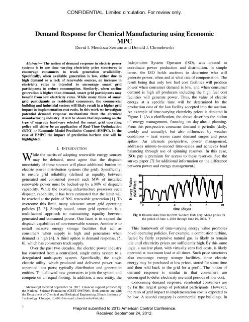
CONFIDENTIAL. Limited circulation. For review only.Demand Response for Chemical Manufacturing using EconomicMPCDavid I. Mendoza-Serrano and Donald J. ChmielewskiAbstract— The notion of demand response in electric powersystems is to use time varying electricity price structures toencourage consumers to track generation availability.Specifically, when available generation is low, either due tohigh demand or a lack of renewable sources, an increase inelectricity rates is intended to encourage smart gridparticipants to reduce consumption. Similarly, when on-linegeneration is higher than demand, smart grid participants maybenefit from low electricity rates. While many think of smartgrid participants as residential consumers, the commercialbuilding and industrial sectors will likely result in a higher gridimpact to implementation cost ratio. In this work we investigatepotential demand response mechanisms from the chemicalmanufacturing industry. It will be shown that depending on thetype of upgrade hardware selected the smart grid operatingpolicy will either be an application of Real-Time Optimization(RTO) or Economic Model Predictive Control (EMPC). In thecase of EMPC the impact of prediction horizon size will behighlighted.WI. INTRODUCTIONhile the merits of adopting renewable energy sourcesmay be debated, most agree that the dispatchuncertainty of these sources will place additional burden onelectric power distribution systems (the grid). Specifically,to ensure grid reliability (defined as equality betweengenerated and consumed power) each MW of installedrenewable power must be backed-up by a MW of dispatchcapability. While the existing infrastructure possesses suchdispatch capability, it has been estimated that the limit willbe reached at the point of 20% renewable generation [1]. Toovercome this limit, many advocate smart grid operatingpolicies [2, 3]. Simply stated, smart grid operation is amultifaceted approach to maintaining equality betweengenerated and consumed power. One facet is to expand thedispatch capabilities of non-renewable sources. Another is toinstall massive energy storage facilities that act asconsumers when supply is high and generators whendemand is high [4]. A third option is demand response, [5,6], which has consumers track supply.Over the past two decades, the electric power industryhas converted from a centralized, single entity system to aderegulated multi-party system. Specifically, the singleelectric utility, which produced and delivered power, wasseparated into parts; typically distribution and generationentities. This allowed new generators to join the system andcompete on an equal footing. In addition, a new entity, theManuscript received September 24, 2012. Financial support provided bythe National Science Foundation (CBET-0967906). Both authors are withthe Department of Chemical and Biological Engineering, Illinois Institute ofTechnology, Chicago, IL 60616 (e-mail: chmielewski@iit.edu).Independent System Operator (ISO), was created tocoordinate power production and distribution. In simpleterms, the ISO holds auctions to determine who willgenerate power, when and at what rate of compensation. Theresult being that only low fuel cost facilities will producepower when consumer demand is low, and when consumerdemand is high all producers including the high fuel costfacilities will generate power. Thus, the value of electricenergy at a specific time will be determined by theproduction cost of the last facility accepted into the auction.An example of time-varying electricity prices is depicted inFigure 1. (As a clarification, the above describes the notionof energy management, focusing on day-ahead planning.From this perspective, consumer demand is periodic (daily,weekly and annually), but also influenced by weatherconditions – heat waves cause demand surges and pricespikes. An alternate perspective, power management,addresses minute-to-second time-scales and achieves loadbalancing through use of spinning reserves. In this case,ISOs pay a premium for access to these reserves. See thesurvey paper [7] for additional information on the differencebetween power and energy management.)Energy Value($/MWhr)403020100 0 2 4 6 8 10time (days)Fig 1: Historic data from the PJM Western Hub, Day-Ahead prices forthe period of June 1, 2001 through June 10, 2001, [8].This framework of time-varying energy value promotesnovel operating policies. For example, a combustion turbine,fueled by fairly expensive natural gas, is likely to remainidle until electricity prices are sufficiently high. By this samelogic, a nuclear plant, with virtually zero fuel costs, is likelyoperated at maximum load at all times. Such price structuresalso encourage energy storage facilities, since electricenergy may be purchased at low prices, stored for some timeand then sold back to the grid for a profit. The notion ofdemand response is similar in that consumers areencouraged to defer electricity use until periods of low cost.Concerning demand response, residential consumers areby far the largest group of potential participants. However,the ratio of grid impact to implementation cost is expected tobe low. A second category is commercial type buildings. In1Preprint submitted to 2013 American Control Conference.Received September 24, 2012.

CONFIDENTIAL. Limited circulation. For review only.these cases, thermal energy storage (either passive or active)is used to time shift the power consumed by the HeatingVentilation and Air Conditioning (HVAC) system, [9-11]. Athird category is industrial consumers, where the populationis relatively small and consumption is large. It should also beclarified that industrial facilities may contribute to both thepower and energy management. In the former, the facilitywill relinquish control to the ISO and act similar to spinningreserves, [12, 13]. The current effort, however, focuses onenergy management and assumes the availability of a timedependentprice structure.The current effort will investigate the implementation ofdemand response at a chemical manufacturing facility. Thenext section will describe possible equipment upgrades thatwill enable demand response from such facilities and showhow the conventional tool of economic based Real-TimeOptimization (RTO) can be expanded to generate a smartgrid operating policy. Section 3 will expand the hardwareupgrade options to include material storage. In this case, thesmart grid operating policy will need to be an application ofEconomic Model Predictive Control (EMPC).In EMPC, the quadratic objective function typically usedin MPC is replaced by an expression directly reflectingrevenue, [14]. Similar approaches have worked well in thearea of HVAC control, [15-20], as well as in processoperations scheduling [20-24]. In both of these applications,computational issues, resulting from the large size of the onlineoptimization problem, have been reported. Efforts toreduce this computational burden, by reducing predictionhorizon, have resulted in undesirable closed-loopcharacteristics, including inventory creep, [23] and bangbangtype actuation [20]. It is also noted that efforts toensure closed-loop stability of the EMPC algorithm haverequired the use of specialized analysis techniques and nonintuitiveadditions to the basic algorithm [25-27].each unit (Q i ). All steam utilities are provided by a steamplant, so the utility cost is the cost of fuel, proportional to thesum of steam utilities.A possible smart grid upgrade is to install electric heatersto supplement steam utility. Given this hardware, electricpower would partially drive process units, which wouldmake sense if electricity price is sufficiently low. Or, onecould install a co-generation plant for simultaneousgeneration of steam and electric power. Such a plant wouldbe useful during periods of high electricity price.Specifically, steam utilities would come from the cogenerationplant and the simultaneously produced electricpower would be sold to the grid. A third option is to installmaterial storage units (S 1 through S 5 ). Suppose unit P 4 is alarge consumer of electric energy. Then, during periods ofhigh electric price this unit could be turned down andmaterial from S 5 could be recovered while material is storedin S 4 . To build up the inventory in S 5 , and eventually use thatin S 4 , the P 4 unit would need a maximum throughput greaterthan the nominal. In this section the first two options will beinvestigated and the third will be addressed in Section 3.To keep the example simple, we will consider only themass flows through and between each unit. (A properanalysis would consider the compositions of each stream aswell.) The mass flow relations for each unit are assumed tobe the following:QQQQ3610130.25Q 0.9Q0.1Q10.583Q81250.3Q 0.8Q29QQQQ7411140.75Q 0.1Q0.9Q810.417Q1250.7Q 0.2QGiven these relations and the process diagram (assuming nostorage), the system has 8 degrees of freedom. As such, wewill define an 8x1 vector, m, as the set of manipulations andarbitrarily select the flows Q 1 , Q 2 , Q 5 , Q 8 , Q 9 , Q 12 , Q 15 , Q 16 to beset equal to the manipulations, the elements of m. Thus, thevector of flows, Q, will be linearly related to themanipulation vector (where ' is determined from (1)):92(1)Q ' m(2)Fig 2: Simplified process diagram of a chemical manufacturing plantII. OPERATION WITH REAL-TIME OPTIMIZATIONTo motivate the discussion, consider the process diagramof Figure 2, which resembles a simplified version of arefinery (for the moment, ignore the storage units S 1 throughS 5 ). Plant profit is defined as the difference between rawmaterial costs and product revenues minus the cost ofutilities. Utilities are required to operate each process unit(P 1 through P 4 ) and the energy required to provide steamutility is roughly proportional to the material flow throughA material balance around each stream (that contains astorage unit in Figure 1) results in the following relations:000Q Q37145Q QQ9Q Q21600Q Q4118Q QQIn vector form, these relations are defined as 0 /Q .Combining (2) and (3) we arrive at the following materialbalance relations for the process:1215(3)0 / ' m(4)2Preprint submitted to 2013 American Control Conference.Received September 24, 2012.

CONFIDENTIAL. Limited circulation. For review only.(The somewhat unconventional development of the abovematerial balances is intended to simplify the developmentsin Section 3.)The energy required by each unit is assumed to beproportional to the material flows into each.ee130.5Q 0.5Q10.5Q 0.5Q829ee240.5Q4Qwhere the proportionality constants have units of GJ/bbl. Invector form, these relations are defined as e * Q . If thisenergy is delivered by steam the conversion efficiency isassumed to be K s = 0.75 and if delivered by electric heatersthen the efficiency is assumed to be K e = 0.95. In vectorform, these relations are defined as e 4ses 4eee, where4 K s I , 4 I and e s and e e are vectors indicating these K eenergy sent to each unit via steam and electricity,respectively. In summary, the energy balances at each unitare defined as:ssee125(5)*Q 4 e 4 e(6)If the steam utility is produced from a dedicated steamplant, then the efficiency of converting fuel energy, f sp , tosteam energy is assumed to be K sp = 0.75 (GJ steam/GJ fuel).If steam is produced from a co-generation plant, then theefficiency of converting fuel energy, f cog , to steam isassumed to be K cogs = 0.50. However, if steam is producedfrom the co-generation plant, then electricity must also beproduced at an efficiency of K coge = 0.15f spf cogSteam PlantCo-GenerationPlantSteamBanke gElectricNodee s1es2e s3e s4Fig 3: Simplified process diagram of utility flowse e1ee2e e3e e4An energy balance around the steam bank of Figure 3results in the following relation:K f K f 1e(7)spspcogscogswhere 1 is a 1x4 row vector of ones. An energy balancearound the electric node of Figure 3 results in the followingrelation:e K f 1e(8)gcogecogewhere e g is the energy taken from the grid. (If negative, thenthis magnitude of energy would be supplied to the grid.)Concerning operating limitations; all process flows mustbe positive ( Q 'm t 0 , e t 0 ), all electricity must flowinto the process units must be positive (st 0 ), and fuelenergy into the steam and co-generation plants must bepositive ( f t 0 and t 0 ). It is highlighted that there isspf cogno limitation on the amount of electric energy taken from orsent to the grid. Finally, each unit will have limitations withrespect to total input:Q Qd u182Q Qd umax19max1max3max2Q d uQ512d umax2max4max3u 1.5 , u 0. 727 , u 1. 075 and 1. 2(all in bbl/sec)Price ofElectricity ($/GJ))Fuel Energy toSteam Plant (GJ/secFuel Energy t oCo-GenerationPlant (GJ/sec)Power from Grid(GJ/sec)Instantan iousProfit ($/sec)105Fig 4. Price of Electricitye eFig 5. Consumer loads for Example 1maxu 400 0.5 1 1.5 2time (days)10500 0.5 1 1.5 2time (days)15105The econom ic aspects of the process are as follows: Thecost raw material, Q 1 , is $100/bbl. The value of the product(9)00 0.5 1 1.5 2time (days)420-20 0.5 1 1.5 2time (days)504030200 0.5 1 1.5 2time (days)3Preprint submitted to 2013 American Control Conference.Received September 24, 2012.

CONFIDENTIAL. Limited circulation. For review only.streams (Q 6 , Q 10 , Q 13 , Q 15 , Q 16 ) is (200, 120 35, 50, 100) $/bbl.The cost of fuel (to both the steam and co-generation plants)is c f = $3/GJ. (This is comparable to the cost of natural gas~$3/MMBTU). The cost of electricity is assumed to be c e =$5.5/GJ (This is comparable to a constant tariff rate of$20/MWhr.)In summary, the real-time optimization problem aimed atmaximizing instantaneous operating profit is defined as:maxmt0,Q t0,est0,eet0,fspt0,fcogt0,eg^cQQ cffsp cs.t. (2), (4), (6), (7), (8),(9)(10)The solution to problem (10) is summarized as: Q = [0.9580.541 0.727 0.773 0.727 0.424 0.301 0.773 0.302 0.4730.602 0.602 0.602 0.541 0.0 0.0] T bbl/sec, e s = [1 0.4850.717 3.21] T GJ/sec, e s = 0, f sp = 7.21 GJ/sec, f cog = 0 and e g= 0. Basically, the plant is operated using only energy fromthe steam plant. The profit resulting from this set ofoperating conditions is 26.3 $/sec. To provide additionalcontext, the energy cost is 21.7 $/sec. This indicates that aceiling to instantaneous profit (resulting from zero energycosts) is $48.0/sec. It is also noted that a feed of 0.958bbl/sec is about 84,000 bbl per day.Now consider the case of a time varying electricity price.To facilitate analysis of the results, the perfect sine wave ofFigure 4 will be used as the price of electricity. Note that thecurve average is 5.5 $/GJ, the sine wave has an amplitude of4.2 $/GJ and a period of 1day. The curve is also sampled at 1hour periods. The solution to problem (10) at each timeperiod is depicted in Figure 5 and results in RTO operationas one would expect. During the first few sample periods(when the price of electricity is close to 5.5 $/GJ), allutilities are provided by the steam plant. Then as the price ofelectricity rises (past about 7 $/GJ), the steam plant is turnedoff and the co-generation plant is turned on. The amount ofsteam produced from co-generation is exactly enough tomeet the energy needs of the process units and all theproduced electricity is sent to the grid to generate revenuefor the plant (since this electricity has high value at thattime). The resulting increase in instantaneous profit isobserved during the 0.1 - 0.5 day time period. Then, as theprice of electricity drops the co-generation plant is turned offand the steam plant is turned on very briefly (for about 2hours at about 0.5 days). Once the price of electricitysufficiently drops (below about 4.5 $/GJ), the steam plant isturned off and the electric heaters are turned on. The amountof energy taken from the grid is exactly the amount neededto meet the energy needs of the process units. Since thisenergy is being received at very low cost (due to the lowprice of electricity during this period) the instantaneousprofit of the plant approaches the ceiling value of 48 $/sec,and would surpass this value if the price where to becomenegative (which is not impossible). Finally, operation duringffcog c eeg`the second day is identical to the first. It is also important tonote that the material flows remained constant for all time(equal to the baseline values of the previous paragraph). Theaverage profit over the 2 day period was found to be 32.3$/sec a 22.8% increase over the baseline case.III. OPERATION WITH ECONOMIC MPCWe now consider th e case of adding the storage unitsdepicted in Figure 2. The first step to adding energy storageto the model is to add a time index (k) to all of the processvariables. (Actually, this indexing occurred implicitly in theprevious section, but we just did not discuss it.) Next, definethe amount of material in each of the storage units (at time k)by the 5 elements of a vector M(k). Then, Equation (4) isreplaced with the following:whereM ( k 1)M ( k) ' ts /'m(k)0 d M ( k)d Msmax(11)' t is the sample period (= 1 hour). Finally, theEMPC optimization problem is define by changing theobjectivefunction from instantaneous profit to averageprofit:N 1°­ 1 °½max ® ¦ pinst( k)¾m( k)t0,Q ( k)t0,( ) 0, ( ) 0,°¯N0 °e k t e k t ks e¿(12)fsp( k)t0,fe ( k)gcog( k)t0,s.t. (2), (11),(6), (7),(8),(9)where p ( k)c Q ( k) c f ( k) c f ( k) c ( k)e ( k)instQ f sp f cog e g .This optimization problem is implemented within areceding horizon framework (the current state of theinventories is set equal to M(0) and only the first time indexof the solution is input to the process). This mapping fromM(0) to the manipulated variables is denoted as the EMPCpolicy. It is highlighted that this mapping is also a functionof the forecasted price of electricity (k), k = 0 ... N-1. Onthe subject of forecasting, the following simulations willassume perfect forecasting in the sense that all future pricesare known to the EMPC. (Extension to the imperfectforecasting case can be found in [28]).As one would expect application of the EMPC with M max= [0 0 0 0 0] T results in operation identical to the RTOcase regardless of the value selected for the predictionhorizon, N. However, application of EMPC with M max = [00 0 10000 10000] T bbl and N = 48 (a 2 day predictionhorizon) results in the plots of Figure 6. The curves aresimilar to the RTO case but a bit more exaggerated. The firstplot shows that unit 4 is off during the first few hours. Thisis made possible by drawing from the inventory in storage 5and adding to the inventory in storage 4 (see the secondplot). This allows the rate of fuel to the steam plant to bereduced (third plot). Due to this reduction in fuel usage, thec e4Preprint submitted to 2013 American Control Conference.Received September 24, 2012.

CONFIDENTIAL. Limited circulation. For review only.instantaneous profit increases during this period. Then, asthe price of electricity increases (after 0.1 days) the cogenerationplant is turned on (and the steam plant is turnedoff). In contrast to the RTO case, additional fuel is set to theco-generation plant to provide the steam energy necessary toincrease the throughput of unit 4, beyond its nominalthroughput. (Note that the maximum throughput of unit 4was defined to be 2 times the throughput of the baselinecase.) Due to this increase in fuel to the co-generation plantadditional electric energy is produced and sold to the grid (atthe high prices of the period). Due to the large amount offuel used by the co-generation plant, instantaneous profit islow during this period, but the inventory in 5 has beenreplenished. Then, as electricity prices decrease (to around5.5 $/GJ), unit 4 is turned off for about 6 hours, until M 4 isfull and M 5 is empty. At about 0.6 days, both steamgenerators are turned off and the plant is run purely off ofcheap electricity. This included the period from about 0.7 to0.9 when unit 4 is run at greater than nominal throughput.Notice that during this period of high unit 4 throughput, theinstantaneous profit hardly decreases at all, compared to theRTO case. The simulation of Figure 6 can be summarized asfollows: The EMPC policy calls for high throughput at unit4; when electric energy is cheap to buy (0.7-09) or when thesale of high value electric energy will off-set the throughputcosts (0.2-0.4). The average profit for the EMPC case(determined over a 20 day simulation) is 34.2 $/sec, which isa 30.0% increase over the baseline and 7.2 percentage pointshigher than the RTO case.It should be highlight that in the simulation of theprevious paragraph the storage units M 4 and M 5 were initialcharged with 5000 bbl of inventory (see the initial points ofthe second plot of Figure 6). If this initial charge was notpresent then the EMPC would call on the other parts of theprocess to change, somewhat radically, to create suchinventories, which would then allow unit 4 to respondsimilarly to that of Figure 6. A fairly small example of thisredistribution can be observed in the top plot of Figure 6.Here we see that Q 1 initially drops slightly below its nominalvalue. What is happening is that the EMPC feels that there isa little too much material in the storage units, so it reduces Q 1to get the inventory in the optimal position. This sort ofresponse is expected to be much more frequent and severe ifwe were to replace the sine wave cost of electricity with theirregularities of true forecasts.Figure 7 illustrates the impact of reducing the predictionhorizon to 6 hours. In the top it is observed that the averageinventory of both tanks is dropping. This can also beobserved by the two drops in Q 1 (at 0.0, 0.2 and 1.0 days),indicating that the EMPC feels that it would be morebeneficial to convert this material in storage and sell itthrough streams 6 and 10. This is a classic example ofinventory creep. It is obvious that the abbreviated horizon ofthis EMPC is the source of this poor behavior. Specifically,the EMPC is short sighted (or as stated in [23] ‘myopic’) inthe sense that it is taking the short term gains rather thanwaiting to obtain the down the road benefits. A simulation ofthis EMPC over 50 days resulted in the inventory eventuallygoing to very close to zero and a policy almost identical tothe RTO case. It is also noted that a similar long timesimulation with the 48 hour horizon EMPC, resulted in asustained level of inventory.Mass inStorage (bbl)Mass Flow(bbl/sec)21Q 1Q 12Q 13Q 1400 0.5 1 1.5time (days)15000100005000)Fuel Energy toSteam Plant (GJ/secFuel E nerg y toCo-GenerationPlant (GJ/sec)Power from Grid(GJ/sec)InstantaniousProfit ($/sec)00 0.5 1 1.5 2time (days)105Fig 6. Comparison of RTO and EMPC with a 48 hour prediction horizonIV. CONCLUSIONSM 4M 5RTOEMPC00 0.5 1 1.5 2time (days)2010RTOEMPC00 0.5 1 1.5 2time (days)8642RTOEMPC0-2-40 0.5 1 1.5 2time (days)504030RTOEMPC200 0.5 1 1.5 2time (days)I n this work we have illustrated the potential opportunities ofsmart grid operation within a chemical manufacturingfacility. Th e provided example indicated as much as a 30%increase in operating profits. However, it is important toemphasize that this increase in operating profit was enableby the installation of new hardware (electric heaters, a cogenerationplant, material storage units and a doubling of thethroughput capabilities of one of the processing units). To5Preprint submitted to 2013 American Control Conference.Received September 24, 2012.

CONFIDENTIAL. Limited circulation. For review only.arrive at a proper economic assessment of the smart gridopportunity one must factor in the cost of this upgradeequipment. The methods of [29, 30] illustrate one approachto this combined capital and operating cost analysis.It was also observed that economic performance is astrong function of EMPC horizon size. While the 48 hourhorizon presented little computational challenge in the smallexample of this paper, it is likely to be a challenge in morerealistic examples where the model is substantially largerand additional constraints (ramp rate limitations and start-up/ shut-down restrictions) are imposed. In these cases, themethod of infinite-horizon EMPC, [20, 28], will likely ofutility.(bbl)Ma ss inStorage100005000M 4M 500 0.5 1 1.5 2time (days)[11] Roth, K., R. Zogg, and J. Brodrick (2006) Cool ThermalEnergy Storage, ASHRAE Journal., 48, pp 94-96[12] Parvania, M., M.Fotuhi-Firuzabad (2010). Demand response1(1)scheduling by stochastic SCUC. IEEE Trans. Smart Grid,89-98.[13] Nguyen, D.T., M. Negnevitsky, M. de Groot (2011). Poolbaseddemand response exchange – concept and modeling.IEEE Trans. Power Systems,26(3), pp 1677-1685.[14] Rawlings, J.B. and R. Amrit (2009) Optimizing processeconomic performance using model predictive control,Nonlinear Model Predictive Control, Lecture Notes in Controland Information Sciences, Vol. 384, pp 119-138[15] Braun, J.E. (1992) A comparison of chiller-priority, storage-priority, and optimal control of an ice-storage system,ASHRAE Trans., vol. 98(1), pp 893-902[16] Morris, F.B., J.E. Braun and S.J. Treado (1994) Experimentaland simulated performance of optimal control of buildingthermal storage, ASHRAE Trans., vol. 100(1), pp 402-414[17] Kintner-Meyer, M. and A.F. Emery (1995) Optimal control ofan HVAC system using cold storage and building thermalcapacitance, Energy and Buildings, vol. 23, pp 19-31[18] Henze, G.P., M. Krarti, M.J. Brandemuehl (2003) Guidelinesfor improved performance of ice storage systems, Energy andBuildings, vol. 35, pp 111-1272[19] Braun, J.E. (2007) Impact of control on operating costs forQ Q 1 12cool storage systems with dynamic electric rates, ASHRAE1Trans., vol. 113(2), pp343-354[20] Mendoza-Serrano, D.I. and D.J. Chmielewski (2012) Infinite-0horizon Economic MPC for HVAC systems with Active0 0.5 1 1.5Thermal Energy Storage, Proc. of the Conf. Dec. Contr.,time (days)Honolulu, HI (in press)Fig 7. EMPC with a 6 hour prediction horizon[21] Karwana, M.H. and M.F. Keblisb (2007) Operations planningwith real time pricing of a primary input, Comp. Oper. Res.,vol. 34, pp 848–867REFERENCES[22] Baumrucker, B.T. and L.T. Biegler (2010) MPEC strategiesfor cost optimization of pipeline operations, Comp. Chem.[1] Lindenberg, S., Smith, B., O’Dell, K., DeMeo, E., Ram, B.Eng., vol. 34, pp 900– 913(2008) 20% Wind Energy by 2030: Increasing Wind Energy’s [23] Lima, R.M., I.E. Grossmann and Y. Jiao (2011) Long-termContribution to U.S. Electric Supply. DOE/GO-102008-2567 scheduling of a single-unit multi-product continuous process[2] Farhangi, H. (2010) The path of the smart grid, IEEE Power to manufacture high performance glass, Comp. Chem. Eng.,and Energy Magazine, 8(1), pp.18-28vol. 35(3), pp 554–574[3] Ipakchi, A., F. Albuyeh (2009) Grid of the future," IEEE [24] Kostina, A.M., G. Guillén-Gosálbeza, F.D. Meleb, M.J.Power and Energy Magazine, 7(2), pp.52-62Bagajewiczc, L. Jiméneza (2011) A novel rolling horizon[4] Chen, H., T.N. Cong, W. Yang, C. Tan, Y. Li, Y. Ding (2009). strategy for the strategic planning of supply chains:Progress in electrical energy storage system: a critical review.Application to the sugar cane industry of Argentina, Comp.Progress in Natural Science, 19, pp 291-312.Chem. Eng., vol. 35, pp 2540– 2563[5] Rahimi, F., A. Ipakchi (2010) Demand response as a market [25] Diehl, M., R. Amrit and J.B. Rawlings (2011) A Lyapunovresource under the smart grid paradigm, IEEE Trans. Smart function economic optimizing model predictive control, IEEEGrid, 1(1), pp.82-88Trans. Aut. Contr. Vol 56(3), pp 703-707[6] Walawalkar, R., S. Fernands, N. Thakur, K.R. Chevva (2010) [26] Huang, R. and L. Biegler (2011) Stability of economicallyorientedNMPC with periodic constraint, Preprints of 18thEvolution and current status of demand response (DR) inelectricity markets: Insights from PJM and NYISO, Energy, IFAC World Congress, Milano, Italy, pp 10499- 1050435(4), pp 1553-1560[27] Heidarinejad, M., J. Liu, P.D. Christofides (2012) Economic[7] Soroush, M.; D.J.Chmielewski, (2012) Process systemsmodel predictive control of nonlinear process systems usingopportunities in power generation, storage and distribution,Lyapunov techniques, AIChE J., vol 58, pp. 855–870Comp. Chem Eng., in press.[28] Omell, B.P.; D.J. Chmielewski (2012) IGCC Power Plant[8] PJM (2012) PJM Day-Ahead Historical Data:Dispatch Using Infinite-Horizon Economic Model Predictivehttp://www.pjm.com/markets-and-operations/energy/dayahead/day-ahead-historical.aspx(accessed on March 30, 2012) [29] Yang, M.W., B.P Omell and D.J. Chmielewski (2012)Control, Ind Eng. Chem. Res, submitted.[9] House, J.M., and T.F. Smith (1995) Optimal control ofController design for dispatch of IGCC power plants, Proc.building and HVAC systems, Proc. of the Am Cont. Conf,Am. Contr. Conf., Montreal, CanadaSeattle, WA, pp 4326-4330.[30] Mendoza-Serrano, D.I. and D.J. Chmielewski (2012)[10] Chen, H-J., D.W. Wang, S-L. Chen (2005) Optimization of an Controller and system design for HVAC with Thermal Energyice-storage air conditioning system using dynamicStorage, Proc. of the Am. Cont. Conf., Montreal, Canadaprogramming method, App. Thermal Eng., vol. 25, pp 461-472Mass Flow(bbl/sec)6Preprint submitted to 2013 American Control Conference.Received September 24, 2012.