Demand Response for Chemical Manufacturing using Economic MPC

More documents

Recommendations

Info

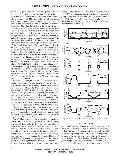
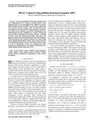
CONFIDENTIAL. Limited circulation. For review only.streams (Q 6 , Q 10 , Q 13 , Q 15 , Q 16 ) is (200, 120 35, 50, 100) $/bbl.The cost of fuel (to both the steam and co-generation plants)is c f = $3/GJ. (This is comparable to the cost of natural gas~$3/MMBTU). The cost of electricity is assumed to be c e =$5.5/GJ (This is comparable to a constant tariff rate of$20/MWhr.)In summary, the real-time optimization problem aimed atmaximizing instantaneous operating profit is defined as:maxmt0,Q t0,est0,eet0,fspt0,fcogt0,eg^cQQ cffsp cs.t. (2), (4), (6), (7), (8),(9)(10)The solution to problem (10) is summarized as: Q = [0.9580.541 0.727 0.773 0.727 0.424 0.301 0.773 0.302 0.4730.602 0.602 0.602 0.541 0.0 0.0] T bbl/sec, e s = [1 0.4850.717 3.21] T GJ/sec, e s = 0, f sp = 7.21 GJ/sec, f cog = 0 and e g= 0. Basically, the plant is operated using only energy fromthe steam plant. The profit resulting from this set ofoperating conditions is 26.3 $/sec. To provide additionalcontext, the energy cost is 21.7 $/sec. This indicates that aceiling to instantaneous profit (resulting from zero energycosts) is $48.0/sec. It is also noted that a feed of 0.958bbl/sec is about 84,000 bbl per day.Now consider the case of a time varying electricity price.To facilitate analysis of the results, the perfect sine wave ofFigure 4 will be used as the price of electricity. Note that thecurve average is 5.5 $/GJ, the sine wave has an amplitude of4.2 $/GJ and a period of 1day. The curve is also sampled at 1hour periods. The solution to problem (10) at each timeperiod is depicted in Figure 5 and results in RTO operationas one would expect. During the first few sample periods(when the price of electricity is close to 5.5 $/GJ), allutilities are provided by the steam plant. Then as the price ofelectricity rises (past about 7 $/GJ), the steam plant is turnedoff and the co-generation plant is turned on. The amount ofsteam produced from co-generation is exactly enough tomeet the energy needs of the process units and all theproduced electricity is sent to the grid to generate revenuefor the plant (since this electricity has high value at thattime). The resulting increase in instantaneous profit isobserved during the 0.1 - 0.5 day time period. Then, as theprice of electricity drops the co-generation plant is turned offand the steam plant is turned on very briefly (for about 2hours at about 0.5 days). Once the price of electricitysufficiently drops (below about 4.5 $/GJ), the steam plant isturned off and the electric heaters are turned on. The amountof energy taken from the grid is exactly the amount neededto meet the energy needs of the process units. Since thisenergy is being received at very low cost (due to the lowprice of electricity during this period) the instantaneousprofit of the plant approaches the ceiling value of 48 $/sec,and would surpass this value if the price where to becomenegative (which is not impossible). Finally, operation duringffcog c eeg`the second day is identical to the first. It is also important tonote that the material flows remained constant for all time(equal to the baseline values of the previous paragraph). Theaverage profit over the 2 day period was found to be 32.3$/sec a 22.8% increase over the baseline case.III. OPERATION WITH ECONOMIC MPCWe now consider th e case of adding the storage unitsdepicted in Figure 2. The first step to adding energy storageto the model is to add a time index (k) to all of the processvariables. (Actually, this indexing occurred implicitly in theprevious section, but we just did not discuss it.) Next, definethe amount of material in each of the storage units (at time k)by the 5 elements of a vector M(k). Then, Equation (4) isreplaced with the following:whereM ( k 1)M ( k) ' ts /'m(k)0 d M ( k)d Msmax(11)' t is the sample period (= 1 hour). Finally, theEMPC optimization problem is define by changing theobjectivefunction from instantaneous profit to averageprofit:N 1° 1 °½max ® ¦ pinst( k)¾m( k)t0,Q ( k)t0,( ) 0, ( ) 0,°¯N0 °e k t e k t ks e¿(12)fsp( k)t0,fe ( k)gcog( k)t0,s.t. (2), (11),(6), (7),(8),(9)where p ( k)c Q ( k) c f ( k) c f ( k) c ( k)e ( k)instQ f sp f cog e g .This optimization problem is implemented within areceding horizon framework (the current state of theinventories is set equal to M(0) and only the first time indexof the solution is input to the process). This mapping fromM(0) to the manipulated variables is denoted as the EMPCpolicy. It is highlighted that this mapping is also a functionof the forecasted price of electricity (k), k = 0 ... N-1. Onthe subject of forecasting, the following simulations willassume perfect forecasting in the sense that all future pricesare known to the EMPC. (Extension to the imperfectforecasting case can be found in [28]).As one would expect application of the EMPC with M max= [0 0 0 0 0] T results in operation identical to the RTOcase regardless of the value selected for the predictionhorizon, N. However, application of EMPC with M max = [00 0 10000 10000] T bbl and N = 48 (a 2 day predictionhorizon) results in the plots of Figure 6. The curves aresimilar to the RTO case but a bit more exaggerated. The firstplot shows that unit 4 is off during the first few hours. Thisis made possible by drawing from the inventory in storage 5and adding to the inventory in storage 4 (see the secondplot). This allows the rate of fuel to the steam plant to bereduced (third plot). Due to this reduction in fuel usage, thec e4Preprint submitted to 2013 American Control Conference.Received September 24, 2012.
CONFIDENTIAL. Limited circulation. For review only.instantaneous profit increases during this period. Then, asthe price of electricity increases (after 0.1 days) the cogenerationplant is turned on (and the steam plant is turnedoff). In contrast to the RTO case, additional fuel is set to theco-generation plant to provide the steam energy necessary toincrease the throughput of unit 4, beyond its nominalthroughput. (Note that the maximum throughput of unit 4was defined to be 2 times the throughput of the baselinecase.) Due to this increase in fuel to the co-generation plantadditional electric energy is produced and sold to the grid (atthe high prices of the period). Due to the large amount offuel used by the co-generation plant, instantaneous profit islow during this period, but the inventory in 5 has beenreplenished. Then, as electricity prices decrease (to around5.5 $/GJ), unit 4 is turned off for about 6 hours, until M 4 isfull and M 5 is empty. At about 0.6 days, both steamgenerators are turned off and the plant is run purely off ofcheap electricity. This included the period from about 0.7 to0.9 when unit 4 is run at greater than nominal throughput.Notice that during this period of high unit 4 throughput, theinstantaneous profit hardly decreases at all, compared to theRTO case. The simulation of Figure 6 can be summarized asfollows: The EMPC policy calls for high throughput at unit4; when electric energy is cheap to buy (0.7-09) or when thesale of high value electric energy will off-set the throughputcosts (0.2-0.4). The average profit for the EMPC case(determined over a 20 day simulation) is 34.2 $/sec, which isa 30.0% increase over the baseline and 7.2 percentage pointshigher than the RTO case.It should be highlight that in the simulation of theprevious paragraph the storage units M 4 and M 5 were initialcharged with 5000 bbl of inventory (see the initial points ofthe second plot of Figure 6). If this initial charge was notpresent then the EMPC would call on the other parts of theprocess to change, somewhat radically, to create suchinventories, which would then allow unit 4 to respondsimilarly to that of Figure 6. A fairly small example of thisredistribution can be observed in the top plot of Figure 6.Here we see that Q 1 initially drops slightly below its nominalvalue. What is happening is that the EMPC feels that there isa little too much material in the storage units, so it reduces Q 1to get the inventory in the optimal position. This sort ofresponse is expected to be much more frequent and severe ifwe were to replace the sine wave cost of electricity with theirregularities of true forecasts.Figure 7 illustrates the impact of reducing the predictionhorizon to 6 hours. In the top it is observed that the averageinventory of both tanks is dropping. This can also beobserved by the two drops in Q 1 (at 0.0, 0.2 and 1.0 days),indicating that the EMPC feels that it would be morebeneficial to convert this material in storage and sell itthrough streams 6 and 10. This is a classic example ofinventory creep. It is obvious that the abbreviated horizon ofthis EMPC is the source of this poor behavior. Specifically,the EMPC is short sighted (or as stated in [23] ‘myopic’) inthe sense that it is taking the short term gains rather thanwaiting to obtain the down the road benefits. A simulation ofthis EMPC over 50 days resulted in the inventory eventuallygoing to very close to zero and a policy almost identical tothe RTO case. It is also noted that a similar long timesimulation with the 48 hour horizon EMPC, resulted in asustained level of inventory.Mass inStorage (bbl)Mass Flow(bbl/sec)21Q 1Q 12Q 13Q 1400 0.5 1 1.5time (days)15000100005000)Fuel Energy toSteam Plant (GJ/secFuel E nerg y toCo-GenerationPlant (GJ/sec)Power from Grid(GJ/sec)InstantaniousProfit ($/sec)00 0.5 1 1.5 2time (days)105Fig 6. Comparison of RTO and EMPC with a 48 hour prediction horizonIV. CONCLUSIONSM 4M 5RTOEMPC00 0.5 1 1.5 2time (days)2010RTOEMPC00 0.5 1 1.5 2time (days)8642RTOEMPC0-2-40 0.5 1 1.5 2time (days)504030RTOEMPC200 0.5 1 1.5 2time (days)I n this work we have illustrated the potential opportunities ofsmart grid operation within a chemical manufacturingfacility. Th e provided example indicated as much as a 30%increase in operating profits. However, it is important toemphasize that this increase in operating profit was enableby the installation of new hardware (electric heaters, a cogenerationplant, material storage units and a doubling of thethroughput capabilities of one of the processing units). To5Preprint submitted to 2013 American Control Conference.Received September 24, 2012.
Page 1 and 2: CONFIDENTIAL. Limited circulation.
Page 3: CONFIDENTIAL. Limited circulation.

Demand Response for Chemical Manufacturing using Economic MPC

You also want an ePaper? Increase the reach of your titles

Delete template?

Save as template?