Fourier Series

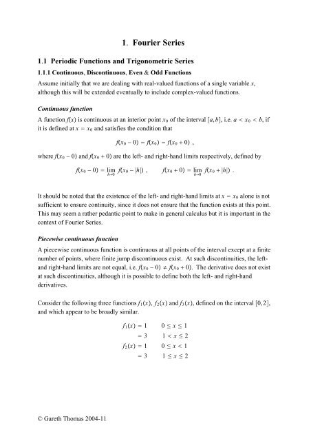
f 3 x 1 0 ≤ x 1 3 1 x ≤ 2Using the definitions of continuity and piecewise continuity given above: all three arecontinuous throughout 0,2, except at x 1 where each is piecewise continuous.Furthermore, the discontinuity at x 1 means that the integral of each function over 0,2is obtained by summing the contributions from 0,1 and 1,2, i.e.valid for m 1,2,3.02fm x dx 01fm x dx 12fm x dx 011 dx 123 dx 4The difference between the functions occurs at x 1 and it is seen that f 1 1 1,f 2 1 3but f 3 1 is not defined. This identifies an important point about discontinuous functions:they may or may not be defined at the point of discontinuity.A restriction is now imposed to ensure that only intervals of a certain type are allowable. Itis assumed that the functions are defined upon a closed interval of the real axis −a,a, anopen interval of the real axis −a,a or the infinite interval −,; the key requirement isthat the interval possesses x 0 as its centre point. The definitions are presented in termsof the closed interval but clearly hold for symmetric intervals that are open or infinite.Even functionAn even function is defined for all x ∈ −a,a to possess the property thatfx f−x .Thus the function is symmetric about the y-axis; one example is fx x 2 and another isfx cosx.Odd functionAn odd function is defined for all x ∈ −a,a to possess the property thatfx − f−x .Thus the function is anti-symmetric about the y-axis; one example is fx x 3 and anotheris fx sinx.These definitions do not impose conditions upon the behaviour of the function at thecentre-point x 0. If continuity is sought, this does not introduce any implications for aneven function beyond the basic property f0 − 0 f0 f0 0 but an odd function can2

only be continuous if fx 0 and this is satisfied by both of the two examples. If x 0ispermitted to be a point of discontinuity, then an odd function may possess a jumpdiscontinuity at this point but the left-hand and right-hand limits are not arbitrary and mustsatisfy the requirement that the function is odd.CombinationsThe concept of evenness and oddness plays an important role in the way that we understandfunctions. Any function on −a,a can be written as the sum of an odd and an evenfunction in a very simple way,fx 1 fx fx2 1 fx f−x 2 1fx − f−x2 Even function Odd function .Example 1Consider fx e x defined upon −a,a. Using the description abovefx 1 fx f−x 2 1fx − f−x2 e x 1 2 ex e −x 1 2 ex − e −x coshx sinhxand we already know that the hyperbolic functions coshx and sinhx are even and oddrespectively.Example 2Suppose that fx and gx are an even and odd function respectively on −a,a and may becontinuous or piecewise continuous, thena−afx gx dx 0.Write the integral asa−afx gx dx 0−afx gx dx 0afx gx dx I 1 I 2 .Then3

I 1 0−afx gx dx a0f−u g−u d−u where x −u 0af−u g−u du on simplification.But f−u fu as it is an even function and g−u −gu as it is an odd function, thusI 1 − 0afu gu du − I2 ,and this proves the result. Note that is a very general result and not dependent uponparticular forms for fx and gx.1.1.2 Periodic FunctionsA real-valued function fx is periodic if it is defined for all x and there is a real number Lsuch thatfx L fxfor all x. The number L is called aperiodof fx. IfL 0 is the smallest non-zero suchnumber , then L 0 is called the period of fx.Figure 1.1.1. A generic periodic function.Clearly fx fx L 0 fx 2L 0 fx 3L 0 ... fx nL 0 ... when L 0 isthe period and n is an integer 2L 0 ,3L 0 , ... ,nL 0 , ... are periods as well. This is clearlyseen in figure 1.1.1.If fx and gx both have the same period L 0 , then the function hx defined by4

hx Afx Bgx ,for constants A and B, will also have the period L 0 . This may seem to be a trivial result butit is not; it shows how an infinite number of periodic functions may be constructed fromjust two periodic functions. Thus for any period L 0 , there will be an infinite number offunctions with this period and the properties of a two-term expression will be carried overto a longer sum or one of infinite length.10.5-1-0.5000.51x-0.5-1y =f(x)y = g(x)Figure 1.1.2(a). The functions fx x 2 and gx x 3 .We can also approach periodic functions from another viewpoint. Suppose that thefunction fx is only defined on −1,1 and that it is well-behaved on this interval. Notethat for the moment, this is restricted to the open interval −1,1 rather than the closedinterval −1,1; the reason for this will become apparent shortly. As an example considerthe two functions fx x 2 and gx x 3 , shown in figure 1.1.2(a), and which were givenas examples of even and odd functions earlier.The two functions can be extended to −, by defining two new functions to coincidewith fx and gx on −1,1 and to be periodic with period 2, shown in figures 1.1.2(b) and5

1.1.2(c) respectively.10.80.60.40.2-100132xFigure 1.1.2(b). The function fx x 2 as a periodic function.It is clear from figure 1.1.2(b) that the periodic form of fx x 2 is a continuous function;it also possesses continuous derivatives everywhere except at x 2m 1, for integer m,where the derivative is discontinuous and changes from a value of 2 to−2 asx increases.In contrast, figure 1.1.2(c) shows that gx x 3 is a piecewise continuous function on anyfinite interval of length greater than 2 and may be continuous or piecewise continuous onany shorter interval. The function gx is discontinuous at all points where x 2m 1,for integer m, and furthermore, it is not defined at these points. This example shows clearlyhow a function initially defined on a finite interval, which is continuous and possibly withcontinuous derivatives, may become discontinuous when extended by periodicity to aninfinite interval and may also introduce points where the function is not defined. However,such properties do not usually cause a problem, provided that the number of points at whicha function is not defined in a period is finite.6

The two may be summarised as follows:f Og |f||g|f og |f||g|→ A as x → x 0→ 0 asx → x 0and note that the equality sign is employed to make the comparison.Example 1The Taylor Series for sinx about x 0issinx x −x33!x55!−x77! ....It can be shown that this series converges for all x, although interest is targeted here to theimmediate vicinity of x 0 since the requirement is to estimate the magnitude of the termsin the series. Using the definitions directly, possible representations of the series aresinx x − Oxx33!x55!−x77! ... x −x33! Ox 5 x −x33! ox 4 and others can be employed as well. If the series is approximated by a set number of terms,then the notation enables an estimate to be made of the qualitative error that occurs.Example 2Consider the function fx x x 2 defined on 0,. At the endpoints of this range, thebehaviour of the function isx x 2 Ox 2 as x → Ox as x → 0and the notation identifies the dominant term in each case. No effort is made to provide abetter estimate and there are an infinite number of functions whose behaviour is Ox 2 asx → and similar remarks apply to the behaviour at the lower limit.Example 3Determine the derivative of fx x 4 .The definition of the derivative of a function fx at a particular value of x is given by9

dfdx limx→0fx x − fxx,which is employed to obtain the derivative by evaluation for the case fx x 4 . Followthis approach and for the given fx,fx x x 4 4x 3 x Ox 2 ,noting that the Ox 2 term, which does do not have to be evaluated, contains all of theunspecified terms of the expansion. Upon substitutionfx x − fxx 4x3 x Ox 2 x 4x 3 Oxand the usual result is obtained by taking the limit as x → 0.The notation is also employed in other fields of mathematics and numerical computation isone of the most important, where the method of application is slightly different but thenotation again provides both approximation and precision to estimate quantities in anintuitive way. Suppose that T is the time taken to perform a particular algorithm and thiscan depend upon the number of time steps, grid points or numerical evaluations associatedwith the algorithm. Then T is often considered to estimated by Tn, wheren representswhichever of the quantities is deemed to be most important and numerical analysts oftenclassify algorithms by Tn On and where (usually integer) is to be determined.10

1.2 Fourier SeriesSuppose a function fx is periodic with period 2 and which we consider to be defined on−,. Can we represent or approximate fx by a trigonometric polynomial (1.1.1) or aseries (1.1.2) on this interval? If so, how do we determine the coefficient set? Again, onlythe series will be considered and the polynomial approximation will be dealt with at a laterpoint.Thus we writefx ~ Sx 1 2 a 0 ∑n1a n cosnx b n sinnx . (1.2.1)Notation: We cannot write fx Sx, asfx can be piecewise continuous, whereas theseries is comprised of continuous functions and so will be continuous provided that itconverges. The symbol ~ means "goes like" and is intended to denote equality at points ofcontinuity and convergence to a known value at points of discontinuity. It should also bepointed out that this does not exclude divergent series.Integrate both sides of (1.2.1) over the whole interval −, and assume that term-by-termintegration is allowable,−fx dx −12 a 0 ∑n1a n cosnx b n sinnxdx 1 2 a 0 2 a 0 a 0 1 −fx dx (1.2.2)where the results −cosnx dx −sinnx dx 0 when n 0 have been used.To find the a n s, multiply both sides of (1.2.1) by cosmx, wherem is a fixed positiveinteger, and integrate over −,,−fxcosmx dx −∑n1 ∑n1−a n −12 a 0 ∑n1a n cosnx b n sinnxa n cosnxcosmx b n sinnxcosmxcosnxcosmx dx ∑n1cosmx dxdxb n sinnxcosmx dx−Similarly11

−fxsinmx dx ∑ a n −n1cosnxsinmx dx ∑n1b n sinnxsinmx dx.−These expressions contain integrals like−cosnxcosmx dx, cosnxsinmx dx and− sinnxsinmx dx.−They are usually evaluated using either addition formulae or by employing a complexrepresentation. Take the first integral as an example, utilising an additional formula, cosnxcosmx dx −− 1 21 cosn mx cosn − mx dx2sinn mx sinn − mxn m n − m 0.Thepresenceofthen − m term in the denominator of the integral of the second termimposes the condition such an approach is only valid when n ≠ m,and thus the case n mshould be considered separately; this is done by starting directly with n m, cos 2 mx dx −−12 1 2 .2 .cos2mx 1 dx−The integral sinnxsinmx dx is evaluated similarly, with the same non-zero value when−m n and possessing a zero value when m ≠ n.Both sets of results can be summarised as−cosnxcosmx dx −sinnxsinmx dx mn ,where mn is called the Kronecker delta and defined by mn 1 m n 0 m ≠ n . (1.2.3)The remaining integrals are of type sinnxcosmx dx, possessing an integrand that is a−product of a sine and a cosine. As cosine and sine are even and odd respectively and therange of integration possesses x 0 as its mid-point, then the value of the integral must bezero, i.e.12

sinnxcosmx dx 0,−following Example 2 in §1.1.1. The same result could also be established via utilisation ofthe appropriate addition formula but this is unnecessary.Thus the integral representations above yielda m 1 −fxcosmx dx , bm 1 −fxsinmx dx (1.2.4)The representation of the constants a m and b m holds for all m 1. When a m and b m aredefined in this way, they are called Fourier coefficients and the resulting series (1.2.1) iscalled the Fourier series of fx on −,. This is also sometimes called the whole-rangeFourier series.Note the following points• The 1 factor multiplying a 2 0 in (1.2.1) is retained to ensure a common form in (1.2.2)and (1.2.4), i.e. (1.2.2) can be retrieved from (1.2.4) by taking m 0. Not allrepresentations of Fourier series (FS) take this approach.• The formula in (1.2.2) and (1.2.4) are called the Euler formulae in some text-books.Terminology depends upon historical perspectives!• This derivation cannot be considered to be in any way rigorous. The assumption ofterm-by-term integration requires justification (but will not be justified) and no issuesof convergence have yet been addressed.• As the function is periodic with period 2, the interval employed to determine thecoefficients does not have to be −,. We could just as easily use 0,2, so thata n 1 2 fxcosnx dx etc.0• When trigonometric polynomials and series were introduced in §1.1.3, the coefficientswere designated in terms of n , n whereas now a n ,b n have been used. This has beendone deliberately, so that Greek letters denote the generic structure whereas Romanletters are reserved for the application to Fourier methodologies.ExampleThe periodic function fx with period 2 is defined on −, by fx x. Determine itsFourier series.The first step is to draw the periodic function; this should be the practice in all FSproblems, since it is often easier to appreciate the properties of the functions in a diagram13

than in a formula. Periodicity can play strange tricks!Figure 1.2.1. The periodic function fx x.It is clear from figure 1.2.1 that the periodic function possesses discontinuities atx ,3,5,...To obtain the Fourier coefficients, use (1.2.2) and (1.2.4):a 0 1 −xdx 1 2x 2 2 − 0a m 1 x cosmx dx −1 1m cosmx 2 −1 xm sinmx −−1 − 1m 2 −1m − −1 m 01msinmx dxb m 1 −x sinmx dx 1 − x m cosmx −1 −1mcosmx dx 1 − m −1m −− m −1m 2 m −1m1where the result cosm −1 m has been used on a number of occasions in the derivation.Thus the final result isx~2 ∑n1−1n1nsinnx 2 sinx − 1 2 sin2x 1 3 sin3x − 1 4sin4x ... .The fact that the resulting series contains only sine terms is not surprising, since fx x isan odd function and so the series should only be composed of terms with the same property.14

We can check the progress of the approximation by plotting the function fx x andlooking at successive approximations; these are shown in figures 1.2.2(a)-(c) for the firstterm, first two terms and first three terms respectively.32.521.510.5000.511.522.53xFigure 1.2.2(a). The first term approximation.32.521.510.5000.511.522.53xFigure 1.2.2(b). The two-term approximation.15

32.521.510.5000.5 1 1.5 2 2.5 3xFigure 1.2.2(c). The three-term approximation.A comparison of the three figures and employment of the series identifies some importantpoints about the approximation procedure and it is sufficient to confine any remarks tox ≥ 0. Firstly, at x 0, the series gives S0 0, as sinn0 0 for all integer n, i.e. eachterm in the series is zero. Thus f0 S0 and the series converges (to zero) at this point.Thereafter, a better fit appears to be achieved (in some sense) with an increasing number ofterms in the trigonometric polynomials employed to approximate the series. Away fromx 0, the approximation takes the same value as fx on the same of occasions times as theorder of the polynomial.Finally, again from the series, it is clear that S 0sincesinn 0 for all integer n,whereas fx → as x → from the left-hand-side; so this is an issue that requires furtherinvestigation.16

1.3 Dirichlet ConditionsClearly the FS representation is useful only when the series converges and the value towhich the series converges is known. It is desirable to know for what class or classes offunction this is so. We will only prove convergence for the most simple case and statefurther results as necessary.1.3.1 Simplified Fourier theoremIf fx is a periodic function with period 2 and if fx is continuous, with continuous firstand second derivatives, then the Fourier seriesSx 1 2 a 0 ∑n1a n cosnx b n sinnxis convergent at each point of the interval −,.ProofConsider the coefficient a n and look at this in terms of the given conditions and integrateby partsa n 1 fxcosnx dx 1 fx− n 1 f ′ xn 2cosnx−− 1n 2sinnx−− 1 −f ′ xn ′′ f xcosnx dx − 1−n 2sinnx dx ′′ f xcosnx dx .−In this evaluation, the endpoint evaluations are zero due to the strict requirements ofperiodicity and continuity.As fx,f ′ x and f ′′ x are continuous, there exists M 0 such that |f ′′ x| M for allx ∈ −,. We know that |cosnx| ≤ 1andso|a n | 1 f ′′ xcosnx dx 1n 2 −n 2Similarly |b n | 2M .n 2 Mdx 2M .− n 2Now collect up all terms in the series and consider the modulus at an arbitrary value of x17

|Sx| 12a 0 ∑n1≤ 12a 0 ∑n1≤ 1 a 2 0 ∑n1 1 a 2 0 4M∑n1a n cosnx b n sinnx|a n cosnx| |b n sinnx||a n | |b n |1n 2 |Sx| 12a 0 2M 3 2 as ∑n11n 2 26 .Thus the series converges and hence the required result. It does not determine the value towhich the series converges, since this must depend upon the value of x.1.3.2 The Dirichlet ConditionsFor functions that are piecewise continuous or with discontinuous derivatives, the simplestset of conditions is provided by the Dirichlet conditions.If fx is defined and bounded on the range −, and if fx satisfies the followingconditions• fx has only a finite number of maxima and minima,• fx has a finite number of finite discontinuities,• fx is periodic with period 2,then the Fourier seriesSx 1 2 a 0 ∑n1a n cosnx b n sinnx ,with Fourier coefficients as defined previously, is convergent and converges to the sum12 fx 0 fx − 0. 18

Figure 1.3.1. Convergence of FS.Thus the series converges to the value of the function at points of continuity and to themidpoint between the two limits at a point of discontinuity. As it depends upon the limitsat a point of discontinuity, there is no requirement that the function is itself defined at thispoint.There are conditions that permit fx to be less well-behaved, while retaining convergenceof the series, but these are not needed at this point since the Dirichlet conditions areapplicable to most functions of interest. It is to be stressed that the Dirichlet conditions donot just provide a measure of convergence; they also provide a filtering mechanism todetermine whether or not a Fourier series representation can be obtained. For this reason,the function should be checked against the Dirichlet conditions before its Fourier series issought.Example 1Can the function defined by fx 1/4 − x 2 in −, be written as a Fourier series?No: It has infinite discontinuities at x 2 and so fails to satisfy the Dirichlet Conditions.Example 2Can the function defined by fx sin 1 in −, be written as a Fourier series?x−1No: The function has an infinite number of maxima and minima in the neighbourhood of19

x 1 and fails to satisfy the Dirichlet Conditions.Example 3Find the whole-range Fourier series that represents the function fx defined in −, byfx 2 − x 0 x − 2 0 ≤ x .By evaluating the series at x 0,, deduce that∑n11 2n 2 6 , ∑n1−1n−1n 2 212 .We wish to represent the function fx asfx ~ Sx 1 2 a 0 ∑n1a n cosnx b n sinnxand the formulae for the Fourier coefficients are already known. The first two steps are todraw the function to ascertain its properties and to check that it satisfies the Dirichletconditions.Figure 1.3.2. Schematic of given function.The function is shown in figure 1.3.2 above and it is straightforward to verify that itsatisfies the Dirichlet conditions. Furthermore, from the figure, it is clear that the functionis neither even nor odd and so we expect both cosine and sine terms to be present.Determining the coefficients from the given formulae.20

fx dx 0 2 dx 1 0x − 2 dxa 0 1 − 1 2 0x −1 1 −13 x − 3 0423a n 1 −fxcosnx dx01 − 0 1 1 2 n 2 2 cosnx dx 1 0x − 2 cosnx dx1n x − 2 sinnx − 10 02n x − cosnx − 1 2 0 02n x − sinnx dx2 cosnx dx2nIn a similar manner, determine b n asb n n cosn − 2n 3 1 − cosn n −1n − 2n 3 1 − −1n Thus the final series isfx ~ Sx 223∑n12n cosnx 2 n −1 n − 2n 1 − 3 −1n sinnx .The series can be evaluated at x 0, by using the Dirichlet Conditions.(i) At x 0: the function is continuous and fx 2 . Thus 2 223∑n12 ∑n 2n11n 2 26 .(ii) At x : the function is discontinuous with fx 0 2 and fx − 0 0, so theseries converges to 1 2 fx 0 fx − 0 2 /2. Thus 22223∑n12−1nn 2 ∑n1−1n1n 2 212 .21

1.4 Half-range Fourier Series1.4.1 Fourier series for even functionsWe already know that an even function is defined byfx f−xand this property can be utilised in determining the Fourier coefficients. The generalcosine coefficient a n is given bya n 1 −fxcosnx dx 01 −fxcosnx dx 1 0fxcosnx dx 1 I 1 I 2 .ThenI 1 0−fxcosnx dx 0f−u cosn−u d−u where x −u f−ucosn−u du on simplification.0But f−u fu and cosn−u cosnu as both are even functions, thusI 1 fucosnu du I2 ,0 a n 2 fxcosnx dx0The general sine coefficient b n is given byb n 1 −fxsinnx dx .The integrand is the product of an odd and an even function, with the integration over aninterval that possesses x 0 as its midpoint. Thus our general result for integrals of thistype holds and b n 0. If the function is identified as being even then the forms above canbe used immediately and do not need to be proved on a regular basis.1.4.2 Fourier series for odd functionsSimilar arguments apply when the function is an odd function and satisfiesUsing arguments similar to those abovefx − f−x .22

a n 0, b n 2 0fxsinnx dx .1.4.3 Decomposition into even and odd functions.It has already been shown that a general function fx on an arbitrary interval −a,a can bewritten as the sum of an even and an odd function by the decompositionfx 1 fx f−x 2 1fx − f−x2 f E x f O x Even function Odd function .In the context of a Fourier series, the sums of cosine and sine terms must correspond toeven and odd functions respectively as the individual terms are themselves either even orodd.Suppose that a function fx is defined on −,, is there any benefit to be gained bydecomposing it into an even and an odd component before the Fourier series is sought? Inmost cases the answer is negative, since only the Fourier series is required and the even andodd components are associated with the cosine and sine terms. However, it mayoccasionally be easier to determine the series by considering the even and odd componentsseparately, with the advantage of requiring only the half-range formulae.ExampleConsider the function defined byfx −x − x 0 x − 0 x and decompose this into the sum of even and odd functions.It is not immediately obvious from the schematic in figure 1.4.1 how the even and oddcharacteristics of the function will manifest themselves but the presence of the |x|component suggests that a decomposition should not be difficult to obtain. Follow thestandard procedures, ensuring that the implementation is made separately for x 0andx 0. With the suffices E and O denoting the even and odd components respectively, theeven component is23

f E x 1 fx f−x2 1 2 x − x x − 2 1 2 −x −x − −x − 20 x − x 0which can also be written asf E x |x| − 2 .Figure 1.4.1. Schematic of function.The resulting odd component isf O x 1 fx − f−x2 1 2 x − − x − 2 1 2 −x − −x − 20 x − x 0.Both functions are shown in figure 1.4.2 below, with the even and odd functions depictedas a solid and broken line respectively.24

Figure 1.4.2. Decomposition into even and odd componentsThe resulting components of the FS are given bya n 2 0fE xcosnx dx, b n 2 0fO x sinnx dx ,which are straightforward to evaluate.1.4.4 Half-range SeriesSuppose that the function is defined on 0,. Any function defined on just this domainwill not be 2-periodic and not amenable to existing techniques, as we do not yet have thetechniques available for a domain of arbitrary length.However we can easily construct a new function Fx that is 2-periodic, defined upon−, and coincides with fx on 0,. There are an infinite number of possibilities andin the first instance we employ either a Half-range Sine Series or a Half-range CosineSeries, as these are the simplest such extensions and can have evenness or oddness bychoice. Each of these representations only represents the original function in 0,, hence"half-range". This is easiest seen by an example.Example 1Suppose that fx cosx in 0,. We extend this to −, as a half-range sine series by25

defining our new function Fx to beFx − cosx − x 0 cosx 0 x so that this is an odd function by construction and shown in figure 1.4.3 below.Figure 1.4.3. Extension of half-range sine series.Now calculate the sine coefficients for an odd function,b n 2 0sinnxcosx dx.Although the integrand is the product of an odd and an even function, the resulting integralwill not generally be zero because x 0 is not the midpoint of the domain of integration.Using addition formulaeb n 1 0sinn 1x sinn − 1x dxand this suggests that we need to consider the cases where n 1andn 1 separately,since sinn − 1x 0ifn 1. This givesand for n 1b 1 1 0sin2x dx 026

n − 1 1 1 cosn 1xn 11 − cosn 1n 11 − −1 n1n 1cosn − 1xn − 101 − cosn − 1n − 1 1 − −1n−1n − 1Now the numerator in each term is the same, as −1 n1 −1 n−1 , and will be zero if n isodd and non-zero if n is even. To retain only the non-zero terms, write n 2m, b 2m 1 2n 1 2n − 18m4m 2 − 1 .Thuscosx ~ 8 ∑m18m4m 2 − 1 sin2mx13 sin2x 215sin4x 335sin6x ... .Note that we cannot match cosx at x 0,; our series must have S0 S 0, inagreement with the Dirichlet conditions.If we had sought to employ an extension in terms of an even function, then we would haveFx cosx on − x and this is already a FS, albeit with a single non-zerocoefficient.Example 2Suppose that the function fx is defined byfx x 0 x 2 x − 22 x Determine the half-range cosine series.27

Figure 1.4.4. Extension of half-range cosine series.The function is extended to be periodic as an even function in −, andisshowninfigure 1.4.4; the Fourier coefficients are given bya 0 2 0/2xdx 2 /2x − 2dx 2a n 2 0/2xcosnx dx 2 /2x − 2cosnx dx 1 n sin n 21 − 4 n sin n 2Now sinn/2 is non-zero (zero) when n is odd (even), so we write n 2m − 1toretainonly the non-zero terms and start our series with m 1; this givesa 2m−1 12m − 12m − 1sin21 − 42m − 1 sin2m − 1 2.Nowsin2m − 1 2 1 m 1,3,5.... −1 m 2,4,6... −1 m−1Thus the required series isfx ~ 4 ∑m1−1 m−12m − 11 4−1 m2m − 1cosnx28

1.5 General range Fourier SeriesWe have only considered functions previously that are defined on −, and with period2 or on 0, andextendedtohaveperiod2. Suppose with have a function defined on−L,L with period 2L, how is the corresponding Fourier series obtained?Introduce a new variable z defined by z x/L and define the function gz fx for−L x L, sothatgz is defined on − z . Provided that gz satisfies theDirichlet conditions,gz ~ 1 2 a 0 ∑n1a n cosnz b n sinnzwherea n 1 −gzcosnz dz , bn 1 −gzsinnz dz .Now substitute z x/L fx gz ~ 1 2 a 0 ∑n1a n cos nxL b n sin nxLwitha n 1 L gzcosnz dz 1− −LL 1 L −Lfxcos nxLdxfxcos nxLLdxSimilarlyLb n 1 L −Lfxsin nxL dx .As fx is 2L-periodic, it is enough to consider any interval of length 2L and so we can use0,2L if we wish.ExampleFind the Fourier expansion, valid in 0,2, of the function fx 4 − x 2 . What is the valueof the series when x 0,1?29

Figure 1.5.1. The periodic function fx 4 − x 2 .Regard the function as periodic with period 2 and sketch the function, as shown in figure1.5.1. Note that the function fx 4 − x 2 is even about x 0 but we cannot consider it asan even function, since it is defined on 0,2 and then extended by periodicity.As the function is 2 −periodic, equivalent to L 1 in the above representation, we we canuse any interval of length 2 to determine the coefficients. However, it is easiest to use theoriginal interval 0,2, as this does not require the domain to be subdivided.Thusa 0 024 − x 2 dx 16 3a n 024 − x 2 cosnx dx − 4n 2b n 024 − x 2 sinnx dx 4 nSx ~ 8 3 − 4 2∑n11 cosnx 4 n 2 ∑ 1n sinnx .n1The function is discontinuous at x 0 and continuous at x 1, thusS0 fx − 0 fx 0/2 2andS1 f1 3, via the Dirichlet conditionsMore generally, suppose that fx is defined on the range a,b, so that the length of theinterval is b − a. The aim is to utilise transformations in a manner similar to the way inwhich −L,L was linked to our original interval −,.Consider the transformation X x − a, which produces the interval 0,2L on the X-axiswith 2L b − a and define gX fx. We know the Fourier series for gX,30

gX ~ 1 2 a 0 ∑n1a n cos nXL b n sin nXLwitha n L 1 2LgXcos nX dX , etc.0 LReturn to the original variables by substituting X x − a and 2L b − a to givefx ~ 1 2 a 0 ∑n1a n cos2nx − ab − a b n sin2nx − ab − aanda n 2b − ab n 2b − a b 2nx − afxcosa b − ab 2nx − afxsinb − a adx ,dx .This provides the appropriate FS method for a function defined on a,b andassumedtopossess a period of b − a. This is not the only approach on an arbitrary interval and thehalf-range sine and cosine series can be defined in the same way as before.31

1.6 Integration and Differentiation of Fourier SeriesNo attempt at proof will be given in this section. Plausible explanations may be given butthe derivations are mainly heuristic. As a general rule integration is more useful in FStheory than differentiation.1.6.1 IntegrationResult 1If fx satisfies the Dirichlet conditions in the interval −, and if a n ,b n are the Fouriercoefficients of fx thenx fu du a 0x − xx020 ∑n11n b n cosnx 0 − cosnx a n sinnx − sinnx 0 when − ≤ x 0 x ≤ .Some comments:• The usual interpretation is that x 0 is a fixed value and that x is a variable, so all of theterms containing x 0 can be lumped together onto a single constant provided that anyrequirements on convergence are satisfied.• This is the series that would be obtained using term-by-term integration and thepresence of the O1/n factor in the series, introduced by integration, will generallyaccelerate convergence.• It is not a FS in x unless either a 0 0 or steps are taken to make it into a FS. Theexample in §1.2 provides the FS for the function fx x, viewed as a periodicfunction on −,, and this may be substituted as required.ExampleFind the Fourier series of the function fx defined on −, byand deduce thatfx − 2 − x 0 20 x 1 13 2 15 2 ..... 28 .Only sine terms will appear in the FS, since fx is an odd function,32

fx ~ ∑n1b n sinnxwhereb n 2 2sinnx dx 04 n 1 − cosn n 4 which will only have non-zero contributions when n is odd; thus we write n 2m − 1. fx ~ 8 ∑m1sin2m − 1x2m − 1.Use Result 1 above, with x 0 0,x /2./2 fx dx 80 ∑m112m − 1 2and hence the required result. Note that the series for fu du would be a FS this case, asx0a n 0 for all n.Result 2If fx and gx are continuous on −,, anda n, b n are the Fourier coefficients of fx and n , n arethoseofgx, thenx−fxgx dx 2a 0 0 ∑n1a n n b n n .Comment: Start with the product of fx and gx, with the FS representation used for fx,which is exact since fx is continuous,fxgx 1 2 a 0gx ∑a n gxcosnx b n gxsinnx .n1Integrating from − to , noting that the Fourier coefficients of gx are given by n 1 −will then provide the result.Result 3 (Parseval’sTheorem)gxcosnx dx , n 1 −gxsinnx dx33

If fx is continuous in the range −, and has Fourier coefficients a n ,b n then−fu 2 du 2 a 0 2 ∑n1a n2 b n2.Comment. This just follows from Result 2 with fx gx, so that their Fouriercoefficients are identical.1.6.2 DifferentiationResultIf fx is continuous in −,, with Fourier coefficients a n ,b n ,andiff − 0 f 0and if its derivative is piecewise smooth in that interval, then the seriesconverges to the sum∑ n b n cosnx − a n sinnx ,n112 f ′ x − 0 f ′ x 0at each point of the interval in which f ′ x has a right-hand and a left-hand derivative.Comments• The series is that which would be obtained by term-by-term differentiation.• The condition f − 0 f 0 is to ensure that fx is continuous everywhere.• The required conditions are restrictive.• Thepresenceofthen −factor will generally retard convergence.34

1.7 Complex Fourier SeriesIt is often useful to take a complex representation of a real-valued function and it may alsooccur that the function is a complex-valued function of a real variable. The onlydiscriminant is whether the function fx is real-valued or complex valued; in both cases itis taken to be defined and bounded on −,. Although we shall treat them separately,these are very similar to deal with and depend upon being able to relate trigonometricfunctions to a complex representation.From De Moivre’s Theorem, for any integer me imx cosmx isinmx ,and it is straightforward to show from this expression thatcosmx 1 2 eimx e −imx , sinmx − i 2 eimx − e −imx . (1.7.1)This provides the means of linking the real-valued and complex-valued Fourier series.1.7.1 Real-valued functionsThis simply corresponds to a re-writing of the representation that has been utilised thus far.In the existing representation the function fx is taken to be of the formfx ~ 1 2 a 0 ∑n1a n cosnx b n sinnxwith the real constants a n , b n given bya n 1 −fxcosnx dx , bn 1 −fxsinnx dx , n 0,1,2,.....Now substitute into the main series for a n and b n from (1.7.1),fx ~ 12a 0 1 2 ∑ n1 12a 0 1 2 ∑ n1a n e inx e −inx − ib n e inx − e −inxa n − ib n e inx a n ib n e −inx 1 2∑ n1a n ib n e −inx 1 2 a 0 1 2 ∑ n1a n − ib n e inx .Introduce the complex coefficients c n : n −,..., defined by35

c n 1 2 a n − ib n n 0 1 2 a 0 n 0(1.7.2) c −n n 0where the overbar on c −n denotes the complex conjugate. The function fx becomes−1fx ~ ∑n− fx ~ ∑ c n e inxn−c n e inx c 0 ∑ c n e inxn1Although this representation is complex, as the coefficients c n are complex, the resultantsum is always real as the coefficients themselves are constrained by (1.7.2) to ensure thatthis is indeed the case.It is also possible to pose the problem is a slightly different way. If a representation of thereal-valued function fx is sought directly of the formfx ~ ∑ c n e inx , (1.7.3)n−then how can the complex coefficients c n be determined?The idea is to utilise the same approach as when encountering the problem of atrigonometric representation for the first time. Multiplying both sides of the representationby e −imx for a fixed integer mand integrating from− to gives fx e −imx dx −−∑−c n e inxe −imx dx ∑−c n e in−mx dx ,−upon changing the order of integration and summation. It is straightforward to show, bydirect integration, thatwhere mn is the usual Kronecker delta function. Thus e in−mx dx 2 mn , (1.7.4)−c m 12 fx e −imx dx , (1.7.5)−valid for all integer m in the range − m . This provides all of the information that36

is required.It is instructive to identify the two differences between the form of the Fourier coefficientsin (1.2.4) and (1.7.5) for real-valued and complex-valued functions respectively. Thecomparison shows that the 1/ factor is replaced by 1/2, moving from real to complex,and that a minus sign is present in the exponential term of the complex exponential term.The relationship c n c −n , from (1.7.2) and valid for all n, can be extended in two specialcases. If fx is an even function, then the c n are all real and if fx is an odd function, thenthe c n are all purely imaginary. These results are stated without proof but can be readilyverified via (1.7.5).1.7.2 Complex-valued functionsSuppose that f is complex-valued, so that f : R → C, then how do we determine its FourierSeries? The approach is exactly the same as in the previous section and can be summarisedasfx ~ ∑n−c n e inx , where c n 12 fx e −inx dx .−In general the coefficients c n will all be complex but there is one special case. If fx ispurely imaginary, then c −n −c n and this can be shown from (1.7.5).ExampleDetermine the Fourier Series of the complex-valued periodic function of period 2, definedbyfx 0 − x 0 e ix0 x The first step should be to sketch the function, although this is omitted here. Note that twodiagrams would be required: one each for the real and imaginary parts. The coefficients aregiven byc n 12 fx e −inx dx 1−2 e i1−nx dx0It cannot be assumed in this case that the relationship (1.7.4) is applicable, since the rangesof integration do not coincide. However, it is clear that the cases n 1andn ≠ 1 must betreated separately. When n 1, the formula produces c 1 1/2, whereas for n ≠ 1,37

c n 120e i1−nx dx in − 1 −1n−1 − 1and this is only non-zero when n is even, so we proceed by writing n 2m in the usualway. The final series isfx ~ 1 2 eix− 2i ∑m−e 2imx2m − 1The above method is not the only way of considering the FS of a periodic complex-valuedfunction of a real variable. However, it is the simplest representation and should beemployed whenever possible.The alternative method is to write fx in the formfx f 1 x if 2 x (1.7.6)with both f 1 x and f 2 x being real-valued functions. The condition that fx is periodic isequivalent to both f 1 x and f 2 x being periodic. If this approach is preferred, then the FSfor f 1 x and f 2 x can be found in the usual way and their sum combined via (1.7.6) todetermine a FS for fx. It is important to recognise that this is rather a complicatedapproach and the direct method is much shorter and significantly easier to implement in themajority of cases.The Dirichlet Conditions hold in exactly the same way for a complex-valued function as fora real-valued function. Since a representation of the form (1.7.6) is always applicable, thenthe requirement that f 1 x and f 2 x satisfy the Dirichlet Conditions ensures that fx does.Another structure that occurs quite commonly in complex-valued functions is associatedwith the product of functions. Suppose that fx and gx are periodic complex-valuedfunctions, of period 2, with Fourier representationsfx ~ ∑ n e inx ,n−gx ~ ∑ n e inxn−and that the coefficients n and n are assumed known. If a third function hx is definedby38

hx 12 fx − t gt dt , (1.7.7)−then what is its FS?If the FS for hx is written in the form ∑ n−c n e inx , then the aim is to determine thecoefficients c n . Direct substitution giveshx ~ 12 hx 12 12 12 −−∑n−∑n− ∑ ∑n− m−∑n− n e inx−t∑m− m e imt∑ n m e inx−t e imtm− n m e inx−∑ n m e inx 2 mn m−eim−ntdtdtdtfrom 1.8.4~ ∑ n n e inx . (1.7.8)n−Thus c n n n and this result has an important corollary. Suppose that a FS is obtainedwith the coefficients written in a product form, as in (1.7.8) and with each component formrecognisable. Then the function that the FS represents is given by the integral (1.7.7).Another corollary stemming from (1.7.8) and (1.7.7) is that fx − t gt dt −−ft gx − t dt . (1.7.9)This must be true, since the resultant (1.7.8) does not distinguish between the two possibleinput forms. The structure (1.7.7) is known as a Convolution.39

1.8 Evaluation and ImplementationMost series cannot be summed exactly and need to be summed numerically. Suppose S N xis the sum of the first N terms of the FS, so Sx can be evaluated asSx limN→S N x .The obvious question is how large N need be for the series to be considered as converged?A secondary question is what fundamental differences arise by approximating Sx byS N x?1.8.1 Fourier polynomialsFrom (1.1.1), we know that any finite sum of the kindT N x 1 N2 0 ∑n1 n cosnx n sinnx ,where 0 and the set n , n ;n 1,2, ... ,N are real constants, is called atrigonometric polynomial of degree N. If the polynomial is associated with a function fx,then the expressionf N x 1 N2 a 0 ∑n1a n cosnx b n sinnx (1.8.1)and where a 0 and the set a n ,b n ;n 1,2, ... ,N are coefficients obtained from theFourier formulae, then f N x is called the Fourier polynomial of fx of order N.Thus the quantity S N x is equivalent to the Fourier polynomial of order N associated withthe function fx.1.8.2 Gibb’s PhenomenonA finite series cannot fit a finite discontinuity exactly, since S N x cannot have the infiniteslope that would be necessary to fit the discontinuity. In attempting to achieve this infiniteslope, the finite series S N x can actually overshoot the discontinuity by an appreciableamount.These additional peaks are of vanishingly small width but it is important to recognise theirpresence, as this can influence evaluation. This is known as Gibb’s Phenomenon and isillustrated by the following example.Consider the behaviour of S N x, in the vicinity of x 0, for the function defined by40

fx −/2 − x 0 /2 0 x .Since fx is an odd function, only sine terms will appear in the FS and it is straightforwardto show that only the FS isfx ~2∑m1sin2m − 1x2m − 1.Now consider the first N terms of the series and limit attention to x 0, for convenience, togive S N x asS N x 2 sinx sin3x3 ... sin2N − 1x2N − 1and this can be re-written as the integral representationS N x 20xcost cos3t ... cos2N − 1t dt .It can be shown that the series in the integrand can be summed to givecost cos3t ... cos2N − 1t sin2Nt2sinx , S N x 0xsin2NtsintdtanddS Ndxsin2Nxsinx.Exercise: Verify the cosine series result. The easiest method is to write the left-hand-sidein complex form, identify two geometric progressions, sum them and then show that theresulting form is the right-hand-side.So we have an integral representation for S N x and we know its derivative. . Note that theintegrand is not singular at x 0, which can be shown by L’Hopital’s Rule. It is also clearthat S N 0 0. Many functions are defined by an integral representation so that the oneabove may not have been anticipated but it is not exceptional.The stationary points of S N x occur when its derivative is zero and it is straightforward toshow that41

The value of the series at these points isdS N 0 in 0 x dx sin2Nx 0 x 2N r , r 1,2,...,2N − 1.S Nr 2N r/2N sin2Nt0 2sint 12N0rdtsinusinu/2Ndu u 2Nt .The precise position of these maxima and minima would normally require numericalevaluation of the integral but can be estimated in the following way. If r N, we canapproximate the denominator in the integrand to give 2Nsinu/2N ≃ 2N.u/2N u, S Nr ≃ 2N r sinu0u Sirduwhere Six is called the Sine Integral and is another function defined as an integral. It canbe evaluated numerically and its values can be found in tables or obtained as a standardfunction via any reputable mathematical software package, so we can regard it as a knownfunction.Look at the first two stationary points, corresponding to local maxima and minima.S N2N Si 2 0.281S NN Si2 2 − 0.15corresponding to errors of 18% and 10% respectively and this is shown clearly in figure1.8.1, which corresponds to N 15. The large peaks closer to x 0 and become muchsmaller in width as N → but they do not disappear.42

1.61.20.80.4000.20.40.60.811.21.4xFigure 1.8.1. Gibb’s phenomenon.1.8.3 Dirichlet KernelThere is also another informative process associated with the evaluation of Fourier seriesvia partial sums and which does not depend upon the form of fx. This employs theDirichlet Kernel and is approached from the definition of the partial sum, followed by somere-writing and re-arrangement,S N x 1 a 2 0 N∑n1 12− 12−ft dt fta n cosnx b n sinnx 1 N∑n1cosnx −ftcosnt dt sinnx −N1 2∑cosnxcosnt sinnxsinntn1Ndtftsinnt dt 12 ft 1 −2∑ cosnx − t dtn1 S N x 12 ft D N x − tdt (1.8.2)−where the integral representations for the coefficients and addition formulae have been usedas necessary. The function D N t is called the Dirichlet Kernel and is written43

ND N x 1 2∑n1Ncosnx ∑ e inx . (1.8.3)n−NIt is straightforward to show that the second form is the same as the first, since D N x is aneven function. Note that although D N x is even, its contribution via the integrand of(1.8.2) is not that of an even function due to the delay associated with the evaluation ofx − t.From (1.7.9), the general convolution of two periodic functions satisfiesand so (1.8.2) gives fx − t gt dt − ft gx − t dt−S N x 12−ft D N x − tdt 12−D N t fx − tdt , (1.8.4)which provides an alternative representation in which the contribution from D N x is that ofan even function.The series for D N x is finite for finite N and can be summed using the same method asemployed when summing the integrand in the Gibb’s Phenomenon example in the previoussection. This givesD N x sinN 1 2 xsin x 2.By employing the second of the two integral representations for S N x in (1.8.4), togetherwith the function fx 1, it is straightforward to show that0DN t dt ,for all N and which can also be seen from the series definition in (1.8.3).Substituting the summed form for D N x into the first expression for S N x in (1.8.4), thepartial sum becomesS N x 12−ft sinN 1 x − t2sinx − t/2dtand this identifies an important practical point. If the series Sx is to be obtained via asequence of partial sums, with S N x given by the form above, then it is unlikely that theexpression can be evaluated analytically and numerical methods would be required. As Nincreases the integrand oscillates increasingly due to the sinN ½x − t term and this44

can cause numerical difficulties if N is large, so employment of the Dirichlet Kernel D N xto evaluate Sx may appear attractive in principle but may not be feasible in practice.1.8.4 MiscellaneousThe Dirichlet conditions cover most commonly used functions but are unnecessarilyrestrictive in a general theory. This is a major topic and best considered by reference to therelevant references.Example: FS can be obtained and are convergent for functions that are absolutelyintegrable, such as logx, log2sinx/2 and log2cosx/2.45

1.9 Orthogonal Functions and Fourier Theory1.9.1 Orthogonal and Orthonormal FunctionsIf a set of continuous functions n x,n 1,2,3,...., defined on the interval a,b, hasthe property thatabm x n x dx gm mn , (1.9.1)where g is some function of m, then the set is orthogonal.If the set satisfiesabm x n x dx mn , (1.9.2)i.e. gm ≡ 1, for all m, then the set is orthonormal.A set that is orthogonal but not orthonormal can be transformed into an orthonormal one bydividing each member of the set m x by gm . Clearly this procedure can only work ifgm ≠ 0 for all m.The set is complete if the conditions x ≡ 0.abn xx dx 0, n 1,2,3,....Note that gm cannot be zero for a non-zero m x. If it were zero, then (1.9.1) wouldgiveabm x m x dx ab|m x| 2 dx 0and as the integrand is positive over a finite domain, the only possibility for a continuousfunction is m x 0.ExampleIn the interval −L,L, show that the set of functions n x 1 Lsin nxL, n 1,2,3.....form an orthonormal set.To show this, we have to confirm that the n x satisfy (1.9.2) above.46

L−L m x n x dx L1L −L1 −sin nxLsin mxLdxz x/Lsinnz sinmz dz 1 . mn mnHence the required result but is the set complete? The answer to this question is no, sinceall of the m x are odd functions andL−L m xx dx 0for any even function x and completeness would require that x 0 to be the onlypossibility.Suppose that an arbitrary function fx is defined on a,b, how can this be represented as aseries of orthonormal functions? Alternatively, if we writefx ~ ∑ a n n x ,n1how do we determine the a n s? There are inevitably issues of convergence here, such aswhether or not the series converges and what it converges to; but these are ignored in thepresent discussion.Proceed as with FS, multiply both sides by m x for a fixed m, and integrate over theinterval,abfxm x dx ~∑n1∑n1a n abn x m x dxa n mn a mThusfx ~∑n1∑n1abfxn x dx n xf, n n x (1.9.3)where f, n is called the Inner Product of fx and n x on a,b Beware! Take carenot to confuse the inner product notation with that employed for an open interval;47

unfortunately it is the same standard notation in both cases.If the function set is orthogonal but not orthonormal, then (1.9.1) must be used in thederivation rather than (1.9.2). The resulting form of the solution is thenfx ~ ∑n1f, n n , n nx ∑n1f,n gn n x . (1.9.4)A more general form of the orthogonality condition, for a non orthonormal function,usually includes a weighting function. Thus the relationship can be rather complicated anda typical orthogonality condition might be of the formabwx m x n x dx gm mn (1.9.5)where wx is a weighting function and gm is assumed known.1.9.2 The Fourier ApproximationFrom (1.1.1), we know that any finite sum of the kindT N x 1 N2 0 ∑n1 n cosnx n sinnx , (1.9.6)where 0 and the set n , n ;n 1,2, ... ,N are real constants, is called atrigonometric polynomial of degree N.Iff N x 1 N2 a 0 ∑n1a n cosnx b n sinnx (1.9.7)and where a 0 and the set a n ,b n ;n 1,2, ... ,N are the usual Fourier coefficients,then f N x is called the Fourier polynomial of fx of order N.ResultAmong all trigonometric polynomials of degree N, the one that gives the best mean squareapproximation to a given function fx is the Fourier polynomial F N x.Outline of Proof: We need to the determine the trigonometric polynomial T N x such thatthe integral48

ErrN −fx − T N x 2 dxis a minimum. This is equivalent to determining the coefficients in T N x.Substitute for the general T N x from (1.9.6) to give a general error ErrN,ErrN −f 2 x − 2fx.T N x T N 2 xdx−f2x dx − ao 0 − 2∑Nn1a n n b n n 2 0 2 ∑n1N n 2 n 2 when all integrals have been evaluated.The minimum error E N can be taken to be with an unknown T̃ Nx, with coefficients ̃ 0 and̃ n,̃ n;n 1,2, ... ,N ,N 2E N f x dx − ao ̃ 0 −−2∑n1a n ̃ n b n ̃ n N2 ̃ 0 2 ∑n1̃ n2 ̃ n 2If T N x f N x, then we can obtain the error for the Fourier polynomial by writing n a n and n b n in the form for ErrN above. Thus the error associated with theFourier polynomial J N ,isgivenbyJ N −fx − f N x 2 dx−f2x dx − 2a o2− ∑Nn1a n 2 b n 2 .As T̃ N represents the polynomial corresponding to the minimum error E N ≤ J N E N − J N ≤ 0.With the forms aboveE N − J N N2 ̃ 0 − a o 2 ∑n1̃ n − a n 2 ̃ n − b n2and the right-hand-side is only composed of positive terms E N ≥ J N E N − J N ≥ 0.The two inequalities can only be compatible if E N J N and ̃ 0 a o ,̃ n a n ,̃ n b n for49

n 1,...N. This is true for all N and hence true for the series as well.Comment 1 This result can easily be extended to orthonormal functions. Let the set n x,n 1,2,3,...., defined on the interval a,b, form an orthonormal set. Thenamong all the polynomialsP N x N∑ c n n xn1of degree N, the one which gives the best mean square approximation to a function fx ona,b is the Fourier polynomialF N x N∑f, n n x ,n1i.e. the polynomial with the c n s given byc n f, n abfxn x dx .If the set of functions is orthogonal rather than orthonormal, then the natural extension of(1.9.1) and (1.9.4) holds, i.e.c n f, n n , n f, ngn.Comment 2 The Fourier approximation produces the best mean least squaresapproximation to any function. This does not mean that it is the best fit at a particular pointbut employs a broader measure across the interval.Consider a general problem where we wish to approximate some function fx by anapproximation gx,C on a,b, whereC is a coefficient vector c 1 ,c 2, ...,c N for someN. This can be formulated asE M ab|fx − gx,C| M dx ,so that we attempt to minimise some measure of the mean error over the interval. Themodulus signs are used to ensure that a positive error is employed - otherwise it is possiblefor positive and negative errors to be small or even cancel, suggesting a good fit althoughthis may be far from true.There are two considerations: what is the best M to use and how should the coefficients Cbe determined? These two considerations are not independent, since the determination of50

C will depend upon M. The formal problem is to minimiseE M C ab|fx − gx,C| M dxby an appropriate choice of C for a given value of M. This is usually done by regarding thecoefficients in C as continuous variables, so that this is now an optimisation problem inN −variable calculus. The minimum occurs at a stationary point, i.e. when∂E M∂c j 0 j 1,...,Nand further conditions involving second or higher order derivatives are necessary todetermine whether or not the stationary points provide the required minimum.If we choose M 1 thenE 1 C ab|fx − gx,C| dxbut the difficulty with this representation is implementation. The measure of the error issatisfactory but it can be difficult to determine, since differentiating the integrand is a littlelike differentiating the function fx |x|,whose derivative is discontinuous at x 0.ThemeasurewithM 2isE 2 C abfx − gx,C 2 dxand minimising E 2 C is called the least-squares norm. The integrand is always positiveandsosmallE 2 C corresponds to a good fit. Furthermore there is no difficulty with themathematical properties and there is a balance between goodness-of-fit and ease ofdetermination.Exercise Start withNbE 2 C fx − PN x,C 2 dx P N x,C a∑ c n n xn1and assume that the n x form an orthonormal set on a,b. Show that E 2 C is aminimum when the coefficient vector C is formed by the Fourier coefficients.1.9.3 Orthogonal PolynomialsThe general relationship (1.9.3) is often used with reference to sets of functions known asorthogonal polynomials, though attention is restricted here to those that satisfy wx 1.Such polynomials play an important role in applied mathematics and physics. They are51

solutions of singular second order ordinary differential equations that arise when attemptingto solve specific partial differential equations via a particular technique. However, for a setof functions that arise via a quest for analytic equations, they also possess an unexpectedand very useful quality - they can be used to provide very good numerical approximationsto functions, which are generally much better and more reliable than standard polynomialapproximation.ExampleShow that the three functions defined by 0 x 1, 1 x x , 2 x 1 2 3x2 − 1form an orthogonal set on −1,1. Determine the best mean-square approximation to thefunction fx e x on −1,1 in terms of 0 , 1 , 2 .There are two steps to the problem, with the first being to establish that 0 , 1 , 2 forman orthogonal set and the second to obtain the approximation.Step 1. With 0 x 1, 1 x x and 2 x 1 2 3x2 − 1, need to show that the setsatisfies (1.9.1) on −1,1, i.e.verify1−1 m x n x dx gm mnfor all combinations of m,n from 1 to 3. Thus we have to evaluate m n integrals but thereis some symmetry since1−11−11−1 0 x 1 x dx −1 0 x 2 x dx −1 1 x 2 x dx −1111 1 x 0 x dx , 2 x 0 x dx , 2 x 1 x dx ,giving six integrals to be evaluated. Furthermore, 0 and 2 are even functions and 1 isan odd function, so that the integral of products of 0 or 2 with 1 must be zero, i.e.1−11−1 0 x 1 x dx −1 1 x 2 x dx −111 1 x 0 x dx 0 2 x 1 x dx 0.The remaining cross-product integral is easily shown to be zero upon evaluation, so that52

1−1 0 x 2 x dx −11 2 x 0 x dx 0and this confirms (1.9.1) for m ≠ n.The remaining integrals are1 −11 0 x 0 x dx, 1 x 1 x dx and −1 −1enables these integrals to be evaluated as1 2 x 2 x dx . Using the given forms1−11−11−1 0 x 0 x dx 2, 1 x 1 x dx 2 3 , 2 x 2 x dx 2 5 .In terms of (1.9.1),g0 2, g1 2 3 , g2 2 5 ,confirming that the set is orthogonal but not orthonormal.Step 2. We require the coefficients c 0 ,c 1 ,c 2 to be determined so thatis the best fit in the least squares sense.fx e x ~ c 0 0 x c 1 1 x c 2 2 xThis can be obtained by an extension of the results derived in the previous section, togetherwith (1.9.4), to givefx ~ ∑n1f,n gn n x or c n f, ngn.The integrals f, n for n 0,1,2 now need to be evaluated, since the gn ′ s have justbeen calculated. These are1−11−11−1fx 0 x dx e − 1 e ,fx 1 x dx 2 e ,fx 2 x dx e − 7 e ,giving the best fit, when the gns are included, to be53

e x ~ 1 2 e − 1 e 3x e 5 4 e − 7 e 3x 2 − 1 .54