WRF-NMM User's Guide - Developmental Testbed Center

WEATHER RESEARCH & FORECASTINGNMMVersion 3 Modeling System User’s GuideApril 2014WRF-NMM FLOW CHARTModel Data:NAM (Eta),GFS, NNRP,...TerrestrialDataWPSmet_nmm.d01…real_nmm.exe(Real data initialization)wrfinput_d01wrfbdy_d01WRF-NMM Corewrfout_d01…wrfout_d02…(Output in netCDF)UPP(GrADS,GEMPAK)RIPDevelopmental Testbed Center / National Centers for Environmental Prediction

ForewordThe Weather Research and Forecast (WRF) model system has two dynamic cores:1. The Advanced Research WRF (ARW) developed by NCAR/MMM2. The Non-hydrostatic Mesoscale Model (NMM) developed by NOAA/NCEPThe WRF-NMM User’s Guide covers NMM specific information, as well as the commonparts between the two dynamical cores of the WRF package. This document is acomprehensive guide for users of the WRF-NMM Modeling System, Version 3. TheWRF-NMM User’s Guide will be continuously enhanced and updated with new versionsof the WRF code.Please send questions to: wrfhelp@ucar.eduContributors to this guide:Zavisa Janjic (NOAA/NWS/NCEP/EMC)Tom Black (NOAA/NWS/NCEP/EMC)Matt Pyle (NOAA/NWS/NCEP/EMC)Brad Ferrier (NOAA/NWS/NCEP/EMC)Hui-Ya Chuang (NOAA/NWS/NCEP/EMC)Dusan Jovic (NOAA/NWS/NCEP/EMC)Nicole McKee (NOAA/NWS/NCEP/EMC)Robert Rozumalski (NOAA/NWS/FDTB)John Michalakes (NCAR/MMM)Dave Gill (NCAR/MMM)Jimy Dudhia (NCAR/MMM)Michael Duda (NCAR/MMM)Meral Demirtas (NCAR/RAL)Michelle Harrold (NCAR/RAL)Louisa Nance (NCAR/RAL)Tricia Slovacek (NCAR/RAL)Jamie Wolff (NCAR/RAL)Ligia Bernardet (NOAA/ESRL)Paula McCaslin (NOAA/ESRL)Mark Stoelinga (University of Washington)Acknowledgements: Parts of this document were taken from the WRF documentationprovided by NCAR/MMM for the WRF User Community.

ForewordUser's Guide for the NMM Core of theWeather Research and Forecast (WRF)Modeling System Version 3(View entire document as a pdf)1. Overview Introduction 1-1 The WRF-NMM Modeling System Program Components 1-22. Software Installation Introduction 2-1 Required Compilers and Scripting Languages 2-2o WRF System Software Requirements 2-2o WPS Software Requirement 2-3 Required/Optional Libraries to Download 2-3 UNIX Environment Settings 2-5 Building the WRF System for the NMM Core 2-6o Obtaining and Opening the WRFV3 Package 2-6o How to Configure WRF 2-7o How to Compile WRF for the NMM Core 2-8 Building the WRF Preprocessing System 2-10o How to Install WPS 2-103. WRF Preprocessing System (WPS) Introduction 3-1 Function of Each WPS Program 3-2 Running the WPS 3-4 Creating Nested Domains with the WPS 3-12 Selecting Between USGS and MODIS-based Land Use Data 3-15 Static Data for the Gravity Wave Drag Scheme 3-16 Using Multiple Meteorological Data Sources 3-17 Alternative Initializations of Lake SSTs 3-19 Parallelism in the WPS 3-21 Checking WPS Output 3-22 WPS Utility Programs 3-23 WRF Domain Wizard 3-26 Writing Meteorological Data to the Intermediate Format 3-26 Creating and Editing Vtables 3-28 Writing Static Data to the Geogrid Binary Format 3-30 Description of Namelist Variables 3-32 Description of GEOGRID.TBL Options 3-39 Description of index Options 3-42 Description of METGRID.TBL Options 3-45WRF-NMM V3: User’s Guidei

Available Interpolation Options in Geogrid and Metgrid 3-49 Land Use and Soil Categories in the Static Data 3-52 WPS Output Fields 3-544. WRF-NMM Initialization Introduction 4-1 Initialization for Real Data Cases 4-2 Running real_nmm.exe 4-35. WRF-NMM Model Introduction 5-1 WRF-NMM Dynamics 5-2o Time stepping 5-2o Advection 5-2o Diffusion 5-2o Divergence damping 5-2 Physics Options 5-2o Microphysics 5-3o Longwave Radiation 5-6o Shortwave Radiation 5-7o Surface Layer 5-11o Land Surface 5-11o Planetary Boundary Layer 5-14o Cumulus Parameterization 5-17 Other Physics Options 5-19 Other Dynamics Options 5-21 Operational Configuration 5-22 Description of Namelist Variables 5-22 How to Run WRF for NMM core 5-42 Restart Run 5-43 Configuring a Run with Multiple Domains 5-44 Using Digital Filter Initialization 5-48 Using sst_update Option 5-48 Using IO Quilting 5-48 Real Data Test Case 5-49 List of Fields in WRF-NMM Output 5-49 Extended Reference List for WRF-NMM Core 5-556. WRF Software WRF Build Mechanism 6-1 Registry 6-5 I/O Applications Program Interface (I/O API) 6-14 Timekeeping 6-14 Software Documentation 6-15 Performance 6-15WRF-NMM V3: User’s Guideii

7. Post Processing UtilitiesNCEP Unified Post Processor (UPP) UPP Introduction 7-2 UPP Required Software 7-2 Obtaining the UPP Code 7-3 UPP Directory Structure 7-3 Installing the UPP Code 7-4 UPP Functionalities 7-6 Setting up the WRF model to interface with UPP 7-7 UPP Control File Overview 7-9o Controlling which variables unipost outputs 7-10o Controlling which levels unipost outputs 7-11 Running UPP 7-11o Overview of the scripts to run UPP 7-12 Visualization with UPP 7-15o GEMPAK 7-15o GrADS 7-16 Fields Produced by unipost 7-17RIP4 RIP Introduction 7-32 RIP Software Requirements 7-32 RIP Environment Settings 7-32 Obtaining the RIP Code 7-32 RIP Directory Structure 7-33 Installing the RIP Code 7-33 RIP Functionalities 7-34 RIP Data Preparation (RIPDP) 7-35o RIPDP Namelist 7-37o Running RIPDP 7-38 RIP User Input File (UIF) 7-39 Running RIP 7-42o Calculating and Plotting Trajectories with RIP 7-43o Creating Vis5D Datasets with RIP 7-47WRF-NMM V3: User’s Guideiii

User's Guide for the NMM Core of theWeather Research and Forecast (WRF)Modeling System Version 3Table of ContentsChapter 1: OverviewIntroductionThe WRF-NMM System Program ComponentsIntroductionThe Nonhydrostatic Mesoscale Model (NMM) core of the Weather Research andForecasting (WRF) system was developed by the National Oceanic and AtmosphericAdminstration (NOAA) National Centers for Environmental Prediction (NCEP). Thecurrent release is Version 3. The WRF-NMM is designed to be a flexible, state-of-the-artatmospheric simulation system that is portable and efficient on available parallelcomputing platforms. The WRF-NMM is suitable for use in a broad range of applicationsacross scales ranging from meters to thousands of kilometers, including:Real-time NWPForecast researchParameterization researchCoupled-model applicationsTeachingThe NOAA/NCEP and the Developmental Testbed Center (DTC) are currentlymaintaining and supporting the WRF-NMM portion of the overall WRF code (Version 3)that includes:WRF Software FrameworkWRF Preprocessing System (WPS)WRF-NMM dynamic solver, including one-way and two-way nestingNumerous physics packages contributed by WRF partners and the researchcommunityPost-processing utilities and scripts for producing images in several graphicsprograms.Other components of the WRF system will be supported for community use in the future,depending on interest and available resources.WRF-NMM V3: User’s Guide 1-1

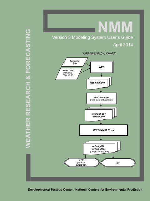
The WRF modeling system software is in the public domain and is freely available forcommunity use.The WRF-NMM System Program ComponentsFigure 1 shows a flowchart for the WRF-NMM System Version 3. As shown in thediagram, the WRF-NMM System consists of these major components:WRF Preprocessing System (WPS)WRF-NMM solverPostprocessor utilities and graphics tools including Unified Post Processor (UPP)and Read Interpolate Plot (RIP)Model Evaluation Tools (MET)WRF Preprocessing System (WPS)This program is used for real-data simulations. Its functions include:Defining the simulation domain;Interpolating terrestrial data (such as terrain, land-use, and soil types) to thesimulation domain;Degribbing and interpolating meteorological data from another model to thesimulation domain and the model coordinate.(For more details, see Chapter 3.)WRF-NMM SolverThe key features of the WRF-NMM are:Fully compressible, non-hydrostatic model with a hydrostatic option (Janjic,2003a).Hybrid (sigma-pressure) vertical coordinate.Arakawa E-grid.Forward-backward scheme for horizontally propagating fast waves, implicitscheme for vertically propagating sound waves, Adams-Bashforth Scheme forhorizontal advection, and Crank-Nicholson scheme for vertical advection. Thesame time step is used for all terms.Conservation of a number of first and second order quantities, including energyand enstrophy (Janjic 1984).Full physics options for land-surface, planetary boundary layer, atmospheric andsurface radiation, microphysics, and cumulus convection.One-way and two-way nesting with multiple nests and nest levels.(For more details and references, see Chapter 5.)WRF-NMM V3: User’s Guide 1-2

The WRF-NMM code contains an initialization program (real_nmm.exe; see Chapter 4)and a numerical integration program (wrf.exe; see Chapter 5).Unified Post Processor (UPP)This program can be used to post-process both WRF-ARW and WRF-NMM forecastsand was designed to:Interpolate the forecasts from the model’s native vertical coordinate to NWSstandard output levels.Destagger the forecasts from the staggered native grid to a regular non-staggeredgrid.Compute diagnostic output quantities.Output the results in NWS and WMO standard GRIB1.(For more details, see Chapter 7.)Read Interpolate Plot (RIP)This program can be used to plot both WRF-ARW and WRF-NMM forecasts. Somebasic features include:Uses a preprocessing program to read model output and convert this data intostandard RIP format data files.Makes horizontal plots, vertical cross sections and skew-T/log p soundings.Calculates and plots backward and forward trajectories.Makes a data set for use in the Vis5D software package.(For more details, see Chapter 7.)Model Evaluation Tools (MET)This verification package can be used to evaluate both WRF-ARW and WRF-NMMforecasts with the following techniques:Standard verification scores comparing gridded model data to point-basedobservationsStandard verification scores comparing gridded model data to griddedobservationsObject-based verification method comparing gridded model data to griddedobservationsMET is developed and supported by the Developmental Testbed Center and full detailscan be found on the MET User’s site at: http://www.dtcenter.org/met/users.WRF-NMM V3: User’s Guide 1-3

User's Guide for the NMM Core of theWeather Research and Forecast (WRF)Modeling System Version 3Chapter 2: Software InstallationTable of Contents Introduction Required Compilers and Scripting Languaugeso WRF System Software Requirementso WPS Software Requirements Required/Optional Libraries to Download UNIX Environment Settings Building the WRF System for the NMM Coreo Obtaining and Opening the WRF Packageo How to Configure WRFo How to Compile WRF for the NMM Core Building the WRF Preprocessing Systemo How to Install the WPSIntroductionThe WRF modeling system software installation is fairly straightforward on the portedplatforms listed below. The model-component portion of the package is mostly selfcontained.The WRF model does contain the source code to a Fortran interface to ESMFand the source to FFTPACK . Contained within the WRF system is the WRFDAcomponent, which has several external libraries that the user must install (for variousobservation types and linear algebra solvers). Similarly, the WPS package, separate fromthe WRF source code, has additional external libraries that must be built (in support ofGrib2 processing). The one external package that all of the systems require is thenetCDF library, which is one of the supported I/O API packages. The netCDF librariesand source code are available from the Unidata homepage at http://www.unidata.ucar.edu(select DOWNLOADS, registration required).The WRF model has been successfully ported to a number of Unix-based machines.WRF developers do not have access to all of them and must rely on outside users andvendors to supply the required configuration information for the compiler and loaderoptions. Below is a list of the supported combinations of hardware and software forWRF.WRF-NMM V3: User’s Guide 2-1

Vendor Hardware OS CompilerCray XC30 Intel Linux IntelCray XE AMD Linux IntelIBM Power Series AIX vendorIBM Intel Linux Intel / PGI / gfortranSGI IA64 / Opteron Linux IntelCOTS* IA32 LinuxCOTS IA64 / Opteron LinuxIntel / PGI /gfortran / g95 /PathScaleIntel / PGI /gfortran /PathScaleMac Power Series Darwin xlf / g95 / PGI / IntelMac Intel Darwingfortran / PGI / IntelNEC NEC Linux vendorFujitsu FX10 Intel Linux vendor* Commercial Off-The-Shelf systemsThe WRF model may be built to run on a single processor machine, a shared-memorymachine (that use the OpenMP API), a distributed memory machine (with the appropriateMPI libraries), or on a distributed cluster (utilizing both OpenMP and MPI). For WRF-NMM it is recommended at this time to compile either serial or utilizing distributedmemory. The WPS package also runs on the above listed systems.Required Compilers and Scripting LanguagesWRF System Software RequirementsThe WRF model is written in FORTRAN (what many refer to as FORTRAN 90). Thesoftware layer, RSL-LITE, which sits between WRF and the MPI interface, are written inC. Ancillary programs that perform file parsing and file construction, both of which arerequired for default building of the WRF modeling code, are written in C. Thus,FORTRAN 90 or 95 and C compilers are required. Additionally, the WRF buildmechanism uses several scripting languages: including perl (to handle various tasks suchas the code browser designed by Brian Fiedler), C-shell and Bourne shell. The traditionalUNIX text/file processing utilities are used: make, M4, sed, and awk. If OpenMPcompilation is desired, OpenMP libraries are required. The WRF I/O API also supportsWRF-NMM V3: User’s Guide 2-2

netCDF, PHD5 and GriB-1 formats, hence one of these libraries needs to be available onthe computer used to compile and run WRF.See Chapter 6: WRF Software (Required Software) for a more detailed listing of thenecessary pieces for the WRF build.WPS Software RequirementsThe WRF Preprocessing System (WPS) requires the same Fortran and C compilers usedto build the WRF model. WPS makes direct calls to the MPI libraries for distributedmemory message passing. In addition to the netCDF library, the WRF I/O API librarieswhich are included with the WRF model tar file are also required. In order to run theWRF Domain Wizard, which allows you to easily create simulation domains, Java 1.5 orlater is recommended.Required/Optional Libraries to DownloadThe netCDF package is required and can be downloaded from Unidata:http://www.unidata.ucar.edu (select DOWNLOADS).The netCDF libraries should be installed either in the directory included in the user’s pathto netCDF libraries or in /usr/local and its include/ directory is defined by theenvironmental variable NETCDF. For example:setenv NETCDF /path-to-netcdf-libraryTo execute netCDF commands, such as ncdump and ncgen, /path-to-netcdf/bin may alsoneed to be added to the user’s path.Hint: When compiling WRF codes on a Linux system using the PGI (Intel, g95, gfortran)compiler, make sure the netCDF library has been installed using the same PGI (Intel,g95, gfortran) compiler.Hint: On NCAR’s IBM computer, the netCDF library is installed for both 32-bit and 64-bit memory usage. The default would be the 32-bit version. If you would like to use the64-bit version, set the following environment variable before you start compilation:setenv OBJECT_MODE 64If distributed memory jobs will be run, a version of MPI is required prior to building theWRF-NMM. A version of mpich for LINUX-PCs can be downloaded from:http://www-unix.mcs.anl.gov/mpi/mpichThe user may want their system administrator to install the code. To determine whetherMPI is available on your computer system, try:which mpif90which mpiccWRF-NMM V3: User’s Guide 2-3

which mpirunIf all of these executables are defined, MPI is probably already available. The MPI lib/,include/, and bin/ need to be included in the user’s path.Three libraries are required by the WPS ungrib program for GRIB Edition 2 compressionsupport. Users are encouraged to engage their system administrators support for theinstallation of these packages so that traditional library paths and include paths aremaintained. Paths to user-installed compression libraries are handled in theconfigure.wps file by the COMPRESSION_LIBS and COMPRESSION_INC variables.As an alternative to manually editing the COMPRESSION_LIBS andCOMPRESSION_INC variables in the configure.wps file, users may set theenvironment variables JASPERLIB and JASPERINC to the directories holding theJasPer library and include files before configuring the WPS; for example, if the JasPerlibraries were installed in /usr/local/jasper-1.900.1, one might use the followingcommands (in csh or tcsh):setenv JASPERLIB /usr/local/jasper-1.900.1/libsetenv JASPERINC /usr/local/jasper-1.900.1/includeIf the zlib and PNG libraries are not in a standard path that will be checked automaticallyby the compiler, the paths to these libraries can be added on to the JasPer environmentvariables; for example, if the PNG libraries were installed in /usr/local/libpng-1.2.29 andthe zlib libraries were installed in /usr/local/zlib-1.2.3, one might usesetenv JASPERLIB “${JASPERLIB} -L/usr/local/libpng-1.2.29/lib-L/usr/local/zlib-1.2.3/lib”setenv JASPERINC “${JASPERINC} -I/usr/local/libpng-1.2.29/include-I/usr/local/zlib-1.2.3/include”after having previously set JASPERLIB and JASPERINC.1. JasPer (an implementation of the JPEG2000 standard for "lossy" compression)http://www.ece.uvic.ca/~mdadams/jasper/Go down to “JasPer software”, one of the "click here" parts is the source../configuremakemake installNote: The GRIB2 libraries expect to find include files in jasper/jasper.h, so itmay be necessary to manually create a jasper subdirectory in the includedirectory created by the JasPer installation, and manually link header files there.2. zlib (another compression library, which is used by the PNG library)http://www.zlib.net/Go to "The current release is publicly available here" section and download.WRF-NMM V3: User’s Guide 2-4

./configuremakemake install3. PNG (compression library for "lossless" compression)http://www.libpng.org/pub/png/libpng.htmlScroll down to "Source code" and choose a mirror site../configuremake checkmake installTo get around portability issues, the NCEP GRIB libraries, w3 and g2, have beenincluded in the WPS distribution. The original versions of these libraries are available fordownload from NCEP at http://www.nco.ncep.noaa.gov/pmb/codes/GRIB2/. The specifictar files to download are g2lib and w3lib. Because the ungrib program requires modulesfrom these files, they are not suitable for usage with a traditional library option during thelink stage of the build.UNIX Environment SettingsPath names for the compilers and libraries listed above should be defined in the shellconfiguration files (such as .cshrc or .login). For example:set path = ( /usr/pgi/bin /usr/pgi/lib /usr/local/ncarg/bin \/usr/local/mpich-pgi /usr/local/mpich-pgi/bin \/usr/local/netcdf-pgi/bin /usr/local/netcdf-pgi/include)setenv PGI /usr/pgisetenv NETCDF /usr/local/netcdf-pgisetenv NCARG_ROOT /usr/local/ncargsetenv LM_LICENSE_FILE $PGI/license.datsetenv LD_LIBRARY_PATH /usr/lib:/usr/local/lib:/usr/pgi/linux86/lib:/usr/local/netcdf-pgi/libIn addition, there are a few WRF-related environmental settings. To build the WRF-NMM core, the environment setting WRF_NMM_CORE is required. If nesting will beused, the WRF_NMM_NEST environment setting needs to be specified (see below). Asingle domain can still be specified even if WRF_NMM_NEST is set to 1. If the WRF-NMM will be built for the HWRF configuration, the HWRF environment setting alsoneeds to be set (see below). The rest of these settings are not required, but the user maywant to try some of these settings if difficulties are encountered during the build process.In C-shell syntax:setenv WRF_NMM_CORE 1 (explicitly turns on WRF-NMM core to build)setenv WRF_NMM_NEST 1 (nesting is desired using the WRF-NMM core)WRF-NMM V3: User’s Guide 2-5

setenv HWRF 1 (explicitly specifies that WRF-NMM will be built for theHWRF configuration; set along with previous two environment settings)unset limits (especially if you are on a small system)setenv MP_STACK_SIZE 64000000 (OpenMP blows through the stack size, setit large)setenv MPICH_F90 f90 (or whatever your FORTRAN compiler may be called.WRF needs the bin, lib, and include directories)setenv OMP_NUM_THREADS n (where n is the number of processors to use. Insystems with OpenMP installed, this is how the number of threads is specified.)Building the WRF System for the NMM CoreObtaining and Opening the WRF PackageThe WRF-NMM source code tar file may be downloaded from:http://www.dtcenter.org/wrf-nmm/users/downloads/Note: Always obtain the latest version of the code if you are not trying to continue a preexistingproject. WRFV3 is just used as an example here.Once the tar file is obtained, gunzip and untar the file.tar –zxvf WRFV3.TAR.gzThe end product will be a WRFV3/ directory that contains:MakefileREADMEREADME.DAREADME.io_configREADME.NMMREADME.rsl_outputREADME.SSIBREADME_test_casesREADME.windturbineRegistry/arch/chem/cleancompileconfiguredyn_emdyn_exp/dyn_nmm/external/frame/Top-level makefileGeneral information about WRF codeGeneral information about WRFDA codeIO stream informationNMM specific informationExplanation of the another rsl.* output optionInformation about coupling WRF-ARW with SSiBDirections for running test cases and a listing of casesDescribes wind turbine drag parameterization schemesDirectory for WRF Registry fileDirectory where compile options are gatheredDirectory for WRF-ChemScript to clean created files and executablesScript for compiling WRF codeScript to configure the configure.wrf file for compileDirectory for WRF-ARW dynamic modulesDirectory for a 'toy' dynamic coreDirectory for WRF-NMM dynamic modulesDirectory that contains external packages, such as thosefor IO, time keeping, ocean coupling interface and MPIDirectory that contains modules for WRF frameworkWRF-NMM V3: User’s Guide 2-6

inc/main/phys/run/share/test/tools/var/Directory that contains include filesDirectory for main routines, such as wrf.F, and allexecutablesDirectory for all physics modulesDirectory where one may run WRFDirectory that contains mostly modules for WRFmediation layer and WRF I/ODirectory containing sub-directories where one may runspecific configurations of WRF - Only nmm_real isrelevant to WRF-NMMDirectory that contains toolsDirectory for WRF-VarHow to Configure the WRFThe WRF code has a fairly sophisticated build mechanism. The package tries todetermine the architecture on which the code is being built, and then presents the userwith options to allow the user to select the preferred build method. For example, on aLinux machine, the build mechanism determines whether the machine is 32- or 64-bit,and then prompts the user for the desired usage of processors (such as serial, sharedmemory, or distributed memory).A helpful guide to building WRF using PGI compilers on a 32-bit or 64-bit LINUXsystem can be found at:http://www.pgroup.com/resources/tips.htm#WRF.To configure WRF, go to the WRF (top) directory (cd WRF) and type:./configureYou will be given a list of choices for your computer. These choices range fromcompiling for a single processor job (serial), to using OpenMP shared-memory (SM) ordistributed-memory (DM) parallelization options for multiple processors.Choices for a LINUX operating systems include:1. Linux x86_64, PGI compiler with gcc (serial)2. Linux x86_64, PGI compiler with gcc (smpar)3. Linux x86_64, PGI compiler with gcc (dmpar)4. Linux x86_64, PGI compiler with gcc (dm+sm)5. Linux x86_64, PGI compiler with pgcc, SGI MPT (serial)6. Linux x86_64, PGI compiler with pgcc, SGI MPT (smpar)7. Linux x86_64, PGI compiler with pgcc, SGI MPT (dmpar)8. Linux x86_64, PGI compiler with pgcc, SGI MPT (dm+sm)9. Linux x86_64, PGI accelerator compiler with gcc (serial)10. Linux x86_64, PGI accelerator compiler with gcc (smpar)11. Linux x86_64, PGI accelerator compiler with gcc (dmpar)12. Linux x86_64, PGI accelerator compiler with gcc (dm+sm)13. Linux x86_64 i486 i586 i686, ifort compiler with icc (serial)WRF-NMM V3: User’s Guide 2-7

14. Linux x86_64 i486 i586 i686, ifort compiler with icc (smpar)15. Linux x86_64 i486 i586 i686, ifort compiler with icc (dmpar)16. Linux x86_64 i486 i586 i686, ifort compiler with icc (dm+sm)17. Linux x86_64 i486 i586 i686, ifort compiler with icc, SGI MPT (serial)18. Linux x86_64 i486 i586 i686, ifort compiler with icc, SGI MPT (smpar)19. Linux x86_64 i486 i586 i686, ifort compiler with icc, SGI MPT (dmpar)20. Linux x86_64 i486 i586 i686, ifort compiler with icc, SGI MPT (dm+sm)…For WRF-NMM V3 on LINUX operating systems, option 3 is recommended.Note: For WRF-NMM it is recommended at this time to compile either serial or utilizingdistributed memory (DM).Once an option is selected, a choice of what type of nesting is desired (no nesting (0),basic (1), pre-set moves (2), or vortex following (3)) will be given. For WRF-NMM,only no nesting or ‘basic’ nesting is available at this time, unless the environment settingHWRF is set, then (3) will be automatically selected, which will enable the HWRF vortexfollowing moving nest capability.Check the configure.wrf file created and edit for compile options/paths, if necessary.Hint: It is helpful to start with something simple, such as the serial build. If it issuccessful, move on to build smpar or dmpar code. Remember to type ‘clean –a’ betweeneach build.Hint: If you anticipate generating a netCDF file that is larger than 2Gb (whether it is asingle- or multi-time period data [e.g. model history]) file), you may set the followingenvironment variable to activate the large-file support option from netCDF (in c-shell):setenv WRFIO_NCD_LARGE_FILE_SUPPORT 1Hint: If you would like to use parallel netCDF (p-netCDF) developed by ArgonneNational Lab (http://trac.mcs.anl.gov/projects/parallel-netcdf), you will need to install p-netCDF separately, and use the environment variable PNETCDF to set the path:setenv PNETCDF path-to-pnetcdf-libraryHint: Since V3.5, compilation may take a bit longer due to the addition of the CLM4module. If you do not intend to use the CLM4 land-surface model option, you canmodify your configure.wrf file by removing -DWRF_USE_CLM fromARCH_LOCAL.How to Compile WRF for the NMM coreTo compile WRF for the NMM dynamic core, the following environment variable mustbe set:setenv WRF_NMM_CORE 1WRF-NMM V3: User’s Guide 2-8

If compiling for nested runs, also set:setenv WRF_NMM_NEST 1Note: A single domain can be specified even if WRF_NMM_NEST is set to 1.If compiling for HWRF, also set:setenv HWRF 1Once these environment variables are set, enter the following command:./compile nmm_realNote that entering:./compile -hor./compileproduces a listing of all of the available compile options (only nmm_real is relevant tothe WRF-NMM core).To remove all object files (except those in external/) and executables, type:cleanTo remove all built files in ALL directories, as well as the configure.wrf, type:clean –aThis action is recommended if a mistake is made during the installation process, or if theRegistry.NMM* or configure.wrf files have been edited.When the compilation is successful, two executables are created in main/:real_nmm.exe: WRF-NMM initializationwrf.exe: WRF-NMM model integrationThese executables are linked to run/ and test/nmm_real/. The test/nmm_real and rundirectories are working directories that can be used for running the model.Beginning with V3.5, the compression function in netCDF4 is supported. This option willtypically reduce the file size by more than 50%. It will require netCDF4 to be installedwith the option --enable-netcdf-4. Before compiling WRF, you will need to setthe environment variable NETCDF4. In a C-shell environment, type;WRF-NMM V3: User’s Guide 2-9

compile_wps.outconfigureconfigure.wpsgeogrid/geogrid.exe -> geogrid/src/geogrid.exelink_grib.cshmetgrid/namelist.wps.firenamelist.wps.globalnamelist.wps.nmmREADMEungrib/ungrib.exe -> ungrib/src/ungrib.exeutil/More details on the functions of the WPS and how to run it can be found in Chapter 3.WRF-NMM V3: User’s Guide 2-11

User's Guide for the NMM Core of theWeather Research and Forecast (WRF)Modeling System Version 3Chapter 3: WRF Preprocessing System (WPS)Table of ContentsIntroductionFunction of Each WPS ProgramRunning the WPSCreating Nested Domains with the WPSSelecting Between USGS and MODIS-based Land Use DataStatic Data for the Gravity Wave Drag SchemeUsing Multiple Meteorological Data SourcesAlternative Initialization of Lake SSTsParallelism in the WPSChecking WPS OutputWPS Utility ProgramsWRF Domain WizardWriting Meteorological Data to the Intermediate FormatCreating and Editing VtablesWriting Static Data to the Geogrid Binary FormatDescription of Namelist VariablesDescription of GEOGRID.TBL OptionsDescription of index OptionsDescription of METGRID.TBL OptionsAvailable Interpolation Options in Geogrid and MetgridLand Use and Soil Categories in the Static DataWPS Output FieldsIntroductionThe WRF Preprocessing System (WPS) is a set of three programs whose collective role isto prepare input to the real program for real-data simulations. Each of the programsperforms one stage of the preparation: geogrid defines model domains and interpolatesstatic geographical data to the grids; ungrib extracts meteorological fields from GRIBformattedfiles; and metgrid horizontally interpolates the meteorological fields extractedWRF-NMM V3: User’s Guide 3-1

y ungrib to the model grids defined by geogrid. The work of vertically interpolatingmeteorological fields to WRF eta levels is performed within the real program.External DataSourcesStaticGeographicalDataWRF Preprocessing Systemgeogridnamelist.wps(static file(s) for nested runs)metgridreal_nmmGridded Data:NAM, GFS,RUC,AGRMET,etc.ungribwrfThe data flow between the programs of the WPS is shown in the figure above. Each ofthe WPS programs reads parameters from a common namelist file, as shown in the figure.This namelist file has separate namelist records for each of the programs and a sharednamelist record, which defines parameters that are used by more than one WPS program.Not shown in the figure are additional table files that are used by individual programs.These tables provide additional control over the programs’ operation, though theygenerally do not need to be changed by the user. The GEOGRID.TBL, METGRID.TBL,and Vtable files are explained later in this document, though for now, the user need notbe concerned with them.The build mechanism for the WPS, which is very similar to the build mechanism used bythe WRF model, provides options for compiling the WPS on a variety of platforms.When MPICH libraries and suitable compilers are available, the metgrid and geogridprograms may be compiled for distributed memory execution, which allows large modeldomains to be processed in less time. The work performed by the ungrib program is notamenable to parallelization, so ungrib may only be run on a single processor.Function of Each WPS ProgramThe WPS consists of three independent programs: geogrid, ungrib, and metgrid. Alsoincluded in the WPS are several utility programs, which are described in the section onutility programs. A brief description of each of the three main programs is given below,with further details presented in subsequent sections.Program geogridWRF-NMM V3: User’s Guide 3-2

The purpose of geogrid is to define the simulation domains, and interpolate variousterrestrial data sets to the model grids. The simulation domains are defined usinginformation specified by the user in the “geogrid” namelist record of the WPS namelistfile, namelist.wps. In addition to computing the latitude, longitude, and map scale factorsat every grid point, geogrid will interpolate soil categories, land use category, terrainheight, annual mean deep soil temperature, monthly vegetation fraction, monthly albedo,maximum snow albedo, and slope category to the model grids by default. Global data setsfor each of these fields are provided through the WRF download page, and, because thesedata are time-invariant, they only need to be downloaded once. Several of the data setsare available in only one resolution, but others are made available in resolutions of 30",2', 5', and 10'; here, " denotes arc seconds and ' denotes arc minutes. The user need notdownload all available resolutions for a data set, although the interpolated fields willgenerally be more representative if a resolution of data near to that of the simulationdomain is used. However, users who expect to work with domains having grid spacingsthat cover a large range may wish to eventually download all available resolutions of thestatic terrestrial data.Besides interpolating the default terrestrial fields, the geogrid program is general enoughto be able to interpolate most continuous and categorical fields to the simulation domains.New or additional data sets may be interpolated to the simulation domain through the useof the table file, GEOGRID.TBL. The GEOGRID.TBL file defines each of the fields thatwill be produced by geogrid; it describes the interpolation methods to be used for a field,as well as the location on the file system where the data set for that field is located.Output from geogrid is written in the WRF I/O API format, and thus, by selecting theNetCDF I/O format, geogrid can be made to write its output in NetCDF for easyvisualization using external software packages, including ncview, NCL, and RIP4.Program ungribThe ungrib program reads GRIB files, "degribs" the data, and writes the data in a simpleformat, called the intermediate format (see the section on writing data to the intermediateformat for details of the format). The GRIB files contain time-varying meteorologicalfields and are typically from another regional or global model, such as NCEP's NAM orGFS models. The ungrib program can read GRIB Edition 1 and, if compiled with a"GRIB2" option, GRIB Edition 2 files.GRIB files typically contain more fields than are needed to initialize WRF. Both versionsof the GRIB format use various codes to identify the variables and levels in the GRIBfile. Ungrib uses tables of these codes – called Vtables, for "variable tables" – to definewhich fields to extract from the GRIB file and write to the intermediate format. Detailsabout the codes can be found in the WMO GRIB documentation and in documentationfrom the originating center. Vtables for common GRIB model output files are providedwith the ungrib software.WRF-NMM V3: User’s Guide 3-3

Vtables are provided for NAM 104 and 212 grids, the NAM AWIP format, GFS, theNCEP/NCAR Reanalysis archived at NCAR, RUC (pressure level data and hybridcoordinate data), AFWA's AGRMET land surface model output, ECMWF, and other datasets. Users can create their own Vtable for other model output using any of the Vtables asa template; further details on the meaning of fields in a Vtable are provided in the sectionon creating and editing Vtables.Ungrib can write intermediate data files in any one of three user-selectable formats: WPS– a new format containing additional information useful for the downstream programs; SI– the previous intermediate format of the WRF system; and MM5 format, which isincluded here so that ungrib can be used to provide GRIB2 input to the MM5 modelingsystem. Any of these formats may be used by WPS to initialize WRF, although the WPSformat is recommended.Program metgridThe metgrid program horizontally interpolates the intermediate-format meteorologicaldata that are extracted by the ungrib program onto the simulation domains defined by thegeogrid program. The interpolated metgrid output can then be ingested by the WRF realprogram. The range of dates that will be interpolated by metgrid are defined in the“share” namelist record of the WPS namelist file, and date ranges must be specifiedindividually in the namelist for each simulation domain. Since the work of the metgridprogram, like that of the ungrib program, is time-dependent, metgrid is run every time anew simulation is initialized.Control over how each meteorological field is interpolated is provided by theMETGRID.TBL file. The METGRID.TBL file provides one section for each field, andwithin a section, it is possible to specify options such as the interpolation methods to beused for the field, the field that acts as the mask for masked interpolations, and the gridstaggering (e.g., U, V in ARW; H, V in NMM) to which a field is interpolated.Output from metgrid is written in the WRF I/O API format, and thus, by selecting theNetCDF I/O format, metgrid can be made to write its output in NetCDF for easyvisualization using external software packages, including the new version of RIP4.Running the WPSNote: For software requirements and how to compile the WRF Preprocessing Systempackage, see Chapter 2.There are essentially three main steps to running the WRF Preprocessing System:1. Define a model coarse domain and any nested domains with geogrid.2. Extract meteorological fields from GRIB data sets for the simulation period withungrib.3. Horizontally interpolate meteorological fields to the model domains with metgrid.WRF-NMM V3: User’s Guide 3-4

When multiple simulations are to be run for the same model domains, it is only necessaryto perform the first step once; thereafter, only time-varying data need to be processed foreach simulation using steps two and three. Similarly, if several model domains are beingrun for the same time period using the same meteorological data source, it is notnecessary to run ungrib separately for each simulation. Below, the details of each of thethree steps are explained.Step 1: Define model domains with geogridIn the root of the WPS directory structure, symbolic links to the programs geogrid.exe,ungrib.exe, and metgrid.exe should exist if the WPS software was successfully installed.In addition to these three links, a namelist.wps file should exist. Thus, a listing in theWPS root directory should look something like:> lsdrwxr-xr-x 2 4096 arch-rwxr-xr-x 1 1672 clean-rwxr-xr-x 1 3510 compile-rw-r--r-- 1 85973 compile.output-rwxr-xr-x 1 4257 configure-rw-r--r-- 1 2486 configure.wpsdrwxr-xr-x 4 4096 geogridlrwxrwxrwx 1 23 geogrid.exe -> geogrid/src/geogrid.exe-rwxr-xr-x 1 1328 link_grib.cshdrwxr-xr-x 3 4096 metgridlrwxrwxrwx 1 23 metgrid.exe -> metgrid/src/metgrid.exe-rw-r--r-- 1 1101 namelist.wps-rw-r--r-- 1 1987 namelist.wps.all_options-rw-r--r-- 1 1075 namelist.wps.global-rw-r--r-- 1 652 namelist.wps.nmm-rw-r--r-- 1 4786 READMEdrwxr-xr-x 4 4096 ungriblrwxrwxrwx 1 21 ungrib.exe -> ungrib/src/ungrib.exedrwxr-xr-x 3 4096 utilThe model coarse domain and any nested domains are defined in the “geogrid” namelistrecord of the namelist.wps file, and, additionally, parameters in the “share” namelistrecord need to be set. An example of these two namelist records is given below, and theuser is referred to the description of namelist variables for more information on thepurpose and possible values of each variable.&sharewrf_core = 'NMM',max_dom = 2,start_date = '2008-03-24_12:00:00','2008-03-24_12:00:00',end_date = '2008-03-24_18:00:00','2008-03-24_12:00:00',interval_seconds = 21600,io_form_geogrid = 2/&geogridparent_id = 1, 1,parent_grid_ratio = 1, 3,i_parent_start = 1, 31,j_parent_start = 1, 17,e_we = 74, 112,WRF-NMM V3: User’s Guide 3-5

e_sn = 61, 97,geog_data_res = '10m','2m',dx = 0.289153,dy = 0.287764,map_proj = 'rotated_ll',ref_lat = 34.83,ref_lon = -81.03,geog_data_path = '/mmm/users/wrfhelp/WPS_GEOG/'/To summarize a set of typical changes to the “share” namelist record relevant to geogrid,the WRF dynamical core must first be selected with wrf_core. If WPS is being run foran ARW simulation, wrf_core should be set to 'ARW', and if running for an NMMsimulation, it should be set to 'NMM'. After selecting the dynamical core, the total numberof domains (in the case of ARW) or nesting levels (in the case of NMM) must be chosenwith max_dom. Since geogrid produces only time-independent data, the start_date,end_date, and interval_seconds variables are ignored by geogrid. Optionally, alocation (if not the default, which is the current working directory) where domain filesshould be written to may be indicated with the opt_output_from_geogrid_pathvariable, and the format of these domain files may be changed with io_form_geogrid.In the “geogrid” namelist record, the projection of the simulation domain is defined, asare the size and location of all model grids. The map projection to be used for the modeldomains is specified with the map_proj variable and must be set to rotated_ll forWRF-NMM.Besides setting variables related to the projection, location, and coverage of modeldomains, the path to the static geographical data sets must be correctly specified with thegeog_data_path variable. Also, the user may select which resolution of static datageogrid will interpolate from using the geog_data_res variable, whose value shouldmatch one of the resolutions of data in the GEOGRID.TBL. If the full set of static dataare downloaded from the WRF download page, possible resolutions include '30s', '2m','5m', and '10m', corresponding to 30-arc-second data, 2-, 5-, and 10-arc-minute data.Depending on the value of the wrf_core namelist variable, the appropriateGEOGRID.TBL file must be used with geogrid, since the grid staggerings that WPSinterpolates to differ between dynamical cores. For the ARW, the GEOGRID.TBL.ARWfile should be used, and for the NMM, the GEOGRID.TBL.NMM file should be used.Selection of the appropriate GEOGRID.TBL is accomplished by linking the correct fileto GEOGRID.TBL in the geogrid directory (or in the directory specified byopt_geogrid_tbl_path, if this variable is set in the namelist).> ls geogrid/GEOGRID.TBLlrwxrwxrwx 115 GEOGRID.TBL -> GEOGRID.TBL.NMMFor more details on the meaning and possible values for each variable, the user is referredto a description of the namelist variables.WRF-NMM V3: User’s Guide 3-6

Having suitably defined the simulation coarse domain and nested domains in thenamelist.wps file, the geogrid.exe executable may be run to produce domain files. In thecase of ARW domains, the domain files are named geo_em.d0N.nc, where N is thenumber of the nest defined in each file. When run for NMM domains, geogrid producesthe file geo_nmm.d01.nc for the coarse domain, and geo_nmm_nest.l0N.nc files foreach nesting level N. Also, note that the file suffix will vary depending on theio_form_geogrid that is selected. To run geogrid, issue the following command:> ./geogrid.exeWhen geogrid.exe has finished running, the message!!!!!!!!!!!!!!!!!!!!!!!!!!!!!!!!!!!!!!!!!!!!!! Successful completion of geogrid. !!!!!!!!!!!!!!!!!!!!!!!!!!!!!!!!!!!!!!!!!!!!!!should be printed, and a listing of the WPS root directory (or the directory specified byopt_output_from_geogrid_path, if this variable was set) should show the domain files.If not, the geogrid.log file may be consulted in an attempt to determine the possible causeof failure. For more information on checking the output of geogrid, the user is referred tothe section on checking WPS output.> lsdrwxr-xr-x 2 4096 arch-rwxr-xr-x 1 1672 clean-rwxr-xr-x 1 3510 compile-rw-r--r-- 1 85973 compile.output-rwxr-xr-x 1 4257 configure-rw-r--r-- 1 2486 configure.wps-rw-r--r-- 1 1957004 geo_nmm.d01.nc-rw-r--r-- 1 4745324 geo_nmm.d02.ncdrwxr-xr-x 4 4096 geogridlrwxrwxrwx 1 23 geogrid.exe -> geogrid/src/geogrid.exe-rw-r--r-- 1 11169 geogrid.log-rwxr-xr-x 1 1328 link_grib.cshdrwxr-xr-x 3 4096 metgridlrwxrwxrwx 1 23 metgrid.exe -> metgrid/src/metgrid.exe-rw-r--r-- 1 1094 namelist.wps-rw-r--r-- 1 1987 namelist.wps.all_options-rw-r--r-- 1 1075 namelist.wps.global-rw-r--r-- 1 652 namelist.wps.nmm-rw-r--r-- 1 4786 READMEdrwxr-xr-x 4 4096 ungriblrwxrwxrwx 1 21 ungrib.exe -> ungrib/src/ungrib.exedrwxr-xr-x 3 4096 utilStep 2: Extracting meteorological fields from GRIB files with ungribHaving already downloaded meteorological data in GRIB format, the first step inextracting fields to the intermediate format involves editing the “share” and “ungrib”namelist records of the namelist.wps file – the same file that was edited to define thesimulation domains. An example of the two namelist records is given below.WRF-NMM V3: User’s Guide 3-7

&sharewrf_core = 'NMM',max_dom = 2,start_date = '2008-03-24_12:00:00','2008-03-24_12:00:00',end_date = '2008-03-24_18:00:00','2008-03-24_12:00:00',interval_seconds = 21600,io_form_geogrid = 2/&ungribout_format = 'WPS',prefix = 'FILE'/In the “share” namelist record, the variables that are of relevance to ungrib are thestarting and ending times of the coarse domain (start_date and end_date; alternatively,start_year, start_month, start_day, start_hour, end_year, end_month, end_day,and end_hour) and the interval between meteorological data files (interval_seconds).In the “ungrib” namelist record, the variable out_format is used to select the format ofthe intermediate data to be written by ungrib; the metgrid program can read any of theformats supported by ungrib, and thus, any of 'WPS', 'SI', and 'MM5' may be specifiedfor out_format, although 'WPS' is recommended. Also in the "ungrib" namelist, the usermay specify a path and prefix for the intermediate files with the prefix variable. Forexample, if prefix were set to 'ARGRMET', then the intermediate files created by ungribwould be named according to AGRMET:YYYY-MM-DD_HH, where YYYY-MM-DD_HHis the valid time of the data in the file.After suitably modifying the namelist.wps file, a Vtable must be supplied, and the GRIBfiles must be linked (or copied) to the filenames that are expected by ungrib. The WPS issupplied with Vtable files for many sources of meteorological data, and the appropriateVtable may simply be symbolically linked to the file Vtable, which is the Vtable nameexpected by ungrib. For example, if the GRIB data are from the GFS model, this could beaccomplished with> ln -s ungrib/Variable_Tables/Vtable.GFS VtableThe ungrib program will try to read GRIB files named GRIBFILE.AAA,GRIBFILE.AAB, …, GRIBFILE.ZZZ. In order to simplify the work of linking the GRIBfiles to these filenames, a shell script, link_grib.csh, is provided. The link_grib.csh scripttakes as a command-line argument a list of the GRIB files to be linked. For example, ifthe GRIB data were downloaded to the directory /data/gfs, the files could be linked withlink_grib.csh as follows:> ls /data/gfs-rw-r--r-- 1 42728372 gfs_080324_12_00-rw-r--r-- 1 48218303 gfs_080324_12_06> ./link_grib.csh /data/gfs/gfs*After linking the GRIB files and Vtable, a listing of the WPS directory should looksomething like the following:WRF-NMM V3: User’s Guide 3-8

lsdrwxr-xr-x 2 4096 arch-rwxr-xr-x 1 1672 clean-rwxr-xr-x 1 3510 compile-rw-r--r-- 1 85973 compile.output-rwxr-xr-x 1 4257 configure-rw-r--r-- 1 2486 configure.wps-rw-r--r-- 1 1957004 geo_nmm.d01.nc-rw-r--r-- 1 4745324 geo_nmm.d02.ncdrwxr-xr-x 4 4096 geogridlrwxrwxrwx 1 23 geogrid.exe -> geogrid/src/geogrid.exe-rw-r--r-- 1 11169 geogrid.loglrwxrwxrwx 1 38 GRIBFILE.AAA -> /data/gfs/gfs_080324_12_00lrwxrwxrwx 1 38 GRIBFILE.AAB -> /data/gfs/gfs_080324_12_06-rwxr-xr-x 1 1328 link_grib.cshdrwxr-xr-x 3 4096 metgridlrwxrwxrwx 1 23 metgrid.exe -> metgrid/src/metgrid.exe-rw-r--r-- 1 1094 namelist.wps-rw-r--r-- 1 1987 namelist.wps.all_options-rw-r--r-- 1 1075 namelist.wps.global-rw-r--r-- 1 652 namelist.wps.nmm-rw-r--r-- 1 4786 READMEdrwxr-xr-x 4 4096 ungriblrwxrwxrwx 1 21 ungrib.exe -> ungrib/src/ungrib.exedrwxr-xr-x 3 4096 utillrwxrwxrwx 1 33 Vtable -> ungrib/Variable_Tables/Vtable.GFSAfter editing the namelist.wps file and linking the appropriate Vtable and GRIB files, theungrib.exe executable may be run to produce files of meteorological data in theintermediate format. Ungrib may be run by simply typing the following:> ./ungrib.exe >& ungrib.outputSince the ungrib program may produce a significant volume of output, it is recommendedthat ungrib output be redirected to a file, as in the command above. If ungrib.exe runssuccessfully, the message!!!!!!!!!!!!!!!!!!!!!!!!!!!!!!!!!!!!!!!!!!!!!! Successful completion of ungrib. !!!!!!!!!!!!!!!!!!!!!!!!!!!!!!!!!!!!!!!!!!!!!!will be written to the end of the ungrib.output file, and the intermediate files shouldappear in the current working directory. The intermediate files written by ungrib willhave names of the form FILE:YYYY-MM-DD_HH (unless, of course, the prefix variablewas set to a prefix other than 'FILE').> lsdrwxr-xr-x 2 4096 arch-rwxr-xr-x 1 1672 clean-rwxr-xr-x 1 3510 compile-rw-r--r-- 1 85973 compile.output-rwxr-xr-x 1 4257 configure-rw-r--r-- 1 2486 configure.wps-rw-r--r-- 1 154946888 FILE:2008-03-24_12-rw-r--r-- 1 154946888 FILE:2008-03-24_18-rw-r--r-- 1 1957004 geo_nmm.d01.nc-rw-r--r-- 1 4745324 geo_nmm.d02.ncdrwxr-xr-x 4 4096 geogridWRF-NMM V3: User’s Guide 3-9

lrwxrwxrwx 123 geogrid.exe -> geogrid/src/geogrid.exe-rw-r--r-- 1 11169 geogrid.loglrwxrwxrwx 138 GRIBFILE.AAA -> /data/gfs/gfs_080324_12_00lrwxrwxrwx 138 GRIBFILE.AAB -> /data/gfs/gfs_080324_12_06-rwxr-xr-x 1 1328 link_grib.cshdrwxr-xr-x 3 4096 metgridlrwxrwxrwx 123 metgrid.exe -> metgrid/src/metgrid.exe-rw-r--r-- 1 1094 namelist.wps-rw-r--r-- 1 1987 namelist.wps.all_options-rw-r--r-- 1 1075 namelist.wps.global-rw-r--r-- 1652 namelist.wps.nmm-rw-r--r-- 1 4786 READMEdrwxr-xr-x 4 4096 ungriblrwxrwxrwx 121 ungrib.exe -> ungrib/src/ungrib.exe-rw-r--r-- 1 1418 ungrib.log-rw-r--r-- 1 27787 ungrib.outputdrwxr-xr-x 3 4096 utillrwxrwxrwx 1 33 Vtable ->ungrib/Variable_Tables/Vtable.GFSStep 3: Horizontally interpolating meteorological data with metgridIn the final step of running the WPS, meteorological data extracted by ungrib arehorizontally interpolated to the simulation grids defined by geogrid. In order to runmetgrid, the namelist.wps file must be edited. In particular, the “share” and “metgrid”namelist records are of relevance to the metgrid program. Examples of these records areshown below.&sharewrf_core = 'NMM',max_dom = 2,start_date = '2008-03-24_12:00:00','2008-03-24_12:00:00',end_date = '2008-03-24_18:00:00','2008-03-24_12:00:00',interval_seconds = 21600,io_form_geogrid = 2/&metgridfg_name= 'FILE',io_form_metgrid = 2,/By this point, there is generally no need to change any of the variables in the “share”namelist record, since those variables should have been suitably set in previous steps. Ifthe "share" namelist was not edited while running geogrid and ungrib, however, the WRFdynamical core, number of domains, starting and ending times, interval betweenmeteorological data, and path to the static domain files must be set in the “share”namelist record, as described in the steps to run geogrid and ungrib.In the “metgrid” namelist record, the path and prefix of the intermediate meteorologicaldata files must be given with fg_name, the full path and file names of any intermediatefiles containing constant fields may be specified with the constants_name variable, andthe output format for the horizontally interpolated files may be specified with theio_form_metgrid variable. Other variables in the “metgrid” namelist record, namely,WRF-NMM V3: User’s Guide 3-10

opt_output_from_metgrid_path and opt_metgrid_tbl_path, allow the user tospecify where interpolated data files should be written by metgrid and where theMETGRID.TBL file may be found.As with geogrid and the GEOGRID.TBL file, a METGRID.TBL file appropriate for theWRF core must be linked in the metgrid directory (or in the directory specified byopt_metgrid_tbl_path, if this variable is set).> ls metgrid/METGRID.TBLlrwxrwxrwx 115 METGRID.TBL -> METGRID.TBL.NMMAfter suitably editing the namelist.wps file and verifying that the correct METGRID.TBLwill be used, metgrid may be run by issuing the command> ./metgrid.exeIf metgrid successfully ran, the message!!!!!!!!!!!!!!!!!!!!!!!!!!!!!!!!!!!!!!!!!!!!!! Successful completion of metgrid. !!!!!!!!!!!!!!!!!!!!!!!!!!!!!!!!!!!!!!!!!!!!!!will be printed. After successfully running, metgrid output files should appear in the WPSroot directory (or in the directory specified by opt_output_from_metgrid_path, if thisvariable was set). These files will be named met_em.d0N.YYYY-MM-DD_HH:mm:ss.nc inthe case of ARW domains, where N is the number of the nest whose data reside in the file,or met_nmm.d01.YYYY-MM-DD_HH:mm:ss.nc in the case of NMM domains. Here, YYYY-MM-DD_HH:mm:ss refers to the date of the interpolated data in each file. If these files donot exist for each of the times in the range given in the “share” namelist record, themetgrid.log file may be consulted to help in determining the problem in running metgrid.> lsdrwxr-xr-x 2 4096 arch-rwxr-xr-x 1 1672 clean-rwxr-xr-x 1 3510 compile-rw-r--r-- 1 85973 compile.output-rwxr-xr-x 1 4257 configure-rw-r--r-- 1 2486 configure.wps-rw-r--r-- 1 154946888 FILE:2008-03-24_12-rw-r--r-- 1 154946888 FILE:2008-03-24_18-rw-r--r-- 1 1957004 geo_nmm.d01.nc-rw-r--r-- 1 4745324 geo_nmm.d02.ncdrwxr-xr-x 4 4096 geogridlrwxrwxrwx 123 geogrid.exe -> geogrid/src/geogrid.exe-rw-r--r-- 1 11169 geogrid.loglrwxrwxrwx 138 GRIBFILE.AAA -> /data/gfs/gfs_080324_12_00lrwxrwxrwx 138 GRIBFILE.AAB -> /data/gfs/gfs_080324_12_06-rwxr-xr-x 1 1328 link_grib.csh-rw-r--r-- 1 5217648 met_nmm.d01.2008-03-24_12:00:00.nc-rw-r--r-- 1 5217648 met_nmm.d01.2008-03-24_18:00:00.nc-rw-r--r-- 1 12658200 met_nmm.d02.2008-03-24_12:00:00.ncdrwxr-xr-x 3 4096 metgridlrwxrwxrwx 123 metgrid.exe -> metgrid/src/metgrid.exeWRF-NMM V3: User’s Guide 3-11

-rw-r--r-- 1 65970 metgrid.log-rw-r--r-- 1 1094 namelist.wps-rw-r--r-- 1 1987 namelist.wps.all_options-rw-r--r-- 1 1075 namelist.wps.global-rw-r--r-- 1652 namelist.wps.nmm-rw-r--r-- 1 4786 READMEdrwxr-xr-x 4 4096 ungriblrwxrwxrwx 121 ungrib.exe -> ungrib/src/ungrib.exe-rw-r--r-- 1 1418 ungrib.log-rw-r--r-- 1 27787 ungrib.outputdrwxr-xr-x 3 4096 utillrwxrwxrwx 1 33 Vtable ->ungrib/Variable_Tables/Vtable.GFSCreating Nested Domains with the WPSAt this time, the WRF-NMM supports one-way and two-way stationary and moving (ifrunning an HWRF configuration, see HWRF User’s Guide) nests. Because the WRF-NMM nesting strategy was targeted towards the the capability of moving nests, timeinvariantinformation, such as topography, soil type, albedo, etc. for a nest must beacquired over the entire domain of the coarsest grid even though, for a stationary nest,that information will only be used over the location where the nest is initialized.Running the WPS for WRF-NMM nested-domain simulations is essentially no moredifficult than running for a single-domain case; the geogrid program simply processesmore than one grid when it is run, rather than a single grid.The number of grids is unlimited. Grids may be located side by side (i.e., two nests maybe children of the same parent and located on the same nest level), or telescopicallynested. The nesting ratio for the WRF-NMM is always 3. Hence, the grid spacing of anest is always 1/3 of its parent.The nest level is dependant on the parent domain. If one nest is defined inside thecoarsest domain, the nest level will be one and one additional static file will be created. Iftwo nests are defined to have the same parent, again, only one additional static file will becreated.For example:Grid 1: parentNest 1ORWRF-NMM V3: User’s Guide 3-12

Grid 1: parentNest 1 Nest 2will create an output file for the parent domain: geo_nmm.d01.nc and one higherresolution output file for nest level one: geo_nmm_nest.l01.ncIf, however, two telescopic nests are defined (nest 1 inside the parent and nest 2 insidenest 1), then two additional static files will be created. Even if an additional nest 3 wasadded at the same grid spacing as nest1, or at the same grid spacing as nest 2, there wouldstill be only two additional static files created.For example:Grid 1: parentNest 1Nest2ORGrid 1: parentNest 1 Nest 3Nest2ORGrid 1: parentNest 1Nest2Nest3WRF-NMM V3: User’s Guide 3-13

will create an output file for the parent domain: geo_nmm.d01.nc, one output file withthree times higher resolution for nest level one: geo_nmm_nest.l01.nc, and one outputfile with nine times higher resolution for nest level two: geo_nmm_nest.l02.nc.In order to specify an additional nest level, a number of variables in thenamelist.wps file must be given lists of values with a format of one value per nestseparated by commas. The variables that need a list of values for nesting include:parent_id, parent_grid_ratio, i_parent_start, j_parent_start, s_we, e_we, s_sn, e_sn,and geog_data_res.In the namelist.wps, the first change to the “share” namelist record is to the max_domvariable, which must be set to the total number of nests in the simulation, including thecoarsest domain. Having determined the number of nests, all of the other affectednamelist variables must be given a list of N values, one for each nest. The only otherchange to the “share” namelist record is to the starting and ending times. Here, a startingand ending time must be given for each nest, with the restriction that a nest cannot beginbefore its parent domain or end after its parent domain; also, it is suggested that nests begiven starting and ending times that are identical to the desired starting times of the nestwhen running WPS. This is because the nests get their lateral boundary conditions fromtheir parent domain, and thus, only the initial time for a nest needs to be processed byWPS. It is important to note that, when running WRF, the actual starting and ending timesfor all nests must be given in the WRF namelist.input file.The remaining changes are to the “geogrid” namelist record. In this record, the parent ofeach nest must be specified with the parent_id variable. Every nest must be a child ofexactly one other nest, with the coarse domain being its own parent. Related to theidentity of a nest’s parent is the nest refinement ratio with respect to a nest’s parent,which is given by the parent_grid_ratio variable; this ratio determines the nominal gridspacing for a nest in relation to the grid spacing of the its parent. Note: This ratio mustalways be set to 3 for the WRF-NMM.Next, the lower-left corner of a nest is specified as an (i, j) location in the nest’s parentdomain; this specification is done through the i_parent_start and j_parent_startvariables, and the specified location is given with respect to a mass point on the E-grid.Finally, the dimensions of each nest, in grid points, are given for each nest using thes_we, e_we, s_sn, and e_sn variables. An example is shown in the figure below, where itmay be seen how each of the above-mentioned variables is found. Currently, the startinggrid point values in the south-north (s_sn) and west-east (s_we) directions must bespecified as 1, and the ending grid point values (e_sn and e_we) determine, essentially,the full dimensions of the nest.Note: For the WRF-NMM the variables i_parent_start, j_parent_start, s_we, e_we, s_sn,and e_sn are ignored during the WPS processing because the higher resolution staticfiles for each nest level are created for the entire coarse domain. These variables,however, are used when running the WRF-NMM model.WRF-NMM V3: User’s Guide 3-14

Finally, for each nest, the resolution of source data to interpolate from is specified withthe geog_data_res variable.For a complete description of these namelist variables, the user is referred to thedescription of namelist variables.Selecting Between USGS and MODIS-based Land Use ClassificationsBy default, the geogrid program will interpolate land use categories from USGS 24-category data. However, the user may select an alternative set of land use categoriesbased on the MODIS land-cover classification of the International Geosphere-BiosphereProgramme and modified for the Noah land surface model. Although the MODIS-baseddata contain 20 categories of land use, these categories are not a subset of the 24 USGScategories; users interested in the specific categories in either data set can find a listing ofthe land use classes in the section on land use and soil categories. It must be emphasizedthat the MODIS-based categories should only be used with the Noah land surface modelin WRF.The 20-category MODIS-based land use data may be selected instead of the USGS dataat run-time through the geog_data_res variable in the “geogrid” namelist record. This isaccomplished by prefixing each resolution of static data with the string “modis_30s+”.For example, in a three-domain configuration, where the geog_data_res variable wouldordinarily be specified asgeog_data_res = ‘10m’, ‘2m’, ‘30s’the user should instead specifyWRF-NMM V3: User’s Guide 3-15

geog_data_res = ‘modis_30s+10m’, ‘modis_30s+2m’, ‘modis_30s+30s’The effect of this change is to instruct the geogrid program to look, in each entry of theGEOGRID.TBL file, for a resolution of static data with a resolution denoted by‘modis_30s’, and if such a resolution is not available, to instead look for a resolutiondenoted by the string following the ‘+’. Thus, for the GEOGRID.TBL entry for theLANDUSEF field, the MODIS-based land use data, which is identified with the string‘modis_30s’, would be used instead of the ‘10m’, ‘2m’, and ‘30s’ resolutions of USGSdata in the example above; for all other fields, the ‘10m’, ‘2m’, and ‘30s’ resolutionswould be used for the first, second, and third domains, respectively. As an aside, whennone of the resolutions specified for a domain in geog_data_res are found in aGEOGRID.TBL entry, the resolution denoted by ‘default’ will be used.Selecting Static Data for the Gravity Wave Drag SchemeThe gravity wave drag by orography (GWDO) scheme in the NMM (available in version3.1) requires fourteen static fields from the WPS. In fact, these fields will be interpolatedby the geogrid program regardless of whether the GWDO scheme will be used in themodel. When the GWDO scheme will not be used, the fields will simply be ignored inWRF and the user need not be concerned with the resolution of data from which thefields are interpolated. However, it is recommended that these fields be interpolated froma resolution of source data that is slightly lower (i.e., coarser) in resolution than the modelgrid; consequently, if the GWDO scheme will be used, care should be taken to select anappropriate resolution of GWDO static data. Currently, five resolutions of GWDO staticdata are available: 2-degree, 1-degree, 30-minute, 20-minute, and 10-minute, denoted bythe strings ‘2deg’, ‘1deg’, ‘30m’, ‘20m’, and ‘10m’, respectively. To select the resolutionto interpolate from, the user should prefix the resolution specified for the geog_data_resvariable in the “geogrid” namelist record by the string “XXX+”, where XXX is one of thefive available resolutions of GWDO static data. For example, in a model configurationwith a 48-km grid spacing, the geog_data_res variable might typically be specified asgeog_data_res = ‘10m’,However, if the GWDO scheme were employed, the finest resolution of GWDO staticdata that is still lower in resolution than the model grid would be the 30-minute data, inwhich case the user should specifygeog_data_res = ‘30m+10m’,If none of ‘2deg’, ‘1deg’, ‘30m’, or ‘20m’ are specified in combination with otherresolutions of static data in the geog_data_res variable, the ‘10m’ GWDO static datawill be used, since it is also designated as the ‘default’ resolution in the GEOGRID.TBLfile. It is worth noting that, if 10-minute resolution GWDO data are to be used, but adifferent resolution is desired for other static fields (e.g., topography height), the usershould simply omit ‘10m’ from the value given to the geog_data_res variable, sincespecifyingWRF-NMM V3: User’s Guide 3-16

geog_data_res = ‘10m+30s’,for example, would cause geogrid to use the 10-mintute data in preference to the 30-second data for the non-GWDO fields, such as topography height and land use category,as well as for the GWDO fields.Using Multiple Meteorological Data SourcesThe metgrid program is capable of interpolating time-invariant fields, and it can alsointerpolate from multiple sources of meteorological data. The first of these capabilitiesuses the constants_name variable in the &metgrid namelist record. This variable maybe set to a list of filenames – including path information where necessary – ofintermediate-formatted files which contains time-invariant fields, and which should beused in the output for every time period processed by metgrid. For example, shortsimulations may use a constant SST field; this field need only be available at a singletime, and may be used by setting the constants_name variable to the path and filenameof the SST intermediate file. Typical uses of constants_name might look like&metgridconstants_name = '/data/ungribbed/constants/SST_FILE:2006-08-16_12'/or&metgridconstants_name = 'LANDSEA', 'SOILHGT'/The second metgrid capability – that of interpolating data from multiple sources – may beuseful in situations where two or more complementary data sets need to be combined toproduce the full input data needed by real. To interpolate from multiple sources of timevarying,meteorological data, the fg_name variable in the &metgrid namelist recordshould be set to a list of prefixes of intermediate files, including path information whennecessary. When multiple path-prefixes are given, and the same meteorological field isavailable from more than one of the sources, data from the last-specified source will takepriority over all preceding sources. Thus, data sources may be prioritized by the order inwhich the sources are given.As an example of this capability, if surface fields are given in one data source and upperairdata are given in another, the values assigned to the fg_name variable may looksomething like:&metgridfg_name = '/data/ungribbed/SFC', '/data/ungribbed/UPPER_AIR'/To simplify the process of extracting fields from GRIB files, the prefix namelistvariable in the &ungrib record may be employed. This variable allows the user to controlthe names of (and paths to) the intermediate files that are created by ungrib. The utility ofWRF-NMM V3: User’s Guide 3-17

this namelist variable is most easily illustrated by way of an example. Suppose we wishto work with the North American Regional Reanalysis (NARR) data set, which is splitinto separate GRIB files for 3-dimensional atmospheric data, surface data, and fixed-fielddata. We may begin by linking all of the "3D" GRIB files using the link_grib.cshscript, and by linking the NARR Vtable to the filename Vtable. Then, we may suitablyedit the &ungrib namelist record before running ungrib.exe so that the resultingintermediate files have an appropriate prefix:&ungribout_format = 'WPS',prefix = 'NARR_3D',/After running ungrib.exe, the following files should exist (with a suitable substitution forthe appropriate dates):NARR_3D:2008-08-16_12NARR_3D:2008-08-16_15NARR_3D:2008-08-16_18...Given intermediate files for the 3-dimensional fields, we may process the surface fieldsby linking the surface GRIB files and changing the prefix variable in the namelist:&ungribout_format = 'WPS',prefix = 'NARR_SFC',/Again running ungrib.exe, the following should exist in addition to the NARR_3D files:NARR_SFC:2008-08-16_12NARR_SFC:2008-08-16_15NARR_SFC:2008-08-16_18...Finally, the fixed file is linked with the link_grib.csh script, and the prefix variable inthe namelist is again set:&ungribout_format = 'WPS',prefix = 'NARR_FIXED',/Having run ungrib.exe for the third time, the fixed fields should be available in additionto the surface and "3D" fields:NARR_FIXED:1979-11-08_00For the sake of clarity, the fixed file may be renamed to remove any date information, forexample, by renaming it to simply NARR_FIXED, since the fields in the file are static. Inthis example, we note that the NARR fixed data are only available at a specific time,WRF-NMM V3: User’s Guide 3-18

1979 November 08 at 0000 UTC, and thus, the user would need to set the correct startingand ending time for the data in the &share namelist record before running ungrib on theNARR fixed file; of course, the times should be re-set before metgrid is run.Given intermediate files for all three parts of the NARR data set, metgrid.exe may be runafter the constants_name and fg_name variables in the &metgrid namelist record areset:&metgridconstants_name = 'NARR_FIXED',fg_name = 'NARR_3D', 'NARR_SFC'/Although less common, another situation where multiple data sources would be requiredis when a source of meteorological data from a regional model is insufficient to cover theentire simulation domain, and data from a larger regional model, or a global model, mustbe used when interpolating to the remaining points of the simulation grid.For example, to use NAM data wherever possible, and GFS data elsewhere, the followingvalues might be assigned in the namelist:&metgridfg_name = '/data/ungribbed/GFS', '/data/ungribbed/NAM'/Then the resulting model domain would use data as shown in the figure below.If no field is found in more than one source, then no prioritization need be applied bymetgrid, and each field will simply be interpolated as usual; of course, each source shouldcover the entire simulation domain to avoid areas of missing data.Alternative Initialization of Lake SSTsThe default treatment of sea-surface temperatures – both for oceans and lakes – in themetgrid program involves simply interpolating the SST field from the intermediate filesto all water points in the WRF domain. However, if the lakes that are resolved in theWRF domain are not resolved in the GRIB data, and especially if those lakes aregeographically distant from resolved water bodies, the SST field over lakes will mostWRF-NMM V3: User’s Guide 3-19

likely be extrapolated from the nearest resolved water bodies in the GRIB data; thissituation can lead to lake SST values that are either unrealistically warm or unrealisticallycold.Without a higher-resolution SST field for metgrid to use, one alternative to extrapolatingSST values for lakes is to manufacture a “best guess” at the SST for lakes. In the metgridand real programs, this can be done using a combination of a special land use data set thatdistinguishes between lakes and oceans, and a field to be used as a proxy for SST overlakes. A special land use data set is necessary, since WRF’s real pre-processing programneeds to know where the manufactured SST field should be used instead of theinterpolated SST field from the GRIB data.The alternative procedure for initializing lake SSTs is summarized in the following steps:1. If they have not already been downloaded (either as a separate tar file or as part ofthe ‘full’ geographical data tar file), obtain the special land use data sets thatdistinguish between lakes and oceans. Two such data sets – based on USGS andMODIS land use categories – may be downloaded through the WRF download page.For simplicity, it is recommended to place the two directories in the same directory asthe other static geographical data sets (e.g., topo_30s, soiltype_top_30s, etc.) used bygeogrid, since doing so will eliminate the need to modify the GEOGRID.TBL file. Ifthe landuse_30s_with_lakes and modis_landuse_21class_30s directories are placed ina location different from the other static data sets, it will be necessary to change thepaths to these directories from relative paths to absolute paths in the GEOGRID.TBLfile.2. Before running geogrid, change the specification of geog_data_res in the &geogridnamelist record to specify either the USGS-based or the MODIS-based land use datawith inland water bodies. For example, in a two-domain configuration, settinggeog_data_res = 'usgs_lakes+10m', 'usgs_lakes+2m',would tell geogrid to use the USGS-based land use data for both domains, and to usethe 10-minute resolution data for other static fields in domain 1 and the 2-minuteresolution data for other static fields in domain 2; for MODIS-based data,usgs_lakes should be replaced by modis_lakes.Running geogrid should result in output files that use a separate category for inlandwater bodies instead of the general water category used for oceans and seas. The lakecategory is identified by the global attribute ISLAKE in the geogrid output files; thisattribute should be set to either 28 (in the case of USGS-based data) or 21 (in the caseof the MODIS-based data). See, e.g., the list of WPS output fields, where a value of-1 for ISLAKE indicates that there is no separate lake category.3. After running the ungrib program, use the avg_tsfc.exe utility program to create anintermediate file containing a daily-average surface air temperature field, which willWRF-NMM V3: User’s Guide 3-20

e substituted for the SST field only over lakes by the real program; for moreinformation on the avg_tsfc.exe utility, see the section on WPS utility programs.4. Before running the metgrid program, add the TAVGSFC file created in the previousstep to the specification of constants_name in the &metgrid record of thenamelist.wps file.5. Run WRF’s real.exe program as usual after setting the number of land categories(num_land_cat) in the &physics record of the namelist.input file so that it matchesthe value of the global attribute NUM_LAND_CAT in the metgrid files. If the globalattribute ISLAKE in the metgrid files indicates that there is a special land usecategory for lakes, the real program will substitute the TAVGSFC field for the SSTfield only over those grid points whose category matches the lake category;additionally, the real program will change the land use category of lakes back to thegeneral water category (the category used for oceans), since neither theLANDUSE.TBL nor the VEGPARM.TBL files contain an entry for a lake category.Parallelism in the WPSIf the dimensions of the domains to be processed by the WPS become too large to fit inthe memory of a single CPU, it is possible to run the geogrid and metgrid programs in adistributed memory configuration. In order to compile geogrid and metgrid for distributedmemory execution, the user must have MPI libraries installed on the target machine, andmust have compiled WPS using one of the "DM parallel" configuration options. Uponsuccessful compilation, the geogrid and metgrid programs may be run with the mpirun ormpiexec commands, or through a batch queuing system, depending on the machine.As mentioned earlier, the work of the ungrib program is not amenable to parallelization,and, further, the memory requirements for ungrib's processing are independent of thememory requirements of geogrid and metgrid; thus, ungrib is always compiled for asingle processor and run on a single CPU, regardless of whether a "DM parallel"configuration option was selected during configuration.Each of the standard WRF I/O API formats (NetCDF, GRIB1, binary) has acorresponding parallel format, whose number is given by adding 100 to the io_form value(i.e., the value of io_form_geogrid and io_form_metgrid) for the standard format. It isnot necessary to use a parallel io_form, but when one is used, each CPU will read/writeits input/output to a separate file, whose name is simply the name that would be usedduring serial execution, but with a four-digit processor ID appended to the name. Forexample, running geogrid on four processors with io_form_geogrid=102 would createoutput files named geo_em.d01.nc.0000, geo_em.d01.nc.0001, geo_em.d01.nc.0002, andgeo_em.d01.nc.0003 for the coarse domain.During distributed-memory execution, model domains are decomposed into rectangularpatches, with each processor working on a single patch. When reading/writing from/tothe WRF I/O API format, each processor reads/writes only its patch. Consequently, if aWRF-NMM V3: User’s Guide 3-21

parallel io_form is chosen for the output of geogrid, metgrid must be run using the samenumber of processors as were used to run geogrid. Similarly, if a parallel io_form ischosen for the metgrid output files, the real program must be run using the same numberof processors. Of course, it is still possible to use a standard io_form when running onmultiple processors, in which case all data for the model domain will bedistributed/collected upon input/output. As a final note, when geogrid or metgrid are runon multiple processors, each processor will write its own log file, with the log file namesbeing appended with the same four-digit processor ID numbers that are used for the I/OAPI files.Checking WPS OutputWhen running the WPS, it may be helpful to examine the output produced by theprograms. For example, when determining the location of nests, it may be helpful to seethe interpolated static geographical data and latitude/longitude fields. As anotherexample, when importing a new source of data into WPS – either static data ormeteorological data – it can often be helpful to check the resulting interpolated fields inorder to make adjustments the interpolation methods used by geogrid or metgrid.By using the NetCDF format for the geogrid and metgrid I/O forms, a variety ofvisualization tools that read NetCDF data may be used to check the domain filesprocessed by geogrid or the horizontally interpolated meteorological fields produced bymetgrid. In order to set the file format for geogrid and metgrid to NetCDF, the usershould specify 2 as the io_form_geogrid and io_form_metgrid in the WPS namelistfile (Note: 2 is the default setting for these options):&shareio_form_geogrid = 2,/&metgridio_form_metgrid = 2,/Among the available tools, the ncdump, ncview, and new RIP4 programs may be ofinterest. The ncdump program is a compact utility distributed with the NetCDF librariesthat lists the variables and attributes in a NetCDF file. This can be useful, in particular,for checking the domain parameters (e.g., west-east dimension, south-north dimension, ordomain center point) in geogrid domain files, or for listing the fields in a file. The ncviewprogram provides an interactive way to view fields in NetCDF files. Also, for userswishing to produce plots of fields suitable for use in publications, the new release of theRIP4 program may be of interest. The new RIP4 is capable of plotting horizontalcontours, map backgrounds, and overlaying multiple fields within the same plot.Output from the ungrib program is always written in a simple binary format (either‘WPS’, ‘SI’, or ‘MM5’), so software for viewing NetCDF files will almost certainly be ofno use. However, an NCAR Graphics-based utility, plotfmt, is supplied with the WPSsource code. This utility produces contour plots of the fields found in an intermediate-WRF-NMM V3: User’s Guide 3-22

format file. If the NCAR Graphics libraries are properly installed, the plotfmt program isautomatically compiled, along with other utility programs, when WPS is built.WPS Utility ProgramsBesides the three main WPS programs – geogrid, ungrib, and metgrid – there are anumber of utility programs that come with the WPS, and which are compiled in the utildirectory. These utilities may be used to examine data files, visualize the location ofnested domains, compute pressure fields, and compute average surface temperaturefields.A. avg_tsfc.exeThe avg_tsfc.exe program computes a daily mean surface temperature given input files inthe intermediate format. Based on the range of dates specified in the "share" namelistsection of the namelist.wps file, and also considering the interval between intermediatefiles, avg_tsfc.exe will use as many complete days' worth of data as possible incomputing the average, beginning at the starting date specified in the namelist. If acomplete day's worth of data is not available, no output file will be written, and theprogram will halt as soon as this can be determined. Similarly, any intermediate files fordates that cannot be used as part of a complete 24-hour period are ignored; for example,if there are five intermediate files available at a six-hour interval, the last file would beignored. The computed average field is written to a new file named TAVGSFC using thesame intermediate format version as the input files. This daily mean surface temperaturefield can then be ingested by metgrid by specifying 'TAVGSFC' for the constants_namevariable in the "metgrid" namelist section.B. mod_levs.exeThe mod_levs.exe program is used to remove levels of data from intermediate formatfiles. The levels which are to be kept are specified in new namelist record in thenamelist.wps file:&mod_levspress_pa = 201300 , 200100 , 100000 ,95000 , 90000 ,85000 , 80000 ,75000 , 70000 ,65000 , 60000 ,55000 , 50000 ,45000 , 40000 ,35000 , 30000 ,25000 , 20000 ,15000 , 10000 ,5000 , 1000/Within the &mod_levs namelist record, the variable press_pa is used to specify a list oflevels to keep; the specified levels should match values of xlvl in the intermediateformat files (see the discussion of the WPS intermediate format for more information onWRF-NMM V3: User’s Guide 3-23

the fields of the intermediate files). The mod_levs program takes two command-linearguments as its input. The first argument is the name of the intermediate file to operateon, and the second argument is the name of the output file to be written.Removing all but a specified subset of levels from meteorological data sets is particularlyuseful, for example, when one data set is to be used for the model initial conditions and asecond data set is to be used for the lateral boundary conditions. This can be done byproviding the initial conditions data set at the first time period to be interpolated bymetgrid, and the boundary conditions data set for all other times. If the both data setshave the same number of vertical levels, then no work needs to be done; however, whenthese two data sets have a different number of levels, it will be necessary, at a minimum,to remove (m – n) levels, where m > n and m and n are the number of levels in each of thetwo data sets, from the data set with m levels. The necessity of having the same numberof vertical levels in all files is due to a limitation in real, which requires a constantnumber of vertical levels to interpolate from.The mod_levs utility is something of a temporary solution to the problem ofaccommodating two or more data sets with differing numbers of vertical levels. Should auser choose to use mod_levs, it should be noted that, although the vertical locations of thelevels need not match between data sets, all data sets should have a surface level of data,and, when running real_nmm.exe and wrf.exe, the value of p_top must be chosen to bebelow the lowest top among the data sets.C. calc_ecmwf_p.exeIn the course of vertically interpolating meteorological fields, the real program requires3-d pressure and geopotential height fields on the same levels as the other atmosphericfields. The calc_ecmwf_p.exe utility may be used to create such these fields for use withECMWF sigma-level data sets. Given a surface pressure field (or log of surface pressurefield) and a list of coefficients A and B, calc_ecmwf_p.exe computes the pressure at anECMWF sigma level k at grid point (i,j) as Pijk = Ak + Bk*Psfcij. The list of coefficientsused in the pressure computation can be copied from a table appropriate to the number ofsigma levels in the data set fromhttp://www.ecmwf.int/products/data/technical/model_levels/index.html. This table shouldbe written in plain text to a file, ecmwf_coeffs, in the current working directory; forexample, with 16 sigma levels, the file emcwf_coeffs would contain something like:0 0.000000 0.0000000001 5000.000000 0.0000000002 9890.519531 0.0017207643 14166.304688 0.0131976234 17346.066406 0.0422171355 19121.152344 0.0937616236 19371.250000 0.1695713407 18164.472656 0.2680156838 15742.183594 0.3842744839 12488.050781 0.51083087910 8881.824219 0.63826847111 5437.539063 0.75638485012 2626.257813 0.855612755WRF-NMM V3: User’s Guide 3-24

13 783.296631 0.92874622314 0.000000 0.97298526815 0.000000 0.99228191416 0.000000 1.000000000Additionally, if soil height (or soil geopotential), 3-d temperature, and 3-d specifichumidity fields are available, calc_ecmwf_p.exe computes a 3-d geopotential heightfield, which is required to obtain an accurate vertical interpolation in the real program.Given a set of intermediate files produced by ungrib and the file ecmwf_coeffs,calc_ecmwf_p loops over all time periods in namelist.wps, and produces an additionalintermediate file, PRES:YYYY-MM-DD_HH, for each time, which contains pressure andgeopotential height data for each full sigma level, as well as a 3-d relative humidity field.This intermediate file should be specified to metgrid, along with the intermediate dataproduced by ungrib, by adding 'PRES' to the list of prefixes in the fg_name namelistvariable.D. plotgrids.exeThe plotgrids.exe program is an NCAR Graphics-based utility whose purpose is to plotthe locations of all nests defined in the namelist.wps file. The program operates on thenamelist.wps file, and thus, may be run without having run any of the three main WPSprograms. Upon successful completion, plotgrids produces an NCAR Graphics metafile,gmeta, which may be viewed using the idt command. The coarse domain is drawn to fillthe plot frame, a map outline with political boundaries is drawn over the coarse domain,and any nested domains are drawn as rectangles outlining the extent of each nest. Thisutility may be useful particularly during initial placement of domains, at which time theuser can iteratively adjust the locations of nests by editing the namelist.wps file, runningplotgrids.exe, and determining a set of adjustments to the nest locations. Currently, thisutility does not work for ARW domains that use the latitude-longitude projection (i.e.,when map_proj = 'lat-lon').E. g1print.exeThe g1print.exe program takes as its only command-line argument the name of a GRIBEdition 1 file. The program prints a listing of the fields, levels, and dates of the data inthe file.F. g2print.exeSimilar to g1print.exe, the g2print.exe program takes as its only command-line argumentthe name of a GRIB Edition 2 file. The program prints a listing of the fields, levels, anddates of the data in the file.G. plotfmt.exeWRF-NMM V3: User’s Guide 3-25

The plotfmt.exe is an NCAR Graphics program that plots the contents of an intermediateformat file. The program takes as its only command-line argument the name of the file toplot, and produces an NCAR Graphics metafile, which contains contour plots of eachfield in input file. The graphics metafile output, gmeta, may be viewed with the idtcommand, or converted to another format using utilities such as ctrans.H. rd_intermediate.exeGiven the name of a singe intermediate format file on the command line, therd_intermediate.exe program prints information about the fields contained in the file.WRF Domain WizardWRF Domain Wizard is a graphical user interface (GUI) which interacts with the WPSand enables users to easily define domains, create a namelist.wps and run geogrid,ungrib, and metgrid. A helpful online tutorial can be found at:http://wrfportal.org/DomainWizard.html.Writing Meteorological Data to the Intermediate FormatThe role of the ungrib program is to decode GRIB data sets into a simple intermediateformat that is understood by metgrid. If meteorological data are not available in GRIBEdition 1 or GRIB Edition 2 formats, the user is responsible for writing such data into theintermediate file format. Fortunately, the intermediate format is relatively simple,consisting of a sequence of unformatted Fortran writes. It is important to note that theseunformatted writes use big-endian byte order, which can typically be specified withcompiler flags. Below, we describe the WPS intermediate format; users interested in theSI or MM5 intermediate formats can first gain familiarity with the WPS format, which isvery similar, and later examine the Fortran subroutines that read and write all threeintermediate formats (metgrid/src/read_met_module.F90 andmetgrid/src/write_met_module.F90, respectively).When writing data to the WPS intermediate format, 2-dimensional fields are written as arectangular array of real values. 3-dimensional arrays must be split across the verticaldimension into 2-dimensional arrays, which are written independently. It should also benoted that, for global data sets, either a Gaussian or cylindrical equidistant projectionmust be used, and for regional data sets, either a Mercator, Lambert conformal, polarstereographic, or cylindrical equidistant may be used. The sequence of writes used towrite a single 2-dimensional array in the WPS intermediate format is as follows (note thatnot all of the variables declared below are used for a given projection of the data).integer :: versioninteger :: nx, nyinteger :: iproj! Format version (must =5 for WPS format)! x- and y-dimensions of 2-d array! Code for projection of data in array:! 0 = cylindrical equidistant! 1 = Mercator! 3 = Lambert conformal conic! 4 = Gaussian (global only!)WRF-NMM V3: User’s Guide 3-26

! 5 = Polar stereographicreal :: nlats! Number of latitudes north of equator! (for Gaussian grids)real :: xfcst! Forecast hour of datareal :: xlvl! Vertical level of data in 2-d arrayreal :: startlat, startlon ! Lat/lon of point in array indicated by! startloc stringreal :: deltalat, deltalon ! Grid spacing, degreesreal :: dx, dy! Grid spacing, kmreal :: xlonc! Standard longitude of projectionreal :: truelat1, truelat2 ! True latitudes of projectionreal :: earth_radius! Earth radius, kmreal, dimension(nx,ny) :: slab ! The 2-d array holding the datalogical :: is_wind_grid_rel ! Flag indicating whether winds are! relative to source grid (TRUE) or! relative to earth (FALSE)character (len=8) :: startloc ! Which point in array is given by! startlat/startlon; set either! to 'SWCORNER' or 'CENTER 'character (len=9) :: field ! Name of the fieldcharacter (len=24) :: hdate ! Valid date for data YYYY:MM:DD_HH:00:00character (len=25) :: units ! Units of datacharacter (len=32) :: map_source ! Source model / originating centercharacter (len=46) :: desc ! Short description of data! 1) WRITE FORMAT VERSIONwrite(unit=ounit) version! 2) WRITE METADATA! Cylindrical equidistantif (iproj == 0) thenwrite(unit=ounit) hdate, xfcst, map_source, field, &units, desc, xlvl, nx, ny, iprojwrite(unit=ounit) startloc, startlat, startlon, &deltalat, deltalon, earth_radius! Mercatorelse if (iproj == 1) thenwrite(unit=ounit) hdate, xfcst, map_source, field, &units, desc, xlvl, nx, ny, iprojwrite(unit=ounit) startloc, startlat, startlon, dx, dy, &truelat1, earth_radius! Lambert conformalelse if (iproj == 3) thenwrite(unit=ounit) hdate, xfcst, map_source, field, &units, desc, xlvl, nx, ny, iprojwrite(unit=ounit) startloc, startlat, startlon, dx, dy, &xlonc, truelat1, truelat2, earth_radius! Gaussianelse if (iproj == 4) thenwrite(unit=ounit) hdate, xfcst, map_source, field, &units, desc, xlvl, nx, ny, iprojwrite(unit=ounit) startloc, startlat, startlon, &nlats, deltalon, earth_radius! Polar stereographicelse if (iproj == 5) thenwrite(unit=ounit) hdate, xfcst, map_source, field, &units, desc, xlvl, nx, ny, iprojwrite(unit=ounit) startloc, startlat, startlon, dx, dy, &xlonc, truelat1, earth_radiusWRF-NMM V3: User’s Guide 3-27

end if! 3) WRITE WIND ROTATION FLAGwrite(unit=ounit) is_wind_grid_rel! 4) WRITE 2-D ARRAY OF DATAwrite(unit=ounit) slabCreating and Editing VtablesAlthough Vtables are provided for many common data sets, it would be impossible forungrib to anticipate every possible source of meteorological data in GRIB format. Whena new source of data is to be processed by ungrib.exe, the user may create a new Vtableeither from scratch, or by using an existing Vtable as an example. In either case, a basicknowledge of the meaning and use of the various fields of the Vtable will be helpful.Each Vtable contains either seven or eleven fields, depending on whether the Vtable isfor a GRIB Edition 1 data source or a GRIB Edition 2 data source, respectively. Thefields of a Vtable fall into one of three categories: fields that describe how the data areidentified within the GRIB file, fields that describe how the data are identified by theungrib and metgrid programs, and fields specific to GRIB Edition 2. Each variable to beextracted by ungrib.exe will have one or more lines in the Vtable, with multiple lines fordata that are split among different level types – for example, a surface level and upper-airlevels. The fields that must be specified for a line, or entry, in the Vtable depends on thespecifics of the field and level.The first group of fields – those that describe how the data are identified within the GRIBfile – are given under the column headings of the Vtable shown below.GRIB1| Level| From | To |Param| Type |Level1|Level2|-----+------+------+------+The "GRIB1 Param" field specifies the GRIB code for the meteorological field, which isa number unique to that field within the data set. However, different data sets may usedifferent GRIB codes for the same field – for example, temperature at upper-air levelshas GRIB code 11 in GFS data, but GRIB code 130 in ECMWF data. To find the GRIBcode for a field, the g1print.exe and g2print.exe utility program may be used.Given a GRIB code, the "Level Type", "From Level1", and "From Level2" fields areused to specify which levels a field may be found at. As with the "GRIB1 Param" field,the g1print.exe and g2print.exe programs may be used to find values for the level fields.The meanings of the level fields are dependent on the "Level Type" field, and aresummarized in the following table.WRF-NMM V3: User’s Guide 3-28

Level Level Type From Level1 To Level2Upper-air 100 * (blank)Surface 1 0 (blank)Sea-level 102 0 (blank)Levels at a specified 105 Height, in meters, of (blank)height AGLthe level above groundFields given as layers 112 Starting level for thelayerEnding level forthe layerWhen layer fields (Level Type 112) are specified, the starting and ending points for thelayer have units that are dependent on the field itself; appropriate values may be foundwith the g1print.exe and g2print.exe utility programs.The second group of fields in a Vtable, those that describe how the data are identifiedwithin the metgrid and real programs, fall under the column headings shown below.| metgrid | metgrid | metgrid || Name | Units | Description |+----------+---------+-----------------------------------------+The most important of these three fields is the "metgrid Name" field, which determinesthe variable name that will be assigned to a meteorological field when it is written to theintermediate files by ungrib. This name should also match an entry in theMETGRID.TBL file, so that the metgrid program can determine how the field is to behorizontally interpolated. The "metgrid Units" and "metgrid Description" fields specifythe units and a short description for the field, respectively; here, it is important to notethat if no description is given for a field, then ungrib will not write that field out to theintermediate files.The final group of fields, which provide GRIB2-specific information, are found under thecolumn headings below.|GRIB2|GRIB2|GRIB2|GRIB2||Discp|Catgy|Param|Level|+-----------------------+The GRIB2 fields are only needed in a Vtable that is to be used for GRIB Edition 2 datasets, although having these fields in a Vtable does not prevent that Vtable from also beingused for GRIB Edition 1 data. For example, the Vtable.GFS file contains GRIB2 Vtablefields, but is used for both 1-degree (GRIB1) GFS and 0.5-degree (GRIB2) GFS datasets. Since Vtables are provided for most known GRIB Edition 2 data sets, thecorresponding Vtable fields are not described here at present.WRF-NMM V3: User’s Guide 3-29

Writing Static Data to the Geogrid Binary FormatThe static geographical data sets that are interpolated by the geogrid program are storedas regular 2-d and 3-d arrays written in a simple binary raster format. Users with a newsource for a given static field can ingest their data with WPS by writing the data set intothis binary format. The geogrid format is capable of supporting single-level and multilevelcontinuous fields, categorical fields represented as dominant categories, andcategorical fields given as fractional fields for each category. The most simple of thesefield types in terms of representation in the binary format is a categorical field given as adominant category at each source grid point, an example of which is the 30-second USGSland use data set.For a categorical field given as dominant categories, the data must first be stored in aregular 2-d array of integers, with each integer giving the dominant category at thecorresponding source grid point. Given this array, the data are written to a file, row-byrow,beginning at the bottom, or southern-most, row. For example, in the figure above,the elements of the n m array would be written in the order x11, x12, ..., x1m, x21, ..., x2m,..., xn1, ..., xnm. When written to the file, every element is stored as a 1-, 2-, 3-, or 4-byteinteger in big-endian byte order (i.e., for the 4-byte integer ABCD, byte A is stored at thelowest address and byte D at the highest), although little-endian files may be used bysetting endian=little in the "index" file for the data set. Every element in a file mustuse the same number of bytes for its storage, and, of course, it is advantageous to use thefewest number of bytes needed to represent the complete range of values in the array.When writing the binary data to a file, no header, record marker, or additional bytesshould be written. For example, a 2-byte 1000 1000 array should result in a file whosesize is exactly 2,000,000 bytes. Since Fortran unformatted writes add record markers, it isnot possible to write a geogrid binary-formatted file directly from Fortran; instead, it isrecommended that the C routines in read_geogrid.c and write_geogrid.c (in thegeogrid/src directory) be called when writing data, either from C or Fortran code.WRF-NMM V3: User’s Guide 3-30

Similar in format to a field of dominant categories is the case of a field of continuous, orreal, values. Like dominant-category fields, single-level continuous fields are firstorganized as a regular 2-d array, then written, row-by-row, to a binary file. However,because a continuous field may contain non-integral or negative values, the storagerepresentation of each element within the file is slightly more complex. All elements inthe array must first be converted to integral values. This is done by first scaling allelements by a constant, chosen to maintain the required precision, and then removing anyremaining fractional part through rounding. For example, if three decimal places ofprecision are required, the value -2.71828 would need to be divided by 0.001 androunded to -2718. Following conversion of all array elements to integral values, if anynegative values are found in the array, a second conversion must be applied: if elementsare stored using 1 byte each, then 2 8 is added to each negative element; for storage using2 bytes, 2 16 is added to each negative element; for storage using 3 bytes, 2 24 is added toeach negative element; and for storage using 4 bytes, a value of 2 32 is added to eachnegative element. It is important to note that no conversion is applied to positiveelements. Finally, the resulting positive, integral array is written as in the case of adominant-category field.Multi-level continuous fields are handled much the same as single-level continuousfields. For an n m r array, conversion to a positive, integral field is first performed asdescribed above. Then, each n m sub-array is written contiguously to the binary file asbefore, beginning with the smallest r-index. Categorical fields that are given as fractionalfields for each possible category can be thought of as multi-level continuous fields, whereeach level k, 1 ≤ k ≤ r, is the fractional field for category k.When writing a field to a file in the geogrid binary format, the user should adhere to thenaming convention used by the geogrid program, which expects data files to have namesof the form xstart-xend.ystart-yend, where xstart, xend, ystart, and yend are five-digitpositive integers specifying, respectively, the starting x-index of the array contained inthe file, the ending x-index of the array, the starting y-index of the array, and the endingy-index of the array; here, indexing begins at 1, rather than 0. So, for example, an 800 1200 array (i.e., 800 rows and 1200 columns) might be named 00001-01200.00001-00800.When a data set is given in several pieces, each of the pieces may be formed as a regularrectangular array, and each array may be written to a separate file. In this case, therelative locations of the arrays are determined by the range of x- and y-indices in the filenames for each of the arrays. It is important to note, however, that every tile in a data setmust have the same x- and y-dimensions, and that tiles of data within a data set must notoverlap; furthermore, all tiles must start and end on multiples of the index ranges. Forexample, the global 30-second USGS topography data set is divided into arrays ofdimension 1200 1200, with each array containing a 10-degree 10-degree piece of thedata set; the file whose south-west corner is located at (90S, 180W) is named 00001-01200.00001-01200, and the file whose north-east corner is located at (90N, 180E) isnamed 42001-43200.20401-21600.WRF-NMM V3: User’s Guide 3-31

If a data set is to be split into multiple tiles, and the number of grid points in, say, the x-direction is not evenly divided by the number of tiles in the x-direction, then the lastcolumn of tiles must be padded with a flag value (specified in the index file using themissing_value keyword) so that all tiles have the same dimensions. For example, if adata set has 2456 points in the x-direction, and three tiles in the x-direction will be used,the range of x-coordinates of the tiles might be 1 – 820, 821 – 1640, and 1641 – 2460,with columns 2457 through 2460 being filled with a flag value.Clearly, since the starting and ending indices must have five digits, a field cannot havemore than 99999 data points in either of the x- or y-directions. In case a field has morethan 99999 data points in either dimension, the user can simply split the data set intoseveral smaller data sets which will be identified separately to geogrid. For example, avery large global data set may be split into data sets for the Eastern and Westernhemispheres.Besides the binary data files, geogrid requires one extra metadata file per data set. Thismetadata file is always named 'index', and thus, two data sets cannot reside in the samedirectory. Essentially, this metadata file is the first file that geogrid looks for whenprocessing a data set, and the contents of the file provide geogrid with all of theinformation necessary for constructing names of possible data files. The contents of anexample index file are given below.type = continuoussigned = yesprojection = regular_lldx = 0.00833333dy = 0.00833333known_x = 1.0known_y = 1.0known_lat = -89.99583known_lon = -179.99583wordsize = 2tile_x = 1200tile_y = 1200tile_z = 1tile_bdr=3units="meters MSL"description="Topography height"For a complete listing of keywords that may appear in an index file, along with themeaning of each keyword, the user is referred to the section on index file options.Description of the Namelist VariablesA. SHARE sectionThis section describes variables that are used by more than one WPS program. Forexample, the wrf_core variable specifies whether the WPS is to produce data for theARW or the NMM core – information which is needed by both the geogrid and metgridprograms.WRF-NMM V3: User’s Guide 3-32

1. WRF_CORE : A character string set to either 'ARW' or 'NMM' that tells the WPS whichdynamical core the input data are being prepared for. Default value is 'ARW'.2. MAX_DOM : An integer specifying the total number of domains/nests, including theparent domain, in the simulation. Default value is 1.3. START_YEAR : A list of MAX_DOM 4-digit integers specifying the starting UTCyear of the simulation for each nest. No default value.4. START_MONTH : A list of MAX_DOM 2-digit integers specifying the starting UTCmonth of the simulation for each nest. No default value.5. START_DAY : A list of MAX_DOM 2-digit integers specifying the starting UTC dayof the simulation for each nest. No default value.6. START_HOUR : A list of MAX_DOM 2-digit integers specifying the starting UTChour of the simulation for each nest. No default value.7. END_YEAR : A list of MAX_DOM 4-digit integers specifying the ending UTC yearof the simulation for each nest. No default value.8. END_MONTH : A list of MAX_DOM 2-digit integers specifying the ending UTCmonth of the simulation for each nest. No default value.9. END_DAY : A list of MAX_DOM 2-digit integers specifying the ending UTC day ofthe simulation for each nest. No default value.10. END_HOUR : A list of MAX_DOM 2-digit integers specifying the ending UTC hourof the simulation for each nest. No default value.11. START_DATE : A list of MAX_DOM character strings of the form 'YYYY-MM-DD_HH:mm:ss' specifying the starting UTC date of the simulation for each nest. Thestart_date variable is an alternate to specifying start_year, start_month,start_day, and start_hour, and if both methods are used for specifying the startingtime, the start_date variable will take precedence. No default value.12. END_DATE : A list of MAX_DOM character strings of the form 'YYYY-MM-DD_HH:mm:ss' specifying the ending UTC date of the simulation for each nest. Theend_date variable is an alternate to specifying end_year, end_month, end_day, andend_hour, and if both methods are used for specifying the ending time, the end_datevariable will take precedence. No default value.13. INTERVAL_SECONDS : The integer number of seconds between time-varyingmeteorological input files. No default value.WRF-NMM V3: User’s Guide 3-33

14. ACTIVE_GRID : A list of MAX_DOM logical values specifying, for each grid,whether that grid should be processed by geogrid and metgrid. Default value is .TRUE..15. IO_FORM_GEOGRID : The WRF I/O API format that the domain files created bythe geogrid program will be written in. Possible options are: 1 for binary; 2 for NetCDF;3 for GRIB1. When option 1 is given, domain files will have a suffix of .int; when option2 is given, domain files will have a suffix of .nc; when option 3 is given, domain fileswill have a suffix of .gr1. Default value is 2 (NetCDF).16. OPT_OUTPUT_FROM_GEOGRID_PATH : A character string giving the path,either relative or absolute, to the location where output files from geogrid should bewritten to and read from. Default value is './'.17. DEBUG_LEVEL : An integer value indicating the extent to which different types ofmessages should be sent to standard output. When debug_level is set to 0, onlygenerally useful messages and warning messages will be written to standard output.When debug_level is greater than 100, informational messages that provide furtherruntime details are also written to standard output. Debugging messages and messagesspecifically intended for log files are never written to standard output, but are alwayswritten to the log files. Default value is 0.B. GEOGRID sectionThis section specifies variables that are specific to the geogrid program. Variables in thegeogrid section primarily define the size and location of all model domains, and wherethe static geographical data are found.1. PARENT_ID : A list of MAX_DOM integers specifying, for each nest, the domainnumber of the nest’s parent; for the coarsest domain, this variable should be set to 1.Default value is 1.2. PARENT_GRID_RATIO : A list of MAX_DOM integers specifying, for each nest,the nesting ratio relative to the domain’s parent. This must be set to 3 for WRF-NMM.No default value.3. I_PARENT_START : A list of MAX_DOM integers specifying, for each nest, the x-coordinate of the lower-left corner of the nest in the parent unstaggered grid. For thecoarsest domain, a value of 1 should be specified. No default value. For WRF-NMMnests, see note on page 3-15.4. J_PARENT_START : A list of MAX_DOM integers specifying, for each nest, the y-coordinate of the lower-left corner of the nest in the parent unstaggered grid. For thecoarsest domain, a value of 1 should be specified. No default value. For WRF-NMMnests, see note on page 3-15.WRF-NMM V3: User’s Guide 3-34

5. S_WE : A list of MAX_DOM integers which should all be set to 1. Default value is 1.For WRF-NMM nests, see note on page 3-15.6. E_WE : A list of MAX_DOM integers specifying, for each nest, the nest’s full westeastdimension. For nested domains, e_we must be one greater than an integer multiple ofthe nest's parent_grid_ratio (i.e., e_ew = n*parent_grid_ratio+1 for some positiveinteger n). No default value. For WRF-NMM nests, see note on page 3-15.7. S_SN : A list of MAX_DOM integers which should all be set to 1. Default value is 1.For WRF-NMM nests, see note on page 3-15.8. E_SN : A list of MAX_DOM integers specifying, for each nest, the nest’s full southnorthdimension. For nested domains, e_sn must be one greater than an integer multipleof the nest's parent_grid_ratio (i.e., e_sn = n*parent_grid_ratio+1 for somepositive integer n). No default value. For WRF-NMM nests, see note on page 3-15.Note: For WRF-NMM, the schematic below illustrates how e_we and e_sn apply on theE-grid:H V H V H V H (V)V H V H V H V (H)H V H V H V H (V)V H V H V H V (H)H V H V H V H (V)In this schematic, H represents mass variables (e.g., temperature, pressure, moisture) andV represents vector wind quantities. The (H) and (V) at the end of the row are a so-calledphantom column that is used so arrays will be completely filled (e_we, e_sn) for bothmass and wind quantities, but the phantom column does not impact the integration. In thisexample, the x-dimension of the computational grid is 4, wheras the y-dimension is 5.Bydefinition, e_we and e_sn are one plus the computational grid, such that, for this example,e_we=5 and e_sn=6. Note, also, that the number of computational rows must be odd, sothe value for e_sn must always be EVEN.9. GEOG_DATA_RES : A list of MAX_DOM character strings specifying, for each nest,a corresponding resolution or list of resolutions separated by + symbols of source data tobe used when interpolating static terrestrial data to the nest’s grid. For each nest, thisstring should contain a resolution matching a string preceding a colon in a rel_path orabs_path specification (see the description of GEOGRID.TBL options) in theGEOGRID.TBL file for each field. If a resolution in the string does not match any suchstring in a rel_path or abs_path specification for a field in GEOGRID.TBL, a defaultresolution of data for that field, if one is specified, will be used. If multiple resolutionsmatch, the first resolution to match a string in a rel_path or abs_path specification inthe GEOGRID.TBL file will be used. Default value is 'default'.WRF-NMM V3: User’s Guide 3-35

10. DX : A real value specifying the grid distance in the x-direction where the map scalefactor is 1. For ARW, the grid distance is in meters for the 'polar', 'lambert', and'mercator' projection, and in degrees longitude for the 'lat-lon' projection; forNMM, the grid distance is in degrees longitude. Grid distances for nests are determinedrecursively based on values specified for parent_grid_ratio and parent_id. Nodefault value.11. DY : A real value specifying the nominal grid distance in the y-direction where themap scale factor is 1. For ARW, the grid distance is in meters for the 'polar','lambert', and 'mercator' projection, and in degrees latitude for the 'lat-lon'projection; for NMM, the grid distance is in degrees latitude. Grid distances for nests aredetermined recursively based on values specified for parent_grid_ratio andparent_id. No default value.Note: For the rotated latitude-longitude grid used by WRF-NMM, the grid center is theequator. DX and DY are constant within this rotated grid framework. However, in a trueEarth sense, the grid spacing in kilometers varies slightly between the center latitude andthe northern and southern edges due to convergence of meridians away from the equator.This behavior is more notable for domains covering a wide range of latitudes. Typically,DX is set to be slightly larger than DY to counter the effect of meridional convergence,and keep the unrotated, "true earth" grid spacing more uniform over the entire grid.The relationship between the fraction of a degree specification for the E-grid and themore typical grid spacing specified in kilometers for other grids can be approximated byconsidering the following schematic:V -DX- H| / |DY dx DY| / |H - DX- VThe horizontal grid resolution is taken to be the shortest distance between two mass (H)points (diagonal – dx), while DX and DY refer to distances between adjacent H and Vpoints. The distance between the H points in the diagram above is the hypotenuse of thetriangle with legs DX and DY. Assuming 111 km/degree (a reasonable assumption forthe rotated latitude-longitude grid) the grid spacing in km is approximately equal to:111.0 * (SQRT (DX**2 + DY**2)).12. MAP_PROJ : A character string specifying the projection of the simulation domain.For ARW, accepted projections are 'lambert', 'polar', 'mercator', and 'lat-lon';for NMM, a projection of 'rotated_ll' must be specified. Default value is 'lambert'.13. REF_LAT : A real value specifying the latitude part of a (latitude, longitude) locationwhose (i,j) location in the simulation domain is known. For ARW, ref_lat gives theWRF-NMM V3: User’s Guide 3-36

latitude of the center-point of the coarse domain by default (i.e., when ref_x and ref_yare not specified). For NMM, ref_lat always gives the latitude to which the origin isrotated. No default value.14. REF_LON : A real value specifying the longitude part of a (latitude, longitude)location whose (i, j) location in the simulation domain is known. For ARW, ref_longives the longitude of the center-point of the coarse domain by default (i.e., when ref_xand ref_y are not specified). For NMM, ref_lon always gives the longitude to whichthe origin is rotated. For both ARW and NMM, west longitudes are negative, and thevalue of ref_lon should be in the range [-180, 180]. No default value.15. REF_X : A real value specifying the i part of an (i, j) location whose (latitude,longitude) location in the simulation domain is known. The (i, j) location is always givenwith respect to the mass-staggered grid, whose dimensions are one less than thedimensions of the unstaggered grid. Default value is (((E_WE-1.)+1.)/2.) = (E_WE/2.).16. REF_Y : A real value specifying the j part of an (i, j) location whose (latitude,longitude) location in the simulation domain is known. The (i, j) location is always givenwith respect to the mass-staggered grid, whose dimensions are one less than thedimensions of the unstaggered grid. Default value is (((E_SN-1.)+1.)/2.) = (E_SN/2.).17. TRUELAT1 : A real value specifying, for ARW, the first true latitude for theLambert conformal projection, or the only true latitude for the Mercator and polarstereographic projections. For NMM, truelat1 is ignored. No default value.18. TRUELAT2 : A real value specifying, for ARW, the second true latitude for theLambert conformal conic projection. For all other projections, truelat2 is ignored. Nodefault value.19. STAND_LON : A real value specifying, for ARW, the longitude that is parallel withthe y-axis in the Lambert conformal and polar stereographic projections. For the regularlatitude-longitude projection, this value gives the rotation about the earth's geographicpoles. For NMM, stand_lon is ignored. No default value.20. POLE_LAT : For the latitude-longitude projection for ARW, the latitude of the NorthPole with respect to the computational latitude-longitude grid in which -90.0° latitude isat the bottom of a global domain, 90.0° latitude is at the top, and 180.0° longitude is atthe center. Default value is 90.0.21. POLE_LON : For the latitude-longitude projection for ARW, the longitude of theNorth Pole with respect to the computational lat/lon grid in which -90.0° latitude is at thebottom of a global domain, 90.0° latitude is at the top, and 180.0° longitude is at thecenter. Default value is 0.0.22. GEOG_DATA_PATH : A character string giving the path, either relative or absolute,to the directory where the geographical data directories may be found. This path is theWRF-NMM V3: User’s Guide 3-37

one to which rel_path specifications in the GEOGRID.TBL file are given in relation to.No default value.23. OPT_GEOGRID_TBL_PATH : A character string giving the path, either relative orabsolute, to the GEOGRID.TBL file. The path should not contain the actual file name, asGEOGRID.TBL is assumed, but should only give the path where this file is located.Default value is './geogrid/'.C. UNGRIB sectionCurrently, this section contains only two variables, which determine the output formatwritten by ungrib and the name of the output files.1. OUT_FORMAT : A character string set either to 'WPS', 'SI', or 'MM5'. If set to'MM5', ungrib will write output in the format of the MM5 pregrid program; if set to 'SI',ungrib will write output in the format of grib_prep.exe; if set to 'WPS', ungrib will writedata in the WPS intermediate format. Default value is 'WPS'.2. PREFIX : A character string that will be used as the prefix for intermediate-formatfiles created by ungrib; here, prefix refers to the string PREFIX in the filenamePREFIX:YYYY-MM-DD_HH of an intermediate file. The prefix may contain pathinformation, either relative or absolute, in which case the intermediate files will bewritten in the directory specified. This option may be useful to avoid renamingintermediate files if ungrib is to be run on multiple sources of GRIB data. Default value is'FILE'.D. METGRID sectionThis section defines variables used only by the metgrid program. Typically, the user willbe interested in the fg_name variable, and may need to modify other variables of thissection less frequently.1. FG_NAME : A list of character strings specifying the path and prefix of ungribbeddata files. The path may be relative or absolute, and the prefix should contain allcharacters of the filenames up to, but not including, the colon preceding the date. Whenmore than one fg_name is specified, and the same field is found in two or more inputsources, the data in the last encountered source will take priority over all precedingsources for that field. Default value is an empty list (i.e., no meteorological fields).2. CONSTANTS_NAME : A list of character strings specifying the path and fullfilename of ungribbed data files which are time-invariant. The path may be relative orabsolute, and the filename should be the complete filename; since the data are assumed tobe time-invariant, no date will be appended to the specified filename. Default value is anempty list (i.e., no constant fields).WRF-NMM V3: User’s Guide 3-38

3. IO_FORM_METGRID : The WRF I/O API format that the output created by themetgrid program will be written in. Possible options are: 1 for binary; 2 for NetCDF; 3for GRIB1. When option 1 is given, output files will have a suffix of .int; when option 2is given, output files will have a suffix of .nc; when option 3 is given, output files willhave a suffix of .gr1. Default value is 2 (NetCDF).4. OPT_OUTPUT_FROM_METGRID_PATH : A character string giving the path, eitherrelative or absolute, to the location where output files from metgrid should be written to.The default value is the current working directory (i.e., the default value is './').5. OPT_METGRID_TBL_PATH : A character string giving the path, either relative orabsolute, to the METGRID.TBL file; the path should not contain the actual file name, asMETGRID.TBL is assumed, but should only give the path where this file is located.Default value is './metgrid/'.6. OPT_IGNORE_DOM_CENTER : A logical value, either .TRUE. or .FALSE.,specifying whether, for times other than the initial time, interpolation of meteorologicalfields to points on the interior of the simulation domain should be avoided in order todecrease the runtime of metgrid. This option currently has no effect. Default value is.FALSE..Description of GEOGRID.TBL OptionsThe GEOGRID.TBL file is a text file that defines parameters of each of the data sets tobe interpolated by geogrid. Each data set is defined in a separate section, with sectionsbeing delimited by a line of equality symbols (e.g., ‘==============’). Within eachsection, there are specifications, each of which has the form of keyword=value. Somekeywords are required in each data set section, while others are optional; some keywordsare mutually exclusive with other keywords. Below, the possible keywords and theirexpected range of values are described.1. NAME : A character string specifying the name that will be assigned to theinterpolated field upon output. No default value.2. PRIORITY : An integer specifying the priority that the data source identified in thetable section takes with respect to other sources of data for the same field. If a field has nsources of data, then there must be n separate table entries for the field, each of whichmust be given a unique value for priority in the range [1, n]. No default value.3. DEST_TYPE : A character string, either categorical or continuous, that tellswhether the interpolated field from the data source given in the table section is to betreated as a continuous or a categorical field. No default value.4. INTERP_OPTION : A sequence of one or more character strings, which are the namesof interpolation methods to be used when horizontally interpolating the field. AvailableWRF-NMM V3: User’s Guide 3-39

interpolation methods are: average_4pt, average_16pt, wt_average_4pt,wt_average_16pt, nearest_neighbor, four_pt, sixteen_pt, search,average_gcell(r); for the grid cell average method (average_gcell), the optionalargument r specifies the minimum ratio of source data resolution to simulation gridresolution at which the method will be applied; if a ratio is not specified, r = 0.0, and theoption is used for any ratio. When a sequence of two or more methods are given, themethods should be separated by a + sign. No default value.5. SMOOTH_OPTION : A character string giving the name of a smoothing method to beapplied to the field after interpolation. Available smoothing options are: 1-2-1, smthdesmth,and smth-desmth_special (ARW only). Default value is null (i.e., nosmoothing is applied).6. SMOOTH_PASSES : If smoothing is to be performed on the interpolated field,smooth_passes specifies an integer number of passes of the smoothing method to applyto the field. Default value is 1.7. REL_PATH : A character string specifying the path relative to the path given in thenamelist variable geog_data_path. A specification is of the general formRES_STRING:REL_PATH, where RES_STRING is a character string identifying thesource or resolution of the data in some unique way and may be specified in the namelistvariable geog_data_res, and REL_PATH is a path relative to geog_data_path wherethe index and data tiles for the data source are found. More than one rel_pathspecification may be given in a table section if there are multiple sources or resolutionsfor the data source, just as multiple resolutions may be specified (in a sequence delimitedby + symbols) for geog_data_res. See also abs_path. No default value.8. ABS_PATH : A character string specifying the absolute path to the index and data tilesfor the data source. A specification is of the general form RES_STRING:ABS_PATH,where RES_STRING is a character string identifying the source or resolution of the datain some unique way and may be specified in the namelist variable geog_data_res, andABS_PATH is the absolute path to the data source's files. More than one abs_pathspecification may be given in a table section if there are multiple sources or resolutionsfor the data source, just as multiple resolutions may be specified (in a sequence delimitedby + symbols) for geog_data_res. See also rel_path. No default value.9. OUTPUT_STAGGER : A character string specifying the grid staggering to which thefield is to be interpolated. For ARW domains, possible values are U, V, and M; for NMMdomains, possible values are HH and VV. Default value for ARW is M; default value forNMM is HH.10. LANDMASK_WATER : One or more comma-separated integer values giving theindices of the categories within the field that represents water. When landmask_water isspecified in the table section of a field for which dest_type=categorical, theLANDMASK field will be computed from the field using the specified categories as theWRF-NMM V3: User’s Guide 3-40

water categories. The keywords landmask_water and landmask_land are mutuallyexclusive. Default value is null (i.e., a landmask will not be computed from the field).11. LANDMASK_LAND : One or more comma-separated integer values giving theindices of the categories within the field that represents land. When landmask_water isspecified in the table section of a field for which dest_type=categorical, theLANDMASK field will be computed from the field using the specified categories as theland categories. The keywords landmask_water and landmask_land are mutuallyexclusive. Default value is null (i.e., a landmask will not be computed from the field).12. MASKED : Either land or water, indicating that the field is not valid at land orwater points, respectively. If the masked keyword is used for a field, those grid points thatare of the masked type (land or water) will be assigned the value specified byfill_missing. Default value is null (i.e., the field is not masked).13. FILL_MISSING : A real value used to fill in any missing or masked grid points in theinterpolated field. Default value is 1.E20.14. HALT_ON_MISSING : Either yes or no, indicating whether geogrid should halt witha fatal message when a missing value is encountered in the interpolated field. Defaultvalue is no.15. DOMINANT_CATEGORY : When specified as a character string, the effect is tocause geogrid to compute the dominant category from the fractional categorical field, andto output the dominant category field with the name specified by the value ofdominant_category. This option can only be used for fields withdest_type=categorical. Default value is null (i.e., no dominant category will becomputed from the fractional categorical field).16. DOMINANT_ONLY : When specified as a character string, the effect is similar tothat of the dominant_category keyword: geogrid will compute the dominant categoryfrom the fractional categorical field and output the dominant category field with the namespecified by the value of dominant_only. Unlike with dominant_category, though,when dominant_only is used, the fractional categorical field will not appear in thegeogrid output. This option can only be used for fields with dest_type=categorical.Default value is null (i.e., no dominant category will be computed from the fractionalcategorical field).17. DF_DX : When df_dx is assigned a character string value, the effect is to causegeogrid to compute the directional derivative of the field in the x-direction using a centraldifference along the interior of the domain, or a one-sided difference at the boundary ofthe domain; the derivative field will be named according to the character string assignedto the keyword df_dx. Default value is null (i.e., no derivative field is computed).18. DF_DY : When df_dy is assigned a character string value, the effect is to causegeogrid to compute the directional derivative of the field in the y-direction using a centralWRF-NMM V3: User’s Guide 3-41

difference along the interior of the domain, or a one-sided difference at the boundary ofthe domain; the derivative field will be named according to the character string assignedto the keyword df_dy. Default value is null (i.e., no derivative field is computed).19. Z_DIM_NAME : For 3-dimensional output fields, a character string giving the nameof the vertical dimension, or z-dimension. A continuous field may have multiple levels,and thus be a 3-dimensional field, and a categorical field may take the form of a 3-dimensional field if it is written out as fractional fields for each category. No defaultvalue.Description of index OptionsRelated to the GEOGRID.TBL are the index files that are associated with each static dataset. An index file defines parameters specific to that data set, while the GEOGRID.TBLfile describes how each of the data sets should be treated by geogrid. As with theGEOGRID.TBL file, specifications in an index file are of the form keyword=value.Below are possible keywords and their possible values.1. PROJECTION : A character string specifying the projection of the data, which may beeither lambert, polar, mercator, regular_ll, albers_nad83, or polar_wgs84. Nodefault value.2. TYPE : A character string, either categorical or continuous, that determineswhether the data in the data files should be interpreted as a continuous field or as discreteindices. For categorical data represented by a fractional field for each possible category,type should be set to continuous. No default value.3. SIGNED : Either yes or no, indicating whether the values in the data files (which arealways represented as integers) are signed in two's complement form or not. Defaultvalue is no.4. UNITS : A character string, enclosed in quotation marks ("), specifying the units of theinterpolated field; the string will be written to the geogrid output files as a variable timeindependentattribute. No default value.5. DESCRIPTION : A character string, enclosed in quotation marks ("), giving a shortdescription of the interpolated field; the string will be written to the geogrid output filesas a variable time-independent attribute. No default value.6. DX : A real value giving the grid spacing in the x-direction of the data set. Ifprojection is one of lambert, polar, mercator, albers_nad83, or polar_wgs84, dxgives the grid spacing in meters; if projection is regular_ll, dx gives the grid spacingin degrees. No default value.7. DY : A real value giving the grid spacing in the y-direction of the data set. Ifprojection is one of lambert, polar, mercator, albers_nad83, or polar_wgs84, dyWRF-NMM V3: User’s Guide 3-42

gives the grid spacing in meters; if projection is regular_ll, dy gives the grid spacingin degrees. No default value.8. KNOWN_X : A real value specifying the i-coordinate of an (i,j) locationcorresponding to a (latitude, longitude) location that is known in the projection. Defaultvalue is 1.9. KNOWN_Y : A real value specifying the j-coordinate of an (i,j) locationcorresponding to a (latitude, longitude) location that is known in the projection. Defaultvalue is 1.10. KNOWN_LAT : A real value specifying the latitude of a (latitude, longitude)location that is known in the projection. No default value.11. KNOWN_LON : A real value specifying the longitude of a (latitude, longitude)location that is known in the projection. No default value.12. STDLON : A real value specifying the longitude that is parallel with the y-axis inconic and azimuthal projections. No default value.13. TRUELAT1 : A real value specifying the first true latitude for conic projections orthe only true latitude for azimuthal projections. No default value.14. TRUELAT2 : A real value specifying the second true latitude for conic projections.No default value.15. WORDSIZE : An integer giving the number of bytes used to represent the value ofeach grid point in the data files. No default value.16. TILE_X : An integer specifying the number of grid points in the x-direction,excluding any halo points, for a single tile of source data. No default value.17. TILE_Y : An integer specifying the number of grid points in the y-direction,excluding any halo points, for a single tile of source data. No default value.18. TILE_Z : An integer specifying the number of grid points in the z-direction for asingle tile of source data; this keyword serves as an alternative to the pair of keywordstile_z_start and tile_z_end, and when this keyword is used, the starting z-index isassumed to be 1. No default value.19. TILE_Z_START : An integer specifying the starting index in the z-direction of thearray in the data files. If this keyword is used, tile_z_end must also be specified. Nodefault value.WRF-NMM V3: User’s Guide 3-43

20. TILE_Z_END : An integer specifying the ending index in the z-direction of the arrayin the data files. If this keyword is used, tile_z_start must also be specified. Nodefault value21. CATEGORY_MIN : For categorical data (type=categorical), an integer specifyingthe minimum category index that is found in the data set. If this keyword is used,category_max must also be specified. No default value.22. CATEGORY_MAX : For categorical data (type=categorical), an integerspecifying the maximum category index that is found in the data set. If this keyword isused, category_min must also be specified. No default value.23. TILE_BDR : An integer specifying the halo width, in grid points, for each tile of data.Default value is 0.24. MISSING_VALUE : A real value that, when encountered in the data set, should beinterpreted as missing data. No default value.25. SCALE_FACTOR : A real value that data should be scaled by (throughmultiplication) after being read in as integers from tiles of the data set. Default value is 1.26. ROW_ORDER : A character string, either bottom_top or top_bottom, specifyingwhether the rows of the data set arrays were written proceeding from the lowest-indexrow to the highest (bottom_top) or from highest to lowest (top_bottom). This keywordmay be useful when utilizing some USGS data sets, which are provided in top_bottomorder. Default value is bottom_top.27. ENDIAN : A character string, either big or little, specifying whether the values inthe static data set arrays are in big-endian or little-endian byte order. Default value is big.28. ISWATER : An integer specifying the land use category of water. Default value is 16.29. ISLAKE : An integer specifying the land use category of inland water bodies. Defaultvalue is -1 (i.e., no separate inland water category).30. ISICE : An integer specifying the land use category of ice. Default value is 24.31. ISURBAN : An integer specifying the land use category of urban areas. Default valueis 1.32. ISOILWATER : An integer specifying the soil category of water. Default value is 14.33. MMINLU : A character string, enclosed in quotation marks ("), indicating whichsection of WRF's LANDUSE.TBL and VEGPARM.TBL will be used when looking upparameters for land use categories. Default value is "USGS".WRF-NMM V3: User’s Guide 3-44

Description of METGRID.TBL OptionsThe METGRID.TBL file is a text file that defines parameters of each of themeteorological fields to be interpolated by metgrid. Parameters for each field are definedin a separate section, with sections being delimited by a line of equality symbols (e.g.,‘==============’). Within each section, there are specifications, each of which hasthe form of keyword=value. Some keywords are required in a section, while others areoptional; some keywords are mutually exclusive with other keywords. Below, thepossible keywords and their expected range of values are described.1. NAME : A character string giving the name of the meteorological field to which thecontaining section of the table pertains. The name should exactly match that of the fieldas given in the intermediate files (and, thus, the name given in the Vtable used ingenerating the intermediate files). This field is required. No default value.2. OUTPUT : Either yes or no, indicating whether the field is to be written to the metgridoutput files or not. Default value is yes.3. MANDATORY : Either yes or no, indicating whether the field is required forsuccessful completion of metgrid. Default value is no.4. OUTPUT_NAME : A character string giving the name that the interpolated fieldshould be output as. When a value is specified for output_name, the interpolation optionsfrom the table section pertaining to the field with the specified name are used. Thus, theeffects of specifying output_name are two-fold: The interpolated field is assigned thespecified name before being written out, and the interpolation methods are taken from thesection pertaining to the field whose name matches the value assigned to theoutput_name keyword. No default value.5. FROM_INPUT : A character string used to compare against the values in the fg_namenamelist variable; if from_input is specified, the containing table section will only beused when the time-varying input source has a filename that contains the value offrom_input as a substring. Thus, from_input may be used to specify differentinterpolation options for the same field, depending on which source of the field is beingprocessed. No default value.6. OUTPUT_STAGGER : The model grid staggering to which the field should beinterpolated. For ARW, this must be one of U, V, and M; for NMM, this must be one of HHand VV. Default value for ARW is M; default value for NMM is HH.7. IS_U_FIELD : Either yes or no, indicating whether the field is to be used as the windU-component field. For ARW, the wind U-component field must be interpolated to the Ustaggering (output_stagger=U); for NMM, the wind U-component field must beinterpolated to the V staggering (output_stagger=VV). Default value is no.WRF-NMM V3: User’s Guide 3-45

8. IS_V_FIELD : Either yes or no, indicating whether the field is to be used as the windV-component field. For ARW, the wind V-component field must be interpolated to the Vstaggering (output_stagger=V); for NMM, the wind V-component field must beinterpolated to the V staggering (output_stagger=VV). Default value is no.9. INTERP_OPTION : A sequence of one or more names of interpolation methods to beused when horizontally interpolating the field. Available interpolation methods are:average_4pt, average_16pt, wt_average_4pt, wt_average_16pt,nearest_neighbor, four_pt, sixteen_pt, search, average_gcell(r); for the gridcell average method (average_gcell), the optional argument r specifies the minimumratio of source data resolution to simulation grid resolution at which the method will beapplied; if a ratio is not specified, r = 0.0, and the option is used for any ratio. When asequence of two or more methods are given, the methods should be separated by a + sign.Default value is nearest_neighbor.10. INTERP_MASK : The name of the field to be used as an interpolation mask, alongwith the value within that field which signals masked points and an optional relationalsymbol, < or >. A specification takes the form field(?maskval), where field is the name ofthe field, ? is an optional relational symbol (< or >), and maskval is a real value. Sourcedata points will not be used in interpolation if the corresponding point in the field field isequal, greater than, or less than, the value of maskval for no relational symbol, a >symbol, or a < symbol, respectively. Default value is no mask.11. INTERP_LAND_MASK : The name of the field to be used as an interpolation maskwhen interpolating to water points (determined by the static LANDMASK field), alongwith the value within that field which signals land points and an optional relationalsymbol, < or >. A specification takes the form field(?maskval), where field is the name ofthe field, ? is an optional relational symbol (< or >), and maskval is a real value. Defaultvalue is no mask.12. INTERP_WATER_MASK : The name of the field to be used as an interpolationmask when interpolating to land points (determined by the static LANDMASK field),along with the value within that field which signals water points and an optionalrelational symbol, < or >. A specification takes the form field(?maskval), where field isthe name of the field, ? is an optional relational symbol (< or >), and maskval is a realvalue. Default value is no mask.13. FILL_MISSING : A real number specifying the value to be assigned to model gridpoints that received no interpolated value, for example, because of missing or incompletemeteorological data. Default value is 1.E20.14. Z_DIM_NAME : For 3-dimensional meteorological fields, a character string givingthe name of the vertical dimension to be used for the field on output. Default value isnum_metgrid_levels.WRF-NMM V3: User’s Guide 3-46

15. DERIVED : Either yes or no, indicating whether the field is to be derived from otherinterpolated fields, rather than interpolated from an input field. Default value is no.16. FILL_LEV : The fill_lev keyword, which may be specified multiple times within atable section, specifies how a level of the field should be filled if that level does notalready exist. A generic value for the keyword takes the form DLEVEL:FIELD(SLEVEL),where DLEVEL specifies the level in the field to be filled, FIELD specifies the sourcefield from which to copy levels, and SLEVEL specifies the level within the source field touse. DLEVEL may either be an integer or the string all. FIELD may either be the nameof another field, the string const, or the string vertical_index. If FIELD is specified asconst, then SLEVEL is a constant value that will be used to fill with; if FIELD isspecified as vertical_index, then (SLEVEL) must not be specified, and the value of thevertical index of the source field is used; if DLEVEL is 'all', then all levels from the fieldspecified by the level_template keyword are used to fill the corresponding levels in thefield, one at a time. No default value.17. LEVEL_TEMPLATE : A character string giving the name of a field from which a listof vertical levels should be obtained and used as a template. This keyword is used inconjunction with a fill_lev specification that uses all in the DLEVEL part of itsspecification. No default value.18. MASKED : Either land, water, or both. Setting MASKED to land or water indicatesthat the field should not be interpolated to WRF land or water points, respectively;however, setting MASKED to both indicates that the field should be interpolated to WRFland points using only land points in the source data and to WRF water points using onlywater points in the source data. When a field is masked, or invalid, the staticLANDMASK field will be used to determine which model grid points the field should beinterpolated to; invalid points will be assigned the value given by the FILL_MISSINGkeyword. Whether a source data point is land or water is determined by the masksspecified using the INTERP_LAND_MASK and INTERP_WATER_MASK options. Default valueis null (i.e., the field is valid for both land and water points).19. MISSING_VALUE : A real number giving the value in the input field that is assumedto represent missing data. No default value.20. VERTICAL_INTERP_OPTION : A character string specifying the verticalinterpolation method that should be used when vertically interpolating to missing points.Currently, this option is not implemented. No default value.21. FLAG_IN_OUTPUT : A character string giving the name of a global attribute whichwill be assigned a value of 1 and written to the metgrid output if the interpolated field isto be output (output=yes). Default value is null (i.e., no flag will be written for the field).WRF-NMM V3: User’s Guide 3-47

Available Interpolation Options in Geogrid and MetgridThrough the GEOGRID.TBL and METGRID.TBL files, the user can control the methodby which source data – either static fields in the case of geogrid or meteorological fieldsin the case of metgrid – are interpolated. In fact, a list of interpolation methods may begiven, in which case, if it is not possible to employ the i-th method in the list, the (i+1)-stmethod will be employed, until either some method can be used or there are no methodsleft to try in the list. For example, to use a four-point bi-linear interpolation scheme for afield, we could specify interp_option=four_pt. However, if the field had areas ofmissing values, which could prevent the four_pt option from being used, we couldrequest that a simple four-point average be tried if the four_pt method couldn't be usedby specifying interp_option=four_pt+average_4pt instead. Below, each of theavailable interpolation options in the WPS are described conceptually; for the details ofeach method, the user is referred to the source code in the fileWPS/geogrid/src/interp_options.F.1. four_pt : Four-point bi-linear interpolationThe four-point bi-linear interpolation method requires four valid source points aij,1 i, j 2 , surrounding the point (x,y), to which geogrid or metgrid must interpolate, asillustrated in the figure above. Intuitively, the method works by linearly interpolating tothe x-coordinate of the point (x,y) between a11 and a12, and between a21 and a22, and thenlinearly interpolating to the y-coordinate using these two interpolated values.2. sixteen_pt : Sixteen-point overlapping parabolic interpolationWRF-NMM V3: User’s Guide 3-48

The sixteen_pt overlapping parabolic interpolation method requires sixteen valid sourcepoints surrounding the point (x,y), as illustrated in the figure above. The method works byfitting one parabola to the points ai1, ai2, and ai3, and another parabola to the points ai2,ai3, and ai4, for row i, 1 i 4; then, an intermediate interpolated value pi within row i atthe x-coordinate of the point is computed by taking an average of the values of the twoparabolas evaluated at x, with the average being weighted linearly by the distance of xfrom ai2 and ai3. Finally, the interpolated value at (x,y) is found by performing the sameoperations as for a row of points, but for the column of interpolated values pi to the y-coordinate of (x,y).3. average_4pt : Simple four-point average interpolationThe four-point average interpolation method requires at least one valid source data pointfrom the four source points surrounding the point (x,y). The interpolated value is simplythe average value of all valid values among these four points.4. wt_average_4pt : Weighted four-point average interpolationThe weighted four-point average interpolation method can handle missing or maskedsource data points, and the interpolated value is given as the weighted average of all validvalues, with the weight wij for the source point aij, 1 i, j 2 , given byw x x y y .2 2ijmax{0,1 (i) (j) }Here, xi is the x-coordinate of aij and yj is the y-coordinate of aij.5. average_16pt : Simple sixteen-point average interpolationThe sixteen-point average interpolation method works in an identical way to the fourpointaverage, but considers the sixteen points surrounding the point (x,y).6. wt_average_16pt : Weighted sixteen-point average interpolationThe weighted sixteen-point average interpolation method works like the weighted fourpointaverage, but considers the sixteen points surrounding (x,y); the weights in thismethod are given byw x x y y ,2 2ijmax{0,2 (i) (j) }where xi and yj are as defined for the weighted four-point method, and 1 i, j 4 .WRF-NMM V3: User’s Guide 3-49

7. nearest_neighbor : Nearest neighbor interpolationThe nearest neighbor interpolation method simply sets the interpolated value at (x,y) tothe value of the nearest source data point, regardless of whether this nearest source pointis valid, missing, or masked.8. search : Breadth-first search interpolationThe breadth-first search option works by treating the source data array as a 2-d gridgraph, where each source data point, whether valid or not, is represented by a vertex.Then, the value assigned to the point (x,y) is found by beginning a breadth-first search atthe vertex corresponding to the nearest neighbor of (x,y), and stopping once a vertexrepresenting a valid (i.e., not masked or missing) source data point is found. In effect, thismethod can be thought of as "nearest valid neighbor".9. average_gcell : Model grid-cell averageThe grid-cell average interpolator may be used when the resolution of the source data ishigher than the resolution of the model grid. For a model grid cell Γ, the method takes asimple average of the values of all source data points that are nearer to the center of Γthan to the center of any other grid cell. The operation of the grid-cell average method isillustrated in the figure above, where the interpolated value for the model grid cell –represented as the large rectangle – is given by the simple average of the values of all ofthe shaded source grid cells.Land Use and Soil Categories in the Static DataThe default land use and soil category data sets that are provided as part of the WPSstatic data tar file contain categories that are matched with the USGS categories describedin the VEGPARM.TBL and SOILPARM.TBL files in the WRF run directory.WRF-NMM V3: User’s Guide 3-50

Descriptions of the 24 land use categories and 16 soil categories are provided in thetables below.Table 1: USGS 24-category Land Use CategoriesLand Use Category Land Use Description1 Urban and Built-up Land2 Dryland Cropland and Pasture3 Irrigated Cropland and Pasture4 Mixed Dryland/Irrigated Cropland and Pasture5 Cropland/Grassland Mosaic6 Cropland/Woodland Mosaic7 Grassland8 Shrubland9 Mixed Shrubland/Grassland10 Savanna11 Deciduous Broadleaf Forest12 Deciduous Needleleaf Forest13 Evergreen Broadleaf14 Evergreen Needleleaf15 Mixed Forest16 Water Bodies17 Herbaceous Wetland18 Wooden Wetland19 Barren or Sparsely Vegetated20 Herbaceous Tundra21 Wooded Tundra22 Mixed Tundra23 Bare Ground Tundra24 Snow or IceTable 2: IGBP-Modified MODIS 20-category Land Use CategoriesLand Use Category Land Use Description1 Evergreen Needleleaf Forest2 Evergreen Broadleaf Forest3 Deciduous Needleleaf Forest4 Deciduous Broadleaf Forest5 Mixed Forests6 Closed Shrublands7 Open Shrublands8 Woody Savannas9 Savannas10 Grasslands11 Permanent WetlandsWRF-NMM V3: User’s Guide 3-51

12 Croplands13 Urban and Built-Up14 Cropland/Natural Vegetation Mosaic15 Snow and Ice16 Barren or Sparsely Vegetated17 Water18 Wooded Tundra19 Mixed Tundra20 Barren TundraTable 3: 16-category Soil CategoriesSoil Category Soil Description1 Sand2 Loamy Sand3 Sandy Loam4 Silt Loam5 Silt6 Loam7 Sandy Clay Loam8 Silty Clay Loam9 Clay Loam10 Sandy Clay11 Silty Clay12 Clay13 Organic Material14 Water15 Bedrock16 Other (land-ice)WPS Output FieldsBelow, a listing of the global attributes and fields that are written to the geogridprogram's output files is given. This listing is of the output from the ncdump programwhen run on a typical geo_nmm.d01.nc file.netcdf geo_nmm.d01 {dimensions:Time = UNLIMITED ; // (1 currently)DateStrLen = 19 ;west_east = 19 ;south_north = 39 ;land_cat = 24 ;soil_cat = 16 ;month = 12 ;variables:char Times(Time, DateStrLen) ;float XLAT_M(Time, south_north, west_east) ;XLAT_M:FieldType = 104 ;WRF-NMM V3: User’s Guide 3-52

XLAT_M:MemoryOrder = "XY " ;XLAT_M:units = "degrees latitude" ;XLAT_M:description = "Latitude on mass grid" ;XLAT_M:stagger = "M" ;XLAT_M:sr_x = 1 ;XLAT_M:sr_y = 1 ;float XLONG_M(Time, south_north, west_east) ;XLONG_M:FieldType = 104 ;XLONG_M:MemoryOrder = "XY " ;XLONG_M:units = "degrees longitude" ;XLONG_M:description = "Longitude on mass grid" ;XLONG_M:stagger = "M" ;XLONG_M:sr_x = 1 ;XLONG_M:sr_y = 1 ;float XLAT_V(Time, south_north, west_east) ;XLAT_V:FieldType = 104 ;XLAT_V:MemoryOrder = "XY " ;XLAT_V:units = "degrees latitude" ;XLAT_V:description = "Latitude on velocity grid" ;XLAT_V:stagger = "V" ;XLAT_V:sr_x = 1 ;XLAT_V:sr_y = 1 ;float XLONG_V(Time, south_north, west_east) ;XLONG_V:FieldType = 104 ;XLONG_V:MemoryOrder = "XY " ;XLONG_V:units = "degrees longitude" ;XLONG_V:description = "Longitude on velocity grid" ;XLONG_V:stagger = "V" ;XLONG_V:sr_x = 1 ;XLONG_V:sr_y = 1 ;float E(Time, south_north, west_east) ;E:FieldType = 104 ;E:MemoryOrder = "XY " ;E:units = "-" ;E:description = "Coriolis E parameter" ;E:stagger = "M" ;E:sr_x = 1 ;E:sr_y = 1 ;float F(Time, south_north, west_east) ;F:FieldType = 104 ;F:MemoryOrder = "XY " ;F:units = "-" ;F:description = "Coriolis F parameter" ;F:stagger = "M" ;F:sr_x = 1 ;F:sr_y = 1 ;float LANDMASK(Time, south_north, west_east) ;LANDMASK:FieldType = 104 ;LANDMASK:MemoryOrder = "XY " ;LANDMASK:units = "none" ;LANDMASK:description = "Landmask : 1=land, 0=water" ;LANDMASK:stagger = "M" ;LANDMASK:sr_x = 1 ;LANDMASK:sr_y = 1 ;float LANDUSEF(Time, land_cat, south_north, west_east) ;LANDUSEF:FieldType = 104 ;LANDUSEF:MemoryOrder = "XYZ" ;LANDUSEF:units = "category" ;LANDUSEF:description = "24-category USGS landuse" ;LANDUSEF:stagger = "M" ;LANDUSEF:sr_x = 1 ;LANDUSEF:sr_y = 1 ;float LU_INDEX(Time, south_north, west_east) ;WRF-NMM V3: User’s Guide 3-53

LU_INDEX:FieldType = 104 ;LU_INDEX:MemoryOrder = "XY " ;LU_INDEX:units = "category" ;LU_INDEX:description = "Dominant category" ;LU_INDEX:stagger = "M" ;LU_INDEX:sr_x = 1 ;LU_INDEX:sr_y = 1 ;float HCNVX(Time, south_north, west_east) ;HCNVX:FieldType = 104 ;HCNVX:MemoryOrder = "XY " ;HCNVX:units = "whoknows" ;HCNVX:description = "something" ;HCNVX:stagger = "M" ;HCNVX:sr_x = 1 ;HCNVX:sr_y = 1 ;float HSTDV(Time, south_north, west_east) ;HSTDV:FieldType = 104 ;HSTDV:MemoryOrder = "XY " ;HSTDV:units = "whoknows" ;HSTDV:description = "something" ;HSTDV:stagger = "M" ;HSTDV:sr_x = 1 ;HSTDV:sr_y = 1 ;float HASYW(Time, south_north, west_east) ;HASYW:FieldType = 104 ;HASYW:MemoryOrder = "XY " ;HASYW:units = "whoknows" ;HASYW:description = "something" ;HASYW:stagger = "M" ;HASYW:sr_x = 1 ;HASYW:sr_y = 1 ;float HASYS(Time, south_north, west_east) ;HASYS:FieldType = 104 ;HASYS:MemoryOrder = "XY " ;HASYS:units = "whoknows" ;HASYS:description = "something" ;HASYS:stagger = "M" ;HASYS:sr_x = 1 ;HASYS:sr_y = 1 ;float HASYSW(Time, south_north, west_east) ;HASYSW:FieldType = 104 ;HASYSW:MemoryOrder = "XY " ;HASYSW:units = "whoknows" ;HASYSW:description = "something" ;HASYSW:stagger = "M" ;HASYSW:sr_x = 1 ;HASYSW:sr_y = 1 ;float HASYNW(Time, south_north, west_east) ;HASYNW:FieldType = 104 ;HASYNW:MemoryOrder = "XY " ;HASYNW:units = "whoknows" ;HASYNW:description = "something" ;HASYNW:stagger = "M" ;HASYNW:sr_x = 1 ;HASYNW:sr_y = 1 ;float HLENW(Time, south_north, west_east) ;HLENW:FieldType = 104 ;HLENW:MemoryOrder = "XY " ;HLENW:units = "whoknows" ;HLENW:description = "something" ;HLENW:stagger = "M" ;HLENW:sr_x = 1 ;HLENW:sr_y = 1 ;WRF-NMM V3: User’s Guide 3-54

float HLENS(Time, south_north, west_east) ;HLENS:FieldType = 104 ;HLENS:MemoryOrder = "XY " ;HLENS:units = "whoknows" ;HLENS:description = "something" ;HLENS:stagger = "M" ;HLENS:sr_x = 1 ;HLENS:sr_y = 1 ;float HLENSW(Time, south_north, west_east) ;HLENSW:FieldType = 104 ;HLENSW:MemoryOrder = "XY " ;HLENSW:units = "whoknows" ;HLENSW:description = "something" ;HLENSW:stagger = "M" ;HLENSW:sr_x = 1 ;HLENSW:sr_y = 1 ;float HLENNW(Time, south_north, west_east) ;HLENNW:FieldType = 104 ;HLENNW:MemoryOrder = "XY " ;HLENNW:units = "whoknows" ;HLENNW:description = "something" ;HLENNW:stagger = "M" ;HLENNW:sr_x = 1 ;HLENNW:sr_y = 1 ;float HANIS(Time, south_north, west_east) ;HANIS:FieldType = 104 ;HANIS:MemoryOrder = "XY " ;HANIS:units = "whoknows" ;HANIS:description = "something" ;HANIS:stagger = "M" ;HANIS:sr_x = 1 ;HANIS:sr_y = 1 ;float HSLOP(Time, south_north, west_east) ;HSLOP:FieldType = 104 ;HSLOP:MemoryOrder = "XY " ;HSLOP:units = "whoknows" ;HSLOP:description = "something" ;HSLOP:stagger = "M" ;HSLOP:sr_x = 1 ;HSLOP:sr_y = 1 ;float HANGL(Time, south_north, west_east) ;HANGL:FieldType = 104 ;HANGL:MemoryOrder = "XY " ;HANGL:units = "whoknows" ;HANGL:description = "something" ;HANGL:stagger = "M" ;HANGL:sr_x = 1 ;HANGL:sr_y = 1 ;float HZMAX(Time, south_north, west_east) ;HZMAX:FieldType = 104 ;HZMAX:MemoryOrder = "XY " ;HZMAX:units = "whoknows" ;HZMAX:description = "something" ;HZMAX:stagger = "M" ;HZMAX:sr_x = 1 ;HZMAX:sr_y = 1 ;float HGT_M(Time, south_north, west_east) ;HGT_M:FieldType = 104 ;HGT_M:MemoryOrder = "XY " ;HGT_M:units = "meters MSL" ;HGT_M:description = "Topography height" ;HGT_M:stagger = "M" ;HGT_M:sr_x = 1 ;WRF-NMM V3: User’s Guide 3-55

HGT_M:sr_y = 1 ;float HGT_V(Time, south_north, west_east) ;HGT_V:FieldType = 104 ;HGT_V:MemoryOrder = "XY " ;HGT_V:units = "meters MSL" ;HGT_V:description = "Topography height" ;HGT_V:stagger = "V" ;HGT_V:sr_x = 1 ;HGT_V:sr_y = 1 ;float SOILTEMP(Time, south_north, west_east) ;SOILTEMP:FieldType = 104 ;SOILTEMP:MemoryOrder = "XY " ;SOILTEMP:units = "Kelvin" ;SOILTEMP:description = "Annual mean deep soil temperature" ;SOILTEMP:stagger = "M" ;SOILTEMP:sr_x = 1 ;SOILTEMP:sr_y = 1 ;float SOILCTOP(Time, soil_cat, south_north, west_east) ;SOILCTOP:FieldType = 104 ;SOILCTOP:MemoryOrder = "XYZ" ;SOILCTOP:units = "category" ;SOILCTOP:description = "16-category top-layer soil type" ;SOILCTOP:stagger = "M" ;SOILCTOP:sr_x = 1 ;SOILCTOP:sr_y = 1 ;float SOILCBOT(Time, soil_cat, south_north, west_east) ;SOILCBOT:FieldType = 104 ;SOILCBOT:MemoryOrder = "XYZ" ;SOILCBOT:units = "category" ;SOILCBOT:description = "16-category top-layer soil type" ;SOILCBOT:stagger = "M" ;SOILCBOT:sr_x = 1 ;SOILCBOT:sr_y = 1 ;float ALBEDO12M(Time, month, south_north, west_east) ;ALBEDO12M:FieldType = 104 ;ALBEDO12M:MemoryOrder = "XYZ" ;ALBEDO12M:units = "percent" ;ALBEDO12M:description = "Monthly surface albedo" ;ALBEDO12M:stagger = "M" ;ALBEDO12M:sr_x = 1 ;ALBEDO12M:sr_y = 1 ;float GREENFRAC(Time, month, south_north, west_east) ;GREENFRAC:FieldType = 104 ;GREENFRAC:MemoryOrder = "XYZ" ;GREENFRAC:units = "fraction" ;GREENFRAC:description = "Monthly green fraction" ;GREENFRAC:stagger = "M" ;GREENFRAC:sr_x = 1 ;GREENFRAC:sr_y = 1 ;float SNOALB(Time, south_north, west_east) ;SNOALB:FieldType = 104 ;SNOALB:MemoryOrder = "XY " ;SNOALB:units = "percent" ;SNOALB:description = "Maximum snow albedo" ;SNOALB:stagger = "M" ;SNOALB:sr_x = 1 ;SNOALB:sr_y = 1 ;float SLOPECAT(Time, south_north, west_east) ;SLOPECAT:FieldType = 104 ;SLOPECAT:MemoryOrder = "XY " ;SLOPECAT:units = "category" ;SLOPECAT:description = "Dominant category" ;SLOPECAT:stagger = "M" ;WRF-NMM V3: User’s Guide 3-56

SLOPECAT:sr_x = 1 ;SLOPECAT:sr_y = 1 ;// global attributes::TITLE = "OUTPUT FROM GEOGRID V3.4" ;:SIMULATION_START_DATE = "0000-00-00_00:00:00" ;:WEST-EAST_GRID_DIMENSION = 19 ;:SOUTH-NORTH_GRID_DIMENSION = 39 ;:BOTTOM-TOP_GRID_DIMENSION = 0 ;:WEST-EAST_PATCH_START_UNSTAG = 1 ;:WEST-EAST_PATCH_END_UNSTAG = 19 ;:WEST-EAST_PATCH_START_STAG = 1 ;:WEST-EAST_PATCH_END_STAG = 19 ;:SOUTH-NORTH_PATCH_START_UNSTAG = 1 ;:SOUTH-NORTH_PATCH_END_UNSTAG = 39 ;:SOUTH-NORTH_PATCH_START_STAG = 1 ;:SOUTH-NORTH_PATCH_END_STAG = 39 ;:GRIDTYPE = "E" ;:DX = 0.289143f ;:DY = 0.287764f ;:DYN_OPT = 4 ;:CEN_LAT = 32.f ;:CEN_LON = -83.f ;:TRUELAT1 = 1.e+20f ;:TRUELAT2 = 1.e+20f ;:MOAD_CEN_LAT = 0.f ;:STAND_LON = 1.e+20f ;:POLE_LAT = 90.f ;:POLE_LON = 0.f ;:corner_lats = 26.39329f, 37.31068f, 37.31068f, 26.39329f,26.40831f, 37.3276f, 37.29281f, 26.37742f, 0.f, 0.f, 0.f, 0.f, 0.f, 0.f, 0.f,0.f ;:corner_lons = -88.78565f, -89.519f, -76.481f, -77.21435f, -88.46474f, -89.1577f, -76.11986f, -76.89354f, 0.f, 0.f, 0.f, 0.f, 0.f, 0.f,0.f, 0.f ;:MAP_PROJ = 203 ;:MMINLU = "USGS" ;:NUM_LAND_CAT = 24 ;:ISWATER = 16 ;:ISLAKE = -1 ;:ISICE = 24 ;:ISURBAN = 1 ;:ISOILWATER = 14 ;:grid_id = 1 ;:parent_id = 1 ;:i_parent_start = 0 ;:j_parent_start = 0 ;:i_parent_end = 19 ;:j_parent_end = 39 ;:parent_grid_ratio = 1 ;:sr_x = 1 ;:sr_y = 1 ;}In addition to the fields in a geogrid output file (e.g., geo_nmm.d01.nc), the followingfields and global attributes will also be present in a typical output file from the metgridprogram, run with the default METGRID.TBL file and meteorological data from NCEP'sGFS model.netcdf met_nmm.d01.2008-01-11_00\:00\:00 {dimensions:WRF-NMM V3: User’s Guide 3-57

Time = UNLIMITED ; // (1 currently)DateStrLen = 19 ;west_east = 19 ;south_north = 39 ;num_metgrid_levels = 27 ;num_sm_levels = 4 ;num_st_levels = 4 ;z-dimension0012 = 12 ;z-dimension0016 = 16 ;z-dimension0024 = 24 ;variables:char Times(Time, DateStrLen) ;float PRES(Time, num_metgrid_levels, south_north, west_east) ;PRES:FieldType = 104 ;PRES:MemoryOrder = "XYZ" ;PRES:units = "" ;PRES:description = "" ;PRES:stagger = "M" ;PRES:sr_x = 1 ;PRES:sr_y = 1 ;float SMC_WPS(Time, num_sm_levels, south_north, west_east) ;SMC_WPS:FieldType = 104 ;SMC_WPS:MemoryOrder = "XYZ" ;SMC_WPS:units = "" ;SMC_WPS:description = "" ;SMC_WPS:stagger = "M" ;SMC_WPS:sr_x = 1 ;SMC_WPS:sr_y = 1 ;float STC_WPS(Time, num_st_levels, south_north, west_east) ;STC_WPS:FieldType = 104 ;STC_WPS:MemoryOrder = "XYZ" ;STC_WPS:units = "" ;STC_WPS:description = "" ;STC_WPS:stagger = "M" ;STC_WPS:sr_x = 1 ;STC_WPS:sr_y = 1 ;float GHT(Time, num_metgrid_levels, south_north, west_east) ;GHT:FieldType = 104 ;GHT:MemoryOrder = "XYZ" ;GHT:units = "m" ;GHT:description = "Height" ;GHT:stagger = "M" ;GHT:sr_x = 1 ;GHT:sr_y = 1 ;float SNOW(Time, south_north, west_east) ;SNOW:FieldType = 104 ;SNOW:MemoryOrder = "XY " ;SNOW:units = "kg m-2" ;SNOW:description = "Water equivalent snow depth" ;SNOW:stagger = "M" ;SNOW:sr_x = 1 ;SNOW:sr_y = 1 ;float SKINTEMP(Time, south_north, west_east) ;SKINTEMP:FieldType = 104 ;WRF-NMM V3: User’s Guide 3-58

also)" ;SKINTEMP:MemoryOrder = "XY " ;SKINTEMP:units = "K" ;SKINTEMP:description = "Skin temperature (can use for SSTSKINTEMP:stagger = "M" ;SKINTEMP:sr_x = 1 ;SKINTEMP:sr_y = 1 ;float SOILHGT(Time, south_north, west_east) ;SOILHGT:FieldType = 104 ;SOILHGT:MemoryOrder = "XY " ;SOILHGT:units = "m" ;SOILHGT:description = "Terrain field of source analysis";SOILHGT:stagger = "M" ;SOILHGT:sr_x = 1 ;SOILHGT:sr_y = 1 ;float LANDSEA(Time, south_north, west_east) ;LANDSEA:FieldType = 104 ;LANDSEA:MemoryOrder = "XY " ;LANDSEA:units = "proprtn" ;LANDSEA:description = "Land/Sea flag (1=land, 0 or2=sea)" ;LANDSEA:stagger = "M" ;LANDSEA:sr_x = 1 ;LANDSEA:sr_y = 1 ;float SEAICE(Time, south_north, west_east) ;SEAICE:FieldType = 104 ;SEAICE:MemoryOrder = "XY " ;SEAICE:units = "proprtn" ;SEAICE:description = "Ice flag" ;SEAICE:stagger = "M" ;SEAICE:sr_x = 1 ;SEAICE:sr_y = 1 ;float ST100200(Time, south_north, west_east) ;ST100200:FieldType = 104 ;ST100200:MemoryOrder = "XY " ;ST100200:units = "K" ;ST100200:description = "T 100-200 cm below ground layer(Bottom)" ;ST100200:stagger = "M" ;ST100200:sr_x = 1 ;ST100200:sr_y = 1 ;float ST040100(Time, south_north, west_east) ;ST040100:FieldType = 104 ;ST040100:MemoryOrder = "XY " ;ST040100:units = "K" ;ST040100:description = "T 40-100 cm below ground layer(Upper)" ;ST040100:stagger = "M" ;ST040100:sr_x = 1 ;ST040100:sr_y = 1 ;float ST010040(Time, south_north, west_east) ;ST010040:FieldType = 104 ;ST010040:MemoryOrder = "XY " ;WRF-NMM V3: User’s Guide 3-59

ST010040:units = "K" ;ST010040:description = "T 10-40 cm below ground layer(Upper)" ;ST010040:stagger = "M" ;ST010040:sr_x = 1 ;ST010040:sr_y = 1 ;float ST000010(Time, south_north, west_east) ;ST000010:FieldType = 104 ;ST000010:MemoryOrder = "XY " ;ST000010:units = "K" ;ST000010:description = "T 0-10 cm below ground layer(Upper)" ;ST000010:stagger = "M" ;ST000010:sr_x = 1 ;ST000010:sr_y = 1 ;float SM100200(Time, south_north, west_east) ;SM100200:FieldType = 104 ;SM100200:MemoryOrder = "XY " ;SM100200:units = "kg m-3" ;SM100200:description = "Soil Moist 100-200 cm below grlayer" ;SM100200:stagger = "M" ;SM100200:sr_x = 1 ;SM100200:sr_y = 1 ;float SM040100(Time, south_north, west_east) ;SM040100:FieldType = 104 ;SM040100:MemoryOrder = "XY " ;SM040100:units = "kg m-3" ;SM040100:description = "Soil Moist 40-100 cm below grnlayer" ;SM040100:stagger = "M" ;SM040100:sr_x = 1 ;SM040100:sr_y = 1 ;float SM010040(Time, south_north, west_east) ;SM010040:FieldType = 104 ;SM010040:MemoryOrder = "XY " ;SM010040:units = "kg m-3" ;SM010040:description = "Soil Moist 10-40 cm below grnlayer" ;SM010040:stagger = "M" ;SM010040:sr_x = 1 ;SM010040:sr_y = 1 ;float SM000010(Time, south_north, west_east) ;SM000010:FieldType = 104 ;SM000010:MemoryOrder = "XY " ;SM000010:units = "kg m-3" ;SM000010:description = "Soil Moist 0-10 cm below grnlayer (Up)" ;SM000010:stagger = "M" ;SM000010:sr_x = 1 ;SM000010:sr_y = 1 ;float PSFC(Time, south_north, west_east) ;PSFC:FieldType = 104 ;PSFC:MemoryOrder = "XY " ;WRF-NMM V3: User’s Guide 3-60

PSFC:units = "Pa" ;PSFC:description = "Surface Pressure" ;PSFC:stagger = "M" ;PSFC:sr_x = 1 ;PSFC:sr_y = 1 ;float RH(Time, num_metgrid_levels, south_north, west_east) ;RH:FieldType = 104 ;RH:MemoryOrder = "XYZ" ;RH:units = "%" ;RH:description = "Relative Humidity" ;RH:stagger = "M" ;RH:sr_x = 1 ;RH:sr_y = 1 ;float VV(Time, num_metgrid_levels, south_north, west_east) ;VV:FieldType = 104 ;VV:MemoryOrder = "XYZ" ;VV:units = "m s-1" ;VV:description = "V" ;VV:stagger = "V" ;VV:sr_x = 1 ;VV:sr_y = 1 ;float UU(Time, num_metgrid_levels, south_north, west_east) ;UU:FieldType = 104 ;UU:MemoryOrder = "XYZ" ;UU:units = "m s-1" ;UU:description = "U" ;UU:stagger = "V" ;UU:sr_x = 1 ;UU:sr_y = 1 ;float TT(Time, num_metgrid_levels, south_north, west_east) ;TT:FieldType = 104 ;TT:MemoryOrder = "XYZ" ;TT:units = "K" ;TT:description = "Temperature" ;TT:stagger = "M" ;TT:sr_x = 1 ;TT:sr_y = 1 ;float PMSL(Time, south_north, west_east) ;PMSL:FieldType = 104 ;PMSL:MemoryOrder = "XY " ;PMSL:units = "Pa" ;PMSL:description = "Sea-level Pressure" ;PMSL:stagger = "M" ;PMSL:sr_x = 1 ;PMSL:sr_y = 1 ;float SLOPECAT(Time, south_north, west_east) ;SLOPECAT:FieldType = 104 ;SLOPECAT:MemoryOrder = "XY " ;SLOPECAT:units = "category" ;SLOPECAT:description = "Dominant category" ;SLOPECAT:stagger = "M" ;SLOPECAT:sr_x = 1 ;SLOPECAT:sr_y = 1 ;float SNOALB(Time, south_north, west_east) ;WRF-NMM V3: User’s Guide 3-61

;;;;;SNOALB:FieldType = 104 ;SNOALB:MemoryOrder = "XY " ;SNOALB:units = "percent" ;SNOALB:description = "Maximum snow albedo" ;SNOALB:stagger = "M" ;SNOALB:sr_x = 1 ;SNOALB:sr_y = 1 ;float GREENFRAC(Time, z-dimension0012, south_north, west_east)GREENFRAC:FieldType = 104 ;GREENFRAC:MemoryOrder = "XYZ" ;GREENFRAC:units = "fraction" ;GREENFRAC:description = "Monthly green fraction" ;GREENFRAC:stagger = "M" ;GREENFRAC:sr_x = 1 ;GREENFRAC:sr_y = 1 ;float ALBEDO12M(Time, z-dimension0012, south_north, west_east)ALBEDO12M:FieldType = 104 ;ALBEDO12M:MemoryOrder = "XYZ" ;ALBEDO12M:units = "percent" ;ALBEDO12M:description = "Monthly surface albedo" ;ALBEDO12M:stagger = "M" ;ALBEDO12M:sr_x = 1 ;ALBEDO12M:sr_y = 1 ;float SOILCBOT(Time, z-dimension0016, south_north, west_east)SOILCBOT:FieldType = 104 ;SOILCBOT:MemoryOrder = "XYZ" ;SOILCBOT:units = "category" ;SOILCBOT:description = "16-category top-layer soil type"SOILCBOT:stagger = "M" ;SOILCBOT:sr_x = 1 ;SOILCBOT:sr_y = 1 ;float SOILCTOP(Time, z-dimension0016, south_north, west_east)SOILCTOP:FieldType = 104 ;SOILCTOP:MemoryOrder = "XYZ" ;SOILCTOP:units = "category" ;SOILCTOP:description = "16-category top-layer soil type";SOILCTOP:stagger = "M" ;SOILCTOP:sr_x = 1 ;SOILCTOP:sr_y = 1 ;float SOILTEMP(Time, south_north, west_east) ;SOILTEMP:FieldType = 104 ;SOILTEMP:MemoryOrder = "XY " ;SOILTEMP:units = "Kelvin" ;SOILTEMP:description = "Annual mean deep soiltemperature" ;SOILTEMP:stagger = "M" ;SOILTEMP:sr_x = 1 ;SOILTEMP:sr_y = 1 ;WRF-NMM V3: User’s Guide 3-62

float HGT_V(Time, south_north, west_east) ;HGT_V:FieldType = 104 ;HGT_V:MemoryOrder = "XY " ;HGT_V:units = "meters MSL" ;HGT_V:description = "Topography height" ;HGT_V:stagger = "V" ;HGT_V:sr_x = 1 ;HGT_V:sr_y = 1 ;float HGT_M(Time, south_north, west_east) ;HGT_M:FieldType = 104 ;HGT_M:MemoryOrder = "XY " ;HGT_M:units = "meters MSL" ;HGT_M:description = "Topography height" ;HGT_M:stagger = "M" ;HGT_M:sr_x = 1 ;HGT_M:sr_y = 1 ;float HZMAX(Time, south_north, west_east) ;HZMAX:FieldType = 104 ;HZMAX:MemoryOrder = "XY " ;HZMAX:units = "whoknows" ;HZMAX:description = "something" ;HZMAX:stagger = "M" ;HZMAX:sr_x = 1 ;HZMAX:sr_y = 1 ;float HANGL(Time, south_north, west_east) ;HANGL:FieldType = 104 ;HANGL:MemoryOrder = "XY " ;HANGL:units = "whoknows" ;HANGL:description = "something" ;HANGL:stagger = "M" ;HANGL:sr_x = 1 ;HANGL:sr_y = 1 ;float HSLOP(Time, south_north, west_east) ;HSLOP:FieldType = 104 ;HSLOP:MemoryOrder = "XY " ;HSLOP:units = "whoknows" ;HSLOP:description = "something" ;HSLOP:stagger = "M" ;HSLOP:sr_x = 1 ;HSLOP:sr_y = 1 ;float HANIS(Time, south_north, west_east) ;HANIS:FieldType = 104 ;HANIS:MemoryOrder = "XY " ;HANIS:units = "whoknows" ;HANIS:description = "something" ;HANIS:stagger = "M" ;HANIS:sr_x = 1 ;HANIS:sr_y = 1 ;float HLENNW(Time, south_north, west_east) ;HLENNW:FieldType = 104 ;HLENNW:MemoryOrder = "XY " ;HLENNW:units = "whoknows" ;HLENNW:description = "something" ;HLENNW:stagger = "M" ;WRF-NMM V3: User’s Guide 3-63

HLENNW:sr_x = 1 ;HLENNW:sr_y = 1 ;float HLENSW(Time, south_north, west_east) ;HLENSW:FieldType = 104 ;HLENSW:MemoryOrder = "XY " ;HLENSW:units = "whoknows" ;HLENSW:description = "something" ;HLENSW:stagger = "M" ;HLENSW:sr_x = 1 ;HLENSW:sr_y = 1 ;float HLENS(Time, south_north, west_east) ;HLENS:FieldType = 104 ;HLENS:MemoryOrder = "XY " ;HLENS:units = "whoknows" ;HLENS:description = "something" ;HLENS:stagger = "M" ;HLENS:sr_x = 1 ;HLENS:sr_y = 1 ;float HLENW(Time, south_north, west_east) ;HLENW:FieldType = 104 ;HLENW:MemoryOrder = "XY " ;HLENW:units = "whoknows" ;HLENW:description = "something" ;HLENW:stagger = "M" ;HLENW:sr_x = 1 ;HLENW:sr_y = 1 ;float HASYNW(Time, south_north, west_east) ;HASYNW:FieldType = 104 ;HASYNW:MemoryOrder = "XY " ;HASYNW:units = "whoknows" ;HASYNW:description = "something" ;HASYNW:stagger = "M" ;HASYNW:sr_x = 1 ;HASYNW:sr_y = 1 ;float HASYSW(Time, south_north, west_east) ;HASYSW:FieldType = 104 ;HASYSW:MemoryOrder = "XY " ;HASYSW:units = "whoknows" ;HASYSW:description = "something" ;HASYSW:stagger = "M" ;HASYSW:sr_x = 1 ;HASYSW:sr_y = 1 ;float HASYS(Time, south_north, west_east) ;HASYS:FieldType = 104 ;HASYS:MemoryOrder = "XY " ;HASYS:units = "whoknows" ;HASYS:description = "something" ;HASYS:stagger = "M" ;HASYS:sr_x = 1 ;HASYS:sr_y = 1 ;float HASYW(Time, south_north, west_east) ;HASYW:FieldType = 104 ;HASYW:MemoryOrder = "XY " ;HASYW:units = "whoknows" ;WRF-NMM V3: User’s Guide 3-64

;HASYW:description = "something" ;HASYW:stagger = "M" ;HASYW:sr_x = 1 ;HASYW:sr_y = 1 ;float HSTDV(Time, south_north, west_east) ;HSTDV:FieldType = 104 ;HSTDV:MemoryOrder = "XY " ;HSTDV:units = "whoknows" ;HSTDV:description = "something" ;HSTDV:stagger = "M" ;HSTDV:sr_x = 1 ;HSTDV:sr_y = 1 ;float HCNVX(Time, south_north, west_east) ;HCNVX:FieldType = 104 ;HCNVX:MemoryOrder = "XY " ;HCNVX:units = "whoknows" ;HCNVX:description = "something" ;HCNVX:stagger = "M" ;HCNVX:sr_x = 1 ;HCNVX:sr_y = 1 ;float LU_INDEX(Time, south_north, west_east) ;LU_INDEX:FieldType = 104 ;LU_INDEX:MemoryOrder = "XY " ;LU_INDEX:units = "category" ;LU_INDEX:description = "Dominant category" ;LU_INDEX:stagger = "M" ;LU_INDEX:sr_x = 1 ;LU_INDEX:sr_y = 1 ;float LANDUSEF(Time, z-dimension0024, south_north, west_east)LANDUSEF:FieldType = 104 ;LANDUSEF:MemoryOrder = "XYZ" ;LANDUSEF:units = "category" ;LANDUSEF:description = "24-category USGS landuse" ;LANDUSEF:stagger = "M" ;LANDUSEF:sr_x = 1 ;LANDUSEF:sr_y = 1 ;float LANDMASK(Time, south_north, west_east) ;LANDMASK:FieldType = 104 ;LANDMASK:MemoryOrder = "XY " ;LANDMASK:units = "none" ;LANDMASK:description = "Landmask : 1=land, 0=water" ;LANDMASK:stagger = "M" ;LANDMASK:sr_x = 1 ;LANDMASK:sr_y = 1 ;float F(Time, south_north, west_east) ;F:FieldType = 104 ;F:MemoryOrder = "XY " ;F:units = "-" ;F:description = "Coriolis F parameter" ;F:stagger = "M" ;F:sr_x = 1 ;F:sr_y = 1 ;float E(Time, south_north, west_east) ;WRF-NMM V3: User’s Guide 3-65

E:FieldType = 104 ;E:MemoryOrder = "XY " ;E:units = "-" ;E:description = "Coriolis E parameter" ;E:stagger = "M" ;E:sr_x = 1 ;E:sr_y = 1 ;float XLONG_V(Time, south_north, west_east) ;XLONG_V:FieldType = 104 ;XLONG_V:MemoryOrder = "XY " ;XLONG_V:units = "degrees longitude" ;XLONG_V:description = "Longitude on velocity grid" ;XLONG_V:stagger = "V" ;XLONG_V:sr_x = 1 ;XLONG_V:sr_y = 1 ;float XLAT_V(Time, south_north, west_east) ;XLAT_V:FieldType = 104 ;XLAT_V:MemoryOrder = "XY " ;XLAT_V:units = "degrees latitude" ;XLAT_V:description = "Latitude on velocity grid" ;XLAT_V:stagger = "V" ;XLAT_V:sr_x = 1 ;XLAT_V:sr_y = 1 ;float XLONG_M(Time, south_north, west_east) ;XLONG_M:FieldType = 104 ;XLONG_M:MemoryOrder = "XY " ;XLONG_M:units = "degrees longitude" ;XLONG_M:description = "Longitude on mass grid" ;XLONG_M:stagger = "M" ;XLONG_M:sr_x = 1 ;XLONG_M:sr_y = 1 ;float XLAT_M(Time, south_north, west_east) ;XLAT_M:FieldType = 104 ;XLAT_M:MemoryOrder = "XY " ;XLAT_M:units = "degrees latitude" ;XLAT_M:description = "Latitude on mass grid" ;XLAT_M:stagger = "M" ;XLAT_M:sr_x = 1 ;XLAT_M:sr_y = 1 ;// global attributes::TITLE = "OUTPUT FROM METGRID V3.4" ;:SIMULATION_START_DATE = "2008-01-11_00:00:00" ;:WEST-EAST_GRID_DIMENSION = 19 ;:SOUTH-NORTH_GRID_DIMENSION = 39 ;:BOTTOM-TOP_GRID_DIMENSION = 27 ;:WEST-EAST_PATCH_START_UNSTAG = 1 ;:WEST-EAST_PATCH_END_UNSTAG = 19 ;:WEST-EAST_PATCH_START_STAG = 1 ;:WEST-EAST_PATCH_END_STAG = 19 ;:SOUTH-NORTH_PATCH_START_UNSTAG = 1 ;:SOUTH-NORTH_PATCH_END_UNSTAG = 39 ;:SOUTH-NORTH_PATCH_START_STAG = 1 ;:SOUTH-NORTH_PATCH_END_STAG = 39 ;WRF-NMM V3: User’s Guide 3-66

:GRIDTYPE = "E" ;:DX = 0.289143f ;:DY = 0.287764f ;:DYN_OPT = 4 ;:CEN_LAT = 32.f ;:CEN_LON = -83.f ;:TRUELAT1 = 1.e+20f ;:TRUELAT2 = 1.e+20f ;:MOAD_CEN_LAT = 0.f ;:STAND_LON = 1.e+20f ;:POLE_LAT = 90.f ;:POLE_LON = 0.f ;:corner_lats = 26.39329f, 37.31068f, 37.31068f,26.39329f, 26.40831f, 37.3276f, 37.29281f, 26.37742f, 0.f, 0.f, 0.f,0.f, 0.f, 0.f, 0.f, 0.f ;:corner_lons = -88.78565f, -89.519f, -76.481f, -77.21435f, -88.46474f, -89.1577f, -76.11986f, -76.89354f, 0.f, 0.f,0.f, 0.f, 0.f, 0.f, 0.f, 0.f ;:MAP_PROJ = 203 ;:MMINLU = "USGS" ;:NUM_LAND_CAT = 24 ;:ISWATER = 16 ;:ISLAKE = -1 ;:ISICE = 24 ;:ISURBAN = 1 ;:ISOILWATER = 14 ;:grid_id = 1 ;:parent_id = 1 ;:i_parent_start = 0 ;:j_parent_start = 0 ;:i_parent_end = 19 ;:j_parent_end = 39 ;:parent_grid_ratio = 1 ;:sr_x = 1 ;:sr_y = 1 ;:NUM_METGRID_SOIL_LEVELS = 4 ;:FLAG_METGRID = 1 ;:FLAG_PSFC = 1 ;:FLAG_SM000010 = 1 ;:FLAG_SM010040 = 1 ;:FLAG_SM040100 = 1 ;:FLAG_SM100200 = 1 ;:FLAG_ST000010 = 1 ;:FLAG_ST010040 = 1 ;:FLAG_ST040100 = 1 ;:FLAG_ST100200 = 1 ;:FLAG_SOILHGT = 1 ;}WRF-NMM V3: User’s Guide 3-67

User's Guide for the NMM Core of theWeather Research and Forecast (WRF)Modeling System Version 3Table of ContentsChapter 4: WRF-NMM InitializationIntroductionInitialization for Real Data CasesRunning real_nmm.exeIntroductionThe real_nmm.exe portion of the code generates initial and boundary conditions for theWRF-NMM model (wrf.exe) that are derived from output files provided by the WPS.Inputs required for the WRF-NMM model are not restricted to WPS alone. Severalvariables are defined/re-defined using the real_nmm part of the routines. For instance,the WRF-NMM core uses the definition of the Coriolis parameter in real_nmm, ratherthan that in WPS.The real_nmm program performs the following tasks:Reads data from the namelistAllocates spaceInitializes remaining variablesReads input data from the WRF Preprocessing System (WPS)Prepares soil fields for use in the model (usually vertical interpolation to therequested levels)Checks to verify soil categories, land use, land mask, soil temperature, and seasurface temperature are all consistent with each otherVertically interpolates to the models computational surfaces.Generates initial condition fileGenerates lateral condition fileThe real_nmm.exe program may be run as a distributed memory job, but there may be nocomputational speed up since this program relies heavily on I/O and does fewcomputations.WRF-NMM V3: User’s Guide 4-1

Initialization for Real Data CasesThe real_nmm.exe code uses data files provided by the WRF Preprocessing System(WPS) as input. The data processed by the WPS typically come from a previously run,large-scale forecast model. The original data are generally in “GriB” format and areingested into the WPS by first using “ftp” to retrieve the raw GriB data from one of thenational weather agencies anonymous ftp sites.For example, a forecast from 2005 January 23 0000 UTC to 2005 January 24 0000 UTCwhich has original GriB data available at 3h increments will have the following filespreviously generated by the WPS:met_nmm.d01.2005-01-23_00:00:00met_nmm.d01.2005-01-23_03:00:00met_nmm.d01.2005-01-23_06:00:00met_nmm.d01.2005-01-23_09:00:00met_nmm.d01.2005-01-23_12:00:00met_nmm.d01.2005-01-23_15:00:00met_nmm.d01.2005-01-23_18:00:00met_nmm.d01.2005-01-23_21:00:00met_nmm.d01.2005-01-24_00:00:00The convention is to use “met_nmm” to signify data that are output from the WPS andused as input into the real_nmm.exe program. The “d01” part of the name is used toidentify to which domain this data refers. The trailing characters are the date, where eachWPS output file has only a single time-slice of processed data. The WPS packagedelivers data that are ready to be used in the WRF-NMM system.The following statements apply to these data:The data adheres to the WRF IO API.The data has already been horizontally interpolated to the correct grid-pointstaggering for each variable, and the winds are correctly rotated to the WRFmodel map projection.3-D meteorological data required from the WPS: pressure, u, v, temperature,relative humidity, geopotential heightOptional 3-D hydrometeor data may be provided to the real program at run-time,but these fields will not be used in the coarse-grid lateral boundary file. Fieldsnamed: QR, QC, QS, QI, QG, QH, QNI (mixing ratio for rain, cloud, snow, ice,graupel, hail, and number concentration) are eligible for input from the metgridoutput files.3D soil data from the WPS: soil temperature, soil moisture, soil liquid (optional,depending on physics choices in the WRF model)2D meteorological data from the WPS: sea level pressure, surface pressure,surface u and v, surface temperature, surface relative humidity, input elevationWRF-NMM V3: User’s Guide 4-2

2-D meteorological optional data from WPS: sea surface temperature, physicalsnow depth, water equivalent snow depth2D static data for the physical surface: terrain elevation, land use categories, soiltexture categories, temporally-interpolated monthly data, land sea mask,elevation of the input model’s topography2D static data for the projection: map factors, Coriolis, projection rotation,computational latitudeconstants: domain size, grid distances, dateThe WPS data may either be isobaric or some more-generalized verticalcoordinate, where each column is monotonic in pressureAll 3-D meteorological data (wind, temperature, height, moisture, pressure) musthave the same number of levels, and variables must have the exact same levels.For example, it is not acceptable to have more levels for temperature (forexample) than height. Likewise, it is not acceptable to have an extra level for thehorizontal wind components, but not for moisture.Running real_nmm.exe:The procedure outlined below is used for single or multiple (nested) grid runs.1. Change to the working directory of choice (cd test/nmm_real or cd run).2. Make sure the files listed below reside in or are linked to the working-directory chosento run the model (under WRFV3/run, unless otherwise noted):CAM_ABS_DATACAM_AEROPT_DATAco2_transETAMPNEW_DATAETAMPNEW_DATA_DBLETAMPNEW_DATA.expanded_rainGENPARM.TBLGrib2map.tblgribmap.txtLANDUSE.TBLMPTABLE.TBLnamelist.input(WRFV3/test/nmm_real)ozone.formattedozone_lat.formattedreal_nmm.exeRRTM_DATA_DBLRRTMG_LW_DATARRTMG_LW_DATA_DBLRRTMG_SW_DATARRTMG_SW_DATA_DBLSOILPARM.TBLWRF-NMM V3: User’s Guide 4-3

tr49t85tr67t85URBPARM.TBLURBPARM_UZE.TBLVEGPARM.TBLwrf.exe3. Make sure the met_nmm.d01* files from the WPS either reside in or are linked to theworking directory chosen to run the model. If nest(s) were run, also link in thegeo_nmm_nest* file(s).4. Edit the namelist.input file in the working directory for dates, domain size, time step,output options, and physics options (see Chapter 5, Description of Namelist Variablessection for details).5. The command issued to run real_nmm.exe in the working directory will depend on theoperating system.On LINUX-MPI systems, the command is:DM parallel build: or Serial build:mpirun -np n real_nmm.exe./real_nmm.exe >& real_nmm.outwhere “n” defines the number of processors to use.For batch jobs on some IBM systems (such as NCAR’s IBM), the command is:mpirun.lsf real_nmm.exeand for interactive runs (Interactive MPI job is not an option on NCAR IBMs), thecommand is:mpirun.lsf real_nmm.exe -rmpool 1 -procs nwhere “n” stands for the number of processors (CPUs) to be used.When real_nmm.exe is successful, the following files that are used by wrf.exe should befound in the working-directory:wrfinput_d01wrfbdy_d01(Initial conditions, single time level data.)(Boundary conditions data for multiple time steps.)To check whether the run is successful, look for “SUCCESS COMPLETE REAL_NMMINIT” at the end of the log file (e.g.., rsl.out.0000, real_nmm.out).WRF-NMM V3: User’s Guide 4-4

The real_nmm.exe portion of the code does not input or output any file relevant to nesteddomains. Initial and boundary conditions for WRF-NMM nests are interpolated downfrom the parent grids during the WRF model run.More details regarding the real data test case for 2005 January 23/00 through 24/00 isgiven in Chapter 5, Real Data Test Case.Considerations for Recent ReleasesSince a new simple ocean model has been included in the WRF code, the oldnamelist option for activating an ocean mixed layer is no longer suitable. Thevariable OMLCALL has been switched to SF_OCEAN_PHYSICS.The default behavior of the base state has been modified. Starting with releaseversion 3.5, the isothermal temperature is no longer zero. With this change, thebase state temperature no longer gets colder than 200 K (default in the Registry,though a user can override this option with a namelist setting). This fixes theproblem associated with layers being too thick near the model top. A side effectof thinning-out these model layers is that users may need to increase the numberof vertical levels.The common availability of a valid seaice field in the input provided from themetgrid program has made obsolete the option to autoconvert “cold enough”water points to seaice. By default, the temperature at which water converts toseaice is now 100 K, a temperature cold enough that the option will never betriggered.WRF-NMM V3: User’s Guide 4-5

User's Guide for the NMM Core of theWeather Research and Forecast (WRF)Modeling System Version 3Table of ContentsChapter 5: WRF NMM ModelIntroductionWRF-NMM Dynamicso Time steppingo Advectiono Diffusiono Divergence dampingPhysics Optionso Microphysicso Longwave Radiationo Shortwave Radiationo Surface Layero Land Surfaceo Planetary Boundary Layero Cumulus ParameterizationOther Physics OptionsOther Dynamics OptionsOperational ConfigurationDescription of Namelist VariablesHow to Run WRF for the NMM coreRestart RunConfiguring a Run with Multiple DomainsUsing Digital Filter InitializationUsing sst_update OptionUsing IO quiltingReal Data Test CaseList of Fields in WRF-NMM OutputExtended Reference List for WRF-NMM CoreIntroductionThe WRF-NMM is a fully compressible, non-hydrostatic mesoscale model with ahydrostatic option (Janjic et al. 2001, Janjic 2003a,b). The model uses a terrain followinghybrid sigma-pressure vertical coordinate. The grid staggering is the Arakawa E-grid.The same time step is used for all terms. The dynamics conserve a number of first andsecond order quantities including energy and enstrophy (Janjic 1984).WRF-NMM V3: User’s Guide 5-1

The WRF-NMM code contains an initialization program (real_nmm.exe; see Chapter 4)and a numerical integration program (wrf.exe). The WRF-NMM model Version 3supports a variety of capabilities. These include: Real-data simulations Non-hydrostatic and hydrostatic (runtime option) Full physics options One-way and two-way nesting Applications ranging from meters to thousands of kilometers Digital filter initializationWRF-NMM Dynamics in a Nutshell:Time stepping:Horizontally propagating fast-waves:Vertically propagating sound waves:Forward-backward schemeImplicit schemeHorizontal: Adams-Bashforth schemeVertical:Crank-Nicholson schemeTKE, water species: Explicit, iterative, flux-corrected (called every two time steps).Advection (space) for T, U, V:Horizontal: Energy and enstrophy conserving, quadratic conservative, second orderVertical: Quadratic conservative, second orderTKE, Water species: Upstream, flux-corrected, positive definite, conservativeDiffusion:Diffusion in the WRF-NMM is categorized as lateral diffusion and vertical diffusion. Thevertical diffusion in the PBL and in the free atmosphere is handled by the surface layerscheme and by the boundary layer parameterization scheme (Janjic 1996a, 1996b, 2002a,2002b). The lateral diffusion is formulated following the Smagorinsky non-linearapproach (Janjic 1990). The control parameter for the lateral diffusion is the square ofSmagorinsky constant.Divergence damping:The horizontal component of divergence is damped (Sadourny 1975). In addition, ifapplied, the technique for coupling the elementary subgrids of the E grid (Janjic 1979)damps the divergent part of flow.Physics OptionsWRF-NMM V3: User’s Guide 5-2

WRF offers multiple physics options that can be combined in many ways. The optionstypically range from simple and efficient to sophisticated and more computationallycostly, and from newly developed schemes to well tried schemes such as those in currentoperational models. All available WRF System physics package options available inWRF Version 3 are listed below. Some of these options have not yet been tested forWRF-NMM. Indication of the options that have been tested, as well as the level of thetesting, is included in the discussion below.It is recommended that the same physics be used in all grids (coarsest and nests). Theonly exception is that the cumulus parameterization may be activated on coarser gridsand turned off on finer grids.Microphysics (mp_physics)a. Kessler scheme: A warm-rain (i.e. no ice) scheme used commonly in idealizedcloud modeling studies (mp_physics = 1).b. Lin et al. scheme: A sophisticated scheme that has ice, snow and graupel processes,suitable for real-data high-resolution simulations (2).c. WRF Single-Moment 3-class scheme: A simple efficient scheme with ice and snowprocesses suitable for mesoscale grid sizes (3).d. WRF Single-Moment 5-class scheme: A slightly more sophisticated version of (c)that allows for mixed-phase processes and super-cooled water (4). (This scheme hasbeen preliminarily tested for WRF-NMM.)e. Eta microphysics: The operational microphysics in NCEP models. A simpleefficient scheme with diagnostic mixed-phase processes. For fine resolutions (< 5km)use option (5) and for coarse resolutions use option (95). (This scheme is well testedfor WRF-NMM, used operationally at NCEP.)f. Eta HWRF microphysics: Similar to Eta microphysics (e), but modified to besuitable for the tropics (85). (This scheme is well tested and used operationally atNCEP for HWRF.) New in Version 3.2.g. WRF Single-Moment 6-class scheme: A scheme with ice, snow and graupelprocesses suitable for high-resolution simulations (6). (This scheme has beenpreliminarily tested for WRF-NMM.)h. Goddard microphysics scheme. A scheme with ice, snow and graupel processessuitable for high-resolution simulations (7). New in Version 3.0.i. New Thompson et al. scheme: A new scheme with ice, snow and graupel processessuitable for high-resolution simulations (8). This adds rain number concentration andWRF-NMM V3: User’s Guide 5-3

updates the scheme from the one in Version 3.0. New in Version 3.1. (This schemehas been preliminarily tested for WRF-NMM.)j. Milbrandt-Yau Double-Moment 7-class scheme (9). This scheme includes separatecategories for hail and graupel with double-moment cloud, rain, ice, snow, graupeland hail. New in Version 3.2.k. Morrison double-moment scheme (10). Double-moment ice, snow, rain and graupelfor cloud-resolving simulations. New in Version 3.0.l. Stony Brook University (Y. Lin) scheme (13). This is a 5-class scheme with rimingintensity predicted to account for mixed-phase processes. New in Version 3.3.m. WRF Double-Moment 5-class scheme (14). This scheme has double-moment rain.Cloud and CCN for warm processes, but is otherwise like WSM5. New in Version 3.1.n. WRF Double-Moment 6-class scheme (16). This scheme has double-moment rain.Cloud and CCN for warm processes, but is otherwise like WSM6. New in Version 3.1.o. NSSL 2-moment scheme (17, 18). This is a two-moment scheme for cloud droplets,rain drops, ice crystals, snow, graupel, and hail. It also predicts average graupelparticle density, which allows graupel to span the range from frozen drops to lowdensitygraupel. There is an additional option to predict cloud condensation nuclei(CCN, option 18) concentration (intended for idealized simulations). The scheme isintended for cloud-resolving simulations (dx

3 WSM3 Hong, Dudhia and Chen (2004, MWR) 20044 WSM5 Hong, Dudhia and Chen (2004, MWR) 20045 Eta (Ferrier)Rogers, Black, Ferrier, Lin, Parrish andDiMego (2001, web doc)20006 WSM6 Hong and Lim (2006, JKMS) 20047 Goddard Tao, Simpson and McCumber (1989, MWR) 20088 ThompsonThompson, Field, Rasmussen and Hall (2008,MWR)20099 Milbrandt 2-mom Milbrandt and Yau (2005, JAS) 201010 Morrison 2-momMorrison, Thompson and Tatarskii (2009,MWR)200813 SBU-YLin Lin and Colle (2011, MWR) 201114 WDM5 Lim and Hong (2010) 200916 WDM6 Lim and Hong (2010) 200917 NSSL 2-mom Mansell, Ziegler and Brunning (2010) 201218NSSL 2-momw/CCN predictionMansell, Ziegler and Brunning (2010) 201219 NSSL 1-mom 201321 NSSL 1-momlfo 201328Thompson aerosolawareThompson and Eidhammer (2014, JAS) 201430 HUJI SBM ‘fast’ Khain et al. (2010, JAS) 201432 HUJI SBM full Khain et al. (2004, JAS) 201485 Eta HWRF95 Eta (coarse)Rogers, Black, Ferrier, Lin, Parrish andDiMego (2001, web doc)Rogers, Black, Ferrier, Lin, Parrish andDiMego (2001, web doc)20102000mp_physics Scheme Cores Mass VariablesNumberVariables1 Kessler ARW Qc Qr2 Lin (Purdue) ARW (Chem) Qc Qr Qi Qs Qg3 WSM3 ARW Qc QrWRF-NMM V3: User’s Guide 5-5

4 WSM5 ARW/NMM Qc Qr Qi Qs5 Eta (Ferrier) ARW/NMM Qc Qr Qs (Qt*)6 WSM6 ARW/NMM Qc Qr Qi Qs Qg8 Thompson ARW/NMM Qc Qr Qi Qs Qg Ni Nr9Milbrandt 2-momARWQc Qr Qi Qs Qg QhNc Nr Ni Ns NgNh10 Morrison 2-mom ARW (Chem) Qc Qr Qi Qs Qg Nr Ni Ns Ng13 SBU-YLin ARW Qc Qr Qi Qs14 WDM5 ARW Qc Qr Qi Qs Nn** Nc Nr16 WDM6 ARW Qc Qr Qi Qs Qg Nn** Nc Nr17 NSSL 2-mom ARW Qc Qr Qi Qs Qg Qh18NSSL 2-mom+CCNARWQc Qr Qi Qs Qg Qh19 NSSL 1-mom ARW Qc Qr Qi Qs Qg Qh Vg***21 NSSL 1-momlfo ARW Qc Qr Qi Qs Qg28Thompsonaerosol-awareNc Nr Ni Ns NgNhNc Nr Ni Ns NgNhARW/NMM Qc Qr Qi Qs Qg Ni Nr Nwf Nif30 HUJI fast ARW Qc Qr Qs Qg Qi32 HUJI full ARWQc Qr Qs Qg Qh QipQic Qid Qnn85 Eta HWRF ARW/NMM Qc Qr Qs (Qt*)95 Eta (coarse) ARW/NMM Qc Qr Qs (Qt*)Nc Nr Ns Ni NgNnNc Nr Ns Ng NipNic Nid Nn* Advects only total condensates ** Nn = CCN numberLongwave Radiation (ra_lw_physics)a. RRTM scheme: Rapid Radiative Transfer Model. An accurate scheme using lookuptables for efficiency. Accounts for multiple bands, trace gases, and microphysicsspecies (ra_lw_physics = 1). For trace gases, the volume-mixing ratio values forCO2=330e-6, N2O=0. and CH4=0. in pre-V3.5 code; in V3.5, CO2=379e-6,N2O=319e-9 and CH4=1774e-9. See section 2.3 for time-varying option. (Thisscheme has been preliminarily tested for WRF-NMM.)WRF-NMM V3: User’s Guide 5-6

. FDL scheme: Eta operational radiation scheme. An older multi-band scheme withcarbon dioxide, ozone and microphysics effects (99). (This scheme is well tested forWRF-NMM, used operationally at NCEP.) Note: If it is desired to run GFDL witha microphysics scheme other than Ferrier, a modification to module_ra_gfdleta.F isneeded to comment out (!) #define FERRIER_GFDL.c. Modified GFDL scheme: Similar to the GFDL scheme (b) but modified to besuitable for the tropics (98). (This scheme is well tested and used operationally atNCEP for HWRF.) New in Version 3.2.d. CAM scheme: from the CAM 3 climate model used in CCSM. Allows for aerosolsand trace gases (3). It uses yearly CO2, and constant N2O (311e-9) and CH4 (1714e-9). See section 2.3 for the time-varying option.e. RRTMG scheme. A new version of RRTM (4). It includes the MCICA method ofrandom cloud overlap. For major trace gases, CO2=379e-6, N2O=319e-9,CH4=1774e-9. See section 2.3 for the time-varying option.f. New Goddard scheme (5). Efficient, multiple bands, ozone from climatology. It usesconstant CO2=337e-6, N2O=320e-9, CH4=1790e-9. New in Version 3.3.g. Fu-Liou-Gu scheme (7). Multiple bands, cloud and cloud fraction effects, ozoneprofile from climatology and tracer gases. CO2=345e-6. New in Version 3.4.Shortwave Radiation (ra_sw_physics)a. Dudhia scheme: Simple downward integration allowing efficiently for clouds andclear-sky absorption and scattering. When used in high-resolution simulations, slopingand shadowing effects may be considered (ra_sw_physics = 1). (This scheme has beenpreliminarily tested for WRF-NMM.)b. Goddard shortwave: Two-stream multi-band scheme with ozone from climatologyand cloud effects (2).c. GFDL shortwave: Eta operational scheme. Two-stream multi-band scheme withozone from climatology and cloud effects (99). (This scheme is well-tested for WRF-NMM, used operationally at NCEP.) Note: If it is desired to run GFDL with amicrophysics scheme other than Ferrier, a modification to module_ra_gfdleta.F isneeded to comment out (!) #define FERRIER_GFDL.d. Modified GFDL shortwave: Similar to the GFDL shortwave (c), but modified to besuitable for tropics (98). (This scheme is well tested and used operationally at NCEPfor HWRF.) New in Version 3.2.WRF-NMM V3: User’s Guide 5-7

e. CAM scheme: from the CAM 3 climate model used in CCSM. Allows for aerosolsand trace gases (3).f. RRTMG shortwave. A new shortwave scheme with the MCICA method of randomcloud overlap (4). New in Version 3.1.g. New Goddard scheme (5). Efficient, multiple bands, ozone from climatology. Newin Version 3.3.h. Fu-Liou-Gu scheme (7). multiple bands, cloud and cloud fraction effects, ozoneprofile from climatology, can allow for aerosols. New in Version 3.4.i. Held-Suarez relaxation. A temperature relaxation scheme designed for idealizedtests only (31).j. swrad_scat: scattering turning parameter for ra_sw_physics = 1. Default value is 1,which is equivalent to 1.e-5 m 2 /kg. When the value is greater than 1, it increases thescattering.Input to radiation optionsa. CAM Green House Gases: Provides yearly green house gases from 1765 to 2500.The option is activated by compiling WRF with the macro –DCLWRFGHGadded in configure.wrf. Once compiled, CAM, RRTM and RRTMG long-waveschemes will see these gases. Five scenario files are available: from IPCC AR5:CAMtr_volume_mixing_ratio .RCP4.5, CAMtr_volume_mixing_ratio.RCP6, andCAMtr_volume_mixing_ratio.RCP8.5; from IPCC AR4:CAMtr_volume_mixing_ratio.A1B, and CAMtr_volume_mixing_ratio.A2. Thedefault points to the RCP8.5 file. New in Version 3.5.b. Climatological ozone and aerosol data for RRTMG: The ozone data is adaptedfrom CAM radiation (ra_*_physics=3), and it has latitudinal (2.82 degrees),height and temporal (monthly) variation, as opposed to the default ozone used inthe scheme that only varies with height. This is activated by the namelist optiono3input = 2. The aerosol data is based on Tegen et al. (1997), which has 6 types:organic carbon, black carbon, sulfate, sea salt, dust and stratospheric aerosol(volcanic ash, which is zero). The data also has spatial (5 degrees in longitude and4 degrees in latitudes) and temporal (monthly) variations. The option is activatedby the namelist option aer_opt = 1. New in Version 3.5.c. Aerosol input for RRTMG and Goddard radiation options (aer_opt = 2). EitherAOD or AOD plus Angstrom exponent, single scattering albedo, and cloudasymmetry parameter can be provided via constant values from namelist or 2Dinput fields via auxiliary input stream 15. Aerosol type can be set too. New inV3.6.WRF-NMM V3: User’s Guide 5-8

Summary of Radiation Physics Optionsra_sw_physics Scheme ReferenceAdded1 Dudhia Dudhia (1989, JAS) 20002 Goddard Chou and Suarez (1994, NASA Tech Memo) 20003 CAM Collins et al. (2004, NCAR Tech Note) 20064 RRTMG Iacono et al. (2008, JGR) 20095NewGoddardChou and Suarez (1999, NASA Tech Memo) 20117 FLG Gu et al. (2011, JGR), Fu and Liou (1992, JAS) 201299 GFDL Fels and Schwarzkopf (1981, JGR) 2004ra_sw_ Scheme Cores+Chem Microphysics Cloud OzonephysicsInteraction Fraction1 Dudhia ARW NMM + Qc Qr Qi Qs Qg 1/0 noneChem(PM2.5)2 GSFC ARW+Chem(τ) Qc Qi 1/0 5 profiles3 CAM ARW Qc Qi Qs max-randoverlap4 RRTMG ARW + Chem Qc Qr Qi Qs max-rand(τ), NMMoverlaplat/month1 profile orlat/month5 New ARW Qc Qr Qi Qs Qg 1/0 5 profilesGoddard7 FLG ARW Qc Qr Qi Qs Qg 1/0 5 profiles99 GFDL ARW NMM Qc Qr Qi Qs max-randoverlaplat/datera_lw_physics Scheme Reference Added1 RRTM Mlawer et al. (1997, JGR) 20003 CAM Collins et al. (2004, NCAR Tech Note) 20064 RRTMG Iacono et al. (2008, JGR) 2009WRF-NMM V3: User’s Guide 5-9

5NewGoddardChou and Suarez (1999, NASA Tech Memo) 20117 FLG Gu et al. (2011, JGR), Fu and Liou (1992, JAS) 201231 Held-Suarez 200899 GFDL Fels and Schwarzkopf (1981, JGR) 2004ra_lw_physicsScheme Cores+Chem MicrophysicsInteraction1 RRTM ARW NMM Qc Qr Qi QsQgCloudFractionOzone GHG1/0 1 profile constant oryearly GHG3 CAM ARW Qc Qi Qs max-randoverlaplat/monthyearly CO2or yearlyGHG4 RRTMG ARW + Chem(τ), NMMQc Qr Qi Qsmax-randoverlap1 profileorlat/monthconstant oryearly GHG5 New ARW Qc Qr Qi Qs 1/0 5 profiles constantGoddardQg7 FLG ARW Qc Qr Qi Qs 1/0 5 profiles constantQg31 Held- ARW none none noneSuarez99 GFDL ARW NMM Qc Qr Qi Qs max-randoverlaplat/date constantWRF-NMM V3: User’s Guide 5-10

Surface Layer (sf_sfclay_physics)a. MM5 similarity: Based on Monin-Obukhov with Carslon-Boland viscous sublayerand standard similarity functions from look-up tables (sf_sfclay_physics = 1).(This scheme has been preliminarily tested for WRF-NMM.)b. Eta similarity: Used in Eta model. Based on Monin-Obukhov with Zilitinkevichthermal roughness length and standard similarity functions from look-up tables (2).(This scheme is well tested for WRF-NMM, used operationally at NCEP.)c. NCEP Global Forecasting System (GFS) scheme: The Monin-Obukhov similarityprofile relationship is applied to obtain the surface stress and latent heat fluxes using aformulation based on Miyakoda and Sirutis (1986) modified for very stable andunstable situations. Land surface evaporation has three components (directevaporation from the soil and canopy, and transpiration from vegetation) following theformulation of Pan and Mahrt (1987) (3). (This scheme has been preliminarily testedfor WRF-NMM.)d. Pleim-Xiu surface layer (7). New in Version 3.0.e. QNSE surface layer. Quasi-Normal Scale Elimination PBL scheme’s surface layeroption (4). New in Version 3.1.f. MYNN surface layer. Nakanishi and Niino PBL’s surface layer scheme (5).g. TEMF surface layer. Total Energy – Mass Flux surface layer scheme. New inVersion 3.3.h. Revised MM5 surface layer scheme (11): Remove limits and use updated stabilityfunctions. New in Version 3.4. (Jimenez et al. MWR 2012).i. GFDL surface layer (88): (This scheme is well tested and used operationally atNCEP for HWRF.)h. iz0tlnd = 1 (for sf_sfclay_physics = 1 or 2), Chen-Zhang thermal roughness lengthover land, which depends on vegetation height, 0 = original thermal roughness lengthin each sfclay option. New in Version 3.2.Land Surface (sf_surface_physics)a. 5-layer thermal diffusion: Soil temperature only scheme, using five layers(sf_surface_physics = 1).b. Noah Land Surface Model: Unified NCEP/NCAR/AFWA scheme with soiltemperature and moisture in four layers, fractional snow cover and frozen soil physics.New modifications are added in Version 3.1 to better represent processes over iceWRF-NMM V3: User’s Guide 5-11

sheets and snow covered area (2). (This scheme is well tested for WRF-NMM, usedoperationally at NCEP.)- In V3.6, a sub-tiling option is introduced, and it is activated by namelistsf_surface_mosaic = 1, and the number of tiles in a grid box is defined by namelistmosaic_cat, with a default value of 3.c. RUC Land Surface Model: RUC operational scheme with soil temperature andmoisture in six layers, multi-layer snow and frozen soil physics (3). (This scheme hasbeen preliminarily tested for WRF-NMM.)d. Pleim-Xiu Land Surface Model. Two-layer scheme with vegetation and sub-gridtiling (7). New in Version 3.0: The Pleim-Xiu land surface model (PX LSM; Pleimand Xiu 1995; Xiu and Pleim 2001) was developed and improved over the years toprovide realistic ground temperature, soil moisture, and surface sensible and latentheat fluxes in mesoscale meteorological models. The PX LSM is based on the ISBAmodel (Noilhan and Planton 1989), and includes a 2-layer force-restore soiltemperature and moisture model. the top layer is taken to be 1 cm thick, and thelower layer is 99 cm. Grid aggregate vegetation and soil parameters are derived fromfractional coverage of land use categories and soil texture types. There are twoindirect nudging schemes that correct biases in 2-m air temperature and moisture bydynamic adjustment of soil moisture (Pleim and Xiu, 2003) and deep soil temperature(Pleim and Gilliam, 2009).Users should recognize that the PX LSM was primarily developed for retrospectivesimulation, where surface-based observations are available to inform the indirect soilnudging. While soil nudging can be disabled using the FDDA namelist.input setting"pxlsm_soil_nudge," little testing has been done in this mode, although some usershave reported reasonable results. Gilliam and Pleim (2010) discuss theimplementation in the WRF model and provide typical configurations for retrospectiveapplications. If soil nudging is activated, modelers must use the Obsgrid objectivere-analysis utility to produce a surface nudging file with the naming convention"wrfsfdda_d0*." Obsgrid takes WPS "met_em*" files and LittleR observation filesand produces the "wrfsfdda_d0*" file. The PX LSM uses 2-m temperature andmixing ratio re-analyses from this file for the deep soil moisture and temperaturenudging. If modelers want to test PX LSM in forecast mode with soil nudgingactivated, forecasted 2-m temperature and mixing ratio can be used with emptyobservation files to produce the "wrfsfdda_d0*" files, using Obsgrid, but results willbe tied to the governing forecast model.e. GFDL slab model. Used together with GFDL surface layer scheme (88). (Thisscheme is well tested and used operationally at NCEP for HWRF.) New in Version3.2.f. Noah-MP (multi-physics) Land Surface Model: uses multiple options for key landatmosphereinteraction processes (4). Noah-MP contains a separate vegetation canopyWRF-NMM V3: User’s Guide 5-12

defined by a canopy top and bottom with leaf physical and radiometric properties usedin a two-stream canopy radiation transfer scheme that includes shading effects. Noah-MP contains a multi-layer snow pack with liquid water storage and melt/refreezecapability and a snow-interception model describing loading/unloading, melt/refreeze,and sublimation of the canopy-intercepted snow. Multiple options are available forsurface water infiltration and runoff, and groundwater transfer and storage includingwater table depth to an unconfined aquifer. Horizontal and vertical vegetation densitycan be prescribed or predicted using prognostic photosynthesis and dynamicvegetation models that allocate carbon to vegetation (leaf, stem, wood and root) andsoil carbon pools (fast and slow). New in Version 3.4. (Niu et al. 2011). (This schemehas been preliminarily tested for WRF-NMM.)g. SSiB Land Surface Model: This is the third generation of the Simplified SimpleBiosphere Model (Xue et al. 1991; Sun and Xue, 2001). SSiB is developed forland/atmosphere interaction studies in the climate model. The aerodynamic resistancevalues in SSiB are determined in terms of vegetation properties, ground conditions andbulk Richardson number according to the modified Monin–Obukhov similarity theory.SSiB-3 includes three snow layers to realistically simulate snow processes, includingdestructive metamorphism, densification process due to snow load, and snow melting,which substantially enhances the model’s ability for the cold season study. To use thisoption, ra_lw_physics and ra_sw_physics should be set to either 1, 3, or 4. The secondfull model level should be set to no larger than 0.982 so that the height of that level ishigher than vegetation height. New in Version 3.4.h. CLM4 (Community Land Model Version 4, Oleson et al. 2010; Lawrence et al.2010): CLM4 was developed at the National Center for Atmospheric Research withmany external collaborators and represents a state-of-the-science land surface processmodel. It contains sophisticated treatment of biogeophysics, hydrology,biogeochemistry, and dynamic vegetation. In CLM4, the land surface in each modelgrid cell is characterized into five primary sub-grid land cover types (glacier, lake,wetland, urban, and vegetated). The vegetated sub-grid consists of up to 4 plantfunctional types (PFTs) that differ in physiology and structure. The WRF input landcover types are translated into the CLM4 PFTs through a look-up table. The CLM4vertical structure includes a single-layer vegetation canopy, a five-layer snowpack,and a ten-layer soil column. An earlier version of CLM has been quantitativelyevaluated within WRF in Jin and Wen (2012; JGR-Atmosphere), Lu and Kueppers(2012; JGR-Atmosphere), and Subin et al. (2011; Earth Interactions) (from Jin). Newin Version 3.5.Urban Surface (sf_urban_physics – replacing old switch ucmcall)a. Urban canopy model (1): 3-category UCM option with surface effects for roofs,walls, and streets.WRF-NMM V3: User’s Guide 5-13

. BEP (2). Building Environment Parameterization: Multi-layer urban canopy modelthat allows for buildings higher than the lowest model levels. Only works with NoahLSM and Boulac and MYJ PBL options. New in Version 3.1.c. BEM (3). Building Energy Model. Adds to BEP, building energy budget withheating and cooling systems. Works with same options as BEP. New in Version 3.2.Lake Physics (sf_lake_physics)a. CLM 4.5 lake model (1). The lake scheme was obtained from the Community LandModel version 4.5 (Oleson et al. 2013) with some modifications by Gu et al. (2013). Itis a one-dimensional mass and energy balance scheme with 20-25 model layers,including up to 5 snow layers on the lake ice, 10 water layers, and 10 soil layers on thelake bottom. The lake scheme is used with actual lake points and lake depth derivedfrom the WPS, and it also can be used with user defined lake points and lake depth inWRF (lake_min_elev and lakedepth_default). The lake scheme is independent of aland surface scheme and therefore can be used with any land surface schemeembedded in WRF. The lake scheme developments and evaluations were included inSubin et al. (2012) and Gu et al. (2013) (Subin et al. 2012: Improved lake model forclimate simulations, J. Adv. Model. Earth Syst., 4, M02001.DOI:10.1029/2011MS000072; Gu et al. 2013: Calibration and validation of lakesurface temperature simulations with the coupled WRF-Lake model. ClimaticChange, 1-13, 10.1007/s10584-013-0978-y).Planetary Boundary layer (bl_pbl_physics)a. Yonsei University scheme: Non-local-K scheme with explicit entrainment layer andparabolic K profile in unstable mixed layer (bl_pbl_physics = 1). (This scheme hasbeen preliminarily tested for WRF-NMM.)b. Mellor-Yamada-Janjic scheme: Eta operational scheme. One-dimensionalprognostic turbulent kinetic energy scheme with local vertical mixing (2). (Thisscheme is well-tested for WRF-NMM, used operationally at NCEP.)c. NCEP Global Forecast System scheme: First-order vertical diffusion scheme ofTroen and Mahrt (1986) further described in Hong and Pan (1996). The PBL height isdetermined using an iterative bulk-Richardson approach working from the groundupward whereupon the profile of the diffusivity coefficient is specified as a cubicfunction of the PBL height. Coefficient values are obtained by matching the surfacelayerfluxes. A counter-gradient flux parameterization is included (3). (This scheme iswell tested and used operationally at NCEP for HWRF.) Updated in Version 3.2.d. MRF scheme: Older version of (a) with implicit treatment of entrainment layer aspart of non-local-K mixed layer (99).WRF-NMM V3: User’s Guide 5-14

e. ACM2 PBL: Asymmetric Convective Model with non-local upward mixing andlocal downward mixing (7). New in Version 3.0.f. Quasi-Normal Scale Elimination PBL (4). A TKE-prediction option that uses a newtheory for stably stratified regions. New in Version 3.1. Daytime part uses eddydiffusivity mass-flux method with shallow convection (mfshconv = 1) which is addedin Version 3.4.g. Mellor-Yamada Nakanishi and Niino Level 2.5 PBL (5). Predicts sub-grid TKEterms. New in Version 3.1.h. Mellor-Yamada Nakanishi and Niino Level 3 PBL (6). Predicts TKE and othersecond-moment terms. New in Version 3.1.i. BouLac PBL (8): Bougeault-Lacarrère PBL. A TKE-prediction option. New inVersion 3.1. Designed for use with BEP urban model.j. UW (Bretherton and Park) scheme (9). TKE scheme from CESM climate model.New in Version 3.3.k. Total Energy - Mass Flux (TEMF) scheme (10). Sub-grid total energy prognosticvariable, plus mass-flux type shallow convection. New in Version 3.3.l. topo_wind: Topographic correction for surface winds to represent extra drag fromsub-grid topography and enhanced flow at hill tops (1) (Jimenez and Dudhia, JAMC2012). Works with YSU PBL only. New in Version 3.4. A simpler terrain variancerelatedcorrection (2). New in Version 3.5.Note: Two-meter temperatures are only available when running with MYJ scheme(2).Summary of PBL Physics Optionsbl_pbl_physics Scheme Reference Added1 YSU Hong, Noh and Dudhia (2006, MWR) 20042 MYJ Janjic (1994, MWR) 20003 GFS Hong and Pan (1996, MWR) 20054 QNSE Sukoriansky, Galperin and Perov (2005, BLM) 20095 MYNN2 Nakanishi and Niino (2006, BLM) 20096 MYNN3 Nakanishi and Niino (2006, BLM) 20097 ACM2 Pleim (2007, JAMC 2008WRF-NMM V3: User’s Guide 5-15

8 BouLac Bougeault and Lacarrere (1989, MWR) 20099 UW Bretherton and Park (2009, JC) 201110 TEMF Angevine, Jiang and Mauriten (2010, MWR) 201112 GBM Grenier and Bretherton (2001, MWR) 201399 MRF Hong and Pan (1996, MWR) 2000bl_pbl_physicsScheme Cores sf_sfclay_physicsPrognosticvariablesDiagnostic variables Cloudmixing1 YSU ARW/NMM2 MYJ ARW/NMM1 exch_h QC,QI2 TKE_PBL EL_MYJ, exch_h QC,QI3 GFS(hwrf)NMM 3 QC,QI4 QNSE ARW/NMM4 TKE_PBL EL_MYJ, exch_h,exch_mQC,QI5 MYNN2 ARW 1,2,5 QKE Tsq, Qsq, Cov,exch_h, exch_mQC6 MYNN3 ARW 1,2,5 QKE, Tsq,Qsq, Covexch_h, exch_mQC7 ACM2 ARW 1,7 QC,QI8 BouLac ARW 1,2 TKE_PBL EL_PBL, exch_h,exch_m, wu_tur,wv_tur, wt_tur,wq_turQC9 UW ARW 2 TKE_PBL exch_h, exch_m QC10 TEMF ARW 10 TE_TEMF *_temf QC, QIWRF-NMM V3: User’s Guide 5-16

99 MRF ARW/NMM1 QC,QICumulus Parameterization (cu_physics)a. Kain-Fritsch scheme: Deep and shallow convection sub-grid scheme using a massflux approach with downdrafts and CAPE removal time scale (cu_physics = 1). (Thisscheme has been preliminarily tested for WRF-NMM.)- kfeta_trigger = 1 – default trigger; = 2 – moisture-advection modulated triggerfunction [based on Ma and Tan (2009, Atmospheric Research)]. May improveresults in subtropical regions when large-scale forcing is weak.b. Betts-Miller-Janjic scheme. Operational Eta scheme. Column moist adjustmentscheme relaxing towards a well-mixed profile (2). (This scheme is well tested forWRF-NMM, used operationally at NCEP.)c. Grell-Devenyi ensemble scheme: Multi-closure, multi-parameter, ensemble methodwith typically 144 sub-grid members (moved to option 93 in V3.5). (This scheme hasbeen preliminarily tested for WRF-NMM.)e. Simplified Arakawa-Schubert scheme (4): Simple mass-flux scheme with quasiequilibriumclosure with shallow mixing scheme (and momentum transport in NMMonly). Adapted for ARW in Version 3.3.f. Grell 3D is an improved version of the GD scheme that may also be used on highresolution (in addition to coarser resolutions) if subsidence spreading (optioncugd_avedx) is turned on (5). New in Version 3.0.g. Tiedtke scheme (U. of Hawaii version) (6). Mass-flux type scheme with CAPEremovaltime scale, shallow component and momentum transport. New in Version 3.3.h. Zhang-McFarlane scheme (7). Mass-flux CAPE-removal type deep convection fromCESM climate model with momentum transport. New in Version 3.3.i. New Simplified Arakawa-Schubert (14). New mass-flux scheme with deep andshallow components and momentum transport. New in Version 3.3.j. New Simplified Arakawa-Schubert (84). New mass-flux scheme with deep andshallow components and momentum transport. New in Version 3.4. (This scheme iswell tested for HWRF, used operationally at NCEP.)WRF-NMM V3: User’s Guide 5-17

k. Grell-Freitas (GF) scheme (3): An improved GD scheme that tries to smooth thetransition to cloud-resolving scales, as proposed by Arakawa et al. (2004). New inVersion 3.5.l. Old Kain-Fritsch scheme: Deep convection scheme using a mass flux approach withdowndrafts and CAPE removal time scale (99). (This scheme has been preliminarilytested for WRF-NMM.)Summary of Cumulus Parameterization Optionscu_physics SchemeReferenceAdded1 Kain-Fritsch Kain (2004, JAM) 20002 Betts-Miller-Janjic Janjic (1994, MWR; 2000, JAS) 20023 Grell-Devenyi Grell and Devenyi (2002, GRL) 20024 Old SAS(Pan and Wu 1995, Hong and Pan 1998, Pan2003)20105 Grell-3 - 20086 TiedtkeTiedtke (1989, MWR), Zhang et al. (2011,submitted)20117 Zhang-McFarlane Zhang and McFarlane (1995, AO) 201114 New SAS Han and Pan (2011) 201184SimplifiedArakawa-SchubertHan and Pan (2011)2005/201193 Grell-Devenyi Grell and Devenyi (2002, GRL) 200299 Old Kain-FritschKain and Fritsch (1990, JAS; 1993, Meteo.Monogr.)2000cu_physics SchemeCoresMoistureTendencies1 Kain-Fritsch ARW / NMM Qc Qr Qi QsMomentumTendenciesnoShallowConvectionyesWRF-NMM V3: User’s Guide 5-18

2 BMJ ARW / NMM -3 GD ARW Qc Qi no no4 Old SAS ARW/NMM Qc Qi yes (NMM) yes5 G3 ARW Qc Qi no yes6 Tiedtke ARW Qc Qi yes yes7Zhang-McFarlanenoARW Qc Qi yes14 NSAS ARW Qc Qr Qi Qs yes yes84 SAS ARW / NMM Qc Qi yes (NMM) yes93 GD ARW Qc Qi no no99 Old KF ARW Qc Qr Qi Qs no noyesnoShallow convection option (shcu_physics)a. ishallow = 1, shallow convection option on. Works together with Grell 3D scheme(cu_physics = 5) – will move to shcu_physics category in the future.b. UW (Bretherton and Park) scheme (2). Shallow cumulus option from CESMclimate model with momentum transport. New in Version 3.3.c. GRIMS (Global/Regional Integrated Modeling System) scheme: it represents theshallow convection process by using eddy-diffusion and the pal algorithm, andcouples directly to the YSU PBL scheme. New in Version 3.5.Other physics optionsa. gwd_opt: Gravity wave drag option. Can be activated when grid size is greater than10 km. May be beneficial for simulations longer than 5 days and over a large domainwith mountain ranges. Default gwd_opt=0.b. mommix: Coefficient used in the calculation of momentum mixing tendency terms.Default mommix=0.7. Only used with old SAS cumulus scheme (4).c. h_diff: Coefficient used in the calculation of horizontal momentum diffusion terms.Default h_diff=0.1. Only used when environment variable HWRF is set.WRF-NMM V3: User’s Guide 5-19

d. sfenth: Enthalpy flux factor. Default sfenth=1.0. Only used with GFDL surfacescheme.d. co2tf: CO2 transmission coefficient option. Default co2tf=0.e. sas_pgcon: Convectively forced pressure gradient factor (SAS schemes 14 and84) Default sas_pgcon=0.55.f. gfs_alpha: Boundary layer depth factor. Default gfs_alpha=1 (GFS PBL scheme3).g. sas_mass_flux: Mass flux limit (SAS scheme). Default sas_mass_flux=9*10 9(SAS scheme 84)h. var_ric: Placeholder for the use of variable critical Richardson number (Ric) inGFS PBL scheme (will be available in HWRF V3.5a release). Default var_ric=0to use constant Ric, else set var_ric=1 to use variable.i. coef_ric_l: Placeholder for the coefficient used in the calculation of the variablecritical Richardson number (Ric) in GFS PBL scheme. Default coef_ric_l=0.16.j. coef_ric_s: Placeholder for the coefficient used in the calculation of the variablecritical Richardson number (Ric) in GFS PBL scheme. Default coef_ric_s=0.25.k. sf_ocean_physics = 1 (renamed from omlcall in previous versions): Simple oceanmixed layer model (1): 1-D ocean mixed layer model following that of Pollard,Rhines and Thompson (1972). Two other namelist options are available to specifythe initial mixed layer depth (although one may ingest real mixed layer depth data)(oml_hml0) and a temperature lapse rate below the mixed layer (oml_gamma).Since V3.2, this option works with all sf_surface_physics options.l. sf_ocean_physics = 2: New in V3.5. 3D Price-Weller-Pinkel (PWP) ocean modelbased on Price et al. (1994). This model predicts horizontal advection, pressuregradient force, as well as mixed layer processes. Only simple initialization vianamelist variables ocean_z, ocean_t, and ocean_s is available in V3.5.m. isftcflx: Modify surface bulk drag (Donelan) and enthalpy coefficients to be morein line with recent research results of those for tropical storms and hurricanes. Thisoption also includes dissipative heating term in heat flux. It is only available forsf_sfclay_physics = 1. There are two options for computing enthalpy coefficients:isftcflx = 1: constant Z0q (since V3.2) for heat and moisture; isftcflx = 2 Garrattformulation, slightly different forms for heat and moisture.WRF-NMM V3: User’s Guide 5-20

n. windfarm_opt: Wind turbine drag parameterization scheme. It represents sub-grideffects of specified turbines on wind and TKE fields. The physical charateristics ofthe wind farm is read in from a file and use of the manufacturers’ specification isrecommeded. An example of the file is provided in run/wind-turbine-1.tbl. Thelocation of the turbines are read in from a file, windturbines.txt. SeeREADME.windturbine in WRFV3/ directory for more detail. New in Version 3.3,and in this version it only works with 2.5 level MYNN PBL option(bl_pbl_physics=5), and updated in V3.6.o. Land model input options: usemonalb: When set to .true., it uses monthly albedofields from geogrid, instead of table values. rdlai2d: When set to .true., it usesmonthly LAI data from geogrid (new in V3.6) and the field will also go towrflowinp file if sst_update is 1.p. no_mp_heating: When set to 1, it turns off latent heating from microphysics.When using this option, cu_physics should be set to 0.q. icloud: When set to 0, it turns off cloud effect on optical depth in shortwaveradiation options 1, 4 and longwave radiation option 1, 4. Note since V3.6, thisnamelist also controls which cloud fraction method to use for radiation.r. isfflx: When set to 0, it turns off both sensible and latent heat fluxes from thesurface. This option works for sf_sfclay_physics = 1, 5, 7, 11.s. ifsnow: When set to 0, it turns off snow effect in sf_surface_physics = 1.Other dynamics optionsa. euler_adv: Logical switch that turns on/off highly-conservative passive advection.Default euler_adv=.true. (Note: ONLY compatible with Ferrier MP (5), else set to.false.)b. codamp: Divergence damping weighting factor (larger = more damping).Default codamp=6.4c. coac: Horizontal diffusion weighting factor (larger = more diffusion). Defaultcoac=1.6d. slophc: Maximum model level slope (dZ/dy) for which horizontal diffusion isapplied. Larger values applies horizontal diffusion over more mountainousterrain. Default slophc=6.363961e-3WRF-NMM V3: User’s Guide 5-21

e. wp: Off-centering weight in the updating of nonhyrostatic epsilon term in thenonhydrostatic solver. Very high-resolution runs (sub-1.5 km scale), particularlyif model layers near the top of atmosphere are thick, will benefit from wp of about0.10 (0.15 as an absolute upper limit) to stabilize the integration. Defaultwp=0.00f. vortex_tracker: Vortex tracking algorithm for HWRF. Default vortex_tracker=1g. movemin: Frequency with which nest tracker routine will be called in HWRF(multiples of nphs). Default movemin=10.h. nomove_freq: To prevent noise in the output files, disable nest movement atinitialization time or multiples of this interval, if this interval is set to a positivenumber (hours). By default, this is disabled (nomove_freq=-1).Operational ConfigurationBelow is a summary of physics options that are well-tested for WRF-NMM and are usedoperationally at NCEP for the North-America Mesoscale (NAM) Model:&physicsIdentifying Physics optionsNumbermp_physics (max_dom) 5 Microphysics-Ferrierra_lw_physics 99 Long-wave radiation - GFDL(Fels-Schwarzkopf)ra_sw_physics 99 Short-wave radiation - GFDL (Lacis-Hansen)sf_sfclay_physics 2 Surface-layer: Janjic schemesf_surface_physics 2 Noah Land Surfacebl_pbl_physics 2 Boundary-layer - Mellor-Yamada-Janjic TKEcu_physics 2 Cumulus - Betts-Miller-Janjic schemenum_soil_layers 4 Number of soil layers in land surface modelDescription of Namelist VariablesThe settings in the namelist.input file are used to configure WRF-NMM. This fileshould be edited to specify: dates, number and size of domains, time step, physicsoptions, and output options. When modifying the namelist.input file, be sure to take intoaccount the following points:time_step: The general rule for determining the time step of the coarsest grid followsfrom the CFL criterion. If d is the grid distance between two neighboring points (indiagonal direction on the WRF-NMM's E-grid), dt is the time step, and c is the phasespeed of the fastest process, the CFL criterion requires that:WRF-NMM V3: User’s Guide 5-22

(c*dt)/[d/sqrt(2.)] ≤1This gives:dt ≤ d/[sqrt(2.)*c]A very simple approach is to use 2.25 x (grid spacing in km) or about 330 x (angulargrid spacing) to obtain an integer number of time steps per hour.For example: If the grid spacing of the coarsest grid is 12km, then this gives dt=27 s, witha dt=26 2/3 s corresponding to 135 time steps per hour.The following are pre-tested time-steps for WRF-NMM:Approximate GridSpacing (km)DELTA_X(in degrees)DELTA_Y(in degrees)Time Step(seconds)4 0.026726057 0.026315789 9-10s8 0.053452115 0.052631578 18s10 0.066666666 0.065789474 24s12 0.087603306 0.075046904 25-30s22 0.154069767 0.140845070 60s32 0.222222222 0.205128205 90se_we and e_sn: Given WRF-NMM’s E-grid staggering, the end index in the east-westdirection (e_we) and the south-north direction (e_sn) for the coarsest grid need to be setwith care and the e_sn value must be EVEN for WRF-NMM.When using WPS, the coarsest grid dimensions should be set as:e_we (namelist.input) = e_ew (namelist.wps),e_sn (namelist.input) = e_sn (namelist.wps).For example: The parent grid e_we and e_sn are set up as follows:namelist.inputnamelist.wpse_we = 124, e_we = 124,e_sn = 202, e_sn = 202,Other than what was stated above, there are no additional rules to follow when choosinge_we and e_sn for nested grids.WRF-NMM V3: User’s Guide 5-23

dx and dy: For WRF-NMM, dx and dy are the horizontal grid spacing in degrees, ratherthan meters (unit used for WRF-ARW). Note that dx should be slightly larger than dy dueto the convergence of meridians approaching the poles on the rotated grid. The gridspacing in namelist.input should have the same values as in namelist.wps.When using WPS,dx (namelist.input) = dx (namelist.wps),dy (namelist.input) = dy (namelist.,wps).When running a simulation with multiple (N) nests, the namelist should have N values ofdx, dy, e_we, e_sn separated by commas.For more information about the horizontal grid spacing for WRF-NMM, please seeChapter 3, WRF Preprocessing System (WPS).nio_tasks_per_group: The number of I/O tasks (nio_tasks_per_group) should evenlydivide into the number of compute tasks in the J-direction on the grid (that is the value ofnproc_y). For example, if there are 6 compute tasks in the J-direction, thennio_tasks_per_group could legitimately be set to 1, 2, 3, or 6. The user needs to use anumber large enough that the quilting for a given output time is finished before the nextoutput time is reached. If one had 6 compute tasks in the J-direction (and the number inthe I-direction was similar), then one would probably choose either 1 or 2 quilt tasks.The following table provides an overview of the parameters specified in namelist.input.Note that “namelist.input” is common for both WRF cores (WRF-ARW and WRF-NMM). Most of the parameters are valid for both cores. However, some parameters areonly valid for one of the cores. Core specific parameters are noted in the table. Inaddition, some physics options have not been tested for WRF-NMM. Those optionsthat have been tested are highlighted by indicating whether they have been “fully” or“preliminarily” tested for WRF-NMM.Variable Names&time_controlValue(Example)DescriptionTime controlrun_days 2 Run time in daysrun_hours 0 Run time in hoursNote: If run time is more than 1 day, one mayuse both run_days and run_hours or justrun_hours. e.g. if the total run length is 36 hrs,you may set run_days=1, and run_hours=12, orrun_days=0, and run_hours=36.run_minutes 00 Run time in minutesWRF-NMM V3: User’s Guide 5-24

Variable NamesValue(Example)Descriptionrun_seconds 00 Run time in secondsstart_year (max_dom) 2005 Four digit year of starting timestart_month (max_dom) 04 Two digit month of starting timestart_day (max_dom) 27 Two digit day of starting timestart_hour (max_dom) 00 Two digit hour of starting timestart_minute (max_dom) 00start_second (max_dom) 00Two digit minute of starting timeTwo digit second of starting timeend_year (max_dom) 2005 Four digit year of ending timeend_month (max_dom) 04 Two digit month of ending timeend_day (max_dom) 29 Two digit day of ending timeend_hour (max_dom) 00 Two digit hour of ending timeend_minute (max_dom) 00 Two digit minute of ending timeend_second (max_dom) 00 Two digit second of ending timeNote: All end times also control when the nestdomain integrations end.Note: All start and end times are used byreal_nmm.exe. One may use eitherrun_days/run_hours etc. orend_year/month/day/hour etc. to control thelength of model integration, butrun_days/run_hours takes precedence over theend times. The program real_nmm.exe usesstart and end times only.interval_seconds 10800 Time interval between incoming real data,which will be the interval between the lateralboundary condition files. This parameter is onlyused by real_nmm.exe.history_interval(max_dom) 60history_interval_d(max_dom) 1history_interval_h(max_dom) 1history_interval_m(max_dom) 1History output file interval in minuteshistory output file interval in days (integer only);used as an alternative to history_intervalhistory output file interval in hours (integeronly); used as an alternative tohistory_intervalhistory output file interval in minutes (integeronly); used as an alternative tohistory_interval and is equivalent toWRF-NMM V3: User’s Guide 5-25

Variable NamesValue(Example)Descriptionhistory_intervalhistory_interval_s(max_dom) 1frames_per_outfile(max_dom)history output file interval in seconds (integeronly); used as an alternative tohistory_interval1 Output times per history output file, used to splitoutput files into smaller pieceststart (max_dom) 0 This flag is only for the WRF-NMM core.Forecast hour at the start of the NMMintegration. Set to >0 if restarting a run.analysis .false. This flag is only for the HWRF configuration.True: Nested domain will read in initialconditions from a file (instead of beinginitialized by interpolation from the coarsedomain).anl_outnamewrfanl_d02_yyyy-mmdd_hh:mm:ssFalse: Nested domain will get its initialcondition by interpolation from the coarsedomain. Will output an analysis file containingthe variables with restart IO characteristics forthe nested domain.specify the name of the analysis outputfile.restart .false. Logical indicating whether run is a restart runrestart_interval 60 Restart output file interval in minutesreset_simulation_startFWhether to overwrite simulation_start_date withforecast start timeio_form_history 2 Format of history file wrfout1 = binary format (no supported post-processingsoftware available)2 = netCDF; 102 = split netCDF files on perprocessor (no supported post-processingsoftware for split files)4 = PHDF5 format (no supported postprocessingsoftware available)5 = GRIB 110 = GRIB 211 = Parallel netCDFWRF-NMM V3: User’s Guide 5-26

Variable NamesValue(Example)Descriptionio_form_restart 2 Format of restart file wrfrst2 = netCDF; 102 = split netCDF files on perprocessor (must restart with the same number ofprocessors)io_form_input 2 Format of input file wrfinput_d012 = netCDFio_form_boundary 2 Format of boundary file wrfbdy_d012 = netCDFauxinput1_inname met_nmm_.d01. Name of input file from WPSauxinput4_inname wrflowinp_d Input for lower bdy file,works with sst_update=1auxinput4_interval(max_dom)720 File interval, in minutes, for lower bdy filedebug_level 0 Control for amount of debug printouts0 - for standard runs, no debugging.1 - netcdf error messages about missing fields.50,100,200,300 values give increasing prints.Large values trace the job's progress throughphysics and time steps.nocolons .false. when set to .true. this replaces the colons withunderscores in the output file namesncd_nofill .true. (default) only a single write, not thewrite/read/write sequence (new in V3.6)&Domainstime_step18Domain definitionTime step for integration of coarsest grid ininteger secondstime_step_fract_num 0 Numerator for fractional coarse grid time steptime_step_fract_den 1 Denominator for fractional coarse grid time step.Example, if you want to use 60.3 sec as yourtime step, set time_step=60,time_step_fract_num=3, andtime_step_fract_den=10WRF-NMM V3: User’s Guide 5-27

Variable NamesValue(Example)Descriptionmax_dom 1 Number of domains (1 for a single grid, >1 fornests)s_we (max_dom) 1 Start index in x (west-east) direction (leave asis)e_we (max_dom) 124 End index in x (west-east) direction (staggereddimension)s_sn (max_dom) 1 Start index in y (south-north) direction (leave asis)e_sn (max_dom) 62 End index in y (south-north) direction(staggered dimension). For WRF-NMM thisvalue must be even.s_vert (max_dom) 1 Start index in z (vertical) direction (leave as is)e_vert (max_dom) 61 End index in z (vertical) direction (staggereddimension). This parameter refers to full levelsincluding surface and top. Note:Vertical dimensions need to be the same for allnests.dx (max_dom) .0534521 Grid length in x direction, units in degrees forWRF-NMM.dy (max_dom) .0526316 Grid length in y direction, units in degrees forWRF-NMM.p_top_requested 5000 P top used in the model (Pa); must be availablein WPS dataptsgm 42000. Pressure level (Pa) in which the WRF-NMMhybrid coordinate transitions from sigma topressureeta_levels 1.00, 0.99,…0.00Model eta levels. If this is not specifiedreal_nmm.exe will provide a set of levels.num_metgrid_levels 40 Number of vertical levels in the incoming data:type ncdump –h to find outgrid_id (max_dom) 1 Domain identifier.parent_id (max_dom) 0 ID of the parent domain. Use 0 for the coarsestgrid.i_parent_start (max_dom) 1j_parent_start (max_dom) 1Defines the LLC of the nest as this I-index ofthe parent domain. Use 1 for the coarsest grid.Defines the LLC of the nest in this J-index ofthe parent domain. Use 1 for the coarsest grid.WRF-NMM V3: User’s Guide 5-28

Variable Namesparent_grid_ratio(max_dom)parent_time_step_ratio(max_dom)Value(Example)Description3 Parent-to-nest domain grid size ratio. For WRF-NMM this ratio must be 3.3 Parent-to-nest time step ratio. For WRF-NMMthis ratio must be 3.feedback 1 Feedback from nest to its parent domain; 0 = nofeedbacksmooth_option 0 no smoothing1 1-2-1 smoothing option for parent domain; usedonly with feedback=12 (default) smoothing-desmoothing option forparent domain; used only with feedback=1num_moves -99 0: Stationary nest-99: Vortex-following moving nest throughoutthe entire simulationThis flag is only for the HWRF configuration.tile_sz_x 0 Number of points in tile x direction.tile_sz_y 0 Number of points in tile y direction.numtiles 1 Number of tiles per patch (alternative to abovetwo items).nproc_x -1 Number of processors in x–direction fordecomposition.nproc_y -1 Number of processors in y-direction fordecomposition:If -1: code will do automatic decomposition.If >1 for both: will be used for decomposition.&physicsPhysics optionschem_opt 0 Chemistry option - not yet availablemp_physics (max_dom) 5 Microphysics options:0. no microphysics1. Kessler scheme2. Lin et al. scheme3. WSM 3-class simple ice scheme4. WSM 5-class scheme (Preliminarily tested forWRF-NMM)5. Ferrier (high res) scheme (Well-tested forWRF-NMM, used operationally at NCEP)6. WSM 6-class graupel scheme (PreliminarilyWRF-NMM V3: User’s Guide 5-29

Variable NamesValue(Example)Descriptiontested for WRF-NMM)7. Goddard GCE scheme8. Thompson graupel scheme (Preliminarilytested for WRF-NMM)9. Milbrandt-Yau scheme (v3.2)10. Morrison 2-moment scheme13. SBU-YLin, 5-class scheme14. Double moment, 5-class scheme16. Double moment, 6-class scheme17. NSSL 2-moment18. NSSL 2-moment, with CCN prediction19. NSSL 1-moment, 6-class21. NSSL-LFO 1-moment, 6-class28. aerosol-aware Thompson scheme withwater- and ice-friendly aerosol climatology (newfor V3.6); this option has 2 climatologicalaerosol input options: use_aero_icbs = .F. (useconstant values), and use_aero_icbc = .T. (useinput from WPS)30. HUJI (Hebrew University of Jerusalem,Israel) spectral bin microphysics, fast version32. HUJI spectral bin microphysics, full version85. Etamp_hwrf scheme. Similar to Ferrier,modified for HWRF. (Well-tested, usedoperationally at NCEP for HWRF)95. Ferrier (coarse) scheme (Well-tested forWRF-NMM, used operationally at NCEP)98. Thompson (v3.0) scheme (Preliminarilytested for WRF-NMM)do_radar_ref 0 allows radar reflectivity to be computed usingmp-scheme- specific parameters. Currentlyworks for mp_physics = 2,4,6,7,8,10,14,160: off1: onra_lw_physics(max_dom)99 Long-wave radiation options:0. No longwave radiation1. RRTM scheme (Preliminarily tested forWRF-NMM)3. CAM scheme4. RRTMG scheme5. Goddard scheme7. FLG (UCLA) scheme31. Earth Held-Suarez forcingWRF-NMM V3: User’s Guide 5-30

Variable Namesra_sw_physics(max_dom)Value(Example)Description99. GFDL scheme (Well-tested for WRF-NMM,used operationally at NCEP)98. modified GFDL scheme (Well-tested, usedoperationally at NCEP for HWRF)99 Short-wave radiation options:0. No shortwave radiation1. Dudhia scheme (Preliminarily tested forWRF-NMM)2. Goddard short wave scheme (old)3. CAM scheme4. RRTMG scheme5. Goddard scheme7. FLG (UCLA) scheme99. GFDL scheme (Well-tested for WRF-NMM,used operationally at NCEP)98. modified GFDL scheme (Well-tested, usedoperationally at NCEP for HWRF)nrads (max_dom) 100 This flag is only for the WRF-NMM core.Number of fundamental time steps between callsto shortwave radiation scheme.NCEP's operational setting: nrads is on theorder of “3600/dt”. For more detailed results,use: nrads=1800/dtnradl (max_dom) 100 This flag is only for the WRF-NMM core.Number of fundamental time steps between callsto longwave radiation scheme.Note that nradl must be set equal to nrads.tprec (max_dom) 3 This flag is only for the WRF-NMM core.Number of hours of precipitation accumulationin WRF output.theat (max_dom) 6 This flag is only for the WRF-NMM core.Number of hours of accumulation of gridscaleand convective heating rates in WRF output.tclod (max_dom) 6 This flag is only for the WRF-NMM core.Number of hours of accumulation of cloudamounts in WRF output.trdsw (max_dom) 6 This flag is only for the WRF-NMM core.Number of hours of accumulation of shortwavefluxes in WRF output.trdlw (max_dom) 6 This flag is only for the WRF-NMM core.WRF-NMM V3: User’s Guide 5-31

Variable NamesValue(Example)DescriptionNumber of hours of accumulation of longwavefluxes in WRF output.tsrfc (max_dom) 6 This flag is only for the WRF-NMM core.Number of hours of accumulation ofevaporation/sfc fluxes in WRF output.pcpflg (max_dom) .false. This flag is only for the WRF-NMM core.Logical switch that turns on/off the precipitationassimilation used operationally at NCEP.co2tf 1 This flag is only for the WRF-NMM core.Controls CO2 input used by the GFDL radiationscheme.0: Read CO2 functions data from pre- generatedfile1: Generate CO2 functions data internallysf_sfclay_physics(max_dom)2 Surface-layer options:0. No surface-layer scheme1. Monin-Obukhov scheme (Preliminarily testedfor WRF-NMM)2. Janjic scheme (Well-tested for WRF-NMM,used operationally at NCEP)3. NCEP Global Forecast System scheme(Preliminarily tested for WRF-NMM)4. QNSE5. MYNN7. Pleim-Xiu surface layer10. TEMF11. Revised MM5 surface layer scheme88. GFDL surface layer scheme (Well-tested,used operationally at NCEP for HWRF)iz0tlnd 0 Thermal roughness length for sfclay and myjsfc(0 - old, 1 - veg dependent Czil)sf_surface_physics(max_dom)99 Land-surface options:0. No surface temperature prediction1. Thermal diffusion scheme2. Noah Land-Surface Model (Well-tested forWRF-NMM, used operationally at NCEP)3. RUC Land-Surface Model (Preliminarilytested for WRF-NMM)4. Noah-MP land-surface model (additionaloptions under &noah_mp; preliminarily testedfor WRF-NMM)WRF-NMM V3: User’s Guide 5-32

Variable Namesbl_pbl_physics(max_dom)Value(Example)Description5. CLM4 (Community Land Model Version 4)7. Pleim-Xiu Land Surface Model (ARW only)8. SSiB land-surface model (ARW only).Works with ra_lw_physics = 1, 3, 4 andra_sw_physics = 1, 3, 488. GFDL slab land surface model (Well-tested,used operationally at NCEP for HWRF)2 Boundary-layer options:0. No boundary-layer1. YSU scheme (Preliminarily tested for WRF-NMM)2. Mellor-Yamada-Janjic TKE scheme (Welltestedfor WRF-NMM, used operationally atNCEP)3. NCEP Global Forecast System scheme(Well-tested, used operationally at NCEP forHWRF)4. QNSE5. MYNN 2.5 level TKE, works withsf_sfclay_physics=1,2, and 56. MYNN 3 rd level TKE, works withsf_sfclay_physics=5 only7. ACM2 scheme8. BouLac TKE9. Bretherton-Park/UW TKE scheme, use withsf_sfclay_physics=1,210. TEMF scheme12. GBM TKE-type scheme (ARW only); usesf_sfclay_physics=199. MRF scheme (to be removed)nphs (max_dom) 10 This flag is only for WRF-NMM core.Number of fundamental time steps between callsto turbulence and microphysics. It can bedefined as: nphs=x/dt, where dt is the time step(s), and x is typically in the range of 60s to 180s.(Traditionally it has been an even number,which may be a consequence of portions ofhorizontal advection only being called everyother time step.)topo_wind (max_dom) 0 1=turn on topographic surface wind correction(Jimenez); requires extra input from geogrid,and works with YSU PBL scheme only (0 = off,WRF-NMM V3: User’s Guide 5-33

Variable NamesValue(Example)Descriptiondefault)bl_mynn_tkebudget 1 adds MYNN tke budget terms to outputcu_physics (max_dom) 2 Cumulus scheme options:0. No cumulus scheme (Well-tested for WRF-NMM)1. Kain-Fritsch scheme (Preliminarily tested forWRF-NMM)2. Betts-Miller-Janjic scheme(Well-tested for WRF-NMM, used operationallyat NCEP)3. Grell-Devenyi ensemble scheme(Preliminarily tested for WRF-NMM)4. Simplified Arakawa-Schubert scheme(2010 operational HWRF scheme)14. New GFS SAS from YSU (ARW only)5. Grell 3d ensemble scheme6. Tiedke scheme7. Zhang-McFarlane from CESM (works withMYJ and UW PBL)14. New GFS SAS from YSU (ARW only)84. Simplified Arakawa-Schubert scheme(Well-tested, used operationally at NCEP forHWRF)93. Grell-Devenyi ensemble scheme99. Previous Kain-Fritsch scheme (Preliminarilytested for WRF-NMM)mommix 0.7 momentum mixing coefficient (used in SAScumulus scheme). This flag is for the SASscheme only.h_diff 0.1 Horizontal diffusion coefficient. This flag isonly for the HWRF configuration.sfenth 1.0 Enthalpy flux factor. This flag is for theGFDL surface scheme only.ncnvc (max_dom) 10 This flag is only for WRF-NMM core.Number of fundamental time steps between callsto convection. Note that ncnvc should be setequal to nphs.isfflx 1 heat and moisture fluxes from the surface forreal-data cases and when a PBL is used (onlyworks with sf_sfclay_physics=1, 5,7, or 11)WRF-NMM V3: User’s Guide 5-34

Variable NamesValue(Example)Description1 = fluxes are on0 = fluxes are offIt also controls surface fluxes when diff_opt = 2and km_opt = 3, and a PBL isn’t used0 = constant fluxes defined bytke_drag_coefficient and tke_heat_flux1 = use model-computed u* and heat andmoisture fluxes2 = use model-computed u* and specified heatflux by tke_heat_fluxifsnow 1 Snow-cover effects for “Thermal Diffusionscheme” (sf_surface_physics=1):0. No snow-cover effect1. With snow-cover effecticloud 0 Cloud effect to the optical depth in the Dudhiashortwave (ra_sw_physics=1) and RRTMlongwave radiation (ra_lw_physics=1) schemes.0. No cloud effect1. With cloud effectswrad_scat 1 Scattering tuning parameter (default 1 is 1.e-5m 2 /kg) (only for ra_sw_physics = 1)num_soil_layers 4 Number of soil layers in land surface model.Options available:2. Pleim-Xu Land Surface Model4. Noah Land Surface Model(Well-tested for WRF-NMM, used operationallyat NCEP)5. Thermal diffusion scheme6. RUC Land Surface Model (Preliminarilytested for WRF-NMM)maxiens 1 Grell-Devenyi and G3 only. Note: Thefollowing 5 are recommended numbers. If youwould like to use any other number, consult thecode, and know what you are doing.maxens 3 G-D onlymaxens2 3 G-D onlymaxens3 16 G-D onlyensdim 144 G-D only.mp_zero_out 0 For non-zero mp_physics options, to keep watervapor positive (Qv >= 0), and to set the otherWRF-NMM V3: User’s Guide 5-35

Variable NamesValue(Example)Descriptionmoisture fields smaller than some thresholdvalue to zero.0. No action is taken, no adjustment to any moistfield. (conservation maintained)1. All moist arrays, except for Qv, are set to zeroif they fall below a critical value. (Noconservation)2. Qv 10 km0. Off (default)1. ARW GWD on2. NMM GWD onsst_update 0 Option to use time-varying SST, seaice,vegetation fraction, and abledo during a modelsimulation (set before running real_nmm.exe)0. Off (default)1. real_nmm.exe will create wrflowinp_d01 fileat the same time interval as the available inputdata. To use it in wrf.exe, addauxinput4_inname=wrflowinp_d andauxinput4_interval under the &time_controlnamelist sectionsas_pgcon 0.55 convectively forced pressure gradient factor(SAS schemes 14 and 84)gfs_alpha 1 boundary depth factor for GFS PBL scheme (3)var_ric 0 Placeholder for the use of variable criticalRichardson number (Ric) in GFS PBL scheme(will be available in HWRF V3.5a release).Default var_ric=0 to use constant Ric, else setvar_ric=1 to use variable.coef_ric_l 0.16 Placeholder for the coefficient used in thecalculation of the variable critical Richardsonnumber (Ric) in GFS PBL scheme.coef_ric_s 0.25 Placeholder for the coefficient used in thecalculation of the variable critical RichardsonWRF-NMM V3: User’s Guide 5-36

Variable NamesValue(Example)Descriptionnumber (Ric) in GFS PBL scheme.sas_mass_flux 0.5 mass flux limit (SAS scheme 84)vortex_tracker 1 Vortex Tracking Algorithm for HWRF1. (default) follow vortex using MSLP(operational HWRF 2011 algorithm )2. follow vortex using MSLP (revised)3. track vortex in nest and use that result tomove this domain4. follow vortex using storm centroid5. follow vortex using dynamic pressure6. follow vortex using the tracking algorithm ofthe GFDL vortex tracker (operational HWRF2013 algorithm, will be available in HWRFV3.5a release) . New vortex following algorithm(under development)nomove_freq: -1 Disable nest movement at certain intervals toprevent noise in the output files, so that nest willnot move at analysis time or multiples of thisinterval, if this interval is set to a positivenumber.movemin 5 Frequency with which nest tracker routine willbe called in HWRF (multiples of nphs)&noah_mp options for the Noah-MP land surface model ;see:http://www.rap.ucar.edu/research/land/technology/noahmp_lsm.phpdveg 1 Dynamic vegetation option1=off [LAI (Leaf Area Index) from table; FVEG(veg fraction) = shdfac (model variable for vegfraction)]2=(default) on3= off (LAI from table; FVEG calculated)4= off (LAI from table; FVEG = maximum veg.fraction)opt_crs 1 Stomatal resistance option1=(default) Ball-Berry2=JarvisWRF-NMM V3: User’s Guide 5-37

Variable NamesValue(Example)Descriptionopt_sfc 1 Surface layer drag coefficient calculation1=(default) Monin-Obukhov2=original Noah3=MYJ consistent4=YSU consistentopt_btr 1 Soil moisture factor for stomatal resistance1=Noah2=CLM3=SSiBopt_run 1 1=(default) TOPMODEL with ground water2=TOPMODEL with equilibrium water table3=original surface and subsurface runoff (freedrainage)4=BATS (Biosphere-Atmosphere TransferScheme) surface and subsurface runoff (freedrainage)opt_frz 1 Supercooled liquid water option1=(default)no iteration2=Koren’s iterationopt_inf 1 Soil permeability option1=(default) linear effect, more permeable2=non-linear effect, less permeableopt_rad 1 Radiative transfer option1= modified two-stream2=two-stream applied to grid cell3=(default) two-stream applied to vegetatedfractionopt_alb 2 Ground surface albedo option1=BATS2=(default) CLASS (Canadian Land SurfaceScheme)opt_snf 1 Precipitation partitioning between snow and rain1=(default) Jordan (1991)2=BATS; snow when SFCTMP

Variable NamesValue(Example)Description2=fully-implicit&fddaObservation nudging (Not yet available in theWRF-NMM)&dynamicsDynamics options:dyn_opt 4 4. WRF-NMM dynamicsnon_hydrostatic .true. Whether running the model in hydrostatic ornon-hydrostatic model.euler_adv .true. Logical switch that turns on/off passiveadvection (new in v3.2 – ONLY compatiblewith Ferrier MP (5), else set to .false.)idtadt 1 Dynamics timestep between calls to the passiveadvection for dynamics variablesidtadc 1 Dynamics timestep between calls to the passiveadvection for chemistry variablescodamp 6.4 Divergence damping weighting factor (larger =more damping)coac 1.6 Horizontal diffusion weighting factor (larger =more diffusion)slophc 6.364e-3 Maximum model level slope (dZ/dy) for whichhorizontal diffusion is appliedwp 0.15 Off-centering weight in the updating ofnonhyrostatic eps&bc_controlBoundary condition control.spec_bdy_width 1 Total number of rows for specified boundaryvalue nudging. It MUST be set to 1 for WRF-NMM core.specified (max_dom) .true. Specified boundary conditions (only applies todomain 1)&grib2&namelist_quiltOption for asynchronized I/O for MPIWRF-NMM V3: User’s Guide 5-39

Variable NamesValue(Example)Descriptionapplications.nio_tasks_per_group 0 Default value is 0, means no quilting; value > 0quilting I/Onio_groups 1 Default is 1. May be set higher for nesting IO,or history and restart IO.&dfi_controlDigital filter option controldfi_opt 0 DFI option0: No digital filter initialization1: Digital Filter Launch (DFL)2: Diabatic DFI (DDFI)3: Twice DFI (TDFI) (Recommended)dfi_nfilter 7 Digital filter type0: uniform1: Lanczos2: Hamming3: Blackman4: Kaiser5: Potter6: Dolph window7: Dolph (recommended)8: recursive high-orderdfi_write_filtered_input .true. Whether to write wrfinput file with filteredmodel state before beginning forecastdfi_write_dfi_history .false. Whether to write wrfout files during filteringintegrationdfi_cutoff_seconds 3600 Cutoff period, in seconds, for filter.Should not be longer than the filter windowdfi_time_dim 1000 Maximum number of time steps forfiltering period (this value can be larger thannecessary)dfi_bckstop_year 2005 Four-digit year of stop time forbackward DFI integration. For a model thatstarts from 2005042700, this examplespecifies 1 hour backward integration.dfi_bckstop_month 04 Two-digit month of stop time forbackward DFI integrationdfi_bckstop_day 26 Two-digit day of stop time for backward DFIWRF-NMM V3: User’s Guide 5-40

Variable NamesValue(Example)Descriptionintegrationdfi_bckstop_hour 23 Two-digit hour of stop time for backward DFIintegrationdfi_bckstop_minute 00 Two-digit minute of stop time for backward DFIintegrationdfi_bckstop_second 00 Two-digit second of stop time for backward DFIintegration.dfi_fwdstop_year 2005 Four-digit year of stop time for forward DFIintegration. For a model that starts from2005042700, and using the TDFI method, thisexample specifies the end of the 60-minuteforward integration (the forward segment beginsat 20050426/2330).dfi_fwdstop_month 04 Two-digit month of stop time for forward DFIintegrationdfi_fwdstop_day 27 Two-digit day of stop time for forward DFIintegrationdfi_fwdstop_hour 00 Two-digit hour of stop time for forward DFIintegrationdfi_fwdstop_minute 30 Two-digit minute of stop time for forward DFIintegrationdfi_fwdstop_second 00 Two-digit second of stop time for forward DFIintegration.&loggingcompute_slaves_silent .true. Switch to enable (compute_slaves_silent=.false.)or disable (compute_slaves_silent=.true.) thewrf_message calls on the slave nodes (where thewrf_dm_on_monitor() =.false.)io_servers_silent .true. Switch to enable (io_servers_silent=.false.) ordisable (io_servers_silent=.true.) thewrf_message calls on the IO servers.stderr_logging 0 Switch to enable (stderr_logging=1) or disable(stderr_logging=0) the output of stderr.WRF-NMM V3: User’s Guide 5-41

How to Run WRF for the NMM CoreNote: For software requirements for running WRF, how to obtain the WRF packageand how to configure and compile WRF for the NMM core, see Chapter 2.Note: Running a real-data case requires first successfully running the WRFPreprocessing System (WPS) (See Chapter 2 for directions for installing the WPS andChapter 3 for a description of the WPS and how to run the package).Running wrf.exe:Note: Running wrf.exe requires a successful run of real_nmm.exe as explained inChapter 4.1. If the working directory used to run wrf.exe is different than the one used to runreal_nmm.exe, make sure wrfinput_d01 and wrfbdy_d01, as well as the files listedabove in the real_nmm.exe discussion, are in your working directory (you may linkthe files to this directory).2. The command issued to run wrf.exe in the working directory will depend on theoperating system:On LINUX-MPI systems, the command is:DM parallel build: or Serial build:mpirun -np n wrf.exe./wrf.exe >& wrf.outwhere “n” defines the number of processors to use.For batch jobs on some IBM systems (such as NCAR’s IBM), the command is:mpirun.lsf wrf.exeand for interactive runs (Interactive MPI job is not an option on NCAR IBMs), thecommand is:mpirun.lsf wrf.exe -rmpool 1 -procs nwhere “n” stands for the number of processors (CPUs) to be used.Checking wrf.exe outputA successful run of wrf.exe will produce output files with the following namingconvention:WRF-NMM V3: User’s Guide 5-42

wrfout_d01_yyyy-mm-dd_hh:mm:ssFor example, the first output file for a run started at 0000 UTC, 23 rd January 2005 wouldbe:wrfout_d01_2005-01-23_00:00:00If multiple grids were used in the simulation, additional output files namedwrfout_d02_yyyy-mm-dd_hh:mm:sswrfout_d03_yyyy-mm-dd_hh:mm:ss(…)will be produced.To check whether the run is successful, look for “SUCCESS COMPLETE WRF” at theend of the log file (e.g., rsl.out.0000, wrf.out).The times written to an output file can be checked by typing:ncdump -v Times wrfout_d01_2005-01-23_00:00:00The number of wrfout files generated by a successful run of wrf.exe and the number ofoutput times per wrfout file will depend on the output options specified in namelist.input(i.e., frames_per_outfile and history interval).Restart RunA restart run allows a user to extend a run to a longer simulation period. It is effectively acontinuous run made of several shorter runs. Hence the results at the end of one or morerestart runs should be identical to a single run without any restart.In order to do a restart run, one must first create a restart file. This is done by settingnamelist variable restart_interval (unit is in minutes) to be equal to or less than thesimulation length in the first model run, as specified by run_* variables or start_* andend_* times. When the model reaches the time to write a restart file, a restart file namedwrfrst_d_ will be written. The date string represents the time when therestart file is valid.When one starts the restart run, the namelist.input file needs to be modified so that thestart_* time will be set to the restart time (which is the time the restart file is written).The other namelist variable that must be set is restart, this variable should be set to .true.for a restart run.In summary, these namelists should be modified:WRF-NMM V3: User’s Guide 5-43

start_*, end_*: start and end times for restart model integrationrestart: logical to indicate whether the run is a restart or notHint: Typically, the restart file is a lot bigger in size than the history file, hence one mayfind that even it is ok to write a single model history output time to a file in netCDFformat (frame_per_outfile=1), it may fail to write a restart file. This is because the basicnetCDF file support is only 2Gb. There are two solutions to the problem. The first is tosimply set namelist option io_form_restart = 102 (instead of 2), and this will force therestart file to be written into multiple pieces, one per processor. As long as one restartsthe model using the same number of processors, this option works well (and one shouldrestart the model with the same number of processors in any case). The second solution isto recompile the code using the netCDF large file support option (see section on“Installing WRF” in this chapter).Configuring a run with multiple domainsWRF-NMM V2.2 supports stationary one-way (Gopalakrishnan et al. 2006) and two-waynesting. By setting the feedback switch in the namelist.input file to 0 or 1, the domainsbehave as one-way or two-way nests, respectively. The model can handle multipledomains at the same nest level (no overlapping nest), and/or multiple nest levels(telescoping). Make sure that you compile the code with nest options turned on asdescribed in Chapter 2.The nest(s) can be located anywhere inside the parent domain as long as they are at least5 parent grid points away from the boundaries of the parent grid. Similar to the coarsestdomain, nests use an E-staggered grid with a rotated latitude-longitude projection. Thehorizontal grid spacing ratio between the parent and the nest is 1:3, and every third pointof the nest coincides with a point in the parent domain. The time step used in the nestmust be 1/3 that of the parent time step.No nesting is applied in the vertical, that is, the nest has the same number of verticallevels as its parent. Note that, while the hybrid levels of the nest and parent in sigmaspace coincide, the nest and the parent do not have the same levels in pressure or heightspace. This is due to the differing topography, and consequently different surfacepressure between the nest and the parent.Nests can be introduced in the beginning of the model forecast or later into the run.Similarly, nests can run until the end of the forecast or can be turned off earlier in the run.Namelist variables start_* and end_* control the starting and ending time for nests.When a nest is initialized, its topography is obtained from the static file created for thatnest level by the WPS (see Chapter 3). Topography is the only field used from the staticfile. All other information for the nest is obtained from the lower-resolution parentdomain. Land variables, such as land-sea mask, SST, soil temperature and moisture areobtained through a nearest-neighbor approach.WRF-NMM V3: User’s Guide 5-44

To obtain the temperature, geopotential, and moisture fields for the nest initialization, thefirst step is to use cubic splines to vertically interpolate those fields from hybrid levels toconstant pressure levels in each horizontal grid point of the parent grid. The second stepis to bilinearly interpolate those fields in the horizontal from the parent grid to the nest.The third step is to use the high-resolution terrain and the geopotential to determine thesurface pressure on the nest. Next, the pressure values in the nest hybrid surfaces arecalculated. The final step is to compute the geopotential, temperature and moisture fieldsover the nest hybrid surface using a cubic spline interpolation in the vertical.The zonal and meridional components of the wind are obtained by first performing ahorizontal interpolation from the parent to the nest grid points using a bi-linear algorithm.The wind components are then interpolated in the vertical from the parent hybrid surfacesonto the nest hybrid surfaces using cubic splines.The boundary conditions for the nest are updated at every time step of the parent domain.The outermost rows/columns of the nest are forced to be identical to the parent domaininterpolated to the nest grid points. The third rows/columns are not directly altered by theparent domain, that is, their values are obtained from internal computations within thenest. The second rows/columns are a blend of the first and third rows/columns. Thisprocedure is analogous to what is used to update the boundaries of the coarsest domainwith the external data source. To obtain the values of the mass and momentum fields inthe outermost row/column of the nest, interpolations from the parent grid to the nest arecarried in the same manner as for nest initialization.Most of options to start a nest run are handled through the namelist. Note: All variablesin the namelist.input file that have multiple columns of entries need to be edited withcaution.The following are the key namelist variables to modify: start_ and end_year/month/day/minute/second: These control the nest startand end times history_interval: History output file in minutes (integer only) frames_per_outfile: Number of output times per history output file, used tosplit output files into smaller pieces max_dom: Setting this to a number greater than 1 will invoke nesting. Forexample, if you want to have one coarse domain and one nest, set this variableto 2. e_we/e_sn: Number of grid points in the east-west and north-south directionof the nest. In WPS, e_sw. e_sn for the nest are specified to cover the entiredomain of the coarse grid while, in file namelist.input, e_we and e_sn forthe nest are specified to cover the domain of the nest. e_vert: Number of grid points in the vertical. No nesting is done in thevertical, therefore the nest must have the same number of levels as its parent. dx/dy: grid spacing in degrees. The nest grid spacing must be 1/3 of its parent. grid_id: The domain identifier will be used in the wrfout naming convention.The coarser grid must have grid_id = 1.WRF-NMM V3: User’s Guide 5-45

parent_id: Specifies the parent grid of each nest. The parents should beidentified by their grid_id. i_parent_start/j_parent_start: Lower-left corner starting indices of the nestdomain in its parent domain. The coarser grid should have parent_id = 1. parent_grid_ratio: Integer parent-to-nest domain grid size ratio. Note: Mustbe 3 for the NMM. parent_time_step_ratio: Integer parent-to-nest domain timestep ratio. Note:Must be 3 for the NMM. Since the timestep for the nest is determined usingthis variable, namelist variable time_step only assumes a value for the coarsestgrid. feedback: If feedback = 1, values of prognostic variables in the nest arefedback and overwrite the values in the coarse domain at the coincidentpoints. 0 = no feedback.In addition to the variables listed above, the following variables are used to specifyphysics options and need to have values for all domains (as many columns as domains:mp_physics, ra_lw_pjysics, ra_sw_physics, nrads, nradl, sf_sfclay_physics,sf_surface_physics, bl_pbl_physics, nphs, cu_physics, ncnvc.Note: It is recommended to run all domains with the same physics, the exception beingthe possibility of running cumulus parameterization in the coarser domain(s) butexcluding it from the finer domain(s).In case of doubt about whether a given variable accepts values for nested grids, search forthat variable in the file WRFV3/Registry/Registry and check to see if the stringmax_doms is present in that line.Before starting the WRF model, make sure to place the nest’s time-invariant landdescribingfile in the proper directory.For example, when using WPS, place the file geo_nmm_nest.l01.nc in the workingdirectory where the model will be run. If more than one level of nest will be run, placeadditional files geo_nmm_nest.l02.nc, geo_nmm_nest.l03.nc etc. in the workingdirectory.Examples:1. One nest and one level of nestingWPS: requires file geo_nmm_nest.l01.ncGrid 1: parentNest 1WRF-NMM V3: User’s Guide 5-46

2. Two nests and one level of nestingWPS: requires file geo_nmm_nest.l01.ncGrid 1: parentNest 1 Nest 23. Two nests and two level of nestingWPS: requires file geo_nmm_nest.l01.nc and geo_nmm_nest.l02.ncGrid 1: parentNest 1Nest24. Three nests and two level ofnestingWPS: requires file geo_nmm_nest.l01.nc and geo_nmm_nest.l02.ncGrid 1: parentNest 1 Nest 3Nest2ORGrid 1: parentNest 1Nest Nest2 3After configuring the file namelist.input and placing the appropriate geo_nmm_nest*file(s) in the proper directory(s), the WRF model can be run identically to the singledomain runs described in Running wrf.exe.WRF-NMM V3: User’s Guide 5-47

Using Digital Filter InitializationDigital filter initialization (DFI) is a new option in V3.2. It is a way to remove initialmodel imbalance as, for example, measured by the surface pressure tendency. This mightbe important when interested in the 0 – 6 hour simulation/forecast results. It runs a digitalfilter for a short model integration, backward and forward, and then starts the forecast. Inthe WRF implementation, this is all done in a single job. In the current release, DFI canonly be used in a single domain run.No special requirements are needed for data preparation. For a typical application, thefollowing options are used in the namelist.input file:dfi_opt = 3dfi_nfilter = 7 (filter option: Dolph)dfi_cutoff_seconds = 3600 (should not be longer than the filter window)For time specification, it typically needs to integrate backward for 0.5 to 1 hour, andintegrate forward for half of the time.If option dfi_write_filtered_input is set to true, a filtered wrfinput file,wrfinput_initialized_d01, will be produced.If a different time step is used for DFI, one may use time_step_dfi to set it.Using sst_update optionThe WRF model physics does not predict sea-surface temperature, vegetation fraction,albedo and sea ice. For long simulations, the model provides an alternative to read in thetime-varying data and update these fields. In order to use this option, one must haveaccess to time-varying SST and sea ice fields. Twelve monthly values vegetation fractionand albedo are available from the geogrid program. Once these fields are processed viaWPS, one may activate the following options in namelist record &time_control beforerunning program real_nmm.exe and wrf.exe:sst_update = 1 in &physicsio_form_auxinput4 = 2auxinput4_inname = “wrflowinp_d” (created by real_nmm.exe)auxinput4_interval = 720,Using IO QuiltingWRF-NMM V3: User’s Guide 5-48

This option allows a few processors to be set alone to do output only. It can be useful andperformance-friendly if the domain sizes are large, and/or the time taken to write a outputtime is getting significant when compared to the time taken to integrate the model inbetween the output times. There are two variables for setting the option:nio_tasks_per_group: How many processors to use per IO group for IO quilting.Typically 1 or 2 processors should be sufficient for this purpose.nio_groups: How many IO groups for IO. Default is 1.Real Data Test Case: 2005 January 23/00 through 24/00The steps described above can be tested on the real data set provided. The test data set isaccessible from the WRF-NMM download page. Under "WRF Model Test Data", selectthe January data. This is a 55x91, 15-km domain centered over the eastern US.After running the real_nmm.exe program, the files wrfinput_d01 andwrfbdy_d01, should appear in the working directory. These files will be used bythe WRF model.The wrf.exe program is executed next. This step should take a few minutes (onlya 24 h forecast is requested in the namelist),The output file wrfout_d01:2005-01-23_00:00:00 should contain a 24 h forecastat 1 h intervals.List of Fields in WRF-NMM OutputThe following is edited output from the netCDF command ‘ncdump’:ncdump -h wrfout_d01_yyyy_mm_dd-hh:mm:ssAn example:netcdf wrfout_d01_2008-01-11_00:00:00 {dimensions:Time = UNLIMITED ; // (1 currently)DateStrLen = 19 ;west_east = 19 ;south_north = 39 ;bottom_top = 27 ;bottom_top_stag = 28 ;soil_layers_stag = 4 ;variables:char Times(Time, DateStrLen) ;WRF-NMM V3: User’s Guide 5-49

float TOYVAR(Time, bottom_top, south_north, west_east) ;float LU_INDEX(Time, south_north, west_east) ;float HBM2(Time, south_north, west_east) ;float HBM3(Time, south_north, west_east) ;float VBM2(Time, south_north, west_east) ;float VBM3(Time, south_north, west_east) ;float SM(Time, south_north, west_east) ;float SICE(Time, south_north, west_east) ;float PD(Time, south_north, west_east) ;float FIS(Time, south_north, west_east) ;float RES(Time, south_north, west_east) ;float T(Time, bottom_top, south_north, west_east) ;float Q(Time, bottom_top, south_north, west_east) ;float U(Time, bottom_top, south_north, west_east) ;float V(Time, bottom_top, south_north, west_east) ;float DX_NMM(Time, south_north, west_east) ;float ETA1(Time, bottom_top_stag) ;float ETA2(Time, bottom_top_stag) ;float PDTOP(Time) ;float PT(Time) ;float PBLH(Time, south_north, west_east) ;float MIXHT(Time, south_north, west_east) ;float USTAR(Time, south_north, west_east) ;float Z0(Time, south_north, west_east) ;float THS(Time, south_north, west_east) ;float QS(Time, south_north, west_east) ;float TWBS(Time, south_north, west_east) ;float QWBS(Time, south_north, west_east) ;float TAUX(Time, south_north, west_east) ;float TAUY(Time, south_north, west_east) ;float PREC(Time, south_north, west_east) ;float APREC(Time, south_north, west_east) ;float ACPREC(Time, south_north, west_east) ;float CUPREC(Time, south_north, west_east) ;float LSPA(Time, south_north, west_east) ;float SNO(Time, south_north, west_east) ;float SI(Time, south_north, west_east) ;float CLDEFI(Time, south_north, west_east) ;float TH10(Time, south_north, west_east) ;float Q10(Time, south_north, west_east) ;float PSHLTR(Time, south_north, west_east) ;float TSHLTR(Time, south_north, west_east) ;float QSHLTR(Time, south_north, west_east) ;float Q2(Time, bottom_top, south_north, west_east) ;float AKHS_OUT(Time, south_north, west_east) ;float AKMS_OUT(Time, south_north, west_east) ;WRF-NMM V3: User’s Guide 5-50

float ALBASE(Time, south_north, west_east) ;float ALBEDO(Time, south_north, west_east) ;float CNVBOT(Time, south_north, west_east) ;float CNVTOP(Time, south_north, west_east) ;float CZEN(Time, south_north, west_east) ;float CZMEAN(Time, south_north, west_east) ;float EPSR(Time, south_north, west_east) ;float GLAT(Time, south_north, west_east) ;float GLON(Time, south_north, west_east) ;float MXSNAL(Time, south_north, west_east) ;float RADOT(Time, south_north, west_east) ;float SIGT4(Time, south_north, west_east) ;float TGROUND(Time, south_north, west_east) ;float CWM(Time, bottom_top, south_north, west_east) ;float RRW(Time, bottom_top, south_north, west_east) ;float F_ICE(Time, bottom_top, south_north, west_east) ;float F_RAIN(Time, bottom_top, south_north, west_east) ;float F_RIMEF(Time, bottom_top, south_north, west_east) ;float CLDFRA(Time, bottom_top, south_north, west_east) ;float SR(Time, south_north, west_east) ;float CFRACH(Time, south_north, west_east) ;float CFRACL(Time, south_north, west_east) ;float CFRACM(Time, south_north, west_east) ;int ISLOPE(Time, south_north, west_east) ;float DZSOIL(Time, bottom_top) ;float SLDPTH(Time, bottom_top) ;float CMC(Time, south_north, west_east) ;float GRNFLX(Time, south_north, west_east) ;float PCTSNO(Time, south_north, west_east) ;float SOILTB(Time, south_north, west_east) ;float VEGFRC(Time, south_north, west_east) ;float SH2O(Time, soil_layers_stag, south_north, west_east) ;float SMC(Time, soil_layers_stag, south_north, west_east) ;float STC(Time, soil_layers_stag, south_north, west_east) ;float HSTDV(Time, south_north, west_east) ;float HCNVX(Time, south_north, west_east) ;float HASYW(Time, south_north, west_east) ;float HASYS(Time, south_north, west_east) ;float HASYSW(Time, south_north, west_east) ;float HASYNW(Time, south_north, west_east) ;float HLENW(Time, south_north, west_east) ;float HLENS(Time, south_north, west_east) ;float HLENSW(Time, south_north, west_east) ;float HLENNW(Time, south_north, west_east) ;float HANGL(Time, south_north, west_east) ;float HANIS(Time, south_north, west_east) ;WRF-NMM V3: User’s Guide 5-51

float HSLOP(Time, south_north, west_east) ;float HZMAX(Time, south_north, west_east) ;float UGWDSFC(Time, south_north, west_east) ;float VGWDSFC(Time, south_north, west_east) ;float PINT(Time, bottom_top_stag, south_north, west_east) ;float W(Time, bottom_top_stag, south_north, west_east) ;float ACFRCV(Time, south_north, west_east) ;float ACFRST(Time, south_north, west_east) ;float SSROFF(Time, south_north, west_east) ;float BGROFF(Time, south_north, west_east) ;float RLWIN(Time, south_north, west_east) ;float RLWTOA(Time, south_north, west_east) ;float ALWIN(Time, south_north, west_east) ;float ALWOUT(Time, south_north, west_east) ;float ALWTOA(Time, south_north, west_east) ;float RSWIN(Time, south_north, west_east) ;float RSWINC(Time, south_north, west_east) ;float RSWOUT(Time, south_north, west_east) ;float ASWIN(Time, south_north, west_east) ;float ASWOUT(Time, south_north, west_east) ;float ASWTOA(Time, south_north, west_east) ;float SFCSHX(Time, south_north, west_east) ;float SFCLHX(Time, south_north, west_east) ;float SUBSHX(Time, south_north, west_east) ;float SNOPCX(Time, south_north, west_east) ;float SFCUVX(Time, south_north, west_east) ;float POTEVP(Time, south_north, west_east) ;float POTFLX(Time, south_north, west_east) ;float TLMIN(Time, south_north, west_east) ;float TLMAX(Time, south_north, west_east) ;float T02_MIN(Time, south_north, west_east) ;float T02_MAX(Time, south_north, west_east) ;float RH02_MIN(Time, south_north, west_east) ;float RH02_MAX(Time, south_north, west_east) ;int NCFRCV(Time, south_north, west_east) ;int NCFRST(Time, south_north, west_east) ;int NPHS0(Time) ;int NPREC(Time) ;int NCLOD(Time) ;int NHEAT(Time) ;int NRDLW(Time) ;int NRDSW(Time) ;int NSRFC(Time) ;float AVRAIN(Time) ;float AVCNVC(Time) ;float ACUTIM(Time) ;WRF-NMM V3: User’s Guide 5-52

float ARDLW(Time) ;float ARDSW(Time) ;float ASRFC(Time) ;float APHTIM(Time) ;float LANDMASK(Time, south_north, west_east) ;float QVAPOR(Time, bottom_top, south_north, west_east) ;float QCLOUD(Time, bottom_top, south_north, west_east) ;float QRAIN(Time, bottom_top, south_north, west_east) ;float QSNOW(Time, bottom_top, south_north, west_east) ;float SMOIS(Time, soil_layers_stag, south_north, west_east) ;float PSFC(Time, south_north, west_east) ;float TH2(Time, south_north, west_east) ;float U10(Time, south_north, west_east) ;float V10(Time, south_north, west_east) ;float LAI(Time, south_north, west_east) ;float SMSTAV(Time, south_north, west_east) ;float SMSTOT(Time, south_north, west_east) ;float SFROFF(Time, south_north, west_east) ;float UDROFF(Time, south_north, west_east) ;int IVGTYP(Time, south_north, west_east) ;int ISLTYP(Time, south_north, west_east) ;float VEGFRA(Time, south_north, west_east) ;float SFCEVP(Time, south_north, west_east) ;float GRDFLX(Time, south_north, west_east) ;float SFCEXC(Time, south_north, west_east) ;float ACSNOW(Time, south_north, west_east) ;float ACSNOM(Time, south_north, west_east) ;float SNOW(Time, south_north, west_east) ;float CANWAT(Time, south_north, west_east) ;float SST(Time, south_north, west_east) ;float WEASD(Time, south_north, west_east) ;float NOAHRES(Time, south_north, west_east) ;float THZ0(Time, south_north, west_east) ;float QZ0(Time, south_north, west_east) ;float UZ0(Time, south_north, west_east) ;float VZ0(Time, south_north, west_east) ;float QSFC(Time, south_north, west_east) ;float HTOP(Time, south_north, west_east) ;float HBOT(Time, south_north, west_east) ;float HTOPD(Time, south_north, west_east) ;float HBOTD(Time, south_north, west_east) ;float HTOPS(Time, south_north, west_east) ;float HBOTS(Time, south_north, west_east) ;float CUPPT(Time, south_north, west_east) ;float CPRATE(Time, south_north, west_east) ;float SNOWH(Time, south_north, west_east) ;WRF-NMM V3: User’s Guide 5-53

float SMFR3D(Time, soil_layers_stag, south_north, west_east) ;int ITIMESTEP(Time) ;float XTIME(Time) ;// global attributes::TITLE = " OUTPUT FROM WRF V3.1 MODEL" ;:START_DATE = "2008-01-11_00:00:00" ;:SIMULATION_START_DATE = "2008-01-11_00:00:00" ;:WEST-EAST_GRID_DIMENSION = 20 ;:SOUTH-NORTH_GRID_DIMENSION = 40 ;:BOTTOM-TOP_GRID_DIMENSION = 28 ;:GRIDTYPE = "E" ;:DIFF_OPT = 1 ;:KM_OPT = 1 ;:DAMP_OPT = 1 ;:KHDIF = 0.f ;:KVDIF = 0.f ;:MP_PHYSICS = 5 ;:RA_LW_PHYSICS = 99 ;:RA_SW_PHYSICS = 99 ;:SF_SFCLAY_PHYSICS = 2 ;:SF_SURFACE_PHYSICS = 2 ;:BL_PBL_PHYSICS = 2 ;:CU_PHYSICS = 2 ;:SURFACE_INPUT_SOURCE = 1 ;:SST_UPDATE = 0 ;:SF_URBAN_PHYSICS = 0 ;:FEEDBACK = 0 ;:SMOOTH_OPTION = 2 ;:SWRAD_SCAT = 1.f ;:W_DAMPING = 0 ;:WEST-EAST_PATCH_START_UNSTAG = 1 ;:WEST-EAST_PATCH_END_UNSTAG = 19 ;:WEST-EAST_PATCH_START_STAG = 1 ;:WEST-EAST_PATCH_END_STAG = 20 ;:SOUTH-NORTH_PATCH_START_UNSTAG = 1 ;:SOUTH-NORTH_PATCH_END_UNSTAG = 39 ;:SOUTH-NORTH_PATCH_START_STAG = 1 ;:SOUTH-NORTH_PATCH_END_STAG = 40 ;:BOTTOM-TOP_PATCH_START_UNSTAG = 1 ;:BOTTOM-TOP_PATCH_END_UNSTAG = 27 ;:BOTTOM-TOP_PATCH_START_STAG = 1 ;:BOTTOM-TOP_PATCH_END_STAG = 28 ;:DX = 0.289143f ;:DY = 0.287764f ;:DT = 90.f ;WRF-NMM V3: User’s Guide 5-54

:CEN_LAT = 32.f ;:CEN_LON = -83.f ;:TRUELAT1 = 1.e+20f ;:TRUELAT2 = 1.e+20f ;:MOAD_CEN_LAT = 0.f ;:STAND_LON = 1.e+20f ;:GMT = 0.f ;:JULYR = 2008 ;:JULDAY = 11 ;:MAP_PROJ = 203 ;:MMINLU = "USGS" ;:NUM_LAND_CAT = 24 ;:ISWATER = 16 ;:ISLAKE = -1 ;:ISICE = 24 ;:ISURBAN = 1 ;:ISOILWATER = 14 ;:I_PARENT_START = 1 ;:J_PARENT_START = 1 ;}Extended Reference List for WRF-NMM Dynamics and PhysicsArakawa, A., and W. H. Schubert, 1974: Interaction of a cumulus cloud ensemble withthe large scale environment. Part I. J. Atmos. Sci., 31, 674-701.Chen, F., Z. Janjic and K. Mitchell, 1997: Impact of atmospheric surface-layerparameterization in the new land-surface scheme of the NCEP mesoscale Eta model.Boundary-Layer Meteorology, 48Chen, S.-H., and W.-Y. Sun, 2002: A one-dimensional time dependent cloud model. J.Meteor. Soc. Japan, 80, 99–118.Chen, F., and J. Dudhia, 2001: Coupling an advanced land-surface/ hydrology modelwith the Penn State/ NCAR MM5 modeling system. Part I: Model description andimplementation. Mon. Wea. Rev., 129, 569–585.Chou M.-D., and M. J. Suarez, 1994: An efficient thermal infrared radiationparameterization for use in general circulation models. NASA Tech. Memo. 104606, 3,85pp.Dudhia, J., 1989: Numerical study of convection observed during the winter monsoonexperiment using a mesoscale two-dimensional model, J. Atmos. Sci., 46, 3077–3107.Ek, M. B., K. E. Mitchell, Y. Lin, E. Rogers, P. Grunmann, V. Koren, G. Gayno, and J.D. Tarpley, 2003: Implementation of NOAH land surface model advances in the NCEPoperational mesoscale Eta model. J. Geophys. Res., 108, No. D22, 8851,do1:10.1029/2002JD003296.Fels, S. B., and M. D. Schwarzkopf, 1975: The simplified exchange approximation: Anew method for radiative transfer calculations. J. Atmos. Sci., 32, 1475-1488.WRF-NMM V3: User’s Guide 5-55

Ferrier, B. S., Y. Lin, T. Black, E. Rogers, and G. DiMego, 2002: Implementation of anew grid-scale cloud and precipitation scheme in the NCEP Eta model. Preprints,15th Conference on Numerical Weather Prediction, San Antonio, TX, Amer. Meteor.Soc., 280-283.Gopalakrishnan, S. G., N. Surgi, R. Tuleya and Z. Janjic, 2006. NCEP’s Two-way-Interactive-Moving-Nest NMM-WRF modeling system for Hurricane Forecasting. 27 thConf. On Hurric. Trop. Meteor. Available online athttp://ams.confex.com/ams/27Hurricanes/techprogram/paper_107899.htm.Grell, G. A., 1993: Prognostic Evaluation of Assumptions Used by CumulusParameterizations. Mon. Wea. Rev., 121, 764-787.Grell, G. A., and D. Devenyi, 2002: A generalized approach to parameterizing convectioncombining ensemble and data assimilation techniques. Geophys. Res. Lett., 29(14),Article 1693.Hong, S.-Y., J. Dudhia, and S.-H. Chen, 2004: A Revised Approach to Ice MicrophysicalProcesses for the Bulk Parameterization of Clouds and Precipitation, Mon. Wea. Rev.,132, 103–120.Hong, S.-Y., H.-M. H. Juang, and Q. Zhao, 1998: Implementation of prognostic cloudscheme for a regional spectral model, Mon. Wea. Rev., 126, 2621–2639.Hong, S.-Y., and H.-L. Pan, 1996: Nonlocal boundary layer vertical diffusion in amedium-range forecast model, Mon. Wea. Rev., 124, 2322–2339.Janjic, Z. I., 1979: Forward-backward scheme modified to prevent two-grid-intervalnoise and its application in sigma coordinate models. Contributions to AtmosphericPhysics, 52, 69-84.Janjic, Z. I., 1984: Non–linear advection schemes and energy cascade on semi–staggeredgrids. Mon. Wea. Rev, 112, 1234–1245.Janjic, Z. I., 1990: The step–mountain coordinates: physical package. Mon. Wea. Rev,118, 1429–1443.Janjic, Z. I., 1994: The step–mountain eta coordinate model: further developments of theconvection, viscous sublayer and turbulence closure schemes. Mon. Wea. Rev, 122,927–945.Janjic, Z. I., 1996a: The Mellor-Yamada level 2.5 scheme in the NCEP Eta Model.11th Conference on Numerical Weather Prediction, Norfolk, VA, 19-23 August 1996;American Meteorological Society, Boston, MA, 333-334.Janjic, Z. I., 1996b: The Surface Layer in the NCEP Eta Model. 11th Conf. on NWP,Norfolk, VA, American Meteorological Society, 354–355.Janjic, Z. I., 1997: Advection Scheme for Passive Substances in the NCEP Eta Model.Research Activities in Atmospheric and Oceanic Modeling, WMO, Geneva, CAS/JSCWGNE, 3.14.Janjic, Z. I., 2000: Comments on “Development and Evaluation of a ConvectionScheme for Use in Climate Models. J. Atmos. Sci., 57, p. 3686Janjic, Z. I., 2001: Nonsingular Implementation of the Mellor-Yamada Level 2.5 Schemein the NCEP Meso model. NCEP Office Note No. 437, 61 pp.WRF-NMM V3: User’s Guide 5-56

Janjic, Z. I., 2002a: A Nonhydrostatic Model Based on a New Approach. EGS XVIII,Nice France, 21-26 April 2002.Janjic, Z. I., 2002b: Nonsingular Implementation of the Mellor–Yamada Level 2.5Scheme in the NCEP Meso model, NCEP Office Note, No. 437, 61 pp.Janjic, Z. I., 2003a: A Nonhydrostatic Model Based on a New Approach. Meteorologyand Atmospheric Physics, 82, 271-285. (Online: http://dx.doi.org/10.1007/s00703-001-0587-6).Janjic, Z. I., 2003b: The NCEP WRF Core and Further Development of Its PhysicalPackage. 5th International SRNWP Workshop on Non-Hydrostatic Modeling, Bad Orb,Germany, 27-29 October.Janjic, Z. I., 2004: The NCEP WRF Core. 12.7, Extended Abstract, 20th Conference onWeather Analysis and Forecasting/16th Conference on Numerical Weather Prediction,Seattle, WA, American Meteorological Society.Janjic, Z. I., J. P. Gerrity, Jr. and S. Nickovic, 2001: An Alternative Approach toNonhydrostatic Modeling. Mon. Wea. Rev., 129, 1164-1178.Janjic, Z. I., T. L. Black, E. Rogers, H. Chuang and G. DiMego, 2003: The NCEPNonhydrostatic Meso Model (NMM) and First Experiences with Its Applications.EGS/EGU/AGU Joint Assembly, Nice, France, 6-11 April.Janjic, Z. I, T. L. Black, E. Rogers, H. Chuang and G. DiMego, 2003: The NCEPNonhydrostatic Mesoscale Forecasting Model. 12.1, Extended Abstract, 10thConference on Mesoscale Processes, Portland, OR, American Meteorological Society.(Available Online).Kain J. S. and J. M. Fritsch, 1990: A One-Dimensional Entraining/Detraining PlumeModel and Its Application in Convective Parameterization. J. Atmos. Sci., 47, No. 23,pp. 2784–2802.Kain, J. S., and J. M. Fritsch, 1993: Convective parameterization for mesoscale models:The Kain-Fritcsh scheme, the representation of cumulus convection in numericalmodels, K. A. Emanuel and D.J. Raymond, Eds., Amer. Meteor. Soc., 246 pp.Kain J. S., 2004: The Kain–Fritsch Convective Parameterization: An Update. Journal ofApplied Meteorology, 43, No. 1, pp. 170–181.Kessler, E., 1969: On the distribution and continuity of water substance in atmosphericcirculation, Meteor. Monogr., 32, Amer. Meteor. Soc., 84 pp.Lacis, A. A., and J. E. Hansen, 1974: A parameterization for the absorption of solarradiation in the earth’s atmosphere. J. Atmos. Sci., 31, 118–133.Lin, Y.-L., R. D. Farley, and H. D. Orville, 1983: Bulk parameterization of the snow fieldin a cloud model. J. Climate Appl. Meteor., 22, 1065–1092.Miyakoda, K., and J. Sirutis, 1986: Manual of the E-physics. [Available fromGeophysical Fluid Dynamics Laboratory, Princeton University, P.O. Box 308,Princeton, NJ 08542]Mlawer, E. J., S. J. Taubman, P. D. Brown, M. J. Iacono, and S. A. Clough, 1997:Radiative transfer for inhomogeneous atmosphere: RRTM, a validated correlated-kmodel for the longwave. J. Geophys. Res., 102 (D14), 16663–16682.WRF-NMM V3: User’s Guide 5-57

Pan, H.-L. and W.-S. Wu, 1995: Implementing a Mass Flux Convection ParameterizationPackage for the NMC Medium-Range Forecast Model. NMC Office Note, No. 409,40pp. [Available from NCEP/EMC, W/NP2 Room 207, WWB, 5200 Auth Road,Washington, DC 20746-4304]Pan, H-L. and L. Mahrt, 1987: Interaction between soil hydrology and boundary layerdevelopments. Boundary Layer Meteor., 38, 185-202.Rutledge, S. A., and P. V. Hobbs, 1984: The mesoscale and microscale structure andorganization of clouds and precipitation in midlatitude cyclones. XII: A diagnosticmodeling study of precipitation development in narrow cloud-frontal rainbands. J.Atmos. Sci., 20, 2949–2972.Sadourny. R., 1975: The Dynamics of Finite-Difference Models of the Shallow-WaterEquations. J. Atmos. Sci., 32, No. 4, pp. 680–689.Schwarzkopf, M. D., and S. B. Fels, 1985: Improvements to the algorithm forcomputing CO2 transmissivities and cooling rates. J. Geophys. Res., 90, 541-550.Schwarzkopf, M. D., and S. B. Fels, 1991: The simplified exchange method revisited:An accurate, rapid method for computations of infrared cooling rates and fluxes. J.Geophys. Res., 96, 9075-9096.Skamarock, W. C., J. B. Klemp, J. Dudhia, D. O. Gill, D. M. Barker, W. Wang and J. G.Powers, 2005: A Description of the Advanced Research WRF Version 2, NCAR TechNote, NCAR/TN–468+STR, 88 pp. [Available from UCAR Communications, P.O. Box3000, Boulder, CO, 80307]. Available on-line at:http://box.mmm.ucar.edu/wrf/users/docs/arw_v2.pdf)Smirnova, T. G., J. M. Brown, and S. G. Benjamin, 1997: Performance of different soilmodel configurations in simulating ground surface temperature and surface fluxes.Mon. Wea. Rev., 125, 1870–1884.Smirnova, T. G., J. M. Brown, S. G. Benjamin, and D. Kim, 2000: Parameterization ofcold season processes in the MAPS land-surface scheme. J. Geophys. Res., 105 (D3),4077-4086.Tao, W.-K., J. Simpson, and M. McCumber 1989: An ice-water saturation adjustment,Mon. Wea. Rev., 117, 231–235.Troen, I. and L. Mahrt, 1986: A simple model of the atmospheric boundary layer:Sensitivity to surface evaporation. Boundary Layer Meteor., 37, 129-148.Thompson, G., R. M. Rasmussen, and K. Manning, 2004: Explicit forecasts of winterprecipitation using an improved bulk microphysics scheme. Part I: Description andsensitivity analysis. Mon. Wea. Rev., 132, 519–542.Wicker, L. J., and R. B. Wilhelmson, 1995: Simulation and analysis of tornadodevelopment and decay within a three-dimensional supercell thunderstorm. J. Atmos.Sci., 52, 2675–2703.WRF-NMM V3: User’s Guide 5-58

User’s Guide for the NMM Core of theWeather Research and Forecast (WRF) ModelingSystem Version 3Chapter 6: WRF SoftwareTable of ContentsWRF Build MechanismRegistryI/O Applications Program Interface (I/O API)TimekeepingSoftware DocumentationPerformanceWRF Build MechanismThe WRF build mechanism provides a uniform apparatus for configuring and compilingthe WRF model and pre-processors over a range of platforms with a variety of options.This section describes the components and functioning of the build mechanism. Forinformation on building the WRF code, see Chapter 2.Required softwareThe WRF build relies on Perl version 5 or later and a number of UNIX utilities: csh andBourne shell, make, M4, sed, awk, and the uname command. A C compiler is needed tocompile programs and libraries in the tools and external directories. The WRF code itselfis mostly standard Fortran (and uses a few 2003 capabilities). For distributed-memoryprocessing, MPI and related tools and libraries should be installed.Build Mechanism ComponentsDirectory structure: The directory structure of WRF consists of the top-level directoryplus directories containing files related to the WRF software framework (frame), theWRF model (dyn_em, dyn_nmm, phys, share), configuration files (arch, Registry),helper and utility programs (tools), and packages that are distributed with the WRF code(external).Scripts: The top-level directory contains three user-executable scripts: configure,compile, and clean. The configure script relies on a Perl script in arch/Config_new.pl.WRF-NMM V3: User’s Guide 6-1

Programs: A significant number of WRF lines of code are automatically generated atcompile time. The program that does this is tools/registry and it is distributed as part ofthe source code with the WRF model.Makefiles: The main makefile (input to the UNIX make utility) is in the top-leveldirectory. There are also makefiles in most of the subdirectories that come with WRF.Make is called recursively over the directory structure. Make is not directly invoked bythe user to compile WRF; the compile script is provided for this purpose. The WRFbuild has been structured to allow “parallel make”. Before the compile command, theuser sets an environment variable, J, to the number of processors to use. For example, touse two processors (in csh syntax):setenv J “-j 2”On some machines, this parallel make causes troubles (a typical symptom is a missingmpif.h file in the frame directory). The user can force that only a single processor beused with the command:setenv J “-j 1”Configuration files: The configure.wrf contains compiler, linker, and other buildsettings, as well as rules and macro definitions used by the make utility. TheConfigure.wrf file is included by the Makefiles in most of the WRF source distribution(Makefiles in tools and external directories do not include configure.wrf). Theconfigure.wrf file in the top-level directory is generated each time the configure script isinvoked. It is also deleted by clean -a. Thus, configure.wrf is the place to maketemporary changes, such as optimization levels and compiling with debugging, butpermanent changes should be made in the file arch/configure_new.defaults. Theconfigure.wrf file is composed of three files: arch/preamble_new arch/postamble_newand arch_configure_new.defaults.The arch/configure_new.defaults file contains lists of compiler options for all thesupported platforms and configurations. Changes made to this file will be permanent.This file is used by the configure script to generate a temporary configure.wrf file in thetop-level directory. The arch directory also contains the files preamble_new andpostamble_new, which constitute the generic parts (non-architecture specific) of theconfigure.wrf file that is generated by the configure script.The Registry directory contains files that control many compile-time aspects of the WRFcode. The files are named Registry.core, where core is either EM (for builds using theEulerian Mass (ARW) core), NMM (for builds using the NMM core), or NMM_NEST(for builds using the NMM core with nesting capability). The configure script copies oneof these to Registry/Registry, which is the file that tools/registry will use as input. Thechoice of coredepends on settings to the configure script. Changes to Registry/Registrywill be lost; permanent changes should be made to Registry.core. For the WRF ARWmodel, the file is typically Registry.EM. One of the keywords that the registry programunderstands is include. Some of the ARW Registry files make use of theWRF-NMM V3: User’s Guide 6-2

REGISTRY.EM_COMMON file. This reduces the amount of replicated registryinformation. Currently, the Registry.EM and Registry.EM_CHEM utilize this commonregistry file. When searching for variables previously located in a Registry.EM* file,now look in Registry.EM_COMMON.Environment variables: Certain aspects of the configuration and build are controlled byenvironment variables: the non-standard locations of NetCDF libraries or the Perlcommand, which dynamic core to compile, machine-specific features, and optional buildlibraries (such as Grib Edition 2, HDF, and parallel netCDF).In addition to WRF-related environment settings, there may also be settings specific toparticular compilers or libraries. For example, local installations may require setting avariable like MPICH_F90 to make sure the correct instance of the Fortran 90 compiler isused by the mpif90 command.How the WRF build worksThere are two steps in building WRF: configuration and compilation.Configuration: The configure script configures the model for compilation on yoursystem. The configuration first attempts to locate needed libraries such as NetCDF orHDF and tools such as Perl. It will check for these in normal places, or will use settingsfrom the user's shell environment. The configuration file then calls the UNIX unamecommand to discover what platform you are compiling on. It then calls the Perl scriptarch/Config_new.pl, which traverses the list of known machine configurations anddisplays a list of available options to the user. The selected set of options is then used tocreate the configure.wrf file in the top-level directory. This file may be edited butchanges are temporary since the file will be deleted by clean –a or overwritten by thenext invocation of the configure script. The only typical option that is included on theconfigure command is “-d” (for debug). The code builds relatively quickly and has thedebugging switches enabled, but the model will run very slowly since all of theoptimization has been deactivated. This script takes only a few seconds to run.Compilation: The compile script is used to compile the WRF code after it has beenconfigured using the configure script. This csh script performs a number of checks,constructs an argument list, copies to Registry/Registry the correct Registry.core file forthe core being compiled, and invokes the UNIX make command in the top-leveldirectory. The core to be compiled is determined from the user’s environment. Forexample, to set it for WRF-NMM core the “setenv WRF_NMM_CORE 1” commandshould be issued. To run the WRF-NMM with a nest, the environment variableWRF_NMM_NEST should also be set to 1. If no core is specified in the environment(by setting WRF_core_CORE to 1) the default core is selected (currently the EulerianMass core for ARW). The makefile in the top-level directory directs the rest of the build,accomplished as a set of recursive invocations of make in the subdirectories of WRF.Most of these makefiles include the configure.wrf file from the top-level directory. Theorder of a complete build is as follows:WRF-NMM V3: User’s Guide 6-3

1. Make in external directorya. make in external/io_{grib1, grib_share, int, netcdf} for Grib Edition 1,binary, and NetCDF implementations of I/O APIb. make in RSL_LITE directory to build communications layer(DM_PARALLEL only)c. make in external/esmf_time_f90 directory to build ESMF time managerlibraryd. make in external/fftpack directory to build FFT library for the globalfilterse. make in other external directories as specified by “external:” target in theconfigure.wrf file2. Make in the tools directory to build the program that reads the Registry/Registryfile and auto-generates files in the inc directory3. Make in the frame directory to build the WRF framework specific modules4. Make in the share directory to build the non-core-specific mediation layerroutines, including WRF I/O modules that call the I/O API5. Make in the phys directory to build the WRF model layer routines for physics(non core-specific)6. Make in the dyn_”core” directory for core-specific mediation-layer and modellayersubroutines7. Make in the main directory to build the main programs for WRF andsymbolically link to create executable files (location depending on the build casethat was selected as the argument to the compile script (e.g. compile em_real orcompile nmm_real)Source files (.F and, in some of the external directories, .F90) are preprocessed toproduce .f90 files, which are input to the compiler. As part of the preprocessing,Registry-generated files from the inc directory may be included. Compiling the .f90 filesresults in the creation of object (.o) files that are added to the library main/libwrflib.a.Most of the external directories generate their own library file. The linking stepproduces the wrf.exe and real_nmm.exe executables.The .o files and .f90 files from a compile are retained until the next invocation of theclean script. The .f90 files provide the true reference for tracking down run time errorsthat refer to line numbers or for sessions using interactive debugging tools such as dbx orgdb.WRF-NMM V3: User’s Guide 6-4

RegistryTools for automatic generation of application code from user-specified tables providesignificant software productivity benefits in development and maintenance of largeapplications such as WRF. Just for the WRF model, hundreds of thousands of lines ofWRF code are automatically generated from a user-edited table, called the Registry. TheRegistry provides a high-level single-point-of-control over the fundamental structure ofthe model data, and thus provides considerable utility for developers and maintainers. Itcontains lists describing state data fields and their attributes: dimensionality, binding toparticular solvers, association with WRF I/O streams, communication operations, and runtime configuration options (namelist elements and their bindings to model controlstructures). Adding or modifying a state variable to WRF involves modifying a singleline of a single file; this single change is then automatically propagated to scores oflocations in the source code the next time the code is compiled.The WRF Registry has two components: the Registry file (which the user may edit) andthe Registry program.The Registry file is located in the Registry directory and contains the entries that directthe auto-generation of WRF code by the Registry program. There is more than oneRegistry in this directory, with filenames such as Registry.EM (for builds using theEulerian Mass/ARW core) and Registry.NMM(_NEST) (for builds using the NMMcore). The WRF Build Mechanism copies one of these to the file Registry/Registry andthis file is used to direct the Registry program. The syntax and semantics for entries in theRegistry are described in detail in “WRF Tiger Team Documentation: The Registry” at:http://www.mmm.ucar.edu/wrf/WG2/Tigers/Registry/.The Registry program is distributed as part of WRF in the tools directory. It is builtautomatically (if necessary) when WRF is compiled. The executable file is tools/registry.This program reads the contents of the Registry file, Registry/Registry, and generatesfiles in the inc directory. These include files are inserted (with cpp #include commands)into WRF Fortran source files prior to compilation. Additional information on these isprovided as an appendix to “WRF Tiger Team Documentation: The Registry”. TheRegistry program itself is written in C. The source files and makefile are in the toolsdirectory.WRF-NMM V3: User’s Guide 6-5

Figure 6.1: When the user compiles WRF, the Registry Program reads Registry/Registry,producing auto-generated sections of code that are stored in files in the inc directory.These are included into WRF using the CPP preprocessor and the Fortran compiler.In addition to the WRF model itself, the Registry/Registry file is used to build theaccompanying preprocessors such as real_nmm.exe (for real data simulations).Every variable that is an input or an output field is described in the Registry.Additionally, every variable that is required for parallel communication, specificallyassociated with a physics package, or needs to provide a tendency to multiple physics ordynamics routines is contained in the Registry. For each of these variables, the indexordering, horizontal and vertical staggering, feedback and nesting interpolationrequirements, and the associated IO are defined. For most users, to add a variable intothe model requires, regardless of dimensionality, only the addition of a single line to theRegistry (make sure that changes are made to the correct Registry.core file, as changes tothe Registry file itself are overwritten). Since the Registry modifies code for compiletimeoptions, any change to the Registry REQUIRES that the code be returned to theoriginal unbuilt status with the clean –a command.The other very typical activity for users is to define new run-time options, which arehandled via a Fortran namelist file namelist.input in WRF. As with the model statearrays and variables, the entire model configuration is described in the Registry. As withWRF-NMM V3: User’s Guide 6-6

the model arrays, adding a new namelist entry is as easy as adding a new line in theRegistry.While the model state and configuration are by far the most commonly used features inthe Registry, the data dictionary has several other powerful uses. The Registry fileprovides input to generate all of the communications for the distributed memoryprocessing (halo interchanges between patches, support for periodic lateral boundaries,and array transposes for FFTs to be run in the X, Y, or Z directions). The Registryassociates various fields with particular physics packages, so that the memory footprintreflects the actual selection of the options, not a maximal value.Together, these capabilities allow a large portion of the WRF code to be automaticallygenerated. Any code that is automatically generated relieves the developer of the effortof coding and debugging that portion of software. Usually, the pieces of code that aresuitable candidates for automation are precisely those that are fraught with “hard todetect” errors, such as communications, indexing, and IO which must be replicated forhundreds of variables.Registry SyntaxEach entry in the Registry is for a specific variable, whether it is for a new dimension inthe model, a new field, a new namelist value, or even a new communication. Forreadability, a single entry may be spread across several lines with the traditional “\” at theend of a line to denote that the entry is continuing. When adding to the Registry, mostusers find that it is helpful to copy an entry that is similar to the anticipated new entry,and then modify that Registry entry. The Registry is not sensitive to spatial formatting.White space separates identifiers in each entry.Note: Do not simply remove an identifier and leave a supposed token blank, use theappropriate default value (currently a dash character “-“).Registry EntriesThe WRF Registry has the following types of entries (not case dependent):Dimspec – Describes dimensions that are used to define arrays in the modelState – Describes state variables and arrays in the domain structureI1 – Describes local variables and arrays in solveTypedef – Describes derived types that are subtypes of the domain structureRconfig – Describes a configuration (e.g. namelist) variable or arrayPackage – Describes attributes of a package (e.g. physics)Halo – Describes halo update interprocessor communicationsPeriod – Describes communications for periodic boundary updatesXpose – Describes communications for parallel matrix transposesinclude – Similar to a CPP #include fileWRF-NMM V3: User’s Guide 6-7

These keywords appear as the first word in a line of the file Registry to define which typeof information is being provided. Following are examples of the more likely Registrytypes that users will need to understandRegistry DimspecThe first set of entries in the Registry is the specifications of the dimensions for the fieldsto be defined. To keep the WRF system consistent between the dynamical cores andChemistry, a unified registry.dimspec file is used (located in the Registry directory).This single file is included into each Registry file, with the keyword include. In theexample below, three dimensions are defined: i, j, and k. If you do an “ncdump -h” on aWRF file, you will notice that the three primary dimensions are named as “west_east”,“south_north”, and “bottom_top”. That information is contained in this example (theexample is broken across two lines, but interleaved).# dimspec i 1 standard_domaindimspec j 3 standard_domaindimspec k 2 standard_domain x west_easty south_northz bottom_topThe WRF system has a notion of horizontal and vertical staggering, so the dimensionnames are extended with a “_stag” suffix for the staggered sizes. The list of names in the column may either be a single unique character (for release 3.0.1.1 and prior), orthe column may be a string with no embedded spaces (such as my_dim). Whenthis dimension is used later to dimension a state or i1 variable, it must be surroundedby curly braces (such as {my_dim}). This variable is not case specific, so forexample “i” is the same as an entry for “I”.Registry State and I1A state variable in WRF is a field that is eligible for IO and communications, and existsfor the duration of the model forecast. The I1 variables (intermediate level one) aretypically thought of as tendency terms, computed during a single model time-step, andthen discarded prior to the next time-step. The space allocation and de-allocation forthese I1 variables is automatic (on the stack for the model solver). In this example, forreadability, the column titles and the entries are broken into multiple interleaved lines,with the user entries in a bold font.Some fields have simple entries in the Registry file. The following is a state variable thatis a Fortran type real. The name of the field inside the WRF model is u_gc. It is a threedimension array (igj). It has a single time level, and is staggered in the X and ZWRF-NMM V3: User’s Guide 6-8

directions. This field is input only to the real program (i1). On output, the netCDF nameis UU, with the accompanying description and units provided.# state real u_gc ijg dyn_nmm 1 Z i1 "UU" "x-wind component" "m s-1"If a variable is not staggered, a “-“ (dash) is inserted instead of leaving a blank space.The same dash character is required to fill in a location when a field has no IOspecification. The variable description and units columns are used for post-processingpurposes only; this information is not directly utilized by the model.When adding new variables to the Registry file, users are warned to make sure thatvariable names are unique. The refers to the variable name inside the WRFmodel, and it is not case sensitive. The is quoted, and appears exactly astyped. Do not use imbedded spaces. While it is not required that the and use the same character string, it is highly recommended. The and the are optional, however they are a good way to supply selfdocumentationto the Registry. Since the value is used in the automaticcode generation, restrict the variable description to 40 characters or less.From this example, we can add new requirements for a variable. Suppose that thevariable to be added is not specific to any dynamical core. We would change the column entry of dyn_nmm to misc (for miscellaneous). The misc entry is typical offields used in physics packages. Only dynamics variables have more than a single timelevel, and this introductory material is not suitable for describing the impact of multipletime periods on the registry program. For the option, users may select anysubset from {X, Y, Z} or {-}, where the dash character “-“ signifies “no staggering”.The column handles file input and output, and it handles the nesting specificationfor the field. The file input and output uses three letters: i (input), r (restart), and h(history). If the field is to be in the input file to the model, the restart file from the model,and the history file from the model, the entry would be irh. To allow more flexibility, theinput and history fields are associated with streams. The user may specify a digit afterthe i or the h token, stating that this variable is associated with a specified stream (1through 9) instead of the default (0). A single variable may be associated with multiplestreams. Once any digit is used with the i or h tokens, the default 0 stream must beexplicitly stated. For example, entry i and entry i0 are the same. However, entry h1 outputs the field to the first auxiliary stream, but does not output the fieldto the default history stream. The entry h01 outputs the field to both the defaulthistory stream and the first auxiliary stream.WRF-NMM V3: User’s Guide 6-9

Nesting support for the model is also handled by the column. The letters that areparsed for nesting are: u (up as in feedback up), d (down, as in downscale from coarse tofine grid), f (forcing, how the lateral boundaries are processed), and s (smoothing). Aswith other entries, the best coarse of action is to find a field nearly identical to the onethat you are inserting into the Registry file, and copy that line. The user needs to makethe determination whether or not it is reasonable to smooth the field in the area of thecoarse grid, where the fine-grid feeds back to the coarse grid. Variables that are definedover land and water, non-masked, are usually smoothed. The lateral boundary forcing isprimarily for dynamics variables, and is ignored in this overview. For non-masked fields(such as wind, temperature, pressure), the downward interpolation (controlled by d) andthe feedback (controlled by u) use default routines. Variables that are land fields (such assoil temperature TSLB) or water fields (such as sea ice XICE) have special interpolators,as shown in the examples below (again, interleaved for readability):# state real TSLB iljstate real XICE ij misc 1 Zmisc 1 -i02rhd=(interp_mask_land_field:lu_index)u=(copy_fcnm)i0124rhd=(interp_mask_water_field:lu_index)u=(copy_fcnm) "TSLB" "SOIL TEMPERATURE" "K""SEAICE" "SEA ICE FLAG" ""Note that the d and u entries in the section are followed by an “=” then aparenthesis enclosed subroutine, and a colon separated list of additional variables to passto the routine. It is recommended that users follow the existing pattern: du for nonmaskedvariables, and the above syntax for the existing interpolators for maskedvariables.Registry RconfigThe Registry file is the location where the run-time options to configure the model aredefined. Every variable in the WRF namelist is described by an entry in the Registryfile. The default value for each of the namelist variables is as assigned in the Registry.The standard form for the entry for two namelist variables is given (broken across linesand interleaved):WRF-NMM V3: User’s Guide 6-10

# rconfig integer run_daysrconfig integer start_year namelist,time_control 1 0namelist,time_control max_domains 1993The keyword for this type of entry in the Registry file is rconfig (run-timeconfiguration). As with the other model fields (such as state and i1), the columnassigns the Fortran kind of the variable: integer, real, or logical. The name of thevariable in the WRF namelist is given in the column, and is part of the deriveddata type structure as are the state fields. There are a number of Fortran namelist recordsin the file namelist.input. Each namelist variable is a member of one of the specificnamelist records. The previous example shows that run_days and start_year are bothmembers of the time_control record. The column refers to thedimensionality of the namelist variable (number of entries). For most variables, the column has two eligible values, either 1 (signifying that the scalar entry isvalid for all domains) or max_domains (signifying that the variable is an array, with avalue specified for each domain). Finally, a default value is given. This permits anamelist entry to be removed from the namelist.input file if the default value isacceptable.The registry program constructs two subroutines for each namelist variable, one toretrieve the value of the namelist variable, and the other to set the value. For an integervariable named my_nml_var, the following code snippet provides an example of the easyaccess to the namelist variables.INTEGER :: my_nml_var, dom_idCALL nl_get_my_nml_var ( dom_id , my_nml_var )The subroutine takes two arguments. The first is the input integer domain identifier (forexample, 1 for the most coarse grid, 2 for the second domain), and the second argumentis the returned value of the namelist variable. The associated subroutine to set thenamelist variable, with the same argument list, is nl_set_my_nml_var. For namelistvariables that are scalars, the grid identifier should be set to 1.The rconfig line may also be used to define variables that are convenient to pass aroundin the model, usually part of a derived configuration (such as the number of microphysicsspecies associated with a physics package). In this case, the column entry isderived. This variable does not appear in the namelist, but is accessible with the samegenerated nl_set and nl_get subroutines.Registry Halo, Period, and XposeWRF-NMM V3: User’s Guide 6-11

The distributed memory, inter-processor communications are fully described in theRegistry file. An entry in the Registry constructs a code segment which is included (withcpp) in the source code. Following is an example of a halo communication (split acrosstwo lines and interleaved for readability).# halo HALO_NMM_K dyn_nmm8:q2;24:t,u,v,q,w,zThe keyword is halo. The communication is named in the column, sothat it can be referenced in the source code. The entry in the column iscase sensitive (the convention is to start the name with HALO_NMM). The selecteddynamical core is defined in the column. There is no ambiguity, as everycommunication in each Registry file will have the exact same column option.The last set of information is the . The portion in front of the “:” is thestencil size, and the comma-separated list afterwards defines the variables that arecommunicated with that stencil size. Different stencil sizes are available, and are “;”separated in the same column. The stencil sizes 8, 24, 48 all refer to asquare with an odd number of grid cells on a side, with the center grid cell removed (8 =3x3-1, 24 = 5x5-1, 48 = 7x7-1). The special small stencil 4 is just a simple north, south,east, west communication pattern.The convention in the WRF model is to provide a communication immediately after avariable has been updated. The communications are restricted to the mediation layer (anintermediate layer of the software that is placed between the framework level and themodel level. The model level is where developers spend most of their time. Themajority of users will insert communications into the dyn_nmm/solve_m,m.Fsubroutine. The HALO_NMM_K communication defined in the Registry file, in theexample above, is activated by inserting a small section of code that includes anautomatically generated code segment into the solve routine, via standard cpp directives.#ifdef DM_PARALLEL# include "HALO_NMM_K.inc"#endifThe parallel communications are only required when the WRF code is built fordistributed-memory parallel processing, which accounts for the surrounding #ifdef.The period communications are required when periodic lateral boundary conditions areselected (ARW only). The Registry syntax is very similar for period and halocommunications, but the stencil size refers to how many grid cells to communicate, in adirection that is normal to the periodic boundary.# WRF-NMM V3: User’s Guide 6-12

period PERIOD_EM_COUPLE_A dyn_em 2:mub,mu_1,mu_2The xpose (a data transpose) entry is used when decomposed data is to be re-decomposed(ARW only). This is required when doing FFTs in the x-direction for polar filtering, forexample. No stencil size is necessary.# xpose XPOSE_POLAR_FILTER_T dyn_em t_2,t_xxx,dum_yyyIt is anticipated that many users will add to the the parallel communications portion of theRegistry file (halo and period. It is unlikely that users will add xpose fields.Registry PackageThe package option in the Registry file associates fields with particular physicspackages. Presently, it is mandatory that all 4-D arrays be assigned. Any 4-D array thatis not associated with the selected physics option at run-time is either allocated, used forIO, nor communicated. All other 2-D and 3-D arrays are eligible for use with a packageassignment, but that is not required.The purpose of the package option is to allow users to reduce the memory used by themodel, since only “necessary” fields are processed. An example for a microphysicsscheme is given below.# package kesslerscheme mp_physics==1 - moist:qv,qc,qrThe entry keyword is package, and is associated with the single physics option listedunder . The package is referenced in the code in Fortran IF andCASE statements by the name given in the column, instead of the moreconfusing and typical IF ( mp_physics == 1 ) approach. The column muststart with a dash character and then a blank “- “ (for historical reasons of backwardcompatibility). The syntax of the column then is a 4-D array name,followed by a colon, and then a comma-separated list of the 3-D arrays constituting that4-D amalgamation. In the example above, the 4-D array is moist, and the selected 3-Darrays are qv, qc, and qr. If more than one 4-D array is required, a “;” separates thosesections from each other in the column.In addition to handling 4-D arrays and their underlying component 3-D arrays, thepackage entry is able to associate generic state variables, as shown in the examplefollowing. If the namelist variable use_wps_input is set to 1, then the variables u_gc andv_gc are available to be processed.# package realonly use_wps_input==1 - state:u_gc,v_gcWRF-NMM V3: User’s Guide 6-13

I/O Applications Program Interface (I/O API)The software that implements WRF I/O, like the software that implements the model ingeneral, is organized hierarchically, as a “software stack”(http://www.mmm.ucar.edu/wrf/WG2/Tigers/IOAPI/IOStack.html) . From top (closest tothe model code itself) to bottom (closest to the external package implementing the I/O),the I/O stack looks like this:Domain I/O (operations on an entire domain)Field I/O (operations on individual fields)Package-neutral I/O APIPackage-dependent I/O API (external package)There is additional information on the WRF I/O software architecture athttp://www.mmm.ucar.edu/wrf/WG2/IOAPI/IO_files/v3_document.htm. The lower-levelsof the stack are described in the I/O and Model Coupling API specification document athttp://www.mmm.ucar.edu/wrf/WG2/Tigers/IOAPI/index.html.TimekeepingStarting times, stopping times, and time intervals in WRF are stored and manipulated asEarth System Modeling Framework (ESMF,http://www.cisl.ucar.edu/research/2005/esmf.jsp) time manager objects. This allowsexact representation of time instants and intervals as integer numbers of years, months,hours, days, minutes, seconds, and fractions of a second (numerator and denominator arespecified separately as integers). All time computations involving these objects areperformed exactly, by using integer arithmetic, with the result that there is noaccumulated time step drift or rounding, even for fractions of a second.The WRF implementation of the ESMF Time Manger is distributed with WRF in theexternal/esmf_time_f90 directory. This implementation is entirely Fortran90 (as opposedto the ESMF implementation in C++) and it is conformant to the version of the ESMFTime Manager API that was available in 2009.WRF source modules and subroutines that use the ESMF routines do so by useassociationof the top-level ESMF Time Manager module, esmf_mod:USE esmf_modThe code is linked to the library file libesmf_time.a in the external/esmf_time_f90directory.ESMF timekeeping is set up on a domain-by-domain basis in the routinesetup_timekeeping (share/set_timekeeping.F). Each domain keeps its own clocks andWRF-NMM V3: User’s Guide 6-14

alarms. Since the time arithmetic is exact there is no problem with clocks on separatedomains getting out of synchronization.Software DocumentationDetailed and comprehensive documentation aimed at WRF software is available athttp://www.mmm.ucar.edu/wrf/WG2/software_2.0.PerformanceBenchmark information is available at http://www.mmm.ucar.edu/wrf/bench.WRF-NMM V3: User’s Guide 6-15

Table of ContentsUser's Guide for the NMM Core of theWeather Research and Forecast (WRF)Modeling System Version 3Chapter 7: Post Processing UtilitiesNCEP Unified Post Processor (UPP) UPP Introduction UPP Required Software Obtaining the UPP Code UPP Directory Structure Installing the UPP Code UPP Functionalities Setting up the WRF model to interface with UPP UPP Control File Overviewo Controlling which variables unipost outputso Controlling which levels unipost outputs Running UPPo Overview of the scripts to run UPP Visualization with UPPo GEMPAKo GrADS Fields Produced by unipostRIP4RIP IntroductionRIP Software RequirementsRIP Environment SettingsObtaining the RIP CodeRIP Directory StructureInstalling the RIP CodeRIP FunctionalitiesRIP Data Preparation (RIPDP)o RIPDP Namelisto Running RIPDPRIP User Input File (UIF)Running RIPo Calculating and Plotting Trajectories with RIPo Creating Vis5D Datasets with RIPWRF-NMM V3: User’s Guide 7-1

NCEP Unified Post Processor (UPP)UPP IntroductionThe NCEP Unified Post Processor has replaced the WRF Post Processor (WPP). TheUPP software package is based on WPP but has enhanced capabilities to post-processoutput from a variety of NWP models, including WRF-NMM, WRF-ARW, NonhydrostaticMulti-scale Model on the B grid (NMMB), Global Forecast System (GFS),and Climate Forecast System (CFS). At this time, community user support is providedfor the WRF-based systems only. UPP interpolates output from the model’s native gridsto National Weather Service (NWS) standard levels (pressure, height, etc.) and standardoutput grids (AWIPS, Lambert Conformal, polar-stereographic, etc.) in NWS and WorldMeteorological Organization (WMO) GRIB format. There is also an option to outputfields on the model’s native vertical levels. With the release of UPPv2.0, preliminarycode has been introduced to output in GRIB Edition 2 (GRIB2) format. Whilecapabilities for outputting in GRIB2 format exist within the code, these capabilities arenot yet fully functional. Introductory information regarding this new output format isprovided due to the influence the additions have had on the UPP package; upon fullimplementation of GRIB2 output capabilities, more comprehensive information will beprovided. In addition, UPP incorporates the Joint Center for Satellite Data Assimilation(JCSDA) Community Radiative Transfer Model (CRTM) to compute model derivedbrightness temperature (TB) for various instruments and channels. This additional featureenables the generation of simulated GOES and AMSRE products for WRF-NMM,Hurricane WRF (HWRF), WRF-ARW and GFS. For CRTM documentation, refer tohttp://www.orbit.nesdis.noaa.gov/smcd/spb/CRTM.The adaptation of the original WRF Post Processor package and User’s Guide (by MikeBaldwin of NSSL/CIMMS and Hui-Ya Chuang of NCEP/EMC) was done by LígiaBernardet (NOAA/ESRL/DTC) in collaboration with Dusan Jovic (NCEP/EMC), RobertRozumalski (COMET), Wesley Ebisuzaki (NWS/HQTR), and Louisa Nance(NCAR/RAL/DTC). Upgrades to WRF Post Processor versions 2.2 and higher wereperformed by Hui-Ya Chuang, Dusan Jovic and Mathew Pyle (NCEP/EMC).Transitioning of the documentation from the WRF Post Processor to the Unified PostProcessor was performed by Nicole McKee (NCEP/EMC), Hui-ya Chuang(NCEP/EMC), and Jamie Wolff (NCAR/RAL/DTC). Implementation of the CommunityUnified Post Processor was performed by Tricia Slovacek (NCAR/RAL/DTC).UPP Software RequirementsThe Community Unified Post Processor requires the same Fortran and C compilers usedto build the WRF model. In addition, the netCDF library, the JasPer library, the PNGlibrary, Zlib, and the WRF I/O API libraries, which are included in the WRF model tarfile, are also required. The JasPer library, PNG library, and Zlib are new requirementswith the release of UPPv2.0, due to the addition GRIB2 capabilities. NCEP providesthese necessary codes for download: http://www.nco.ncep.noaa.gov/pmb/codes/GRIB2/WRF-NMM V3: User’s Guide 7-2

The UPP has some sample visualization scripts included to create graphics using eitherGrADS (http://grads.iges.org/grads/grads.html) or GEMPAK(http://www.unidata.ucar.edu/software/gempak/index.html). These are not part of theUPP installation and need to be installed separately if one would like to use eitherplotting package.The Unified Post Processor has been tested on IBM (with XLF compiler) and LINUXplatforms (with PGI, Intel and GFORTRAN compilers).Obtaining the UPP CodeThe Unified Post Processor package can be downloaded from:http://www.dtcenter.org/wrf-nmm/users/downloads/.Note: Always obtain the latest version of the code if you are not trying to continue a preexistingproject. UPPV2.1 is just used as an example here.Once the tar file is obtained, gunzip and untar the file.tar –zxvf UPPV2.1.tar.gzThis command will create a directory called UPPV2.1.UPP Directory StructureUnder the main directory of UPPV2.1 reside seven subdirectories (* indicates directoriesthat are created after the configuration step):arch: Machine dependent configuration build scripts used to constructconfigure.uppbin*: Location of executables after compilation.scripts: contains sample running scriptsrun_unipost: run unipost, ndate and copygb.run_unipost andgempak: run unipost, copygb, and GEMPAK to plot variousfields.run_unipost andgrads: run unipost, ndate, copygb, and GrADS to plotvarious fields.run_unipost _frames: run unipost, ndate and copygb on a single wrfout filecontaining multiple forecast times.run_unipost _gracet: run unipost, ndate and copygb on wrfout files withnon-zero minutes/seconds.run_unipost _minute: run unipost, ndate and copygb for sub-hourly wrfoutfiles.WRF-NMM V3: User’s Guide 7-3

include*: Source include modules built/used during compilation of UPPlib*: Archived libraries built/used by UPPparm: Contains the parameter files, which can be modified by the user to controlhow the post processing is performed.src: Contains source codes for:copygb: Source code for copygbndate: Source code for ndateunipost: Source code for unipostlib: Contains source code subdirectories for the UPP librariesbacio: Binary I/O librarycrtm2: Community Radiative Transfer Model libraryg2: GRIB2 support libraryg2tmpl: GRIB2 table support librarygfsio: GFS I/O routinesip: General interpolation library (see lib/ip/iplib.doc)nemsio: NEMS I/O routinessfcio: API for performing I/O on the surface restart file of the globalspectral modelsigio: API for performing I/O on the sigma restart file of the globalspectral modelsp: Spectral transform library (see lib/sp/splib.doc)w3emc: Library for coding and decoding data in GRIB1 formatw3nco: Library for coding and decoding data in GRIB1 formatwrfmpi_stubs: Contains some C and FORTRAN codes to genereatelibmpi.a library used to replace MPI calls for serial compilation.xml: XML support – GRIB2 parameter fileInstalling the UPP CodeUPP uses a build mechanism similar to that used by the WRF model. There are twoenvironment variables which must be set before beginning the installation: a variable todefine the path to a similarly compiled version of WRF and a variable to a compatibleversion of netCDF. If the environment variable WRF_DIR is set by (for example),setenv WRF_DIR /home/user/WRFV3this path will be used to reference WRF libraries and modules. Otherwise, the pathwill be used.../WRFV3WRF-NMM V3: User’s Guide 7-4

In the case neither method is set, the configure script will automatically prompt you for apathname.To reference the netCDF libraries, the configure script checks for an environmentvariable (NETCDF) first, then the system default (/user/local/netcdf), and then a usersupplied link (./netcdf_links). If none of these resolve a path, the user will be promptedby the configure script to supply a path.If WRF was compiled with the environment variable:setenv HWRF 1This must also be set when compiling UPP.Type configure, and provide the required info. For example:./configureYou will be given a list of choices for your computer.Choices for LINUX operating systems are as follows:1. Linux x86_64, PGI compiler (serial)2. Linux x86_64, PGI compiler (dmpar)3. Linux x86_64, Intel compiler (serial)4. Linux x86_64, Intel compiler (dmpar)5. Linux x86_64, Intel compiler, SGI MPT (serial)6. Linux x86_64, Intel compiler, SGI MPT (dmpar)7. Linux x86_64, gfortran compiler (serial)8. Linux x86_64, gfortran compiler (dmpar)Note: If UPP is compiled with distributed memory, it must be linked to a dmparcompilation of WRF.Choose one of the configure options listed. Check the configure.upp file created and editfor compile options/paths, if necessary. For debug flag settings, the configure script canbe run with a –d switch or flag.To compile UPP, enter the following command:./compile >& compile_upp.log &When compiling with distributed memory (serial) this command should create 13 (14)UPP libraries in UPPV2.1/lib/ (libbacio.a, libCRTM.a, libg2.a, libg2tmpl.a, libgfsio.a,libip.a, (libmpi.a), libnemsio.a, ibsfcio.a, libsigio.a, libsp.a, libw3emc.a, libw3nco.a ,libxmlparse.a) and three UPP executables in bin/ (unipost.exe, ndate.exe, andcopygb.exe).WRF-NMM V3: User’s Guide 7-5

To remove all built files, as well as the configure.upp, type:./cleanThis action is recommended if a mistake is made during the installation process or achange is made to the configuration or build environment. There is also a clean –aoption which will revert back to a pre-install configuration.UPP FunctionalitiesThe Unified Post Processor, is compatible with WRF v3.3 and higher. can be used to post-process WRF-ARW, WRF-NMM, NMMB, GFS, and CFSforecasts (community support provided for WRF-based forecasts). can ingest WRF history files (wrfout*) in two formats: netCDF and binary.The Unified Post Processor is divided into two parts:1. Unipost Interpolates the forecasts from the model’s native vertical coordinate toNWS standard output levels (e.g., pressure, height) and computes mean sealevel pressure. If the requested parameter is on a model’s native level, then novertical interpolation is performed. Computes diagnostic output quantities (e.g., convective available potentialenergy, helicity, radar reflectivity). A full list of fields that can be generatedby unipost is shown in Table 3. Except for new capabilities of post processing GFS/CFS and additions ofmany new variables, UPP uses the same algorithms to derive most existingvariables as were used in WPP. The only three exceptions/changes from theWPP are:‣ Computes RH w.r.t. ice for GFS, but w.r.t. water for all other supportedmodels. WPP computed RH w.r.t. water only.‣ The height and wind speed at the maximum wind level is computed byassuming the wind speed varies quadratically in height in the location ofthe maximum wind level. The WPP defined maximum wind level at thelevel with the maximum wind speed among all model levels.‣ The static tropopause level is obtained by finding the lowest level that has atemperature lapse rate of less than 2 K/km over a 2 km depth above it. TheWPP defined the tropopause by finding the lowest level that has a meantemperature lapse rate of 2 K/km over three model layers. Outputs the results in NWS and WMO standard GRIB1 format (for GRIBdocumentation, see http://www.nco.ncep.noaa.gov/pmb/docs/). Destaggers the WRF-ARW forecasts from a C-grid to an A-grid. Outputs two navigation files, copygb_nav.txt (for WRF-NMM outputonly) and copygb_hwrf.txt (for WRF-ARW andWRF-NMM). These files canWRF-NMM V3: User’s Guide 7-6

2. Copygbbe used as input for copygb.‣ copygb_nav.txt: This file contains the GRID GDS of a Lambert ConformalGrid similar in domain and grid spacing to the one used to run the WRF-NMM. The Lambert Conformal map projection works well for midlatitudes.‣ copygb_hwrf.txt: This file contains the GRID GDS of a Latitude-LongitudeGrid similar in domain and grid spacing to the one used to run the WRFmodel. The latitude-longitude grid works well for tropics.Destaggers the WRF-NMM forecasts from the staggered native E-grid to aregular non-staggered grid. (Since unipost destaggers WRF-ARW outputfrom a C-grid to an A-grid, WRF-ARW data can be displayed directlywithout going through copygb.)Interpolates the forecasts horizontally from their native grid to a standardAWIPS or user-defined grid (for information on AWIPS grids, seehttp://www.nco.ncep.noaa.gov/pmb/docs/on388/tableb.html).Outputs the results in NWS and WMO standard GRIB1 format (for GRIBdocumentation, see http://www.nco.ncep.noaa.gov/pmb/docs/).In addition to unipost and copygb, a utility called ndate is distributed with the UnifiedPost Processor tarfile. This utility is used to format the dates of the forecasts to be postedfor ingestion by the codes.Setting up the WRF model to interface with UPPThe unipost program is currently set up to read a large number of fields from the WRFmodel history files. This configuration stems from NCEP's need to generate all of itsrequired operational products. A list of the fields that are currently read in by unipost isprovided for the WRF-NMM in Table 1 and WRF-ARW in Table 2. Tables for the GFSand CFS fields will be added in the future. When using the netCDF or mpi binary read,this program is configured such that it will run successfully even if an expected inputfield is missing from the WRF history file as long as this field is not required to produce arequested output field. If the pre-requisites for a requested output field are missing fromthe WRF history file, unipost will abort at run time.Take care not to remove fields from the wrfout files, which may be needed for diagnosticpurposes by the UPP package. For example, if isobaric state fields are requested, but thepressure fields on model interfaces (PINT for WRF-NMM, P and PB for WRF-ARW) arenot available in the history file, unipost will abort at run time. In general, the defaultfields available in the wrfout files are sufficient to run UPP. The fields written to theWRF history file are controlled by the settings in the Registry file (see Registry.EM orRegistry.NMM(_NEST) files in the Registry subdirectory of the main WRFV3directory).UPP is written to process a single forecast hour, therefore, having a single forecast peroutput file is optimal. However, UPP can be run across multiple forecast times in aWRF-NMM V3: User’s Guide 7-7

single output file to extract a specified forecast hour.Note: It is necessary to re-compile the WRF model source code after modifying theRegistry file.Table 1. List of all possible fields read in by unipost for the WRF-NMM:T SFCEXC NRDSWU VEGFRC ARDSWV ACSNOW ALWINQ ACSNOM ALWOUTCWM CMC NRDLWF_ICE SST ARDLWF_RAIN EXCH_H ALWTOAF_RIMEF EL_MYJ ASWTOAW THZ0 TGROUNDPINT QZ0 SOILTBPT UZ0 TWBSPDTOP VZ0 SFCSHXFIS QS NSRFCSMC Z0 ASRFCSH2O PBLH QWBSSTC USTAR SFCLHXCFRACH AKHS_OUT GRNFLXCFRACL AKMS_OUT SUBSHXCFRACM THS POTEVPSLDPTH PREC WEASDU10 CUPREC SNOV10 ACPREC SITH10 CUPPT PCTSNOQ10 LSPA IVGTYPTSHLTR CLDEFI ISLTYPQSHLTR HTOP ISLOPEPSHLTR HBOT SMSMSTAV HTOPD SICESMSTOT HBOTD ALBEDOACFRCV HTOPS ALBASEACFRST HBOTS GLATRLWTT SR XLONGRSWTT RSWIN GLONAVRAIN CZEN DX_NMMAVCNVC CZMEAN NPHS0TCUCN RSWOUT NCLODTRAIN RLWIN NPRECNCFRCV SIGT4 NHEATWRF-NMM V3: User’s Guide 7-8

NCFRSTSFROFFUDROFFSFCEVPRADOTASWINASWOUTNote: For WRF-NMM, the period of accumulated precipitation is controlled by thenamelist.input variable tprec. Hence, this field in the wrfout file represents anaccumulation over the time period tprec*INT[(fhr-Σ)/tprec] to fhr, where fhr representsthe forecast hour and Σ is a small number. The GRIB file output by unipost and bycopygb contains fields with the name of accumulation period.Table 2. List of all possible fields read in by unipost for the WRF-ARW:T MUB SFROFFU P_TOP UDROFFV PHB SFCEVPQVAPOR PH SFCEXCQCLOUD SMOIS VEGFRAQICE TSLB ACSNOWQRAIN CLDFRA ACSNOMQSNOW U10 CANWATQGRAUP V10 SSTW TH2 THZ0PB Q2 QZ0P SMSTAV UZ0MU SMSTOT VZ0QSFC HGT ISLTYPZ0 ALBEDO ISLOPEUST GSW XLANDAKHS GLW XLATAKMS TMN XLONGTSK HFX MAPFAC_MRAINC LH STEPBLRAINNC GRDFLX HTOPRAINCV SNOW HBOTRAINNCVSNOWCNote: For WRF-ARW, the accumulated precipitation fields (RAINC and RAINNC) arerun total accumulations.UPP Control File OverviewNote: The information within this section refers exclusively to outputting files in GRIB1format. Future releases of the UPP package will include the ability to output file inWRF-NMM V3: User’s Guide 7-9

GRIB2 format, upon which updated overviews will be provided.The user interacts with unipost through the control file, parm/wrf_cntrl.parm. Thecontrol file is composed of a header and a body. The header specifies the output fileinformation. The body allows the user to select which fields and levels to process.The header of the wrf_cntrl.parm file contains the following variables: KGTYPE: defines output grid type, which should always be 255. IMDLTY: identifies the process ID for AWIPS. DATSET: defines the prefix used for the output file name. Currently set to“WRFPRS”. Note: the run_* scripts assume “WRFPRS” is used.The body of the wrf_cntrl.parm file is composed of a series of line pairs similar to thefollowing:where,(PRESS ON MDL SFCS ) SCAL=( 3.0)L=(11000 00000 00000 00000 00000 00000 00000 00000 00000 00000 0000000000 00000 00000)The top line specifies the variable (e.g. PRESS) to process, the level type (e.g. ONMDL SFCS) a user is interested in, and the degree of accuracy to be retained(SCAL=3.0) in the GRIB output.o SCAL defines the precision of the data written out to the GRIB format.Positive values denote decimal scaling (maintain that number of significantdigits), while negative values describe binary scaling (precise to 2^{SCAL};i.e., SCAL=-3.0 gives output precise to the nearest 1/8). Because copygb isunable to handle binary precision at this time, negative numbers arediscouraged.o A list of all possible output fields for unipost is provided in Table 3. Thistable provides the full name of the variable in the first column and anabbreviated name in the second column. The abbreviated names are used inthe control file. Note that the variable names also contain the type of level onwhich they are output. For instance, temperature is available on “modelsurface” and “pressure surface”.The second line specifies the levels on which the variable is to be posted.“0”indicates no output at this level and “1” indicates output the variablespecified on the top line at the level specified by the position of the digit and thetype of level defined for this variable. For flight/wind energy fields, a “2” maybe specified, such that “2” requests AGL and “1” requests MSL.Controlling which variables unipost outputsTo output a field, the body of the control file needs to contain an entry for the appropriatevariable and output for this variable must be turned on for at least one level (see"Controlling which levels unipost outputs"). If an entry for a particular field is not yetWRF-NMM V3: User’s Guide 7-10

available in the control file, two lines may be added to the control file with theappropriate entries for that field.Controlling which levels unipost outputsThe second line of each pair determines which levels unipost will output. Output on agiven level is turned off by a “0” or turned on by a “1”. For isobaric output, 47 levels are possible, from 2 to 1013 hPa (2, 5, 7, 10, 20, 30,50, 70 mb and then every 25 mb from 75 to 1000 mb). The complete list of levelsis specified in sorc/unipost/CTLBLK.f.o Modify specification of variable LSMDEF to change the number ofpressure levels: LSMDEF=47o Modify specification of SPLDEF array to change the values of pressurelevels:(/200.,500.,700.,1000.,2000.,3000.&,5000.,7000.,7500.,10000.,12500.,15000.,17500.,20000., …/) For model-level output, all model levels are possible, from the highest to thelowest. When using the Noah LSM, the soil layers are 0-10 cm, 10-40 cm, 40-100 cm,and 100-200 cm.When using the RUC LSM, the soil levels are 0 cm, 5 cm, 20 cm, 40 cm, 160 cm,and 300 cm. For the RUC LSM it is also necessary to turn on two additionaloutput levels in the wrf_cntrl.parm to output 6 levels rather than the default 4layers for the Noah LSM. For PBL layer averages, the levels correspond to 6 layers with a thickness of 30hPa each. For flight level, the levels are 30 m, 50 m, 80 m, 100 m, 305 m, 457 m, 610 m,914 m,1524 m,1829 m, 2134 m, 2743 m, 3658 m, 4572 m, and 6000 m. For AGL RADAR Reflectivity, the levels are 4000 and 1000 m.For surface or shelter-level output, only the first position of the line needs to beturned on.o For example, the sample control file parm/wrf_cntrl.parm has thefollowing entry for surface dew point temperature:Running UPP(SURFACE DEWPOINT ) SCAL=( 4.0)L=(00000 00000 00000 00000 00000 00000 00000 00000 00000 0000000000 00000 00000 00000)Based on this entry, surface dew point temperature will not be output byunipost. To add this field to the output, modify the entry to read:(SURFACE DEWPOINT ) SCAL=( 4.0)L=(10000 00000 00000 00000 00000 00000 00000 00000 00000 0000000000 00000 00000 00000)WRF-NMM V3: User’s Guide 7-11

Six scripts for running the Unified Post Processor package are included in the tar file:run_unipostrun_unipostandgradsrun_unipostandgempakrun_unipost_framesrun_unipost_gracetrun_unipost_minuteBefore running any of the above listed scripts, perform the following instructions:1. cd to your DOMAINPATH directory.2. Make a directory to put the UPP results.mkdir postprd3. Make a directory to put a copy of wrf_cntrl.parm file.mkdir parm4. Copy over the default UPPV2.1/parm/wrf_cntrl.parm to your working directory tocustomize unipost.5. Edit the wrf_cntrl.parm file to reflect the fields and levels you want unipost to output.6. Copy over the (UPPV2.1/scripts/run_unipost*) script of your choice to the postprd/.7. Edit the run script as outlined below.Once these directories are set up and the edits outlined above are completed, the scriptscan be run interactively from the postprd directory by simply typing the script name onthe command line.Overview of the scripts to run the UPPNote: It is recommended that the user refer to the run_unipost* scripts in the script/while reading this overview.1. Set up variables:TOP_DIR: top level directory for source codes (UPPV2.1 and WRFV3)DOMAINPATH: directory where UPP will be run fromWRFPATH: path to your WRFV3 build; defaults to the environment variableused during the installation with the configure scriptUNI_POST_HOME: path to your UPPV2.1 buildPOSTEXEC: path to your UPPV2.1 executablesWRF-NMM V3: User’s Guide 7-12

Note: The scripts are configured such that unipost expects the WRF history files(wrfout* files) to be in wrfprd/, the wrf_cntrl.parm file to be in parm/ and thepostprocessor working directory to called postprd/, all under DOMAINPATH.2. Specify dynamic core being run (“NMM” or “ARW”)3. Specify the forecast cycles to be post-processedstartdate: YYYYMMDDHH of forecast cyclefhr: first forecast hourlastfhr: last forecast hourincrementhr: increment (in hours) between forecast files (Do not set to 0 or thescript will loop continuously)4. Set naming convention for prefix and extension of output file namei. comsp is the initial string of the output file name (by default it is not set(and the prefix of the output file will be the string set in wrf_cntrl.parmDATSET), if set it will concatenate the setting to the front of the stringspecified in wrf_cntrl.parm DATSET)ii. tmmark is used for the file extension (in run_unipost, tmmark=tm00, ifnot set it is set to .GrbF)5. Set up how many domains will be post-processedFor runs with a single domain, use “for domain d01”.For runs with multiple domains, use “for domain d01 d02 .. dnn”6. Create namelist itag that will be read in by unipost.exe from stdin (unit 5). Thisnamelist contains 5 lines:i. Name of the WRF output file to be posted.ii. Format of WRF model output (netcdf, binary or binarympiio).iii. Format of UPP output (grib1 or grib2)iv. Forecast valid time (not model start time) in WRF format (the forecasttime desired to be post-processed).v. Dynamic core used (NMM or NCAR).Note: With the addition of GRIB2 output capabilities, a fifth line has been addedto the namelist. If the third line (i.e., UPP output type) is not set, UPP will defaultthe output file format to “grib1”.7. Run unipost and check for errors. The execution command in the distributed scripts is for a singleprocessor: ./unipost.exe > outpost 2>&1. To run unipost using mpi (dmpar compilation), the command line shouldbe:o LINUX-MPI systems: mpirun -np N unipost.exe > outpost 2>&1(Note: on some systems a host file also needs to be specified: –machinefile “host”)WRF-NMM V3: User’s Guide 7-13

oIBM: mpirun.lsf unipost.exe < itag > outpost8. Set up grid to post to (see full description under “Run copygb” below)copygb is run with a pre-defined AWIPS gridgridno: standard AWIPS grid to interpolate WRF model output tocopygb ingests a kgds definition on the command linecopygb ingests the contents of file copygb_gridnav.txt or copygb_hwrf.txtthrough variable nav9. Run copygb and check for errors.copygb.exe –xg“grid [kgds]” input_file output_filewhere grid refers to the output grid to which the native forecast is beinginterpolated.The output grid can be specified in three ways:i. As the grid id of a pre-defined AWIPS grid:copygb.exe -g${gridno} -x input_file output_fileFor example, using grid 218:copygb.exe -xg“218” WRFPRS_$domain.${fhr} wrfprs_$domain .${fhr}ii. As a user defined standard grid, such as for grid 255:copygb.exe –xg“255 kgds” input_file output_filewhere the user defined grid is specified by a full set of kgds parametersdetermining a GRIB GDS (grid description section) in the W3fi63 format.Details on how to specify the kgds parameters are documented in filelib/w3lib/w3fi71.f. For example:copygb.exe -xg“ 255 3 109 91 37719 -77645 8 -71000 10433 9966 0 6442000 42000” WRFPRS_$domain.${fhr} wrfprs_$domain.${fhr}iii. Specifying output grid as a file: When WRF-NMM output in is processed byunipost, two text files copygb_gridnav.txt and copygb_hwrf.txt are created.These files contain the GRID GDS of a Lambert Conformal Grid (filecopygb_gridnav.txt) or lat/lon grid (copygb_hwrf.txt) similar in domain andgrid spacing to the one used to run the WRF-NMM model. The contents ofone of these files are read into variable nav and can be used as input tocopygb.exe.copygb.exe -xg“$nav” input_file output_fileFor example, when using “copygb_gridnav.txt” for an application the stepsinclude:WRF-NMM V3: User’s Guide 7-14

ead nav < 'copygb_gridnav.txt'export navcopygb.exe -xg"${nav}" WRFPRS_$domain.${fhr}wrfprs_$domain.${fhr}If scripts run_unipostandgrads or run_unipostandgempak are used, additional steps aretaken to create image files (see Visualization section below).Upon a successful run, unipost and copygb will generate output files WRFPRS_dnn.hhand wrfprs_dnn.hh, respectively, in the post-processor working directory, where “nn”refers to the domain id and “hh” denotes the forecast hour. In addition, the scriptrun_unipostandgrads will produce a suite of gif images named variablehh_GrADS.gif,and the script run_unipostandgempak will produce a suite of gif images namedvariablehh.gif.If the run did not complete successfully, a log file in the post-processor working directorycalled unipost_dnn.hh.out, where “nn” is the domain id and “hh” is the forecast hour,may be consulted for further information.It should be noted that copygb is a flexible program that can accept several command lineoptions specifying details of how the horizontal interpolation from the native grid to theoutput grid should be performed. Complete documentation of copygb can be found at:http://www.dtcenter.org/met/users/support/online_tutorial/METv4.0/copygb/copygb.txtVisualization with UPPGEMPAKThe GEMPAK utility nagrib is able to decode GRIB files whose navigation is on anynon-staggered grid. Hence, GEMPAK is able to decode GRIB files generated by theUnified Post Processing package and plot horizontal fields or vertical cross sections.A sample script named run_unipostandgempak, which is included in the scriptsdirectory of the tar file, can be used to run unipost, copygb, and plot the following fieldsusing GEMPAK:Sfcmap_dnn_hh.gif: mean SLP and 6 hourly precipitationPrecipType_dnn_hh.gif: precipitation type (just snow and rain)850mbRH_dnn_hh.gif: 850 mb relative humidity850mbTempandWind_dnn_hh.gif: 850 mb temperature and wind vectors500mbHandVort_dnn_hh.gif: 500 mb geopotential height and vorticity250mbWindandH_dnn_hh.gif: 250 mb wind speed isotacs and geopotentialheightThis script can be modified to customize fields for output. GEMPAK has an online usersWRF-NMM V3: User’s Guide 7-15

guide athttp://www.unidata.ucar.edu/software/gempak/help_and_documentation/manual/.In order to use the script run_unipostandgempak, it is necessary to set the environmentvariable GEMEXEC to the path of the GEMPAK executables. For example,setenv GEMEXEC /usr/local/gempak/binNote: For GEMPAK, the precipitation accumulation period for WRF-NMM is given bythe variable incrementhr in the run_unipostandgempak script.GrADSThe GrADS utilities grib2ctl.pl and gribmap are able to decode GRIB files whosenavigation is on any non-staggered grid. These utilities and instructions on how to usethem to generate GrADS control files are available from:http://www.cpc.ncep.noaa.gov/products/wesley/grib2ctl.html.The GrADS package is available from: http://grads.iges.org/grads/grads.html.GrADS has an online User’s Guide at: http://grads.iges.org/grads/gadoc/ and a list ofbasic commands for GrADS can be found at:http://grads.iges.org/grads/gadoc/reference_card.pdf.A sample script named run_unipostandgrads, which is included in the scripts directoryof the Unified Post Processing package, can be used to run unipost, copygb, and plot thefollowing fields using GrADS:Sfcmaphh_dnn_GRADS.gif: mean SLP and 6-hour accumulated precipitation.850mbRHhh_dnn_GRADS.gif: 850 mb relative humidity850mbTempandWindhh_dnn_GRADS.gif: 850 mb temperature and wind vectors500mbHandVorthh_dnn_GRADS.gif: 500 mb geopotential heights and absolutevorticity250mbWindandHhh_dnn_GRADS.gif: 250 mb wind speed isotacs andgeopotential heightsIn order to use the script run_unipostandgrads, it is necessary to:1. Set the environmental variable GADDIR to the path of the GrADS fonts andauxiliary files. For example,setenv GADDIR /usr/local/grads/data2. Add the location of the GrADS executables to the PATH. For examplesetenv PATH /usr/local/grads/bin:$PATHWRF-NMM V3: User’s Guide 7-16

3. Link script cbar.gs to the post-processor working directory. (This scripts isprovided in UPP package, and the run_unipostandgrads script makes a link fromscripts/ to postprd/.) To generate the plots above, GrADS script cbar.gs isinvoked. This script can also be obtained from the GrADS library of scripts athttp://grads.iges.org/grads/gadoc/library.html.Note: For GrADS, the precipitation accumulation period for WRF-NMM is plotted overthe subintervals of the tprec hour (set in namelist.input).Fields produced by unipostTable 3 lists basic and derived fields that are currently produced by unipost. Theabbreviated names listed in the second column describe how the fields should be enteredin the control file (wrf_cntrl.parm).Table 3: Fields produced by unipost (column 1), abbreviated names used in thewrf_cntrl.parm file (column 2), corresponding GRIB identification number for the field(column 3), and corresponding GRIB identification number for the vertical coordinate(column 4).Field NameName In Control FileGrib VerticalID LevelRadar reflectivity on model RADAR REFL MDL SFCS 211 109surfacePressure on model surface PRESS ON MDL SFCS 1 109Height on model surface HEIGHT ON MDL SFCS 7 109Temperature on model surface TEMP ON MDL SFCS 11 109Potential temperature on model POT TEMP ON MDL SFCS 13 109surfaceDew point temperature on model DWPT TEMP ON MDL 17 109surfaceSFCSpecific humidity on model SPEC HUM ON MDL SFCS 51 109surfaceRelative humidity on model REL HUM ON MDL SFCS 52 109surfaceMoisture convergence on model MST CNVG ON MDL 135 109surfaceSFCSU component wind on model U WIND ON MDL SFCS 33 109surfaceV component wind on model V WIND ON MDL SFCS 34 109surfaceCloud water on model surface CLD WTR ON MDL SFCS 153 109Cloud ice on model surface CLD ICE ON MDL SFCS 58 109Rain on model surface RAIN ON MDL SFCS 170 109Snow on model surface SNOW ON MDL SFCS 171 109Cloud fraction on model surface CLD FRAC ON MDL SFCS 71 109WRF-NMM V3: User’s Guide 7-17

Omega on model surface OMEGA ON MDL SFCS 39 109Absolute vorticity on model ABS VORT ON MDL SFCS 41 109surfaceGeostrophic streamfunction on STRMFUNC ON MDL 35 109model surfaceSFCSTurbulent kinetic energy on TRBLNT KE ON MDL SFC 158 109model surfaceRichardson number on model RCHDSN NO ON MDL 254 109surfaceSFCMaster length scale on model MASTER LENGTH SCALE 226 109surfaceAsymptotic length scale on model ASYMPT MSTR LEN SCL 227 109surfaceRadar reflectivity on pressure RADAR REFL ON P SFCS 211 100surfaceHeight on pressure surface HEIGHT OF PRESS SFCS 7 100Temperature on pressure surface TEMP ON PRESS SFCS 11 100Potential temperature on pressure POT TEMP ON P SFCS 13 100surfaceDew point temperature on DWPT TEMP ON P SFCS 17 100pressure surfaceSpecific humidity on pressure SPEC HUM ON P SFCS 51 100surfaceRelative humidity on pressure REL HUMID ON P SFCS 52 100surfaceMoisture convergence on pressure MST CNVG ON P SFCS 135 100surfaceU component wind on pressure U WIND ON PRESS SFCS 33 100surfaceV component wind on pressure V WIND ON PRESS SFCS 34 100surfaceOmega on pressure surface OMEGA ON PRESS SFCS 39 100Absolute vorticity on pressure ABS VORT ON P SFCS 41 100surfaceGeostrophic streamfunction on STRMFUNC ON P SFCS 35 100pressure surfaceTurbulent kinetic energy on TRBLNT KE ON P SFCS 158 100pressure surfaceCloud water on pressure surface CLOUD WATR ON P SFCS 153 100Cloud ice on pressure surface CLOUD ICE ON P SFCS 58 100Rain on pressure surface RAIN ON P SFCS 170 100Snow water on pressure surface SNOW ON P SFCS 171 100Total condensate on pressure CONDENSATE ON P SFCS 135 100surfaceMesinger (Membrane) sea level MESINGER MEAN SLP 130 102WRF-NMM V3: User’s Guide 7-18

pressureShuell sea level pressure SHUELL MEAN SLP 2 1022 M pressure SHELTER PRESSURE 1 1052 M temperature SHELTER11 105TEMPERATURE2 M specific humidity SHELTER SPEC HUMID 51 1052 M mixing ratio SHELTER MIX RATIO 53 1052 M dew point temperature SHELTER DEWPOINT 17 1052 M RH SHELTER REL HUMID 52 10510 M u component wind U WIND AT ANEMOM HT 33 10510 M v component wind V WIND AT ANEMOM HT 34 10510 M potential temperature POT TEMP AT 10 M 13 10510 M specific humidity SPEC HUM AT 10 M 51 105Surface pressure SURFACE PRESSURE 1 1Terrain height SURFACE HEIGHT 7 1Skin potential temperature SURFACE POT TEMP 13 1Skin specific humidity SURFACE SPEC HUMID 51 1Skin dew point temperature SURFACE DEWPOINT 17 1Skin Relative humidity SURFACE REL HUMID 52 1Skin temperature SFC (SKIN) TEMPRATUR 11 1Soil temperature at the bottom of BOTTOM SOIL TEMP 85 111soil layersSoil temperature in between each SOIL TEMPERATURE 85 112of soil layersSoil moisture in between each of SOIL MOISTURE 144 112soil layersSnow water equivalentSNOW WATER65 1EQUIVALNTSnow cover in percentage PERCENT SNOW COVER 238 1Heat exchange coeff at surface SFC EXCHANGE COEF 208 1Vegetation cover GREEN VEG COVER 87 1Soil moisture availability SOIL MOISTURE AVAIL 207 112Ground heat flux - instantaneous INST GROUND HEAT FLX 155 1Lifted index—surface based LIFTED INDEX—SURFCE 131 101Lifted index—best LIFTED INDEX—BEST 132 116Lifted index—from boundary LIFTED INDEX— 24 116layerBNDLYRCAPECNVCT AVBL POT 157 1ENRGYCIN CNVCT INHIBITION 156 1Column integrated precipitable PRECIPITABLE WATER 54 200waterColumn integrated cloud water TOTAL COLUMN CLD 136 200WTRColumn integrated cloud ice TOTAL COLUMN CLD 137 200WRF-NMM V3: User’s Guide 7-19

ICEColumn integrated rain TOTAL COLUMN RAIN 138 200Column integrated snow TOTAL COLUMN SNOW 139 200Column integrated totalTOTAL COL140 200condensateCONDENSATEHelicity STORM REL HELICITY 190 106U component storm motion U COMP STORM MOTION 196 106V component storm motion V COMP STORM MOTION 197 106Accumulated total precipitation ACM TOTAL PRECIP 61 1Accumulated convective ACM CONVCTIVE 63 1precipitationPRECIPAccumulated grid-scaleACM GRD SCALE PRECIP 62 1precipitationAccumulated snowfall ACM SNOWFALL 65 1Accumulated total snow melt ACM SNOW TOTAL 99 1MELTPrecipitation type (4 types) – INSTANT PRECIP TYPE 140 1instantaneousPrecipitation rate - instantaneous INSTANT PRECIP RATE 59 1Composite radar reflectivity COMPOSITE RADAR 212 200REFLLow level cloud fraction LOW CLOUD FRACTION 73 214Mid level cloud fraction MID CLOUD FRACTION 74 224High level cloud fraction HIGH CLOUD FRACTION 75 234Total cloud fraction TOTAL CLD FRACTION 71 200Time-averaged total cloud AVG TOTAL CLD FRAC 71 200fractionTime-averaged stratospheric AVG STRAT CLD FRAC 213 200cloud fractionTime-averaged convective cloud AVG CNVCT CLD FRAC 72 200fractionCloud bottom pressure CLOUD BOT PRESSURE 1 2Cloud top pressure CLOUD TOP PRESSURE 1 3Cloud bottom heightCLOUD BOTTOM 7 2(above MSL)HEIGHTCloud top heightCLOUD TOP HEIGHT 7 3(above MSL)Convective cloud bottom pressure CONV CLOUD BOT 1 242PRESSConvective cloud top pressure CONV CLOUD TOP 1 243PRESSShallow convective cloud bottom SHAL CU CLD BOT PRES 1 248pressureShallow convective cloud toppressureSHAL CU CLD TOP PRES 1 249WRF-NMM V3: User’s Guide 7-20

Deep convective cloud bottom DEEP CU CLD BOT PRES 1 251pressureDeep convective cloud top DEEP CU CLD TOP PRES 1 252pressureGrid scale cloud bottom pressure GRID CLOUD BOT PRESS 1 206Grid scale cloud top pressure GRID CLOUD TOP PRESS 1 207Convective cloud fraction CONV CLOUD FRACTION 72 200Convective cloud efficiency CU CLOUD EFFICIENCY 134 200Above-ground height of LCL LCL AGL HEIGHT 7 5Pressure of LCL LCL PRESSURE 1 5Cloud top temperature CLOUD TOP TEMPS 11 3Temperature tendency from RADFLX CNVG TMP 216 109radiative fluxesTNDYTemperature tendency from SW RAD TEMP TNDY 250 109shortwave radiative fluxTemperature tendency from LW RAD TEMP TNDY 251 109longwave radiative fluxOutgoing surface shortwave INSTN OUT SFC SW RAD 211 1radiation - instantaneousOutgoing surface longwave INSTN OUT SFC LW RAD 212 1radiation - instantaneousIncoming surface shortwave AVE INCMG SFC SW RAD 204 1radiation - time-averagedIncoming surface longwave AVE INCMG SFC LW RAD 205 1radiation - time-averagedOutgoing surface shortwave AVE OUTGO SFC SW 211 1radiation - time-averaged RADOutgoing surface longwave AVE OUTGO SFC LW 212 1radiation - time-averaged RADOutgoing model top shortwave AVE OUTGO TOA SW 211 8radiation - time-averaged RADOutgoing model top longwave AVE OUTGO TOA LW 212 8radiation - time-averaged RADIncoming surface shortwave INSTN INC SFC SW RAD 204 1radiation - instantaneousIncoming surface longwave INSTN INC SFC LW RAD 205 1radiation - instantaneousRoughness length ROUGHNESS LENGTH 83 1Friction velocity FRICTION VELOCITY 253 1Surface drag coefficient SFC DRAG COEFFICIENT 252 1Surface u wind stress SFC U WIND STRESS 124 1Surface v wind stress SFC V WIND STRESS 125 1Surface sensible heat flux - timeaveragedAVE SFC SENHEAT FX 122 1Ground heat flux - time-averaged AVE GROUND HEAT FX 155 1WRF-NMM V3: User’s Guide 7-21

Surface latent heat flux - timeaveragedAVE SFC LATHEAT FX 121 1Surface momentum flux - timeaveragedAVE SFC MOMENTUM 172 1FXAccumulated surface evaporation ACC SFC EVAPORATION 57 1Surface sensible heat flux – INST SFC SENHEAT FX 122 1instantaneousSurface latent heat flux - INST SFC LATHEAT FX 121 1instantaneousLatitude LATITUDE 176 1Longitude LONGITUDE 177 1Land sea mask (land=1, sea=0) LAND/SEA MASK 81 1Sea ice mask SEA ICE MASK 91 1Surface midday albedo SFC MIDDAY ALBEDO 84 1Sea surface temperature SEA SFC TEMPERATURE 80 1Press at tropopause PRESS AT TROPOPAUSE 1 7Temperature at tropopause TEMP AT TROPOPAUSE 11 7Potential temperature atPOTENTL TEMP AT TROP 13 7tropopauseU wind at tropopauseU WIND AT33 7TROPOPAUSEV wind at tropopauseV WIND AT34 7TROPOPAUSEWind shear at tropopause SHEAR AT TROPOPAUSE 136 7Height at tropopauseHEIGHT AT7 7TROPOPAUSETemperature at flight levels TEMP AT FD HEIGHTS 11 103U wind at flight levels U WIND AT FD HEIGHTS 33 103V wind at flight levels V WIND AT FD HEIGHTS 34 103Freezing level height (above HEIGHT OF FRZ LVL 7 4mean sea level)Freezing level RH REL HUMID AT FRZ LVL 52 4Highest freezing level height HIGHEST FREEZE LVL 7 204Pressure in boundary layer PRESS IN BNDRY LYR 1 116(30 mb mean)Temperature in boundary layer TEMP IN BNDRY LYR 11 116(30 mb mean)Potential temperature in boundary POT TMP IN BNDRY LYR 13 116layers (30 mb mean)Dew point temperature in DWPT IN BNDRY LYR 17 116boundary layer (30 mb mean)Specific humidity in boundary SPC HUM IN BNDRY LYR 51 116layer (30 mb mean)RH in boundary layer(30 mb mean)REL HUM IN BNDRY LYR 52 116WRF-NMM V3: User’s Guide 7-22

Moisture convergence inboundary layer (30 mb mean)Precipitable water in boundarylayer (30 mb mean)MST CNV IN BNDRY LYR 135 116P WATER IN BNDRY LYR 54 116U wind in boundary layer U WIND IN BNDRY LYR 33 116(30 mb mean)V wind in boundary layer(30 mb mean)V WIND IN BNDRY LYR34 116Omega in boundary layer OMEGA IN BNDRY LYR 39 116(30 mb mean)Visibility VISIBILITY 20 1Vegetation type VEGETATION TYPE 225 1Soil type SOIL TYPE 224 1Canopy conductanceCANOPY181 1CONDUCTANCEPBL height PBL HEIGHT 221 1Slope type SLOPE TYPE 222 1Snow depth SNOW DEPTH 66 1Liquid soil moisture LIQUID SOIL MOISTURE 160 112Snow free albedo SNOW FREE ALBEDO 170 1Maximum snow albedoMAXIMUM SNOW 159 1ALBEDOCanopy water evaporation CANOPY WATER EVAP 200 1Direct soil evaporation DIRECT SOIL EVAP 199 1Plant transpiration PLANT TRANSPIRATION 210 1Snow sublimation SNOW SUBLIMATION 198 1Air dry soil moisture AIR DRY SOIL MOIST 231 1Soil moist porosity SOIL MOIST POROSITY 240 1Minimum stomatal resistance MIN STOMATAL RESIST 203 1Number of root layers NO OF ROOT LAYERS 171 1Soil moist wilting point SOIL MOIST WILT PT 219 1Soil moist reference SOIL MOIST REFERENCE 230 1Canopy conductance - solar CANOPY COND SOLAR 246 1componentCanopy conductance -CANOPY COND TEMP 247 1temperature componentCanopy conductance - humidity CANOPY COND HUMID 248 1componentCanopy conductance - soil CANOPY COND SOILM 249 1componentPotential evaporation POTENTIAL EVAP 145 1Heat diffusivity on sigma surface DIFFUSION H RATE S S 182 107Surface wind gust SFC WIND GUST 180 1Convective precipitation rate CONV PRECIP RATE 214 1WRF-NMM V3: User’s Guide 7-23

Radar reflectivity at certain above RADAR REFL AGL 211 105ground heightsMAPS Sea Level Pressure MAPS SLP 2 102Total soil moisture TOTAL SOIL MOISTURE 86 112Plant canopy surface water PLANT CANOPY SFC 223 1WTRAccumulated storm surface runoff ACM STORM SFC RNOFF 235 1Accumulated baseflow runoff ACM BSFL-GDWR RNOFF 234 1Fraction of frozen precipitation FROZEN FRAC CLD 194 1SCHMGSD Cloud Base pressure GSD CLD BOT PRESSURE 1 2GSD Cloud Top pressure GSD CLD TOP PRESSURE 1 3Averaged temperature tendency AVE GRDSCL RN 241 109from grid scale latent heat release TMPTDYAveraged temperature tendency AVE CNVCT RN TMPTDY 242 109from convective latent heatreleaseAverage snow phase change heat AVE SNO PHSCNG HT FX 229 1fluxAccumulated potentialACC POT EVAPORATION 228 1evaporationHighest freezing level relative HIGHEST FRZ LVL RH 52 204humidityMaximum wind pressure level MAX WIND PRESS 1 6LEVELMaximum wind height MAX WIND HGHT LEVEL 7 6U-component of maximum wind U COMP MAX WIND 33 6V-component of maximum wind V COMP MAX WIND 34 6GSD cloud base height GSD CLD BOT HEIGHT 7 2GSD cloud top height GSD CLD TOP HEIGHT 7 3GSD visibility GSD VISIBILITY 20 1Wind energy potentialINSTN WIND POWER 126 105AGLU wind at 80 m above ground U WIND AT 80M AGL 49 105V wind at 80 m above ground V WIND AT 80M AGL 50 105Graupel on model surface GRAUPEL ON MDL SFCS 179 109Graupel on pressure surface GRAUPEL ON P SFCS 179 100Maximum updraft helicity MAX UPDRAFT236 106HELICITYMaximum 1km reflectivity MAX 1km REFLECTIVITY 235 105Maximum wind speed at 10m MAX 10m WIND SPEED 229 105Maximum updraft vertical MAX UPDRAFT VERT 237 101velocityVELMaximum downdraft verticalvelocityMAX DNDRAFT VERTVEL238 101WRF-NMM V3: User’s Guide 7-24

Mean vertical velocity MEAN VERT VEL 40 108Radar echo top in KDT ECHO TOPS IN KFT 7 105Updraft helicity UPDRAFT HELICITY PRM 227 106Column integrated graupel VERT INTEG GRAUP 179 200Column integrated maximum MAX VERT INTEG 228 200graupelGRAUPU-component of 0-1km level U COMP 0-1 KM SHEAR 230 106wind shearV-component of 0-1km level V COMP 0-1 KM SHEAR 238 106wind shearU-component of 0-6km level U COMP 0-6 KM SHEAR 239 106wind shearV-component of 0-6km level V COMP 0-6 KM SHEAR 241 106wind shearTotal precipitation accumulated BUCKET TOTAL PRECIP 61 1over user-specified bucketConvective precipitationaccumulated over user-specifiedbucketBUCKET CONV PRECIP 63 1Grid-scale precipitationaccumulated over user-specifiedbucketBUCKET GRDSCALEPRCP62 1Snow accumulated over userspecifiedBUCKET SNOW PRECIP 65 1bucketModel level fraction of rain for F_rain ON MDL SFCS 131 109Ferrier’s schemeModel level fraction of ice for F_ice ON MDL SFCS 132 109Ferrier’s schemeModel level riming factor for F_RimeF ON MDL SFCS 133 109Ferrier’s schemeModel level total condensate for CONDENSATE MDL SFCS 135 109Ferrier’s schemeHeight of sigma surface HEIGHT OF SIGMA SFCS 7 107Temperature on sigma surface TEMP ON SIGMA SFCS 11 107Specific humidity on sigma SPEC HUM ON S SFCS 51 107surfaceU-wind on sigma surface U WIND ON SIGMA SFCS 33 107V-wind on sigma surface V WIND ON SIGMA SFCS 34 107Omega on sigma surface OMEGA ON SIGMA SFCS 39 107Cloud water on sigma surface CLOUD WATR ON S SFCS 153 107Cloud ice on sigma surface CLOUD ICE ON S SFCS 58 107Rain on sigma surface RAIN ON S SFCS 170 107Snow on sigma surface SNOW ON S SFCS 171 107Condensate on sigma surface CONDENSATE ON S SFCS 135 107Pressure on sigma surface PRESS ON SIG SFCS 1 107WRF-NMM V3: User’s Guide 7-25

Turbulent kinetic energy on sigma TRBLNT KE ON S SFCS 158 107surfaceCloud fraction on sigma surface CLD FRAC ON SIG SFCS 71 107Graupel on sigma surface GRAUPEL ON S SFCS 179 107LCL level pressure LIFT PCL LVL PRESS 141 116LOWEST WET BULB ZERO LOW WET BULB ZERO 7 245HEIGHTHTLeaf area index LEAF AREA INDEX 182 1Accumulated land surface model ACM LSM PRECIP 154 1precipitationIn-flight icing IN-FLIGHT ICING 186 100Clear air turbulenceCLEAR AIR185 100TURBULENCEWind shear between shelter level 0-2000FT LLWS 136 106and 2000 FTCeiling CEILING 7 215Flight restritction FLIGHT RESTRICTION 20 2Instantaneous clear sky incoming INSTN CLR INC SFC SW 161 1surface shortwavePressure level riming factor for F_RimeF ON P SFCS 133 100Ferrier’s schemeModel level vertical volocity W WIND ON MDL SFCS 40 109Brightness temperature BRIGHTNESS TEMP 213 8Average albedo AVE ALBEDO 84 1Ozone on model surface OZONE ON MDL SFCS 154 109Ozone on pressure surface OZONE ON P SFCS 154 100Surface zonal momentum flux SFC ZONAL MOMEN FX 124 1Surface meridional momentum SFC MERID MOMEN FX 125 1fluxAverage precipitation rate AVE PRECIP RATE 59 1Average convective precipitation AVE CONV PRECIP RATE 214 1rateInstantaneous outgoing longwave INSTN OUT TOA LW RAD 212 8at top of atmosphereTotal spectrum brightness BRIGHTNESS TEMP 118 8temperatureNCARModel top pressure MODEL TOP PRESSURE 1 8Composite rain radar reflectivity COMPOSITE RAIN REFL 165 200Composite ice radar reflectivity COMPOSITE ICE REFL 166 200Composite radar reflectivity from COMPOSITE CONV REFL 167 200convectionRain radar reflecting angle RAIN RADAR REFL AGL 165 105Ice radar reflecting angle ICE RADAR REFL AGL 166 105Convection radar reflecting angle CONV RADAR REFL AGL 167 105Model level vertical velocity W WIND ON P SFCS 40 100WRF-NMM V3: User’s Guide 7-26

Column integrated super cool TOTAL COLD LIQUID 168 200liquid waterColumn integrated melting ice TOTAL MELTING ICE 169 200Height of lowest level super cool COLD LIQ BOT HEIGHT 7 253liquid waterHeight of highest level super cool COLD LIQ TOP HEIGHT 7 254liquid waterRichardson number planetary RICH NO PBL HEIGHT 7 220boundary layer heightTotal column shortwave TOT COL SW T TNDY 250 200temperature tendencyTotal column longwaveTOT COL LW T TNDY 251 200temperature tendencyTotal column gridded temperature TOT COL GRD T TNDY 241 200tendencyTotal column convective TOT COL CNVCT T TNDY 242 200temperature tendencyRadiative flux temperature RADFLX TMP TNDY ON P 216 100tendency on pressure levelColumn integrated moisture TOT COL MST CNVG 135 200convergenceTime averaged clear sky AVE CLR INC UV-B SW 201 1incoming UV-B shortwaveTime averaged incoming UV-B AVE INC UV-B SW 200 1shortwaveTotal column ozone TOT COL OZONE 10 200Average low cloud fraction AVE LOW CLOUD FRAC 71 214Average mid cloud fraction AVE MID CLOUD FRAC 71 224Average high cloud fraction AVE HIGH CLOUD FRAC 71 234Average low cloud bottom AVE LOW CLOUD BOT P 1 212pressureAverage low cloud top pressure AVE LOW CLOUD TOP P 1 213Average low cloud topAVE LOW CLOUD TOP T 11 213temperatureAverage mid cloud bottom AVE MID CLOUD BOT P 1 222pressureAverage mid cloud top pressure AVE MID CLOUD TOP P 1 223Average mid cloud topAVE MID CLOUD TOP T 11 223temperatureAverage high cloud bottom AVE HIGH CLOUD BOT P 1 232pressureAverage high cloud top pressure AVE HIGH CLOUD TOP P 1 233Average high cloud topAVE HIGH CLOUD TOP T 11 233temperatureTotal column relative humidity TOT COL REL HUM 52 200WRF-NMM V3: User’s Guide 7-27

Cloud work functionCLOUD WORK146 200FUNCTIONTemperature at maximum wind MAX WIND11 6levelTEMPERATURETime averaged zonal gravity AVE Z GRAVITY STRESS 147 1wave stressTime averaged meridional gravity AVE M GRAVITY STRESS 148 1wave stressAverage precipitation type AVE PRECIP TYPE 140 1Simulated GOES 12 channel 2 GOES TB – CH 2 213 8brightness temperatureSimulated GOES 12 channel 3 GOES TB – CH 3 214 8brightness temperatureSimulated GOES 12 channel 4 GOES TB – CH4 215 8brightness temperatureSimulated GOES 12 channel 5 GOES TB – CH5 216 8brightness temperatureCloud fraction on pressure surface CLD FRAC ON P SFCS 71 100U-wind on theta surface U WIND ON THETA SFCS 33 113V-wind on theta surface V WIND ON THETA SFCS 34 113Temperature on theta surface TEMP ON THETA SFCS 11 113Potential vorticity on theta surface PV ON THETA SFCS 4 113Montgomery streamfunction on M STRMFUNC ON THETA 37 113theta surfaceS STAB ON THETA SFCS 19 113Relative humidity on theta surface RH ON THETA SFCS 52 113U wind on constant PV surface U WIND ON PV SFCS 33 117V wind on constant PV surface V WIND ON PV SFCS 34 117Temperature on constant PV TEMP ON PV SFCS 11 117surfaceHeight on constant PV surface HEIGHT ON PV SFCS 7 117Pressure on constant PV surface PRESSURE ON PV SFCS 1 117Wind shear on constant PV SHEAR ON PV SFCS 136 117surfacePlanetary boundary layer cloud PBL CLD FRACTION 71 211fractionAverage water runoff AVE WATER RUNOFF 90 1Planetary boundary layer regime PBL REGIME 220 1Maximum 2m temperature MAX SHELTER TEMP 15 105Minimum 2m temperature MIN SHELTER TEMP 16 105Maximum 2m RH MAX SHELTER RH 218 105Minimum 2m RH MIN SHELTER RH 217 105Ice thickness ICE THICKNESS 92 1Shortwave tendency on pressuresurfaceSW TNDY ON P SFCS 250 100WRF-NMM V3: User’s Guide 7-28

Longwave tendency on pressure LW TNDY ON P SFCS 251 100surfaceDeep convective tendency on D CNVCT TNDY ON P SF 242 100pressure surfaceShallow convective tendency on S CNVCT TNDY ON P SF 244 100pressure surfaceGrid scale tendency on pressure GRDSCL TNDY ON P SFC 241 100surfaceVDIFF MOIS ON P SFCS 249 100Deep convective moisture on D CNVCT MOIS ON P SF 243 100pressure surfaceShallow convective moisture on S CNVCT MOIS ON P SF 245 100pressure surfaceOzone tendency on pressure OZONE TNDY ON P SFCS 188 100surfaceMass weighted potential vorticity MASS WEIGHTED PV 139 100Simulated GOES 12 channel 3 GOES BRIGHTNESS-CH 3 221 8brightness countSimulated GOES 12 channel 4 GOES BRIGHTNESS-CH 4 222 8brightness countOmega on theta surface OMEGA ON THETA SFCS 39 113Mixing height MIXHT HEIGHT 67 1Average clear-sky incoming AVE CLR INC SFC LW 163 1longwave at surfaceAverage clear-sky incoming AVE CLR INC SFC SW 161 1shortwave at surfaceAverage clear-sky outgoing AVE CLR OUT SFC LW 162 1longwave at surfaceAverage clear-sky outgoing AVE CLR OUT TOA LW 162 8longwave at top of atmosphereAverage clear-sky outgoing AVE CLR OUT SFC SW 160 1shortwave at surfaceAverage clear-sky outgoing AVE CLR OUT TOA SW 160 8shortwave at top of atmosphereAverage incoming shortwave at AVE INC TOA SW 204 8top of atmosphereTranport wind u component TRANSPORT U WIND 33 220Transport wind v component TRANSPORT V WIND 34 220Sunshine duration SUNSHINE DURATION 191 1Field capacity FIELD CAPACITY 220 1ICAO height at maximum wind ICAO HGHT MAX WIND 5 6levelICAO height at tropopause ICAO HGHT AT TROP 5 7Radar echo top RADAR ECHO TOP 240 200Time averaged surface Visible AVE IN SFC VIS SW BE 166 1WRF-NMM V3: User’s Guide 7-29

eam downward solar fluxTime averaged surface Visible AVE IN SFC VIS SW DF 167 1diffuse downward solar fluxTime averaged surface Near IR AVE IN SFC IR SW BE 168 1beam downward solar fluxTime averaged surface Near IR AVE IN SFC IR SW DF 169 1diffuse downward solar fluxAverage snowfall rate AVE SNOWFALL RATE 64 1Dust 1 on pressure surface DUST 1 ON P SFCS 240 100Dust 2 on pressure surface DUST 2 ON P SFCS 241 100Dust 3 on pressure surface DUST 3 ON P SFCS 242 100Dust 4 on pressure surface DUST 4 ON P SFCS 243 100Dust 5 on pressure surface DUST 5 ON P SFCS 244 100Equilibrium level height EQUIL LEVEL HEIGHT 7 247Lightning LIGHTNING 187 1Goes west channel 2 brightness GOES W TB – CH 2 241 8temperatureGoes west channel 3 brightness GOES W TB – CH 3 242 8temperatureGoes west channel 4 brightness GOES W TB – CH 4 243 8temperatureGoes west channel 5 brightness GOES W TB – CH 5 244 8temperatureIn flight icing from NCAR’s NCAR IN-FLIGHT ICING 168 100algorithmSpecific humidity at flight levels SPE HUM AT FD HEIGHT 51 103Virtual temperature based TV CNVCT AVBL POT EN 202 1convective available potentialenergyVirtual temperature based TV CNVCT INHIBITION 201 1convective inhibitionVentilation rate VENTILATION RATE 241 220Haines index HAINES INDEX 250 1Simulated GOES 12 channel 2 GOESE TB-2 NON NADIR 213 8brightness temperature withsatellite angle correctionSimulated GOES 12 channel 3 GOESE TB-3 NON NADIR 214 8brightness temperature withsatellite angle correctionSimulated GOES 12 channel 4 GOESE TB-4 NON NADIR 215 8brightness temperature withsatellite angle correctionSimulated GOES 12 channel 5brightness temperature withsatellite angle correctionGOESE TB-5 NON NADIR 216 8WRF-NMM V3: User’s Guide 7-30

Simulated GOES 11 channel 2 GOESW TB-2 NON NADIR 241 8brightness temperature withsatellite angle correctionSimulated GOES 11 channel 3 GOESW TB-3 NON NADIR 242 8brightness temperature withsatellite angle correctionSimulated GOES 11 channel 4 GOESW TB-4 NON NADIR 243 8brightness temperature withsatellite angle correctionSimulated GOES 11 channel 5 GOESW TB-5 NON NADIR 244 8brightness temperature withsatellite angle correctionPressure at flight levels PRESS AT FD HEIGHTS 1 103Simulated AMSR-E channel 9 AMSRE TB – CH 9 176 8brightness temperatureSimulated AMSR-E channel 10 AMSRE TB – CH 10 177 8brightness temperatureSimulated AMSR-E channel 11 AMSRE TB – CH 11 178 8brightness temperatureSimulated AMSR-E channel 12 AMSRE TB – CH 12 179 8brightness temperatureSSMI channel 4 brightness SSMI TB – CH 4 176 8temperatureSSMI channel 5 brightness SSMI TB – CH 5 177 8temperatureSSMI channel 6 brightness SSMI TB – CH 6 178 8temperatureSSMI channel 7 brightness SSMI TB – CH 7 179 8temperatureTime-averaged percentage snow TIME AVG PCT SNW CVR 238 1coverTime-averaged surface pressure TIME AVG SFC PRESS 1 1Time-averaged 10m temperature TIME AVG TMP AT 10M 11 105Time-averaged mass exchange TAVG MASS EXCH COEF 185 1coefficientTime-averaged wind exchange TAVG WIND EXCH COEF 186 1coefficientTemperature at 10m TEMP AT 10 M 11 105Maximum U-component wind at U COMP MAX 10 M WIND 253 10510mMaximum V-component wind at10mV COMP MAX 10 M WIND 254 105WRF-NMM V3: User’s Guide 7-31

RIP4RIP IntroductionRIP (which stands for Read/Interpolate/Plot) is a Fortran program that invokes NCARGraphics routines for the purpose of visualizing output from gridded meteorological datasets, primarily from mesoscale numerical models. It can also be used to visualize modelinput or analyses on model grids.RIP has been under continuous development since 1991, primarily by Mark Stoelinga atboth NCAR and the University of Washington. It was originally designed for sigmacoordinate-leveloutput from the PSU/NCAR Mesoscale Model (MM4/MM5), but wasgeneralized in April 2003 to handle data sets with any vertical coordinate, and inparticular, output from both the WRF-NMM and WRF-ARW modeling systems.It is strongly recommended that users read the complete RIP User’s Guide found at:http://www.mmm.ucar.edu/wrf/users/docs/ripug.pdf. A condensed version is given herefor a quick reference.RIP Software RequirementsThe program is designed to be portable to any UNIX system that has a Fortran 77 orFortran 90 compiler and the NCAR Graphics library (preferably 4.0 or higher). TheNetCDF library is also required for I/O.RIP Environment SettingsAn important environment variable for the RIP system is RIP_ROOT. RIP_ROOTshould be assigned the path name of the directory where all the RIP program and utilityfiles (color.tbl, stationlist, .ascii files, psadilookup.dat) will reside. The natural choice forthe RIP_ROOT directory is the RIP subdirectory that is created after the RIP tar file isunpacked. For simplicity, define RIP_ROOT in one of the UNIX start-up files. Forexample, add the following to the shell configuration file (such as .login or .cshrc):setenv RIP_ROOT /path-to/RIPObtaining the RIP CodeThe RIP4 package can be downloaded from:http://www.dtcenter.org/wrf-nmm/users/downloads.Once the tar file is obtained, gunzip and untar the file.tar –zxvf RIP4_v4.4.TAR.gzWRF-NMM V3: User’s Guide 7-32

This command will create a directory called RIP.RIP Directory StructureUnder the main directory of RIP reside the following files and subdirectories::CHANGES, a text file that logs changes to the RIP tar file.Doc/, a directory that contains documentation of RIP, most notably the HTMLversion of the Users' Guide that you are now reading (ripug.htm).Makefile, the top-level make file used to compile and link RIP.README, a text file containing basic information on running RIP.color.tbl, a file that contains a table defining the colors you want to haveavailable for RIP plots.eta_micro_lookup.dat, a file that contains "look-up" table data for the Ferriermicrophysics scheme.psadilookup.dat, a file that contains "look-up" table data for obtainingtemperature on a pseudoadiabat.sample_infiles/, a directory that contains sample user input files for RIP andrelated programs. These files include bwave.in, grav2d_x.in, hill2d.in, qss.in,rip_sample.in, ripdp_wrfarw_sample.in, ripdp_wrfnmm_sample.in, sqx.in, sqy.in,tabdiag_sample.in, and tserstn.dat.src/, a directory that contains all of the source code files for RIP, RIPDP, andseveral other utility programs. Most of these are Fortran 77 source code files withextension .f. In addition, there are:o a few .h and .c files, which are C source code files.o comconst, commptf, comvctran, and CMASSI.comm, which are includefiles that contain common blocks that are used in several routines in RIP.o pointers, an include file that contains pointer declarations used in some ofthe routines in RIP.o Makefile, a secondary make file used to compile and link RIP.stationlist, a file containing observing station location information.Installing the RIP CodeRIP uses a build mechanism similar to that used by the WRF model. First issue theconfigure command, followed by the compile command../configureChoose one of the configure options listed. Check the configure.rip file created and editfor compile options/paths, if necessary../compile >& compile_rip.log &WRF-NMM V3: User’s Guide 7-33

A successful compilation will result in the creation of several object files and executablesin the RIP/src directory. The makefile is also set up to create symbolic links in the RIPdirectory to the actual executables in the RIP/src directory.To remove all built files, as well as the configure.rip, type:cleanThis action is recommended if a mistake is made during the installation process.RIP FunctionalitiesRIP can be described as "quasi-interactive". You specify the desired plots by editing aformatted text file. The program is executed, and an NCAR Graphics CGM file iscreated, which can be viewed with any one of several different metacode translatorapplications. The plots can be modified, or new plots created, by changing the user inputfile and re-executing RIP. Some of the basic features of the program are outlined below:Uses a preprocessing program (called RIPDP) which reads model output, andconverts this data into standard RIP format data files that can be ingested by RIP.Makes Lambert Conformal, Polar Stereographic, Mercator, or stretched-rotatedcyllindrical-equidistant(SRCE) map backgrounds, with any standard parallels.Makes horizontal plots of contours, color-filled contours, vectors, streamlines, orcharacters.Makes horizontal plots on model vertical levels, as well as on pressure, height,potential temperature, equivalent potential temperature, or potential vorticitysurfaces.Makes vertical cross sections of contours, color-filled contours, full vectors, orhorizontal wind vectors.Makes vertical cross sections using vertical level index, pressure, log pressure,Exner function, height, potential temperature, equivalent potential temperature, orpotential vorticity as the vertical coordinate.Makes skew-T/log p soundings at points specified as grid coordinates, lat/loncoordinates, or station locations, with options to plot a hodograph or printsounding-derived quantities.Calculates backward or forward trajectories, including hydrometeor trajectories,and calculates diagnostic quantities along trajectories.Plots trajectories in plan view or vertical cross sections.Makes a data set for use in the Vis5D visualization software package.Allows for complete user control over the appearance (color, line style, labeling,etc.) of all aspects of the plots.WRF-NMM V3: User’s Guide 7-34

RIP Data Preparation (RIPDP)RIP does not ingest model output files directly. First, a preprocessing step, RIPDP (whichstands for RIP Data Preparation), must be executed which converts the model output datafiles to RIP-format data files. The primary difference between these two types of files isthat model output is in NetCDF or GRIB format and may contain all times and allvariables in a single file (or a few files), whereas RIP data has each variable at each timein a separate file in binary format.RIPDP reads in a model output file (or files), and separates out each variable at eachtime. There are several basic variables that RIPDP expects to find, and these are writtenout to files with names that are chosen by RIPDP (such as uuu, vvv, prs, etc.). These arethe variable names that RIP users are familiar with. However, RIPDP can also processunexpected variables that it encounters in model output data files, creating RIP data filenames for these variables from the variable name that is stored in the model output filemetadata.When you run make, it should produce executable programs called ripdp_mm5,ripdp_wrfarw, and ripdp_wrfnmm. Although these are three separate programs, theyserve the same purpose, and only ripdp_wrfnmm will be described here.The WRF-NMM model uses a rotated latitude/longitude projection on the E-grid, both ofwhich introduce special challenges for processing and plotting WRF-NMM data. RIPDPand RIP have been modified to handle the rotated latitude/longitude projection, however,the grid staggering in WRF-NMM requires additional data processing.Because of its developmental history with the MM5 model, RIP is inextricably linkedwith an assumed B-grid staggering system. Therefore, the easiest way to deal with E-griddata is to make it look like B-grid data. This can be done in two ways, either of which theuser can choose.E-gridB-gridH V H V h h hv vV H V H h h hv vH V H V h h hv vV H V H h h hIn the first method (iinterp=0), we define a B-grid in which its mass (h) points collocatewith all the mass (H) and velocity (V) points in the E-grid, and the B-grid's velocity (v)points are staggered in the usual B-grid way (see illustration below). The RIPDP-createddata files retain only the E-grid data, but then when they are ingested into RIP, the E-gridH-point data are transferred directly to overlapping B-grid mass points, and nonoverlappingB-grid mass points and all velocity points are interpolated from the E-grid'sWRF-NMM V3: User’s Guide 7-35

H and V points. This is the best way to retain as much of the exact original data aspossible, but effectively doubles the number of horizontal grid points in RIP, which canbe undesirable.iinterp = 0v v v v vH V H V h h h h h h h hv v v v vV H V H h h h h h h h hv v v v vH V H V h h h h h h h hv v v v vV H V H h h h h h h h hv v v v vThe second method (iinterp=1) is to define a completely new B-grid that has no relationto the E-grid points, possibly (or even preferably) including a different map background,but presumably with substantial overlap between the two grids, and a horizontalresolution similar to the effective resolution of the E-grid. The E-grid data is thenbilinearly interpolated to the new B-grid in RIPDP and the new B-grid data is thenwritten out to the RIPDP output data files. With this method, the fact that the originaldata was on the E-grid is completely transparent to the RIP plotting program.iinterp=1H V H V v v vh hNew projection;V H V H v v vh hH V H V No directv v vrelationshiph hV H V H v v vIt should be noted that if iinterp=1 is set, grid points in the new domain that are outsidethe original E-grid domain will be assigned a "missing value" by RIPDP. RIP (theplotting program) handles "missing value" data inconsistently. Some parts of the codeare designed to deal with it gracefully, and other parts are not. Therefore, it is best tomake sure that the new domain is entirely contained within the original E-grid domain.Unfortunately, there is no easy way to do this. RIPDP does not warn you when your newdomain contains points outside the original E-grid. The best way to go about it is by trialand error: define an interpolation domain, run RIPDP, then plot a 2-D dot-point field suchas map factor on dot points (feld=dmap) in color contours and see if any points do not getWRF-NMM V3: User’s Guide 7-36

plotted. If any are missing, adjust the parameters for the interpolation domain and tryagain.RIPDP NamelistThe namelist file for RIPDP contains the namelist &userin. All of the &userin namelistvariables are listed below. Each variable has a default value, which is the value thisvariable will take if its specification is omitted from the namelist. Additional details foreach namelist variable can be found in Chapter 3 of the full RIP User’s Guide.Variable Name Default Value Descriptionptimes 9.0E+09 Times to process.This can be a string of times or a series in theform of A,-B,C, which is interpreted as "timesfrom hour A to hour B, every C hours".ptimeunits ' h' Units of ptimes.This can be either 'h' (for hours), 'm' (forminutes), or 's' (for seconds).iptimes 99999999 Times to process in the form of 8-digit"mdate" times (i.e. YYMMDDHH).A value of 99999999 indicates ptimes is beingused instead.tacc 1.0 Time tolerance, in seconds.Any times encountered in the model outputthat are within tacc seconds of one of the timesspecified in ptimes or iptimes will beprocessed.discard ' ' Names of variables that, if encountered in themodel data file, will not be processed.retain ' ' Names of variables that, if encountered in themodel data file, should be processed, eventhough the user specified basic on theripdp_wrfnmm command line.iinterp 0 NMM Only: Method for defining B-grid(described above)0 = Collocated high-density B-grid1 = Interpolate to a new B-gridIf iinterp=1 then the following namelist variables must also be set for the indicateddomain on which the new B-grid will be based.WRF-NMM V3: User’s Guide 7-37

Variable Name Default Value Descriptiondskmcib 50.0 Grid spacing, in km, of the centered domain.miycorsib, mjxcorsib 100 Grid points in the y and x directions,respectively, of the centered domain.nprojib 1 Map projection number (0: none/ideal, 1: LC,2: PS, 3: ME, 4: SRCE) of the centereddomain.xlatcib, xloncib 45.0, -90.0 Central latitude and longitude, respectively, forthe centered domain.truelat1ib, truelat2ib 30.0, 60.0 Two true latitudes for the centered domain.miyib, mjxib 75 Number of grid points in the y and x directions,respectively, of the fine domain.yicornib, xjcornib 25 Centered domain y and x locations,respectively, of the lower left corner point ofthe fine domain.dskmib 25.0 Grid spacing, in km, of the fine domain.An example of a namelist input file for ripdp_wrfnmm, calledripdp_wrfnmm_sample.in, is provided in the RIP tar file in the sample_infiles directory.Running RIPDPRIPDP has the following usage:ripdp_wrfnmm -n namelist_file model-data-set-name [basic|all] data_file_1data_file_2 data_file_3 ...In order to provide the user more control when processing the data, a namelist needs to bespecified by means of the -n option, with namelist_file specifying the path name of thefile containing the namelist.The argument model-data-set-name can be any string you choose, that uniquely definesthe model output data set. It will be used in the file names of all the new RIP data filesthat are created.The basic option causes ripdp_wrfnmm to process only the basic variables that RIPrequires, whereas all causes ripdp_wrfnmm to process all variables encountered in themodel output file. It produces files for those variables using the variable name providedin the model output to create the file name. If all is specified, the discard variable can beused in the RIPDP namelist to prevent processing of unwanted variables. However, ifbasic is specified, the user can request particular other fields (besides the basic fields) tobe processed by setting a retain variable in the RIPDP namelist.Finally, data-file-1, data-file-2, ... are the path names (either full or relative to the currentworking directory) of the model data set files, in chronological order. If model outputWRF-NMM V3: User’s Guide 7-38

exists for nested domains, RIPDP must be run for each domain separately and each runmust be given a new model-data-set-name.When the program is finished, a large number of files will have been created that willreside in the current working directory. This is the data that will be accessed by RIP toproduce plots. See Appendix C in the full RIP user’s guide for a description of how thesefiles are named and the format of their contents.RIP User Input File (UIF)Once the RIP data has been created with RIPDP, the next step is to prepare the user inputfile (UIF) for RIP. This file is a text file which tells RIP what plots you want and howthey should be plotted. A sample UIF, called rip_sample.in, is provided in the RIP tarfile.A UIF is divided into two main sections. The first section specifies various generalparameters about the set up of RIP in a namelist format. The second section is the plotspecification section, which is used to specify what plots will be generated.a. The namelist sectionThe first namelist in the UIF is called &userin. A description of each variable is shownbelow. Each variable has a default value, which is the value this variable will take if itsspecification is omitted from the namelist. Additional details for each namelist variablecan be found in Chapter 4 of the full RIP User’s Guide.Variable Name Default Value Descriptionidotitle, title 1, 'auto' Control the first part of the first title line.titlecolor 'def.foreground' Specifies the color for the text in the title.iinittime 1 If flag = 1, the initial date and time (inUTC) will be printed in the title.ifcsttime 1 If flag = 1, the forecast lead time (in hours)will be printed in the title.ivalidtime 1 If flag = 1, the valid date and time (in bothUTC and local time) will be printed in thetitle.inearesth 0 If flag = 1, plot valid time as two digitsrather than 4 digits.timezone -7.0 Offset from Greenwich time (UTC) for thelocal time zone.iusdaylightrule 1 If flag = 1, apply daylight saving rule.ptimes 9.0E+09 Times to process.This can be a string of times or a series inthe form of A,-B,C, which is interpreted as"times from hour A to hour B, every CWRF-NMM V3: User’s Guide 7-39

hours".ptimeunits ' h' Units of ptimes.This can be either 'h' (for hours), 'm' (forminutes), or 's' (for seconds).iptimes 99999999 Times to process in the form of 8-digit"mdate" times (i.e. YYMMDDHH).A value of 99999999 indicates ptimes isbeing used instead.tacc 1.0 Time tolerance, in seconds.flmin, frmax, fbmin,and ftmaxAny times encountered in the model outputthat are within tacc seconds of one of thetimes specified in ptimes or iptimes will beprocessed.0.05,0.95,0.10,0.90 Left frame limit, right frame limit, bottomframe limit, and top frame limit,respectively.ntextq 0 Text quality specifier [0=high; 1=medium;2=low].ntextcd 0 Text font specifier [0=complex (Times);1=duplex (Helvetica)].fcoffset 0.0 Change initial time to something other thanoutput initial time.idotser 0 If flag = 1, generate time series ASCIIoutput files (no plots).idescriptive 1 If flag = 1, use more descriptive plot titles.icgmsplit 0 If flag = 1, split metacode into several files.maxfld 10 Reserve memory for RIP.itrajcalc 0 If flag = 1, turns on trajectory calculation(use &trajcalc namelist as well).imakev5d 0 If flag = 1, generates output for Vis5D.rip_root '/dev/null' Over-ride the path name specified in UNIXenvironment variable RIP_ROOT.The second namelist in the UIF is called &trajcalc. This section is ignored by RIP ifitrajcalc=0. Trajectory calculation mode and use of the &trajcalc namelist are describedin the Calculating and Plotting Trajectories with RIP section and in Chapter 6 of the fullRIP User’s Guide.b. The plot specification tableThe plot specification table (PST) provides user control over particular aspects ofindividual frames and overlays. The basic structure of the PST is as follows. The first lineof the PST is a line of consecutive equal signs. This line, as well as the next two lines, isWRF-NMM V3: User’s Guide 7-40

ignored–they are simply a banner that indicates a PST. Following that there are severalgroups of one or more lines separated by a full line of equal signs. Each group of lines isa frame specification group (FSG), because it describes what will appear in a frame. Aframe is defined as one frame of metacode. Each FSG must be ended with a full line ofequal signs–that is how RIP knows that it has reached the end of the FSG. (Actually, RIPonly looks for four consecutive equal signs, but the equal signs are continued to the endof the line for cosmetic purposes.) Each line within the FSG is a plot specification line(PSL), because it describes what will appear in a plot. A plot is defined as one call to amajor plotting routine (e.g. a contour plot, a vector plot, a map background, etc.). Hence,a FSG that has three PSLs in it will result in a frame that has three overlaid plots.Each PSL contains several plot specification settings (PSSs), of the formkeyword = value [,value,value,...]where keyword is a 4-character code word that refers to a specific aspect of the plot.Some keywords need one value, some need two, and some need an arbitrary number ofvalues. Keywords that require more than one value should have those values separated bycommas. All the PSSs within a PSL must be separated by semicolons, but the final PSSin a PSL must have no semicolon after it–this is how RIP identifies the end of the PSL.Any amount of white space (i.e., blanks or tabs) is allowed anywhere in a PSS or PSL,because all white space will be removed after the line is read into RIP. The use of whitespace can help make your PST more readable. The order of the PSSs in a PSL does notmatter, though the common convention is to first specify the feld keyword, then the ptypkeyword, and then other keywords in no particular order.A PSL may be as long as 240 characters, including spaces. However, if you want to keepall your text within the width of your computer screen, then a "greater than" symbol (>)at the end of the line can be used to indicate that the PSL will continue onto the next line.You may continue to the next line as many times as you want for a PSL, but the totallength of the PSL cannot exceed 240 characters.Any line in the PST can be commented out, simply by putting a pound sign (#) anywherein the line (at the beginning makes the most sense). Note that the pound sign onlycomments out the line, which is not necessarily the same as the PSL. If the PSL iscontinued onto another line, both lines must be commented out in order to comment outthe entire PSL. A partial PSL will likely cause a painful error in RIP. If all the PSLs in aFSG are commented out, then the line of equal signs at the end of the FSG should also becommented out.There is a special keyword, incl, which allows the user to tell RIP to insert (at run time)additional information from another file into the plot specification table. This capabilitymakes it easier to repeat large sections of plot specification information in a single inputfile, or to maintain a library of "canned" plot specifications that can be easily included indifferent input files. The incl keyword is described in more detail in Appendix A in thefull RIP User’s Guide.WRF-NMM V3: User’s Guide 7-41

Each keyword has a variable associated with it in the program, and this variable may beof type integer, real, character, logical, or array. The keywords that are associated with areal variable expect values that are of Fortran floating point format. The keywords thatare associated with an integer variable also expect values that are of Fortran floating pointformat because they are initially read in as a floating point number, and then rounded (nottruncated) to the nearest integer. The keywords that are associated with a charactervariable expect values that are character strings. They should NOT be in single quotes,and should also not have any blank characters, commas, or semicolons in them. Thekeywords that are associated with a logical variable should not have any value. They areset as .FALSE. by default, and simply the fact that the keyword appears will cause theassociated variable to be set to .TRUE.. The keywords that are associated with an array(of any type) may expect more than one value. The values should be separated bycommas, as mentioned above.All keywords are set to a default value prior to the reading of the PST. With regard to thedefault setting of keywords, there are two basic types of keywords; those that"remember" their values, and those that "forget" their values. The type that remembers itsvalue is set to its default value only at the outset, and then it simply retains its value fromone PSL to the next (and even from one FSG to the next) unless it is explicitly changedby a PSS. The type that forgets its value is reset to its default value after every PSL.Keywords that remember are primarily those that deal with location (e.g. the subdomainfor horizontal plots, the vertical coordinate and levels for horizontal plots, cross sectionend points, etc.).This section has described the basic rules to follow in creating the PST. Appendix A inthe full RIP User’s Guide provides a description of all of the available keywords, inalphabetical order.Running RIPEach execution of RIP requires three basic things: a RIP executable, a model data set anda user input file (UIF). Assuming you have followed the procedures outlined in theprevious sections, you should have all of these. The UIF should have a name of the formrip-execution-name.in, where rip-execution-name is a name that uniquely defines the UIFand the set of plots it will generate. The syntax for the executable, rip, is as follows:rip [-f] model-data-set-name rip-execution-nameIn the above, model-data-set-name is the same model-data-set-name that was used increating the RIP data set with the program ripdp. The model-data-set-name may alsoinclude a path name relative to the directory you are working in, if the data files are not inyour present working directory. Again, if nested domains were run, rip will be run foreach domain separately. The rip-execution-name is the unique name for this RIPexecution, and it also defines the name of the UIF that RIP will look for. The intendedsyntax is to exclude the .in extension in rip-execution-name. However, if you include itby mistake, RIP will recognize it and proceed without trouble. The –f option causes theWRF-NMM V3: User’s Guide 7-42

standard output (i.e., the textual print out) from RIP to be written to a file called ripexecution-name.out.Without the –f option, the standard output is sent to the screen. Thestandard output from RIP is a somewhat cryptic sequence of messages that shows what ishappening in the program execution.As RIP executes, it creates either a single metacode file or a series of metacode files,depending on whether or not icgmsplit was set to 0 or 1 in the &userin namelist. If onlyone file was requested, the name of that metacode file is rip-execution-name.cgm. Ifseparate files were requested for each plot time, they are named rip-executionname.cgmA,rip-execution-name.cgmB, etc.Although the metacode file has a .cgm suffix, it is not a standard computer graphicsmetacode (CGM) file. It is an NCAR CGM file that is created by the NCAR Graphicsplotting package. It can be viewed with any of the standard NCAR CGM translators, suchas ctrans, ictrans, or idt.A common arrangement is to work in a directory that you've set up for a particular dataset, with your UIFs and plot files (.cgm files) in that directory, and a subdirectory calleddata that contains the large number of RIP data filesCalculating and Plotting Trajectories with RIPBecause trajectories are a unique feature of RIP and require special instructions to create,this section is devoted to a general explanation of the trajectory calculation and plottingutility. RIP deals with trajectories in two separate steps, each of which requires a separateexecution of the program.a. Trajectory calculationThe first step is trajectory calculation, which is controlled exclusively through thenamelist. No plots are generated in a trajectory calculation run. In order to run RIP intrajectory calculation mode, the variable itrajcalc must be set to 1 in the &userinnamelist. All other variables in the &userin part of the namelist are ignored. The&trajcalc part of the namelist contains all the information necessary to set up thetrajectory calculation run. The following is a description of the variables that need to beset in the &trajcalc section:Variable NamertimctimdtfiledttrajDescriptionThe release time (in forecast hours) for the trajectories.The completion time (in forecast hours) for the trajectories.Note: If rtimctim,trajectories are backward.The time increment (in seconds) between data files.The time step (in seconds) for trajectory calculation.WRF-NMM V3: User’s Guide 7-43

vctrajihydrometeorxjtraj,yitrajzktrajThe vertical coordinate of values specified for zktraj.‘s’: zktraj values are model vertical level indices‘p’: zktraj values are pressure values, in mb‘z’: zktraj values are height values, in km‘m’: zktraj values are temperature values, in C‘t’: zktraj values are potential temperature values, in K‘e’: zktraj values are equivalent potential temperature values, in KIf flag=1, trajectory calculation algorithm uses the hydrometeorfall speed instead of the vertical air velocity.x and y values (in grid points) of the initial positions of thetrajectories.Vertical location of the initial points of the trajectories.It is also possible to define a 3D array of trajectory initial points, without having tospecify the [x,y,z] locations of every point. The grid can be of arbitrary horizontalorientation. To define the grid, you must specify the first seven values of xjtraj asfollows: The first two values should be the x and y values of the lower left corner of thetrajectory horizontal grid. The next two values should be the x and y values of anotherpoint defining the positive x-axis of the trajectory grid (i.e., the positive x-axis will pointfrom the corner point to this point). The fifth value should be the trajectory grid spacing,in model grid lengths. The final two values should be the number of points in the x and ydirections of the trajectory horizontal grid. The first value of xjtraj should be negative,indicating that a grid is to be defined (rather than just individual points), but the absolutevalue of that value will be used. Any yitraj values given are ignored. The zktraj valuesspecify the vertical levels of the 3D grid to be defined. Note that any vertical coordinatemay still be used if defining a 3D grid of trajectories.If no diagnostic quantities along the trajectories are desired, the PST is left blank (exceptthat the first three lines comprising the PST banner are retained). If diagnostic quantitiesare desired, they can be requested in the PST (although no plots will be produced bythese specifications, since you are running RIP in trajectory calculation mode). Since noplots are produced, only a minimum of information is necessary in the PST. In mostcases, only the feld keyword needs to be set. For some fields, other keywords that affectthe calculation of the field should be set (such as strm, rfst, crag, crbg, shrd, grad, gdir,qgsm, smcp, and addf). Keywords that only affect how and where the field is plotted canbe omitted.Any of the diagnostic quantities listed in Appendix B of the full RIP User’s Guide can becalculated along trajectories, with the exception of the Sawyer-Eliassen diagnostics. Eachdesired diagnostic quantity should be specified in its own FSG (i.e. only one feld= settingbetween each line of repeated equal signs). The only exception to this is if you are usingthe addf keyword. In that case, all of the plot specification lines (PSLs) corresponding tothe fields being added (or subtracted) should be in one FSG.WRF-NMM V3: User’s Guide 7-44

Once the input file is set up, RIP is run as outlined in the Running RIP section. Since noplots are generated when RIP is run in trajectory calculation mode, no rip-executionname.cgmfile is created. However, two new files are created that are not in a regular(non-trajectory-calculation) execution of RIP. The first is a file that contains the positionsof all the requested trajectories at all the trajectory time steps, called rip-executionname.traj.The second is a file that contains requested diagnostic quantities along thetrajectories at all data times during the trajectory period, called rip-execution-name.diag.The .diag file is only created if diagnostic fields were requested in the PST.b. Trajectory plottingOnce the trajectories have been calculated, they can be plotted in subsequent RIPexecutions. Because the plotting of trajectories is performed with a different execution ofRIP than the trajectory calculation, the plotting run should have a different rip-executionnamethan any previous trajectory calculation runs.Trajectories are plotted by including an appropriate PSL in the PST. There are threekeywords that are necessary to plot trajectories, and several optional keywords. Thenecessary keywords are feld, ptyp, and tjfl. Keyword feld should be set to one of fivepossibilities: arrow, ribbon, swarm, gridswarm, or circle (these fields are described indetail below). Keyword ptyp should be set to either ht (for "horizontal trajectory plot") orvt (for "vertical (cross section) trajectory plot"). And keyword tjfl tells RIP whichtrajectory position file you want to access for the trajectory plot.As mentioned above, there are four different representations of trajectories, as specifiedby the feld keyword:feld=arrow: This representation shows trajectories as curved arrows, witharrowheads drawn along each trajectory at a specified time interval. If the plot is ahorizontal trajectory plot (ptyp=ht), the width of each arrowhead is proportionalto the height of the trajectory at that time. If the plot is a vertical (cross section)trajectory plot (ptyp=vt), the width of each arrowhead is constant. The arrowheadthat corresponds to the time of the plot is boldened.feld=ribbon: This representation shows trajectories as curved ribbons, witharrowheads drawn along each trajectory at a specified time interval. If the plot is ahorizontal trajectory plot (ptyp=ht), the width of each arrowhead, and the width ofthe ribbon, is proportional to the height of the trajectory at that time. If the plot isa vertical (cross section) trajectory plot (ptyp=vt), the width of each arrowhead(and the ribbon) is constant. The arrowhead that corresponds to the time of theplot is boldened.feld=swarm: This representation shows a group of trajectories attached to eachother by straight lines at specified times. The trajectories are connected to eachother in the same order at each time they are plotted, so that the time evolution ofa material curve can be depicted. Swarms can be plotted either as horizontal orvertical trajectory plots (ptyp=ht or ptyp=vt).WRF-NMM V3: User’s Guide 7-45

feld=gridswarm: This is the same as swarm, except it works on the assumptiointhat part or all of the trajectories in the position file were initially arranged in arow-oriented 2-D array, or "gridswarm". The evolution of this gridswarm array isdepicted as a rectangular grid at the initial time, and as a deformed grid at otherspecified times. The gridswarm being plotted can have any orientation in 3Dspace, although the means to create arbitrarily oriented gridswarms when RIP isused in trajectory calculation mode are limited. Creative use of the "3D grid oftrajectories" capability descirbed above under the description of zktraj can be usedto initialize horizontal gridswarms of arbitrary horizontal orientation (but onconstant vertical levels).feld=circle: This representation shows the trajectories as circles located at thepositions of the trajectories at the current plotting time, in which the diameter ofthe circles is proportional to the net ascent of the trajectories (in terms of thechosen vertical coordinate) during the specified time interval. It is only availableas a horizontal trajectory plot (ptyp=ht).See “Keywords”, in Appendix A in the full RIP User’s Guide for more details on optionalkeywords that affect trajectory plots.c. Printing out trajectory positionsSometimes, you may want to examine the contents of a trajectory position file. Since it isa binary file, the trajectory position file cannot simply be printed out. However, a shortprogram is provided in the src/ directory in the RIP tar file called showtraj.f, which readsthe trajectory position file and prints out its contents in a readable form. The programshould have been compiled when you originally ran make, and when you run showtraj, itprompts you for the name of the trajectory position file to be printed out.d. Printing out diagnostics along trajectoriesAs mentioned above, if fields are specified in the PST for a trajectory calculation run,then RIP produces a .diag file that contains values of those fields along the trajectories.This file is an unformatted Fortran file, so another program is required to view thediagnostics. Among the Fortran files included in the src directory in the RIP tar file istabdiag.f which serves this purpose. It is compiled when make is run.In order to use the program, you must first set up a special input file that contains twolines. The first line should be the column headings you want to see in the table that willbe produced by tabdiag, with the entire line enclosed in single quotes. The second line isa Fortran I/O format string, also enclosed in single quotes, which determines how thediagnostic values are printed out. An example of an input file for tabdiag is included inthe RIP tar file, called tabdiag.in.Once the input file is set up, tabdiag is run as follows:tabdiag diagnostic-output-file tabdiag-input-fileWRF-NMM V3: User’s Guide 7-46

The result will be a text file with a table for each trajectory, showing the time evolutionof the diagnostic quantities. Some adjustment of the column headings and formatstatement will probably be necessary to make it look just right.Creating Vis5D Dataset with RIPVis5D is a powerful visualization software package developed at the University ofWisconsin, and is widely used by mesoscale modelers to perform interactive 3Dvisualization of model output. Although it does not have the flexibility of RIP forproducing a wide range of 2D plot types with extensive user control over plot details, its3D visualization capability and fast interactive response make it an attractive complementto RIP.A key difference between RIP and Vis5D is that RIP was originally developedspecifically for scientific diagnosis and operational display of mesoscale modelingsystem output. This has two important implications: (1) The RIP system can ingest modeloutput files, and (2) RIP can produce a wide array of diagnostic quantities that mesoscalemodelers want to see. Thus, it makes sense to make use of these qualities to have RIP actas a bridge between a mesoscale model and the Vis5D package. For this reason, a Vis5Dformatdata-generating capability was added to RIP. With this capability, you can create aVis5D data set from your model data set, including any diagnostic quantities that RIPcurrently calculates.The Vis5D mode in RIP is switched on by setting imakev5d=1 in the &userin namelist inthe UIF. All other variables in the &userin part of the namelist are ignored. No plots aregenerated in Vis5D mode. The desired diagnostic quantities are specified in the PST withonly a minimum of information necessary since no plots are produced. In most cases,only the feld keyword needs to be set, and vertical levels should be specified with levs (inkm) for the first field requested. The vertical coordinate will automatically be set to 'z', sothere is no need to set vcor=z. The levels specified with levs for the first requested fieldwill apply to all 3D fields requested, so the levs specification need not be repeated forevery field. You are free to choose whatever levels you wish, bearing in mind that thedata will be interpolated from the data set's vertical levels to the chosen height levels.For some fields, other keywords that affect the calculation of the field should be set (suchas strm, rfst, crag, crbg, shrd, grad, gdir, qgsm, smcp, and addf). Keywords that onlyaffect how and where the field is plotted can be omitted. Any of the diagnostic quantitieslisted in Appendix B in the full RIP User’s Guide can be added to the Vis5D data set,with the exception of the Sawyer-Eliassen diagnostics. Each desired diagnostic quantityshould be specified in its own FSG (i.e. only one feld= setting between each line ofrepeated equal signs). The only exception to this is if you are using the addf keyword. Inthat case, all of the plot specification lines (PSLs) corresponding to the fields being added(or subtracted) should be in one FSG.Once the user input file is set up, RIP is run as outlined in the Running RIP section. Sinceno plots are generated when RIP is run in Vis5D mode, no rip-execution-name.cgm file isWRF-NMM V3: User’s Guide 7-47

created. However, a file is created with the name rip-execution-name.v5d. This file is theVis5D data set which can be used by the Vis5D program to interactively display yourmodel data set.The map projection information will automatically be generated by RIP and be includedin the Vis5D data set. Therefore, you don't have to explicitly request feld=map in thePST. However, there are some complications with converting the map background, asspecified in RIP, to the map background parameters required by Vis5D. Currently, RIPcan only make the conversion for Lambert conformal maps, and even that conversiondoes not produce an exact duplication of the correct map background.Vis5D also has its own terrain data base for producing a colored terrain-relief mapbackground--you don't need to specifically request feld=ter to get this. However, if youwant to look at the actual model terrain as a contour or color-filled field, you should addfeld=ter to your PST.WRF-NMM V3: User’s Guide 7-48