parameter estimation using kalman filters with constraints

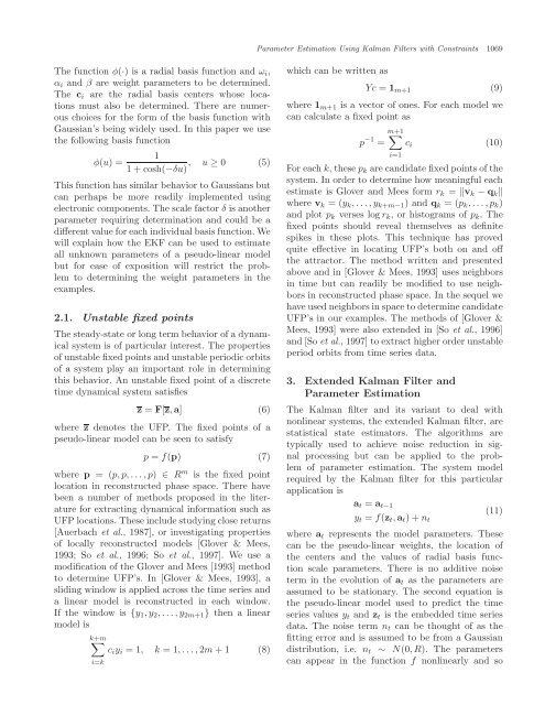
Parameter Estimation Using Kalman Filters with Constraints 1069The function φ(·) is a radial basis function and ω i ,α i and β are weight parameters to be determined.The c i are the radial basis centers whose locationsmust also be determined. There are numerouschoices for the form of the basis function withGaussian’s being widely used. In this paper we usethe following basis function1φ(u) =1+cosh(−δu) , u ≥ 0 (5)This function has similar behavior to Gaussians butcan perhaps be more readily implemented usingelectronic components. The scale factor δ is anotherparameter requiring determination and could be adifferent value for each individual basis function. Wewill explain how the EKF can be used to estimateall unknown parameters of a pseudo-linear modelbut for ease of exposition will restrict the problemto determining the weight parameters in theexamples.2.1. Unstable fixed pointsThe steady-state or long term behavior of a dynamicalsystem is of particular interest. The propertiesof unstable fixed points and unstable periodic orbitsof a system play an important role in determiningthis behavior. An unstable fixed point of a discretetime dynamical system satisfiesz = F[z, a] (6)where z denotes the UFP. The fixed points of apseudo-linear model can be seen to satisfyp = f(p) (7)where p = (p,p,...,p) ∈ R m is the fixed pointlocation in reconstructed phase space. There havebeen a number of methods proposed in the literaturefor extracting dynamical information such asUFP locations. These include studying close returns[Auerbach et al., 1987], or investigating propertiesof locally reconstructed models [Glover & Mees,1993; So et al., 1996; So et al., 1997]. We use amodification of the Glover and Mees [1993] methodto determine UFP’s. In [Glover & Mees, 1993], asliding window is applied across the time series anda linear model is reconstructed in each window.If the window is {y 1 ,y 2 ,...,y 2m+1 } then a linearmodel isk+m∑i=kc i y i =1, k =1,...,2m +1 (8)which can be written asYc = 1 m+1 (9)where 1 m+1 is a vector of ones. For each model wecan calculate a fixed point asp −1 =m+1∑i=1c i (10)For each k,thesep k are candidate fixed points of thesystem. In order to determine how meaningful eachestimate is Glover and Mees form r k = ‖v k − q k ‖where v k =(y k ,...,y k+m−1 )andq k =(p k ,...,p k )and plot p k verses log r k , or histograms of p k .Thefixed points should reveal themselves as definitespikes in these plots. This technique has provedquite effective in locating UFP’s both on and offthe attractor. The method written and presentedabove and in [Glover & Mees, 1993] uses neighborsin time but can readily be modified to use neighborsin reconstructed phase space. In the sequel wehave used neighbors in space to determine candidateUFP’s in our examples. The methods of [Glover &Mees, 1993] were also extended in [So et al., 1996]and [So et al., 1997] to extract higher order unstableperiod orbits from time series data.3. Extended Kalman Filter andParameter EstimationThe Kalman filter and its variant to deal withnonlinear systems, the extended Kalman filter, arestatistical state estimators. The algorithms aretypically used to achieve noise reduction in signalprocessing but can be applied to the problemof parameter estimation. The system modelrequired by the Kalman filter for this particularapplication isa t = a t−1(11)y t = f(z t , a t )+n twhere a t represents the model parameters. Thesecan be the pseudo-linear weights, the location ofthe centers and the values of radial basis functionscale parameters. There is no additive noiseterm in the evolution of a t as the parameters areassumed to be stationary. The second equation isthe pseudo-linear model used to predict the timeseries values y t and z t is the embedded time seriesdata. The noise term n t can be thought of as thefitting error and is assumed to be from a Gaussiandistribution, i.e. n t ∼ N(0,R). The parameterscan appear in the function f nonlinearly and so