Chapter 4 SEGMENTATION

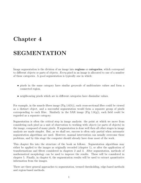
Chapter 4SEGMENTATIONImage segmentation is the division of an image into regions or categories, which correspondto different objects or parts of objects. Every pixel in an image is allocated to one of a numberof these categories. A good segmentation is typically one in which:• pixels in the same category have similar greyscale of multivariate values and form aconnected region,• neighbouring pixels which are in different categories have dissimilar values.For example, in the muscle fibres image (Fig 1.6(b)), each cross-sectional fibre could be viewedas a distinct object, and a successful segmentation would form a separate group of pixelscorresponding to each fibre. Similarly in the SAR image (Fig 1.8(g)), each field could beregarded as a separate category.Segmentation is often the critical step in image analysis: the point at which we move fromconsidering each pixel as a unit of observation to working with objects (or parts of objects) inthe image, composed of many pixels. If segmentation is done well then all other stages in imageanalysis are made simpler. But, as we shall see, success is often only partial when automaticsegmentation algorithms are used. However, manual intervention can usually overcome theseproblems, and by this stage the computer should already have done most of the work.This chapter fits into the structure of the book as follows. Segmentation algorithms mayeither be applied to the images as originally recorded (chapter 1), or after the application oftransformations and filters considered in chapters 2 and 3. After segmentation, methods ofmathematical morphology can be used to improve the results. These will be considered inchapter 5. Finally, in chapter 6, the segmentation results will be used to extract quantitativeinformation from the images.There are three general approaches to segmentation, termed thresholding, edge-based methodsand region-based methods.1

2 CHAPTER 4. SEGMENTATION• In thresholding, pixels are allocated to categories according to the range of values inwhich a pixel lies. Fig 4.1(a) shows boundaries which were obtained by thresholding themuscle fibres image. Pixels with values less than 128 have been placed in one category,and the rest have been placed in the other category. The boundaries between adjacentpixels in different categories has been superimposed in white on the original image. It canbe seen that the threshold has successfully segmented the image into the two predominantfibre types.• In edge-based segmentation, an edge filter is applied to the image, pixels are classifiedas edge or non-edge depending on the filter output, and pixels which are not separated byan edge are allocated to the same category. Fig 4.1(b) shows the boundaries of connectedregions after applying Prewitt’s filter (§3.4.2) and eliminating all non-border segmentscontaining fewer than 500 pixels. (More details will be given in §4.2.)• Finally, region-based segmentation algorithms operate iteratively by grouping togetherpixels which are neighbours and have similar values and splitting groups of pixels whichare dissimilar in value. Fig 4.1(c) shows the boundaries produced by one such algorithm,based on the concept of watersheds, about which we will give more details in §4.3.Note that none of the three methods illustrated in Fig 4.1 has been completely successful insegmenting the muscle fibres image by placing a boundary between every adjacent pair of fibres.Each method has distinctive faults. For example, in Fig 4.1(a) boundaries are well placed, butothers are missing. In Fig 4.1(c), however, more boundaries are present, and they are smooth,but they are not always in exactly the right positions.The following three sections will consider these three approaches in more detail. Algorithmswill be considered which can either be fully automatic or require some manual intervention.The key points of the chapter will be summarized in §4.4.4.1 ThresholdingThresholding is the simplest and most commonly used method of segmentation. Given a singlethreshold, t, the pixel located at lattice position (i, j), with greyscale value f ij , is allocated tocategory 1 iff ij ≤ t.Otherwise, the pixel is allocated to category 2.In many cases t is chosen manually by the scientist, by trying a range of values of t and seeingwhich one works best at identifying the objects of interest. Fig 4.2 shows some segmentationsof the soil image. In this application, the aim was to isolate soil material from the air-filledpores which appear as the darker pixels in Fig 1.6(c). Thresholds of 7, 10, 13, 20, 29 and 38were chosen in Figs 4.2(a) to (f) respectively, to identify approximately 10, 20, 30, 40, 50 and60% of the pixels as being pores. Fig 4.2(d), with a threshold of 20, looks best because most

4.1. THRESHOLDING 3(a)(b)(c)Figure 4.1: Boundaries produced by three segmentations of the muscle fibres image: (a) bythresholding, (b) connected regions after thresholding the output of Prewitt’s edge filter andremoving small regions, (c) result produced by watershed algorithm on output from a variancefilter with Gaussian weights (σ 2 = 96).

4 CHAPTER 4. SEGMENTATION(a)(b)(c)(d)(e)(f)Figure 4.2: Six segmentations of the soil image, obtained using manually-selected thresholdsof (a) 7, (b) 10, (c) 13, (d) 20, (e) 29 and (f) 38. These correspond to approximately10%, 20%,...,60%, respectively, of the image being displayed as black.

4.1. THRESHOLDING 5of the connected pore network evident in Fig 1.6(c) has been correctly identified, as has mostof the soil matrix.Note that:• Although pixels in a single thresholded category will have similar values (either in therange 0 to t, or in the range (t + 1) to 255), they will not usually constitute a singleconnected component. This is not a problem in the soil image because the object (air)is not necessarily connected, either in the imaging plane or in three-dimensions. In othercases, thresholding would be followed by dividing the initial categories into sub-categoriesof connected regions.• More than one threshold can be used, in which case more than two categories are produced.• Thresholds can be chosen automatically.In §4.1.1 we will consider algorithms for choosing the threshold on the basis of the histogramof greyscale pixel values. In §4.1.2, manually- and automatically-selected classifiers for multivariateimages will be considered. Finally, in §4.1.3, thresholding algorithms which make useof context (that is, values of neighbouring pixels as well as the histogram of pixel values) willbe presented.4.1.1 Histogram-based thresholdingWe will denote the histogram of pixel values by h 0 ,h 1 ,...,h N , where h k specifies the numberof pixels in an image with greyscale value k and N is the maximum pixel value (typically255). Ridler and Calvard (1978) and Trussell (1979) proposed a simple algorithm for choosinga single threshold. We shall refer to it as the intermeans algorithm. First we will describethe algorithm in words, and then mathematically.Initially, a guess has to be made at a possible value for the threshold. From this, the mean valuesof pixels in the two categories produced using this threshold are calculated. The thresholdis repositioned to lie exactly half way between the two means. Mean values are calculatedagain and a new threshold is obtained, and so on until the threshold stops changing value.Mathematically, the algorithm can be specified as follows.1. Make an initial guess at t: for example, set it equal to the median pixel value, that is,the value for whicht∑h k ≥ n2t−12 > ∑h k ,k=0k=0where n 2 is the number of pixels in the n × n image.

4.1. THRESHOLDING 7The intermeans algorithm has a tendency to find a threshold which divides the histogram intwo, so that there are approximately equal numbers of pixels in the two categories. In manyapplications, such as the soil image, this is not appropriate. One way to overcome this drawbackis to modify the algorithm as follows.Consider a distribution which is a mixture of two Gaussian distributions. Therefore, in theabsence of sampling variability, the histogram is given by:h k = n 2 {p 1 φ 1 (k)+p 2 φ 2 (k)},for k =0, 1,...,N.Here, p 1 and p 2 are proportions (such that p 1 + p 2 = 1) and φ l (k) denotes the probabilitydensity of a Gaussian distribution, that is{ }1 −(k − µl ) 2φ l (k) = √ expfor l =1, 2,2πσ2lwhere µ l and σl2 are the mean and variance of pixel values in category l. The best classificationcriterion, i.e. the one which misclassifies the least number of pixels, allocates pixels with valuek to category 1 ifp 1 φ 1 (k) ≥ p 2 φ 2 (k),and otherwise classifies them as 2. After substituting for φ and taking logs, the inequalitybecomes { 1k 2 − 1 } {µ1− 2k − µ } { }2 µ2+ 1− µ2 2+ log σ2 1p 2 2≤ 0.σ12 σ22 σ12 σ22 σ12 σ22 σ2p 2 2 1The left side of the inequality is a quadratic function in k. Let A, B and C denote the threeterms in curly brackets, respectively. Then the criterion for allocating pixels with value k tocategory 1 is:k 2 A − 2kB + C ≤ 0.There are three cases to consider:(a) If A = 0 (i.e. σ1 2 = σ2 2 ), the criterion simplifies to one of allocating pixels with value k tocategory 1 if2kB ≥ C.(If, in addition, p 1 = p 2 and µ 1

8 CHAPTER 4. SEGMENTATIONThe criteria for category 1 aret 1 t 2if A>0,if A

10 CHAPTER 4. SEGMENTATIONa greater overall brightness than others. Alternatively, trend can sometimes be removedbefore thresholding an image, for example by using a top-hat transform (§5.5).4.1.2 Multivariate classifiersThere are many ways to extend the concept of a threshold in order to segment a multivariateimage, such as:• Allocate pixel (i, j) to category 1 iff ij,m ≤ t mfor m =1,...,M,where subscript m denotes the variate number, and there are M variates.• Or, more generally, use a box classifier where the conditions for category 1 are:t 1,m

4.1. THRESHOLDING 11where summation is over all the N r pixels in region B r . The simplest case to consider is wherethe variance-covariance matrices in the different categories are assumed to be the same. In thiscase, the common variance-covariance matrix, V , can be estimated as⎛⎞R∑V = ⎝ ∑∑/∑ RTf ij f ij − N r µ r µ T ⎠r N r .r=1(i,j)∈B rDistances in multidimensional space are measured taking into account the variance-covariancematrix V . The squared Mahalanobis distance between pixel value f ij and the rth categorymean is(f ij − µ r ) T V −1 (f ij − µ r ),where the superscript ‘−1’ denotes a matrix inverse.The segmentation rule is to allocate each pixel in the image to the nearest category mean, asmeasured by the above distance. The rule simplifies to a set of linear thresholds. For example,in the two category case, a pixel is allocated to category 1 ifr=1µ T 1 V −1 µ 1 − 2µ T 1 V −1 f ij ≤ µ T 2 V −1 µ 2 − 2µ T 2 V −1 f ij .This is linear discrimination. If the variances are not assumed to be equal, then this resultsin quadratic discrimination. For more details, see for example Krzanowski (1988, §12.2).Fig 4.5 shows this method applied to the bivariate image obtained by combining the MRIproton density and inversion recovery images of a woman’s chest (Figs 1.7(a) and (b)). Fourtraining areas have been selected manually as representatives of1. lung tissue,2. blood in the heart,3. muscle, and other lean tissues,4. adipose tissues, such as subcutaneous fat.These areas are shown superimposed on the inversion recovery and proton density images inFigs 4.5(a) and (b).Fig 4.5(c) is a scatter plot of f ij,2 against f ij,1 for the training pixels, together with the linearseparators of all pixel values into the four classes. For example, the muscle pixels are placed inthe top-left of Fig 4.5(c) because they have high values of proton density but low values fromthe inversion recovery signal, as can be seen in Figs 4.5(a) and (b). The points have been codedin progressively darker shades of grey, to denote lung, muscle, blood and fat pixels respectively.There is substantial overlap between blood and fat pixels in Fig 4.5(c), so that even the trainingset has not been classified precisely.Fig 4.5(d) shows the pixel allocation of the whole image. Air pixels, for which f ij = 0, havebeen excluded from all classes. The lungs, shown as the lightest shade of grey, have been

12 CHAPTER 4. SEGMENTATION(a)(b)(c)(d)Figure 4.5: Manual segmentation of the bivariate MRI image: (a) inversion recovery imagewith boundaries of 4 training areas superimposed — these are, from left to right, lung tissue,moving blood, muscle and subcutaneous fat; (b) proton density image with the same trainingareas shown; (c) scatter plot of values of training pixels, and linear discrimination classification,with points displayed in increasing levels of darkness for lung pixels, muscle, blood and fat; (d)segmentation of image by linear discrimination, using the same greyscale as in (c).

14 CHAPTER 4. SEGMENTATION(a)(b)(c)(d)(e)(f)Figure 4.6: Automatic segmentations of the MRI image into 2, 3 and 4 classes: (a) bivariatehistogram of pixel values, together with centres of two clusters and the division between themobtained by k-means clustering, (b) result displayed as an image, (c) bivariate histogram andoptimal division into 3 clusters, and (d) image display, (e) bivariate histogram and optimaldivision into 4 clusters, and (f) image display.

16 CHAPTER 4. SEGMENTATIONFigure 4.7: Histograms of muscle fibres image: (a) original pixel values, displayed on a squarerootscale; (b) image after smoothing by Gaussian filter (σ 2 =6 2 ); (c) bivariate histogram of3original pixel values and those after smoothing, with all counts exceeding 25 displayed as blackand the parallel diagonal lines indicating the points extracted for (d); (d) histogram of pixelvalues after smoothing those values within 5 of those before smoothing, the arrows indicate thethresholds used in Fig 4.8.

4.1. THRESHOLDING 17Figure 4.8: Thresholded muscle fibres image. Pixels in the range 0 to 50 and 166 to 255 aredisplayed as white, those between 51 and 90 are black, between 91 and 130 they are dark greyand between 131 and 165 they are shown as light grey.histogram from non-edge pixels only, its peaks should be clearer.Another way of using contextual information is by applying a majority filter to a segmentedimage, termed post-classification smoothing. For example, if pixel (i, j) has been labelledas category g ij by a segmentation algorithm, then a majority filter relabels (i, j) asthe most common category in a (2m +1)× (2m + 1) window centred on pixel (i, j), i.e. the set{g i+k,j+l for k, l = −m,...,m}.Contextual information can also be used in automatic segmentation algorithms. Mardia andHainsworth (1988) investigated incorporating post-classification smoothing into a thresholdingalgorithm. (Their paper also provides a succinct review of algorithms for thresholding imageswhose pixel values are mixtures of Gaussian distributions.) To explain the method, we willconsider the simplest case. First we will discuss it in words, and then more formally.From an initial guess at a threshold, an image is segmented. Then the classified image issmoothed using a majority filter, so that neighbouring pixels are more often classified thesame. Mean pixel values are evaluated in each category and the threshold is re-estimated usingthe intermeans criterion (§4.1.1). The image is segmented and smoothed again, and so on untilthe threshold does not change between successive iterations. Formally:1. Make an initial guess at a threshold t.

18 CHAPTER 4. SEGMENTATION2. Segment the image, by thresholding, and store the result in an array g:g ij =1 iff ij ≤ t, otherwise g ij =2.3. Apply a majority filter to g, and record the new labels in array g ′ . Therefore, g ′ ij is setto the most common category in the set {g i+k,j+l for k, l = −m,...,m}. This is repeatedfor every value of i and j from (m +1)to(n − m). (Ranges having been chosen to avoidimage borders, as in chapter 3.)4. Calculate the mean pixel value in category 1,µ 1 = 1 N 1∑∑{(i,j) such that g ′ ij =1} f ij ,where N 1 is the number of pixels in category 1. Similarly, calculate µ 2 .5. Re-estimate t as [ 1 2 (µ 1 + µ 2 )].6. Repeat steps (2) to (5) until t converges to a stable value, and then stop after step (3).Fig 4.9(b) shows the segmentation of the log-transformed SAR image (as shown in Fig 2.6)into two classes using the above algorithm and a 5 × 5 smoothing window. The algorithmconverged in four iterations, starting with a threshold set at the median pixel value. Thewindow size was chosen by trial-and-error: a size less than 5 × 5 was inadequate for smoothingthe inconsistencies in classification caused by the noise, whereas a larger size produced an oversmoothsegmentation — corners of fields became rounded. Fig 4.9(a) shows the result of thesame algorithm without smoothing — that is, the intermeans algorithm. The noise is so greatin this image that the histogram of pixel values is unimodal and no threshold can achieve abetter segmentation.Mardia and Hainsworth compared their algorithm with a simple form of Bayesian imagerestoration, which uses Besag’s (1986) iterated conditional modes (ICM) algorithm. Wewill consider the simplest case of ICM, first in words and then formally.From an initial guess at a threshold, or equivalently of the two category means, the image issegmented. Mean pixel values are evaluated in each category and the image is re-segmented,pixel by pixel, using a variable threshold which takes account both of the category means andof the current classification of neighbouring pixels. Category means are recalculated and therecursive segmentation procedure is re-applied. These steps are repeated until the segmentationremains (almost) unchanged on successive iterations. More formally:1. Make an initial guess at µ 1 and µ 2 , and setOr equivalently,g ij = 1 if (f ij − µ 1 ) 2 ≤ (f ij − µ 2 ) 2 , otherwise g ij =2.[ ]µ1 + µ 2g ij =1 iff ij ≤ t, where t = .2

4.1. THRESHOLDING 19(a)(b)(c)Figure 4.9: Three segmentations of the log-transformed SAR image: (a) obtained by thresholdingusing the intermeans algorithm, (b) thresholding combined with a post-classificationsmoothing by majority filter in a 5 × 5 window, (c) iterated conditioned modes (ICM) classification,with β =1.5.

20 CHAPTER 4. SEGMENTATION2. Calculate the mean pixel values in the two categories, µ 1 and µ 2 . Also calculate thewithin-category varianceσ 2 = 1 n∑ n∑(fn 2ij − µ gij ) 2 .i=13. Re-segment, recursively, as follows. For each value of i between 1 and n apply the followingcriterion in turn for j between 1 and n:j=1g ij = 1 if (f ij − µ 1 ) 2 − βσ 2 N ij ≤ (f ij − µ 2 ) 2 − βσ 2 (8 − N ij ),where N ij is the number of the eight neighbours of pixel (i, j), currently classified as 1and β is a constant whose value must be chosen. A value of 1.5 has often been used inthe literature.Equivalently, this reclassification be viewed as a variable threshold:[ (µ1 + µ 2 )g ij =1 iff ij ≤ t ij , where t ij =2+ βσ2 (2N ij − 8)2(µ 2 − µ 1 )Note that (i−1,j−1), (i−1,j), (i−1,j+1) and (i, j −1) will have already been updated,although alternatively, all pixels can be reclassified simultaneously. The two approachesare termed asynchronous and synchronous, respectively.4. Repeat steps (2) and (3) until no (or only a few) pixels change category.].Fig 4.9(c) shows the results of applying the ICM algorithm to the SAR image. In this case,20 iterations were performed, by which stage fewer than 5 pixels changed classes betweeniterations. The final segmentation is very similar to that produced by applying the majorityfilter, shown in Fig 4.9(b). Mardia and Hainsworth (1988) also found that the two algorithmsoften gave very similar results.The ICM algorithm is a very simple example of Bayesian image restoration — a potentiallypowerful technique which has received much attention from statisticians in the last decade,following seminal papers by Geman and Geman (1984) and Besag (1986). The underlyingprinciple is that of combiningprior information on what the segmented image should be like, anddata, the observed pixel values in an image,in order to produce a segmentation. In our example, the term βN ij is motivated by a MarkovRandom Field model, and favours a segmentation in which neighbouring pixels are classifiedthe same. The main attraction of Bayesian image restoration is that it is open to manyrefinements, such as incorporating more specific prior information. However, computational feasibilityof Bayesian restoration algorithms can be a limiting factor. See, for example, Aykroydand Green (1991), Ripley and Sutherland (1990) and Qian and Titterington (1991) for a rangeof applications.

4.2. EDGE-BASED SEGMENTATION 21(a)(b)Figure 4.10: (a) Boundaries obtained by thresholding the muscle fibres image, superimposedon output for Prewitt’s filter, with values between 0 and 5 displayed in progressively darkershades of grey and values in excess of 5 displayed as black. (b) Manual segmentation of theimage by addition of extra lines to boundaries obtained by thresholding, superimposed in whiteon the original image.4.2 Edge-based segmentationAs we have seen, the results of threshold-based segmentation are usually less than perfect.Often, a scientist will have to make changes to the results of automatic segmentation. Onesimple way of doing this is by using a computer mouse to control a screen cursor and drawboundary lines between regions. Fig 4.10(a) shows the boundaries obtained by thresholdingthe muscle fibres image (as already displayed in Fig 4.1(a)), superimposed on the output fromPrewitt’s edge filter (§3.4.2), with the contrast stretched so that values between 0 and 5 aredisplayed as shades of grey ranging from white to black and values exceeding 5 are all displayedas black. This display can be used as an aid to determine where extra boundaries need to beinserted to fully segment all muscle fibres. Fig 4.10(b) shows the result after manually adding71 straight lines.Algorithms are available for semi-automatically drawing edges, whereby the scientist’s roughlines are smoothed and perturbed to maximise some criterion of match with the image (see, forexample, Samadani and Han, 1993). Alternatively, edge finding can be made fully automatic,although not necessarily fully successful. Fig 4.11(a) shows the result of applying Prewitt’sedge filter to the muscle fibre image. In this display, the filter output has been thresholded at avalue of 5: all pixels exceeding 5 are labelled as edge pixels and displayed as black. Connectedchains of edge pixels divide the image into regions. Segmentation can be achieved by allocatingto a single category all non-edge pixels which are not separated by an edge. Rosenfeld and

22 CHAPTER 4. SEGMENTATION(a)(b)Figure 4.11: (a) Thresholded output from Prewitt’s edge filter applied to muscle fibres image:values greater than 5 are displayed as black, those less than or equal to 5 as white. (b)Boundaries produced from connected regions in (a), superimposed in white on the originalimage.Pfaltz (1966) gave an efficient algorithm for doing this for 4- and 8-connected regions, termeda connected components algorithm. We will describe this algorithm in words, and thenmathematically.The algorithm operates on a raster scan, in which each pixel is visited in turn, starting atthe top-left corner of the image and scanning along each row, finishing at the bottom-rightcorner. For each non-edge pixel, (i, j), the following conditions are checked. If its alreadyvisitedneighbours — (i − 1,j) and (i, j − 1) in the 4-connected case, also (i − 1,j − 1) and(i − 1,j+ 1) in the 8-connected case — are all edge pixels, then a new category is created and(i, j) is allocated to it. Alternatively, if all its non-edge neighbours are in a single category,then (i, j) is also placed in that category. The final possibility is that neighbours belong to twoor more categories, in which case (i, j) is allocated to one of them and a note is kept that thesecategories are connected and therefore should from then on be considered as a single category.More formally, for the simpler case of 4-connected regions:• Initialize the count of the number of categories by setting K =0.• Consider each pixel (i, j) in turn in a raster scan, proceeding row by row (i =1,...,n),and for each value of i taking j =1,...,n.• One of four possibilities apply to pixel (i, j):1. If (i, j) is an edge pixel then nothing needs to be done.

4.2. EDGE-BASED SEGMENTATION 232. If both previously-visited neighbours, (i − 1,j) and (i, j − 1), are edge pixels, thena new category has to be created for (i, j):K → K +1, h K = K, g ij = K,where the entries in h 1 ,...,h K are used to keep track of which categories are equivalent,and g ij records the category label for pixel (i, j).3. If just one of the two neighbours is an edge pixel, then (i, j) is assigned the samelabel as the other one:{gi−1,j if (i, j − 1) is the edge pixel,g ij =otherwise.g i,j−14. The final possibility is that neither neighbour is an edge pixel, in which case (i, j) isgiven the same label as one of them:g ij = g i−1,j ,and if the neighbours have labels which have not been marked as equivalent, i.e.h gi−1,j ≠ h gi,j−1 , then this needs to be done (because they are connected at pixel(i, j)). The equivalence is recorded by changing the entries in h 1 ,...,h K , as follows:– Set l 1 = min(h gi−1,j ,h gi,j−1 ) and l 2 = max(h gi−1,j ,h gi,j−1 ).– For each value of k from 1 to K, ifh k = l 2 then h k → l 1 .• Finally, after all the pixels have been considered, the array of labels is revised, taking intoaccount which categories have been marked for amalgamation:g ij → h gijfor i, j =1,...,n.After application of the labelling algorithm, superfluous edge pixels — that is, those whichdo not separate classes — can be removed: any edge-pixel which has neighbours only of onecategory is assigned to that category.Fig 4.11(b) shows the result of applying the labelling algorithm with edges as shown in Fig 4.11(a),and removing superfluous edge pixels. The white boundaries have been superimposed on theoriginal image. Similarly, small segments (say less than 500 pixels in size) which do not touchthe borders of the image can be removed, leading to the previously displayed Fig 4.1(b). Thesegmentation has done better than simple thresholding, but has failed to separate all fibres becauseof gaps in output from Prewitt’s edge filter. Martelli (1976), among others, has proposedalgorithms for bridging these gaps.Another edge-detection filter considered in chapter 3 was the Laplacian-of-Gaussian (§3.1.2).This filter can also be used to segment images, using the zero-crossings of the output to specifypositions of boundaries. One advantage over Prewitt’s filter is that the zero-crossings alwaysform closed boundaries. Fig 4.12(a) shows output from the Laplacian-of-Gaussian filter

24 CHAPTER 4. SEGMENTATION(a)(b)Figure 4.12: (a) Output from Laplacian-of-Gaussian filter (σ 2 = 27) applied to muscle fibresimage. (b) Zero-crossings from (a) with average image gradients in excess of 1.0, in whitesuperimposed on the image.(σ 2 = 27), applied to the muscle fibres image. Boundaries corresponding to weak edges canbe suppressed by applying a threshold to the average gradient strength around a boundary.Fig 4.12(b) shows zero-crossings of the Laplacian-of-Gaussian filter with average gradients exceedingunity, superimposed on the original image. In this application the result can be seento be little better than simple thresholding.4.3 Region-based segmentationSegmentation may be regarded as spatial clustering:• clustering in the sense that pixels with similar values are grouped together, and• spatial in that pixels in the same category also form a single connected component.Clustering algorithms may be agglomerative, divisive or iterative (see, for example, Gordon,1981). Region-based methods can be similarly categorized into:• those which merge pixels,• those which split the image into regions, and

4.3. REGION-BASED SEGMENTATION 25• those which both split-and-merge in an iterative search scheme.The distinction between edge-based and region-based methods is a little arbitrary. For example,in §4.2 one of the algorithms we considered involved placing all neighbouring non-edge pixelsin the same category. In essence, this is a merging algorithm.Seeded region growing is a semi-automatic method of the merge type. We will explain it byway of an example. Fig 4.13(a) shows a set of seeds, white discs of radius 3, which have beenplaced inside all the muscle fibres, using an on-screen cursor controlled by a computer mouse.Fig 4.13(b) shows again the output from Prewitt’s edge filter. Superimposed on it in white arethe seeds and the boundaries of a segmentation produced by a form of watershed algorithm.The boundaries are also shown superimposed on the original muscle fibres image in Fig 4.13(c).The watershed algorithm operates as follows (we will explain the name later).For each of a sequence of increasing values of a threshold, all pixels with edge strength lessthan this threshold which form a connected region with one of the seeds are allocated to thecorresponding fibre. When a threshold is reached for which two seeds become connected, thepixels are used to label the boundary. A mathematical representation of the algorithm is toocomplicated to be given here. Instead, we refer the reader to Vincent and Soille (1991) formore details and an efficient algorithm. Meyer and Beucher (1990) also consider the watershedalgorithm, and added some refinements to the method.Note that:• The use of discs of radius 3 pixels, rather than single points, as seeds make the watershedresults less sensitive to fluctuations in Prewitt’s filter output in the middle of fibres.• The results produced by this semi-automatic segmentation algorithm are almost as goodas those shown in Fig 4.10(b), but the effort required in positioning seeds inside musclefibres is far less than that required to draw boundaries.• Adams and Bischof (1994) present a similar seeded region growing algorithm, but baseddirectly on the image greyscale, not on the output from an edge filter.Th watershed algorithm, in its standard use, is fully automatic. Again, we will demonstrate thisby illustration. Fig 4.14 shows the output produced by a variance filter (§3.4.1) with Gaussianweights (σ 2 = 96) applied to the muscle fibres image after histogram-equalization (as shownin Fig 2.7(d)). The white seeds overlie all the local minima of the filter output, that is, pixelswhose neighbours all have larger values and so are shaded lighter. Note that it is necessary touse a large value of σ 2 to ensure that the filter output does not have many more local minima.The boundaries produced by the watershed algorithm have been added to Fig 4.14. An intuitiveway of viewing the watershed algorithm is by considering the output from the variance filter asan elevation map: light areas are high ridges and dark areas are valleys (as in Fig 1.5). Eachlocal minimum can be thought of as the point to which any water falling on the region drains,and the segments are the catchments for them. Hence, the boundaries, or watersheds, lie alongtops of ridges. The previously mentioned Fig 4.1(c) shows this segmentation superimposed onthe original image.

26 CHAPTER 4. SEGMENTATION(a)(b)(c)Figure 4.13: Manual segmentation of muscle fibres image by use of watersheds algorithm:(a) manually positioned ‘seeds’ in centres of all fibres, (b) output from Prewitt’s edge filter,together with watershed boundaries, (c) watershed boundaries superimposed on the image.

4.3. REGION-BASED SEGMENTATION 27Figure 4.14: Output of variance filter with Gaussian weights (σ 2 = 96) applied to muscle fibresimage, together with seeds indicating all local minima and boundaries produced by watershedalgorithm.There are very many other region-based algorithms, but most of them are quite complicated.In this section we will consider just one more, namely an elegant split-and-merge algorithmproposed by Horowitz and Pavlidis (1976). We will present it in a slightly modified form tosegment the log-transformed SAR image (Fig 2.6), basing our segmentation decisions on variances,whereas Horowitz and Pavlidis based theirs on the range of pixel values. The algorithmoperates in two stages, and requires a limit to be specified for the maximum variance in pixelvalues in a region.The first stage is the splitting one. Initially, the variance of the whole image is calculated.If this variance exceeds the specified limit, then the image is subdivided into four quadrants.Similarly, if the variance in any of these four quadrants exceeds the limit it is further subdividedinto four. This continues until the whole image consists of a set of squares of varying sizes, allof which have variances below the limit. (Note that the algorithm must be capable of achievingthis because at the finest resolution of each square consisting of a single pixel the variances aretaken to be zero.)Fig 4.15(a) shows the resulting boundaries in white, superimposed on the log-transformed SARimage, with the variance limit set at 0.60. Note that:• Squares are smaller in non-uniform parts of the image.

28 CHAPTER 4. SEGMENTATION(a)(b)Figure 4.15: Region-growing segmentation of log-transformed SAR image: (a) division of imageinto squares with variance less than 0.60, obtained as first step in algorithm, (b) finalsegmentation, after amalgamation of squares, subject to variance limit of 0.60.• The variance limit was set to 0.60, rather than to the speckle variance value of 0.41(Horgan, 1994), because in the latter case the resulting regions were very small.• The algorithm requires the image dimension, n, to be a power of 2. Therefore, the250 × 250 SAR image was filled out to 256 × 256 by adding borders of width 3.The second stage of the algorithm, the merging one, involves amalgamating squares which havea common edge, provided that by so doing the variance of the new region does not exceed thelimit. Once all amalgamations have been completed, the result is a segmentation in which everyregion has a variance less than the set limit. However, although the result of the first stagein the algorithm is unique, that from the second is not — it depends on the order of whichsquares are considered.Fig 4.15(b) shows the boundaries produced by the algorithm, superimposed on the SAR image.Dark and light fields appear to have been successfully distinguished between, although theboundaries are rough and retain some of the artefacts of the squares in Fig 4.15(a).Pavlidis and Liow (1990) proposed overcoming the deficiencies in the boundaries produced bythe Horowitz and Pavlidis algorthm by combining the results with those from an edge-basedsegmentation. Many other ideas for region-based segmentation have been proposed (see, forexample, the review of Haralick and Shapiro, 1985), and it is still an active area of research.

4.4. SUMMARY 29One possibility for improving segmentation results is to use an algorithm which over-segmentsan image, and then apply a rule for amalgamating these regions. This requires ‘high-level’knowledge, which falls into the domain of artificial intelligence. (All that we have consideredin this chapter may be termed ‘low-level’.) For applications of these ideas in the area ofremote sensing, see Tailor, Cross, Hogg and Mason (1986) and Ton, Sticklen and Jain (1991).It is possible that such domain-specific knowledge could be used to improve the automaticsegmentations of the SAR and muscle fibres images, for example by constraining boundaries tobe straight in the SAR image and by looking only for convex regions of specified size for themuscle fibres.We briefly mention some other, more-complex techniques which can be used to segment images.• The Hough transform (see, for example, Leavers, 1992) is a powerful technique forfinding straight lines, and other parametrized shapes, in images.• Boundaries can be constrained to be smooth by employing roughness penalties such asbending energies. The approach of varying a boundary until some such criterion is optimizedis known as the fitting of snakes (Kass, Witkin and Terzopoulos 1988).• Models of expected shapes can be represented as templates and matched to images.Either the templates can be rigid and the mapping can be flexible (for example, the thinplatespline of Bookstein, 1989), or the template itself can be flexible, as in the approachof Amit, Grenander and Piccioni (1991).• Images can be broken down into fundamental shapes, in a way analogous to the decompositionof a sentence into individual words, using syntactic methods (Fu, 1974).4.4 SummaryThe key points about image segmentation are:• Segmentation is the allocation of every pixel in an image to one of a number of categories,which correspond to objects or parts of objects. Commonly, pixels in a single categoryshould:– have similar pixel values,– form a connected region in the image,– be dissimilar to neighbouring pixels in other categories.• Segmentation algorithms may either be applied to the original images, or after the applicationof transformations and filters (considered in chapters 2 and 3).• Three general approaches to segmentation are:

30 CHAPTER 4. SEGMENTATION– thresholding,– edge-based methods,– region-based methods.• Methods within each approach may be further divided into those which:– require manual intervention, or– are fully automatic.A single threshold, t, operates by allocating pixel (i, j) to category 1 if f ij ≤ t, and otherwiseputting it in category 2. Thresholds may be obtained by:• manual choice, or• applying an algorithm such as intermeans or minimum-error to the histogram of pixelvalues.– Intermeans positions t half-way between the means in the two categories.– Minimum-error chooses t to minimize the total number of misclassifications on theassumption that pixel values in each category are Normally distributed.• Thresholding methods may also be applied to multivariate images.possibilities are:In this case, two– manually selecting a training set of pixels which are representative of the differentcategories, and then using linear discrimination,– k-means clustering, in which the categories are selected automatically from the data.• The context of a pixel, that is the values of neighbouring pixels, may also be used tomodify the threshold value in the classification process. We considered three methods:– restricting the histogram to those pixels which have similarly valued neighbours,– post-classification smoothing,– using Bayesian image restoration methods, such as the iterated conditional modes(ICM) algorithm.In edge-based segmentation, all pixels are initially labelled as either being on an edge or not,then non-edge pixels which form connected regions are allocated to the same category. Edgelabelling may be:• manual, by using a computer mouse to control a screen cursor and draw boundary linesbetween regions,

4.4. SUMMARY 31• automatic, by using an edge-detection filter. Edges can be located either:– where output from a filter such as Prewitt’s exceeds a threshold, or– at zero crossings from a Laplacian-of-Gaussian filter.Region-based algorithms act by grouping neighbouring pixels which have similar values andsplitting groups of pixels which are heterogeneous in value. Three methods were considered:• Regions may be grown from manually-positioned ‘seed’ points, for example, by applyinga watershed algorithm to output from Prewitt’s filter.• The watershed algorithm may also be run fully automatically, for example, by using localminima from a variance filter as seed points.• One split-and-merge algorithm finds a partition of an image such that the variance inpixel values within every segment is below a specified threshold, but no two adjacentsegments can be amalgamated without violating the threshold.Finally, the results from automatic segmentation can be improved by:• using methods of mathematical morphology (chapter 5).• using domain-specific knowledge, which is beyond the scope of this bookThe segmentation results will be used in chapter 6 to extract quantitative information fromimages.