Chapter 4 SEGMENTATION

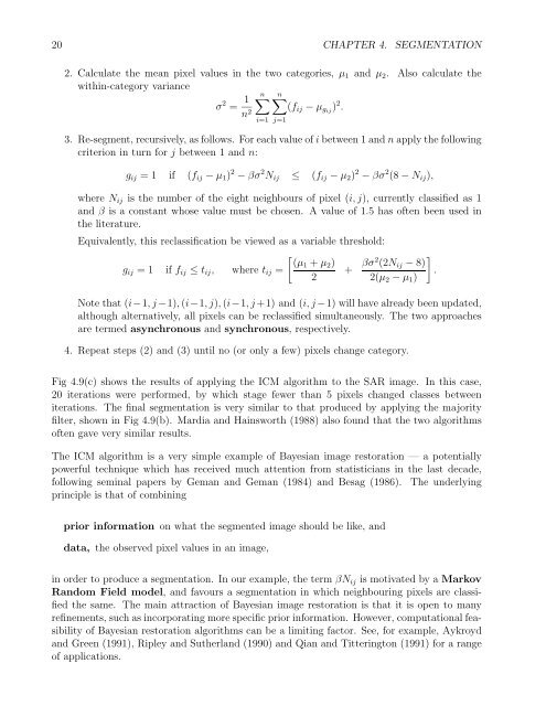
20 CHAPTER 4. SEGMENTATION2. Calculate the mean pixel values in the two categories, µ 1 and µ 2 . Also calculate thewithin-category varianceσ 2 = 1 n∑ n∑(fn 2ij − µ gij ) 2 .i=13. Re-segment, recursively, as follows. For each value of i between 1 and n apply the followingcriterion in turn for j between 1 and n:j=1g ij = 1 if (f ij − µ 1 ) 2 − βσ 2 N ij ≤ (f ij − µ 2 ) 2 − βσ 2 (8 − N ij ),where N ij is the number of the eight neighbours of pixel (i, j), currently classified as 1and β is a constant whose value must be chosen. A value of 1.5 has often been used inthe literature.Equivalently, this reclassification be viewed as a variable threshold:[ (µ1 + µ 2 )g ij =1 iff ij ≤ t ij , where t ij =2+ βσ2 (2N ij − 8)2(µ 2 − µ 1 )Note that (i−1,j−1), (i−1,j), (i−1,j+1) and (i, j −1) will have already been updated,although alternatively, all pixels can be reclassified simultaneously. The two approachesare termed asynchronous and synchronous, respectively.4. Repeat steps (2) and (3) until no (or only a few) pixels change category.].Fig 4.9(c) shows the results of applying the ICM algorithm to the SAR image. In this case,20 iterations were performed, by which stage fewer than 5 pixels changed classes betweeniterations. The final segmentation is very similar to that produced by applying the majorityfilter, shown in Fig 4.9(b). Mardia and Hainsworth (1988) also found that the two algorithmsoften gave very similar results.The ICM algorithm is a very simple example of Bayesian image restoration — a potentiallypowerful technique which has received much attention from statisticians in the last decade,following seminal papers by Geman and Geman (1984) and Besag (1986). The underlyingprinciple is that of combiningprior information on what the segmented image should be like, anddata, the observed pixel values in an image,in order to produce a segmentation. In our example, the term βN ij is motivated by a MarkovRandom Field model, and favours a segmentation in which neighbouring pixels are classifiedthe same. The main attraction of Bayesian image restoration is that it is open to manyrefinements, such as incorporating more specific prior information. However, computational feasibilityof Bayesian restoration algorithms can be a limiting factor. See, for example, Aykroydand Green (1991), Ripley and Sutherland (1990) and Qian and Titterington (1991) for a rangeof applications.