Article: Forward Scatter Radar for Future Systems

ABSTRACT 

This paper reviews the concept of a forward-scatter radar (FSR) which exploits the enhanced bistatic radar cross-section of a target in the 

forward direction (as opposed to the conventional back-scatter direction). FSR has the potential to reliably detect and track small air-vehicles 

with high sensitivity. Fundamentals of radar (including monostatic, bistatic, and multistatic) and a brief history are presented. Limitations 

of FSR radars are presented along with methods for overcoming them based on new technologies – accurate electromagnetic simulators, 

mesh networks, global positioning system (GPS) location of illuminators and receivers, and smaller and lighter transmitters and 

receivers. A program plan to accomplish these goals is given in the Appendices, along with an example of solving the target location for three 

transmitters and one receiver. 

INTRODUCTION 

In conventional radar configurations, the transmitter and receiver 

are collocated, and thus can be considered monostatic radar. Conversely, 

bistatic radar is composed of a transmitter and a receiver that 

are physically separated. Multistatic radar has transmitting and 

receiving apertures located in various positions. A recent paper 

makes it clear why a new look at multi-static systems is necessary at 

this time. 

“Compared to conventional radars, multistatic radars have the 

potential to provide significantly improved interferencerejection, 

tracking and discrimination performance in severe 

EMI and clutter environments. They can potentially provide 

significantly improved target tracking accuracy because of the 

large baseline between the various apertures. The resulting 

angular resolution can be orders of magnitude better than 

the resolution of a monolithic system (single large radar). 

The same angular resolution can provide improved interference 

rejection.”[1] 

In addition, orthogonal frequency division multiplexing 

(OFDM) can improve the performance of a radar network, 

in which each radar system would be either monostatic 

or bistatic. This configuration enables the 

classification of objects by ensuring each object is observed 

from different angles.[2] 

What is Forward Scatter Radar? 

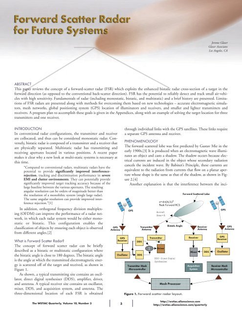
The concept of forward scatter radar can be briefly 

described as a bistatic or multistatic configuration where 

the bistatic angle is close to 180 degrees. The bistatic angle 

is the angle at which the transmitted electromagnetic energy 

is scattered off of the target and received, as shown in 

Figure 1. 

As shown, a typical transmitting site contains an oscillator, 

direct digital synthesizer (DDS), amplifier, driver, 

and antenna. A typical receiver site contains an oscillator, 

mixer, DDS, and acquisition system, and antenna. The 

three-dimensional location of each FSR is obtained 

GPS 

Antenna 

The WSTIAC Quarterly, Volume 10, Number 3 3 

http://wstiac.alionscience.com 

http://wstiac.alionscience.com/quarterly 

Jerome Glaser 

Glaser Associates 

Los Angeles, CA 

through individual links with the GPS satellites. These links require 

a separate GPS antenna and receiver. 

PHENOMENOLOGY 

The forward scattered lobe was first predicted by Gustav Mie in the 

early 1900s.[3] It is produced when an electromagnetic wave illuminates 

an object and casts a shadow. The shadow occurs because electrical 

currents are induced in the object whose secondary radiation 

cancels the incident wave. By Babinet’s Principle, these currents are 

equivalent to the radiation from currents that flow on a planar aperture 

whose shape is the same as that of the shadow, as shown in Figure 

2.[4] 

Another explanation is that the interference between the inci- 

GPS 

GPS 

Receiver DDS 

Oscillator 

DDS 

Transmitter 

Antenna 

Transmitter Mesh 

Microcontroller 

� 

�=4�(A/�) 2 

Peak Forward RCS 

Aircraft 

Area = A 

Driver 

Bistatic Angle 

Mesh Processor 

Forward Scattered Lobe 

Receiver 

Antenna 

GPS 

Transmitter Receiver GPS 

Receiver 

DDS – Direct Digital 

Synthesizer 

Figure 1. Forward scatter radar layout. 

Mixer DDS Oscillator 

Acquisition 

System 

Receiver Mesh 

Microcontroller 

GPS 

Antenna

Figure 2. Illustration of Babinet’s Principle.[5] 

dent and scattered wave front produces a wave front that is nearly 

the same as the incident wave front except for having a shadow 

region that corresponds to a “hole” in the wave front. This radiation 

is independent of the materials from which the body is made. Several 

studies have confirmed these results experimentally.[6] 

Using these principles, the radiation pattern in the forward scattered 

region is proportional to the magnitude of the two-dimensional 

complex Fourier transform of a uniform aperture shape that is the 

same shape as the shadow, as given by Equation 1.[5] 

� = 4π 

–– λ 2⏐��exp(jk – r – )dS Equation 1 

Where 

k – – Wavevector to field point, k = 2π __ λ (cos(θx), cos(θy), cos(θz)) λ – Wavelength 

k – Wavenumber, k = 2π __ λ 

– 

r – Aperture vector to x,y point 

dS – Area elements, dS = dxdy 

cos(θx), cos(θy), cos(θz) – Direction cosines 

This pattern may be computed in various ways including 

approximating the shadow shape by a polygon.[7] These relationships 

can be simplified to yield the peak radar cross section (RCS), 

�pk, of the forward scattered lobe, as given by Equation 2.[7] 

�pk = 4π ⎛�__ 2 

⎞ Equation 2 

⎝ λ⎠ Where 

�pk – Peak RCS of forward scattered lobe 

A – Shadow Area 

Similarly, the approximate angular width of the forward scattered 

lobe is determined by Equation 3.[7] 

�(degrees) = ⎛180 ___⎞ 

⎛� �⎞ 

Equation 3 

⎝ π ⎠ ⎝L 

Where 

⎠ 

L – maximum width or height of shadow 

To get an idea of the magnitudes, the peak RCS and azimuth and 

elevation beam widths at L-Band and S-Band for a sample 


unmanned vehicle can be estimated as follows. The overall length 

and width are assumed to be 5 ft (1.5m) and 2 ft (0.6m), respectively. 

The side projected area is 0.9m 2 . For L-Band (1GHz) the wavelength 

is 0.3m, and for S-Band (3GHz) the wavelength is 0.1m. 

The peak radar cross sections are: 

� � 4 � ⎛ ⎝ ⎞ 2 

⎠ 

For L-Band �s = 4 � ⎛ ⎞ 

⎝ ⎠ 

For S-Band �s = 4 � ⎛ A__ 

λ 

___ 0.9 

0.3 

___ 0.9⎞ 

⎝0.1⎠ 

2 

2 

= 113m 2 = 20.5 dBsm 

= 1018m 2 = 30.0 dBsm 

The angular widths in azimuth and elevation of the forward scattered 

beam, � AZ, � EL are then: 

As a result, it is more difficult to detect the target returns and 

avoid false-targets or interference at L-Band compared to that at S- 

Band. In addition, it is easier to locate the transmitters at L-Band 

than at S-Band. (More accurate simulation of the electromagnetic 

scattering from these aircraft can be obtained using 4NEC2, a 

method-of-moments code based on Numerical Electromagnetic 

Code (NEC) which is openly available.) 

Because of the narrowness of the forward scattered lobe, positioning 

the 3D location of transmitters with respect to the mesh 

receiver for an acceptable link margin is an important task. Figure 3 

plots the angular beamwidth of the forward scattered lobe versus the 

length of the object for 300 MHz, 1 GHz, and 3 GHz. Clearly, 

going to the lower frequency increases the width of the forward scattered 

lobe. 

Figure 4 presents a simple two-dimensional example will be presented 

in which the target’s range from the transmitter is determined 

via measurement of target’s azimuth (az) angle with respect 

Beamwidth vs Object Length for 300 MHz, 1GHz, 3GHz 

30.00 

25.00 

20.00 

15.00 

300 MHz 

10.00 

5.00 

1 GHz 

0.00 

3 GHz 

5 10 15 20 25 30 35 40 45 

Object Length (ft) 

Figure 3. Beamwidth of forward scattered lobe versus length of 

object. 

Table 1. Peak RCS of a sample unmanned vehicle at L- and S-Band.[8, 9] 

UAV Overall Width L-Band Peak L-Band Angular Widths S-Band Peak S-Band Angular Widths 

Length (ft) (ft) RCS (dBsm) Azimuth, Elevations (deg) Side RCS (dBsm) Azimuth, Elevation (deg) 

Sample Vehicle 5.0 2.0 20.5 11.4, 28.6 30.5 3.8, 9.4 

Beamwidth (deg) 

180 λ 180 λ 

θAZ � ___ ______ , θEL � ___ _____ 

π Length π Width 

For L-Band θAZ = ⎛ ⎞ 

⎝ ⎠ = 11.4 deg, θEL = ⎛ ⎞ = 28.6 deg 

⎝ ⎠ 

For S-Band �s = ⎛ ⎞ 

⎝ ⎠ = 3.8 deg, θ 180 ___ ___ 0.3 

180 ___ ___ 0.3 

π 1.5 

π 0.6 

180 ___ ___ 0.1 

EL = 

180 ___ ⎛___ 0.1⎞ 

= 9.4 deg 

π 1.5 

π ⎝0.6⎠ 


http://wstiac.alionscience.com/quarterly

Figure 4. Bistatic triangle in which constant range contours of the 

monostatic system, become ellipsoids with the receiver and transmitter 

at the foci.[10] 

to the receiver, bistatic differential range (BR), and range between 

receiver and transmitter (R1). 

∆R = c∆T = (R1 + R2) –R0 Equation 4 

R2 = ∆R __ ⎡ _______________ 

∆R + 2R0 ⎤ 

2 ⎣ ∆R + R0(1 - cos θ)⎦ 

Equation 5 

Where 

R0 – Baseline distance between transmitter and receiver 

R1,R2 – Distances from transmitter to target, target to 

receiver, respectively 

θ – Angle between baseline and line from receiver-to-target 

∆R – Distance difference between direct path signal 

∆T – Time difference between direct path signal and radar 

signal 

c – Speed of light = 3 x 10 8 m/s 

For typical values of ∆Τ = 10 -6 sec, ∆Τ = c∆Τ = 300 m, R0 = 1000 

m, az = 0 to 360°, in 5° increments. 

Using three transmitters and one receiver, the bistatic triangle 

can be solved by the method described in Reference [11]. This is 

described in Appendix I. 

HISTORICAL PERSPECTIVE AND CURRENT CHALLENGES 

Brief History of Forward Scatter Radar 

Forward scatter radar has had a long history of developments. Some 

milestone events are listed below. 

• 1922: First radar detection – demonstration of a bistatic, continuous 

wave (CW), interference radar to detect a wooden ship (Taylor 

and Young, Naval Research Laboratory (NRL)) 

• 1930: First aircraft detection – accidental detection of an aircraft 


several kilometers from the radar transmitter (Hyland, NRL) 

• 1932: Long range (50 nautical miles) aircraft detection (Taylor, 

Young, and Hyland) 

• 1950s: Development of semiactive missile seekers 

• 1960s: Development of radar to detect low-altitude, bomber aircraft 

– Brigand and Fluttar (AN/FPS-25) 

• Developments from 1970s through 2000s: 

• Survivability against antiradiation missiles (ARMs) 

• Project MAY BELL 1970 (Declassified in 1996). See Appendix 

I. 

• Enhanced performance in specific scenarios 

• Smaller, lighter, more efficient transmitters and receivers 

• GPS links 

• Silent Sentry System[12] – Uses existing FM or TV radiation 

to locate targets 

Why Forward Scatter Radar Now? 

Forward scatter radar is not a new concept, but there have been 

some significant challenges. Some primary issues with forward scatter 

radars have been outlined in literature, and these are listed 

below.[1, 2, 11] 

1. Need for cooperation between sites. In particular, wide-band 

data links are needed to allow correlation or interferometric 

detection methods to be used. 

2. Difficulty of coordinate conversion, arising from hyperbolic 

contours or constant time difference between each transmission 

and receiving station. 

3. Need for high rejection of electromagnetic interference (EMI) 

jamming and clutter that is not offered by monostatic radar. 

4. Use of orthogonal frequency division multiplexing for radar 

and communications 

Limited coverage is another shortcoming of the forward scatter 

geometry due to a narrow angular width of the forward scattered 

lobe. The coverage can be estimated using the radar range equation 

(see Equation 6), for which typical parameter values can be used to 

determine the signal-to-noise ratio (SNR). 

PavgGtGrλ2 σ 

SNR = ––––––––––––––––––– Equation 6 

(4π) 3U 2R 2LkT ⎛1– ⎝τ⎞ 

F 

⎠ 

Where 

Pavg – Average transmitter power 

Gt – Transmit antenna gain 

Gr – Receive antenna gain 

Table 2. Radar parameters for SNR.[14] 

Parameter Symbol Value +/- dB 

Average Power (W) P avg 3360 35.3 

Transmit Gain (dB) G t 3.0 3.0 

Receive Gain (dB) G r 3.0 38.6 

Wavelength (m) λ 0.1 -20 

Bistatic RCS (m) σ 1.0 0 

Range between transmitter and target (nautical miles) U 2 25 -93.3 

Range between receiver and target (nautical miles) R 2 25 -93.3 

Loss (dB) L 15.1 15.1 

kT (dB) -204 204 

Integration time (s) 1/τ 0.1 -10 

Noise figure (dB) F 2.8 -2.8 

4π 3 1984 -33 

SNR (dB) 13.4 13.4 



Figure 5. Illustration of mesh radar in operation. 

U – Transmitter to object distance 

R – Receiver to object distance 

L – Loss 

k – Boltzmann’s constant 

T – Noise temperature 

τ – Integration time 

F – Noise figure 

Values of these variables for solid state phased array radar are provided 

in Table 2.[13, 14] 

These are still challenging issues but now they have realistic solutions 

that should be reinvestigated. These include: 

1. Management of complex transmitter/receiver geometries. 

This has been accomplished through the use of many transmitter 

or receiver sites. Each transmitter and receiver has its 

own GPS link. These links supply the site’s three dimensional 

coordinates. Small and light GPS units have already been 

demonstrated in automobiles. Mesh networks have provided 

reliable military communication between sites. Multiple sites 

plus the potentially long baselines result in improved accuracies, 

better interference rejection, and improved tracking and 

navigation.[1] 

2. A mesh processor unit requires a special antenna, receiver, signal 

processor, and data processor that can detect the target 

and measure its elevation and azimuth. This antenna must 

have sufficient angular and azimuth resolution to be able to 

detect the target return. Detection of targets in strong 

Doppler modulated clutter. Techniques involving clutter excision 

have demonstrated successful performance (e.g., bistatic 

alerting and cueing system). These involve: 

a. Deterministic elimination of main lobe clutter 

b. Range or range-doppler averaging constant false 

alarm rate (CFAR) for homogeneous sidelobe clutter 

c. Sidelobe blanking of sidelobe discretes 


3. High time-bandwidth product waveform 

4. Rejection of ambiguous targets 

a. Algorithms have been found to eliminate ghost targets 

from the target displays. 

5. Direct-path cancellation has been demonstrated. 

6. Synchronization between transmitters and receivers can be 

achieved by utilizing coded waveforms. 

7. Smaller and lighter transmitters and receivers have been developed 

that can be easily carried by foot-solders. 

An illustration showing the features of a potential system incorporating 

these achievements is shown in Figure 6. A program plan 

is needed to implement such a system. An outlined plan is given in 

Appendix III. 

CONCLUSION 

In conclusion, the following milestones must be achieved before an 

FSR can be considered feasible: 

1. Increase range of RF signals using efficient GaN transistors 

2. Design waveform for optimum clutter and EMI rejection 

3. Develop mesh processor that meets radar detection and falsealarm 

requirements with jamming 

4. Develop simulator to estimate performance of mesh network in 

typical scenarios with jamming 

5. Innovate transmitting and GPS antennas for foot-soldier and 

armored vehicles 

6. Develop receiving antenna with sufficient azimuth and elevation 

resolution in jamming environment 

APPENDIX I: Calculation of Aircraft Position with Coupled Nonlinear 

Equations for 3 Transmitters and 1 Receiver 

The unknowns are: R0, xA, yA, zA, where 

R0 – Range from aircraft to receiver 

xA, yA, zA – Cartesian coordinates of aircraft 



x 0, y 0, z 0 – Cartesian coordinates of receiver 

x 1, y 1, z 1 – Cartesian coordinates of transmitter #1 



The solutions are obtained by solving the following equations: 

R 0 2 = (x 1 – x A) 2 + (y 1 – y A) 2 + (z 1 – z A) 2 

(Q 1 –R 0) 2 = (x 1 –x A) 2 + (y 1 –y A) 2 + (z 1 –z A) 2 

(Q 2 –R 0) 2 = (x 1 –x A) 2 + (y 1 –y A) 2 + (z 1 –z A) 2 

(Q 3 –R 0) 2 = (x 1 –x A) 2 + (y 1 –y A) 2 + (z 1 –z A) 2 

Where 

Q 1, Q 2, Q 3 – bistatic range measurements 

Powell’s method or any root-finding algorithm is used to find the 

zeros of these equations while the incorrect or invalid solutions are 

discarded.[15] 

APPENDIX II: BUOY TACTICAL EARLY WARNING 

The Project “May Bell” Technical Workshop, sponsored by 

Raytheon Company, and held in Burlington, MA, on May 18-22, 

1970, is evidence of an early interest in this the application of passive 

radar. The list of attendees of that conference reads like a 

“Who’s Who” of the defense and intelligence communities. One of 

the subordinate projects within Project “May Bell” that was discussed 

at that conference was “Project Aquarius,” sponsored by the 

Advanced Research Projects Agency (ARPA Order No. 1459), and 

conducted by the Sylvania Electronic Defense Laboratories, Mountain 

View, CA. “Project Aquarius” was a research project, designed 

to test the feasibility of detecting submarine-launched ballistic missiles 

(SLBMs) and low-flying aircraft, using a bi-static, passive radar 

system Buoy Tactical Early Warning (BTEW). 

BTEW-l 

The BTEW-I concept involves detection of low flying aircraft at 

over-the-horizon (OTH) distances by illuminating the target with a 

transmitter located on an off-shore buoy and reception of the target 

echo signal at a shore based receiver site via a ground wave propagation 

mode. Feasibility tests were conducted off the Florida coast 

using a transmitter located on Carter Cay (just north of Grand 

Bahama Island) and a receiving station at Cape Kennedy. The path 

length was 300 km and the target was a Navy P3V Aircraft. 

The feasibility tests were successful and demonstrated that standard 

radar calculation techniques, with application of Barrick’s loss 

model, could be used with reasonable confidence to describe the 

coverage afforded by the BTEW-1 concept.[16] The tests then 

established and validated a model for calculating coverage. 

Several variations of the original concept were examined, using 

the model, in a first attempt to assess potential capabilities in application 

to the defense of the CONUS, of special strategic areas, and 

of the fleet. The results of these analyses indicate that surveillance 

can be maintained out to ranges of 300 to 400 km from a shore station 

with systems of practical dimensions. For example, the east 

coast of the US from Nova Scotia to the Straits of Florida could be 

covered by about 10 shore stations and a fence of 30 buoys. 

Although the primary objective of the Florida tests was to detect 

low flying aircraft, there was also the opportunity to observe the 

launch of a Poseidon missile from sea. Excellent detection results 

were obtained. No analysis has been attempted to describe the early 


warning potential of this kind of system against SLBMs; however, it 

seems apparent that significant coverage of this threat can be 

achieved with a very small number of terminals. 

BTEW-2 

The BTEW-2 concept involves target detection at long OTH ranges 

by illuminating the target with a buoy mounted transmitter and 

reception of the target signal at a remote receiver site via sky-wave. 

Tests of this concept were successful but indicated that coverage 

would be very limited for any presently practical level of buoy transmitter 

power. After this project was demonstrated, it was mothballed 

by the Navy and never used again.[17] 

APPENDIX III: PROGRAM PLAN 

To realize the design illustrated in Figure 5, a program plan is needed: 

• Proof-of-Concept Demonstration 

• System Engineering 

• Hardware & Software Design 

• Fabrication 

• System Test 

• Field Demonstration 

• Laboratory Demonstration 

• Data Analysis 

• Producibility and Cost Analysis 

To demonstrate performance, an engineering study is first needed. 

I. Design, fabricate and test components – transmitter and 

transmitting antennas, receiver and receiving antenna, mesh 

processor, mesh network, signal and data processor, software 

for detection and tracking. 

A. Consulting help from mesh network experts: 

Meshdynamics and Rajant 

B. Develop simulation to verify and optimize designs 

that exploit new software packages 

1. Accurate estimates of bistatic RCS of targets using 

i. Calibrated Measurements 

ii. Fast Electromagnetic Codes – HFSS, AWR, 

NEC2, NEC4, 4NEC2, COMSOL, 

FEKO, CST 

2. Accurate clutter, noise, jamming models 

3. Terrain characteristics 

C. Fabricate test bed 

1. Measure performance 

i. Reliability 

ii. Maintainability 

iii. Availability 

2. Review results by independent authorities 

3. Determine modification to test bed 

4. Go or no go? 

i. If go, then proceed with full scale 

development 

GENERAL REFERENCES 

Bachman, C., Radar Targets, Lexington Books, 1982. 

Bowman, J.J., Electromagnetic and Acoustic Scattering by Simple Shapes, 

Michigan University, January 1970, DTIC Doc. AD0699859. 

Burke, G.F, and A.J. Poggio, “Numerical Electromagnetic Code Method of 

Moments,” Lawrence Livermore National Laboratory, Technical Report 

UCID-18834, 1981. 

Caspers, J.M., “Chapter 36: Bistatic and Multistatic Radar,” Radar Handbook, 

ed. M. I. Skolnik, McGraw-Hill Co., 1970. 



Crispin, J. W., and K.M. Siegel, Methods of Radar Cross Section Analysis, 

Academic Press, 1958. 

Fleming, F.L., and N.J. Willis, “Sanctuary Radar,” Proceedings of the 1980 

Military Microwaves Conference, Microwave Exhibitors and Publishers, 

Ltd., pp. 45-50, 1980. 

Fuhs, A.E., Radar Cross Section Lectures, AIAA, New York, 1984. 

MAY BELL Technical Workshop of 18-22 May 1970, Held at Raytheon 

Company, Burlington, MA, OHD Advanced Development Department, 

29 May 1970, DTIC Doc.: AD00514939. 

Pinnel, S.E.A., “Stealth Aircraft,” Aviation Week and Space Technology 

(Letters to the Editor), p. 18, May 4, 1981. 

Ruck, G.T., Radar Cross Section Handbook, Vols. 1 and 2, Plenum Press Ltd. 

1970. 

Siegel, K., “Bistatic Radars and Forward Scattering,” Proceedings of the 

National Conference on Aeronautical Electronics, pp. 286-290, May 1958. 

Siegel, K.M., et al. “Bistatic Radar Cross Sections of Surfaces of Revolution,” 

1970. 

Skolnik, M.I., “An Analysis of Bistatic Radar,” IRE Transactions on Aerospace 

and Navagational Electronics, pp. 1-27, March 1961. 

Sloane, E.A., “A Bistatic CW Radar,” MIT Lincoln Laboratory Technical 

Report 82, June 1955, DTIC Doc. AD0076454. 

Skolnik, M.I., Introduction to Radar Systems, 2nd Edition, McGraw-Hill, 

1980. 

Willis, N.J., Bistatic Radar, Artech House, 1991. 

CITED REFERENCES 

[1] Brown, R., M. Wicks, Y. Zhang, R. Schneible, R. McMillan, “Multi- 

Static Radar Signal Processing-Improved Interference Rejection,” Stiefvater 

Consultants, December 1, 2008, DTIC Doc.: ADA503402 

[2] Dominguez, et al., “Experimental Set Up Demonstrating Combined 

Use of OFDM for Radar and Communications,” Military Microwave 

Supplement, pp. 22-36, August 2010. 

[3] Mie, G, “Beitrage Zur Optik Truber Medien Speziell Kolloider Metalosungen,” 

Annalen der Physik, Vol. 25, pp. 377-445, 1908. 


[4] Kraus, J.D., “Antennas,” McGraw Hill, pp. 361-364, 1950. 

[5] Glaser, J.I., “Bistatic RCS of Complex Objects Near Forward Scatter,” 

IEEE Transactions on Aerospace and Electronic Systems, Vol. AES-21, 

No. 1, January 1985. 

[6] Glaser, J.I. “Some Results in the Bistatic Radar Cross Section (RCS) of 

Complex Objects,” Proc. IEEE, Vol. 77, No. 5, pp. 639-698, May 1989. 

[7] Lee, S.W., et al., IEEE Transactions of Antennas Propagation, Vol. AP- 

31, pp. 99-103, 1983. 

[8] “Aerospace Source Book: Unmanned Aerial Vehicles and Drones,” 

Aviation Week and Space Technology, January 26, 2009, pp. 94-107, 2009. 

[9] “Watchkeeper Tactical UAV System, United Kingdom,” Army-Technology, 

www.army-technology.com/projects/watchkeeper.html, 2009. 

[10] Glaser, J.I., “Bistatic Radars Hold Promise for Future Systems,” 

Microwave Systems News, pp. 119-133, October 1984. 

[11] Ho, S.K., et al., “Instantaneous 3-D Target Location Resolution 

Utilizing Only Bistatic Range Measurement in a Multistatic System, US 

Patent 7,205,930, 2006. 

[12] “Silent Sentry System,” Lockheed-Martin, http://www.lockheedmar 

tin.com/products/silent-sentry/index.html, 2007. 

[13] Billam, E.R., “Solid State Active Phased Array Radar and the Detection 

of Low Observables,” Military Microwaves ’90, pp. 491-499, July 

1990. 

[14] Blake, L.V., “Guide to Basic Pulse Radar Maximum-Range 

Calculations,” Naval Research Laboratory, DTIC Docs.: AD0703211, 

AD0701321, December 1969. 

[15] Fletcher, R. and M.J.D. Powell, “A Rapidly Convergent Descent 

Method for Minimization,” Comput. J., Vol. 6, pp. 163-168, 1963. 

[16] Barrick, D.L., “Theory of Ground-Wave Propagation across a Rough 

Sea at Dekameter Wavelengths (U),” Research Report, Battelle Memorial 

Institute, January 1970. 

[17] Barrick, D.L., “History, Present Status and Future Direction of 

HF-Surface Wave Radars in the US,” Proceedings of the International 

Conference on Radar (RADAR 2003), pp. 650-655, DTIC Doc.: 

ADM001798, September 2003. 

Comment on this article, email: wstiac@alionscience.com 

Dr. Jerome I. Glaser founded Glaser Associates as a consulting firm in antennas, microwave and millimeter waves, and radar. He received a 

BS, MS, and PhD, all in electrical engineering from MIT. He has published 35 refereed papers, two book chapters, and holds seven patents 

and eight disclosures. Dr. Glaser is a Life Senior Member of the Institute of Electrical and Electronic Engineers (IEEE). Clients of Glaser Associates 

include Alcatel-Lucent, John Deere-Navcom, Belkin, Printronix, Ibiquity, Zigrang, and Tomcat-Aerospace. Dr. Glaser was an Assistant 

Professor of Electrical Engineering at in the Department of Electrical Engineering at MIT and a Professor of Electrical Engineering Technology 

at DeVry Institute. He has given short courses on “Low Observable Radars” in London, “Radar Cross Section” at Pt. Mugu and Goodrich, “Electromagnetic 

Simulators” at UCLA Extension, and “Airborne Antennas” at Technology Service Corporation and Lockheed Martin.

Article: Forward Scatter Radar for Future Systems

Create successful ePaper yourself

Delete template?

Save as template?