Wilcoxon Tests

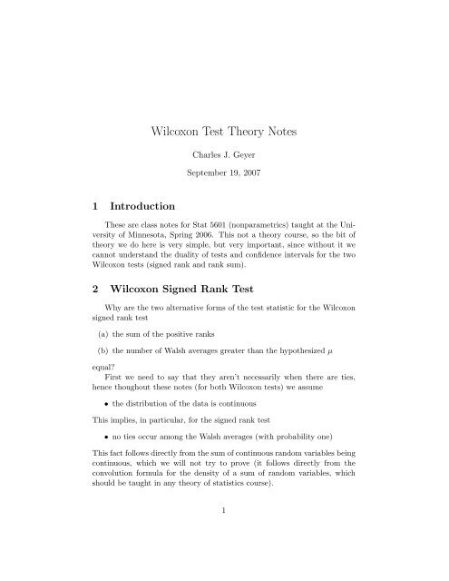
Wilcoxon Test Theory NotesCharles J. GeyerSeptember 19, 20071 IntroductionThese are class notes for Stat 5601 (nonparametrics) taught at the Universityof Minnesota, Spring 2006. This not a theory course, so the bit oftheory we do here is very simple, but very important, since without it wecannot understand the duality of tests and confidence intervals for the twoWilcoxon tests (signed rank and rank sum).2 Wilcoxon Signed Rank TestWhy are the two alternative forms of the test statistic for the Wilcoxonsigned rank test(a) the sum of the positive ranks(b) the number of Walsh averages greater than the hypothesized µequal?First we need to say that they aren’t necessarily when there are ties,hence thoughout these notes (for both Wilcoxon tests) we assume• the distribution of the data is continuousThis implies, in particular, for the signed rank test• no ties occur among the Walsh averages (with probability one)This fact follows directly from the sum of continuous random variables beingcontinuous, which we will not try to prove (it follows directly from theconvolution formula for the density of a sum of random variables, whichshould be taught in any theory of statistics course).1

So what this section will prove is that, assuming no ties among the Walshaverages, the two forms (a) and (b) are equal.The way proofs like this go is by mathematical induction. First we showthey are equal for some simple case. Then we show that any change to thedata keeps them equal. Hence we conclude they are equal no matter whatthe data are (as long as there are no ties).2.1 Base of the InductionThe simple case we start with is when the hypothesized value of theparameter of interest (population center of symmetry µ) is greater than alldata points, hence greater than all Walsh averages.Then if Z i are the data, all of the Z i − µ are negative hence all of theranks are negative and the sum of the positive ranks is zero.Similarly all of the Walsh averagesZ i + Z j, i ≤ j (1)2are less than µ, hence (b) is zero too.That finishes the start of the induction. We know (a) and (b) are equalfor this case (all of the data points below the hypothesized µ).2.2 Induction StepsNow we consider moving µ keeping the data fixed from past the upperend of the data (where we now know the values of the alternative formsof the test statistic) to past the lower end of the data, where symmetryconsiderations tell us both forms take on their maximal value n(n + 1)/2.Clearly, (b) changes value when and only when µ moves past a Walshaverage.Changes of value of (a) are more complicated. It changes value when• the ranks of some of the |Z i − µ| change, or• the signs attached to some of the ranks change.Latter first. Clearly the sign of Z i − µ changes when µ moves past Z i ,which is a Walsh average, the case i = j in (1).The rank of |Z i − µ| cannot change by itself. Some other rank, say thatof |Z j − µ| must change too. If we are looking at a very small change inµ causing the change, as these move past each other, they must be equal.2

Furthermore they cannot have the same sign, because decreasing µ cannotchange the order of Z i − µ and Z j − µ. Thus when they are equal we musthave(Z i − µ) = −(Z j − µ) (2)which implies µ = (Z i + Z j )/2. Hence in this case too, (a) changes when µmoves past a Walsh average.To summarize this section, we have proved: (a) and (b) change onlywhen µ moves past a Walsh average (of one kind or the other).2.2.1 Induction Step at a Data PointWhen i = j in (1), then the Walsh average is just Z i . In this section weconsider what happens when µ moves past Z i (going from right to left onthe number line)Clearly, (b) is increased by one. There is exactly one Walsh averageequal to Z i and when µ moves past that, there is one more Walsh averagegreater than µ.Clearly, (a) is also increased by one. Exactly one signed rank changes,that associated with Z i , when µ moves past Z i . When µ is very near Z i , inwhich case |Z i − µ| is the smallest of all the |Z j − µ|, hence the i-th rank isone, and the sign is negative when µ > Z i and positive when µ < Z i .2.2.2 Induction Step at other Walsh AveragesThe word “other” in the heading means those not yet considered. Supposei ≠ j and consider what happens when µ moves past the Walsh averagew = (Z i + Z j )/2 (going from right to left on the number line). As µ movespast w, at some point it is equal to w, and µ = w implies (2).Since Z i and Z j are not tied, we must have one greater and one less thanw, say (without loss of generality) Z i < w < Z j .For µ just a little above w we have the i-th rank greater than the j-thand for for µ just a little below w we have the i-th rank less than the j-th.Moreover the i-th is a negative rank (because Z i − µ is negative) and thej-th is a positive rank (because Z j − µ is positive). Finally the i-th andj-th absolute ranks are consecutive integers because as |Z i − µ| and |Z j − µ|change places in the rank order there is no room between them for otherZ m − µ. Thus as µ passes w going from right to left the j-th rank (whichis positive) increases by one, the i-th rank decreases by one (but is negativeand does not count), and none of the other ranks or signs change. Hencethe form (a) increases by one.3

And that finishes the proof. In all cases, no matter where µ is, (a) and(b) change in sync and hence are equal no matter where µ is.3 Wilcoxon Rank Sum TestThe situation for the rank sum test is similar. There are two alternativetest statistics, which, although not identical, differ only by a constant. Ifthe data are X 1 , . . ., X m and Y 1 , . . ., Y n and the hypothesized value of theshift is µ, meaning that under the null hypothesis we assume that the X iand the Y j − µ have the same distribution, then the test statistics are(a) the sum of the y ranks(b) the number of Y j − X i differences greater than the hypothesized µ.The former (a) we call the Wilcoxon statistic W . The latter (b) we call theMann-Whitney statistic U. To be more precise, to calculate W we assignranks to the m + n numbers of the form X i and Y j − µ and W is the sum ofthe ranks of the Y j − µ.In this section we prove two things.• W and U differ by a constant, which we identify.• The distributions W and U are symmetric about the midpoints of theirranges, which we also identify.As with the theory for the signed rank test, the proof of the first proceedsby induction. Throughout we assume no ties in the data.3.1 Base of the InductionThe proof by induction moves the hypothesized value µ from right to leftalong the number line (this is just like the proof for the signed rank test).As µ decreases, all of the Y j − µ values increase in synchrony, moving frombelow all the X i values (when µ is very large and positive) to above all theX i values (when µ is very large and negative).When µ is very large and positive, so all of the Y j − µ are to the left ofall the X i , U is zero (all of the Y j − X i are less than µ) and the Y ranks arethe numbers from 1 to n, so W = n(n + 1)/2 andW = U +n(n + 1). (3)24

3.1.1 Induction StepWe now need to show that as µ moves from left to right along the numberline U and W change in synchrony. Clearly W changes whenever some Y j −µis equal to some X j . Clearly U changes whenever some Y j − X i is equal toµ. Clearly both of these are the same event. WriteZ ij = Y j − X i .As µ moves from just above to just below Z ij the ranks assigned to X i andY j − µ swap. The one for X j decreasing by one and the one for Y j − µincreasing by one, so W increases by one. As µ moves from just above tojust below Z ij the number of Z ij greater than µ increases by one, so Uincreases by one.And that concludes the proof; (3) always holds.3.2 SymmetrySymmetry is easier to see for the Mann-Whitney test statistic. The wayto make it easy is to envisage the X’s to be sampled before the Y ’s and toenvisage the Y ’s arriving one at a time. So consider m X’s and one Y (takethe null hypothesis to be zero, so Y j − µ is just Y j ).Under the null hypothesis, these m + 1 variables are IID, hence the Y isequally probable to be any place in the sorted order; from 1 to m + 1. Thusthe number of Y j − X i pairs that exceed µ = 0 ranges from 0 to m and eachof these m + 1 numbers is equally probable. In short the contribution to Ufrom all the X’s and one Y has the discrete uniform distribution on the set{0, . . . , m}. Since the contributions of the Y ’s are IID (the Y ’s being IIDand independent of the X’s), we see that U is the sum of n IID discreteuniform {0, . . . , m} random variables.We take as a fact from theory (not difficult to prove) that the IID sum ofsymmetric random variables is symmetric. The discrete uniform distributionis symmetric, thus the distribution of U is symmetric. This discrete uniformdistribution has center of symmetry m/2, which is also the mean. The meanof the sum of n IID random variable is n times the mean of one of them,thusE(U) = mn2and this is also the center of symmetry and the median of the distributionof U. The range of U is from 0 to mn, which also makes it obvious the thecenter of symmetry, which must be the midpoint of the range, is mn/2.5

From (3) we know thatE(W ) = E(U) +n(n + 1)2=n(m + n + 1)2and this is also the center of symmetry and the median of the distributionof W . The range of W is found by adding n(n + 1)/2 to the range of U,giving lower endn(n + 1)2and upper endmn +n(n + 1)2=n(2m + n + 1)26