ruling out possible secondary stars to exoplanet host stars using the ...

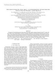
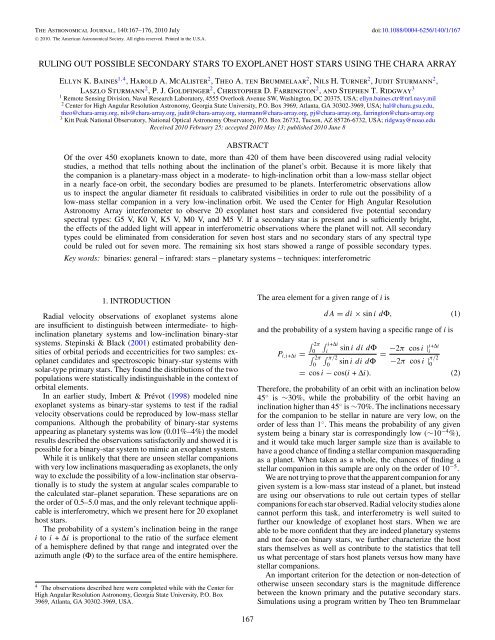
The Astronomical Journal, 140:167–176, 2010 JulyC○ 2010. The American Astronomical Society. All rights reserved. Printed in the U.S.A.doi:10.1088/0004-6256/140/1/167RULING OUT POSSIBLE SECONDARY STARS TO EXOPLANET HOST STARS USING THE CHARA ARRAYEllyn K. Baines 1,4 , Harold A. McAlister 2 , Theo A. ten Brummelaar 2 , Nils H. Turner 2 , Judit Sturmann 2 ,Laszlo Sturmann 2 , P. J. Goldfinger 2 , Christopher D. Farrington 2 , and Stephen T. Ridgway 31 Remote Sensing Division, Naval Research Laboratory, 4555 Overlook Avenue SW, Washington, DC 20375, USA; ellyn.baines.ctr@nrl.navy.mil2 Center for High Angular Resolution Astronomy, Georgia State University, P.O. Box 3969, Atlanta, GA 30302-3969, USA; hal@chara.gsu.edu,theo@chara-array.org, nils@chara-array.org, judit@chara-array.org, sturmann@chara-array.org, pj@chara-array.org, farrington@chara-array.org3 Kitt Peak National Observatory, National Optical Astronomy Observatory, P.O. Box 26732, Tucson, AZ 85726-6732, USA; ridgway@noao.eduReceived 2010 February 25; accepted 2010 May 13; published 2010 June 8ABSTRACTOf the over 450 exoplanets known to date, more than 420 of them have been discovered using radial velocitystudies, a method that tells nothing about the inclination of the planet’s orbit. Because it is more likely thatthe companion is a planetary-mass object in a moderate- to high-inclination orbit than a low-mass stellar objectin a nearly face-on orbit, the secondary bodies are presumed to be planets. Interferometric observations allowus to inspect the angular diameter fit residuals to calibrated visibilities in order to rule out the possibility of alow-mass stellar companion in a very low-inclination orbit. We used the Center for High Angular ResolutionAstronomy Array interferometer to observe 20 exoplanet host stars and considered five potential secondaryspectral types: G5 V, K0 V, K5 V, M0 V, and M5 V. If a secondary star is present and is sufficiently bright,the effects of the added light will appear in interferometric observations where the planet will not. All secondarytypes could be eliminated from consideration for seven host stars and no secondary stars of any spectral typecould be ruled out for seven more. The remaining six host stars showed a range of possible secondary types.Key words: binaries: general – infrared: stars – planetary systems – techniques: interferometric1. INTRODUCTIONRadial velocity observations of exoplanet systems aloneare insufficient to distinguish between intermediate- to highinclinationplanetary systems and low-inclination binary-starsystems. Stepinski & Black (2001) estimated probability densitiesof orbital periods and eccentricities for two samples: exoplanetcandidates and spectroscopic binary-star systems withsolar-type primary stars. They found the distributions of the twopopulations were statistically indistinguishable in the context oforbital elements.In an earlier study, Imbert & Prévot (1998) modeled nineexoplanet systems as binary-star systems to test if the radialvelocity observations could be reproduced by low-mass stellarcompanions. Although the probability of binary-star systemsappearing as planetary systems was low (0.01%–4%) the modelresults described the observations satisfactorily and showed it ispossible for a binary-star system to mimic an exoplanet system.While it is unlikely that there are unseen stellar companionswith very low inclinations masquerading as exoplanets, the onlyway to exclude the possibility of a low-inclination star observationallyis to study the system at angular scales comparable tothe calculated star–planet separation. These separations are onthe order of 0.5–5.0 mas, and the only relevant technique applicableis interferometry, which we present here for 20 exoplanethost stars.The probability of a system’s inclination being in the rangei to i + Δi is proportional to the ratio of the surface elementof a hemisphere defined by that range and integrated over theazimuth angle (Φ) to the surface area of the entire hemisphere.4 The observations described here were completed while with the Center forHigh Angular Resolution Astronomy, Georgia State University, P.O. Box3969, Atlanta, GA 30302-3969, USA.The area element for a given range of i isdA = di × sin idΦ, (1)and the probability of a system having a specific range of i is∫ 2π ∫ i+Δi0 i∫ 2π ∫ π/20sin ididΦ −2π cos i |i+ΔiiP i,i+Δi ==0sin ididΦ −2π cos i | π/20= cos i − cos(i + Δi). (2)Therefore, the probability of an orbit with an inclination below45 ◦ is ∼30%, while the probability of the orbit having aninclination higher than 45 ◦ is ∼70%. The inclinations necessaryfor the companion to be stellar in nature are very low, on theorder of less than 1 ◦ . This means the probability of any givensystem being a binary star is correspondingly low (∼10 −4 %),and it would take much larger sample size than is available tohave a good chance of finding a stellar companion masqueradingas a planet. When taken as a whole, the chances of finding astellar companion in this sample are only on the order of 10 −5 .We are not trying to prove that the apparent companion for anygiven system is a low-mass star instead of a planet, but insteadare using our observations to rule out certain types of stellarcompanions for each star observed. Radial velocity studies alonecannot perform this task, and interferometry is well suited tofurther our knowledge of exoplanet host stars. When we areable to be more confident that they are indeed planetary systemsand not face-on binary stars, we further characterize the hoststars themselves as well as contribute to the statistics that tellus what percentage of stars host planets versus how many havestellar companions.An important criterion for the detection or non-detection ofotherwise unseen secondary stars is the magnitude differencebetween the known primary and the putative secondary stars.Simulations using a program written by Theo ten Brummelaar167

168 BAINES ET AL. Vol. 140that realistically models instrumental and atmospheric noises,as well as observations of pairs of known brightness contrasts,indicate that the Array is sensitive to a magnitude difference inthe K band (ΔK) of 3.0. Therefore, if a second star is presentand is not more than ∼3.0 mag fainter than the host star, theeffects of the second star will be seen in the interferometric data.It should be noted that a limiting magnitude difference in the Kband (ΔK) of 3.0 is a lower limit, as the true ΔK also dependson the absolute brightness of the two stars and could be slightlyhigher for some systems.This technique of using interferometric observations to eliminatethe possibility of certain types of secondary stars was employedto examine the exoplanet host star 51 Peg (HD 217014)by Boden et al. (1998), whose analysis of Palomar Testbed Interferometerdata supported a single-star model for that star. Theyfit single-star and binary-star models to the data and found thatany possible unseen stellar companion would have to have aK-magnitude fainter than 7.30 and a mass of less than 0.22 M ⊙ .Here, we describe our interferometric observations, ourmethod for choosing calibrator stars, and define the role interferometricresolution plays in Section 2. In Section 3, wediscuss how the angular diameter fit residuals to calibrated visibilitiescan help us eliminate certain types of secondary stars;and Section 4 explores the implications of the observations. Thispaper is follow-on work to an earlier study (Baines et al. 2008b).2. INTERFEROMETRIC OBSERVATIONSAll observations were obtained using the Center for HighAngular Resolution Astronomy (CHARA) Array, a six-elementoptical/infrared interferometric array located on Mount Wilson,CA (ten Brummelaar et al. 2005). We used the pupil-plane“CHARA Classic” beam combiner in the K ′ band (2.133 μmcenter with a 0.349 μm width), while visible wavelengths(470–800 nm) were used for tracking and tip/tilt corrections.The observing procedure and data reduction process employedhere are described in McAlister et al. (2005). The observablequantity from an interferometer is the fringe contrast or “visibility”of the observed target, and each data set consists ofapproximately 200 scans across the fringe.Our target list was selected from the complete exoplanet listby using declination limits and magnitude constraints: north of−10 ◦ declination, brighter than V = +10 in order for the tip/tilt system to lock onto the star, and brighter than K = +6.5for reliable fringe detection with a sufficiently high signal-tonoiseratio. We obtained data on the 20 exoplanet host starsbetween 2005 October and 2008 September. The observationswere taken using mostly the longest baseline available on theCHARA Array (331 m), though 156 m and 249 m baselineswere also used.Reliable calibrators stars are critical in interferometric observations,acting as the standard against which the sciencetarget is measured, and the ideal calibrator is a single, spherical,non-variable star. Our observing pattern was calibrator-targetcalibratorso that every target was bracketed by calibrator observationsmade as close in time as possible; therefore, “fivebracketed observations” denote five target and six calibratordata sets. The target–calibrator (T–C) distances ranged from 1 ◦to 9 ◦ and 13 calibrators were within 4 ◦ of their target stars.This allowed us to observe the stars as close together in timeas possible, usually on the order of 3–5 minutes between thetwo, therefore, reducing the effects of changing seeing conditionsas much as possible. Table 1 lists the exoplanet host starsobserved, their calibrators, the dates of the observations, theTable 1Observing LogTarget Calibrator Baseline Date No. T–C SepHD HD (max. length) (UT) Obs (deg)10697 10477 S1–E1 (331 m) 2005 Oct 23 4 42007 Sep 14 413189 11007 S1–E1 (331 m) 2005 Dec 12 4 42006 Aug 14 432518 31675 S1–E1 (331 m) 2007 Nov 14 9 345410 46590 S1–E1 (331 m) 2008 Sep 11 5 250554 49736 S1–E1 (331 m) 2005 Dec 12 5 273108 69548 E2–W2 (156 m) 2008 May 9 5 7136726 145454 E2–W2 (156 m) 2008 May 9 6 6139357 132254 S1–E1 (331 m) 2007 Sep 14 4 7145675 151044 S1–E1 (331 m) 2006 Aug 12 6 8154345 151044 S1–E1 (331 m) 2008 Sep 10 7 4164922 159139 S1–E1 (331 m) 2008 Aug 11 5 7167042 161693 S1–E1 (331 m) 2007 Sep 15 8 4170693 172569 W1–S2 (249 m) 2007 Sep 3 4 1185269 184381 S1–E1 (331 m) 2008 Jul 18 15 32008 Jul 20 5188310 182101 S1–E1 (331 m) 2008 Sep 8 8 8199665 194012 S1–E1 (331 m) 2008 Sep 8 10 9210702 210074 S1–E1 (331 m) 2008 Sep 8 4 4217107 217131 S1–E1 (331 m) 2008 Sep 8 5 1221345 222451 S1–E1 (331 m) 2008 Sep 11 5 3222404 219485 S1–E1 (331 m) 2008 Sep 11 7 4Notes. The three arms of the Array are denoted by their cardinal directions: “S”is south, “E” is east, and “W” is west. Each arm bears two telescopes, numbered“1” for the telescope farthest from the beam combining laboratory and “2” forthe telescope closer to the lab.baseline used, the number of observations obtained, and theT–C distance.In order to check for excess emission that could indicate a lowmassstellar companion or circumstellar disk, we fitted spectralenergy distributions (SEDs) based on published UBVRIJHKphotometric values for each calibrator star. Limb-darkeneddiameters were calculated using Kurucz model atmospheres 5based on effective temperature and gravity values obtained fromthe literature. The models were then fit to observed photometricvalues also from the literature after converting magnitudes tofluxes using Colina et al. (1996) forUBVRI values and Cohenet al. (2003) forJHK values.Many of the calibrator stars chosen here had been used ascomparison or calibrator stars in other studies, or speckle studiesdid not find companions (see Table 2). For those calibrator starsthat had not been previously observed, their SED fits showed noexcess flux that could indicate a stellar companion that wouldthen contaminate our interferometric observations.Our ability to detect stellar companions depends on two mainfactors. The first is the precision of our visibility measurements.The higher the precision, the higher our sensitivity to findinga secondary companion. The second factor is whether themeasured angular diameters or potential primary–secondaryseparation would be resolved in our data. The resolution of aninterferometer depends on the wavelength used and the distancebetween the telescopes, otherwise known as the baseline. A staris considered unresolved if its visibility is ∼ =1 and is completelyresolved when its visibilities drop to zero. Differently sized starswill be resolved at different baselines (see Figure 1).5 See http://kurucz.cfa.harvard.edu.

No. 1, 2010 EXOPLANET HOST STAR COMPANIONS 169Figure 1. Effect of various stellar angular diameters on the visibility curve. The smaller a star’s angular diameter, the less change is seen in the visibility curve as afunction of baseline.Table 2Notes on Calibrator Quality and Previous UsesHDDetails10477 No sign of duplicity in literature or SED fit11007 Listed as a “suitable” calibrator in van Belle et al. (2008);used as calibrator in Konacki & Lane (2004)31675 No companion found using speckle in McAlister et al. (1989)46590 No sign of duplicity in literature or SED fit49736 No sign of duplicity in literature or SED fit69548 No sign of duplicity in literature or SED fit132254 Listed as a “probably suitable” calibrator in van Belle et al. (2008);no companion found using speckle in McAlister et al. (1989)145454 No sign of duplicity in literature or SED fit151044 Listed as a “probably suitable” calibrator in van Belle et al. (2008)159139 No companion found using speckle in McAlister et al. (1987)161693 No companion found using speckle in McAlister et al. (1987)172569 Listed in “HIP Visual Binaries Kinematics” table by Bartkevicius & Gudas (2001);but no other information given in paper or general literature182101 Used as calibrator in Berger et al. (2006)184381 Used as comparison star in Johnson et al. (2006)194012 Listed as a “suitable” calibrator in van Belle et al. (2008);no companion found using speckle in McAlister et al. (1987)210074 Listed as a “suitable” calibrator in van Belle et al. (2008);used as comparison star in Wittenmyer et al. (2005)217131 No companion found using speckle in McAlister et al. (1987)219485 No sign of duplicity in literature or SED fit222451 No sign of duplicity in literature or SED fitAnother effect to account for is bandwidth smearing, whichoccurs when the physical width of the filter’s bandpass affectsthe measurements as the resolution varies across the band.Bandwidth smearing is only significant when a star’s angulardiameter exceeds the coherent field of view of the interferometer,which is calculated to beFOV = θ minπ( Δλλ 0) −1, (3)

170 BAINES ET AL. Vol. 140Table 3Exoplanet Host Stars’ Calibrated VisibilitiesTarget MJD B Θ V c σV c %Name (m) (deg) Error10697 53666.427 309.50 175.2 1.043 0.090 953666.443 310.79 171.2 0.928 0.068 753666.456 312.37 167.9 1.004 0.104 1053666.470 314.46 164.6 0.832 0.075 954356.765 317.17 226.9 0.883 0.103 1254356.775 320.54 227.4 1.029 0.125 1254357.783 323.64 228.1 0.851 0.077 954357.792 325.84 228.8 0.723 0.068 954357.802 327.87 229.7 0.816 0.089 1154357.810 328.95 230.4 0.791 0.061 813189 53716.270 327.09 184.4 0.607 0.056 953716.285 326.91 180.9 0.531 0.081 1553716.298 326.96 177.7 0.589 0.095 1653716.312 327.21 174.3 0.575 0.130 2353961.441 326.60 216.4 0.622 0.051 853961.454 328.41 214.4 0.648 0.062 1053961.467 329.65 212.2 0.643 0.073 1153961.481 330.38 209.8 0.607 0.040 732518 54418.238 230.84 200.1 0.755 0.067 954418.244 233.56 201.8 0.794 0.071 954418.250 236.48 203.6 0.834 0.070 854418.256 239.18 205.3 0.843 0.074 954418.261 241.66 206.9 0.751 0.061 854418.267 244.20 208.6 0.743 0.053 754418.274 246.86 210.3 0.776 0.059 854418.280 249.36 212.0 0.741 0.065 954418.286 251.81 213.8 0.732 0.053 745410 54720.481 258.11 212.9 0.696 0.078 1154720.490 263.24 215.0 0.651 0.053 854720.496 266.69 216.4 0.587 0.073 1254720.502 269.68 217.7 0.665 0.106 1654720.509 272.90 219.2 0.716 0.097 1450554 53711.523 317.33 174.2 0.874 0.127 1553711.537 318.32 170.7 0.783 0.090 1153716.422 321.04 195.4 1.006 0.138 1453716.435 319.48 192.2 0.905 0.091 1053716.449 318.20 189.0 0.984 0.083 853716.463 317.30 185.7 1.027 0.096 953716.479 316.73 181.7 0.956 0.150 1673108 54595.216 155.95 254.7 0.411 0.051 1254595.226 155.88 258.0 0.446 0.034 854595.235 155.83 261.1 0.436 0.043 1054595.244 155.80 264.1 0.460 0.057 1254595.257 155.77 268.4 0.430 0.092 21136726 54595.294 147.57 189.4 0.442 0.055 1254595.307 148.79 193.7 0.425 0.045 1154595.315 149.53 196.5 0.468 0.054 1254595.325 150.30 199.6 0.421 0.056 1354595.336 151.17 203.4 0.436 0.062 1454595.346 151.80 206.5 0.409 0.053 13139357 54357.149 320.57 102.8 0.450 0.070 1654357.155 320.14 104.2 0.460 0.045 1054357.161 319.66 105.6 0.487 0.063 1354357.167 319.12 107.1 0.491 0.066 1354358.151 320.24 103.9 0.460 0.030 754358.157 319.77 105.3 0.415 0.034 854358.162 319.27 106.7 0.429 0.049 11145675 53958.259 329.81 168.4 0.902 0.054 653958.275 329.38 164.9 0.878 0.045 553958.292 328.62 161.0 0.859 0.051 653959.168 329.99 189.3 1.096 0.123 1153959.184 330.18 185.5 1.000 0.089 953959.200 330.26 181.8 0.964 0.069 753959.215 330.26 178.1 0.990 0.070 753959.231 330.18 174.5 0.940 0.078 8Table 3(Continued)Target MJD B Θ V c σV c %Name (m) (deg) Error53959.246 330.01 170.9 0.954 0.067 753959.261 329.70 167.4 0.808 0.064 8154345 54719.168 328.79 90.5 0.885 0.094 1154719.179 328.73 93.3 0.843 0.109 1354719.185 328.66 94.7 0.811 0.089 1154719.192 328.57 96.2 0.803 0.096 1254719.198 328.45 97.6 0.847 0.096 1154719.204 328.29 99.2 0.903 0.095 1154719.213 328.00 101.4 0.817 0.122 15164922 54689.201 326.49 248.8 0.663 0.089 1354689.212 325.27 251.2 0.820 0.058 754689.223 324.07 253.6 0.957 0.079 854689.235 322.84 256.4 1.067 0.153 1454689.248 321.74 259.4 1.011 0.170 17167042 54358.232 321.20 97.5 0.584 0.037 654358.238 320.96 99.0 0.551 0.036 754358.243 320.68 100.3 0.507 0.036 754358.249 320.34 101.7 0.524 0.030 654358.255 319.96 103.1 0.571 0.036 654358.261 319.53 104.5 0.612 0.037 654358.267 319.05 105.9 0.591 0.041 754358.273 318.48 107.4 0.627 0.050 8170693 54346.303 187.40 183.8 0.373 0.042 1154346.311 183.87 186.6 0.343 0.049 1454346.321 179.32 190.2 0.358 0.037 1054346.332 174.70 193.9 0.457 0.042 9185269 54665.204 321.00 228.6 0.860 0.146 1754665.216 323.97 230.0 0.946 0.129 1454665.226 326.17 231.3 0.757 0.148 2054665.236 327.81 232.6 0.926 0.110 1254665.245 328.96 233.9 0.928 0.178 1954665.404 323.06 266.1 0.771 0.064 854665.410 322.92 267.7 0.741 0.050 754665.417 322.85 269.2 0.816 0.048 654665.423 322.85 90.8 0.921 0.057 654665.430 322.93 92.4 0.877 0.075 954665.438 323.11 94.3 0.912 0.084 954665.445 323.35 96.0 0.910 0.091 1054665.452 323.68 97.7 0.855 0.080 954665.459 324.06 99.4 0.927 0.083 954665.466 324.52 101.1 0.841 0.129 1554667.381 323.73 262.0 1.004 0.096 1054667.387 323.44 263.5 0.830 0.103 1254667.393 323.21 264.9 0.892 0.096 1154667.400 323.02 266.5 1.014 0.085 854667.406 322.90 267.9 0.899 0.113 13188310 54717.211 293.54 249.5 0.103 0.014 1454717.223 289.87 252.2 0.106 0.017 1654717.229 288.10 253.7 0.107 0.012 1154717.236 286.11 255.5 0.106 0.014 1354717.242 284.72 257.0 0.094 0.015 1654717.248 283.37 258.5 0.110 0.019 1754717.253 282.29 260.0 0.111 0.018 1654717.259 281.25 261.6 0.127 0.018 14199665 54717.336 285.96 90.6 0.614 0.064 1054717.341 286.09 92.1 0.567 0.062 1154717.347 286.36 93.6 0.562 0.077 1454717.352 286.78 95.0 0.574 0.053 954717.358 287.37 96.6 0.566 0.060 1154717.364 288.15 98.2 0.512 0.055 1154717.370 289.11 99.1 0.479 0.069 1454717.377 290.31 101.5 0.482 0.049 1054717.383 291.58 103.1 0.414 0.035 854717.390 293.30 104.9 0.500 0.065 13210702 54717.426 302.96 100.6 0.635 0.076 12

No. 1, 2010 EXOPLANET HOST STAR COMPANIONS 171Table 3(Continued)Target MJD B Θ V c σV c %Name (m) (deg) Error54717.436 304.66 103.1 0.652 0.072 1154717.442 305.68 104.5 0.591 0.085 1454717.448 306.87 105.9 0.640 0.091 14217107 54717.283 292.41 236.3 0.771 0.096 1254717.289 289.09 237.2 0.793 0.127 1654717.296 285.35 238.3 0.757 0.095 1354717.303 281.40 239.5 0.799 0.118 1554717.309 278.11 240.6 0.776 0.114 15221345 54720.234 313.74 229.1 0.278 0.031 1154720.239 315.41 229.9 0.253 0.034 1354720.245 317.13 230.8 0.266 0.028 1154720.250 318.64 231.7 0.232 0.024 1054720.256 320.12 232.7 0.251 0.028 11222404 54664.457 253.07 230.4 0.105 0.011 1054664.466 254.63 233.0 0.099 0.011 1154664.475 256.07 235.6 0.091 0.010 1154720.278 247.87 222.5 0.104 0.012 1254720.285 249.26 224.5 0.093 0.010 1154720.295 251.32 227.6 0.093 0.008 954720.301 252.45 229.3 0.086 0.008 954720.307 253.58 231.2 0.092 0.009 1054720.313 254.70 233.2 0.091 0.008 954720.320 255.83 235.2 0.087 0.009 10Note. The projected baseline position angle (Θ) is calculated to be east of north.where θ min = λ 0 /B and B is the baseline, λ 0 is the centralwavelength of the filter, and Δλ is the width of the filter (Tango&Davis2002). Because our coherent FOV is larger than themeasured angular diameters in all cases, we do not need tocorrect for this effect when measuring our primary exoplanethost stars. On the other hand, when we determine the visibilitiesfor binary systems that have calculated separations larger thanthe FOV, we need to account for bandwidth smearing by usinga modified version of the visibility equation for binary stars.3. CHARACTERIZING ANGULAR DIAMETER FITRESIDUALS TO CALIBRATED VISIBILITIESTo determine stellar angular diameters, measured visibilities(V) are fit to a model of a uniformly illuminated disk (UD).Single-star diameter fits to V were based upon the UD approximationgiven by V = [2J 1 (x)]/x, where J 1 is the first-orderBessel function and x = πBθ UD λ −1 , where B is the projectedbaseline at the star’s position, θ UD is the apparent UD angulardiameter of the star, and λ is the effective wavelength of theobservation (Shao & Colavita 1992). A more realistic modelof a star’s disk involves limb-darkening (LD), and the relationshipincorporating the linear limb-darkening coefficient μ λ(Hanbury-Brown et al. 1974) isV =(1 − μ λ2(π+ μ λ2) −1×[+ μ λ3) 1/2 ]J3/2 (x). (4)x 3/2(1 − μ λ ) J 1(x)xTable 3 lists the Modified Julian Date (MJD), baseline B,projected baseline position angle (Θ), calibrated visibility (V c ),and error in V c (σV c ) for each star observed, and the resultingangular diameters are presented in Table 4. Figure 2 showsthe LD diameter fit for HD 164922 as this star’s diameter ispresented for the first time here. Similar plots for the remainingstars can be found in the references listed in Table 4.The systematics in the residuals of the angular diameter fitto measured visibilities can help us eliminate certain types ofpotential secondary stars. The smaller the residuals, the lowerthe chance of an unseen stellar companion. For each exoplanethost star observed, a variety of secondary stars were considered:G5 V, K0 V, K5 V, M0 V, and M5 V. The magnitude difference(ΔM K , listed as ΔK in the tables) and angular separation (α)of a face-on orbit between the host star and companion werecalculated for each possible pairing:ΔM K = M s +(m h − M h ) − m h , (5)where M h,s are the absolute magnitudes of the host star andpotential secondary, respectively, m h is the apparent magnitudeof the host star, and( ) 100(m h − M h ) = 5log , (6)πwhere π is the host star’s parallax in milliarcsecond (mas). Anestimate of the angular separation α in mas was calculated fromKepler’s third law:α = [(M h + M s ) × P 2 ] 1 3 × π, (7)where M h,s are the masses in M ⊙ of the exoplanet’s host star andpotential secondary star, respectively, and P is the companion’sorbital period in years.The angular diameter (θ) for each possible secondary starwas estimated using the calibration of radius as a function ofspectral type from Cox (2000) and the parallax of the hoststar. The masses and radii in Cox are based on values derivedfrom Habets & Heintze (1981), who observed binary stars inorder to create empirical relationships between various stellarparameters as a function of luminosity class. Tables 4 and 5present the results of these calculations.The resulting values for θ, ΔK, and α were then used todetermine the visibility curve for a single star with the hoststar’s measured angular diameter as well as for a binary systemwith the parameters listed above. The equation used to calculatethe visibility curve for a binary system when observed using anarrow bandpass isV = (1 + β) −1[ V 21 + β2 V 22 +2βV 1V 2 cos{2πBλ −1 α cos φ} ] 1 2,(8)where V 1,2 are the visibilities for the primary and secondarystar, respectively, β = 100 0.2Δm , where Δm is the magnitudedifference between the two stars, and φ is the difference of theposition angles between the binary and the baseline (HanburyBrown et al. 1970). Because the observations described herewere taken using a filter with a bandpass of ∼16%, the equationneeds to be modified to include the effects of wide bandwidthand bandwidth smearing (North et al. 2007):V = (1 + β) −1[ V 21 + β2 V 22 +2βr(ψ)V 1V 2 cos ψ ] 1 2, (9)where ψ = 2πBλ −1 α cos φ and( −Δλ2ψ 2 )r(ψ) = exp. (10)32 ln 2λ 2 0

172 BAINES ET AL. Vol. 140Figure 2. HD 164922 LD disk diameter fit. The solid line represents the theoretical visibility curve for the star with the best-fit θ LD , the dashed lines are the 1σ errorlimits of the diameter fit, the squares are the calibrated visibilities, and the vertical lines are the measured errors.Table 4Exoplanet Host Star and Planet Observed ParametersHD Observed Stellar Parameters Planetary System Parameters (m − M)Spectral θ LD σ LD K π M star P ReferenceType (mas) (%) (mag) (mas) (M ⊙ ) (d)10697 G5 IV 0.49 ± 0.05 a 10 4.60 ± 0.02 30.70 ± 0.43 1.2 1076.4 Butler et al. (2006) 2.613189 K2 0.84 ± 0.03 a 4 4.00 ± 0.03 1.78 ± 0.73 3.5 b 472 P from Hatzes et al. (2005) 8.732518 K1 III 0.85 ± 0.02 c 2 3.91 ± 0.04 8.29 ± 0.58 1.1 157.5 Döllinger et al. (2009a) 5.445410 K0 III-IV 0.97 ± 0.04 d 4 3.70 ± 0.30 17.92 ± 0.47 1.7 889 Sato et al. (2008b) 3.750554 F8 V 0.34 ± 0.10 a 29 5.47 ± 0.02 33.43 ± 0.59 1.1 1254 Fischer et al. (2002) 2.473108 K1 III 2.23 ± 0.02 c 1 1.92 ± 0.07 12.74 ± 0.26 1.2 269.3 Döllinger et al. (2007) 4.5136726 K4 III 2.34 ± 0.02 c 1 1.92 ± 0.05 8.19 ± 0.19 1.8 516.2 Döllinger et al. (2009a) 5.4139357 K4 III 1.07 ± 0.01 c 1 3.41 ± 0.32 8.47 ± 0.30 1.3 1125.7 Döllinger et al. (2009b) 5.4145675 K0 V 0.37 ± 0.04 a 11 4.71 ± 0.02 56.91 ± 0.34 1.0 1724.0 Butler et al. (2003) 1.2154345 G8 V 0.50 ± 0.03 d 6 5.00 ± 0.02 53.80 ± 0.32 0.9 3360 Wright et al. (2008) 1.3164922 K0 V 0.50 ± 0.07 e 14 5.11 ± 0.02 45.21 ± 0.54 0.9 1155 Butler et al. (2006) 1.7167042 K1 III 0.92 ± 0.02 c 2 3.55 ± 0.24 19.91 ± 0.26 1.5 418 Sato et al. (2008b) 3.5170693 K1.5 III 2.04 ± 0.04 c 2 1.95 ± 0.05 10.36 ± 0.20 1.0 479.1 Döllinger et al. (2009b) 4.9185269 G0 IV 0.48 ± 0.03 d 6 5.26 ± 0.02 19.89 ± 0.56 1.3 6.8 Johnson et al. (2006) 3.5188310 G9 III 1.73 ± 0.01 d 1 2.17 ± 0.22 17.77 ± 0.29 2.2 137 Sato et al. (2008a) 3.8199665 G6 III 1.11 ± 0.03 d 3 3.37 ± 0.20 13.28 ± 0.31 2.2 993 Sato et al. (2008a) 4.4210702 K1 III 0.88 ± 0.02 d 2 3.98 ± 0.29 18.20 ± 0.39 1.9 341.1 Johnson et al. (2007) 3.7217107 G8 IV 0.70 ± 0.01 d 1 4.54 ± 0.02 50.36 ± 0.38 1.0 7.1 Fischer et al. (1999) 1.5221345 G8 III 1.34 ± 0.01 d 1 2.33 ± 0.24 12.63 ± 0.27 2.2 186 Sato et al. (2008b) 4.5222404 K1 IV 3.30 ± 0.03 d 1 1.04 ± 0.21 70.91 ± 0.40 1.6 906 Hatzes et al. (2003) 0.7Notes. Spectral types are from SIMBAD; parallaxes π are from van Leeuwen (2007); K magnitudes are from Cutri et al. (2003), except for HD 73108, HD 136726,and HD 170693, which are from Neugebauer & Leighton (1969); (m − M) was calculated using Equation (3).a Baines et al. (2008a).b Mass from Schuler et al. (2005), though they cannot constrain the mass to better than 2–6 M ⊙ .c Baines et al. (2010).d Baines et al. (2009).e Previously unpublished.To explore the effects of the projected position angle of a binarystarvector separation, we calculated the residuals using positionangles of 0 ◦ ,30 ◦ , and 60 ◦ (see Table 6).To estimate the detection sensitivity, the largest differencebetween the visibility curves for a single star and for a binarysystem with the parameters listed in Table 5 was calculated.This quantity, ΔV max , then represented the maximum deviationof the binary visibility curve from the single-star curve. Figure 3shows an example of this.Due to uncertainties in such input parameters as the hoststar’s mass, parallax, and the planet’s orbital period used inEquations (3) and (4), we did not believe a 1σ threshold would

No. 1, 2010 EXOPLANET HOST STAR COMPANIONS 173Figure 3. Example of the difference between the visibility curves for a single star and a binary system. The solid line indicates the curve for a single star with θ = 1.0mas, while the dashed line represents the curve for a binary system with the following parameters: θ primary = 1.0 mas, θ secondary = 0.5 mas, α = 10 mas, and ΔK =2.0. ΔV max is the maximum deviation between the two curves.Table 5Calculated Parameters for Secondary Stars of Various Spectral TypesHD G5 V K0 V K5 V M0 V M5 VΔK α θ ΔK α θ ΔK α θ ΔK α θ ΔK α θ(mag) (mas) (mas) (mag) (mas) (mas) (mag) (mas) (mas) (mag) (mas) (mas) (mag) (mas) (mas)10697 1.5 80.6 0.26 1.9 78.8 0.24 2.5 77.2 0.21 3.1 74.9 0.17 4.1 70.1 0.0813189 8.3 3.5 0.02 8.7 3.4 0.01 9.3 3.4 0.01 9.9 3.4 0.01 10.9 3.3 0.0032518 5.0 6.0 0.07 5.4 5.9 0.07 6.0 5.8 0.06 6.6 5.6 0.05 7.6 5.2 0.0245410 3.5 44.7 0.15 3.9 43.9 0.14 4.5 43.2 0.12 5.2 42.2 0.10 6.2 40.2 0.0550554 0.4 95.6 0.29 0.8 93.5 0.26 1.4 91.4 0.22 2.1 88.5 0.19 3.0 82.5 0.0873108 6.1 13.4 0.11 6.5 13.1 0.10 7.1 12.9 0.09 7.7 12.5 0.07 8.7 11.7 0.03136726 7.0 14.4 0.07 7.4 14.2 0.06 8.0 13.9 0.05 8.7 13.6 0.05 9.6 13.0 0.02139357 5.5 23.4 0.07 5.9 23.0 0.07 6.5 22.5 0.06 7.1 21.9 0.05 8.1 20.6 0.02145675 0.0 199.0 0.49 0.4 194.4 0.45 1.0 190.0 0.38 1.7 183.7 0.32 2.6 170.6 0.14154345 −0.2 287.3 0.46 0.2 280.3 0.43 0.8 273.4 0.36 1.5 263.6 0.30 2.5 243.1 0.14164922 0.1 119.8 0.39 0.5 116.9 0.36 1.1 114.2 0.30 1.8 110.2 0.25 2.7 102.0 0.11167042 3.5 29.2 0.17 3.9 28.7 0.16 4.5 28.2 0.13 5.1 27.5 0.11 6.1 26.0 0.05170693 6.5 15.4 0.09 6.9 15.0 0.08 7.5 14.7 0.07 8.1 14.2 0.06 9.1 13.2 0.03185269 1.7 1.8 0.17 2.1 1.8 0.16 2.7 1.7 0.13 3.4 1.7 0.11 4.4 1.6 0.05188310 5.1 13.5 0.15 5.5 13.3 0.14 6.1 13.1 0.12 6.7 12.9 0.10 7.7 12.4 0.04199665 4.5 37.8 0.11 4.9 37.3 0.11 5.5 36.8 0.09 6.2 36.1 0.07 7.1 34.7 0.03210702 3.2 24.4 0.16 3.6 24.0 0.14 4.2 23.7 0.12 4.9 23.2 0.10 5.8 22.1 0.05217107 0.5 4.5 0.43 0.9 4.4 0.40 1.5 4.3 0.34 2.1 4.1 0.28 3.1 3.8 0.13221345 5.7 11.8 0.11 6.1 11.6 0.10 6.7 11.4 0.08 7.3 11.2 0.07 8.3 10.8 0.03222404 3.2 176.6 0.61 3.6 173.5 0.56 4.2 170.5 0.48 4.9 166.4 0.40 5.8 158.1 0.18Notes. Values for M K (used to calculate ΔK), secondary stellar masses (used to calculate α), and secondary stellar radii (used to calculate θ) were obtained from Cox(2000): G5 V = 3.5, 0.92 M ⊙ ,0.92R ⊙ ;K0V= 3.9, 0.79 M ⊙ ,0.85R ⊙ ;K5V= 4.5, 0.67 M ⊙ ,0.72R ⊙ ;M0V= 5.2, 0.51 M ⊙ ,0.60R ⊙ ;M5V= 6.1, 0.21 M ⊙ ,0.27 R ⊙ .be a reliable diagnostic. Therefore, in order to rule out putativestellar companions, we selected a lower limit of 2σ res , where σ resis the standard deviation of the residuals to the diameter fit; i.e., ifΔV max 2σ res for a given secondary component, then particularspectral type can be eliminated as a possible stellar companion.If ΔV max < 2σ res , the effects of the companion would not beclearly seen in the visibility curve, and that spectral type cannotbe ruled out. For each exoplanet host star, Table 6 lists theobserved σ res and the predicted ΔV max for each secondary typeobserved, and Table 7 indicates which secondary spectral typescan be eliminated from consideration for each host star at eachposition angle.4. RESULTS AND DISCUSSIONThough the errors for the individual calibrated visibilitieslisted in Table 3 are on the order of 2%–20%, the errorsfor the angular diameter fits to these visibilities are on theorder of 1%–6% for most stars. This is because the calibratedvisibility errors are overestimated. This can be best illustrated

174 BAINES ET AL. Vol. 140Table 6Observed Diameter Fit Residuals and Calculated Binary Visibility ResidualsHD Obs Date σ res ΔV max , P.A. = 0 ◦ ΔV max , P.A. = 30 ◦ ΔV max , P.A. = 60 ◦G5V K0V K5V M0V M5V G5V K0V K5V M0V M5V G5V K0V K5V M0V M5V10697 2005 Oct 23 0.092 0.221 0.162 0.098 0.058 0.024 0.232 0.164 0.096 0.055 0.022 0.225 0.162 0.098 0.058 0.0242007 Sep 14 0.053 0.221 0.162 0.098 0.058 0.024 0.232 0.164 0.096 0.055 0.022 0.225 0.162 0.098 0.058 0.02413189 2005 Dec 12 0.033 0.001 0.000 0.000 0.000 0.000 0.001 0.000 0.000 0.000 0.000 0.001 0.000 0.000 0.000 0.0002006 Aug 14 0.019 0.001 0.000 0.000 0.000 0.000 0.001 0.000 0.000 0.000 0.000 0.001 0.000 0.000 0.000 0.00032518 2007 Nov 14 0.036 0.011 0.008 0.005 0.003 0.001 0.012 0.008 0.005 0.003 0.001 0.011 0.008 0.005 0.003 0.00145410 2008 Sep 11 0.052 0.047 0.033 0.019 0.010 0.004 0.046 0.032 0.019 0.010 0.004 0.047 0.033 0.019 0.010 0.00450554 2005 Dec 12 0.047 0.448 0.346 0.213 0.112 0.057 0.445 0.365 0.238 0.135 0.062 0.485 0.384 0.244 0.137 0.06173108 2008 May 9 0.018 0.200 0.201 0.202 0.202 0.202 0.201 0.201 0.201 0.202 0.202 0.199 0.201 0.202 0.202 0.202136726 2008 May 9 0.018 0.194 0.194 0.194 0.194 0.195 0.194 0.194 0.194 0.194 0.195 0.193 0.194 0.194 0.194 0.195139357 2007 Sep 14 0.019 0.008 0.005 0.003 0.002 0.001 0.008 0.005 0.003 0.002 0.001 0.008 0.005 0.003 0.002 0.001145675 2006 Aug 12 0.056 0.543 0.460 0.302 0.166 0.076 0.401 0.420 0.301 0.165 0.046 0.542 0.459 0.302 0.169 0.077154345 2008 Sep 10 0.039 0.256 0.336 0.282 0.186 0.094 0.493 0.529 0.391 0.233 0.099 0.272 0.361 0.328 0.211 0.094164922 2008 Aug 11 0.161 0.564 0.489 0.322 0.183 0.082 0.608 0.481 0.306 0.167 0.069 0.562 0.487 0.321 0.183 0.082167042 2007 Sep 15 0.040 0.045 0.032 0.019 0.011 0.004 0.046 0.032 0.019 0.011 0.004 0.046 0.032 0.018 0.011 0.004170693 2007 Sep 3 0.037 0.219 0.219 0.220 0.220 0.220 0.219 0.219 0.220 0.220 0.220 0.218 0.219 0.220 0.220 0.220185269 2008 Jul 18 0.078 0.193 0.139 0.086 0.047 0.019 0.203 0.146 0.087 0.047 0.018 0.137 0.098 0.058 0.032 0.0132008 Jul 20 0.079 0.193 0.139 0.086 0.047 0.019 0.203 0.146 0.087 0.047 0.018 0.137 0.098 0.058 0.032 0.013188310 2008 Sep 8 0.012 0.151 0.152 0.153 0.154 0.155 0.151 0.152 0.153 0.154 0.155 0.152 0.152 0.153 0.154 0.155199665 2008 Sep 8 0.054 0.020 0.014 0.008 0.004 0.002 0.020 0.014 0.008 0.004 0.002 0.020 0.014 0.008 0.004 0.002210702 2008 Sep 8 0.025 0.060 0.042 0.024 0.013 0.006 0.059 0.041 0.024 0.013 0.006 0.059 0.041 0.024 0.013 0.006217107 2008 Sep 8 0.017 0.496 0.376 0.239 0.148 0.061 0.499 0.374 0.234 0.140 0.059 0.454 0.339 0.213 0.131 0.058221345 2008 Sep 11 0.013 0.007 0.005 0.003 0.002 0.001 0.007 0.005 0.003 0.002 0.001 0.007 0.005 0.003 0.002 0.001222404 2008 Sep 11 0.006 0.182 0.187 0.192 0.196 0.198 0.182 0.187 0.192 0.196 0.198 0.182 0.187 0.192 0.196 0.198Note. P.A. is the position angle.Table 7Eliminating Certain Secondary StarsHD Obs Date P.A. = 0 ◦ P.A. = 30 ◦ P.A. = 60 ◦G5V K0V K5V M0V M5V G5V K0V K5V M0V M5V G5V K0V K5V M0V M5V10697 2005 Oct 23 X P P P P X P P P P X P P P P2007 Sep 14 X X P P P X X P P P X X P P P13189 2005 Dec 12 P P P P P P P P P P P P P P P2006 Aug 14 P P P P P P P P P P P P P P P32518 2007 Nov 14 P P P P P P P P P P P P P P P45410 2008 Sep 11 P P P P P P P P P P P P P P P50554 2005 Dec 12 X X X X P X X X X P X X X X P73108 2008 May 9 X X X X X X X X X X X X X X X136726 2008 May 9 X X X X X X X X X X X X X X X139357 2007 Sep 14 P P P P P P P P P P P P P P P145675 2006 Aug 12 X X X X P X X X X P X X X X P154345 2008 Sep 10 X X X X X X X X X X X X X X X164922 2008 Aug 11 X X P P P X X P P P X X P P P167042 2007 Sep 15 P P P P P P P P P P P P P P P170693 2007 Sep 3 X X X X X X X X X X X X X X X185269 2008 Jul 18 X P P P P X P P P P P P P P P2008 Jul 20 X P P P P X P P P P P P P P P188310 2008 Sep 8 X X X X X X X X X X X X X X X199665 2008 Sep 8 P P P P P P P P P P P P P P P210702 2008 Sep 8 X P P P P X P P P P X P P P P217107 2008 Sep 8 X X X X X X X X X X X X X X X221345 2008 Sep 11 P P P P P P P P P P P P P P P222404 2008 Sep 11 X X X X X X X X X X X X X X XNote. “X” indicates a secondary star of that spectral type can be ruled out from the observations, while “P” means a secondary star with that spectral type is still apossibility in the system.by performing the diameter fit to the data. For each θ LD fit, theerrors were derived via the reduced χ 2 minimization method(Wall & Jenkins 2003; Press et al. 1992): the diameter fit withthe lowest χ 2 was found and the corresponding diameter wasthe final θ LD for the star. The errors were calculated by findingthe diameter at χ 2 + 1 on either side of the minimum χ 2 anddetermining the difference between the χ 2 diameter and χ 2 +1diameter. In calculating the diameter errors in Table 4, weadjusted the estimated visibility errors to force the reduced χ 2to unity because when this is omitted, the reduced χ 2 is wellunder 1.0, indicating we are overestimating the errors in ourcalibrated visibilities.

No. 1, 2010 EXOPLANET HOST STAR COMPANIONS 175Table 8Angular Diameter ComparisonHD θ LD θ SED θ (V −K)(mas) (mas) (mas)10697 0.49 ± 0.05 0.50 ± 0.03 0.53 ± 0.0213189 0.84 ± 0.03 0.80 ± 0.04 0.97 ± 0.0432518 0.85 ± 0.02 0.89 ± 0.10 0.84 ± 0.0445410 0.97 ± 0.04 0.87 ± 0.07 0.87 ± 0.3750554 0.34 ± 0.10 0.33 ± 0.01 0.34 ± 0.0173108 2.23 ± 0.02 2.12 ± 0.15 2.44 ± 0.75136726 2.34 ± 0.02 2.46 ± 0.34 2.30 ± 0.88139357 1.07 ± 0.01 1.40 ± 0.28 1.07 ± 0.49145675 0.37 ± 0.04 0.51 ± 0.01 0.53 ± 0.01154345 0.50 ± 0.03 0.43 ± 0.02 0.45 ± 0.01164922 0.50 ± 0.07 0.39 ± 0.02 0.44 ± 0.02167042 0.92 ± 0.02 0.88 ± 0.07 0.98 ± 0.33170693 2.04 ± 0.04 1.90 ± 0.16 2.03 ± 0.62185269 0.48 ± 0.03 0.34 ± 0.02 0.38 ± 0.01188310 1.73 ± 0.01 1.68 ± 0.06 1.88 ± 0.59199665 1.11 ± 0.03 0.99 ± 0.03 1.01 ± 0.29210702 0.88 ± 0.02 0.83 ± 0.07 0.74 ± 0.31217107 0.70 ± 0.01 0.52 ± 0.02 0.54 ± 0.02221345 1.34 ± 0.01 1.43 ± 0.14 1.86 ± 0.63222404 3.30 ± 0.03 3.06 ± 0.16 2.98 ± 0.87Notes. For the SED and (V − K) fits, the photometric values used are from thefollowing sources: UBV from Mermilliod (1991) for all stars except HD 13189and HD 50554 (BV only from ESA 1997); RI from Monet et al. (2003); andJHK from Cutri et al. (2003). T eff and log g values were from Allende Prieto &Lambert (1999) for all stars except HD 13189 and HD 50554 (Soubiran et al.2010); HD 136726 (Cayrel de Strobel et al. 1997); HD 154345 (Prugniel et al.2007); and HD 32518 and HD 139357, which are from Cox (2000) andwerebased on their spectral types as listed in the SIMBAD Astronomical Database.In addition to measuring the angular diameters of these starsinterferometrically, we also estimated their diameters using twomethods to check for discrepancies. We performed SED fitsusing the method described in Section 2 as well as using therelationship described in Kervella et al. (2004) between the(V − K) color and log θ LD . Table 8 lists the results of thesecalculations and Figure 4 plots θ SED and θ (V −K) versus θ measured .For stars larger than ∼0.7 mas, the errors in the estimateddiameters are larger than those for the measured diameters.In order to characterize the scatter in the diameters ofthe entire sample, the standard deviation σ of the quantity|θ LD − θ SED | was determined to be 8%, which indicates afairly good correspondence between the estimated and measureddiameters. For comparison purposes, the standard deviation of|θ (V −K) −θ SED | was 12%. Four of the 20 stars in the sample havemeasured diameters that are not within 1σ of the diametersestimated using either SED fits or (V − K) color. Three (HD145675, HD 154345, and HD 185269) of the four stars areamong the smallest stars measured and have some of the highestdiameter errors in the sample, ranging from 6% to 11%.The largest outlier is HD 217107, which we measured at0.70 ± 0.01 mas, while the diameters from SED fits and(V − K) color were 0.52 ± 0.02 mas and 0.54 ± 0.02 mas,respectively. There are no signs of variability indicated in theliterature for the star that would impact the diameters estimatedusing photometry. While the calibrator was small (0.31 ±0.01 mas), showed no signs of having a stellar companionusing speckle (McAlister et al. 1987) or in the SED fit, andwas used as a photometric comparison star for HD 217107(Vogt et al. 2005), it could be the cause of the discrepancy in theangular diameter estimates and interferometric measurements.Figure 4. Comparison of estimated and interferometrically measured angulardiameters. The upper and lower panels compare diameters derived using SEDfits and (V − K) colors, respectively, vs. diameters measured using the CHARAArray. Note the larger error bars associated with the SED and (V − K) diametersfor stars larger than ∼0.7 mas.Future observations of HD 217107 using the CHARA Arrayand different calibrators should help clarify the situation.The star that showed the most potential for being a binarysystem instead of a planetary system was the newly presentedHD 164922. The visibility points show a slight sinusoidalpattern, though there are not enough observations to reliablyfit the data to a binary-star model. Future planned observationsusing the CHARA Array over a longer time should provide moredetails on the star.

176 BAINES ET AL. Vol. 140No secondary spectral types could be eliminated from considerationfor seven exoplanet hosts, while all spectral types couldbe discounted for seven host stars. The remaining six host starshad some but not all of the various secondary types ruled out.Because of the small sample size, we did not expect to find anystellar companions masquerading as planets, as the probabilityof a moderate- to high-inclination planet mimicking a face-onstellar companion is very low. Our contribution was eliminatingthe possibility of certain secondary spectral types for the hoststars.The CHARA Array is funded by the National Science Foundationthrough NSF grant AST-0908253 and by Georgia StateUniversity through the College of Arts and Sciences, and S.T.R.acknowledges partial support by NASA grant NNH09AK731.This research has made use of the SIMBAD literature database,operated at CDS, Strasbourg, France, and of NASA’s AstrophysicsData System. This publication makes use of data productsfrom the Two Micron All Sky Survey, which is a jointproject of the University of Massachusetts and the Infrared Processingand Analysis Center/California Institute of Technology,funded by the National Aeronautics and Space Administrationand the National Science Foundation.REFERENCESAllende Prieto, C., & Lambert, D. L. 1999, A&A, 352, 555Baines, E. K., McAlister, H. A., ten Brummelaar, T. A., Sturmann, J., Sturmann,L., Turner, N. H., & Ridgway, S. T. 2009, ApJ, 701, 154Baines, E. K., McAlister, H. A., ten Brummelaar, T. A., Turner, N. H., Sturmann,J., Sturmann, L., Goldfinger, P. J., & Ridgway, S. T. 2008a, ApJ, 680,728Baines, E. K., McAlister, H. A., ten Brummelaar, T. A., Turner, N. H., Sturmann,J., Sturmann, L., & Ridgway, S. T. 2008b, ApJ, 682, 577Baines, E. K., et al. 2010, ApJ, 710, 1365Bartkevicius, A., & Gudas, A. 2001, Balt. Astron., 10, 481Berger, D. H., et al. 2006, ApJ, 644, 475Boden, A. F., et al. 1998, ApJ, 504, L39Butler, R. P., Marcy, G. W., Vogt, S. S., Fischer, D. A., Henry, G. W., Laughlin,G., & Wright, J. T. 2003, ApJ, 582, 455Butler, R. P., et al. 2006, ApJ, 646, 505Cayrel de Strobel, G., Soubiran, C., Friel, E. D., Ralite, N., & Francois, P.1997, A&AS, 124, 299Cohen, M., Wheaton, W. A., & Megeath, S. T. 2003, AJ, 126, 1090Colina, L., Bohlin, R. C., & Castelli, F. 1996, AJ, 112, 307Cox, A. N. 2000, in Allen’s Astrophysical Quantities, ed. A. N. Cox (4th ed.;Melville, NY: AIP)Cutri, R. M., et al. 2003, The IRSA 2MASS All-Sky Point Source Catalog,NASA/IPAC Infrared Science ArchiveDöllinger, M. P., Hatzes, A. P., Pasquini, L., Guenther, E. W., & Hartmann, M.2009a, A&A, 505, 1311Döllinger, M. P., Hatzes, A. P., Pasquini, L., Guenther, E. W., Hartmann, M., &Girardi, L. 2009b, A&A, 499, 935Döllinger, M. P., Hatzes, A. P., Pasquini, L., Guenther, E. W., Hartmann, M.,Girardi, L., & Esposito, M. 2007, A&A, 472, 649ESA 1997, VizieR Online Data Catalog, 1239, 0Fischer, D. A., Marcy, G. W., Butler, R. P., Vogt, S. S., & Apps, K. 1999, PASP,111, 50Fischer, D. A., Marcy, G. W., Butler, R. P., Vogt, S. S., Walp, B., & Apps, K.2002, PASP, 114, 529Habets, G. M. H. J., & Heintze, J. R. W. 1981, A&AS, 46, 193Hanbury Brown, R., Davis, J., Herbison-Evans, D., & Allen, L. R. 1970,MNRAS, 148, 103Hanbury Brown, R., Davis, J., Lake, R. J. W., & Thompson, R. J. 1974, MNRAS,167, 475Hatzes, A. P., Cochran, W. D., Endl, M., McArthur, B., Paulson, D. B., Walker,G. A. H., Campbell, B., & Yang, S. 2003, ApJ, 599, 1383Hatzes, A. P., Guenther, E. W., Endl, M., Cochran, W. D., Döllinger, M. P., &Bedalov, A. 2005, A&A, 437, 743Imbert, M., & Prévot, L. 1998, A&A, 334, L37Johnson, J. A., Marcy, G. W., Fischer, D. A., Henry, G. W., Wright, J. T.,Isaacson, H., & McCarthy, C. 2006, ApJ, 652, 1724Johnson, J. A., et al. 2007, ApJ, 665, 785Kervella, P., Thévenin, F., Di Folco, E., & Ségransan, D. 2004, A&A, 426,297Konacki, M., & Lane, B. F. 2004, ApJ, 610, 443McAlister, H. A., Hartkopf, W. I., Hutter, D. J., Shara, M. M., & Franz, O. G.1987, AJ, 93, 183McAlister, H. A., Hartkopf, W. I., Sowell, J. R., Dombrowski, E. G., & Franz,O. G. 1989, AJ, 97, 510McAlister, H. A., et al. 2005, ApJ, 628, 439Mermilliod, J. C. 1991, Catalogue of Homogeneous Means in the UBV System,Institut d’Astronomie, Univ. LausanneMonet, D. G., et al. 2003, AJ, 125, 984Neugebauer, G., & Leighton, R. B. 1969, NASA SP (Washington, DC: NASA),1969North, J. R., Tuthill, P. G., Tango, W. J., & Davis, J. 2007, MNRAS, 377, 415Press, W. H., Teukolsky, S. A., Vetterling, W. T., & Flannery, B. P. 1992,Numerical Recipes in C. The Art of Scientific Computing (2nd ed.;Cambridge: Cambridge Univ. Press)Prugniel, P., Soubiran, C., Koleva, M., & Le Borgne, D. 2007, VizieR OnlineData Catalog, 3251, 0Sato, B., et al. 2008a, PASJ, 60, 539Sato, B., et al. 2008b, PASJ, 60, 1317Schuler, S. C., Kim, J. H., Tinker, M. C., Jr., King, J. R., Hatzes, A. P., &Guenther, E. W. 2005, ApJ, 632, L131Shao, M., & Colavita, M. M. 1992, ARA&A, 30, 457Soubiran, C., Le Campion, J. F., Cayrel de Strobel, G., & Caillo, A. 2010, A&A,in press (arXiv:1004.1069)Stepinski, T. F., & Black, D. C. 2001, A&A, 371, 250Tango, W. J., & Davis, J. 2002, MNRAS, 333, 642ten Brummelaar, T. A., et al. 2005, ApJ, 628, 453van Belle, G. T., et al. 2008, ApJS, 176, 276van Leeuwen, F. 2007, Hipparcos: the New Reduction of the Raw Data(Astrophysics and Space Science Library; Cambridge: Springer)Vogt, S. S., Butler, R. P., Marcy, G. W., Fischer, D. A., Henry, G. W., Laughlin,G., Wright, J. T., & Johnson, J. A. 2005, ApJ, 632, 638Wall, J. V., & Jenkins, C. R. 2003, Practical Statistics for Astronomers(Cambridge: Cambridge Univ. Press)Wittenmyer, R. A., et al. 2005, ApJ, 632, 1157Wright, J. T., Marcy, G. W., Butler, R. P., Vogt, S. S., Henry, G. W., Isaacson,H., & Howard, A. W. 2008, ApJ, 683, L63