EECC722 - Shaaban

EECC551 Review• Recent Trends in Computer Design.• Computer Performance Measures.• Instruction Pipelining.• Dynamic Branch Prediction.• Instruction-Level Parallelism (ILP).• Loop-Level Parallelism (LLP).• Dynamic Pipeline Scheduling.• Multiple Instruction Issue (CPI < 1): Superscalar vs. VLIW• Dynamic Hardware-Based Speculation• Cache Design & Performance.• Basic Virtual memory IssuesEECC722 - Shaaban#7 Lec # 1 Fall 2008 9-1-2008

Processor Performance TrendsMass-produced microprocessors a cost-effective high-performancereplacement for custom-designed mainframe/minicomputer CPUs1000100SupercomputersMainframes10Minicomputers1Microprocessors0.11965 1970 1975 1980 1985 1990 1995 2000Microprocessor: Single-chip VLSI-based processorYearEECC722 - Shaaban#9 Lec # 1 Fall 2008 9-1-2008

Microprocessor Performance120010008001987-9797Integer SPEC92 PerformanceDEC Alpha 21264/600600400200Sun-4/260MIPS MIPSIBMRS/6000M2000M/120HP9000/750DECAXP/500087 88 89 90 91 92 93 94 95 96 97> 100x performance increase in the last decadeDEC Alpha 5/500DEC Alpha 5/300DEC Alpha 4/266IBM POWER 100EECC722 - Shaaban#10 Lec # 1 Fall 2008 9-1-2008

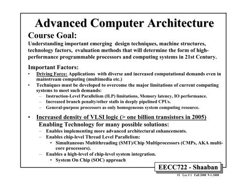
100000000Microprocessor Transistor CountGrowth Rate> One billion in 2005100000001000000Moore’s Lawi80386i80486PentiumAlpha 21264: 15 millionPentium Pro: 5.5 millionPowerPC 620: 6.9 millionAlpha 21164: 9.3 millionSparc Ultra: 5.2 million100000100001000i80286i8086i8080i40041970 1975 1980 1985 1990 1995 2000Moore’s Law:(circa 1970)2X transistors/ChipEvery 1.5 yearsStill valid todayYearHow to best exploit increased transistor count?• Keep increasing cache capacity/levels?• Multiple GPP cores?• Integrate other types of computing elements?~ 500,000x transistor density increasein the last 35 yearsEECC722 - Shaaban#11 Lec # 1 Fall 2008 9-1-2008

Microprocessor Frequency Trend10,000Mhz1,0001001038619871989486199121164A21064A210661993IntelIBM Power PCDECGate delays/clock21264S21264Pentium(R)21164 IIMPC750604 604+Pentium Pro601, 603 (R)Pentium(R)199519971999Processor freqscales by 2X pergeneration200120032005100101Gate Delays/ ClockRealty Check:Clock frequency scalingis slowing down!(Did silicone finally hitthe wall?)Why?1- Power leakage2- Clock distributiondelaysResult:Deeper PipelinesLonger stallsHigher CPI(lowers effectiveperformanceper cycle)1. Frequency used to double each generation2. Number of gates/clock reduce by 25%3. Leads to deeper pipelines with more stages(e.g Intel Pentium 4E has 30+ pipeline stages)T = I x CPI x CPossible Solutions?- Exploit Thread-Level Parallelism (TLP)at the chip level (SMT/CMP)- Utilize/integrate more-specializedcomputing elements other than GPPsEECC722 - Shaaban#12 Lec # 1 Fall 2008 9-1-2008

Parallelism in Microprocessor VLSI GenerationsTransistors100,000,00010,000,0001,000,000100,00010,000 i4004Bit-level parallelism Instruction-level Thread-level (?)Multiple micro-operationsper cycle(multi-cycle non-pipelined)Not PipelinedCPI >> 1 i8080i8008i80286 i8086(ILP)Single-issuePipelinedCPI =1i80386 R2000Single ThreadR10000 Pentium R3000Superscalar/VLIWCPI

Microprocessor Architecture TrendsGeneral Purpose Processor (GPP)CISC Machinesinstructions take variable times to completeSingleThreadedRISC Machines (microcode)simple instructions, optimized for speedRISC Machines (pipelined)same individual instruction latencygreater throughput through instruction "overlap"Multithreaded Processorsadditional HW resources (regs, PC, SP)each context gets processor for x cyclesSIMULTANEOUS MULTITHREADINGmultiple HW contexts (regs, PC, SP)each cycle, any context may executeSuperscalar Processorsmultiple instructions executing simultaneouslyVLIW"Superinstructions" grouped togetherdecreased HW control complexity(Single or Multi-Threaded)(SMT)CMPsSingle Chip Multiprocessorsduplicate entire processors(tech soon due to Moore's Law)(e.g IBM Power 4/5,AMD X2, X3, X4, Intel Core 2)e.g. Intel’s HyperThreading (P4)SMT/CMPse.g. IBM Power5,6,7 , Intel Pentium D, Sun Niagara - (UltraSparc T1)Upcoming (4 th quarter 2008) Intel Nehalem (Core I7)EECC722 - Shaaban#14 Lec # 1 Fall 2008 9-1-2008

Computer Technology Trends:Evolutionary but Rapid Change• Processor:– 1.5-1.6 performance improvement every year; Over 100X performance in lastdecade.• Memory:– DRAM capacity: > 2x every 1.5 years; 1000X size in last decade.– Cost per bit: Improves about 25% or more per year.– Only 15-25% performance improvement per year.• Disk:– Capacity: > 2X in size every 1.5 years.– Cost per bit: Improves about 60% per year.– 200X size in last decade.– Only 10% performance improvement per year, due to mechanical limitations.• Expected State-of-the-art PC by end of year 2008 :– Processor clock speed: ~ 3000 MegaHertz (3 Giga Hertz)– Memory capacity: > 8000 MegaByte (8 Giga Bytes)– Disk capacity: > 1000 GigaBytes (1 Tera Bytes)Performance gap comparedto CPU performance causessystem performance bottlenecksWith 2-4 processor coreson a single chipEECC722 - Shaaban#15 Lec # 1 Fall 2008 9-1-2008

Architectural Improvements• Increased optimization, utilization and size of cache systems withmultiple levels (currently the most popular approach to utilize theincreased number of available transistors) .• Memory-latency hiding techniques.• Optimization of pipelined instruction execution.• Dynamic hardware-based pipeline scheduling.• Improved handling of pipeline hazards.• Improved hardware branch prediction techniques.• Exploiting Instruction-Level Parallelism (ILP) in terms of multipleinstructionissue and multiple hardware functional units.• Inclusion of special instructions to handle multimedia applications.• High-speed system and memory bus designs to improve data transferrates and reduce latency.• Increased exploitation of Thread-Level Parallelism in terms ofSimultaneous Multithreading (SMT) and Chip Multiprocessors(CMPs)Including Simultaneous Multithreading (SMT)EECC722 - Shaaban#16 Lec # 1 Fall 2008 9-1-2008

Metrics of Computer Performance(Measures)ApplicationExecution time: Target workload,SPEC95, SPEC2000, etc.ProgrammingLanguageCompilerISA(millions) of Instructions per second – MIPS(millions) of (F.P.) operations per second – MFLOP/sDatapathControlFunction UnitsTransistors Wires PinsMegabytes per second.Cycles per second (clock rate).Each metric has a purpose, and each can be misused.EECC722 - Shaaban#17 Lec # 1 Fall 2008 9-1-2008

CPU Execution Time: The CPU Equation• A program is comprised of a number of instructions executed , I– Measured in: instructions/program• The average instruction executed takes a number of cycles perinstruction (CPI) to be completed.– Measured in: cycles/instruction, CPI• CPU has a fixed clock cycle time C = 1/clock rate– Measured in: seconds/cycle• CPU execution time is the product of the above threeparameters as follows: ExecutedCPU CPU time time = Seconds = Instructions x Cycles Cycles x SecondsProgramProgram Instruction Cycle Cycleexecution Timeper program in secondsT = I x CPI x CNumber ofinstructions executed(This equation is commonly known as the CPU performance equation)Average CPI for programOr Instructions Per Cycle (IPC):IPC= 1/CPICPU Clock CycleEECC722 - Shaaban#18 Lec # 1 Fall 2008 9-1-2008

Factors Affecting CPU PerformanceCPU CPU time time = Seconds = Instructions x Cycles Cycles x SecondsProgramProgram Instruction Cycle CycleProgramCompilerInstruction SetArchitecture (ISA)Organization(Micro-Architecture)TechnologyVLSIInstructionCount IXXXCPIIPCXXXXClock Cycle CXXT = I x CPI x CEECC722 - Shaaban#19 Lec # 1 Fall 2008 9-1-2008

Performance Enhancement Calculations:Amdahl's Law• The performance enhancement possible due to a given designimprovement is limited by the amount that the improved feature is used• Amdahl’s Law:Performance improvement or speedup due to enhancement E:Execution Time without E Performance with ESpeedup(E) = -------------------------------------- = ---------------------------------Execution Time with E Performance without E– Suppose that enhancement E accelerates a fraction F of theexecution time by a factor S and the remainder of the time isunaffected then:Execution Time with E = ((1-F) + F/S) X Execution Time without EHence speedup is given by:Execution Time without E 1Speedup(E) = --------------------------------------------------------- = --------------------((1 - F) + F/S) X Execution Time without E (1 - F) + F/SF (Fraction of execution time enhanced) refersto original execution time before the enhancement is appliedEECC722 - Shaaban#20 Lec # 1 Fall 2008 9-1-2008

Pictorial Depiction of Amdahl’s LawEnhancement E accelerates fraction F of original execution time by a factor of SBefore:Execution Time without enhancement E: (Before enhancement is applied)• shown normalized to 1 = (1-F) + F =1Unaffected fraction: (1- F)Affected fraction: FUnchangedUnaffected fraction: (1- F)After:Execution Time with enhancement E:F/SWhat if the fractions given areafter the enhancements were applied?How would you solve the problem?Execution Time without enhancement E 1Speedup(E) = ------------------------------------------------------ = ------------------Execution Time with enhancement E (1 - F) + F/SEECC722 - Shaaban#21 Lec # 1 Fall 2008 9-1-2008

Extending Amdahl's Law To Multiple Enhancements• Suppose that enhancement E i accelerates a fraction F i of theoriginal execution time by a factor S i and the remainder of thetime is unaffected then:Speedup=Unaffected fraction((1−∑iFiOriginal Execution Time) +∑i∑FSii)X1Speedup=((1−) +iFiOriginal Execution Time∑iFSiNote: All fractions F irefer to original execution time before theenhancements are applied..i)What if the fractions given areafter the enhancements were applied?How would you solve the problem?EECC722 - Shaaban#22 Lec # 1 Fall 2008 9-1-2008

Amdahl's Law With Multiple Enhancements:Example• Three CPU or system performance enhancements are proposed with thefollowing speedups and percentage of the code execution time affected:Speedup 1= S 1= 10 Percentage 1= F 1= 20%Speedup 2= S 2= 15 Percentage 1= F 2= 15%Speedup 3= S 3= 30 Percentage 1= F 3= 10%• While all three enhancements are in place in the new design, eachenhancement affects a different portion of the code and only oneenhancement can be used at a time.• What is the resulting overall speedup?Speedup=( ( 1 − )• Speedup = 1 / [(1 - .2 - .15 - .1) + .2/10 + .15/15 + .1/30)]= 1 / [ .55 + .0333 ]= 1 / .5833 = 1.71∑iF1i+∑iFSii)EECC722 - Shaaban#23 Lec # 1 Fall 2008 9-1-2008

Pictorial Depiction of ExampleBefore:Execution Time with no enhancements: 1UnchangedS 1= 10 S 2= 15 S 3= 30Unaffected, fraction: .55 F 1 = .2 F 2 = .15 F 3 = .1/ 10 / 15 / 30Unaffected, fraction: .55After:Execution Time with enhancements: .55 + .02 + .01 + .00333 = .5833Speedup = 1 / .5833 = 1.71Note: All fractions (F i, i = 1, 2, 3) refer to original execution time.What if the fractions given areafter the enhancements were applied?How would you solve the problem?EECC722 - Shaaban#24 Lec # 1 Fall 2008 9-1-2008

“Reverse” Multiple Enhancements Amdahl's Law• Multiple Enhancements Amdahl's Law assumes that the fractions givenrefer to original execution time.• If for each enhancement S i the fraction F i it affects is given as a fractionof the resulting execution time after the enhancements were appliedthen:SpeedupUnaffected fraction(( F F S X∑ ∑=(1 − ) + × ) Resulting Execution Timei i i i iResulting Execution Time1−∑ F ) + ∑ F × Si i i i i= = ( 1−∑F ) + ∑i iSpeedup F ×i i1i.e as if resulting execution time is normalized to 1• For the previous example assuming fractions given refer to resultingexecution time after the enhancements were applied (not the originalexecution time), then:Speedup = (1 - .2 - .15 - .1) + .2 x10 + .15 x15 + .1x30= .55 + 2 + 2.25 + 3= 7.8SEECC722 - Shaaban#25 Lec # 1 Fall 2008 9-1-2008i

Instruction Pipelining Review• Instruction pipelining is CPU implementation technique where multipleoperations on a number of instructions are overlapped.– Instruction pipelining exploits Instruction-Level Parallelism (ILP)• An instruction execution pipeline involves a number of steps, where each stepcompletes a part of an instruction. Each step is called a pipeline stage or a pipelinesegment.• The stages or steps are connected in a linear fashion: one stage to the next toform the pipeline -- instructions enter at one end and progress through the stagesand exit at the other end. 1 2 3 4 5• The time to move an instruction one step down the pipeline is is equal to themachine cycle and is determined by the stage with the longest processing delay.• Pipelining increases the CPU instruction throughput: The number of instructionscompleted per cycle.– Under ideal conditions (no stall cycles), instruction throughput is oneinstruction per machine cycle, or ideal CPI = 1 Or IPC = 1• Pipelining does not reduce the execution time of an individual instruction: Thetime needed to complete all processing steps of an instruction (also calledinstruction completion latency). Pipelining may actually increase individual instruction latency– Minimum instruction latency = n cycles, where n is the number of pipelinestagesThe pipeline described here is called an in-order pipeline because instructionsare processed or executed in the original program orderEECC722 - Shaaban#26 Lec # 1 Fall 2008 9-1-2008

MIPS In-Order Single-Issue Integer PipelineIdeal Operation(No stall cycles)Fill Cycles = number of stages -1(Classic 5-Stage)Program OrderClock Number Time in clock cycles →Instruction Number 1 2 3 4 5 6 7 8 9Instruction I IF ID EX MEM WBInstruction I+1 IF ID EX MEM WBInstruction I+2 IF ID EX MEM WBInstruction I+3IF ID EX MEM WBInstruction I +4 IF ID EX MEM WB4 cycles = n -1Time to fill the pipelineMIPS Pipeline Stages:IF = Instruction FetchID = Instruction DecodeEX = ExecutionMEM = Memory AccessWB = Write BackFirst instruction, ICompletedIn-order = instructions executed in original program orderIdeal pipeline operation without any stall cyclesLast instruction,I+4 completedn= 5 pipeline stages Ideal CPI =1(or IPC =1)EECC722 - Shaaban#27 Lec # 1 Fall 2008 9-1-2008

A Pipelined MIPS Datapath• Obtained from multi-cycle MIPS datapath by adding buffer registers between pipeline stages• Assume register writes occur in first half of cycle and register reads occur in second half.IFStage 1IDEXStage 2 Stage 3Branches resolvedHere in MEM (Stage 4)MEMStage 4WBStage 5Classic Five StageInteger Single-IssueIn-Order PipelineBranch Penalty = 4 -1 = 3 cyclesEECC722 - Shaaban#28 Lec # 1 Fall 2008 9-1-2008

ResourceNot available:Pipeline Hazards• Hazards are situations in pipelining which prevent the nextinstruction in the instruction stream from executing duringthe designated clock cycle possibly resulting in one or morestall (or wait) cycles.• Hazards reduce the ideal speedup (increase CPI > 1) gainedfrom pipelining and are classified into three classes:HardwareComponentCorrectOperand(data) valueCorrectPCi.e A resource the instruction requires for correctexecution is not available in the cycle needed– Structural hazards: Arise from hardware resource conflictswhen the available hardware cannot support all possiblecombinations of instructions.– Data hazards: Arise when an instruction depends on theresult of a previous instruction in a way that is exposed by theoverlapping of instructions in the pipeline– Control hazards: Arise from the pipelining of conditionalbranches and other instructions that change the PCCorrect PC not available when needed in IFHardware structure (component) conflictOperand not ready yetwhen needed in EXEECC722 - Shaaban#29 Lec # 1 Fall 2008 9-1-2008

One shared memory forinstructions and dataMIPS with MemoryUnit Structural HazardsEECC722 - Shaaban#30 Lec # 1 Fall 2008 9-1-2008

CPI = 1 + stall clock cycles per instruction = 1 + fraction of loads and stores x 1One shared memory forinstructions and dataStall or waitCycleResolving A StructuralHazard with StallingInstructions 1-3 above are assumed to be instructions other than loads/storesEECC722 - Shaaban#31 Lec # 1 Fall 2008 9-1-2008

Data Hazards• Data hazards occur when the pipeline changes the order ofread/write accesses to instruction operands in such a way thatthe resulting access order differs from the original sequentialinstruction operand access order of the unpipelined machineresulting in incorrect execution.• Data hazards may require one or more instructions to bestalled to ensure correct execution.• Example:12345DADD R1, R2, R3DSUB R4, R1, R5AND R6, R1, R7OR R8,R1,R9XOR R10, R1, R11– All the instructions after DADD use the result of the DADD instruction– DSUB, AND instructions need to be stalled for correct execution.i.e Correct operand data not ready yet when needed in EX cycleCPI = 1 + stall clock cycles per instructionArrows represent data dependenciesbetween instructionsInstructions that have no dependencies amongthem are said to be parallel or independentA high degree of Instruction-Level Parallelism (ILP)is present in a given code sequence if it has a largenumber of parallel instructionsEECC722 - Shaaban#32 Lec # 1 Fall 2008 9-1-2008

12345DataHazard ExampleFigure A.6 The use of the result of the DADD instruction in the next three instructionscauses a hazard, since the register is not written until after those instructions read it.Two stall cycles are needed here(to prevent data hazard)EECC722 - Shaaban#33 Lec # 1 Fall 2008 9-1-2008

Minimizing Data hazard Stalls by Forwarding• Data forwarding is a hardware-based technique (also calledregister bypassing or short-circuiting) used to eliminate orminimize data hazard stalls.• Using forwarding hardware, the result of an instruction is copieddirectly from where it is produced (ALU, memory read portetc.), to where subsequent instructions need it (ALU inputregister, memory write port etc.)• For example, in the MIPS integer pipeline with forwarding:– The ALU result from the EX/MEM register may be forwarded or fedback to the ALU input latches as needed instead of the registeroperand value read in the ID stage.– Similarly, the Data Memory Unit result from the MEM/WB registermay be fed back to the ALU input latches as needed .– If the forwarding hardware detects that a previous ALU operation is towrite the register corresponding to a source for the current ALUoperation, control logic selects the forwarded result as the ALU inputrather than the value read from the register file.EECC722 - Shaaban#34 Lec # 1 Fall 2008 9-1-2008

1Forward2Forward345Pipelinewith ForwardingA set of instructions that depend on the DADD result uses forwarding paths to avoid the data hazardEECC722 - Shaaban#35 Lec # 1 Fall 2008 9-1-2008

I (Write)Data Hazard/Dependence ClassificationI (Read)True Data DependenceJ (Read)SharedOperandRead after Write (RAW)if data dependence is violatedI (Write)I....JProgramOrderA name dependence:antidependenceJ (Write)SharedOperandWrite after Read (WAR)if antidependence is violatedI (Read)Or nameA name dependence:output dependenceSharedOperandNo dependenceSharedOperandJ (Write)Or nameJ (Read)Write after Write (WAW)if output dependence is violatedRead after Read (RAR) not a hazardEECC722 - Shaaban#36 Lec # 1 Fall 2008 9-1-2008

Control Hazards• When a conditional branch is executed it may change the PC and,without any special measures, leads to stalling the pipeline for a numberof cycles until the branch condition is known (branch is resolved).– Otherwise the PC may not be correct when needed in IF• In current MIPS pipeline, the conditional branch is resolved in stage 4(MEM stage) resulting in three stall cycles as shown below:Branch instruction IF ID EX MEM WBBranch successor stall stall stall IF ID EX MEM WBBranch successor + 1IF ID EX MEM WBBranch successor + 2IF ID EX MEM3 stall cyclesBranch successor + 3IF ID EXBranch successor + 4IF IDBranch PenaltyBranch successor + 5IFAssuming we stall or flush the pipeline on a branch instruction:Three clock cycles are wasted for every branch for current MIPS pipelineBranch Penalty = stage number where branch is resolved - 1here Branch Penalty = 4 - 1 = 3 Cyclesi.e Correct PC is not available when needed in IFCorrect PC available here(end of MEM cycle or stage)EECC722 - Shaaban#37 Lec # 1 Fall 2008 9-1-2008

Pipeline Performance Example• Assume the following MIPS instruction mix:TypeFrequencyArith/Logic 40%Load30% of which 25% are followed immediately byan instruction using the loaded valueStore 10%branch 20% of which 45% are taken 1 stall1 stall• What is the resulting CPI for the pipelined MIPS withforwarding and branch address calculation in ID stagewhen using a branch not-taken scheme?• CPI = Ideal CPI + Pipeline stall clock cycles per instruction= 1 + stalls by loads + stalls by branches= 1 + .3 x .25 x 1 + .2 x .45 x 1= 1 + .075 + .09= 1.165Branch Penalty = 1 cycleEECC722 - Shaaban#38 Lec # 1 Fall 2008 9-1-2008

Pipelining and ExploitingInstruction-Level Parallelism (ILP)• Instruction-Level Parallelism (ILP) exists when instructions in a sequenceare independent and thus can be executed in parallel by overlapping.– Pipelining increases performance by overlapping the execution ofindependent instructions and thus exploits ILP in the code.• Preventing instruction dependency violations (hazards) may result in stallcycles in a pipelined CPU increasing its CPI (reducing performance).– The CPI of a real-life pipeline is given by (assuming ideal memory):Pipeline CPI = Ideal Pipeline CPI + Structural Stalls + RAW Stalls+ WAR Stalls + WAW Stalls + Control Stalls• Programs that have more ILP (fewer dependencies) tend to performbetter on pipelined CPUs.– More ILP mean fewer instruction dependencies and thus fewer stallcycles needed to prevent instruction dependency violations i.e hazardsIn Fourth Edition Chapter 2.1(In Third Edition Chapter 3.1)i.e non-idealDependency Violation = Hazardi.e instruction throughputT = I x CPI x C(without stalling)EECC722 - Shaaban#39 Lec # 1 Fall 2008 9-1-2008

Basic Instruction Block• A basic instruction block is a straight-line code sequence with nobranches in, except at the entry point, and no branches outexcept at the exit point of the sequence. Start of Basic BlockBasic– Example: Body of a loop. End of Basic BlockBlock• The amount of instruction-level parallelism (ILP) in a basicblock is limited by instruction dependence present and size ofthe basic block.• In typical integer code, dynamic branch frequency is about 15%(resulting average basic block size of about 7 instructions).• Any static technique that increases the average size of basicblocks which increases the amount of exposed ILP in the codeand provide more instructions for static pipeline scheduling bythe compiler possibly eliminating more stall cycles and thusimproves pipelined CPU performance.– Loop unrolling is one such technique that we examine nextBranch In: :: :Branch (out)In Fourth Edition Chapter 2.1 (In Third Edition Chapter 3.1)Static = At compilation time Dynamic = At run timeEECC722 - Shaaban#40 Lec # 1 Fall 2008 9-1-2008

Basic Blocks/Dynamic Execution Sequence (Trace) ExampleStatic ProgramOrderABDH.EJ.I.K.CFL.GṆ.• A-O = Basic Blocks terminating with conditionalbranches• The outcomes of branches determine the basicblock dynamic execution sequence or traceProgram Control Flow Graph (CFG)Trace: Dynamic Sequence of basic blocks executedIf all three branches are takenthe execution trace will be basicblocks: ACGOM.ONT = Branch Not TakenT = Branch TakenType of branches in this example:“If-Then-Else” branches (not loops)Average Basic Block Size = 5-7 instructionsEECC722 - Shaaban#41 Lec # 1 Fall 2008 9-1-2008

Increasing Instruction-Level Parallelism (ILP)• A common way to increase parallelism among instructions is toexploit parallelism among iterations of a loop– (i.e Loop Level Parallelism, LLP). Or Data Parallelism in a loop• This is accomplished by unrolling the loop either statically by thecompiler, or dynamically by hardware, which increases the size ofthe basic block present. This resulting larger basic blockprovides more instructions that can be scheduled or re-orderedby the compiler to eliminate more stall cycles.• In this loop every iteration can overlap with any other iteration.Overlap within each iteration is minimal.Example:Independent (parallel) loop iterations:A result of high degree of data parallelismfor (i=1; i

MIPS Loop Unrolling Example• For the loop:Note:IndependentLoop Iterationsfor (i=1000; i>0; i=i-1)x[i] = x[i] + s;R1 initiallypoints hereR1 -8 points hereR2 +8 points hereR2 points hereHigh MemoryX[1000]X[999]The straightforward MIPS assembly code is given by:X[1]....Low MemoryFirst element tocomputeLast element tocomputeProgram OrderLoop: L.D F0, 0 (R1) ;F0=array elementADD.D F4, F0, F2 ;add scalar in F2 (constant)S.D F4, 0(R1) ;store resultDADDUI R1, R1, # -8 ;decrement pointer 8 bytesBNE R1, R2,Loop ;branch R1!=R2SR1 is initially the address of the element with highest address.8(R2) is the address of the last element to operate on.X[ ] array of double-precision floating-point numbers (8-bytes each)In Fourth Edition Chapter 2.2(In Third Edition Chapter 4.1)Initial value of R1 = R2 + 8000Basic block size = 5 instructionsEECC722 - Shaaban#43 Lec # 1 Fall 2008 9-1-2008

MIPS FP Latency AssumptionsFor Loop Unrolling Examplei.e 4 execution(EX) cycles forFP instructions• All FP units assumed to be pipelined.• The following FP operations latencies are used:InstructionProducing ResultFP ALU Opi.e followed immediately by ..InstructionUsing ResultAnother FP ALU Op(or Number ofStall Cycles)Latency InClock Cycles3FP ALU OpLoad DoubleLoad DoubleStore DoubleFP ALU OpStore Double210Other Assumptions:- Branch resolved in decode stage, Branch penalty = 1 cycle- Full forwarding is used- Single Branch delay Slot- Potential structural hazards ignoredIn Fourth Edition Chapter 2.2 (In Third Edition Chapter 4.1)EECC722 - Shaaban#44 Lec # 1 Fall 2008 9-1-2008

Program OrderDue toresolvingbranchin IDLoop Unrolling Example (continued)• This loop code is executed on the MIPS pipeline as follows:(Branch resolved in decode stage, Branch penalty = 1 cycle, Full forwarding is used)No scheduling(Resulting stalls shown)Clock cycleLoop: L.D F0, 0(R1) 1stall 2ADD.D F4, F0, F2 3stall 4stall 5S.D F4, 0 (R1) 6DADDUI R1, R1, # -8 7stall 8BNE R1,R2, Loop 9stall 1010 cycles per iterationIn Fourth Edition Chapter 2.2(In Third Edition Chapter 4.1)• Ignoring Pipeline Fill Cycles• No Structural HazardsScheduled with single delayedbranch slot:(Resulting stalls shown)Loop: L.D F0, 0(R1)DADDUI R1, R1, # -8ADD.D F4, F0, F2stallBNE R1,R2, LoopS.D F4,8(R1)S.D in branch delay slot6 cycles per iteration10/6 = 1.7 times fasterEECC722 - Shaaban#45 Lec # 1 Fall 2008 9-1-2008Cycle123456

Iteration1234CycleNo schedulingLoop: 1 L.D F0, 0(R1)2345678910111213141516171819202122232425262728StallADD.D F4, F0, F2StallStallSD F4,0 (R1)LD F6, -8(R1)StallADDD F8, F6, F2StallStallSD F8, -8 (R1),Loop Unrolling Example (continued)• The resulting loop code when four copies of theloop body are unrolled without reuse of registers.• The size of the basic block increased from 5instructions in the original loop to 14 instructions.; drop DADDUI & BNE; drop DADDUI & BNELD F10, -16(R1)StallADDD F12, F10, F2StallStallSD F12, -16 (R1) ; drop DADDUI & BNELD F14, -24 (R1)StallADDD F16, F14, F2StallStallSD F16, -24(R1)DADDUI R1, R1, # -32StallBNE R1, R2, LoopStallIn Fourth Edition Chapter 2.2(In Third Edition Chapter 4.1)Loop unrolled 4 times(Resulting stalls shown)New Basic Block Size = 14 Instructionsi.e. unrolled four timesNote use of different registers for each iteration (register renaming)Three branches and threedecrements of R1 are eliminated.Load and store addresses arechanged to allow DADDUIinstructions to be merged.Performance:The unrolled loop runs in 28 cyclesassuming each L.D has 1 stallcycle, each ADD.D has 2 stallcycles, the DADDUI 1 stall, thebranch 1 stall cycle, or 28/4 = 7cycles to produce each of the fourelements.EECC722 - Shaaban#46 Lec # 1 Fall 2008 9-1-2008RegisterRenamingUsedi.e 7 cycles for each original iteration

Program OrderNote: No stallsLoop Unrolling Example (continued)When scheduled for pipelineLoop: L.D F0, 0(R1)L.D F6,-8 (R1)L.D F10, -16(R1)L.D F14, -24(R1)ADD.D F4, F0, F2ADD.D F8, F6, F2ADD.D F12, F10, F2ADD.D F16, F14, F2S.D F4, 0(R1)S.D F8, -8(R1)DADDUI R1, R1,# -32S.D F12, 16(R1),F12BNE R1,R2, LoopS.D F16, 8(R1), F16 ;8-32 = -24In Fourth Edition Chapter 2.2(In Third Edition Chapter 4.1)In branch delay slotThe execution time of the loophas dropped to 14 cycles, or 14/4 = 3.5clock cycles per elementcompared to 7 before schedulingand 6 when scheduled but unrolled.Speedup = 6/3.5 = 1.7i.e 3.5 cycles for eachoriginal iterationi.e more ILPexposedUnrolling the loop exposed morecomputations that can be scheduledto minimize stalls by increasing thesize of the basic block from 5 instructionsin the original loop to 14 instructionsin the unrolled loop.Larger Basic Block More ILPExposedEECC722 - Shaaban#47 Lec # 1 Fall 2008 9-1-2008

Loop-Level Level Parallelism (LLP) Analysis• Loop-Level Parallelism (LLP) analysis focuses on whether data accesses in lateriterations of a loop are data dependent on data values produced in earlieriterations and possibly making loop iterations independent (parallel).e.g. in for (i=1; i

LLP Analysis Example 1• In the loop:for (i=1; i

LLP Analysis Example 2• In the loop:i.e. loopDependency Graphfor (i=1; i

S1Original Loop:A[1] = A[1] + B[1];LLP Analysis Example 2for (i=1; i

Why?Reduction of Data Hazards Stallswith Dynamic Scheduling• So far we have dealt with data hazards in instruction pipelines by:– Result forwarding (register bypassing) to reduce or eliminate stalls neededto prevent RAW hazards as a result of true data dependence.– Hazard detection hardware to stall the pipeline starting with the instructionthat uses the result. i.e forward + stall (if needed)– Compiler-based static pipeline scheduling to separate the dependentinstructions minimizing actual hazard-prevention stalls in scheduled code.• Loop unrolling to increase basic block size: More ILP exposed.i.e Start of instruction execution is not in program order• Dynamic scheduling: (out-of-order execution)– Uses a hardware-based mechanism to reorder or rearrange instructionexecution order to reduce stalls dynamically at runtime.• Better dynamic exploitation of instruction-level parallelism (ILP).– Enables handling some cases where instruction dependencies are unknownat compile time (ambiguous dependencies).– Similar to the other pipeline optimizations above, a dynamically scheduledprocessor cannot remove true data dependencies, but tries to avoid orreduce stalling.Fourth Edition: Appendix A.7, Chapter 2.4, 2.5(Third Edition: Appendix A.8, Chapter 3.2, 3.3)EECC722 - Shaaban#52 Lec # 1 Fall 2008 9-1-2008

Dynamic Pipeline Scheduling: The Concept• Dynamic pipeline scheduling overcomes the limitations of in-orderpipelined execution by allowing out-of-order instruction execution.• Instruction are allowed to start executing out-of-order as soon astheir operands are available.• Better dynamic exploitation of instruction-level parallelism (ILP).Example:(Out-of-order execution)In the case of in-order pipelined executionSUB.D must wait for DIV.D to completewhich stalled ADD.D before starting executionIn out-of-order execution SUBD can start as soonas the values of its operands F8, F14 are available.DIV.D F0, F2, F4ADD.D F10, F0, F8SUB.D F12, F8, F14• This implies allowing out-of-order instruction commit (completion).• May lead to imprecise exceptions if an instruction issued earlierraises an exception.– This is similar to pipelines with multi-cycle floating point units.In Fourth Edition: Appendix A.7, Chapter 2.4(In Third Edition: Appendix A.8, Chapter 3.2)i.e Start of instruction execution is not in program orderTrue DataDependencyProgram OrderOrder = Program Instruction Order123Does not depend on DIV.D or ADD.DEECC722 - ShaabanDependencyGraph#53 Lec # 1 Fall 2008 9-1-2008123

Dynamic Scheduling:The Tomasulo Algorithm• Developed at IBM and first implemented in IBM’s 360/91mainframe in 1966, about 3 years after the debut of the scoreboardin the CDC 6600.• Dynamically schedule the pipeline in hardware to reduce stalls.• Differences between IBM 360 & CDC 6600 ISA.– IBM has only 2 register specifiers/instr vs. 3 in CDC 6600.– IBM has 4 FP registers vs. 8 in CDC 6600.• Current CPU architectures that can be considered descendants ofthe IBM 360/91 which implement and utilize a variation of theTomasulo Algorithm include:RISC CPUs: Alpha 21264, HP 8600, MIPS R12000, PowerPC G4RISC-core x86 CPUs: AMD Athlon, Pentium III, 4, Xeon ….In Fourth Edition: Chapter 2.4(In Third Edition: Chapter 3.2)EECC722 - Shaaban#54 Lec # 1 Fall 2008 9-1-2008

Dynamic Scheduling: The Tomasulo ApproachInstructions to Issue(in program order)(Instruction Fetch)(IQ)The basic structure of a MIPS floating-point unit using Tomasulo’s algorithmIn Fourth Edition: Chapter 2.4(In Third Edition: Chapter 3.2)Pipelined FP units are used hereEECC722 - Shaaban#55 Lec # 1 Fall 2008 9-1-2008

Alwaysdone inprogramorderCan bedoneout ofprogramorderThree Stages of Tomasulo Algorithm1 Issue: Get instruction from pending Instruction Queue (IQ).– Instruction issued to a free reservation station(RS) (no structural hazard).– Selected RS is marked busy.– Control sends available instruction operands values (from ISA registers)to assigned RS.– Operands not available yet are renamed to RSs that will produce theoperand (register renaming). (Dynamic construction of data dependency graph)2 Execution (EX): Operate on operands.– When both operands are ready then start executing on assigned FU.– If all operands are not ready, watch Common Data Bus (CDB) for neededresult (forwarding done via CDB). (i.e. wait on any remaining operands, no RAW)3 Write result (WB): Finish execution.– Write result on Common Data Bus (CDB) to all awaiting units (RSs)– Mark reservation station as available.• Normal data bus: data + destination (“go to” bus).• Common Data Bus (CDB): data + source (“come from” bus):– 64 bits for data + 4 bits for Functional Unit source address.In Fourth Edition: Chapter 2.4(In Third Edition: Chapter 3.2)– Write data to waiting RS if source matches expected RS (that produces result).– Does the result forwarding via broadcast to waiting RSs.Including destination registerStage 0 Instruction Fetch (IF): No changes, in-orderAlso includes waiting for operands + MEMData dependencies observedi.e broadcast result on CDB forwarding)Note: No WB for storesEECC722 - Shaaban#56 Lec # 1 Fall 2008 9-1-2008

How?BTBDynamic Conditional Branch Prediction• Dynamic branch prediction schemes are different from static mechanismsbecause they utilize hardware-based mechanisms that use the run-timebehavior of branches to make more accurate predictions than possible usingstatic prediction.• Usually information about outcomes of previous occurrences of branches(branching history) is used to dynamically predict the outcome of thecurrent branch. Some of the proposed dynamic branch predictionmechanisms include:– One-level or Bimodal: Uses a Branch History Table (BHT), a table ofusually two-bit saturating counters which is indexed by a portion of thebranch address (low bits of address). (First proposed mid 1980s)– Two-Level Adaptive Branch Prediction. (First proposed early 1990s),– MCFarling’s Two-Level Prediction with index sharing (gshare, 1993).– Hybrid or Tournament Predictors: Uses a combinations of two or more(usually two) branch prediction mechanisms (1993).• To reduce the stall cycles resulting from correctly predicted taken branchesto zero cycles, a Branch Target Buffer (BTB) that includes the addresses ofconditional branches that were taken along with their targets is added to thefetch stage.4 th Edition: Static and Dynamic Prediction in ch. 2.3, BTB in ch. 2.9(3 rd Edition: Static Pred. in Ch. 4.2 Dynamic Pred. in Ch. 3.4, BTB in Ch. 3.5)EECC722 - Shaaban#57 Lec # 1 Fall 2008 9-1-2008

Branch Target Buffer (BTB)• Effective branch prediction requires the target of the branch at an earlypipeline stage. (resolve the branch early in the pipeline)– One can use additional adders to calculate the target, as soon as the branchinstruction is decoded. This would mean that one has to wait until the ID stagebefore the target of the branch can be fetched, taken branches would be fetched witha one-cycle penalty (this was done in the enhanced MIPS pipeline Fig A.24).• To avoid this problem and to achieve zero stall cycles for taken branches, onecan use a Branch Target Buffer (BTB).• A typical BTB is an associative memory where the addresses of taken branchinstructions are stored together with their target addresses.• The BTB is is accessed in Instruction Fetch (IF) cycle and provides answers tothe following questions while the current instruction is being fetched:1 – Is the instruction a branch?2 – If yes, is the branch predicted taken?3 – If yes, what is the branch target?• Instructions are fetched from the target stored in the BTB in case the branch ispredicted-taken and found in BTB.• After the branch has been resolved the BTB is updated. If a branch isencountered for the first time a new entry is created once it is resolved as taken.Goal of BTB: Zero stall taken branchesEECC722 - Shaaban#58 Lec # 1 Fall 2008 9-1-2008

Basic Branch Target Buffer (BTB)Is the instruction a branch?(for address match)Fetch instruction frominstruction memory (I-L1 Cache)InstructionFetchIFBranch AddressBranch Targetif predicted takenBranchTaken?Branch TargetsBTB is accessed in Instruction Fetch (IF) cycleGoal of BTB: Zero stall taken branches0 = NT = Not Taken1 = T = TakenEECC722 - Shaaban#59 Lec # 1 Fall 2008 9-1-2008

One-Level (Bimodal) Branch Predictors• One-level or bimodal branch prediction uses only one level of branchhistory.• These mechanisms usually employ a table which is indexed by lowerN bits of the branch address. Pattern History Table (PHT)• Each table entry (or predictor) consists of n history bits, whichform an n-bit automaton or saturating counters.• Smith proposed such a scheme, known as the Smith Algorithm, thatuses a table of two-bit saturating counters. (1985)• One rarely finds the use of more than 3 history bits in the literature.• Two variations of this mechanism:– Pattern History Table: Consists of directly mapped entries.– Branch History Table (BHT): Stores the branch address as a tag. Itis associative and enables one to identify the branch instructionduring IF by comparing the address of an instruction with thestored branch addresses in the table (similar to BTB).PHTEECC722 - Shaaban#60 Lec # 1 Fall 2008 9-1-2008

One-Level Bimodal Branch PredictorsPattern History Table (PHT)Most common one-level implementationSometimes referred to asDecode History Table (DHT)orBranch History Table (BHT)N Low Bits of2-bit saturating counters (predictors)High bit determinesbranch prediction0 = NT = Not Taken1 = T = TakenTable has 2 N entries(also called predictors) . 0 0Example:For N =12Table has 2 N = 2 12 entries= 4096 = 4k entriesNumber of bits needed = 2 x 4k = 8k bitsWhat if different branches map to the same predictor (counter)?This is called branch address aliasing and leads to interference with current branch prediction by other branchesand may lower branch prediction accuracy for programs with aliasing.0 11 01 1Not Taken(NT)Taken(T)Update counter after branch is resolved:-Increment counter used if branch is taken- Decrement counter used if branch is nottakenEECC722 - Shaaban#61 Lec # 1 Fall 2008 9-1-2008

FPN=122 N = 4096Prediction Accuracy ofA 4096-Entry Basic One-Level Dynamic Two-BitBranch PredictorIntegerMisprediction Rate:Integer average 11%FP average 4%(Lower misprediction ratedue to more loops)Has, more branchesinvolved inIF-Then-Elseconstructs than FPEECC722 - Shaaban#62 Lec # 1 Fall 2008 9-1-2008

aa=bb=2Correlating BranchesRecent branches are possibly correlated: The behavior ofrecently executed branches affects prediction of currentbranch.Example:B1B2B3if (aa==2)aa=0;if (bb==2)bb=0;if (aa!==bb){DSUBUI R3, R1, #2 ; R3 = R1 - 2BNEZ R3, L1 ; B1 (aa!=2)DADD R1, R0, R0 ; aa==0L1: DSUBUI R3, R2, #2 ; R3 = R2 - 2BNEZ R3, L2 ; B2 (bb!=2)DADD R2, R0, R0 ; bb==0L2: DSUBUI R3, R1, R2 ; R3=aa-bbBEQZ R3, L3 ; B3 (aa==bb)Branch B3 is correlated with branches B1, B2. If B1, B2 areboth not taken, then B3 will be taken. Using only the behaviorof one branch cannot detect this behavior.B3 in this case(not taken)(not taken)(not taken)Occur in branches used to implement if-then-else constructsWhich are more common in integer than floating point codeHere aa = R1 bb = R2B1 not takenB2 not takenB3 taken if aa=bbEECC722 - Shaaban#63 Lec # 1 Fall 2008 9-1-2008

Correlating Two-Level Dynamic GAp Branch Predictors• Improve branch prediction by looking not only at the history of the branch inquestion but also at that of other branches using two levels of branch history.• Uses two levels of branch history:12m-bit shift registerBranch History Register (BHR)LastBranch0 =Not taken1 = Taken– First level (global):• Record the global pattern or history of the m most recently executedbranches as taken or not taken. Usually an m-bit shift register.– Second level (per branch address): Pattern History Tables (PHTs)• 2 m prediction tables (PHTs), each table entry has n bit saturatingcounter.• The branch history pattern from first level is used to select the properbranch prediction table in the second level.• The low N bits of the branch address are used to select the correctprediction entry (predictor)within a the selected table, thus each of the2 m tables has 2 N entries and each entry is 2 bits counter.• Total number of bits needed for second level = 2 m x n x 2 N bits• In general, the notation: GAp (m,n) predictor means:– Record last m branches to select between 2 m history tables.– Each second level table uses n-bit counters (each table entry has n bits).• Basic two-bit single-level Bimodal BHT is then a (0,2) predictor.4 th Edition: In Chapter 2.3 (3 rd Edition: In Chapter 3.4)EECC722 - Shaaban#64 Lec # 1 Fall 2008 9-1-2008

(N= 4)SelectscorrectEntry(predictor)in tableLow 4 bits of address(n = 2)Organization of A Correlating TwolevelGAp (2,2) Branch PredictorSecond LevelPattern History Tables (PHTs)High bit determinesbranch prediction0 = Not Taken1 = TakenGlobal(1st level)GApm = # of branches tracked in first level = 2Thus 2 m = 2 2 = 4 tables in second levelAdaptiveper address(2nd level)Selects correcttableBranch HistoryRegister (BHR)First LevelBranch HistoryRegister (BHR)(2 bit shift register)(m = 2)N = # of low bits of branch address used = 4Thus each table in 2nd level has 2N = 24 = 16entriesn = # number of bits of 2nd level table entry = 2Number of bits for 2nd level = 2 m x n x 2 N= 4 x 2 x 16 = 128 bitsEECC722 - Shaaban#65 Lec # 1 Fall 2008 9-1-2008

N = 12 N = 10FPIntegerBasicSingle (one) LevelBasicCorrelatingTwo-levelGap (2, 2)m= 2 n= 2Prediction Accuracyof Two-Bit DynamicPredictors UnderSPEC89EECC722 - Shaaban#66 Lec # 1 Fall 2008 9-1-2008

Multiple Instruction Issue: CPI < 1• To improve a pipeline’s CPI to be better [less] than one, and to better exploitInstruction Level Parallelism (ILP), a number of instructions have to be issued inthe same cycle.• Multiple instruction issue processors are of two types:– Superscalar: A number of instructions (2-8) is issued in the samecycle, scheduled statically by the compiler or -more commonlydynamically(Tomasulo).• PowerPC, Sun UltraSparc, Alpha, HP 8000, Intel PII, III, 4 ...– VLIW (Very Long Instruction Word):A fixed number of instructions (3-6) are formatted as one longinstruction word or packet (statically scheduled by the compiler).– Example: Explicitly Parallel Instruction Computer (EPIC)• Originally a joint HP/Intel effort.• ISA: Intel Architecture-64 (IA-64) 64-bit address:• First CPU: Itanium, Q1 2001. Itanium 2 (2003)• Limitations of the approaches:– Available ILP in the program (both).– Specific hardware implementation difficulties (superscalar).– VLIW optimal compiler design issues.CPI < 1 or Instructions Per Cycle (IPC) > 1Most common = 4 instructions/cyclecalled 4-way superscalar processor4 th Edition: Chapter 2.7(3 rd Edition: Chapter 3.6, 4.3EECC722 - Shaaban#67 Lec # 1 Fall 2008 9-1-2008

Simple Statically Scheduled Superscalar Pipeline• Two instructions can be issued per cycle (static two-issue or 2-way superscalar).• One of the instructions is integer (including load/store, branch). The other instructionis a floating-point operation.– This restriction reduces the complexity of hazard checking.• Hardware must fetch and decode two instructions per cycle.• Then it determines whether zero (a stall), one or two instructions can be issued (indecode stage) per cycle.Instruction TypeInteger InstructionFP InstructionInteger InstructionFP InstructionInteger InstructionFP InstructionInteger InstructionFP Instruction1 2 3 4 5 6 7 8IFIFIDIDIFIFEXEXIDIDIFIFMEMEXEXEXIDIDIFIFTwo-issue statically scheduled pipeline in operationFP instructions assumed to be adds (EX takes 3 cycles)Ideal CPI = 0.5 Ideal Instructions Per Cycle (IPC) = 2WBEXMEMEXEXEXIDIDWBWBEXMEMEXEXEXWBWBEXMEMEXWBWBEXInstructions assumed independent (no stalls)EECC722 - Shaaban#68 Lec # 1 Fall 2008 9-1-2008

Intel IA-64: VLIW “Explicitly ParallelInstruction Computing (EPIC)”• Three 41-bit instructions in 128 bit “Groups” or bundles;an instruction bundle template field (5-bits) determines ifinstructions are dependent or independent and statically specifiesthe functional units to used by the instructions:– Smaller code size than old VLIW, larger than x86/RISC– Groups can be linked to show dependencies of more than threeinstructions.• 128 integer registers + 128 floating point registers• Hardware checks dependencies(interlocks ⇒ binary compatibility over time)• Predicated execution: An implementation of conditionalinstructions used to reduce the number of conditional branchesused in the generated code ⇒ larger basic block size• IA-64 : Name given to instruction set architecture (ISA).• Itanium : Name of the first implementation (2001).In VLIW dependency analysis is done statically by the compilernot dynamically in hardware (Tomasulo)i.e statically scheduledby compilerStatically scheduledNo register renaming in hardwareEECC722 - Shaaban#69 Lec # 1 Fall 2008 9-1-2008

Intel/HP EPIC VLIW Approachoriginal sourcecodeSequentialCodeDependencyGraphcompilerInstruction DependencyAnalysisExposeInstructionParallelism(dependencyanalysis)OptimizeExploitInstructionParallelism:GenerateVLIWs128-bit bundle127Instruction 2 Instruction 1 Instruction 0Template41 bits 41 bits 41 bits5 bits0Template field has static assignment/scheduling informationEECC722 - Shaaban#70 Lec # 1 Fall 2008 9-1-2008

Unrolled Loop Example forScalar (single-issue) issue) Pipeline1 Loop: L.D F0,0(R1)2 L.D F6,-8(R1)3 L.D F10,-16(R1)4 L.D F14,-24(R1)5 ADD.D F4,F0,F26 ADD.D F8,F6,F27 ADD.D F12,F10,F28 ADD.D F16,F14,F29 S.D F4,0(R1)10 S.D F8,-8(R1)11 DADDUI R1,R1,#-3212 S.D F12,16(R1)13 BNE R1,R2,LOOP14 S.D F16,8(R1) ; 8-32 = -2414 clock cycles, or 3.5 per original iteration (result)(unrolled four times)No stalls in code above: CPI = 1 (ignoring initial pipeline fill cycles)Latency:L.D to ADD.D: 1 CycleADD.D to S.D: 2 CyclesUnrolled and scheduled loopfrom loop unrolling exampleRecall that loop unrolling exposes more ILPby increasing size of resulting basic blockEECC722 - Shaaban#71 Lec # 1 Fall 2008 9-1-2008

Loop Unrolling in 2-way 2Superscalar Pipeline:Ideal CPI = 0.5 IPC = 2(1 Integer, 1 FP/Cycle)Unrolled 5 timesInteger instruction FP instruction Clock cycleLoop: L.D F0,0(R1) Empty or wasted 1L.D F6,-8(R1)issue slot2L.D F10,-16(R1) ADD.D F4,F0,F2 3L.D F14,-24(R1) ADD.D F8,F6,F2 4L.D F18,-32(R1) ADD.D F12,F10,F2 5S.D F4,0(R1) ADD.D F16,F14,F2 6S.D F8,-8(R1) ADD.D F20,F18,F2 7S.D F12,-16(R1) 8DADDUI R1,R1,#-40 9S.D F16,-24(R1) 10BNE R1,R2,LOOP 11SD -32(R1),F20 12• Unrolled 5 times to avoid delays and expose more ILP (unrolled one more time)• 12 cycles, or 12/5 = 2.4 cycles per iteration (3.5/2.4= 1.5X faster than scalar)• CPI = 12/ 17 = .7 worse than ideal CPI = .5 because 7 issue slots are wastedRecall that loop unrolling exposes more ILP by increasing basic block sizeScalar Processor = Single-issue ProcessorEECC722 - Shaaban#72 Lec # 1 Fall 2008 9-1-2008

Loop Unrolling in VLIW Pipeline(2 Memory, 2 FP, 1 Integer / Cycle)5-issue VLIWIdeal CPI = 0.2IPC = 5Memory Memory FP FP Int. op/ Clockreference 1 reference 2 operation 1 op. 2 branchL.D F0,0(R1) L.D F6,-8(R1) Empty or wasted 1L.D F10,-16(R1) L.D F14,-24(R1) issue slot 2L.D F18,-32(R1) L.D F22,-40(R1) ADD.D F4,F0,F2 ADD.D F8,F6,F2 3L.D F26,-48(R1) ADD.D F12,F10,F2 ADD.D F16,F14,F2 4ADD.D F20,F18,F2 ADD.D F24,F22,F2 5S.D F4,0(R1) S.D F8, -8(R1) ADD.D F28,F26,F2 6S.D F12, -16(R1) S.D F16,-24(R1) DADDUI R1,R1,#-56 7S.D F20, 24(R1) S.D F24,16(R1) 8S.D F28, 8(R1) BNE R1,R2,LOOP 9Unrolled 7 times to avoid delays and expose more ILP7 results in 9 cycles, or 1.3 cycles per iteration(2.4/1.3 =1.8X faster than 2-issue superscalar, 3.5/1.3 = 2.7X faster than scalar)Average: about 23/9 = 2.55 IPC (instructions per clock cycle) Ideal IPC =5,CPI = .39 Ideal CPI = .2 thus about 50% efficiency, 22 issue slots are wastedNote: Needs more registers in VLIW (15 vs. 6 in Superscalar)4 th Edition: Chapter 2.7 pages 116-117(3 rd Edition: Chapter 4.3 pages 317-318)Scalar Processor = Single-Issue ProcessorEECC722 - Shaaban#73 Lec # 1 Fall 2008 9-1-2008

Superscalar Architecture Limitations:Issue Slot Waste Classification• Empty or wasted issue slots can be defined as either vertical waste orhorizontal waste:– Vertical waste is introduced when the processor issues noinstructions in a cycle.– Horizontal waste occurs when not all issue slots can befilled in a cycle.Example:4-IssueSuperscalarIdeal IPC =4Ideal CPI = .25Also applies to VLIWInstructions Per Cycle = IPC = 1/CPIResult of issue slot waste: Actual Performance

Further Reduction of Impact of Branches on Performance of Pipelined Processors:Speculation (Speculative Execution)• Compiler ILP techniques (loop-unrolling, software Pipelining etc.) are not effective touncover maximum ILP when branch behavior is not well known at compile time.• Full exploitation of the benefits of dynamic branch prediction and further reduction of theimpact of branches on performance can be achieved by using speculation:– Speculation: An instruction is executed before the processorknows that the instruction should execute to avoid controldependence stalls (i.e. branch not resolved yet):ISA/CompilerSupport NeededNo ISAor CompilerSupport Needed• Static Speculation by the compiler with hardware support:– The compiler labels an instruction as speculative and the hardwarehelps by ignoring the outcome of incorrectly speculated instructions.– Conditional instructions provide limited speculation.• Dynamic Hardware-based Speculation:4 th Edition: Chapter 2.6, 2.8(3 rd Edition: Chapter 3.7)– Uses dynamic branch-prediction to guide the speculation process.– Dynamic scheduling and execution continued passed a conditionalbranch in the predicted branch direction.e.g dynamic speculative executionHere we focus on hardware-based speculation using Tomasulo-based dynamic schedulingenhanced with speculation (Speculative Tomasulo).• The resulting processors are usually referred to as Speculative Processors.EECC722 - Shaaban#75 Lec # 1 Fall 2008 9-1-2008

Why?Dynamic Hardware-Based Speculation• Combines:– Dynamic hardware-based branch prediction– Dynamic Scheduling: issue multiple instructions in order andexecute out of order. (Tomasulo)• Continue to dynamically issue, and execute instructions passeda conditional branch in the dynamically predicted branchdirection, before control dependencies are resolved.– This overcomes the ILP limitations of the basic block size.– Creates dynamically speculated instructions at run-time with noHow?(Speculative Execution Processors, Speculative Tomasulo)i.e. before branchis resolvedISA/compiler support at all. i.e Dynamic speculative execution– If a branch turns out as mispredicted all such dynamicallyspeculated instructions must be prevented from changing the state ofthe machine (registers, memory). i.e speculated instructions must be cancelled• Addition of commit (retire, completion, or re-ordering) stage andforcing instructions to commit in their order in the code (i.e towrite results to registers or memory in program order).• Precise exceptions are possible since instructions must commit inorder. i.e instructions forced to complete (commit) in program order4 th Edition: Chapter 2.6, 2.8 (3 rd Edition: Chapter 3.7)EECC722 - Shaaban#76 Lec # 1 Fall 2008 9-1-2008

Hardware-BasedCommit or Retirement(In Order)FIFOSpeculationSpeculative Execution +Tomasulo’s Algorithm= Speculative TomasuloInstructionsto issue inOrder:InstructionQueue (IQ)Usuallyimplementedas a circularbufferStoreResultsSpeculative Tomasulo-based Processor4 th Edition: page 107 (3 rd Edition: page 228)EECC722 - Shaaban#77 Lec # 1 Fall 2008 9-1-2008

Four Steps of Speculative Tomasulo Algorithm1. Issue — (In-order) Get an instruction from Instruction QueueIf a reservation station and a reorder buffer slot are free, issue instruction& send operands & reorder buffer number for destination (this stage issometimes called “dispatch”)2. Execution — (out-of-order) Operate on operands (EX) Includes data MEM readWhen both operands are ready then execute; if not ready, watch CDB forresult; when both operands are in reservation station, execute; checksStage 0 Instruction Fetch (IF): No changes, in-orderRAW (sometimes called “issue”)3. Write result — (out-of-order) Finish execution (WB)Write on Common Data Bus (CDB) to all awaiting FUs & reorderbuffer; mark reservation station available.i.e Reservation Stations4. Commit — (In-order) Update registers, memory with reorder buffer result– When an instruction is at head of reorder buffer & the result is present,update register with result (or store to memory) and remove instructionfrom reorder buffer.– A mispredicted branch at the head of the reorder buffer flushes thereorder buffer (cancels speculated instructions after the branch)⇒ Instructions issue in order, execute (EX), write result (WB) out oforder, but must commit in order.4 th Edition: pages 106-108 (3 rd Edition: pages 227-229)No write to registers ormemory in WBEECC722 - ShaabanNo WBfor stores#78 Lec # 1 Fall 2008 9-1-2008

Memory Hierarchy: MotivationProcessor-Memory (DRAM) Performance Gap1000Performance100101i.e. Gap between memory access time (latency) and CPU cycle timeMemory Access Latency: The time between a memory access request is issued by theprocessor and the time the requested information (instructions or data) is available to theprocessor.DRAM198019811982198319841985198619871988198919901991199219931994199519961997199819992000CPUProcessor-MemoryPerformance Gap:(grows 50% / year)µProc60%/yr.DRAM7%/yr.Ideal Memory Access Time (latency) = 1 CPU CycleReal Memory Access Time (latency) >> 1 CPU cycleEECC722 - Shaaban#79 Lec # 1 Fall 2008 9-1-2008

Addressing The CPU/Memory Performance Gap:Memory Access LatencyReduction & Hiding TechniquesMemory Latency Reduction Techniques:Reduce it!• Faster Dynamic RAM (DRAM) Cells: Depends on VLSI processing technology.• Wider Memory Bus Width: Fewer memory bus accesses needed (e.g 128 vs. 64 bits)• Multiple Memory Banks:– At DRAM chip level (SDR, DDR SDRAM), module or channel levels.• Integration of Memory Controller with Processor: e.g AMD’s current processor architecture• New Emerging Faster RAM Technologies: e.g. Magnetoresistive Random Access Memory (MRAM)Memory Latency Hiding Techniques:Hide it!– Memory Hierarchy: One or more levels of smaller and faster memory (SRAMbasedcache) on- or off-chip that exploit program access locality to hide long mainmemory latency.– Pre-Fetching: Request instructions and/or data from memory before actually needed tohide long memory access latency.What about dynamic scheduling?EECC722 - Shaaban#80 Lec # 1 Fall 2008 9-1-2008

Addressing CPU/Memory Performance Gap by Hiding Long Memory Latency:Memory Hierarchy: Motivation• The gap between CPU performance and main memory has been wideningwith higher performance CPUs creating performance bottlenecks formemory access instructions.• To hide long memory access latency, the memory hierarchy is organizedinto several levels of memory with the smaller, faster SRAM-basedmemory levels closer to the CPU: registers, then primary Cache Level(L 1 ), then additional secondary cache levels (L 2 , L 3 …), then DRAMbasedmain memory, then mass storage (virtual memory).• Each level of the hierarchy is usually a subset of the level below: datafound in a level is also found in the level below (farther from CPU) but atlower speed (longer access time).• Each level maps addresses from a larger physical memory to a smallerlevel of physical memory closer to the CPU.• This concept is greatly aided by the principal of locality both temporaland spatial which indicates that programs tend to reuse data andinstructions that they have used recently or those stored in their vicinityleading to working set of a program.Both Editions: Chapter 5.1For Ideal Memory: Memory Access Time or latency = 1 CPU cycleEECC722 - Shaaban#81 Lec # 1 Fall 2008 9-1-2008

Basic Cache Design & Operation Issues• Q1: Where can a block be placed cache?(Block placement strategy & Cache organization)– Fully Associative, Set Associative, Direct Mapped.Block placement• Q2: How is a block found if it is in cache?(Block identification) Cache Hit/Miss?– Tag/Block.Tag MatchingLocating a block• Q3: Which block should be replaced on a miss?(Block replacement)– Random, LRU, FIFO.• Q4: What happens on a write?(Cache write policy)– Write through, write back.4 th Edition: Appendix C.1 (3 rd Edition Chapter 5.2)EECC722 - Shaaban#82 Lec # 1 Fall 2008 9-1-2008

Cache Organization & Placement StrategiesPlacement strategies or mapping of a main memory data block ontocache block frames divide cache designs into three organizations:1 Direct mapped cache: A block can be placed in only one location(cache block frame), given by the mapping function:index = (Block address) MOD (Number of blocks in cache)2 Fully associative cache: A block can be placed anywhere incache. (no mapping function). Most complex cache organization to implement3 Set associative cache: A block can be placed in a restricted set ofplaces, or cache block frames. A set is a group of block frames inthe cache. A block is first mapped onto the set and then it can beplaced anywhere within the set. The set in this case is chosen by:MappingFunctionMappingFunctionLeast complex to implementsuffers from conflict missesindex = (Block address) MOD (Number of sets in cache)If there are n blocks in a set the cache placement is called n-wayset-associative.Most common cache organizationEECC722 - Shaaban#83 Lec # 1 Fall 2008 9-1-2008

Address Field Sizes/MappingPhysical Memory Address Generated by CPU(size determined by amount of physical main memory cacheable)TagBlock AddressIndexBlockOffsetBlock offset size = log 2(block size)Index size = log 2(Total number of blocks/associativity)Tag size = address size - index size - offset sizeMapping function:Cache set or block frame number = Index == (Block Address) MOD (Number of Sets)No index/mapping function for fully associative cacheNumber of Setsin cacheEECC722 - Shaaban#84 Lec # 1 Fall 2008 9-1-2008

1024 block framesEach block = one word4-way set associative1024 / 4= 2 8 = 256 setsCan cache up to2 32 bytes = 4 GBof memory4K Four-Way Set Associative Cache:MIPS Implementation ExampleTagField (22 bits)Index012253254255VTagAddress31 30 12 11 10 9 8 3 2 1 022 8Block Offset Field(2 bits)Index Field(8 bits)Data V Tag Data V Tag Data V Tag Data2232SRAMSet associative cache requires parallel tagmatching and more complex hit logic whichmay increase hit timeHit/MissLogicBlock Address = 30 bitsBlock offsetTag = 22 bits Index = 8 bits = 2 bitsTag Index OffsetMapping Function: Cache Set Number = index= (Block address) MOD (256)Hit Access Time = SRAM Delay + Hit/Miss Logic DelayHit4-to-1 multiplexorDataEECC722 - Shaaban#85 Lec # 1 Fall 2008 9-1-2008

Memory Hierarchy Performance:Average Memory Access Time (AMAT), Memory Stall cycles• The Average Memory Access Time (AMAT): The number of cycles requiredto complete an average memory access request by the CPU.• Memory stall cycles per memory access: The number of stall cycles added toCPU execution cycles for one memory access.• Memory stall cycles per average memory access = (AMAT -1)• For ideal memory: AMAT = 1 cycle, this results in zero memory stallcycles.• Memory stall cycles per average instruction =Number of memory accesses per instructionInstructionFetchx Memory stall cycles per average memory access= ( 1 + fraction of loads/stores) x (AMAT -1 )Base CPI = CPI execution= CPI with ideal memoryCPI = CPI execution + Mem Stall cycles per instructioncycles = CPU cyclesEECC722 - Shaaban#86 Lec # 1 Fall 2008 9-1-2008

D = DirtyOrModifiedStatus Bit0 = clean1 = dirtyor modifiedValid BitCache Write Strategies1 Write Though: Data is written to both the cache block and toa block of main memory.(i.e written though to memory)– The lower level always has the most updated data; an importantfeature for I/O and multiprocessing.– Easier to implement than write back.– A write buffer is often used to reduce CPU write stall while datais written to memory.The updated cache block is marked as modified or dirty2 Write Back: Data is written or updated only to the cacheblock. The modified or dirty cache block is written to mainmemory when it’s being replaced from cache. back– Writes occur at the speed of cache– A status bit called a dirty or modified bit, is used to indicatewhether the block was modified while in cache; if not the block isnot written back to main memory when replaced. i.e discarded– Advantage: Uses less memory bandwidth than write through.DVTagDataCache Block Frame for Write-Back CacheEECC722 - Shaaban#87 Lec # 1 Fall 2008 9-1-2008

Cache Write Miss Policy• Since data is usually not needed immediately on a write miss twooptions exist on a cache write miss:Write Allocate: (Bring old block to cache then update it)The missed cache block is loaded into cache on a write miss followed byi.e A cache block frame is allocated for the block to be modified (written-to)write hit actions.No-Write Allocate:The block is modified in the lower level (lower cache level, or mainmemory) and not loaded (written or updated) into cache.i.e A cache block frame is not allocated for the block to be modified (written-to)While any of the above two write miss policies can be used witheither write back or write through:• Write back caches always use write allocate to capturesubsequent writes to the block in cache.• Write through caches usually use no-write allocate sincesubsequent writes still have to go to memory.Cache Write Miss = Block to be modified is not in cacheAllocate = Allocate or assign a cache block frame for written dataEECC722 - Shaaban#88 Lec # 1 Fall 2008 9-1-2008

Memory Access Tree, Unified L 1Write Through, No Write Allocate, No Write BufferUnifiedL 1Instruction Fetch + LoadsRead% readsCPU Memory Access100%or 1% writeExercise:Create memory access tree for split level 1WriteStores% reads x H1 % reads x (1 - H1 )% write x H1% write x (1 - H1 )L1 Read Hit:Hit Access Time = 1Stalls = 0Assuming:Ideal access on a read hit, no stallsL1 Read Miss:Access Time = M + 1Stalls Per access = MStalls = % reads x (1 - H1 ) x ML1 Write Hit:Access Time: M +1Stalls Per access = MStalls =% write x (H1 ) x ML1 Write Miss:Access Time : M + 1Stalls per access = MStalls = % write x (1 - H1 ) x MStall Cycles Per Memory Access = % reads x (1 - H1 ) x M + % write x MAMAT = 1 + % reads x (1 - H1 ) x M + % write x MCPI = CPI execution + (1 + fraction of loads/stores) x Stall Cycles per accessStall Cycles per access = AMAT - 1M = Miss PenaltyH1 = Level 1 Hit Rate1- H1 = Level 1 Miss RateM = Miss Penalty = stall cycles per access resulting from missing in cacheM + 1 = Miss Time = Main memory access timeH1 = Level 1 Hit Rate 1- H1 = Level 1 Miss RateEECC722 - Shaaban#89 Lec # 1 Fall 2008 9-1-2008

UnifiedL 1Memory Access Tree Unified L 1Write Back, With Write AllocateL1 Hit:% = H1Hit Access Time = 1Stalls = 0Assuming:Ideal access on a hit, no stallsCPU Memory AccessH1One access to main memory to get needed block1 or 100%(1 -H1) x % cleanL1 Miss, CleanAccess Time = M +1Stalls per access = MStall cycles = M x (1 -H1) x % cleanL1 MissStall Cycles Per Memory Access = (1-H1) x ( M x % clean + 2M x % dirty )AMAT = 1 + Stall Cycles Per Memory Access(1-H1)CPI = CPI execution + (1 + fraction of loads/stores) x Stall Cycles per access2M needed to:(1-H1) x % dirty- Write (back) Dirty Block- Read new block(2 main memory accesses needed)L1 Miss, DirtyAccess Time = 2M +1Stalls per access = 2MStall cycles = 2M x (1-H1) x % dirtyM = Miss Penalty = stall cycles per access resulting from missing in cacheM + 1 = Miss Time = Main memory access timeH1 = Level 1 Hit Rate 1- H1 = Level 1 Miss RateEECC722 - Shaaban#90 Lec # 1 Fall 2008 9-1-2008

Miss Rates For Multi-Level Caches• Local Miss Rate: This rate is the number of misses ina cache level divided by the number of memory accesses tothis level (i.e those memory accesses that reach this level).Local Hit Rate = 1 - Local Miss Rate• Global Miss Rate: The number of misses in a cache leveldivided by the total number of memory accesses generatedby the CPU.• Since level 1 receives all CPU memory accesses, for level 1:Local Miss Rate = Global Miss Rate = 1 - H1• For level 2 since it only receives those accesses missed in 1:Local Miss Rate = Miss rate L2 = 1- H2Global Miss Rate = Miss rate L1 x Miss rate L2= (1- H1) x (1 - H2)i.e thatreachthis levelFor Level 3, global miss rate?EECC722 - Shaaban#91 Lec # 1 Fall 2008 9-1-2008

L 1Common Write Policy For 2-Level Cache• Write Policy For Level 1 Cache:– Usually Write through to Level 2.– Write allocate is used to reduce level 1 read misses.– Use write buffer to reduce write stalls to level 2.• Write Policy For Level 2 Cache:L 2(not write through to main memory just to L2)– Usually write back with write allocate is used.• To minimize memory bandwidth usage.• The above 2-level cache write policy results in inclusive L2 cachesince the content of L1 is also in L2• Common in the majority of all CPUs with 2-levels of cache• As opposed to exclusive L1, L2 (e.g AMD Athlon XP, A64)As if we have a single level of cache with oneportion (L1) is faster than remainder (L2)L1L2i.e what is in L1 is not duplicated in L2EECC722 - Shaaban#92 Lec # 1 Fall 2008 9-1-2008

2-Level (Both Unified) Memory Access TreeL1: Write Through to L2, Write Allocate, With Perfect Write BufferL2: Write Back with Write AllocateAssuming:Ideal access on a hit in L 1T1 = 0UnifiedL 1UnifiedL 2(H1)L1 Hit:Hit Access Time = 1Stalls Per access = 0CPU Memory Access1 or 100%(1-H1) x H2L1 Miss, L2 Hit:Hit Access Time =T2 +1Stalls per L2 Hit = T2Stalls = (1-H1) x H2 x T2(1-H1)L1 Miss:(1 -H1) x (1-H2) x % clean(1-H1) x (1-H2)L1 Miss, L2 MissGlobal Miss Rate for L 2(1-H1) x (1-H2) x % dirtyL1 Miss, L2 Miss, CleanAccess Time = M +1Stalls per access = MStall cycles =M x (1 -H1) x (1-H2) x % cleanL1 Miss, L2 Miss, DirtyAccess Time = 2M +1Stalls per access = 2MStall cycles = 2M x (1-H1) x (1-H2) x % dirtyStall cycles per memory access = (1-H1) x H2 x T2 + M x (1 -H1) x (1-H2) x % clean + 2M x (1-H1) x (1-H2) x % dirty= (1-H1) x H2 x T2 + (1 -H1) x (1-H2) x ( % clean x M + % dirty x 2M)AMAT = 1 + Stall Cycles Per Memory AccessCPI = CPI execution + (1 + fraction of loads and stores) x Stall Cycles per accessEECC722 - Shaaban#93 Lec # 1 Fall 2008 9-1-2008

Cache Optimization SummaryMiss rateMissPenaltyHit timeTechnique MR MP HT ComplexityLarger Block Size + – 0Higher Associativity + – 1Victim Caches + 2Pseudo-Associative Caches + 2HW Prefetching of Instr/Data + 2Compiler Controlled Prefetching + 3Compiler Reduce Misses + 0Priority to Read Misses + 1Subblock Placement + + 1Early Restart & Critical Word 1st + 2Non-Blocking Caches + 3Second Level Caches + 2Small & Simple Caches – + 0Avoiding Address Translation + 2Pipelining Writes + 1EECC722 - Shaaban#94 Lec # 1 Fall 2008 9-1-2008

X86 CPU Cache/Memory Performance Example:AMD Athlon XP/64/FX Vs. Intel P4/Extreme EditionIntel P4 3.2 GHzExtreme EditionData L1: 8KBData L2: 512 KBData L3: 2048 KBIntel P4 3.2 GHzData L1: 8KBData L2: 512 KBAMD Athon 64 FX51 2.2 GHzData L1: 64KBData L2: 1024 KB (exlusive)AMD Athon 64 3400+ 2.2 GHzData L1: 64KBData L2: 1024 KB (exclusive)Main Memory: Dual (64-bit) Channel PC3200 DDR SDRAMpeak bandwidth of 6400 MB/sSource: The Tech Report 1-21-2004http://www.tech-report.com/reviews/2004q1/athlon64-3000/index.x?pg=3AMD Athon 64 3200+ 2.0 GHzData L1: 64KBData L2: 1024 KB (exclusive)AMD Athon 64 3000+ 2.0 GHzData L1: 64KBData L2: 512 KB (exclusive)AMD Athon XP 2.2 GHzData L1: 64KBData L2: 512 KB (exclusive)EECC722 - Shaaban#95 Lec # 1 Fall 2008 9-1-2008

Virtual Memory: Overview• Virtual memory controls two levels of the memory hierarchy:• Main memory (DRAM).• Mass storage (usually magnetic disks).• Main memory is divided into blocks allocated to different running processes inthe system by the OS:Superpages can be much larger• Fixed size blocks: Pages (size 4k to 64k bytes). (Most common)• Variable size blocks: Segments (largest size 2 16 up to 2 32 ).• Paged segmentation: Large variable/fixed size segments divided into a numberof fixed size pages (X86, PowerPC).• At any given time, for any running process, a portion of its data/code is loaded(allocated) in main memory while the rest is available only in mass storage.• A program code/data block needed for process execution and not present inmain memory result in a page fault (address fault) and the page has to be loadedinto main memory by the OS from disk (demand paging).• A program can be run in any location in main memory or disk by using arelocation/mapping mechanism controlled by the operating system which maps(translates) the address from virtual address space (logical program address) tophysical address space (main memory, disk).Using page tablesEECC722 - Shaaban#96 Lec # 1 Fall 2008 9-1-2008

Basic Virtual Memory Management• Operating system makes decisions regarding which virtual(logical) pages of a process should be allocated in realphysical memory and where (demand paging) assisted withhardware Memory Management Unit (MMU)• On memory access -- If no valid virtual page to physicalpage translation (i.e page not allocated in main memory)– Page fault to operating system– Operating system requests page from disk– Operating system chooses page for replacement• writes back to disk if modified– Operating system allocates a page in physicalmemory and updates page table w/ new pagetable entry (PTE).Paging is assumedThen restartfaulting process(e.g system call to handle page fault))EECC722 - Shaaban#97 Lec # 1 Fall 2008 9-1-2008

Virtual Memory Basic Strategies• Main memory page placement(allocation): Fully associativeplacement or allocation (by OS) is used to lower the miss rate.• Page replacement: The least recently used (LRU) page is replacedwhen a new page is brought into main memory from disk.• Write strategy: Write back is used and only those pages changed inmain memory are written to disk (dirty bit scheme is used).• Page Identification and address translation: To locate pages in mainmemory a page table is utilized to translate from virtual pagenumbers (VPNs) to physical page numbers (PPNs) . The page table isindexed by the virtual page number and contains the physicaladdress of the page.– In paging: Offset is concatenated to this physical page address.– In segmentation: Offset is added to the physical segment address.• Utilizing address translation locality, a translation look-aside buffer(TLB) is usually used to cache recent address translations (PTEs) andprevent a second memory access to read the page table.PTE = Page Table EntryEECC722 - Shaaban#98 Lec # 1 Fall 2008 9-1-2008

Direct Page Table OrganizationVPNPage table registerVirtual address31 30 29 28 27 15 14 13 12 11 10 9 8 3 2 1 0Virtual page numberPage offsetTwo memoryaccesses needed:• First to page table.• Second to item.•Page table usually inmain memory.VPNPage tableValid20 12Physical page numberPTEs18(PPN)How to speedupvirtual to physicaladdress translation?If0thenpageisnotpresent in memory29 28 27 15 14 13 12 11 10 9 8 3 2 1 0Physical page numberPage offsetPaging is assumedPPNPhysical addressEECC722 - Shaaban#99 Lec # 1 Fall 2008 9-1-2008

Speeding Up Address Translation:Translation Lookaside Buffer (TLB)• Translation Lookaside Buffer (TLB) : Utilizing address reference temporallocality, a small on-chip cache used for address translations (PTEs). i.e. recently used PTEs– TLB entries usually 32-128– High degree of associativity usually used– Separate instruction TLB (I-TLB) and data TLB (D-TLB) are usually used.– A unified larger second level TLB is often used to improve TLB performanceand reduce the associativity of level 1 TLBs.• If a virtual address is found in TLB (a TLB hit), the page table in main memory is notaccessed.• TLB-Refill: If a virtual address is not found in TLB, a TLB miss (TLB fault) occurs andthe system must search (walk) the page table for the appropriate entry and place it intothe TLB this is accomplished by the TLB-refill mechanism .Fast butnot flexible• Types of TLB-refill mechanisms:– Hardware-managed TLB: A hardware finite state machine is used to refillthe TLB on a TLB miss by walking the page table. (PowerPC, IA-32)– Software-managed TLB: TLB refill handled by the operating system. (MIPS,Alpha, UltraSPARC, HP PA-RISC, …)EECC722 - Shaaban#100 Lec # 1 Fall 2008 9-1-2008

Speeding Up Address Translation:Translation Lookaside Buffer (TLB)• TLB: A small on-chip cache that contains recent address translations (PTEs).• If a virtual address is found in TLB (a TLB hit), the page table in main memory is notaccessed.Virtual PageNumber(VPN)Valid111101ValidTagPPNPhysical Pageor Disk AddressPhysical PageAddressPPNTLB (on-chip)32-128 EntriesTLB HitsSingle-levelUnified TLB shownPhysical Memory1Page Table(in main memory)11101101TLB Misses/Faults(must refill TLB)Disk StoragePage Table Entry (PTE)Paging is assumed101Page FaultsEECC722 - Shaaban#101 Lec # 1 Fall 2008 9-1-2008