Band model of the graphene bilayer
Band model of the graphene bilayer
Band model of the graphene bilayer

Create successful ePaper yourself
Turn your PDF publications into a flip-book with our unique Google optimized e-Paper software.
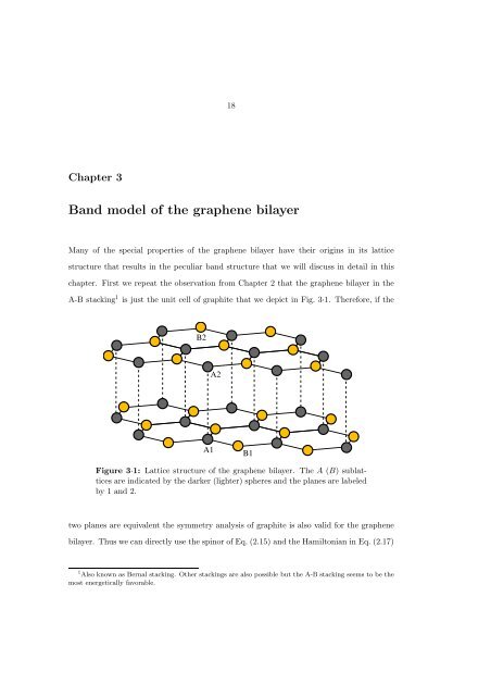
18Chapter 3<strong>Band</strong> <strong>model</strong> <strong>of</strong> <strong>the</strong> <strong>graphene</strong> <strong>bilayer</strong>Many <strong>of</strong> <strong>the</strong> special properties <strong>of</strong> <strong>the</strong> <strong>graphene</strong> <strong>bilayer</strong> have <strong>the</strong>ir origins in its latticestructure that results in <strong>the</strong> peculiar band structure that we willdiscussindetailinthischapter. First we repeat <strong>the</strong> observation from Chapter 2 that <strong>the</strong> <strong>graphene</strong> <strong>bilayer</strong> in <strong>the</strong>A-B stacking 1 is just <strong>the</strong> unit cell <strong>of</strong> graphite that we depict in Fig. 3·1. Therefore, if <strong>the</strong>B2A2A1B1Figure 3·1: Lattice structure <strong>of</strong> <strong>the</strong> <strong>graphene</strong> <strong>bilayer</strong>. The A (B) sublatticesare indicated by <strong>the</strong> darker (lighter) spheres and <strong>the</strong> planes are labeledby 1 and 2.two planes are equivalent <strong>the</strong> symmetry analysis <strong>of</strong> graphite is also valid for <strong>the</strong> <strong>graphene</strong><strong>bilayer</strong>. Thus we can directly use <strong>the</strong> spinor <strong>of</strong> Eq. (2.15) and <strong>the</strong> Hamiltonian in Eq. (2.17)1 Also known as Bernal stacking. O<strong>the</strong>r stackings are also possible but <strong>the</strong> A-B stacking seems to be <strong>the</strong>most energetically favorable.
19with Γ = 1 and γ 2 = γ 5 =0,leadingto:⎛⎞∆ v F pe iφ t ⊥ −v 4 v F pe −iφv F pe −iφ 0 −v 4 v F pe −iφ v 3 v F pe iφH 0 (p) =. (3.1)⎜ t ⊥ −v 4 v F pe iφ ∆ v F pe −iφ⎟⎝⎠−v 4 v F pe iφ v 3 v F pe −iφ v F pe iφ 0Ano<strong>the</strong>r way <strong>of</strong> arriving at Eq. (3.1) is to use <strong>the</strong> tight-binding <strong>model</strong> directly in <strong>the</strong> <strong>bilayer</strong>.Since <strong>the</strong> system is two-dimensional only <strong>the</strong> relative position <strong>of</strong> <strong>the</strong> atoms projected onto <strong>the</strong> x-y-plane enters into <strong>the</strong> <strong>model</strong>. The projected position <strong>of</strong> <strong>the</strong> different atoms areshown in Fig. 3·2. Since <strong>the</strong> A atoms are sitting right on top <strong>of</strong> each o<strong>the</strong>r in <strong>the</strong> lattice, <strong>the</strong>B2B1A1A2Figure 3·2: The real space lattice structure <strong>of</strong> <strong>the</strong> <strong>graphene</strong> <strong>bilayer</strong> projectedonto <strong>the</strong> x-y plane showing <strong>the</strong> relative positions <strong>of</strong> <strong>the</strong> differentsublattices.hopping term between <strong>the</strong> A1 andA2 atomsarelocalinrealspaceandhenceaconstantthat we denote by t ⊥ in momentum space. Referring back to Section 2.1 we note that <strong>the</strong>hopping B1 → A1 [A1 → B1] gives rise to <strong>the</strong> factor ζ(k) [ζ ∗ (k)], with ζ(k) definedinEq. (2.6). Since <strong>the</strong> geometrical role <strong>of</strong> <strong>the</strong> A and B atoms are interchanged between plane1andplane2weimmediatelyfindthatinFourierspace<strong>the</strong>hopping A2 → B2 [B2 → A2]gives rise to <strong>the</strong> factor ζ(k) [ζ ∗ (k)]. Fur<strong>the</strong>rmore, <strong>the</strong> direction in <strong>the</strong> hopping B1 → B2
20(projected on to <strong>the</strong> x-y plane) is opposite to that <strong>of</strong> hopping B1 → A1. Thus we associateafactorv 3 ζ ∗ (k) to<strong>the</strong>hoppingB1→ B2, where <strong>the</strong> factor v 3 = γ 3 /γ 0 is needed because<strong>the</strong> hopping energy is γ 3 instead <strong>of</strong> γ 0 = t. Similarly, <strong>the</strong> direction <strong>of</strong> hopping B1 → A2(projected on to <strong>the</strong> x-y plane) is <strong>the</strong> same as B1 → A1 and <strong>the</strong>refore <strong>the</strong> term −v 4 ζ(k)goes with <strong>the</strong> hopping B1 → A2. 2 Continuing to fill in all <strong>the</strong> entries <strong>of</strong> <strong>the</strong> matrix <strong>the</strong> fulltight-binding Hamiltonian in <strong>the</strong> <strong>graphene</strong> <strong>bilayer</strong> becomes:⎛⎞∆ ζ(k) t ⊥ −v 4 ζ ∗ (k)ζ ∗ (k) 0 −v 4 ζ ∗ (k) v 3 ζ(k)H t.b. (k) =, (3.2)⎜ t ⊥ −v 4 ζ(k) ∆ ζ ∗ (k)⎟⎝⎠−v 4 ζ(k) v 3 ζ ∗ (k) ζ(k) 0where ∆ parametrizes <strong>the</strong> difference in energy between <strong>the</strong> A and B atoms. We come backto Eq. (3.1) upon expanding this expression close to <strong>the</strong> K point. The typical behavior <strong>of</strong><strong>the</strong> bands obtained from Eq. (3.1) is shown in Fig. 3·3. Two <strong>of</strong> <strong>the</strong> bands (labeled 3 and4in<strong>the</strong>figure)aremovedawayfrom<strong>the</strong>Diracpointbyanenergythat is given by <strong>the</strong>interplane hopping term t ⊥ .E31tkFigure 3·3: <strong>Band</strong> dispersions near <strong>the</strong> K-points in <strong>the</strong> <strong>bilayer</strong>. <strong>Band</strong>s arelabeled by <strong>the</strong> numbers 1 − 4asin<strong>the</strong>text.242 The minus sign in front <strong>of</strong> v 4 follows from <strong>the</strong> conventional definition <strong>of</strong> γ 4 (Partoens and Peeters, 2006).
213.1 Simplified <strong>model</strong>Asimplified<strong>model</strong>thatonlyconsiders<strong>the</strong>interplanehoppingtermbetweenA atoms employsa matrix <strong>of</strong> <strong>the</strong> form⎛⎞0 v F pe iφ(p) t ⊥ 0v F pe −iφ(p) 0 0 0H 0 (p) =. (3.3)⎜ t ⊥ 0 0 v F pe −iφ(p)⎟⎝⎠0 0 v F pe iφ(p) 0From now on in this section, we use units such that v F =1asdiscussedinSection2.1. ThisHamiltonian has <strong>the</strong> advantage that it allows for relatively simple calculations. Some <strong>of</strong> <strong>the</strong>fine details <strong>of</strong> <strong>the</strong> physics might not be accurate but it will work as a minimal <strong>model</strong> andcapture most <strong>of</strong> <strong>the</strong> important physics. It is important to know <strong>the</strong>qualitativenature<strong>of</strong><strong>the</strong>terms that are neglected in this approximation, this will be discussed later in this Chapter.It is also an interesting toy <strong>model</strong> as it allows for (approximately) “chiral” particles withmass (i.e., a parabolic spectrum) at low energies as we will discuss in <strong>the</strong> next Section. Foralargepart<strong>of</strong>this<strong>the</strong>siswewillstudy<strong>the</strong>properties<strong>of</strong><strong>the</strong>system with this simplifiedHamiltonian.3.2 Approximate effective two-band <strong>model</strong>sThere are two main reasons for constructing approximate two-band <strong>model</strong>s:First, onphysical grounds <strong>the</strong> high-energy bands (far away from <strong>the</strong> Dirac point) should not be veryimportant for <strong>the</strong> low-energy properties <strong>of</strong> <strong>the</strong> system. Second, it is <strong>of</strong>ten easier to workwith 2 × 2matricesinstead<strong>of</strong>4× 4matrices. Inthissection,wederive<strong>the</strong>low-energyeffective <strong>model</strong> by doing degenerate second order perturbation <strong>the</strong>ory. The quality <strong>of</strong> <strong>the</strong>expansion is good as long as v F p ≪ t ⊥ ≈ 0.35 eV. We first present <strong>the</strong> general expressionfor <strong>the</strong> second-order 2 × 2effectiveHamiltonian,<strong>the</strong>reaftervarioussimplifiedformswillbeintroduced. Analyses similar to <strong>the</strong> one presented here were presented in (McCann andFal’ko, 2006) and (Nilsson et al., 2006c).
22Derivation <strong>of</strong> effective <strong>model</strong>sFirst we decompose Eq. (3.1) into a high-energy part K 0 and two low-energy parts K 1 andK 2 according to H 0 = K 0 + K 1 + K 2 ,with⎛⎞∆ 0 t ⊥ 00 0 0 0K 0 =, (3.4)⎜t ⊥ 0 ∆ 0⎟⎝⎠0 0 0 0⎛⎞0 pe iφ 0 −v 4 pe −iφpe −iφ 0 −v 4 pe −iφ 0K 1 = v F , (3.5)⎜ 0 −v 4 pe iφ 0 pe −iφ⎟⎝⎠−v 4 pe iφ 0 pe iφ 0⎛⎞0 0 0 00 0 0 v 3 pe iφK 2 = v F . (3.6)⎜0 0 0 0⎟⎝⎠0 v 3 pe −iφ 0 0The usual manipulations (Sakurai, 1994) <strong>the</strong>n given <strong>the</strong> Hamiltonian matrix in <strong>the</strong> lowenergy subspace as K low = K 2 −K † 1 P 1(1/K 0 )P 1 K 1 ,whereP 1 is <strong>the</strong> projection out <strong>of</strong> <strong>the</strong>low-energy subspace (explicitly P 1 =Diag[1, 0, 1, 0]). The result is:⎛⎞0 0 0 0K low =v2 F p20 2t ⊥ v 4 +∆(1+v4 2t 2 ⊥ − ) 0 −[ t ⊥ (1 + v4 2)+2v 4∆ ] e −2iφ+ K ∆2 ⎜0 0 0 02 ,⎟⎝0 − [ t ⊥ (1 + v4 2)+2v 4∆ ] ⎠e 2iφ 0 2t ⊥ v 4 +∆(1+v4 2) (3.7)
23and because this is really just a 2 × 2matrixin<strong>the</strong>low-energysubspacewecanwriteitas:H eff =⎛ ⎞{ v2 F p2 [2t⊥t 2 ⊥ − v 4 +∆(1+v 2∆2 4 )] ⎝ 1 0 ⎠0 1⎛− [ t ⊥ (1 + v4)+2v 2 4 ∆ ] ⎝ 0The corresponding eigenvalues are:E eff,± ≈v2 F p2 [t 2 ⊥ − 2t⊥ v 4 +∆(1+v4) 2 ]∆2√{ v2± (v 3 v F p) 2 + Fp 2[ t ⊥ (1 + v4 2)+2v 4∆ ]e−i2φe i2φ 0⎞ ⎛ ⎞}⎠ + v 3 v F p ⎝ 0 eiφ⎠ . (3.8)e −iφ 0} 2 2v 3 v −F 3 p3[ t ⊥ (1 + v4 2)+2v 4∆ ]t 2 ⊥ − ∆2 t 2 ⊥ − ∆2cos(3φ).(3.9)This expression shows that v 4 and ∆ weakly breaks <strong>the</strong> particle-hole symmetry <strong>of</strong> <strong>the</strong>system and that v 3 is responsible for breaking <strong>the</strong> cylindrical symmetry and <strong>the</strong> so-called“trigonal warping” <strong>of</strong> <strong>the</strong> energy bands.A simplified <strong>model</strong> that takes only <strong>the</strong> termsinvolving t ⊥ and <strong>the</strong> trigonal warping v 3 into account isH eff = − v2 F p2t ⊥⎛⎝ 0e−i2φe i2φ 0⎞ ⎛ ⎞⎠ + v 3 v F p ⎝ 0 eiφ⎠ . (3.10)e −iφ 0An even simpler <strong>model</strong> which neglects both <strong>the</strong> electron-hole asymmetry and <strong>the</strong> trigonalwarping is:H eff = − v2 F p2t ⊥⎛⎝ 0e−i2φe i2φ 0⎞⎠ . (3.11)This form is interesting since it gives rise to massive “chiral” quasi-particles (McCann andFal’ko, 2006). Here “chirality” means that <strong>the</strong>re exist an operator Ĉ defined by⎛Ĉ≡−⎝ 0e i2φ 0e−i2φ⎞⎠ , (3.12)
24that has <strong>the</strong> eigenvalues ±1 andcommuteswith<strong>the</strong>Hamiltonian. Thisimpliesthat<strong>the</strong>reis ano<strong>the</strong>r quantum number (in addition to <strong>the</strong> energy) with which one can label <strong>the</strong> states<strong>of</strong> <strong>the</strong> system.3.3 <strong>Band</strong> structure comparisonsAcomparison<strong>of</strong><strong>the</strong>bandsobtainedfrom<strong>the</strong>simpleHamiltonian in Eq. (3.3) and thoseobtained from <strong>the</strong> full Hamiltonian in Eq. (3.1) on a large scale is shown in Fig. 3·4. Thisfigure clearly shows that <strong>the</strong> gross features <strong>of</strong> <strong>the</strong> bands are correctly captured in <strong>the</strong> simpleminimal <strong>model</strong>.0.40.40.20.2EeV0-0.2EeV0-0.2-0.4-0.4-0.2 -0.1 0 0.1 0.2k eV(a)-0.2 -0.1 0 0.1 0.2k eV(b)Figure 3·4: Comparison between <strong>the</strong> bands obtained from <strong>the</strong> full Hamiltonianin Eq. (3.1) and those <strong>of</strong> <strong>the</strong> simple minimal <strong>model</strong> in Eq. (3.3)along<strong>the</strong> direction φ =0in<strong>the</strong>BZ.(a)FullHamiltonian. (b)Minimal<strong>model</strong>Hamiltonian.That <strong>the</strong> low-energy effective <strong>the</strong>ory in Eq. (3.8) and Eq. (3.9) is accurate for lowenergies is shown in Fig. 3·5. But as one moves away from <strong>the</strong> Dirac point deviations from<strong>the</strong> real spectrum is clearly visible.We show, in Figure 3·6 andinFigure3·7, a comparison <strong>of</strong> <strong>the</strong> bands obtained from <strong>the</strong>simple minimal Hamiltonian in Eq. (3.3) and those <strong>of</strong> <strong>the</strong> full Hamiltonian in Eq. (3.1) forlow energies. This shows that especially γ 3 ,whichgivesriseto<strong>the</strong>“trigonaldistortion”,significantly changes <strong>the</strong> behavior at <strong>the</strong> lowest energies. A normal Dirac cone is found atp =0at<strong>the</strong>lowestenergies,butnow<strong>the</strong>Fermi-Diracvelocityis v 3 v F . There is also <strong>the</strong>
25EeV0.040.030.020.010-0.1 -0.05 0 0.05 0.1k eV(a)EeV0.0080.0060.0040.0020-0.04 -0.02 0 0.02 0.04k eV(b)Figure 3·5: Comparison between <strong>the</strong> bands obtained from <strong>the</strong> full Hamiltonianin Eq. (3.1) and those <strong>of</strong> <strong>the</strong> effective <strong>model</strong> in Eq. (3.8) alongdifferentdirections in <strong>the</strong> BZ. Solid line – [φ =0,Eq.(3.1)],Dash-dottedline–[φ =0,Eq.(3.8)],Dashedline–[φ = π/6, Eq. (3.1)], Dotted line –[φ = π/6, Eq. (3.8)]. (a) Larger energy scale. (b) Zoom in at low energies.extra band crossings in <strong>the</strong> directions φ =0andφ = ±2π/3 whichgivesrisetoellipticalDirac cone 3 away from <strong>the</strong> point p =0. Thisstructureispresentatasmallenergyscale<strong>of</strong><strong>the</strong> order <strong>of</strong> ∼ 1meV, <strong>the</strong>refore experimental probes that are sensitive to this energy scaleare necessary to be able to detect <strong>the</strong>se features. Moreover, as we will see in Chapter 5,different forms <strong>of</strong> disorder can easily generate energies <strong>of</strong> this scale or larger in <strong>the</strong> realexperimental samples, thus this structure might be hard to detect experimentally.Astudy<strong>of</strong>few-layer<strong>graphene</strong>systems(including<strong>graphene</strong><strong>bilayer</strong>s) with plots similarto those in this chapter can be found in (Partoens and Peeters, 2006). Afirst-principlesstudy with both similar scope and results also exists (Latil and Henrard, 2006).3 This means that <strong>the</strong>re are two inequivalent perpendicular axes (1 and 2) in <strong>the</strong> cone, with two differentvalues <strong>of</strong> <strong>the</strong> Fermi velocity v F1 ≠ v F2. Thespectrumis<strong>the</strong>n± p v 2 F1 p2 1 + v2 F2 p2 2 .
26EeV0.020.010-0.01-0.02-0.1 -0.05 0 0.05 0.1k eV(a)EeV0.0030.0020.0010-0.001-0.002-0.04 -0.02 0 0.02 0.04k eV(b)Figure 3·6: Comparison between <strong>the</strong> low-energy bands obtained from <strong>the</strong>simple <strong>model</strong> in Eq. (3.3): solid lines; and those <strong>of</strong> <strong>the</strong> full Hamiltonian inEq. (3.1) along three different directions in <strong>the</strong> BZ: φ =0(dashed),φ = π/9(dashed-dotted), and φ =2π/9 (dotted). (a)Largerenergyscale. (b)Zoomin at low energies.k y meV6040200-20-40-60k y meV6040200-20-40-60-60 -40 -20 0 20 40 60k x meV(a)-60 -40 -20 0 20 40 60k x meV(b)Figure 3·7: Comparison between <strong>the</strong> bands obtained from <strong>the</strong> full Hamiltonianand those <strong>of</strong> <strong>the</strong> simple minimal <strong>model</strong> at low energies using a contourplot: (a) Full Hamiltonian (b) Simplified Hamiltonian. The contours are at<strong>the</strong> energies: 0.1, 0.3, 0.5, 1, 2, 3, 4meV(black lines, orderedfrom <strong>the</strong>solidline to <strong>the</strong> more dotted), 5, 10, 20 meV (gray lines, same ordering).