7 CHI-SQUARED GOODNESS OF FIT TEST FOR GENERALIZED BIRNBAUM ...

M. S. Nikulin and X. Q. Tran – CHI-SQUARED GOODNESS-OF-FIT TETS FOR GENERALIZED BIRNBAUM-SAUNDERS MODELS FORRIGHT CENSORED DATA AND ITS RELIABILITY APPLICATIONSRT&A # 02 (29)(Vol.8) 2013, JuneDistribution Notation c g(z ), z ∈ RPearson VIIKotz typePVII(q, r)KT(q, r, s)() √1 + , q > , ν > 0 () ⁄ z () e , q > , r > 0, s > 0Table 1: Kernel g(∙) and normalization constants c for some indicated distributions.Following Díaz-García et al. the random variable T in (1) allows the GBS distributions,denoted by T ≈ GBS(α, β ; g),T = β α z 4 + α z 2 + 1 ≈ GBS(α, β, g), α > 0, β > 0,iff the random variable Z which is given by the expressionZ = − ≈ EC(0, 1; g).So, the probability density function of T can be written asf (t, α, β) = + g − , t > 0, α > 0, β > 0, (3)the cumulative distribution function of T ≈ GBS(α, β ; g) is expressed byF (t, α, β) = F , t > 0, α > 0, β > 0, (4)the GBS hazard rate, survival and cumulative hazard functions areλ (t, α, β) = f a (α, β)A (α, β)1 − F a (α, β) ,S (t, α, β) = 1 − F a (α, β) , and Λ (t, α, β) = −ln{S (t, α, β)},(5)respectively, wherea (α, β) = − ; A (α, β) = + . It is clear that the properties of GBS distributions depends on the kernel function g(∙) and theunknown parameter θ = (α, β) . The statistical theory and methodology of the GBS distributions,also some results for this flexible family of distributions mainly related to transformations, thehazard failure and censored data type II which can be found in the works of Sanhueza, Leiva etal.[36].Table 2 below shown some probability density function of T ≈ GBS(α, β ; g),corresponding the specific symmetric distribution EC(0, 1; g) in Table 1.The Figure 1, 2, 3 and 4 below illustrates some curve of the probability densities and hazardrate functions of T ≈ GBS(α, β ; g), allows with the kernel indicative.Kernel g(∙)N(0, 1)DistributionGBS-Normal(BS)Probability density function of T ≈ GBS(α, β ; g),f(t, α, β; g), (t > 0, α > 0, β > 0)1 31 2 2 1 t exp 2222t t t 9

M. S. Nikulin and X. Q. Tran – CHI-SQUARED GOODNESS-OF-FIT TETS FOR GENERALIZED BIRNBAUM-SAUNDERS MODELS FORRIGHT CENSORED DATA AND ITS RELIABILITY APPLICATIONSRT&A # 02 (29)(Vol.8) 2013, JuneKernelDistributionProbability density function of ,GBS-StudentL(0, 1) GBS-LaplaceLog(0, 1) GBS-LogisticC(0, 1) GBS-CauchyKT(q, r, s) GBS-KTPVII(q, r) GBS-PVIIPE(r, s) GBS-PETable 2: The p.d.f of11 3 22 2 1 t 1 222 ( 2) t t t 1 3 2 2 1 1 t exp 4 t t t 1 t 1 3exp 1 2 2 t 2 t t 1 t 1 exp t 1 1 t 1 222 t t t 1 3 12 21 32 22q1 2s2q3sr t t r t1q 2s s exp 2 2q1 t2 t 2s 2 t 2( 1)21 3 ( q) 2 2 1 t 1 222 r( q 1/ 2) t t t 1 1 3 2s2s2 2 sr r t exp2s1 2 ( )t t t 2sfor some indicated distributions. 12Figure 1: Plots of densities for given kernel .10

M. S. Nikulin and X. Q. Tran – CHI-SQUARED GOODNESS-OF-FIT TETS FOR GENERALIZED BIRNBAUM-SAUNDERS MODELS FORRIGHT CENSORED DATA AND ITS RELIABILITY APPLICATIONSRT&A # 02 (29)(Vol.8) 2013, JuneFigure 2: Plots of densities for given kernel .Figure 3: Plots of failures rates for given kernel .Figure 4: Plots of failures rates for given kernel .3 Chi-squared type tests for right censored dataFollowing Bagdonavičius and Nikulin ([3], [4]), we describe a chi-squared test for testingcomposite parametric hypothesis when data are right censored.Suppose thatare failures time non-negative and independent and the probabilitydensity function of the random variable belong to a parametric family .The censoring variablesare also non-negative and assumed to be random sample. Letus and are independent. We observed(6)where,11

M. S. Nikulin and X. Q. Tran – CHI-SQUARED GOODNESS-OF-FIT TETS FOR GENERALIZED BIRNBAUM-SAUNDERS MODELS FORRIGHT CENSORED DATA AND ITS RELIABILITY APPLICATIONSRT&A # 02 (29)(Vol.8) 2013, JuneX = T ∧ C ,δ = 1 { }, i = 1, 2, ⋯ , n.Defined thatf(t, θ)S(t, θ) = P θ (T > t); λ(t, θ) =S(t, θ) , Λ(t, θ) = − ln{S(t, θ)} , θ ∈ Θ ⊆ R ,be the survival, hazard rate and cumulative hazard functions, respectively. Denote by G and g arethe survival and the density function of the censoring time C , respectively. Supposing that the rightcensoring is non-informative which means that the function G does not depend on θ. So in thiscase, we obtain the following expressions for the likelihood function L(θ)L(θ) = f (X , θ)S (X , θ)g (C )G (C ).So the members with G and g do not contain θ, so they can be rejected. The likelihoodfunction is obtainedL(θ) = f (X , θ)S (X , θ) = λ (X , θ)S(X , θ) . (7)The estimator θ maximizing the likelihood function L(θ). The log-likelihood function isl(θ) = {δ ln λ(X , θ) + ln S(X , θ)}= {δ ln λ(X , θ) − Λ(X , θ)}.The maximum likelihood estimator θ satisfies the system equationsl̇θ = 0 ,where l̇(θ) are the score vectorswherel̇(θ) = l(θ) = l(θ) The Fisher information matrix is defined asI(θ) = −E l̈(θ),l̈(θ) = δ ∂ ∂θ ln λ(X , θ), l(θ), ⋯ , l(θ) . − ∂∂θ Λ(X , θ) .Supposing that θ is the true value of θ, under some regularity conditions, we haveθ → θ ; √n θ − θ = i (θ ) 1√n l̇(θ ) + O (1) , −1√n l̈θ → i(θ ),√n(θ − θ ) → 1N (0, i (θ ));√n l̇(θ ) → N (0, i(θ )),where, θ are the maximum likelihood estimation of θ and the matrixI(θi(θ ) )= lim → n .For any t ≥ 0, setN (t) = 1 { , } = 1, if t ≥ X and δ = 1,; Y0, if 0 ≤ t ≤ X . (t) = 1 { } = 1, if t ≤ X ,0, if t > X .N(t) = N (t) , Y(t) = Y (t).The process N(t) shows the number of observed failures in the interval [0, t] and the processY(t) shows the number of objects which are "at risk" just prior to time t. The sample (6) isequivalent to the sample (8)12

M. S. Nikulin and X. Q. Tran – CHI-SQUARED GOODNESS-OF-FIT TETS FOR GENERALIZED BIRNBAUM-SAUNDERS MODELS FORRIGHT CENSORED DATA AND ITS RELIABILITY APPLICATIONSRT&A # 02 (29)(Vol.8) 2013, June(N (t), Y (t), t ≥ 0), (N (t), Y (t), t ≥ 0), ⋯ , (N (t), Y (t), t ≥ 0). (9)For the sample (9), the parametric log-likelihood function can be written by expression followsl(θ) = ∫ {ln λ(u, θ) dN(u) − Y(u)λ(u, θ)}du.The score function isandl̇(θ) = ∂ ln λ(u, θ) {dN(u) − Y(u)λ(u, θ)du} = ∂ ln λ(u, θ) dM(u, θ) ,∂θ ∂θl̈(θ) = ∂∂θ ln λ(u, θ)dM (u, θ) − ∂∂θ ln λ(u, θ) ∂∂θ ln λ(u, θ) λ(u, θ)Y (u)du ,where, M (t, θ) = N (t) − ∫ Y (u)λ(u, θ)du , (θ ∈ Θ) is the zero mean martingale with respectto the filtration generated by the data.Suppose that the processes N and Y are observed for finite time τ > 0, which means that attime τ, observation on all surviving objects are censored, and so instead of using censoring time C .In this case, the matrix Fisher information can be written asI(θ) = −E θ l̈(θ) = E ∂∂ln λ(u, θ) ∂θ ∂θ ln λ(u, θ) λ(u, θ)Y (u)du. Let be consider next the hypothesisH ∶ F(x) ∈ F = {F (x, θ), θ ∈ Θ ⊆ R },here, θ = (θ , θ , ⋯ , θ ) are an unknown m-dimensional parameters and F is a knowndistribution function.Subdividing the interval [0, τ] into k > m smaller intervals I = a , a , with a = 0,a = τ, and denote byU = Na − Na ,the number of observed failures in the j interval I , ( j = 1, 2, ⋯ , k ). Let e = λu, θ Y(u)du .A chi-squared test which was proposed by Bagdonavičius and Nikulin [21], based on the vectorZ = (Z , Z , ⋯ , Z ) 1, with Z =√n U − e , j = 1, 2, ⋯ , k. (10)Under the conditions1) There exists a neighborhood Θ of θ such that for all n and θ ∈ Θ , and almost allt ∈ [0, τ], the partial derivatives of λ(t, θ) of the first, second and third order with respect to θexist and are continuous in θ for θ ∈ Θ . Moreover, they are bound in [0, τ] × Θ and the loglikelihoodfunction may be differentiated three times with respect to θ ∈ Θ , by interchanging theorder of integration and differentiation.2) λ(t, θ) is bound away from zero in [0, τ] × Θ .3) A positive deterministic function y(t) exists such that sup ∈[,] ()− y(t) → 0.(θ4) Under condition 1) - 3), the matrix i(θ ) = lim ) → is positive definite.The statistic of Bagdonavičius and Nikulin given as13

M. S. Nikulin and X. Q. Tran – CHI-SQUARED GOODNESS-OF-FIT TETS FOR GENERALIZED BIRNBAUM-SAUNDERS MODELS FORRIGHT CENSORED DATA AND ITS RELIABILITY APPLICATIONSRT&A # 02 (29)(Vol.8) 2013, JuneY (θ ) = Z Σ Z, (11)where, Σ is the general inverse matrix of the covariance matrix Σ,Σ = A − C I C,Σ = A + A C G CA , G = I − CA C ,A is the diagonal k × k matrix with the elements A = on the diagonal, A is inverse matrixof A, andC = [C ] × , with C = ∑ δ ( ,): ∈ , l = 1, 2, ⋯ , m, j = 1, 2, ⋯ , k, (13)I = [ı̂ ] × , with ı̂ = 1 n δ where, ∂ ln λ(X , θ)∂θ ∂ ln λ(X , θ)∂θ (12), l, l = 1, 2, ⋯ , m. (14)From the definition of Z in (10), the test statistic Y (θ ) should be written asY θ = X + Q, (15)X = (U − e ) U , Q = W G W , W = CA Z, G = I − CA C .Under the hypothesis H , the limiting distribution of the statistics Y θ is chi-squared withr = rank(Σ ) degrees of freedom that is,lim → PY θ > x | H = P{χ > x}, for any x > 0.Statistical inference for the hypothesis H 0 : The null hypothesis H is rejected with approximatesignificance level α if Y θ > χ (r) or Y θ < χ (r) depending on an alternative, whereχ (r) and χ (r)corresponding are the upper and lower α percentage points of the χ distribution, respectively.Using the method of interval selection which is proposed by Bagdonavičius, and Nikulin [20],we used a as the random data function. DefineE = ∑ Λ(X , θ ) , E = E , j = 1, 2, ⋯ , k.Denote by X () , X () , ⋯ , X () the ordered sample from X , X , ⋯ , X . Setb = (n − i)ΛX () , θ + ΛX () , θ , i = 1, 2, ⋯ , n,if i is the smallest natural number verifying b ≤ E ≤ b then a verifying the equality(n − i + 1)Λa , θ + ΛX () , θ = E Soa = Λ E − ∑ Λ(X () , θ ), θn − i + 1 ; a = maxX () , τ , (j = 1, 2, ⋯ , k − 1). (16)where Λ is the inverse of the function Λ. We have: 0 < a < a < ⋯ < a , with this choiceof intervals, then e = , for all j.Application for GBS distributions: In particular, we shall give chi-squared tests NRR forthe hypothesis H that the data X are coming from the GBS distributions with the probability14

M. S. Nikulin and X. Q. Tran – CHI-SQUARED GOODNESS-OF-FIT TETS FOR GENERALIZED BIRNBAUM-SAUNDERS MODELS FORRIGHT CENSORED DATA AND ITS RELIABILITY APPLICATIONSRT&A # 02 (29)(Vol.8) 2013, Junedensity, cumulative distribution, hazard rate, survival and cumulative hazard functions give informulas (3), (4) and (5), respectively.The GBS log-likelihood functions l(θ), (θ = (α, β) ) isl(θ) = −δ ln α − δ ln β + δ ln β β + X X + δ ln{1 − F (a (α, β))}15+ δ lngK (α, β)Let θ = α, β be maximum likelihood estimations which are solutions of the non-linearsystem equationsl̇ (θ), l̇ (θ) = 0 .Using the formula (13) – (14), the elements ı̂ , (l, l = 1, 2) of the Fisher information matrixI = [ı̂ ] × are1ı̂ =nα δ −1 + K α, βv K α, β − A (α, β)f (A (α, β))1 − F (A (α, β)) ,ı̂ =ı̂ =1nβ δ −1 + 1 21 + 3 1 + + 1 2 A α, βB α, βv K α, β − 1 21nαβ δ −1 + K α, βv K α, β − A (α, β)f (A (α, β))1 − F (A (α, β)) ×× −1 + 1 1 + 3 2 1 + + 1 2 A α, βB α, βv K α, β − 1 2 and the matrix C = C ×given by1C =C =where,nα δ −1 + K α, βv K α, β − A (α, β)f (A (α, β))1 − F (A (α, β)) B (α, β)f (A (α, β))1 − F (A (α, β)) ,∶ ∈ ,B (α, β)f (A (α, β))1 − F (A (α, β)) ,1 δ −1 + 1 1 + 3 nβ2 1 + + 1 2 A α, βB α, βv K α, β − 1 B (α, β)f (A (α, β))2 1 − F (A (α, β)) .∶ ∈ A α, β = 1 α X β − β ,X B α, β = 1 α X β + β ,X K α, β = 1 α X β + β − 2 , i = 1, 2, ⋯ , n.X and f (u) = c g(u ), F (∙) are the probability density function and cumulative function of therandom variable Z ≈ EC(0, 1; g) which follows a standard symmetrical distribution in R with thekernel g(∙), respectively, andv(u) = −2w(u); w(u) = g (u), u > 0,g(u)are the transformations functions of kernel function g(u), and w (u) is the derivative of w(u)([15], [16]). Table 3 below shown some transformations functions w(u) and its derivativew (u), (u > 0) corresponding with kernel g(u) of indicated Elliptic distributions EC(0, 1; g).

M. S. Nikulin and X. Q. Tran – CHI-SQUARED GOODNESS-OF-FIT TETS FOR GENERALIZED BIRNBAUM-SAUNDERS MODELS FORRIGHT CENSORED DATA AND ITS RELIABILITY APPLICATIONSRT&A # 02 (29)(Vol.8) 2013, Junew(u)w (u)N(0, 1) t(ν) L(0, 1) Log(0, 1) PE(ν)−120− ν + 12(ν + u)− 12√uν + 112(ν + u) 4u√u− 1 tanh √u2√u 2 − ν 2 usinh √u − √u4u√u[1 + cosh √u]−ν[ν − 1]u 2Table 3: Transformations functions w(u) and its derivative w’(u), (u > 0) for kernel g(u) of theindicated Elliptic distributions EC(0, 1; g).Chi-squared test for GBS distributions: Under the hypothesis H , the matrix G is nondegenerate.So, the hypothesis H is rejected with approximate significance level α ifY θ > χ (α).It is necessary to note that: PE(ν) ≅ KT(1, 0.5, ν), N(0, 1) ≅ KT(1, 0.5, 1), L(0, 1) ≅PE(0.5), t(ν) ≅ PVII([ν + 1] ⁄ 2 , ν), Log(0, 1) ≅ LIII(1).Thus, the next section, we consider goodness of fit test for following five distributions: GBS-N(0, 1) which known as BS distribution, GBS-Laplace, GBS-Logistic, GBS-t(ν) and GBS-Cauchy distributions.4 Real studyAll distributions presented in the next two examples by using R statistics software, weanalyze the goodness of fit test for the parametric generalized BS distributions in two studies to adata of breast cancer which set from research of Boag (1949) and the data from a laboratoryinvestigation in which the vaginas of rats were painted with the carcinogen DMBA of Pike (1966).4.1 Analysis of breast cancer dataBoag [10] was presented the survival times for 121 patients treated for cancer of the breast inone particular hospital during the years 1929-1938 which given in table below. The times are inmonths, and asterisks denote censoring times. This data included 66 observations and 55 censoringtimes.0.3 7.4 ∗ 13.5 16.8 21.0 29.1 37 ∗ 41 45 ∗ 52 60 ∗ 78 105 ∗129 ∗ 0.3 ∗ 7.5 14.4 17.2 21.1 30 38 41 46 ∗ 54 61 ∗ 80109 ∗ 129 ∗ 4.0 ∗ 8.4 14.4 17.3 23.0 31 38 ∗ 41 ∗ 46 ∗ 55 ∗ 62 ∗83 ∗ 109 ∗ 139 ∗ 4.0 ∗ 8.4 14.4 17.3 23.0 31 38 ∗ 41 ∗ 46 ∗ 55 ∗ 62 ∗83 ∗ 109 ∗ 139 ∗ 5.0 8.4 14.8 17.5 23.4 ∗ 31 38 ∗ 42 47 ∗ 5665 ∗ 88 ∗ 111 ∗ 154 ∗ 5.6 10.3 15.5 ∗ 17.9 23.6 32 39 ∗ 43 ∗ 4857 ∗ 65 ∗ 89 115 ∗ 6.2 11.0 15.7 19.8 24.0 35 39 ∗ 43 ∗ 49 ∗58 ∗ 67 ∗ 90 117 ∗ 6.3 11.8 16.2 20.4 24.0 35 40 43 ∗ 5159 ∗ 67 ∗ 93 ∗ 125 ∗ 6.6 12.2 16.3 20.9 27.9 37 ∗ 40 ∗ 44 5160 68 ∗ 96 ∗ 126 6.8 12.3 16.5 21.0 28.2 37 ∗ 40 ∗ 45 ∗ 51 ∗60 ∗ 69 ∗ 103 ∗ 127 ∗Firstly, we consider the hypothesis H that the survival times for 121 breast cancer patientsbelongs the Birnbaum-Saunders distribution. In this case, MLE’s of the parameters θ = (α, β) ofthe BS distribution are θ = (2.04798, 47.11415) .Choosing the sub-intervals k = 6. The values of a , the frequency vector Z and the elementsof the matrix C give in table follows.16

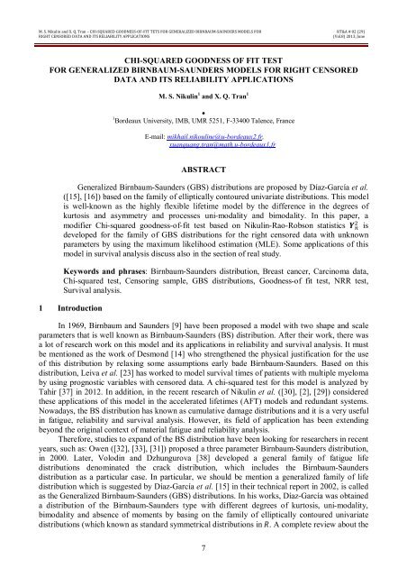
M. S. Nikulin and X. Q. Tran – CHI-SQUARED GOODNESS-OF-FIT TETS FOR GENERALIZED BIRNBAUM-SAUNDERS MODELS FORRIGHT CENSORED DATA AND ITS RELIABILITY APPLICATIONSRT&A # 02 (29)(Vol.8) 2013, JuneFigure 5: GBS with indicated kernel, Weibulland Kaplan-Meier estimate of for dataof Boag (1949).Figure 6: GBS with indicated kernel andKaplan-Meier estimate of for the dataof Pike (1966).We consider next the hypotheses that the data above follows the GBS distributions in thecases of kernel : Standard Normal distribution , Standard Logistic distribution ,Standard Cauchy distribution . Choosing grouping intervals , the results given in table5 below.Distribution-valueGBS- 3.125849 16.35656 19.48241 0.0006316GBS- 1.000369 2.885825 3.886194 0.4216269GBS- 0.749583 0.325662 1.075246 0.8981795GBS- 0.745397 0.3637746 1.109172 0.8928143Table 5: MLE’s of , values of and p-values with indicated kernel distributions,data of Pike (1966).We plot the estimated GBS survivor functionscorrespond indicated kerneland the Kaplan-Meier estimate for the data of Pike (1966) in Figure 6.In this example, it is clear that the data are the best in concord with GBS-Logistic, GBS-Cauchy and GBS- distributions, it also acceptes for two parameters Weibull distribution.However, these data contradict the BS distribution much very strongly.5 Summary and conclusionIn this paper, we have presented a modifier Chi-squared goodness-of-fit test for generalizedBirnbaum-Saunders distributions. The results obtained in our examples show that the consideredfamilies are in accordance with lifetimes data. In addition, its hazard rate functions can be unimodalor bimodal by adjusting the values of its parameters and its kernel . So, it is necessary touse it as a baseline hazard rate functions in the parametric survival model. We would like to thankour colleagues, PhD. R. Tahir and N. Saaidia for valuable comments, which helped us improve thepresentation.18

M. S. Nikulin and X. Q. Tran – CHI-SQUARED GOODNESS-OF-FIT TETS FOR GENERALIZED BIRNBAUM-SAUNDERS MODELS FOR RIGHT CENSOREDDATA AND ITS RELIABILITY APPLICATIONSRT&A # 01 (28)(Vol.8) 2013, MarchReferences[1] Anderson, T. W. and Fang, K. T. Statistical inference in elliptically contoured and relateddistributions, Allerton Press New York, 1990.[2] Bagdonavičius, V. B. and Nikulin, M. S. Statistical models to analyze failure, wear, fatigue,and degradation data with explanatory variables. Communications in Statistics—Theory andMethods, vol. 38, no. 16-17, pp. 3031-3047, 2009.[3] Bagdonavičius, V. B. and Nikulin, M. S. Chi-squared tests for general composite hypothesesfrom censored samples. Comptes Rendus Mathematique, vol. 349, no. 3, pp. 219-223, 2011.[4] Bagdonavičius, V. B. and Nikulin, M. S. Chi-squared goodness-of-fit test for right censoreddata. International Journal of Applied Mathematics and Statistics, vol. 24, no. SI-11A, pp.30-50, 2011.[5] Bagdonavičius, V. B., Krupois, J. and Nikulin, M. S. Non-parametric Tests for CensoredData, Wiley, 2011.[6] Bagdonavičius, V. B., Levuliene, R. J. and Nikulin, M. S. Exact goodness-of-fit tests forshape-scale families and type II censoring. Lifetime Data Analysis, pp. 1-23, 2012.[7] Bagdonavičius, V. B. and M. S. Nikulin, Statistical methods to analyse failures of complexsystems in presence of wear, fatigue and degradation: An engineering perspective inaccelerated trials. In Electronic Instrument Engineering, 2008. APEIE 2008. 9thInternational Conference on Actual Problems of, 2008.[8] Balakrishnan, N. Handbook of the logistic distribution, vol. 123, CRC Press, 1992.[9] Birnbaum, Z. W. and Saunders, S. C. A new family of life distributions. Journal of AppliedProbability, pp. 319-327, 1969.[10] Boag, J. W. Maximum likelihood estimates of the proportion of patients cured by cancertherapy. Journal of the Royal Statistical Society. Series B (Methodological), vol. 11, no. 1,pp. 15-53, 1949.[11] BolShev, L. N. and Mirvaliev, M. Chi Square Goodness-of-Fit Test for the Poisson,Binomial and Negative Binomial Distributions. Theory of Probability \& Its Applications,vol. 23, no. 3, pp. 461-474, 1979.[12] Cambanis, S., Huang, S. and Simons, G. On the theory of elliptically contoured distributions.Journal of Multivariate Analysis, vol. 11, no. 3, pp. 368-385, 1981.[13] Chernoff, H. and Lehmann, E. L. The use of maximum likelihood estimates in χ tests forgoodness of fit. The Annals of Mathematical Statistics, vol. 25, no. 3, pp. 579-586, 1954.[14] Desmond, A. Stochastic models of failure in random environments. Canadian Journal ofStatistics, vol. 13, no. 3, pp. 171-183, 1985.[15] Díaz-García, J. A. and Leiva-Sánchez, V. A new family of life distributions based onBirnbaum-Saunders distribution. Technical report I-02-17 (PE/CIMAT), Mexico. 2002.[16] Díaz-García, J. A. and Leiva-Sánchez, V. A new family of life distributions based on theelliptically contoured distributions. Journal of Statistical Planning and Inference, vol. 128,no. 2, pp. 445-457, 2005.[17] Drost, F. C. Asymptotics for generalized chi-square goodness-of-fit tests. CWI Tracts, vol.48, pp. 1-104, 1988.[18] Dzaparidze, K. O. and Nikulin, M. S. On a modification of the standard statistics of Pearson.Theory of Probability & Its Applications, vol. 19, no. 4, pp. 851-853, 1975.[19] Fang, K. T., Kotz S. and Kai Wang, Ng. Symmetric Multivariate and Related Distributions,Monographs on Statistics and Applied Probability. 36, London: Chapman and Hall Ltd.MR1071174, 1990.[20] Greenwood, P. E. and Nikulin, M. S. A guide to chi-squared testing. Wiley New York, 1996.[21] Gupta, A. K. and Varga, T. Elliptically contoured models in statistics. Kluwer AcademicPublishers, 1993.19

M. S. Nikulin and X. Q. Tran – CHI-SQUARED GOODNESS-OF-FIT TETS FOR GENERALIZED BIRNBAUM-SAUNDERS MODELS FOR RIGHT CENSOREDDATA AND ITS RELIABILITY APPLICATIONSRT&A # 01 (28)(Vol.8) 2013, March[22] LeCam, L., Mahan, C., and Singh, A. An extension of a theorem of H. Chernoff and ELLehmann. Recent advances in statistics, 303-332, 1983.[23] Leiva, V., Barros, M., and Galea, G. A. Influence diagnostics in log-Birnbaum--Saundersregression models with censored data. Computational Statistics & Data Analysis, vol. 51, no.12, pp. 5694-5707, 2007.[24] Leiva, V., Riquelme, M., Balakrishnan, N. and Sanhueza, A. Lifetime analysis based on thegeneralized Birnbaum-Saunders distribution. Computational Statistics & Data Analysis, vol.52, no. 4, pp. 2079-2097, 2008.[25] Lawless, J. F. Statistical models and methods for lifetime data. New Jersey: John Wiley andSons Publishers, 2003.[26] Nikulin, M. S. Chi-square test for normality. In Proceedings of International VilniusConference on Probability Theory and Mathematical Statistics, 1973a.[27] Nikulin, M. S. On a chi-square test for continuous distribution. Theory of Probability and itsApplication, vol. 19, pp. 638-639, 1973b.[28] Nikulin, M. S. Chi-square test for continuous distributions with location and scaleparameters. Teoriya Veroyatnostei i ee Primeneniya, vol. 18, no. 3, pp. 583-591, 1973c.[29] Nikulin, M. S., Saaidia, N. and Tahir, R. Reliability analysis of redundant systems bysimulation for data with unimodal hazard rate functions. Journal| MESA, vol. 2, no. 3, pp.277-286, 2011.[30] Nikulin, M. S., Saaidia, N. and Tahir, R. Recent Results in the Analysis of RedundantSystems. Recent Advances in System Reliability, pp. 181-193, 2012.[31] Owen, W. J. A new three-parameter extension to the Birnbaum-Saunders distribution.Reliability, IEEE Transactions on, vol. 55, no. 3, pp. 475-479, 2006.[32] Owen, W. J. and Padgett, W. J. A Birnbaum-Saunders accelerated life model. Reliability,IEEE Transactions on, vol. 49, no. 2, pp. 224-229, 2000.[33] Owen, W. J. and Padgett, W. J. Power-law Accelerated Birnbaum-Saunders life models.International Journal of Reliability, Quality and Safety Engineering, vol. 7, no. 01, pp. 1-15,2000.[34] Pike, M. C. A method of analysis of a certain class of experiments in carcinogenesis.Biometrics, vol. 22, no. 1, pp. 142-161, 1966.[35] Rao, K. C. and Robson, B. S. A chi-squabe statistic for goodies-of-fit tests within theexponential family. Communications in Statistics-Theory and Methods, vol. 3, no. 12, pp.1139-1153, 1974.[36] Sanhueza, A., Leiva, V. and Balakrishnan, N. The generalized Birnbaum–Saundersdistribution and its theory, methodology, and application. Communications in Statistics—Theory and Methods, vol. 37, no. 5, pp. 645-670, 2008.[37] Tahir, R. On Validation Of Parametric Models Applied In Survival Analysis And Reliabilty.Thesis of University Bordeaux I, 2012.[38] Volodin, I. N. and Dzhungurova, O. A. On limit distributions emerging in the generalizedBirnbaum-Saunders model. Journal of Mathematical Sciences, vol. 99, no. 3, pp. 1348-1366,2000.20