7 CHI-SQUARED GOODNESS OF FIT TEST FOR GENERALIZED BIRNBAUM ...

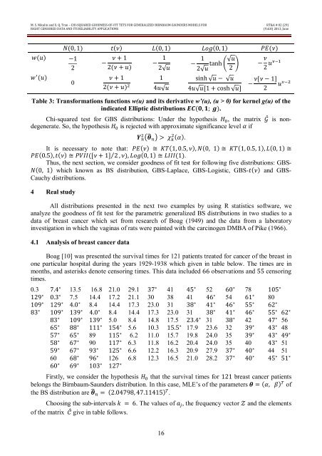
M. S. Nikulin and X. Q. Tran – CHI-SQUARED GOODNESS-OF-FIT TETS FOR GENERALIZED BIRNBAUM-SAUNDERS MODELS FORRIGHT CENSORED DATA AND ITS RELIABILITY APPLICATIONSRT&A # 02 (29)(Vol.8) 2013, Junew(u)w (u)N(0, 1) t(ν) L(0, 1) Log(0, 1) PE(ν)−120− ν + 12(ν + u)− 12√uν + 112(ν + u) 4u√u− 1 tanh √u2√u 2 − ν 2 usinh √u − √u4u√u[1 + cosh √u]−ν[ν − 1]u 2Table 3: Transformations functions w(u) and its derivative w’(u), (u > 0) for kernel g(u) of theindicated Elliptic distributions EC(0, 1; g).Chi-squared test for GBS distributions: Under the hypothesis H , the matrix G is nondegenerate.So, the hypothesis H is rejected with approximate significance level α ifY θ > χ (α).It is necessary to note that: PE(ν) ≅ KT(1, 0.5, ν), N(0, 1) ≅ KT(1, 0.5, 1), L(0, 1) ≅PE(0.5), t(ν) ≅ PVII([ν + 1] ⁄ 2 , ν), Log(0, 1) ≅ LIII(1).Thus, the next section, we consider goodness of fit test for following five distributions: GBS-N(0, 1) which known as BS distribution, GBS-Laplace, GBS-Logistic, GBS-t(ν) and GBS-Cauchy distributions.4 Real studyAll distributions presented in the next two examples by using R statistics software, weanalyze the goodness of fit test for the parametric generalized BS distributions in two studies to adata of breast cancer which set from research of Boag (1949) and the data from a laboratoryinvestigation in which the vaginas of rats were painted with the carcinogen DMBA of Pike (1966).4.1 Analysis of breast cancer dataBoag [10] was presented the survival times for 121 patients treated for cancer of the breast inone particular hospital during the years 1929-1938 which given in table below. The times are inmonths, and asterisks denote censoring times. This data included 66 observations and 55 censoringtimes.0.3 7.4 ∗ 13.5 16.8 21.0 29.1 37 ∗ 41 45 ∗ 52 60 ∗ 78 105 ∗129 ∗ 0.3 ∗ 7.5 14.4 17.2 21.1 30 38 41 46 ∗ 54 61 ∗ 80109 ∗ 129 ∗ 4.0 ∗ 8.4 14.4 17.3 23.0 31 38 ∗ 41 ∗ 46 ∗ 55 ∗ 62 ∗83 ∗ 109 ∗ 139 ∗ 4.0 ∗ 8.4 14.4 17.3 23.0 31 38 ∗ 41 ∗ 46 ∗ 55 ∗ 62 ∗83 ∗ 109 ∗ 139 ∗ 5.0 8.4 14.8 17.5 23.4 ∗ 31 38 ∗ 42 47 ∗ 5665 ∗ 88 ∗ 111 ∗ 154 ∗ 5.6 10.3 15.5 ∗ 17.9 23.6 32 39 ∗ 43 ∗ 4857 ∗ 65 ∗ 89 115 ∗ 6.2 11.0 15.7 19.8 24.0 35 39 ∗ 43 ∗ 49 ∗58 ∗ 67 ∗ 90 117 ∗ 6.3 11.8 16.2 20.4 24.0 35 40 43 ∗ 5159 ∗ 67 ∗ 93 ∗ 125 ∗ 6.6 12.2 16.3 20.9 27.9 37 ∗ 40 ∗ 44 5160 68 ∗ 96 ∗ 126 6.8 12.3 16.5 21.0 28.2 37 ∗ 40 ∗ 45 ∗ 51 ∗60 ∗ 69 ∗ 103 ∗ 127 ∗Firstly, we consider the hypothesis H that the survival times for 121 breast cancer patientsbelongs the Birnbaum-Saunders distribution. In this case, MLE’s of the parameters θ = (α, β) ofthe BS distribution are θ = (2.04798, 47.11415) .Choosing the sub-intervals k = 6. The values of a , the frequency vector Z and the elementsof the matrix C give in table follows.16