Weather Derivatives – Pricing and Hedging - Super Computer ...
Weather Derivatives – Pricing and Hedging - Super Computer ...
Weather Derivatives – Pricing and Hedging - Super Computer ...

Create successful ePaper yourself
Turn your PDF publications into a flip-book with our unique Google optimized e-Paper software.
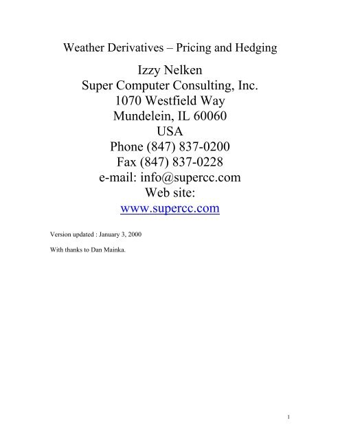
<strong>Weather</strong> <strong>Derivatives</strong> <strong>–</strong> <strong>Pricing</strong> <strong>and</strong> <strong>Hedging</strong>Izzy Nelken<strong>Super</strong> <strong>Computer</strong> Consulting, Inc.1070 Westfield WayMundelein, IL 60060USAPhone (847) 837-0200Fax (847) 837-0228e-mail: info@supercc.comWeb site:www.supercc.comVersion updated : January 3, 2000With thanks to Dan Mainka.1
On the day following the expiration of the option, that is April 1, 2000 we can computethe payoutPayout = min(Dollars per unit * max(Total-Strike, 0), Maximal payout)In our example,Payout = min($10,000 * max(Total-5000, 0), $2,000,000)The party who buys this option will be paid if the winter in Chicago will be severe. Inthat case, the winter will be cold, a lot of HDD’s will be generated <strong>and</strong> Total would belarge. Thus call options pay out in extreme weather conditions <strong>and</strong> put options pay outwhen the weather is mild.Actually, the payout of this option shows a greater similarity to a traditional call spreadrather than to a call option. Note that our option can not be in the money by more than200 HDD’s.In addition to put <strong>and</strong> call options, there have been some trading in digital options, barrierstructures <strong>and</strong> even compound options.MotivationThere are many institutions whose profit <strong>and</strong> loss are severely impacted by the weather.For example, farmers whose crop will be ruined if the weather is too warm, may desirethese options as a hedge. Other potential clients are clothing manufacturers <strong>and</strong> retailerswhose livelihood depends on cold winters. Tour operators, hotels <strong>and</strong> many types ofseasonal businesses could also benefit. The US Department of Commerce estimates thatweather impacts businesses representing $1 trillion of the $9 trillion US gross domesticproduct.In addition, small institutions on the buy side may be wary of purchasing options ontraded commodities. An often-expressed fear is that the big banks on the sell side willtrade in the spot market in such a way as to cause some barrier options to knock out.However, even the largest sell side dealer can not influence the weather.<strong>Pricing</strong>Black ScholesThe Black Scholes pricing methodology is based on continuous hedging. This methodworks well when pricing options on currencies, stocks, commodities or other fungibleassets which can be traded in the spot market. The difficulty with the weather derivativesis that the underlying is not traded. “You can not buy a sunny day” goes the old saying.3
Burn AnalysisAnother approach is practiced in the insurance industry. One may ask the question: “whatwould we have paid out had we sold a similar put option every year in the past fiftyyears?”The method proceeds as follows:1) Collect the historical weather data.2) Convert to degree days (HDD or CDD).3) Make some corrections.4) For every year in the past, determine what the option would have paid out.5) Find the average of these pay out amounts.6) Discount back to the settlement date.This method is known as “burn analysis”. Much of the difficult work is in stages 1 <strong>and</strong> 3.Collecting the historical data may be somewhat difficult. While there are web sites withdownloadable historical weather information for the USA, obtaining historical weatherdata for the United Kingdom is quite costly. Even when the data is available, there aremissing data, gaps <strong>and</strong> errors. The historical data must be “scrubbed” before it is used forpricing.The correction step is also challenging. Here are some issues:1) The period in question is a leap year. Thus there are more days in the periodNovember 1, 1999 <strong>–</strong> March 31, 2000 than there are in the corresponding period(November 1, 1998 <strong>–</strong> March 31, 1999) the year before. This is due to theexistence of February 29, 2000, a date that did not exist in 1999.2) The weather station may have had to be moved due to construction. Alternatively,it may have been in the sun <strong>and</strong> now it is in the shade etc.3) How many years of historical data should one consider? Should you look at tenyears? Twenty? Or even more?4) Many cities exhibit the “urban isl<strong>and</strong> effect”. Due to heavy industrial activity,construction <strong>and</strong> pollution, the weather gradually becomes warmer in that area. Infact, in some urban centers, it is possible to detect warming trends in the weather.These trends must be accounted for when pricing the option.5) There are extreme weather patterns that occur in some years. Most notable are theEl Nino <strong>and</strong> La Nina. Basically, the El Nino is the warming of the water in theeastern <strong>and</strong> central equatorial Pacific Ocean. La Nina is the opposite effect whenthe same areas of the Pacific are cooler than average. The pricing of an option in ayear that is forecast to be El Nino is different than in a year that is not.4
In any case, it is possible to resolve these problems in a reasonable manner. A weathertrend may be corrected for by observing the average HDD’s for the past ten years <strong>and</strong>comparing it with the corresponding trailing ten year average of the HDD’s for each ofthe years in the past. For example, assume that• For the year 1988, in the period November 1, 1988 to March 1, 1989 theHDD count was 5050.• The average of the HDD counts for the ten years 1989 to 1998 was 5000.• The average of the HDD counts for the ten years preceding <strong>and</strong> including1988, which are 1979 to 1988, was 5020.When we compare the average HDD counts in that city, we find that the HDD’s havedropped from 5020 to 5000. This is consistent with a warming of the weather. In thiscase, it may be reasonable to shift the data relating to 1988. A linear shift would beShifted HDD = Observed HDD + last average <strong>–</strong> previous average = 5050 + (5000-5020)= 5030It is also possible to find reasonable corrections for the other effects.Most market participants use some sort of burn analysis in computing the fair value of theoption. These “degree day based models” are simple to construct. All that is required is agood source of historical data.A FlawThere is a serious flaw in the degree day based models such as the burn analysis. Thisflaw manifests itself most profoundly in periods when temperatures hover around 65degrees. In most areas of the US, these are typically the fall <strong>and</strong> autumn seasons, socalled the “shoulder months”.To observe this flaw, consider a simple contrived hypothetical example. Consider anoption whose period is three days: February 3, 4 <strong>and</strong> 5, 2000.We observe the historical weather in City A:Feb 3 Feb 4 Feb 51996 64 64 641997 66 66 661998 64 64 641999 67 67 67We also observe the historical weather in City B:Feb 3 Feb 4 Feb 51996 64 64 641997 96 96 965
1998 64 64 641999 97 97 97Obviously these two cities exhibit totally different weather patterns. We would not wantto sell a weather derivative on City A for the same price as a weather derivative on CityB.Note, however, that any degree day bases model (including the burn analysis describedabove) would not be able to distinguish between these two cities.The HDD’s generated are exactly the same for both cities:1996 31997 01998 31999 0Any degree day based model can not differentiate between City A <strong>and</strong> City B. Theproblem is due to the cutoff at 65 degrees.Another FlawWhat is the level of a zero cost swap? Under burn rate analysis, the answer to thisquestion depends on the maximal payout assumption. This seems highly non-intuitive, aswe would expect that the strike of a zero cost collar would be the same no regardless ofthe maximal payout amount.For example, consider a swap in which we are long HDD in Chicago. The period isNovember 1, 1999 to March 31, 2000. Assume that there is a $10,000 payment per HDD<strong>and</strong> that the maximal payout is $10,000,000.Taking the last ten years of data (1989-1998), without trending or adjusting for leapyears, we note that the average HDD level is 5018.75. A swap with a level of 5018.75would indeed be a zero-cost swap.On the other h<strong>and</strong>, assume that the maximal amount that can be paid out (either way)under the swap is only $1,700,000. In this case, the burn analysis gives a totally differentresult. A swap with a level of 5018.75 would actually show an average payout of about($202,000). That’s right, the average payout of this swap would be approximatelynegative $202,000!If we restrict the maximal payout, then in some of the ten years of history we would getthe maximal payout of $1,700,000 <strong>and</strong> in some we would pay it. The average of thesepayouts will not, in general, be zero. In some cases (as in our example) it would be verydifferent from zero. To make the average payout zero, we would have to change theswap’s level to 4945.6
In summary, if the maximal payout of the swap is $10,000,000 then the level of a zerocost swap is 5018.75. On the other h<strong>and</strong>, if the maximal payout is $1,700,000 then thelevel of the zero cost swap becomes 4945.The problem does not disappear even if we used more data. Using thirty years ofhistorical data gives very similar results.This very un-intuitive result stems from the fact that we are using a burn rate analysis <strong>and</strong>that the options’ payout is bounded.Temperature Based ModelsMore sophisticated weather derivative models are based on modeling the weatherdirectly. These models do not incur the flaws mentioned above.Such models have the following steps:1) Collect the historical weather data.2) Make some corrections.3) Create a statistical model of the weather.4) Simulate possible weather patterns in the future.5) For each weather pattern, calculate the payout of the option.7) Find the average of these pay out amounts.8) Discount back to the settlement date.The fundamental difference between the two approaches is that we are building a modelfor the weather, not the degree days.The simulation done in step 4 could be performed using a Monte Carlo algorithm. Suchalgorithms generate r<strong>and</strong>om numbers. These r<strong>and</strong>om numbers are then used to simulatethe behavior of the phenomena we are trying to model.It is possible to price foreign exchange options using the Monte Carlo algorithm. Mostmarket participants agree that foreign exchange fluctuates according to a r<strong>and</strong>om walkdescribed by a geometric Brownian motion:The stochastic process is described by the differential equation:dP = (r-q)P dt + σ P dzHereP is the price of the security (or the foreign exchange rate)dP is the instantaneous change to the price Pdt is an infinitesimally small unit of timer is the domestic interest rate of the payout currency7
q is the foreign interest rateσ is the annualized volatility of the exchange ratedz is a Weiner process based on a normal distribution with a mean of zero <strong>and</strong> a st<strong>and</strong>arddeviation of 1:It is possible, <strong>and</strong> not too difficult, to show that an algorithm which involves runningmany simulations of this Monte Carlo algorithm, taking the final exchange rate on theexpiration of the option, computing the payout of the option for each of the simulations,averaging these payouts <strong>and</strong> discounting the average back to the settlement date will giveprecisely the same results as the Black Scholes formula.Can we use the same model for temperature?Unfortunately not. It is possible for exchange rates or stock prices to fluctuate sharplyover time. For example, many stocks have doubled their value within one year. However,it seems unlikely that the temperature next year will be double of what it was this year.We therefore choose a different model for the weather. To model weather, we decided touse mean reverting models.Mean Reverting ModelsMean reverting models have been used extensively to model interest rates. In the US,where interest rates are approximately 5%, it is unlikely that rates will be 50%.There are many different models of interest rates. For an excellent review of the differentmodels, see the chapter by Kerry Back in my book “Option Embedded Bonds”, IrwinProfessional Publishing (ISBN 0-7863-0818-4).To illustrate a mean reverting model, consider the “simple Gaussian model”. Thedifferential equation describing the model is given by:dr = a*(b-r) dt + σ dzHerer is the continuously compounded instantaneous interest ratedr is the instantaneous change in rdt is an infinitesimally small unit of timeb is the mean interest ratea is the speed of mean reversion.σ is the volatilitydz is a Weiner process based on a normal distribution with a mean of zero <strong>and</strong> a st<strong>and</strong>arddeviation of 1:8
This is an example of a simple “mean reverting” model. Intuitively, r, the instantaneousinterest rate changes by an amount equal to dr. In this model, it is assumed that interestrates will converge to some “long term mean” b. If r is greater than b then thecontribution (b-r) s negative. This will tend to pull interest rates to a lower level.Similarly, if r is less than b, then (b-r) is positive which will tend to pull interest ratehigher.The term (b-r) is the “pull to the mean”. It is multiplied by a, the “speed of meanreversion” <strong>and</strong> this is added to the term dr.In addition, there is a r<strong>and</strong>om component to the short term interest rate. The r<strong>and</strong>omcomponent is represented by the term σ dz.dz is a Weiner process that is based on a normally distributed r<strong>and</strong>om variable which hasa mean of zero <strong>and</strong> a st<strong>and</strong>ard deviation of one. Thus the r<strong>and</strong>om component may bepositive or negative.Mean reverting models, similar to the “simple Gaussian”, are used to price interest rateoptions, such as caps, floors <strong>and</strong> swaptions. There is an active <strong>and</strong> liquid market forinterest rate derivatives based on the Libor (London Interbank Offered Rate). Indeed, themost liquid at the money caps will be offered by various dealers at prices that are within0.1 basis points of each other.The main difficulty lies in determining the various parameters: a,b <strong>and</strong> σ. Obviously,once the parameters are known, it is possible to compute the prices of various derivativeinstruments. Calibration is the reverse process in which the market prices of the liquidderivative instruments are used to determine the parameters of the model. We are tryingto determine the set of model parameters that would result in prices that are as close aspossible to the market prices on a large variety of instruments.Intuitively, calibration answers the question:“What is the set of model parameters that would result in the model matching theobserved market prices or as coming as close to them as possible”Model calibration is quite computationally intensive <strong>and</strong> typically requires highdimensional non-linear optimization. Of course, it relies on the availability of marketprices for the liquid instruments.Some questionsIt is natural to assume a mean reverting model for the weather. Just like interest rates, it isunlikely that the weather next year will be ten times higher than the weather this year.Before embarking on designing a mean reverting model for the weather, though, we needto ascertain if such a model describes the weather reasonably well.9
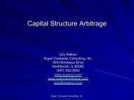
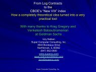
One question to ask is: “Is the weather distributed normally around its mean?”In Figure 1 we plot the Cumulative Distribution Function (CDF) of the weather in aparticular weather station (Chicago). We compare the CDF to the one generated by anormal distribution. In most cases, the observed CDF of the weather closely matches theCDF of a normal distribution. There is several statistical test to quantify the “goodness ofthe fit”. One such test is the Kolmogrov-Smirnov (KS) test. The KS test measures themaximal distance between the hypothetical CDF <strong>and</strong> the observed one. This is termed the“ks score”. Based on the “ks score”, the probability that the distribution is not normal isdisplayed. Obviously, high ks scores would imply a high probability that the distributionis not normal.For Chicago, in 42 days (out of 366), one is able to reject the hypothesis that the weatheris distributed normally. In the remaining 324 days, we can not reject the hypothesis thatthe weather is distributed normally. Since the normal distribution assumption holds wellfor about 88% of the cases, we have decided to use it.These results are quite typical. In extensive tests over many different weather stations,we’ve noticed that we can reject the normal distribution in about 10-20% of the days.Another question that we may ask concerns the degree of the model.When you are modeling tomorrow’s temperature, you should obviously use thetemperature from today. However, should you also use the temperature from yesterday aswell as the day before yesterday? What about 50 days ago?We can write this as an equation:W(T+1) = F(W(T), W(T-1), … , W(T-n))Where, W(T+1) is the weather tomorrow, W(T) is the weather today, W(T-n) is theweather n days ago <strong>and</strong> F is some unspecified function.How many days from the past should we use. What should n be? Models in which n iszero, are called memory-less. In other words, they exhibit a Markov property.This concerns the auto-correlation between the temperatures. In Figure 2, we plot theauto-correlation for a particular weather station (Chicago). Naturally, the weather oneach day has a perfect correlation with itself. Thus for a lag of zero, the correlation is 1.If we allow a one day lag, the correlation is quite high (about 0.7). Note that thecorrelation decreases as we increase the lag.If the correlation between W(T+1) <strong>and</strong> W(T-n) is exactly zero, then no new informationadded by using that day. It is almost impossible to see a correlation of exactly zerobetween any two series. However, if the correlation is small enough <strong>and</strong> is close to zero,then very little information is added by using that day.10
Figure 2 shows that there is some correlation even when n is 25. In general, the higher thenumber n, the more precise our model. On the other h<strong>and</strong>, the higher the number n, themore parameters that will have to be estimated. This will cause the calibration process tobe more complicated. That is, we would have to determine exactly how W(T-n) impactson W(T+1). As n increases <strong>and</strong> the correlation decreases, the effect becomes subtle <strong>and</strong>more difficult to determine.We have only a limited amount of historical weather information <strong>and</strong> the observedweather in the past is subject to r<strong>and</strong>om fluctuations. This causes “parameter estimationerrors”. The relative importance of these errors grows with n.When designing a weather model, what n should one choose? Because of the difficultiescaused by the parameter estimation errors, we have decided to use n=0. Thus our modelsassume that the weather is a Markov process. Obviously, this is only an approximation.However, given the realities of the market place <strong>and</strong> the available data, we felt that thiswas the best choice.A Model for <strong>Weather</strong>Our model is similar to the models used in interest rate derivatives. However, there are afew caveats:1) The weather changes with the season. Hence we allow the mean of the weather tovary. The parameter representing the mean, b, is replaced with b(i), whichrepresents the mean for day number i.2) Similarly, the volatility may depend on the day in question. In many cities (e.g.Chicago) the weather is more volatile in the winter than in the summer. Thevolatility parameter σ is changed to σ (i), the volatility for a particular day.3) By the same token, we allow the mean reversion rate to vary. The parameter a,which represents the mean reversion rate is allowed to change over time. Themean reversion rate for day i is represented by a(i).4) There is a natural seasonal effect in weather. Assume that it is now spring <strong>and</strong> thatthe temperature today is exactly equal to its long term mean. We may well expectthat the temperature tomorrow will be slightly warmer than it is today. In otherwords, there is a natural “drift” to the weather.The most important difference between interest rate derivative models <strong>and</strong> models forweather derivatives is the calibration process.• Interest rate derivative models are calibrated to the market prices of liquidinstruments. This calibration process was described above.• <strong>Weather</strong> derivative models are calibrated to past data.As yet, an active <strong>and</strong> liquid market does not yet exist for weather derivatives. On theother h<strong>and</strong>, we have a wealth of historical weather data.11
The calibration process asks:“What is the set of model parameters that would have the highest probability ofgenerating the past weather patterns?”This is essentially a “maximum likelihood” question. Assume that the observed data isthe result of a stochastic process. We are determining the parameters for which theprobability of having generated the observed data is maximal.For example, consider that you flip a coin 1000 times. It comes out 900 heads <strong>and</strong> 100tails. It could be that this is a fair coin <strong>and</strong> that this is an unlikely sequence of coin flips.On the other h<strong>and</strong>, it could be that the coin is not even <strong>and</strong> intrinsically has a much higherchance of showing heads than tails. The maximum likelihood technique would tend tochoose the second explanation.To summarize, the weather derivative model works as follows:1) It calibrates the model to the observed past data using a maximum likelihoodtechnique.2) Once the model parameters are determined, weather sequences are generatedusing a Monte Carlo process.3) The r<strong>and</strong>om sequences drive a mean reverting model, similar to models used toprice interest rate derivatives.4) Many sequences are generated. Each sequence represents a possible futureweather pattern. For each weather sequence, the payout of the option isdetermined.5) The average payout of the option under the various scenarios is deemed to bethe expected payout of the option.6) Taking the present value of the expected payout gives us a fair value price.<strong>Hedging</strong> of <strong>Weather</strong> <strong>Derivatives</strong>Option traders, including equity <strong>and</strong> foreign exchange option traders, utilize a techniqueknown as “delta hedging”. Delta hedging entails computing the sensitivity of an option’sprice to a change in the underlying <strong>and</strong> buying or selling an appropriate amount ofunderlying instruments. For example, suppose a dealer sold an at the money call optionwith a delta of 0.50. This means that for every $1 rise in the price of the underlying stock,the option’s price will rise by $0.50. A dealer who sells such a call option immediatelybuys 0.50 units of stock. If the stock rises by $1, the dealer will lose $0.50 on his optionposition but will gain $0.50 because he is long shares.The difficulty in hedging weather derivatives lies in the fact that one can not purchase orsell the underlying instrument. As the saying goes “You can’t buy a sunny day”.<strong>Weather</strong> derivative dealers hedge themselves using a variety of techniques, including:12
1) Limiting the potential loss on an option. All weather derivatives have a cap on themaximal payout. This is quite different than traditional options (e.g. on equities orforeign exchange) that typically do not have caps on the maximal payoutamounts.2) Running a well diversified, balanced book. Dealers try to buy <strong>and</strong> sell manyweather derivatives that are based on both HDD <strong>and</strong> CDD in many differentcities. Even if the weather deviates from normal by a lot in one part of the country<strong>and</strong> causes a loss to the dealer, it is highly unlikely that the dealer will lose on allopen option positions. Note that dealers have to assume some correlation (or lackof correlation) between the various weather stations. Such assumptions can betested on past data. In this fashion, the weather derivative dealer is essentiallyworking like an insurance company. An insurance company sells many carinsurance policies <strong>and</strong> buys some re-insurance products. Unfortunately, a wellbalanced book is difficult to create a small weather derivative business.3) Selling options that are long term. A typical option sums up all the degree daysbetween November 1 <strong>and</strong> March 31 of the following year. Even if the weather isunseasonably warm on a particular day, it is unlikely to stay extremely warmduring the entire five months. A dealer would be hard pressed to sell a weatherderivative that is settled based on the weather on a single day. The summationeffect reduces the variability of the pay out.One hedging technique that is available is to hedge with zero cost swaps.Assume that a dealer sells a 5000 HDD call option on Chicago. The option runs fromNovember 1 to March 31. It pays $10,000 per HDD with a maximal payout of$2,000,000. Here are some modeling results:Sold P&L on Call Buy Sell price of P&L of swapATM DD 5000 Call 5016 call 5016 Put swap4,966 $709,649 $ 113,104 $668,830 $869,192 $ (200,362) $ (200,216)5,016 $822,753 $782,386 $782,532 $ (146)5,066 $910,081 $ (87,329) $889,733 $725,206 $ 164,527 $ 164,673Assume that the zero cost swap strike price is 5,016.The price of the 5,000 call option which was sold by the dealer is $822,753.Assume that several days have past <strong>and</strong> that the forecasters change their prediction.Based on new information they predict that the winter will be slightly milder thanusual. That would mean that the strike of the zero cost swap would move downwards.Assume that it would change to 4,966.If the zero cost swap strike was to move by 50 HDD to 4,966 the price of the 5,000call would decline to $709,649 <strong>and</strong> the dealer would show a profit of $113,104. Onthe other h<strong>and</strong> if the zero cost swap strike was to move by 50 HDD to 5,066 thedealer would show a loss of $87,329.13
Let’s consider the 5,016 swap. The swap consists of a long position in a 5,016 calloption <strong>and</strong> a short position in a 5,016 put option. Both options have a payout of$10,000 per HDD with a maximal payout of $2,000,000When the at the money swap strike is 5,016, the price of the call almost exactlyoffsets the price of the put <strong>and</strong> the cost of the swap is zero (a zero cost swap).If the zero cost swap strike was to move to 4,966 the price of the 5,016 swap woulddecrease by $200,216. On the other h<strong>and</strong>, if the zero cost strike price would increaseto 5,066 the price of the 5,016 swap would increase by $164,673.As the dealer does not know what the future will bring, he should hedge himself byentering into a fractional amount of a swap. The amount of swap entered in thisexample would be:($113,104- (-$87,329) ) / ($164,673 <strong>–</strong> (-200,216)) = 0.549Note that the “delta” of the call option is 0.549. We expect the delta of a slightly inthe money call option to be slightly greater than 0.5. Also note that the profit on oneside $113,104 does not exactly match the loss on the other side $87,329. This is dueto the gamma effect. The delta of the option changes as the strike of the at the moneyswap increases or decreases.Therefore, our dealer could enter into 0.549 units of swap for every call option sold.In reality, the dealer would probably adjust the payout amounts per HDD <strong>and</strong> themaximal payout amount.Assume that the 5,016 options entered into as the swap position were to be changes sothat the payout is $5490 per degree day <strong>and</strong> the maximal payout is $1,098,000.We now repeat the calculations as above:Buy Sell price of swap P&L of swapATM DD 5016 call 5016 Put4966 $ 376,427 $ 479,616 $ (103,189) $ (103,376)5016 $ 431,435 $ 431,248 $ 1875066 $ 487,091 $ 399,120 $ 87,971 $ 87,784We note that the profit <strong>and</strong> loss on the swap almost matches the profit <strong>and</strong> loss on theoption exactly.In a traditional delta hedging approach, the dealer would constantly adjust his deltahedge ratio <strong>and</strong> increase or decrease his exposure to the swap. This may be very14
costly to do in the weather derivatives market as the instruments are not liquid.Therefore, if dealers use delta hedging at all, they would hedge only at the beginningof the trade <strong>and</strong> will typically not re-balance at all.SummaryTo summarize, the weather derivative product is rapidly developing. While its originsas an insurance policy explain the usage of techniques such as “burn analysis”, theyare quite inadequate to price these options. We have developed techniques, models<strong>and</strong> tools that are based on interest rate pricing analytics. It is only a matter of timeuntil such models are adapted by the industry.15
Appendix: Figures0.0 0.2 0.4 0.6 0.8 1.00.0 0.2 0.4 0.6 0.8 1.0Empirical <strong>and</strong> Hypothesized normal CDFsChicago - O'Hare (WBAN: 94846)-10 0 10 20 30 40solid line is the empirical d.f.Day: 01/20Empirical <strong>and</strong> Hypothesized normal CDFsChicago - O'Hare (WBAN: 94846)20 30 40 50 60solid line is the empirical d.f.Day: 03/260.0 0.2 0.4 0.6 0.8 1.00.0 0.2 0.4 0.6 0.8 1.0Empirical <strong>and</strong> Hypothesized normal CDFsChicago - O'Hare (WBAN: 94846)0 10 20 30 40solid line is the empirical d.f.Day: 02/06Empirical <strong>and</strong> Hypothesized normal CDFsChicago - O'Hare (WBAN: 94846)40 50 60 70solid line is the empirical d.f.Day: 04/11Figure 1: Several days <strong>and</strong> their Cumulative Distribution Functions (CDF) as comparedwith the normal distribution. Note the goodness of the fit.16
1Autocorrelation of Station (WBAN): 94846 (Untrended/Unsmoothed)Correlation Coefficient0.90.80.70.60.50.40.30.20.10-30 -20 -10 0 10 20 30Lag/LeadFigure 2: Autocorrelation of the temperatures.17