Land Use Change and its Impact on Selected Biophysical and ...
Land Use Change and its Impact on Selected Biophysical and ...
Land Use Change and its Impact on Selected Biophysical and ...

You also want an ePaper? Increase the reach of your titles
YUMPU automatically turns print PDFs into web optimized ePapers that Google loves.
KFRI Research Report No.298 ISSN 09708103<str<strong>on</strong>g>L<str<strong>on</strong>g>and</str<strong>on</strong>g></str<strong>on</strong>g> <str<strong>on</strong>g>Use</str<strong>on</strong>g> <str<strong>on</strong>g>Change</str<strong>on</strong>g> <str<strong>on</strong>g>and</str<strong>on</strong>g> <str<strong>on</strong>g>its</str<strong>on</strong>g> <str<strong>on</strong>g>Impact</str<strong>on</strong>g> <strong>on</strong> <strong>Selected</strong> <strong>Biophysical</strong><str<strong>on</strong>g>and</str<strong>on</strong>g> Socioec<strong>on</strong>omic Aspects of Karuvannur River Basinin Thrissur District of KeralaP.K. MuraleedharanJose KallarackalA.R.R. Men<strong>on</strong>M. BalagopalanN. SasidharanP. RugminiKerala Forest Research InstituteAn Instituti<strong>on</strong> of Kerala State Council for Science, Technology <str<strong>on</strong>g>and</str<strong>on</strong>g> Envir<strong>on</strong>mentPeechi 680 653, Thrissur, KeralaK F R INovember 2007
ABSTRACT OF THE PROJECT PROPOSAL1. Project No : KFRI/421/042. Title : <str<strong>on</strong>g>L<str<strong>on</strong>g>and</str<strong>on</strong>g></str<strong>on</strong>g> use change <str<strong>on</strong>g>and</str<strong>on</strong>g> <str<strong>on</strong>g>its</str<strong>on</strong>g> impact <strong>on</strong> selectedbiophysical <str<strong>on</strong>g>and</str<strong>on</strong>g> socioec<strong>on</strong>omic aspects of KaruvannurRiver Basin in Thrissur district of Kerala3. Objectives : Study the nature <str<strong>on</strong>g>and</str<strong>on</strong>g> extent of l<str<strong>on</strong>g>and</str<strong>on</strong>g>use <str<strong>on</strong>g>and</str<strong>on</strong>g>cropping pattern changes <str<strong>on</strong>g>and</str<strong>on</strong>g> important socioec<strong>on</strong>omic drivers affecting it.4. Date of commencement : February 20045. Date of completi<strong>on</strong> : April 2007: Examine the effects of l<str<strong>on</strong>g>and</str<strong>on</strong>g>use <strong>on</strong> hydrology runoff,stream flow, ground water table, temperature<str<strong>on</strong>g>and</str<strong>on</strong>g> humidity in the watershed.: Analyze the effects of l<str<strong>on</strong>g>and</str<strong>on</strong>g>use/cropping pattern changes<strong>on</strong> vegetati<strong>on</strong>, sedimentati<strong>on</strong>, agricultural producti<strong>on</strong><str<strong>on</strong>g>and</str<strong>on</strong>g> socioec<strong>on</strong>omic c<strong>on</strong>diti<strong>on</strong>s of the people.: Assess ec<strong>on</strong>omic value of water resource, surfacewater use pattern, pricing <str<strong>on</strong>g>and</str<strong>on</strong>g> use c<strong>on</strong>flict over waterresources am<strong>on</strong>g different secti<strong>on</strong>s in the society.: Examine the linkages between ecological <str<strong>on</strong>g>and</str<strong>on</strong>g> socioec<strong>on</strong>omicsystems of the upl<str<strong>on</strong>g>and</str<strong>on</strong>g> <str<strong>on</strong>g>and</str<strong>on</strong>g> downstream areasof the watershed in determining overall development.6. Funding Agency : Ministry of Envir<strong>on</strong>ment <str<strong>on</strong>g>and</str<strong>on</strong>g> Forests7. Investigators : P.K. MuraleedharanJose KallarackalA.R.R. Men<strong>on</strong>M. BalagopalanN. SasidharanP. Rugmini8. Research Fellows : John P. Inchakalody, P. Muhammed Rasheed <str<strong>on</strong>g>and</str<strong>on</strong>g>U.V. Deepa9. Study area : Karuvannur River Basin
CONTENTSACKNOWLEDGEMENTSABSTRACTi1. INTRODUCTION 11.1. The study area 21.2. Ecological <str<strong>on</strong>g>and</str<strong>on</strong>g> ec<strong>on</strong>omic problems in the study area 51.3. Objectives 72. METHODOLOGY 92.1. Selecti<strong>on</strong> of micro watersheds 92.2. <str<strong>on</strong>g>L<str<strong>on</strong>g>and</str<strong>on</strong>g></str<strong>on</strong>g> use dynamics 92.3. Vegetati<strong>on</strong> classificati<strong>on</strong> scheme 102.4. Digital classificati<strong>on</strong> of satellite data 112.5. Vegetati<strong>on</strong> characterizati<strong>on</strong> using satellite data 112.6. Accuracy evaluati<strong>on</strong> 122.7. Hydro meteorological observati<strong>on</strong>s 162.8. Water table fluctuati<strong>on</strong> studies 172.9. Socioec<strong>on</strong>omic aspects 182.10. Ec<strong>on</strong>omic valuati<strong>on</strong> of water resources 193. LAND USE AND CROPPING PATTERN CHANGES 273.1. <str<strong>on</strong>g>L<str<strong>on</strong>g>and</str<strong>on</strong>g></str<strong>on</strong>g> use change 273.2. Cropping pattern 333.3. <str<strong>on</strong>g>L<str<strong>on</strong>g>and</str<strong>on</strong>g></str<strong>on</strong>g> use <str<strong>on</strong>g>and</str<strong>on</strong>g> cropping pattern changes: Biophysical <str<strong>on</strong>g>and</str<strong>on</strong>g> socioec<strong>on</strong>omic drivers 354. HYDROLOGICAL STUDIES 414.1. Historical data <strong>on</strong> annual rainfall distributi<strong>on</strong> 414.2. Average seas<strong>on</strong>al stream discharge at the study area 524.3. Ground water table 544.4. Water level in Peechi Reservoir 604.5. Temperature <str<strong>on</strong>g>and</str<strong>on</strong>g> relative humidity 624.6. Seas<strong>on</strong>al distributi<strong>on</strong> of temperature 634.7. Relative humidity 644.8. Discussi<strong>on</strong> 65
5. EFFECTS OF LAND USE/CROPPING PATTERN CHANGES ON VEGETATION,SEDIMENTATION AND SOCIOECONOMIC CONDITIONS OF THE PEOPLE 715.1. Plant diversity in the Olakara watershed area 715.2. Vegetati<strong>on</strong> analysis 725.3. Sedimentati<strong>on</strong> 755.4 Increase of producti<strong>on</strong> <str<strong>on</strong>g>and</str<strong>on</strong>g> productivity in agricultural sector 785.5. Socioec<strong>on</strong>omics 796. VALUATION OF WATER RESOURCES AND USE CONFLICTS 836.1. Direct extractive benef<str<strong>on</strong>g>its</str<strong>on</strong>g> 836.2. Direct n<strong>on</strong>extractive benef<str<strong>on</strong>g>its</str<strong>on</strong>g> 846.3. Dem<str<strong>on</strong>g>and</str<strong>on</strong>g> functi<strong>on</strong> of tourists of Peechi Dam 846.4. Total recreati<strong>on</strong>al value 866.5. Indirect use value 866.6 Total estimated ec<strong>on</strong>omic value 866.7. Pricing of water: some issues 876.8. Willingness to pay 896.9. Water use c<strong>on</strong>flict 916.10. Sources of water in the study area 916.11. Irrigati<strong>on</strong> vs. Drinking water 926.12. C<strong>on</strong>flict am<strong>on</strong>g farmers 946.13. Local level c<strong>on</strong>flicts 957. LINKAGES BETWEEN UPLAND AND DOWN STREAM AREAS 97Upl<str<strong>on</strong>g>and</str<strong>on</strong>g> 97<str<strong>on</strong>g>Change</str<strong>on</strong>g>s in downstream areas 98Envir<strong>on</strong>mental problems 1018. CONCLUSIONS AND RECOMMENDATIONS 103REFERENCES 107APPENDIX 113
ACKNOWLEDGEMENTSThe project was sp<strong>on</strong>sored by Ministry of Envir<strong>on</strong>ment <str<strong>on</strong>g>and</str<strong>on</strong>g> Forests, NewDelhi. We wish to place <strong>on</strong> record our sincere thanks to Dr. R.Gnanaharan, Director <str<strong>on</strong>g>and</str<strong>on</strong>g> Dr. J.K. Sharma, former Director, KeralaForest Research Institute for kind support <str<strong>on</strong>g>and</str<strong>on</strong>g> encouragement. We arealso placing <strong>on</strong> record our sincere gratitude to Shri. Ashok Bhatia,Additi<strong>on</strong>al Director, Ministry of Envir<strong>on</strong>ment <str<strong>on</strong>g>and</str<strong>on</strong>g> Forests, who washelpful during the project period. We express our sincere thanks to Dr.K.C. Chacko, Dr. S.Sankar, <str<strong>on</strong>g>and</str<strong>on</strong>g> Dr. M.P.Sujatha of the Institute foreditorial scrutiny. We are extremely thankful to Mr. John P. Inchakalody,Mr. P. Muhammed Rasheed <str<strong>on</strong>g>and</str<strong>on</strong>g> Ms. U.V. Deepa, Research Fellows whocollected data for the study. We are grateful to Dr.Jagdish Krishnaswamy(ATREE) <str<strong>on</strong>g>and</str<strong>on</strong>g> Dr. S. Sankar for useful suggesti<strong>on</strong>s during the initial stagesof the project. The help rendered by Dr. K. Sreelakshmi <str<strong>on</strong>g>and</str<strong>on</strong>g> Dr. V. Anithadeserves special thanks. Thanks are also due to our colleagues in theInstitute who offered comments at the time of presentati<strong>on</strong> of the resultsof the study.
ABSTRACTDegradati<strong>on</strong> of watersheds is <strong>on</strong>e of the major problems in Kerala, whichhas brought about ineffaceable <str<strong>on</strong>g>and</str<strong>on</strong>g> irreversible l<str<strong>on</strong>g>and</str<strong>on</strong>g>use <str<strong>on</strong>g>and</str<strong>on</strong>g> ecologicalchanges, leading to impairment of <str<strong>on</strong>g>its</str<strong>on</strong>g> hydrological functi<strong>on</strong>s. Unscientificl<str<strong>on</strong>g>and</str<strong>on</strong>g>use <str<strong>on</strong>g>and</str<strong>on</strong>g> cropping pattern changes in a watershed often causeproblems in water c<strong>on</strong>servati<strong>on</strong> both in upl<str<strong>on</strong>g>and</str<strong>on</strong>g> <str<strong>on</strong>g>and</str<strong>on</strong>g> downstream areas.This accelerates the runoff rate <str<strong>on</strong>g>and</str<strong>on</strong>g> soil erosi<strong>on</strong> <str<strong>on</strong>g>and</str<strong>on</strong>g> alters stream flowquality <str<strong>on</strong>g>and</str<strong>on</strong>g> quantity, which in turn affect <strong>on</strong>site producti<strong>on</strong> <str<strong>on</strong>g>and</str<strong>on</strong>g>/or offsiteproducti<strong>on</strong> or c<strong>on</strong>sumpti<strong>on</strong>. In a watershed both upl<str<strong>on</strong>g>and</str<strong>on</strong>g> <str<strong>on</strong>g>and</str<strong>on</strong>g> downstream areas are closely interlinked. However, the nature <str<strong>on</strong>g>and</str<strong>on</strong>g> extent oftheir interlinkage, especially in a forested watershed has not been studiedin depth in Kerala. This study is a modest attempt to fill this gap.Manali watershed of Karuvannur River Basin, where a major part of theforest area of the basin is located, was selected for detailed study. Thebroad objective was to examine l<str<strong>on</strong>g>and</str<strong>on</strong>g>use change <str<strong>on</strong>g>and</str<strong>on</strong>g> <str<strong>on</strong>g>its</str<strong>on</strong>g> effects <strong>on</strong> ecohydrology<str<strong>on</strong>g>and</str<strong>on</strong>g> socioec<strong>on</strong>omic c<strong>on</strong>diti<strong>on</strong>s of the people in the study area.Specific attempts were made to study the nature, extent <str<strong>on</strong>g>and</str<strong>on</strong>g> socioec<strong>on</strong>omicfactors affecting l<str<strong>on</strong>g>and</str<strong>on</strong>g>use changes <str<strong>on</strong>g>and</str<strong>on</strong>g> forest degradati<strong>on</strong> <str<strong>on</strong>g>and</str<strong>on</strong>g> <str<strong>on</strong>g>its</str<strong>on</strong>g>effects <strong>on</strong> sediment producti<strong>on</strong> <str<strong>on</strong>g>and</str<strong>on</strong>g> water discharge rates <str<strong>on</strong>g>and</str<strong>on</strong>g> <strong>on</strong>site <str<strong>on</strong>g>and</str<strong>on</strong>g>offsite agricultural producti<strong>on</strong>. Assessment of surface runoff <str<strong>on</strong>g>and</str<strong>on</strong>g> streamflow from watersheds, ec<strong>on</strong>omic value of water resource, surface wateruse pattern, pricing <str<strong>on</strong>g>and</str<strong>on</strong>g> use c<strong>on</strong>flict over water resources am<strong>on</strong>g differentsecti<strong>on</strong>s in the society was also made. Further it examined linkagesbetween ecological <str<strong>on</strong>g>and</str<strong>on</strong>g> socioec<strong>on</strong>omic systems of the upl<str<strong>on</strong>g>and</str<strong>on</strong>g> <str<strong>on</strong>g>and</str<strong>on</strong>g>downstream areas of the watershed in determining overall development.A nested catchment approach was used to select upstream <str<strong>on</strong>g>and</str<strong>on</strong>g> downstream areas of the watershed. Based <strong>on</strong> the elevati<strong>on</strong> data, the river basin,with several micro watershed, has been divided into upstream <str<strong>on</strong>g>and</str<strong>on</strong>g>downstream watersheds. One micro watershed, representative of theupstream catchment (Olakara) <str<strong>on</strong>g>and</str<strong>on</strong>g> another from the downstream catchment(Kavallur) have been chosen for detailed m<strong>on</strong>itoring <str<strong>on</strong>g>and</str<strong>on</strong>g> studies.i
The study indicated that there were l<str<strong>on</strong>g>and</str<strong>on</strong>g>use changes, particularlyc<strong>on</strong>versi<strong>on</strong> of forest l<str<strong>on</strong>g>and</str<strong>on</strong>g> to agricultural l<str<strong>on</strong>g>and</str<strong>on</strong>g> in the study area during theanalysis period 196061 to 200405. For instance, during 19962004,area under agriculture increased by 50 per cent, mostly throughc<strong>on</strong>versi<strong>on</strong> of forests. Migrati<strong>on</strong>, encroachment, <str<strong>on</strong>g>and</str<strong>on</strong>g> expansi<strong>on</strong> ofagricultural activities were the major socioec<strong>on</strong>omic drivers of l<str<strong>on</strong>g>and</str<strong>on</strong>g>usechanges in the study area. Side by side with c<strong>on</strong>versi<strong>on</strong> of forest l<str<strong>on</strong>g>and</str<strong>on</strong>g> toagricultural fields, there was change in cropping pattern in the studyarea from subsistence agriculture to commercial crops. Variati<strong>on</strong> in therelative price of crops was <strong>on</strong>e of the major factors, which influenced thecropping pattern change. Although this change has increased income ofthe farmers, it reduced food security, employment opportunity <str<strong>on</strong>g>and</str<strong>on</strong>g> wateravailability in the study area.There existed more sustained stream flow in forested watershed ascompared to agricultural watershed. The upl<str<strong>on</strong>g>and</str<strong>on</strong>g> areas where plantdiversity was more, was pr<strong>on</strong>e to seas<strong>on</strong>al fire in the past, indicating thedegradati<strong>on</strong>. Sedimentati<strong>on</strong> was low in forested watershed, while it washigh in the upper part of downstream areas. Degradati<strong>on</strong> of forests <str<strong>on</strong>g>and</str<strong>on</strong>g>frequent crop shifts in upl<str<strong>on</strong>g>and</str<strong>on</strong>g> areas resulted in sedimentati<strong>on</strong> in PeechiDam (annually 0.9%). The study suggested the need for undertakingc<strong>on</strong>servati<strong>on</strong> <str<strong>on</strong>g>and</str<strong>on</strong>g> afforestati<strong>on</strong> measures in the degraded forest areas forbetter availability of water.Since water is a naturally existing <str<strong>on</strong>g>and</str<strong>on</strong>g> freely available commodity, mostpeople do not attach any value to it. Therefore, total ec<strong>on</strong>omic valuati<strong>on</strong>of the Peechi wet l<str<strong>on</strong>g>and</str<strong>on</strong>g> was attempted. Per hectare ec<strong>on</strong>omic value ofPeechi wet l<str<strong>on</strong>g>and</str<strong>on</strong>g> was found to be Rs.146,039/. Willingness to pay forregular <str<strong>on</strong>g>and</str<strong>on</strong>g> steady supply of water from Peechi reservoir was alsoassessed. About 80 per cent of the people, who use drinking water fromPeechi, were willing to pay more for timely <str<strong>on</strong>g>and</str<strong>on</strong>g> regular supply of waterwhereas 20 per cent agreed with the existing price.ii
There was c<strong>on</strong>flict over water resources from Peechi Dam am<strong>on</strong>g farmers,between farmers <str<strong>on</strong>g>and</str<strong>on</strong>g> users of drinking water <str<strong>on</strong>g>and</str<strong>on</strong>g> between urban dwellers<str<strong>on</strong>g>and</str<strong>on</strong>g> villagers. This was due to increase in dem<str<strong>on</strong>g>and</str<strong>on</strong>g> <str<strong>on</strong>g>and</str<strong>on</strong>g> inefficientmanagement. There existed a close interacti<strong>on</strong> between upl<str<strong>on</strong>g>and</str<strong>on</strong>g> <str<strong>on</strong>g>and</str<strong>on</strong>g> downstream areas of the watershed <str<strong>on</strong>g>and</str<strong>on</strong>g> also between watershed <str<strong>on</strong>g>and</str<strong>on</strong>g> marketshed (dem<str<strong>on</strong>g>and</str<strong>on</strong>g>, supply, price, am<strong>on</strong>g others). Further, biophysical <str<strong>on</strong>g>and</str<strong>on</strong>g>socioec<strong>on</strong>omic factors in upl<str<strong>on</strong>g>and</str<strong>on</strong>g> <str<strong>on</strong>g>and</str<strong>on</strong>g> down stream areas were alsointerlinked. They may be taken into account while implementing anywatershed projects.The study also suggested to undertake proper pricing of water from theDam to generate more funds to meet cost of supply <str<strong>on</strong>g>and</str<strong>on</strong>g> water resourcedevelopment. Promoti<strong>on</strong> of integrated watershed development programmesthrough effective participati<strong>on</strong> of local people for preventing furtherecological degradati<strong>on</strong> in the study areas was also suggested.iii
Chapter 1INTRODUCTIONForests are known to bestow a variety of benef<str<strong>on</strong>g>its</str<strong>on</strong>g> to the society. Inadditi<strong>on</strong> to the customary ecological, ec<strong>on</strong>omic <str<strong>on</strong>g>and</str<strong>on</strong>g> social benef<str<strong>on</strong>g>its</str<strong>on</strong>g>, forestsprotect water resources, reduce runoff, abate floods, c<strong>on</strong>trol soil erosi<strong>on</strong><str<strong>on</strong>g>and</str<strong>on</strong>g> improve water quality. It is widely accepted that, since independence,there has been a rapid decline of area under <str<strong>on</strong>g>and</str<strong>on</strong>g>/or quality of the forestsin most parts of India (Rawat <str<strong>on</strong>g>and</str<strong>on</strong>g> Rawat, 1994). This was c<strong>on</strong>sequentialto a variety of factors, of which policies of the successive governments,shortfalls in the implementati<strong>on</strong> of forest development programmes <str<strong>on</strong>g>and</str<strong>on</strong>g>increased activities due to populati<strong>on</strong> pressure. Deforestati<strong>on</strong> has resultedin ineffaceable <str<strong>on</strong>g>and</str<strong>on</strong>g> irreversible l<str<strong>on</strong>g>and</str<strong>on</strong>g>use <str<strong>on</strong>g>and</str<strong>on</strong>g> ecological changes, impairingthe hydrologic resp<strong>on</strong>se <str<strong>on</strong>g>and</str<strong>on</strong>g>/or watershed functi<strong>on</strong>s of most forests (Lal,1996). Further, the unsustainable exploitati<strong>on</strong> of the forest ecosystem isdetrimental to the other ecosystems embedded in it viz., forestedwetl<str<strong>on</strong>g>and</str<strong>on</strong>g>s, manmade wetl<str<strong>on</strong>g>and</str<strong>on</strong>g>s <str<strong>on</strong>g>and</str<strong>on</strong>g> also adjacent agricultural system. Inother words, the forest ecosystem <str<strong>on</strong>g>and</str<strong>on</strong>g> the other ecosystems embedded init <str<strong>on</strong>g>and</str<strong>on</strong>g> nearby agricultural ecosystem are closely related <str<strong>on</strong>g>and</str<strong>on</strong>g> theinterlinkages am<strong>on</strong>g these ecosystems are so interdependent that, thechange in <strong>on</strong>e ecosystem directly affects the other ecosystems.Water c<strong>on</strong>servati<strong>on</strong> functi<strong>on</strong>s of the forests have not been adequatelyemphasized while managing forests, particularly in Kerala (Kallarackal,2000). It is well known that a large number of socioec<strong>on</strong>omic <str<strong>on</strong>g>and</str<strong>on</strong>g>ecological factors affect wateryielding functi<strong>on</strong>s of forest areas. To bemore precise, because of the populati<strong>on</strong> increase <str<strong>on</strong>g>and</str<strong>on</strong>g> l<str<strong>on</strong>g>and</str<strong>on</strong>g> hunger, mostof the forest areas or upl<str<strong>on</strong>g>and</str<strong>on</strong>g> watersheds in the State have experiencedincreasing levels of encroachment. Plantati<strong>on</strong> activities in the upl<str<strong>on</strong>g>and</str<strong>on</strong>g>areas brought about l<str<strong>on</strong>g>and</str<strong>on</strong>g>use changes that caused ecosystem alterati<strong>on</strong>s<str<strong>on</strong>g>and</str<strong>on</strong>g> soil erosi<strong>on</strong>. Similarly, changes in the cropping pattern, soil erosi<strong>on</strong><str<strong>on</strong>g>and</str<strong>on</strong>g> sedimentati<strong>on</strong> in the down stream areas also lead to changes inecology <str<strong>on</strong>g>and</str<strong>on</strong>g> agricultural producti<strong>on</strong>.1
The pertinent questi<strong>on</strong>s are: what are the reas<strong>on</strong>s for l<str<strong>on</strong>g>and</str<strong>on</strong>g>use changes inupl<str<strong>on</strong>g>and</str<strong>on</strong>g> areas <str<strong>on</strong>g>and</str<strong>on</strong>g> how do they c<strong>on</strong>summate in ecosystem <str<strong>on</strong>g>and</str<strong>on</strong>g> ec<strong>on</strong>omicchanges which in turn adversely affect water c<strong>on</strong>servati<strong>on</strong>/yield? A varietyof factors such as populati<strong>on</strong> increase <str<strong>on</strong>g>and</str<strong>on</strong>g> implementati<strong>on</strong> of extravagantgovernment policies (Grow More Food Programme, for example) hadresulted in changes in l<str<strong>on</strong>g>and</str<strong>on</strong>g>use in the past. When the market ec<strong>on</strong>omybegan to play the primary role, alterati<strong>on</strong> in marketshed (parallel towatershed) started to influence the changes in watershed. For example, adrastic change in price of a crop is often followed by a crop shift in thewatershed. Similarly a change in the producti<strong>on</strong> of crops also affects themarket shed. This interrelati<strong>on</strong>ship is more powerful in the currentec<strong>on</strong>omy, especially with the recent liberalizati<strong>on</strong> policies, in the c<strong>on</strong>textof globalizati<strong>on</strong>. Unscientific l<str<strong>on</strong>g>and</str<strong>on</strong>g>use practices often cause problems in insitu water c<strong>on</strong>servati<strong>on</strong>, as water holding <str<strong>on</strong>g>and</str<strong>on</strong>g> infiltrati<strong>on</strong> capacity of thesoil are adversely affected. <str<strong>on</strong>g>L<str<strong>on</strong>g>and</str<strong>on</strong>g></str<strong>on</strong>g>scape transformati<strong>on</strong> caused by forestdisturbance is predicted to have dramatic effect <strong>on</strong> runoff rate, soil erosi<strong>on</strong>,stream flow <str<strong>on</strong>g>and</str<strong>on</strong>g> quality <str<strong>on</strong>g>and</str<strong>on</strong>g> quantity of water which in turn affect <strong>on</strong>site<str<strong>on</strong>g>and</str<strong>on</strong>g>/or offsite producti<strong>on</strong> or c<strong>on</strong>sumpti<strong>on</strong> (Bisht <str<strong>on</strong>g>and</str<strong>on</strong>g> Tiwari, 1996).In the c<strong>on</strong>text of vagaries of m<strong>on</strong>so<strong>on</strong>, the burge<strong>on</strong>ing drought situati<strong>on</strong>,<str<strong>on</strong>g>and</str<strong>on</strong>g> augmenting water resource availability both for drinking <str<strong>on</strong>g>and</str<strong>on</strong>g>irrigati<strong>on</strong> purposes, research <strong>on</strong> hydrological functi<strong>on</strong>s of forest assumescolossal importance. The benefit of irrigati<strong>on</strong> <str<strong>on</strong>g>and</str<strong>on</strong>g> drinking water, at asubsidized rate, is largely restricted to the urban <str<strong>on</strong>g>and</str<strong>on</strong>g> suburban areas <str<strong>on</strong>g>and</str<strong>on</strong>g>seldom reaches the rural poor. This necessitated undertaking more studies,particularly micro level studies linking l<str<strong>on</strong>g>and</str<strong>on</strong>g>use changes, forests <str<strong>on</strong>g>and</str<strong>on</strong>g> waterresources. Keeping this in view, a detailed study was undertaken in theManali watershed of Karuvannur river basin in Thrissur district, Kerala.1.1 The study areaThe Karuvannur river basin lies between 10 0 15’ to 10 0 40’ North latitude<str<strong>on</strong>g>and</str<strong>on</strong>g> 76 0 00’ to 76 0 35’ East l<strong>on</strong>gitude within Thrissur <str<strong>on</strong>g>and</str<strong>on</strong>g> Western2
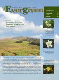
Boundary of Palakkad districts of Kerala (Fig.1.1). It is bounded byThrissur <str<strong>on</strong>g>and</str<strong>on</strong>g> Chavakkad Taluks of Thrissur district in the North,Mukundapuram <str<strong>on</strong>g>and</str<strong>on</strong>g> Kodungallur Taluks of Thrissur district in theSouth, Alathur <str<strong>on</strong>g>and</str<strong>on</strong>g> Chittor Taluks of Palakkad district in the East <str<strong>on</strong>g>and</str<strong>on</strong>g>the Arabian Sea in the West. Karuvannur River basin, c<strong>on</strong>stituting anarea of 1054 km 2 , lies in Southern Western Ghats <str<strong>on</strong>g>and</str<strong>on</strong>g> covers 32panchayats, 9 blocks <str<strong>on</strong>g>and</str<strong>on</strong>g> 2 districts. The river originates from theWestern Ghats <str<strong>on</strong>g>and</str<strong>on</strong>g> is fed by <str<strong>on</strong>g>its</str<strong>on</strong>g> two main tributaries, viz., the Manali <str<strong>on</strong>g>and</str<strong>on</strong>g>the Kurumali. The Manali river originates from P<strong>on</strong>mudi in the boundaryof Thrissur <str<strong>on</strong>g>and</str<strong>on</strong>g> Palakkad districts at an elevati<strong>on</strong> of + 928 m. TheChim<strong>on</strong>y <str<strong>on</strong>g>and</str<strong>on</strong>g> Muply, the two subtributaries of the Kurumali originatefrom Pundimudi at an elevati<strong>on</strong> of + 1116 m. This is <strong>on</strong>e of the major riverbasins with the actual utilizable water resources of 623 Mm 3 of which thenet utilizable surface <str<strong>on</strong>g>and</str<strong>on</strong>g> ground water resources are 519.8 Mm 3 <str<strong>on</strong>g>and</str<strong>on</strong>g>103.2 Mm 3 respectively. Karuvannur river has a drainage area of 1054km 2 , stream length 48 km, average m<strong>on</strong>so<strong>on</strong> flow of 1275 Mm 3 , averagelean flow 55 Mm 3 <str<strong>on</strong>g>and</str<strong>on</strong>g> total flow 1330 Mm 3 . (Rajagopalan <str<strong>on</strong>g>and</str<strong>on</strong>g> Sushanth,2001). The average rainfall in the low l<str<strong>on</strong>g>and</str<strong>on</strong>g> of the river basin wasestimated to be 2858 mm, the midl<str<strong>on</strong>g>and</str<strong>on</strong>g> 3011mm <str<strong>on</strong>g>and</str<strong>on</strong>g> the highl<str<strong>on</strong>g>and</str<strong>on</strong>g> 2851mm. About 60 per cent of the rainfall is received during south westm<strong>on</strong>so<strong>on</strong> period, 30 per cent from north east m<strong>on</strong>so<strong>on</strong> <str<strong>on</strong>g>and</str<strong>on</strong>g> 10 per cent inthe prem<strong>on</strong>so<strong>on</strong> period.Manali is <strong>on</strong>e of the important subwatershed systems in the river basin.This is also <strong>on</strong>e of the important forest areas of the river basin as well asthe district. Keeping the above facts in mind, Manali subwatershed wasselected for detailed study. Total area of this watershed is 274 km 2 <str<strong>on</strong>g>and</str<strong>on</strong>g>lies in Thrissur district of Kerala (Fig.1.1). It is spread over 13 villages,c<strong>on</strong>stituting a little over of 11 per cent of the total area of the district(3032 km 2 ). The utilizable annual surface water is 40.6 per cent of theavailable annual surface water <str<strong>on</strong>g>and</str<strong>on</strong>g> 25.5 per cent of the mean annualrainfall. The available annual surface water (mean runoff) is 62.8 per centof the mean annual rainfall (Rajagopalan <str<strong>on</strong>g>and</str<strong>on</strong>g> Sushanth, 2001).3
Fig.1.1 Locati<strong>on</strong> map of Karuvannur River Basin4
1.2 Ecological <str<strong>on</strong>g>and</str<strong>on</strong>g> ec<strong>on</strong>omic problems in the study areaMajor forest areas of the watershed are c<strong>on</strong>centrated at Peechi regi<strong>on</strong> ofPeechi Vazhani Wildlife Sanctuary which was established in 1958,c<strong>on</strong>stituting an area of 76.5 km 2 . Evergreen, semievergreen, moistdeciduous <str<strong>on</strong>g>and</str<strong>on</strong>g> scrub types of forests are the main vegetati<strong>on</strong> types ofwhich the first three account for 22, 17 <str<strong>on</strong>g>and</str<strong>on</strong>g> 28 per cent respectively.Owing to inadequate protecti<strong>on</strong>/c<strong>on</strong>servati<strong>on</strong> effort, this WildlifeSanctuary is characterized by high degradati<strong>on</strong> levels <str<strong>on</strong>g>and</str<strong>on</strong>g> low density ofwildlife. Of the total forest area, highly <str<strong>on</strong>g>and</str<strong>on</strong>g> moderately degraded areasaccount for 14 <str<strong>on</strong>g>and</str<strong>on</strong>g> 16 per cent respectively (Deepa, 2000). PeechiReservoir is located in the watershed which supplies major share of theirrigati<strong>on</strong> <str<strong>on</strong>g>and</str<strong>on</strong>g> drinking water in Thrissur district.Forest dwelling tribes were the early inhabitants of this area <str<strong>on</strong>g>and</str<strong>on</strong>g>depended up <strong>on</strong> collecti<strong>on</strong> of n<strong>on</strong>timber forest products (NTFPs) for theirlivelihood. Influx of settlers to this area can be traced back to early 1950’sat the time of c<strong>on</strong>structi<strong>on</strong> of Peechi dam across the Manali river <str<strong>on</strong>g>and</str<strong>on</strong>g>encroachment has been further accentuated in the subsequent years. Thesettlers are mostly agriculturists who cultivate a variety of crops such asvegetables, banana, rice, tapioca, cashew, rubber, etc. Ownership rightsof many settlers are undecided. People (tribal <str<strong>on</strong>g>and</str<strong>on</strong>g> other localcommunities) living immediately around the natural forests are highlydependent <strong>on</strong> the forests for agriculture, NTFPs, firewood, cattle grazing<str<strong>on</strong>g>and</str<strong>on</strong>g> small c<strong>on</strong>structi<strong>on</strong> needs, resulting in degradati<strong>on</strong> of forest areas. Inother words, the degradati<strong>on</strong> of forest was caused by biotic pressuressuch as illicit cutting, grazing, fire, etc. which are anthropogenic in origin.This has resulted in structural <str<strong>on</strong>g>and</str<strong>on</strong>g> other changes in the forest, includinginadequate regenerati<strong>on</strong> (Swarupan<str<strong>on</strong>g>and</str<strong>on</strong>g>an <str<strong>on</strong>g>and</str<strong>on</strong>g> Sasidharan, 1992).Our pilot survey indicated that there have been significant changes in thel<str<strong>on</strong>g>and</str<strong>on</strong>g>use which have had adverse effects <strong>on</strong> forest ecology, water yield, dryseas<strong>on</strong> flow, soil erosi<strong>on</strong>, stream sediment load, etc. <str<strong>on</strong>g>and</str<strong>on</strong>g> agriculturalproducti<strong>on</strong>. Originally, the Peechi Irrigati<strong>on</strong> Project was aimed at5
supplying irrigati<strong>on</strong> water to agricultural sector, including Kole l<str<strong>on</strong>g>and</str<strong>on</strong>g>s. Butdue to urbanisati<strong>on</strong> <str<strong>on</strong>g>and</str<strong>on</strong>g> the influence of the welltodo people in thedistrict, more water has been diverted for drinking purpose. This in turnhas brought about two major changes in the ec<strong>on</strong>omy. First, with thedecrease of supply through irrigati<strong>on</strong> canal, especially during summerseas<strong>on</strong>, the water tables in the well in the study area has g<strong>on</strong>e down,resulting in shortage of water. Sec<strong>on</strong>dly, in the absence of adequateirrigati<strong>on</strong> water supply, particularly in the mid <str<strong>on</strong>g>and</str<strong>on</strong>g> tail end regi<strong>on</strong>s of thecanals, the productivity of the crops have been declined which in turnadversely affected food security <str<strong>on</strong>g>and</str<strong>on</strong>g> income levels of the people.The area under crops in the watershed <str<strong>on</strong>g>and</str<strong>on</strong>g> also other irrigated areas inthe district have significantly declined over a period of time. The dem<str<strong>on</strong>g>and</str<strong>on</strong>g>of water for irrigati<strong>on</strong>, drinking, industrial <str<strong>on</strong>g>and</str<strong>on</strong>g> other comm<strong>on</strong> needs ismuch higher than the supply. There is no reliable informati<strong>on</strong> regardingdem<str<strong>on</strong>g>and</str<strong>on</strong>g>supply gap of water resources in Manali watershed. However, inthe Karuvannur River Basin, where this watershed is located, the deficit isexpected to be 22 Mm 3 in rabi seas<strong>on</strong> <str<strong>on</strong>g>and</str<strong>on</strong>g> 151 Mm 3 in summer seas<strong>on</strong>(Rajagopalan <str<strong>on</strong>g>and</str<strong>on</strong>g> Sushanth, 2001) indicating that water shortage is verysevere during summer. The drinking water supply from Peechi Reservoiris estimated to be 50.5 Mm 3 per day which meets a good part of the waterrequirements of the urban <str<strong>on</strong>g>and</str<strong>on</strong>g> semiurban areas of the district, but notthat of villages.The sustainability in the resource use is imperative for better livelihoodopportunities, envir<strong>on</strong>mental balance <str<strong>on</strong>g>and</str<strong>on</strong>g> rural development. Further, thebiophysical <str<strong>on</strong>g>and</str<strong>on</strong>g> socioec<strong>on</strong>omic linkages between the upl<str<strong>on</strong>g>and</str<strong>on</strong>g> <str<strong>on</strong>g>and</str<strong>on</strong>g>downstream areas of a watershed <str<strong>on</strong>g>and</str<strong>on</strong>g> <str<strong>on</strong>g>its</str<strong>on</strong>g> influence <strong>on</strong> overall ec<strong>on</strong>omicdevelopment have been widely accepted (James et al., 2000). The changesin the upl<str<strong>on</strong>g>and</str<strong>on</strong>g> areas have their own impact <strong>on</strong> downstream, as both areclosely interlinked. For instance, soil erosi<strong>on</strong> is a natural process but it getsaccelerated due to excessive anthropogenic activities <str<strong>on</strong>g>and</str<strong>on</strong>g> <str<strong>on</strong>g>its</str<strong>on</strong>g> implicati<strong>on</strong>sare mostly ec<strong>on</strong>omic, affecting welfare of the society (Kumar, 2000). Soil6
erosi<strong>on</strong> has both <strong>on</strong>site (direct) <str<strong>on</strong>g>and</str<strong>on</strong>g> offsite (indirect) impacts which affectproductivity of the upl<str<strong>on</strong>g>and</str<strong>on</strong>g> areas <str<strong>on</strong>g>and</str<strong>on</strong>g> ec<strong>on</strong>omic activities in thedownstream area. It also imposes ec<strong>on</strong>omic <str<strong>on</strong>g>and</str<strong>on</strong>g> envir<strong>on</strong>mental costs <strong>on</strong>people living in both the regi<strong>on</strong>s, which ultimately affect theirdevelopment. This requires a comprehensive envir<strong>on</strong>mental auditing ofsoil, water <str<strong>on</strong>g>and</str<strong>on</strong>g> producti<strong>on</strong> loss arising from l<str<strong>on</strong>g>and</str<strong>on</strong>g>use change in awatershed. This study is a modest attempt in this line.1.3 ObjectivesThe broad objective of this study is to examine l<str<strong>on</strong>g>and</str<strong>on</strong>g>use change <str<strong>on</strong>g>and</str<strong>on</strong>g> <str<strong>on</strong>g>its</str<strong>on</strong>g>effects <strong>on</strong> ecohydrology <str<strong>on</strong>g>and</str<strong>on</strong>g> socioec<strong>on</strong>omic c<strong>on</strong>diti<strong>on</strong>s of the people inthe study area. Specific attempts were made to:1. Study the nature <str<strong>on</strong>g>and</str<strong>on</strong>g> extent of l<str<strong>on</strong>g>and</str<strong>on</strong>g>use <str<strong>on</strong>g>and</str<strong>on</strong>g> cropping pattern changes<str<strong>on</strong>g>and</str<strong>on</strong>g> important socioec<strong>on</strong>omic drivers affecting it.2. Examine the effects of l<str<strong>on</strong>g>and</str<strong>on</strong>g>use <strong>on</strong> hydrology runoff, stream flow,ground water table, temperature <str<strong>on</strong>g>and</str<strong>on</strong>g> humidity in the watershed3. Analyze the effects of l<str<strong>on</strong>g>and</str<strong>on</strong>g>use/cropping pattern changes <strong>on</strong> vegetati<strong>on</strong>,sedimentati<strong>on</strong>, agricultural producti<strong>on</strong> <str<strong>on</strong>g>and</str<strong>on</strong>g> socioec<strong>on</strong>omic c<strong>on</strong>diti<strong>on</strong>sof the people4. Assess ec<strong>on</strong>omic value of water resource, surface water use pattern,pricing <str<strong>on</strong>g>and</str<strong>on</strong>g> use c<strong>on</strong>flict over water resources am<strong>on</strong>g different secti<strong>on</strong>sin the society5. Examine the linkages between ecological <str<strong>on</strong>g>and</str<strong>on</strong>g> socioec<strong>on</strong>omic systemsof the upl<str<strong>on</strong>g>and</str<strong>on</strong>g> <str<strong>on</strong>g>and</str<strong>on</strong>g> downstream areas of the watershed in determiningoverall development.7
Chapter 2METHODOLOGYBroadly, the study examines selected biophysical <str<strong>on</strong>g>and</str<strong>on</strong>g> socioec<strong>on</strong>omicaspects of the problem <str<strong>on</strong>g>and</str<strong>on</strong>g> integrates them to underst<str<strong>on</strong>g>and</str<strong>on</strong>g> theirimplicati<strong>on</strong>s in the development perspective. The methods employed tostudy major aspects of the problems are given below.2.1 Selecti<strong>on</strong> of micro watershedsA nested catchment approach has been followed in the selecti<strong>on</strong> of amicro watershed c<strong>on</strong>sidering the large area covered by the KaruvannurRiver Basin. The river basin, with several micro watersheds, has beendivided into upstream <str<strong>on</strong>g>and</str<strong>on</strong>g> downstream watershed, based <strong>on</strong> the elevati<strong>on</strong>data. One micro watershed, representative of the upstream catchment(Olakara) <str<strong>on</strong>g>and</str<strong>on</strong>g> another from the downstream catchment (Kavallur) havebeen chosen for detailed study.2.2 <str<strong>on</strong>g>L<str<strong>on</strong>g>and</str<strong>on</strong>g></str<strong>on</strong>g> use dynamicsSatellite data productsSatellite data products <strong>on</strong> 1:250,000 scale (hardcopy) <str<strong>on</strong>g>and</str<strong>on</strong>g> digital data ofIRS1C LISS III/IRS1D LISS III of January 1996 <str<strong>on</strong>g>and</str<strong>on</strong>g> IRS P6 (PAN+LISS3merged product) of January 2004 were used in the present study.Ancillary dataThe following ancillary data were used directly or indirectly for the studypurpose.i. Survey of India toposheets <strong>on</strong> 1:250,000 <str<strong>on</strong>g>and</str<strong>on</strong>g> 1:50,000 scales.ii. Forest type maps of India (Champi<strong>on</strong> <str<strong>on</strong>g>and</str<strong>on</strong>g> Seth, 1968)iii. Biogeographical map (Rodgers <str<strong>on</strong>g>and</str<strong>on</strong>g> Panwar, 1988)9
iv. Management maps/Stock maps of State Forest Departmentv. Forest Vegetati<strong>on</strong> maps <strong>on</strong> 1:250,000 scales <str<strong>on</strong>g>and</str<strong>on</strong>g> 1:50,000 scaleavailable with Forest Survey of India for Forest density layer <str<strong>on</strong>g>and</str<strong>on</strong>g>other relevant informati<strong>on</strong> as base details.2.3 Vegetati<strong>on</strong> classificati<strong>on</strong> schemeIn the present study, Level II vegetati<strong>on</strong> classificati<strong>on</strong> is attempted.Following classificati<strong>on</strong> scheme was adopted for stratificati<strong>on</strong>, usingRemote Sensing Digital data.Forest Vegetati<strong>on</strong>I. Forests1. Dominant phenological types1.1. Evergreen1.2. Semievergreen1.3. Moist deciduous1.4. Dry deciduous2. Gregarious types (single species dominated)2.1. Bamboo3. Local specific classes3.1. Mangrove3.2. Sholas3.3. Riverian3.4. Sacred groves4. Degradati<strong>on</strong> types4.1. Degraded forest stages (eg.1040 per cent tree density, signsof erosi<strong>on</strong> <str<strong>on</strong>g>and</str<strong>on</strong>g> compositi<strong>on</strong> are not c<strong>on</strong>firming with any of theabove types).10
II.III.ScrubsGrassl<str<strong>on</strong>g>and</str<strong>on</strong>g>sN<strong>on</strong>forest vegetati<strong>on</strong>IV.Major Wetl<str<strong>on</strong>g>and</str<strong>on</strong>g>sV. Plantati<strong>on</strong> (Tea/Coffee/Coc<strong>on</strong>ut gardens etc.)VI.AgricultureVII. Fallow/BarrenVIII. Water bodyIX.Settlement2.4 Digital classificati<strong>on</strong> of satellite dataPreprocessing: The raw digital data was enhanced using c<strong>on</strong>traststretching or ratio based techniques to facilitate better discriminati<strong>on</strong>during ground data collecti<strong>on</strong> or locating sample points.Rec<strong>on</strong>naissance survey: The rec<strong>on</strong>naissance survey was undertaken forgetting better acquaintance with the general nature of vegetati<strong>on</strong> of thearea. Major vegetati<strong>on</strong> types <str<strong>on</strong>g>and</str<strong>on</strong>g> few prime localities of characteristictypes were noted during rec<strong>on</strong>naissance survey. The variati<strong>on</strong>s <str<strong>on</strong>g>and</str<strong>on</strong>g> t<strong>on</strong>alpatterns were also observed <strong>on</strong> existing images/maps. Traversing al<strong>on</strong>gmajor drainage, roads, paths, etc. for ground truthing, existing literaturesurvey, <str<strong>on</strong>g>and</str<strong>on</strong>g> interacti<strong>on</strong> with forest officials were also made during fieldsurvey.2.5 Vegetati<strong>on</strong> characterizati<strong>on</strong> using satellite dataSatellite data in digital form were analysed to characterize the vegetati<strong>on</strong>using interactive digital analysis procedures. The preparati<strong>on</strong> ofvegetati<strong>on</strong> map assumes a critical step in the vegetati<strong>on</strong> characterizati<strong>on</strong>procedure.11
The study area falls in a single satellite scene. The scene wasgeometrically corrected with reference to Survey of India 1: 50,000 scaledToposheets. The Vegetati<strong>on</strong> classificati<strong>on</strong> was performed as per thescheme menti<strong>on</strong>ed earlier. The different scene was classified usingMaximum likelihood method. After complete classificati<strong>on</strong>, misclassifiedareas were checked <str<strong>on</strong>g>and</str<strong>on</strong>g> reclassified c<strong>on</strong>sidering small Area of Interest(AOI) or through interactive editing for improved accuracy. Finally theclassified subscenes were mosaiced <str<strong>on</strong>g>and</str<strong>on</strong>g> the edges were smoothened. Theapproach for l<str<strong>on</strong>g>and</str<strong>on</strong>g> cover mapping is as follows:Raw Satellite DataPreprocessingGeometric <str<strong>on</strong>g>and</str<strong>on</strong>g> radiometriccorrecti<strong>on</strong>Sun angle effectHaze removalRati<strong>on</strong>ingNDVI etc. Removal of (Histogram minimizati<strong>on</strong>discrepancies Dark object subtracti<strong>on</strong> etc.)Knowledge base Hybrid classificati<strong>on</strong> Ground truthingDigitally classified vegetati<strong>on</strong>/cover map2.6 Accuracy evaluati<strong>on</strong>The classificati<strong>on</strong> performance was evaluated by redundant training areas<str<strong>on</strong>g>and</str<strong>on</strong>g> field sample points based <strong>on</strong> the commissi<strong>on</strong> <str<strong>on</strong>g>and</str<strong>on</strong>g> omissi<strong>on</strong> errormatrix <str<strong>on</strong>g>and</str<strong>on</strong>g> hence overall classificati<strong>on</strong> accuracy was calculated. It shouldbe noted that overall classificati<strong>on</strong> accuracy is more than 85 per cent.12
Phytosociological data Collecti<strong>on</strong>Phytosociological analysis provides the real meaning to any biodiversity<str<strong>on</strong>g>and</str<strong>on</strong>g> vegetati<strong>on</strong> analysis by quantifying the structural parameters of thecommunities. The sampling principle was based <strong>on</strong> inventorying thehomogeneous strata identified by remote sensing data analysis. Accordingto the spectral signature variability in c<strong>on</strong>s<strong>on</strong>ance with the vegetati<strong>on</strong>type <str<strong>on</strong>g>and</str<strong>on</strong>g> orientati<strong>on</strong> of terrain, sample points were marked <strong>on</strong> 1: 50,000scale SOI toposheets in the study area. The plot size in the sample pointswas of 33 m x 33 m covering approximately an area of 0.1 hectare.Tax<strong>on</strong>omical census of each plot as well as menstruati<strong>on</strong> of individualwoody members qualifying as tree <str<strong>on</strong>g>and</str<strong>on</strong>g> shrub yielded the data essential forarriving structural status.Sampling strategyStratified r<str<strong>on</strong>g>and</str<strong>on</strong>g>om sampling with probability proporti<strong>on</strong> to the size (PPS)was adopted for analysing vegetati<strong>on</strong> compositi<strong>on</strong> of all the typesencountered. To sample an area of nearly 0.01 per cent of total area ofeach type, percentage sampling procedure was adopted. In view of thetime, m<strong>on</strong>ey <str<strong>on</strong>g>and</str<strong>on</strong>g> availability of other resources, optimum number ofsample points has been taken up, covering all vegetati<strong>on</strong> type, in differentdensity/disturbance regimes.For each vegetati<strong>on</strong> type, the size of the quadrat was determined through‘SpeciesArea curve method’ (Muller – Dombois <str<strong>on</strong>g>and</str<strong>on</strong>g> Ellenberg, 1978). Theplot size was restricted to 0.1 ha. (32 m x 32 m). A minimum of 810quadrats were analysed for each vegetati<strong>on</strong> type.Marking locati<strong>on</strong> of sample plotsEach sample site was located <strong>on</strong> survey of India toposheets. Exactl<strong>on</strong>gitude <str<strong>on</strong>g>and</str<strong>on</strong>g> latitude <str<strong>on</strong>g>and</str<strong>on</strong>g> locati<strong>on</strong> height (msl) were noted down usingGlobal Positi<strong>on</strong> System (Garmin III plus <str<strong>on</strong>g>and</str<strong>on</strong>g> Trimble GeoXT).13
Creati<strong>on</strong> of watershed boundaries <str<strong>on</strong>g>and</str<strong>on</strong>g> masksThe precise watershed boundaries as obtained from Survey of Indiatoposheets were used <str<strong>on</strong>g>and</str<strong>on</strong>g> the bit map was created to use them aswatershed mask. It was ensured that the SOI watershed boundaries areproperly registered <strong>on</strong> the geometrically corrected image <str<strong>on</strong>g>and</str<strong>on</strong>g> georeferencedmap.Plot method <str<strong>on</strong>g>and</str<strong>on</strong>g> enumerati<strong>on</strong>At each sample plot, complete enumerati<strong>on</strong>s of species were d<strong>on</strong>e. Thecircumferences at breast height (cbh) or 1.3 m above ground level, of alltree species were recorded. The individuals with cbh >30 cm werec<strong>on</strong>sidered as tree <str<strong>on</strong>g>and</str<strong>on</strong>g> with >17 cm <str<strong>on</strong>g>and</str<strong>on</strong>g>
Total number of quadrats in which species occurredFrequency = _______________________________________________ X 100Total number of quadrats studiedTotal number of individuals of the speciesDensity = __________________________________________ X 100(per quadrat) Total number of quadrats studiedTotal number of individuals of species occurringAbundance = _______________________________________________ X 100Total number of quadrats in which species occurredFrequency of a speciesRelative frequency = __________________________ X 100Sum of frequency of all speciesRelative density = Density of a species___________________________ X 100Sum of density of all speciesRelative dominance =Total st<str<strong>on</strong>g>and</str<strong>on</strong>g> basal cover of species___________________________________ X 100Total st<str<strong>on</strong>g>and</str<strong>on</strong>g> basal cover of all the speciesBasal cover = (cbh) 2______4 IISum of basal cover of individual plants of a species will yield total st<str<strong>on</strong>g>and</str<strong>on</strong>g>basal cover of that species.Importance Value Index (IVI) = Relative Frequency + Relative Density +Relative DominancePlant diversityThe plants were enumerated by line transect method. Three enumerati<strong>on</strong>sin the m<strong>on</strong>ths of January, March <str<strong>on</strong>g>and</str<strong>on</strong>g> October were carried out to have arepresentati<strong>on</strong> of plants occurring in different seas<strong>on</strong>s of the year. Plantswere mostly identified in the field during enumerati<strong>on</strong>. Species which15
could not be identified in the field were brought to the Institute <str<strong>on</strong>g>and</str<strong>on</strong>g>identified with the literature (Sasidharan <str<strong>on</strong>g>and</str<strong>on</strong>g> Sivarajan, 1996) <str<strong>on</strong>g>and</str<strong>on</strong>g> bycomparing with authentic herbarium specimens in the Kerala ForestResearch Institute Herbarium.2.7 Hydro meteorological observati<strong>on</strong>sHistorical data <strong>on</strong> rainfall <str<strong>on</strong>g>and</str<strong>on</strong>g> stream flow data for the last few years,sometimes as early as 1963 were collected from the HydrologyDepartment, Government of Kerala.Rainfall distributi<strong>on</strong> during study periodTipping bucket rain gauges (Onset Computer Corporati<strong>on</strong>, USA) wereinstalled <str<strong>on</strong>g>and</str<strong>on</strong>g> daily data from January 2005 till December 2006 wererecorded at both watersheds of Olakara <str<strong>on</strong>g>and</str<strong>on</strong>g> Kavallur.Stream flow measurementThree streams were identified in both the watersheds for measurement.Daily measurements for the flow were taken. Flow measurement wastaken using velocity float method. The depth of the flow through the outletwas measured twice a day at 8.00 a.m. <str<strong>on</strong>g>and</str<strong>on</strong>g> 2.30 p.m.Velocity float methodIn the velocity float method, discharge rate was computed using theformula,Q=AV= (bd) L/twhere, Q = Discharge rate (m 3 /sec)A = Area of cross secti<strong>on</strong> of flow (m 2 )V = Velocity of flow (m/sec)d = Depth of flow (m)b = Width of flow (m)t = Time taken by the float (sec) to travel specified distance in m16
Depth of flow <str<strong>on</strong>g>and</str<strong>on</strong>g> time taken by the float to reach the length were notedeveryday. Velocity was calculated. By multiplying velocity with area of flowthe discharge was measured.At Olakara, three streams were m<strong>on</strong>itored in the micro watershed forstream flow. All the three streams were flowing through forested areas. AtKavallur also, three streams were m<strong>on</strong>itored:Stream 1 Originating <str<strong>on</strong>g>and</str<strong>on</strong>g> flowing through a felled Eucalyptus plantati<strong>on</strong>Stream 2 Originating from a forest <str<strong>on</strong>g>and</str<strong>on</strong>g> flowing through plantati<strong>on</strong> whichis planted under social forestry projectStream 3 Originating <str<strong>on</strong>g>and</str<strong>on</strong>g> flowing through agricultural l<str<strong>on</strong>g>and</str<strong>on</strong>g>2.8 Water table fluctuati<strong>on</strong> studiesTen wells from each micro watershed were selected for the water tablefluctuati<strong>on</strong> studies. Observati<strong>on</strong> regarding the water level was taken at 15days interval. The depth of water table was taken as the depth from theground level to top of water level in the well. Fluctuati<strong>on</strong>s were calculated<str<strong>on</strong>g>and</str<strong>on</strong>g> depicted in the graphical form.Relative humidity <str<strong>on</strong>g>and</str<strong>on</strong>g> temperatureData loggers (Gemini Tiny tag data loggers, UK) for measuring dailytemperature <str<strong>on</strong>g>and</str<strong>on</strong>g> relative humidity (with thermistor <str<strong>on</strong>g>and</str<strong>on</strong>g> humicap sensors)were installed at both watersheds. Hourly data were recorded.Ground water table observati<strong>on</strong>Open dug wells are basic groundwater source for both sites. Based <strong>on</strong> thephysical survey carried out, 11 open wells were selected for ground watertable studies from Kavallur <str<strong>on</strong>g>and</str<strong>on</strong>g> 8 from Olakara. Kavallur area comprisesof paddy fields, coc<strong>on</strong>ut, banana, vegetables <str<strong>on</strong>g>and</str<strong>on</strong>g> rubber plantati<strong>on</strong>s. Allthe wells selected in Olakara were located within the forest area. Datawere collected fortnightly using a measuring tape.17
Soil physicochemical propertiesTwentyfive plots of 33 m x 33 m size were laid out in the experimentalarea at Olakara. In each plot, three soil p<str<strong>on</strong>g>its</str<strong>on</strong>g> of 60 cm x 60 cm x 30 cmdimensi<strong>on</strong>s were taken <str<strong>on</strong>g>and</str<strong>on</strong>g> soils collected from 020 cm, 2040 cm <str<strong>on</strong>g>and</str<strong>on</strong>g>4060 cm depths. The soils from three p<str<strong>on</strong>g>its</str<strong>on</strong>g> of the same depth were mixed<str<strong>on</strong>g>and</str<strong>on</strong>g> made into a composite sample. The samples were air dried <str<strong>on</strong>g>and</str<strong>on</strong>g>processed for determinati<strong>on</strong> of gravel, particlesize separates, bulkdensity, maximum water holding capacity, pH <str<strong>on</strong>g>and</str<strong>on</strong>g> organic carb<strong>on</strong>.In six plots at Olakara, locally fabricated sediment collectors wereinstalled. The sediments were collected at periodic intervals in July,August <str<strong>on</strong>g>and</str<strong>on</strong>g> October 2005 <str<strong>on</strong>g>and</str<strong>on</strong>g> June, August <str<strong>on</strong>g>and</str<strong>on</strong>g> September 2006. Thecollected sediments were quantified <str<strong>on</strong>g>and</str<strong>on</strong>g> the nutrient c<strong>on</strong>tents (Nitrogen,Phosphorus <str<strong>on</strong>g>and</str<strong>on</strong>g> Potassium) were found out. Attempts were also made toassess sediment yield in the Kavallur area. Unfortunately no data couldbe collected as the sediment collectors installed in the field weredestroyed.2.9 Socioec<strong>on</strong>omic aspectsSocioec<strong>on</strong>omicsThe socioec<strong>on</strong>omic part of the study is based <strong>on</strong> both primary <str<strong>on</strong>g>and</str<strong>on</strong>g>sec<strong>on</strong>dary data. The primary data were gathered from a sample ofhouseholds. The study area was spread over 13 villages (Marakkal,Vaniyampara, Chuvannmannu, Pattikkad, Kannara, Peechi,Maniyankinaru, Olakara, Kavallur, Puttur, Nadathara, Manamangalam,<str<strong>on</strong>g>and</str<strong>on</strong>g> Pudukkad) in Trichur taluk of which six villages, that is, three eachfrom upl<str<strong>on</strong>g>and</str<strong>on</strong>g> <str<strong>on</strong>g>and</str<strong>on</strong>g> downstream areas were selected at r<str<strong>on</strong>g>and</str<strong>on</strong>g>om for primarydata collecti<strong>on</strong>. Data were collected from 100 households located in theselected villages. Primary data were gathered from 100 farmers in theupl<str<strong>on</strong>g>and</str<strong>on</strong>g> <str<strong>on</strong>g>and</str<strong>on</strong>g> downstream areas using multistage stratified r<str<strong>on</strong>g>and</str<strong>on</strong>g>omsampling technique. The time series data relating to change in the18
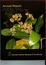
ec<strong>on</strong>omic variables such as producti<strong>on</strong>, price <str<strong>on</strong>g>and</str<strong>on</strong>g> cropping pattern, etc.were gathered from sec<strong>on</strong>dary sources viz., publicati<strong>on</strong>s of the StatePlanning Board, <str<strong>on</strong>g>and</str<strong>on</strong>g> Kerala State <str<strong>on</strong>g>L<str<strong>on</strong>g>and</str<strong>on</strong>g></str<strong>on</strong>g> <str<strong>on</strong>g>Use</str<strong>on</strong>g> Board. Historical data weregathered from ageold people in the study area.2.10 Ec<strong>on</strong>omic valuati<strong>on</strong> of water resourcesIn the study area, the reservoir is used for supplying water for irrigati<strong>on</strong><str<strong>on</strong>g>and</str<strong>on</strong>g> drinking purposes, fishing, ecotourism <str<strong>on</strong>g>and</str<strong>on</strong>g> educati<strong>on</strong> <str<strong>on</strong>g>and</str<strong>on</strong>g> research.It also gives a number of functi<strong>on</strong>al benef<str<strong>on</strong>g>its</str<strong>on</strong>g> such as increasingagricultural productivity, soil c<strong>on</strong>servati<strong>on</strong>, recharging of ground water<str<strong>on</strong>g>and</str<strong>on</strong>g> regulati<strong>on</strong> of stream flows. Thus, value of the water resources mightbe much higher than <strong>on</strong>e generally perceives. An attempt was made toestimate market <str<strong>on</strong>g>and</str<strong>on</strong>g> n<strong>on</strong> market benef<str<strong>on</strong>g>its</str<strong>on</strong>g> of the water resources in thePeechi Reservoir in the total ec<strong>on</strong>omic value framework.Total ec<strong>on</strong>omic value of Peechiwetl<str<strong>on</strong>g>and</str<strong>on</strong>g>s was undertaken using thest<str<strong>on</strong>g>and</str<strong>on</strong>g>ard tools for valuati<strong>on</strong> of ecosystem. Munasinghe (1992) hasclassified of the major categories of value assigned to nature (Fig.2.1).This was used as an analytical tool to determine the main valuesassociated with the functi<strong>on</strong>s of the wetl<str<strong>on</strong>g>and</str<strong>on</strong>g>s <str<strong>on</strong>g>and</str<strong>on</strong>g> to identify suitablevaluati<strong>on</strong> tools to assess their m<strong>on</strong>etary value. Munasinghe (1992) dividedthe total ec<strong>on</strong>omic value of nature into use <str<strong>on</strong>g>and</str<strong>on</strong>g> n<strong>on</strong>use values. The usevalues are divided into the direct <str<strong>on</strong>g>and</str<strong>on</strong>g> indirect use values <str<strong>on</strong>g>and</str<strong>on</strong>g> opti<strong>on</strong>values. The n<strong>on</strong>use values are divided into existence <str<strong>on</strong>g>and</str<strong>on</strong>g> bequest values.The TEV is embedded in the total value c<strong>on</strong>cept, which is detailed in thefollowing secti<strong>on</strong>.Total valueThe total value (TV) of an ecosystem is the sum of two comp<strong>on</strong>ents: aprimary value (PV) <str<strong>on</strong>g>and</str<strong>on</strong>g> a sec<strong>on</strong>dary value (SV).TV = PV + SV (1)19
Primary valueThe Primary value (PV) or 'glue' value or 'intrinsic' value is not associatedwith the ecosystem's use, but is bey<strong>on</strong>d <str<strong>on</strong>g>its</str<strong>on</strong>g> value to humans (Turner etal., 1994). The PV is rather perceived as a n<strong>on</strong> anthropocentric or'ecocentric' value which is inherent to the ecosystem's self organizingcapacity, <str<strong>on</strong>g>and</str<strong>on</strong>g> hence to <str<strong>on</strong>g>its</str<strong>on</strong>g> existence <str<strong>on</strong>g>and</str<strong>on</strong>g> c<strong>on</strong>tinuity, independently ofhuman preferences, <str<strong>on</strong>g>and</str<strong>on</strong>g> irrespective of human desires or will.Total Ec<strong>on</strong>omic Value<str<strong>on</strong>g>Use</str<strong>on</strong>g> valuesN<strong>on</strong> use valuesDirect usevaluesIndirect usevaluesOpti<strong>on</strong>valuesBequestvaluesExistencevaluesOutputs thatcan bec<strong>on</strong>sumeddirectlyFuncti<strong>on</strong>albenef<str<strong>on</strong>g>its</str<strong>on</strong>g>Future direct<str<strong>on</strong>g>and</str<strong>on</strong>g> indirectuse valuesValues ofleaving use<str<strong>on</strong>g>and</str<strong>on</strong>g> n<strong>on</strong> usevalues foroffspringValue fromknowledgeofc<strong>on</strong>tinuedexistence,based <strong>on</strong>e.g. moralValues offuncti<strong>on</strong>srelated to:¨ Food¨ Biomass¨ Recreati<strong>on</strong>¨ HealthValues offuncti<strong>on</strong>srelated to:¨Ecologicalfuncti<strong>on</strong>s¨Floodc<strong>on</strong>trol¨Stormprotecti<strong>on</strong>Values offuncti<strong>on</strong>srelated to:¨ Biodiversity¨ C<strong>on</strong>servedhabitatsValues offuncti<strong>on</strong>srelated to:¨ Habitats¨ Irreversible changesValues offuncti<strong>on</strong>srelated to:¨ Habitats¨ EndangeredspeciesFig. 2.1 Classificati<strong>on</strong> of total ec<strong>on</strong>omic value, (Source: Munasinghe, 1992)20
Sec<strong>on</strong>dary valueThe sec<strong>on</strong>dary value (SV) or 'instrumental' value or 'ec<strong>on</strong>omic' value israther an anthropocentric, utilitarian value, which fully relies <strong>on</strong> humanselfinterest, <str<strong>on</strong>g>and</str<strong>on</strong>g> is derived <strong>on</strong>ly from individual preferences. It is equal tothe total worth of the ecosystem's goods <str<strong>on</strong>g>and</str<strong>on</strong>g> services provided for theindividual. It is the comm<strong>on</strong>ly known c<strong>on</strong>cept developed by the ec<strong>on</strong>omicscience (Pearce, 1999), called total ec<strong>on</strong>omic value (TEV), <str<strong>on</strong>g>and</str<strong>on</strong>g> c<strong>on</strong>sistingof use values (UV) which include direct use values (DUV), indirect usevalues (IUV) <str<strong>on</strong>g>and</str<strong>on</strong>g> opti<strong>on</strong> values (OV) <str<strong>on</strong>g>and</str<strong>on</strong>g> n<strong>on</strong>use values (NUV) whichinclude existence value (EV) <str<strong>on</strong>g>and</str<strong>on</strong>g> bequest value (BV).SV = UV + NUV (2)UV = DUV + IUV (3)NUV = EV + BV (4)Combining equati<strong>on</strong>s (3) <str<strong>on</strong>g>and</str<strong>on</strong>g> (4); EV = (DUV+IUV+OV)+(EV+BV) (5)<str<strong>on</strong>g>Use</str<strong>on</strong>g> valuesAccording to the classificati<strong>on</strong> adopted by Turner et al. (1994), the usevalues (UV) are disaggregated into direct use values (DUV), indirect usevalues (IUV) <str<strong>on</strong>g>and</str<strong>on</strong>g> opti<strong>on</strong> values (OV).Direct use valueDirect c<strong>on</strong>sumptive useThe direct use value (DUV) is broadly determined by the producti<strong>on</strong> ofmeasurable <str<strong>on</strong>g>and</str<strong>on</strong>g> merchantable (or at least potentially merchantable)outputs. For wetl<str<strong>on</strong>g>and</str<strong>on</strong>g> ecosystems, DUV is subdivided into c<strong>on</strong>sumptivevalues (CV), <str<strong>on</strong>g>and</str<strong>on</strong>g> n<strong>on</strong>c<strong>on</strong>sumptive values (NCV), such as recreati<strong>on</strong>,sightseeing, spiritual use. DUV is practically equal to the net incomegenerated from the ecosystem. For assessing the value of tangible benef<str<strong>on</strong>g>its</str<strong>on</strong>g>viz.,, fish, the following formula was adopted.21
where,nDUV = å ( P i Q i - C i )(6)iP i is the price of product i ,Q i is the amount of product i , being harvested, <str<strong>on</strong>g>and</str<strong>on</strong>g>C i is the cost involved in the harvesting of product i .Direct n<strong>on</strong>c<strong>on</strong>sumptive useThe recreati<strong>on</strong> benef<str<strong>on</strong>g>its</str<strong>on</strong>g>/tourism benef<str<strong>on</strong>g>its</str<strong>on</strong>g> were estimated using travel costmethod (TCM). Travel cost method was applied in the study area forestimating the c<strong>on</strong>sumer surplus of the visitors. The dam is under thec<strong>on</strong>trol of Irrigati<strong>on</strong> Department <str<strong>on</strong>g>and</str<strong>on</strong>g> prior permissi<strong>on</strong> is not required forthe same. A nominal entrance fee of Rs 2/ is charged for the visitors ofdam.The Claws<strong>on</strong> <str<strong>on</strong>g>and</str<strong>on</strong>g> Knetsch (1966); TCM dem<str<strong>on</strong>g>and</str<strong>on</strong>g> functi<strong>on</strong> is of the form:V i = f (P i , X)where,Vi = Visitati<strong>on</strong> rate of i th populati<strong>on</strong>P i = Cost of visiting the site from z<strong>on</strong>e 1X = Vector of socio ec<strong>on</strong>omic variables affecting travel costdem<str<strong>on</strong>g>and</str<strong>on</strong>g> curveThe individual travel cost method was applied in the study to estimate thedem<str<strong>on</strong>g>and</str<strong>on</strong>g> functi<strong>on</strong>. The study adopted a semi log functi<strong>on</strong> to estimate thedem<str<strong>on</strong>g>and</str<strong>on</strong>g> functi<strong>on</strong>. The c<strong>on</strong>sumer surpluses were estimated from thecoefficients obtained from the dem<str<strong>on</strong>g>and</str<strong>on</strong>g> functi<strong>on</strong> (Hangley, 1989).The estimated dem<str<strong>on</strong>g>and</str<strong>on</strong>g> functi<strong>on</strong> is of the form;V = f (X1, X2, ….X8)where,V =X1 =Number of vis<str<strong>on</strong>g>its</str<strong>on</strong>g> by each visitorResidence of the resp<strong>on</strong>dent (local=1, 0 otherwise)22
X 2 = Educati<strong>on</strong> (dummy variable)X 3 = Willingness to pay (Rs.)X 4 = Income (Rs. year 1 )X 5 = Visiting day (weekend=1, weekdays= 0)X 6 = Opportunity cost of time (income corrected for hoursspent at the site (Rs.)X7 =X8 =X 9 =X10 =Travel cost (expenses incurred <strong>on</strong> travel Rs/pers<strong>on</strong>)Distance traveled (km)Infrastructure (dummy variable; improve presentc<strong>on</strong>diti<strong>on</strong>=1; 0 otherwise)Local travel cost (expenses at the site in Rs.)Three basic steps are involved in travel cost models. First, it is necessaryto undertake a survey of a sample of individuals visiting the site todetermine their costs incurred in visiting the site. These costs includetravel time, any financial expenditure involved in getting to <str<strong>on</strong>g>and</str<strong>on</strong>g> from thesite, al<strong>on</strong>g with entrance (or parking) fees. In additi<strong>on</strong>, informati<strong>on</strong> <strong>on</strong> theplace of origin for the journey, <str<strong>on</strong>g>and</str<strong>on</strong>g> basic socioec<strong>on</strong>omic factors such asincome <str<strong>on</strong>g>and</str<strong>on</strong>g> educati<strong>on</strong> of the individual is required. The resulting data ismanipulated to derive a dem<str<strong>on</strong>g>and</str<strong>on</strong>g> equati<strong>on</strong> for the site. This relates thenumber of vis<str<strong>on</strong>g>its</str<strong>on</strong>g> to the site to the costs per visit. The third step is toderive the value of a change in envir<strong>on</strong>mental c<strong>on</strong>diti<strong>on</strong>s. For this, it isnecessary to determine how willingness to pay for what the site has tooffer alters with changes in the features of the site. The domestic touristsfrequented the site while foreigners visited very rarely or occasi<strong>on</strong>ally.Hence dem<str<strong>on</strong>g>and</str<strong>on</strong>g> functi<strong>on</strong> was estimated for <strong>on</strong>ly domestic tourists.Indirect use valuesThe indirect use values (IUV) are derived basically from the functi<strong>on</strong>alservices provided by the ecosystem to support current producti<strong>on</strong> <str<strong>on</strong>g>and</str<strong>on</strong>g>c<strong>on</strong>sumpti<strong>on</strong> (eg. hydrological cycle stability, natural filtrati<strong>on</strong> of pollutedwater, climate regulati<strong>on</strong>, recycling of nutrients, biodiversity, etc.).23
Opti<strong>on</strong> valuesC<strong>on</strong>trary to direct <str<strong>on</strong>g>and</str<strong>on</strong>g> indirect use values which refer to (potential)effective use of the ecosystem's goods <str<strong>on</strong>g>and</str<strong>on</strong>g> services by humans at present,the opti<strong>on</strong> value (OV) refers to opti<strong>on</strong> of a potential use of these goods <str<strong>on</strong>g>and</str<strong>on</strong>g>services, by people themselves or by future generati<strong>on</strong>s. In the c<strong>on</strong>text ofOV, people preserve ecosystem functi<strong>on</strong>s for possible use in the future, evenif others will use them.N<strong>on</strong>use valuesThe c<strong>on</strong>cept of n<strong>on</strong>use values (NUVs) is more complicated to define <str<strong>on</strong>g>and</str<strong>on</strong>g>measure; they are also referred to as 'passive' use values; they are notassociated with actual ecosystem’s use, or even with the alternative to usea good or service. According to the classificati<strong>on</strong> adopted by Turner et al.(1994), NUVs are disaggregated into existence value (EV) <str<strong>on</strong>g>and</str<strong>on</strong>g> bequestvalue (BV).Existence value <str<strong>on</strong>g>and</str<strong>on</strong>g> bequest valueThe existence value (EV) is the satisfacti<strong>on</strong> value derived by individualsfrom the pure fact that an ecosystem <str<strong>on</strong>g>and</str<strong>on</strong>g>/or <str<strong>on</strong>g>its</str<strong>on</strong>g> c<strong>on</strong>stituents exist, fortheir own, regardless of necessarily seeing it or having any intenti<strong>on</strong> ofusing it directly (Turner et al., 1994). The bequest value (BV) is perceivedas the moral value people derive from knowing that an ecosystem <str<strong>on</strong>g>and</str<strong>on</strong>g>/or<str<strong>on</strong>g>its</str<strong>on</strong>g> c<strong>on</strong>stituents will be passed <strong>on</strong> to future generati<strong>on</strong>s to enjoy it.C<strong>on</strong>tingent valuati<strong>on</strong> methodPrimarily, c<strong>on</strong>tingent valuati<strong>on</strong> method was used to know the willingnessto pay. C<strong>on</strong>tingent Valuati<strong>on</strong> (CV) surveys directly ask people what theyare willing to pay for something they value or are willing to receive incompensati<strong>on</strong> for tolerating a cost. Pers<strong>on</strong>al valuati<strong>on</strong>s for increase ordecrease in the quantity of some goods based <strong>on</strong> a hypothetical marketare undertaken. The aim is to elicit valuati<strong>on</strong>s or bids, which are close to24
what would be revealed if an actual market existed. CV employs aquesti<strong>on</strong>naire format where resp<strong>on</strong>dents are asked how much they wouldbe willing to pay or willing to accept compensati<strong>on</strong> for a specified gain orloss of a given good or service. Ec<strong>on</strong>omic value estimates yielded by CVsurveys are ‘c<strong>on</strong>tingent’ up<strong>on</strong> the hypothetical market situati<strong>on</strong> that ispresented to resp<strong>on</strong>dents <str<strong>on</strong>g>and</str<strong>on</strong>g> allows them to trade off gains <str<strong>on</strong>g>and</str<strong>on</strong>g> lossesagainst m<strong>on</strong>ey. WTP/WTA questi<strong>on</strong>s may be asked in a number of ways,including openended, where the resp<strong>on</strong>dent states their maximumWTP/WTA, <str<strong>on</strong>g>and</str<strong>on</strong>g> dichotomous choice, where the resp<strong>on</strong>dent is required toanswer yes or no to a ‘bid’.Simple CVM exercises can be based <strong>on</strong> the “open ended” elicitati<strong>on</strong>formats, where the individual is simply asked to state his/her maximumWTP or minimum WTA for a given envir<strong>on</strong>mental change. However, thisapproach becomes biased when the resp<strong>on</strong>dent state a WTP/WTA lower orhigher than the true <strong>on</strong>e in order to influence the decisi<strong>on</strong> making processfor the sake of his own profit. To avoid the drawbacks of open – endedformat, an iterative technique called the “bidding game” is used. In thistechnique the resp<strong>on</strong>dent is asked whether he accepts to pay a givenamount of m<strong>on</strong>ey. If he refuses, the proposed amount is reduced(increased) by a given percentage (say 10%). The procedure is repeateduntil the resp<strong>on</strong>dent answers “yes”. The penultimate amount is taken ashis maximum WTP (minimum WTA) for obtaining (to give up) theenvir<strong>on</strong>mental improvement. If the individual accepts the proposedamount is increased (decreased) of say 10 per cent. The procedurec<strong>on</strong>tinues until the individual answers “no”. Here also the last amountproposed is taken as his maximum WTP (minimum WTA) for obtaining (togive up) the envir<strong>on</strong>mental improvement. Some of the data relating topricing of water have been drawn from studies carried out in the studyarea recently (Sreelakshmi, 2005)The stakeholders of Peechi wetl<str<strong>on</strong>g>and</str<strong>on</strong>g>s were classified into three, viz.,drinking water users, irrigati<strong>on</strong> users <str<strong>on</strong>g>and</str<strong>on</strong>g> fishermen for the purpose ofthe study. Data were gathered from 120 drinking water users, 27025
irrigati<strong>on</strong> users <str<strong>on</strong>g>and</str<strong>on</strong>g> 50 fishermen who catch fish from Peechi reservoir.Primary data collected from the farmers <str<strong>on</strong>g>and</str<strong>on</strong>g> those who use drinking waterwere used to study water use efficiency <str<strong>on</strong>g>and</str<strong>on</strong>g> use c<strong>on</strong>flict. Data collectedfrom 500 tourists were used for estimati<strong>on</strong> of recreati<strong>on</strong> value.The study also made use of relevant sec<strong>on</strong>dary data collected from the 20respective village offices, forest range offices, Irrigati<strong>on</strong> Department <str<strong>on</strong>g>and</str<strong>on</strong>g>office of the Kerala Water Authority.26
Chapter 3LAND USE AND CROPPING PATTERN CHANGESThe extent, magnitude <str<strong>on</strong>g>and</str<strong>on</strong>g> intensity of l<str<strong>on</strong>g>and</str<strong>on</strong>g> use <str<strong>on</strong>g>and</str<strong>on</strong>g> <str<strong>on</strong>g>its</str<strong>on</strong>g> resultant changesin the agricultural sector are discussed in this secti<strong>on</strong>. This chapter isorganized <str<strong>on</strong>g>and</str<strong>on</strong>g> presented under three headings viz., l<str<strong>on</strong>g>and</str<strong>on</strong>g> use change,cropping pattern change <str<strong>on</strong>g>and</str<strong>on</strong>g> socioec<strong>on</strong>omic drivers of l<str<strong>on</strong>g>and</str<strong>on</strong>g> use <str<strong>on</strong>g>and</str<strong>on</strong>g>cropping pattern changes.3.1 <str<strong>on</strong>g>L<str<strong>on</strong>g>and</str<strong>on</strong>g></str<strong>on</strong>g> use change<str<strong>on</strong>g>L<str<strong>on</strong>g>and</str<strong>on</strong>g></str<strong>on</strong>g> is defined as an area where all human activities are c<strong>on</strong>ducted <str<strong>on</strong>g>and</str<strong>on</strong>g>it is also the source of the materials needed for this anthropogenicc<strong>on</strong>duct (Briassoulis, 2000). Human use of l<str<strong>on</strong>g>and</str<strong>on</strong>g> resources gives rise tol<str<strong>on</strong>g>and</str<strong>on</strong>g> use <str<strong>on</strong>g>and</str<strong>on</strong>g> generally, the two broad sets of dynamic factors/forces,which influence the l<str<strong>on</strong>g>and</str<strong>on</strong>g> use, are human needs <str<strong>on</strong>g>and</str<strong>on</strong>g> envir<strong>on</strong>mentalfeatures <str<strong>on</strong>g>and</str<strong>on</strong>g> processes. The operati<strong>on</strong>s of these forces are c<strong>on</strong>tinuousresulting in frequent changes in the l<str<strong>on</strong>g>and</str<strong>on</strong>g> uses <str<strong>on</strong>g>and</str<strong>on</strong>g> the magnitude of l<str<strong>on</strong>g>and</str<strong>on</strong>g>use change varies with the time period being examined as well as with thegeographical area. These changes have at times been beneficial <str<strong>on</strong>g>and</str<strong>on</strong>g> attimes caused detrimental impacts or effects. The latter is the chief causeof c<strong>on</strong>cern, as they impinge variously <strong>on</strong> human wellbeing <str<strong>on</strong>g>and</str<strong>on</strong>g> welfare(Meyer <str<strong>on</strong>g>and</str<strong>on</strong>g> Turner, 1994).The terms l<str<strong>on</strong>g>and</str<strong>on</strong>g> use <str<strong>on</strong>g>and</str<strong>on</strong>g> l<str<strong>on</strong>g>and</str<strong>on</strong>g> cover, though not strictly syn<strong>on</strong>ymous, havebeen used interchangeably worldwide. Therefore, an underst<str<strong>on</strong>g>and</str<strong>on</strong>g>ing ofthe different l<str<strong>on</strong>g>and</str<strong>on</strong>g> related terms assumes significance while taking up anystudy <strong>on</strong> l<str<strong>on</strong>g>and</str<strong>on</strong>g> use change. <str<strong>on</strong>g>L<str<strong>on</strong>g>and</str<strong>on</strong>g></str<strong>on</strong>g> cover is the biophysical state of earth’ssurface <str<strong>on</strong>g>and</str<strong>on</strong>g> the immediate subsurface (Turner et al., 1995). Originally,the term referred to the type of vegetati<strong>on</strong> that covered the l<str<strong>on</strong>g>and</str<strong>on</strong>g> surface,but has broadened eventually to include human structures, such asbuildings or pavements, <str<strong>on</strong>g>and</str<strong>on</strong>g> other aspects of the physical envir<strong>on</strong>ment(Moser, 1996). The l<str<strong>on</strong>g>and</str<strong>on</strong>g> use involves both the manner in which thebiophysical attributes of the l<str<strong>on</strong>g>and</str<strong>on</strong>g> are manipulated <str<strong>on</strong>g>and</str<strong>on</strong>g> the intent27
underlying that manipulati<strong>on</strong> the purpose for which the l<str<strong>on</strong>g>and</str<strong>on</strong>g> is used(Turner et al., 1994). In other words, l<str<strong>on</strong>g>and</str<strong>on</strong>g> use denotes the humanemployment of l<str<strong>on</strong>g>and</str<strong>on</strong>g> (Turner et al., 1995). In this study, the words l<str<strong>on</strong>g>and</str<strong>on</strong>g> cover<str<strong>on</strong>g>and</str<strong>on</strong>g> l<str<strong>on</strong>g>and</str<strong>on</strong>g> use changes are used syn<strong>on</strong>ymously <str<strong>on</strong>g>and</str<strong>on</strong>g> the same is analysed<strong>on</strong> a watershed level for a period of 44 years i.e. from 1960 to 2004.General classificati<strong>on</strong>s of l<str<strong>on</strong>g>and</str<strong>on</strong>g> use followed by Kerala State <str<strong>on</strong>g>L<str<strong>on</strong>g>and</str<strong>on</strong>g></str<strong>on</strong>g> <str<strong>on</strong>g>Use</str<strong>on</strong>g>Board are forest area, l<str<strong>on</strong>g>and</str<strong>on</strong>g> put to n<strong>on</strong> agricultural use, barren l<str<strong>on</strong>g>and</str<strong>on</strong>g>,cultivable waste, cultivable fallow, net area sown, area sown more than<strong>on</strong>ce <str<strong>on</strong>g>and</str<strong>on</strong>g> total cropped area. The compound growth rates of various l<str<strong>on</strong>g>and</str<strong>on</strong>g>use categories during the period 1960 to 2004 are given in Table 3.1. Thel<str<strong>on</strong>g>and</str<strong>on</strong>g> use categories such as area under forests, barren l<str<strong>on</strong>g>and</str<strong>on</strong>g> <str<strong>on</strong>g>and</str<strong>on</strong>g> areasown more than <strong>on</strong>ce <str<strong>on</strong>g>and</str<strong>on</strong>g> total cropped area showed a negative growthrate while the other categories showed a positive trend. Further, allcategories except cultivable fallow showed a decelerati<strong>on</strong> trend, indicatingthat more agricultural l<str<strong>on</strong>g>and</str<strong>on</strong>g>s are put to fallow. In the c<strong>on</strong>text of decliningfood producti<strong>on</strong> <str<strong>on</strong>g>and</str<strong>on</strong>g> low growth rate of agriculture in the state, this is nota healthy trend.Table 3.1: <str<strong>on</strong>g>L<str<strong>on</strong>g>and</str<strong>on</strong>g></str<strong>on</strong>g> use change over the years: Trend analysis (19602004)Variable Trend equati<strong>on</strong> Cgr (%) A/dForest area In FA = 11.8693 0.00835t 0.83 D**<str<strong>on</strong>g>L<str<strong>on</strong>g>and</str<strong>on</strong>g></str<strong>on</strong>g> put to n<strong>on</strong>agriuseIn LPTNAU = 9.4678 + 0.02144t 2.17** D**Barren l<str<strong>on</strong>g>and</str<strong>on</strong>g> In BARAN = 8.5654 0.0483t 4.72* D*Cultivable waste In CUWA = 7.3567 + 0.0239t 2.43* D*Cultivable fallow In CUFA = 7.4162 + 0.0361t 3.68** A**Net area sown In NE AR S = 11.8259 +0.0060t 0.61* D*Area sown morethan <strong>on</strong>ceTotal croppedareaIn AR S M O = 11.4932 0.0162t1.61* D*In T CR AR = 12.3152 0.0015t 0.15 D*Cgr= Compound growth rate, A= Accelerati<strong>on</strong>;significance; **= 5% Level of significanceD=Decelerati<strong>on</strong>; *=1% Level of28
Total area under forests in Thrissur district was estimated as 1389 haduring 196061 which gradually declined to 1214 ha during 198283 <str<strong>on</strong>g>and</str<strong>on</strong>g>then to 1036 ha during 200405 (Table. 3.2). PeechiVazhani WildlifeSanctuary is <strong>on</strong>e of the major forest areas of Thrissur district <str<strong>on</strong>g>and</str<strong>on</strong>g>Karuvannur river basin <str<strong>on</strong>g>and</str<strong>on</strong>g> is also the main forest area in Manaliwatershed. The rate of forest denudati<strong>on</strong> in Thrissur Forest Divisi<strong>on</strong>shows that about 23 per cent forests were cleared for various purposesduring the 30 year period between 1930 <str<strong>on</strong>g>and</str<strong>on</strong>g> 1960 <str<strong>on</strong>g>and</str<strong>on</strong>g> during the period1960 to 1984 the rate almost doubled (50%) (Men<strong>on</strong>, 1986).Table 3.2. Area under forests in Thrissur district 196061 <str<strong>on</strong>g>and</str<strong>on</strong>g> 200405YEARAREA (ha)196061 1389.04196162 1389.00196263 1388.46196364 1388.32196465 1388.75196566 1385.25196667 1383.32196768 1383.32196869 1383.32196970 1383.30197071 1383.30197172 1383.30197273 1383.30197374 1383.30197475 1383.30197576 1383.52197677 1384.74197778 1378.51197879 1378.49197980 1345.23198081 1325.37198182 1318.36198283 1214.25198384 1137.35198485 1098.25198586 1036.19198687 1036.19198788 1036.19198889 1036.19198990 1036.19199091 1036.19199192 1036.19199293 1036.19199394 1036.19199495 1036.19199596 1036.19199697 1036.19199798 1036.19199899 1036.1919992000 1036.19200001 1036.19200102 1036.19200203 1036.19200304 1036.19200405 1036.19Source: State <str<strong>on</strong>g>L<str<strong>on</strong>g>and</str<strong>on</strong>g></str<strong>on</strong>g> <str<strong>on</strong>g>Use</str<strong>on</strong>g> Board, Thiruvanthapuram29
Between 1995 <str<strong>on</strong>g>and</str<strong>on</strong>g> 1973 different categories of forests in Thrissur districtshowed a declining trend. For instance, area under dense forests (canopycover >40%) showed a decline to 78 km 2 , open forests (canopy cover between2040%) were declined to 177 km 2 <str<strong>on</strong>g>and</str<strong>on</strong>g> degraded forests (< 20% canopycover) were reduced to about 50 km 2 (Jha et al., 2000). In Pattikad <str<strong>on</strong>g>and</str<strong>on</strong>g>Peechi forest ranges where the Manali watershed is located, natural forestarea declined from 225 km 2 in 1930 to 179 km 2 in 1960 <str<strong>on</strong>g>and</str<strong>on</strong>g> further to109 km 2 in 1984 (Men<strong>on</strong>, 1986). The loss during the period 19301960was about 20 per cent while it was about 32 per cent during 19601984.This trend c<strong>on</strong>tinued in the subsequent period also. Our analysis <strong>on</strong> l<str<strong>on</strong>g>and</str<strong>on</strong>g>use/cover change in Manali watershed during 19962004 indicated thatthe area under forests had been c<strong>on</strong>verted to agricultural l<str<strong>on</strong>g>and</str<strong>on</strong>g> <strong>on</strong> a largescale over the years (Figs. 3.1 & 3.2).Fig. 3.1 <str<strong>on</strong>g>L<str<strong>on</strong>g>and</str<strong>on</strong>g></str<strong>on</strong>g> cover map of Manali watershed based <strong>on</strong> 1996 IRS1Csatellite imageryFor instance, between 1996 <str<strong>on</strong>g>and</str<strong>on</strong>g> 2004, the area under agricultureprojected a 50 per cent increase (Table 3.3), which was effected mostlythrough c<strong>on</strong>versi<strong>on</strong> of forests.30
LAND COVER MAP OF MANALI WATESHEDBased <strong>on</strong> IRS 1 D (PAN+ LISS III ) imaginary of February 200476.1576.2076.2576.3010.35Vaniampara10.35ChuvannamannuPattikkaduMullakkaraOrappanparaOlakara10.30MannamangalamAlathur10.30TaloraKavallurEG/SEG HighScrubCherpuEG/SEG MediumWaterbodyPlantati<strong>on</strong>10.2576.1576.20EG/SEG LowMD HighMD Medium76.25Agri.MixedAgri.Pure76.3010.25Fig.3.2<str<strong>on</strong>g>L<str<strong>on</strong>g>and</str<strong>on</strong>g></str<strong>on</strong>g> cover map of Manali watershed based <strong>on</strong> 2004 IRSP6(PAN+LISS3 merged) satellite imageryTable 3.3. Major changes in l<str<strong>on</strong>g>and</str<strong>on</strong>g> cover classes (19962004)Sl. No. Cover type Year Area (sq km) PercentageStudy area – 360 sq km1 Agricultural l<str<strong>on</strong>g>and</str<strong>on</strong>g> 1996 150 402 ,, ,, 2004 220 60Increase of agricultural l<str<strong>on</strong>g>and</str<strong>on</strong>g> 50%3 Forest l<str<strong>on</strong>g>and</str<strong>on</strong>g> 1996 210 604 ,, ,, 2004 140 405 Water holdings 2004 10 new un<str<strong>on</strong>g>its</str<strong>on</strong>g>6 <str<strong>on</strong>g>Change</str<strong>on</strong>g> of river course at Kavallur areaThere may be different c<strong>on</strong>diti<strong>on</strong>s under which the l<str<strong>on</strong>g>and</str<strong>on</strong>g> use changesmight occur. These are given in Table 3.4. These c<strong>on</strong>diti<strong>on</strong>s <str<strong>on</strong>g>and</str<strong>on</strong>g> resp<strong>on</strong>sesare different in different areas.31
Table 3.4 <str<strong>on</strong>g>L<str<strong>on</strong>g>and</str<strong>on</strong>g></str<strong>on</strong>g> use changes in a watershed: C<strong>on</strong>diti<strong>on</strong>s <str<strong>on</strong>g>and</str<strong>on</strong>g> resp<strong>on</strong>sesC<strong>on</strong>diti<strong>on</strong>sUpstream crops aremore lucrative(upstream unitprofit> downstreamunit profit)Downstream cropsare more lucrative(downstream unitprofit> upstreamunit profit)Downstream unitprofit=upstream unitprofitRelative profitabilityof crops in upstream<str<strong>on</strong>g>and</str<strong>on</strong>g> downstream;high input inupstream al<strong>on</strong>eRelative profitabilityof crops in upstream<str<strong>on</strong>g>and</str<strong>on</strong>g> downstream;high input indownstream al<strong>on</strong>e<str<strong>on</strong>g>L<str<strong>on</strong>g>and</str<strong>on</strong>g></str<strong>on</strong>g> use change inupstreamNo change in l<str<strong>on</strong>g>and</str<strong>on</strong>g> use<str<strong>on</strong>g>Change</str<strong>on</strong>g> in l<str<strong>on</strong>g>and</str<strong>on</strong>g> useMore inputs leading tolow productivity <str<strong>on</strong>g>and</str<strong>on</strong>g> l<str<strong>on</strong>g>and</str<strong>on</strong>g>degradati<strong>on</strong>An early shift to otherlucrative crops<str<strong>on</strong>g>L<str<strong>on</strong>g>and</str<strong>on</strong>g></str<strong>on</strong>g> use changeinfluenced by externalindependent factors, viz.,innovative cropping(adapting new crops <strong>on</strong>experimental basis, socioec<strong>on</strong>omicfactors inducedl<str<strong>on</strong>g>and</str<strong>on</strong>g> use change etc);social/cultural drivers<str<strong>on</strong>g>Change</str<strong>on</strong>g> in upstreamcropping pattern due toec<strong>on</strong>omic driversForced change in l<str<strong>on</strong>g>and</str<strong>on</strong>g>use owing to l<str<strong>on</strong>g>and</str<strong>on</strong>g>degradati<strong>on</strong>, ecosystemimbalance <str<strong>on</strong>g>and</str<strong>on</strong>g> waterscarcity as a result of useby downstream users.<str<strong>on</strong>g>L<str<strong>on</strong>g>and</str<strong>on</strong>g></str<strong>on</strong>g> use change inDownstream<str<strong>on</strong>g>Change</str<strong>on</strong>g> in l<str<strong>on</strong>g>and</str<strong>on</strong>g> useMore inputs leading tolow productivity <str<strong>on</strong>g>and</str<strong>on</strong>g>l<str<strong>on</strong>g>and</str<strong>on</strong>g> degradati<strong>on</strong>.An early shift to otherlucrative cropsNo change in l<str<strong>on</strong>g>and</str<strong>on</strong>g> use<str<strong>on</strong>g>L<str<strong>on</strong>g>and</str<strong>on</strong>g></str<strong>on</strong>g> use changeinfluenced by externalindependent factors,viz. innovative cropping(adopting new crops <strong>on</strong>experimental basis,socioec<strong>on</strong>omic factorsinduced l<str<strong>on</strong>g>and</str<strong>on</strong>g> usechange etc);social/cultural driversForced change in l<str<strong>on</strong>g>and</str<strong>on</strong>g>use owing tosedimentati<strong>on</strong>,polluti<strong>on</strong> <str<strong>on</strong>g>and</str<strong>on</strong>g> l<str<strong>on</strong>g>and</str<strong>on</strong>g>degradati<strong>on</strong> by theupstream users.<str<strong>on</strong>g>Change</str<strong>on</strong>g> in downstreamcropping pattern due toec<strong>on</strong>omic drivers32
3. 2 Cropping patternCropping patterns denote area put under different crops. Agriculture is<strong>on</strong>e of the main sources of income of the inhabitants of the area. Rice isthe staple food crop cultivated <str<strong>on</strong>g>and</str<strong>on</strong>g> crops like coc<strong>on</strong>ut, arecanut, tapioca,banana <str<strong>on</strong>g>and</str<strong>on</strong>g> pulses are also cultivated in the comm<str<strong>on</strong>g>and</str<strong>on</strong>g> areas of the PeechiIrrigati<strong>on</strong> Project. Rice occupied about 24 per cent of the net cultivatedarea of the farmers <str<strong>on</strong>g>and</str<strong>on</strong>g> was followed by banana (22%), rubber (17% ),coc<strong>on</strong>ut (9% ), vegetables (10%) <str<strong>on</strong>g>and</str<strong>on</strong>g> pepper (7%). Cropping pattern variedin upl<str<strong>on</strong>g>and</str<strong>on</strong>g> <str<strong>on</strong>g>and</str<strong>on</strong>g> down stream areas of the watershed (Table 3.5).Table 3.5. Cropping pattern in up l<str<strong>on</strong>g>and</str<strong>on</strong>g> <str<strong>on</strong>g>and</str<strong>on</strong>g> down stream areas during 200506SlNo.CropTotalarea(ha)Percentageto totalareaUpl<str<strong>on</strong>g>and</str<strong>on</strong>g>(ha)33Percentageto total areaDownstreamPercentageto total area(ha)1 Paddy 30.71 23.78 1.16 2.43 29.55 36.262 Coc<strong>on</strong>ut 11.08 8.58 2.74 5.76 8.34 10.233 Arecanut 1.73 1.34 0.78 1.64 0.95 1.164 Pepper 8.96 6.94 5.65 11.86 3.31 4.065 Jack 0.61 0.47 0.25 0.53 0.36 0.446 Mango 0.92 0.71 0.37 0.77 0.55 0.677 Cashew 1.40 1.08 1.16 2.44 0.23 0.298 Tamarind 0.12 0.10 0.03 0.07 0.09 0.1110 Tapioca 5.75 4.46 4.44 9.32 1.32 1.6211 Nutmeg 1.29 1.00 0.15 0.31 1.14 1.4012 Vegetables 12.32 9.54 5.60 11.75 6.72 8.2513 Pulses 1.35 1.04 0.85 1.78 0.50 0.6114 Banana 28.20 21.84 8.46 17.77 19.74 24.2215 Ginger 0.82 0.64 0.33 0.68 0.49 0.6116 Turmeric 0.70 0.54 0.59 1.23 0.12 0.1417 Medicinal Plants 0.13 0.10 0.00 0.00 0.13 0.1618 Rubber 21.89 16.95 14.67 30.80 7.22 8.8619 Vanilla 0.13 0.10 0.02 0.05 0.11 0.1320 Others 1.02 0.79 0.37 0.79 0.64 0.7921 Fallow 0.00 0.00 0.00 0.00 0.00 0.0022 Forest area 0.00 0.00 0.00 0.00 0.00 0.00Total 129.14 100.00 47.63 100.00 81.51 100.00
In the upl<str<strong>on</strong>g>and</str<strong>on</strong>g> areas, a variety of crops like coc<strong>on</strong>ut, arecanut, rubber,pepper, banana, vegetables <str<strong>on</strong>g>and</str<strong>on</strong>g> tapioca were grown. Rubber was themajor crop cultivated in the upl<str<strong>on</strong>g>and</str<strong>on</strong>g>s, accounting for 31 per cent of the netcultivated area. This was followed by banana which accounted for 18 percent. Vegetables <str<strong>on</strong>g>and</str<strong>on</strong>g> pepper c<strong>on</strong>stituted 12 per cent each <str<strong>on</strong>g>and</str<strong>on</strong>g> tapiocaoccupied 10 per cent of the net cultivated area. In the down stream areasof the watershed, rice c<strong>on</strong>stituted the major crop occupying 36 per cent ofthe area cultivated by the selected farmers, followed by banana (24%),coc<strong>on</strong>ut (10% ) <str<strong>on</strong>g>and</str<strong>on</strong>g> rubber (9%). Cultivati<strong>on</strong> of vegetables was undertakenin about 8 per cent of net cultivated area.Cropping pattern changes from 197576 to 200506A comparative analysis of area under different crops in the watershedduring 197576 <str<strong>on</strong>g>and</str<strong>on</strong>g> 200506, based <strong>on</strong> data collected from the selectedfarmers, revealed that there was a shift in area under the crops (Table3.6). The area under rice showed a definite decline, during the analysisperiod, accounting for <strong>on</strong>ly 27.68 per cent. A significant decrease in thearea was noticed in the case of cashew also. Am<strong>on</strong>g the crops that showedan increasing trend, tapioca <str<strong>on</strong>g>and</str<strong>on</strong>g> rubber were at the top, followed bybanana <str<strong>on</strong>g>and</str<strong>on</strong>g> coc<strong>on</strong>ut. The cultivati<strong>on</strong> of rubber in the upl<str<strong>on</strong>g>and</str<strong>on</strong>g> areas hadbeen initiated during the mid 1950’s. Later large areas were brought underrubber with the intenti<strong>on</strong> of evading the proposed l<str<strong>on</strong>g>and</str<strong>on</strong>g> reforms in thestate, which favoured the plantati<strong>on</strong>s. Later <strong>on</strong>, a higher dem<str<strong>on</strong>g>and</str<strong>on</strong>g> <str<strong>on</strong>g>and</str<strong>on</strong>g>price boom resulted in the area expansi<strong>on</strong> of rubber plantati<strong>on</strong>s. Forinstance, the price of a quintal of rubber in 1970 was Rs. 465 whichincreased to Rs. 1154 in 1980, to Rs. 2174 in 1990 <str<strong>on</strong>g>and</str<strong>on</strong>g> to Rs. 5660 in2005 (Government of Kerala, 2005).34
Table 3.6 Cropping pattern: A comparative data of 197576 <str<strong>on</strong>g>and</str<strong>on</strong>g> 200506Sl NOCropArea inhectares197576Percentageto totalareaArea inhectares200506Percentage tototal areaPercentagechange1 Paddy 39.21 30.36 30.71 23.78 27.682 Coc<strong>on</strong>ut 9.63 7.46 11.08 8.58 13.073 Areca nut 1.43 1.11 1.73 1.34 17.244 Pepper 7.38 5.71 8.96 6.94 17.655 Jack 0.59 0.46 0.61 0.47 2.916 Mango 0.89 0.69 0.92 0.71 2.757 Cashew 3.35 2.59 1.40 1.08 139.558 Tamarind 0.16 0.12 0.12 0.10 28.5510 Tapioca 3.26 2.52 5.75 4.46 43.3511 Nutmeg 1.12 0.87 1.29 1.00 13.0812 Vegetables 9.63 7.46 12.32 9.54 21.8513 Pulses 1.26 0.98 1.35 1.04 6.4714 Banana 19.38 15.01 28.20 21.84 31.2815 Ginger 0.76 0.59 0.82 0.64 7.3216 Turmeric 0.68 0.53 0.70 0.54 3.2617 Medicinal Plants 0 0.00 0.13 0.10 100.0018 Rubber 13.56 10.50 21.89 16.95 38.0619 Vanilla 0 0.00 0.13 0.10 100.0020 Others 4.35 3.37 1.02 0.79 327.4321 Fallow 9.25 7.1622 Forest area 3.25 2.52Total 129.14 100.00 129.14 100.003.3 <str<strong>on</strong>g>L<str<strong>on</strong>g>and</str<strong>on</strong>g></str<strong>on</strong>g> use <str<strong>on</strong>g>and</str<strong>on</strong>g> cropping pattern changes: Biophysical <str<strong>on</strong>g>and</str<strong>on</strong>g> socioec<strong>on</strong>omicdriversIt was clearly evident that there have been drastic changes in the l<str<strong>on</strong>g>and</str<strong>on</strong>g> use<str<strong>on</strong>g>and</str<strong>on</strong>g> cropping pattern in the watershed under study <str<strong>on</strong>g>and</str<strong>on</strong>g> this posed a verypertinent questi<strong>on</strong> as to what are the drivers/causes of l<str<strong>on</strong>g>and</str<strong>on</strong>g> use <str<strong>on</strong>g>and</str<strong>on</strong>g>cropping pattern changes in the study area. For the purpose, an attempt35
has been made to analyze <str<strong>on</strong>g>and</str<strong>on</strong>g> examine the major causes for l<str<strong>on</strong>g>and</str<strong>on</strong>g> use <str<strong>on</strong>g>and</str<strong>on</strong>g>cropping pattern changes in the watershed.Generally, a number of drivers trigger l<str<strong>on</strong>g>and</str<strong>on</strong>g> use <str<strong>on</strong>g>and</str<strong>on</strong>g> cropping patternchanges <str<strong>on</strong>g>and</str<strong>on</strong>g> for analysis purpose, these may be grouped into direct <str<strong>on</strong>g>and</str<strong>on</strong>g>proximate causes (Briassoulis, 2000). Some of these causes arebiophysical in nature <str<strong>on</strong>g>and</str<strong>on</strong>g> others are socioec<strong>on</strong>omic. The biophysicaldrivers include natural factors such as weather <str<strong>on</strong>g>and</str<strong>on</strong>g> climatic variati<strong>on</strong>s,soil types, plant successi<strong>on</strong>, drainage pattern, etc. The socioec<strong>on</strong>omicdrivers c<strong>on</strong>sist of demographic, social, ec<strong>on</strong>omic, political <str<strong>on</strong>g>and</str<strong>on</strong>g>instituti<strong>on</strong>al factors. Since it is pointed out that the biophysical driversusually do not cause direct l<str<strong>on</strong>g>and</str<strong>on</strong>g> use <str<strong>on</strong>g>and</str<strong>on</strong>g> cropping pattern changes inmicro watersheds (Briassoulis, 2000), this study gives more emphasis <strong>on</strong>socioec<strong>on</strong>omic drivers of l<str<strong>on</strong>g>and</str<strong>on</strong>g> use <str<strong>on</strong>g>and</str<strong>on</strong>g> cropping pattern changes.Socioec<strong>on</strong>omic driversAs observed in the survey, the major socioec<strong>on</strong>omic drivers thatinfluenced l<str<strong>on</strong>g>and</str<strong>on</strong>g> use changes in the study area are given below.Deforestati<strong>on</strong>, encroachment <str<strong>on</strong>g>and</str<strong>on</strong>g> populati<strong>on</strong> increaseThe deforestati<strong>on</strong> in the study area could be traced back to a period asearly as 1940. Towards the end of the 2 nd world war, a huge deficit in foodproducti<strong>on</strong> was experienced, which forced the authorities to launch growmore food scheme. This encouraged people to cut the forests <str<strong>on</strong>g>and</str<strong>on</strong>g> cultivatefood crops. In the erstwhile Cochin state where Thrissur was located,departmental cultivati<strong>on</strong> of paddy was attempted during this period ineasily accessible forestl<str<strong>on</strong>g>and</str<strong>on</strong>g>. Since the cultivati<strong>on</strong> was not profitable, theForest Department gave up this scheme <str<strong>on</strong>g>and</str<strong>on</strong>g> the cleared l<str<strong>on</strong>g>and</str<strong>on</strong>g>s were thenleased out to pers<strong>on</strong>s for food producti<strong>on</strong> (Karunakaran, 1986). Thisinitiated encroachment <str<strong>on</strong>g>and</str<strong>on</strong>g> migrati<strong>on</strong> of the people towards Peechi area.Except tribes, most of the people in the upl<str<strong>on</strong>g>and</str<strong>on</strong>g> areas were settlers, whomigrated from different parts of Kerala, particularly from erstwhile36
Travancore state during the 1950’s <str<strong>on</strong>g>and</str<strong>on</strong>g> 1960’s (Jayanarayanan, 2001).Availability of forest l<str<strong>on</strong>g>and</str<strong>on</strong>g> was <strong>on</strong>e of the major attracti<strong>on</strong>s forimmigrati<strong>on</strong>. Immigrati<strong>on</strong> <str<strong>on</strong>g>and</str<strong>on</strong>g> encroachments c<strong>on</strong>tinued rapidly till 1980<str<strong>on</strong>g>and</str<strong>on</strong>g> then dwindled due to policy changes in favour of forest protecti<strong>on</strong>.These were very high in <str<strong>on</strong>g>its</str<strong>on</strong>g> early years as the same were not c<strong>on</strong>sidered aserious punishable offence during that period <str<strong>on</strong>g>and</str<strong>on</strong>g> also there were manyinstances in which encroachment were regularized by the government.Further, implementati<strong>on</strong> of Forest C<strong>on</strong>servati<strong>on</strong> Act of 1980 preventedclearance of forests for agriculture or other purposes. It was reported inour survey that there were <strong>on</strong>ly less than 500 people in Peechi villageduring early 1950’s. Over the years this has been changed <str<strong>on</strong>g>and</str<strong>on</strong>g> itc<strong>on</strong>tinues to show an increasing trend. According to the Census 2001, thetotal populati<strong>on</strong> of Peechi village was 22409, with 11066 males <str<strong>on</strong>g>and</str<strong>on</strong>g> 11343females. It was estimated that there were about 60 tribal <str<strong>on</strong>g>and</str<strong>on</strong>g> 70 settlerfamilies living within the sanctuary <str<strong>on</strong>g>and</str<strong>on</strong>g> they possessed an area of 170 haof l<str<strong>on</strong>g>and</str<strong>on</strong>g> (Narayanankutty <str<strong>on</strong>g>and</str<strong>on</strong>g> Nair, 1990). Almost all the people who live in<str<strong>on</strong>g>and</str<strong>on</strong>g> around the Manali watershed depended <strong>on</strong> forests for their livelihood;by collecting forest goods <str<strong>on</strong>g>and</str<strong>on</strong>g> using water either from Dam or river.Agricultural expansi<strong>on</strong>There were no reliable time series data to examine the expansi<strong>on</strong> ofagriculture in the watershed. However, it may be assumed that croppingin the upl<str<strong>on</strong>g>and</str<strong>on</strong>g> areas of the watershed was undertaken by clearing forestl<str<strong>on</strong>g>and</str<strong>on</strong>g> <str<strong>on</strong>g>and</str<strong>on</strong>g> therefore agricultural practices began with encroachment <str<strong>on</strong>g>and</str<strong>on</strong>g>migrati<strong>on</strong> to this area. At present about 80 per cent of the watershed areais under agricultural crops.C<strong>on</strong>structi<strong>on</strong> of reservoirThe c<strong>on</strong>structi<strong>on</strong> of Dam has significantly affected the l<str<strong>on</strong>g>and</str<strong>on</strong>g> use in thewatershed. The availability of water was <strong>on</strong>e of the reas<strong>on</strong>s for c<strong>on</strong>versi<strong>on</strong>of forest l<str<strong>on</strong>g>and</str<strong>on</strong>g> to agricultural l<str<strong>on</strong>g>and</str<strong>on</strong>g>s. The c<strong>on</strong>structi<strong>on</strong> of two canals from37
the reservoir enabled the farmers to get water for irrigati<strong>on</strong> easily <str<strong>on</strong>g>and</str<strong>on</strong>g>cheaply <str<strong>on</strong>g>and</str<strong>on</strong>g> they allocated the l<str<strong>on</strong>g>and</str<strong>on</strong>g> under different crops, in accordancewith the availability of water. Tapioca was cultivated initially in thedeforested l<str<strong>on</strong>g>and</str<strong>on</strong>g>s <str<strong>on</strong>g>and</str<strong>on</strong>g> later they slowly shifted to more valuable crops suchas vegetables <str<strong>on</strong>g>and</str<strong>on</strong>g> paddy.Cropping pattern changes: Reas<strong>on</strong>sThe reas<strong>on</strong>s for c<strong>on</strong>versi<strong>on</strong> of paddy l<str<strong>on</strong>g>and</str<strong>on</strong>g> to other crops are more complexin the study area <str<strong>on</strong>g>and</str<strong>on</strong>g> assume prime importance. Indeed, changes inaverage farm prices (at current price) between 1970 to 2004 indicate thatam<strong>on</strong>g the major crops grown in Kerala, rice registered the lowest priceincrease of 699 percentages (Table 3.7). This may be <strong>on</strong>e of the majorfactors which influenced the shift from rice to other crops. In additi<strong>on</strong>,labormanagement issues <str<strong>on</strong>g>and</str<strong>on</strong>g> the c<strong>on</strong>versi<strong>on</strong> of l<str<strong>on</strong>g>and</str<strong>on</strong>g> to meet populati<strong>on</strong>needs, such as housing <str<strong>on</strong>g>and</str<strong>on</strong>g> infrastructure, were some of the factors thatinduced c<strong>on</strong>versi<strong>on</strong> of rice l<str<strong>on</strong>g>and</str<strong>on</strong>g>.Table: 3.7. Percentage increase of prices of selected commodities during19702004Commodities UnitIncrease1970 1996 2004(with respect(Rs.) (Rs.) (Rs.)to 1970Paddy 100 kg 90 607 721 7 foldCoc<strong>on</strong>ut 100 nos. 56 480 611 10 foldTapioca 100 kg 20 300 392 18 foldBanana 100 nos. 16 161 1167 69 foldPepper 100 kg 616 8780 6975 10 foldGinger 100 kg 271 4214 10558 38 foldCashew 100 kg 139 2730 3123 21 foldRubber 100 kg 429 4900 5181 11 foldSource: Government of Kerala, 200538
Another important change in the cropping pattern was the increased areaunder banana, at the expense of rice. The benefit–cost ratios for rice <str<strong>on</strong>g>and</str<strong>on</strong>g>banana at Peechi were worked out to be 1.34 <str<strong>on</strong>g>and</str<strong>on</strong>g> 1.71 respectively(Suresh, 2000). The entry of Kerala Horticultural Development Programme(KHDP), currently known as Vegetable <str<strong>on</strong>g>and</str<strong>on</strong>g> Fruit Promoti<strong>on</strong> Council ofKerala (VFPCK) into commercial banana producti<strong>on</strong> since 1993 has alsopromoted area under the banana. They helped farmers <str<strong>on</strong>g>and</str<strong>on</strong>g> even l<str<strong>on</strong>g>and</str<strong>on</strong>g>lesslabour to procure l<str<strong>on</strong>g>and</str<strong>on</strong>g> <strong>on</strong> lease <str<strong>on</strong>g>and</str<strong>on</strong>g> advanced/facilitated loan with thehelp of commercial banks. For instance, area under banana in Thrissurdistrict during 197576 was 1384 ha which increased to 1549 ha during198081, 1842 ha in 199091, 2128 ha in 199596 <str<strong>on</strong>g>and</str<strong>on</strong>g> 2475 ha in 199899 (Government of Kerala, 2000). Between 1970 <str<strong>on</strong>g>and</str<strong>on</strong>g> 2005, there was aphenomenal increase in the price of banana (Table 3.6).Another reas<strong>on</strong> for reducti<strong>on</strong> of paddy l<str<strong>on</strong>g>and</str<strong>on</strong>g> was c<strong>on</strong>versi<strong>on</strong> of the same toclay mining. Karuvannur river basin, particularly that of Manali is <strong>on</strong>e ofthe important centres of clay mining. The history of clay mining in thestudy area could be traced back to over 100 years <str<strong>on</strong>g>and</str<strong>on</strong>g> this was at <str<strong>on</strong>g>its</str<strong>on</strong>g>peak during the mid 1970’s, when there was a boom in the c<strong>on</strong>structi<strong>on</strong>activities in the state (Gopinathan <str<strong>on</strong>g>and</str<strong>on</strong>g> Sundaresan 1990). A number oftile factories <str<strong>on</strong>g>and</str<strong>on</strong>g> brick kilns were also established in the area. Our surveyshowed that many padasekharams (fields) have been completely degradeddue to severe clay mining <str<strong>on</strong>g>and</str<strong>on</strong>g> many of these areas have been flooded,which prevented flow of water to the river, resulting in reducti<strong>on</strong> ofavailability of water in the river.The price of cashew has increased over a period of time but <str<strong>on</strong>g>its</str<strong>on</strong>g> area hasdeclined. Area under coc<strong>on</strong>ut showed an increasing trend though <str<strong>on</strong>g>its</str<strong>on</strong>g> priceshowed <strong>on</strong>ly minimum increase (Table 3.6). In the case of cashew nut,intercropping was not practiced, while in the coc<strong>on</strong>ut gardens, othercrops such as pepper, plantain, arecanut, tapioca, <str<strong>on</strong>g>and</str<strong>on</strong>g> tubers were alsowidely cultivated, which gave higher cash income to the farmers.39
Thus, the overall effect of reducti<strong>on</strong> of wet l<str<strong>on</strong>g>and</str<strong>on</strong>g>s was the reducti<strong>on</strong> ofarea under rice. Wet l<str<strong>on</strong>g>and</str<strong>on</strong>g>s are flood plain areas where water is held for al<strong>on</strong>g time. This helps to maintain water table in the nearby areas. Thereducti<strong>on</strong> of wet l<str<strong>on</strong>g>and</str<strong>on</strong>g>s also affects ground water availability of the area.Many of the selected farmers in the low l<str<strong>on</strong>g>and</str<strong>on</strong>g> areas reported that there wasa drastic reducti<strong>on</strong> of ground water table in recent years in their areas.Another important aspect behind the changes in the cropping pattern ispeople’s attitude towards agriculture. For the older generati<strong>on</strong> agriculturewas a way of life, while, for the present generati<strong>on</strong>, it is a commercialactivity. The latter therefore, utilizes it to earn as much m<strong>on</strong>ey as possibleat a minimum cost <str<strong>on</strong>g>and</str<strong>on</strong>g> in the shortest time possible. Coc<strong>on</strong>ut resp<strong>on</strong>dsfavourably to cultural operati<strong>on</strong>s <str<strong>on</strong>g>and</str<strong>on</strong>g> <strong>on</strong>ce it starts yielding it does notrequire close attenti<strong>on</strong>. The intercropping system provides farmers with arange of outputs; it represents a logical approach to coping with variableenvir<strong>on</strong>ments. The total value of the yield from mixed crops is oftengreater, particularly if root <str<strong>on</strong>g>and</str<strong>on</strong>g> shoot formati<strong>on</strong>s of coc<strong>on</strong>ut allow thesecrops to use light, water, <str<strong>on</strong>g>and</str<strong>on</strong>g> nutrients efficiently. Intercropping not <strong>on</strong>lydiminishes the incidence of pests <str<strong>on</strong>g>and</str<strong>on</strong>g> weeds, but reduces water loss <str<strong>on</strong>g>and</str<strong>on</strong>g>soil erosi<strong>on</strong> by providing greater ground cover as well. Still incomereceived from a unit of rubber cultivati<strong>on</strong> was much higher than totalincome from a unit of garden l<str<strong>on</strong>g>and</str<strong>on</strong>g>s in the study area. Further, adverseterms of trade, that is price paid by the farmers is higher than pricereceived by the farmers, also forced the farmers to undertake the aboveactivities in the farming sector.40
Chapter 4HYDROLOGICAL STUDIESEffect of l<str<strong>on</strong>g>and</str<strong>on</strong>g>use changes <strong>on</strong> hydrology in the study area is attempted inthis chapter. The study analyses the effects of l<str<strong>on</strong>g>and</str<strong>on</strong>g>use changes at riverbasin as well as selected watershed levels. The results <str<strong>on</strong>g>and</str<strong>on</strong>g> discussi<strong>on</strong>sare presented separately in two subsecti<strong>on</strong>s in this chapter.Secti<strong>on</strong> 1 Results4.1 Historical data <strong>on</strong> annual rainfall distributi<strong>on</strong>For the sake of hydrological studies, Karuvannur basin is divided intothree z<strong>on</strong>es Z<strong>on</strong>e 1 comprises of the area in the upper porti<strong>on</strong>s ofKaruvannur river basin that form the catchment area of Peechi, Chim<strong>on</strong>y<str<strong>on</strong>g>and</str<strong>on</strong>g> Muply reservoirs, of which Peechi <str<strong>on</strong>g>and</str<strong>on</strong>g> Chim<strong>on</strong>y are existingreservoirs, <str<strong>on</strong>g>and</str<strong>on</strong>g> Muply is a proposed <strong>on</strong>e. Z<strong>on</strong>e 2 c<strong>on</strong>sists of a porti<strong>on</strong> ofthe Karuvannur river basin upstream of the lowest discharge stati<strong>on</strong> atKaruvannur Bridge excluding Z<strong>on</strong>e 1. Z<strong>on</strong>e 3 comprises the porti<strong>on</strong> of theKaruvannur river basin downstream of the lowest discharge stati<strong>on</strong> atKaruvannur bridge. The annual distributi<strong>on</strong> of rainfall since 1966 (since1973 for Z<strong>on</strong>e 1) is given in Fig.4.1. The details of each z<strong>on</strong>e are given inTables 4.1 to 4.3.Almost the same trend was shown in the three regi<strong>on</strong>s. The averageannual rainfall in highl<str<strong>on</strong>g>and</str<strong>on</strong>g> (Z<strong>on</strong>e 1) is estimated as 2851 mm, for midl<str<strong>on</strong>g>and</str<strong>on</strong>g>(Z<strong>on</strong>e 2) 3011mm, <str<strong>on</strong>g>and</str<strong>on</strong>g> the low l<str<strong>on</strong>g>and</str<strong>on</strong>g> (Z<strong>on</strong>e 3) it is estimated as 2858 mm.About 60 per cent of the rainfall was received during Southwest M<strong>on</strong>so<strong>on</strong>period <str<strong>on</strong>g>and</str<strong>on</strong>g> 30 per cent during Northeast m<strong>on</strong>so<strong>on</strong> <str<strong>on</strong>g>and</str<strong>on</strong>g> the remaining 10per cent as summer rainfall in all the three z<strong>on</strong>es.41
Annual Distributi<strong>on</strong> of Rainfall at Kannara (Z<strong>on</strong>e 1 Highl<str<strong>on</strong>g>and</str<strong>on</strong>g>)5000400030002000100001971197319751977197919811983Rainfall (mm)1985198719891991199319951997199920012003YearAnnual distributi<strong>on</strong> of Rainfall at Var<str<strong>on</strong>g>and</str<strong>on</strong>g>arappilly (Z<strong>on</strong>e 2 Midl<str<strong>on</strong>g>and</str<strong>on</strong>g>)50004000300020001000019661968197019721974197619781980198219841986198819901992199419961998Rainfall (mm)2000YearAnnual distributi<strong>on</strong> of Rainfall at Enamakkal (Z<strong>on</strong>e 3 Lowl<str<strong>on</strong>g>and</str<strong>on</strong>g>)500040003000200010000196619681970197219741976197819801982198419861988199019921994199619982000Rainfall (mm)YearFig.4.1 Annual rainfall distributi<strong>on</strong> from the three z<strong>on</strong>es in the Karuvannur river basin42
Table 4.1Mean m<strong>on</strong>so<strong>on</strong>, n<strong>on</strong>m<strong>on</strong>so<strong>on</strong> <str<strong>on</strong>g>and</str<strong>on</strong>g> annual rainfall in Z<strong>on</strong>e 1 ofKaruvannur River BasinDescripti<strong>on</strong> of Z<strong>on</strong>e 1Area of Z<strong>on</strong>e 1: Upper porti<strong>on</strong>s of Karuvannur river basin that form thecatchment area of Peechi, Chim<strong>on</strong>y <str<strong>on</strong>g>and</str<strong>on</strong>g> Muply reservoirsPeechi <str<strong>on</strong>g>and</str<strong>on</strong>g> Chim<strong>on</strong>y are existing reservoirs, <str<strong>on</strong>g>and</str<strong>on</strong>g> Muply is aproposed <strong>on</strong>e: 220 sq. kmSl.No.RainfallStati<strong>on</strong>sFalling withinZ<strong>on</strong>e 1Period for which RainfallData is c<strong>on</strong>sideredStartingYearEndingYearNumberof YearsMean Rainfall in millimetres(mm)M<strong>on</strong>so<strong>on</strong> N<strong>on</strong>m<strong>on</strong>so<strong>on</strong>(Jun Nov) (Dec May)Annual(JunMay)1 Irumpupalam 198081 200001 22 2,499 262 2,7862 Kallichitra 196869 198990 22 2,977 350 3,5163 Pottimada 197980 200001 23 2,149 247 2,413For the Z<strong>on</strong>e as a whole in mm* Mean 2,542 286 2,905* Maximum 2,977 350 3,516* Minimum 2,149 247 2,413Table 4.2. Mean m<strong>on</strong>so<strong>on</strong>, n<strong>on</strong>m<strong>on</strong>so<strong>on</strong> <str<strong>on</strong>g>and</str<strong>on</strong>g> annual rainfall in Z<strong>on</strong>e 2 ofKaruvannur River BasinDescripti<strong>on</strong> of Z<strong>on</strong>e 2 : The porti<strong>on</strong> of the Karuvannur river basin upstream of the lowestdischarge stati<strong>on</strong> at Karuvannur Bridge excluding Z<strong>on</strong>e 1Area of Z<strong>on</strong>e 2 : 505 sq.kmSl.No.RainfallStati<strong>on</strong>sFalling withinZ<strong>on</strong>e 2Period for which RainfallData is C<strong>on</strong>sideredStartingYearEndingYearNumberof Years43Mean Rainfallin millimetres (mm)N<strong>on</strong>m<strong>on</strong>so<strong>on</strong>(Dec May)M<strong>on</strong>so<strong>on</strong>(Jun Nov)Annual(JunMay)1 Ollukkara 196970 200203 34 2,339 280 2,6512 Peechi 196667 200102 36 2,408 250 2,6763 Echipara 197980 200102 23 2,794 315 3,1554 KannaraC.P.C.R.I197172 200203 32 2,472 294 2,9815 PudukkadEstate197172 200001 30 2,660 398 3,0606 Muply Estate 196970 19992000 31 2,736 366 3,1097 Var<str<strong>on</strong>g>and</str<strong>on</strong>g>rappilli 196667 200102 36 2,661 360 3,0558 Karikadavu 196768 200102 35 2,768 414 3,199For the Z<strong>on</strong>e as a whole in mm* Mean 2,651 335 2,986* Maximum 2,794 414 3,199* Minimum 2,339 250 2,651
Table 4.3Mean M<strong>on</strong>so<strong>on</strong>, N<strong>on</strong>m<strong>on</strong>so<strong>on</strong> <str<strong>on</strong>g>and</str<strong>on</strong>g> Annual Rainfall in Z<strong>on</strong>e 3 ofKaruvannur River BasinDescripti<strong>on</strong> of Z<strong>on</strong>e 3Area of Z<strong>on</strong>e 3: The porti<strong>on</strong> of the Karuvannur river basin downstreamof the lowest discharge stati<strong>on</strong> at Karuvannur Bridge: 325 sq.kmSl.RainfallStati<strong>on</strong>sPeriod for which RainfallData is C<strong>on</strong>sideredMean Rainfall in Millimetres(mm)No.Falling withinZ<strong>on</strong>e 3StartingYearEndingYearNumberof YearsM<strong>on</strong>so<strong>on</strong>(Jun Nov)N<strong>on</strong>m<strong>on</strong>so<strong>on</strong>(Dec May)Annual(Jun May)1 Enamakkal 196667 200001 35 2,392 343 2,7502 Trichur I.C.C 198283 199798 16 2,449 269 2,7183 Trichur R.S 197172 199394 23 2,416 268 2,6414 Trichur T.O 196768 199495 28 2,363 249 2,6125 Irinjalakuda 197879 200203 37 2,377 300 2,699For the Z<strong>on</strong>e as a whole in mm* Mean 2,398 286 2,684* Maximum 2,449 343 2,750* Minimum 2,363 249 2,612River dischargeData regarding river discharge at the various stati<strong>on</strong>s of the Karuvannurriver basin were collected from the Hydrology Department of the Governmentof Kerala. Graphs showing the annual river discharge are given (Fig.4.2).RainfallDetails of m<strong>on</strong>thly total rainfall for 2005 <str<strong>on</strong>g>and</str<strong>on</strong>g> 2006 received in thewatersheds at Olakara <str<strong>on</strong>g>and</str<strong>on</strong>g> Kavallur are presented in the Table 4.4.44
Yearly Discharge at Kurumali bridgeDischarge (m 3 /sec)250020001500100050001963 1966 1969 1972 1975 1978 1981 1984 1987 1990 1993YearYearly Discharge at Manali bridgeDischarge (m 3 /sec)250020001500100050001963 1966 1969 1972 1975 1978 1981 1984 1987 1990 1993YearYearly Discharge at Karuvannur bridge2500Discharge (m 3 /sec)20001500100050001964 1967 1970 1973 1976 1979 1982 1985 1988 1991YearFig.4.2. Annual river discharge in the Karuvannur river basin45
Table 4.4 Rainfall for Olakara <str<strong>on</strong>g>and</str<strong>on</strong>g> Kavellur recorded during 2005 to 2006Olakara Rain fall (mm)M<strong>on</strong>ths 2005 2006 MeanJan 0 0 0Feb 70 1 35.5Mar 12.8 92.4 52.6Apr 165 104 134.5May 68 446.8 257.4Jun 614.7 607.4 611.05Jul 552 423 487.5Aug 98 373.4 235.7Sep 339.6 345.4 342.5Oct 62.8 313.6 188.2Nov 49.4 74 61.7Dec 26.2 0.0 26.2Total 2058.5 2781 2432.85Kavallur Rain fall (mm)M<strong>on</strong>ths 2005 2006 MeanJan 0 0.4 0.2Feb 90.6 0.0 45.3Mar 17.4 89.6 53.5Apr 171.4 83.0 127.2May 85 511.8 298.4Jun 677.6 538.7 608.2Jul 665.8 507.8 586.8Aug 102.4 304.0 203.2Sep 349.2 296.6 322.9Oct 112.8 157.9 135.3Nov 38.08 49.1 43.6Dec 12.67 0.0 12.7Total 2323.0 2538.8 2437.2The Table 4.4 indicates that the total mean annual rainfall during the period(200506) was 2432 mm <str<strong>on</strong>g>and</str<strong>on</strong>g> 2437 mm for Olakara <str<strong>on</strong>g>and</str<strong>on</strong>g> Kavallurrespectively. For both sites, maximum rainfall was received during the periodJune <str<strong>on</strong>g>and</str<strong>on</strong>g> July followed by September. For both watersheds, approximately60 per cent of the total rainfall was received during June <str<strong>on</strong>g>and</str<strong>on</strong>g> July.The percentage distributi<strong>on</strong> of rainfall during the m<strong>on</strong>ths of June, July<str<strong>on</strong>g>and</str<strong>on</strong>g> September for Kavallur was 24.95 per cent, 24.07 per cent <str<strong>on</strong>g>and</str<strong>on</strong>g> 13.24per cent out of the total rain respectively while for Olakara it was recordedas 25.11 per cent, 20.03 per cent, <str<strong>on</strong>g>and</str<strong>on</strong>g> 14.07 per cent out of the total rainrespectively. The m<strong>on</strong>thly rainfall was less than 50 mm during December,January <str<strong>on</strong>g>and</str<strong>on</strong>g> February for both the areas. From the above rainfall dataanalysis, it was clear that both sites experienced a seas<strong>on</strong>al distributi<strong>on</strong>of rainfall. Mean m<strong>on</strong>thly distributi<strong>on</strong> of rainfall for both sites is given inthe graph (Fig.4.3). The seas<strong>on</strong>al pattern <str<strong>on</strong>g>and</str<strong>on</strong>g> the quantity of rainfallreceived at both the locati<strong>on</strong>s were similar.46
Olakara RainfallKavallur Rainfall7007006006005005004004003003002001000Jan Feb Mar Apr May Jun Jul Aug Sep Oct Nov Dec2001000J an Feb Mar Apr May J un J ul Aug Sep Oc t Nov DecFig.4. 3 M<strong>on</strong>thly distributi<strong>on</strong> of rainfall at the two selected watersheds of Olakara <str<strong>on</strong>g>and</str<strong>on</strong>g>KavallurSeas<strong>on</strong>al distributi<strong>on</strong> of rainfallDetails of seas<strong>on</strong>al rainfall for Kavallur <str<strong>on</strong>g>and</str<strong>on</strong>g> Olakara sites are given inTable 4.5. For Kavallur, it was found that out of the total rainfall 78 percent accounts for the m<strong>on</strong>so<strong>on</strong> period (JuneNovember), 10 per cent postm<strong>on</strong>so<strong>on</strong> (December – April) <str<strong>on</strong>g>and</str<strong>on</strong>g> 12 per cent during pre m<strong>on</strong>so<strong>on</strong> (May). Asimilar seas<strong>on</strong>al distributi<strong>on</strong> was found for Olakara (Table 4.5).Table 4.5 Seas<strong>on</strong>al Distributi<strong>on</strong> of rainfall at Kavallur <str<strong>on</strong>g>and</str<strong>on</strong>g> OlakaraSeas<strong>on</strong> Kavallur OlakaraPrem<strong>on</strong>so<strong>on</strong> (May) 298.4 (12 % ) 257.4 (11 %)M<strong>on</strong>so<strong>on</strong> (June November) 1900 (78 %) 1676.75 (79 %)Post m<strong>on</strong>so<strong>on</strong> (DecemberApril) 238.9 (10 % ) 276.1 (10 %)Stream FlowRun off is the porti<strong>on</strong> of precipitati<strong>on</strong> that makes <str<strong>on</strong>g>its</str<strong>on</strong>g> way to streamchannels as surface or subsurface flow. The peak run off rate <str<strong>on</strong>g>and</str<strong>on</strong>g> run offvolume are of great importance in the planning <str<strong>on</strong>g>and</str<strong>on</strong>g> design of soilc<strong>on</strong>servati<strong>on</strong> works. For the measurement of run off, gauging stati<strong>on</strong>s were47
installed at both the micro watersheds at Kavallur <str<strong>on</strong>g>and</str<strong>on</strong>g> Olakara. Stream ofKavallur is flowing through mixed plantati<strong>on</strong> area while Olakara it isthrough a moist deciduous forestl<str<strong>on</strong>g>and</str<strong>on</strong>g> (plate 1). The drainage area of thestream at Kavallur is calculated as 2.6 km 2 <str<strong>on</strong>g>and</str<strong>on</strong>g> that of Olakara is 3.2km 2 .Plate 1: Runoff measurement at OlakaraThe observed values of the stream flow for Kavallur <str<strong>on</strong>g>and</str<strong>on</strong>g> Olakarawatershed for the period 20052006 is given <strong>on</strong> the Tables 4.6 <str<strong>on</strong>g>and</str<strong>on</strong>g> 4.7.Table 4.6 Stream flow recorded atOlakara during 2005 to 2006Stream flow (m 3 /sec)M<strong>on</strong>ths 2005 2006 MeanJanuary 0 0 0February 0 0 0March 0 0 0April 0 0 0May 0.019 0.010 0.014June 0.239 0.443 0.341July 0.302 0.797 0.549August 0.272 0.205 0.238September 0.111 0.244 0.177October 0.048 0.258 0.153November 0.021 0.053 0.037December 0.003 0.007 0.005Table 4.7 Stream flow recorded atKavallur during 2005 to 2006Stream flow (m 3 /sec)M<strong>on</strong>ths 2005 2006 MeanJanuary 0 0 0February 0 0 0March 0 0 0April 0 0 0May 0.002 0.023 0.012June 0.296 0.640 0.468July 0.327 0.426 0.376August 0.205 0.471 0.338September 0.176 0.370 0.273October 0.039 0.068 0.053November 0.001 0.002 0.002December 0 0 048
In Olakara watershed, maximum flow was recorded during the m<strong>on</strong>th of Julyboth in 2005 <str<strong>on</strong>g>and</str<strong>on</strong>g> 2006 followed by June, while in Kavallur watershedmaximum flow was recorded during June followed by July in 2006. Theflow at Kavallur area decreased drastically after September <str<strong>on</strong>g>and</str<strong>on</strong>g> thereafternegligible flow was recorded. But, in Olakara watershed, the durati<strong>on</strong> of flow wasmore than that of Kavallur lasting up to December. There was no flow duringthe first four m<strong>on</strong>ths of the year. The durati<strong>on</strong> of flow at Olakara, whichhas a forested stream is higher than other <strong>on</strong>e. This difference in the dischargepattern at the two sites may be due to the difference in the l<str<strong>on</strong>g>and</str<strong>on</strong>g>use patternof the sites under study. This implies the lag time available for rainwaterfor recharge in the case of forested area (Olakara), but in Kavallur, predominantlyplantati<strong>on</strong> <str<strong>on</strong>g>and</str<strong>on</strong>g> agricultural area, the peak flow coincides with peak rainfall<str<strong>on</strong>g>and</str<strong>on</strong>g> hence surface runoff is more. It may be due to the fact that water retenti<strong>on</strong>capacity of the forested watershed is higher than that of the n<strong>on</strong>forestedwatershed. It is because the watershed under forest <strong>on</strong> which a thick layerof mulch of leaves <str<strong>on</strong>g>and</str<strong>on</strong>g> grasses have accumulated, the surface runoff becomesless <str<strong>on</strong>g>and</str<strong>on</strong>g> more amount of rainfall is absorbed by the soil due to increase ininfiltrati<strong>on</strong> rate <str<strong>on</strong>g>and</str<strong>on</strong>g> formati<strong>on</strong> of resistance in the flow path of the water overground surface, resulting in a more sustained base flow. Details of meanm<strong>on</strong>thly stream flow for both the watersheds are given in the graph (Fig.4.4).OlakaraStream flow (m 3 /sec)0.60.50.40.30.20.10KavallurJanFebMarAprilMayJuneJulyAugustSeptemberOctoberNovemberDecemberM<strong>on</strong>thsFig.4.4. M<strong>on</strong>thly stream flow for both the watersheds during the year 2005 to 200649
From the graph it may be noted that maximum flow for Olakara was inthe m<strong>on</strong>th of July while for Kavallur it was in June. Flow at Kavallurbecomes negligible after October, but in Olakara flow lasts up toDecember. For both watersheds peak flow occurs during the m<strong>on</strong>ths ofJune <str<strong>on</strong>g>and</str<strong>on</strong>g> July. Tables 4.8 <str<strong>on</strong>g>and</str<strong>on</strong>g> 4.9 present the total m<strong>on</strong>thly stream flowas the percentage of total m<strong>on</strong>thly rainfall. For the same purpose thestream flow is c<strong>on</strong>verted in terms of depth of flow <str<strong>on</strong>g>and</str<strong>on</strong>g> given in the aboveTables.Table 4.8 Stream flow at Olakara as a percentage of the rainfallM<strong>on</strong>thRainfall Stream flow Stream flow as(mm)(mm) percentage of Rain fallJanuary 0 0 0February 35.5 0 0March 52.6 0 0April 134.5 0 0May 257.4 11.664 8.6June 611.05 276.372 45.2July 487.5 444.852 91.2August 235.7 193.104 81.9September 342.5 143.532 41.9October 188.2 123.768 65.7November 61.7 43.092 69.8December 26.2 5.508 21.02It may be noted that the initial percentage of runoff with rainfall for bothsites was almost similar. Olakara recorded a runoff percentage of 8.6 percent while Kavallur it was 9.6 per cent. As the rain increased with them<strong>on</strong>so<strong>on</strong> the percentage of run off also increased for both sites. The rateof increase in percentage of runoff with rainfall for Olakara was recordedin the range of 8.691.2 per cent while in Kavallur site the rate was 9.6165.8 per cent, an increase of 1.8 times than that of Olakara. Them<strong>on</strong>thly rain recorded during June was 611.05 mm for Olakara in June50
Table 4.9 Stream flow at Kavallur as a percentage of the rainfallM<strong>on</strong>th Rainfall Stream flow (mm)Stream flow aspercentage of Rain fallJanuary 0.2 0 0February 45.3 0 0March 53.5 0 0April 127.22 0 0May 298.4 12.312 9.6June 608.16 466.56 76.7July 586.775 414.72 70.6August 203.214 336.96 165.8September 322.88 272.16 84.29October 135.33 53.136 39.26November 43.585 36.936 84.74December 12.67 0 0<str<strong>on</strong>g>and</str<strong>on</strong>g> the run off observed in the same m<strong>on</strong>th was 276.37 mm, whichaccounted for 45.2 per cent of rainfall. But in Kavallur watershed, thehighest rainfall recorded in the same m<strong>on</strong>th was 608.16 mm <str<strong>on</strong>g>and</str<strong>on</strong>g> the runoff recorded was 466.56 mm, c<strong>on</strong>stituting 76.7 per cent of the rainfall.This shows that percentage of surface run off was much more in Kavallurwatershed. For both watersheds, the rainfall received during August waslower than that received in June <str<strong>on</strong>g>and</str<strong>on</strong>g> July; the percentage run off washigher than these m<strong>on</strong>ths which were 91.2 per cent <str<strong>on</strong>g>and</str<strong>on</strong>g> 165.8 per centfor Olakara <str<strong>on</strong>g>and</str<strong>on</strong>g> Kavallur respectively. During the initial m<strong>on</strong>ths of them<strong>on</strong>so<strong>on</strong> period, the rate of stream flow was found less in both sites. Thismay be because of rainwater infiltrati<strong>on</strong> into the soil for filling the porespaces during the period immediately following commencement of therainy seas<strong>on</strong>. As the soil gets saturated, the infiltrati<strong>on</strong> rate decreases <str<strong>on</strong>g>and</str<strong>on</strong>g>the rate of run off increases. As rainfall c<strong>on</strong>tinues, soil becomesincreasingly saturated <str<strong>on</strong>g>and</str<strong>on</strong>g> infiltrati<strong>on</strong> is stabilized, thereby more water is51
available for both surface <str<strong>on</strong>g>and</str<strong>on</strong>g> base flow runoff. From the data it can beseen that the percentage run off with respect to rainfall was less inforested watershed than other n<strong>on</strong>forested watershed although there waseven distributi<strong>on</strong> of rainfall in both watersheds. So it can be c<strong>on</strong>cludedthat forested area have higher water accumulati<strong>on</strong> capacity than the n<strong>on</strong>forestedwatershed resulting in more sustained base flow. Therelati<strong>on</strong>ship between rainfall <str<strong>on</strong>g>and</str<strong>on</strong>g> stream flow at Olakara <str<strong>on</strong>g>and</str<strong>on</strong>g> Kavallur isshown in Fig. 4.5.Streamflow(mm )/Rainfall(mm)7006005004003002001000J anFebMarOlakaraAprilMayJuneJulyM<strong>on</strong>thAugustSeptemberRainStream flowOctoberNovemberDecemberStreamflow/Rainfall7006005004003002001000JanFebMarAprilKavallurMayJ uneJulyAugustM<strong>on</strong>thRainfallStream flowSeptemberOctoberNovemberDecemberFig.4.5. Relati<strong>on</strong>ship between rainfall <str<strong>on</strong>g>and</str<strong>on</strong>g> stream flow at Olakara <str<strong>on</strong>g>and</str<strong>on</strong>g> KavallurFrom the graph it can be noted that as the amount of rainfall increases,stream flow also increases. But the amount of flow generated is higher inKavallur area than that at Olakara.4.2 Average seas<strong>on</strong>al stream discharge at the study areaData <strong>on</strong> mean seas<strong>on</strong>al flows for the three streams calculated for bothOlakara <str<strong>on</strong>g>and</str<strong>on</strong>g> Kavallur watersheds are given in Table 4.10. Maximum flowwas recorded in both watersheds during m<strong>on</strong>so<strong>on</strong> period. For Olakara,total flow during m<strong>on</strong>so<strong>on</strong> seas<strong>on</strong> was 1224 mm, accounting for 98 percent of total stream flow. The flow in Kavallur during m<strong>on</strong>so<strong>on</strong> seas<strong>on</strong> was1580 mm, c<strong>on</strong>stituting 99 per cent of total run off. Flow during postm<strong>on</strong>so<strong>on</strong> <str<strong>on</strong>g>and</str<strong>on</strong>g> pre m<strong>on</strong>so<strong>on</strong> seas<strong>on</strong>s through Kavallur was less than thatof Olakara site by <strong>on</strong>e per cent because the durati<strong>on</strong> of the flow atOlakara site was more than that of Kavallur site.52
Table 4.10Seas<strong>on</strong>al distributi<strong>on</strong> of stream flow at Olakara <str<strong>on</strong>g>and</str<strong>on</strong>g> Kavallurworked out as a mean from the data for 2005 <str<strong>on</strong>g>and</str<strong>on</strong>g> 2006Seas<strong>on</strong> Olakara (mm) Kavallur (mm)Pre m<strong>on</strong>so<strong>on</strong> 11.664 (9.39% ) 90.072 (5.39%)M<strong>on</strong>so<strong>on</strong> 1224 (98%) 1580 (99%)Post m<strong>on</strong>so<strong>on</strong> 172.368 (13.87%) 90.072 (5.3% )Stream flow as a percentage of the rainfall worked out for the years 2005<str<strong>on</strong>g>and</str<strong>on</strong>g> 2006 is given in Table 4.11. The total run off observed during theperiod was 1241.89 mm for Olakara site against a total rain fall of2432.85 mm which is 51.04 per cent of the total rainfall.Table 4.11Stream flow as a percentage of the rainfall worked out for theyears 2005 <str<strong>on</strong>g>and</str<strong>on</strong>g> 2006SiteTotal Rainfall(mm)Total Streamflow (mm)Percentage of Runoffwith RainfallOlakara 2432.85 1241.89 51.04Kavallur 2437.23 1592.78 65.35At Kavallur site the total runoff was 1592.78 mm for a rainfall of 2437.23mm, c<strong>on</strong>stituting 65.35 per cent of the total rainfall. Percentage of wateryielded as surface <str<strong>on</strong>g>and</str<strong>on</strong>g> base flow total runoff is less in forested areacompared to the n<strong>on</strong>forested watershed. The correlati<strong>on</strong> between therainfall <str<strong>on</strong>g>and</str<strong>on</strong>g> stream discharge has been established. The regressi<strong>on</strong>equati<strong>on</strong>s depicting the relati<strong>on</strong>ship are given below.Olakara Y=0.615X21.32 R 2 =0.71Kavallur Y=0.752X20.026 R 2 =0.76where Y= stream flow <str<strong>on</strong>g>and</str<strong>on</strong>g> X= rainfallBoth sites showed a positive relati<strong>on</strong>ship between stream flow <str<strong>on</strong>g>and</str<strong>on</strong>g>rainfall.53
4.3 Ground Water TableThe ground water table observati<strong>on</strong>s for the watersheds of Olakara <str<strong>on</strong>g>and</str<strong>on</strong>g>Kavallur are given in Tables 4.12 to 4.16. The m<strong>on</strong>thly observati<strong>on</strong>s showvery little variati<strong>on</strong>s for the same well during any given m<strong>on</strong>th. For bothwatersheds, highest water table was observed between the m<strong>on</strong>ths of June <str<strong>on</strong>g>and</str<strong>on</strong>g>July during 2005 <str<strong>on</strong>g>and</str<strong>on</strong>g> 2006. For Kavallur, the lowest water table was observedduring the m<strong>on</strong>th of April for 2005 <str<strong>on</strong>g>and</str<strong>on</strong>g> 2006 while the lowest water table forOlakara was in the m<strong>on</strong>th of March during 2005 <str<strong>on</strong>g>and</str<strong>on</strong>g> 2006 ( Fig. 4.6 <str<strong>on</strong>g>and</str<strong>on</strong>g> 4.7)Table 4.12 M<strong>on</strong>thly water table depth in different wells at Olakara during 2005<str<strong>on</strong>g>and</str<strong>on</strong>g> 2006 (m)M<strong>on</strong>ths OW1 OW2 OW3 OW4 OW5 OW6 OW7 OW8Mar 05 5.06 2.36 4.25 7.45 4.09 7.51 4.96 8.06Apr 05 4.97 2.28 4.27 7.60 4.63 7.58 4.96 8.08May 05 5.31 2.56 4.86 7.74 4.34 7.81 5.07 8.41Jun 05 3.78 2.05 3.39 7.55 3.43 6.38 4.08 7.68Jul 05 1.90 0.55 2.32 6.20 2.62 4.21 1.17 5.68Aug 05 2.30 0.62 2.53 6.12 2.51 4.33 1.60 5.25Sept 05 2.71 0.67 2.47 6.03 2.72 5.01 3.62 6.02Oct 05 3.58 1.03 2.52 6.21 2.72 5.80 4.30 6.70Nov 05 3.85 1.38 2.93 6.66 2.81 6.19 4.57 6.96Dec 05 3.92 1.85 3.27 6.88 2.83 6.51 4.64 7.22Jan 06 4.04 2.05 3.53 6.88 2.89 6.91 4.72 7.38Feb 06 4.42 2.31 3.95 6.99 3.47 7.44 4.87 7.74Mar 06 4.79 2.49 4.40 7.35 4.49 7.58 4.98 8.18Apr 06 4.64 2.51 4.35 7.43 4.79 7.64 4.96 8.12May 06 5.15 2.60 4.82 7.61 4.54 7.89 5.04 8.34June 06 4.31 1.70 4.01 6.78 3.69 6.86 4.05 7.61Jul06 2.89 0.85 2.64 4.75 2.41 5.49 2.75 6.28Aug06 2.65 0.65 2.32 4.57 2.24 5.32 2.34 6.05Sep06 1.82 0.62 2.14 3.12 1.80 3.87 2.01 5.58Oct06 1.85 1.05 1.76 2.74 1.83 3.18 2.00 3.58Nov06 2.90 1.57 2.18 5.05 2.83 4.15 2.98 4.02* Values recorded in meters as the depth from the ground level.54
Table 4.13 M<strong>on</strong>thly water table depth at Olakara during 2005 <str<strong>on</strong>g>and</str<strong>on</strong>g> 2006 (m)M<strong>on</strong>ths OW1 OW2 OW3 OW4 OW5 OW6 OW7 OW8 AverageMar 05Apr 05 0.10 0.08 0.02 0.15 0.54 0.07 0.00 0.02 0.08May 05 0.34 0.28 0.59 0.14 0.29 0.23 0.12 0.33 0.22Jun 05 1.53 0.51 1.47 0.20 0.92 1.44 0.99 0.73 0.97Jul 05 1.88 1.51 1.07 1.35 0.81 2.17 2.91 2.00 1.71Aug 05 0.41 0.07 0.21 0.08 0.12 0.12 0.43 0.44 0.07Sept 05 0.41 0.06 0.05 0.09 0.22 0.69 2.03 0.77 0.50Oct 05 0.87 0.35 0.04 0.18 0.00 0.79 0.68 0.68 0.45Nov 05 0.28 0.36 0.41 0.45 0.09 0.39 0.27 0.26 0.31Dec 05 0.07 0.47 0.34 0.22 0.02 0.32 0.07 0.26 0.22Jan 06 0.12 0.21 0.27 0.00 0.06 0.40 0.08 0.17 0.16Feb 06 0.38 0.26 0.42 0.11 0.59 0.53 0.16 0.36 0.35Mar 06 0.37 0.18 0.46 0.36 1.02 0.15 0.11 0.44 0.38Apr 06 0.15 0.02 0.05 0.08 0.30 0.06 0.02 0.06 0.02May 06 0.52 0.09 0.47 0.18 0.25 0.25 0.08 0.22 0.19June 06 0.84 0.90 0.81 0.83 0.85 1.03 0.99 0.73 0.87Jul06 1.42 0.85 1.37 2.03 1.28 1.37 1.29 1.33 1.37Aug06 0.24 0.20 0.32 0.18 0.17 0.17 0.41 0.23 0.24Sep06 0.83 0.03 0.18 1.45 0.44 1.45 0.33 0.47 0.65Oct06 0.03 0.43 0.38 0.38 0.03 0.69 0.01 2.00 0.37Nov06 1.05 0.52 0.42 2.31 1.00 0.97 0.98 0.44 0.96Table 4.14 M<strong>on</strong>thly water table depth during 2005 to 2006 at Kavallur (m)M<strong>on</strong>ths KW1 KW2 KW3 KW4 KW5 KW6 KW7 KW8 KW9 KW10 KWMar 05 6.29 3.93 7.25 4.84 5.95 7.10 4.34 4.52 4.90 7.14 7.54Apr 05 6.78 4.17 7.30 4.88 5.97 7.86 4.37 4.79 4.25 7.25 7.39May 05 7.35 4.13 7.14 4.98 6.05 7.85 4.33 4.81 4.69 7.67 7.85Jun 05 6.13 2.89 5.86 3.32 4.45 6.09 2.50 3.66 2.38 5.32 5.72Jul 05 2.98 2.67 4.11 2.78 3.96 3.97 1.74 3.11 2.14 3.72 4.031155
Table 4.14 c<strong>on</strong>td…M<strong>on</strong>ths KW1 KW2 KW3 KW4 KW5 KW6 KW7 KW8 KW9 KW10 KWAug 05 3.44 2.87 4.70 3.55 4.73 4.84 1.98 3.26 2.71 3.76 3.84Sept 05 2.94 3.07 3.93 3.13 4.21 4.03 2.10 3.40 1.50 3.95 4.19Oct 05 4.16 3.04 5.28 4.15 5.27 5.88 2.61 3.73 2.98 5.42 5.46Nov 05 4.44 2.96 5.47 4.20 5.33 6.26 2.72 3.82 2.88 5.56 5.77Dec 05 4.76 2.98 5.75 4.45 5.55 6.50 2.87 3.94 3.07 5.88 6.31Jan 06 5.02 3.12 5.98 4.59 5.68 6.69 3.39 4.01 3.17 6.08 6.42Feb 06 5.42 3.25 6.21 4.99 6.06 6.92 4.14 4.39 3.63 6.47 6.71Mar 06 5.64 3.69 6.45 4.67 6.62 7.69 4.72 4.46 4.07 6.83 7.05Apr 06 5.77 3.80 6.57 4.76 6.77 7.79 4.77 4.56 4.15 6.94 7.17May 06 5.73 3.82 6.56 4.71 6.78 7.82 4.79 4.55 4.15 7.03 7.34June 06 4.89 2.82 5.57 3.62 5.63 6.57 3.57 3.75 3.23 6.24 6.46Jul06 3.30 2.72 4.59 2.93 4.08 6.29 3.27 3.29 2.96 5.81 6.06Aug06 2.77 2.31 4.02 2.42 3.63 5.72 2.80 2.84 2.41 5.30 5.57Sep06 2.55 3.12 3.98 3.21 4.22 4.12 2.10 3.45 1.25 4.12 4.08Oct06 2.12 2.66 3.68 2.95 3.98 4.10 2.08 3.14 1.02 4.01 3.98Nov06 2.75 3.01 4.10 3.21 4.25 4.87 2.54 3.55 1.80 4.58 4.25Values recorded in meters as the depth from the ground level.Table 4.15 Water table fluctuati<strong>on</strong>s in the different wells during 2005 <str<strong>on</strong>g>and</str<strong>on</strong>g> 2006 atKavallur (m)M<strong>on</strong>ths KW1 KW2 KW3 KW4 KW5 KW6 KW7 KW8 KW9KW10 KW Average11Mar 05Apr 05 0.49 0.24 0.05 0.04 0.02 0.76 0.04 0.27 0.65 0.11 0.15 0.11May 05 0.56 0.04 0.16 0.10 0.08 0.01 0.04 0.02 0.44 0.42 0.46 0.17Jun 05 1.22 1.24 1.28 1.67 1.61 1.77 1.83 1.15 2.31 2.36 2.13 1.69Jul 05 3.15 0.23 1.76 0.54 0.49 2.12 0.77 0.56 0.24 1.60 1.69 1.19Aug 05 0.46 0.21 0.60 0.78 0.77 0.87 0.24 0.16 0.57 0.04 0.20 0.41Sept 05 0.50 0.20 0.77 0.42 0.52 0.81 0.12 0.14 1.21 0.20 0.36 0.29Oct 05 1.22 0.03 1.35 1.02 1.06 1.85 0.52 0.33 1.48 1.47 1.27 1.055611
Table 4.15 c<strong>on</strong>td…M<strong>on</strong>ths KW1 KW2 KW3 KW4 KW5 KW6 KW7 KW8 KW9 KW10 KW Average11Nov 05 0.28 0.08 0.19 0.06 0.06 0.38 0.11 0.09 0.11 0.14 0.31 0.13Dec 05 0.33 0.02 0.28 0.25 0.22 0.25 0.15 0.12 0.19 0.32 0.54 0.24Jan 06 0.26 0.15 0.23 0.14 0.13 0.19 0.52 0.07 0.11 0.21 0.12 0.19Feb 06 0.41 0.13 0.23 0.41 0.38 0.23 0.75 0.38 0.46 0.39 0.29 0.37Mar 06 0.22 0.44 0.24 0.32 0.56 0.77 0.58 0.08 0.44 0.36 0.35 0.34Apr 06 0.13 0.11 0.13 0.09 0.15 0.10 0.05 0.09 0.08 0.12 0.12 0.11May 06 0.04 0.02 0.02 0.05 0.02 0.03 0.02 0.01 0.00 0.09 0.17 0.02June 06 0.84 1.00 0.99 1.10 1.15 1.25 1.22 0.80 0.92 0.80 0.88 0.99Jul06 1.59 0.10 0.97 0.69 1.55 0.28 0.30 0.46 0.27 0.43 0.39 0.64Aug06 0.53 0.41 0.57 0.51 0.45 0.57 0.47 0.45 0.55 0.51 0.49 0.50Sep06 0.22 0.81 0.04 0.79 0.59 1.60 0.70 0.61 1.16 1.18 1.49 0.33Oct06 0.43 0.46 0.30 0.26 0.24 0.02 0.02 0.31 0.23 0.11 0.10 0.23Nov06 0.63 0.35 0.42 0.26 0.27 0.77 0.46 0.41 0.78 0.57 0.27 0.47Table 4.16 Mean m<strong>on</strong>thly water table fluctuati<strong>on</strong>s averaged over twoyears 2005 <str<strong>on</strong>g>and</str<strong>on</strong>g> 2006 for Olakara <str<strong>on</strong>g>and</str<strong>on</strong>g> KavallurM<strong>on</strong>thsMean m<strong>on</strong>thly water table fluctuati<strong>on</strong> (m)Olakara57KavallurJanuary 0.161 0.191February 0.348 0.367March 0.384 0.336April 0.023 0.108May 0.193 0.094June 0.871 1.340July 1.368 0.915August 0.240 0.046September 0.648 0.268October 0.373 0.267November 0.347 0.189December 0.221 0.240
16001400120010008006004002000200400600Jan Feb Mar Apr May JunOlakaram<strong>on</strong>thRainfallFluctuati<strong>on</strong>(mm)Jul Aug Sep Oct Nov DecFig.4.6 M<strong>on</strong>thly rainfall <str<strong>on</strong>g>and</str<strong>on</strong>g> water table fluctuati<strong>on</strong>s at Olakaraduring 2005 to 200616001400120010008006004002000200400600KavallurRainfall(mm)Water tablefluctuati<strong>on</strong>(mm)Jan Feb Mar Apr May Jun Jul Aug Sep Oct Nov DecFig. 4.7 M<strong>on</strong>thly rainfall <str<strong>on</strong>g>and</str<strong>on</strong>g> water table fluctuati<strong>on</strong>s at Kavallurduring 2005 <str<strong>on</strong>g>and</str<strong>on</strong>g> 2006The mean m<strong>on</strong>thly water table fluctuati<strong>on</strong>s for the sites of Olakara <str<strong>on</strong>g>and</str<strong>on</strong>g>Kavallur are given in Tables 4.17 <str<strong>on</strong>g>and</str<strong>on</strong>g> 4.18. From the tables, it can beseen that there was a rise in water table from June to September inKavallur. Maximum water table fluctuati<strong>on</strong> was observed in the m<strong>on</strong>thsof June <str<strong>on</strong>g>and</str<strong>on</strong>g> July, that is, 1.368 m. After November, there was a loweringof the water table. Highest decrease in water table was observed betweenthe m<strong>on</strong>ths of February <str<strong>on</strong>g>and</str<strong>on</strong>g> March which accounted for 0.384 m.At Olakara the rise in water table was observed from June to October.Maximum rise in water table was recorded between the m<strong>on</strong>ths of May<str<strong>on</strong>g>and</str<strong>on</strong>g> June that is 1.340 m. The highest decrease in water table wasrecorded between the m<strong>on</strong>ths of January <str<strong>on</strong>g>and</str<strong>on</strong>g> February.58
Table 4.17 Mean seas<strong>on</strong>al change in water table at OlakaraWell No.Betweenprem<strong>on</strong>so<strong>on</strong> <str<strong>on</strong>g>and</str<strong>on</strong>g>m<strong>on</strong>so<strong>on</strong>Between m<strong>on</strong>so<strong>on</strong><str<strong>on</strong>g>and</str<strong>on</strong>g> post m<strong>on</strong>so<strong>on</strong>59Between postm<strong>on</strong>so<strong>on</strong> <str<strong>on</strong>g>and</str<strong>on</strong>g>m<strong>on</strong>so<strong>on</strong>OW1 2.01 0.71 1.31OW2 1.12 1.04 0.07OW3 1.85 0.10 1.95OW4 2.00 0.67 2.67OW5 1.23 0.27 0.96OW6 2.75 0.11 2.64OW7 1.84 1.36 0.48OW8 2.22 0.51 2.73Mean 1.88 0.28 1.60Table 4.18 Mean seas<strong>on</strong>al change in water table at Kavallur (m)Well No.BetweenPrem<strong>on</strong>so<strong>on</strong> <str<strong>on</strong>g>and</str<strong>on</strong>g>m<strong>on</strong>so<strong>on</strong>Between M<strong>on</strong>so<strong>on</strong><str<strong>on</strong>g>and</str<strong>on</strong>g> post m<strong>on</strong>so<strong>on</strong>Between Postm<strong>on</strong>so<strong>on</strong> <str<strong>on</strong>g>and</str<strong>on</strong>g>m<strong>on</strong>so<strong>on</strong>KW1 2.60 0.93 1.67KW2 1.05 0.30 0.75KW3 2.24 0.96 1.28KW4 1.72 1.01 0.71KW5 1.91 1.10 0.81KW6 2.37 1.27 1.10KW7 1.97 0.83 1.14KW8 1.25 0.55 0.70KW9 1.98 0.80 1.18KW10 2.31 1.14 1.17KW11 2.33 1.15 1.18Mean 1.98 0.91 1.06Seas<strong>on</strong>al changes in mean water table fluctuati<strong>on</strong>s at Olakara <str<strong>on</strong>g>and</str<strong>on</strong>g> Kavallurwatersheds were calculated between prem<strong>on</strong>so<strong>on</strong> <str<strong>on</strong>g>and</str<strong>on</strong>g> m<strong>on</strong>so<strong>on</strong>. Seas<strong>on</strong>alrise in water table was in the range of 1.12 m to 2.22 m at Olakara, whilein Kavallur, the rise in water table was in the range of 1.05 m to 2.60 m.The tendency of decreasing the water table is found between m<strong>on</strong>so<strong>on</strong> <str<strong>on</strong>g>and</str<strong>on</strong>g>post m<strong>on</strong>so<strong>on</strong> <str<strong>on</strong>g>and</str<strong>on</strong>g> post m<strong>on</strong>so<strong>on</strong> <str<strong>on</strong>g>and</str<strong>on</strong>g> m<strong>on</strong>so<strong>on</strong> seas<strong>on</strong>s for both sites.The graph gives the fluctuati<strong>on</strong> of ground water table for the entire period.Both the sites show almost similar trend in the fluctuati<strong>on</strong> of the groundwater table.
The correlati<strong>on</strong> between the rainfall <str<strong>on</strong>g>and</str<strong>on</strong>g> water table fluctuati<strong>on</strong> has beenestablished <str<strong>on</strong>g>and</str<strong>on</strong>g> the regressi<strong>on</strong> equati<strong>on</strong>s depicting the relati<strong>on</strong>ship aregiven Fig. 4.8 <str<strong>on</strong>g>and</str<strong>on</strong>g> Fig. 4.9.Water table Fluctuati<strong>on</strong>2000Fluctuati<strong>on</strong>(mm)1500100050005001000Apr 05May 05Jun 05Jul 05Aug 05Sept 05Oct 05Nov 05OlakaraKavallurDec 05Jan 06Feb 06Mar 06Apr 06May 06June 06Jul06Aug06Sep06Oct06Nov06M<strong>on</strong>thFig. 4.8 Water table fluctuati<strong>on</strong>s at Olakara <str<strong>on</strong>g>and</str<strong>on</strong>g> Kavallur during 2005 <str<strong>on</strong>g>and</str<strong>on</strong>g> 20061500Olakara y = 2.5431x 363.7R 2 = 0.78091500Kavallury = 2.3545x 413.49R 2 = 0.8784Fluctuati<strong>on</strong>(mm)100050000 100 200 300 400 500 600 700500Rainfall(mm )Water tablefluctuati<strong>on</strong>(mm)100050000 100 200 300 400 500 600 7005001000rainfall(mm)Fig.4. 9 Graphs showing the correlati<strong>on</strong> between rainfall <str<strong>on</strong>g>and</str<strong>on</strong>g> water tablefluctuati<strong>on</strong>s at Olakara <str<strong>on</strong>g>and</str<strong>on</strong>g> KavallurKavallur Y=2.345X413.49 R 2 =0.88; Olakara Y=2.5431X363.7 R 2 =0.78Both sites show a significant relati<strong>on</strong> between rainfall <str<strong>on</strong>g>and</str<strong>on</strong>g> water tablefluctuati<strong>on</strong>.4.4 Water level in Peechi ReservoirM<strong>on</strong>thly average water levels in Peechi reservoir for the years 2000 to2006 are shown in Fig. 4.10. It may be noted that the maximum waterlevel in the Peechi reservoir is 80 m. The maximum water level is usuallyachieved during the m<strong>on</strong>th of August, which is retained till December.The level falls afterwards, which is due to the lack of inflow from thecatchment area as well as releasing of water for irrigati<strong>on</strong> purpose.60
M o n t h l y a v e r a g e wa t e r l e v e l i n P e e c h iR e se r v oi r a b o v e M S L in 2 0 0 0M o nt h l y a v e r a g e wa t e r l e v e l i n P e e c h iR e se r v o i r a bo v e M S L i n 2 0 0 190.0080.0070.0060.0050.0040.0090.0080.0070.0060.0050.0040.0030.0030.0020.0020.0010.0010.000.00j an f eb mar apr may j un j ul aug sep oct nov dec0.00j an f eb mar apr may j un j ul aug sep oct nov decM o nt hsM <strong>on</strong> t hsHeightM o nt hly aver ag e w at er level in Peechi R eser vo ir90.00ab o ve M SL in 2 0 0 280.0070.0060.0050.0040.0030.0020.0010.00M o nt hly aver ag e w at er level in Peechi R eser vo irab o ve M SL i n 2 0 0 390.0080.0070.0060.0050.0040.0030.0020.0010.000.00j an f eb mar apr may j un j ul aug sep oct nov decM<strong>on</strong>ths0.00M o nt hs90.0080.0070.0060.00M o nt hly av era ge wat e r lev el in P e ec hiR e se rvo ir a bo v e M S L in 20 0490.0080.0070.0060.00M o nt hl y aver ag e w at er level in Peechi R eser vo irab o ve M SL in 2 0 0 5Height50.0040.0030.0020.0010.00Height50.0040.0030.0020.0010.000.00j an f eb mar apr may jun j ul aug sep oct nov dec0.00M<strong>on</strong>thsM<strong>on</strong>thsM o n t h ly a v e r a g e wa t e r l e v e l i n P e e c h i90R e se r v o ir a b o v e M S L in 2 0 0 680706050403020100j an f eb mar apr may j un j ul aug s ep oc t nov decM <strong>on</strong>t hsFig. 4.10 M<strong>on</strong>thly average water level in Peechi Reservoir for the years 20000661
However, from the water level data recorded for six years, it is clear that thereservoir is able to hold the water level usually at 70 m or slightly less than that.4.5 Temperature <str<strong>on</strong>g>and</str<strong>on</strong>g> Relative HumidityData loggers for measuring daily temperature <str<strong>on</strong>g>and</str<strong>on</strong>g> relative humidity wereinstalled at both watersheds. Data were collected from both sites duringJanuary 2005December 2006. Graphs showing the details are given inFig. 4.11<str<strong>on</strong>g>and</str<strong>on</strong>g> Fig. 4.1250.0Ola k a r a 2 0 0 5MaximumMinimumAverageK a v a l l ur 2 0 0 5MaximumMinimumAverage40.030.020.050.040.030.020.010.010.00.00.0M <strong>on</strong>t hsm o nt hsFig. 4.11 Maximum, minimum <str<strong>on</strong>g>and</str<strong>on</strong>g> average temperature at Olakara <str<strong>on</strong>g>and</str<strong>on</strong>g>Kavallur during 200540.0Kavallur 2006MaximumMinimumAverage40.0Olakara 2006MaximumMinimumAverage35.035.0Temperature ( 0 c)30.025.020.015.010.05.0Temperature ( 0 c)30.025.020.015.010.05.00.0Jan06Feb06Mar06Apr06May06Jun06Jul06Aug06M<strong>on</strong>thsSep06Oct06Nov06Dec060.0Jan06Feb06Mar06Apr06May06Jun06Jul06Aug06M<strong>on</strong>thsSep06Oct06Nov06Dec06Fig. 4.12 Maximum, minimum <str<strong>on</strong>g>and</str<strong>on</strong>g> average temperature at Olakara <str<strong>on</strong>g>and</str<strong>on</strong>g>Kavallur during 200662
During 2005, the maximum temperature at Olakara watershed wasrecorded as 35.3 0 C in May <str<strong>on</strong>g>and</str<strong>on</strong>g> minimum as 20.1 0 C in January. Theaverage temperature ranged between 24.4 0 C <str<strong>on</strong>g>and</str<strong>on</strong>g> 29.0 0 C during the year.In 2006, maximum temperature was recorded as 33.2 0 C in Marchwhereas minimum was 19.8 0 C in January. However the averagetemperature was between 24.7 0 C <str<strong>on</strong>g>and</str<strong>on</strong>g> 28.0 0 C. Maximum temperatureduring 2005 was recorded as 43.4 0 C at Kavallur in May, whereas it was36.0 0 C in February 2006. Minimum temperature recorded was 20.8 0 C inJanuary 2005 <str<strong>on</strong>g>and</str<strong>on</strong>g> 21.4 0 C in January 2006. The average temperatureranged between 26.8 0 C <str<strong>on</strong>g>and</str<strong>on</strong>g> 31.8 0 C during 2005 <str<strong>on</strong>g>and</str<strong>on</strong>g> 25.8 0 C <str<strong>on</strong>g>and</str<strong>on</strong>g> 29.0 0C for the year 2006.4.6 Seas<strong>on</strong>al distributi<strong>on</strong> of temperatureData <strong>on</strong> seas<strong>on</strong>al distributi<strong>on</strong> of temperature are given in Table 4.19. Thetable shows that temperature at Olakara is less than that of Kavallur.Hence forests are probably helping to regulate the microclimate to a greatextent.Table 4.19Seas<strong>on</strong>al distributi<strong>on</strong> of temperature at Olakara during 2005 <str<strong>on</strong>g>and</str<strong>on</strong>g>2006OlakaraKavallurSeas<strong>on</strong>s Max. Temp. Min. Temp. Max. Temp. Min. Temp.Pre m<strong>on</strong>so<strong>on</strong> 33.3 23.1 37.1 24.8M<strong>on</strong>so<strong>on</strong> 27.8 22.6 33.5 23.9Post m<strong>on</strong>so<strong>on</strong> 29.4 21.0 34.2 22.6From the Table it may be noted that for both the watersheds themaximum temperature experienced was during prem<strong>on</strong>so<strong>on</strong> seas<strong>on</strong>. Thetemperature was lower during m<strong>on</strong>so<strong>on</strong> seas<strong>on</strong>. Temperaturesexperienced in all seas<strong>on</strong>s at Olakara are less than that of Kavallur.63
4.7 Relative HumidityData <strong>on</strong> relative humidity collected from both sites during January 2005December 2006 are given in Fig. 4. 13 <str<strong>on</strong>g>and</str<strong>on</strong>g> Fig. 4.14.At Olakara maximum relative humidity was in the range of 88.2 95.2 percent during 2005 <str<strong>on</strong>g>and</str<strong>on</strong>g> 84.294.4 per cent during 2006. Minimum relativehumidity (RH) recorded was in the range of 56.382.5 per cent during2005 <str<strong>on</strong>g>and</str<strong>on</strong>g> 55.283.7 per cent during 2006. Maximum humidity at Kavallurranged from 85.4 per cent to 94.2 per cent during 2005 <str<strong>on</strong>g>and</str<strong>on</strong>g> 84.2 per centto 94.3 per cent during 2006. Minimum humidity ranged from 54.2 per centto 80.7 per cent during 2005 <str<strong>on</strong>g>and</str<strong>on</strong>g> 54.3 per cent to 81.2 per cent in 2006.Seas<strong>on</strong>al distributi<strong>on</strong> of relative humidity was calculated <str<strong>on</strong>g>and</str<strong>on</strong>g> given inTable 4.20. From the Table 4.20, it can be seen that both sites showedalmost similar range of relative humidity during the study period, butOlakara showed slightly higher values when compared to those ofKavallur. This could be due to the presence of forests in Olakaracompared to the more open agricultural ecosystem at Kavallur.100.090.080.070.060.050.040.030.020.010.00.0Ola k a r a 2 0 0 5MaximumMinimumAverage100.090.080.070.060.050.040.030.020.010.00.0K a v a l l ur 2 0 0 5MaximumMinimumAverageM <strong>on</strong> t hsM o n t h sFig. 4.13 R.H. measured at Olakara <str<strong>on</strong>g>and</str<strong>on</strong>g> Kavallur during 200564
100.0Olakara 2006MaximumMinimumAverage10 0 . 0K av a l l ur 20 0 6MaximumMinimumAverage90.09 0 . 0Relative Humidity (%)80.070.060.050.040.030.020.010.00.08 0 . 07 0 . 06 0 . 05 0 . 04 0 . 03 0 . 02 0 . 010 . 0Jan06Mar06May06Jul06Sep06Nov060 . 0M<strong>on</strong>thsM <strong>on</strong> t hsFig. 4.14 R.H. measured at Olakara <str<strong>on</strong>g>and</str<strong>on</strong>g> Kavallur during 2006Table 4.20 Seas<strong>on</strong>al distributi<strong>on</strong> of relative humidity calculated from the datafor 2005 <str<strong>on</strong>g>and</str<strong>on</strong>g> 2006Seas<strong>on</strong>OlakaraKavallurMax. RH Min. RH Max. RH Min. RHPre m<strong>on</strong>so<strong>on</strong> 87.5 60.2 86.0 57.3M<strong>on</strong>so<strong>on</strong> 93.9 81.0 92.9 79.3Post m<strong>on</strong>so<strong>on</strong> 90.6 69.5 89.2 67.8Secti<strong>on</strong> 2 Discussi<strong>on</strong>4.8 Discussi<strong>on</strong><str<strong>on</strong>g>L<str<strong>on</strong>g>and</str<strong>on</strong>g></str<strong>on</strong>g>use pattern studied in the Karuvannur river basin shows that theupstream areas are mostly covered by moist deciduous forests <str<strong>on</strong>g>and</str<strong>on</strong>g> thedownstream locati<strong>on</strong>s have been occupied by tree plantati<strong>on</strong>s <str<strong>on</strong>g>and</str<strong>on</strong>g> annualagricultural crops. An analysis of the river basin in this study has shownthat during a period of eight years (from 1996 to 2004), the l<str<strong>on</strong>g>and</str<strong>on</strong>g> areaunder agriculture has been increased from 41 per cent to 61 per cent atthe cost of forest l<str<strong>on</strong>g>and</str<strong>on</strong>g>, which showed a corresp<strong>on</strong>ding decrease in thearea from 59 per cent to 39 per cent. Thus the forest area has decreased65
at the rate of 2.5 per cent a year. This large scale decrease in forest areaforces us to ask the questi<strong>on</strong>, if the l<str<strong>on</strong>g>and</str<strong>on</strong>g>use change has affected the wateryield in the river basin.An examinati<strong>on</strong> of the rainfall data for the river basin at three representativestati<strong>on</strong>s from 1966 <strong>on</strong>wards reveals that there is no indicati<strong>on</strong> for thedecrease in rainfall. However, yearly variati<strong>on</strong>s do occur, which is not anabnormal situati<strong>on</strong>. The river flow discharge observed from 1963 alsoreveals that there is no tendency for <str<strong>on</strong>g>its</str<strong>on</strong>g> decrease during the entire period.Here also, there are some irregular fluctuati<strong>on</strong>s from year to year.The linkage between l<str<strong>on</strong>g>and</str<strong>on</strong>g>use change <str<strong>on</strong>g>and</str<strong>on</strong>g> water yield has been reviewed inthe past by several investigators (Bosch <str<strong>on</strong>g>and</str<strong>on</strong>g> Hewlett 1982, Bruijnzeel,1990 <str<strong>on</strong>g>and</str<strong>on</strong>g> 2004, Wilk 2000). The above authors present solid evidencefrom all climatological regi<strong>on</strong>s that forest removal will cause an initialincrease in total annual streamflow. This is due to the reducti<strong>on</strong> intranspirati<strong>on</strong> <str<strong>on</strong>g>and</str<strong>on</strong>g> intercepti<strong>on</strong>. However, as new vegetati<strong>on</strong> grows in <str<strong>on</strong>g>its</str<strong>on</strong>g>place, the change in water yield is lessened. The final change in wateryield is dependent <strong>on</strong> the evapotranspirati<strong>on</strong> characteristics of the newvegetati<strong>on</strong> in relati<strong>on</strong> to the old, the soil depth <str<strong>on</strong>g>and</str<strong>on</strong>g> fertility which changeswith time <str<strong>on</strong>g>and</str<strong>on</strong>g> the degree of soil <str<strong>on</strong>g>and</str<strong>on</strong>g> undergrowth disturbance during <str<strong>on</strong>g>and</str<strong>on</strong>g>after c<strong>on</strong>versi<strong>on</strong>. If the forest is replaced with plantati<strong>on</strong> forest, the finalchange in water yield will be small. For example, in Kenya, where bambooforest was replaced by pine wood plantati<strong>on</strong>s, an initial increase in wateryield disappeared with the <strong>on</strong>set of pine maturati<strong>on</strong>.In the Karuvannur river basin, the c<strong>on</strong>versi<strong>on</strong> of the forest area intoagricultural l<str<strong>on</strong>g>and</str<strong>on</strong>g> has been occurring at a slow pace all through, thoughwe have satellite map evidences for eight years <strong>on</strong>ly. In spite of this, it issurprising that we do not see any evidence for decrease or change in theyearly discharge observed at different locati<strong>on</strong>s. Permanent changes instreamflow have been recorded in studies where forests were replaced byagricultural holdings. In Tanzania, Zambia <str<strong>on</strong>g>and</str<strong>on</strong>g> Malaysia, such a changehas resulted in increased water yield (Edwards, 1979; Mumeka, 1986,66
<str<strong>on</strong>g>and</str<strong>on</strong>g> Abdul Rahim, 1988). Although the change in water yield is notapparent when we c<strong>on</strong>sider the Karuvannur river basin as a whole, thechange is very much pr<strong>on</strong>ounced when the two micro watersheds –Olakara <str<strong>on</strong>g>and</str<strong>on</strong>g> Kavallur are taken individually. Kavallur with apredominantly agricultural l<str<strong>on</strong>g>and</str<strong>on</strong>g>use shows almost 165 per cent of therainfall going out as surface runoff <str<strong>on</strong>g>and</str<strong>on</strong>g> base flow combined in the m<strong>on</strong>thof August during two c<strong>on</strong>secutive years of measurement. This was <strong>on</strong>ly 81per cent of the rainfall in Olakara, which was a forested micro watershed.This is in spite of the similarity in rainfall in both the watersheds.Thus, from the previously cited reviews <str<strong>on</strong>g>and</str<strong>on</strong>g> the present study, it appearsthat there is a str<strong>on</strong>g case of reduced annual water yield under forestcover as opposed to cleared or cropped l<str<strong>on</strong>g>and</str<strong>on</strong>g>. However, most of the studieshave been c<strong>on</strong>ducted <strong>on</strong> small watersheds. When we c<strong>on</strong>sider largerbasins having a variety of l<str<strong>on</strong>g>and</str<strong>on</strong>g>use types, different l<str<strong>on</strong>g>and</str<strong>on</strong>g> managementpractices <str<strong>on</strong>g>and</str<strong>on</strong>g> vegetati<strong>on</strong> of different species at various stages of growth,the fluctuati<strong>on</strong> in water yield is difficult to notice (Bruijnzeel, 1990). It isprobably because of this reas<strong>on</strong> that the Karuvannur river basin does notshow any c<strong>on</strong>sistent fluctuati<strong>on</strong> in water yield. Streamflow changes couldnot be detected in catchments ranging from 7 to 727 km 2 in China after a30 per cent loss in forest (Qian, 1983) <str<strong>on</strong>g>and</str<strong>on</strong>g> in a catchment of 14500 km 2in northern Thail<str<strong>on</strong>g>and</str<strong>on</strong>g> after 4050 per cent removal of forest (DyhrNielsen,1986) <str<strong>on</strong>g>and</str<strong>on</strong>g> the agriculture replacing four northern Thai catchments since1950 (Alford, 1992). In large catchments, forest c<strong>on</strong>versi<strong>on</strong> is a gradualprocess although the change in forest cover may seem very large.Especially in a river basin such as Karuvannur, felling of trees <str<strong>on</strong>g>and</str<strong>on</strong>g>removal of forests must have been quickly replaced by plantati<strong>on</strong>s <str<strong>on</strong>g>and</str<strong>on</strong>g>agriculture, which can buffer the hydrological changes.<str<strong>on</strong>g>L<str<strong>on</strong>g>and</str<strong>on</strong>g></str<strong>on</strong>g>use changes <str<strong>on</strong>g>and</str<strong>on</strong>g> dry seas<strong>on</strong> flowObservati<strong>on</strong>s in the Karuvannur river basin from 1974 to 1982 show thatthere is no discharge from the river as observed at Pazhoor (CWRDM,1995) during January to May (5 m<strong>on</strong>ths). In the micro watershed67
observati<strong>on</strong>s, it may be noted that there is no streamflow at Olakara fromJanuary to April (4 m<strong>on</strong>ths) <str<strong>on</strong>g>and</str<strong>on</strong>g> no streamflow in Kavallur fromDecember to April (5 m<strong>on</strong>ths) during 2005 to 2006. This means that thebaseflow stops so<strong>on</strong> after the m<strong>on</strong>so<strong>on</strong>s. In the forested watershed atOlakara, it seems that the baseflow persists till December in c<strong>on</strong>trast withthe Kavallur watershed, where it stops in November <str<strong>on</strong>g>its</str<strong>on</strong>g>elf.The change in baseflow due to removal of forests from different places israther c<strong>on</strong>flicting. For example, Myers (1986) has reported that as a resultof loss of forest cover, the major rivers of tropical Asia now tend to releaserainy seas<strong>on</strong> water in floods, followed by extended period of lowstreamflows. However, a study from Malaysia involving transiti<strong>on</strong> fromindigenous forest to oil palm plantati<strong>on</strong>s showed significantly increasedbaseflow (Abdul Rahim, 1987). A South African study shows decreasedbaseflow when a grassl<str<strong>on</strong>g>and</str<strong>on</strong>g> was reforested with pine trees (Bosch, 1979).These c<strong>on</strong>flicting results could be interpreted in terms of altered soilinfiltrati<strong>on</strong> c<strong>on</strong>diti<strong>on</strong>s <str<strong>on</strong>g>and</str<strong>on</strong>g> evapotranspirati<strong>on</strong> rates. For example, forestedcatchments with several layers of litter will provide high water infiltrati<strong>on</strong><str<strong>on</strong>g>and</str<strong>on</strong>g> storage compared to soils without organic matter (Pritchett, 1979).Likewise, replacing indigenous forests with exotic species such aseucalypts with deep rooting system can c<strong>on</strong>siderably increase the waterloss due to evapotranspirati<strong>on</strong> (Kallarackal <str<strong>on</strong>g>and</str<strong>on</strong>g> Somen, 1997). In thepresent study site at Olakara, the indigenous forest is a moist deciduousforest, which will start leaf shedding in November <str<strong>on</strong>g>and</str<strong>on</strong>g> remain leafless tillend of March. This could be the reas<strong>on</strong> for slightly prol<strong>on</strong>ged baseflow atOlakara compared to Kavallur. However, it is surprising that there is nobaseflow from the leafless moist deciduous forest watershed duringJanuary to March in spite of the negligible evapotranspirati<strong>on</strong> during thisperiod <str<strong>on</strong>g>and</str<strong>on</strong>g> the presence of soil with relatively rich litter c<strong>on</strong>tent <str<strong>on</strong>g>and</str<strong>on</strong>g> witha relatively high rainfall during the m<strong>on</strong>so<strong>on</strong>s. However, the slightly moresustained streamflow at Olakara as compared to Kavallur favours the ideaof a forested catchment as compared to predominantly agriculturalcatchment. In spite of this, the water table depth <str<strong>on</strong>g>and</str<strong>on</strong>g> fluctuati<strong>on</strong>s at boththe watersheds were more or less similar.68
The ReservoirKaruvannur river basin is characterized by the presence of the Peechireservoir in the upstream locati<strong>on</strong>. This reservoir is functi<strong>on</strong>al since 1959.From studies c<strong>on</strong>ducted <strong>on</strong> this reservoir it is known that this water bodygets silted at the rate of 0.9 per cent every year (Ratheesh, 2006). Sincemost of the catchment areas of this reservoir is forested, the rate of siltingshould be assumed as lower compared to other reservoirs where thecatchment areas are predominantly agricultural. From the water leveldata collected during 2000 to 2006, it may be noticed that the reservoirreaches <str<strong>on</strong>g>its</str<strong>on</strong>g> maximum storage capacity after the Southwest m<strong>on</strong>so<strong>on</strong> <str<strong>on</strong>g>and</str<strong>on</strong>g>this level is maintained till December due to the baseflow. During the dryseas<strong>on</strong> (January to April), this reservoir supplies water for irrigating theagricultural l<str<strong>on</strong>g>and</str<strong>on</strong>g> downstream. Presently, the city of Thrissur <str<strong>on</strong>g>and</str<strong>on</strong>g> some of<str<strong>on</strong>g>its</str<strong>on</strong>g> suburban villages are getting their drinking water supply from thisreservoir.Much debate has occurred <strong>on</strong> the envir<strong>on</strong>mental impacts of dams <str<strong>on</strong>g>and</str<strong>on</strong>g>reservoirs. In spite of all these envir<strong>on</strong>mental impacts, hydrologically thePeechi reservoir is a success. As observed from the baseflow data, there isno baseflow from even the forested watershed (Olakara). This means thatthe Manali river across which the Peechi dam has been c<strong>on</strong>structed wouldhave been dry during the summer m<strong>on</strong>ths. C<strong>on</strong>structi<strong>on</strong> of this dam hascreated a fairly large reservoir, which would satisfy the potable <str<strong>on</strong>g>and</str<strong>on</strong>g>agricultural water requirement of the Karuvannur river basin at leastpartially. Silting <str<strong>on</strong>g>and</str<strong>on</strong>g> sedimentati<strong>on</strong> are the worst threats of dams inm<strong>on</strong>so<strong>on</strong>al locati<strong>on</strong>s. Further expansi<strong>on</strong> of agriculture <str<strong>on</strong>g>and</str<strong>on</strong>g> annualcropping of the catchment area should be discouraged to the maximum.High priority should be given for the protecti<strong>on</strong> of the forests in theupstream locati<strong>on</strong>s of the Peechi reservoir.This study also raises an important issue related to the capacity of amoist deciduous forest (MDF) to help in the streamflow during the dryperiod. In a MDF, evapotranspirati<strong>on</strong> will be negligible during dry part of69
the year, due to the shedding of leaves <str<strong>on</strong>g>and</str<strong>on</strong>g> hence watershed with MDF isexpected to generate much baseflow. However, in the present situati<strong>on</strong>, itis not true. The baseflow will be lasting <strong>on</strong>ly till December, leaving thefollowing four m<strong>on</strong>ths rather dry. This situati<strong>on</strong> calls for further studies<strong>on</strong> this matter <str<strong>on</strong>g>and</str<strong>on</strong>g> also requires means of c<strong>on</strong>serving water in suchlocati<strong>on</strong>s. This is all the more important, as many of Kerala’s river basinsexperience this kind of water shortages during the dry m<strong>on</strong>ths.70
Chapter 5EFFECTS OF LAND USE/CROPPING PATTERN CHANGES ONVEGETATION, SEDIMENTATION AND SOCIOECONOMIC CONDITIONSOF THE PEOPLEIt is often said that unsound agricultural activities in the upl<str<strong>on</strong>g>and</str<strong>on</strong>g> areasdeplete vegetati<strong>on</strong>, augment sedimentati<strong>on</strong> <str<strong>on</strong>g>and</str<strong>on</strong>g> affect socioec<strong>on</strong>omicc<strong>on</strong>diti<strong>on</strong>s of the people. This chapter deals with effects of l<str<strong>on</strong>g>and</str<strong>on</strong>g>use/cropping pattern changes <strong>on</strong> vegetati<strong>on</strong>, sedimentati<strong>on</strong> <str<strong>on</strong>g>and</str<strong>on</strong>g> socioec<strong>on</strong>omicc<strong>on</strong>diti<strong>on</strong>s of the people.5.1 Plant diversity in the Olakara watershed areaThe vegetati<strong>on</strong> in the Olakara watershed area is Southern moist mixeddeciduous forests. The dominant trees in this forest area are Terminaliapaniculata, T. crenulata, Schleichera oleosa, Lagerstroemia microcarpa,Bombax insigne, Grewia tiliifolia, Dillenia pentagyna, Hymenodicty<strong>on</strong>orixense, Xylia xylocarpa etc. The lower staratum trees c<strong>on</strong>sist of Naringicrenulata, Catunaregam spinosa, Cordia wallichii, Careya arborea,Sterculia urens,Helicteres isora, am<strong>on</strong>g other. Species in the evergreenforests such as Aporosa cardiosperma, Carallia brachiata, Hydnocarpuspent<str<strong>on</strong>g>and</str<strong>on</strong>g>ra, Stereospermum colais etc. are comm<strong>on</strong> al<strong>on</strong>g the side streams<str<strong>on</strong>g>and</str<strong>on</strong>g> other moisture rich area with other shrubaceous members. Acaciacaesia, A. torta, Spatholobus parviflorus, Dalbergia volubilis are thecomm<strong>on</strong> woody climbers in the area. Undergrowth is thick with herbs <str<strong>on</strong>g>and</str<strong>on</strong>g>shrubs. Gregarious tropical weeds such as Lantana camara <str<strong>on</strong>g>and</str<strong>on</strong>g>Chromolaena odorata form thickets in many areas. Another exotic weedHyptis capitata is getting established in the forests especially al<strong>on</strong>g thesides of the watercourses. Diversity of fern is low; Adiantum <str<strong>on</strong>g>and</str<strong>on</strong>g>Selaginella spp. are the comm<strong>on</strong> terrestrial ferns in the area. However, anepiphytic fern Drynaria quercifolia is comm<strong>on</strong> <strong>on</strong> the trees. Orchiddiversity, both terrestrial <str<strong>on</strong>g>and</str<strong>on</strong>g> epiphytics is low. Cymbidium aloifolium,71
Pholidota imbricata <str<strong>on</strong>g>and</str<strong>on</strong>g> V<str<strong>on</strong>g>and</str<strong>on</strong>g>a testacea are the comm<strong>on</strong> epiphytic orchidsin the area. Grasses in the canopy covered areas are relatively few. Thenotable <strong>on</strong>es are Panicum notatum, Centotheca lappacea, <str<strong>on</strong>g>and</str<strong>on</strong>g> Cyrtococcumoxyphyllum. The endemic wild rice, Oryza officinalis ssp. malampuzhensisis fairly comm<strong>on</strong> al<strong>on</strong>g the stream sides. In the open rocky areas, exoticgrasses Pennisetum americanum <str<strong>on</strong>g>and</str<strong>on</strong>g> P. pedicellatum are comm<strong>on</strong> al<strong>on</strong>gwith the indigenous Ischeamum indicum.Habit wise, 122 herbs, 33 shrubs, 54 climbers <str<strong>on</strong>g>and</str<strong>on</strong>g> 50 trees wereidentified. Am<strong>on</strong>g the 259 species enumerated in the area, there are <strong>on</strong>ly29 peninsular Indian endemics. This may be due to the habitat <str<strong>on</strong>g>and</str<strong>on</strong>g> lowerelevati<strong>on</strong> of the area. The occurrence of Securinega virosa, Careyaarborea, Catunaregam spinosa etc. indicates that the area was pr<strong>on</strong>e toseas<strong>on</strong>al fire in the past. The list of plants in the watershed is given inAppendix 1.5.2 Vegetati<strong>on</strong> analysisSpecies distributi<strong>on</strong> can be well understood from AB/F ratio (Tables 5.1<str<strong>on</strong>g>and</str<strong>on</strong>g> 5.2). Prep<strong>on</strong>derance of c<strong>on</strong>tiguous distributi<strong>on</strong> prevails in Olakarawith a rarity of r<str<strong>on</strong>g>and</str<strong>on</strong>g>om distributi<strong>on</strong> <str<strong>on</strong>g>and</str<strong>on</strong>g> absence of regular distributi<strong>on</strong> ofspecies. Most of the species in Kavallur exhibited r<str<strong>on</strong>g>and</str<strong>on</strong>g>om distributi<strong>on</strong>followed by c<strong>on</strong>tiguous <str<strong>on</strong>g>and</str<strong>on</strong>g> regular distributi<strong>on</strong>. The distributi<strong>on</strong> patternthat prevails in a given community depends in part <strong>on</strong> the habitat,including <str<strong>on</strong>g>its</str<strong>on</strong>g> history <str<strong>on</strong>g>and</str<strong>on</strong>g> in part <strong>on</strong> characteristics of the species in acommunity.The main species distributed c<strong>on</strong>tiguously in Olakara area Lagerstroemialanceolata, Lagerstroemia microcarpa, all Terminalia species except T.paniculata, Xylia xylocarpa, <str<strong>on</strong>g>and</str<strong>on</strong>g> Tabernam<strong>on</strong>tana heynearna. The r<str<strong>on</strong>g>and</str<strong>on</strong>g>omdistributi<strong>on</strong> is exhibited by Bombax ceiba, Dillinia pentagyna,Grewiatiliifolia, Sterculia guttata etc. in Olakara area <str<strong>on</strong>g>and</str<strong>on</strong>g> Bombax ceiba , Dilliniapentagyna, Casssia fistula, etc. in Kavallur area. It is also notable that inOlakara area competiti<strong>on</strong> between individuals are <strong>on</strong> a higher scale.72
Table 5.1 Vegetati<strong>on</strong> analysis of OlakaraSI.NoSpecies D FRD(%)RF(%)AB BA(cm²) RBA(%)AB/F1 Xylia xylocarpa 576 92 31.17 13.86 6.26 1276.12 3.52 0.068 48.552 Dillenia pentagyna 212 84 11.47 12.65 2.52 1070.02 2.95 0.030 27.073 Terminalia paniculata 216 72 11.69 10.84 3.00 1408.65 3.89 0.042 26.424 Grewia tilifolia 132 52 7.14 7.83 2.54 1244.71 3.43 0.049 18.415 Lagerstroemia microcarpa 92 36 4.98 5.42 2.56 1201.74 3.32 0.071 13.726 Terminalia crenulata 24 12 1.30 1.81 2.00 3050.62 8.42 0.167 11.527 Bombax ceiba 56 32 3.03 4.82 1.75 1058.53 2.92 0.055 10.778 Cleistanthus collinus 76 24 4.11 3.61 3.17 757.40 2.09 0.132 9.829 Tect<strong>on</strong>a gr<str<strong>on</strong>g>and</str<strong>on</strong>g>is 40 16 2.16 2.41 2.50 1828.16 5.04 0.156 9.6210 Lagerstroemia lanceolata 80 12 4.33 1.81 6.67 863.68 2.38 0.556 8.5211 Sterculia guttata 32 28 1.73 4.22 1.14 872.82 2.41 0.041 8.3612 Ficus tjakela 4 4 0.22 0.60 1.00 2436.08 6.72 0.250 7.5413 Dalbergia latifolia 4 4 0.22 0.60 1.00 2325.99 6.42 0.250 7.2414 Macaranga peltata 44 20 2.38 3.01 2.20 619.82 1.71 0.110 7.1015 Pterocarpus marsupium 8 8 0.43 1.20 1.00 1801.72 4.97 0.125 6.6116 Terminalia chebula 8 8 0.43 1.20 1.00 1777.86 4.91 0.125 6.5417 StereospermumchelenoidesIVI16 16 0.87 2.41 1.00 1051.99 2.90 0.063 6.1818 Albizia odoratissima 12 4 0.65 0.60 3.00 1559.09 4.30 0.750 5.5519 Terminalia bellarica 12 8 0.65 1.20 1.50 1289.73 3.56 0.188 5.4120 Cassia fistula 4 4 0.22 0.60 1.00 1649.45 4.55 0.250 5.3721 Schleichera oleosa 16 8 0.87 1.20 2.00 1145.45 3.16 0.250 5.2322 Stereospermum collais 24 20 1.30 3.01 1.20 220.64 0.61 0.060 4.9223 Sapindus sp. 16 16 0.87 2.41 1.00 286.36 0.79 0.063 4.0724 Holarhena pubascens 24 16 1.30 2.41 1.50 120.99 0.33 0.094 4.0425 Haldinia cordifolia 8 4 0.43 0.60 2.00 927.82 2.56 0.500 3.6026 Hydnocarpus pent<str<strong>on</strong>g>and</str<strong>on</strong>g>ra 4 4 0.22 0.60 1.00 962.50 2.66 0.250 3.4727 Bauhinia malabarica 16 8 0.87 1.20 2.00 483.95 1.34 0.250 3.4128 Garuga pinnata 4 4 0.22 0.60 1.00 927.82 2.56 0.250 3.3829 Cleistanthus sp. 24 4 1.30 0.60 6.00 275.34 0.76 1.500 2.6630 Wrightia tinctoria 4 4 0.22 0.60 1.00 459.45 1.27 0.250 2.0931 Caryota urens 12 4 0.65 0.60 3.00 276.90 0.76 0.750 2.0232 Careya arborea 8 8 0.43 1.20 1.00 105.97 0.29 0.125 1.9333 Kydia calicina 12 4 0.65 0.60 3.00 215.09 0.59 0.750 1.8534 Ziziphus oenoplia 8 4 0.43 0.60 2.00 267.59 0.74 0.500 1.7773
35 Acasia instia 4 4 0.22 0.60 1.00 86.63 0.24 0.250 1.0636 Bischofia javanica 4 4 0.22 0.60 1.00 86.63 0.24 0.250 1.0637 Ficus drupaceae 4 4 0.22 0.60 1.00 86.63 0.24 0.250 1.0638 Olea dioica 4 4 0.22 0.60 1.00 81.45 0.22 0.250 1.0439 Tabernam<strong>on</strong>tanaheyneana4 4 0.22 0.60 1.00 81.45 0.22 0.250 1.04Total 1848 664 100 100 80 36242.8 100 10.3 300D = Density; F = Frequency; RD = Relative Density; RF = Relative Frequency; AB = Abundance;BA = Basal Area; RBA = Relative Basal Area; IVI = Importance Value Index** Maturity index = 17.03Table 5.2 Vegetati<strong>on</strong> analysis of KavallurSI.No Species D FRD(%)74RF(%)AB BA(cm²) RBA(%)AB/F1 Ficus tjakela 40 40 2.78 5.41 1.00 7943.09 21.82 0.025 30.012 Macaranga peltata 260 80 18.06 10.81 3.25 389.77 1.07 0.041 29.943Lagerstroemiamicrocarpa120 60 8.33 8.11 2.00 3469.09 9.53 0.033 25.974 Terminalia paniculata 140 40 9.72 5.41 3.50 3310.36 9.10 0.088 24.225 Xylia xylocarpa 160 40 11.11 5.41 4.00 2329.39 6.40 0.100 22.926 Grewia tilifolia 100 60 6.94 8.11 1.67 2853.48 7.84 0.028 22.897 Dillenia pentagyna 40 40 2.78 5.41 1.00 5071.52 13.93 0.025 22.128 Hydnocarpus pent<str<strong>on</strong>g>and</str<strong>on</strong>g>ra 60 20 4.17 2.70 3.00 4159.31 11.43 0.150 18.309 Erythrena indica 80 60 5.56 8.11 1.33 1272.91 3.50 0.022 17.1610 Macaranga peltata 100 40 6.94 5.41 2.50 235.40 0.65 0.063 13.0011 Aporusa lindleyana 40 40 2.78 5.41 1.00 1354.68 3.72 0.025 11.9112 Bombax ceiba 60 40 4.17 5.41 1.50 467.55 1.28 0.038 10.8613 Sterculia guttata 20 20 1.39 2.70 1.00 1935.82 5.32 0.050 9.4114 Cassia fistula 40 40 2.78 5.41 1.00 206.90 0.57 0.025 8.7515Tabernam<strong>on</strong>tanaheyneana60 20 4.17 2.70 3.00 110.87 0.30 0.150 7.1716 careya arborea 20 20 1.39 2.70 1.00 876.99 2.41 0.050 6.5017 Caryota urens 40 20 2.78 2.70 2.00 103.09 0.28 0.100 5.7618 Carica pappaya 20 20 1.39 2.70 1.00 168.32 0.46 0.050 4.5519 macaranga peltata 20 20 1.39 2.70 1.00 91.95 0.25 0.050 4.3420 Cleistanthus collinus 20 20 1.39 2.70 1.00 45.82 0.13 0.050 4.22Total 1440 740 100 100 36.75 36396.31 100 1.161 300D = Density; F = Frequency; RD = Relative Density; RF = Relative Frequency; AB = Abundance;BA = Basal Area; RBA = Relative Basal Area; IVI = Importance Value Index** Maturity index = 37.00IVI
5.3 Sedimentati<strong>on</strong>The total rainfall in the m<strong>on</strong>ths of July, August <str<strong>on</strong>g>and</str<strong>on</strong>g> October 2005 were665,102 <str<strong>on</strong>g>and</str<strong>on</strong>g> 112 mm, respectively while that in June, August <str<strong>on</strong>g>and</str<strong>on</strong>g>September 2006 were 538, 304 <str<strong>on</strong>g>and</str<strong>on</strong>g> 296 mm respectively. The meanvalues of sediment yield estimated from the watershed are shown in Table5.3. The nutrient c<strong>on</strong>tents in the sediments are presented in Table 5.4.The mean sediment producti<strong>on</strong> estimated by measuring the flow of waterfrom the watershed was 1335, 4363 <str<strong>on</strong>g>and</str<strong>on</strong>g> 1152 g during July, August <str<strong>on</strong>g>and</str<strong>on</strong>g>October 2005, respectively. In the m<strong>on</strong>ths of June, August <str<strong>on</strong>g>and</str<strong>on</strong>g> September2006 corresp<strong>on</strong>ding mean values were 932, 2104 <str<strong>on</strong>g>and</str<strong>on</strong>g> 973 g. This is froman area of 1.22 km 2 . This indicates that the maximum sediment yield wasin the m<strong>on</strong>th August, 2005 (4363.2 g) <str<strong>on</strong>g>and</str<strong>on</strong>g> there was much variati<strong>on</strong> inthe m<strong>on</strong>ths of June (133.5 g) <str<strong>on</strong>g>and</str<strong>on</strong>g> October, 2005 (1152 g). In the year2006, the maximum sediment yield was in the m<strong>on</strong>th of August (2104 g).There was not much difference in the sediment yield during the m<strong>on</strong>ths ofJune <str<strong>on</strong>g>and</str<strong>on</strong>g> September, 2006. The general pattern with respect to thesediment yield is same, the maximum being in the m<strong>on</strong>th of August inboth the years 2005 <str<strong>on</strong>g>and</str<strong>on</strong>g> 2006.The nutrient c<strong>on</strong>tents in the sediments during the above periods were1.725, 2.081, 1.532 g/ha of nitrogen, 0.72, 1.38, 0.68 g/ha ofphosphorus <str<strong>on</strong>g>and</str<strong>on</strong>g> 1.16, 1.89 <str<strong>on</strong>g>and</str<strong>on</strong>g> 1.05 g/ha of potassium in the m<strong>on</strong>ths ofJuly, August <str<strong>on</strong>g>and</str<strong>on</strong>g> October 2005 respectively. In 2006, the nutrientsremoved through the sediments in the m<strong>on</strong>ths of June, August <str<strong>on</strong>g>and</str<strong>on</strong>g>September were 1.263, 1.642, 1.361g/ha of nitrogen, 0.54, 1.12, 0.63g/ha of phosphorus <str<strong>on</strong>g>and</str<strong>on</strong>g> 0.96, 1.47 <str<strong>on</strong>g>and</str<strong>on</strong>g> 1.07g/ha of potassiumrespectively.C<strong>on</strong>verting the sediment yield/ ha basis, it was 10.90 g, 35.75 g <str<strong>on</strong>g>and</str<strong>on</strong>g> 9.44g/ha in the m<strong>on</strong>ths of June, August <str<strong>on</strong>g>and</str<strong>on</strong>g> October, 2005 (the weight of1.22 km 2 soil is 268.4 milli<strong>on</strong> kg). In the year 2006, the sediment yieldwas 7.64, 17.25 <str<strong>on</strong>g>and</str<strong>on</strong>g> 8.0 g/ha in June, August <str<strong>on</strong>g>and</str<strong>on</strong>g> September,75
espectively. This shows that during the period 2005 to 2006, 88.98 g/haof sediment was produced. This is from a small area where thedisturbance is very low <str<strong>on</strong>g>and</str<strong>on</strong>g> is totally protected.Table 5.3 Sediment yield estimated from the watershedYear/ m<strong>on</strong>th2005Yield1.22 km 2 (g) Per ha (g)July 1335.00 10.90August 4363.20 35.75October 1152.00 9.442006June 932.00 7.64August 2104.00 17.25September 973.00 8.00Table 5.4 Sediment yield estimated from the watershed <str<strong>on</strong>g>and</str<strong>on</strong>g> the nutrientc<strong>on</strong>tentsYear/ m<strong>on</strong>thYieldNutrients g/haper ha (g) N P K2005July 10.90 1.725 0.72 1.16August 35.75 2.081 1.38 1.89October 9.44 1.532 0.68 1.052006June 7.64 1.263 0.54 0.96August 17.25 1.642 1.12 1.47September 8.00 1.361 0.63 1.07The relati<strong>on</strong>ship between sediment yield <str<strong>on</strong>g>and</str<strong>on</strong>g> rainfall is shown in Table 5.5. Itcould thus be seen that the maximum sediment yield occurred in them<strong>on</strong>th of August in 2005 <str<strong>on</strong>g>and</str<strong>on</strong>g> 2006. This showed a pattern in which theyield is maximum, immediately after a heavy rainfall followed by a sudden76
decrease. Usually high sediment yield is expected where the rainfall ismaximum. But, highest values were recorded immediately after theoccurrence of heavy rain fall. This indicates that during heavy splash, thesoil becomes loose <str<strong>on</strong>g>and</str<strong>on</strong>g> is transported later. When the rain recedes in them<strong>on</strong>th of September in both years, the transport of materials declines.Table 5.5. Relati<strong>on</strong>ship between sediment yield <str<strong>on</strong>g>and</str<strong>on</strong>g> rainfallYear/ m<strong>on</strong>thSediment yieldg/ha Rainfall (mm)2005July 10.90 665.8August 35.75 102.4October 9.44 112.82006June 7.64 538.7August 17.25 304September 8.00 296.6Attempt was also made to assess sedimentati<strong>on</strong> in highly degraded parts ofupl<str<strong>on</strong>g>and</str<strong>on</strong>g> area. Unfortunately due to n<strong>on</strong>cooperati<strong>on</strong> of the local people,data could not be gathered. Thus, to indicate the trend we depend up<strong>on</strong> astudy by Suresh Kumar (2002) at Bharathamala of Peechi, which is a partof Kavallur area. The study reported high sedimentati<strong>on</strong> in the area. Forinstance, sedimentati<strong>on</strong> was found to be 9675.229 t<strong>on</strong>nes in August,followed by 7470.739 t<strong>on</strong>nes in September, but the runoff was maximumduring October. This increased rate of sediment yield during August <str<strong>on</strong>g>and</str<strong>on</strong>g>September is due to the large quantity of soil movement together with thesurface flow at the time of intercultural operati<strong>on</strong>s in the cultivable l<str<strong>on</strong>g>and</str<strong>on</strong>g>s.This indicates two things; first, sedimentati<strong>on</strong> is low in a good forest area<str<strong>on</strong>g>and</str<strong>on</strong>g> as degradati<strong>on</strong> increases due to loss of vegetati<strong>on</strong> <str<strong>on</strong>g>and</str<strong>on</strong>g> cultivati<strong>on</strong>,sedimentati<strong>on</strong> also increases. This underscores the need for more vegetati<strong>on</strong>cover in the upl<str<strong>on</strong>g>and</str<strong>on</strong>g> areas, which will prevent sedimentati<strong>on</strong> in the reservoir.77
5.4 Increase of producti<strong>on</strong> <str<strong>on</strong>g>and</str<strong>on</strong>g> productivity in agricultural sectorThe traditi<strong>on</strong>al agricultural system in the study area was dominated bypaddybased producti<strong>on</strong> system, where producti<strong>on</strong> from cultivated cropswas accounted mainly by paddy, followed by coc<strong>on</strong>ut, tapioca, banana,<str<strong>on</strong>g>and</str<strong>on</strong>g> vegetables. Crops other than paddy were not attended to intensively,which resulted in poor yields from these crops. Even for coc<strong>on</strong>ut, <strong>on</strong>ce theseedlings were planted further attenti<strong>on</strong> was paid to it <strong>on</strong>ly at the time ofharvest. Mango, jack, cashew, tamarind, etc were just natural growth <str<strong>on</strong>g>and</str<strong>on</strong>g>no attenti<strong>on</strong> was given. Since cultivati<strong>on</strong> was meant mainly for homec<strong>on</strong>sumpti<strong>on</strong> in the past, m<strong>on</strong>etary income was not the criteri<strong>on</strong> forcropping decisi<strong>on</strong>s. The situati<strong>on</strong> has now changed <str<strong>on</strong>g>and</str<strong>on</strong>g> in the presentscenario, cultivati<strong>on</strong> is mainly for income <str<strong>on</strong>g>and</str<strong>on</strong>g> profit generati<strong>on</strong>. Farmerstherefore take special care to select crops <str<strong>on</strong>g>and</str<strong>on</strong>g> crop varieties with betteryields <str<strong>on</strong>g>and</str<strong>on</strong>g> tend them carefully, to obtain better yields. For instance, theyields of coc<strong>on</strong>ut, banana, tapioca, <str<strong>on</strong>g>and</str<strong>on</strong>g> pepper doubled during the pasttwo decades. Cashew, though an incomegenerating crop, had almostbeen replaced by rubber, which generated a more steady <str<strong>on</strong>g>and</str<strong>on</strong>g> higherincome flow. Fruit trees like mango <str<strong>on</strong>g>and</str<strong>on</strong>g> jack were replaced by incomegeneratingcash crops. The overall result was an increase in agriculturalproducti<strong>on</strong> with major shifts in compositi<strong>on</strong> from food items tocommercial items (Table 5.6). One disadvantage of this is that the foodsecurity has been reduced significantly.The comparis<strong>on</strong> of productivity of selected crops during 197576 <str<strong>on</strong>g>and</str<strong>on</strong>g>200506 revealed an increase in the productivity of major crops like paddy,coc<strong>on</strong>ut, rubber, <str<strong>on</strong>g>and</str<strong>on</strong>g> tapioca (Table 5.7). Modernizati<strong>on</strong> of agriculture withthe adopti<strong>on</strong> of high yielding varieties, mechanizati<strong>on</strong>, <str<strong>on</strong>g>and</str<strong>on</strong>g> widespreadapplicati<strong>on</strong> of fertilizers, manures <str<strong>on</strong>g>and</str<strong>on</strong>g> pesticides had enabled the increasein the productivity of the crops.78
Table 5.6 Producti<strong>on</strong>: A comparative analysis between 200506 <str<strong>on</strong>g>and</str<strong>on</strong>g> 197576 (kg)Sl. No. CropProducti<strong>on</strong> in Producti<strong>on</strong>in(200506)(197576)1 Paddy 88506 856732 Coc<strong>on</strong>ut (Nos) 62457 531573 Areca nut 376 2804 Pepper 2920 22065 Cashew 1064 24796 Tapioca 127069 7329713 Pulses 1120 95514 Banana 228673 13666715 Ginger 3158 275118 Rubber 30317 18699Table 5.7 Productivity comparis<strong>on</strong> between 197576 <str<strong>on</strong>g>and</str<strong>on</strong>g> 200506 (Kg/ha)SI. No. CropProductivity in Productivity in2005061975 761 Paddy 2882 21852 Coc<strong>on</strong>ut (Nos) 5637 55203 Areca nut 217 2094 Pepper 326 2995 Cashew 760 7406 Pulses 830 7587 Banana 8190 70528 Ginger 3852 36209 Turmeric 2342 22895.5 Socioec<strong>on</strong>omicsAs menti<strong>on</strong>ed earlier, c<strong>on</strong>versi<strong>on</strong> of forest area to agricultural l<str<strong>on</strong>g>and</str<strong>on</strong>g> wasthe main l<str<strong>on</strong>g>and</str<strong>on</strong>g> use change in the study area, which brought aboutchanges in the socioec<strong>on</strong>omic c<strong>on</strong>diti<strong>on</strong>s of the people. Table 5.8 givesan overview of major socioec<strong>on</strong>omic c<strong>on</strong>diti<strong>on</strong>s of selected farmers79
Table 5.8 Socio ec<strong>on</strong>omic profile of selected farmers1 Sample size 1002 Total populati<strong>on</strong> 4513 Average Family size 4.514 Literacy rate 99%5 Total work force 333(74% )6 Work force participati<strong>on</strong> rate 57%7 Total employed pers<strong>on</strong> 1888 Female work participati<strong>on</strong> rate 3.559 Male work participati<strong>on</strong> rate 95.3110 House holds fully depended agriculture 29%11 Employed in agriculture 58%12 Employed in service sector 24%13 Average annual income of family Rs.71,29614 Per capita income Rs.15,80915 Annual income from agriculture per household 49,10016 Average savings per family 973117 Average debt per family 57270The family size of the selected farmers was small (4.51). As elsewhere inthe State, the literacy rate was very high (99%). The per capita incomeamounted to Rs. 15809 which was lower than that of state (Rs. 24053)<str<strong>on</strong>g>and</str<strong>on</strong>g> district average (Rs. 25933) during 200405 (Government of Kerala,2005). Average savings per family amounted to Rs.9731. However, it wasreported that the average debt (Rs.57270) was more than average familysavings. They borrowed m<strong>on</strong>ey for agricultural operati<strong>on</strong>, housec<strong>on</strong>structi<strong>on</strong>, marriages, etc. Low per capita income, low savings <str<strong>on</strong>g>and</str<strong>on</strong>g> highdebt indicate their poor ec<strong>on</strong>omic c<strong>on</strong>diti<strong>on</strong>.The resp<strong>on</strong>dent informed that about 85 per cent of the householdsdepended fully <strong>on</strong> agriculture for their livelihood during 197576. In80
c<strong>on</strong>trast, nearly 29 per cent of the households depended fully <strong>on</strong>agricultural sector either as cultivators <str<strong>on</strong>g>and</str<strong>on</strong>g>/or as farm labour for theirlivelihood during 200506. However, due to an increase in productivity<str<strong>on</strong>g>and</str<strong>on</strong>g> producti<strong>on</strong> in the agricultural sector <str<strong>on</strong>g>and</str<strong>on</strong>g> price rise, income fromagriculture has been doubled, that is from Rs. 7267 to Rs. 15809 from197576 to 200506.Due to increase in populati<strong>on</strong> <str<strong>on</strong>g>and</str<strong>on</strong>g> the l<str<strong>on</strong>g>and</str<strong>on</strong>g> reforms, agricultural farms gotsubdivided resulting predominance of very smallsized farms. Since smallsizedfarms are not viable <str<strong>on</strong>g>and</str<strong>on</strong>g> mechanizati<strong>on</strong> is not practical in suchfarms, the owners of these farms turned to other occupati<strong>on</strong>s for theirlivelihood. For such cultivators farming was <strong>on</strong>ly a subsidiary activity whopreferred those crops which required less pers<strong>on</strong>al attenti<strong>on</strong>.The immediate result of the change in the cropping pattern was thereducti<strong>on</strong> in rice producti<strong>on</strong>. Ricebased farming system <str<strong>on</strong>g>and</str<strong>on</strong>g> cattlerearingare interdependent activities. Sharp decline in the area under ricereduced the availability of straw, which, in turn, led to reducti<strong>on</strong> in thenumber of draught animals <str<strong>on</strong>g>and</str<strong>on</strong>g> working bullocks in the farm sector. Thiscaused decline in the availability of farmyard manure <str<strong>on</strong>g>and</str<strong>on</strong>g> break down ofthe traditi<strong>on</strong>al farming sector. Since most of the farmers preferred to keeprice l<str<strong>on</strong>g>and</str<strong>on</strong>g>s fallow during summer, producti<strong>on</strong> of pulses <str<strong>on</strong>g>and</str<strong>on</strong>g> vegetablesdeclined significantly.While increase in the area under cash crops like coc<strong>on</strong>ut <str<strong>on</strong>g>and</str<strong>on</strong>g> rubberhelped to increase farm income, changes in cropping pattern in favor ofperennial crops have an immediate <str<strong>on</strong>g>and</str<strong>on</strong>g> direct impact <strong>on</strong> the employmentpattern in the rural area. The shrinkage of rice cultivati<strong>on</strong> <str<strong>on</strong>g>and</str<strong>on</strong>g> otherseas<strong>on</strong>al crops has displaced agricultural labour especially women fromthe farm sector (The female work participati<strong>on</strong> rate in the study area was<strong>on</strong>ly 3.55% ). Although cultivati<strong>on</strong> of perennial crops like coc<strong>on</strong>ut <str<strong>on</strong>g>and</str<strong>on</strong>g>rubber required <strong>on</strong>ly less number of workers per unit area, increase ofarea under agriculture was not helpful to solve unemployment problem inthe farming sector.81
Chapter 6VALUATION OF WATER RESOURCES AND USE CONFLICTSThe manmade wetl<str<strong>on</strong>g>and</str<strong>on</strong>g>s in the forest ecosystem are water storage areas<str<strong>on</strong>g>and</str<strong>on</strong>g> are classified into (a). Reservoirs holding water for irrigati<strong>on</strong> <str<strong>on</strong>g>and</str<strong>on</strong>g>/orhuman c<strong>on</strong>sumpti<strong>on</strong> with a pattern of gradual, seas<strong>on</strong>al, draw down ofwater level <str<strong>on</strong>g>and</str<strong>on</strong>g> (b). Hydrodams with regular fluctuati<strong>on</strong>s in water level <strong>on</strong>a weekly or m<strong>on</strong>thly basis (Dugan, 1990). Water is often regarded asnaturally existing, freely available commodity. But in reality, since <str<strong>on</strong>g>its</str<strong>on</strong>g>supply in most places is less than <str<strong>on</strong>g>its</str<strong>on</strong>g> dem<str<strong>on</strong>g>and</str<strong>on</strong>g>, it has a value.C<strong>on</strong>flict over natural resources, particularly water can take place atvarious levels: households, local, regi<strong>on</strong>al, societal <str<strong>on</strong>g>and</str<strong>on</strong>g> global. Theintensity <str<strong>on</strong>g>and</str<strong>on</strong>g> impact of c<strong>on</strong>flict over water resources also varies from timeto time <str<strong>on</strong>g>and</str<strong>on</strong>g> place to place. For instance, intensity <str<strong>on</strong>g>and</str<strong>on</strong>g> impact of n<strong>on</strong>availabilityof irrigati<strong>on</strong> or drinking water during summer <str<strong>on</strong>g>and</str<strong>on</strong>g> rainyseas<strong>on</strong> <str<strong>on</strong>g>and</str<strong>on</strong>g> also in rural <str<strong>on</strong>g>and</str<strong>on</strong>g> urban areas are different. In this chapter,the results of ec<strong>on</strong>omic valuati<strong>on</strong> of water resources in Peechireservoir/wetl<str<strong>on</strong>g>and</str<strong>on</strong>g>, problems relating to pricing of water <str<strong>on</strong>g>and</str<strong>on</strong>g> thewillingness to pay expressed by the people for adequate <str<strong>on</strong>g>and</str<strong>on</strong>g> regularsupply of water are presented. The nature <str<strong>on</strong>g>and</str<strong>on</strong>g> extent of water resourceuse c<strong>on</strong>flict in the study area is also discussed.6.1 Direct extractive benef<str<strong>on</strong>g>its</str<strong>on</strong>g>The direct extractive/c<strong>on</strong>sumptive benef<str<strong>on</strong>g>its</str<strong>on</strong>g> of Peechi wetl<str<strong>on</strong>g>and</str<strong>on</strong>g> include fish,irrigati<strong>on</strong> <str<strong>on</strong>g>and</str<strong>on</strong>g> drinking water benef<str<strong>on</strong>g>its</str<strong>on</strong>g>. The estimated values of thebenef<str<strong>on</strong>g>its</str<strong>on</strong>g> are presented in Table 6.1. The direct extractive benef<str<strong>on</strong>g>its</str<strong>on</strong>g> from thewetl<str<strong>on</strong>g>and</str<strong>on</strong>g>s amount to Rs. 1110 lakhs with a value of Rs. 3, 232, <str<strong>on</strong>g>and</str<strong>on</strong>g> 875lakhs for fish, irrigati<strong>on</strong>, drinking water use respectively. The drinkingwater users appreciated the wetl<str<strong>on</strong>g>and</str<strong>on</strong>g> benef<str<strong>on</strong>g>its</str<strong>on</strong>g> more than that of theirrigati<strong>on</strong> users in the study area. This may be attributed to the severe83
scarcity of water <str<strong>on</strong>g>and</str<strong>on</strong>g> the burge<strong>on</strong>ing dem<str<strong>on</strong>g>and</str<strong>on</strong>g> in the urban areas wherethere are no better alternatives.Table 6.1 Value of direct extractive benef<str<strong>on</strong>g>its</str<strong>on</strong>g> from Peechi wetl<str<strong>on</strong>g>and</str<strong>on</strong>g>ParticularsValue (Rs. In lakhs)Fish 3Irrigati<strong>on</strong> 233Drinking water 875Total 1111Value per ha (Rs.) 0.886.2 Direct n<strong>on</strong>extractive benef<str<strong>on</strong>g>its</str<strong>on</strong>g>The direct n<strong>on</strong>c<strong>on</strong>sumptive/extractive benef<str<strong>on</strong>g>its</str<strong>on</strong>g> of the wetl<str<strong>on</strong>g>and</str<strong>on</strong>g>s weretaken in the study as <str<strong>on</strong>g>its</str<strong>on</strong>g> ecotourism potential. The c<strong>on</strong>sumer surpluses ofthe visitors to the Peechi Dam are presented in the ensuing secti<strong>on</strong>.6.3 Dem<str<strong>on</strong>g>and</str<strong>on</strong>g> functi<strong>on</strong> of tourists of Peechi DamThe dem<str<strong>on</strong>g>and</str<strong>on</strong>g> functi<strong>on</strong> estimated for the Dam, presented in Table 6.2,revealed that variables income (X4), opportunity cost of time (X6), travelcost (X 7) distance traveled (X 8) infrastructure (X 9) were statisticallysignificant with expected signs (Table 6.2). The positive sign of thevariable, willingness to pay (X 3) indicates that tourists are willing to payfor the recreati<strong>on</strong>al benef<str<strong>on</strong>g>its</str<strong>on</strong>g> enjoyed at the Dam site <str<strong>on</strong>g>and</str<strong>on</strong>g> hence thepresent entrance fee of Rs. 2 per pers<strong>on</strong> under estimates the WTP of thevisitor. The fee is much lower as evident from the high c<strong>on</strong>sumer surplus.This finding emphasizes that the present fee can be hiked <str<strong>on</strong>g>and</str<strong>on</strong>g> theadditi<strong>on</strong>al revenue so generated can be utilized for site improvement.With an increase in income, the WTP of the tourist increases <str<strong>on</strong>g>and</str<strong>on</strong>g> viceversa.84
Table 6. 2 Dem<str<strong>on</strong>g>and</str<strong>on</strong>g> functi<strong>on</strong> of tourists of Peechi DamVariable Coefficient t valueC<strong>on</strong>stant0.1635(0.2109)X 10.0056(0.0036)X 20.9399(0.2084)X30.0353(0.0091)0.77521.55554.5100**4.8791**Variable Coefficient t valueX 40.0194(0.0078)X 50.5939(0.6386)X60.2176(0.0790)X 70.0125(0.0029)X 80.2166(0.0515)X90.0191(0.0051)X 100.0021(0.0015)2.4871*0.92992.7544*4.3103**4.2058**3.7450*1.4000C<strong>on</strong>sumer surplus = Rs. 392 per pers<strong>on</strong> per visitR 2 =0.55, F=25.22n=250Total visitors are estimated to be 100000 per annum* Significant at five per cent level of significance** Significant at <strong>on</strong>e per cent level of significanceFigures in parentheses are st<str<strong>on</strong>g>and</str<strong>on</strong>g>ard errors85
6.4 Total recreati<strong>on</strong>al valueThe total recreati<strong>on</strong>al values of the Dam presented in Table 6.3, show thatrecreati<strong>on</strong> value per unit area of the Dam is Rs. 3136 per hectare.Table 6.3 Total estimated value of tourism in Peechi wetl<str<strong>on</strong>g>and</str<strong>on</strong>g>sParticularsValueRecreati<strong>on</strong> benef<str<strong>on</strong>g>its</str<strong>on</strong>g> of Peechi Dam (Rs. in lakhs) 39.61Total recreati<strong>on</strong> value per hectare (Rs) 31366.5 Indirect use valueThe indirect use values for the wetl<str<strong>on</strong>g>and</str<strong>on</strong>g>s were worked out based <strong>on</strong> figuresgiven by WWF (2004) since estimati<strong>on</strong> of individual values was bey<strong>on</strong>dthe scope of the study. The figures have been extrapolated to the studysite <str<strong>on</strong>g>and</str<strong>on</strong>g> are presented in Table 6. 4.Table 6.4 Indirect use value of Peechi wetl<str<strong>on</strong>g>and</str<strong>on</strong>g>sEc<strong>on</strong>omic value Rs in lakhs Rs. per hectareFlood C<strong>on</strong>trol 264 20880Water Filtering 164 12960Biodiversity 122 9630Habitat Nursery 114 90456.6 Total estimated ec<strong>on</strong>omic valueBased up<strong>on</strong> the estimates of different tangible <str<strong>on</strong>g>and</str<strong>on</strong>g> intangible benef<str<strong>on</strong>g>its</str<strong>on</strong>g> theTEV of Peechi wetl<str<strong>on</strong>g>and</str<strong>on</strong>g>s was measured <str<strong>on</strong>g>and</str<strong>on</strong>g> the results are presented inTable 6.5. The estimated value per hectare of the wetl<str<strong>on</strong>g>and</str<strong>on</strong>g>s is Rs. 1.46lakhs with an estimated total value of Rs.1844 lakhs.86
Table 6.5 Total ec<strong>on</strong>omic value of Peechi wetl<str<strong>on</strong>g>and</str<strong>on</strong>g>sWetl<str<strong>on</strong>g>and</str<strong>on</strong>g> Benef<str<strong>on</strong>g>its</str<strong>on</strong>g>ValueValue(Rs. in lakhs) (Rs. ha –1 )<str<strong>on</strong>g>Use</str<strong>on</strong>g> valuesDirect use values· Direct c<strong>on</strong>sumptive use 1111 87948· Direct n<strong>on</strong> c<strong>on</strong>sumptive use 40 3136Indirect use valuesFlood C<strong>on</strong>trol 264 20880Water Filtering 164 12960Biodiversity 122 9630Habitat Nursery 115 9045Opti<strong>on</strong> values 11 799N<strong>on</strong>use values 21 1640TEV 1848 1460396.7 Pricing of water: Some issuesIt was bey<strong>on</strong>d the scope of this study to determine the price of watersupplied from Peechi Reservoir. Instead, it is attempted here to comparethe price per unit of water supplied from Peechi <str<strong>on</strong>g>and</str<strong>on</strong>g> <str<strong>on</strong>g>its</str<strong>on</strong>g> costs <str<strong>on</strong>g>and</str<strong>on</strong>g> also todiscuss issues like equity <str<strong>on</strong>g>and</str<strong>on</strong>g> need of fair pricing for better managementof water resources in the study area. The average cost of purificati<strong>on</strong> ofPeechi water is very low (below Rs.2 per 1000 liters). As per the estimateof Water Authority, the average cost of purificati<strong>on</strong> <str<strong>on</strong>g>and</str<strong>on</strong>g> distributi<strong>on</strong> is Rs.9 per 1000 liters. But, it collects <strong>on</strong>ly Rs.2 per 1000 liters. In other words,the water is supplied at a subsidized rate. It is a c<strong>on</strong>troversy whetherwater should be supplied at a subsidized rate when <str<strong>on</strong>g>its</str<strong>on</strong>g> supply is limitedcompared to <str<strong>on</strong>g>its</str<strong>on</strong>g> dem<str<strong>on</strong>g>and</str<strong>on</strong>g>. If water is viewed simply as a commodity, itwould be reas<strong>on</strong>able to expect that it should be priced to cover at least <str<strong>on</strong>g>its</str<strong>on</strong>g>cost of provisi<strong>on</strong> so that low value uses are discouraged <str<strong>on</strong>g>and</str<strong>on</strong>g> supplies areavailable for high value users. However, a strict applicati<strong>on</strong> of this87
principle needs to be h<str<strong>on</strong>g>and</str<strong>on</strong>g>led with some cauti<strong>on</strong> to ensure that thepoorest people in the community are not disadvantaged (Agudelo, 2001).There are arguments that subsidy in the water supply ends up in a ‘freewater dilemma’: a situati<strong>on</strong> which ir<strong>on</strong>ically results in rich people gettingwater free or very cheaply <str<strong>on</strong>g>and</str<strong>on</strong>g> poor people buying water at excessive ratesor drinking unsafe water (Savenije <str<strong>on</strong>g>and</str<strong>on</strong>g> Zaag, 2002). Our survey highlightsnearly 85 per cent of the people who have water c<strong>on</strong>necti<strong>on</strong> from PeechiWater Supply scheme bel<strong>on</strong>g to higher <str<strong>on</strong>g>and</str<strong>on</strong>g> middle income groups whoseability to pay for water is more.One of the disadvantages of low pricing of water is that it cannot generateadequate surplus to maintain the distributi<strong>on</strong> system, resulting in <str<strong>on</strong>g>its</str<strong>on</strong>g>frequent breakage of supply of water. The present distributi<strong>on</strong> system(pipes) of Peechi drinking water supply scheme was laid about twodecades back <str<strong>on</strong>g>and</str<strong>on</strong>g> the water supply started in 1986. Primo pipes of 700mm diameter <str<strong>on</strong>g>and</str<strong>on</strong>g> 5.5 m length are used in the scheme. Although the lifespan of the primo pipe is said to be 15 years, it is around 20 years now,since the pipe line has been laid. During the initial period, there were nomajor problems reported regarding breakage of distributi<strong>on</strong> line. Thebreakage problem which started around 810 years back has almostbecome a regular <str<strong>on</strong>g>and</str<strong>on</strong>g> major problem during recent years. For instance,this problem occurred about 17 times during 20052006 <str<strong>on</strong>g>and</str<strong>on</strong>g> in eachoccasi<strong>on</strong> water supply was delayed about 23 days. This was mainly dueto inefficient management <str<strong>on</strong>g>and</str<strong>on</strong>g> inadequate m<strong>on</strong>itor <str<strong>on</strong>g>and</str<strong>on</strong>g> maintenance ofpipes <strong>on</strong> a timely basis.Since the breakage has to be repaired immediately, the cost of repairing isalso high. For emergency works the labour cost will be more. According tothe officials of Kerala Water Authority, the main expenditure c<strong>on</strong>sists ofmaterial <str<strong>on</strong>g>and</str<strong>on</strong>g> labour cost. It is difficult to assess cost of repair per meterlength as it depends <strong>on</strong> the intensity of breakage, time (if the work is atnight, labour charge will more), place, type of soil etc. An average cost ofreplacement of 5 m length, material cost will be around Rs.280003000088
(includes pipe, ir<strong>on</strong> brackets, transportati<strong>on</strong>, etc.). The labour cost will bearound Rs.1200015000 (includes human labour, machineries etc). Anaverage expenditure of 4000045000 is expected per case of breaking ofdistributi<strong>on</strong> line. According to the officials of Water Authority, about Rs.77.5 lakhs is spent per annum <strong>on</strong>ly for the replacement of the brokenpipes.Thus, this necessities the generati<strong>on</strong> of more profit through proper pricingof water which should be based <strong>on</strong> ec<strong>on</strong>omic as well as social,envir<strong>on</strong>mental <str<strong>on</strong>g>and</str<strong>on</strong>g> technical impacts. In other words, a proper waterpricing policy should be formulated aiming to recover at least a majorporti<strong>on</strong> of cost of providing the supply, get funds for water development,proper allocati<strong>on</strong> <str<strong>on</strong>g>and</str<strong>on</strong>g> resoluti<strong>on</strong> of water resource c<strong>on</strong>flict, envir<strong>on</strong>mentalbenef<str<strong>on</strong>g>its</str<strong>on</strong>g> <str<strong>on</strong>g>and</str<strong>on</strong>g> dem<str<strong>on</strong>g>and</str<strong>on</strong>g> management (Agudelo, 2001).6.8 Willingness to payThe Kerala Water Authority in Thrissur district mainly provides threecategories in water c<strong>on</strong>necti<strong>on</strong> viz., domestic, n<strong>on</strong>domestic <str<strong>on</strong>g>and</str<strong>on</strong>g> industrial<strong>on</strong> the basis of the level of c<strong>on</strong>sumpti<strong>on</strong> <str<strong>on</strong>g>and</str<strong>on</strong>g> charges rates accordingly asshown in Table 6.6.The cost of supplying water depends up<strong>on</strong> different schemes. Stateaverage is Rs.8/ to Rs.9/ per 1000 ltrs. Comparatively it is very low inPeechi as compared to the State average. There is a marginal increase of1000 to 1500 c<strong>on</strong>necti<strong>on</strong> per year in Thrissur Water Supply Divisi<strong>on</strong>.There are 4976 public taps (The old municipality area is excluded) underThrissur Water Supply Divisi<strong>on</strong>. Out of this, approximately 80 per cent ofpublic taps depends <strong>on</strong> Peechi as the source of water. There are 1790public taps in old Municipality area which fully depends <strong>on</strong> Peechi water.Total supply of water through a public tap depends up<strong>on</strong> the area <str<strong>on</strong>g>and</str<strong>on</strong>g>the seas<strong>on</strong>. In some areas <str<strong>on</strong>g>and</str<strong>on</strong>g> seas<strong>on</strong>s, there is c<strong>on</strong>tinuous watersupply.89
Table 6.6 Categories of water use <str<strong>on</strong>g>and</str<strong>on</strong>g> the charge per 1000 ltrsCategoriesPresent chargeDomesticUp to 10000 ltrs Rs. 20/+2/10001 to 30000 Rs. 3/ 1000 ltrs30001 to 50000 Rs. 5/ per 1000 ltrsAbove 50000 Rs. 7.35/ per 1000 ltrsN<strong>on</strong>DomesticMinimum charge Rs.102/Up to 50000 Rs. 7.35/per 1000 ltrsAbove 50000 Rs. 10.60/ per 1000 ltrsIndustrialMinimum charge Rs.202/Above 50000 Rs. 10.60/ per 1000 ltrsBut, in some other areas it is limited to 4 to 5 hrs. There is no metering incase of public taps <str<strong>on</strong>g>and</str<strong>on</strong>g> therefore no accurate measurement is possibleregarding the total supply of water through public taps. Kerala WaterAuthority collects the charges <strong>on</strong> public taps from the local authoritiesPanchayats/Muncipalities.A survey was c<strong>on</strong>ducted am<strong>on</strong>g users of drinking water to know theirwillingness to pay for timely <str<strong>on</strong>g>and</str<strong>on</strong>g> adequate water supply. About 80 per centof the samples, who used drinking water from Peechi, were willing to paymore for timely <str<strong>on</strong>g>and</str<strong>on</strong>g> adequate supply of water where as 20 per cent agreedwith the existing price. In the first category, about 60 per cent were willingto pay about Rs 68 for 1000 litres of water <str<strong>on</strong>g>and</str<strong>on</strong>g> rest have agreed to payRs. 1012 <strong>on</strong> c<strong>on</strong>diti<strong>on</strong> that the supply should be regular. The first categoryoffered a higher amount since about 50 per cent of them have no well.Peechi is the main source of drinking water for this category which suffersa lot at the time of breakage of pipes. In the sec<strong>on</strong>d category, about 80 percent have wells in their house compound <str<strong>on</strong>g>and</str<strong>on</strong>g> water from Peechi is <strong>on</strong>ly asupplementary <strong>on</strong>e. This supports charging a fair price for water fromPeechi, as it is essential to reflect <str<strong>on</strong>g>its</str<strong>on</strong>g> value to society as a scarce resource.90
6.9 Water use c<strong>on</strong>flictThe implicati<strong>on</strong>s of the competiti<strong>on</strong> between agricultural use <str<strong>on</strong>g>and</str<strong>on</strong>g>potable/domestic/municipal/industrial use for water quantity <str<strong>on</strong>g>and</str<strong>on</strong>g> qualityare manifold. Urban water supply utilities <str<strong>on</strong>g>and</str<strong>on</strong>g> most industrial c<strong>on</strong>cernsare always looking for low volume high quality water whereas irrigatedagriculture seeks high volumes of water <str<strong>on</strong>g>and</str<strong>on</strong>g> is generally indifferent toquality. In additi<strong>on</strong>, the trend to c<strong>on</strong>serve the integrity of natural systems,particularly that of surface water bodies <str<strong>on</strong>g>and</str<strong>on</strong>g> wetl<str<strong>on</strong>g>and</str<strong>on</strong>g>s <str<strong>on</strong>g>and</str<strong>on</strong>g> to maintain aset of insitu envir<strong>on</strong>mental services adds another dimensi<strong>on</strong> to thecompetiti<strong>on</strong> <str<strong>on</strong>g>and</str<strong>on</strong>g> c<strong>on</strong>flicts for water between multitude of users.There are socioecological <str<strong>on</strong>g>and</str<strong>on</strong>g> ec<strong>on</strong>omic c<strong>on</strong>flicts <str<strong>on</strong>g>and</str<strong>on</strong>g> c<strong>on</strong>flict over naturalresources such as l<str<strong>on</strong>g>and</str<strong>on</strong>g>, water, <str<strong>on</strong>g>and</str<strong>on</strong>g> forests is ubiquitous. Some of thenatural resources provide basic goods without which people cannotsurvive in the world. Thus, people with varied interest <str<strong>on</strong>g>and</str<strong>on</strong>g> socioec<strong>on</strong>omicc<strong>on</strong>diti<strong>on</strong>s compete for natural resources to ensure their livelihood whichresults in c<strong>on</strong>flict. A study by FAO (1998) has stated that c<strong>on</strong>flictemerges when the interests of two or more parties clash <str<strong>on</strong>g>and</str<strong>on</strong>g> at least <strong>on</strong>eof the parties seeks to assert <str<strong>on</strong>g>its</str<strong>on</strong>g> interests at the expense of another party’sinterests. A variety of factors c<strong>on</strong>tribute c<strong>on</strong>flict over natural resourcesbut scarcity due to increasing dem<str<strong>on</strong>g>and</str<strong>on</strong>g> <str<strong>on</strong>g>and</str<strong>on</strong>g> envir<strong>on</strong>mental degradati<strong>on</strong> isthe most important. Ec<strong>on</strong>omic theory has provided two reas<strong>on</strong>s whyc<strong>on</strong>flicts emerge over natural resources: a) the allocati<strong>on</strong> of scarceresources requires tradeoffs which become increasingly difficult as thedem<str<strong>on</strong>g>and</str<strong>on</strong>g> for <str<strong>on</strong>g>and</str<strong>on</strong>g> supply of resources changes <str<strong>on</strong>g>and</str<strong>on</strong>g> b) shortterm pers<strong>on</strong>algain wins out over l<strong>on</strong>gterm social needs or benef<str<strong>on</strong>g>its</str<strong>on</strong>g> (Sreelakshmi, 2005).6.10 Sources of water in the study areaHouseholds, agriculture, <str<strong>on</strong>g>and</str<strong>on</strong>g> industrial sectors are three c<strong>on</strong>sumers ofwater in the study area. Since there are <strong>on</strong>ly very few industrial un<str<strong>on</strong>g>its</str<strong>on</strong>g>, thefirst two sectors c<strong>on</strong>sumed about 80 per cent of the available water.Although there are a few tanks <str<strong>on</strong>g>and</str<strong>on</strong>g> p<strong>on</strong>ds, the major sources of water inthe study area are wells <str<strong>on</strong>g>and</str<strong>on</strong>g> Peechi Reservoir (Manali river).91
6.11 Irrigati<strong>on</strong> vs. Drinking waterBefore examining the c<strong>on</strong>flict between irrigati<strong>on</strong> <str<strong>on</strong>g>and</str<strong>on</strong>g> drinking watersectors, an underst<str<strong>on</strong>g>and</str<strong>on</strong>g>ing of the major features <str<strong>on</strong>g>and</str<strong>on</strong>g> objectives of theReservoir will help to throw more light to this c<strong>on</strong>flict. The Peechi is <strong>on</strong>e ofthe major irrigati<strong>on</strong> projects in the State. The project was started in 1947<str<strong>on</strong>g>and</str<strong>on</strong>g> commissi<strong>on</strong>ed in 1959. Water was first let out for irrigati<strong>on</strong> in 1953.One of the major objectives of the Reservoir was to supply water to theagricultural sector. The height of the Dam is 79 m <str<strong>on</strong>g>and</str<strong>on</strong>g> water supply inletis at 53.34 m. Right <str<strong>on</strong>g>and</str<strong>on</strong>g> left bank canals for irrigati<strong>on</strong> are at 56.39 m<str<strong>on</strong>g>and</str<strong>on</strong>g> 67.06 m. respectively. They irrigate an area of 18,623 ha. mostly inThrissur district.Peechi Reservoir provides drinking water to Thrissur Corporati<strong>on</strong> <str<strong>on</strong>g>and</str<strong>on</strong>g> 9Panchayats nearby Thrissur Corporati<strong>on</strong>. The water dem<str<strong>on</strong>g>and</str<strong>on</strong>g> of ThrissurCorporati<strong>on</strong> is fully met by Peechi Reservoir. There is a water purificati<strong>on</strong>plant in Peechi with 50 Milli<strong>on</strong> litres (Ml) producti<strong>on</strong> capacities per day(total producti<strong>on</strong> in a year is 365 x 50 Ml). In 1965, 14.5 Ml. was thecapacity of the plant <str<strong>on</strong>g>and</str<strong>on</strong>g> was used <str<strong>on</strong>g>its</str<strong>on</strong>g> capacity <strong>on</strong>ly for ThrissurMunicipality. The authority maintains PH of water as 7, turbidity below 5<str<strong>on</strong>g>and</str<strong>on</strong>g> does chlorinati<strong>on</strong> for purificati<strong>on</strong>.The turbidity of water is usually normal <str<strong>on</strong>g>and</str<strong>on</strong>g> it creates problem <strong>on</strong>ly inpeak days of m<strong>on</strong>so<strong>on</strong>. So, the average cost of purificati<strong>on</strong> of Peechiwater is very low. (below Rs.2 per 1000 litres ). Water level reaches below200 ft. in summer seas<strong>on</strong>. As per the estimates of KWA, per capitac<strong>on</strong>sumpti<strong>on</strong> of water per day was 40 litres in 1982 <str<strong>on</strong>g>and</str<strong>on</strong>g> it increased to140 litres now. If the water from Peechi is not supplied, there is noalternative arrangement for drinking water in Thrissur Corporati<strong>on</strong>.As stated earlier, <strong>on</strong>e of the objectives of the Dam was to supply water tothe agriculture sector, particularly to the Kole l<str<strong>on</strong>g>and</str<strong>on</strong>g>s in Thrissur district.The water release from Peechi showed a shift in favour of drinking watersince 1983 (Indira Devi, 2002). Total inflow of the water during 1983 was155.79 Mm 3 of which 143.73 Mm 3 was released from the reservoir,accounting for 92 per cent. Of the total water released, irrigati<strong>on</strong>92
accounted for 87 per cent <str<strong>on</strong>g>and</str<strong>on</strong>g> rest for drinking purpose (Table 6.7). Butduring 19832002, quantity of water released for irrigati<strong>on</strong> reduced from143.73 Mm 3 to 58.64 M m 3 , while quantity released for drinking purposeincreased from 10.95 Mm 3 to 20.07 Mm 3 , indicating that the drinkingwater supply from the Reservoir doubled at the cost of irrigati<strong>on</strong>. It wasfound that about 80 per cent of the people, having water c<strong>on</strong>necti<strong>on</strong> in theurban areas were higher income group.Table: 6.7 Water release data of Peechi irrigati<strong>on</strong> project during 19832002 (Mm 3 )YearQuantityreleased fordrinkingQuantityreleased forirrigati<strong>on</strong>TotalquantityreleasedTotalinflow1983 10.95 126.358 143.731 155.7941984 10.98 129.37 146.773 153.131985 10.95 135.727 153.1 156.04811986 10.95 70.665 88.038 97.671987 10.95 70.763 88.136 181.6711988 10.98 158.525 175.928 142.7461989 10.95 142.108 159.481 146.6431990 13.146 114.291 133.86 194.84551991 15.33 170.818 192.571 197.2261992 15.372 140.454 162.249 130.4891993 15.33 129.314 151.067 191.6431994 15.33 173.795 195.548 210.1751995 15.33 126.105 147.858 130.4891996 19.113 102.02 127.556 68.2491997 20.075 165.332 191.83 116.50831998 20.075 122.817 149.315 NA1999 20.075 75.9708 96.046 NA2000 20.13 111.863 105.013 NA2001 20.075 55.139 52.585 NA2002 20.075 71.61 58.649 NASource: Kerala Engineering Research Institute, Peechi, Kerala93
6.12 C<strong>on</strong>flict am<strong>on</strong>g farmersSide by side with decline in the irrigati<strong>on</strong> water supply from the reservoir,there existed distributi<strong>on</strong>al inequality; that is use of water by the farmers,in the head, middle <str<strong>on</strong>g>and</str<strong>on</strong>g> tail end regi<strong>on</strong>s was not in uniform. Forinstance, Indira Devi (2002) estimated that water availability in head, middle<str<strong>on</strong>g>and</str<strong>on</strong>g> tail end regi<strong>on</strong>s were 14.16 m 3 /day/ha, 6.93m 3 /day/ha <str<strong>on</strong>g>and</str<strong>on</strong>g> 4.7m 3 /day/ha. Suresh (2000) estimated irrigati<strong>on</strong> water use by head farmersas 38 ha cm <str<strong>on</strong>g>and</str<strong>on</strong>g> 4.2 ha cm by the tail end farmer. Our estimate showedthat use of water by the head regi<strong>on</strong> was 12.98 m 3 /day/ha, middle regi<strong>on</strong>7.69 m 3 /day/ha <str<strong>on</strong>g>and</str<strong>on</strong>g> tail end regi<strong>on</strong> 5.6 m 3 /day/ha. Major reas<strong>on</strong>s for thelow availability of water in the tail enders were due to lack of propermaintenance of canals <str<strong>on</strong>g>and</str<strong>on</strong>g> decrease in the number of days water supplied.The productivity of a crop is the result of combined effect of various inputs.Since no producti<strong>on</strong> functi<strong>on</strong> study was undertaken here, it was not easyto identify the effect of <strong>on</strong>e input <strong>on</strong> productivity. However, based <strong>on</strong> theassumpti<strong>on</strong> that other inputs are being applied similarly by the farmers,the productivity differences of crops in head, middle <str<strong>on</strong>g>and</str<strong>on</strong>g> tail end of theirrigati<strong>on</strong> canals in comm<str<strong>on</strong>g>and</str<strong>on</strong>g> areas of Peechi may be due to differences inthe availability of water (Table 6.8). The timely supply of sufficient waterassumes great significance in the critical growth stages of the crops.Table: 6.8 Productivity differences of selected crops in head, middle <str<strong>on</strong>g>and</str<strong>on</strong>g> tailend regi<strong>on</strong>s of Peechi Irrigati<strong>on</strong> Project (kg/ha) 200506Crops Head Middle Tail endRice 3068 2898 2680Banana 5899 5641 5269Coc<strong>on</strong>ut (nuts/ha) 8229 8108 8029The average productivity of the farmers in head, middle <str<strong>on</strong>g>and</str<strong>on</strong>g> tail end areasshows variati<strong>on</strong>s; the productivity of the head regi<strong>on</strong> is higher than that ofother two regi<strong>on</strong>s mainly due to timely <str<strong>on</strong>g>and</str<strong>on</strong>g> sufficient use of water fromthe canals. A change in cropping pattern has also resulted in aggravati<strong>on</strong>94
of water shortage in the study area. For instance, paddy l<str<strong>on</strong>g>and</str<strong>on</strong>g> has anability to hold water for a l<strong>on</strong>g time, which helps to maintain water tablein a particular area. This situati<strong>on</strong> is no l<strong>on</strong>ger prevalent as paddy is beingincreasingly substituted with banana <strong>on</strong> a large scale, resulting in dryingup of wells or drastic reducti<strong>on</strong> of water tables in the down stream areas.6.13 Local level c<strong>on</strong>flictsIt is generally said that Kerala has highest density of family based opendug wells <str<strong>on</strong>g>and</str<strong>on</strong>g> <strong>on</strong> an average; there are more than 120 wells/km 2 . Morethan 70 per cent of the State’s populati<strong>on</strong> gets drinking water from thehouse compound’s well. During the summer seas<strong>on</strong>, because of decline ofwater table, at least 10 per cent of wells will be dried up, causing acutewater problems to 1520 lakhs people (Indira Devi, 2002). In the studyarea about 75 per cent of the households have wells in their housecompounds. As our data shows, water table in the wells declined fromNovember to May in upl<str<strong>on</strong>g>and</str<strong>on</strong>g> area (Olakara) <str<strong>on</strong>g>and</str<strong>on</strong>g> October to May in Kavallur.But the decline was more in upl<str<strong>on</strong>g>and</str<strong>on</strong>g> areas where water shortage was more.According to <strong>on</strong>e estimate by the Panachery Panchayat, where the PeechiIrrigati<strong>on</strong> Project is located, out of 10720 households in the Panchayatabout 60 per cent of them were affected by water shortage during 200506. There were about 4426 wells in the Panchayat of which <strong>on</strong>ly 2639wells (60 per cent of the total), gave water through out the year. Therewere 170 tube wells in the Panchayat of which <strong>on</strong>ly 118 wells or 70 percent provided water through out the year. Kerala Water Authority hadgiven water c<strong>on</strong>necti<strong>on</strong> to 418 houses, 1049 households got waterpartially from public tap <str<strong>on</strong>g>and</str<strong>on</strong>g> about 388 households depend <strong>on</strong> publicwells during the reference period. Thus, water shortage was very acute inthe Panchayat whereas water problems in Thrissur Corporati<strong>on</strong> have beensolved (Government of Kerala, 2006). The local people have str<strong>on</strong>g protestagainst the present state of affair. They asserted that Water Authorityshould solve their water problems first <str<strong>on</strong>g>and</str<strong>on</strong>g> then supply to other parts ofthe Thrissur Corporati<strong>on</strong>.95
Chapter 7LINKAGES BETWEEN UPLAND AND DOWN STREAM AREASWatersheds are drainage or catchment areas where water gathers <str<strong>on</strong>g>and</str<strong>on</strong>g>flows downstream to feed rivers <str<strong>on</strong>g>and</str<strong>on</strong>g> lake, before running into oceans.Thus, it is evident that upl<str<strong>on</strong>g>and</str<strong>on</strong>g> <str<strong>on</strong>g>and</str<strong>on</strong>g> downstream areas of a watershed areinterlinked. However, the nature <str<strong>on</strong>g>and</str<strong>on</strong>g> extent of linkage may be different indifferent watersheds. This secti<strong>on</strong> is mainly devoted to trace out thelinkage between upl<str<strong>on</strong>g>and</str<strong>on</strong>g> <str<strong>on</strong>g>and</str<strong>on</strong>g> downstream areas <str<strong>on</strong>g>and</str<strong>on</strong>g> also linkage betweenwatershed <str<strong>on</strong>g>and</str<strong>on</strong>g> marketshed which is defined as the geographical area <str<strong>on</strong>g>and</str<strong>on</strong>g>associated populati<strong>on</strong> that has real or potential relati<strong>on</strong>ship with aparticular centre. Marketsheds are selected in areas where smallholdershave at least minimal access to water <str<strong>on</strong>g>and</str<strong>on</strong>g> markets (ADB, 2003). Anattempt is also made to examine some of the vital envir<strong>on</strong>mental problemsin the watershed, which has implicati<strong>on</strong>s <strong>on</strong> <str<strong>on</strong>g>its</str<strong>on</strong>g> future development.7.1 Upl<str<strong>on</strong>g>and</str<strong>on</strong>g>Before the c<strong>on</strong>structi<strong>on</strong> of Peechi Dam, the upl<str<strong>on</strong>g>and</str<strong>on</strong>g> areas of this watershedwere free from envir<strong>on</strong>mental problems. Over the last three decades, theupl<str<strong>on</strong>g>and</str<strong>on</strong>g> areas have come under increasing threats. Pressure frompopulati<strong>on</strong> growth, deforestati<strong>on</strong>, mining, unsound agricultural practices,tourism <str<strong>on</strong>g>and</str<strong>on</strong>g> increasing c<strong>on</strong>structi<strong>on</strong> activities are all taking their toll inthe upl<str<strong>on</strong>g>and</str<strong>on</strong>g> areas. Initially, the settlers attempted to cultivate subsistencecrops like rice <str<strong>on</strong>g>and</str<strong>on</strong>g> tapioca in the upl<str<strong>on</strong>g>and</str<strong>on</strong>g> areas. As paddy was cultivatedin terraced areas, the soil erosi<strong>on</strong> was not severe in this area. The tapiocacultivati<strong>on</strong>, however, triggered soil erosi<strong>on</strong>, but it was <strong>on</strong>ly in limitedareas initially. Due to a small populati<strong>on</strong> in the initial period, the area ofcultivati<strong>on</strong> was limited <str<strong>on</strong>g>and</str<strong>on</strong>g> c<strong>on</strong>sequently the impact of tapioca cultivati<strong>on</strong>was not very high <str<strong>on</strong>g>and</str<strong>on</strong>g> there was not much silting in the Reservoir.Eventually, the populati<strong>on</strong> increased at an exp<strong>on</strong>ential rate in the areawith resulting competiti<strong>on</strong> <str<strong>on</strong>g>and</str<strong>on</strong>g> c<strong>on</strong>flicts over l<str<strong>on</strong>g>and</str<strong>on</strong>g> <str<strong>on</strong>g>and</str<strong>on</strong>g> other resources<str<strong>on</strong>g>and</str<strong>on</strong>g> a new system of cropping viz., mixed cropping a combinati<strong>on</strong> ofsubsistence <str<strong>on</strong>g>and</str<strong>on</strong>g> horticultural crops was introduced in the area. The marketfor horticultural crops exp<str<strong>on</strong>g>and</str<strong>on</strong>g>ed with an increased dem<str<strong>on</strong>g>and</str<strong>on</strong>g> <str<strong>on</strong>g>and</str<strong>on</strong>g> c<strong>on</strong>sequently97
<str<strong>on</strong>g>its</str<strong>on</strong>g> prices also showed a boom assuring the farmers’ food security <str<strong>on</strong>g>and</str<strong>on</strong>g>cash savings. When the price of horticultural crops showed further increase,more l<str<strong>on</strong>g>and</str<strong>on</strong>g> was brought under these crops. This was d<strong>on</strong>e mainly byencroaching the nearby forested areas <str<strong>on</strong>g>and</str<strong>on</strong>g> partly by reducing the area underpaddy. During 19701985 periods, this area also witnessed a massive inflowof settlers <str<strong>on</strong>g>and</str<strong>on</strong>g> majority of them were farmers from central Kerala. Thisbrought about two major developments in the areas. First, the l<str<strong>on</strong>g>and</str<strong>on</strong>g> priceincreased significantly which forced the farmers to encroach forest areas.Sec<strong>on</strong>dly, since the l<str<strong>on</strong>g>and</str<strong>on</strong>g> became unproductive over the years due to c<strong>on</strong>stant<str<strong>on</strong>g>and</str<strong>on</strong>g> indiscriminate exploitati<strong>on</strong>, the productivity showed a declining trendwhich in turn forced the farmers to adopt more lucrative crops like rubber<str<strong>on</strong>g>and</str<strong>on</strong>g> banana in place of traditi<strong>on</strong>al crops like paddy. This change in croppingpattern assured relatively more profit per unit area <str<strong>on</strong>g>and</str<strong>on</strong>g> an increased cashincome. This input intensive cropping practice, eventually increased soilerosi<strong>on</strong> <str<strong>on</strong>g>and</str<strong>on</strong>g> a decline in biodiversity followed, which led to anunsustainable farming regime. This culminated in reduced employmentam<strong>on</strong>g agricultural workers, particularly am<strong>on</strong>g women in the area as thetraditi<strong>on</strong>al cropping provided more opportunities for women folks.A major impact due to the input intensive cropping regime was theincreased use of pesticides <str<strong>on</strong>g>and</str<strong>on</strong>g> l<str<strong>on</strong>g>and</str<strong>on</strong>g> management practices, whichaccelerated the rate of sedimentati<strong>on</strong>, leading to diminish the waterquality <str<strong>on</strong>g>and</str<strong>on</strong>g> quantity in the downstream.7.2 <str<strong>on</strong>g>Change</str<strong>on</strong>g>s in downstream areasOur survey revealed that during 1970’s about 90 per cent of the people inthe down stream areas of Manali watershed were farmers <str<strong>on</strong>g>and</str<strong>on</strong>g> agriculturalworkers. Ir<strong>on</strong>ically, over the years it was reduced to 29 per cent. Paddycultivati<strong>on</strong> <str<strong>on</strong>g>and</str<strong>on</strong>g> homestead farming were the major areas of agriculturaloperati<strong>on</strong>s in the downstream areas. Paddy was cultivated twice,depending <strong>on</strong> m<strong>on</strong>so<strong>on</strong>. Farmers used the water from the upl<str<strong>on</strong>g>and</str<strong>on</strong>g> areas<str<strong>on</strong>g>and</str<strong>on</strong>g> channels in additi<strong>on</strong> to the irrigati<strong>on</strong> water supplied from PeechiReservoir. Over the years, there have been a number of changes in theagricultural sector in the down stream areas. First, because of subdivisi<strong>on</strong><str<strong>on</strong>g>and</str<strong>on</strong>g> fragmentati<strong>on</strong>, the l<str<strong>on</strong>g>and</str<strong>on</strong>g> size of each family was reduced significantly.98
Sec<strong>on</strong>dly, due to low prices, the paddy cultivati<strong>on</strong> was not remunerative<str<strong>on</strong>g>and</str<strong>on</strong>g> some people substituted farming to other jobs <str<strong>on</strong>g>and</str<strong>on</strong>g> some peopleleased out the l<str<strong>on</strong>g>and</str<strong>on</strong>g> for banana cultivati<strong>on</strong> as it provided more profit perunit area. Although banana cultivati<strong>on</strong> provided higher income, itgenerally reduced the employment opportunity of the women workers asmenti<strong>on</strong>ed elsewhere. But <str<strong>on</strong>g>its</str<strong>on</strong>g> impact <strong>on</strong> ecology of the regi<strong>on</strong> was severe.Due to c<strong>on</strong>versi<strong>on</strong> of wetl<str<strong>on</strong>g>and</str<strong>on</strong>g>s to banana <str<strong>on</strong>g>and</str<strong>on</strong>g> other horticultural crops,the period <str<strong>on</strong>g>and</str<strong>on</strong>g> quantum of water held in the field was c<strong>on</strong>siderablyreduced, resulting in lower water table <str<strong>on</strong>g>and</str<strong>on</strong>g> water shortage. Shortage ofwater during summer m<strong>on</strong>ths is a comm<strong>on</strong> phenomen<strong>on</strong> in the area,while such a situati<strong>on</strong> was not prevalent in 30 years back.The interacti<strong>on</strong> of biophysical factors such as soils, water, plants <str<strong>on</strong>g>and</str<strong>on</strong>g>animals enables the watershed to perform many vital functi<strong>on</strong>s like waterstorage, storm protecti<strong>on</strong> <str<strong>on</strong>g>and</str<strong>on</strong>g> flood mitigati<strong>on</strong> (Ecological system).Similarly, the watershed provides many ec<strong>on</strong>omic benef<str<strong>on</strong>g>its</str<strong>on</strong>g> like watersupply, agriculture, erosi<strong>on</strong> c<strong>on</strong>trol, am<strong>on</strong>g others (Ec<strong>on</strong>omic system). Achange in the ec<strong>on</strong>omic system (ill managed <str<strong>on</strong>g>and</str<strong>on</strong>g> over exploitedwatersheds) poses serious problems to ecological system of the upstream<str<strong>on</strong>g>and</str<strong>on</strong>g> downstream areas. The cost of damage can be seen in eroded soil,l<str<strong>on</strong>g>and</str<strong>on</strong>g> slides, low water quality <str<strong>on</strong>g>and</str<strong>on</strong>g> quantity, loss of biodiversity <str<strong>on</strong>g>and</str<strong>on</strong>g>ecological imbalances which affect the producti<strong>on</strong>. A change in producti<strong>on</strong>will generally bring about changes in dem<str<strong>on</strong>g>and</str<strong>on</strong>g>/supply <str<strong>on</strong>g>and</str<strong>on</strong>g> or prices(Market shed). In other words, there was a close linkage between biophysical<str<strong>on</strong>g>and</str<strong>on</strong>g> socioec<strong>on</strong>omic factors of the watershed <str<strong>on</strong>g>and</str<strong>on</strong>g> also betweenthe watershed <str<strong>on</strong>g>and</str<strong>on</strong>g> ‘marketshed’ ( Fig. 7.1). This interacti<strong>on</strong> was <strong>on</strong>e of themajor underlying factors of l<str<strong>on</strong>g>and</str<strong>on</strong>g> use changes in the selected watershed.The l<str<strong>on</strong>g>and</str<strong>on</strong>g> use change in a given watershed is a functi<strong>on</strong> of variousparameters as given below.<str<strong>on</strong>g>L<str<strong>on</strong>g>and</str<strong>on</strong>g></str<strong>on</strong>g> use <str<strong>on</strong>g>Change</str<strong>on</strong>g> = f {Socioec<strong>on</strong>omic drivers/Marketshed (Price of maincrops, upstream/downstream, price of other crops, cost of producti<strong>on</strong>,price policies, other income generating activities, real estate boom, absenteel<str<strong>on</strong>g>and</str<strong>on</strong>g>lords, adopti<strong>on</strong> of innovative technology/crops, etc.) <str<strong>on</strong>g>and</str<strong>on</strong>g> Ecologicaldrivers (Critical factors of producti<strong>on</strong>, physiography/ geographical factors,rainfall <str<strong>on</strong>g>and</str<strong>on</strong>g> other climatic factors, ecosystem resilience etc.).99
Fig. 7.1100
7.3 Envir<strong>on</strong>mental problemsSeveral envir<strong>on</strong>mental problems are observed in the regi<strong>on</strong>, of which themost important is rock mining in the upl<str<strong>on</strong>g>and</str<strong>on</strong>g> areas <str<strong>on</strong>g>and</str<strong>on</strong>g> s<str<strong>on</strong>g>and</str<strong>on</strong>g> <str<strong>on</strong>g>and</str<strong>on</strong>g> claymining in the down stream areas. With the availability of new machines,methods <str<strong>on</strong>g>and</str<strong>on</strong>g> transportati<strong>on</strong> facilities, rock mining in the upl<str<strong>on</strong>g>and</str<strong>on</strong>g> areashas become a productive activity <str<strong>on</strong>g>and</str<strong>on</strong>g> in the selected upl<str<strong>on</strong>g>and</str<strong>on</strong>g> area,organized rock mining is very much prevalent. In the c<strong>on</strong>text of expansi<strong>on</strong>of c<strong>on</strong>structi<strong>on</strong> activities in the downstream areas, mining provides highprofit to the miners <str<strong>on</strong>g>and</str<strong>on</strong>g> employment to the local people. But in the fragileupl<str<strong>on</strong>g>and</str<strong>on</strong>g> areas <str<strong>on</strong>g>its</str<strong>on</strong>g> envir<strong>on</strong>mental effects are large; as it often effects smalll<str<strong>on</strong>g>and</str<strong>on</strong>g> slides, <str<strong>on</strong>g>and</str<strong>on</strong>g> enhances sedimentati<strong>on</strong>, surface dumps <str<strong>on</strong>g>and</str<strong>on</strong>g>trenches/open p<str<strong>on</strong>g>its</str<strong>on</strong>g>. It also causes atmospheric polluti<strong>on</strong> <str<strong>on</strong>g>and</str<strong>on</strong>g> healthproblems am<strong>on</strong>g people living in nearby areas.Karuvannur river basin is <strong>on</strong>e of the areas in Thrissur district where clay<str<strong>on</strong>g>and</str<strong>on</strong>g> s<str<strong>on</strong>g>and</str<strong>on</strong>g> mining is c<strong>on</strong>centrated (Sreekumar <str<strong>on</strong>g>and</str<strong>on</strong>g> John Thomas, 2006).Majority of tile factories <str<strong>on</strong>g>and</str<strong>on</strong>g> brick making un<str<strong>on</strong>g>its</str<strong>on</strong>g> in Thrissur district arelocated in <str<strong>on</strong>g>and</str<strong>on</strong>g> around this area. Clay mining is very severe in areas likePudukad, Parpukara, Nenmanikara, Poruthussery, Madayik<strong>on</strong>am, Thottipal,Anathapuram, Amballur, Rappal, Kallor, <str<strong>on</strong>g>and</str<strong>on</strong>g> Thrikkur. In these places,the entire paddy l<str<strong>on</strong>g>and</str<strong>on</strong>g>s were used for clay mining <str<strong>on</strong>g>and</str<strong>on</strong>g> as a result paddyfields have been c<strong>on</strong>verted into water logging p<str<strong>on</strong>g>its</str<strong>on</strong>g>. With the market exp<str<strong>on</strong>g>and</str<strong>on</strong>g>ingfor s<str<strong>on</strong>g>and</str<strong>on</strong>g>, the c<strong>on</strong>tractors c<strong>on</strong>tinued s<str<strong>on</strong>g>and</str<strong>on</strong>g> mining from these waterlogged p<str<strong>on</strong>g>its</str<strong>on</strong>g>exacerbating the damage caused <strong>on</strong> the ecosystem. A severe ecologicalimplicati<strong>on</strong> due to s<str<strong>on</strong>g>and</str<strong>on</strong>g> mining is destructi<strong>on</strong> of a thick s<str<strong>on</strong>g>and</str<strong>on</strong>g> horiz<strong>on</strong>which lies below the clay z<strong>on</strong>e that serves as a potential aquifer of thearea. Its removal will lower water storage/holding capacity of wetl<str<strong>on</strong>g>and</str<strong>on</strong>g>ssignificantly (Sreekumar <str<strong>on</strong>g>and</str<strong>on</strong>g> John Thomas, 2004). Excessive s<str<strong>on</strong>g>and</str<strong>on</strong>g> miningis the most serious problem that has c<strong>on</strong>tributed mostly to the destructi<strong>on</strong>of rivers of Kerala (Gopinathan Nair, 2006). There is no official data <strong>on</strong>collecti<strong>on</strong> of s<str<strong>on</strong>g>and</str<strong>on</strong>g> from Manali river or Karuvannur river basin <str<strong>on</strong>g>and</str<strong>on</strong>g> hencethe quantum of damage could not be estimated in the study. But a number ofPanchayats through which the river flows allow people to collect s<str<strong>on</strong>g>and</str<strong>on</strong>g>. In101
additi<strong>on</strong>, smuggling of s<str<strong>on</strong>g>and</str<strong>on</strong>g> by truck owners is a regular activity here. One ofthe unofficial estimates indicated that the s<str<strong>on</strong>g>and</str<strong>on</strong>g> extracti<strong>on</strong> from the river basinexceeded more than 10 lakhs t<strong>on</strong>nes during 200506. This is said to besignificantly higher than what is naturally deposited in the river. The s<str<strong>on</strong>g>and</str<strong>on</strong>g>has a major role in purificati<strong>on</strong> of water <str<strong>on</strong>g>and</str<strong>on</strong>g> also c<strong>on</strong>servati<strong>on</strong> of water byreducing the speed of flow of water especially during rainy seas<strong>on</strong> (GopinathanNair, 2006). The excessive s<str<strong>on</strong>g>and</str<strong>on</strong>g> mining results in lower water table, intrusi<strong>on</strong>of saline water into the river <str<strong>on</strong>g>and</str<strong>on</strong>g> slumping <str<strong>on</strong>g>and</str<strong>on</strong>g> caving in riverbanks, leading todegradati<strong>on</strong> of watershed <str<strong>on</strong>g>and</str<strong>on</strong>g> finally slow death of the river.102
Chapter 8CONCLUSIONS AND RECOMMENDATIONSC<strong>on</strong>clusi<strong>on</strong>sDrastic changes in l<str<strong>on</strong>g>and</str<strong>on</strong>g>use have occurred, particularly c<strong>on</strong>versi<strong>on</strong> offorest l<str<strong>on</strong>g>and</str<strong>on</strong>g> to agricultural l<str<strong>on</strong>g>and</str<strong>on</strong>g> in the study area during the analysisperiod 196061 to 200405. Encroachment <str<strong>on</strong>g>and</str<strong>on</strong>g> c<strong>on</strong>versi<strong>on</strong> of forest l<str<strong>on</strong>g>and</str<strong>on</strong>g>to agricultural l<str<strong>on</strong>g>and</str<strong>on</strong>g> has been a c<strong>on</strong>tinuous activity in the study area, inspite of laws to prevent this. For instance, during 19962004, area underagriculture increased by 50 per cent, mostly through c<strong>on</strong>versi<strong>on</strong> offorests. Populati<strong>on</strong> increase, encroachment, agricultural expansi<strong>on</strong> <str<strong>on</strong>g>and</str<strong>on</strong>g>c<strong>on</strong>structi<strong>on</strong> of dam are the major socioec<strong>on</strong>omic drivers that influencedl<str<strong>on</strong>g>and</str<strong>on</strong>g> use changes in Manali watershed.A shift from subsistence to commercial crops over a period of time wasrecorded both upl<str<strong>on</strong>g>and</str<strong>on</strong>g> <str<strong>on</strong>g>and</str<strong>on</strong>g> down stream areas of watershed. Thishappened in resp<strong>on</strong>se to price increase of commercial crops. Obviously,this change has brought about an increase in income of the farmers.However, their per capita income remained less than that of the district<str<strong>on</strong>g>and</str<strong>on</strong>g> State averages. Further, the low saving <str<strong>on</strong>g>and</str<strong>on</strong>g> high borrowing furtherworsened their ec<strong>on</strong>omic c<strong>on</strong>diti<strong>on</strong>. Moreover, the changes in croppingpattern reduced food security, employment opportunity <str<strong>on</strong>g>and</str<strong>on</strong>g> wateravailability in the study area.As regards to climate, there was no indicati<strong>on</strong> for the decrease in rainfallsince 1966. However, yearly variati<strong>on</strong>s did occur, which was notabnormal. The river flow discharge observed since 1963 also revealed thatthere was no tendency for <str<strong>on</strong>g>its</str<strong>on</strong>g> decrease during the entire period. Here also,there were some irregular fluctuati<strong>on</strong>s from year to year.In the forested watershed at Olakara, the baseflow persisted tillDecember in c<strong>on</strong>trast with the Kavallur watershed, where it stopped inNovember <str<strong>on</strong>g>its</str<strong>on</strong>g>elf. More sustained streamflow at Olakara as compared toKavallur favours the idea of a forested catchment as compared to103
predominantly agricultural catchment. This indicates the need forundertaking c<strong>on</strong>servati<strong>on</strong> <str<strong>on</strong>g>and</str<strong>on</strong>g> afforestati<strong>on</strong> measures in the degradedforest areas for better availability of water. However, it is interesting t<strong>on</strong>ote that there was no sustained streamflow from a moist deciduousforest, which is leafless during the dry seas<strong>on</strong>.Plant diversity analysis carried out in Olakara area shows that habit wise,122 are herbs, 33 shrubs, 54 climbers <str<strong>on</strong>g>and</str<strong>on</strong>g> 50 are trees. Am<strong>on</strong>g the 259species enumerated <strong>on</strong>ly 29 are Peninsular Indian endemics. Theoccurrence of Securinega virosa, Careya arborea, Catunaregam spinosaetc. indicates that the area was pr<strong>on</strong>e to seas<strong>on</strong>al fire in the past.Sedimentati<strong>on</strong> was low in a forested watershed whereas in the upperreaches of downstream areas, which were highly degraded, it was high.Annual sedimentati<strong>on</strong> in Peechi Reservoir was 0.9 per cent. This can bereduced further if the forest areas are properly afforested or c<strong>on</strong>served.Total ec<strong>on</strong>omic value of Peechi wet l<str<strong>on</strong>g>and</str<strong>on</strong>g>s was approximately Rs. 1844lakhs ( per hectare value amounted to Rs. 146039). Willingness to pay forregular <str<strong>on</strong>g>and</str<strong>on</strong>g> steady supply of water from Peechi Reservoir was alsoassessed. About 80 per cent, who used drinking water from Peechi, werewilling to pay more for timely <str<strong>on</strong>g>and</str<strong>on</strong>g> regular supply of water whereas 20 perdid not agree for any increase in price of water.Peechi water supply could solve the drinking water problems in Thrissurtown to a great extent where as there existed water shortage in nearbypanchayats where the Peechi dam is located during summer m<strong>on</strong>ths. Itwas found that about 80 per cent of the people who have waterc<strong>on</strong>necti<strong>on</strong> in the urban areas bel<strong>on</strong>ged to rich or upper middle class.Proper strategy may be evolved to solve the water shortages in theagricultural sector <str<strong>on</strong>g>and</str<strong>on</strong>g> also water requirements of the poor.In short, it was highlighted that whatever happens in upl<str<strong>on</strong>g>and</str<strong>on</strong>g> areas has amassive impact <strong>on</strong> downstream area <str<strong>on</strong>g>and</str<strong>on</strong>g> vice versa as both the areas areinterlinked. Further, the study also indicated that both watershed <str<strong>on</strong>g>and</str<strong>on</strong>g>‘market shed’ are closely interc<strong>on</strong>nected <str<strong>on</strong>g>and</str<strong>on</strong>g> as a result of which a104
change in dem<str<strong>on</strong>g>and</str<strong>on</strong>g>/supply/prices of commodities has <str<strong>on</strong>g>its</str<strong>on</strong>g> own impactseither positive or negative <strong>on</strong> watershed.Recommendati<strong>on</strong>sForested upl<str<strong>on</strong>g>and</str<strong>on</strong>g> areas have an essential role in sustaining <str<strong>on</strong>g>and</str<strong>on</strong>g> protectingwater resources <str<strong>on</strong>g>and</str<strong>on</strong>g> also maintaining the quality of water yield. Upstreammanagement of forests influences availability <str<strong>on</strong>g>and</str<strong>on</strong>g> uses of water indownstream areas. Thus, emphasis should be given to enrichmentplanting especially in degraded upl<str<strong>on</strong>g>and</str<strong>on</strong>g> areas. While implementingenrichment planting programmes in the upstream areas, due stress mayalso be given to shrubby indigenous species, which play an important rolein checking soil erosi<strong>on</strong>.An effective watershed management plans taking upstream <str<strong>on</strong>g>and</str<strong>on</strong>g>downstream <str<strong>on</strong>g>and</str<strong>on</strong>g> also watershed <str<strong>on</strong>g>and</str<strong>on</strong>g> market shed linkages intoc<strong>on</strong>siderati<strong>on</strong>, should be formulated <str<strong>on</strong>g>and</str<strong>on</strong>g> implemented. Separate microplanning with appropriate cropping pattern <str<strong>on</strong>g>and</str<strong>on</strong>g> effective water <str<strong>on</strong>g>and</str<strong>on</strong>g> l<str<strong>on</strong>g>and</str<strong>on</strong>g>management practices for both upl<str<strong>on</strong>g>and</str<strong>on</strong>g> <str<strong>on</strong>g>and</str<strong>on</strong>g> downstream areas in a microwatershed shall be prepared. In additi<strong>on</strong>, a macro planning at river basinlevel, combining all micro plans at the watershed level may be formulated<str<strong>on</strong>g>and</str<strong>on</strong>g> implemented. A watershed management approach, focusing variousaspects of forestry, agriculture, hydrology, ecology, soils, <str<strong>on</strong>g>and</str<strong>on</strong>g> climatologyto find ways of c<strong>on</strong>serving <str<strong>on</strong>g>and</str<strong>on</strong>g> using l<str<strong>on</strong>g>and</str<strong>on</strong>g> resources, shall be adopted indrawing micro <str<strong>on</strong>g>and</str<strong>on</strong>g> macro level plans. C<strong>on</strong>servati<strong>on</strong> of paddy field indownstream areas should get a top priority. The implementati<strong>on</strong> of theplan shall be d<strong>on</strong>e through effective participati<strong>on</strong> of local people, whichshall prevent further ecological degradati<strong>on</strong> in the study areas.Since the users of water are willing to pay more, proper pricing of waterresources in Peechi Reservoir may be fixed, c<strong>on</strong>sidering the surplusgenerati<strong>on</strong> <str<strong>on</strong>g>and</str<strong>on</strong>g> equity factors. For instance, a differential pricing based <strong>on</strong>ability to pay may be thought of. A part of the surplus generated throughproper pricing may be used for the afforestati<strong>on</strong> of degraded forest area,which may sustain <str<strong>on</strong>g>and</str<strong>on</strong>g> c<strong>on</strong>serve water resources in Peechi.105
The watersheds that are degraded pose serious problems to envir<strong>on</strong>ment<str<strong>on</strong>g>and</str<strong>on</strong>g> people. The degradati<strong>on</strong> factors such as rock mining in upl<str<strong>on</strong>g>and</str<strong>on</strong>g> areas,s<str<strong>on</strong>g>and</str<strong>on</strong>g> <str<strong>on</strong>g>and</str<strong>on</strong>g> clay mining in downstream areas, riverbank encroachment, etc.in the study area should be c<strong>on</strong>trolled. River bank protecti<strong>on</strong> measureslike planting of bamboo or other plants al<strong>on</strong>g riverbanks may beencouraged <str<strong>on</strong>g>and</str<strong>on</strong>g> encroachments may be evicted.106
REFERENCESAbdul Rahim, N. 1987. The impact of forest c<strong>on</strong>versi<strong>on</strong> <strong>on</strong> water yield inPeninsular Malaysia. Paper presented at the Workshop <strong>on</strong> <str<strong>on</strong>g>Impact</str<strong>on</strong>g> ofOperati<strong>on</strong>s in Natural <str<strong>on</strong>g>and</str<strong>on</strong>g> Plantati<strong>on</strong> Forests <strong>on</strong> C<strong>on</strong>servati<strong>on</strong> of Soil<str<strong>on</strong>g>and</str<strong>on</strong>g> Water Resources. Serdang. 2326.Abdul Rahim, N. 1988. Water yield change after forest c<strong>on</strong>versi<strong>on</strong> toagricultural l<str<strong>on</strong>g>and</str<strong>on</strong>g> use in Peninsular Malaysia. Journal of TropicalForest Science, 1:6784.ADB. 2003. Water <str<strong>on</strong>g>and</str<strong>on</strong>g> Poverty: A Collecti<strong>on</strong> of Case Studies; Experiencesfrom the Field. Working Paper.Agudelo, J.I. 2001. The ec<strong>on</strong>omic valuati<strong>on</strong> of water: principles <str<strong>on</strong>g>and</str<strong>on</strong>g>methods, Value of Water Research Report series, No.5, TheNetherl<str<strong>on</strong>g>and</str<strong>on</strong>g>s.Alford, D. 1992. Streamflow <str<strong>on</strong>g>and</str<strong>on</strong>g> sediment transport from mountainwatersheds of the Chao Phraya basin, nortern Thail<str<strong>on</strong>g>and</str<strong>on</strong>g>: Arec<strong>on</strong>naissance study. Mountain Research <str<strong>on</strong>g>and</str<strong>on</strong>g> Development, 12:257268.Barbier, E. B. 1991. The Ec<strong>on</strong>omic Value of Tropical Ecosystems.Gatekeeper Series, L<strong>on</strong>d<strong>on</strong> Envir<strong>on</strong>mental Ec<strong>on</strong>omics Centre,L<strong>on</strong>d<strong>on</strong> 285p.Bisht, B.S. <str<strong>on</strong>g>and</str<strong>on</strong>g> Tiwari, P.C. 1996. <str<strong>on</strong>g>L<str<strong>on</strong>g>and</str<strong>on</strong>g></str<strong>on</strong>g> use planning for sustainableresource development in Huma<strong>on</strong> Lesser Himalaya. Internati<strong>on</strong>alJournal of Sustainable <str<strong>on</strong>g>and</str<strong>on</strong>g> World Ecology 3 (4): 2324.Bosch, J.M. 1979. Treatment effects <strong>on</strong> annual <str<strong>on</strong>g>and</str<strong>on</strong>g> dry period streamflowat Cathedral Peak. South African Forestry Journal, 108:2938.Bosch, J.M. <str<strong>on</strong>g>and</str<strong>on</strong>g> Hewlett, J.D. 1982. A review of catchment experiments todetermine the effect of vegetati<strong>on</strong> changes <strong>on</strong> water yield <str<strong>on</strong>g>and</str<strong>on</strong>g>evapotranspirati<strong>on</strong>. Journal of Hydrology, 55: 323.Briassoulis, H. 2000. Analysis of <str<strong>on</strong>g>L<str<strong>on</strong>g>and</str<strong>on</strong>g></str<strong>on</strong>g> <str<strong>on</strong>g>Use</str<strong>on</strong>g> <str<strong>on</strong>g>Change</str<strong>on</strong>g>: Theoretical <str<strong>on</strong>g>and</str<strong>on</strong>g>Modelling Approaches. The Web book of Regi<strong>on</strong>al Science, Regi<strong>on</strong>alResearch Institute, West Virginia University. 117107
Bruijnzeel, L.A. 1990. Hydrology of moist tropical forests <str<strong>on</strong>g>and</str<strong>on</strong>g> effects ofc<strong>on</strong>versi<strong>on</strong>: a state of knowledge review. Faculty of Earth Sciences,Free University, Amsterdam, The Netherl<str<strong>on</strong>g>and</str<strong>on</strong>g>s.Bruijnzeel, L.A. 2004. Hydrological functi<strong>on</strong>s of tropical forests: Not seeingthe soil for the trees? Agriculture, Ecosystems <str<strong>on</strong>g>and</str<strong>on</strong>g> Envir<strong>on</strong>ment (inPress).Champi<strong>on</strong>, H. G. <str<strong>on</strong>g>and</str<strong>on</strong>g> Seth, S. K. 1968. A revised survey of the forest typesof India. Government of India. New Delhi. 404 p.Claws<strong>on</strong>, M. <str<strong>on</strong>g>and</str<strong>on</strong>g> Knetsch, J. 1966. Ec<strong>on</strong>omics of outdoor Recreati<strong>on</strong>.Resources for the Future. John Hopkins University Press. Baltimore:286p.CWRDM, 1995. Water Atlas of Kerala. Centre for Water Resources <str<strong>on</strong>g>and</str<strong>on</strong>g>Management, Kozhikode. 82 p.Deepa, P.M. 2000. <str<strong>on</strong>g>L<str<strong>on</strong>g>and</str<strong>on</strong>g></str<strong>on</strong>g>scape Evaluati<strong>on</strong> of PeechiVazhni WildlifeSanctuary with Special Reference to Peechi Regi<strong>on</strong> using RemoteSensing Techniques, M.Sc. Dessertati<strong>on</strong>, School of Envir<strong>on</strong>mentSciences, M.G.University, Kottayam.Dugan, P.J. (ed) 1990. Wetl<str<strong>on</strong>g>and</str<strong>on</strong>g> C<strong>on</strong>servati<strong>on</strong>: A review of current issues<str<strong>on</strong>g>and</str<strong>on</strong>g> required acti<strong>on</strong>.p.96, IUCN, The World C<strong>on</strong>servati<strong>on</strong> Uni<strong>on</strong>,Gl<str<strong>on</strong>g>and</str<strong>on</strong>g>, Switzerl<str<strong>on</strong>g>and</str<strong>on</strong>g>.DyhrNielsen, M. 1986. Hydrological effect of deforestati<strong>on</strong> in the ChaoPhraya basin in Thail<str<strong>on</strong>g>and</str<strong>on</strong>g>. Paper presented at the Internati<strong>on</strong>alSymposium <strong>on</strong> Tropical Forest Hydrology <str<strong>on</strong>g>and</str<strong>on</strong>g> Applicati<strong>on</strong>, ChiangMai, Thail<str<strong>on</strong>g>and</str<strong>on</strong>g>, 1114 June, 12 p.Edwards, K.A. 1979. The water balance of the Mbeya experimentalcatchments. East African Agricultural <str<strong>on</strong>g>and</str<strong>on</strong>g> Forestry Journal, 43:231247.FAO. 1998. Integrated coastal area management <str<strong>on</strong>g>and</str<strong>on</strong>g> agriculture, forestry<str<strong>on</strong>g>and</str<strong>on</strong>g> fisheries. FAO, Rome: 312p.Gopinathan Nair, P.S. 2006. <str<strong>on</strong>g>Impact</str<strong>on</strong>g> of s<str<strong>on</strong>g>and</str<strong>on</strong>g> mining <strong>on</strong> the rivers ofKerala. Proceedings of the Nati<strong>on</strong>al seminar <strong>on</strong> S<str<strong>on</strong>g>and</str<strong>on</strong>g> <str<strong>on</strong>g>and</str<strong>on</strong>g> ClayMining: Present status <str<strong>on</strong>g>and</str<strong>on</strong>g> future implicati<strong>on</strong>s, 1718 August 2006,Irinjalakuda.108
Gopinathan, C <str<strong>on</strong>g>and</str<strong>on</strong>g> Sundaresan, C.S. 1990. Cropping pattern changes<str<strong>on</strong>g>and</str<strong>on</strong>g> employment effects in selected districts of Kerala, Centre forManagement Development, Thiruvanthapuram.Government of Kerala, 2000. Statistics for Planning. Department ofEc<strong>on</strong>omics <str<strong>on</strong>g>and</str<strong>on</strong>g> Statistics, Thiruvanthapuram.Government of Kerala, 2005. Ec<strong>on</strong>omic Review, 2004. State PlanningBoard, Thiruvanthapuram.Government of Kerala. 2006. Kerala Development Plan. Final Plan Draft200607, Panachery Panchayat, Thrissur.Hangley, N. 1989. “Recreati<strong>on</strong>al benef<str<strong>on</strong>g>its</str<strong>on</strong>g> of Queen Elizabeth forest park,Scotl<str<strong>on</strong>g>and</str<strong>on</strong>g>”. Journal of Agricultural Ec<strong>on</strong>omics, 12(1): 4556.Briassoulis, H. 2000. Analysis of l<str<strong>on</strong>g>and</str<strong>on</strong>g> use change: Theoretical <str<strong>on</strong>g>and</str<strong>on</strong>g>modeling approaches, Web book, Regi<strong>on</strong>al Research Institute, WestVerginia, p. 117.Indira Devi, 2002. Pricing of irrigati<strong>on</strong> water in Kerala with specialreference to envir<strong>on</strong>mental management, College of Horticulture,Kerala Agricultural University, Thrissur.James, E.J.; Pradeep Kumar, P.K.; N<str<strong>on</strong>g>and</str<strong>on</strong>g>eswar, M.D.; K<str<strong>on</strong>g>and</str<strong>on</strong>g>asamy, L.C.<str<strong>on</strong>g>and</str<strong>on</strong>g> Ranganna, G. 2000. Investigati<strong>on</strong>s <strong>on</strong> the Hydrology of ForestWatersheds in the Western Ghats, Proc. Workshop <strong>on</strong> WatershedDevelopment in the Western Ghats Regi<strong>on</strong>. p. 3043.Jayanarayanan, T. 2001. Forest Degradati<strong>on</strong> in KeralaCauses <str<strong>on</strong>g>and</str<strong>on</strong>g>C<strong>on</strong>sequences: A Case Study of PeechiVazhani area. Discussi<strong>on</strong>Paper No.27, KRPLLD, Centre for Development Studies,Thiruvananthapuram.Jha C.S.; Dutt, C.B.S. <str<strong>on</strong>g>and</str<strong>on</strong>g> Bawa, K.S. 2000. Deforestati<strong>on</strong> <str<strong>on</strong>g>and</str<strong>on</strong>g> <str<strong>on</strong>g>L<str<strong>on</strong>g>and</str<strong>on</strong>g></str<strong>on</strong>g> usechanges in the Western Ghats, India. Current Science, 79(2): 231237.Kallarackal J., 2000. <str<strong>on</strong>g>Impact</str<strong>on</strong>g> of C<strong>on</strong>verting Natural Vegetati<strong>on</strong> intoPlantati<strong>on</strong>s <strong>on</strong> the Watershed Hydrology of the Western Ghats ofKerala. In: Varadan, K.M. (ed) Proc. Workshop <strong>on</strong> WatershedDevelopment in the Western Ghats Regi<strong>on</strong>. p. 102107.109
Kallarackal, J. <str<strong>on</strong>g>and</str<strong>on</strong>g> Somen, C.K. 1997. Water use by Eucalyptustereticornis st<str<strong>on</strong>g>and</str<strong>on</strong>g>s of differing st<str<strong>on</strong>g>and</str<strong>on</strong>g> density in Southern India. TreePhysiology, 17:195203.Karunakaran, C.K. 1986. Ecodegradati<strong>on</strong> of Kerala forest: Historical facts.In. Nair, K.S.S.; Gnanaharan, R. <str<strong>on</strong>g>and</str<strong>on</strong>g> Kedharnath, S. (eds).Ecodevelopment of Western Ghats, Kerala Forest Research institute,Peechi.Kumar, P. 2000. Estimati<strong>on</strong> <str<strong>on</strong>g>and</str<strong>on</strong>g> ec<strong>on</strong>omic valuati<strong>on</strong> of soil erosi<strong>on</strong>: Acase study of Do<strong>on</strong> Valley in India, Paper Presented at the Sec<strong>on</strong>dEnvir<strong>on</strong>ment <str<strong>on</strong>g>and</str<strong>on</strong>g> Development c<strong>on</strong>ference at Royal SwedishAcademy of Sciences, Stockholm <strong>on</strong> 68 September 2000.Lal, R. 1996. Deforestati<strong>on</strong> <str<strong>on</strong>g>and</str<strong>on</strong>g> <str<strong>on</strong>g>L<str<strong>on</strong>g>and</str<strong>on</strong>g></str<strong>on</strong>g> use effects <strong>on</strong> soil degradati<strong>on</strong> <str<strong>on</strong>g>and</str<strong>on</strong>g>rehabilitati<strong>on</strong> in Western Nigeria 111.Rem off, Soil erosi<strong>on</strong> <str<strong>on</strong>g>and</str<strong>on</strong>g>nutrient loss. <str<strong>on</strong>g>L<str<strong>on</strong>g>and</str<strong>on</strong>g></str<strong>on</strong>g> degradati<strong>on</strong> <str<strong>on</strong>g>and</str<strong>on</strong>g> development, 7: (2), 99119.Men<strong>on</strong>, A.R.R. 1986. Forest Denudati<strong>on</strong> in Kerala: a case study of TrichurForest divisi<strong>on</strong>, In. Nair, K.S.S.; Gnanaharan, R. <str<strong>on</strong>g>and</str<strong>on</strong>g> Kedharnath, S.(eds). Ecodevelopment of Western Ghats, Kerala Forest Researchinstitute, Peechi.Meyer, W.B. <str<strong>on</strong>g>and</str<strong>on</strong>g> B.L. Turner, II, eds. 1994. <str<strong>on</strong>g>Change</str<strong>on</strong>g>s in <str<strong>on</strong>g>L<str<strong>on</strong>g>and</str<strong>on</strong>g></str<strong>on</strong>g> <str<strong>on</strong>g>Use</str<strong>on</strong>g> <str<strong>on</strong>g>and</str<strong>on</strong>g><str<strong>on</strong>g>L<str<strong>on</strong>g>and</str<strong>on</strong>g></str<strong>on</strong>g> Cover: A Global Perspective. Cambridge. Cambridge UniversityPress.Moser, S.C. 1996. A Partial Instructi<strong>on</strong>al Module <strong>on</strong> Global <str<strong>on</strong>g>and</str<strong>on</strong>g> Regi<strong>on</strong>al<str<strong>on</strong>g>L<str<strong>on</strong>g>and</str<strong>on</strong>g></str<strong>on</strong>g> <str<strong>on</strong>g>Use</str<strong>on</strong>g>/Cover <str<strong>on</strong>g>Change</str<strong>on</strong>g>: Assessing the Data <str<strong>on</strong>g>and</str<strong>on</strong>g> Searching forGeneral Relati<strong>on</strong>ships. Geojournal, 39(3): 241283.MuellerDombois, D. <str<strong>on</strong>g>and</str<strong>on</strong>g> Ellenberg, H. 1978. Aims <str<strong>on</strong>g>and</str<strong>on</strong>g> Methods ofVegetati<strong>on</strong> Ecology. John Wiley <str<strong>on</strong>g>and</str<strong>on</strong>g> S<strong>on</strong>s, New York.Mumeka, A. 1986. Effect of deforestati<strong>on</strong> <str<strong>on</strong>g>and</str<strong>on</strong>g> subsistence agriculture <strong>on</strong>runoff of the Kafue River headwaters, Zambia. Hydrological SciencesJournal 31:543554.Munasinghe, M. 1992. Envir<strong>on</strong>mental ec<strong>on</strong>omics <str<strong>on</strong>g>and</str<strong>on</strong>g> valuati<strong>on</strong> indevelopment decisi<strong>on</strong>making. Envir<strong>on</strong>ment Working Paper 51,Envir<strong>on</strong>ment Department, World Bank: Washingt<strong>on</strong> DC: 77p.110
Myers, N. 1986. Envir<strong>on</strong>mental repercussi<strong>on</strong>s of deforestati<strong>on</strong> in theHimalayas. Journal of World Forest Resource Management 2:6372.Narayanankutty, T.P. <str<strong>on</strong>g>and</str<strong>on</strong>g> Premach<str<strong>on</strong>g>and</str<strong>on</strong>g>ran Nair, P. 1990. The firstManagement Plan for PeechiVazhani Wildlife Sanctuary 199091 to19992000, Kerala Forest Department, Thiruvananthapuram.Pearce, D.W. 1999. Valuing the envir<strong>on</strong>ment. In: Pearce, D. W. <str<strong>on</strong>g>and</str<strong>on</strong>g>Edward Elgar (eds.), Ec<strong>on</strong>omics <str<strong>on</strong>g>and</str<strong>on</strong>g> envir<strong>on</strong>ment: Essays inecological ec<strong>on</strong>omics <str<strong>on</strong>g>and</str<strong>on</strong>g> sustainable development. Cheltenham.U.K. pp 1333.Pritchett, W.L. 1979. Properties <str<strong>on</strong>g>and</str<strong>on</strong>g> Management of Forest Soils. J. Wiley,New York. 500 p.Qian, W.C. 1983. Effects of deforestati<strong>on</strong> <strong>on</strong> flood characteristics withparticular reference to Hainan Isl<str<strong>on</strong>g>and</str<strong>on</strong>g>, China. Internati<strong>on</strong>alAssociati<strong>on</strong> of Hydrological Sciences Publicati<strong>on</strong>. 140:249258.Rajagopalan, S.P. <str<strong>on</strong>g>and</str<strong>on</strong>g> Sushanth, C.M. 2001. Water Resources of Kerala,Vol.1. Karuvannur River Basin, (Draft), Centre for Water ResourcesDevelopment <str<strong>on</strong>g>and</str<strong>on</strong>g> Management, Calicut.Ratheesh, S. 2006. Water Quality in Irrigati<strong>on</strong> Projects: Problems <str<strong>on</strong>g>and</str<strong>on</strong>g>Soluti<strong>on</strong>s. Paper presented in a Seminar <strong>on</strong> Peechi Irrigati<strong>on</strong> Projectheld in November 2006 at Kerala Forest Research Institute, PeechiRawat, J.S. <str<strong>on</strong>g>and</str<strong>on</strong>g> Rawat, M.S. 1994. The Wama Kosi Watershed, CentralHimalaya, India. Mountain Research <str<strong>on</strong>g>and</str<strong>on</strong>g> Development, 14 (3): 255260.Rodgers, W.A. <str<strong>on</strong>g>and</str<strong>on</strong>g> Panwar, H.S. 1988. Biogeographical classificati<strong>on</strong> ofIndia, Wildlife Institute of India.Sasidharan, N. <str<strong>on</strong>g>and</str<strong>on</strong>g> Sivarajan, V.V. 1996. Flowering Plants of ThrissurForests. Scientific Publishers, Jodhpur.Savenije H.G. <str<strong>on</strong>g>and</str<strong>on</strong>g> v<str<strong>on</strong>g>and</str<strong>on</strong>g>er Zaag, P. 2002. Water as an ec<strong>on</strong>omic good <str<strong>on</strong>g>and</str<strong>on</strong>g>dem<str<strong>on</strong>g>and</str<strong>on</strong>g> management paradigms with pitfalls. Internati<strong>on</strong>al Waterresource associati<strong>on</strong>. Water Internati<strong>on</strong>al, 27(1): 98104.111
Sreekumar, S. <str<strong>on</strong>g>and</str<strong>on</strong>g> John Thomas, K. 2004. Metamorphism of MuriyadKayal within Vembanadkole wet l<str<strong>on</strong>g>and</str<strong>on</strong>g> system due to human Interventi<strong>on</strong>.Nature Envir<strong>on</strong>ment <str<strong>on</strong>g>and</str<strong>on</strong>g> Polluti<strong>on</strong> Technology, 3(2): 179184.Sreekumar, S. <str<strong>on</strong>g>and</str<strong>on</strong>g> John Thomas, K. 2006. <str<strong>on</strong>g>Impact</str<strong>on</strong>g> of clay <str<strong>on</strong>g>and</str<strong>on</strong>g> s<str<strong>on</strong>g>and</str<strong>on</strong>g>mining in Thrissur kole l<str<strong>on</strong>g>and</str<strong>on</strong>g>. Proceedings of the nati<strong>on</strong>al seminar <strong>on</strong>s<str<strong>on</strong>g>and</str<strong>on</strong>g> <str<strong>on</strong>g>and</str<strong>on</strong>g> clay mining: Present status <str<strong>on</strong>g>and</str<strong>on</strong>g> future implicati<strong>on</strong>s, 1718August, Irinjalakuda.Sreelakshmi, K. 2005. Resource use c<strong>on</strong>flict <str<strong>on</strong>g>and</str<strong>on</strong>g> stakeholder diversity invaluing the forest benef<str<strong>on</strong>g>its</str<strong>on</strong>g>: An assessment of diverse benef<str<strong>on</strong>g>its</str<strong>on</strong>g> of theforest ecosystems in Kerala. Ph.D. Thesis. FRI Deemed university,Dehra Dun 126pSuresh Kumar, P.K. 2002. Microlevel planning for sustainable l<str<strong>on</strong>g>and</str<strong>on</strong>g> <str<strong>on</strong>g>and</str<strong>on</strong>g>water management: BharathamalaVattakkotta watershed,discussi<strong>on</strong> paper No.46. KRPLLD, Centre for Development Studies.Thiruvananthapuram.Suresh, A. 2000. Performance of major irrigati<strong>on</strong> project in Thrissurdistrict of Kerala An ec<strong>on</strong>omic analysis, M.Sc. Thesis. University ofAgricultural Sciences, Bangalore.Swarupn<str<strong>on</strong>g>and</str<strong>on</strong>g>an, K. <str<strong>on</strong>g>and</str<strong>on</strong>g> Sasidharan, N. 1992. Regenerati<strong>on</strong> Studies <strong>on</strong>Some Important Trees in a Natural Moist Deciduous ForestEcosystem, KFRI Research Report No.158, Kerala Forest ResearchInstitute, Peechi.Turner, R.; Pearce, D. W. <str<strong>on</strong>g>and</str<strong>on</strong>g> Bateman. I. 1994. Envir<strong>on</strong>mental ec<strong>on</strong>omics:An elementary introducti<strong>on</strong>. Harvester Wheatsheaf. 113p.Turner, B.L.; D. Skole, D.; S<str<strong>on</strong>g>and</str<strong>on</strong>g>ers<strong>on</strong>, S.; Fischer, G.; Fresco, L. <str<strong>on</strong>g>and</str<strong>on</strong>g>Leemans, R. 1995. <str<strong>on</strong>g>L<str<strong>on</strong>g>and</str<strong>on</strong>g></str<strong>on</strong>g><str<strong>on</strong>g>Use</str<strong>on</strong>g> <str<strong>on</strong>g>and</str<strong>on</strong>g> <str<strong>on</strong>g>L<str<strong>on</strong>g>and</str<strong>on</strong>g></str<strong>on</strong>g>Cover <str<strong>on</strong>g>Change</str<strong>on</strong>g>;Science/Research Plan. IGBP Report No.35, HDP Report No.7. IGBP<str<strong>on</strong>g>and</str<strong>on</strong>g> HDP, Stockholm <str<strong>on</strong>g>and</str<strong>on</strong>g> Geneva.Wilk, J. 2000. Do forests have an impact <strong>on</strong> water availability? Thesissubmitted to the Department of Water <str<strong>on</strong>g>and</str<strong>on</strong>g> Envir<strong>on</strong>mental Studies,Linkoping University, Sweden. 193p.WWF, 2004. Living Waters: C<strong>on</strong>serving the source of life, WWF –Internati<strong>on</strong>al, Switzerl<str<strong>on</strong>g>and</str<strong>on</strong>g>, 32p.112
APPENDIXTHE PLANTS IN THE WATERSHED AREA1. Abrus precatorius L.2. Abutil<strong>on</strong> persicum (Burm.f.) Merr.3. Acacia caesia (L.) Willd.4. Acacia pennata (L.) Willd.5. Acacia sinuata (Lour.) Merr.6. Acacia torta (Roxb.) Craib7. Acalypha racemosa Wall. ex Baill.8. Achyranthes aspera L.9. Achyranthes bidentata Blume10. Adiantum philippinum L.11. Aerides ringens (Lindl.) C.E.C. Fisch.12. Ageratum c<strong>on</strong>yzoides L.13. Albizia odoratissima (L. f.) Benth.14. Allophylus cobbe (L.) Raeusch.15. Alst<strong>on</strong>ia scholaris (L.) R. Br.16. Andrographis alata (Vahl) Nees17. Anisochilus carnosus (L. f.) Wall. ex Benth.18. Anogeissus latifolia (Roxb. ex DC.) Guill. & Perr.19. Antidesma acidum Retz.20. Aporosa cardiosperma (Gaertn.) Merr.21. Asparagus racemosus Willd.22. Baliospermum m<strong>on</strong>tanum (Willd.) Muell.Arg.23. Bambusa bambos (L.) Voss24. Barleria acuminata Nees – Endemic to Peninsular India25. Barleria prattensis Sant. – Endemic to Western Ghats26. Bauhinia racemosa Lam.27. Bidens biternata (Lour.) Merr. & Sheriff28. Bidens pilosa L. var. minor (Blume) Sherff29. Blumea lanceolaria (Roxb.) Druce30. Blumea virens Wall. ex DC.31. Bolbitis appendiculata (Willd.) K.Iwats.113
32. Bombax ceiba L.33. Bombax insigne Wall.34. Briedelia retusa (L.) A. Juss.35. Briedelia stipularis (L.) Blume Endemic to Peninsular India36. Caesalpinia mimosoides Lam.37. Cajanus scarabaeoides (L.) Thouars38. Calopog<strong>on</strong>ium mucunoides Desv.39. Calycopteris floribunda Lam.40. Canscora diffusa (Vahl) R. Br. ex Roem. & Schult.41. Canthium corom<str<strong>on</strong>g>and</str<strong>on</strong>g>elicum (Burm. f.) Alst<strong>on</strong>42. Carallia brachiata (Lour.) Merr.43. Careya arborea Roxb.44. Caryota urens L.45. Cassia fistula L.46. Catunaregam spinosa (Thunb.) Tirveng.47. Cayratia pedata (Lam.) A. Juss. ex Gagnep. var. glabra Gamble Endemic to Southern Western Ghats48. Cayratia trifolia (L.) Domin49. Celastrus paniculatus Willd.50. Centotheca lappacea (L.) Desv.51. Centrosema molle Benth.52. Ceraptopteris thalictroides (L.) Br<strong>on</strong>gn.53. Chassalia curviflora (Wall. ex Kurz) Thw. var. ophioxyloides (Wall.)Deb & Krishna54. Chlorophytum nimm<strong>on</strong>ii (Graham) Dalz.55. Chromolaena odorata (L.) King & Robins.56. Cipadessa baccifera (Roth) Miq.57. Cissampelos pareira L. var. hirsuta (Ham. ex DC.) Forman58. Cissus latifolia Lam.59. Cleistanthus collinus (Roxb.) Benth. ex Hook.f.60. Clematis gouriana Roxb. ex DC.61. Clerodendrum infortunatum L.62. Commelina diffusa Burm. f.63. Commelina maculata Edgew.114
64. Corchorus aestuans L.65. Cordia wallichii G. D<strong>on</strong> – Endemic to Peninsular India66. Cosmostigma racemosum (Roxb.) Wight67. Costus speciosus (Koenig) J.E. Smith68. Crotalaria heyneana Graham ex Wight & Arn. – Endemic toSouthern Western Ghats69. Curcuma ecalcarata Sivar. & InduEndemic to Southern Western Ghats70. Curcuma vamana Sabu & MangalyEndemic to Southern Western Ghats71. Cyathula prostrata (L.) Blume72. Cyclea peltata (Lam.) Hook. f. & Thoms.73. Cymbidium aloifolium (L.) Sw.74. Cynanchum callialatum Ham. ex Wight75. Cyperus iria L.76. Cyrtococcum oxyphyllum (Steud.) Stapf77. Dalbergia lanceolaria L. f. ssp. lanceolaria78. Dalbergia latifolia Roxb.79. Dalbergia volubilis Roxb.80. Dendrophthoe falcata (L. f.) Etting.81. Derris canarensis (Dalz.) Baker Endemic to Western Ghats82. Desmodium gangeticum (L.) DC.83. Desmodium laxiflorum DC.84. Desmodium motorium (Houtt.) Merr.85. Desmodium pulchellum (L.) Benth.86. Desmodium triangulare (Retz.) Merr.87. Desmodium triflorum (L.) DC.88. Desmodium velutinum (Willd.) DC.89. Dillenia pentagyna Roxb.90. Dioscorea bulbifera L.91. Dioscorea oppositifolia L.92. Dioscorea pentaphylla L.93. Dioscorea wallichii Hook. f.94. Diospyros m<strong>on</strong>tana Roxb.95. Drosera indica L.96. Drosera peltata Smith115
97. Drynaria quercifolia J.E. Smith98. Ehretia canarensis (Clarke) Gamble Endemic to Peninsular India99. Elephantopus scaber L.100. Embelia tsjeriamcottam (Roem. & Schult.) DC.101. Eranthemum capense L.102. Eriocaul<strong>on</strong> xeranthemum Mart.103. Eulophia spectabilis (Dennst.) Suresh104. Ficus hispida L. f.105. Ficus microcarpa L. f.,106. Ficus tsjahela Burm. f.107. Firmiana colorata (Roxb.) R. Br.108. Flemingia macrophylla (Willd.) Prain ex Merr.109. Flueggea virosa (Roxb. ex Willd.) Voigt110. Globba marantina L.111. Gloriosa superba L.112. Gmelina arborea Roxb.113. Gomphostemma heyneanum Benth. var. rottleri Prain Endemic toSouthern Western Ghats114. Grewia abutilifolia Vent. ex Juss.115. Grewia serrulata DC.116. Grewia tiliifolia Vahl117. Gymnopetalum tubiflorum (Wight & Arn.) Cogn.118. Habenaria plantaginea Lindl.119. Haldina cordifolia (Roxb.) Ridsd.120. Hedyotis neesiana Arn.121. Helicteres isora L.122. Hemidesmus indicus (L.) R. Br.123. Hibiscus hispidissimus Griff.124. Hibiscus lobatus (Murr.) O. Ktze.125. Hibiscus lunariifolius Willd.126. Holarrhena pubescens (Buch.Ham.) Wall. ex G. D<strong>on</strong>127. Holostemma adakodien Schult.128. Hoppea fastigiata (Griseb.) Clarke129. Hydnocarpus pent<str<strong>on</strong>g>and</str<strong>on</strong>g>ra (Buch.Ham.) Oken Endemic to SouthernWestern Ghats116
130. Hymenodicty<strong>on</strong> orixense (Roxb.) Mabb.131. Hyptis capitata Jacq.132. Hyptis suaveolens (L.) Poit.133. Ichnocarpus frutescens (L.) R. Br.134. Impatiens minor (DC.) Bennet Endemic to Peninsular India135. Indigofera astragalina DC.136. Ipomoea deccana Austin137. Ipomoea hederifolia L.138. Ipomoea pestigridis L.139. Ipomoea pileata Roxb.140. Ischaemum indicum (Houtt.) Merr.141. Jasminum multiflorum (Burm. f.) Andr.142. Justicia jap<strong>on</strong>ica Thunb.143. Justicia trinervia Vahl144. Lagen<str<strong>on</strong>g>and</str<strong>on</strong>g>ra toxicaria Dalz.145. Lagerstroemia microcarpa WightEndemic to Southern Western Ghats146. Lagerstroemia speciosa (L.) Pers.147. Lannea corom<str<strong>on</strong>g>and</str<strong>on</strong>g>elica (Houtt.) Merr.148. Leea indica (Burm. f.) Merr.149. Leea macrophylla Roxb. ex Hornem.150. Lepidagathis incurva Buch.Ham. ex D.D<strong>on</strong>151. Lobelia alsinoides Lam.152. Lindernia caespitosa (Blume) Panigrahi153. Ludwigia hyssopifolia (G. D<strong>on</strong>) Exell154. Luisia evangelinae Blatt. & McCann Endemic to Western Ghats155. Lygodium flexuosum (L.) Sw.156. Macaranga peltata (Roxb.) Muell.Arg.157. Mallotus philippensis (Lam.) Muell.Arg.158. Merremia umbellata (L.) Hall. f.159. Merremia vitifolia (Blume) Hall. f.160. Microstachys chamaelea (L.) Muell.Arg.161. Miliusa tomentosa (Roxb.) Finet & Gagnep.162. Mimosa pudica L.163. Mitracarpus hirtus (L.) DC.117
164. Mitragyna parvifolia (Roxb.) Korth.165. Mitreola petiolata (Gmel.) Torr. & Gray166. Morinda pubescens J. E. Smith167. Mucuna pruriens (L.) DC.168. Murdannia jap<strong>on</strong>ica (Thunb.) Faden169. Murdannia semiteres (Dalz.) Sant. Endemic to Peninsular India170. Murdannia spirata (L.) Brueck.171. Mussaenda fr<strong>on</strong>dosa L. Endemic to Peninsular India172. Naregamia alata Wight & Arn. Endemic to Peninsular India173. Naringi crenulata (Roxb.) Nicols<strong>on</strong>174. Nels<strong>on</strong>ia canescens (Lam.) Spreng.175. Ober<strong>on</strong>ia mucr<strong>on</strong>ata (D. D<strong>on</strong>) Ormerod & Seidenf.176. Oldenl<str<strong>on</strong>g>and</str<strong>on</strong>g>ia ovatifolia (Cav.) DC.177. Olea dioica Roxb. Endemic to India178. Oplismenus compositus (L.) P. Beauv.179. Ormocarpum cochinchinense (Lour.) Merr.180. Oroxylum indicum (L.) Benth. ex Kurz181. Oryza officinalis Wall. ex Watt ssp. malampuzhensis (Krishnasw. &Ch<str<strong>on</strong>g>and</str<strong>on</strong>g>rasek.) Tateoka Endemic to Southern Western Ghats182. Passiflora foetida L.183. Pavetta indica L.184. Pennisetum americanum (L.) Leeke185. Pennisetum pedicellatum Trin.186. Peristrophe m<strong>on</strong>tana Nees187. Persea macrantha (Nees) Kosterm.188. Phyllanthus emblica L.189. Phyllanthus kozhikodianus Sivar. & Manilal190. Phyllanthus retculatus Poir.191. Piper l<strong>on</strong>gum L.192. Platostoma hispidum (L.) Pat<strong>on</strong>193. P<strong>on</strong>gamia pinnata (L.) Pierre194. Porpax jerd<strong>on</strong>iana (Wight) RolfeEndemic to Southern Western Ghats195. Pouzolzia zeylanica (L.) Bennett196. Pseudarthria viscida (L.) Wight & Arn.118
197. Pterocarpus marsupium198. Pueraria tuberosa (Roxb. ex Willd.) DC.199. Radermachera xylocarpa (Roxb.) K. Schum.Endemic to Peninsular India200. Rhinacanthus nasutus (L.) Kurz201. Rhynchosia rufescens (Willd.) DC.202. Rhynchostylis retusa (L.) Blume203. Rottboellia cochinchinensis (Lour.) W. D. Clayt<strong>on</strong>204. Sapindus trifoliatus L.205. Sauropus quadrangularis (Willd.) Muell.Arg.206. Schleichera oleosa (Lour.) Oken207. Scleria rugosa R. Br.208. Selaginella sp.209. Setaria palmifolia (Koenig) Stapf210. Sida acuta Burm. f.211. Sida alnifolia L.212. Sida beddomei Jacob Endemic to Southern Western Ghats213. Sida cordata (Burm. f.) Borss.214. Sida mysorensis Wight & Arn.215. Spatholobus parviflorus (Roxb. ex DC.) O. Ktze.216. Spodiopog<strong>on</strong> rhizophorus (Steud.) Pilger217. Sp<strong>on</strong>dias pinnata (L. f.) Kurz218. Stachyphrynium spicatum (Roxb.) Schum. Endemic to SouthernWestern Ghats219. Staurogyne glauca (Nees) O. Ktze.220. Staurogyne glutinosa (Wall. ex Clarke) O. Ktze.221. Sterculia guttata Roxb. ex DC.222. Sterculia urens Roxb.223. Sterculia villosa Roxb. ex Smith224. Stereospermum colais (Buch.Ham. ex Dillw.) Mabb.225. Streblus asper Lour.226. Strychnos nuxvomica L.227. Synedrella nodiflora (L.) Gaertn.228. Tabernaem<strong>on</strong>tana alternifolia L.Endemic to Southern Western Ghats229. Tamilnadia uliginosa (Retz.) Tirveng. & Sastre119
230. Tectaria coadunata (Js.Sm.) C.Chr.231. Tect<strong>on</strong>a gr<str<strong>on</strong>g>and</str<strong>on</strong>g>is L. f.232. Tephrosia canarensis Drumm.233. Teramnus labialis (L.f.) Spreng.234. Teramnus mollis Benth.235. Terminalia bellirica (Gaertn.) Roxb.236. Terminalia crenulata Roth237. Terminalia paniculata Roth – Endemic to Peninsular India238. Tetrameles nudiflora R. Br.239. Thespesia lampas (Cav.) Dalz. & Gibs.240. Tinospora cordifolia (Willd.) Miers.241. Tragia involucrata L.242. Triumfetta rhomboidea Jacq.243. Tylophora tetrapetala (Dennst.) Suresh var. tenuissima (Roxb. exWilld.) Swarup.244. Typh<strong>on</strong>ium bulbiferum Dalz. Endemic to Western Ghats245. Uraria rufescens (DC.) Schind.246. Urena lobata L. ssp. lobata247. Urena lobata L. ssp. sinuata (L.) Borss.248. Utricularia graminifolia Vahl249. V<str<strong>on</strong>g>and</str<strong>on</strong>g>a testacea (Lindl.) Rchb.f.250. Vern<strong>on</strong>ia divergens (Roxb.) Edgew.251. Vigna pilosa (Roxb.) Baker Endemic to Peninsular India252. Vigna umbellata (Thunb.) Ohwi & Ohashi253. Wrightia tinctoria (Roxb.) R. Br.254. Xenostegia tridentata (L.) Austin & Staples ssp. hastata (Desr.)Panigrahi & Murti255. Xylia xylocarpa (Roxb.) Taub.256. Zanthoxylum rhetsa (Roxb.) DC.257. Zingiber neesanum (Graham) Ramam. Endemic to Western Ghats258. Zingiber wightianum Thw.259. Ziziphus oenoplia (L.) Mill.260. Ziziphus rugosa Lam.120