HW1 Solution

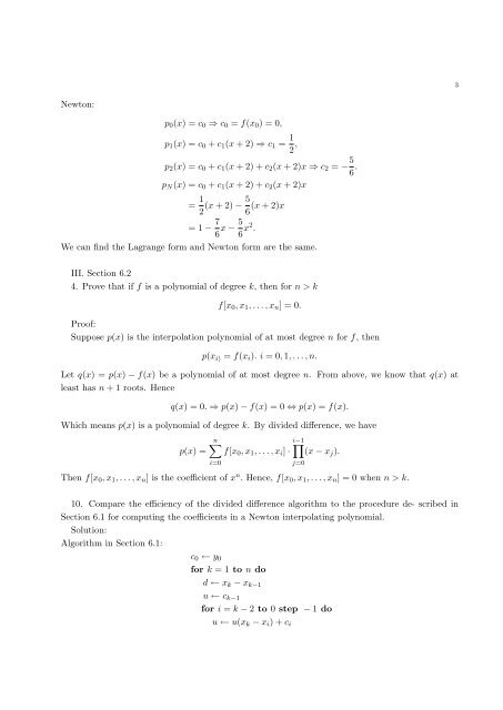
3Newton:p 0 (x) = c 0 ⇒ c 0 = f(x 0 ) = 0,p 1 (x) = c 0 + c 1 (x + 2) ⇒ c 1 = 1 2 ,p 2 (x) = c 0 + c 1 (x + 2) + c 2 (x + 2)x ⇒ c 2 = − 5 6 .p N (x) = c 0 + c 1 (x + 2) + c 2 (x + 2)x= 1 2 (x + 2) − 5 (x + 2)x6= 1 − 7 6 x − 5 6 x2 .We can find the Lagrange form and Newton form are the same.III. Section 6.24. Prove that if f is a polynomial of degree k, then for n > kf[x 0 , x 1 , . . . , x n ] = 0.Proof:Suppose p(x) is the interpolation polynomial of at most degree n for f, thenp(x i) = f(x i ). i = 0, 1, . . . , n.Let q(x) = p(x) − f(x) be a polynomial of at most degree n. From above, we know that q(x) atleast has n + 1 roots. Henceq(x) = 0. ⇒ p(x) − f(x) = 0 ⇔ p(x) = f(x).Which means p(x) is a polynomial of degree k. By divided difference, we havep(x) =n∑∏i−1f[x 0 , x 1 , . . . , x i ] · (x − x j ).i=0Then f[x 0 , x 1 , . . . , x n ] is the coefficient of x n . Hence, f[x 0 , x 1 , . . . , x n ] = 0 when n > k.j=010. Compare the efficiency of the divided difference algorithm to the procedure de- scribed inSection 6.1 for computing the coefficients in a Newton interpolating polynomial.Solution:Algorithm in Section 6.1:c 0 ← y 0for k = 1 to n dod ← x k − x k−1u ← c k−1for i = k − 2 to 0 step − 1 dou ← u(x k − x i ) + c i