Diurnal Cycling: Observations and Models of the Upper Ocean ...

JOURNAL OF GEOPHYSICAL RESEARCH, VOL. 91, NO. C7, PAGES 8411-8427, JULY 15, 1986Diurnal Cycling' Observations and Models of the Upper Ocean Response toDiurnal Heating, Cooling, and Wind MixingJAMES F'. PRICE AND ROBERT A. WELLERWoods Hole Oceanographic Institution, Woods Hole, MassachusettsROBERT PINKELScripps Institution of Oceanography, La Jolla, CaliforniaMeasurements made from R/P Flip using rapid profiling conductivity, temperature, and depth probesand vector-measuring current meters provide a new and detailed look at the diurnal cycle of the upperocean. A diurnal cycle occurs when solar heating warms and stabilizes the upper ocean. This limits thedownward penetration of turbulent wind mixing so that air-sea fluxes of heat and momentum are surfacetrapped during midday. The central problem is to learn how the trapping depth D T (mean depth value ofthe diurnal temperature and velocity response) is set by the competi_ng effects of wind mixing and surfaceheating. In this data set the diurnal range of surface temperature T s was observed to vary from 0.05

8412 PRICE ET AL.' DIURNAL CYCLINGTABLE 1. Flip 1980 Data BaseTypeSamplingSamplingRange Interval Precision CommentsprofilingCTD; T, C, PprofilingVMCM;V, T, PFixed levelVMCM' V, TWind speed UEppleypyranometer, I 0Air temperatures,cloud cover,pressure128.4 < t < 145.3 days* At = 2 min T _ 0.002øC2

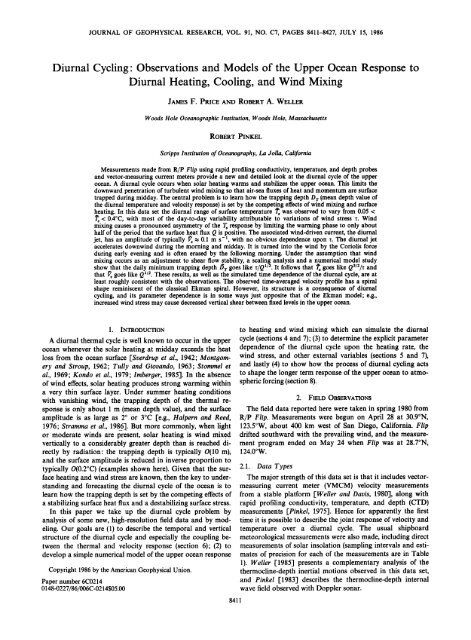
PRIC ET AL.: DIURNAL CYCLING 8413SURFACE HEAT FLUX........I' '"' I .... Io.o o.1 0.2WIND STRESS STRESS, N m -2T, z - 2, 10, 15, 20, 25 m' I '" I ' ' ! ' ' I I ' ' I ' I ' ' I' ' ' [ 'oHEAT CONTENTd • NET SURFACE' ' I' ' ' I ' " I ' ' I ' ' I ' ' I ' ' I ' ' I ' ' I '118 121 124 127 130 133 136 139 142 14,5TIME, daysFig. 1. Air-sea fluxes and overview of the temperature observations. (a) Heat fluxes. Insolation I (upper line) wasdirectly measured; heat loss L (lower line) was computed from air-sea measurements using standard methods. (b) Windstress computed from the observed wind using the bulk aerodynamic method. North is up. (c) VMCM-measured temperaturetime series at depths of 2, 10, 15, 20, and 25 m. (d) Observed heat content in the upper 40 m (solid line), and theintegrated air-sea heat flux (dashed line). Note that the rate of change of observed heat content differs greatly from theair-sea flux (presumably because of advection) except during a several-day period around 130.(temperature difference from 2 to 25 m, say) is generally dominatedby the diurnal cycle. The same is true for the verticalshear of the horizontal velocity. Hence one simple, and fairlyeffective way to separate out the signal: of the diurnal cycle isto compute the temperature and velocity vertical anomalies,T'(z, t)= T(z, t)- T( z. t)V'(z, t)= V(z, t)- v(z,, t)where the reference level z r should (1) be in a vertically homogeneouslayer to escape the effects of vertical advection andyet (2) be deep enough that the diurnal cycle amplitude at zr isnegligible. On days 128-131 a reference depth zr=40 mroughly satisfies conditions 1 and 2 above. For the record as awhole, there is no single suitable reference depth, and hencewhen dealing with the full record we are forced to work withstratification and shear (vertical differences over depths of lessthan the ideal zr) rather than temperature and velocity anoma-lies.3. DIAGNOSTIC LENGTH SCALESTo describe the structure of the observed temperature andvelocity profiles we will use the familiar jargon "mixed layer"to denote a quasi-homogeneousurface layer (temperatureuniform to within 0.02øC, velocity to within 0.01 m s-•) and"transition layer" to denote the stratified layer between themixed layer and undisturbed fluid beneath [e.g., Price, 1979].These are useful descriptive terms but are not alwaysuitablefor defining quantitatively a profile structure. As just one example,on days with strong winds the upper ocean may beonly very weakly stratified, and the mixed layer depth estilmated from field data can be quite sensitive to the somewhatarbitrary degree of homogeneity which defines the mixedlayer.At some risk of confusion we therefore suggest two newlength scales to measure the depth of surface trapping and thedepth of mixing. These length scales have the advantages ofbeing model independent and parameter free, and they can beobjectively estimated from field and model data. Both requirea profile of the temperature anomaly T'."Trapping depth" Dr is defined as the mean depth value ofthe temperature anomaly profile,Dr=T1 s ;• T' dz (1)

8414 PRICE ET AL.' DIURNAL CYCLINGß owhere in our case z, = 40 m, and z s = 2 m. In those profileswhere a mixed layer/transition layer structure is well defined,then Dr will lie near the middle of the transition layer. Thistrapping depth may be evaluated over each individual CTDobservedor model-computed profile."Penetration depth" De is defined as the length scale(O/Oz) -• of the one-dimensional heat equation, OT/Ot =(-1/poC ) (OF/Oz), where Po and c are the density and heatcapacity of sea water (both constant), and F is the heat fluxwhose surface value is Q. Penetration depth is estimated hereas the surface value of the length scale,i .... i .... i .... i .... 1 .... i .... i ....œ • t o• O '.LN•_LNOODe - pocOT•'/Ot (2)During the rising phase of the heating cycle when the heat fluxprofile is monotonically decreasing with depth (section 6), Dpis a direct measure of the depth of wind mixing.Both Dr and De may be written in terms of the heat content,H (kinematic units), of the temperature anomaly profile,H= T' dzßObviously,DT = H/T•'i .... i .... i .... i .... i .... I .... i ....œ • t ot,u 0 'IN31NOO 1¾3Hwhich makes clear that for a given H (which is imposed externally),the surface thermal response is inversely proportionalto the trapping depth. In the absence of advection, OH/Ot =Q/poC, and thenOHi .... i .... i .... i .... i .... i .... i ....œ • t o• O '.LN•I. NO0These suggest plotting H versus T•' hysteresis curves for thediurnal cycle (Figure 2) the way Gill and Turner [1976] did forthe seasonal cycle. On most days the hysteresis curves growalmost straight out from the origin until a few hours afternoon when they begin to turn counterclockwise (increasingheat content and decreasing surface temperature). The dailyminimum values,/•r and /•p, are thus nearly equal on mostdays (this need not be true in general).Note that between these four successive days there isroughly a factor of 4 difference in /5 r (or/•,) and a corre-sponding difference in the amplitude of Ts'. As we suggested inthe introduction, the key to understanding the diurnal cycle isto learn how these important day-to-day changes in the trappingdepth depend upon the day-to-day variability in theheating and wind stress.4. A MODEL OF THE UPPER OCEAN RESPONSE TOHEATING AND WINDMIXINGi .... i .... i .... I .... I .... i .... i ....œ z: t o•u O 'IN31NOO I•3H4.1. BudgetsThe diurnal cycle is modeled as a vertical mixing and radiationprocess driven solely by the local surface fluxes of heatand momentum [e.g., Niiler and Kraus, 1977]. We are therebyassuming that the diurnal cycle rides passively and noninteractivelyon top of the ambient oceanic variability. Underthis assumption the budget equations for the diurnal cycle arethe usual one-dimensional forms:OT -1 OF- (3)Ot poC Oz

PRICE ET AL.: DIURNAL CYCLING 8415- (4)c•tc•V1 c•G- fx (5)c•tPo c•zwhere the flux profiles are to be determined. The surfacevalues are presumed known: F(0)= Q, the air-sea heat flux,positive downward• E(0) = S(E- P), the freshwater flux timessurface salinity• and G(0), = z, the wind stress.The heat loss L is presumed to leave directly from the seasurface, while solar insolation is absorbed within the watercolumn with a double exponential depth dependence [Kraus,1972],I(Z) = •(0)[• 1 exp ( -- z/2,) + I: exp (-- z/22) ] (6)Subscripts 1 and 2 refer to the shortwave and long-wave componentsof insolation, and z is positive downward with z = 0being the sea surface. Paulson and Simpson [1977] provide theparameters of (6) for a wide range of oceanic water types. Inthe case of fairly clear, mid-ocean water (type 1A), which weassume holds for our measurement site in the open subtropicalPacific (30øN, 124øW),I1 = 0.6221 = 0.6 m12 = 1 - 0.62 2 2 = 20 mand thus about half of the solar insolation is absorbed withinthe uppermost meter of the water column. The remainingshortwave component of the insolation is absorbed with anextinction scale of 20 m.Absorption of radiation in the water column would by itselfyield a trapping depth of about 2 m. The observed trappingdepth is usually much greater, O(10 m), showing that the heatflux profile F(z) is usually determined more by wind mixingthan by radiation absorption alone.Density is calculated from a linear state equation,P = Po + o•(T - To) + fl(S- So) (7)where in this case Po- 1.025 x 103 kg m -3, T O - 17øC, y--0.23 kg m -3 øC-•, So = 36 parts per thousand (ppt), andfl = 0.76 kg m- 3 ppt- 14.2. MixingThe only artful part of such a model is its parameterizationof wind mixing. We have experimented with a fairly broadrange of mixing parameterizations (with help from P. Martinand P. Klein) and present the model which appeared to us tohave the most realistic parameter dependence and profilestructure (see Martin [1986] for extensive model comparisons).This model is essentially the dynamic instability model(DIM) mixed-layer model of Price et al. [1978] (see also Pollardet al. [1973] and Kronenburg [1985]) which is modifiedhere by including a mixing process in the stratified fluid belowthe mixed-layer.Vertical mixing occurs in this model in order to satisfy stabilitycriteria which require thatfor static stability,> o (8)c3z--gAphRb = po(AV) 2 > 0.65 (9)for mixed layer stability, andgc•p/•zR a = po(OV/Oz)2 > 0.25 (10)for shear flow stability. In the mixed-layer criterion (9), h is themixed-layer depth, and A( ) takes the difference between themixed layer and the level just beneath.In Appendix A we describe some model experiments thatshow the consequences of each of these three mixing processes.Briefly, the first mixing process simulates free convection,which occurs whenever there is heat loss from the sea surface(always in this data set). Free convection will cause mixingdown to the convection depth [Dalu and Purini, 1981], whichis quite shallow for the range of z and Q encountered in thisstudy, typically < 1 m at midday. The second mixing processsimulates mixed-layer entrainment by relaxation of an overallRichardson number, and the third mixing process simulatesthe effects of shear flow instability by relaxation of the gradientRichardson number. These latter two are by far the dominantvertical mixing processes for the z, Q range of this studyand are emphasized throughout. They may be regarded aswind-mixing processes in the sense that the velocity whichappears in the Richardson numbers is entirely wind driven,and both processes would be inactive if the wind vanished.Our motivation for using both a bulk and a gradient mixingprocess is discussed in the subsection below, in section 7, andin Appendix A.4.3. ImplementationThe model is set up on a high-resolution vertical grid, Az =« m, and run with time steps At = 900 s. At each time stepsolar insolation is absorbed according to (6), and the air-seaheat loss L and freshwater flux E - P are extracted from thetopmost grid level. The density profile is then calculated and ifnecessary adjusted to achieve static stability (equation(8)) bymixing from the surface downward to simulate free convection.The heat flux profile accompanying free convection is[see Deardorff et al., 1969],F(z) = F(O)(1 - z/h) (11)Wind stress is then absorbed within the mixed layer, themomentum balance is stepped forward in time, and the mixedlayerRichardson number Rb calculated. If Ro < 0.65, then themixed layer entrains successively deeper levels until (9) is satisfied.The heat flux profile that accompanies this wind-mixingprocess increases from the surface downward, has a maximumat the depth of the mixed layer,r(z) =z dh (12)aT aWand vanishes below. Similar terms appear in the salinity andmomentum budgets.To this point the model is exactly the DIM model of Priceet al. [1978], and like all conventional, bulk, mixed-layermodels [e.g., Denman, 1973] it assumes the existence of a sur-face mixed layer having a jump of density and velocity at itsbase. The field data shown here make clear that while a sur-face mixed layer is well included in an upper ocean model,there is certainly no sharp jump at its base. Instead, there is asmooth (at the several-meter scale), and sometimes quite thicktransition layer across which the mixed-layer temperature andvelocity match with the fluid below. This transition layer is a

8416 PRICE ET AL.' DIURNAL CYCLINGmajor feature of the observed profiles which has to be simulatedin the model before it is plausible to make a direct comparisonwith field data.Guided in part by the observations of Price [1979] (seereferences therein to atmospheric boundary layer studies) andby the presumption that sharp jumps are likely to be the sitesof shear flow instability, we have gone on to require that thegradient Richardsonumber R e be no less than a presumedcritical value, 0.25 [Turner, 1973; Thompson, 1980; Adamec etal., 1981]. R e is calculated by first differences over the stratifiedpart of the profile (not in the mixed layer). If the smallestR e in the profile is found to be less than the presumed criticalvalue of 0.25, then p, T, S, and V at the two grid levels thatproduce the smallest R e, say, j and j + 1, are partially mixedaccording to5. SCALE ANALYSISOne of the primary goals of this paper is to learn the explicitparameter dependence of the diurnal cycle. Given thatwe do not know an analytic solution of our model when heatingis applied, we attempt to deduce the parameter dependenceby a scaling and dimensional analysis.The analysis is simplified a good deal in the case when, ascommonly occurs, nighttime cooling and wind mixing producean early morning mixed layer which is somewhat deeper thanthe trapping depth of the coming day. The new diurnal cycle isthen written upon a "clean slate" [Stommel et al., 1969] whichhas no important memory of the previous day's stratificationor velocity. The external parameters which control the diurnalcycle are then those that describe the atmospheric forcing plusrotation.For simplicity, the surface heat flux is taken to be made upof a steady heat loss L and a sinusoidal insolation I (for nowassumed absorbed at the surface, i.e., 2• = 22 --0). The timescale of the heating, Po, is defined as half of the interval duringwhich Q > 0.5.1. Temperature and Velocity AnomaliesAssuming for the moment that the trapping depth Dr isknown, then from the heat equation (3) we can immediatelywrite down estimates of the temperature and density anomalies,and from (7),gT• QPa (13)DrPoC6p = o•gT (14)The coefficient required to make an equality in (13) is 0(1) butwill remain unknown until the scale analysis results are calibratedagainst the numerical model.Wind stress is assumed to be steady with amplitude • and,like the heat flux, to be trapped over a depth D r during a timeinterval proportional to Pa' The velocity anomaly is thengiven by the Fredholm solution [Phillips, 1977],•JV• • [2 -- 2 COS (ft)] 1/2Drfpowhere t - 0 is the start of heating. (It is easy to show that thevelocity anomaly is independent of the velocity left over fromthe preceding day [Price, 1979]). Further discussion of thescale analysis is limited to cases in which the heating timepj'=pj- 1 (p• p•+•)/2scale Pa is less than half the local inertial period. This effectivelylimits the scale analysis to low and middle latitudeswhere diurnal cycling is most important (and excludes thep•+ •' = p•+ • + 1 - (pj- p•+ •)/2nonetheless interesting case of high-latitude summer where thediurnal variability of heating gives way to a seasonal variawhere( )' is the value after mixing. Rg'= 0.3 is a specified bility). For the purpose of determining Dr the relevant velociconstantwhich is set just slightly larger than the critical valueto hasten convergence. (The choice Rg'= 0.3 versus, say, 0.25ty anomaly is that which occurs at about local noon, or t =Pa- It is convenient to define an acceleration time scale,is strictly for numerical convenience and has no appreciable which accounts for rotation,consequence in the solutions.) R• is then recalculated fromj 1 to j + 2, and the search and mixing procedure continues1until R• _> 0.25 throughout the stratified portion of the profile. e, = [2- 2 cosThe effect on the heat flux profile (equation(12)) is to smearout the otherwise sharp corner at z - h produced by mixed- and rewrite the velocity anomaly in the more compact formlayer entrainment.zP•6vDrPoFor a given Dr these estimates of the temperature and velocityanomalies follow directly from the budgets (equations(3)-(5)) and should obtain for any one-dimensional model.However, the dependence of Dr upon Q and r can vary greatlybetween different mixing parameterizations and hence so toowill the dependence of fit and 6 V.5.2. Trapping DepthThe notion behind our model is that wind mixing occursprimarily to relieve shear flow instability. The stability limit isgiven by a Richardson number criterion, and it might beguessed that a relation like (9) should obtain between thedensity and velocity anomalies and the length scale D r . Substitutionof (14) and (15) into (9) to solve for Dr in terms of theexternal variables r and Q, then gives the scale analysis resultthatDr • Q1/2 pal/2 (16)Elimination of Dr from (14) and (15) givesfit • Q3/2 pa3/2 (_0•/)1/2 (17)'r PT /90 c3/2P0Numerical experiments have verified that this is indeed theparameter dependence of our model. We expect it will hold forother models whose mixing parameterization depends upon amean flow Richardson number [e.g., Mellor and Durbin, 1975;

PRICE ET AL.: DIURNAL CYCLINO 8417AIR/SEA HEAT FLUXiIo-TEMP. PROFILESI I I0.0 0.3 0.6TEMPERATURE, C0 oTEMP. TIME SERIESz - 2,5,10 ... 40 rnCo-HEAT FLUX PROFILES-4 o 4 8HEAT FLUX, 102W m -2oxt ............... 10600;130 1200 1800 0000;131TIME;DAYFig. 3. Diurnal thermal cycle observed on day 130. (a) Air-sea heat flux. The heating period is shaded. (b) Temperatureprofiles measured by rapid profiling CTD. Time is to be read from the bottom of the profiles. Note that the upper 2 m wasnot sampled. (c) Temperature time series at depths of 2, 5, 10, ..-, 40 m. (d) Heat flux profiles calculated from the observedrate of change of temperature. Regions of warming are shaded.I0600Dickey and Simpson, 1983; Kondo et al., 1979], but probablynot those models built upon Monin-Obukhov scaling [e.g.,Gill and Turner, 1976; Garwood, 1979; Davis et al., 1981;Woods and Barkmann, 1986] or the classical diffusion model.(Under the assumption that no external time scale is relevantfor determining Dr, then dimensional analysis leads directly tothe Monln-Obukhov scaling Dr.,•r3/2/Q [Turner, 1973].From (13) and (15), 6T • Q2/z 3/• and 6V • Q/r •/•, which canbe quite different from (16)-(18). In particular, note that for agiven range of Q and z the Monin-Obukhov scaling will give alarger range of 6T than does (17).)In Appendix B the basic scaling results (equations(16)-(18))are developed further by accounting for (1) radiation absorptionat depth, (2) the constants needed to make equalities, and(3) the limit of vanishing r.6. DESCRIPTION OF THE DIURNAL CYCLETo illustrate the structure of the diurnal cycle, we havechosen two particularly clean and representative examples fora close look: the large-amplitude thermal cycle on day 130,which had light and somewhat variables winds, and the velocitycycle on day 131, which had fairly steady wind and also hadan appreciable thermal response. The full 25-day record isthen used to show the coupling between the thermal and velocitycycles and to begin to consider the day-to-day variabilityof the diurnal cycle.6.1. Thermal CycleIt is helpful to describe the thermal cycle partly in terms ofthe heat flux profile which is calculated by integrating the heatequation (3) upward from the reference depth [Deardorff et al.,1969],F(z)= po c ,• dzHeat flux profiles estimated from field data in this way areeasily contaminated by horizontal and vertical advection andcannot in all cases be interpreted as the consequence of alocal, vertical mixing or radiation process. However, the threemain stages of the thermal cycle described below from day 130occur repeatedly in the data and are thought to be genuinesignals of the diurnal cycle.Stage 1: Warming throughout. From sunrise until about

8418 PRICE ET AL.' DIURNAL CYCLINGnoon, the heat flux profile decreases monotonically from the to the Fredholm problem. In that case the wind stress is timesurface as warming occurs throughout the wate r column dependent; in this case the wind stress is steady (Or may be so(Figure 3). So long as the heat flux profile is monotonic, its imagined), but the stress penetration depth varies as part ofdecay scale can be measured by the penetration depth De the diurnal cycle.(section 3). Dp usually reaches a daily minimum value at An example of the diurnal velocity cycle is shown in Figurearound noon and on day 130 is fairly shallow, /•, _• 5 m. 4, where VMCM-measured velocity is shown as vectors atLevels above 5 m thus warm rapidly during midday, while at depths of 2, 5, 10, 15, ..., 40 m. Velocity is referenced to 40 mthe same time the heat flux is effectively cut off from deeper in an attempt to suppress the competing velocity signals fromlevels, > 15 m, which remain at a nearly constant temperature tides and ambient inertial and geo'strophic motions [Weller,throughout the morning (aside from some very weak warming 1985; Pinkel, 1983]. Some fine details of the velocity cycleby direct absorption of radiation evidenced by the smooth depend upon the reference depth, but the major features deincreasein stratification between 15 and 40 m).scribed here do not. A temperature profile from a simulta-Stage 2: Cooling and warming. Starting within a few hours neous CTD cast is plotted in the background, and the windafter noon, wind mixing begins to mix downward the heat stress is included as the topmost, dashed vector. Wind stressstored near the surface during midday and causes the heat flux changed direction slightly on day 131, but the magnitude wasprofile to develop a distinct knee, or middepth maximum(equation(12)). The knee in the heat flux profile correspondsclosely to the depth of the deepening surface mixed layer.Above the knee, or within the mixed layer, this wind mixingcauses rapid cooling during the early afternoon, even while thesurface heat flux remains fairly strong and positive. Windmixing thus causes a rather pronounced asymmetry in theresponse of surface temperature by limiting surface warmingto just a little more than a quarter of the day (observed alsoby Hoebet [1972] and Dickey and Simpson [1983]).Below the knee and over a depth that corresponds roughlyto the upper portion of the transition layer, vertical windmixing causes warming. Continued wind mixing pushes theknee downward through the water column during the lateafternoon and early evening. When the thermal response isstrongly surface trapped, as it was on this day, then at middepths,20-30 m, the warming phase of the diurnal cycle maybe very abrupt, lasting only the few hours required for thepassage of the heat flux knee and the associated transitionlayer. Cooling begins at a given level immediately after theknee passes, and along with the arrival of the mixed-layer.Stage 3: Cooling throughout. By about midnight, the downwardpropagation of the heat flux knee has reached to 30 mdepth. Thereafter, the heat flux profile is dominated by theheat loss to the atmosphere and again becomes monotonic,with cooling throughout the depth of the mixed layer (equation(11)). Heat loss continues until the following sunrise anderases the heat anomaly from day 130 before the warmingphase of the thermal cycle reaches below 35 m.6.2. Diurnal Jets and the Velocity CycleThe diurnal cycle has a profound effect upon the winddrivenvelocity. It produces a characteristic mode of variabilitythat we have dubbed the "diurnal jet" [Weller et al.,1983] and sets the vertical structure of the time-averaged,wind-driven transport (described in section 8).A diurnal velocity cycle comes about because heat and momentumare mixed in what appears to be a similar way, i.e.,the penetration depth for the momentum flux shoals duringmidday right along with the penetration depth for the heatflux discussed above. (This was first suggested for the ocean byMontgomery and Stroup [1962]; see also Kondo et al. [1979].For description of the nocturnal jet of the planetary boundarylayer, see Gill [1982], Thorpe and Guymet [1977], and alsoRubenstein [1981]). In addition, the wind-driven velocity issubject to the Coriolis force, which turns the velocity vectorcum sole (clockwise) during the day. The diurnal velocity cyclethus has some of the character of the inertial motion solutionroughly constant at about 0.08 N m-2.The velocity cycle is shown beginning at 0600 LT on day131 (topmost panel of Figure 4, time increases clockwisearound the figure), with a mixed layer of about 35 m thickness.By the next panel at 1000 LT, some heating has occurred anda warm surface layer has begun to form. Note that the momentumflux supplied by the wind stress appears to be surfacetrapped over a depth scale that is very similar to tha t fo r theheat flux. The result is a surface half-jet, or diurnal jet, in theupper ocean velocity profile (Strass[1983] and Woods andStrass 1'1986] have applied the term diurnal jet to the flow justbeneath the surface current we describe here). During th emorning the diurnal jet accelerates parallel to the wind stress.Its amplitude reaches a maximum in early afternoon of typicallyV s' -• 0.1 m s-•. The diurnal jet is constantly being rotatedcum sole by the Coriolis force, and by sunset it is almostperpendicular to the wind stress. Further rotation causes thediurnal jet to turn up into the wind, and by sunrise of the nextmorning the diurnal jet is nearly erased by the same windstress which created it during the previous day.6.3. Coupling of the Thermal and VelocityCyclesSome kind of diurnal thermal and velocity cycle occur oneach day of this experiment, though their amplitude and verti -cal structure can vary a good deal from day to day. To beginto see this we have plotted the full VMCM record in the formof the temperature difference and vector velocity differencebetween 2 m and 25 m (Figure 5) along with the model solution.Dashed lines are superposed at 1400 LT on each day. Aswas discussed in section 2, differencing two near-surface levelswill serve to suppress somewhat the effects of horizontal advection,but even so there remain other competing phenomenawhich partially obscure the diurnal cycle. There are at leasttwo instances of temperature inversions which appear to begenuine, days 135-136 and 140-141 (these suggesthat salinitymust have been important at least intermittently but was notmeasured by VMCMs), and also higher-frequency inversionswhich may be measurement noise (VMCM least count, Table1). Further, 25 m is too shallow to be an appropriate referencelevel for calculating anomalies, and hence these differences willbe referred to as stratification and shear (but not normalizedby the depth interval). Even with these drawbacks, the fullrecord serves to make two important points.First, on almost every day both the stratification and sheargo through a distinct maximum at about 1400 LT, the timewhen the surface amplitude of the diurnal cycle is usually amaximum, and then go through a minimum in the early

PRICE ET AL.' DIURNAL CYCLING 84 !9E.__....... '-.. 0600, 131-i 0200,lOO0,•o '" """":,:--' 2200, 131i • '"--.i', ..... 1•oo, 1•1• ..... 00, 131• • 0.Fig: 4, Diu•"al •½løcity cycl• observed o• d•), I3!. The ¾]VIC]VI-•½asu•½d velocity is •½f½•½•ccd to 40 •. The topmostdashed Vector is the wind stress, and the temperature profile is plotted in the background. Local time and day are markedon the lOWe right in each panel.

8420 PRICE ET AL.' DIURNAL CYCLINGßß ß oA ø ß ß ß ß ß ß ß ß ß ß' ' I ' ' I I ' I ' I I ' ' I ' ' [ ' ' I ' ' I ' ' I118 121 124 127 130 133 136 139 142 145TEMP DIFFERENCE, 2 - 25 m, , I , , I , , I , , I , , I , , I , , I , , I , , I ,oOBSE'RVEDi :: i :: i :: :: :: :: :: :: :: :: :: :: :: ::' '' i ' ' I ' ' I ' ' I ' ' I ' ' i ' ' i ' ' I ' ' i '118 121 124 127 130 133 136 139 kt2 145VEL DIFFERENCE, 2 - 25 mo [ ' ' , , i , • , , , i t ....I I I I I I I I I118 121 124 127 130 155 156 159 142TIME, do¾sFig. 5. The full record of temperature and velocity differences. (a) Wind stress amplitude and daily maximum surfaceheat flux (dots).(b) Temperature difference from 2 to 25 m observed by VMCMs (top) and modeled (bottom).(c) Velocitydifference as above. The dotted lines are at 1400 LT each day.morning when the temperature and velocity mixed layersreach below 25 m. This daily modulation of the upper oceanshear shows the crucial role that heating and stratificationmust play in setting the vertical structure of the time-averagedwind-driven velocity (more on this in section 8).Second, there is very large day-to-day variability in the amplitudeof the stratification and shear, and there is some evidencethat they covary. During a period of very light windsand strong heating, days 125-127, the midday maxima wereespecially large in both stratification and shear. During thetwo days with the heaviest winds and lightest heating, days121 and 144, the maxima in stratification and shear were quiteweak. Thus the vertical shear of the wind-driven velocity displaysa dependence upon wind stress amplitude that can bejust opposite that of a classical wall layer or Ekman layer.How this happens is taken up in the next section, where weexamine the parameter dependence of the diurnal cycle.7. PARAMETER DEPENDENCE AND MODEL RESULTS7.1. Thermal CycleMost of the day-to-day variability in the diurnal thermalcycle found in this data set is due to the variations of windstress magnitude. This may be seen in a qualitative way in theVMCM record of Figure lc; the days with the smallest T•response (days 121-122 [roughly 0.05øC], 128-129, and 135-136) are the days with the largest wind stress, while the dayswith the largest response (days 123-126 [roughly 0.4øC] and135-136) are the days with the smallest wind stress. The importantrole of wind mixing under these moderate, fair weatherconditions has been observed before [Sverdrup et al.,1942; Hoeber, 1972; Pollard, 1977; Kondo et al., 1979; Simpsonand Dickey, 1981].To assess the quantitative effect of wind stress and heatingvariations, we limit our view to days 128-131, which the heatbudget showed were relatively untroubled by horizontal advection(Figure lt0. The CTD data and the model solutionfrom these four days are shown as profiles in Figures 6c and6d and as time series of temperature at fixed depths in Figures7c and 7d. There are advective effects evident even here: notethat the observed 30-m temperature (Figure 7c) is more variablethan the modeled 30-m temperature and shows a coolingtrend not found in the model. The diurnal cycle signal is easilyseen, however, and the high-resolution CTD data make it possibleto calculate the trapping depth (Figure 6e) and the penetrationdepth (Figure 7e) from (1) and (2). These 4 days span afairly wide range of maximum heating and wind stress (Table2), and the diurnal cycle varies considerably over this period(recall also Figure 2).

PRICE ET AL.' DIURNAL CYCLING 8421?ESURFACE HEAT FLUXXoI .... I .... I --2WIND STRESS o.o o.1 o.2 N mIll l 1OBSERVEDTEMPERATURE PROFILES o o o.3 o 6 CMODELLEDEd ...... i , , ' ' i ' ' ! , , i , , f , , i ' ' i , ,TRAPPING DEPTH•,• ' ' i ' ' • ' ' i ' ' i , , i ' ' i ' ' i ' , I ' , i ' ' i , , i ' ' i , , i , ' i , , i ' ' i128.5 129 129..5 130 130.5 131 131..5 132TIME, do¾sFig. 6. CTD and model data from the period from day 128 to day 131. (a) Air-sea heat flux. (b) Wind stress. (c)CTD-measured temperature profiles. Note that the upper 2 m was not sampled. (d) Model-computed profiles. (e) Trappingdepth calculated from individual CTD profiles (one dot per profile), and from the model data (solid curves).We can see the effect of r variation by comparing days 128and 130, which have roughly equal Q, while r on day 128 wasabout a factor of 4 larger than r on day 130. The result wasthat/•r on day 128 was about a factor of 4 larger than that onday 130, or roughly proportional to the ratio of wind stresses;metry of the surface thermal response noted in section 6.1.Most importantly, the model simulates well the day-to-dayvariability of the diurnal cycle, which also suggests that themodel has a parameter dependence consistent with these data.These results are encouraging, but comparison with a moreextensive and less complicated (by nonlocal phenomenon)data set would be required to reach any stronger conclusion.(See Stramma et al. [1986] for a comparison against a somewhatlarger data set spanning a much wider range of conditions.)The simple scale estimates (Appendix B) listed in Table 2•s on day 128 was about a factor of 4 smaller than that on day130, or inversely proportional to the ratio of wind stresses.The scaling analysis (equations(16) and (17)) is consistent withthis observed • dependence.We can see the effect of Q variation by comparing days 129and 131, which have roughly equal r, while Q on day 131 wasapproximately twice that on day 129 (owing mainly to increasedcloud cover on 129). Doubled Q causes both a smalleralso make fairly good predictors of •s and/•r. For some purposes,say, estimating the day-to-day variation of the ratio of/5 r (a little less than a factor of 2) and a larger •s(a little more photic zone depth to the wind-mixing depth [Marta and Heinthana factor of 2). The scaling analysis (equations(16) and(17)) is also consistent with this Q dependence.emann, 1982] or forecasting the diurnal cycle [Clancy and Pollack,1983], these scale estimates may be as useful as the fullThe numerical model gives a fairly faithful simulation of theoverall structure and amplitude of the diurnal cycle on these 4numericalevaluate.model solution and of course are much easier todays. The model-computed amplitudes and the trapping depth(and to a lesser degree, the penetration depth) show no obviousbias, suggesting that the model does roughly enough windmixing. The model solution also reproduces well the asym-7.2. Diurnal ,let AmplitudeA diurnal jet of the sort described in section 6.2 will occurin any upper ocean model which assumes that heat and mo-

8422 PRICE ET AL.' DIURNAL CYCLING?ESURFACE HEAT FLUXOBSERVEDT, z - 2, 5, 10, 1.5, 20, 25, 30 m' ' I ' ' I ' ' I ' ' I ' ' i ' ' I ' ' I ' ' i ' ' i ' ' I ' ' I ' ' I ' ' I ' ' 1 ' ' I ' ' IMODELLED' ' I ' ' i 'PENETRATION DEPTH.... I ' ' I ' ' I ' ' i ' ' I ' ' I ' ' I .... I ' ' I ' ' I ' ' i ' I i128.5 129 129.5 130 130.5 131 131.5 132TIME, do¾sFig. 7. CTD and model data from the period from day 128 to day 131. (a) Air-sea heat flux. (b) Wind stress. (c)CTD-measured temperature time series at depths of 2, 5, 10, 25, and 30 m. (d) Model-computed temperature time series. (e)Penetration depth calculated from the CTD data (heavy dots) and from the model data (solid curves).mentum are mixed in a more or less similar way [Kondo et al.,1979; Woods and Strass, 1986]. The amplitude and parametricdependence of the diurnal jet will, however, vary from modelto model depending upon the wind-mixing mechanism andparameterization.An at first curious result of the scaling analysis of our model(section 5) was that the diurnal jet amplitude was found toscale asExplicit dependence upon ß vanishes because while 6V goeslike r/D r , the trapping depth D r is itself proportional to•/Q•/2. Variations of wind stress alone are thus expected tocause variations in the thickness of the diurnal jet rather thanin the amplitude.Some evidence of this may be seen in Figure 8, which showsthe magnitude of the velocity referenced to 40 m for days128-131. The daily peaks of this velocity make rough estimatesof •s' uncertain to about 0.02 m s-• because of uncer-tainty in the reference level. Though ß varies by about a factorof 4 from day 128 to day 130, the diurnal jet amplitude variesfrom only about 0.12 m s -• to 0.10 m s -•. Note that dayswith the larger •, 129 and especially 128, have a comparativelythick diurnal jet. This is consistent with the day-to-day variationof/5 r already noted for the thermal response and withthe r variation expected from the scaling analysis. We mighthave expected to see a weak dependence of • upon Q andTABLE 2. Diurnal Cycle Parameters and Scales for Days 128-131Day 128 Day 129 Day 130 Day 131Parametersr, N m -2 0.13 0.07 0.03 0.07I, W m-2 829 552 833 978L, W m -2 -195 -144 -105 -126Q, W m-2 634 408 728 852Pa, day 0.20 0.19 0.20 0.22P,, day 0.18 0.17 0.19 0.20Scale Estimates*•, øC 0.09 0.07 0.36 0.25D r, m 19 15 6 10•, m s-t 0.10 0.07 0.10 0.11Observedt•', øC 0.08 _+ 0.02 0.10 _+ 0.02 0.34 _+ 0.04 0.22 _+ 0.02Dr, m 21 +2 16_+2 5_+ 1 9_+1•', m s-t 0.12 _+ 0.02 0.11 _+ 0.02 0.10 _+ 0.02 0.10 _+ 0.02*Made from the formulae in Appendix B.•'Eyeball estimates from Figures 7, 6, and 8.

PRICE ET AL.' DIURNAL CYCLING 8423Fig. 8. Magnitude of the vector velocity difference from 40 m as afunction of depth and time for the period from day 128 to day 131.The daily maximum values are reasonably good estimates of the diurnaljet amplitude.thus a slightly larger •s on 130 than on 128. This weak Qdependence is not apparent in Figure 8.7.3. Profile StructureDuring many afternoons the temperature and velocity profilesdevelop a fairly clear-cut two-layer structure with a surfacemixed layer above a stratified and sheared transition layer(Figures 4 and 6). Temperature mixed layers are a very familiarfeature in ocean data and are often built into upper oceanmodels (including ours; see also Niiler and Kraus [1977] andGatwood [1979]). It is particularly striking that on day 128 asurface mixed layer of at least 10-m thickness persisted rightthrough the day despite strong heating (best seen in the timeseries of Figure 7c). Models which assume that fluxes are proportionalto the local vertical gradient times a diffusivity [e.g.,Kondo et al. [1979] or the "gradient mixing only" solution ofAppendix A) tend to develop substantial near-surface gradientsunder these conditions. In this respect they may be lessrealistic than simpler mixed-layer models which take a surfacemixed-layer for granted.These data show that a velocity surface mixed layer is alsopresent and is at least roughly coincident with the temperaturemixed layer. For example, a velocity mixed layer of about30-m thickness exists at 0600 LT on day 131 (Figure 4), coincidentwith the temperature mixed layer, even though themixed layer was absorbing a stress of about 0.08 N m-2. Thevelocity mixed layer seems to disappear during midday whennear-surface stratification develops as part of the diurnal thermalcycle (that it disappears depends on the vertical samplinginterval) and then reappears along with the temperature mixedlayer at 1800 LT on day 131. At that time the surface mixedlayer was absorbing both a surface stress of about 0.08 N m-2as well as an entrainment stress, and again there is little sustainedvertical shear of velocity within the temperature mixedlayer (no more than about 10-3 s-•). Some process which wecan not directly identify in these data, perhaps large-scaleeddies like Langmuir circulations [Weller et al., 1986], mustbe acting to overturn the mixed layer within tens of minutes.On days with stronger winds, the velocity mixed layer mayremain deep right through the day, just as we noted above forthe temperature mixed layer. Thus stronger winds may produce(contrary to intuition and to classical theories whichignore stratification altogether) reduced shear between fixedlevels in the upper ocean (section 6.3).Our model produces a realistic profile structure because webuilt in a surface mixed layer at the outset (thickness is givenby (9)) and allowed for a smooth transition layer by admittingmixing below the mixed layer (according to (10)). Duringmidday, when the transition layer is thickest, active verticalmixing occurs through only about the upper half of themodel's transition layer, while the lower half is quiescent. Thedensity difference Ap felt by the bulk Richardson number condition(equation(9)) will then be less than the surface densityanomaly tSp, and the gradient Richardson number averagedacross the full transition layer will be somewhat greater thanthe critical value at which active mixing begins. Sometimeafter sunset, once surface heat loss has reduced the heat anomalyof the diurnal layer, vertical mixing will usually be activethrough the full depth of the transition layer, and then thecriticality condition on the Richardson numbers may bechecked against the observations using the easily observedsurface anomalies. For example, at 1800 LT on day 131(Figure 4) there is a velocity change of about 0.1 m s-• (thefull amplitude of the diurnal jet) over a 10-m-thick transitionlayer (15 to 25 m) across which the temperature change isroughly 0.1øC (density change of about 0.023 kg m-3). These'T O-7'b-7 ..... 0 1EAST, 10-2m s -•Fig. 9. Time-averaged velocity for the period from day 120 to day 145. (a) VMCM-measured velocity, referenced to 70m. The topmost vector is the time-averaged wind stress. (b) Hodograph plots of the observed (solid curve) and modelcomputed(dashed curve) time-averaged velocity. Depth is shown by symbols every 4 m, starting from 2 m. In both casesthe zero or reference velocity has been placed at 70 m.

8424 PRICE ET AL.' DIURNAL CYCLINGgive Rg • ¬ (averaged across the transition layer) and Rb--«(mixed-layer depth measured to the middle of the transitionlayer is 20 m), or grossly consistent with the values assumed inthe model, This shows too that what would seem to be a verysmall temperature difference, 0.1 øC, can sustain the full diurnaljet, consistent with the Rg condition. Thus even very weakstratification may be crucially important in determining thevertical structure of the wind-driven velocity.and zr is the reference depth. Transports estimated from thedata, the Ekman transport, and the model transport areobserved, z, = 50 mobserved, z, = 70 mmodeledEkmanM xMy-0.9 0.4- 1.6 0.21.0 0.1- 1.0 0.18.1. Velocity Spiral8. THE TIME-AVERAGED RESPONSEWe have seen in the two previous sections that in fair weather conditions the instantaneous, wind-driven, upper oceanVelOcity is usually dominated by the diurnal jet. Not surprisinglythen, the time-averaged, wind-driven velocity (Figure9a) has a spiral structure which can best be understood as aproduct of diurnal cycling (imagine taking the time averageover the diurnal velocity cycle of Figure 4). The time-averagedvelocity is surface intensified, as is the diurnal jet, and themodel is, trivially, the same as the Ekman transport. On theother hand, the transport estimated from the observations dif-•near-surface velocity points well to the right (cum sole) of thefers from Ekman transport by up to 50% (using z•- 70 m).time-averaged wind stress (•60ø). The time-averaged velocityWe suspect that the discrepancy between the observed transdecreasesand turns to the right with increasing depth becauseport and Ekman transport arises mainly from a thermal windthe diurnal jet decays and turns to the right as it penetratescontribution to the time-averaged shear, but we cannot verifydeeper into the water column during early evening.this with the available data.At first glance this observed spiral resembles an Ekmanspiral, but there are important differences in the structure and 8.3. Fluxesrather profound differences in the dynamics. Compared withWhile we are unable to say anything very definite about thean Ekman spiral, this spiral is rather fiat in that the velocitymagnitude of the observed transport, we have learned that inamplitude decays with depth considerably faster than the vefairweather conditions the process of diurnal cycling deterlocityvector rotates to the right with depth (noted too bymines how deeply the wind-driven transport penetrates theWeller [1981]). But more important, the vertical shear of theupper ocean and thus determines which water makes up thewind-driven velocity is closely tied to stratification, which isEkman transport. Figure 4 shows that the fastest flowing partaltogether ignored in the classical Ekman theory. In the abofthe diurnal jet (during early afternoon) is also the warmestsence of heating and the resulting stable stratification, for exwaterin the diurnal thermal cycle. The result is a persistentample in the nighttime mixed layer, there is only very weakvelocity-temperature correlation and a resulting "eddy" heatvertical shear and certainly no spiral of the sort found onflux over and above the heat flux due to the time-averageaverage over one or several diurnal cycles. On the other hand,transport. In this case the additional heat flux is roughlyif the heating had been stronger or the wind stress weaker,then it can be anticipated that the velocity spiral would have-1poc (U'T', V'T') dz ...(0, -3) x 106 W mbeen more strongly surface trapped (recall the differences be-tween days 128 and 130 seen in Figure 8).A velocity spiral of this kind should be present in the timeaverage whenever the upper ocean is undergoing diurnal cycling.We suggesthat it be termed the "diurnal cycle spiral" todistinguish it from the classical Ekman spiral and to emphasizethe vital role of heating and stratification.8.2. TransportIt is well known that the wind-driven mass transport isindependent of the form of vertical mixing or the structure ofthe velocity spiral. If no forces other than wind stress androtation act upon the water column, then aside from samplingerrors the observed transport,•z 0 --_(M,•, My)fß = (U, V) dzshould equal the Ekman transport,where the time-averaged wind stress in this case is1(•,,, •y)= (-0.008, -0.087) N m -2ßwhere M,• and My are in square meters per second. Whenestimating transport from the observations, we have taken thereference depth zr to be 50 m, which has below the mixedlayerdepth at most times during the experiment, and alternatively70 m, which was deeper than the mixed layer at anytime. It could be argued that either of these reference depths isappropriate, and hence the difference in transport is a measureof the uncertainty of the estimate.Transport computed from the time-averaged velocity of the•5 ø o(which is small by most standards) and is nearly parallel to thetime-averaged wind stress. Advection by the diurnal jet can beexpected to produce an enhanced horizontal transport of anyproperty which has a diurnal depth dependence, e.g., perhapssome phytoplankton species. (A similar kind of temperaturevelocitycorrelation and eddy heat flux might be expected overan annual cycle.)9. CONCLUSIONS AND REMARKS1. The diurnal cycle is an important mode of fair weathervariability which arises when solar heating stabilizes the surfacelayer and causes the surface fluxes of heat and momentumto be surface trapped during midday. Heat and momentumfluxes appear to be mixed in a similar way, so that the thermaland velocity cycles are closely coupled. Temperature and velocityprofiles observed during the afternoon often show atwo-layer structure, with coinciden temperature and velocitysurface mixed layers overlying a thick, stratified and shearedtransition layer.2. We have modeled the diurnal cycle with a very simplemixed-layer model which allows for mixing in the stratifiedfluid below the mixed layer. This model gives quite realistic

PRICE ET AL.' DIURNAL CYCLING 8425I ' ' I ' ' I0.0 0.3 0.6TEMPERATURE, CNO WIND MIXINGGRAD ENT MIXING ONLYE•E o -BULK MIXING ONLYFLIL L MODEL0600 1200 1800 2400 0600HOURO6.o .... 1200 . ..... 180 .... 2400 , ..... 0600 ,HOURFig. 10. Mixing experiments run using the numerical model with one or both wind-mixing processes shut off forcomparison to the full model (lower right).profile structures and has some successimulating the ampli- parameters is very shallow, roughly « m during midday. Thustude and day-to-day variability of the diurnal cycle.without wind mixing, the thermal response is very strongly3. Our model presumes that wind-mixing is a consequence surface trapped and its surface amplitude is extremely largeof shear flow instability. In that event, the trapping depth of (Figure 10);/5 r -- 1.5 m, and •s = 1.6øC. This very unrealisticthe thermal and velocity response is proportional to •/Q1/2, simulation demonstrates the crucial role that wind mixingperhaps the most important result of this paper. It follows that must have played on this day in distributing heat through athe thermal response is proportional to Q3/2/• and that the much thicker surface layer than can be reached by convectivediurnal jet amplitude is proportional to Ql/2. These are consis- processes and direct radiation absorption alone. (When thetent with our observations but require testing against a larger wind nearly dies [e.g., Halpern and Reed, 1976; Stramma et al.,and less complicate data set than was available here. 1986], then this radiation/convection envisioned by Kraus and4. The time-averaged profile of wind-driven velocity which Rooth [1961] and Dalu and ?urini[1981] will obtain.]makes up the Ekman transport has a flat, spiral shape as aA2. Mixed-Layer Entrainment Onlydirect consequence of diurnal cycling. In this regard at least,the process of diurnal cycle plays an important role in shaping With Rg set to zero the model reduces exactly to the conthelong-term response of the upper ocean to atmosphericventional, bulk mixed-layer model DIM of Price et al., [1978]forcing.(see also Pollard et al., [1973]). This model gives a reasonableaccount of wind mixing in an overall sense and thus gives aAPPENDIX h' MIXINGEXPERIMENTSTo see the consequences of the three mixing processes identifiedin our model (section 4), i.e., (1) free convection, (2)mixed-layer entrainment, and (3) shear flow instability, wehave carried out some very simple numerical experiments inwhich we arbitrarily shut off one or both of the wind-mixingprocesses, (process 2 and/or 3). These experiments are runusing idealized forcing (steady wind stress, steady heat loss,and sinusoidal insolation) whose values are approximatelythose of day 131' I = 980 W m-2, L = - 125 W m -2, PQ = 5hours, and z = 0.07 N m -2. The observed diurnal thermalcycle on day 131 had a response (Table 2) of Dr = 9 m andT• = 0.22øC, which can serve as a guide to reasonable values.A1. Free Convection OnlyWind mixing may be shut off in the model by setting bothRb and Rg to zero. Vertical mixing by free convection will thenoccur only down to the convection depth, which for thesegood account of the surface response'/ST = 10 m, and •s =0.23øC. However, the profile shape given by this model isgrossly unrealistic in a way that is characteristic of all mixedlayermodels [e.g., Denman, 1973]' in place of the smooth,thick transition layer found at the base of the oceanic mixedlayer, there is instead an abrupt jump whose thickness is justthe grid interval. For problems in which the profile shape isimportant, i.e., acoustic propagation or heat budgeting, then aconventional, bulk mixed-layer model may be too severe anidealization.A3. Gradient Mixing OnlyWith Rb set to zero the model mixes locally the density andvelocity profiles just enough to satisfy the shear flow stabilitycriterion that the gradient Richardson number should be nolarger than ¬. This too gives a fairly reasonable account ofvertical mixing in an overall sense' /5 T = 8 m, and • =0.27øC. But now the profile structure is unrealistic in a way

8426 PRICE ET AL.' DIURNAL CYCLINGthat just complements the bulk mixed-layer model notedabove. This model can not produce a surface mixed layer bywind mixing alone; a surface mixed layer develops only aftersunset by the free convection process. The field data on theother hand, show that a well-defined temperature and velocitymixed layer can persisthrough the day provided that thewind stress does not vanish.In the limit of vanishing wind stress, the wind-mixing scaleestimates must fail; e.g., •s becomes infinite. The scaling mustA4. Full Modelchange over to a different form, governed by free convectionWith both wind-mixing processes acting at once, the model- and 'radiation absorption (i.e., the no-wind-mixing case of Apsimulatedprofile develops a two-layer structure which is qual- pendix A). The mixing depth is then the convection depth Citatively like that observed in the ocean. There is a surface [Dalu and Purini, 1981] at which the heating rate by insomixedlayer which is as thin as 4 m near noon, bounded below lation is equal to the heat absorbed above z = C within aby a smooth transition layer whose thickness is roughly 20 m surface mixed layer, i.e.,near noon. In the full model the task of satisfying the stabilitycriterion by means of wind mixing is shared between the twoRichardson number criteria, and the net result is about as [I(0)- l(C) C + L] 0Imuch wind mixing as occurs by the mixed-layer entrainmentGiven the insolation absorption profile (equation (6)), the dailyprocess alone' •r = 9 m, and •s = 0-21øC- To the extent that minimum convection depth • may be easily calculated fromthe profile structure matters (rather than just the surface re-(23) given L and the daily maximum I.sponse), the full model is clearly preferable to the conventional As before, we presume that (13) holds, and calibrationmixed-layer model or to the gradient-mixing model.againsthe corresponding numerical model solution showsthat the leading constant is 1.0. The effect of penetrating solarAPPENDIX B' FURTHER DEVELOPMENT OF THE insolation has already been accounted for in C, and no JSCALING ANALYSISfunction is needed. The trapping depth may be evaluated fromBy a fairly straightforward extension of the scaling analysis its definition (equation (1)), together with the known • and •swe can derive a complete, accurate, closed form "solution" for and assuming that T(z)= Pe(Ol/Oz)/po,•, at depths below z =/•s,•s, and 17 s. To do this, we have to account for the effects of(7. The daily minimum trapping depth Dr isradiation absorption at depth, find the constants needed tomake equalities, and lastly, consider how the physics mustD~r - C~+I(C)•s pocchange in the limit of vanishing z.B1. Radiation AbsorptionWhen the absorption of insolation is considered, then adimensional analysis gives that each of (16)-(18) must bemultiplied by some function J(Dr/,•2), where recall it2 is theshortwave extinction scale of (6). Inspection of (6) togetherwith trial and error have given a form of J.[ l-Lexp(-Or/J,2)] (19)J(DT/J,2) = 1 -- 12 IB2. Calibration Against the Numerical ModelTo find which form of the scaling holds for a given r and Q,we calculate both forms and then compare the two estimatesThe scaling analysis has been calibrated against solutions ofof/•r. The deeper value invariably conforms to the numericalthe numerical model in order to find the leading constants for model result. For example, if the free convection/•r is found(16)-(18)[which were expected to be O(1)] and to find the best to be less than the wind-mixing 15r, then wind mixing wouldfit exponent on J. The scale estimates were first calibrated in have dominated for those conditions, and the wind-mixingthe limit of vanishing it: (J = 1) to find the leading constants,scaling obtains. This gives the result of selecting always theand then this preliminary estimate of Dr was used in J to then smaller •s and •.find the power law dependence upon J for finite it:. This last These scale estimates make an easily evaluated proxy forstep of the calibration is approximate and introduces a small the full numerical model and also serve to show the expliciterror, generally no more than about 10%. The end result is dependence upon all of the important known external varithewind-mixing regime form of the scaling analysis which ables. We caution though that they have been derived underholds throughouthe range of z and Q encountered in this somewhat restrictive conditions, and may not be accurate ifstudy. The daily minimum trapping depth/•r isconditions differ too strongly from those assumed (e.g., steadywind).j- 3/2 (20)Dr = 0.45 QY/2 pQ•/2the range of surface temperature • is•sQ3/2= 1.5 pQ3/2z P, po c3/2(__O•g),/•2 j3/2 (21)and the diurnal jet amplitude fs isB3. Free Convection Limitthe range of surface temperature Ts isand the diurnal jet amplitude •s isB4. Choosing the Scaling(22)I (23)Pe (24)•s = I(0)- 1((7) + L Pe (25)Cpoc-r P, (26)rS-Cp øAcknowledgments. We are grateful to the Office of Naval Researchfor their support of this program through contract N00014-76-C-0197, NR 083-400 with the Woods Hole Oceanographic Institution,(R. A. W. and J. F. P.) and contract N00014-75-C-0152 with ScrippsInstitution of Oceanography (R. A. W.). Development and operationof the CTD system was funded through the Office of Naval Research

code 200 and code 220 and Naval Ocean Research and DevelopmentActivity code 540 (R. P.). We thank R. Michael Clancy, Pijush K.PRICET AL.: DIURNAL CYCLING 8427Kundu, Paul J. Martin, and the referees for their helpful comments onthis paper. Woods Hole Oceanographic Institution contribution 5427.Pinkel, R., Doppler ,sonar observations of internal waves: Wavefieldstructure, J. Phys. Oceanogr., 13, 804-815, 1983.REFERENCEsPollard, R. T., Observations and models of the structure of the upperAdamec, D., R. L. Elsberry, R. W. Garwood, and R. L. Haney, An ocean, in Modeling and Prediction of the Upper Layers of the Ocean,embedded mixed-layer-ocean circulation model, Dyn. Atmos. Edited by E. B. Kraus, pp. 102-117, Pergamon, New York, 1977.Oceans, 6(2), 69-96, 1981.Pollard, R. T., P. B. Rhines, and R. O. R. Y. Thompson The deep-Bruce, J. G., and E. Firing, Temperature measurements in the upper ening of the wind-mixed layer, Geophys. Fluid Dyn., 4, 381-404,10 m with modified expendable bathythermograph probes, Journal 1973.of J. Geophys. Res., 79, 4110--4111, 1974.Price, J. F., Observations of a rain-formed mixed layer, J. Phys.Clancy, R. M., and K. O. Pollack, A real-time synoptic ocean thermal Oceanogr., 9, 643-649, 1979.analysis/forecast system, Prog. Oceanogr. 12, 383-424, 1983.Price, J. F., C. N. K. Mooers, and J. C. Van Leer, Observation andDalu, G. A., and R. Purini, The diurnal thermocline due to buoyant simulation of storm-induced mixed-layer deepening, J. Phys.convection, Q. J. R. Meteorol. $oc., 108, 929-935, 1981.Oceanogr., 8, 582-599, 1978.Davis, R. E., R. DeSzoeke, D. Halpern, and P. Niiler, Variability in Rubenstein, D. M., The daytime evolution of the East African jet, J.the upper ocean during MILE, I, The heat and momentum bal- Atmos. Sci., 38, 114-128, 1981.ances, Deep Sea Res., 28, 1427-1451, 1981.Simpson, J. J., and T. D. Dickey, Alternative parameterizations ofDeardorff, J. W., A. E. Willis, and D. K. Lilly, Laboratory investi- downward irradiance and their dynamical significance, J. Phys.gation of nonsteady penetrative convection, J. Fluid Mech., 35, Oceanogr., 11, 876-882, 1981.7-31, 1969.Soloviev, A. V., and N. V. Vershinsky, The vertical structure of theDenman, K. L., A time-dependent model of the upper ocean, J. Phys. thin surface layer of the ocean under conditions of low wind speed,Oceanogr., 3, 173-184, 1973.Deep Sea Res., 29, 1437-1449, 1982.Dickey, T. D., and J. J. Simpson, The influence of optical water type Stommel, H., K. Saunders, W. Simmons, and J. Cooper, Observationson the diurnal response of the upper ocean, Tellus, $er. B, 35, of the diurnal thermocline, Deep Sea Res., 16, 269-284, 1969.142-154, 1983.Stramma, L., P. Cornilion, R. A. Weller, J. F. Price, and M. G.Garwood, R. W., Jr., Air-sea interaction and dynamics of the surface Briscoe, Large diurnal sea surface temperature variability: Satellitemixed layer, Rev. Geophys., 17, 1507-1524, 1979.and in situ measurements, J. Phys. Oceanogr., in press, 1986.Gill, A. E., Atmosphere-Ocean Dynamics, 662 pp., Academic, Orlando, Strass, V., Ein eindimensionales numerisches Modell zum Einfluss desFla., 1982.Tagesganges der Deckschicht auf das winderzeugte Stromprofil,Gill, A. E., and J. S. Turner, A comparison of seasonal thermocline Diplomarbeit, Christian-Albrechts-Univ., Kiel, Federal Republic ofmodels with observation, Deep Sea Res., 23, 391-401, 1976.Halpern, D., and R. K. Reed, Heat budget of the upper ocean underlight winds, J. Phys. Oceanogr., 6, 972-975, 1976.Hoeber, H., Eddy thermal conductivity in •the upper 12 m of thetropical Atlantic, J. Phys. Oceanogr., 2, 303-304, 1972.Imberger, J., The diurnal mixed layer, Limnol. Oceanogr., 30, 737-770,1985.Kondo, J., Y. Sasano, and T. Ishii, On wind-driven current and temperatureprofiles with diurnal period in the oceanic planetaryboundary layer, J. Phys. Oceanogr., 9, 360-32, 1979.Kraus, E. B., Atmosphere-Ocean Interaction, Press, 275 pp., Clarendon,Oxford, England, 1972.Kraus, E. B., and C. Rooth, Temperature and steady state verticalheat flux in the ocean surface layers, Tellus, 2, 231-238, 1961.Kronenburg, C., Wind-induced entrainmenta stably stratified fluid,J. Fluid Mech., 145, 253-273, 1985.Large, W. G., and S. Pond, Open ocean momentum flux measurementsin moderate to strong winds, J. Phys. Oceangr., 11, 324-336,1981.Large, W. G., and S. Pond, Sensible and latent heat flux measure-ments over the ocean, J. Phys. Oceanogr., 12, 464-482, 1982.Lynn, R. J., and J. Svejkovsky, Remotely sensed sea surface temperaturevariability off California during a "Santa Ana" clearing, J.Geophys. Res., 89, 8151-8162, 1984.Marra, J., and K. Heinemann, Photosynthesis response by phytoplanktonto sunlight variability, Limnol. Oceanogr., 27(6), 1141-t 153, 1982.Martin, P. J., Testing and comparison of several mixed-layer models,Tech. Rep., 23 pp., Nav. Ocean Res. and Develop., Natl. SpaceTechnol. Lab., Miss., 1986.Melior, G. L., and P. A. Durbin, The structure and dynamics of theocean surface layer, J. Phys. Oceanogr., 5, 718-728, 1975.Montgomery, R. B., and E. D. Stroup, Equatorial waters and currentsat 150øW in July-August 1952, Johns Hopkins Oceanogr. Stud., 1,68 pp., 1962.Niiler, P. P., and E. B. Kraus, One-dimensional models, in Modelingand Prediction of the Upper Layers of the Ocean, edited by E. B.Kraus, pp. 143-172, Pergamon, New York, 1977.Paulson, C. A., and J. J. Simpson, Irradiance measurements in theupper ocean, J. Phys. Oceanogr., 7, 952-956, 1977.Phillips, O. M., The Dynamics of the Upper Ocean, 336 pp., CambridgeUniversity Press, New York, 1977.Pinkel, R., Upper ocean internal wave observations from FLIP, J.Geophys. Res., 80, 3892-3910, 1975.Germany, 1983.Sverdrup, H. U., M. W. Johnson, R. H. Fleming, The Oceans, TheirPhysics, Chemistry and Biology, 1087 pp., Prentice Hall, EnglewoodCliff, N.J., 1942.Thompson, R. O. R. Y., Efficiency of conversion of kinetic energy topotential energy by a breaking internal gravity wave, J. Geophys.Res., 85(Cll), 6631-6635, 1980.Thorpe, S. A., and T. H. Guymer, The nocturnal jet, Q. J. R. Meteorol.Soc., 103, 633-653, 1977.Tully, J.P., and L. F. Giovando, Seasonal temperature structure inthe eastern subarctic Pacific Ocean, Marine Distributions, Spec.Publ. 5, pp. 10-36, R. Soc. of Can., Ottawa 1963.Turner, J. S. Buoyancy Effects in Fluids, 367 pp. Cambridge UniversityPress, New York, 1973.Weller, R. A., Observations of the velocity response to wind forcing inthe upper ocean, J. Geophys. Res., 86, 1969-1977, 1981.Weller, R. A., Near surface velocity variability at inertial and subinertialfrequencies in the vicinity of the California Current, J. Phys.Oceanogr., 15, 372-385, 1985.Weller, R. A., and R. E. Davis, A vector measuring current meter,Deep Sea Res., 27, 565-582, 1980.Weller, R. A., R. Pinkel, and J. F. Price, Diurnal jets (abstract), EosTrans./IGU., 64(18), 247, 1983.Weller, R. A., J.P. Dean, J. Marra, J. F. Price, E. A. Francis, and D.C. Boardman, Three-dimensional flow in the upper ocean, Science,227, 1552-1556, 1986.Woods, J. D., and W. Barkmann, The response of the upper ocean tosolar heating, I, The mixed-layer, Q. J. R. Meteorol. Soc., in press,1986.Woods, J. D., and V. Strass, The response of the upper ocean to solarheating, II, The wind-driven current, Q. J. R. Meteorol. Soc., inpress, 1986.R. Pinkel, Scripps Institution of Oceanography, La Jolla, CA92093.J. F. Price and R. A. Weller, Woods Hole Oceanographic Institution,Woods Hole, MA 02543.(Received June 22, 1985;accepted August 22, 1985.)