analytic definition of a b-spline curve - IDAV: Institute for Data ...

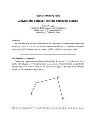
Geometric Modeling NotesANALYTIC DEFINITION OF A B-SPLINE CURVEKenneth I. JoyInstitute for Data Analysis and VisualizationDepartment of Computer ScienceUniversity of California, DavisOverviewSo, what will the analytic definition of the B-spline curve look like? The real question is whatwill the blending functions look like? Whereas the Bézier blending functions were the BernsteinPolynomials, which are extremely elegant and well-known, the B-spline blending functions are alittle messy. Here, we define the normalized B-spline blending functions N i,k (t), which enable usto write down an analytic definition of the B-spline curve.The B-Spline Curve – Analytical DefinitionA B-spline curve P(t), is defined bywhereP(t) =n∑P i N i,k (t) (1)i=0• the {P 0 , P 1 , ..., P n } are the control points,• k is the order of the polynomial segments of the B-spline curve. Order k means that thecurve is made up of piecewise polynomial segments of degree k − 1 – e.g., order 3 meansquadratic polynomial segments, and order 4 means cubic polynomial segments.• the N i,k (t) are the “normalized B-spline blending functions”. They are described by the orderk and by the knot sequence{t 0 , t 1 , t 2 , ..., t n+k } .

The N i,k (t) functions are described as follows⎧⎨1 if t ∈ [t i , t i+1 ),N i,1 (t) =⎩0 otherwise.(2)and if k > 1,N i,k (t) =t − t iN i,k−1 (t) +t i+k − tN i+1,k−1 (t) (3)t i+k−1 − t i t i+k − t i+1• and t ∈ [t k−1 , t n+1 ).This looks pretty complex, and it is “subscript-wise,” especially with Equation (3). It turns outthat the analytic definition of the B-spline curve is somewhat more complex than the geometricdefinition. However the analytic definition came first (for me, in a paper from 1949), and the geometricdefinition came later, from two researchers Carl DeBoor and Cox, working independently,in 1972. The DeBoor-Cox calculation started from the analytic definition, and derived the geometricdefinition, and we will use this method to show the equivalency of the geometric and analyticdefinitions.First, some bookkeeping...• There is some ambiguity in the definitions of the N .,. (t) blending functions. By defining themin a “recursive” manner. We must insure that in Equation (3), that if either of the N .,. termson the right hand side of the equation are zero, or the subscripts are out of the range of thesummation limits, then the associated fraction is not evaluated and the term becomes zero.This is to avoid a zero-over-zero evaluation problem.• We also note the “closed-open” interval [t k−1 , t n+1 ), which avoids some ambibuity whent = t n+1 .• The order k is independent of the number of control points (n + 1). With the Bézier curve,k = n, but in the B-Spline curve we have the flexibility of using many control points, andrestricting the degree of the polynomial segments that we piece together to make the finalcurve.2

It is also worthwhile to examine the blending functions carefully. Since they blend the control pointstogether, and B-splines are piecewise curves, we can conclude that the blending functions N i,k (t)must be non-zero only for a few values of i. This is easiest to see by “drawing” a few pyramids –math pyramids.If we draw the following dependency pyramid using Equation 3, [where various N .,. (t) functionsin the pyramid are a weighted sum of the two N .,. (t) functions immediately to its right]:N i,k (t)N i,k−1 (t)N i+1,k−1 (t)N i,1 (t)N i,2 (t). N i+1,1 (t). .. .N i,k−2 (t) .N i+1,k−2 (t)N i+2,k−2 (t) .. .. .. N i+k−2,1 (t)N i+k−1,2 (t)N i+k−1,1 (t)We can see that N i,k (t) (at the far left) eventually depends on N i,1 (t), N i+1,1 (t), ..., andN i+k−1,1 (t) (at the far right), and so we can conclude that N i,k (t) ≠ 0 only if t ∈ [t i , t i+k ). [Becauseif t ∉ [t i , t i+k ), then N i,1 (t), N i+1,1 (t), ..., and N i+k−1,1 (t) would all be zero).For each value of t, only a limited number of the N i,k (t) are non-zero.This can be seen by3

organizing a different pyramid. If t ∈ [t l , t k+1 ) then we can arrange the following pyramid.N l,1 (t)N l,2 (t)N l−1,2 (t)N l,k (t)N l−1,k−1 (t). N l−1,k (t). .. .N l,3 (t) .N l−1,3 (t)N l−2,3 (t) .. .. .. N l−k+2,k (t)N l−k+1,k−1 (t)N l−k+1,k (t)Here, the fact that N l,1 (t) ≠ 0 implies that N l,2 (t) ≠ 0 and N l−1,2 (t) ≠ 0 (the two blending functionsimmediately to its right in the pyramid) are also non-zero immediately to its right. And, in general,if N i,j (t) ≠ 0 implies that N i,j−1 (t) ≠ 0 and N i−1,j−1 (t) ≠ 0 in the pyramid. From this, we canconclude that if t ∈ [t l , t l+1 ), then only N l−k+1,k , N l−k+2,k , ..., and N l,k are non-zero. For example,N l−1,k (t) = N l−k,k (t) = 0.So, if t ∈ [t l , t l+1 ), only k of the N .,. functions are non-zero, and so only k of the control pointsP l−k+1 , P l−k+2 , ..., and P l affect the point P(t) on the curve. This makes sense, as a B-splinecurve is a piecewise polynomial curve, and only a few control points should affect eachpolynomial piece.So, if t ∈ [t l , t l+1 ), then we can rewrite Equation (1) to bel∑P(t) = P i N i,k (t) (4)i=l−k+1limiting the number of elements that must be considered in the sum – only k elements need to beconsidered.4

All contents copyright (c) 1997-2013Computer Science Department, University of California, DavisAll rights reserved.5