Magnus integrators for solving linear-quadratic differential ... - UPV

More documents

Recommendations

Info

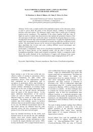
Author's personal copy3404 S. Blanes, E. Ponsoda / Journal of Computational and Applied Mathematics 236 (2012) 3394–3408Fig. 1. Error E [1] (t) = ∥H ex (t) − H [1] (t)∥ along the interval t ∈ [0, 1] for the choice c(t) = b e at and for different values of the parameters a and b.following we analyze the case: c = b e at for b ≥ 1, a > 0. In Fig. 1 we show the error E [1] (t) we take ∥A∥ = 1/2i,j A2 i,jalong the interval t ∈ [0, 1] for different values of the parameters a and b.Notice that, since c(t) ≥ 1 we can take a norm such that ∥K(t)∥ = c(t) and for a small value of a we have thatt∥K(tt 1 0)∥ dt 1 ∼ b, and we still have accurate results for b > π where the (sufficient but not necessary) convergencecondition (20) is not satisfied. We can also observe that the accuracy increases for small values of a, i.e. when c(t) is close toa constant (in this limit, the ME converges to the exact solution). Similar results are obtained taking for c(t) other smoothfunctions.Example 4. In [41] a problem of air pollutant emissions from two regions is proposedx ′ (t) = −ax(t) + bu 1 (t) + bu 2 (t); x(0) = x 0 . (36)Here x(t) is the excess of the pollutant in the atmosphere, u i (t), i = 1, 2, denotes the emissions of each region and a, b arepositive constants related with the intervention of the nature on environment. The cost functions to minimize are given byJ i = 1 2 T0e −ρt c i u 2 i (t) + d ix 2 (t) dt, i = 1, 2, (37)where c i , d i , are positive parameters related to the costs of emission and pollution withstand respectively, and ρ is a refreshrate. With an appropriate change of constants, the problem (36) and (37) can be applied to other situations, such as financialproblems for example, see [4].In our notation, Q iT = 0, i = 1, 2, R ij = 0, i ≠ j, Q i (t) = d i e −ρt , R ii = c i e −ρt , and S i = b 2 e ρt /c i , i = 1, 2.We generalize this problem to the case of N regions (N players) where the Eq. (36) changes tox ′ (t) = −ax(t) + bNu i (t); x(0) = x 0 ,i=1and the index for the remaining parameters range for i = 1, . . . , N. Then, following the steps indicated at the end ofSection 2.1, we have:• the Eq. (15) with the datay ′ (t) = K(t)y(t), y(T) = [1, 0, . . . , 0] T ;
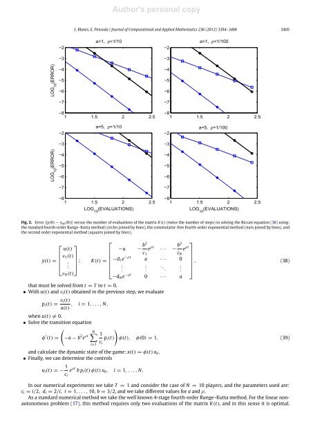
Author's personal copyS. Blanes, E. Ponsoda / Journal of Computational and Applied Mathematics 236 (2012) 3394–3408 3405Fig. 2. Error ∥y(0) − y ap (0)∥ versus the number of evaluations of the matrix K(t) (twice the number of steps) in solving the Riccati equation (38) using:the standard fourth-order Runge–Kutta method (circles joined by lines), the commutator-free fourth-order exponential method (stars joined by lines), andthe second order exponential method (squares joined by lines).⎡ ⎤u(t)v 1 (t)y(t) = ⎢⎥⎣. ⎦ ;v N (t)⎡⎤−a − b2e ρt · · · − b2e ρtc 1 c N K(t) = −d 1 e −ρt a · · · 0, (38)⎢⎣... ... ..⎥⎦−d N e −ρt 0 · · · athat must be solved from t = T to t = 0.• With u(t) and v i (t) obtained in the previous step, we evaluatep i (t) = v i(t), i = 1, . . . , N,u(t)when u(t) ≠ 0.• Solve the transition equationNφ ′ (t) = −a − b 2 e ρt 1p i (t) φ(t), φ(0) = 1, (39)c ii=1and calculate the dynamic state of the game: x(t) = φ(t) x 0 .• Finally, we can determine the controlsu i (t) = − 1 c ie ρt b p i (t) φ(t) x 0 , i = 1, . . . , N.In our numerical experiments we take T = 1 and consider the case of N = 10 players, and the parameters used are:c i = i/2, d i = 2/i, i = 1, . . . , 10, b = 3/2, and we take different values for a and ρ.As a standard numerical method we take the well known 4-stage fourth-order Runge–Kutta method. For the linear nonautonomousproblem (17), this method requires only two evaluations of the matrix K(t), and in this sense it is optimal.
Page 3 and 4: Author's personal copyS. Blanes, E.
Page 6 and 7: Author's personal copy3398 S. Blane
Page 16: Author's personal copy3408 S. Blane

Magnus integrators for solving linear-quadratic differential ... - UPV

Create successful ePaper yourself

Delete template?

Save as template?