Report: Assignment #1 Course: CAP 5400 – Digital Image ...

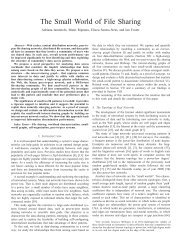
Image 8: T=15, W=7x7 Image 9: T=15, W=9x9 Image 10: T=15, W=11x11It seems that the variable thresholding operation performs a kind of edge detection which is morepronounced for larger window sizes. This is because it in effect converts to white all the pixelsthat are above a limit larger than their neighboring, which in turn occurs usually in edges. Thefollowing images are from a picture of 5 cubes. The window size is kept constant and thethreshold parameter is changed gradually from 3 to 9. The operation is carried out in a regionthat contains only the cubes and not the background.Image 11: Original photo of cubes (scaled down)Image 12: T=3, W=5x5, ROI=(40,30,300,200)Image 14: T=5, W=5x5, ROI=(40,30,300,200)Image 13: T=9, W=5x5, ROI=(40,30,300,200)

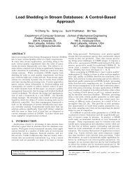
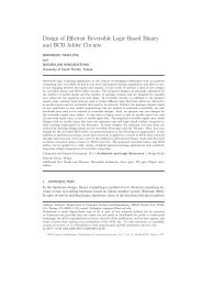
353025Time (msec)201510500 50 100 150 200 250 300 350 400N^2 (Kpixel)Chart 1: Pixel averaging performance as a function ofimage sizeIt is evident that we have at most two nested loops that cover at most the whole image, thereforethe computational complexity of the algorithm is O N 2 . Of course the algorithm is slower thanregular thresholding since we have to execute the nested loops 4 times (incremental averaging ony axis, incremental averaging on x axis, normalization and thresholding). We also have tocompute the first row and column to apply the incremental averaging.In addition to that the memory requirements are larger because the regular thresholding can beapplied in place since the algorithm is a point operation. On the other hand the variablethresholding is a local operation and therefore needs three times as much memory to store theintermediate temporary image and the final averaged image, that will be later used for thethresholding itself.3.4. Color binarizationThe set of pictures on the following page, illustrates the operation of color binarization. Theoriginal image is being thresholded against the red, green and blue colors. With a low threshold(T=50) the algorithm clearly separates the red, green and blue parts of the image and convertsthem to black while the rest are turned to white.Unfortunately for larger values of threshold (T=250) the separation is not so good and includessome pixels with intermediate values, which some times are not the ones expected. For exampleby increasing the threshold on the red binarization operation, we got several pixels that weresituated at the borders of the blue and green colors, while someone would expect that theadditional pixels would be from the regions where the colors blend with each other. Also regionsthat appeared to have no color, like the black letters, where also included in the binarized image.A border was placed after the processing on each image so that their boundaries are clearlydefined.

Image 15:Original RGBpictureImage 16:T=50,C=(255,0,0)Image 17:T=50,C=(0,255,0)Image 18:T=50,C=(0,0,255)Image 19:T=250,C=(255,0,0)Image 20:T=250,C=(0,255,0)Image 21:T=250,C=(0,0,255)In the photos below the color binarization was applied successfully to separate the oranges fromthe background. The algorithm was performed in a region of interest that contains only theoranges, so the plate is left untouched. The last set present the separation of the blue sea starsusing color binarization.Image 22: Original photo of oranges (scaled down)Image 23: T=100, C=(255,125,0),ROI=(75,45,260,160)Image 24: Original photo of seastarsImage 25: T=200, C=0,0,255

3.5. Performance of the color binarization algorithmIn order to assess the performance of the color binarization algorithm, a test was carried outusing the same image in the following sizes: 600x600, 500x500, 400x400, 300x300 and200x200. The algorithm applied the color binarization algorithm to each of these images 100times and the resulting time was divided by 100. The following graph shows the time for eachimage size (N). From Chart 2, it is evident that the execution time of the algorithm dependslinearly on the N 2 .The color binarization algorithm is about 20% faster than the variable thresholding operation andabout 4 times slower than the regular thresholding. This is due to the fact that for each pixel thecolor binarization algorithm needs to compute the euclidean distance in 3D space before eachcomparison to the threshold.Time (msec)4540353025201510500 50 100 150 200 250 300 350 400N^2 (Kpixel)Chart 2: Color binarization performance as a functionof image size