A simple method of generating equations of state for hard sphere fluid

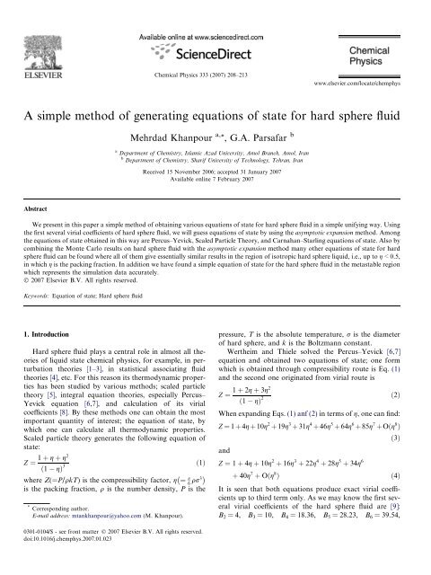
Chemical Physics 333 (2007) 208–213www.elsevier.com/locate/chemphysA simple method of generating equations of state for hard sphere fluidMehrdad Khanpour a, *, G.A. Parsafar ba Department of Chemistry, Islamic Azad University, Amol Branch, Amol, Iranb Department of Chemistry, Sharif University of Technology, Tehran, IranReceived 15 November 2006; accepted 31 January 2007Available online 7 February 2007AbstractWe present in this paper a simple method of obtaining various equations of state for hard sphere fluid in a simple unifying way. Usingthe first several virial coefficients of hard sphere fluid, we will guess equations of state by using the asymptotic expansion method. Amongthe equations of state obtained in this way are Percus–Yevick, Scaled Particle Theory, and Carnahan–Starling equations of state. Also bycombining the Monte Carlo results on hard sphere fluid with the asymptotic expansion method many other equations of state for hardsphere fluid can be found where all of them give essentially similar results in the region of isotropic hard sphere liquid, i.e., up to g < 0.5,in which g is the packing fraction. In addition we have found a simple equation of state for the hard sphere fluid in the metastable regionwhich represents the simulation data accurately.Ó 2007 Elsevier B.V. All rights reserved.Keywords: Equation of state; Hard sphere fluid1. IntroductionHard sphere fluid plays a central role in almost all theoriesof liquid state chemical physics, for example, in perturbationtheories [1–3], in statistical associating fluidtheories [4], etc. For this reason its thermodynamic propertieshas been studied by various methods; scaled particletheory [5], integral equation theories, especially Percus–Yevick equation [6,7], and calculation of its virialcoefficients [8]. By these methods one can obtain the mostimportant quantity of interest; the equation of state, bywhich one can calculate all thermodynamic properties.Scaled particle theory generates the following equation ofstate:Z ¼ 1 þ g þ g2ð1Þð1 gÞ 3where Z(=P/qkT) is the compressibility factor, g ¼ p qr3 6is the packing fraction, q is the number density, P is the* Corresponding author.E-mail address: mtankhanpour@yahoo.com (M. Khanpour).pressure, T is the absolute temperature, r is the diameterof hard sphere, and k is the Boltzmann constant.Wertheim and Thiele solved the Percus–Yevick [6,7]equation and obtained two equations of state; one formwhich is obtained through compressibility route is Eq. (1)and the second one originated from virial route is1 þ 2g þ 3g2Z ¼ ð2Þð1 gÞ 2When expanding Eqs. (1) anf (2) in terms of g, one can find:Z ¼ 1 þ 4g þ 10g 2 þ 19g 3 þ 31g 4 þ 46g 5 þ 64g 6 þ 85g 7 þ Oðg 8 Þð3ÞandZ ¼ 1 þ 4g þ 10g 2 þ 16g 3 þ 22g 4 þ 28g 5 þ 34g 6þ 40g 7 þ Oðg 8 ÞIt is seen that both equations produce exact virial coefficientsup to third term only. As we may know the first severalvirial coefficients of the hard sphere fluid are [9]:B 2 =4, B 3 = 10, B 4 = 18.36, B 5 = 28.23, B 6 = 39.54,ð4Þ0301-0104/$ - see front matter Ó 2007 Elsevier B.V. All rights reserved.doi:10.1016/j.chemphys.2007.01.023

M. Khanpour, G.A. Parsafar / Chemical Physics 333 (2007) 208–213 209B 7 = 53.54 and B 8 = 70.78. Carnahan and Starling used thefirst three virial coefficients (of course they adoptedB 4 = 18) and approximated the virial coefficients to beB n = n 2 +3n and summed the virial coefficients, thenreached to their famous equation [10]:Z ¼ g3 g 2 g 1ðg 1Þ 3 ð5ÞAnother route to obtain hard sphere fluid equations ofstate stems from virial expansion. Summing the known firstseveral virial coefficients of the hard sphere fluid by, say,Padé approximation method, one may obtain some equationsof state. For example, Ree and Hoower found the followingequation [11]:Z ¼ 1 þ 1:75399g þ 2:31704g2 þ 1:108928g 31 2:246004g þ 1:301056g 2 ð6ÞAlso one can employ the so-called rescaled virial expansionto obtain equations of state for hard spheres [12,13].Here we present a simple method to generate manyequations of state (among them are Eqs. (1), (2) and (5))for hard sphere fluid.2. The asymptotic expansion methodWe start from known virial coefficients of hard spherefluid and writeZ ¼ 1 þ B 2 g þ B 3 g 2 þ B 4 g 3 þWe may notice that if Eq. (7) should represent the propertiesof a real fluid, it must be convergent. Suppose the radiusof convergence of the virial expansion is b; thereforeg must be less than b, because for g P b the virial expansionbecomes divergent, i.e., it can not represent a real system.Since we are unable to obtain and calculate all virialcoefficients, we can only hope to obtain an approximation.By now, all that we know besides knowing first several virialcoefficients is that it must be divergent at g P b. So onecan deduce that b is a pole for the compressibility factorZ = Z(g). Taking this fact into account we may write theasymptotic expansion of Z, which is of the form:ð7ÞZ ¼ a 0 þ a 1g b þ a 2ðg bÞ þ a 3þ ... ð8Þ2 3ðg bÞAdopting this form for the asymptotic expansion of Z, thenexpanding into virial form and comparison with knownfirst several virial coefficients, one can easily arrive at muchmany equations of state for hard sphere fluid, all of themare in fact asymptotic forms of Z.3. Some equations of state for hard sphere fluidSince we are not aware of the exact value of b at whichthe virial expansion, Eq. (7), becomes divergent, we are freeto choose it conveniently. Because hard spheres crystallizeat g = 0.7405 [9], hence one may assume any value for bgreater than 0.7405, say, b = 3/4, b =1, or b = 2, besidesthis we can not say anymore. In addition to this, the numberof terms in asymptotic expansion, Eq. (8), is anotherdegree of freedom we have. For example, if we restrict ourselvesto use only three known virial coefficients, we shouldselect those asymptotic forms with only three unknowns.But if one would like to find more rigorous representationsfor equation of state, (s)he should know and use more virialcoefficients, hence more possibilities for the form ofasymptotic expansion are there to be tried. As we maysee, virial coefficients are all related to b, the pole (see forexample Eq. (10)). As soon as selecting a definite valuefor b, one is able to obtain the desired coefficients. Differentb’s produce different coefficients, but up to third order ofcourse, they are all the same. They approximate differentvalues for the remainder terms. Among them one mustbe the best, but this method can not achieve this importantgoal alone. At the best we can resort to approximate theorieslike Scaled Particle Theory which asserts that b =1,orapproximately determine it by the known virial coefficientsas done in Section 4.(A) Suppose that the asymptotic form of the compressibilityfactor Z to be:Z ¼ a 0 þ a 1g b þ a 2ð9Þðg bÞ 2Expanding Eq. (9) in powers of g gives:a 1Z ¼ a 0b þ a 2 a 1þb 2 b þ 2a 2g2 b 3a 1þb þ 3a 2g 2 þ Oðg 3 Þð10Þ3 b 4By equating these coefficients with known second and thirdvirial coefficients gives:8>< a 0 a 1 =b þ a 2 =b 2 ¼ 1a 1 =b 2 þ 2a 2 =b 3 ¼ B 2ð11Þ>:a 1 =b 3 þ 3a 2 =b 4 ¼ B 3Which its solution is:8>< a 0 ¼ 1 2B 2 b þ B 3 b 2a 1 ¼ 3B 2 b 2 þ 2B 3 b 3>:a 2 ¼ B 2 b 3 þ B 3 b 4ð12ÞInserting these values in Eq. (9) and collecting we finallyobtain:Z ¼ ð1 2B2b þ B3b2 Þg 2 þðB2b 2 2bÞg þ b 2ð13Þðg bÞ 2Now we may put b = 1(together with B 2 = 4 and B 3 = 10)in Eq. (13) which gives:Z ¼ 3g2 þ 2g þ 1ð14Þðg 1Þ 2

210 M. Khanpour, G.A. Parsafar / Chemical Physics 333 (2007) 208–213This is the well-known equation of state of Wertheim andThiele, Eq. (2), obtained from the analytical solution ofthe Percus–Yevick equation by the virial route.(B) Now we suppose that the asymptotic form of thecompressibility factor Z to be (while retaining theunknowns to be three again since we want to use onlyfirst two virial coefficients as in previous example):Z ¼ a 1g b þ a 2ðg bÞ 2 þ a 3ðg bÞ 3 ð15ÞBy taking similar steps one finds:Z ¼ bðð3 3B2b þ B3b2 Þg 2 þðB2b 2 3bÞg þ b 2 Þðg bÞ 3 ð16ÞNow putting b = 1 (together with B 2 = 4 and B 3 = 10) inEq. (16) gives:Z ¼ g2 þ g þ 1ð1 gÞ 3 ð17ÞThis is the well-known equation of state of Scaled ParticleTheory, Eq. (1) and also obtained from the analytical solutionof the Percus–Yevick equation by the compressibilityroute.(C) In order to obtain another (proposed originally in[14]) equation of state we suppose that the asymptoticform of Z is:Z ¼ a 0 þ a 1g 3=4 þ a 2ð18Þg 1where we have used two values for b; i.e., b = 1 and b = 3/4that come from Scaled Particle Theory and close packingfraction of hard spheres [9], respectively. Proceeding as beforewe will find the following equation:Z ¼ 6g2 þ 5g þ 3ð19Þð4g 3Þðg 1ÞThis equation has been used for simplification of SAFTequation of state for hard sphere chains [15,16].(D) Now we proceed one step further and suppose thatthe asymptotic form of Z is:Z ¼ a 0 þ a 1g b þ a 2ðg bÞ þ a 3ð20Þ2 ðg bÞ 3We have this time four unknowns, hence need to employup to fourth virial coefficients. For simplicity we setB 4 = 18 as Carnahan and Starling did and proceed as beforeto obtain:Z ¼ðð28b 4 þ 1 16b þ 60b 2 72b 3 Þg 3 þð20b 3 3b54b 4 þ 28b 5 þ 8b 2 Þg 2 þð3b 2 54b 5 þ 28b 6þ 30b 4 8b 3 Þg b 3 4b 4 þ 30b 5 54b 6þ 28b 7 Þ=ðg bÞ 3 ð21ÞNow if we set b = 1 in Eq. (21) we arrive at the well-knownCarnahan–Starling equation:Z 22 ¼ g3 g 2 g 1ð22Þðg 1Þ 3(E) In this stage we would like to improve the Carnahan–Starling equation a bit further by taking the exactvalue of the fourth virial coefficient, i.e., B 4 = 18.36and employ Eq. (20) to obtain a new approximationfor Z. Doing as before we obtain:Z ¼ ð 30b2 þ 12b 1 þ 18:36b 3 Þg 3 þð10b 3 12b 2 þ 3bÞg 2 þð4b 3 3b 2 Þg þ b 3ð g þ bÞ 3 ð23ÞNow if we set b = 1 in Eq. (23) we arrive at the followingequation:Z 24 ¼ 0:64g3 g 2 g 1ð24Þðg 1Þ 3(F) It is obvious that if we take some other values for bwe will find another set of equations for hard spherefluid. For example, by inserting b = 3/4 in Eqs. (13),(16), (21), and (23), respectively, one finds:Z 25 ¼ 10g2 þ 12g þ 9ð4g 3Þ 2 ð25ÞZ 26 ¼ 9ð2g2 3Þð26Þð4g 3Þ 3Z 27 ¼ 82g3 þ 18g 2 27ð4g 3Þ 3 ð27ÞZ 28 ¼ 72:28g3 þ 18g 2 27ð28Þð4g 3Þ 3(G) One may also prefer another choice for the asymptoticexpansion of Z, for instance, we may supposethe following form:Z ¼ a 0 þ a 1g34þ a 2ðg bÞ 2 þ a 3ðg bÞ 3 ð29ÞWe therefore will need to have four virial coefficients wherewe take B 4 = 18 for simplicity. Proceeding as before wefind the following equation:Z ¼ 81b 3 144b 4 þ 72b 5 81g 3 216g 4 243b 2 gþ 648b 3 g 600b 4 g þ 243bg 2 þ 888bg 4 2358b 2þ 1746b 3 g 2 þ 792bg 3 1080b 2 g 2 1137b 2 g 4 þ 2970b 3 g 31248b 4 g 2 þ 192b 5 g þ 588b 3 g 4 1680b 4 g 3 þ 336b 5 g 2112b 4 g 4 þ 336b 5 g 3 = 38b 2 16b þ 9 ð4g 3Þð g þ bÞ 3ð30ÞNow we set, say, b = 3/2 to obtain the following equation:Z 31 ¼ 22g4 þ 114g 3 54g 2 54g 81ð4g 3Þð2g 3Þ 3 ð31Þ

M. Khanpour, G.A. Parsafar / Chemical Physics 333 (2007) 208–213 2114. Determination of the radius of convergence from the virialcoefficientsUntil now, the choice of the radius of convergence (b)was arbitrary. But we can determine b from the virial coefficients;hence there is indeed no need to assume it freely. Itis obvious that if we take b as another unknown, we areable to find it. Also we would like to work with only threeknown virial coefficients, i.e., B 2 =4,B 3 = 10, B 4 = 18.36,hence we prefer to work with Eqs. (9) and (15).I. First we work with Eq. (9) and write it:Z ¼ a 0 þ a 1g b þ a 2ðg bÞ 2 ð32Þwhich may be expanded in powers of g up to fourth order:a 1Z ¼ a 0b þ a 2þ 2a 2 a 1g þ 3a 2 a 1g 2b 2 b 3 b 2 b 4 b 3þ 4a 2 a 1g 3 þ Oðg 4 Þð33Þb 5 b 4Equating these coefficients with known first three virialcoefficients gives:8a 0 a 1 =b þ a 2 =b 2 ¼ 1>< 2a 2 =b 3 a 1 =b 2 ¼ 4ð34Þ3a 2 =b 4 a 1 =b 3 ¼ 10>:4a 2 =b 5 a 1 =b 4 ¼ 18:36This system of equations has two set of solutions.The firstset is:b ¼ 0:26; a 0 ¼ 0:41; a 1 ¼ 0:47; a 2 ¼ 0:03and the second one:b ¼ 0:83; a 0 ¼ 1:21; a 1 ¼ 3:07; a 2 ¼ 2:39 ð35ÞSince we would like to have b as large as possible we mustchoose the second set. Inserting these values in Eq. (32) andcollecting them gives the desired equation:Z 36 ¼ 1:21g2 þ 1:07g þ 0:68ð36Þðg 0:83Þ 2II. As the second step we invoke Eq. (15) and write it:Z ¼ a 1g b þ a 2ðg bÞ 2 þ a 3ðg bÞ 3 ð37Þwhich may be expanded in powers of g up to fourth order:a 1Z ¼b þ a 2 a 3 3a 3 a 1þb 2 b 3 b 4 b þ 2a 2g2 b 36a 3þb þ 3a 2 a 1g 2 þ 4a 2 10a 3 a 1g 35 b 4 b 3 b 5 b 6 b 4þ O g 4ð38ÞEquating these coefficients with known first three virialcoefficients gives:8a 1 =b þ a 2 =b 2 a 3 =b 3 ¼ 1>:4a 2 =b 5 10a 3 =b 6 a 1 =b 4 ¼ 18:36This system of equations has three set of solutions.The firsttwo sets are:a 2 ¼ 0:01; a 3 ¼ 0; b ¼ 0:11; a 1 ¼ 0:20a 3 ¼ 0:05; a 2 ¼ 0:39; b ¼ 0:45; a 1 ¼ 0:17These are rejected in favor of the third set:a 2 ¼ 5:20; a 3 ¼ 4:81; b ¼ 1:07; a 1 ¼ 1:74 ð40ÞThis is our desired solution because b in this solution hasthe greatest value. Inserting these values in Eq. (37) andcollecting them gives the desired equation:Z 41 ¼ 1:74g2 þ 1:48g þ 1:23ð41Þðg 1:07Þ 3III. As our final example we use Eq. (20):Z ¼ a 0 þ a 1g b þ a 2ðg bÞ 2 þ a 3ðg bÞ 3 ð42Þwhich may be expanded in powers of g up to fifth order:a 1Z ¼ a 0b þ a 2 a 3 a 1þb 2 b 3 b þ 2a 2 3a 3g2 b 3 b 4a 1þb þ 3a 2 6a 3g 2 þ a 13 b 4 b 5 b þ 4a 2 10a 3g 34 b 5 b 6a 1þb þ 5a 2 15a 3g 4 þ O g 5ð43Þ5 b 6 b 7Equating these coefficients with known virial coefficients(where for simplicity we set B 4 =18andB 5 = 28 as Carnahanand Starling did) gives:8a 0 a 1 =b þ a 2 =b 2 a 3 =b 3 ¼ 1>< a 1 =b 2 þ 2a 2 =b 3 3a 3 =b 4 ¼ 4a 1 =b 3 þ 3a 2 =b 4 6a 3 =b 5 ¼ 10ð44Þa 1 =b 4 þ 4a 2 =b 5 10a 3 =b 6 ¼ 18>:a 1 =b 5 þ 5a 2 =b 6 15a 3 =b 7 ¼ 28This system of equations has two set of solutions, the firstset reads:b ¼ 0:19; a 0 ¼ 0:33; a 1 ¼ 0:40; a 2 ¼ 0:03;a 3 ¼ 0that should be rejected in favor of the following one:a 0 ¼ 1; b ¼ 1; a 1 ¼ 2; a 2 ¼ 0; a 3 ¼ 2Not surprisingly, when putting them in Eq. (42) the famousCarnahan–Starling equation (Eq. (5)) will be recovered.Wemay compare the obtained equations of state for hardsphere fluid to computer simulation data, too. For this pur-

212 M. Khanpour, G.A. Parsafar / Chemical Physics 333 (2007) 208–213( Z - Z MC) / Z MC0.10.080.060.040.020-0.02Δ Z 22Δ Z 24Δ Z 27Δ Z 28Δ Z 31Δ Z 36Δ Z 41( Z - Z MC) / Z MC8 x 10-36420-2Δ Z 45Δ Z 46Δ Z 47Δ Z 22-0.04-0.060.05 0.1 0.15 0.2 0.25 0.3 0.35 0.4 0.45 0.5ηFig. 1. Relative deviation curves of the obtained hard sphere equations ofstate based on known virial coefficients with computer simulation data.pose we have used the computer simulation data from [17].The results are shown in Fig. 1. We may easily observe thatall obtained equations can essentially well represent thehard sphere fluid properties in the isotropic liquid range,i.e., when g 6 0.5. In addition we have compared the virialcoefficients of the obtained equations of state with the exactvalues in Table 1.5. Equations of state based on computer simulation dataIn previous sections one restricted to use only knownvirial coefficients. Suppose we have access to computer simulationdata. Since asymptotic expansion method produceas essentially accurate results as the original function, wemay expect that (the various forms of) Eq. (8) can be usedto accurately represent the original data. For this purposewe may use the recent Monte Carlo reported in Ref. [17]for hard sphere fluid in two cases; i.e., isotropic liquidand metastable fluid regions.5.1. The isolated liquid regionWe choose the asymptotic form of the compressibilityfactor Z to be like Eq. (20). Fitting the MC data by thatequation and collecting, one finds:-4-60 0.10.2 0.3 0.4 0.5ηFig. 2. Relative deviation curves of the obtained hard sphere equations ofstate based on Monte Carlo results with Carnahan–Starling and computersimulation data.Z 45 ¼ 1:714g3 þ 0:014g 3 0:161g 0:542ð45Þðg 0:814Þ 3One may also suppose in Eq. (20) that b = 1, and then performfitting to obtain:Z 46 ¼ 1:151g3 1:088g 2 0:990g 1:003ðg 1Þ 3 ð46ÞIt is interesting to notice the very similarity between thisequation with the Carnahan–Starling’s.Another suitable choice is to use Eq. (9), which after fittingwith MC data gives:Z 47 ¼ 2:508g2 þ 1:326g þ 0:825ðg 0:903Þ 2 ð47ÞA comparison of these equations and Carnahan–Starlingequation with MC data in the isotropic liquid region hasbeen made in Fig. 2. As can be seen they are all essentiallythe same in this region. In addition we have compared thevirial coefficients of the obtained equations of state with theexact values in Table 1.Table 1Comparison of the virial coefficients of the obtained hard sphere equations of state with computer simulation dataaVirial coefficients Z MD Z 22 Z 24 Z 27 Z 28 Z 31 Z 36 Z 41 Z 45 Z 46 Z 47B 2 4 4 4 4 4 4 4 4 3.99 3.99 3.87B 3 10 10 10 10 10 10 10 10 10.143 10.08 10.40B 4 18.36 18 18.36 18 18.36 18 18.36 18.36 17.99 18.08 18.28B 5 28.23 28 29.08 28.15 29.59 27.63 29.81 28.53 27.78 28.02 27.74B 6 39.54 40 42.16 40.30 44.14 39.26 45.28 40.03 39.75 39.89 39.02B 7 53.54 54 57.60 53.73 62.26 53.73 65.97 52.45 54.06 53.69 52.40B 8 70.78 70 75.40 66.72 83.79 72.25 93.38 65.45 70.79 69.41 68.21B 9 93.06 88 96.56 75.85 107.71 96.44 129.44 78.73 89.83 87.07 86.80B 10 123.21 108 118.08 74.9 131.55 128.38 176.59 92.06 110.79 106.66 108.59a Taken from Ref. [9].

M. Khanpour, G.A. Parsafar / Chemical Physics 333 (2007) 208–213 213( Z - Z MC) / Z MC0.10-0.1-0.2-0.3-0.4-0.5-0.6-0.7Δ Z 22Δ Z 47Z ¼ a 0 þ a 1ð49Þg bFitting the MC data in this region and collecting, one finds:3:730g 3:712Z 50 ¼ ð50Þg 0:642Comparison between these two equations in Fig. 4 revealsthat Eq. (50) represents MC data in the metastable regioneven better than Eq. (48). Of course, if one wants, it is possibleto obtain more accurate equation by using, say, Eq.(9), but it will not be as simple as Eq. (50).-0.8-0.90 0.1 0.2 0.3 0.4 0.5 0.6 0.7ηFig. 3. Relative deviation curves of Eqs. (47) and (22) with computersimulation data in the whole liquid region of hard sphere fluid.( Z - Z MC) / Z MC0.150.10.050-0.05-0.1-0.15-0.2-0.25-0.3Δ Z 48Δ Z 50-0.350.5 0.52 0.54 0.56 0.58 0.6 0.62 0.64Fig. 4. Relative deviation curves of Eqs. (48) and (50) with computersimulation data in the metastable region of hard sphere fluid.Eq. (47) appears to be interesting, because it is simplerthan the others. In Fig. 3 a comparison has been madebetween Eq. (47) and Carnahan–Starling equation in thewhole liquid region of hard sphere fluid which indicate thatthey give essentially the same results in the liquid region ofhard sphere fluid.5.2. The metastable fluid regionSpeedy [18] has given a purely empirical equation for themetastable fluid region:2:67Z 48 ¼ð48Þ1 1:543gSo we choose the simplest form of asymptotic expansion torepresent this region; i.e.,η6. ConclusionWe have presented in this paper a simple method ofobtaining various equations of state for hard sphere fluidin a simple unifying way. Using the first several virial coefficientsof hard sphere fluid, we will guess equations of stateby using the asymptotic expansion method. Among theequations of state obtained in this way are Percus–Yevick,Scaled Particle Theory, and Carnahan–Starling equationsof state. Also by combining the Monte Carlo results onhard sphere fluid with the asymptotic expansion methodmany other equations of state for hard sphere fluid canbe found where all of them give essentially similar resultsin the region of isotropic hard sphere liquid, i.e., up tog < 0.5, in which g is the packing fraction. In addition wehave found a simple equation of state for the hard spherefluid in the metastable region which represents the simulationdata accurately.References[1] J.A. Barker, D. Henderson, J. Chem. Phys. 47 (11) (1967) 4714.[2] J.D. Weeks, D. Chandler, H.C. Andersen, J. Chem. Phys. 54 (1971)5237.[3] S. Jiuxun, C. Lingcang, W. Qiang, J. Fuqian, Physica A 326 (2003)482.[4] P. Paricaud, A. Galindo, G. Jackson, Fluid Phase Equilibr. 194–197(2002) 87.[5] H. Reiss, H.L. Frisch, J.L. Lebowitz, J. Chem. Phys. 31 (1959) 369.[6] M.S. Wertheim, Phys. Rev. Lett. 10 (1963) 321.[7] E. Thiele, J. Chem. Phys. 39 (1963) 474.[8] A. Santos, S.B. Yuste, M. Lòpez de Haro, Mol. Phys. 99 (23) (2001)1959.[9] L.V. Yelash, T. Kraska, Phys. Chem. Chem. Phys. 3 (2001) 3114.[10] N.F. Carnahan, K.E. Starling, J. Chem. Phys. 51 (1969) 635.[11] F.H. Ree, W.G. Hoover, J. Chem. Phys. 40 (1964) 939.[12] M. Baus, J.L. Colot, Phys. Rev. A 36 (8) (1987) 3912.[13] A. Malijevsky, J. Veverka, Phys. Chem. Chem. Phys. 1 (1999) 4267.[14] L.V. Yelash, T. Kraska, U.K. Deiters, J. Chem. Phys. 110 (1999)3079.[15] L.V. Yelash, T. Kraska, Phys. Chem. Chem. Phys. 1 (1999) 2449.[16] L.V. Yelash, T. Kraska, E.A. Müller, N.F. Carnahan, Phys. Chem.Chem. Phys. 1 (1999) 4919.[17] G.-W. Wu, R.J. Sadus, AIChE J. 51 (2005) 309.[18] R.J. Speedy, J. Chem. Phys. 100 (1994) 6684.