S.C.Geller et al.regression techniques, or the program dChip, which usesan iterative procedure with regression <strong>and</strong> outlier detection(http://www.dchip.org; Li <strong>and</strong> Wong, 2001). Thenegative values for intensities (e.g. when MM > PM) causeproblems when the commonly used log transform is applied tothe normalized <strong>data</strong>. Also, if the variance is not constant acrossexpression levels, then the mean chip/slide intensity is not anoptimal measure <strong>of</strong> the overall level <strong>of</strong> a given chip/slide.We will demonstrate that <strong>data</strong> from Affymetrix GeneChipsconform at least approximately to the two-component model<strong>of</strong> error. Then we shall provide a procedure by which to findthe transformation constant c <strong>and</strong> normalize the <strong>data</strong> at thesame time. This simultaneous procedure is necessary underthe assumptions <strong>of</strong> our model. This method avoids many<strong>of</strong> the problems <strong>of</strong> alternative <strong>normalization</strong> <strong>and</strong> transformationmethods. In particular there is no problem with negativeobserved intensities.2 DATAIn order to investigate replicability <strong>and</strong> the appropriateness <strong>of</strong>the two-component model <strong>of</strong> error for <strong>data</strong> from Affymetrixchips, a single lymphoblastoid cell line from one autistic childwas grown in four separate T75 flasks. The cells were splitfrom the same parent flask <strong>and</strong> grown in the same incubator,same shelf, at the same time. Four separate RNA extractionswere performed when the cells were near confluence. cDNAsynthesis <strong>and</strong> in vitro transcription (IVT) labeling were performedon each sample. Each sample was then hybridizedto an Affymetrix Human Genome U95Av2 <strong>oligonucleotide</strong>GeneChip array, which contains 12 625 probe sets, with eachprobe set designed to represent a single human gene. Notethat these are true replicates <strong>of</strong> the whole measurement process,not just machine replicates in which the same sampleafter processing is divided <strong>and</strong> hybridized to several differentchips. †This study is part <strong>of</strong> a larger project to investigate thegenetic basis <strong>of</strong> autism, a behavioral diagnosis that reflectscomplex <strong>and</strong> ill-defined patterns <strong>of</strong> inheritance <strong>and</strong> possibleenvironmental factors. Although autism is highly heritable,with over 90% concordance for autism spectrum disorders,genome-wide linkage studies have been unable to definespecific chromosomal loci for the preponderance <strong>of</strong> autisticindividuals, excluding known genetic disorders [e.g. Rett syndrome,fragile X syndrome, tuberous sclerosis, 15q(dup)]that have autistic features as a variable component <strong>of</strong> their†There are a number <strong>of</strong> differing types <strong>of</strong> replicates depending on wherein the process one starts. A fundamental assumption <strong>of</strong> our model is thatthe replicates used to estimate it come from the same biological sample forall replicates in a group. Thus, we are considering measurement error, notvariability within <strong>and</strong> between organisms. The samples we are using for thispaper all come from the same cell line. We are measuring, in this case, all<strong>of</strong> the sources <strong>of</strong> error beginning with the collection <strong>of</strong> the cells, throughhybridizing to the chip <strong>and</strong> reading the results.phenotypes. An alternative approach to the identification <strong>of</strong>genetic components <strong>of</strong> autism, including those conferringdifferential susceptibility to putative environmental factors,is the identification <strong>of</strong> patterns <strong>of</strong> altered gene expressionthrough <strong>microarray</strong> methods. This approach entails the analysis<strong>of</strong> blood <strong>and</strong> tissue samples from autistic patients <strong>and</strong>unaffected family members with the objective <strong>of</strong> identifyingpatterns <strong>of</strong> gene expression that associate with the autism spectrumphenotype. Information derived from such investigationswould be <strong>of</strong> critical importance for both predictive efforts(which children are at increased risk to develop autism) <strong>and</strong>efforts to define the various biochemical/genetic mechanismsthat lead to autism.All graphs <strong>and</strong> computed statistics in this paper are fromthe <strong>data</strong> set <strong>of</strong> Perfect Match (PM)/ Mismatch (MM) differencesfor 12 625 genes for four replicates or flasks. We usedthe average difference (PM–MM) <strong>data</strong> as they are reportedby Microarray Suite 4.0 (MAS 4.0; Affymetrix Inc.) withoutusing their <strong>normalization</strong> program. Version 4 reports negativevalues when the MM is greater than the PM. §Since the st<strong>and</strong>ard deviation <strong>of</strong> the low expression level<strong>data</strong> is approximately 8, we considered genes for which themedian value <strong>of</strong> the four replicates was less than or equal to−25 to be unusable outliers, <strong>and</strong> eliminated those 655 genes.In general the <strong>data</strong> can be thought <strong>of</strong> as an n × m array <strong>of</strong>intensity levels where n is the number <strong>of</strong> genes, m the number<strong>of</strong> slides or chips analyzed, <strong>and</strong> n ≫ m, 11 970 × 4 in ourexample <strong>data</strong>. Note that in general the estimates would not bechanged had we left these <strong>data</strong> in, but the plots would havebeen more difficult to interpret.3 TWO-COMPONENT MODELFigure 1a–c show that the <strong>data</strong> fit the two-component model.Figure 1a is a graph <strong>of</strong> the median <strong>of</strong> the four replicates (onefor each <strong>of</strong> the four chips) for each <strong>of</strong> the 11 970 genes bythe interquartile range <strong>of</strong> the four replicates for that gene.Figure 1b is the same plot except that the medians are restrictedto those under 1000, eliminating 372 points. Figure 1c is thesame plot as 1a but with the ordinate being the ranks <strong>of</strong> themedians so that the low level <strong>data</strong> are more visible. The solidlines are the loess smooths <strong>of</strong> the scatter plot, whose slopein Figure 1a for large positive intensities shows that the scale<strong>of</strong> the error is linear in the location, as would be expected.Figure 1b exp<strong>and</strong>s out the region containing over 96% <strong>of</strong> the§ Version 5 avoids negative average difference scores by artificially constrainingthe results to be positive. It is not yet clear whether this makes analysismore or less difficult. Under the usual assumptions about PM–MM, the expected value shouldnever be less than zero. Thus, very few <strong>data</strong> points should be less than threest<strong>and</strong>ard deviations below zero, <strong>and</strong> even fewer medians <strong>of</strong> four should beless than this cut<strong>of</strong>f. By eliminating <strong>data</strong> in which the median PM–MM is lessthan −25, we are eliminating <strong>data</strong> that do not conform the expected behaviorfor expressed or unexpressed genes.1818
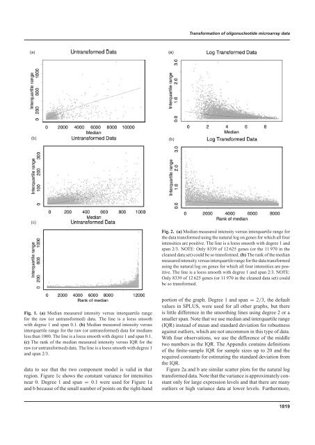
<strong>Transformation</strong> <strong>of</strong> <strong>oligonucleotide</strong> <strong>microarray</strong> <strong>data</strong>(a)(b)(b)(c)Fig. 2. (a) Median measured intensity versus interquartile range forthe <strong>data</strong> transformed using the natural log on genes for which all fourintensities are positive. The line is a loess smooth with degree 1 <strong>and</strong>span 2/3. NOTE: Only 8339 <strong>of</strong> 12 625 genes (or the 11 970 in thecleaned <strong>data</strong> set) could be so transformed. (b) The rank <strong>of</strong> the medianmeasured intensity versus interquartile range for the <strong>data</strong> transformedusing the natural log on genes for which all four intensities are positive.The line is a loess smooth with degree 1 <strong>and</strong> span 2/3. NOTE:Only 8339 <strong>of</strong> 12 625 genes (or 11 970 in the cleaned <strong>data</strong> set) couldbe so transformed.Fig. 1. (a) Median measured intensity versus interquartile rangefor the raw (or untransformed) <strong>data</strong>. The line is a loess smoothwith degree 1 <strong>and</strong> span 0.1. (b) Median measured intensity versusinterquartile range for the raw (or untransformed) <strong>data</strong> for mediansless than 1000. The line is a loess smooth with degree 1 <strong>and</strong> span 0.1.(c) The rank <strong>of</strong> the median measured intensity versus IQR for theraw (or untransformed) <strong>data</strong>. The line is a loess smooth with degree 1<strong>and</strong> span 2/3.<strong>data</strong> to see that the two component model is valid in thatregion. Figure 1c shows the constant variance for intensitiesnear 0. Degree 1 <strong>and</strong> span = 0.1 were used for Figure 1a<strong>and</strong> b because <strong>of</strong> the small number <strong>of</strong> points on the right-h<strong>and</strong>portion <strong>of</strong> the graph. Degree 1 <strong>and</strong> span = 2/3, the defaultvalues in SPLUS, were used for all other graphs, but thereis little difference in the smoothing lines using degree 2 or asmaller span. Note that we use median <strong>and</strong> interquartile range(IQR) instead <strong>of</strong> mean <strong>and</strong> st<strong>and</strong>ard deviation for robustnessagainst outliers, which are not uncommon in this type <strong>of</strong> <strong>data</strong>.With four observations, we use the difference <strong>of</strong> the middletwo numbers as the IQR. The Appendix contains definitions<strong>of</strong> the finite-sample IQR for sample sizes up to 20 <strong>and</strong> therequired constants for estimating the st<strong>and</strong>ard deviation fromthe IQR.Figure 2a <strong>and</strong> b are similar scatter plots for the natural logtransformed <strong>data</strong>. Note that the variance is approximately constantonly for large expression levels <strong>and</strong> that there are manyoutliers or high variance <strong>data</strong> at lower levels. Furthermore,1819