Transformation and normalization of oligonucleotide microarray data

More documents

Recommendations

Info

S.C.Geller et al.only 8339 of the 12 625 genes (or of the 11 970 genes of thedata subset) were usable as the other approximately 30% ofthe data had one or more of the replicates with non-positivevalues. Omission of such a large amount of data is not optimal.Even if it is considered that these data are unimportant in thissample, since the genes are not expressed at a high level, comparisonof different conditions is made much more difficult ifa gene is expressed at a low level in one sample and a highlevel in another. Simply replacing negative estimated expressionvalues by some arbitrary positive value such as 10 or 20,or by an estimated mean, is also non-optimal since it distortsthe variability pattern of the data.4 TRANSFORMATION AND NORMALIZATIONThe approach we pursue is to formulate a model that fits thevariance patterns in the data, and that contains normalizationconstants, and then use a procedure that can simultaneouslydetermine the transformation parameter and the normalization.The statistical model used is that, for gene i and chip j,the measured (average difference) value y ij satisfiesf c (y ij ) = µ i + n j + ɛ ij ,where µ i is the true expression of gene i in the sample, n j is anadditive chip normalization, and ɛ ij is an additive symmetricmeasurement error.The back-transformed, normalized measurementsỹ ij = fc−1 [f c (y ij ) − n j ]+αare assumed to fit the two-component model, so thatV(ỹ ij ) = σ 2 ɛ + S2 η µ2 i .In this model, Sη 2 = eσ η 2 (eση2 − 1), which is to the first orderthe same as ση 2. For example, if σ η = 0.1, corresponding to a10% coefficient of variation, then S η = 0.1008.The transformation used is[ √]f c (y) = ln y − α + (y − α) 2 + c ,where c = σɛ 2/S2 η , or equivalently to the first order c =σɛ 2/σ η 2 . Note that we could treat α as negligible given that theprimary data are PM–MM, which can be presumed to have amean near zero for unexpressed genes, but actually estimatedall the values, including α. We will briefly examine the resultof keeping α = 0. We can estimate σɛ2 from the low leveldata and ση 2 from the high level data, as in Rocke and Durbin(2001), but the values of σˆη , σˆɛ , and c are interdependent in thesense that we cannot determine σˆη and σˆɛ without knowing c,and vice versa. We solve this problem using the followingiteration:1. Starting with a trial value of c, transform the data using[ √]f c (y ij ) = ln y ij −ˆα + (y ij −ˆα) 2 + c .(We could use ˆα = 0 for these average difference dataor estimate it.)2. Determine the normalization constants n j by taking themedian of all genes over each slide minus the medianof all the genes on all the slides. Then, the transformed,normalized data aref c (y ij ) − n j .3. Back-transform the normalized transformed valuesusing the inverse transformationfc−1 (z) = ez − ce −z+ˆα.24. Determine the parameters σ ɛ and σ η of the twocomponentmodel by pooling low and high levels ofexpression as given in the Appendix and re-estimate α,a step not necessary when assuming that α = 0. We usea fixed number of genes at the high end, and at the lowend use all genes whose medians are sufficiently closeto α.5. Determine a new transformation parameter c = σɛ 2/σ η 2,and return to step 1 (using the original data not the backtransformeddata).6. Stop the process when the parameter values stopchanging.For this application, we did not assume that the averagedifference scores of unexpressed genes average out to nearzero, so that α is estimated, rather than assumed to bezero. We check out the effects of assuming α = 0 below.We estimated σ η by pooling IQRs of the log transformeddata corresponding to the highest h of the medians of the logtransformed data (see appendix). Also note that we cannotdetermine the transformation accurately without the iterativenormalization. In our data the flask effects (flask medianminus overall median) on the transformed scale ranged from1/4 to 3/4 of a robust estimate of the standard deviation of theerrors, so would have affected our computation of c.The above procedure was applied to the autism data. Itconverged after 25 iterations to c = 4300 (from σ ɛ =8.20 and σ η = 0.125 with α = 2.74 and h = 125).Figure [ 3 is a graph of the transformation, f 4300 (y) =ln y − 2.74 + √ ](y − 2.74) 2 + 4300 , over the range of thedata with a graph (dotted line) of z = ln [2(y − 2.74)], theequivalent log transform, for comparison. Figure 4a and b1820
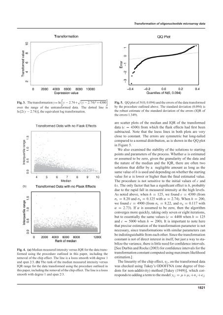
Transformation of oligonucleotide microarray data[Fig. 3. The transformation y= ln y − 2.74+ √ ](y − 2.74) 2 +4300over the range of the untransformed data. The dotted line isln [2(y − 2.74)], the equivalent log transformation.(b)Fig. 4. (a) Median measured intensity versus IQR for the data transformedusing the procedure outlined in this paper, including theremoval of the chip effect. The line is a loess smooth with degree 1and span 2/3. (b) The rank of the median measured intensity versusIQR range for the data transformed using the procedure outlined inthis paper, including the removal of the chip effect. The line is a loesssmooth with degree 1 and span 2/3.Fig. 5. QQ plot of N(0, 0.094) and the errors of the data transformedby the procedure outlined above. The standard deviation (0.094) isthe robust estimate of the standard deviation of the errors (IQR ofthe errors/1.349).are scatter plots of the median and IQR of the transformeddata (c = 4300) from which the flask effects had first beensubtracted. Note that the loess lines in both plots are veryclose to constant. The errors are symmetric but long-tailedcompared to a normal distribution, as is shown in the QQ plotin Figure 5.We also examined the stability of the solutions to startingpoints and parameters of the process. Whether α is estimatedor assumed to be zero, given the granularity of the data andthe nature of the median and the IQR, there are often twosolutions that differ by a negligible amount as long as thesame value of h is used and depending on whether the startingvalue for α is lower or higher than the final estimated value.The procedure is not sensitive to the initial values of c andks. The only factor that has a significant effect is h, probablydue to the rapid fall in measured intensity at the high levels.As noted above, when h = 125, we found c = 4300 (fromσ ɛ = 8.20 and σ η = 0.125 with α = 2.74). When h = 200,we found c = 4900 (from σ ɛ = 8.22, and σ η = 0.117 withα = 2.73). If α is assumed to be zero, then the algorithmconverges more quickly, taking only seven or eight iterations,but to essentially the same values (c = 4400 when h = 125and c = 5000 when h = 200). It is important to note herethat precise estimation of the transformation parameter is notnecessary, since transformations with similar parameters canbe indistinguishable from each other. Since the transformationconstant is not of direct interest in itself, but just a way to stabilizethe variance, there is little need for confidence intervals.[See Durbin and Rocke (2003) for confidence intervals for thetransformation constant computed using maximum likelihoodestimation.]The linearity of the chip effect, η j , on the transformed datawas checked using Tukey’s ODOFFNA (one degree of freedomfor non-additivity) method [Tukey (1949)], which correspondsto adding a term to the model y ij = µ+µ i +n j +e ij1821
Page 1 and 2: BIOINFORMATICSVol. 19 no. 14 2003,
Page 3: Transformation of oligonucleotide m
Page 7: Transformation of oligonucleotide m

Transformation and normalization of oligonucleotide microarray data

You also want an ePaper? Increase the reach of your titles

Delete template?

Save as template?