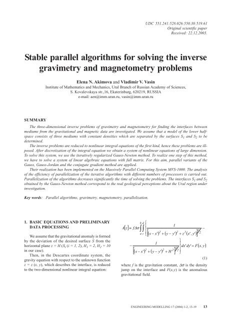
Stable parallel algorithms for solving the inverse gravimetry and ...

E.N. Akimova, V.V. Vasin: Stable parallel algorithms for solving the inverse gravimetry and magnetometry problemsThe magnetometry equation has the followingform:B[] z≡ ∆ J−b d∫∫⎧⎪⎨z( x' ,y' )22 2( x − x' ) + ( y − y' ) + z ( x' ,y' )[ ]3a c ⎪2⎩H22 2[( x − x' ) + ( y − y' ) + H ]32⎫⎪⎬dx'dy' = G⎪⎭−( x, y)(2)where G is the anomalous magnetic field and ∆J is theaveraged jump of the component z of the magnetizationvector.To select the anomalous gravity and magnetic field,which serve for the right-hand sides of Eqs. (1) and(2), we imply the following technique (see Ref. [1]).It is commonly accepted that the field recalculationupward to a level z=+H practically eliminates theeffect of anomaly-forming objects, located up to thedepth z=−H. By geological evidence, the field sourcesforeign to our analysis are located more deeply thanz=−H (H=2 km or H=10 km). Therefore, the measuredfield was continued upward to the level z=H.The stronger distortions in this procedure occurnear the boundary of the domain, hence the integrationis done over a finite area. To diminish these distortions,the values of a function that is the solution of the planeDirichlet problem were preliminary subtracted fromthe measured field. In the investigated domain thisfunction satisfies the two-dimensional Laplaceequation and coincides with the given field on theboundary of the domain.In our opinion, this function can be used as the fieldof the lateral sources. For recalculation upward, thePoisson formula for a subspace was used:U( x, y,H )≡12π+∞ +∞∫∫HU ( x' , y' ,0)2( x − x' ) + ( y − y' )dx' dy'2 2[ H ]−∞ − ∞+To get rid of the sources in the horizontal layer fromthe ground surface to the level z=−H, the fieldrecalculated upward was then continued downward tothe depth z=−H. In this case we solve the integralequation:1Kω≡2π= U+∞ +∞2Hω( x' , y' ) dx' dy'∫∫22−∞ −∞ ( x − x' ) + ( y − y' ) + ( 2H )( x, y,H )2[ ]to find the unknown function ω(x,y)=U(x,y,−H). Herethe function U(x,y,H) is given. In order to stably solvethis equation we used the Lavrentiev regularizationmethod of the form:(K+αI)ω = Ufor a suitable regularization parameter α>0.3232=Since the singularity of the function obtained liesbelow the plane z=−H, this function can be interpretedas the field of deep sources.The sum of this field recalculated on the groundsurface and the solution of the Dirichlet problem wasused as a field of lateral and deep sources (extrinsicsources). The difference of the measured field and thefield of the extrinsic sources was used as the gravityeffect (the function F(x,y) in Eq. (1)) of sources locatedin the horizontal layer from the ground surface to thedepth z=−H.The similar procedure was used for selecting theanomalous magnetic field (the function G(x,y) in Eq. (2)).2. ITERATIVE METHOD FOR SOLVINGTHE NONLINEAR SYSTEMAfter discretizing the Eqs. (1) and (2) on the gridn = M × N and approximating the integral operatorsA and B by the quadrature formulas, we obtain asystem of nonlinear equations of the form:A n[z] = F n(3)For solving this system the iteratively regularizedNewton method [2] is used:z k+1 = z k − [A' n(z k ) + α kI] -1 (A n(z k ) + α kz k − F n) (4)where A' n (z k ) is the Jacobi matrix calculated at thepoint z k , I is the identity operator, α k is a sequence ofthe positive parameters and F n is a vectorapproximation of the function F(x,y) (or G(x,y)).The iterative method of the Eq. (3) can be writtenin the following form:A k z k+1 = F k (5)where A k = A' n (z k ) + α k I is an n×n matrix, F k = A k z k −(A n (z k ) + α k z k − F) is an n-dimensional vector.So, for finding the next approximation z k+1 inNewton method, Eq. (4), it is necessary to solve thesystem of linear algebraic equations, Eq. (5), with fulln × n matrix.The careful analysis showed that, for aacceptable starting point z 0 and parameters α k , thematrix A k has n different eigenvalues for all realizediterations (k = 1,2,...,5).This implies that the corresponding eigenvectors arelinearly independent and the matrix S k whose columnsare eigenvectors has the inverse (S k ) -1 . Hence, the matrixA k can be represented in the form [3]:A k = S k Λ k (S k ) -1where Λ k is the diagonal matrix. From this formula itfollows that the matrix A k (k = 1, 2,..., 5) is invertible.Moreover, for problem described by Eq. (1) thecondition number cond(A k ) of the matrix A k varieswithin the intervals 2.8≤cond(A k )≤727 for the interfaceS 1 and 1.8≤cond(A k )≤2642 for the interface S 2 . Forproblem described by Eq. (2) the condition numbervaries within the intervals 1.1≤cond(A k )≤405 for theinterface S 1 and 1.2≤cond(A k )≤328 for the interface S 2 .14 ENGINEERING MODELLING 17 (2004) 1-2, 13-19

E.N. Akimova, V.V. Vasin: Stable parallel algorithms for solving the inverse gravimetry and magnetometry problemsThis guarantees the stability of calculations underthe realization of the iterative process given by Eq. (4)and the monotone decrease of the Newton methoderrors ∆ k =⏐z k − z⏐.The further analysis showed that, in fact, formethod given by Eq. (4) the conditions of the Newton-Kantorovich theorem [4] at the iteration points z k werefulfilled, which implies practical convergence of thismethod.It should be noted that if an operator A is monotone,then for any α k >0 the operator [A'(z)+α k I] -1 exists andis bounded, and under some conditions method givenby Eq. (4) converges to a solution of the equationA(z) = F for α k →0, k→∞ (see Ref. [2]). It is known[5] that the gravimetry operator is not monotone, sothe convergence theorem has not been proved.3. GAUSS, GAUSS-JORDAN ANDCONJUGATE GRADIENT METHODS.PARALLEL REALIZATIONSo, for finding the next approximation z k+1 for eachiteration of Newton method given by Eq. (4) it isnecessary to solve Eq. (5). The problem given by Eq. (5)can be solved by the Gauss or Gauss-Jordan eliminationalgorithms or by the conjugate gradient method.The main idea of the Gaussian elimination methodis reducing the full matrix A of system described byEq. (5) to the upper triangular form, that is, to obtainthe system of equations in the following form:⎧ x1+ c12x2+ c13x3+ ... + c1nxn= c1n+1⎪x2+ c23x3+ ... + c2nxn= c2n+1⎨⎪..............................................................⎪⎩xn= cnn+1(6)From system given by Eq. (6) we find theunknowns by the formulas:x k= c kn+1−c kk+1x k+1−...− c knx n, k=n, n-1,...,1 (7)The Gauss-Jordan algorithm is one of the variants ofthe Gaussian elimination algorithm. In this case the matrixA of system given by Eq. (5) is reduced to the diagonalform, but not an upper triangular form. In the (k+1)-thstep the current matrix A k has the following form:⎡( k) ( k)1 0 ... 0 a1,k 1... a ⎤⎢+1n ⎥⎢... ... ... ... ... ... ... ⎥⎢⎥⎢( k) ( k)0 0 ... 1 akk,k 1... a ⎥+knA = ⎢⎥ (8)⎢ ( k) ( k)⎥⎢0 0 ... 0 ak+ 1,k+ 1... ak+1,n ⎥⎢... ... ... ... ... ... ... ⎥⎢⎥⎢( k ) ( k0 0 ... 0 a)n,k+1... a ⎥⎣nn ⎦We divide the (k+1)-th row by the coefficienta (k) k+1 , k+1 and eliminate all off-diagonal elements ofthe (k+1)-th column. We make this elimination by thesubtraction of the obtained (k+1)-th row multiplied bya (k) j , k+l from the j-th row (j=1, 2,..., n; j≠k+1).To guarantee the numerical stability of the Gaussand Gauss-Jordan algorithms in the general case, apartial choice of the pivot element is necessary. If wetake the maximum (with respect to modulus) elementin the k-th row as the pivot element at the k-th step ofthe elimination, then, before realization of the step, itis necessary to rearrange the k-th column and thecolumn with the pivot element.The parallel realization of the Gauss or Gauss-Jordan method for m processors is the following.Conditionally, we divide the vectors z and F into mparts so that n=m⋅L. The matrix A is divided by thehorizontal lines into m blocks, respectively (Figure 1).¹¹¹¹ÀÓ×عÔÖÓ××ÓÖ½¹ÔÖÓ××ÓÖ¾¹ÔÖÓ××ÓÖºººÑ¹ÔÖÓ××ÓÖFig. 1 The diagram of the data distribution over the processorsAssume that the rows of the matrix A with numbers1, 2,..., L are stored in the memory of the first processor(the Host), the rows with numbers (L+1), (L+2),..., 2Lare stored in the memory of the second processor, andso on. The rows with numbers (m-1)L+1, ..., Lm arestored in the memory of the m-th processor. The mainidea of the parallel elimination is the following. At theevery step each processor eliminates the unknownsfrom its own part of the L equations. The Hostprocessor chooses the pivot element among theelements of the current row, modifies this row andsends it to each of the other processors [6].During the Gauss elimination process, more andmore processors become idle at every step, since thenumber of the equations is diminished by one. Thisinfluences the efficiency of the algorithm. In the Gauss-Jordan method all the processors make calculationswith their own parts until the end. The waiting timedecreases and the efficiency of the algorithm increases.The conjugate gradient method is used for solving theproblem with a symmetric matrix. For this we transformthe system given by Eq. (5) to the following form:(A k ) T A k z k+1 = (A k ) T F k (9)where (A k ) T is the conjugated matrix.For an arbitrary initial approximation z 0 , the firstapproximation z 1 is found from it by the steepestdescent method:020⋅ ( Az − F)0 0( Ar ,r )r1 00 0z = z −, r = Az − F (10)ENGINEERING MODELLING 17 (2004) 1-2, 13-19 15

E.N. Akimova, V.V. Vasin: Stable parallel algorithms for solving the inverse gravimetry and magnetometry problemsFurther from z 0 and z 1 we find all successiveapproximations of the conjugate gradient method:zk+1α =kβ =kk = 0,1,2,...k kk k−1z − αk( Az − F ) + βk( z − z )2k k k k k k kr ( Ap , p ) − ( r , p )( Ar , p ),k k k k k k 2( Ar ,r )( Ap , p ) − ( Ar , p )2k k k k k k kr ( Ar , p ) − ( r , p )( Ar ,r ),k k k k k k 2( Ar ,r )( Ap , p ) − ( Ar , p )=rpkk= Az= zkk− F− zk−1(11)The stopping condition of the iterative processgiven by Eqs. (10) and (11) is:Az k − FF< εParallelization of the iterative process given by Eqs.(10) and (11) for solving the problem given by Eq. (9)is based on the dividing of the matrices (A k ) T and A kby the horizontal lines into m blocks. The datadistribution over the processors is similar to the datadistribution in the Gauss method (Figure 1).At every step of the conjugate gradient method,each processor calculates its own part of the solutionvector z k . In the case of the multiplication of the matrixby the vector, each processor multiplies its own part ofrows of the matrix by the whole vector. In the case ofthe matrix product (A k ) T A k each processor multipliesits own part of rows of the conjugated matrix (A k ) T bythe whole matrix A k .4. EFFICIENCY OF THE METHODSParallelization of the basic algorithms and theirrealization on the Massively Parallel ComputingSystem MVS-1000 [7] is implemented. The analysisof the efficiency of parallelization of the iterativealgorithms with different numbers of processors iscarried out.MVS-1000/16 of the Research Institute KVANTproduction consists of 16 Intel Pentium III-800, 256MByte, 10 GByte disk, two 100 Mbit networkcontrollers (Digital DS21143 Tulip and Intel PRO/100). Educational computing cluster consists of 8 IntelPentium III700, 128 MByte, 14 GByte disk, 100 Mbitnetwork controller 3Com 3c905B Cyclone.For comparison of the executing times of thesequential and parallel algorithms, we will consider thecoefficients of the speed up and efficiency:S m= T 1/T m, E m= S m/mwhere T m is the execution time of the parallel algorithmon MVS-1000 with m (m>1) processors, T 1 is theexecution time of the sequential algorithm on oneprocessor:T m= T c+ T e+ T iwhere T c is the computing time, T e is the exchange timeand T i is the idle time. The number m of processorscorresponds to the mentioned division of the vectors zand F into m parts so that n=m⋅L.On the other hand, the efficiency can be calculatedusing only the parallel version of a program on aparallel computer without using the execution time ofthe sequential algorithm T 1 . The efficiency can bedefined as:E = G/(G + 1)where G is the granularity of a parallel algorithm [8].The granularity of a parallel algorithm is the ratioof the amount of computations to the amount ofcommunications within a parallel algorithmimplementation. Taking into account the possibilitythat the processors may be not equally balanced andthe processor idle time can occur, then the granularityis calculated using the following expression:G = T c/ (T e+ T i)The granularity may be estimated as:max TG ≤min( )comp⋅ m( T ) ⋅ mcommwhere max(T comp ) is the maximum computation timefor one processor and min(T comm ) is the minimumcommunication time for one processor.Table 1 and Table 2 show the execution times T mand the coefficients of the speed up S m and theefficiencies E m and E obtained by using the granularityG of the iteratively regularized Newton method after 5iterations using the parallel and sequential (m=1) Gaussand Gauss-Jordan algorithms for problems given by Eqs.(1) to (4) for 111×35 points of the grid domain.Table 1Table 2Gauss Method for the 111×35 gridm T m , min. S m E m E1 57.48 - - -2 46.85 1.23 0.61 0.663 36.18 1.59 0.53 0.594 29.38 1.96 0.49 0.565 25.78 2.23 0.45 0.536 21.83 2.63 0.44 0.528 17.25 3.33 0.42 0.4910 14.17 4.06 0.41 0.4812 12.35 4.65 0.39 0.44Gauss-Jordan Method for the 111×35 gridm T m , min. S m E m E1 114.1 - - -2 60.50 1.89 0.94 0.973 42.38 2.69 0.90 0.914 33.53 3.40 0.85 0.885 28.48 4.01 0.80 0.856 23.88 4.78 0.79 0.838 19.88 5.74 0.72 0.7810 16.45 6.93 0.69 0.7212 15.35 7.42 0.62 0.6616 ENGINEERING MODELLING 17 (2004) 1-2, 13-19

E.N. Akimova, V.V. Vasin: Stable parallel algorithms for solving the inverse gravimetry and magnetometry problemsTable 3Conjugate Gradient Method for the 111×35 gridm T m , min. S m E m E1 84.38 - - -2 43.20 1.95 0.98 0.994 22.75 3.71 0.93 0.955 18.63 4.52 0.90 0.9310 10.37 8.14 0.81 0.8411 9.67 8.79 0.80 0.8217 7.03 12.0 0.71 0.75Table 3 shows the execution times T m and thecoefficients of the speed up S m and the efficiencies E mand E obtained by using the granularity G of theiteratively regularized Newton method after 5iterations using the parallel and sequential (m=1)conjugate gradient method for problems given by Eqs.(1) to (4) for 111×35 points of the grid domain.The results of calculations show that the parallelGauss and Gauss-Jordan algorithms have efficiencyof parallelization high enough, and the Gauss-Jordanalgorithm efficiency is higher. But the conjugategradient method efficiency is higher than the efficiencyof the Gauss and Gauss-Jordan algorithms. This factcan be explained by the small exchange time. Theelements of the matrix (A k ) T A k are formedindependently in m processors. At every step of theconjugate gradient method, each processor calculatesits own part of the solution vector z k .In the case of the parallel Gauss algorithm with thenumber of processors m

E.N. Akimova, V.V. Vasin: Stable parallel algorithms for solving the inverse gravimetry and magnetometry problemsThey are reconstructed by the iteratively regularizedNewton method given by Eq. (4) with the help of theparallel Gauss or Gauss-Jordan algorithms or theconjugate gradient method.Fig. 8 The reconstructed interface S 2 forthe magnetometry problem6. CONCLUDING REMARKSFig. 5 The reconstructed interface S 1 forthe gravimetry problemThe main conclusion is the following. Theinterfaces S 1 and S 2 obtained as solutions of thegravimetry and magnetometry inverse problem, Eqs.(1) and (2), by the iteratively regularized Gauss-Newton method, Eq. (4), correspond to the realgeological perceptions about the investigated regionof the Urals.The nearest gravity and magnetic interfaces (seeFigure 3 and Figures 5 and 6) are rather different, butthe deeper interfaces (see Figure 4 and Figures 7 and8) are similar. We believe that, probably in the firstcase, the sources of the gravity and magnetic fields aredifferent, and in the second case these sources are thesame (or very close) and so we have the gravity andmagnetic solutions very close to each other.Fig. 6 The reconstructed interface S 1 forthe magnetometry problem7. ACKNOWLEDGEMENTSThe authors are deeply grateful to the RussianFoundation for Basic Research (project No. 03-01-00099) for the financial support.8. REFERENCESFig. 7 The reconstructed interface S 2 forthe gravimetry problem[1] V.V. Vasin, G.Ya. Perestoronina, I.L. Prutkin andL.Yu. Timerkhanova, Reconstruction of the reliefof geological boundaries in the three-layeredmedium using the gravitational and magneticdata, Proc. of the Conference on Geophysics andMathematics, Institute of Mines, UrB RAS,Perm, pp. 35-41, 2001.[2] A.B. Bakushinsky, A regularizing algorithm onthe basis of the Newton- Kantorovich method forthe solution of variational inequalities, Zh.Vychisl. Mat. Mat. Fiz., Vol. 16, No. 6, pp. 1397-1404, 1976.18 ENGINEERING MODELLING 17 (2004) 1-2, 13-19

E.N. Akimova, V.V. Vasin: Stable parallel algorithms for solving the inverse gravimetry and magnetometry problems[3] G. Streng, Linear Agebra and Its Applications,Mir, Moskva, 1980.[4] N.S. Bakhvalov, N.P. Zhidkov and G.M.Kobelkov, Numerical Methods, Nauka, Moskva,1987.[5] V.V. Vasin and A.L. Ageev, Ill-posed Problemswith a Priori Information, Nauka, Ekaterinburg,1993.[6] E.N. Akimova, Parallelization of an algorithm forsolving the gravity inverse problem, Journal ofComputational and Applied Mechanics, MiskolcUniversity Press, Vol. 4, No. 1, pp. 5-12, 2003.[7] A.V. Baranov, A.O. Latsis, C.V. Sazhin andM.Yu. Khramtsov, The MVS-1000 SystemUser’s Guide, http://parallel.ru/mvs/user.html.[8] J. Kwiatkowski, Evaluation of parallel programsby measurement of its granularity, Proc. of theConference on Parallel Processing and AppliedMathematics, Lecture Notes in ComputerScience, Vol. 2328, pp. 145-153, 2001.STABILNI PARALELNI ALGORITMI ZA RJE[AVANJE INVERZNIH GRAVIMETRIJSKIH IMAGNETOMETRIJSKIH PROBLEMASA@ETAKU ovom radu ispituju se trodimenzionalni inverzni problemi gravimetrije i magnetometrije da bi se prona{liodnosi izme|u medija pomo}u gravitacijskih i magnetskih podataka. Pretpostavljamo da model donjeg poluprostorasadr`i tri medija koji imaju stalne gusto}e, a odvojeni su pomo}u povr{ina S 1 i S 2 koje treba odrediti.Ovi inverzni problemi svedeni su na nelinearne integralne jednad`be prve vrste, prema tome ovi problemi sulo{e postavljeni. Nakon diskretizacije integralne jednad`be dobivamo sustav nelinearnih jednad`bi velike dimenzije.Koristimo iterativno reguliranu Gauss-Newton metodu da bi rije{ili ovaj problem. Moramo rije{iti sustav linearnihalgebarskih jednad`bi s punom matricom da bi realizirali jedan korak u ovoj metodi. Da se postigne ovaj cilj,primjenjuju se paralelne varijante Gaussove i Gauss-Jordan metode konjugiranog gradijenta.Njihova realizacija iskoristila se u Massively Parallel Computing System MVS-1000. Izvr{ena je analizaefikasnosti paralelizacije iterativnih algoritama pomo}u razli~itog broja procesora. Paralelizacija algoritamazna~ajno skra}uje vrijeme rje{avanja problema. Odnosi S 1 i S 2 koji su postignuti Gauss-Newton-ovom metodomodgovaraju stvarnoj geolo{koj predod`bi o podru~ju Urala koje se istra`uje.Klju~ne rije~i: Paralelni algoritmi, gravimetrija, magnetometrija, paralelizacija.ENGINEERING MODELLING 17 (2004) 1-2, 13-19 19