Stable parallel algorithms for solving the inverse gravimetry and ...

More documents

Recommendations

Info

E.N. Akimova, V.V. Vasin: Stable parallel algorithms for solving the inverse gravimetry and magnetometry problemsFurther from z 0 and z 1 we find all successiveapproximations of the conjugate gradient method:zk+1α =kβ =kk = 0,1,2,...k kk k−1z − αk( Az − F ) + βk( z − z )2k k k k k k kr ( Ap , p ) − ( r , p )( Ar , p ),k k k k k k 2( Ar ,r )( Ap , p ) − ( Ar , p )2k k k k k k kr ( Ar , p ) − ( r , p )( Ar ,r ),k k k k k k 2( Ar ,r )( Ap , p ) − ( Ar , p )=rpkk= Az= zkk− F− zk−1(11)The stopping condition of the iterative processgiven by Eqs. (10) and (11) is:Az k − FF< εParallelization of the iterative process given by Eqs.(10) and (11) for solving the problem given by Eq. (9)is based on the dividing of the matrices (A k ) T and A kby the horizontal lines into m blocks. The datadistribution over the processors is similar to the datadistribution in the Gauss method (Figure 1).At every step of the conjugate gradient method,each processor calculates its own part of the solutionvector z k . In the case of the multiplication of the matrixby the vector, each processor multiplies its own part ofrows of the matrix by the whole vector. In the case ofthe matrix product (A k ) T A k each processor multipliesits own part of rows of the conjugated matrix (A k ) T bythe whole matrix A k .4. EFFICIENCY OF THE METHODSParallelization of the basic algorithms and theirrealization on the Massively Parallel ComputingSystem MVS-1000 [7] is implemented. The analysisof the efficiency of parallelization of the iterativealgorithms with different numbers of processors iscarried out.MVS-1000/16 of the Research Institute KVANTproduction consists of 16 Intel Pentium III-800, 256MByte, 10 GByte disk, two 100 Mbit networkcontrollers (Digital DS21143 Tulip and Intel PRO/100). Educational computing cluster consists of 8 IntelPentium III700, 128 MByte, 14 GByte disk, 100 Mbitnetwork controller 3Com 3c905B Cyclone.For comparison of the executing times of thesequential and parallel algorithms, we will consider thecoefficients of the speed up and efficiency:S m= T 1/T m, E m= S m/mwhere T m is the execution time of the parallel algorithmon MVS-1000 with m (m>1) processors, T 1 is theexecution time of the sequential algorithm on oneprocessor:T m= T c+ T e+ T iwhere T c is the computing time, T e is the exchange timeand T i is the idle time. The number m of processorscorresponds to the mentioned division of the vectors zand F into m parts so that n=m⋅L.On the other hand, the efficiency can be calculatedusing only the parallel version of a program on aparallel computer without using the execution time ofthe sequential algorithm T 1 . The efficiency can bedefined as:E = G/(G + 1)where G is the granularity of a parallel algorithm [8].The granularity of a parallel algorithm is the ratioof the amount of computations to the amount ofcommunications within a parallel algorithmimplementation. Taking into account the possibilitythat the processors may be not equally balanced andthe processor idle time can occur, then the granularityis calculated using the following expression:G = T c/ (T e+ T i)The granularity may be estimated as:max TG ≤min( )comp⋅ m( T ) ⋅ mcommwhere max(T comp ) is the maximum computation timefor one processor and min(T comm ) is the minimumcommunication time for one processor.Table 1 and Table 2 show the execution times T mand the coefficients of the speed up S m and theefficiencies E m and E obtained by using the granularityG of the iteratively regularized Newton method after 5iterations using the parallel and sequential (m=1) Gaussand Gauss-Jordan algorithms for problems given by Eqs.(1) to (4) for 111×35 points of the grid domain.Table 1Table 2Gauss Method for the 111×35 gridm T m , min. S m E m E1 57.48 - - -2 46.85 1.23 0.61 0.663 36.18 1.59 0.53 0.594 29.38 1.96 0.49 0.565 25.78 2.23 0.45 0.536 21.83 2.63 0.44 0.528 17.25 3.33 0.42 0.4910 14.17 4.06 0.41 0.4812 12.35 4.65 0.39 0.44Gauss-Jordan Method for the 111×35 gridm T m , min. S m E m E1 114.1 - - -2 60.50 1.89 0.94 0.973 42.38 2.69 0.90 0.914 33.53 3.40 0.85 0.885 28.48 4.01 0.80 0.856 23.88 4.78 0.79 0.838 19.88 5.74 0.72 0.7810 16.45 6.93 0.69 0.7212 15.35 7.42 0.62 0.6616 ENGINEERING MODELLING 17 (2004) 1-2, 13-19
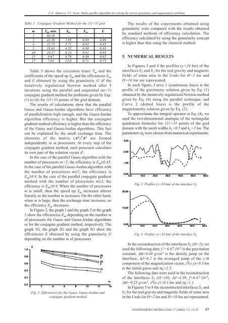
E.N. Akimova, V.V. Vasin: Stable parallel algorithms for solving the inverse gravimetry and magnetometry problemsTable 3Conjugate Gradient Method for the 111×35 gridm T m , min. S m E m E1 84.38 - - -2 43.20 1.95 0.98 0.994 22.75 3.71 0.93 0.955 18.63 4.52 0.90 0.9310 10.37 8.14 0.81 0.8411 9.67 8.79 0.80 0.8217 7.03 12.0 0.71 0.75Table 3 shows the execution times T m and thecoefficients of the speed up S m and the efficiencies E mand E obtained by using the granularity G of theiteratively regularized Newton method after 5iterations using the parallel and sequential (m=1)conjugate gradient method for problems given by Eqs.(1) to (4) for 111×35 points of the grid domain.The results of calculations show that the parallelGauss and Gauss-Jordan algorithms have efficiencyof parallelization high enough, and the Gauss-Jordanalgorithm efficiency is higher. But the conjugategradient method efficiency is higher than the efficiencyof the Gauss and Gauss-Jordan algorithms. This factcan be explained by the small exchange time. Theelements of the matrix (A k ) T A k are formedindependently in m processors. At every step of theconjugate gradient method, each processor calculatesits own part of the solution vector z k .In the case of the parallel Gauss algorithm with thenumber of processors m
Page 2 and 3: E.N. Akimova, V.V. Vasin: Stable pa
Page 6 and 7: E.N. Akimova, V.V. Vasin: Stable pa

Stable parallel algorithms for solving the inverse gravimetry and ...

You also want an ePaper? Increase the reach of your titles

Delete template?

Save as template?