Fundamentals of the Analog Computer - IEEE Xplore

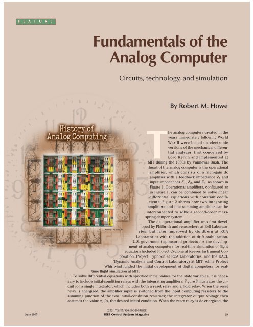
F E A T U R EFundamentals of theAnalog ComputerCircuits, technology, and simulationBy Robert M. HoweThe analog computers created in theyears immediately following WorldWar II were based on electronicversions of the mechanical differentialanalyzer, first conceived byLord Kelvin and implemented atMIT during the 1930s by Vannevar Bush. Theheart of the analog computer is the operationalamplifier, which consists of a high-gain dcamplifier with a feedback impedance Z f andinput impedances Z 1 , Z 2 , and Z 3 , as shown inFigure 1. Operational amplifiers, configured asin Figure 1, can be combined to solve lineardifferential equations with constant coefficients.Figure 2 shows how two integratingamplifiers and one summing amplifier can beinterconnected to solve a second-order massspring-dampersystem.The dc operational amplifier was first developedby Philbrick and researchers at Bell Laboratories,but later improved by Goldberg at RCA©DIGITALVISIONLaboratories with the addition of drift stabilization.U.S. government-sponsored projects for the developmentof analog computers for real-time simulation of flightequations included Project Cyclone at Reeves Instrument Corporation,Project Typhoon at RCA Laboratories, and the DACL(Dynamic Analysis and Control Laboratory) at MIT, while ProjectWhirlwind funded the initial development of digital computers for realtimeflight simulation at MIT.To solve differential equations with specified initial values for the state variables, it is necessaryto include initial-condition relays with the integrating amplifiers. Figure 3 illustrates the circuitfor a single integrator, which includes both a reset relay and a hold relay. When the resetrelay is energized, the amplifier input is switched from the input computing resistors to thesumming junction of the two initial-condition resistors; the integrator output voltage thenassumes the value e o (0), the desired initial condition. When the reset relay is de-energized, the0272-1708/05/$20.00©2005IEEEJune 2005 IEEE Control Systems Magazine29

amplifier input is reconnected to the input computingresistors, and the analog solution to the differential equationproceeds. Figure 3 also shows a hold relay that, whenInputVoltagesFigure 1. Operational amplifier. When the feedback and input impedances areresistors, the output voltage is proportional to the sum of the input voltages. Whena capacitor C is used as a feedback impedance, Z f = 1/(Cs) and the output voltageis proportional to the time integral of the sum of the input voltages.kf(t)− — dxdtf(t)− xme 1e 2e 3m/cmcm/kxZ 1 Zfi 1i fZ 2Z 3i 2i 3 e' dc AmplifierGain = −µe oLetting i 1 +i 2 +i 3 = i f and e' = − —1 e o , it follows from Ohm's Law thatµZFor the dc amplifier gain >> 1 + — f Z+ — f Zµ+ — f,Z 1 Z 2 Z 31Z f Z f Z— e fZ 1 + — e1 Z 2 + — e2 Z 33e o = ————————— .Z f Z f Z1+ 1 ⎡ — + — + — f ⎤µ –⎣1+ Z 1 Z 2 Z 3 ⎦Z f Z f Z fe o ≅ − ⎡— eZ 1 + — e1 Z 2 + — e2 Z 3⎤ .⎣3 ⎦m——d 2 x dx+ c — + kx = f(t), or ——d 2 x 1 c dx k= — f(t) − — — − —x .dt 2 dtdt 2 m m dt mResistors in megohms, capacitors in microfarads111x− dx23—dtFigure 2. Analog circuit for simulating a mass-spring-damper system. Amplifier 1 sumsthe terms in the equation for d 2 x/dt 2 and integrates the sum to obtain −dx/dt. Amplifier2 integrates −dx/dt to obtain x. Amplifier 3 simply inverts x to obtain −x. Note that allintegrators are inverting.11OutputVoltage− xenergized, disconnects the amplifier input from all inputresistors. This procedure then stops the integration andfreezes the integrator output voltage at its current value.The hold mode offers a useful methodfor accurately reading all integratorvalues at predetermined times duringan analog solution.To solve linear differential equationswith time-varying coefficients,the author utilized a stepping relay tovary the appropriate computing resistorof an operational amplifier at afixed sample rate in time. The resistorfor each time step was chosen so thatthe time integral of the resistor valuematched the time integral of the correspondingcontinuous time function.Figure 4 shows a simple example, ananalog circuit for solving Bessel’sequation of order zero.In [1], examples are given of analogsolutions of the time-dependenttransient responses of one- and twodegree-of-freedommechanical systems.The transient response ofsimple feedback control systems,where the analog computer solutionsare recorded as a function of the independentvariable time by using adirect-inking oscillograph, is exploredas well. Also shown are the solutionsof both Bessel’s and Legendre’sdifferential equations, which aresolved as second-order linearsystems with time-varying coefficientsusing the stepping-relayscheme described above (andshown in Figure 4) to approximatethe variable coefficients.Solutions for the static displacementof structural beams withvarious boundary conditionsand load distributions are alsosolved by allowing time on theanalog computer to correspondto distance along the beam. Thenormal-mode frequencies ofboth uniform and nonuniformbeams are solved as two-pointboundary-value problems, againby letting time on the analogcomputer represent distancealong the beam. Here the unknownratio of the two nonzero30 IEEE Control Systems MagazineJune 2005

initial state variables, together with the unknown eigenvaluefor each mode, are varied by trial and error until thetwo specified end conditions are met.Stability of Operational AmplifiersBecause the operational amplifier represents a feedbacksystem with a wide choice of feedback and input impedances,it is important to consider the dynamic requirementson the amplifier gain µ(s) to ensure closed-loopamplifier stability. These requirements can be understoodby breaking the feedback loop, as shown in Figure 5, withthe input impedance Z i grounded to represent zero inputvoltages. The overall open-loop transfer function is thengiven bye o(s) =−µZ i,e ′ Z i + Z falso known as the return ratio. For the closed-loop systemto be stable, the phase shift of the open-loop system mustbe more positive than −π at the frequency of unity openloopgain, defined as the crossover frequency. To be conservative,we usually require the phase shift of theopen-loop system to be equal to −π/2 at the crossoverfrequency. Clearly∣ |µ| =Z f + Z i ∣∣∣∣ Z iat the crossover frequency. If the feedback and inputimpedances are resistors, as in the case of a summingamplifier, then the crossover frequency occurs when|µ| = R f + R iR i.−e o (0)InputComputingResistors0.10.10.111 ResetRelayHoldRelayIntegratorOutputFigure 3. Circuit for integrator mode control. The resetrelay, when energized, establishes the initial condition forthe integrator. The hold relay, when energized, stops theintegration and freezes the output voltage e o .If the feedback impedance is a capacitor, then |Z f |≪|Z i |and the crossover frequency occurs when |µ| =1. Toensure that the open-loop phase shift is equal to −π/2 atthe crossover frequency for all possible summer and integratorconfigurations, it follows that the phase shift of theamplifier gain µ(s) should be −π/2 or greater at all frequenciesfor which |µ| > 1. When the dc operational amplifier isa stable minimum-phase system (no zeros or poles in theright-half plane), which is indeed the case for both vacuumtubeand transistor amplifiers, a phase shift of −π/2 orgreater is realized when the slope of the log |µ| versuslog |ω| plot is greater than or equal to −6 dB/octave. Figure5 shows the resulting open-loop frequency response.An example of a more complex configuration of feedbackand input impedances is the single amplifier circuit for simulatinga second-order linear system, as shown in Figure 6.To examine the stability of this feedback system, weground the input terminal −e i , break the feedback loop asshown in the figure, and let the open-loop input be e ′ o . Thisone-amplifier circuit for simulating a second-order systemcan be used in the feedback loop of a high-gain amplifier to0.11Ce o− — dxdt− xtˆ1——d 2 x 1 dx+ – — + x = 0, or ——d 2 x 1 dx= −– — −x .dt 2 t dtdt 2 t dt11111 23x− dx —dt11− x0.750.50.250tˆt0 0.25 0.5 0.75 1.0tFigure 4. Analog circuit for solving Bessel’s equation of order zero. The variable coefficient is approximated with the staircasefunction using a stepping relay.June 2005 IEEE Control Systems Magazine31

voltage cx, where c is acoefficient that can bee o '| µ (j ω)|set between 0 and 1. The(dB)diagram of the analogZ fcircuit for simulating thee'mass-spring-damper system,shown earlier in Fig-−µe oZ iZ f + Z iure 2, is repeated in6 dB/octFigure 7 using potentiometersto representReturn Ratio = — e Z ioe o 'the fixed coefficients in= Open-Loop Transfer Function 0log ωthe problem. The feedbackimpedances are notshown in the operationalFigure 5. Operational amplifier frequency response. This open-loop frequency response isamplifiers in Figure 7.needed to provide 90° of phase margin for any ratio of feedback to input impedances.Instead, only the fixedinput gains (nominally one or ten)are shown, with a triangle representinga summing amplifier and a1 d 2 e triangle attached to a vertical barDifferential equation: –— —— o 2ζde+ —– —— o+ e o = keω 2idt 2 n ω n dtrepresenting an integrating amplifier.Thus, in Figure 7, amplifiers 1R 3From Kirchhoff's and Ohm's Laws:and 2 are integrators, whereasC 2 e o ' amplifier 3 is an inverter. The inputRk = –— 3, ω1R 1RInput2n = —————— ,resistors m/c and m in Figure 2 areR 1 √ ⎯⎯⎯⎯ R 3 C 1 R 2 C 2 −e1e i oreplaced in Figure 7 with coefficientOutputω nC pots 1 and 2 set at c/m and 1/m,ζ = —– [R 12 + R 3 (1 + R 2 /R 1 )C 2 ]2respectively, in both cases drivingunity gain inputs. The input resistorm/k in Figure 2 is replaced byFigure 6. Single-amplifier circuit for simulating a second-order system when e o ′ = e o.For the closed-loop system to be stable with a phase margin of π/2, the open-loop frequencyresponse should exhibit a slope of −6 dB/octave at and around the frequency driving a gain-of-ten input. Pot 4 iscoefficient pot 4, set at 0.1 c/m andof unity (0 dB) open-loop gain.used in Figure 7 to set the initialcondition x(0) on the massobtain a representation of the reciprocal of a second-order displacement, whereas there is no indication of initialconditioncircuitry in Figure 2.system. The author utilized such a scheme to implementan electronic drive circuit for the two-channel direct-inking It should be noted that the setting of the output wiperoscillograph used for recording analog solutions. In this arm on the coefficient pot must take into account the inputcase, the recorder by itself was well represented by the resistor driven by the pot, since that input resistor is indynamics of a second-order system with an undamped naturalfrequency of approximately 30 Hz. When combined In general-purpose analog computers, the coefficient potsparallel with the pot resistance from wiper arm to ground.with the electronic drive circuitry described earlier, the are normally set in a pot-set mode, with the pot input xbandwidth of the overall recording system was extended replaced by +1 reference (that is, +100 V for analog computersbased on 100-V reference, and +10 V for analogto more than 100 Hz.computers based on 10-V reference). The pot is then set tothe desired value, either by reading a digital voltmeter orby means of a null meter connected between the pot outputand a reference pot with a precision dial. Note that thecoefficient pots are not set by reading the pot dials, eventhough the coefficient pots are usually ten-turn helical potswith precision, counter-type dials.It is apparent that the variables used in analog simulationsmust be properly scaled both to avoid over-rangingamplifier outputs and to ensure that amplifier outputsThe Use of Potentiometers to SetCoefficient Values in Analog SimulationsAll of the circuits described thus far for the analog solutionof differential equations have utilized resistors to setsumming and integrating amplifier gains. However, a muchmore practical method for implementing the precision settingof arbitrary coefficients in analog simulations utilizespotentiometers. For example, the potentiometer shown atthe top of Figure 7 with input voltage x provides an output32 IEEE Control Systems MagazineJune 2005

ange over a reasonable fraction offull-scale during any given solution.A similar problem occurs whenusing fixed-point digital computation.The simplest solution is torepresent each variable as a scaledfraction, the variable divided by itsmaximum value. Then each scaledfractionvariable will range over±1, which corresponds to ±100 Vin the case of 100-V analog computersand ±10 V in the case of 10-Vanalog computers. Actually, manyengineers (including the author)have found that the process ofscaling problem variables can lendconsiderable insight into the problemitself, including the identificationof dominant terms.Servomultipliers forAnalog ComputersAll of the example analog simulationsdescribed thus far haveinvolved the solution of linear differentialequations, including differentialequations with timevaryingcoefficients. Figure 8shows a schematic of a typical servomultiplier.The three gangedpotentiometers at the right side ofthe figure are driven by a twophaseinduction motor with an n:1gear reduction (not shown in thefigure). The servomotor is in turndriven by a magnetic amplifier,which receives its dc input from ananalog controller unit. The error inservo output angle is given byCoefficient Pote = X in − X out , where X in is the command input angle forthe servo and X out is the measured output angle, asobtained from the wiper arm output −X out of the potentiometerwith −100 V and +100 V connected to the highand low side, respectively. With ±Y and ±Z connectedacross the second and third potentiometers, the pot outputsrepresent XY and XZ, respectively. Note that the staticaccuracy of the servomultiplier depends on thelinearity of each ganged pot as well as the static nullingerror of the servo.Typical pots used in servomultipliers exhibit a maximumlinearity error ranging between 0.02% for ten-turnwire-wound, ganged potentiometers to 0.1% for one-turnganged potentiometers, either wire wound or film type.The static nulling error of the servomultiplier depends onxccxc/m1m——d 2 x+ c —dx+ kx = f(t), or 1/mdt 2 dt1 1 1f (t) 21 2xd 2 dxx 1 c dx k0.1k/mdt 2dtm m dt m1031Figure 7. Using potentiometers to set coefficient values in an analog simulation circuit.Note that pot 3 is set at 0.1 c/m because of the gain-of-10 input. To speed up thesetting of coefficients in large problems, servo-set potentiometers were widely used instate-of-the-art analog computers.X in11−X out1−eAnalogControllerCircuitFigure 8. A servomultiplier that uses a 60-Hz, two-phase servo motor driven by amagnetic amplifier. The analog controller circuit is used to provide additional damping.Typical multiplier accuracy was 0.1% or better. Because of the limited servobandwidth, the servo input X in should be assigned to the slower of the two variablesin computing a product.ux60-Hz Ref.MagneticAmplifierthe overall design of the servo, the static friction due toboth pot friction and gear-train friction, and the static resolutionof the ganged potentiometers. In the case of wirewoundpotentiometers, the static resolution is equal to thereciprocal of the number of wire turns, typically 3,000 forone-turn pots and more than 10,000 for ten-turn pots. Thestatic resolution error associated with conducting-filmpots can approach zero. To preserve static accuracy in theservomultiplier, it should also be noted that it is importantfor the multiplier pots with outputs XY and XZ in Figure 8to drive input resistors that are identical with the resistorthat loads the output −X out of the reference pot (that is, 1megohm in the example shown here).The transfer function of a typical servomotor plus themagnetic amplifier driver is given byc4–1(ref)–x(0)cx60-Hz Ref.ServoMotor−1003+Y+Z+100 −Y −ZXY XZ–xJune 2005 IEEE Control Systems Magazine33

M(s) =K m/ Is 2 + s/T m, (1)Input−eR fR C 1 1ZOutput u f= =K 1+ C es1−ue Z i τs + 1R 2Where K =R fC 2R 2, C e = (R 1 + R 2 ) C 1 , C i =1R 2 C 2,Figure 9. One-amplifier analog controller circuit for proportional, bandwidth-limitedrate and integral control. Alternatively, a circuit that requires two conventionalintegrating amplifiers and two summing amplifiers can be used.YXYXYX−100−100−1002R 1a2R 1aR 1b2R 2a2R 2aR 2b2R 3a2R 3aR 3b••••i 1D 3••••iFigure 10. Diode circuit for approximating ((X + Y)/2) 2 for X + Y > 0. The same circuitis repeated with inputs −X and −Y to approximate ((X + Y)/2) 2 for X + Y < 0. A similarpair of circuits with inputs X and −Y, and −X and Y, with diodes reversed and +100 biasvoltages, is used to approximate −((X − Y)/2) 2 . A single operational amplifier is used tosum the outputs of all four circuits to produce the product XY.where I is the total inertia of the servomultiplier(including servomotor, gear train, and ganged potentiometersreferred to the servo output shaft) and T m isthe motor time constant. If the analog controller circuitin Figure 8 consists of a pure gain K , then the overallservo transfer function is approximately represented bya second-order system with an undamped natural frequencygiven by ω n = √ KK m / I and damping ratio givenby ζ = (1/2) √ I/KK m /T m . To obtain satisfactory nullingerrors, the gain constant K for typical servomultipliersmust be sufficiently large that the resulting damping ratioζ is too small for satisfactory transient performance. Thus,it is necessary to add rate control to the proportional controlin the analog controller circuit. It also may be desirableto add integral control to ensure low nulling error(that is, good servo tracking) for a slowly varying input X in .Figure 9 shows an operational amplifier circuit that providesthe necessary controller transfer function, where therate control term C e s is bandwidthlimitedby the transfer function1/(τs + 1).The overall servomultiplier transferfunction for sinusoidal inputsτ = R 1 C 1 .(1+ C i s −1 )X+Y X+Yi=i 1 ...X+Yi 2D 1+i 2 +i 3 +2D 2 i 2X+Yi 3i 1≡ −X+Yi 30.1predicts the dynamic performanceof the closed-loop system based onlinear models of the subsystems.However, the servomotor has twoimportant characteristics that arenot modeled by the motor transferfunction (1). These characteristicsinclude the acceleration limit|X ′′ | max and the velocity limit |X ′ | maxfor large motor controlinputs. The experiencegained in designing servomultipliersfor analog computersled to the realizationthat the design of an electromechanicalcontrol system,2including the choice of components,is dominated bynonlinear requirements suchas the acceleration andvelocity limits (large-motionnonlinearities) and thenulling error or static resolution(small-motion nonlinearities).The role of lineardesign methods is generallylimited to the choice of controllerparameters needed toproduce satisfactory systemstability margin and transientresponse [2].Other NonlinearAnalog-ComputerComponentsWhile the servomultipliersdescribed above were widelyutilized in analog computers34 IEEE Control Systems MagazineJune 2005

during the 1950s, several alternative, all-electronic deviceswere developed to improve the overall dynamics of analogmultipliers. The first of these was the time-division multiplier,initially developed by Goldberg [3]. In this scheme,the voltage X is converted to a pulse-width modulated signalused to drive an electronic switch, which modulatesthe voltage Y. The area under each cycle of the switchedsignal is proportional to the product XY. The switched signaldrives a low-pass filter to produce a smoothed outputXY. Although time-division multipliers achieved dynamicerrors that were typically two orders of magnitude smallerthan those associated with servomultipliers, these multipliersoften exhibited undesirable drift in voltage offsetwith time. Another device was the quarter-square multiplier,which was based on the equationXY = (X + Y)2 − (X − Y) 2. (2)4The circuit shown in Figure 10 is used to generate a segmentedapproximation to ((X + Y)/2) 2 for X + Y > 0.When X + Y becomes positive enough, the diode D 1 startsconducting and the current i 1starts to increase linearly forfurther increases in X + Y. For alarger value of X + Y, diode D 2starts to conduct, and the currenti 2 starts to increase linearlywith increasing X + Y . Theoverall circuit in Figure 10 consistsof n diode segments. Theamplifier output in Figure 10then produces an n-segmentapproximation to −((X + Y)/2) 2for X + Y > 0. With idealdiodes, the segmented approximationto a quadratic functionthen exhibits a maximum fractionalerror of 1/(8n 2 ). With thesilicon-junction diodes normallyused for quarter-square multipliers,the nonideal diode current-voltagecharacteristicproduces additional rounding ofeach segment knee, furtherreducing the quadratic-approximationerror.It should be noted that (2) forthe quarter-square multiplier canbe replaced with the formulaXY = |X + Y|2 −|X − Y| 2.4XY−X−YX−Y−XYRRRRRRRRDa1By replacing (X + Y) 2 with |X + Y| 2 and replacing (X − Y) 2with |X − Y| 2 , we can eliminate the need for two of the foursegmented quadratic approximation circuits similar to theone shown in Figure 10. Furthermore, the calculation of|X + Y| and |X − Y| can be combined with the diode circuitfor the segmented quadratic approximation by using the circuitshown in Figure 11. Here the voltage at the junction ofdiodes D a1 and D a2 is proportional to |X + Y|/2, and thevoltage at the junction of diodes D a3 and D a4 is proportionalto −|X − Y|/2, as indicated in Figure 11. These diode-junctionvoltages then drive biased-diode circuits similar to theone in Figure 10 to produce segmented approximations tothe quadratic function. Because of the loading effect of thebiased-diode circuits on the passive absolute-value circuit inFigure 11, the effect of the nonideal diode characteristics onthe rounding of the knees of the segmented approximation isincreased. This rounding in turn causes error in the segmentedapproximation to the quadratic function to be considerablyless than the value of 1/(8n 2 ) for ideal diodes, where nis the number of diode segments used for the quadraticapproximation. Thus, the completely passive quarter-squaremultiplier circuit of Figure 11, in addition to reducing by∝ X−Y2R 1b−V b1D a2 R 2aR 2b−V b1D 2• •• •∝− X−Y2• •• •R 1aR 1b+V b1R 2aR 2bFigure 11. A completely passive quarter-square multiplier circuit terminated in a singleoperational amplifier. The circuit is based on XY = (|X + Y|/2) 2 − (|X − Y|/2) 2 . Thecircuit output is connected to the summing junction of an operational amplifier with a0.1 m feedback resistor.R 1a••••••••0.1≡XYJune 2005 IEEE Control Systems Magazine35

more than a factor of two the number of required components,also is more accurate than the circuit in Figure 10 for agiven number n of diode segments. The author developed aten-segment version of this circuit in 1959.It should be noted that analog division of Y by X can beaccomplished by utilizing a multiplier in the feedback loopof an operational amplifier. With the amplifier input connectedto −Y, the multiplier input X in connected to X , themultiplier input Y in connected to the amplifier output, andthe multiplier output X in Y in connected to the amplifierfeedback resistor, the amplifier output is the quotient Y/X .The generation of a function f(X ) can be accomplished inanalog computation by using a segmented approximation tof(X ). The segmented approximation can be generated usinga diode function generator, which consists of biased-diodecircuitry similar to that shown in Figure 10, with potentiometersused to set the slope and breakpoint of each diode segment.Alternatively, a servomultiplier can be used, with ntaps on one of the servo-driven pots. Padding resistors connectedbetween the taps can then be adjusted to obtain thepot output Yf(X ), with f(X ) represented by an approximationwith n + 1 straight-line segments. Similarly, the functionssin(X ) and cos(X ) are generated either by diodefunction generators or servo-driven sine-cosine pots. For adescription of these and other analog components, see [4].One of the first implementations of time-optimal control wasaccomplished using biased-diode analog circuitry to representthe required nonlinear control law [5]. Also, the outputsaturation voltage characteristics of unstabilized operationalamplifiers were used to represent simple nonlinearities, suchas relay-type bang-bang controllers and Coulomb friction [6].Current Availabilityof Analog ComponentsIt should be noted that many of the components utilized inthe early analog computers are currently available in integrated-circuitform. For example, operational amplifierswith bandwidths and drift characteristics equal to or betterthan the drift-stabilized amplifiers of two or threedecades ago are available at a fraction of the cost, with upto four amplifiers located on a single chip. Nevertheless,with the current and projected speed of digital-processorchips, it seems unlikely that analog computers will everagain match their prominent former role as a general-purposedevice for the simulation of dynamic systems.References[1] D.W. Hagelbarger, C.E. Howe, and R.M. Howe, “Investigation of theutility of an electronic analog computer in engineering problems,Aeronautical Research Center, Engineering Research Institute,Univ. Michigan, Ann Arbor, Michigan, UMM-28, Apr. 1, 1949.[2] E.O. Gilbert, “The design of position and velocity servos for multiplyingand function generation,’’ IRE Trans. Electron. Comput., vol. EC-8,no. 3, pp. 391–399, Sept. 1959.[3] E.A. Goldberg, “A high-accuracy time-division multiplier,’’ RCA Rev.,vol. 13, no. 3, pp. 265–274, Sept. 1952.[4] R.M. Howe, Design Fundamentals of Analog Computer Components.Princeton, NJ: D. van Nostrand, 1961.[5] R.M. Howe and L.L. Rauch, “Physical implementation of a torquesaturatedlinear servo with optimum step response,’” in Proc. JointAutomatic Control Conf., Cambridge, Mass. Sept. 1960.[6] R.M. Howe, “Representation of nonlinear functions by means ofoperational amplifiers,’’ I.R.E. Trans. Electron. Comput., vol. EC-5, pp.203–206, Dec. 1956.Robert M. Howe, one of the founders of Applied DynamicsInternational (ADI) and Professor Emeritus at the University ofMichigan, where he taught for 41 years. This image showsone of the latest ADI products, a distributed rtX system utilizingmultiple PCs for real-time hardware-in-the-loop simulation.Robert M. Howe (bobhowe@umich.edu) is Professor Emeritusof Aerospace Engineering at the University of Michigan,where he served on the faculty for 41 years, including 15years as department chair. He received a B.S. in electricalengineering from Caltech. He received an A.B. from OberlinCollege, an M.S. from the University of Michigan, and a Ph.D.from MIT, all in physics. His interests include real-time simulation,as well as flight dynamics and control. He is the authorof over 100 technical papers and one book on analog computers.He served as the first national chair of Simulation Councils,Inc., the predecessor of the Society for ComputerSimulation. His many honors include the 1983 AIAA de FlorezTraining Award for Flight Simulation and the 1978 Award forMeritorious Civilian Service for “outstanding contributions inguidance and control, and flight simulation” while a memberof the USAF Scientific Advisory Board. He has served as atechnical consultant to many companies. His technical societymemberships include AIAA (Associate Fellow), SCS, andIEEE (Fellow). He was a founder of Applied Dynamics International,an Ann Arbor computer company for which he continuesto consult since his retirement in 1991 from theUniversity of Michigan. He can be contacted at 485 RockCreek Dr., Ann Arbor, MI 48104 USA.36 IEEE Control Systems MagazineJune 2005