Chapter I: Review of important results in quantum Mechanics - LSU

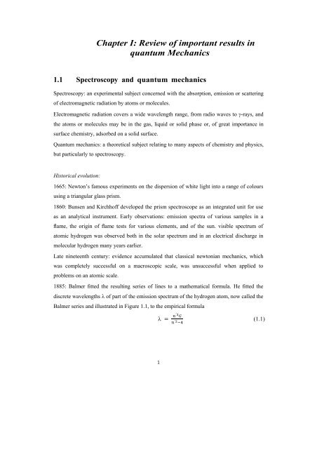
Chapter I: Review of important results inquantum Mechanics1.1 Spectroscopy and quantum mechanicsSpectroscopy: an experimental subject concerned with the absorption, emission or scatteringof electromagnetic radiation by atoms or molecules.Electromagnetic radiation covers a wide wavelength range, from radio waves to -rays, andthe atoms or molecules may be in the gas, liquid or solid phase or, of great importance insurface chemistry, adsorbed on a solid surface.Quantum mechanics: a theoretical subject relating to many aspects of chemistry and physics,but particularly to spectroscopy.Historical evolution:1665: Newton’s famous experiments on the dispersion of white light into a range of coloursusing a triangular glass prism.1860: Bunsen and Kirchhoff developed the prism spectroscope as an integrated unit for useas an analytical instrument. Early observations: emission spectra of various samples in aflame, the origin of flame tests for various elements, and of the sun. visible spectrum ofatomic hydrogen was observed both in the solar spectrum and in an electrical discharge inmolecular hydrogen many years earlier.Late nineteenth century: evidence accumulated that classical newtonian mechanics, whichwas completely successful on a macroscopic scale, was unsuccessful when applied toproblems on an atomic scale.1885: Balmer fitted the resulting series of lines to a mathematical formula. He fitted thediscrete wavelengths of part of the emission spectrum of the hydrogen atom, now called theBalmer series and illustrated in Figure 1.1, to the empirical formula (1.1)1

where is a constant and In this figure, the wavenumber and thewavelength are used and are related by (in cm-1 ) (1.2)Using the relationship (in sec-1 ) (1.3)where is the frequency and the speed of light in a vacuum, Equation (1.1) becomes (1.4) in which is the Rydberg constant for hydrogen. The discrete rather than continuous natureof the spectrum is completely at variance with classical mechanics.1887: Hertz observes that when ultraviolet light falls on an alkali metal surface, electrons areejected from the surface only when the frequency of the radiation reaches a thresholdfrequency , which depends on the metal. As incident frequency increases, the kinetic energyof the ejected electrons (known as photoelectrons) increases linearly with (Figure 1.2).Photoelectric effect was unexplained by classical physics.Explanation of spectrum of hydrogen atom and of the photoelectric effect, together with otheranomalous observations such as the behaviour of the molar heat capacity of a solid attemperatures close to and the frequency distribution of black body radiation, originatedwith Planck.1900: Planck proposed that microscopic oscillators, of which a black body is made up, havean oscillation frequency related to the energy of the emitted radiation by (1.5)where is an integer; is known as the Planck constant and its presently accepted value is (1.6)The energy is said to be quantized in discrete packets, or quanta, each of energy .Because is very small (it can be considered the energy etalon of the microscopic world),quantization of energy in macroscopic systems had escaped notice.2

1906: Einstein applied this theory to the photoelectric effect and showed that (1.7)where = energy associated with a quantum (Lewis called it a photon in 1924) of theincident radiation, = kinetic energy of the photoelectron ejected with velocity : =ionization energy of the metal surface (also called the work function for solids).1913: Bohr combined classical and quantum mechanics to explain observation of the Balmerseries but also of the Lyman, Paschen, Brackett, Pfund, etc., series of the hydrogen atomemission spectrum (Figure 1.1). He assumed empirically that the electron can move only inspecific circular orbits around the nucleus and that the angular momentum for an angle ofrotation is given by where and defines the particular orbit. Energy is emitted or absorbed when theelectron moves from an orbit with higher to one of lower , or vice versa. The energy of the electron (derived by classical mechanics) is:(1.8) (1.9)where = is the reduced mass of the system of electron e and proton p;e = electronic charge; = permittivity of a vacuum. E n ‘s are the energy levels in Figure 1.1but = is plotted. Zero of energy corresponds to , i.e. atom is ionized. Energylevels discrete below but continuous above, since electron can be ejected with anyamount of kinetic energy.When the electron transfers from, say, a lower to an upper orbit, energy requiredis (from equation (1.9)) or, since (1.10) (1.11)from comparison with Equ. (1.4): and for the Balmer series.3

Similarly: , and 5 for Lyman, Paschen, Brackett and Pfund series, …However, it is important to realize that there is an infinite number of series, e.g. series withhigh are observed in the interstellar medium (rich in H) by radioastronomy. For example,the transition at .The Rydberg constant from Equ. (1.11) is: (1.12)Planck’s quantum theory: very successful in explaining the hydrogen atom spectrum, thewavelength distribution of black body radiation, the photoelectric effect and the low-temperature heat capacities of solids, but also gave rise to apparent anomalies: in thephotoelectric effect, photons are particles, while in interference and diffraction, light is awave.1924: de Broglie proposes the wave-particle duality: (1.13)momentum (a particle property) is related to the wavelength (a wave property).1925: Davisson and Germer showed that electron can be wave-like by their diffraction atsurface of crystalline nickel. Their experiment formed the basis of the LEED (low-energyelectron diffraction) technique for investigating structure near the surface of crystallinematerials.1930: Further confirmation by Mark and Wierl showed that transmission of an electron beamthrough a gas target resulted in diffraction.Wave-particle duality rationalises why electron in H atom may be only in particular orbitswith angular momentum given by Equation (1.8). In wave picture, circumference of anorbit of radius r must contain an integral number of wavelengths (1.14)where , 1, for a standing wave to be set up (see Figure 1.3(a) for , and4

Figure 1.3(b) shows how a travelling wave results when is not an integer: the waveinterferes with itself and is destroyed).However, electron in an orbit as a standing wave poses the important question of where theelectron, regarded as a particle, is. We shall consider the answer to this for the case of anelectron travelling with constant velocity in a direction . The de Broglie picture of this is ofa wave with a specific wavelength travelling in direction as in Figure 1.4(a), and it is clearthat we cannot specify where the electron is. At the other extreme we can consider theelectron as a particle which can be observed as a scintillation on a phosphorescent screen.Figure 1.4(b) shows how, if there is a large number of waves of different wavelengths andamplitudes travelling in the direction, they may reinforce each other at a particular value of, say, and cancel each other elsewhere. This superposition at is called a wave packetand we can say the electron is behaving as if it were a particle at .For Figure 1.4(a), momentum of electron is defined its position is completely uncertain.In Figure 1.4(b), is certain but the wavelength, and therefore , is uncertain.1927: Heisenberg’s uncertainty principle: (1.15)With h / 2. In extreme wave picture, and , in extreme particlepicture, and . Other important form of the uncertainty principle: (1.16)(time , energy ), i.e. if energy of a state known exactly, and . Such a statedoes not change with time and is known as a stationary state.1.3 The Schrödinger equation and some of its solutionsMany references given on QM in the bibliography, end of this chapter. Here, we briefly recallthe development of the Schrödinger equation and some of its solutions that are vital to theinterpretation of atomic and molecular spectra.5

1.3.1 The Schrödinger EquationJust as travelling light wave can be represented by a function of its amplitude at a particularposition and time, so it was proposed that a wave function , a function of position andtime, describes the amplitude of an electron wave.1926: Born relates the wave and particle views by saying that we should speak not of a particlebeing at a particular point at a particular time but of the probability of finding the particle there.This probability is , where is the complex conjugate of (obtained by replacing all in by . It follows that:=. Reasonable also that: (1.17) (1.18)1928: Dirac shows that, when relativity is taken into account, this is not quite true, but we shall notbe concerned with the effects of relativity.The form postulated for the wave function is (1.19)where is a constant and is the action, which is related to the kinetic energy and the potentialenergy by (1.20) the sum of the kinetic and potential energies (i.e. same as the hamiltonian in classicalmechanics). From Equations (1.19) and (1.20): (1.21)The form of the hamiltonian in quantum mechanics is obtained by replacing the kinetic energy inEquation (1.20), giving (1.22)6

(Symbol , called ‘del’), in cartesian coordinates , known as the laplacian, is: (1.23)From Equ. (1.21) and (1.22), time-dependent Schrödinger equation: In conventional (frequency domain) spectroscopy, time-independent part is mainly of concern.Consider (for ease of manipulation), wave travelling in the direction, and assume that: can be factorized into a giving (1.25)Where time-dependent part and time-independent part . Combination of Equ. (1.24), fora one-dimensional system, and Equ. (1.25) gives 7 (1.26)Since the left-hand side (LHS) is function of x only, and the right-hand side (RHS) function of tonly, they must both be constant. Since they have the same dimensions as (i.e. energy) weput them equal to . For LHS: (1.27) one-dimensional time-independent Schrödinger equation (also called the wave equation): (1.28)with H= hamiltonian (equ. 1.22, but for one dimension only). contains , i.e. it is an operator(e.g., is an operator which operates on to give ). In Equ. (1.28) operating on by givesthe result of multiplied by an energy . For example: (1.29)We are concerned with stationary states, known sometimes as eigenstates. The wave functions forthese states may be referred to as eigenfunctions and the associated energies as the eigenvalues.See bibliography for methods of solving the Schrödinger equation for and for various systems.Here are some systems of interest here.

1.3.2 The hydrogen atomThe H atom (a proton and one electron), occupies a very important position in the development ofquantum mechanics because the Schrödinger equation may be solved exactly for this system. Alsotrue for hydrogen-like atomic ions , , , etc., and simple one-electron molecular ionssuch as .In QM picture of H atom, total energy is quantized and has exactly the same values as in Equ.(1.9). Angular momentum of the electron in a particular orbit (also called orbital) may also takeonly discrete value, is a vector and is defined, therefore, by its magnitude and direction. In theclassical picture of an electron circulating in an orbit in the direction shown in Figure 1.5 thedirection of the corresponding vector, which is also shown, is given by the right-hand screw rule.In a magnetic field, can take only certain orientations with respect to the magnetic field direction,so that the component of in that direction can take only certain, discrete values. Thisphenomenon is referred to as space quantization. The effect is known as the Zeeman effect.For the hydrogen atom: (1.30)Second term on RHS is coulombic potential energy for the attraction between charges and a distance apart. Laplacian is here defined in spherical coordinates as: (1.31)= distance of a point from the origin; = co-latitude; = azimuth (Figure 1.6). The wavefunctions corresponding to the hamiltonian of Equation (1.30) may be factorized: (1.32) are angular wave functions. They describe distribution of over the surface of a sphere ofradius , i.e. they are spherical harmonics. Quantum number is same as in Bohrtheory, is the azimuthal quantum number associated with the discrete orbital angular momentumvalues, and is known as the magnetic quantum number which results from the spacequantization of the orbital angular momentum:(1.33) (1.34)8

in Equation (1.32) can be factorized further to give (1.35)The functions are the associated Legendre polynomials (table 1.1), and are independent of .They are therefore the same for all one-electron atoms.The solution of Schrödinger equation for radial wave functions (they are functions only of), follows a well-known mathematical procedure to produce the solutions known as the associatedLaguerre functions, of which a few are given in Table 1.2. The radius of the Bohr orbit for isgiven by (1.36)For hydrogen, , and a useful quantity is related to by (1.37)Orbitals are labelled according to values of and . The symbols s, p, d, f, g, ... indicate values of . Thus we speak of 1s, 2s, 2p, 3s, 3p, 3d, etc. orbitals where the 1, 2, 3, etc. referto the value of .There are three useful ways of representing graphically:1. vs (or ), Figure 1.7(a). It can be seen that and are always positive but changes from positive to negative and, at one value of , is zero.2. vs (or ), Figure 1.7(b). = probability of finding electron between and, i.e. this plot represents the radial probability distribution of the electron.3. vs (or ), Figure 1.7(c). = radial charge density, and is the probabilityof finding the electron in a volume element consisting of a thin spherical shell of thickness, radius , and volume .Diagrammatic representations of the functions (Equ. 1.35) cannot be made unless weconvert them from imaginary into real functions (Except when ).In the absence of an electric or magnetic field all the functions with are folddegenerate ( functions with the same energy, and each a possible values of .A property of degenerate functions: linear combinations of them are also solutions of theSchrödinger equation. e.g., just as and are solutions of the Sch. Eq., so are9

- (1.38) From Equations (1.32), (1.35) and (1.38), together with the functions in Table 1.1, itfollows thatsince (1.39) (1.40)Equs (1.39) become (1.41) (1.42)In addition, the third degenerate wave function is always real, and we label it ,where (1.43)All wave functions are always real and so are the , , etc. wave functions for However, for with , it is necessary to form linear combinations of theimaginary wave functions and , or and , to obtain real functions. The orbital wave functions for any are distinguished by subscripts , and , and and . There are seven orbitals for any but we shall not consider them here.Figure 1.8 shows the real wave functions for the 1s, 2p and 3d orbitals in the form ofpolar diagrams. For the case of the orbital, the wave function (equ. 1.43) is independent of and proportional to . The polar diagram consists of points on a surface obtained by markingoff, on lines drawn outwards from the nucleus in all directions, distances proportional to at a constant value of . The resulting surface consists of two touching spheres (Figure 1.8,10

also shows polar diagrams for all 1s, 2p and 3d orbitals). Figure 1.7 shows that as .Polar diagrams are drawn as surface boundaries within which approx. 90% of the wavefunction resides.For all orbitals (except 1s) there are regions in space where because, and/or . Electron density is zero and we call them nodal surfaces or nodes. For example,the orbital has a nodal plane, while each of the 3d orbitals has two nodal planes. In general,there are such angular nodes where . The 2s orbital has one spherical nodal plane, orradial node, as Figure 1.7 shows. Generally, there are radial nodes for an orbital (or if we count the one at infinity).Quantum mechanical solution: same as in the Bohr theory (Equation (1.9)), it must do sincethe Bohr theory agrees exactly with experiment, except for the fine structure of the spectrum,which our present quantum mechanical treatment has not explained either. The probabilitydistributions of figs 1.7 and 1.8, contain function assymptotically going to zero and nodalsurfaces with zero probability of finding the electron. This is far from the classical picture of theelectron orbiting round the nucleus like the moon orbiting round the earth.Unlike the total energy, the quantum mechanical value of the orbital angular momentum issignificantly different from that in the Bohr theory given (equ. 1.8). It is now given by (1.44)where .An effect of space quantization of orbital angular momentum may be observed if a magneticfield is introduced along the axis. The orbital angular momentum vector , of magnitude ,may take up only certain orientations such that the component along the axis is given by (1.45)where . This is illustrated in Figure 1.9 for an electron in a orbital .1.3.3 Electron spin and nuclear spin angular momentumThe electron and the nucleus can each spin on its own axis, and each has an angular momentumassociated with spinning. This is the origin of the electron spin and the nuclear spin.Quantum mechanical treatment: magnitude of the angular momentum due to the ‘spin’ of oneelectron is11

(1.46)where s =only. This result cannot be derived from the Schrödinger equation but only fromDirac’s relativistic quantum mechanics. Space quantization of this angular momentum results inthe componentwhere only (Figure 1.10). (1.47)Similarly, the magnitude of the angular momentum due to nuclear spin is given by (1.48)The nuclear spin quantum number may be zero, half-integer or integer, depending on the nucleusconcerned. Nuclei contain protons and neutrons, each with . The way in which the spinangular momenta of these particles couple together determines the value of , a few being given inTable 1.3. It is essential for nuclear magnetic resonance spectroscopy that for the nucleibeing studied, so that, for example,nuclei cannot be used.1.3.4 The Born–Oppenheimer approximationHamiltonian H (eq. 1.20): In molecule, kinetic energy T consists of contributions T e and T n fromthe motions of the electrons and nuclei, respectively. Potential energy comprises two repulsiveterms, and (electron-electron and nucleus-nucleus interactions), and , due to attractiveinteractions between the electrons and nuclei, giving (1.49)For fixed nuclei , and , and there is a set of electronic wave functions which satisfy the Schrödinger equation (1.50)where (1.51)Since depends on nuclear coordinates, because of the term, so do and .1927: Born–Oppenheimer approximation: assumes nuclei move so slowly compared with electronsthat and involve the nuclear coordinates as parameters only. The result for a diatomicmolecule is that a curve of potential energy against internuclear distance (or the displacement12

from equilibrium) can be drawn for a particular electronic state in which and are constant.Born–Oppenheimer approximation is valid because the electrons adjust instantaneously to anynuclear motion: they are said to follow the nuclei. For this reason can be treated as part of thepotential field in which the nuclei move, so that (1.52)and the Schrödinger equation for nuclear motion is (1.53)It follows BO approximation that total wave function can be factorized: (1.54)where the are electron coordinates and is a function of nuclear coordinates as well as . Itfollows from Equation (1.54) that (1.55)The wave function can be factorized further into a vibrational part and a rotational part : (1.56)It follows that: (1.57)so thatand (1.58) (1.59)If any atoms have nuclear spin this part of the total wave function can be factorized and the energytreated additively. It is for these reasons that we can treat electronic, vibrational, rotational andNMR spectroscopy separately.1.3.5 The harmonic oscillatorA good illustration for the vibration of a diatomic molecule is the ball-and-spring model. For smalldisplacements the stretching and compression of the bond, represented by the spring, obeysHooke’s law:13

(1.60)= potential energy, = force constant, the magnitude of which reflects the strength of the bond,= = displacement from the equilibrium bond length . Integration of this equation givesIn Figure 1.11, vs , illustrates the parabolic relationship.QM hamiltonian for one-dimensional harmonic oscillator: (1.61) (1.62)where = reduced mass of the nuclei. Schrödinger equation (Equation 1.27) becomesfrom which it can be shown that v = 1,2,3,… and is the classical vibration frequency given by (1.63) (1.64) (1.65)Commonly, we use vibration wavenumber : (1.66)Equation (1.66) shows the vibrational levels to be equally spaced, by , and that the levelhas an energy , known as the zero-point energy. Minimum energy of molecule even at 0 °K,consequence of the uncertainty principle.Each point of intersection of an energy level with the curve corresponds to a classical turning pointof a vibration where the velocity of the nuclei is zero and all the energy is in the form of potentialenergy. This is in contrast to the mid-point of each energy level where all the energy is kineticenergy.The wave functions from solutions of Equation (1.63) are (1.70)14

where the are known as Hermite polynomials and v (1.71)A few are given in Table 1.4 and some are plotted in Figure 1.13 where each energy levelcorresponds to . Important features of these wave functions:1. They penetrate regions outside the parabola, which would be forbidden in a classicalsystem.2. As increases, two points of maximum vibrational probability are classical turningpoints. This is illustrated for for which A and B are the classical turning points,in contrast to the situation for , for which the maximum probability is at the midpointof the level.3. The wavelength of the ripples in increases away from the classical turning points.This is more apparent as increases and is pronounced for .Further readingAtkins, P. W. (1991) Quanta: A Handbook of Concepts, Oxford University Press, Oxford.Atkins, P. W. (1996) Molecular Quantum Mechanics, Oxford University Press, Oxford.Landau, L. D. and Lifshitz, E. M. (1959) Quantum Mechanics, Pergamon Press, Oxford.Pauling, L. (1985) Introduction to Quantum Mechanics, Dover, New York.15

Table 1.3 Hermite polynomials for v = 0 to 516

Figure 1.1: Energy levels (vertical lines) and observed transitions (horizontal lines) of thehydrogen atom, including the Lyman, Balmer, Paschen, Brackett and Pfund series.Figure 1.2: Variation of kinetic energy of photoelectrons with the frequency, , of incidentradiation.17

Figure 1.3: (a) A standing wave for an electron in an orbit with n = 6; (b) A travelling wave,resulting when n is not an integerFigure 1.4: a) wave due to an electron travelling at specific velocity in the x-direction: b)superposition of waves of different wavelengths interfering constructively near x=0.Figure 1.5: Direction of the angular momentum p for an electron in an orbit.18

Figure 1.6: Spherical polar coordinates r, and of a point PFigure 1.7: Plots of: a) radial wave function Rnl, (b) radial probability distribution function2Rnl ,19

(c) radial charge density function2 24rRnl, as a function of Figure 1.8: Polar diagrammes of the 1s, 2p and 3d atomic orbitals showing the distribution of theangular wave functions20

Figure 1.9: Space quantization of orbital angular momentum for l=3Figure 1.10: Space quantization of electron spin angular momentum21

Figure 1.11: Plot of potential energy, V(r) vs bond length r, for the harmonic oscillator model forvibration; r e is the equilibrium bond length. A few energy levels (for ) andthe corresponding wave functions are shown; and are the classical turning points on thewave function for .22