Biplot AMMI graphic representation of specific combining ... - SBMP

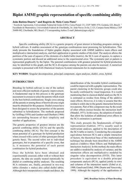
Crop Breeding and Applied Biotechnology, v. 2, n. 2, p. 161-170, 2002161Biplot AMMI graphic representation of specific combining abilityJoão Batista Duarte *1 and Rogério de Melo Costa Pinto 21Escola de Agronomia, Universidade Federal de Goiás (UFG), Caixa Postal 131, CEP 74001-970, Goiânia, GO, Brazil; 2Faculdade de Matemática, Universidade Federal de Uberlândia, Av. João Naves Ávila, 2.121, Campus Santa Mônica, CEP38400-902, Uberlândia, MG, Brazil. (* Corresponding Author. E-mail: jbduarte@agro.ufg.br)ABSTRACTSpecific combining ability (SCA) is a genetic property of great interest in breeding programs aiming athybrid cultivars. It enables assessment of the genotype combinations most promising for hybridization. Thisstudy presents the foundations of biplot graphic display associated with AMMI (additive main effects andmultiplicative interaction) analysis, and their application to genetic studies of this kind. The analysis allows thepartition of the sum of squares of the elements of a diallel table (matrix), the SCA sum of squares, to capture asystematic portion and discard an additional noise to the experimental error. The systematic part or pattern isrepresented graphically by the biplot. The parental combinations with greatest potential for hybrid productionmay be identified in this graph, and the SCA divergence among the parents can also be assessed. A numericalexample is presented with SAS (Statistical Analysis System) statements for its implementation.KEY WORDS: Singular decomposition, principal component, eigen analyses, diallel, cross, hybrid.INTRODUCTIONBreeding for hybrid cultivars is one of the earliestand most efficient methods of genetic improvement.A fundamental step in this process is the genotypeassessment in crosses to select the parents which resultin the best hybrid combinations. Single cross amongall the parents or among those of known diverse originmust be obtained for this purpose. Diallel crosses havebeen designed to assess the properties of the parentssubmitted to hybridization. The methods proposedby Griffing (1956) and Gardner and Eberhart (1966)are outstanding because of their simplicity andnumber of applications.The genetic properties of greatest interest are thegeneral combining ability (GCA) and the specificcombining ability (SCA). The first concept is themean potential of a genotype for hybrid productionwhen crossed with a series of other genotypes (broadgenetic base). The second refers not to individualgenotypes, but to properties of a specific cross, thatis, it measures the potential of each parentcombination for hybrid production.Once the hybrids have been obtained andexperimentally assessed, either with or without theirparents, the data are usually treated statistically bydiallel or combining ability analyses. The resultingSCA estimates are, finally, presented in two-waytables (females x males) also called diallel tables.Although their interpretation is simple and direct, theidentification of the favorable hybrid combinationscould be improved with a graphic representation. Theparent clustering in the heterotic groups could alsobe easily confirmed by visual inspection. It is worthmentioning that in classical diallel analyses the SCAis estimated as residue from fitting of the additivemain effects. However, it is risky to assume that thisresidue is solely due to the genetic interaction betweentwo parents. Part of this component may be the resultof other effects (noise) besides the interaction itself(Mandel, 1971). In this sense, the adoption of modelsthat allow the isolation of additional error effects inthe SCA estimation is pertinent.This study presents the fundamentals of biplotrepresentation (Gabriel, 1971), usually used inmultivariate analyses, applied to the description ofthe SCA table or matrix. Considering the conceptualequivalence between SCA and a simple interactionof factors, the theoretical base of this mathematicaltechnique has already been described in the AMMIanalysis (Additive Main Effects and MultiplicativeInteraction Analysis). In this method, the main effectsare additive modeled by analysis of variance, and theinteraction effects are multiplicative modeled bysingular value decomposition (SVD). This latterprocedure is equivalent to a double principalcomponents analysis (PCA), applied jointly to rowsand columns of the interaction matrix (Zobel et al.,1988; Gauch and Zobel, 1996; Duarte and Vencovsky,1999). Although the majority of the applications of2002, Brazilian Society of Plant Breeding

162 Crop Breeding and Applied Biotechnology, v. 2, n. 2, p. 161-170, 2002this analysis are related to genotype x environmentinteraction (GEI) studies, the authors suggest its perfectadaptation to line assessment in test crossings, such asthe diallel crosses.METHODOLOGYSingular value decompositionThe biplot graphic display is based on a matrix algebratool called singular value decomposition (SVD).Proposed by Eckart and Young (1936), this procedureallows writing a real matrix B, of rank p, as a sum ofp orthogonal unitary rank matrices:B (lxc) =p∑ λ kk=1u k v k ’where: k=1, 2, ..., p and p ≤ min{l , c}and λ kis the k th singular value of B (the square rootof the k th non-zero eigenvalue of BB’ or B’B), and u kand v k’ are the associated singular vectors, columnvector and row vector respectively.When the sum for k is applied only to the n first terms(with n

Crop Breeding and Applied Biotechnology, v. 2, n. 2, p. 161-170, 2002163only the few first terms (one, two or three) alreadydescribe a high proportion of this sum of squares. Thisallows the description of the SCA using a parsimoniousmodel (in the sense of using few degrees of freedom)and with good capacity to explain the original variabilitypresent in the matrix. Therefore, the analysis allowsa interpretation of the SS SCAby an approximation ofrank n of the SCA matrix. As n is possibly smallerthan p (e.g. n =1, 2 or 3) the analysis results in aninformative model which can be representedgraphically, since a complex p-dimensional space isrepresented in a bi or tridimensional graph.In the context of the AMMI method, the objective ofthe analysis is to describe the interaction by a reducednumber of axes. It is expected that, successively, eachaxis will capture a smaller portion of the patternunderlying to the interaction (general law whichgoverns the phenomena) and more noise present inthe data. Thus, a simpler model would discard a highproportion of noise which has no agronomic interestand can hamper good predictions, retaining mainlythe portion rich in deterministic information (Gauchand Zobel, 1988; Gauch, 1990). This separation inpattern and noise effects may also be expressed interms of sum of squares:p222SS SCA = ∑ λ = ( ∑ λ ) + ( ∑ λ )nkkkk= 1 k= 1 k= n+1= (SS SCA_pattern) + (SS SCA_noise).The biplot graphic displayAn important property of the SVD approximation isits allowance for the representation of effects of eachrow and of each column in a single graph calledbiplot. The name does not come from the spacedimension of representation, but from the fact that itdisplays simultaneously the rows and the columns ofthe matrix.To understand the mathematical origin of a biplotconsider the SVD n-approximation for the B matrixof rank p>n: ˆn ~~ ~ ~B( fxm)= ∑ k= 1 λkukv′k= USV′; where U( fxn)has~in its columns only the n first u (fx1)vectors; V ′( nxm)has~in its rows the n first v’ (1xm)vectors; and S( n)is thediagonal matrix with the first singular values,λ 1,λ 2,...,λ n(Duarte and Vencovsky, 1999). Theexpression may further be written as:Bˆ =~~ 1/ 2 ~ 1/ 2 ~( U S )( S V ′); or simply Bˆ =~ ~( G )( H ′), where~G( fxn)=~~ 2~( U S1/ ) and H ′( nxm)= ~ 1/ 2 ~( S V ′). Thus, ~ G matrixwill have f vectors called row markers, each one withn elements, the coordinates of the females (F) forpeach singular axis selected. Similarly, ~ H ′ will have mcolumn markers, each also with n elements,corresponding to the male (M) coordinates for thesame n axes. Given that these axes are orthogonal,the f females and m males can be plotted in a singlecartesian system of n perpendicular axes. In practice,similar to the scatter plots in PCA, the rank of theapproximate matrix (n) to be displayed should be one,two or three, which would allow a graphicrepresentation in one, two or three dimensions,respectively.A property of biplot representation is that any elementof the approximate matrix is exactly the inner productof the vectors (markers) corresponding to its row andto its column (Gabriel, 1971). In this case, the productbetween the coordinates of the i th female and the j thmale yields the expected SCA value for that hybridcombination ( ŝAMMIij ). Clearly, this value does notcorrespond to that in the diallel table because thebiplot represents the SVD n-approximation of theoriginal B matrix. However, it is expected that thisprediction, rich in pattern, is closer to the real SCA(s ij) than the values ŝ ij of the diallel table, which arepotentially rich in noise (Gauch, 1990). In this sense,a male/female pair with coordinates of highmagnitude and the same signal has high SCA (positiveinteraction), characterizing a favorable combinationfor hybridization. On the other hand, a combinationwhose coordinates have opposite signs and negativeSCA is unfavorable. Thus the intergroup genotypedistances (F/M) have inverse interpretation in relationto the distance visualized in the graph, that is, pointsclose together do not indicate genotypic similarity butrather affinity for hybrid combination.On the other hand, inspecting only the female (ormale) markers, it is possible to assess the intragroupdivergences. In this case, close points indicate greatergenotypic similarity. In complete diallels, the femalesand males are the same genotypes and, therefore, suchinspection would enable the assessment of thedivergence among all the parents. Thus for genotypeclustering, it would be enough to plot only the femalemarkers (or the males) as in PCA display. However,in this case the opportunity to graphically predict theSCA magnitude and to identify the most promisinghybrid combinations would be lost.APPLICATIONTo illustrate the use of the biplot graphic display inSCA description, Griffing (1956) method IV results2002, Brazilian Society of Plant Breeding

164 Crop Breeding and Applied Biotechnology, v. 2, n. 2, p. 161-170, 2002(diallel with F1 hybrids, without parents and reciprocals) were taken. The ŝij estimates for grain yield in maizeare expressed by the symmetric B (9x9)matrix (F indicates females, and M, males):M1 M2 M3 M4 M5 M6 M7 M8 M9B =0.00 4.94 14.46 -2.76 2.80 -12.31 -16.93 -8.67 18.47 F14.94 0.00 -6.54 14.14 8.90 5.68 13.07 -2.47 -37.73 F214.46 -6.54 0.00 -29.94 19.01 15.80 4.48 -6.96 -10.31 F3-2.76 14.14 -29.94 0.00 11.50 -8.21 3.77 -19.47 30.97 F42.80 8.90 19.01 11.50 0.00 -36.16 -0.77 4.99 -10.27 F5-12.31 5.68 15.80 -8.21 -36.16 0.00 -10.78 32.77 13.22 F6-16.93 13.07 4.48 3.77 -0.77 -10.78 0.00 5.66 1.50 F7-8.67 -2.47 -6.96 -19.47 4.99 32.77 5.66 0.00 -5.85 F818.47 -37.73 -10.31 30.97 -10.27 13.22 1.50 -5.85 0.00 F9The matrix symmetry comes from the assumption ofno reciprocal effects, although the analysis issufficiently generic to accommodate non-symmetricmatrices. The SCA mean square is 339.44, with27 degrees of freedom, which corresponds to:SS SCA=9164.28 (Griffing, 1956). The SS of the matrixelements ( ∑ 2 2bij= ∑ $s ij= 18328.55) is then equivalent totwice the SS SCA( ŝ ij values repeated above and belowthe main diagonal). Therefore, the partition of the sumof square of the matrix elements corresponds topartitioning the SS SCA.As mentioned earlier, the SVD decomposition of theB matrix is: B=USV’. The U, S and V matrices, thatdetermine this partition, can be obtained using acomputer program for matrix algebra. The Proc IML(interactive matrix language procedure) of theSAS (Statistical Analysis System) can be used, forexample, with the syntax “call svd (U,S,V,B);”. Theresults of the application of this command are thematrices:i) U (9x8)matrix of singular vectors associated with rows (females):0.2640 0.1759 -0.1622 0.0515 0.5091 0.5569 0.4353 -0.0210-0.3450 -0.3612 -0.0589 -0.4124 -0.3872 0.0198 0.5486 -0.1207-0.3671 0.2619 0.2526 -0.2661 0.5169 -0.3951 -0.1281 -0.3335-0.0160 0.5778 -0.5138 0.2488 -0.3196 -0.3324 0.1029 0.0760U = 0.3470 -0.3116 -0.2969 -0.4184 0.1818 -0.2327 -0.2924 0.48530.5286 -0.1209 0.5549 0.2996 -0.1352 -0.3438 0.2396 -0.05660.2452 0.0337 -0.0381 -0.1533 -0.3288 0.3567 -0.5120 -0.5524-0.3097 0.2535 0.4556 0.0130 -0.1937 0.3505 -0.1962 0.5676-0.3470 -0.5090 -0.1933 0.6373 0.1566 0.0201 -0.1975 -0.0446ii) S (8)matrix of singular values:S = diag {77.1865 63.3445 60.1728 54.7776 36.8391 17.6392 8.1048 1.7241}iii) V’ (8x9)matrix of singular vectors associated with columns (males):-0.2640 0.3450 0.3671 0.0160 -0.3470 -0.5286 -0.2452 0.3097 0.3470-0.1759 0.3612 -0.2619 -0.5778 0.3116 0.1209 -0.0337 -0.2535 0.5090-0.1622 -0.0589 0.2526 -0.5138 -0.2969 0.5549 -0.0381 0.4556 -0.1933V’ = 0.0515 -0.4124 -0.2661 0.2488 -0.4184 0.2996 -0.1533 0.0130 0.63730.5091 -0.3872 0.5169 -0.3196 0.1818 -0.1352 -0.3288 -0.1937 0.1566-0.5569 -0.0198 0.3951 0.3324 0.2327 0.3438 -0.3567 -0.3505 -0.02010.4353 0.5486 -0.1281 0.1029 -0.2924 0.2396 -0.5120 -0.1962 -0.19750.0210 0.1207 0.3335 -0.0760 -0.4853 0.0566 0.5524 -0.5676 0.04462002, Brazilian Society of Plant Breeding

Crop Breeding and Applied Biotechnology, v. 2, n. 2, p. 161-170, 2002165Note that the S matrix of non-null singular values isof 8x8 dimension indicating that the rank of B is alsop=8, which corresponds to the number of parentsminus one. Thus the SS SCAmay be partitioned in upto eight components (IPCA axes) as shown in Table1. In the present case (complete diallel), eachcomponent corresponds to half the square of eachsingular value, that is: SS SCA(IPCAk)=( λ 2 k)/2, withk=1,2,...,8. In the partial diallels (non-symmetricmatrices and possibly rectangular matrices) thepartition is direct, without division by two. In thisexample, the biplot representation of the SCA isillustrated taking the first three singular axes.Before constructing the biplot graphic display it isnecessary to obtain the G and H’ matrices, such thatG=US 1/2 and H’=S 1/2 V’ (so that B=GH’):i) G (9x8)matrix of row markers (females F1, F2, ...., F9):G =2.3198 1.4001 -1.2579 0.3811 3.0903 2.3389 1.2392 -0.0276 F1-3.0311 -2.8750 -0.4565 -3.0524 -2.3502 0.0834 1.5617 -0.1585 F2-3.2249 2.0848 1.9591 -1.9692 3.1374 -1.6595 -0.3646 -0.4379 F3-0.1409 4.5983 -3.9856 1.8411 -1.9398 -1.3960 0.2928 0.0998 F43.0482 -2.4803 -2.3030 -3.0966 1.1035 -0.9773 -0.8325 0.6372 F54.6443 -0.9626 4.3047 2.2172 -0.8207 -1.4441 0.6821 -0.0743 F62.1540 0.2680 -0.2958 -1.1342 -1.9958 1.4980 -1.4577 -0.7254 F7-2.7205 2.0173 3.5341 0.0964 -1.1755 1.4722 -0.5587 0.7452 F8-3.0488 -4.0508 -1.4991 4.7167 0.9508 0.0844 -0.5623 -0.0585 F9ii) H’ (8x9)matrix of column markers (males: M1, M2,...M9):H’=M1 M2 M3 M4 M5 M6 M7 M8 M9-2.3198 3.0311 3.2249 0.1409 -3.0482 -4.6443 -2.1540 2.7205 3.0488-1.4001 2.8750 -2.0848 -4.5983 2.4803 0.9626 -0.2680 -2.0173 4.0508-1.2579 -0.4565 1.9591 -3.9856 -2.3030 4.3047 -0.2958 3.5341 -1.49910.3811 -3.0524 -1.9692 1.8411 -3.0966 2.2172 -1.1342 0.0964 4.71673.0903 -2.3502 3.1374 -1.9398 1.1035 -0.8207 -1.9958 -1.1755 0.9508-2.3389 -0.0834 1.6595 1.3960 0.9773 1.4441 -1.4980 -1.4722 -0.08441.2392 1.5617 -0.3646 0.2928 -0.8325 0.6821 -1.4577 -0.5587 -0.56230.0276 0.1585 0.4379 -0.0998 -0.6372 0.0743 0.7254 -0.7452 0.0585The dotted rows in G and H’ delimit at the left andabove the G ~ and H ~ ′ matrices, respectively, and thecoordinates corresponding to females and to malesfor the construction of a three dimensional biplot(biplot-AMMI3). This representation captures74.15% of the original SS SCA(Table 1) and thepredominant pattern associated with the SCA. Thus,it is expected that the SCA predictions obtained bythe SVD 3-approximation ( Bˆ ~ ~ =G H ′) should be morerealistic than those presented in the original diallel table(matrix B). If only the first two columns of G and thefirst two rows of H’ were taken, the biplot would berepresented in a plan (biplot-AMMI2); however, itwould explain only 54.40% of the SS SCA. Finally, theAMMIŝij values predicted by the SVD 3-approximationof the B matrix are expressed by:M1 M2 M3 M4 M5 M6 M7 M8 M9-5.76 11.63 2.10 -1.10 -0.70 -14.84 -5.00 -0.96 14.63 F111.63 -17.24 -4.68 14.61 3.16 9.35 7.43 -4.06 -20.20 F2Bˆ =2.10 -4.68 -10.91 -17.85 10.49 25.42 5.81 -6.06 -4.32 F3-1.10 14.61 -17.85 -5.28 21.01 -12.08 0.25 -23.74 24.17 F4-0.70 3.16 10.49 21.01 -10.14 -26.46 -5.22 5.16 2.70 F5-14.84 9.35 25.42 -12.08 -26.46 -3.97 -11.02 29.79 3.81 F6-5.00 7.43 5.81 0.25 -5.22 -11.02 -4.62 4.27 8.10 F7-0.96 -4.06 -6.06 -23.74 5.16 29.79 4.27 1.02 -5.42 F814.63 -20.20 -4.32 24.17 2.70 3.81 8.10 -5.42 -23.46 F92002, Brazilian Society of Plant Breeding

166 Crop Breeding and Applied Biotechnology, v. 2, n. 2, p. 161-170, 2002Considering the observed high correlation between Bˆand B ( r = 0.74 = 0. 86) it can be said that in thisexample the error associated with a decision based on Binstead of on Bˆ would not be great. It is justifiedbecause, under an adequate choice of the number ofmultiplicative terms (or singular axes), a low magnitudecorrelation between Bˆ and B is related to thepredominance of noise in the B matrix. Thus, in thissituation, it may be wrong to interpret the residues ŝ ijas reliable estimates of the true SCA (s ij).Based on the Bˆ matrix the following crosses wereoutstanding among the more favorable combinations:6x8, 3x6, 4x9 and 4x5 (female x male or vice-versa).Also, note that in the case of complete diallels andunder the assumption of no reciprocal effects, the SCAprediction matrix is also symmetric. Further, the SCAof each parent with itself (s jj) is estimated, allowinginferences on varietal heterosis (Cruz and Vencovsky,1989). The majority of these values were negative,indicating that this type of cross is not adequate forhybrid extraction. The parents identified by thenumbers 8, 6 and 7, in this order, should show greatervarietal heterosis than those of the numbers 9 and 2.Further note that, in spite of the arbitrariness of theassignment of zero values for the main diagonalelements of B, the analysis was able to predict thedistinct reaction of the parents when crossed withthemselves. This opens the perspective of predictingthe SCA from unavailable crosses, avoiding the needto assess all possible single crosses.The possibility of predicting the hybrid performanceof non-realized crosses comes from the fact that theanalysis deals with the interaction (SCA) not only as aproperty of each parental combination, but also in anintegrated manner, as a phenomenon determinedtogether by rows and columns of the B matrix.However, if the major interest is for this type ofprediction, it is recommended that one proceedsinteractively according to Gauch (1992). Furthermore,to predict the genotypic responses it is necessary totake into account the main effects associated with eachparent. Charcosset et al. (1993) used models withmultiplicative interaction terms (AMMI analysis) witha similar purpose of predicting the performance of linehybrids in maize, when the assessment of all the singlecrosses were not possible. The authors concluded thatthe models offer the possibility of improving predictionefficiency, without supplementary measurements. Theproblem could also be treated by the mixed modelsapproach, obtaining the BLUP (best linear unbiasedpredictor) of the s ijof missing hybrids (Bernardo, 1996;André, 1999), followed by the SVD adjustment of thesepredictions.The coordinates of each parent, used to construct thegraphics, are summarized in Table 2. A SAS programto execute the analysis is freely available from theweb-address: www.agro.ufg.br.The relationships commented upon may be seen bylooking at the corresponding biplot. Figure 1, althoughbringing all the biplot-AMMI3 information, does notallow a perfect assessment of the relative distancesamong the parents because it is a three dimensionalgraph projected on the paper plane. Thus, for a morerigorous inspection, it is convenient to project the pointsof the 3-D space in at least two complementary planes,for example, IPCA1 vs. IPCA2 and IPCA1 vs. IPCA3(Figure 2). Therefore, the closeness between two points(genotypes) must always be confirmed by inspectionin these principal planes.Figures 1 and 2 summarize the potential of thedifferent parental combinations to produce hybrids.These graphics do not explain the whole SCA value.However, according to the AMMI analysis concept(as in PCA), the true pattern of interaction (SCA) isTable 1. The partition of SS SCA(specific combining ability sum of the squares) by singular decomposition, proportionretained in each singular axis and accumulated percentage up to k th axis, in a diallel AMMI analysis.IPCA k SS IPCAk SS IPCAk /SS SCA % Accumulated1 2978.8753 0.3251 32.50532 2006.2649 0.2189 54.39753 1810.3817 0.1975 74.15234 1500.2918 0.1637 90.52345 678.5611 0.0740 97.92786 55.5711 0.0170 99.62547 32.8437 0.0036 99.98388 1.4862 0.0002 100.0000Total 9164.2760 1.0000 -2002, Brazilian Society of Plant Breeding

Crop Breeding and Applied Biotechnology, v. 2, n. 2, p. 161-170, 2002167described mainly by the first singular axes. Each axisis a linear combination of the rows and columns(vectors) which form the B matrix. As all these vectorscontain ŝij values, the axes represent SCA linearfunctions constructed with all the matrix data. Finally,as the successive axes capture ever less pattern andmore noise, discarding the latter becomes necessaryto avoid the incorporation of substantial errors in thedescription of the interaction.Conscious of these concepts and observing the pairsof points corresponding to each female and malecombination, the proximity between F6/M3, F6/M8,F4/M9 and F4/M5 can be depicted. This indicatesthat such combinations are promising for single crossproduction in this set of parents. A strongcharacteristic in all of them is the high magnitudeand same sign coordinates for the genotypes of eachpair. On the other hand, it can be deduced that thegenotypes with good GCA should have lowmagnitude coordinates (small interaction) as is thecase of parents 1 and 7 (Figure 1). These lines areshown to have high GCA in Griffing analysis (1956).Among the combinations with lower potential forhybrid production are: F2/M9, F6/M5 and F4/M8,all showing great distance among the respective F/Mpoints in the Figures 1 and 2. Further, the low potentialis also observed for crosses among the same genotype(F6/M6, F9/M9, etc.), which always show points inopposite position. It is interesting to note that theF3xM5 cross although shown as fairly favorable inTable 2. Coordinates of the parents for the three firstprincipal axes (IPCA1, IPCA2 and IPCA3) of a biplotgraphic display, in a diallel AMMI analysis.Point Female/Male IPCA 1 IPCA 2 IPCA 31 F1 2.3197 1.4001 -1.25792 F2 -3.0311 -2.8749 -0.45653 F3 -3.2249 2.0848 1.95914 F4 -0.1408 4.5982 -3.98555 F5 3.0481 -2.4802 -2.30306 F6 4.6443 -0.9625 4.30467 F7 2.1540 0.2680 -0.29588 F8 -2.7205 2.0172 3.53419 F9 -3.0488 -4.0507 -1.499010 M1 -2.3197 -1.4001 -1.257911 M2 3.0311 2.8749 -0.456512 M3 3.2249 -2.0848 1.959113 M4 0.1408 -4.5982 -3.985514 M5 -3.0481 2.4802 -2.303015 M6 -4.6443 0.9625 4.304616 M7 -2.1540 -0.2680 -0.295817 M8 2.7205 -2.0172 3.534118 M9 3.0488 4.0507 -1.4990Figure 1. Biplot AMMI3 for specific combiningability (SCA) in maize grain yield of a diallel cross;the cubes identify female genotypes (F), and thepyramids, the male genotypes (M).the original diallel table, was shown to be onlyreasonable by the present analysis. This happenedbecause the AMMI method discards part of theinformation contained in the original matrix as ofpredominantly erratic in nature. The option for thebiplot-AMMI3 implied in disregarding 26% of theSS SCA. These results can be confirmed in the Bˆmatrix for ŝ AMMIij prediction.When only one kind of marker is taken, for examplethe F points (or the M points), the divergences andsimilarities among the genotypes which make up theparent group can be assessed. Thus the divergencebetween genotypes 3 and 6 is notorious, as well asthose between 4 and 9. However, it is also evidentthe similarity between the genotypes 3 and 8, andbetween 2 and 9 (Figures 1 and 2). Observe also thatthe first principal axis (IPCA1), capturing 32% ofthe SCA, is strongly determined by the divergenceamong two groups of genotypes (2, 3, 8, 9) and (1, 5,6, 7). The two best hybrid combinations foundresulted exactly from the cross between genotypesbelonging to distinct groups (3x6 and 6x8). The twoother axes, each explaining about 20% of the referredvariability, relate more with intragroup genotypicdivergences. Therefore, the biplot display was shownto be an additional tool to guide the formation ofheterotic groups and the planning of future crosses.CONCLUSIONSThe adoption of biplot-AMMI to represent the SCAallows a quick visualization of the favorable andunfavorable genotypic combinations for hybridproduction. The use of this graphic display also allowsa quick and easy assessment of the genotypicdivergences and similarities among the parents2002, Brazilian Society of Plant Breeding

168 Crop Breeding and Applied Biotechnology, v. 2, n. 2, p. 161-170, 2002Figure 2. Two first principal planes for specific combining ability (SCA) in maize grain yield of a diallel cross;F (females) identify the genotypes in the rows and M (males) the genotypes in the columns of the diallel table.involved in the diallel crosses. Further, the possibilityof discarding an additional noise may guaranteeimprovements in estimates of SCA.Considering the integrated treatment which theAMMI analysis offers to the data, it is possible topredict the SCA, even for hybrid combinations notassessed experimentally. This opens the perspectiveof incorporating this method of analysis, associatedwith biplot representation, in the routine proceduresof prediction of hybrid means in breeding programs.RESUMORepresentação gráfica BIPLOT-AMMI para acapacidade específica de combinaçãoNo melhoramento para a obtenção de híbridos, umapropriedade genética de grande interesse é acapacidade específica de combinação (CEC).Através dela é possível avaliar as combinações degenótipos mais promissoras à hibridação. O presentetrabalho tem o objetivo de apresentar os fundamentosda representação biplot, associada à análise AMMI(additive main effects and multiplicativeinteraction), bem como sua aplicação aos estudosgenéticos dessa natureza. A análise permite umadecomposição da soma de quadrados dos elementosda tabela (matriz) dialélica, a soma de quadrados paraCEC, de maneira a captar uma porção sistemática edescartar um resíduo adicional ao erro doexperimento. A parte sistemática ou padrão é, então,representada graficamente por meio do biplot. Nestegráfico pode-se identificar as combinações degenitores com maior potencialidade para a produçãode híbridos, bem como avaliar a divergência entre osparentais, em termos de CEC. Um exemplo numéricoé apresentado com instruções computacionais para asua implementação.REFERENCESAndré, C.M.G. 1999. Avaliação da melhor prediçãolinear não tendenciosa BLUP associada ao uso demarcadores moleculares na análise dialética. M.S.Thesis. Universidade Federal de Lavras, Lavras.Bernardo, R. 1996. Best linear unbiased prediction ofmaize single-cross performance. Crop Science. 36:50-56.Charcosset, A.; Denis, J.B.; Lefort-Buson, M. andGallais, A. 1993. Modelling interaction from topcrossdesign data and prediction of F1 hybrid value.Agronomie. 13:597-608.Cruz, C.D. and Vencovsky, R. 1989. Comparision ofsome methods of diallel analysis. Revista Brasileirade Genetica. 12:425-438.Duarte, J.B. and Vencovsky, R. 1999. Interaçãogenótipos x ambientes, uma introdução à análiseAMMI. Série Monografias, n.9. Sociedade Brasileirade Genética, Ribeirão Preto.Eckart, C. and Young, G. 1936. The approximationof one matrix by another of lower rank.Psychometrika. 1:211-218.Gabriel, K.R. 1978. Least squares approximation ofmatrices by additive and multiplicative models. J.R. Statist. Soc. 40:186-196.Gabriel, K.R. 1971. The biplot graphic display ofmatrices with application to principal componentanalysis. Biometrika. 58:453-467.Gardner, C.O. and Eberhart, S.A. 1966. Analysis and2002, Brazilian Society of Plant Breeding

Crop Breeding and Applied Biotechnology, v. 2, n. 2, p. 161-170, 2002169interpretation of the variety cross diallel and relatedpopulations. Biometrics. 22:439-452.Gauch, H.G. 1990. Full and reduced models for yieldtrials. Theoretical Applied Genetics. 80:153-160.Gauch, H.G. and Zobel, R.W. 1996. AMMI analysisof yield trials. p.85-122. In: Kang, M.S. and Gauch,H.G.(Eds.). Genotype by environment interaction.CRC Press, Boca Raton.Gauch, H.G. and Zobel, R.W. 1988. Predictive andpostdictive success of statistical analysis of yieldtrials. Theoretical Applied Genetics. 76:1-10.Gauch, H.G. 1992. Statistical analysis of regionalyield trials: AMMI analysis of factorial designs.Elsevier, New York.Gollob, H.F. 1968. A statistical model whichcombines features of factor analytic and analysis ofvariance techniques. Psychometrika. 33:73-115.Good, I.J. 1969. Some applications of the singulardecomposition of a matrix. Technometrics. 11:823-831.Griffing, B. 1956. Concept of general and specificcombining ability in relation to diallel crossingsystems. Austr. J. Biol. Sci. 9:463-493.Mandel, J. 1971. A new analysis of variance modelfor non-additive data. Technometrics. 13:1-18.Zobel, R.W.; Wright, M.J. and Gauch, H.G. 1988.Statistical analysis of a yield trial. Agronomy Journal.80:388-393.Received: August 20, 2001;Accepted: May 23, 2002.2002, Brazilian Society of Plant Breeding

170 Crop Breeding and Applied Biotechnology, v. 2, n. 2, p. 161-170, 20022002, Brazilian Society of Plant Breeding