Genetic Drift - Kent Holsinger

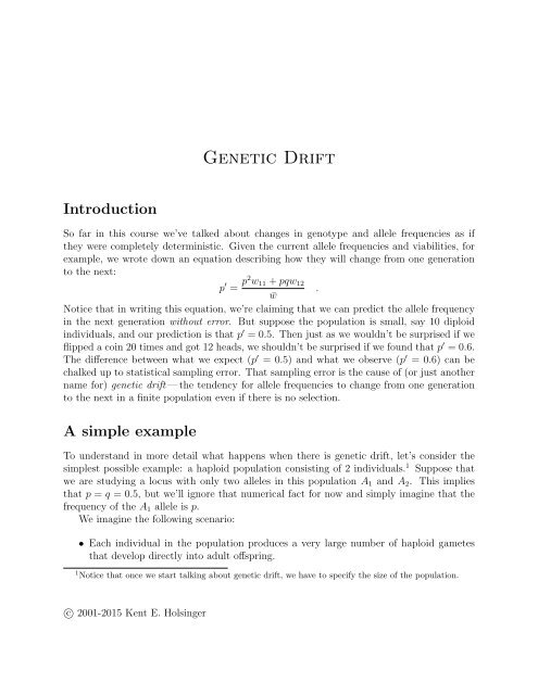
Genetic DriftIntroductionSo far in this course we’ve talked about changes in genotype and allele frequencies as ifthey were completely deterministic. Given the current allele frequencies and viabilities, forexample, we wrote down an equation describing how they will change from one generationto the next:p ′ = p2 w 11 + pqw 12.¯wNotice that in writing this equation, we’re claiming that we can predict the allele frequencyin the next generation without error. But suppose the population is small, say 10 diploidindividuals, and our prediction is that p ′ = 0.5. Then just as we wouldn’t be surprised if weflipped a coin 20 times and got 12 heads, we shouldn’t be surprised if we found that p ′ = 0.6.The difference between what we expect (p ′ = 0.5) and what we observe (p ′ = 0.6) can bechalked up to statistical sampling error. That sampling error is the cause of (or just anothername for) genetic drift — the tendency for allele frequencies to change from one generationto the next in a finite population even if there is no selection.A simple exampleTo understand in more detail what happens when there is genetic drift, let’s consider thesimplest possible example: a haploid population consisting of 2 individuals. 1 Suppose thatwe are studying a locus with only two alleles in this population A 1 and A 2 . This impliesthat p = q = 0.5, but we’ll ignore that numerical fact for now and simply imagine that thefrequency of the A 1 allele is p.We imagine the following scenario:• Each individual in the population produces a very large number of haploid gametesthat develop directly into adult offspring.1 Notice that once we start talking about genetic drift, we have to specify the size of the population.c○ 2001-2015 Kent E. Holsinger

• The allele in each offspring is an identical copy of the allele in its parent, i.e., A 1 begetsA 1 and A 2 begets A 2 . In other words, there’s no mutation.• The next generation is constructed by picking two offspring at random from the verylarge number of offspring produced by these two individuals.Then it’s not too hard to see thatProbability that both offspring are A 1 = p 2Probability that one offspring is A 1 and one is A 2 = 2pqProbability that both offspring are A 2 = q 2Of course p ′ = 1 if both offspring sampled are A 1 , p ′ = 1/2 if one is A 1 and one is A 2 , andp ′ = 0 if both are A 2 , so that set of equations is equivalent to this one:P (p ′ = 1) = p 2 (1)P (p ′ = 1/2) = 2pq (2)P (p ′ = 0) = q 2 (3)In other words, we can no longer predict with certainty what allele frequencies in the nextgeneration will be. We can only assign probabilities to each of the three possible outcomes.Of course, in a larger population the amount of uncertainty about the allele frequencieswill be smaller, 2 but there will be some uncertainty associated with the predicted allelefrequencies unless the population is infinite.The probability of ending up in any of the three possible states obviously depends onthe current allele frequency. In probability theory we express this dependence by writingequations (1)–(3) as conditional probabilities:P (p 1 = 1|p 0 ) = p 2 0 (4)P (p 1 = 1/2|p 0 ) = 2p 0 q 0 (5)P (p 1 = 0|p 0 ) = q 2 0 (6)I’ve introduced the subscripts so that we can distinguish among various generations in theprocess. Why? Because if we can write equations (4)–(6), we can also write the followingequations: 3 P (p 2 = 1|p 1 ) = p 2 1P (p 2 = 1/2|p 1 ) = 2p 1 q 1P (p 2 = 0|p 1 ) = q 2 12 More about that later.3 I know. I’m weird. I actually get a kick out of writing equations!2

Now if we stare at those a little while, we 4 begin to see some interesting possibilities.Namely,P (p 2 = 1|p 0 ) = P (p 2 = 1|p 1 = 1)P (p 1 = 1|p 0 ) + P (p 2 = 1|p 1 = 1/2)P (p 1 = 1/2|p 0 )= (1)(p 2 0) + (1/4)(2p 0 q 0 )= p 2 0 + (1/2)p 0 q 0P (p 2 = 1/2|p 0 ) = P (p 2 = 1/2|p 1 = 1/2)P (p 1 = 1/2|p 0 )= (1/2)(2p 0 q 0 )= p 0 q 0P (p 2 = 0|p 0 ) = P (p 2 = 0|p 1 = 0)P (p 1 = 0|p 0 ) + P (p 2 = 0|p 1 = 1/2)P (p 1 = 1/2|p 0 )= (1)(q 2 0) + (1/4)(2p 0 q 0 )= q 2 0 + (1/2)p 0 q 0It takes more algebra than I care to show, 5arbitrary number of generations.but these equations can be extended to anP (p t = 1|p 0 ) = p 2 0 + ( 1 − (1/2) t−1) p 0 q 0P (p t = 1/2|p 0 ) = p 0 q 0 (1/2) t−2P (p t = 0|p 0 ) = q 2 0 + ( 1 − (1/2) t−1) p 0 q 0Why do I bother to show you these equations? 6 Because you can see pretty quickly thatas t gets big, i.e., the longer our population evolves, the smaller the probability that p t = 1/2becomes. In fact, it’s not hard to verify two facts about genetic drift in this simple situation:1. One of the two alleles originally present in the population is certain to be lost eventually.2. The probability that A 1 is fixed is equal to its initial frequency, p 0 , and the probabilitythat A 2 is fixed is equal to its initial frequency, q 0 .Both of these properties are true in general for any finite population and any number ofalleles.1. Genetic drift will eventually lead to loss of all alleles in the population except one. 74 Or at least the weird ones among us5 Ask me, if you’re really interested.6 It’s not just that I’m crazy.7 You obviously can’t lose all of them unless the population becomes extinct.3

2. The probability that any allele will eventually become fixed in the population is equalto its current frequency.General properties of genetic driftWhat I’ve shown you so far applies only to a haploid population with two individuals. EvenI will admit that it isn’t a very interesting situation. Suppose, however, we now considera populaton with N diploid individuals. We can treat it as if it were a population of 2Nhaploid individuals using a direct analogy to the process I described earlier, and then thingsstart to get a little more interesting.• Each individual in the population produces a large number of gametes.• The allele in each gamete is an identical copy of the allele in the individual thatproduced it, i.e., A 1 begets A 1 and A 2 begets A 2 .• The next generation is constructed by picking 2N gametes at random from the largenumber originally produced.We can then write a general expression for how allele frequencies will change betweengenerations. Specifically, the distribution describing the probability that there will be jcopies of A 1 in the next generation given that there are i copies in this generation is( 2NP (j A 1 in offspring | i A 1 in parents) =j) ( ) ( i1 − i )2N 2Ni.e., a binomial distribution. I’ll be astonished if any of what I’m about to say is apparentto any of you, but this equation implies three really important things. We’ve encounteredtwo already:• Allele frequencies will tend to change from one generation to the next purely as a resultof sampling error. As a consequence, genetic drift will eventually lead to loss of allalleles in the population except one.• The probability that any allele will eventually become fixed in the population is equalto its current frequency.,4

• The population has no memory. 8 The probability that the offspring generation willhave a particular allele frequency depends only on the allele frequency in the parentalgeneration. It does not depend on how the parental generation came to have that allelefrequency. This is exactly analogous to coin-tossing. The probability that you get aheads on the next toss of a fair coin is 1/2. It doesn’t matter whether you’ve nevertossed it before or if you’ve just tossed 25 heads in a row. 9Variance of allele frequencies between generationsFor a binomial distributionApplying this to our situation,P (K = k) =( Nk)Var(K) = Np(1 − p)p k (1 − p) N−kVar(p) = Var(K/N)= 1N Var(K)2p(1 − p)=NVar(p t+1 ) = p t(1 − p t )2NVar(p t+1 ) measures the amount of uncertainty about allele frequencies in the next generation,given the current allele frequency. As you probably guessed long ago, the amountof uncertainty is inversely proportional to population size. The larger the population, thesmaller the uncertainty.If you think about this a bit, you might expect that a smaller variance would “slowdown” the process of genetic drift — and you’d be right. It takes some pretty advancedmathematics to say how much the process slows down as a function of population size, 10 butwe can summarize the result in the following equation:¯t ≈ −4N (p log p + (1 − p) log(1 − p)) ,8 Technically, we’ve described a Markov chain with a finite state space, but I doubt that you really careabout that.9 Of course, if you’ve just tossed 25 heads in a row, you could be forgiven for having your doubts aboutwhether the coin is actually fair.10 Actually, we’ll encounter a way that isn’t quite so hard in a few lectures when we get to the coalescent.5

where ¯t is the average time to fixation of one allele or the other and p is the current allelefrequency. 11 So the average time to fixation of one allele or the other increases approximatelylinearly with increases in the population size.Analogy to inbreedingYou may have noticed some similarities between drift and inbreeding. Specifically, bothprocesses lead to a loss of heterozygosity and an increase in homozygosity. This analogyleads to a useful heuristic for helping us to understand the dynamics of genetic drift.Remember our old friend f, the inbreeding coefficient? I’m going to re-introduce youto it in the form of the population inbreeding coefficient, the probability that two alleleschosen at random from a population are identical by descent. We’re going to study howthe population inbreeding coefficient changes from one generation to the next as a result ofreproduction in a finite population. 12or, in general,Summaryf t+1 = Prob. ibd from preceding generation+(Prob. not ibd from prec. gen.) × (Prob. ibd from earlier gen.)= 1 (2N + 1 − 1 )f t2Nf t+1 = 1 −(1 − 1 ) t(1 − f 0 ) .2NThere are four characteristics of genetic drift that I think are particularly important for youto remember:1. Allele frequencies tend to change from one generation to the next simply as a resultof sampling error. We can specify a probability distribution for the allele frequency inthe next generation, but we cannot predict the actual frequency with certainty.2. There is no systematic bias to changes in allele frequency. The allele frequency is aslikely to increase from one generation to the next as it is to decrease.11 Notice that this equation only applies to the case of one-locus with two alleles, although the principleapplies to any number of alleles.12 Remember that I use the abbreviation ibd to mean identical by descent.6

3. If the process is allowed to continue long enough without input of new genetic materialthrough migration or mutation, the population will eventually become fixed for onlyone of the alleles originally present. 134. The time to fixation on a single allele is directly proportional to population size, andthe amount of uncertainty associated with allele frequencies from one generation to thenext is inversely related to population size.Effective population sizeI didn’t make a big point of it, but in our discussion of genetic drift so far we’ve assumedeverything about populations that we assumed to derive the Hardy-Weinberg principle, andwe’ve assumed that:• We can model drift in a finite population as a result of sampling among haploid gametesrather than as a result of sampling among diploid genotypes. Since we’re dealing witha finite population, this effectively means that the two gametes incorporated into anindividual could have come from the same parent, i.e., self-fertilization occurs whenthere’s random union of gametes in a finite, diploid population.• Since we’re sampling gametes rather than individuals, we’re also implictly assumingthat there aren’t separate sexes. 14• The number of gametes any individual has represented in the next generation is abinomial random variable. 15• The population size is constant.How do we deal with the fact that one or more of these conditions will be violated injust about any case we’re interested in? 16 One way would be to develop all the probabilitymodels that incorporate that complexity and try to solve them. That’s nearly impossible,except through computer simulations. Another, and by far the most common approach, is tocome up with a conversion formula that makes our actual population seem like the “ideal”population that we’ve been studying. That’s exactly what effective population size is.13 This will hold true even if there is strong selection for keeping alleles in the population. Selection can’tprevent loss of diversity, only slow it down.14 How could there be separate sexes if there can be self-fertilization?15 More about this later.16 OK, OK. They will probably be violated in every case we’re interested in.7

The effective size of a population is the size of an ideal population that has thesame properties with respect to genetic drift as our actual population does.What does that phrase “same properties with respect to genetic drift” mean? Well there aretwo ways it can be defined. 17Variance effective sizeYou may remember 18 that the variance in allele frequency in an ideal population isV ar(p t+1 ) = p t(1 − p t )2NSo one way we can make our actual population equivalent to an ideal population to make theirallele frequency variances the same. We do this by calculating the variance in allele frequencyfor our actual population, figuring out what size of ideal population would produce the samevariance, and pretending that our actual population is the same as an ideal population ofthe same size. To put that into an equation, 19 let ̂V ar(p) be the variance we calculate forour actual population. ThenN (v)e =p(1 − p)2 ̂V ar(p)is the variance effective population size, i.e., the size of an ideal population that has the sameproperties with respect to allele frequency variance as our actual population.Inbreeding effective sizeYou may also remember that we can think of genetic drift as analogous to inbreeding. Theprobability of identity by descent within populations changes in a predictable way in relationto population size, namelyf t+1 = 1 (2N + 1 − 1 )f t .2NSo another way we can make our actual population equivalent to an ideal population is tomake them equivalent with respect to how f changes from generation to generation. We dothis by calculating how the inbreeding coefficient changes from one generation to the next inour actual population, figuring out what size an ideal population would have to be to show17 There are actually more than two ways, but we’re only going to talk about two.18 You probably won’t, so I’ll remind you19 As if that will make it any clearer. Does anyone actually read these footnotes?.8

the same change between generations, and pretending that our actual population is the samesize at the ideal one. So suppose ˆf t and ˆf t+1 are the actual inbreeding coefficients we’d havein our population at generation t and t + 1, respectively. Thenˆf t+1 ==ˆf t+1 − ˆf t =12N e(f)( 1(1 − 1 )2N e(f))+2N e(f)( ) 12N (f)e(1 − ˆf t ) + ˆf t(1 − ˆf t )ˆf tN (f)e =1 − ˆf t2( ˆf t+1 − ˆf t ).In many applications it’s convenient to assume that ˆf t = 0. In that case the calculation getsa lot simpler:N e (f) = 12 ˆf.t+1We also don’t lose anything by doing so, because N e(f) depends only on how much f changesfrom one generation to the next, not on its actual magnitude.Comments on effective population sizesThose are nice tricks, but there are some limitations. The biggest is that N e(v) ≠ N e(f) if thepopulation size is changing from one generation to the next. 20 So you have to decide whichof these two measures is more appropriate for the question you’re studying.• N e(f) is naturally related to the number of individuals in the parental populations. Ittells you something about how the probability of identity by descent within a singlepopulation will change over time.• N e(v) is naturally related to the number of individuals in the offspring generation. Ittells you something about how much allele frequencies in isolated populations willdiverge from one another.20 It’s even worse than that. When the population size is changing, it’s not clear that any of the availableadjustments to produce an effective population size are entirely satisfactory. Well, that’s not entirely trueeither. Fu et al. [2] show that there is a reasonable definition in one simple case when the population sizevaries, and it happens to correspond to the solution presented below.9

ExamplesThis is all pretty abstract. Let’s work through some examples to see how this all plays out. 21In the case of separate sexes and variable population size, I’ll provide a derivation of N e (f) .In the case of differences in the number of offspring left by individuals, I’ll just give you theformula and we’ll discuss some of the implications.Separate sexesWe’ll start by assuming that ˆf t = 0 to make the calculations simple. So we know thatN (f)e = 12 ˆf t+1.The first thing to do is to calculate ˆf t+1 . To do this we have to break the problem down intopieces. 22• We assumed that ˆf t = 0, so the only way for two alleles to be identical by descent is ifthey are identical copies of the same allele in the immediately preceding generation.• Even if the numbers of reproductive males and reproductive females are different, everynew offspring has exactly one father and one mother. Thus, the probability that thefirst gamete selected at random is female is just 1/2, and the probability that the firstgamete selected is male is just 1/2.• The probability that the second gamete selected is female given that the first one weselected was female is (N − 1)/(2N − 1), because N out of the 2N alleles representedamong offspring came from females, and there are only N − 1 out of 2N − 1 left afterwe’ve already picked one. The same logic applies for male gametes.• The probability that one particular female gamete was chosen is 1/2N f , where N f isthe number of females in the population. Similarly the probability that one particularmale gamete was chosen is 1/2N m , where N m is the number of males in the population.21 If you’re interested in a comprehensive list of formulas relating various demographic parameters toeffective population size, take a look at [1, p. 362]. They provide a pretty comprehensive summary and anumber of derivations.22 Remembering, of course, that ˆf t+1 is the probability that two alleles drawn at random are identical bydescent.10

With those facts in hand, we’re ready to calculate ˆf t+1 .f t+1 ==≈=( ) ( ) ( ) ( ) ( ) ( )1 N − 1 1 1 N − 1 1+2 2N − 1 2N f 2 2N − 1 2N m( ) ( ) ( 1 N − 1 1+ 1 )2 2N − 1 2N f 2N m( ) ( )1 2N m + 2N f4 4N f N m( ) ( )1 N m + N f2 4N f N mSo,N (f)e≈ 4N fN mN f + N m.What does this all mean? Well, consider a couple of important examples. Suppose thenumbers of females and males in a population are equal, N f = N m = N/2. ThenN (f)e = 4(N/2)(N/2)N/2 + N/2= 4N 2 /4N= N .The effective population size is equal to the actual population size if the sex ratio is 50:50. Ifit departs from 50:50, the effective population size will be smaller than the actual populationsize. Consider the extreme case where there’s only one reproductive male in the population.ThenN e (f) = 4N f. (7)N f + 1Notice what this equation implies: The effective size of a population with only one reproductivemale (or female) can never be bigger than 4, no matter how many mates that individualhas and no matter how many offspring are produced.Variable population sizeThe notation for this one gets a little more complicated, but the ideas are simpler than thoseyou just survived. Since the population size is changing we need to specify the population11

size at each time step. Let N t be the population size in generation t. Thenf t+1 =1 − f t+1 =1 − f t+K =Now if the population size were constant(1 − 1f t + 12N t)2N t(1 − 1 )(1 − f t )2N t(∏ K(i=11 − 12N t+i))(1 − f t ) .(∏ K(1 − 1 )) (= 1 − 1 ) K.i=12N t+i 2N e(f)Dealing with products and powers is inconvenient, but if we take the logarithm of both sidesof the equation we get something simpler:(K∑log 1 − 1 ) (= K log 1 − 1 )i=12N t+i 2N e(f)It’s a well-known fact 23 that log(1 − x) ≈ −x when x is small. So if we assume that N e andall of the N t are large, 24 then(K − 1 )2N e(f)KN (f)e==N (f)e =K∑i=1K∑− 12N t+i1i=1N t+i)∑ K( ( 1Ki=1) −11N t+iThe quantity on the right side of that last equation is a well-known quantity. It’s theharmonic mean of the N t . It’s another well-known fact 25 that the harmonic mean of a seriesof numbers is always less than its arithmetic mean. This means that genetic drift mayplay a much more imporant role than we might have imagined, since the effective size of apopulation will be more influenced by times when it is small than by times when it is large.23 Well known to some of us at least.24 So that there reciprocals are small25 Are we ever going to run out of well-known facts? Probably not..12

Consider, for example, a population in which N 1 through N 9 are 1000, and N 10 is 10.N e =(( ( ( ) ( 1 1 1 −19 +10)1000 10)))≈ 92versus an arithmetic average of 901. So the population will behave with respect to theinbreeding associated with drift like a population a tenth of its arithmetic average size.Variation in offspring numberI’m just going to give you this formula. I’m not going to derive it for you. 26N (f)e = 2N − 11 + V k2,where V k is the variance in number of offspring among individuals in the population. RememberI told you that the number of gametes any individual has represented in the nextgeneration is a binomial random variable in an ideal population? Well, if the population sizeisn’t changing, that means that V k = 2(1 − 1/N) in an ideal population. 27 A little algebrashould convince you that in this case N e(f) = N. It can also be shown (with more algebra)that• N (f)e• N (f)e< N if V k > 2(1 − 1/N) and> N if V k < 2(1 − 1/N).That last fact is pretty remarkable. Conservation biologists try to take advantage of it todecrease the loss of genetic variation in small populations, especially those that are captivebred. If you can reduce the variance in reproductive success, you can substantially increasethe effective size of the population. In fact, if you could reduce V k to zero, thenN (f)e = 2N − 1 .The effective size of the population would then be almost twice its actual size.26 The details are in [1], if you’re interested.27 The calculation is really easy, and I’d be happy to show it to you if you’re interested.13

References[1] J F Crow and M Kimura. An Introduction to Population Genetics Theory. BurgessPublishing Company, Minneapolis, Minn., 1970.[2] R Fu, A E Gelfand, and K E Holsinger. Exact moment calculations for genetic modelswith migration, mutation, and drift. Theoretical Population Biology, 63:231–243, 2003.Creative Commons LicenseThese notes are licensed under the Creative Commons Attribution-ShareAlike License. Toview a copy of this license, visit http://creativecommons.org/licenses/by-sa/3.0/ or send aletter to Creative Commons, 559 Nathan Abbott Way, Stanford, California 94305, USA.14