Calculation of the Maxwell stress tensor and the Poisson-Boltzmann ...

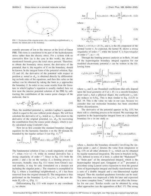
084904-3 Stress tensor on a solvated molecular surface J. Chem. Phys. 123, 084904 2005limi y,xvx − W i y,x v =0, 12→0 +S−e +s VndSxwhereW i = Gy i= 14r 2r ,i,13FIG. 1. Exclusion of the singular point y by a vanishing neighborhood o . e denotes the dotted part of the boundary.osmotic pressure of ion to the stresses at the level of linearPBE. This term is considered to be part of the hydrodynamicstress rather than the electric stress. For a system with noconvective flow as is the case in this work, the abovementionedformula gives the total stress present. Therefore,to obtain the boundary stress tensor, the derivative of thepotential, that is, the negative of E on the boundary, shouldbe known. In the integral form of the potential solution, Eqs.3 and 4, the derivative of the potential with respect toposition p, noted as ,p , is obtained directly by differentiatingon both sides of the equations, and then this value on thesurface can be obtained by taking the limit as p approachesthe boundary S. In order to use some results from the literaturein which Laplace’s equation is usually studied, here wefirst treat the interior potential solution of the PBE by subtractingthe contribution of the source point charges of themolecule, that is p = int p − 1D int q k G pk , p,k . 10kThen, the modified potential p satisfies Laplace’s equation,which is equal to the case without point charges. We will firstcalculate the derivative of p , noted as ,p , then return to thederivative of the original potential, i.e., ,p , by recoveringthe contribution from the source point charges, which is easilycalculated using Coulomb’s law.Now let us first consider the standard boundary integralequation for the harmonic function on the 3D domain ,bounded by the regular surface S see Fig. 1, 16,18lim→0 +S−e +s Gy,x x − Gy,x xdSx =0.nn11The fundamental solution G has a weak singularity of orderr −1 , when r=x−y→0, while its normal derivative has astrong singularity of order r −2 . Since in Eq. 11 both thepoints y and x lie on the surface S, a limiting process isnecessary. Actually, since Eq. 11 stems from Green’s secondidentity, it may be only formulated on a domain notincluding the singular point y. The situation is exemplified inFig. 1, where a vanishing neighborhood o of y has beenremoved from the original domain . The integration is thusperformed on the boundary S =S−e +s of the new domain =−o Fig. 1.Differentiating Eq. 11 with respect to any coordinatey i , we obtainV i =G n k x =− 1x k y i 4r 33r r,in − n i, 14where r ,i =r/x i =−r/y i , and n i is the ith component of thenormal vector n. As expected, the kernel W i shows a strongsingularity of order r −2 , while the kernel V i is hypersingularof order r −3 ,asr→0.Through the limiting process analysis as in Refs. 16 and19 the hypersingular boundary integral equation for ourmodified electrostatic potential v can be written in the followingform:c ik yv ,k y + limi y,xvx→0 +S−e V − W i y,x vxdSx + vy b iyn =0, 15where c ik and b i are bounded coefficients that only dependupon the local geometry of S at y. Ify is a smooth boundarypoint and s had a spherical shape, the coefficient c ik simplyreduces to 0.5 ik . This is then similar to Eq. 4.4.5 inRef. 19. This is the value we take in our case, because weconsider that our molecular boundary has been smoothedbefore discretization.The derivative of the potential appears in Eq. 15, butthere still is a limiting process to be treated. We rearrange theequation in the hypersingular integral form on a discretizedboundary for v in our study as12 v ,iy =−v o ,i − lim V i y,x vx→0 +s e −e n dSx+ vy b iy + lim W i y,xvxdSx,→0 +s e −e 16where s e denotes the boundary elements involving the singularpoint y, and v o ,i denotes the value from integration inEq. 15 on all other elements S−s e , which can be obtainedby regular numerical integration. The term in brackets in Eq.16, defined in terms of a limit, is called the “Hadamard” 20or “finite part” of the unregularized integral, which is thehypersingular integral part. Guiggiani et al. 16 presented aprocedure using Laurent series expansion to treat the generalform of hypersingular integral and finally transformed it intoa sum of a double integral and a one-dimensional regularintegral. Then the standard quadrature formulas can be used.The procedure was improved a little bit later and expressedin a more complete form, 17 which does not affect the formulasfor our case. Similar results can be obtained by usingother approaches see the appendixes of Ref. 17. The strongDownloaded 02 Sep 2005 to 132.239.16.167. Redistribution subject to AIP license or copyright, see http://jcp.aip.org/jcp/copyright.jsp