Systems of Linear Equations Introduction

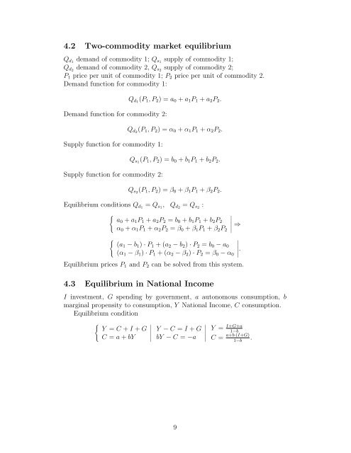
4.2 Two-commodity market equilibriumQ d1 demand of commodity 1; Q s1 supply of commodity 1;Q d2 demand of commodity 2, Q s2 supply of commodity 2;P 1 price per unit of commodity 1; P 2 price per unit of commodity 2.Demand function for commodity 1:Demand function for commodity 2:Supply function for commodity 1:Supply function for commodity 2:Q d1 (P 1 , P 2 ) = a 0 + a 1 P 1 + a 2 P 2 .Q d2 (P 1 , P 2 ) = α 0 + α 1 P 1 + α 2 P 2 .Q s1 (P 1 , P 2 ) = b 0 + b 1 P 1 + b 2 P 2 .Q s2 (P 1 , P 2 ) = β 0 + β 1 P 1 + β 2 P 2 .Equilibrium conditions Q d1 = Q s1 , Q d2 = Q s2 :{a0 + a 1 P 1 + a 2 P 2 = b 0 + b 1 P 1 + b 2 P 2α 0 + α 1 P 1 + α 2 P 2 = β 0 + β 1 P 1 + β 2 P 2∣ ∣∣∣∣⇒{(a1 − b 1 ) · P 1 + (a 2 − b 2 ) · P 2 = b 0 − a 0(α 1 − β 1 ) · P 1 + (α 2 − β 2 ) · P 2 = β 0 − α 0∣ ∣∣∣∣.Equilibrium prices P 1 and P 2 can be solved from this system.4.3 Equilibrium in National IncomeI investment, G spending by government, a autonomous consumption, bmarginal propensity to consumption, Y National Income, C consumption.Equilibrium condition{Y = C + I + GC = a + bY∣Y − C = I + GbY − C = −a∣Y = I+G+a1−bC = a+b·(I+G)1−b.9