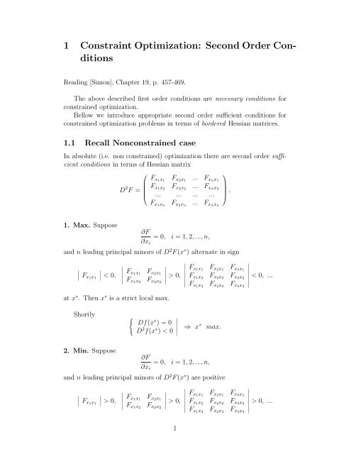
1 Constraint Optimization: Second Order Con- ditions

1 Constraint Optimization: Second Order ConditionsReading [Simon], Chapter 19, p. 457-469.The above described first order conditions are necessary conditions forconstrained optimization.Bellow we introduce appropriate second order sufficient conditions forconstrained optimization problems in terms of bordered Hessian matrices.1.1 Recall Nonconstrained caseIn absolute (i.e. non constrained) optimization there are second order sufficientconditions in terms of Hessian matrix⎛D 2 F = ⎜⎝⎞F x1 x 1F x2 x 1... F xn x 1F x1 x 2F x2 x 2... F xn x 2⎟... ... ... ...F x1 x nF x2 x n... F xnxn ⎠ .1. Max. Suppose∂F∂x i= 0, i = 1, 2, ..., n,and n leading principal minors of D 2 F (x ∗ ) alternate in sign∣ F x1 x 1∣ ∣∣ < 0,∣ ∣∣∣∣ F x1 x 1F x2 x 1F x1 x 2F x2 x 2∣ ∣∣∣∣> 0,at x ∗ . Then x ∗ is a strict local max.∣F x1 x 1F x2 x 1F x3 x 1F x1 x 2F x2 x 2F x3 x 2F x1 x 3F x2 x 3F x3 x 3∣ ∣∣∣∣∣∣< 0, ...Shortly {Df(x ∗ ) = 0D 2 f(x ∗ ) < 0∣⇒ x ∗max.2. Min. Suppose∂F∂x i= 0, i = 1, 2, ..., n,and n leading principal minors of D 2 F (x ∗ ) are positive∣ F x1 x 1∣ ∣∣ > 0,∣ ∣∣∣∣ F x1 x 1F x2 x 1F x1 x 2F x2 x 2∣ ∣∣∣∣> 0,∣F x1 x 1F x2 x 1F x3 x 1F x1 x 2F x2 x 2F x3 x 2F x1 x 3F x2 x 3F x3 x 3∣ ∣∣∣∣∣∣> 0, ...1

at x ∗ . Then x ∗ is a strict local min.Shortly {Df(x ∗ ) = 0D 2 f(x ∗ ) > 0∣⇒ x ∗min.3. Saddle. Suppose∂F∂x i= 0, i = 1, 2, ..., n,and some nonzero leading principal minors of D 2 F (x ∗ ) violate previous twosign patterns. Then x ∗ is a saddle point.1.2 Constrained Optimization of a Quadratic Form Subjectof Linear ConstraintsRecall one special case of constrained optimization, where the objective functionis a quadratic form and all constraints are linear:f(x 1 , ... , x n ) = ∑ i,ja ij x i x j ,h 1 (x 1 , ... , x n ) = ∑ ni=1 B 1i x i = 0...h m (x 1 , ... , x n ) = ∑ ni=1 B mi x i = 0.The sufficient condition in this particular case was formulated in terms ofbordered matrix⎛⎞0 ... 0 | B 11 ... B 1n... | ...0 ... 0 | B m1 ... B mn( )0 BH =− − − − − −=B 11 ... B m1 | a 11 ... a 1nB T .A⎜⎝ ... | ...⎟⎠B 1n ... B 1n | a 1n ... a nnThis (m + n) × (m + n) matrix has m + n leading principal minorsM 1 , M 2 , ... , M m , M m+1 , ... , M 2m−1 , M 2m , M 2m+1 , ... , M m+n = H.The first m matrices M 1 , ... , M m are zero matrices.Next m − 1 matrices M m+1 , ... , M 2m−1 have zero determinant.2

The determinant of the next minor M 2m is ±(det M ′ ) 2 where M ′ is theleft m × m minor of B, so det M 2m does not contain information about f.And only the determinants of last n − m matrices M 2m+1 , ... , M m+ncarry information about both, the objective function f and the constraintsh i . Exactly these minors are essential for constraint optimization.(i) If the determinant of H = M m+n has the sign (−1) n and the signs ofdeterminants of last m + n leading principal minorsM 2m+1 , ... , M m+nalternate in sign, then Q is negative definite on the constraint set Bx = 0,so x = 0 is a strict global max of Q on the constraint set Bx = 0.(ii) If the determinants of all last m + n leading principal minorsM 2m+1 , ... , M m+nhave the same sign (−1) m , then Q is positive definite on the constraint setBx = 0, so x = 0 is a strict global min of Q on the constraint set Bx = 0.(iii) If both conditions (i) and (ii) are violated by some from last m + nleading principal minorsM 2m+1 , ... , M m+nthen Q is indefinite on the constraint set Bx = 0, so x = 0 is neither maxnor min of Q on the constraint set Bx = 0.This table describes the above sign patterns:M m+m+1 M m+m+2 ... M m+n−1 M m+nnegative (−1) m+1 (−1) m+2 ... (−1) n−1 (−1) npositive (−1) m (−1) m ... (−1) m (−1) m1.3 Sufficient Condition for Constrained OptimizationConsider now the problem of maximizing f(x 1 , ..., x n ) on the constraint setC h = {x ∈ R n : h i (x) = c i , i = 1, ..., k}.As usual we consider the Lagrangiank∑L(x 1 , ..., x n , µ 1 , ..., µ k ) = f(x 1 , ..., x n ) − µ i (h i (x 1 , ..., x n ) − c i ),i=13

and the following bordered Hessian matrix⎛∂h0 ... 0 1∂h ∂x 1... 1∂x n... ... ... ... ... ...∂h 0 ... 0k∂hH =∂x 1... k∂x n∂h 1 ∂h ∂x 1... k ∂ 2 L∂x 1 ∂x 2 1⎜⎝ ... ... ... ... ... ...∂h 1 ∂h∂x n... k ∂ 2 L∂∂x n ∂x 1 ∂x n... 2 L∂x 2 n...∂ 2 L∂x n∂x 1⎞.⎟⎠This (k + n) × (k + n) matrix has k + n leading principal minorsH 1 , H 2 , ... , H k , H k+1 , ... , H 2k−1 , H 2k , H 2k+1 , ... , H k+n = H.The first m matrices H 1 , ... , H k are zero matrices.Next k − 1 matrices H k+1 , ... , H 2k−1 have zero determinant.The determinant of the next minor H 2k is ±(det H ′ ) 2 where H ′ is theupper k × k minor of H after block of zeros, so det H 2k does not containinformation about f.And only the determinants of last n − k leading principal minorsH 2k+1 , H 2k+2 , ... , H 2k+(n−k)=k+n = Hcarry information about both, the objective function f and the constraintsh i .Exactly these minors are essential for the following sufficient conditionfor constraint optimization.Theorem 1 Suppose that x ∗ = (x ∗ 1, ..., x ∗ n) ∈ R n satisfies the conditions(a) x ∗ ∈ C h ;(b) there exists µ ∗ = (µ ∗ 1, ..., µ ∗ k) ∈ R k such that (x ∗ 1, ..., x ∗ n, µ ∗ 1, ..., µ ∗ k) is acritical point of L;(c) for the bordered Hessian matrix H the last n − k leading principalminorsH 2k+1 , H 2k+2 , ... , H n+k = Hevaluated at (x ∗ 1, ..., x ∗ n, µ ∗ 1, ..., µ ∗ k) alternate in sign where the last minor H n+k =H has the sign as (−1) n .Then x ∗ is a local max in C h .If instead of (c) we have the condition(c’) For the bordered hessian H all the last n − k leading principal minorsH 2k+1 , H 2k+2 , ... , H n+k = Hevaluated at (x ∗ 1, ..., x ∗ n, µ ∗ 1, ..., µ ∗ k) have the same sign as (−1) k , then x ∗ is alocal min on C h .4

Here n = 3, k = 2 so we have to check just n − k = 3 − 2 = 1 leadingprincipal minors, so just H itself. Calculation shows that det H = 16 > 0has the sign as (−1) k = (−1) 2 = +1, so our critical point is min.Example 3. Find extremum of F (x, y) = x+y subject of h(x, y) = x 2 +y 2 =2.Solution. The lagrangian here isL(x, y) = x + y − µ(x 2 + y 2 − 2).The first order conditions give two solutionsx = 1, y = 1, µ = 0.5 and x = −1, y = −1, µ = −0.5Now it is time to switch to bordered hessian⎛⎞0 2x 2y⎜⎟H = ⎝ 2x −2µ 0 ⎠ .2y 0 −2µHere n = 2, k = 1 so we have to check just n − k = 3 − 2 = 1 leadingprincipal minor H 2 = H.Checking H for (x = 1, y = 1, µ = 0.5) we obtain H = 4 > 0, that is it hasthe sign of (−1) n = (−1) 2 , so this point is max.Checking H for (x = −1, y = −1, µ = −0.5) we obtain H = −4 < 0, thatis it has the sign of (−1) k = (−1) 1 , so this point is min.1.4 Second Order Conditions for Mixed ConstraintsProblem: maximize f(x 1 , ..., x n ) subject to k inequality and m equalityconstraintsg 1 (x 1 , ..., x n ) ≤ b 1 , ... , g k (x 1 , ..., x n ) ≤ b k ,h 1 (x 1 , ..., x n ) = c 1 , ... , h m (x 1 , ..., x n ) = c m .Lagrangian:L(x 1 , ..., x n , λ 1 , ..., λ k )) = f(x 1 , ..., x n )+−λ 1 [g 1 (x 1 , ..., x n ) − b 1 ] − ... − λ k [g ( x 1 , ..., x n ) − b 1 ]+−µ 1 [h 1 (x 1 , ..., x n ) − c 1 ] − ... − µ m [h ( x 1 , ..., x n ) − c 1 ].Theorem 2 Suppose we havex ∗ = (x ∗ 1, ..., x ∗ n), λ ∗ = (λ ∗ 1, ... , λ ∗ k), µ ∗ = (µ ∗ 1, ... , µ ∗ m)6

This formula has the following meaning:-µ ∗ j measures the sensitivity of optimal value f(x ∗ (a)) to changing theconstraint a j .-In other words µ ∗ j measures how the optimal value is affected by relaxationof j-th constraint a j .-One more interpretation: µ ∗ j measures how the additional dollar investedin j-th input changes the optimal value.That is why the Lagrange multiplier sometimes is called shadow price,internal value, marginal productivity of money.Example 4. Consider the problemMaximize f(x, y) = x 2 y on the constraint set h(x, y) = 2x 2 + y 2 = 3.The first order condition gives the solutionx ∗ (3) = 1, y ∗ (3) = 1, µ ∗ (3) = 0.5.The second order condition allows to check that this is maximizer.optimal value is f(1, 1) = 1.TheNow let us change the constraint toh(x, y) = 2x 2 + y 2 = 3.3.The first order condition gives new stationary pointx ∗ (3.3) = 1.048808848, y ∗ (3.3) = 1.048808848, µ ∗ (3.3) = 0.5244044241and the new optimal value is 1.153689733. So increasing the budget a = 3 toa + ∆a = 3.3 increases the optimal value by 1.153689733 − 1 = 0.153689733.Now estimate the same increasing of optimal value using shadow price:f(1.048808848, 1.048808848)−f(1, 1) ≈ f(1, 1)+µ ∗·0.3 = 1+0.5·0.3 = 1.15,this is good approximation of 1.153689733.1.5.1 Income Expansion PathBack to a problemMaximize f(x 1 , x 2 ) subject to h(x 1 , x 2 ) = a.The shadow price formula here looks as∂∂a f(x∗ 1(a), x ∗ 2(a)) = µ ∗ (a).8

The curve R → R n given by a → x ∗ (a) = (x ∗ 1(a), x ∗ 2(a)) is called incomeexpansion path. This is the path on which moves the optimal solution x ∗ (a)when the constraint a changes.Theorem 3 If the objective function f(x 1 , x 2 ) is homogenous, and the constraintfunction h(x 1 , x 2 ) = p 1 x 1 + p 2 x 2 is linear, then the income expansionpath is a ray from origin.Proof. Try!1.6 Envelop Theorems*The above theorems about the meaning of multiplier are particular cases ofso called Envelope Theorems.1.6.1 Version with MaximizersLet f(x, c), x ∈ R n , c ∈ R p be a function of variables x = (x 1 , ... , x n )and parameters c = (c 1 , ... , c p ). Let us fix c ∗ and suppose x ∗ (c ∗ ) be themaximizer of f(x, c ∗ ) with c ∗ fixed. Then the maximal value f(x ∗ (c ∗ ), c ∗ )can be considered as a function of c:F (c ∗ ) = f(x ∗ (c ∗ ), c ∗ ).Note that since of first order condition we haveD x f(x ∗ (c ∗ ), c ∗ ) = 0The Envelope Theorem gives an easy way to calculate the gradient of F (c ∗ ).Theorem 4D c F (c ∗ ) = D c f(x ∗ (c ∗ ), c ∗ ).Proof. By chain rule and the above mentioned first order condition we haveD c F (c ∗ ) = D x f(x ∗ (c ∗ ), c ∗ ) · D c (x ∗ (c ∗ )) + D c f(x ∗ (c ∗ ), c ∗ )= 0 · D c (x ∗ (c ∗ )) + D c f(x ∗ (c ∗ ), c ∗ ) = D c f(x ∗ (c ∗ ), c ∗ ).Example 6. Consider the maximization problemmax f(x) = −x 2 + 2ax + 4a 2which depends on the parameter a. What will be the effect of a unit increaseof a on the maximal value of f(x, a)?1. Direct solution. Just find a critical pointf ′ (x, a) = −2x + 2a = 0, x ∗ = a, F (a) = f(x ∗ (a), a) =f(a, a) = −a 2 + 2a 2 + 4a 2 = 5a 2 ,9

so the rate of change of maximal value is 10a.2. Solution using the Envelope Theorem.F ′ (a) = ∂ ∂a f(x, a)| x=a = (2x + 8a)| x=a = 10a.1.6.2 Version with Constrained MaximumConsider the problemmax f(x, a) s.t. h(x, a) = 0,depending on the parameter a. Let (x ∗ (a), µ ∗ (a)) be the optimal solution forthe fixed choice of parameter a, so F (a) = f(x ∗ (a), a) is a maximal value asa function of a.Theorem 5 The rate of change of maximal value isF ′ (a) = dda f(x∗ (a), a) = ∂ ∂a L(x∗ (a), µ ∗ (a), a).Remark. Actually when f(x, a) = f(x), that is the objective function doesnot depend on the parameter a, and h(x, a) = ¯h(x)−a, that is the parametera is the budget restriction, then we have our old result F ′ (a) = µ i , indeed,F ′ (a) = ∂ L(x, µ, a)| ∂a (x=x ∗ (a),µ=µ ∗ (a),a) =∂[f(x) − µ(¯h(x) − a)]|∂a (x=x ∗ (a),µ=µ ∗ (a),a) = µ| (µ=µ ∗ (a),a) = µ ∗ (a).Example 7. Consider the problem discussed abovemax f(x, y) = x 2 y s.t. h(x, y) = 2x 2 + y 2 = 3.As it was calculated the first order condition gives the solutionx ∗ (3) = 1, y ∗ (3) = 1, µ ∗ (3) = 0.5,the second order condition allows to check that this is maximizer. The optimalvalue is f(1, 1) = 1.Now try to estimate how the optimal value will change if we replace theconstraint byh(x, y) = 2x 2 + 1.1y 2 = 3.Instead of solving the problemmax f(x, y) = x 2 y s.t. h(x, y) = 2x 2 + 1.1y 2 − 3 = 0let us use the Envelope Theorem forh(x, y, a) = 2x 2 + ay 2 − 3.10

The Lagrangian in this case isthenthusL(x, y, a) = x 2 y − µ(2x 2 + ay 2 − 3),F ′ (a) = dda L(x, y, a) = −µy2 ,F ′ (1) = dda L(x, y, a)| (x=1,y=1,µ=0.5) = −µy 2 | (x=1,y=1,µ=0.5) = −0.5 · 1 2 = −0.5,andF (1.1) = F (1) + F ′ (1) · 0.1 = 1 + (−0.5) · 0.1 = 1 − 0.05 = 0.95.11

Exercises1. Write out the bordered Hessian for a constrained optimization problemwith four choice variables and two constraints. Then state specifically thesecond-order sufficient condition for a maximum and for a minimum respectively.2. For the following problems(i) find stationary values,(ii) ascertain whether they are min or max,(iii) find whether relaxation of the constraint (say increasing of budget) willincrease or decrease the optimal value?(iv) At what rate?(a) f(x, y) = xy, h(x, y) = x + 2y = 2;(b) f(x, y) = x(y + 4), h(x, y) = x + y = 8;(c) f(x, y) = x − 3y − xy, h(x, y) = x + y = 6;(d) f(x, y) = 7 − y + x 2 , h(x, y) = x + y = 0.3. Find all the stationary points of f(x, y, z) = x 2 y 2 subject of x 2 +y 2 = 2and check the second order conditions.4. Find all the stationary points of f(x, y, z) = x 2 y 2 z 2 subject of x 2 +y 2 + z 2 = 3 and check the second order conditions.5. Find the maximum and minimum values of f(x, y) = x 2 + y 2 on theconstraint set h(x, y) = x 2 + xy + y 2 = 3. Redo the problem, this time usingthe constraint h(x, y) = 3.3.Now estimate the shadow price of increasing of constraint by 0.3 unitsand compare with previous result.∗ And now estimate the change of optimal value when the objective functionis changed to f(x, y) = x 2 + 1.2y 2 keeping h = x 2 + xy + y 2 = 3.6. Find all the stationary points of f(x, y, z) = x + y + z 2 subject tox 2 + y 2 + z 2 = 1 and y = 0. Check the second order conditions and classifyminimums and maximums.Homework1. Exercise 1.2. Exercise 2d.3. Exercise 4.4. Exercise 6.5. Exercise 19.3 from [Simon].12