small satellite attitude control based on a kalman filter

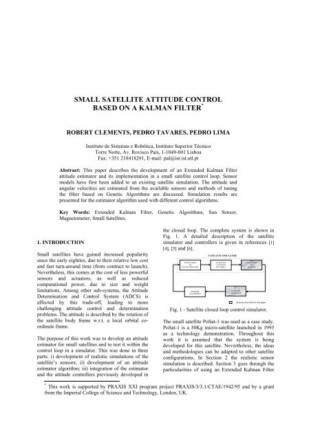
SMALL SATELLITE ATTITUDE CONTROLBASED ON A KALMAN FILTER *ROBERT CLEMENTS, PEDRO TAVARES, PEDRO LIMAInstituto de Sistemas e Robótica, Instituto Superior TécnicoTorre Norte, Av. Rovisco Pais, 1-1049-001 LisboaFax: +351 218418291, E-mail: pal@isr.ist.utl.ptAbstract: This paper describes the development of an Extended Kalman Filter<strong>attitude</strong> estimator and its implementation in a <strong>small</strong> <strong>satellite</strong> <strong>control</strong> loop. Sensormodels have first been added to an existing <strong>satellite</strong> simulation. The <strong>attitude</strong> andangular velocities are estimated from the available sensors and methods of tuningthe filter <strong>based</strong> on Genetic Algorithms are discussed. Simulation results arepresented for the estimator algorithm used with different <strong>control</strong> algorithms.Key Words: Extended Kalman Filter, Genetic Algorithms, Sun Sensor,Magnetometer, Small Satellites.1. INTRODUCTIONSmall <strong>satellite</strong>s have gained increased popularitysince the early eighties, due to their relative low costand fast turn-around time (from contract to launch).Nevertheless, this comes at the cost of less powerfulsensors and actuators, as well as reducedcomputational power, due to size and weightlimitations. Among other sub-systems, the AttitudeDetermination and Control System (ADCS) isaffected by this trade-off, leading to morechallenging <strong>attitude</strong> <strong>control</strong> and determinationproblems. The <strong>attitude</strong> is described by the rotation ofthe <strong>satellite</strong> body frame w.r.t. a local orbital coordinateframe.The purpose of this work was to develop an <strong>attitude</strong>estimator for <strong>small</strong> <strong>satellite</strong>s and to test it within the<strong>control</strong> loop in a simulator. This was done in threeparts: i) development of realistic simulations of the<strong>satellite</strong>’s sensors; ii) development of an <strong>attitude</strong>estimator algorithm; iii) integration of the estimatorand the <strong>attitude</strong> <strong>control</strong>lers previously developed inthe closed loop. The complete system is shown inFig. 1. A detailed description of the <strong>satellite</strong>simulator and <strong>control</strong>lers is given in references [1][4], [5] and [6].SIMULATIONOFMAGNETORQUERSCONTROLALGORITHMSATELLITE SIMULATORSATELLITEATTITUDEDYNAMICSATTITUDEESTIMATORSIMULATIONOFSENSORSSystems described in this paper.Fig. 1 - Satellite closed loop <strong>control</strong> simulator.The <strong>small</strong> <strong>satellite</strong> PoSat-1 was used as a case study.PoSat-1 is a 50Kg micro-<strong>satellite</strong> launched in 1993as a technology demonstration. Throughout thiswork it is assumed that the system is beingdeveloped for this <strong>satellite</strong>. Nevertheless, the ideasand methodologies can be adapted to other <strong>satellite</strong>configurations. In Section 2 the realistic sensorsimulation is described. Section 3 goes through theparticularities of using an Extended Kalman Filter* This work is supported by PRAXIS XXI program project PRAXIS/3/3.1/CTAE/1942/95 and by a grantfrom the Imperial College of Science and Technology, London, UK.

for <strong>attitude</strong> estimation. The filter tuning <strong>based</strong> onGenetic Algorithms is covered in Section 4. Theresults of closed loop <strong>attitude</strong> <strong>control</strong> with andwithout the estimator for three different <strong>control</strong>algorithms are discussed in Section 5. The paperends with conclusions and prospects for future work,in Section 6.and the vector to the Sun is less than the angle of theradius of the Earth as seen from the <strong>satellite</strong>. Theangle of the radius of the Earth is pre-calculatedwithin the simulator from the orbit altitude, so canbe considered known at all time.2. SENSOR SIMULATIONTwo PoSat-1 sensors are available for <strong>attitude</strong>estimation: the magnetometer and the sun sensor.The magnetometer measures the geomagnetic fieldvector and the <strong>attitude</strong> is determined by comparingthis vector with the expected geomagnetic field atthe current orbital location, <strong>based</strong> on the widely usedIGRF model [8]. Therefore, the sensor reading canbe simulated by rotating the current geomagneticfield vector into the <strong>satellite</strong> co-ordinate system(SCS) [5].The Sun sensor measures the relative Sun and<strong>satellite</strong> locations from the angle of incidence of thesunlight on the sensor. From the knowledge of theSun and spacecraft orbital locations, the current andexpected measurements can be compared todetermine the <strong>attitude</strong>. PoSat-1 has two Sun sensorswith each sensor having two channels. Both sensor’sfield of view lie in the x-y plane, one looking in thepositive y-direction, the other in the negativex-direction (in SCS).A number of common Sun sensor designs are givenin [8]. PoSat-1 Sun sensors layout is that shown inFig. 2. Each sensor consists of two light sensitivecells, therefore producing the two-channel output.Each cell is angled to the horizontal as shown in thefigure. To implement this design it is necessary todetermine the geometry of the sensor (i.e. angles αand β). Two key characteristics in the telemetry datafrom PoSat-1 allow these angles to be determined.These are that both channels of the sensor startreading at the same time and that one channel startsreading at a non-zero, positive value. The <strong>satellite</strong>technical documentation also states that the field ofview should be ±60 0 . To satisfy these requirementsα=β=30 o . This design is just shown in twodimensions. In three dimensions the surroundingstructure would provide a similar ±60 o view limit.Field of View Limited providedby Surrounding StructureLight Sensitive CellsαFig. 2 - Sun Sensor DesignThe simulator must also consider the possibility ofthe Earth being between the <strong>satellite</strong> and the Sun.This case is simply detected by calculating if theangle between the vector to the centre of the EarthβField of View LimitFig. 3 - Comparison of Telemetry and simulationIt is clear from the telemetry that the value of outputfrom the sensors when they can’t see the Sun varies.Initial thought might suggest that the off value of thesensor should always be zero. However, it wasrealised that this variation was due to the sensorpicking up sunlight reflected from the Earth. So, ifthe <strong>satellite</strong> is over the dark side of the Earth, the offvalue will be zero, if it is over the lit side it will havea slightly increased value. The magnitude of thisincrease will depend on factors like weatherconditions, current altitude and whether the <strong>satellite</strong>is over land or sea. The ‘off’ value over the lit sideof the Earth has thus been modelled using a randomnoise signal which gives values similar to those seenin the telemetry.Fig. 4 - Comparison of Telemetry and SimulationComparison of the output from the simulator withtelemetry data from PoSat-1 can be seen in Fig. 3and 4. Figure 3 shows a comparison for one orbit(showing just one channel). It can be seen that realand simulated data are very similar. The differencesin number and magnitude of each peak are due todifferences in <strong>attitude</strong> and spin rate of the <strong>satellite</strong> inthe simulation and in reality. The <strong>attitude</strong> of PoSat-1is not known exactly so it is not possible to get thesimulator to have exactly the same results. Themodelling of the off-value can also be seen in thisfigure. Figure 4 shows the comparison of one- -

4. ESTIMATOR TUNINGThere are three matrices used within the estimatorthat must be determined before it can be used. Theseare P o (7x7) – the covariance of the error in the initialstate, Q (7x7) – the covariance of the system modelerror, and R (3x3 or 6x6) 1 – the covariance of themeasurement error. We have chosen to tune thesecovariance matrices instead of making them matchsensor noise characteristics, so as to improve closedloop <strong>control</strong> performance.Initially it would seem that there are 77 parameterswhich need to be determined (noting that covariancematrices are always symmetric). To simplify theproblem, various parameters within each matrix canbe grouped by assuming that the error covariance inthe terms will be the same. For example, it isreasonable to assume that the covariance of theerrors in the Ω x and Ω y terms will be the same. TheΩ z term may to different because it involves the spinof the <strong>satellite</strong>.This grouping can reduce the total number ofparameters to 32. The P matrix can be tunedseparately from Q and R because P only effects theinitial transient errors. Q and R can be tunedignoring transient effects, therefore reducing theproblem further.Because of the multi-parameter, non-linear, multiminimumnature of this optimisation problem alogical approach was to use a genetic algorithm(GA) [3]. A standard GA has been used, withchromosomes containing all the elements of theestimator covariance matrices. Each population wasevaluated by simulating each chromosome over anumber of orbits and evaluating a cost functioncontaining the average estimator error. Newpopulations were generated using mutations andcrossover with parents being selected using aroulette wheel selection process. This is a veryeffective method of tuning the estimator although,due to simulation time, it can be very slow.Table 1 - Estimator Accuracy ResultsMeanStandardDeviationWorstPointingError (deg)0.58 0.56 1.72Spin RateError, %0.39 0.37 1.23The best average estimator results, shown in Table1, were obtained in closed loop using a predictive<strong>control</strong>ler, described in the following section, over anumber of orbits. These results were obtained over1 The R matrix size changes depending on whetherthe Sun sensor is included or not.twenty simulations each ten orbits long withdifferent starting conditions.5. CLOSED LOOP CONTROLThere are three <strong>control</strong>lers of interest that areavailable within the simulator: the Predictive<strong>control</strong>ler [4], the Energy <strong>control</strong>ler [9] and theAlpha-Beta <strong>control</strong>ler [7]. The predictive <strong>control</strong>lerattempts to predict, for all possible actuations, thechange in angular velocity of the <strong>satellite</strong> if thatactuation was applied. It then determines which ofthese will cause the greatest reduction in the<strong>satellite</strong>’s kinetic energy. As a result, a time-varying<strong>control</strong> law is applied. The energy <strong>control</strong>ler uses the<strong>control</strong> lawcccm( t)= h Ω ( t)× B(t), (8)cowhere h is a positive constant. The alpha-beta<strong>control</strong>ler is the <strong>control</strong>ler currently used on PoSat-1. It uses the <strong>control</strong> lawcm z⎛ dβdα⎞= k⎜− ⎟ , (9)⎝ dt dt ⎠where α is the angle between the z-axis of the OCSand the expected geomagnetic field and β is theangle between the z-axis of the OCS and themeasured geomagnetic field. The alpha-beta<strong>control</strong>ler does not require an estimator. Both thePredictive <strong>control</strong>ler and the Energy <strong>control</strong>ler can<strong>control</strong> the spin of the <strong>satellite</strong> as well as the <strong>attitude</strong>,while the alpha-beta <strong>control</strong>ler only <strong>control</strong>s <strong>attitude</strong>.These <strong>control</strong>lers are described and theirperformance without an estimator compared in detailin [5].To compare the effectiveness of the <strong>control</strong>lers andestimator in the loop, twenty simulations, each tenorbits in duration with varying starting conditions,were made. The results presented below are averageresults from these tests, where spin <strong>control</strong> as well as<strong>attitude</strong> stabilisation were envisaged. Since thealpha-beta <strong>control</strong>ler can not <strong>control</strong> spin, a differenttest with no spin <strong>control</strong> required was used to makecomparisons with this <strong>control</strong>ler.To check the effect of the estimator on the energyand predictive <strong>control</strong>lers, tests were first conductedwithout the estimator. Table 2 shows results for thepredictive and energy <strong>control</strong>lers.Table 2 – Simulation Results without EstimatorSettlingTime to 5 o(orbits)PointingAccuracy(deg)Spin RateAccuracy(rad/s)Energy(Joules)PredictiveController2.40 1.86 4.6x10 -5 2.70x10 5EnergyController2.75 1.85 8.8x10 -4 2.56x10 5- -

Comparing the performance of the two <strong>control</strong>lerswithout the estimator, both have very similar results.Considering the standard deviations of theseaverages (not shown here) the slight differences areinsignificant. This is true with the exception of thespin rate accuracy where the predictive <strong>control</strong>ler isconsiderably better.Table 3 – Simulation Results with EstimatorPredictiveController(without SunSensor)PredictiveController(with SunSensor)EnergyController(with SunSensor)SettlingTime to 5 o(orbits)PointingAccuracy(deg)Spin RateAccuracy(rad/s)Energy(Joules)8.76 3.22 1.3x10 -4 3.84x10 59.18 3.14 1.2x10 -4 4.09x10 52.74 2.04 6.5x10 -4 2.70x10 5Table 3 shows the results for the two <strong>control</strong>lerswith the estimator included. This table also showsthe results for the estimate with and without the sunsensor, for the predictive <strong>control</strong>ler.Looking at the effect of the estimator on thepredictive <strong>control</strong>ler, the pointing accuracy hasdeteriorated from ≈1.8 o to ≈3.2 o . Similarly, the spinrate accuracy has been halved. The energyconsumed has also increased slightly. Consideringthe effect of the estimator on the energy <strong>control</strong>ler,the reduction in accuracy is much <strong>small</strong>er. Pointingaccuracy is reduced from ≈1.8 o to ≈2.0 o . Spin rateand energy consumed are not significantly affected.Thus, comparing the <strong>control</strong>ler + estimatoralgorithms, the energy <strong>control</strong>ler is better frompointing accuracy, rapid settling and energystandpoints. However, the predictive <strong>control</strong>ler stillhas a better spin rate accuracy.Table 4 – Comparisons to Alpha-Beta ControllerAlpha-BetaControllerPredictiveControllerEnergyControllerTuned PredictiveControllerSettlingTime to 1 o(orbits)PointingAccuracy(deg)EnergyConsumed(Joules)No Settling 1.26 3.20x10 34.00 0.14 1.66x10 50.80 0.01 2.51x10 51.80 0.02 7.67x10 3For a <strong>control</strong>ler + estimator algorithm to be usedwith PoSat-1, it must perform better than its currentalpha-beta <strong>control</strong>ler. In Table 4, results of thealpha-beta, predictive and energy <strong>control</strong>lers arecompared with no estimator in the loop and no spin<strong>control</strong>. The alpha-beta <strong>control</strong>ler does not requirean estimator and can not <strong>control</strong> spin, hence thethree <strong>control</strong> algorithms were compared under thesame circumstances.The energy <strong>control</strong>ler clearly has the best pointingaccuracy and settling time. However, the energyconsumed is considerably larger than that used bythe alpha-beta <strong>control</strong>ler. The predictive <strong>control</strong>leroutperforms the alpha-beta <strong>control</strong>ler regardingpointing accuracy and settling time, but energyconsumption is high too. This shows that, to useeither the predictive or the energy <strong>control</strong>ler theirenergy consumption must be reduced. Both thepredictive <strong>control</strong>ler and the energy <strong>control</strong>lercontain a number of parameters that can be adjustedto change their performance. To improve the overall<strong>control</strong>ler + estimator performance, the estimatorand the <strong>control</strong>ler parameters can be tuned togetherin closed loop. Only limited exploration of this sortof tuning has been possible during this work, but thelast row of Table 4 shows results that were obtainedafter the predictive <strong>control</strong>ler was tuned to reduceenergy consumption. Comparing these to the alphabeta<strong>control</strong>ler results, the <strong>control</strong>ler now usessimilar energy but with a pointing accuracy about 50times better. It is also noticeable that these accuracyresults are better than the pre-tuning <strong>control</strong>lerresults. Furthermore, it should be noted that theenergy <strong>control</strong>ler was tested with unrestrictedactuators, while the predictive <strong>control</strong>ler usesrestricted actuators. Nonetheless, their performanceunder such distinct conditions is similar. Usually, theenergy <strong>control</strong>ler produces bad results withrestricted actuators.6. CONCLUSIONS AND FUTURE WORKA Kalman Filter <strong>attitude</strong> estimator usingmagnetometers and sun sensors has been developedand implemented showing, in realistic simulations, apointing accuracy of ≈0.6 o and a spin rate error of≈0.4%. A genetic algorithm has been used to tunethe Kalman filter estimator. With the estimator inthe loop the system worked best with the energy<strong>control</strong>ler where there was an accuracy loss of only0.2 degrees. With the predictive <strong>control</strong>ler the dropin performance was nearly 1.4 degrees. The obtainedresults suggest that these <strong>control</strong>lers outperform thebenchmark alpha-beta <strong>control</strong>ler regarding accuracy.Further work on closed loop tuning could reapsignificant rewards. It has been shown that tuningthe <strong>control</strong>lers can make major improvements inareas like energy consumption and pointingaccuracy. Another important area not considered sofar is the processing time required by the estimatorand <strong>control</strong>ler. On a <strong>small</strong> <strong>satellite</strong> it is important tominimise the computation effort that is required to<strong>control</strong> the <strong>attitude</strong>. Currently the predictive andenergy <strong>control</strong>lers with the estimator use about threetimes more CPU time than the alpha-beta <strong>control</strong>ler.One potential method to reduce the computationeffort associated to the estimation would be to- -

linearise the equations of motion about a number ofkey <strong>attitude</strong>s and then use a gain scheduling<strong>control</strong>ler to determine the motion between theselinearised points. At the moment the equations arelinearised at every time step, a time consumingprocess. In a real <strong>satellite</strong>, the <strong>attitude</strong> perturbationfrom the stabilised position will be <strong>small</strong>, and so few<strong>attitude</strong> way-points would be required to achieveaccurate results.REFERENCES[1] Bak, T., Blanke, B., Wisniewsky, R., Astolfi, A.,Spindler, K., Tavares, P., Tabuada, P., Lima, P. (2000),"Satellite Attitude Control Problem", in COSY Book,Springer-Verlag.[2] Bar-Itzhack, I.Y., Oshman, Y. (1985), "AttitudeDetermination from Vector Observations: QuaternionEstimation", IEEE Transaction on Aerospace andElectronic Systems, Vol.21, No.1, pp 128-135.[3] Goldberg, D. (1989), Genetic Algorithms in Search:Optimisation and Machine Learning, Addison-Wesley.[4] Tabuada, P., Alves, P., Tavares, P., Lima, P. (1999) "APredictive Algorithm for Attitude Stabilisation and SpinControl of Small Satellites", Proc. of the EuropeanControl Conference (ECC’99), Karlsruhe, Germany.[5] Tabuada, P., Alves, P., Tavares, P., Lima, P. (1998),Attitude Control Strategies for Small Satellites, Institutefor Systems and Robotics internal report RT-404-98.[6] Tavares, P., Sousa, B., Lima, P. (1998), "A Simulatorof Satellite Attitude Dynamics", Proc. of the 3 rdPortuguese Conference on Automatic Control, Vol. II, pp.459-464, Coimbra, Portugal.[7] Ong, W. T. (1992), Attitude Determination andControl of Low Earth Orbit Satellites, MSc Thesis, Dept.of Electric and Electrical Engineering, University ofSurrey, U.K.[8] Wertz, J.R. (1990), Spacecraft Attitude Determinationand Control, Kluwer Academic Publishers.[9] Wisniewski, R. (1996), Satellite Attitude Control usingonly Electromagnetic Actuation, Ph.D. Thesis, Dept. ofControl Engineering, Aalborg University, DanmarkAPPENDIX AExtended Kalman Filter Algorithm [2]1) Calculation of Kalman GainT−[ H P H ] 1TKk + 1= Pk+ 1 / kHk + 1 / k k + 1 / k k + 1 / k k + 1 / k+ R (10)where K k+1 is the Kalman Gain Matrix (7x3), P k+1/k isthe perturbation covariance matrix (7x7) at time k+1given the measurements at time k, R is themeasurement error covariance matrix (3x3) andH k+1/k is a (3x7) matrix defined as follows:[ h h h ]Hk + 1 / k= 03x31 2 3h4(11)dD(qˆk)where hi= borb,k + 1, q ˆikdqˆ,is the i th estimatedi,kcomponent of quaternion q at time k and b orb,k+1 isthe model magnetic field vector (in OCS) at timek+1.2) Update the Stated z K ( b − D b ) (12)ˆk+ 1 / k + 1=k + 1 meas,k + 1×orb,k + 1ˆ ˆ ˆk + 1 / k + 1= zk+ 1 / k+ dzk+ 1 / k + 1z (13)z ˆ + /wherek 1 kis the estimated state vector at timek+1 given the measurements at k,x y zz = [ Ω] TsiΩsiΩsiq1q2q3q4b meas,k+1 is the measurement magnetic field vector (inxSCS) at time k+1, Ωsiis the x component of theangular velocity in SCS w.r.t. ICS and D is therotation matrix from OCS to SCS as defined below:2 2 2 2⎡qˆ− ˆ − ˆ + ˆ+− ⎤1, 2, 3, 4,2(ˆ ˆ ˆ ˆˆ ˆ ˆ1, 2, 3, 4,) 2( ˆkqkqkqkqkqkqkqkq1,kq3,kq2,kq4,k ) (14)⎢D = ⎢ 2(ˆ q ˆ − ˆ ˆ1, kq2,kq3,kq4,k)⎢⎣2(ˆ q ˆ1, 3,+ ˆ ˆkqkq2,kq4,k )2−qˆ1,+ ˆkq2(ˆ q qˆ2, k22, k3, k2 2−qˆ3,+ ˆkq4,−qˆqˆ)1, k4, kk2(ˆ q ˆ2, kq2 2−qˆ−qˆ1, k3, k2, k⎥+ qˆˆ1, kq4,k) ⎥2 2+ qˆ+ ˆ ⎥3, kq4,k ⎦3) Update the Covariance MatrixThe perturbation covariance matrix is updated using(16) where H k+1/k+1 is calculated from (12) exceptthat the quaternions at time k+1 are used instead ofat time k.T T[ I −KH ] P [ I −KH ] K RKPk+ 1 / k+1 (7x7) k+1 k+1/ k+1 k+1/ k (7x7) k+1 k+1/ k+1+k+1 k+1= (15)4) Propagate State Vectork + 2z ˆ2 / 11( ˆˆk + k + =∫fk+zk+ 1 / k + 1,k + 1) dt + z (16)k + 1 / k + 1k + 1⎡ Ω ⎤wheresif+zˆk 1(k + 1/ k + 1,k + 1) = ⎢ ⎥ ,⎣ q⎦q = Ωq , and Ω si= I [ ngg+ nctrl− Ωsi× ( IΩsi)]−1(n ctrl is the <strong>control</strong> moments vector).2n [ ] Tgg= 3ωo( Ix− Iz) D33− D23D130zy x⎡ 0 Ω⎤so− ΩsoΩso⎢ zx y ⎥1 ⎢−Ωso0 ΩsoΩsoΩ =⎥2 ⎢ yxzΩ − 0 ⎥soΩsoΩso⎢⎥x y z⎢⎣− Ωso− Ωso− Ωso0 ⎥⎦xD ij is an element of D and Ωsois the x component ofangular velocity in SCS w.r.t. OCS.5) Propagate the Perturbation Covariance MatrixTPk + 2 / k + 1= Φk + 2 / k + 1Pk+ 1 / k + 1Φk + 2 / k + 1+ Q , (17)where Q is the system error covariance matrix,Φ I + F zˆ, k 1)∆tk + 2 / k + 1=(7 x7)(k + 1 / k + 1+ ,⎡δΩ⎤siF( zˆk + 1 / k + 1,k + 1) δz= ⎢ ⎥ ,⎣ δq⎦δ Ω = I−1 δn− δΩ× IΩ− Ω × IδΩ,siδn gg[ ]ggis given byδngg= 6ωo ( I x− I z).⎡−Dˆ33qˆ4+ Dˆ23qˆ1⎢. ⎢ Dˆ33qˆ3− Dˆ13qˆ1⎢⎣− Dˆ33qˆ3+ Dˆ23qˆ2− Dˆ33qˆ4− Dˆ13qˆ2sisi2(18)− Dˆ33qˆ2− Dˆ23qˆ3Dˆ33qˆ1+ Dˆ13qˆ3sisi− Dˆ33qˆ1− Dˆ23qˆ4 ⎤⎥− Dˆ33qˆ2+ Dˆ13qˆ4⎥δq⎥⎦⎡ qˆ4− qˆ3qˆ2 ⎤⎢⎥1δ q = Ωsiδq+ βδΩsi, ⎢qˆ3qˆ4− qˆ1β =⎥ .2 ⎢−qˆˆ ˆ ⎥2q1q4⎢⎥⎣−qˆ1− qˆ2− qˆ3 ⎦- -