An Introduction to the Conjugate Gradient Method Without the ...

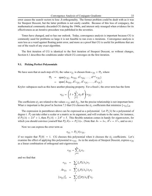
££§¢¡¡¡0¡¢¡¥ £¥ £¡§2£ ¥£2 ¢0¡¥2 £ ¦¦¦¦¦¦¦¦¦¤£¥¢¥¥3 ¢0¡ ¥¡ ¦ ¨ ¦¡ ¦ ¨ ¡ ¦ ¦¡ ¦ ¨1 £¢¢Convergence Analysis of Conjugate Gradients 33error causes the search vectors to lose -orthogonality. The former problem could be dealt with as it wasfor Steepest Descent, but the latter problem is not easily curable. Because of this loss of conjugacy, themathematical community discarded CG during the 1960s, and interest only resurged when evidence for itseffectiveness as an iterative procedure was published in the seventies.Times have changed, and so has our outlook. Today, convergence analysis is important because CG iscommonly used for problems so large it is not feasible to run even § iterations. Convergence analysis isseen less as a ward against floating point error, and more as a proof that CG is useful for problems that areout of the reach of any exact algorithm.The first iteration of CG is identical to the first iteration of Steepest Descent, so without changes,Section 6.1 describes the conditions under which CG converges on the first iteration.9.1. Picking Perfect PolynomialsWe have seen that at each step of CG, the value ¢, wherespan¡ £¡ is chosen from ¢0¡span¡ ¢0¡¢0¡ 0¡Krylov subspaces such as this have another pleasing property. For ¥ a fixed , the error term has the form0¡ 0¡£¡0¡The coefficients¢¦are related to the values¡ , but the precise relationship is not important here.What is important is the proof in Section 7.3 that CG chooses ¤ ¦coefficients that minimize § ¢¡§.the¢¦¡ and ¡ 1¢¢¥ ¦¢Let¦ ¡ ¨¥¥.¦if¦¡2¥¨ ¨¢£then¦£2¥¡ £The expression in parentheses above can be expressed as a polynomial. be a polynomial ofdegree can take either a scalar or a matrix as its argument, and will evaluate to the same; for instance,221, 2 2 . This flexible notation comes in handy for eigenvectors, for,2. (Note that2, and so on.)which you should convince yourself that¦¥¨ £¦¥¡ ¨£ ¡Now we can express the error term as¨if we require that¦¥ 0¨ £ 1. CG chooses this polynomial when it chooses the¢¦0¡coefficients. Let’s¢£¦examine the effect of applying this polynomial ¢ 0¡ to . As in the analysis of Steepest Descent, ¢ expressas a linear combination of orthogonal unit eigenvectors0¡¦ ¦0¡¤ ¥ £ ¦and we find that1¦¢¢2 ¦¦¦¦2 ¡ ¦