An Introduction to the Conjugate Gradient Method Without the ...

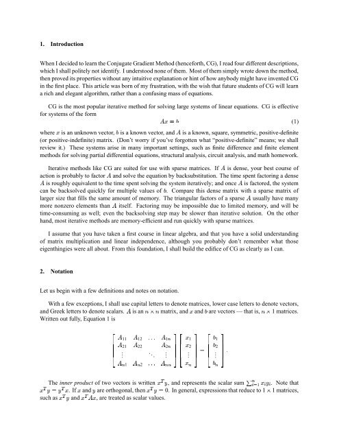
¢£©§¢£¡¡¡¤©§£¢£¥¥¥¤©§1. IntroductionWhen I decided to learn the Conjugate Gradient Method (henceforth, CG), I read four different descriptions,which I shall politely not identify. I understood none of them. Most of them simply wrote down the method,then proved its properties without any intuitive explanation or hint of how anybody might have invented CGin the first place. This article was born of my frustration, with the wish that future students of CG will learna rich and elegant algorithm, rather than a confusing mass of equations.CG is the most popular iterative method for solving large systems of linear equations. CG is effectivefor systems of the form¢¡ £ ¥where ¡ is an unknown vector, ¥ is a known vector, andis a known, square, symmetric, positive-definite(or positive-indefinite) matrix. (Don’t worry if you’ve forgotten what “positive-definite” means; we shallreview it.) These systems arise in many important settings, such as finite difference and finite elementmethods for solving partial differential equations, structural analysis, circuit analysis, and math homework.Iterative methods like CG are suited for use with sparse matrices. If is dense, your best course ofaction is probably to factor and solve the equation by backsubstitution. The time spent factoring a denseis roughly equivalent to the time spent solving the system iteratively; and once is factored, the systemcan be backsolved quickly for multiple values of . Compare this dense matrix with a sparse matrix oflarger size that fills the same amount of memory. The triangular factors of a sparse usually have manymore nonzero elements than itself. Factoring may be impossible due to limited memory, and will betime-consuming as well; even the backsolving step may be slower than iterative solution. On the other¥hand, most iterative methods are memory-efficient and run quickly with sparse matrices.I assume that you have taken a first course in linear algebra, and that you have a solid understandingof matrix multiplication and linear independence, although you probably don’t remember what thoseeigenthingies were all about. From this foundation, I shall build the edifice of CG as clearly as I can.(1)2. NotationLet us begin with a few definitions and notes on notation.With a few exceptions, I shall use capital letters to denote matrices, lower case letters to denote vectors,1 matrices.Written out fully, Equation 1 isand Greek letters to denote scalars. is an § § matrix, and ¡ and ¥ are vectors — that is, §¢¡¢¢11 1¤1221 2¤22.. .. .¦¨§ §§¢¡¢¢12.¦¨§ §§¢¡¢¢12.¦¨§ §§¤ 1 ¤ 2 ¤¥¤The inner product of two vectors is written , and represents the scalar sum ¡ £ ¡ ¡¤1 . Note that¡. If ¡ and are orthogonal, then ¡ £ 0. In general, expressions that reduce to 1 1 matrices,such as ¡ and ¡ ¡ , are treated as scalar values.