Improved Models for Graceful Graphs

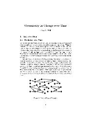
A possible set of constraints to eliminate the graph symmetry is x 1 < x 2 , x 2 < x 3 , toexclude permutations within the cliques and x 1 < x 4 , x 1 < x 5 , x 1 < x 6 to excludeswapping the cliques and permuting both. Since the constraints imply that x 1 = 0, thisconstraint together with x 2 < x 3 is sufficient.We have shown in [13] that combinations of value symmetries with variable symmetriescould be broken by a combination of lexicographic ordering constraints andelement constraints. We state one such constraint for each combination of the complementsymmetry with one variable symmetry.The model just described, which will be called the node model in the rest of thepaper, is adequate to find all graceful labellings of the graph in Figure 1, and allowed usto investigate slightly larger graphs as well, e.g. the related graphs K 4 × P 2 , K 5 × P 2 ,and K 6 × P 2 . K 5 × P 2 is graceful, and has a unique graceful labelling, apart fromsymmetric equivalents, whereas K 6 × P 2 is not graceful; these new results are nowlisted in Gallian’s survey [4]. Results that we obtained with this model for other classesof graph are summarized in [16]. However, the search effort and run time increaserapidly with problem size, so that it is very time-consuming, as shown below, to provethat K 7 ×P 2 , with 14 nodes and 49 edges, is not graceful; K 8 ×P 2 is out of reach withina reasonable time. In the next sections, a better model of the problem is introduced.3 The Edge-Label ModelA more efficient model has been recently introduced in [17]. We summarize it here. Itsroots are in a search algorithm by Beutner & Harborth [2]. They use a backtrackingsearch procedure, based on the approach in the proof, to find graceful labellings orprove that there are none. They focus on the edge labels, considering each label inturn, from q (the number of edges) downwards. Each edge label has to be used, andappear somewhere in the graph, and they construct a labelling, or prove that there is nolabelling, by trying to decide, for each edge label in turn, which node labels will appearat either end of the edge. The classes they consider are nearly complete graphs, withspecific kinds of sub graph removed from a clique; for instance, they show that K n − e,i.e. an n-clique with one edge removed, is graceful only for n ≤ 5 and that any graphderived from K n by removing 2 or 3 edges is not graceful for n > 6.The edge-label model has a variable e i for each edge label i, which indicates howthis edge label will be formed. The value assigned to e i is the smaller node label formingthe edge labelled i, i.e. if e i = j, the edge labelled i joins the nodes labelled j and j + i.Hence, the domain of e i is {0, 1, ..., q −i}. (Essentially, an edge label is associated witha pair of node labels, but since if the edge label and the smaller node label are known,the other node label is also known, we need only associate an edge label with onenode label.) Note that the domain of e q is {0}. The domain of e q−1 is initially {0, 1}but this can be reduced either to {1} or to {0} arbitrarily, to break the complementsymmetry. We choose to set e q−1 = 1 (although choosing e q−1 = 0 instead makeslittle difference).There is also a variable l j for each node label j; the value of l j represents the node towhich the label j is attached, provided that this node label is used at all in the labelling.To allow for the fact that a label may not be used, the domains of these variables contain

a dummy value, say n+1. The node label variables must all have different values (unlessthey are assigned the dummy value).The link between the two sets of variables is achieved by the constraints: e i = j iffthe values of l j and l j+i represent adjacent nodes in the graph (1 ≤ i ≤ q; 0 ≤ j ≤q − i). In Solver 6.3, this is expressed as a table constraint, using a ternary predicatewhich uses the adjacency matrix of the graph. GAC is enforced on table constraints,which is relatively slow.The graph symmetry, if any, has still to be dealt with. In the edge-label model, itappears as value symmetries affecting the node-label variables. If a graph symmetryσ maps the node numbered i to the node numbered σ(i), then it maps the assignmentl j = i to the assignment l j = σ(i), whereas in the node model, it maps x i = j intox σ(i) = j. Law and Lee [8] point out that value symmetry can be transformed intovariable symmetry acting on the dual variables and then is amenable to the Crawford etal. procedure for deriving symmetry-breaking constraints.Hence, a simple way to derive symmetry-breaking constraints in the edge-labelmodel is to re-introduce the variables x 1 , ..., x n from the node model. These are theduals of the node label variables l 1 , ..., l q . The two sets of variables can be linked by thechannelling constraints: x i = j iff l j = i for i = 1, ..., n and j = 0, ..., q, or equivalentlyby the global inverse constraint [1]. As a side-effect, the channelling constraintsare sufficient to ensure that every possible node label is assigned to a different node, orelse is not used, so that no explicit allDifferent constraint is required.It was shown in [17] that another symmetry breaking technique, SBDS [5] is moreefficient for several classes of graphs. We found that dynamic lex constraints (DLC)[14], yet another symmetry breaking technique, is even more efficient than SBDS onthese problems. Therefore, we will use DLC for breaking symmetries in the edge-labelmodel.The search strategy considers the edge labels in descending order; for each onein turn, the search first decides which node labels will make that edge label, and thendecides where in the graph to put those node labels. Hence, both the edge label variablese 1 , e 2 , ..., e q and the node label variables l 0 , l 1 , ..., l q are search variables. The variableordering strategy finds the largest edge label i that has not yet been attached to a specificedge in the graph. The next variable assigned is e i , if that has not been assigned; if e ihas been assigned a value j, then the next variable is l j , if that is not yet assigned, orl i+j . (If all three variables have been assigned, the label i is already associated with aspecific edge.)Since the domains of the edge label variables increase in size as the labels decrease,at least initially, this variable ordering is approximately equivalent to minimum domainordering, as far as the edge label variables are concerned. However, limited experimentswith choosing the edge label variable with smallest domain, if different from the largestunassigned edge label variable, did not give good results. As in the node model, thevalue ordering chooses the smallest available value in the domain.

4 A Combined ModelThe efficiency of the edge-label model is due in part to its clever search order. Thesearch focuses first on the edges labelled with the largest values. A similar idea canbe adapted to the node model: we can try to label first the edge with the largest value.One simple way to do this is to introduce a variable y j for each edge label, whosevalue will be the edge labelled with j. These variables are the duals of the node labelvariables d 0 , ..., d q in the original model. The two sets of variables can be linked bythe channelling constraints: d i = j iff y j = i for i = 0, ..., n and j = 0, ..., q, orequivalently by the global inverse constraint [1].Therefore, we consider the following model. It has three sets of variables: a variablefor each node, x 0 , x 1 , ..., x n−1 each with domain {0, 1, ..., , q}, a variable for eachedge, d 0 , d 1 , ..., d q−1 , each with domain {1, 2, ..., , q}, and a variable for each edge labely 1 , y 2 , ..., y q . The value assigned to x i is the label attached to node i, and the valueof d k is the label attached to the edge k.The constraints of the problem are: if edge k joins nodes i and j then d k = |x i −x j |,for k = 1, 2, ..., q; x 1 , x 2 , ..., x n are all different; d 1 , d 2 , ..., d q are all different (andform a permutation); d i and y j are linked by an inverse constraint.The graph symmetries, if any, need to be dealt with. Any graph symmetry induces avalue symmetry for the variables y j . If edge i is mapped to edge k by a symmetry, thenthe assignment y j = i is mapped to y j = k. These value symmetries can be brokenusing dynamic lex constraints as explained in [14]. Therefore we use DLC to breakthese symmetries.The complement symmetry does not impact edge labels. Therefore, this symmetry isnot broken by the DLC method on the y j variables. The complement symmetry inducesa value symmetry for the x i variables, exactly as in the original node model. We canbreak it using a lexicographic constraint and an element constraint as in [13].The search strategy is similar to that used in the edge-label model. It considers theedge labels in descending order; for each one in turn, the search first decides which nodelabels will make that edge label, and then decides where in the graph to put those nodelabels. Hence, both the edge label variables y 1 , y 2 , ..., y q and the node label variablesx 0 , x 1 , ..., x n−1 are search variables. The variable ordering strategy finds the largestedge label i that has not yet been attached to a specific edge in the graph. The nextvariable assigned is y i , if that has not been assigned; if y i has been assigned a value jthen we look at both ends of edge j. Suppose that these are nodes a and b. Then bothvariables x a and x b are eligible as the next search variable. When there are several nodevariables eligible as the next search variable, the one corresponding to the largest edgelabel is selected first.As in the node model and in the edge-label model, the value ordering chooses thesmallest available value in the domain.5 Experimental ResultsAll three models have been implemented with ILOG Solver 6.3 [7]. Experiments wererun on a 1.4GHz Pentium M laptop computer. Graph symmetries are computed auto-

matically using the AUTOM routine [12]. Running time includes symmetry detectiontime.Several classes of graphs were considered. The class K n × P 2 was studied in [9],[10], and [17] among others. These graphs are made of two cliques of size n plus nedges linking pairs of nodes, one from each clique. The graph in Figure 1 is the smallestgraph in this class. We also considered graphs where the number of cliques is larger than2. We report for each graph the number of solutions (0 when the graph has no gracefullabelling), and for each method the number of backtracks and the running time. Resultsare given in table 1. It was not previously known that K 5 × P 3 is graceful and thatK 4 × P 4 is not.Table 1. Results for K n × P m graphs.Graph Solutions Node model Edge model Combined modelBT sec. BT sec. BT sec.K 3 × P 2 4 46 0 14 0.01 15 0.01K 4 × P 2 15 908 0.2 151 0.32 166 0.03K 5 × P 2 1 22182 5.48 725 5.26 956 0.31K 6 × P 2 0 544549 396 1559 41 2538 1.09K 7 × P 2 0 1986 140.8 4080 3.13K 8 × P 2 0 2041 325.8 4620 6.58K 9 × P 2 0 2045 668.8 4690 11.7K 3 × P 3 284 5363 0.48 1833 1.88 1939 0.33K 4 × P 3 704 1248935 195 155693 883 183150 25.1K 5 × P 3 101 7049003 1974K 3 × P 4 12754 1936585 205 370802 964 424573 37.2K 4 × P 4 0 416756282 76635The results for the K n ×P 2 class clearly show a significant improvement in runningtimes when going from the node model to the edge-label model, and yet another significantimprovement when going from the edge-label model to the combined model.However, the edge-label model remains the one that leads to the smallest search tree.When the number of cliques is larger than 2, the node model is faster than the edge-labelmodel, but again the latter model gives the smallest search trees. The combined modelis by far the most efficient of the three, in terms of run-time.We considered a related class, K n ×C m . Graphs in this class are made of m cliquesof size n, where corresponding nodes in each cliques are connected in a cycle of lengthm. Results are given in table 2. The graphs K 3 × C 3 and K 5 × C 3 are not graceful becauseof the parity condition given earlier (all nodes are of even degree and the numberof edges is ≡ 1 or 2 (mod 4)). However, the results that there is no graceful labellingfor the graphs K 6 × C 3 , K 3 × C 4 , and K 4 × C 4 are new.These results show again that the combined model is by far the most efficient one.For these graphs, the size of the search tree for the edge-label model is comparable tothat for the combined model. The run-time for the node model and the edge-label modelare comparable.

Table 2. Results for K n × C m graphs.Graph Solutions Node model Edge model Combined modelBT sec. BT sec. BT sec.K 3 × C 3 0 5059 0.74 604 1.08 599 0.14K 4 × C 3 22 3104352 665 47532 522 51058 10.8K 5 × C 3 0 1184296 509K 6 × C 3 0 12019060 38431K 3 × C 4 0 206244 24.1K 4 × C 4 0 169287859 40233We now consider another class of graphs, double wheel graphs: these consist of apair of cycles C n , with each node joined to a common hub. Previous results with thenode model are given in [16]. Results for all three models are given in Table 3.Table 3. Results for double wheel graphs.Graph Solutions Node model Edge model Combined modelBT sec. BT sec. BT sec.DW3 0 198 0.03 20 0.03 21 0.01DW4 44 4014 0.54 378 0.6 408 0.11DW5 1216 132632 16.9 14140 24.7 14565 1.62DW6 35877 6740234 1028 891351 2572 916253 102For this class of graphs, the combined model is again the most efficient. The treesize is comparable for the edge-label model and the combined model. For these graphs,the node model is faster than the edge-label model. This is probably because thesegraphs are very far from complete graphs, and indeed quite sparse, whereas the edgelabelmodel was derived from an algorithm tailored for almost complete graphs. Thisexplanation may holds for the graphs K n × P m with m > 2 as well. Surprisinglyenough, the combined model is very efficient on these sparse graphs.The last class of graphs was studied in [17]. These are dense graphs, consisting ofm cliques of size n that share a common clique of size r. They are denoted B(n, r, m).Results for this class are given in table 4.We can summarize our experimental results as follows. The combined model is byfar the most efficient model, whereas the edge-label model is the one that leads to thesmallest search trees. For dense graphs, the edge-label model is much more efficientthan the node model, but for sparse graphs, the reverse is true.6 DiscussionWe have presented a new model for graceful graphs. It is derived from the classicalnode model and the recently proposed edge-label model. It reuses the variables and

Table 4. Results for multi-clique graphs.Graph Solutions Node model Edge model Combined modelBT sec. BT sec. BT sec.B(3,2,2) 4 7 0.01 1 0.01 1 0B(4,2,2) 4 127 0.03 20 0.04 26 0B(5,2,2) 1 2552 0.45 75 0.32 88 0.04B(6,2,2) 0 48783 18.9 109 2.21 135 0.15B(7,2,2) 0 120 7.46 161 0.42B(8,2,2) 0 120 23.4 163 6.22B(6,3,2) 0 20698 4.7 102 1.48 141 0.12B(6,4,2) 0 5102 1.21 47 0.53 77 0.05B(6,5,2) 0 470 0.26 11 0.12 16 0.02B(5,3,3) 5 10109 1.88 266 1.76 346 0.15B(6,3,3) 0 996667 591 1588 49.7 1924 1.18B(7,3,2) 0 49763 314 135 6.35 193 0.34the constraints of the former, and the search strategy of the latter. The resulting modelis quite simple, yet much more efficient than both its predecessors. We were able toderive new mathematical results using that model, namely we have shown that K 5 × P 3is graceful, and found all its graceful labellings, while several other graphs have beenshown to have no graceful labelling. These results in themselves are interesting enough.Moreover, some of modelling techniques we describe here could be useful in otherdomains. These techniques are the following ones.The first one is to make more use of duality. Instead of using the original variables(the edge variables d i in the node model) as search variables, we use their duals (the y jvariables in the combined model). This amounts to selecting first which value to assignto the d i variables, and then selecting which variable d i will receive that value. As weshow, using the dual variables in this way can improve the performance of the modeleven when they play no other role. This technique can be applied to any permutationproblem; for instance, Régin used a similar idea in solving sports scheduling problems[15].The second technique is to group variables together in the search. When an edgevariable d i is assigned a value, search proceeds with the variables x a and x b correspondingto both ends of the edge. These variables are linked by the constraint d i =|x a − x b |. Therefore, the second technique amounts to following the constraint graphduring search.The last technique is a quite general one. Both the edge-label model and the combinedmodel use a clever search strategy. We believe that the search strategy shouldoften be considered as part of the model. Indeed, we tried various other variable orderingstrategies, such as smallest domain, most constrained variable, etc., and none ofthem gave good results. The search strategy that we used is crucial to the efficiency ofthese models.

AcknowledgmentsThe second author is supported by the Science Foundation Ireland under Grant No.00/PI.1/C075.References1. N. Beldiceanu. Global constraints as graph properties on structured network of elementaryconstraints of the same type. Technical Report Technical Report T2000/01, SICS, 2000.2. D. Beutner and H. Harborth. Graceful labelings of nearly complete graphs. Results inMathematics, 41:34–39, 2002.3. J. Crawford, M. Ginsberg, E. Luks, and A. Roy. Symmetry-Breaking Predicates for SearchProblems. In Proceedings KR’96, pages 149–159, 1996.4. J. A. Gallian. A Dynamic Survey of Graph Labeling. The Electronic Journal of Combinatorics,(DS6), 2005. 9th edition.5. I. P. Gent and B. M. Smith. Symmetry Breaking During Search in Constraint Programming.In W. Horn, editor, Proceedings ECAI’2000, the European Conference on ArtificialIntelligence, pages 599–603, 2000.6. S. W. Golomb. How to number a graph. In R. C. Read, editor, Graph Theory and Computing,pages 23–37. Academic Press, 1972.7. ILOG. ILOG Solver 6.3. User Manual ILOG, S.A., Gentilly, France, July 2006.8. Y. C. Law and J. H. M. Lee. Symmetry Breaking Constraints for Value Symmetries inConstraint Satisfaction. Constraints, 11:221–267, 2006.9. I. J. Lustig and J.-F. Puget. Program Does Not Equal Program: Constraint Programming andIts Relationship to Mathematical Programming. INTERFACES, 31(6):29–53, 2001.10. K. E. Petrie and B. M. Smith. Symmetry Breaking in Graceful Graphs. Technical ReportAPES-56-2003, APES Research Group, 2003. Available from http://www.dcs.stand.ac.uk/˜apes/apesreports.html.11. J.-F. Puget. Breaking symmetries in all different problems. In Proceedings of IJCAI’05,pages 272–277, 2005.12. J.-F. Puget. Automatic detection of variable and value symmetries. In van Beek, P., ed.,Principles and Practice of Constraint Programming - CP 2005, LNCS 3709, pages 475–489. Springer, 2005.13. J.-F. Puget. An Efficient Way of Breaking Value Symmetries. In Proceedings of the 21st NationalConference on Artificial Intelligence (AAAI-06), pages 117–122. AAAI Press, 2006.14. J.-F. Puget. Dynamic Lex Constraints. In Benhamou, F., ed., Principles and Practice ofConstraint Programming - CP 2006, LNCS 4204, pages 453–467. Springer, 2006.15. J.-C. Régin. Constraint Programming and Sports Scheduling Problems. Informs, May 1999,Cincinnati.16. B. Smith and K. Petrie. Graceful Graphs: Results from Constraint Programming.http://4c.ucc.ie/˜bms/Graceful/, 2003.17. B.M. Smith: Constraint Programming Models for Graceful Graphs. In Benhamou, F., ed.,Principles and Practice of Constraint Programming - CP 2006, LNCS 4204, pages 545–559.Springer, 2006.