Tensor Field Visualization Using a Metric Interpretation

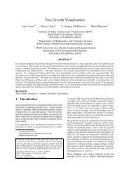
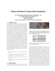
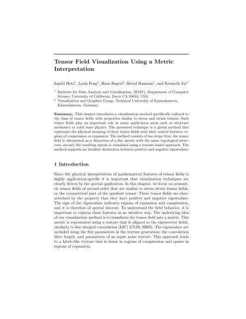
Tensor Field Visualization Using a MetricInterpretationIngrid Hotz 1 , Louis Feng 1 , Hans Hagen 2 , Bernd Hamann 1 , and Kenneth Joy 11 Institute for Data Analysis and Visualization, (IDAV), Department of ComputerScience, University of California, Davis CA 95616, USA2 Visualization and Graphics Group, Technical University of Kaiserslautern,Kaiserslautern, GermanySummary. This chapter introduces a visualization method specifically tailored tothe class of tensor fields with properties similar to stress and strain tensors. Suchtensor fields play an important role in many application areas such as structuremechanics or solid state physics. The presented technique is a global method thatrepresents the physical meaning of these tensor fields with their central features: regionsof compression or expansion. The method consists of two steps: first, the tensorfield is interpreted as a distortion of a flat metric with the same topological structure;second, the resulting metric is visualized using a texture-based approach. Themethod supports an intuitive distinction between positive and negative eigenvalues.1 IntroductionSince the physical interpretation of mathematical features of tensor fields ishighly application-specific it is important that visualization techniques areclosely driven by the special application. In this chapter, we focus on symmetrictensor fields of second order that are similar to stress strain tensor fields,or the symmetrical part of the gradient tensor. These tensor fields are characterizedby the property that they have positive and negative eigenvalues.The sign of the eigenvalues indicates regions of expansion and compression,and it is therefore of special interest. To understand the field behavior, it isimportant to express these features in an intuitive way. The underlying ideaof our visualization method is to transform the tensor field into a metric. Thismetric is represented using a texture that is aligned to the eigenvector fields,similarly to line integral convolution (LIC) [CL93, SH95]. The eigenvalues areincluded using the free parameters in the texture generation: the convolutionfilter length, and parameters of an input noise texture. This approach leadsto a fabric-like texture that is dense in regions of compression and sparse inregions of expansion.

2 Related WorkEven though several good visualization techniques exist for tensor fields, theyonly cover a few specific applications. Many of these methods are extensionsof vector field visualization methods, which focus on a technical generalizationwithout providing an intuitive physical interpretation of the resulting images.They often concentrate on the representation of eigendirections and neglectthe importance of the eigenvalues. Therefore, in many application areas traditionaltwo-dimensional plots are still used, which represent the interactionof two scalar variables.One way to represent a tensor field is based on using icons. They illustratethe characteristics of a field at some selected points (see, for example,[Hab90, KGM95, LW93]). Even though these icons represent the tensor valueat one point well they fail to provide a global view of the tensor field. A moreadvanced but still discrete approach uses hyperstreamlines. This approach isstrongly related to streamline methods used for vector fields. They were introducedby Delmarcelle and Hesselink [DH92] and have been utilized in ageomechanical context by Jeremic et al. [JSchF02]. Given a point in the field,one eigenvector field is used to generate a vector field streamline. The othertwo eigendirections and eigenvalues are represented by the cross section alongthe streamline. This method extracts more information than icons, but it stillleaves the problem of choosing appropriate seed points to the user. Thus, bothmethods have limited usage in exploration complete data sets and are limitedto low-resolution due to cluttering.To generate a more global view, a widely accepted solution for vectorfields is the reduction of the field to its topological structure. These methodsgenerate topologically similar regions that lead to a natural separation ofa field domain. The concept of topological segmentation was also appliedto two-dimensional tensor fields [HD95]. The topological skeleton consists ofdegenerated points and connecting separatrices. Degenerated points are wherethe tensor has multiple eigenvalues and the eigenvectors are not uniquelydefined. Although the tensor field can be reconstructed on the basis of itstopological structure, physical interpretation is difficult.Following an approach of Pang et al. [BP98, ZP02] a tensor field is consideredas a force field that deforms an object placed inside it. The localdeformation of probes, such as planes and spheres, illustrate the tensor field.This method only displays a part of the information because it reduces thetensor field to a vector field. To avoid visual clutter only a small numberof probes can be included in one picture Zheng et al. [ZPa03] extended thismethod by applying it to light rays that are bended by the local tensor value.Another class of visualization methods provides a continuous representation,based on textures. The first one to use a texture to visualize a tensorfield in a medical context were Ou and Hsu [OH01]. An approach based on theadaptation of LIC to tensor fields by Zheng et al. [ZP03]. Here, a white-noisetexture is blurred according to the tensor field. In contrast to LIC images,

the convolution filter is a two-dimensional or three- dimensional volume determinedby the local 2D or 3D tensor field respectively. This visualizationis especially good for showing the anisotropy of a tensor field. However, oneproblem of this method is the integration of the sign of the eigenvalues. Pointswith the same eigenvalues but with opposite sign are illustrated as isotropic.There exist some other techniques designed especially for the visualizationof diffusion tensors that only have positive eigenvalues. But they are notappropriate for stress, strain or gradient tensor fields.3 Metric DefinitionTo motivate our approach we discuss an example for the kind of tensor fieldswe are interested in. These are stress tensor fields and gradient tensor fieldswhose behavior is very similar, as a stress tensor is often computed as gradientof a virtual displacement field. It can be observe that for gradient fieldsor stress and strain tensors, positive eigenvalues lead to a separation of particlesor expansion of a probe. Eigenvalues equal to zero imply no change indistances, and negative eigenvalues indicate a convergence of the particles orcompression of the probe.For the symmetric part of a gradient tensor S of a vector field v =(v 1 , v 2 , v 3 ) with s ij = 1 2 (v i,j + v j,i ) this behavior is expressed by equation(1). Here, v i,j denotes the partial derivative of the ith component of v withrespect to coordinate x j .ddt (ds2 ) =3∑s ik dx i dx k =i,k=13∑λ j du 2 j. (1)Here, ds = (dx 1 ,dx 2 ,dx 3 ) and ds 2 is the quadratic distance of two neighboringpoints, λ j , j = 1, 2, 3 are the eigenvalues of S, and du j are the componentsof dx corresponding to the eigenvector basis {w j , j = 1, 2, 3}. If we focus onjust one eigendirection w i , the change of ds 2 is defined by the correspondingeigenvalue λ i :λ i > 0 → d dt ds2 > 0, λ i = 0 → d dt ds2 = 0, λ i < 0 → d dt ds2 < 0. (2)A similar behavior can be observed for the deformation of a probe in a stressfield (see Figure 1).Considering a time-independent vector field, a formal integration of Equation(1) results in the following expression for ds 2 :ds 2 (t) = ds 2 (0) + ∑ ikj=1(s ik · t) dx i dx k . (3)Usingds 2 (0) = a · ∑ dx i dx iiwe obtain:

ds 2 (t) = ∑ ik(aδ ik + s ik · t} {{ }=: g ik) dx i dx k , (4)where δ ik is the Kronecker-delta. The tensor g with components g ik =aδ ik + s ik · t can be interpreted as a time-dependent metric of the underlyingparameter space D. The constant a plays the role of a unit length, andt is a time variable that can be used as a scaling factor. This metric definitionis the basis of our tensor field visualization method.λ i > 0λ i = 0w iλ < 0 iFig. 1. Deformation of a unit probe under influence of a stress tensor in direction ofeigenvector w i. Eigenvalues larger than zero correspond to a tensile, and eigenvaluessmaller than zero to a compressive force in the direction of the eigenvector.3.1 The TransformationBased on the observations made in Section (3), we define a transformationof the tensor field into a metric. We do not exactly follow the motivatingEquation (4) but use a more flexible approach.Let T be a tensor field defined on a domain D. The tensor at a pointP ∈ D is given by T(P ). For each point P , the tensor T(P ) is mapped to ametric tensor g(P ) describing the metric in P . In the most general form, theassignment is achieved by the following three steps:1. Diagonalization of the tensor field:Switching from the original coordinate basis to the eigenvector basis {w 1 ,w 2 , w 3 }, we obtain a diagonal tensor T ′ having the eigenvalues of T on itsdiagonal:T ↦→ T ′ = U · T · U T = diag (λ 1 , λ 2 , λ 3 ) , (5)where U is the diagonalization matrix.2. Transformation and scaling of the eigenvalue, to define the metric g ′ accordingto the eigenvector basis:T ′ ↦→ g ′ = diag (F (λ 1 ), F (λ 2 ), F (λ 3 )) , (6)where F : [−λ max , λ max ] → IR + is a positive monotone function, withλ max = max{|λ i (P )|; P ∈ D, i = 1, 2, 3}.

3. Definition of the metric g in the original coordinate system by inverting thediagonalization defined in Equation (5):g = U T · g ′ · U. (7)If the mapping F is linear, the three steps can be combined into one step,and F can be applied to the tensor components, independently of the chosenbasis. The resulting metric g has the following properties:• It is positive definite and symmetric.• Its eigenvector field corresponds to the original eigenvector field of T.Thus, the tensor field topology in the sense of Delmarcelle et al. [HD95] ispreserved.• Its eigenvalues are given by F (λ j ). Positive eigenvalues are mapped tovalues greater than a, negative eigenvalues to values smaller than a butlarger then zero.The zero tensor is mapped to a multiple of the unit matrix.• Since the transformation is invertible, we get a one-to-one correspondenceof the metric and the tensor field is given.3.2 Examples for Transformation Functions F :In this paragraph we suggest some explicit definitions for the function F .Except from the first example all these functions are nonlinear and thereforecannot be directly applied to the tensor components. The functions we discusscan be classified in two groups:1. Anti-symmetric Treatment of the EigenvaluesTo underline the motivation defined by (4), we can define the transformationfunction as:F (λ) = a + σf(λ). (8)Here, a = F (0) defines the unit length, and σ ≠ 0 is an appropriate scalingfactor that guarantees that the resulting metric is positive definite. The functionf : IR → IR is a monotone function with f(0) = 0. If we want to treatpositive and negative Eigenvalues symmetrically it is f(−λ) = −f(λ). Fromthe large class of functions satisfying this condition we have considered threeexamples:a. Identity: f = id , f(λ) = λSince f is linear, the metric g is defined by g ij = F (t ij ) = a + σ · t ij . Thisequation corresponds exactly to our motivating Equation (4), where σ playsthe role of the time variable t. With σ < a/λ max we can guarantee that themetric is positive definite.b. Anti-symmetric logarithmic function:To emphasize regions where the eigenvalues change sign one can choose afunction f with a larger slope in the neighborhood of zero.

54c=2c=1010.8c=2c=52.5M320.60.42100.201.5−1−2−3−4−5−10 −5 0 5 10−0.2−0.4−0.6−0.8−1−4 −2 0 2 410.501−1/M−4 −2 0 2 4(a) (b) (c)Fig. 2. Figures (a) and (b) are examples for an anti-symmetric transformationfunction f. (a) Logarithmic function; (b) arc-tangent for two different slopes forλ = 0. Figure (c) is an example of a non-symmetric transformation function F fortwo different slopes at the origin.f(λ; c) ={log(c · λ + 1) for λ ≥ 0− log(1 − c · λ) for λ < 0 . (9)If we require σ < a/ log(c · λ max + 1) the resulting metric is positive definite.c. Asymptotic function:A function where the limitation of the scaling factor σ is independent of λ maxisf(λ; c) = arctan(c · λ), (10)with σ < 2a/π. For both functions, the constant c controls the “sharpness”at the zero crossing. For higher values of c the function becomes steeper, seeFigure 2.2. Non-symmetric function:As the visual perception of texture attributes is nonlinear, an anti-symmetricapproach is not always the best choice. An alternative that takes care of thisaspect is defined by the class of functions F [−λ max , λ max ] → [ a M, a·M], whereF (−λ) =a2F (λ) . (11)The constant a defines again the unit, aṀ the maximum, and a Mthe minimumvalue for F satisfying M > 1. Functions with this property can be obtainedby using anti-symmetric functions f as exponent:F (λ) = a · exp(σ · f(λ)) where f(−λ) = −f(λ). (12)An example for such a function with a = 1 is F (λ; c, σ) = exp(σ arctan(c · λ)).The constant c determines the slope of the function in the origin, see Figure2. The second class of functions produces much better results because thedifferences in the density of the resulting structure is more obvious. The specialchoice of the function f does not have a significant influence on the result.Another advantage of this class of functions F is that the resulting metric is

always positive definite and therefore, the scaling factor σ is not limited. Byan animation of this parameters we can enhance the impression of stretchingand compression.3.3 VisualizationWe now have transformed the problem of visualizing a tensor field to theproblem of visualizing an abstract metric. One way to solve this problem is anisometric embedding of the metric [Hot02]. The disadvantage of this approachis that it is restricted to two dimensions, and its existence is only guaranteedlocally. In general, several patches are needed to cover a field’s entire domain.Since we want to produce a global representation of a field we decided to followa different approach: Our basic idea is to use a texture that resembles a pieceof fabric to express the characteristic properties of the metric. The texture isstretched or compressed and bended according to the metric. Large values ofthe metric, which indicate large distances, are illustrated by a texture withlow density or a stretched piece of fabric. We use a dense texture for smallvalues of the metric. One can also think of a texture as probe inserted intothe tensor field.We generate the texture using LIC, a very popular method for vectorfield visualization. LIC blurs a noise image along the vector field or integralcurves. Blurring results in a high correlation of the pixel along field lines,whereas almost no correlation appears in direction perpendicular to the fieldlines. The resulting image leads to a very effective depiction of flow directioneverywhere, even in a dense vector field. LIC was introduced in 1993 by Cabraland Leedom [CL93]. Since the method was introduced, several extensions andimprovements were made to make it faster [SH95] and more flexible.We compute one LIC image for every eigenvector field to illustrate theeigendirections of the tensor field. For the integration of the integral curveswe use a Runge-Kutta method of fourth order, the LIC image is computedusing Fast-LIC as proposed in [SH95]. In each LIC image the eigenvalues ofevery eigenvector field are used to define the free parameters of the underlayingnoise image and the convolution. Finally, we overlay all resulting LIC imagesto obtain the fabric-like texture.Input Noise ImageWe use the free parameters of this input image to encode properties of themetric. Three basic parameters are changed according to the eigenvalues. Theyare: density, spot size, and color intensity of the spots. Considering theseparameters, the standard white-noise image is the noise image with maximumdensity, minimal spot size, and constant color intensity. It allows one to obtaina very good overall impression of the field; its resolution is only limited by pixelsize. Unfortunately, it is not flexible enough to integrate the eigenvalues whichrepresent fundamental field properties besides the directions. For this reason,

we use sparse noise input images, with lower density and larger spot size evenif we obtain a lower resolution. Some examples for different input images withchanging density and spot size are shown in Figure 3. The connection of theseparameters to the eigenvalues is explained in the following paragraphs:Density For each direction field w i , we define a specific density d i dependingon the orthogonal eigenvalues. A compression orthogonal to fibersleads to increasing density, and an expansion to decreasing density. For twodimensionaltextures this approach leads to the following definition of a onedimensionaldensity d i [spots/cm]:d i (λ) = d 0 ·1F (λ j ) , with j = {2 if i = 11 if i = 2|; ,(13)where F is defined by Equation (6), and d 0 defines the “unit-density,” d(0) =d 0 /F (0). In three dimensions, we have two orthogonal eigenvalues and thusobtain a direction-dependent density d i,j for each direction w j :d i,j (λ) = d 0 ·1F (λ j ) . (14)(a) (b) (c)Fig. 3. Example for different input images. (a) White noise image with maximumresolution; (b) spot noise image with changing density; (c) spot noise image withchanging spot size.Spot Size Increasing the radius of the underlying noise image leads tothicker; decreasing the radius leads to thinner fibers. This value is controlledby the orthogonal eigenvalues. In three dimensions, we define ellipsoids withthree different diameters according to the three eigenvalues:r i,j = r 0d i,j. (15)Convolution Length The defined noise image only uses the eigenvaluesorthogonal to the actual eigendirection field. A stretching or compressing in

the direction of the integral lines changes the length of the fibers. Fiber lengthis directly correlated to the length of the convolution filter l i , i.e.,l i = l 0 · F (λ i ). (16)(a) (b) (c) (d) (e)Fig. 4. Effect of changing image parameters for one eigenvector field of differentsimple synthetic tensor fields. In (a)-(c), only the input image is changed correspondingto the eigenvalues of the orthogonal eigenvector field; (a) change of density; (b)change of spot size; (c) change of density and spot size. Images (d) illustrates theeffect of changing the convolution length, where the parameters of the input noiseimage are constant. Image (e) shows a combination of the three parameters (density,spot size, and convolution length).(a) (b) (c)Fig. 5. Combination of two eigenvector fields, each representing both eigenvalues.In (a) and (b), only density and spot size are changed; (c) shows a combination ofthe three parameters.Color and Color Intensity In addition to these three “structure” parameters,color intensity can be used to enhance the impression of compressionand stretching. We use red for compression and green for tension. We applya continuous color mapping from red for the smallest negative eigenvalues,white for zero eigenvalues, and green for positive eigenvalues. The definitionof the different parameters for three dimensions is summarized in Table 1.

4 Results and ConclusionsWe have evaluated our method using synthetic and real data sets. Simpletensor fields, where the eigenvector fields are aligned to the coordinate axes,have allowed us to validate the effect of changing texture parameters. We haveobtained similar results for datasets where the eigenvector fields are rotatedby 90 degrees. Results where only one eigenvector field is used are shown inFigure 4. Images for the same datasets showing both eigendirections are shownin Figure 5. We have used different input textures and parameter mappings.The next examples are results for simulated finite element data sets ofthe stress field resulting from applying different load combinations to a solidblock. These datasets are well-studied and therefore appropriate to evaluateour method. For the simulation, a ten-by-ten-by-ten gird had been used. Thetensor field resulting from the simulation is continuous inside each cell, butnot on cell boundaries. This fact can be observed in our images. Figure 6and Figure 7 (see color plates) show different slices of the three-dimensionaldataset from a single point load. Figure 8 (see color plates) represents a blockwhere two forces with opposite sign were applied. These images provide agood visual segmentation of regions of compression and expansion.(a) (b) (c)Fig. 6. Images showing a yz-plane slice of single top-load data set, where a force isapplied in z-direction. (a) and (b) illustrate the two eigenvector fields separately; in(c) they are overlaid. In all images, spot size and density are changed according toeigenvalues.The interpretation of a tensor field as a distortion of a flat metric canbe used to produce a visualization based on the real physical effect of thetensor field. The distortion of the texture according to the metric supports aflexible representation of two-dimensional slices of a tensor field, which is easyto understand. An extension to three dimensions is possible but there is stillthe problem of cluttering which must be solved.

eigenvector fieldfree parameters i = 1 i = 2 i = 3density value d i,j1λ 21λ 11λ 1d i,k1λ 21λ 11λ 11 1 1color intensity I i λ 1 λ 2 λ 3convolution length l i λ 1 λ 2 λ 3spot diameter r i,j λ 2 λ 3 λ 1r i,k λ 3 λ 1 λ 2Table 1. Assignment of eigenvalues to free parameters for a three-dimensional texture.References[BP98] Ed Boring and Alex Pang. Interactive Deformations from Tensor Fields.Proceedings of the Visualization ’98 Conference, 1998, pages 297-304.[CL93] Brian Cabral and Leith Leedom. Imaging Vector Fields Using Line IntegralConvolution. In SIGGRAPH ’93 Conference Proceedings, 1993, pages263-272.[DH92] Thierry Delmarcelle and Lambertus Hesselink. Visualization of secondorder tensor fields and matrix data. Proceedings of the Visualization ’92Conference, 1992, pages 316-323.[Hab90] Robert B. Haber. Visualization Techniques for Engineering Mechanics. InComputing Systems in Engineering, 1990, pages 37-50.[HD95] Lambertus Hesselink, Thierry Delmarcelle and James L. Helman . Topologyof Second-Order Tensor Fields. In Computers in Physics, 1995, pages304-311.[Hot02] Ingrid Hotz. Isometric Embedding by Surface Reconstruction from Distances.Proceedings of the IEEE Visualization ’02 Conference, 2002, pages251-258.[HFHHJ04] Ingrid Hotz, Louis Feng, Hans Hagen, Bernd Hamann, Boris Jeremic,and Kenneth Joy. Physically Based Methods for Tensor Field Visualization.Proceedings of the IEEE Visualization ’04 Conference, 2004, pages123-130.[JSchF02] Boris Jeremic, Gerik Scheuermann and Jan Frey et al. Tensor Visualizationin Computational Geomechanics. In International Journal for Numericaland Analytical Methods in Geomechanics, 2002, pages 925-944.[KGM95] Ron D. Kriz, Edward H. Glaessgen and J.D. MacRae. Visualization Blackboard:Visualizing gradients in composite design and fabrication. IEEEComputer Graphics and Applications, vol 15, 1995, pages 10-13[LW93] W. C. de Leeuw and J. J. van Wijk. A Probe for Local Flow Field Visualization.Proceedings of the Visualization ’93 Conference, 1993, pages39-45.[OH01] J. Ou and E. Hsu. Generalized Line Integral Convolution Rendering ofDiffusion Tensor Fields. Proceedings of the 9th Scientific Meeting and Exhibitionof the International Society for Magnetic Resonance in Medicine(ISMRM), page 790, 2001.

[SH95][ZP02][ZPa03][ZP03]Detlev Stalling and Hans-Christian Hege. Fast and Resolution IndependentLine Integral Convolution. In SIGGRAPH ’95 Conference Proceedings,1995, pages 149-256.Xiaoqiang Zheng and Alex Pang. Volume Deformation For Tensor Visualization.Proceedings of the Visualization ’02 Conference, 2002, pages379-386.Xiaoqiang Zheng and Alex Pang. Interaction of Light and Tensor Field.Proceedings of VISSYM ’03, 2003, pages 157-166.Xiaoqiang Zheng and Alex Pang. HyperLIC, Proceedings of the IEEEVisualization ’03 Conference, 2003, pages 249–256.

(a)(b)Fig. 7. This figure shows a single-top-load. Spot size and density of the input imagesare adapted to the corresponding eigenvectors. Red shows regions of compression,green expansion according the respective eigenvector field: the images are planarslices along the (a) yz-plane and (b) xy-plane slice orthogonal to the force.(a)(b)Fig. 8. The images represents a yz-plane (a) and xz-plane (b) slice of a two-forcedataset. (a): In the lower-left corner we see a region of compression, a result mainlydue to the pushing force on the left; in the upper-right corner expansion dominatesas a result of the right pulling force. (b): The left circle corresponds to the pushingand the right to the pulling force. The fluctuation of the color is a result of the lowresolution of the simulation.