proper feedback compensators for a strictly proper plant

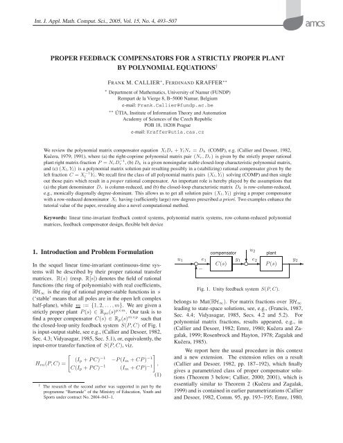
Int. J. Appl. Math. Comput. Sci., 2005, Vol. 15, No. 4, 493–507PROPER FEEDBACK COMPENSATORS FOR A STRICTLY PROPER PLANTBY POLYNOMIAL EQUATIONS †FRANK M. CALLIER ∗ ,FERDINAND KRAFFER ∗∗∗ Department of Mathematics, University of Namur (FUNDP)Rempart de la Vierge 8, B–5000 Namur, Belgiume-mail: Frank.Callier@fundp.ac.be∗∗ ÚTIA, Institute of Information Theory and AutomationAcademy of Sciences of the Czech RepublicPOB 18, 18208 Praguee-mail: Kraffer@utia.cas.czWe review the polynomial matrix compensator equation X l D r + Y l N r = D k (COMP), e.g. (Callier and Desoer, 1982,Kučera, 1979; 1991), where (a) the right-coprime polynomial matrix pair (N r,D r) is given by the strictly proper rationalplant right matrix-fraction P = N rDr−1 ,(b)D k is a given nonsingular stable closed-loop characteristic polynomial matrix,and (c) (X l ,Y l ) is a polynomial matrix solution pair resulting possibly in a (stabilizing) rational compensator given by theleft fraction C = X −1lY l . We recall first the class of all polynomial matrix pairs (X l ,Y l ) solving (COMP) and then singleout those pairs which result in a proper rational compensator. An important role is hereby played by the assumptions that(a) the plant denominator D r is column-reduced, and (b) the closed-loop characteristic matrix D k is row-column-reduced,e.g., monically diagonally degree-dominant. This allows us to get all solution pairs (X l ,Y l ) giving a proper compensatorwith a row-reduced denominator X l having (sufficiently large) row degrees prescribed apriori. Two examples enhance thetutorial value of the paper, revealing also a novel computational method.Keywords: linear time-invariant feedback control systems, polynomial matrix systems, row-column-reduced polynomialmatrices, feedback compensator design, flexible belt device1. Introduction and Problem FormulationIn the sequel linear time-invariant continuous-time systemswill be described by their proper rational transfermatrices. R(s) (resp. R[s]) denotes the field of rationalfunctions (the ring of polynomials) with real coefficients,RH ∞ is the ring of rational proper-stable functions in s(‘stable’ means that all poles are in the open left complexhalf-plane), while m := {1, 2,...,m}. We are given astrictly proper plant P (s) ∈ R po (s) p×m . Our task is tofind a proper compensator C(s) ∈ R p (s) m×p such thatthe closed-loop unity feedback system S(P, C) of Fig. 1is input-output stable, see e.g., (Callier and Desoer, 1982,Sec. 4.3; Vidyasagar, 1985, Sec. 5.1), or, equivalently, theinput-error transfer function of S(P, C), viz.[](I p + PC) −1 −P (I m + CP) −1H eu (P, C) =C(I p + PC) −1 (I m + CP) −1 ,(1)† The research of the second author was supported in part by theprogramme “Barrande” of the Ministry of Education, Youth andSports under contract No. 2004–043–1.compensatorplantu 1 e 1 y 1 e 2 y✲ ❡ ✲ ❡ 2C(s) ✲ ❄ ✲ P (s) ✲✻−u 2Fig. 1. Unity feedback system S(P, C).belongs to Mat(RH ∞ ). For matrix fractions over RH ∞leading to state-space solutions, see, e.g., (Francis, 1987,Sec. 4.4; Vidyasagar, 1985, Secs. 4.2 and 5.2). Forpolynomial matrix fractions, results appeared, e.g., in(Callier and Desoer, 1982; Emre, 1980; Kučera and Zagalak,1999; Rosenbrock and Hayton, 1978; Zagalak andKučera, 1985).We report here the usual procedure in this contextand a new extension. The extension relies on a result(Callier and Desoer, 1982, pp. 187–192), which finallygives a parametrized class of proper compensator solutions(Theorem 3 below; Callier, 2000; 2001), which isessentially similar to Theorem 2 (Kučera and Zagalak,1999) and is contained in earlier parametrizations (Callierand Desoer, 1982, Comm. 95, pp. 193–195; Emre, 1980,

Proper feedback compensators for a strictly proper plant by polynomial equations495a right polynomial matrix fraction of P (s) ∈ R(s) p×m ,then so is (N r R, D r R), where R is any unimodular matrix.Moreover, right-coprimeness is invariant under thistransformation. This allows simultaneous elementary columnoperations on the numerator and denominator suchthat the latter gets column-reduced. A similar commentis valid for left fractions, left multiplication by a unimodularmatrix, and elementary row operations leading to arow-reduced left denominator.Definition 1. An m × m polynomial matrix D is saidto be column-reduced if it has m column degrees k j :=δ cj [D] such that the limitD h := lim D(s)diag[ s ] −kj m(10)s→∞ j=1exists and is nonsingular.Comment 1. An equivalent requirement is thatD − (s) := D(s)diag [ ] ms −kj is a biproper rationalmatrix. One gets D h = D − (∞) and D h is calledj=1the highest column degree coefficient matrix of D(s).In (Wolovich, 1974, p. 27), “column-reduced” is termed“column-proper.”Definition 2. An m × m polynomial matrix D is saidto be row-reduced if it has m row degrees r i := δ ri [D]such that the limitD h := lim diag [ s −ri] mD(s) (11)s→∞ i=1exists and is nonsingular.Comment 2. An equivalent requirement is thatD − (s) := diag[s −ri ] m i=1D(s) is a biproper rationalmatrix. One gets D h = D − (∞) and D h is calledthe highest row degree coefficient matrix of D(s). In(Wolovich, 1974), “row-reduced” is termed “row-proper.”Remark 2. Column degrees and column-reducedness areappropriate tools for revealing that a right polynomial matrixfraction is proper. Indeed, it is well known, see e.g.,(Callier and Desoer, 1982, p. 70; Kailath, 1980, p. 385),that with (N(s),D(s)) ∈ Mat(R[s]) and D(s) columnreduced,G(s) := N(s)D −1 (s) ∈ R(s) p×m is proper(resp. strictly proper) iff for all j ∈ m, δ cj [N] ≤ δ cj [D](resp. δ cj [N] < δ cj [D]). A similar comment can bemade for left fractions, row degrees and row-reducedness.What is paramount here is the fact that the degree of anentry of a polynomial matrix is limited column-wise byits column-maximum or row-wise by its row-maximum,viz. by the corresponding column degree or row degree.This way of control is less appropriate when the matrixD k in (COMP) is a sum having a dominant term, whichis a product of a row-reduced matrix X l and a columnreducedmatrix D r .Theorem 1 below shows that the following is appropriate.Definition 3. (Callier and Desoer, 1982, p. 116) Anm × m polynomial matrix D is said to be row-columnreducedif there exist m nonnegative integers r i , calledrow powers, and m nonnegative integers k j , called columnpowers, such that the limitD h := lims→∞ diag [ s −ri] mi=1 D(s)diag[ s −kj ] mj=1(12)exists and is nonsingular.Comment 3. An equivalent requirement is thatD − (s) := diag[s −ri ] m i=1 D(s)diag[ ] ms −kj is aj=1biproper rational matrix. One gets D h = D − (∞) andD h is called the highest degree coefficient matrix ofD(s). Another interpretation of the definition is that forall (i, j) ∈ m × m, δ ij [D] ≤ r i + k j with nonsingulardegree-contact (nonsingular D h ). What is important hereis the fact that the degrees of the entries are bilaterallycontrolled, i.e. with row and column powers; these powersare generically not unique, as will be observed below.In the sequel c.r., r.r., and r.c.r. are abbreviations forcolumn-reduced, row-reduced, and row-column-reduced.There are many r.c.r. nonsingular polynomial matrices.Rosenbrock has already considered the idea of the definitionfor D h = I. Note here, see, e.g., (Callier and Desoer,1982, Sec. 2.4; Kailath, 1980, Sec. 6.3) that any nonsingularpolynomial matrix D can be reduced to its Smithform S by elementary row and column operations, i.e.,D = LSR with L and R unimodular matrices.Fact 1. (Rosenbrock and Hayton, 1978, Lem. 1) DenoteSmith forms as S = diag[φ i ] m i=1 with δ[φ 1] ≥ δ[φ 2 ] ≥··· ≥ δ[φ m ]. Consider m nonnegative integers r i suchthat r 1 ≥ r 2 ≥ ··· ≥ r m , and m nonnegative integersk j such that k 1 ≥ k 2 ≥···≥k m .Then, there exists a nonsingular r.c.r. polynomial matrixD having the Smith form S and having row powersr i , column powers k j , and D h = I, if and only ifk∑δ[φ i ] ≥i=1k∑(r i + k i ), for k ∈ m, (13)i=1with equality for k = m.It follows from this fact that many nonsingular polynomialmatrices can be made r.c.r. by elementary operations.The star case of row-column-reducedness is, however,probably reflected by the following case containedin the proof of Fact 1.

496Definition 4. An m × m polynomial matrix D is said tobe monically diagonally degree dominant with diagonaldegrees γ i (i ∈ m) if every diagonal entry of D is monicand for (i, j) ∈ m × m with i ≠ j and γ i := δ ii [D],δ ij [D] < min (γ i ,γ j ). (14)Comment 4. Here, without loss of generality, by symmetricpermutations, γ 1 ≥ γ 2 ≥···≥γ m , giving, e.g., adegree matrix⎡⎢⎣5 3 22 4 21 2 3⎤⎥⎦ .Observe that this is easily obtained: get a “diagonal degreeridge” with “top degrees on the diagonal.”Fact 2. Let D be an m × m nonsingular polynomialmatrix. Consider m nonnegative integers γ i such thatγ 1 ≥ γ 2 ≥ ··· ≥ γ m . Then the following assertions areequivalent:(a) D is c.r. with column degrees γ i and D h = I,simultaneously D is r.r. with row degrees γ i andD h = I.(b) D is monically diagonally degree dominant with diagonaldegrees γ i , i ∈ m.(c) D is r.c.r. with row powers r i , column powers k jand D h = I, for all pairs of m-tuples of nonnegativeintegers r i and k j such that r 1 ≥ r 2 ≥ ··· ≥r m , and k 1 ≥ k 2 ≥···≥k m , and γ i = r i + k i forall i ∈ m.Proof. We show the chain of implications (a) ⇒ (b) ⇒(c) ⇒ (a). The first implication is straightforward. Forthe second one, observe that here: (i) for all i = j, d iiis monic with δ ii [D] =γ i = r i + k i , (ii) for all i>j,δ ij [D]

Proper feedback compensators for a strictly proper plant by polynomial equations497S(P, C) of Fig. 1 has a polynomial matrix system description,e.g., (Callier and Desoer, 1982),⎧ )⎪⎨S(P, C) : [( dD k ξ(t)dt[ ( ) d= Y ldty 1 (t)y 2 (t)X l( ddt⎡ (] dD r= ⎢dt⎣( dN r[ dt0 −I m+0 0) ] [ ]u 1 (t),u 2 (t)) ⎤) ⎥⎦ ξ(t)][ ]u 1 (t)⎪⎩.u 2 (t)(16)The system S(P, C) is well formed (Callier and Desoer,1982, Sec. 3.3) and has its zero-input dynamicsfixed aprioriby the data D r , N r ,andD k ; its zerostatedynamics are ultimately fixed by a solution X l ,Y l of (COMP). Moreover, when all degree control parametersare positive, it is possible to get (A, B, C, D),a Fuhrmann-inspired state-space realization (Fuhrmann,1976, Sec. VI), where the plant and the characteristic matrixD k fix A and C, and the compensator fixes Band D. The order n of the system S(P, C) equals thenumber of independent initial conditions ξ j (0 − ) (k) , j ∈m, k = {0, 1,...} needed to determine a solution ξ(t)of the homogeneous equation D k ( d dt)ξ(t) =0obtainedin (16) by putting u 1 =0, u 2 =0, t ≥ 0.In view of Theorem 1 and earlier comments, the importantexistence question is: Assuming that Condition (a)holds, when does (b) hold? The answer is: by choosingthe row powers r i of the closed-loop characteristic denominatorD k sufficiently large. Indeed, one has the followingresult, whose proof is given for the reader’s convenience.Theorem 2 (Particular proper compensator). (Callierand Desoer, 1982, p. 190) Let P (s) ∈ R po (s) p×m havecoprime right and left polynomial matrix fractions readingP (s) =N r (s)D r (s) −1 = D l (s) −1 N l (s), (17)with D r c.r. with column degrees k j (j ∈ m) and D lr.r. with row degrees μ i (i ∈ p). Let μ := max i∈p μ i ,i.e., μ is the greatest observability index of the plant, cf.(Kailath, 1980, p. 431). Let(a) D k ∈ R[s] m×m be r.c.r. with row powers r i andcolumn powers k j , and(b) r i ≥ μ − 1 for all i ∈ m.Then for the given data D k , N r and D r , (COMP) has apolynomial matrix solution (X l ,Y l ) such that δ ri [Y l ] ≤r i for all i ∈ m. Hence (by Theorem 1) X l is r.r. withrow degrees r i and C(s) =X l (s) −1 Y l (s) ∈ R p (s) p×m .Proof. All polynomial matrix solutions of (COMP) aregiven by the pairs (X l ,Y l ) given by (8), where N k ∈Mat(R[s]) is a free parameter. In Y lp = −N k D l + Y l ,choose −N k and Y l to be the quotient and remainder ofthe division of Y lp on the right by D l .ThenY l D −1lisstrictly proper such that δ cj [Y l ] < δ cj [D l ] for all j ∈p. Hence for all i ∈ m δ ri [Y l ] ≤ max i∈m δ ri [Y l ] =max j∈p δ cj [Y l ] < max j∈p δ cj [D l ]=max i∈p δ ri [D l ]:=μ. Thus for all i ∈ m one gets δ ri [Y l ] ≤ μ − 1 ≤ r i .Comment 7. The idea of the proof of Theorem 2 is usedin the proof of (Rosenbrock and Hayton, 1978, Thm. 6).However, one does not need to resort to the division ofY lp on the right by D l to obtain an existence result; see,e.g., (Emre, 1980, Thm. 4.1; Kraffer and Zagalak, 2002,Lem. 4.2; Antoniou and Vardulakis, 2005) for anothermethod.The following result constitutes, together with Theorem2, a generalization of Theorem 2 in (Kučera and Zagalak,1999) (modulo dualization and the fact that rowcolumn-reducednessof D k is used instead of the morerestricted assumption that D k is simultaneously row- andcolumn-reduced, see Fact 2). It forms a parametrized classof solutions to (COMP) leading to a proper compensator.Its simple proof here is based on Theorem 1.Theorem 3 (Parametrization of proper compensators).Let the assumptions of Theorem 1 hold with P (s) havingcoprime right and left polynomial matrix fractionsas in (17), and let D k satisfy Condition (a) of Theorem1 with row powers r i (i ∈ m). Moreover, assumethat a particular solution (X lo ,Y lo ) of (COMP) existssuch that X lo is r.r. with row degrees r i (i ∈ m), andC o := X −1lo Y lo ∈ R p (s) m×p .Then all polynomial matrix solutions (X l ,Y l ) of(COMP) such that X l is r.r. with row degrees r i (i ∈ m),and C := X −1lY l ∈ R p (s) m×p are given byX l = X lo − N k N l , Y l = Y lo + N k D l , (18)where N k ∈ R[s] m×p has the property that for all i ∈ mand for all j ∈ p,δ ij [N k ] ≤ r i − μ j = r i − δ rj [D l ]. (19)Proof. Define Δ µ (s) := diag[s µi ] p i=1 and Δ r(s) :=diag [s ri ] m i=1. Note that by Theorem 1, Δ−1 r Y lo is proper.Observe also that condition (b) of Theorem 1 is equivalentto requiring that Δ −1r Y l be proper. Finally, as D l

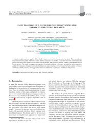
498F.M. Callier and F. Krafferθ 1,ω 1,M 1 θ 2,ω 2,M 2Fig. 2. Laboratory flexible belt coupled drive system.is r.r. with row-degrees μ i , one gets by Comm. 2 thatD l =Δ µ D l− ,where D l− is biproper. Hence upon substitutingthis in the second equation of (18) premultipliedby Δ −1r , one gets Δ −1r Y l =Δ −1r Y lo +Δ −1r N k Δ µ D l− ,where Δ −1r Y lo is proper and D l− is biproper. ThusΔ −1r Y l is proper iff Δ −1r N k Δ µ is proper. The result followsfrom this and Theorem 1.Comment 8. The parametrization in (18) is only relativelynew as it is contained in earlier affine parametrizationsgenerated by Emre (1980, Rem. 3.4) and Callierand Desoer (1982, Comm. 95, pp. 193–195), i.e., solvingalgebraic linear systems with fewer equations than unknowns:the solution contains free parameters which canbe adapted to those of Theorem 3. This is also the case for(Antoniou and Vardulakis, 2005, Thm. 8) and in a similarfashion for (Kraffer and Zagalak, 2002), which handlesessentially the case r i = μ − 1 for all i ∈ m.5. Control Laboratory Tracking DeviceExampleOur first example concerns a control laboratory device,viz. the flexible belt coupled drives system of Fig. 2. Thesystem has three actuators, two motors and a tensioner,equipped with pulleys, which are centered at the verticesof an isosceles triangle of varying height. A continuousflexible belt is moved by these pulleys. The lower twopulleys (driven pulleys) have fixed centers and are drivenby two identical voltage controlled electric DC servomotors,with common drive voltage u d = u 1 = u 2 . Theupper pulley (jockey pulley) has a center that can be verticallydisplaced by a tensioner bar, controlled by a voltagedriven electromagnet and containing a spring-dashpotsystem whose spring may be simplified to a linear spring.The actuators operate simultaneously to control the speedof the belt and its tension. The vertical displacement ofthe center of the jockey pulley and thus of the tensioner isa measure of the tension in the belt. It is assumed that thebelt speeds at the driven pulleys are the circumferentialspeeds of these pulleys due to the servomotors, and thatthe belt speed is the average of the belt speeds at the drivenpulleys. The outputs of interest are the belt speed and thevertical position of the tensioner. Assuming that the beltangle α is constant, a linear initial model (ProTyS, Inc.,2003; Hagadoorn and Readman, 2004) is given byẋ(t) =Ax(t)+Bu(t),y(t) =Cx(t),a minimal state-space realization specified by(20)⎡⎤0 0.0310 −0.0310 0 0−44286 −3.0786 0 34197 0A=44286 0 −3.0786 −34197 0,⎢⎣0 0 0 0 1.0000 ⎥⎦514.80 0 0 −1128.4 −66.667(21)

Proper feedback compensators for a strictly proper plant by polynomial equationsB =C =⎡⎢⎣0 02076.4 02076.4 00 00 −51.000⎤⎥⎦ , (22)[ 0 0.0008060 0.0008060 0 00 0 0 −66.000 0(23)In the sequel we shall use the notation of Fig. 2 asmuch as possible. The states contained in x are successively:horizontal belt length change due to the electricdrives x h = r(θ 1 − θ 2 ) [m], left motor angular velocityω 1 =dθ 1 /dt [rad/s], right motor angular velocityω 2 = dθ 2 /dt [rad/s], tensioner vertical position x k [m]and tensioner vertical speed v k [m/s]. The inputs in uare successively: common drive voltage u d and electromagnetvoltage u k . The outputs in y are: belt speedr(ω 1 + ω 2 )/2 and tensioner vertical position x k . Bothu and y are measured in computer units [–].The dynamic responses of the currents of the drivecircuits of the motors and electromagnet are much fasterthan those of the mechanical variables, whence the inductancesof the former circuits are neglected. This gives forthe motor torques M i = βu d − β e ω i (i =1, 2), whereβ is the drive voltage constant and β e is a constant due tothe back electromotive force (Messner and Tilbury, 1999).Moreover, for the vertical force applied by the electromagnetF m = β k u k ,whereβ k is the electromagnet voltageconstant. An important parameter is the oblique beltlength change, which, assuming that the belt position atthe jockey pulley is r(θ 1 + θ 2 )/2, gives for the left caser[(θ 1 +θ 2 )/2−θ 1 ]+(cosα)x k = −(1/2)x h +(cosα)x k ,and the same result for the right case. The most importantstate differential equations are the second, third and lastone (for the notation see above and Fig. 2). They concern:(i) the balances of the torques applied to the left and rightdriven pulleys, namely,J dω (11)= −(B + β e )ω 1 −dt2 k g1 + k g2 rx h+ k g1 r(cos α)x k + βu d ,J dω 2dt= −(B + β e )ω 2 +( 12 k g1 + k g2)rx h− k g1 r(cos α)x k + βu d ,and (ii) the balance of the vertical forces applied to thetensioner, namely,dv km k = −B k v k − (k k +2k g1 cos 2 α)x kdt+ k g1 (cos α)x h − β k u k ,where k g1 and k g2 are belt stiffness constants.].499Our task is to design a proper compensator such thatthe closed-loop unity feedback system can track referencesignals. These concern here the outputs, viz., belt speedand tensioner vertical position of the model given aboverepresented by a strictly proper plant P(s) ∈ R po (s) 2×2 ,i.e.,P(s) =C(sI −A) −1 B. (24)Design specifications include the capability of respondingto setpoint values that may change from timeto time (step changes). In absolute value physical capabilitiesand limitations on actuators require the drive inputand tensioner voltages to stay below 0.8 [–] and 0.4 [–],respectively, for the belt speed and tensioner position below0.25 [–] and 0.35 [–], respectively.A conventional solution to the task relies on a statespace approach, viz., linear quadratic optimal control(Athans and Falb, 1966), involving a state-variable feedbackcontrol law and an asymptotic estimator for providingan estimate of the state-variables not present in theoutput, and where, moreover, preliminary use of integralcontrol is needed because our plant has no integral actionof its own.Our solution to the task relies on polynomial equationsand is inspired by the conventional approach, butachieved by the design of a compensator, which is directlyobtained; the estimator and integral control occurimplicitly and are not done separately. As in state spacedesign, one uses constant, positive weights for tuning. Animportant advantage of the present technique is that thearbitrariness is reduced to fewer degrees of freedom thanthose required to select the weights in a higher-order statespace system.Near physical symmetry with respect to the verticalaxis through the tensioner bar in Fig. 2 revealsthat a simplified model can be obtained from the initialmodel (20)–(24). First, we replace the state vector(x h ,ω 1 ,ω 2 ,x k ,v k ) T by (x h , (ω 1 + ω 2 )/2, (ω 1 −ω 2 )/2,x k ,v k ) T . During tests it is then observed that thestates x h = r(θ 1 − θ 2 ) and (ω 1 − ω 2 )/2 remain smallwithin the range of design specifications, whence theymay be set to zero and removed. Thus we get a final simplifiedmodel in terms of a minimal state-space realization(A, B, C) specified by[ ]A BC 0⎡=⎢⎣−3.0786 0 0 2076.4 00 0 1.000 0 00 −1128.4 −66.667 0 −51.0000.0008060 0 0 0 00 −66.000 0 0 0⎤.⎥⎦(25)

500The states are here successively: average driven pulleyangular velocity (ω 1 + ω 2 )/2 [rad/s], tensioner verticalposition x k [m], and tensioner vertical speed v k [m/s].The inputs are: common drive input voltage u d , and electromagnetvoltage u k , and the outputs are: average beltspeed r(ω 1 + ω 2 )/2 and tensioner vertical position x k .Both inputs and outputs are in computer units [–].The simplified model can be represented by the coprimeright polynomial matrix fractionP (s) =N r (s)D r (s) −1 , (26)where the polynomial matrices N r and D r are given by⎡⎤[ ]1.6736 0N r (s)0 3366.0= ⎢⎥D r (s) ⎣ s +3.0786 0 ⎦ .0 s 2 +66.667s + 1128.4(27)For future reference, record that the column degrees ofD r are (k 1 ,k 2 )=(1, 2), the right and left fractions ofP coincide (the transfer function is diagonal), and its observabilityindex equals two, the largest row degree in theleft denominator (Kailath, 1980).We choose now an appropriate matrix D k for theplant (26)–(27) to set up an appropriate compensatorequation (COMP).Guided by LQ-optimal control methods, we computefirst the polynomial matrixW (s)[]0.70711s+2.7459 0=0 2.2361s 2 ,+172.49s+4206.7(28)whose zeros are exclusively in the open left half-plane.The matrix W is obtained from spectral factorizationgiven by[ ][]W T (−s)W (s)= Nr T(−s) DT r (−s) N r (s)S,D r (s)(29)where S is a positive-definite matrix, a design parameterweighting the importance of inputs and outputs relative tothe partial states of N r D −1 . The weight S is selected asrS = diag(1, 1, 0.5, 5). (30)The spectral factor W is r.c.r. with row and column powersgiven by (r 1 ,r 2 ) = (0, 0) and (k 1 ,k 2 ) = (1, 2).Hence, as was to be expected, by Theorem 1 with D k =W only a constant compensator can be obtained from theequation(COMP),andwehavetofind a matrix D k thatF.M. Callier and F. Krafferis r.c.r. with identical column powers and strictly largerrow powers for obtaining a dynamical compensator that(i) contains a full rank integrator, capable of tracking inputreference signals, and (ii) provides for “good observerdynamics.”Our final choice is the polynomial matrixD k (s) =[]d k 11(s) 00 d k 22 (s) , (31)where d k 11(s) =s 2 +7.8832s +15.533 and d k 22(s) =s 4 +95.138s 3 +3325.8s 2 +38183s+105350. It is obtainedby scaling the diagonal elements to monic polynomials ofthe diagonal matrix QW ,where Q is a “good augmenteddynamics” scaling factor selected asQ(s) =[s +4 00 (s +4)(s + 14)and W is the spectral factor in (28).], (32)The matrix D k is trivially monically diagonallydominant with diagonal degrees (2, 4), and r.c.r. with rowand column powers (r 1 ,r 2 ) = (1, 2) and (k 1 ,k 2 ) =(1, 2).For the data (D r ,N r ,D k ) in (27) and (31), byTheorems 1 and 2, proper compensators (X l ,Y l ) withδ ri [X l ]=r i (i =1, 2) for (r 1 ,r 2 )=(1, 2) exist. Aparticular proper compensator is given byC(s) =[×s +4.8047 00 s 2 +28.471s + 299.30[0.44302 00 −4.1287s − 69.037] −1]. (33)This compensator, obtained by the method in (Kraffer andZagalak, 2002, Lem. 4.2), is not unique. Non-uniquenessis a generic property, not valid given our data should therow powers of D k equal the lower bound μ − 1=1given by Theorem 2. As one of the row powers D k ,givenabove, exceeds the lower bound, extra degrees of freedomare generated that are available to accommodate theopen-loop system consisting of the compensator C andthe plant P such that [I + PC] −1 (0) = 0, i.e., as a systemwhich is able to track steps under unity feedback.For the data (D r ,N r ,D k ) in (27) and (31), theaffine set of all proper compensators, with δ ri [X l ]=r i(i = 1, 2), may be centered on the compensator givenby (33). Since here (r 1 ,r 2 ) = (1, 2) and (μ 1 ,μ 2 ) =(1, 2), a parametrization of this set is given by Theorem 3

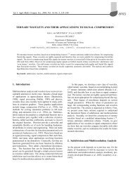
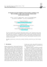
Proper feedback compensators for a strictly proper plant by polynomial equations501by[X l (s) =Y l (s) =]s +4.8047 00 s 2 +28.471s + 299.30− N k (s)[+N k (s)[]1.6736 0, (34)0 3366.0]0.44302 00 −4.1287s − 69.037[]s+3.0786 00 s 2 , (35)+66.667s+1128.4where the free parameter N k has the form[]n 1 0N k (s) =, (36)m 21 s + n 21 n 2all coefficients being free.In order to obtain a simple, i.e., diagonal compensator,we set m 21 = n 21 =0 and satisfy the tracking objectiveby finding a diagonal constant value of N k suchthat [I + PC] −1 (0) = 0, here X l (0) = 0. As a consequence,the value of N k is unique,[]2.8709 0N k =, (37)0 0.08892and specifies the compensator given by[]s 0X l (s) =0 s 2 , (38)+28.471sY l (s)[]2.8709s+9.2811 0=0 0.08892s 2 .+1.7993s+31.299(39)As was to be expected by the internal model principle, thecompensator contains a full rank integrator, and, exceptfor its pole at zero, is stable. Moreover, it is minimumphase. This is considered good for practical applications.Having designed our tracking compensator using thesimplified model in (26)–(27), we return to the initialmodel (20)–(24) to verify the corresponding closed-loopdesign performance.The results are shown in Fig. 3. Verification using theactual physical system is shown in Fig. 4. In both figuresthe upper three curves concern tensioner variables, and thelower three concern belt speed variables. The nonzero displacementof the tensioner at the start of the run in Fig. 4is due to (unmodeled) static friction. The results are satisfactory.The steps of the method to design a tracking compensatorwere as follows: (a) select a convenient representationof the plant-sensor-actuator, in the form of a coprimeright polynomial matrix fraction, (b) develop theright hand-side matrix for (COMP) that corresponds tosatisfactory dynamic response, based on a suitable balanceof weighted spectral factorization and additionallyselected poles, and (c) customize the solution of (COMP)such that the open-loop system satisfies the internal modelprinciple, that is, endow the system with the ability to generate,and hence also to track, a given class of signals.6. Example for Comparison with OtherMethodsFor educational purposes and for straightforward numericalevidence, we introduce a simple example, which isamenable to hand calculations. Consider the followingunstable plant with a strictly proper transfer matrix:P (s) =⎡⎢⎣s +1s(s − 2)1s(s − 1)01s − 1⎤⎥⎦ , (40)with coprime right and left polynomial matrix fractions asin (17) respectively given by[]s(s − 2) 0D r (s) =,1 s − 1andN r (s) =[[D l (s) =N l (s) =[s +1 01 1],0 s(s − 1)2 − s s− 11 s−1 1].],(41)(42)D r is c.r. with D h = I and column degrees k 1 =2and k 2 =1. D l is r.r. with row degrees μ 1 =2andμ 2 =1. Therefore, μ := 2. Hence by Theorems 1 and 2an appropriate choice of the row and column powers ofa r.c.r. characteristic matrix D k of (COMP) is k 1 =2,k 2 =1,and r 1 =1, r 2 =1.HavingFact2andComm.6in mind, we choose then[D k (s) =(s+4)(s 2 +4s+8) 00 (s+6)(s+8)]. (43)

502F.M. Callier and F. Kraffer0.4Coupled drives: feedback signals using the initial model0.30.2Amplitude [computer units]0.10−0.1−0.2−0.3−0.4−0.5reference belt speedreference tensioner positionmeasured belt speedmeasured tensioner positiondrive input voltagetensioner input voltage−0.60 2 4 6 8 10 12 14 16 18 20Time [s]Fig. 3. Initial model verification.0.4Coupled drives: signals verified with the actual physical system0.30.2Amplitude [computer units]0.10−0.1−0.2−0.3−0.4−0.5reference belt speedreference tensioner positionmeasured belt speedmeasured tensioner positiondrive input voltagetensioner input voltage−0.60 2 4 6 8 10 12 14 16 18 20Time [s]Fig. 4. Physical system verification.

Proper feedback compensators for a strictly proper plant by polynomial equations503It is then possible by Section 2 to consider the polynomialmatrix solutions of (COMP) as in (8) with[]0 s 3 +8s 2 +24s +323X lp (s) =0 −s 2 , (44)− 14s − 48and3Y lp (s)[]s 3 +8s 2 +24s+32 −s 4 −7s 3 −16s 2 −8s+32=−s 2 − 14s − 48 s 3 +16s 2 .+76s +96(45)A proper compensator generating solution is obtainedas in the proof of Theorem 2 by dividing Y lp onthe right by D l ,giving[]120 12s − 123Y lo (s) =,−80 77s + 112[] (46)s 2 +7s +14 s 2 +10s +443N ko (s) =,−s − 16 −s − 16and[]3s +30 −123X lo (s) =. (47)0 3s − 32Applying Theorem 3 one finds that the degree limitationson the entries of N k in (18) result in[ ]0 n 12N k (s) =, (48)0 n 22where n 12 and n 22 are two real free parameters. Hencefor the given plant and D k all the solutions of Theorem 3generating a proper compensator are given by⎡⎤s +(10+n 12 ) −(4 + n 12 )⎢X l (s)= ⎣( 32)n 22 s −3 + n 22and⎥⎦ , (49)Y l (s)⎡⎤⎢−n 12 s +(40+2n 12 ) (4+n 12 )s − (4 + n 12 )= ⎣ (−n 22 s+ 2n 22 − 80⎥) ( 77) ( 112) ⎦.3 3 +n 22 s+3 −n 22(50)Observe that for n 12 = −4 and 3n 22 = −32, thesecond column of X l is zero at zero, whence the valueof (I p + PC) −1 is zero at zero, and the feedback systemS(P, C) of Fig. 1 will asymptotically track steps andreject disturbances of the same form at the output of theplant.We compare now with the parametrization generatedby Callier and Desoer (1982, Comm. 95, pp. 193–195).For the data given here, Theorem 1 asks to search the solutions(X l ,Y l ) of (COMP) of the form[ ]s + x110 x 120X l (s) =Y l (s) =x 210 s + x 220[y111 s + y11 0 y1 12s+ y12 0y1 21 s + y0 21 y1 22 s + y022,].(51)Observe now that our D r has three characteristic valuess 1 =0, s 2 =1,and s 3 =2, with corresponding characteristicvectors l1 T =[ 1 1 ]T , l2 T =[ 0 1 ]T ,andl3 T =[1 −1 ]T . Moreover, D r (−1) is nonsingular.Now, as part of a solution of (COMP), Y l is such thatD r must divide D k − Y l N r on the right, which is hereequivalent to the interpolation conditionsD k (s i )l i = Y l (s i )N r (s i )l i for i ∈ 3. (52)Hence the eight unknown coefficients of Y l must satisfysix linear equations. Solving the latter allows us toparametrize six coefficients as an affine function of twofree coefficients, viz. y1 12 and y1 22 . Finally, the matrixidentityX l =(D k − Y l N r ) Dr −1 (53)at s = −1 gives four scalar linear equations, permitting toparametrize the four unknown coefficients of X l as affinefunctions of y1 12 and y1 22 . There result successivelyY l (s)⎡⎢= ⎣ ( 77(4 − y 1213 − y22 1and⎡⎢X l (s) = ⎣)s +(32+2y12))s − (78 − 2y221 ) y12s +(6+y1 12 ) −y112)(− 773 + y22 111 s − y12 1y1 22 s +(63− y22s +(15− y 22⎤⎥1 ) ⎦(54)⎤⎥1 ) ⎦ . (55)This parametrization agrees with (49)–(50) for y1 12 =4+n 12 and 3y1 22 =77+3n 22, and needs for the case at handfewer numerical computations. For more on interpolationmethods, see (Antsaklis and Gao, 1993).Similar results follow by the Fuhrmann-realizationinspired method of (Emre, 1980, Rem. 3.4). The idea is torelate (COMP) to the rational matrix equationX l + Y l N r D −1r= D k D −1r , (56)

504which can be solved over polynomial matrices. Theparametrization of Y l is obtained by equating the strictlyproper parts of Y l N r Dr−1 and D k Dr−1 , as described by[⎡]Y 0 Y 1 ··· Y µ−1 ⎢⎣CCA..CA µ−1⎤⎥⎦ = ¯C, (57)where (A, B, C) is the realization of N r Dr−1 while(A, B, ¯C) is the realization of the strictly proper part ofD k Dr−1 andY l (s) =Y 0 + Y 1 s + ···+ Y µ−1 s µ−1 . (58)Recall that μ := 2. Hence the eight unknown coefficientsof the (2 × 2)-matrices Y 0 and Y 1 must satisfysix linear equations. Solving the latter allows us toparametrize six coefficients as an affine function of twofree coefficients, viz. y1 12 and y1 22 of Y 1 . We successivelygetandY l (s)⎡⎡ ⎤A B⎢ ⎥⎣ C 0 ⎦ =¯C 0⎢⎣⎡⎢= ⎣2 0 0 1 01 0 0 0 00 −1 1 0 11 1 0 0 00 1 1 0 044 32 0 0 0−1 −15 63 0 0(4 − y1 12 )s +(32+2y1 12 ) y1 12 s − y112)( 773 −y22 1 )s−(78−2y22 1⎤, (59)⎥⎦y 221 s+(63−y22⎤⎥1 ) ⎦ .(60)This parametrization is identical to (54). Note here that toevery Y l there corresponds a unique X l , i.e., (55). Formore on realization methods, see (Emre, 1980).Now, the parametrization (54)–(55) can also beobtained by Kraffer and Zagalak (2002, Algorithm,Sec. 5.3), and Antoniou and Vardulakis (2005, Algorithm,p. 21). However, more interesting is the following bilateraldegree control method, or “two-sided method” forshort, which (up to our knowledge) is new.Choose, according to the row and column powers ofD k , the left and right polynomial basis matrices S l (s)and S r (s) given byS l (s) :=and define[1 s 0 00 0 1 sF.M. Callier and F. Kraffer⎡], S r (s) :=⎢⎣1 0s 0s 2 00 10 s⎤,⎥⎦(61)[]Ω(s) := X l (s) Y l (s) , (62a)[ ]F (s) :=D r (s)N r (s). (62b)Here F (·) is c.r. with column-degrees k 1 =2 and k 2 =1, and Ω(·) is r.r. with row-degrees r 1 = r 2 =1,andby (62), Eqn. (COMP) becomesΩ(s)F (s) =D k (s). (63)Now Ω(·) and F (·) have a unique matrix representationwith[ ]x111 s + x 110 x 121 s + x 120X l (s) :=,x 211 s + x 210 x 221 s + x 220[(64)y111Y l (s) :=s + y11 0 y1 12s+ ]y12 0y1 21s+ y21 0 y1 22s+ ,y22 0Ω(s) =S l (s)Ω, (65)where⎡⎤x 110 x 120 y0 11 y012xΩ=(ω ij )=111 x 121 y1 11 y 121⎢⎣ x 210 x 220 y0 21 y022 ⎥⎦ .x 211 x 221 y1 21 y122whereMoreover,⎡F = ⎢⎣F (s) =FS r (s), (66)0 −2 1 0 01 0 0 −1 11 1 0 0 01 0 0 1 0⎤⎥⎦ .The matrix representation of D k (·) given bywhere⎡D = ⎢⎣D k (s) =S l (s)DS r (s), (67)32 24 − n 1 8 − n 2 0 −n 3n 1 n 2 1 n 3 00 −n 4 −n 5 48 14 − n 6n 4 n 5 0 n 6 1⎤⎥⎦ ,

Proper feedback compensators for a strictly proper plant by polynomial equations505is, however, nonunique with 6 real free parameters n i ,i ∈ 6, because the (2 × 2)-zero polynomial matrix has thetwo-sided representationwhere⎡N = ⎢⎣0=S l (s)NS r (s), (68)0 −n 1 −n 2 0 −n 3n 1 n 2 0 n 3 00 −n 4 −n 5 0 −n 6n 4 n 5 0 n 6 0⎤⎥⎦ .Finally, by (63), and (65)–(67), Eqn. (COMP) reduces tothe system of linear equationsΩF = D, (69)which for given F and D must be solved for Ω, where,by Theorem A of Appendix, F has a full row rank, i.e.,rankF =4.Now the data of the problem meet the assumptions ofTheorem 2, whence (for some values of the parameters)System (69) must have a solution. To find the latter, oneresorts to elementary column operations on (69), wherebyF is reduced to its column echelon form, revealing zerocolumn(s). That is, there exists a nonsingular matrix Tsuch that FT = [ F 1 0 ], whereF 1 is lower triangularnonsingular. Performing the column operations onthe compound matrix [ F T D T ] T ,weget[FD] [T =]F 1 0. (70)D 1 D 2A necessary and sufficient condition for the solvability ofEquation (69) is D 2 =0, giving a linear system of equationsin the parameters n i , revealing hereby the final freeparameters.For the problem at hand we find[ ]F 1 0D 1 D 2⎡⎤1 0 0 0 00 1 0 0 00 0 1 0 00 0 1 1 0=,8−n 2 −n 3 32 + n 3 −n 3 8 − n 1 − 2n 2 − n 31 0 n 1 n 3 2 − n 1 + n 2 + n 3⎢⎥⎣ −n 5 14−n 6 −14+n 6 62−n 6 76−n 4 −2n 5 −2n 6 ⎦0 1 n 4 − 1 1+n 6 2 − n 4 + n 5 + n 6(71)where upon setting D 2 =0,n 1 =4, n 2 =2− n 3 , n 4 = 803 , n 5 = 743 − n 6,(72)that is, the six parameters n i have been reduced to two,namely, n 3 and n 6 .The substitution of the relations (72) in D 1 andomitting the zero column(s), followed by subtracting thefourth column from the third column (which reduces F 1to the identity matrix), gives the bottom block⎡⎤6+n 3 −n 3 32 + 2n 3 −n 31 0 4− n 3 n 3Ω=⎢ − 74⎣ 3 +n 6 14−n 6 −76+2n 6 62−n 6, (73)⎥74⎦0 13 − n 6 1+n 6where Ω is the parametrized solution of (69). Finally by(62a), (64), and (65) the solution of (COMP) is found tobe the (54)–(55) modulo n 3 = y1 21 and n 6 = y1 22 − 1.Comment 9. The two-sided method works well by usinga linear system of equations whose dimension is smallerthan those of (Antoniou and Vardulakis, 2005; Krafferand Zagalak, 2002), at the small cost of introducing initiallymore parameters (due to the nonunique representationof the zero polynomial matrix), which afterwardsare reduced to the final free parameters. The two-sidedmethod gives also with fewer calculations the solutionsof the examples in (Antoniou and Vardulakis, 2005; Krafferand Zagalak, 2002). Moreover, it works for the generalcase that D k is row-column-reduced: no special caseneeded as in the former papers.7. ConclusionTheorem 3 confirms that, in a polynomial matrix contextwith data- and parameter-degree control, it is possibleto characterize all proper feedback compensatorsC = X −1lY l whose denominator X l is row-reduced withsufficiently large prescribed row degrees r i .This result can be shown to be consistent witha similar result using matrix fractions over RH ∞ in(Vidyasagar, 1985, Sec. 5.2). Hence it should be useful forappropriate plant feedback stabilization in an optimizationor tracking context, see also (Callier and Desoer, 1982,Sec. 7.3; Kučera and Zagalak, 1999). It is obvious that theresults can be dualized for the case that the plant is givenas a left polynomial matrix fraction.The theoretical part was complemented by two examplesto illustrate the theory for (i) the design of a trackingcompensator for a control laboratory device (flexiblebelt coupled drives system), and (ii) comparison with

506other methods, one of which is new. These examples showthat a systematic procedure for a good choice of the righthandside characteristic matrix D k of Equation (COMP)by feedback control considerations is in order, and thus atask for future research.AcknowledgementsThe second author is grateful to Dr. Petr Horáček and Mr.Martin Langer of ProTyS, Inc. for initiation to the useof the coupled drives device and for providing its initialmodel.ReferencesAntoniou E.N. and Vardulakis A.I.G. (2005): On the computationand parametrization of proper denominator assigningcompensators for strictly proper plants. —IMAJ.Math.Contr. Inf., Vol. 22, pp. 12–25.Antsaklis P.J. and Gao Z. (1993): Polynomial and rational matrixinterpolation theory and control applications. —Int.J. Contr., Vol. 58, No. 2, pp. 346–404.M. Athans and P. L. Falb (1966): Optimal Control. — New York:McGraw-Hill.Bitmead R.R., Kung S.-Y., Anderson B.D.O. and KailathT. (1978): Greatest common divisors via generalizedSylvester and Bezout matrices. — IEEE Trans. Automat.Contr., Vol. 23, No. 7, pp. 1043–1047.Callier F.M. (2000): Proper feedback compensators for a strictlyproper plant by solving polynomial equations. —Proc.Conf. Math. Models. Automat. Robot., MMAR, Międzyzdroje,Poland, Vol. 1, pp. 55–59.Callier F.M. (2001): Polynomial equations giving a proper feedbackcompensator for a strictly proper plant. —Prep.1stIFAC/IEEE Symp. System Structure and Control, Prague,(CD-ROM).Callier F.M. and Desoer C.A. (1982): Multivariable FeedbackSystems. — New York: Springer.Emre E. (1980): The polynomial equation QQ c + RP c =Φwith applications to dynamic feedback. — SIAM J. Contr.Optim., Vol. 18, No. 6, pp. 611–620.Francis B.A. (1987): A Course in H ∞ Control Theory. —NewYork: Springer.Fuhrmann P.A. (1976): Algebraic system theory: An analyst’spoint of view. — J. Franklin Inst., Vol. 301, No. 6, pp. 521–540.Hagadoorn H. and Readman M. (2004): Coupled Drives, Part1: Basics, Part 2: Control and Analysis. — Available atwww.control-systems-principles.co.ukKailath T. (1980): Linear Systems. — Englewood Cliffs, N.J.:Prentice-Hall.F.M. Callier and F. KrafferKraffer F. and Zagalak P. (2002): Parametrization and reliableextraction of proper compensators. — Kybernetika,Vol. 38, No. 5, pp. 521–540.Kučera V. (1979): Discrete Linear Control: The PolynomialEquation Approach. — Chichester, UK: Wiley.Kučera V. (1991): Analysis and Design of Discrete Linear ControlSystems. — London: Prentice-Hall.Kučera V. and Zagalak P. (1999): Proper solutions of polynomialequations. — Prep. 14th IFAC World Congress, Beijing,Vol. D, pp. 357–362.Messner W. and Tilbury D. (1999): Example: DC MotorSpeed Modeling, In: Control Tutorials forMATLAB and Simulink: A Web-Based Approach(W. Messner and D. Tilbury, Eds.). — EnglewoodCliffs, N.J.: Prentice-Hall, Available atwww.engin.umich.edu/group/ctm/examples/motor/motor.htmlProTyS, Inc. (2003): Personal communication.Rosenbrock H.H. and Hayton G.E. (1978): The general problemof pole assignment. — Int. J. Contr., Vol. 27, No. 6,pp. 837–852.Vidyasagar M. (1985): Control System Synthesis. — CambridgeMA: MIT Press.Wolovich W.A. (1974): Linear Multivariable Systems. —NewYork: Springer.Zagalak P. and Kučera V. (1985): The general problem of poleassignment. — IEEE Trans. Automat. Contr., Vol. 30,No. 3, pp. 286–289.AppendixTheorem A. Let the assumptions of Theorem 1 hold andlet P (·) have a full generic row rank p. Consider the rightcoprime fraction P (·) =N r (·)D r (·) −1 with D r (·) c.r.Let k j , j ∈ m be the column degrees of D r . Considerand let[ ]Dr (s)F (s) :=N r (s)⎧⎡⎪⎨S r (s) :=block diag⎢⎣⎪⎩1s.s kj⎤⎫⎪⎬⎥⎦⎪⎭j∈mLet F be the (m + p) × ( ∑ mj=1 k j + m) real matrixdefined by F (s) =FS r (s)..

Proper feedback compensators for a strictly proper plant by polynomial equations507Then F has full row rank, i.e., rank F = m + p.Proof. According to Antoniou and Vardulakis (2005,Cor. 4), Bitmead et al. (1978, Thm. 1), Kailath (1980,footnote, p. 413),rank F = m + p − ∑(1 − μ i ), (74)i:µ i 0, ∀i ∈ p. (75)Indeed, suppose ∃ i ∈ p such that μ i = 0. Thenwith P (·) strictly proper, δ ri [N l ]