The Biomedical Engineering Handbook Third Edition

The Biomedical Engineering HandbookThird EditionMedical Devicesand Systems

The Electrical Engineering Handbook SeriesSeries EditorRichard C. DorfUniversity of California, DavisTitles Included in the SeriesThe Handbook of Ad Hoc Wireless Networks, Mohammad IlyasThe Avionics Handbook, Cary R. SpitzerThe Biomedical Engineering Handbook, Third Edition, Joseph D. BronzinoThe Circuits and Filters Handbook, Second Edition, Wai-Kai ChenThe Communications Handbook, Second Edition, Jerry GibsonThe Computer Engineering Handbook, Vojin G. OklobdzijaThe Control Handbook, William S. LevineThe CRC Handbook of Engineering Tables, Richard C. DorfThe Digital Signal Processing Handbook, Vijay K. Madisetti and Douglas WilliamsThe Electrical Engineering Handbook, Third Edition, Richard C. DorfThe Electric Power Engineering Handbook, Leo L. GrigsbyThe Electronics Handbook, Second Edition, Jerry C. WhitakerThe Engineering Handbook, Third Edition, Richard C. DorfThe Handbook of Formulas and Tables for Signal Processing, Alexander D. PoularikasThe Handbook of Nanoscience, Engineering, and Technology, William A. Goddard, III,Donald W. Brenner, Sergey E. Lyshevski, and Gerald J. IafrateThe Handbook of Optical Communication Networks, Mohammad Ilyas andHussein T. MouftahThe Industrial Electronics Handbook, J. David IrwinThe Measurement, Instrumentation, and Sensors Handbook, John G. WebsterThe Mechanical Systems Design Handbook, Osita D.I. Nwokah and Yidirim HurmuzluThe Mechatronics Handbook, Robert H. BishopThe Mobile Communications Handbook, Second Edition, Jerry D. GibsonThe Ocean Engineering Handbook, Ferial El-HawaryThe RF and Microwave Handbook, Mike GolioThe Technology Management Handbook, Richard C. DorfThe Transforms and Applications Handbook, Second Edition, Alexander D. PoularikasThe VLSI Handbook, Wai-Kai Chen

The Biomedical Engineering HandbookThird EditionEdited byJoseph D. BronzinoBiomedical Engineering FundamentalsMedical Devices and SystemsTissue Engineering and Artificial Organs

The Biomedical Engineering HandbookThird EditionMedical Devicesand SystemsEdited byJoseph D. BronzinoTrinity CollegeHartford, Connecticut, U.S.A.Boca Raton London New YorkA CRC title, part of the Taylor & Francis imprint, a member of theTaylor & Francis Group, the academic division of T&F Informa plc.

Published in 2006 byCRC PressTaylor & Francis Group6000 Broken Sound Parkway NW, Suite 300Boca Raton, FL 33487-2742© 2006 by Taylor & Francis Group, LLCCRC Press is an imprint of Taylor & Francis GroupNo claim to original U.S. Government worksPrinted in the United States of America on acid-free paper10987654321International Standard Book Number-10: 0-8493-2122-0 (Hardcover)International Standard Book Number-13: 978-0-8493-2122-1 (Hardcover)Library of Congress Card Number 2005056892This book contains information obtained from authentic and highly regarded sources. Reprinted material is quoted withpermission, and sources are indicated. A wide variety of references are listed. Reasonable efforts have been made to publishreliable data and information, but the author and the publisher cannot assume responsibility for the validity of all materialsor for the consequences of their use.No part of this book may be reprinted, reproduced, transmitted, or utilized in any form by any electronic, mechanical, orother means, now known or hereafter invented, including photocopying, microfilming, and recording, or in any informationstorage or retrieval system, without written permission from the publishers.For permission to photocopy or use material electronically from this work, please access www.copyright.com(http://www.copyright.com/) or contact the Copyright Clearance Center, Inc. (CCC) 222 Rosewood Drive, Danvers, MA01923, 978-750-8400. CCC is a not-for-profit organization that provides licenses and registration for a variety of users. Fororganizations that have been granted a photocopy license by the CCC, a separate system of payment has been arranged.Trademark Notice: Product or corporate names may be trademarks or registered trademarks, and are used only foridentification and explanation without intent to infringe.Library of Congress Cataloging-in-Publication DataMedical devices and systems / edited by Joseph D. Bronzino.p. cm. -- (The electrical engineering handbook series)Includes bibliographical references and index.ISBN 0-8493-2122-01. Medical instruments and apparatus--Handbooks, manuals, etc. I. Bronzino, Joseph D., 1937- II.Title. III. Series.R856.15.B76 2006610.28--dc22 2005056892Taylor & Francis Groupis the Academic Division of Informa plc.Visit the Taylor & Francis Web site athttp://www.taylorandfrancis.comand the CRC Press Web site athttp://www.crcpress.com

Introduction and PrefaceDuring the past five years since the publication of the Second Edition —atwo-volumeset—oftheBiomedical Engineering Handbook, the field of biomedical engineering has continued to evolve and expand.As a result, this Third Edition consists of a three volume set, which has been significantly modified toreflect the state-of-the-field knowledge and applications in this important discipline. More specifically,this Third Edition contains a number of completely new sections, including:• Molecular Biology• Bionanotechnology• Bioinformatics• Neuroengineering• Infrared Imagingas well as a new section on ethics.In addition, all of the sections that have appeared in the first and second editions have been significantlyrevised. Therefore, this Third Edition presents an excellent summary of the status of knowledge andactivities of biomedical engineers in the beginning of the 21st century.As such, it can serve as an excellent reference for individuals interested not only in a review of fundamentalphysiology, but also in quickly being brought up to speed in certain areas of biomedical engineeringresearch. It can serve as an excellent textbook for students in areas where traditional textbooks have notyet been developed and as an excellent review of the major areas of activity in each biomedical engineeringsubdiscipline, such as biomechanics, biomaterials, bioinstrumentation, medical imaging, etc. Finally, itcan serve as the“bible”for practicing biomedical engineering professionals by covering such topics as a historicalperspective of medical technology, the role of professional societies, the ethical issues associatedwith medical technology, and the FDA process.Biomedical engineering is now an important vital interdisciplinary field. Biomedical engineers areinvolved in virtually all aspects of developing new medical technology. They are involved in the design,development, and utilization of materials, devices (such as pacemakers, lithotripsy, etc.) and techniques(such as signal processing, artificial intelligence, etc.) for clinical research and use; and serve as membersof the health care delivery team (clinical engineering, medical informatics, rehabilitation engineering,etc.) seeking new solutions for difficult health care problems confronting our society. To meet the needsof this diverse body of biomedical engineers, this handbook provides a central core of knowledge in thosefields encompassed by the discipline. However, before presenting this detailed information, it is importantto provide a sense of the evolution of the modern health care system and identify the diverse activitiesbiomedical engineers perform to assist in the diagnosis and treatment of patients.Evolution of the Modern Health Care SystemBefore 1900, medicine had little to offer the average citizen, since its resources consisted mainly ofthe physician, his education, and his “little black bag.” In general, physicians seemed to be in short

supply, but the shortage had rather different causes than the current crisis in the availability of healthcare professionals. Although the costs of obtaining medical training were relatively low, the demand fordoctors’ services also was very small, since many of the services provided by the physician also could beobtained from experienced amateurs in the community. The home was typically the site for treatmentand recuperation, and relatives and neighbors constituted an able and willing nursing staff. Babies weredelivered by midwives, and those illnesses not cured by home remedies were left to run their natural,albeit frequently fatal, course. The contrast with contemporary health care practices, in which specializedphysicians and nurses located within the hospital provide critical diagnostic and treatment services, isdramatic.The changes that have occurred within medical science originated in the rapid developments that tookplace in the applied sciences (chemistry, physics, engineering, microbiology, physiology, pharmacology,etc.) at the turn of the century. This process of development was characterized by intense interdisciplinarycross-fertilization, which provided an environment in which medical research was able totake giant strides in developing techniques for the diagnosis and treatment of disease. For example,in 1903, Willem Einthoven, a Dutch physiologist, devised the first electrocardiograph to measure theelectrical activity of the heart. In applying discoveries in the physical sciences to the analysis of thebiologic process, he initiated a new age in both cardiovascular medicine and electrical measurementtechniques.New discoveries in medical sciences followed one another like intermediates in a chain reaction. However,the most significant innovation for clinical medicine was the development of x-rays. These “newkinds of rays,” as their discoverer W.K. Roentgen described them in 1895, opened the “inner man” tomedical inspection. Initially, x-rays were used to diagnose bone fractures and dislocations, and in the process,x-ray machines became commonplace in most urban hospitals. Separate departments of radiologywere established, and their influence spread to other departments throughout the hospital. By the 1930s,x-ray visualization of practically all organ systems of the body had been made possible through the use ofbarium salts and a wide variety of radiopaque materials.X-ray technology gave physicians a powerful tool that, for the first time, permitted accurate diagnosisof a wide variety of diseases and injuries. Moreover, since x-ray machines were too cumbersome andexpensive for local doctors and clinics, they had to be placed in health care centers or hospitals. Oncethere, x-ray technology essentially triggered the transformation of the hospital from a passive receptaclefor the sick to an active curative institution for all members of society.For economic reasons, the centralization of health care services became essential because of many otherimportant technological innovations appearing on the medical scene. However, hospitals remained institutionsto dread, and it was not until the introduction of sulfanilamide in the mid-1930s and penicillin inthe early 1940s that the main danger of hospitalization, that is, cross-infection among patients, was significantlyreduced. With these new drugs in their arsenals, surgeons were able to perform their operationswithout prohibitive morbidity and mortality due to infection. Furthermore, even though the differentblood groups and their incompatibility were discovered in 1900 and sodium citrate was used in 1913 toprevent clotting, full development of blood banks was not practical until the 1930s, when technologyprovided adequate refrigeration. Until that time, “fresh” donors were bled and the blood transfused whileit was still warm.Once these surgical suites were established, the employment of specifically designed pieces of medicaltechnology assisted in further advancing the development of complex surgical procedures. Forexample, the Drinker respirator was introduced in 1927 and the first heart-lung bypass in 1939. Bythe 1940s, medical procedures heavily dependent on medical technology, such as cardiac catheterizationand angiography (the use of a cannula threaded through an arm vein and into the heart with the injectionof radiopaque dye) for the x-ray visualization of congenital and acquired heart disease (mainly valvedisorders due to rheumatic fever) became possible, and a new era of cardiac and vascular surgery wasestablished.Following World War II, technological advances were spurred on by efforts to develop superior weaponsystems and establish habitats in space and on the ocean floor. As a by-product of these efforts, the

development of medical devices accelerated and the medical profession benefited greatly from this rapidsurge of technological finds. Consider the following examples:1. Advances in solid-state electronics made it possible to map the subtle behavior of the fundamentalunit of the central nervous system — the neuron — as well as to monitor the various physiologicalparameters, such as the electrocardiogram, of patients in intensive care units.2. New prosthetic devices became a goal of engineers involved in providing the disabled with tools toimprove their quality of life.3. Nuclear medicine — an outgrowth of the atomic age — emerged as a powerful and effectiveapproach in detecting and treating specific physiologic abnormalities.4. Diagnostic ultrasound based on sonar technology became so widely accepted that ultrasonic studiesare now part of the routine diagnostic workup in many medical specialties.5. “Spare parts” surgery also became commonplace. Technologists were encouraged to providecardiac assist devices, such as artificial heart valves and artificial blood vessels, and the artificialheart program was launched to develop a replacement for a defective or diseased humanheart.6. Advances in materials have made the development of disposable medical devices, such as needlesand thermometers, as well as implantable drug delivery systems, a reality.7. Computers similar to those developed to control the flight plans of the Apollo capsule were usedto store, process, and cross-check medical records, to monitor patient status in intensive care units,and to provide sophisticated statistical diagnoses of potential diseases correlated with specific setsof patient symptoms.8. Development of the first computer-based medical instrument, the computerized axial tomographyscanner, revolutionized clinical approaches to noninvasive diagnostic imaging procedures, whichnow include magnetic resonance imaging and positron emission tomography as well.9. A wide variety of new cardiovascular technologies including implantable defibrillators andchemically treated stents were developed.10. Neuronal pacing systems were used to detect and prevent epileptic seizures.11. Artificial organs and tissue have been created.12. The completion of the genome project has stimulated the search for new biological markers andpersonalized medicine.The impact of these discoveries and many others has been profound. The health care system of todayconsists of technologically sophisticated clinical staff operating primarily in modern hospitals designedto accommodate the new medical technology. This evolutionary process continues, with advances in thephysical sciences such as materials and nanotechnology, and in the life sciences such as molecular biology,the genome project and artificial organs. These advances have altered and will continue to alter the verynature of the health care delivery system itself.Biomedical Engineering: A DefinitionBioengineering is usually defined as a basic research-oriented activity closely related to biotechnology andgenetic engineering, that is, the modification of animal or plant cells, or parts of cells, to improve plantsor animals or to develop new microorganisms for beneficial ends. In the food industry, for example, thishas meant the improvement of strains of yeast for fermentation. In agriculture, bioengineers may beconcerned with the improvement of crop yields by treatment of plants with organisms to reduce frostdamage. It is clear that bioengineers of the future will have a tremendous impact on the qualities ofhuman life. The potential of this specialty is difficult to imagine. Consider the following activities ofbioengineers:• Development of improved species of plants and animals for food production• Invention of new medical diagnostic tests for diseases

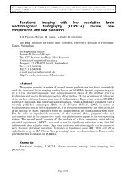
The world of biomedical engineeringBiomechanicsMedical &biological analysisBiosensorsProsthetic devices& artificial organsMedical imagingClinicalengineeringMedical &bioinformaticsBiomaterialsBiotechnologyTissue engineeringRehabilitationengineeringPhysiologicalmodelingBiomedicalinstrumentationNeuralengineeringBionanotechnologyFIGURE 1The World of Biomedical Engineering.• Production of synthetic vaccines from clone cells• Bioenvironmental engineering to protect human, animal, and plant life from toxicants andpollutants• Study of protein–surface interactions• Modeling of the growth kinetics of yeast and hybridoma cells• Research in immobilized enzyme technology• Development of therapeutic proteins and monoclonal antibodiesBiomedical engineers, on the other hand, apply electrical, mechanical, chemical, optical, and otherengineering principles to understand, modify, or control biologic (i.e., human and animal) systems, aswell as design and manufacture products that can monitor physiologic functions and assist in the diagnosisand treatment of patients. When biomedical engineers work within a hospital or clinic, they are moreproperly called clinical engineers.Activities of Biomedical EngineersThe breadth of activity of biomedical engineers is now significant. The field has moved from beingconcerned primarily with the development of medical instruments in the 1950s and 1960s to include amore wide-ranging set of activities. As illustrated below, the field of biomedical engineering now includesmany new career areas (see Figure 1), each of which is presented in this handbook. These areas include:• Application of engineering system analysis (physiologic modeling, simulation, and control) tobiologic problems• Detection, measurement, and monitoring of physiologic signals (i.e., biosensors and biomedicalinstrumentation)• Diagnostic interpretation via signal-processing techniques of bioelectric data• Therapeutic and rehabilitation procedures and devices (rehabilitation engineering)• Devices for replacement or augmentation of bodily functions (artificial organs)

• Computer analysis of patient-related data and clinical decision making (i.e., medical informaticsand artificial intelligence)• Medical imaging, that is, the graphic display of anatomic detail or physiologic function• The creation of new biologic products (i.e., biotechnology and tissue engineering)• The development of new materials to be used within the body (biomaterials)Typical pursuits of biomedical engineers, therefore, include:• Research in new materials for implanted artificial organs• Development of new diagnostic instruments for blood analysis• Computer modeling of the function of the human heart• Writing software for analysis of medical research data• Analysis of medical device hazards for safety and efficacy• Development of new diagnostic imaging systems• Design of telemetry systems for patient monitoring• Design of biomedical sensors for measurement of human physiologic systems variables• Development of expert systems for diagnosis of disease• Design of closed-loop control systems for drug administration• Modeling of the physiological systems of the human body• Design of instrumentation for sports medicine• Development of new dental materials• Design of communication aids for the handicapped• Study of pulmonary fluid dynamics• Study of the biomechanics of the human body• Development of material to be used as replacement for human skinBiomedical engineering, then, is an interdisciplinary branch of engineering that ranges from theoretical,nonexperimental undertakings to state-of-the-art applications. It can encompass research, development,implementation, and operation. Accordingly, like medical practice itself, it is unlikely that any singleperson can acquire expertise that encompasses the entire field. Yet, because of the interdisciplinary natureof this activity, there is considerable interplay and overlapping of interest and effort between them.For example, biomedical engineers engaged in the development of biosensors may interact with thoseinterested in prosthetic devices to develop a means to detect and use the same bioelectric signal to powera prosthetic device. Those engaged in automating the clinical chemistry laboratory may collaborate withthose developing expert systems to assist clinicians in making decisions based on specific laboratory data.The possibilities are endless.Perhaps a greater potential benefit occurring from the use of biomedical engineering is identificationof the problems and needs of our present health care system that can be solved using existing engineeringtechnology and systems methodology. Consequently, the field of biomedical engineering offers hope inthe continuing battle to provide high-quality care at a reasonable cost. If properly directed toward solvingproblems related to preventive medical approaches, ambulatory care services, and the like, biomedicalengineers can provide the tools and techniques to make our health care system more effective and efficient;and in the process, improve the quality of life for all.Joseph D. BronzinoEditor-in-Chief

Editor-in-ChiefJoseph D. Bronzino received the B.S.E.E. degree from Worcester Polytechnic Institute, Worcester, MA,in 1959, the M.S.E.E. degree from the Naval Postgraduate School, Monterey, CA, in 1961, and the Ph.D.degree in electrical engineering from Worcester Polytechnic Institute in 1968. He is presently the VernonRoosa Professor of Applied Science, an endowed chair at Trinity College, Hartford, CT and Presidentof the Biomedical Engineering Alliance and Consortium (BEACON) which is a nonprofit organizationconsisting of academic and medical institutions as well as corporations dedicated to the development andcommercialization of new medical technologies (for details visit www.beaconalliance.org).He is the author of over 200 articles and 11 books including the following: Technology for PatientCare (C.V. Mosby, 1977), Computer Applications for Patient Care (Addison-Wesley, 1982), BiomedicalEngineering: Basic Concepts and Instrumentation (PWS Publishing Co., 1986), Expert Systems: Basic Concepts(Research Foundation of State University of New York, 1989), Medical Technology and Society: AnInterdisciplinary Perspective (MIT Press and McGraw-Hill, 1990), Management of Medical Technology (Butterworth/Heinemann,1992), The Biomedical Engineering Handbook (CRC Press, 1st ed., 1995; 2nd ed.,2000; Taylor & Francis, 3rd ed., 2005), Introduction to Biomedical Engineering (Academic Press, 1st ed.,1999; 2nd ed., 2005).Dr. Bronzino is a fellow of IEEE and the American Institute of Medical and Biological Engineering(AIMBE), an honorary member of the Italian Society of Experimental Biology, past chairman of theBiomedical Engineering Division of the American Society for Engineering Education (ASEE), a chartermember and presently vice president of the Connecticut Academy of Science and Engineering (CASE),a charter member of the American College of Clinical Engineering (ACCE) and the Association for theAdvancement of Medical Instrumentation (AAMI), past president of the IEEE-Engineering in Medicineand Biology Society (EMBS), past chairman of the IEEE Health Care Engineering Policy Committee(HCEPC), past chairman of the IEEE Technical Policy Council in Washington, DC, and presently Editorin-Chiefof Elsevier’s BME Book Series and Taylor & Francis’ Biomedical Engineering Handbook.Dr. Bronzino is also the recipient of the Millennium Award from IEEE/EMBS in 2000 and the GoddardAward from Worcester Polytechnic Institute for Professional Achievement in June 2004.

ContributorsJoseph AdamPremise DevelopmentCorporationHartford, ConnecticutP.D. AhlgrenVille Marie MultidisciplinaryBreast and Oncology CenterSt. Mary’s HospitalMcGill UniversityMontreal, Quebec, CanadaandLondon Cancer CentreLondon, OntarioCanadaWilliam C. AmaluPacific Chiropractic andResearch CenterRedwood City, CaliforniaKurt AmmerLudwig Boltzmann ResearchInstitute for PhysicalDiagnosticsVienna, AustriaandMedical Imaging Research GroupSchool of ComputingUniversity of GlamorganPontypridd, WalesUnited KingdomDennis D. AutioDybonics, Inc.Portland, OregonRaymond BalcerakDefense Advanced ResearchProjects AgencyArlington, VirginiaD.C. BarberUniversity of SheffieldSheffield, United KingdomKhosrow BehbehaniThe University of Texas atArlingtonArlington, TexasandThe University of TexasSouthwestern Medical CenterDallas, TexasN. BelliveauVille Marie MultidisciplinaryBreast and Oncology CenterSt. Mary’s HospitalMcGill UniversityMontreal, Quebec, CanadaandLondon Cancer CentreLondon, Ontario, CanadaAnna M. BianchiSt. Raffaele HospitalMilan, ItalyCarolJ.BickfordAmerican Nurses AssociationWashington, D.C.Jeffrey S. BlairIBM Health Care SolutionsAtlanta, GeorgiaG. Faye Boudreaux-BartelsUniversity of Rhode IslandKingston, Rhode IslandBruce R. BowmanEdenTec CorporationEden Prairie, MinnesotaJoseph D. BronzinoTrinity CollegeBiomedical Engineering Allianceand Consortium (BEACON)Harford, ConnecticutMark E. BruleyECRIPlymouth Meeting, PennsylvaniaRichard P. BuckUniversity of North CarolinaChapel Hill, North CarolinaP. BuddharajuDepartment of Computer ScienceUniversity of HoustonHouston, TexasThomas F. BudingerUniversity of California-BerkeleyBerkeley, CaliforniaRobert D. ButterfieldIVAC CorporationSan Diego, CaliforniaJoseph P. CammarotaNaval Air Warfare CenterAircraft DivisionWarminster, Pennsylvania

Paul CampbellInstitute of Medical Scienceand TechnologyUniversities of St. Andrewsand DundeeandNinewells HospitalDundee, United KingdomEwart R. CarsonCity UniversityLondon, United KingdomSergio CeruttiPolytechnic UniversityMilan, ItalyA. Enis ÇetinBilkent UniversityAnkara, TurkeyChristopher S. ChenDepartment of BioengineeringDepartment of PhysiologyUniversity of PennsylvaniaPhiladelphia, PennsylvaniaWei ChenCenter for Magnetic ResonanceResearchandThe University of MinnesotaMedical SchoolMinneapolis, MinnesotaVictor ChernomordikLaboratory of Integrative andMedical BiophysicsNational Institute of Child Healthand Human DevelopmentBethesda, MarylandDavid A. CheslerMassachusetts General HospitalHarvard University MedicalSchoolBoston, MassachusettsVivian H. CoatesECRIPlymouth Meeting, PennsylvaniaArnon CohenBen-Gurion UniversityBe’er Sheva, IsraelSteven ConollyStanford UniversityStanford, CaliforniaDerek G. CrampCity UniversityLondon, United KingdomBarbara Y. CroftNational Institutes of HealthKensington, MarylandDavid D. CunninghamAbbott DiagnosticsProcess EngineeringAbbott Park, IllinoisIan A. CunninghamVictoria HospitalThe John P. Roberts ResearchInstituteandThe University of Western OntarioLondon, Ontario, CanadaYadin DavidTexas Children’s HospitalHouston, TexasConnie White DelaneySchool of Nursing and MedicalSchoolThe University of MinnesotaMinneapolis, MinnesotaMary DiakidesAdvanced Concepts Analysis, Inc.Falls Church, VirginiaNicholas A. DiakidesAdvanced Concepts Analysis, Inc.Falls Church, VirginiaC. Drews-PeszynskiTechnical University of LodzLodz, PolandRonald G. DriggersU.S. Army Communications andElectronics Research,Development and EngineeringCenter (CERDEC)Night Vision and ElectronicSensors DirectorateFort Belvoir, VirginiaGary DrzewieckiRutgers UniversityPiscataway, New JerseyEdwin G. DuffinMedtronic, Inc.Minneapolis, MinnesotaJeffrey L. EgglestonValleylab, Inc.Boulder, ColoradoRobert L. ElliottElliott-Elliott-Head Breast CancerResearch and Treatment CenterBaton Rouge, LouisianaK. Whittaker FerraraRiverside Research InstituteNew York, New YorkJ. Michael FitzmauriceAgency for Healthcare Researchand QualityRockville, MarylandRoss FlewellingNellcor IncorporationPleasant, CaliforniaMichael FordeMedtronic, Inc.Minneapolis, MinnesotaAmir H. GandjbakhcheLaboratory of Integrative andMedical BiophysicsNational Institute of Child Healthand Human DevelopmentBethesda, MarylandIsrael GannotLaboratory of Integrative andMedical BiophysicsNational Institute of Child Healthand Human DevelopmentBethesda, MarylandLeslie A. GeddesPurdue UniversityWest Lafayette, IndianaRichard L. GoldbergUniversity of North CarolinaChapel Hill, North Carolina

Boris GramatikovJohns Hopkins Schoolof MedicineBaltimore, MarylandBarton M. GrattSchool of DentistryUniversity of WashingtonSeattle, WashingtonWalter GreenleafGreenleaf MedicalPalo Alto, CaliforniaMichael W. GrennU.S. Army Communications andElectronics Research,Development and EngineeringCenter (CERDEC)Night Vision and ElectronicSensors DirectorateFort Belvoir, VirginiaEliot B. GriggDepartment of Plastic SurgeryDartmouth-Hitchcock MedicalCenterLebanon, New HampshireWarren S. GrundfestDepartment of Bioengineeringand Electrical EngineeringHenry Samueli School ofEngineering and AppliedScienceandDepartment of SurgeryDavid Geffen Schoolof MedicineUniversity of CaliforniaLos Angeles, CaliforniaMichael L. GulliksonTexas Children’s HospitalHouston, TexasMoinuddin HassanLaboratory of Integrative andMedical BiophysicsNational Institute of Child Healthand Human DevelopmentBethesda, MarylandDavid HatteryLaboratory of Integrative andMedical BiophysicsNational Institute of Child Healthand Human DevelopmentBethesda, MarylandJonathan F. HeadElliott-Elliott-Head Breast CancerResearch and Treatment CenterBaton Rouge, LouisianaWilliam B. HobbinsWomen’s Breast Health CenterMadison, WisconsinStuart HornU.S. Army Communications andElectronics Research,Development and EngineeringCenter (CERDEC)Night Vision and ElectronicSensors DirectorateFort Belvoir, VirginiaXiaoping HuCenter for Magnetic ResonanceResearchandThe University of MinnesotaMedical SchoolMinneapolis, MinnesotaT. JakubowskaTechnical University of LodzLodz, PolandG. Allan JohnsonDuke University Medical CenterDurham, North CarolinaBryan F. JonesMedical Imaging Research GroupSchool of ComputingUniversity of GlamorganPontypridd, WalesUnited KingdomThomas M. JuddKaiser PermanenteAtlanta, GeorgiaMillard M. JudyBaylor Research Institute andMicroBioMed Corp.Dallas, TexasPhilip F. JudyBrigham and Women’s HospitalHarvard University MedicalSchoolBoston, MassachusettsG.J.L. KawDepartment of DiagnosticRadiologyTan Tock Seng HospitalSingaporeJ.R. KeyserlingkVille Marie MultidisciplinaryBreast and Oncology CenterSt. Mary’s HospitalMcGill UniversityMontreal, Quebec, CanadaandLondon Cancer CentreLondon, OntarioCanadaC. Everett KoopDepartment of Plastic SurgeryDartmouth-Hitchcock MedicalCenterLebanon, New HampshireHayrettin KöymenBilkent UniversityAnkara, TurkeyLuis G. KunIRMC/National DefenseUniversityWashington, D.C.Phani Teja KurugantiRF and Microwave Systems GroupOak Ridge National LaboratoryOak Ridge, TennesseeKenneth K. KwongMassachusetts General HospitalHarvard University MedicalSchoolBoston, Massachusetts

Z.R. LiSouth China Normal UniversityGuangzhou, ChinaRichard F. LittleNational Institutes of HealthBethesda, MarylandChung-Chiun LiuElectronics Design Center andEdison Sensor TechnologyCenterCase Western Reserve UniversityCleveland, OhioZhongqi LiuTTM Management GroupBeijing, ChinaJasper LupoApplied Research Associates, Inc.Falls Church, VirginiaAlbert MacovskiStanford UniversityStanford, CaliforniaLuca T. MainardiPolytechnic UniversityMilan, ItalyC. ManoharDepartment of Electrical &Computer EngineeringUniversity of HoustonHouston, TexasJoseph P. McClainWalter Reed Army Medical CenterWashington, D.C.Kathleen A. McCormickSAICFalls Church, VirginiaDennis McGrathDepartment of Plastic SurgeryDartmouth-Hitchcock MedicalCenterLebanon, New HampshireSusan McGrathDepartment of Plastic SurgeryDartmouth-Hitchcock MedicalCenterLebanon, New HampshireMatthew F. McKnightDepartment of Plastic SurgeryDartmouth-Hitchcock MedicalCenterLebanon, New HampshireYitzhak MendelsonWorcester Polytechnic InstituteWorcester, MassachusettsJames B. MercerUniversity of TromsøTromsø, NorwayArcangelo MerlaDepartment of Clinical Sciencesand BioimagingUniversity “G.d’Annunzio”andInstitute for Advanced BiomedicalTechnologyFoundation “G.d’Annunzio”andIstituto Nazionale Fisica dellaMateriaCoordinated Group of ChietiChieti-Pescara, ItalyEvangelia Micheli-TzanakouRutgers UnversityPiscataway, New JerseyRobert L. MorrisDybonics, Inc.Portland, OregonJack G. MottleyUniversity of RochesterRochester, New YorkRobin MurrayUniversity of Rhode IslandKingston, Rhode IslandJoachim H. NagelUniversity of StuttgartStuttgart, GermanyMichael R. NeumanMichigan TechnologicalUniversityHoughton, MichiganE.Y.K. NgCollege of EngineeringSchool of Mechanical andProduction EngineeringNanyang Technological UniversitySingaporePaul NortonU.S. Army Communications andElectronics Research,Development and EngineeringCenter (CERDEC)Night Vision and ElectronicSensors DirectorateFort Belvoir, VirginiaAntoni NowakowskiDepartment of BiomedicalEngineering,Gdansk University of TechnologyNarutowiczaGdansk, PolandBanu OnaralDrexel UniversityPhiladelphia, PennsylvaniaDavid D. PascoeAuburn UniversityAuburn, AlabamaMaqbool PatelCenter for Magnetic ResonanceResearchandThe University of MinnesotaMedical SchoolMinneapolis, MinnesotaRobert PattersonThe University of MinnesotaMinneapolis, MinnesotaJeffrey L. PaulDefense Advanced ResearchProjects AgencyArlington, VirginiaA. William PaulsenEmory UniversityAtlanta, Georgia

John PaulyStanford UniversityStanford, CaliforniaI. PavlidisDepartment of Computer ScienceUniversity of HoustonHouston, TexasP. Hunter PeckhamCase Western Reserve UniversityCleveland, OhioJoseph G. PellegrinoU.S. Army Communications andElectronics Research,Development and EngineeringCenter (CERDEC)Night Vision and ElectronicSensors DirectorateFort Belvoir, VirginiaPhilip PercontiU.S. Army Communications andElectronics Research,Development and EngineeringCenter (CERDEC)Night Vision and ElectronicSensors DirectorateFort Belvoir, VirginiaAthina P. PetropuluDrexel UniversityPhiladelphia, PennsylvaniaTom PiantanidaGreenleaf MedicalPalo Alto, CaliforniaT. Allan PryorUniversity of UtahSalt Lake City, UtahRam C. PurohitAuburn UniversityAuburn, AlabamaHairong QiECE DepartmentThe University of TennesseeKnoxville, TennesseePat RidgelyMedtronic, Inc.Minneapolis, MinnesotaE. Francis RingMedical Imaging Research GroupSchool of ComputingUniversity of GlamorganPontypridd, WalesUnited KingdomRichardL.RoaBaylor University Medical CenterDallas, TexasPeter RobbieDepartment of Plastic SurgeryDartmouth-Hitchcock MedicalCenterLebanon, New HampshireGian Luca RomaniDepartment of Clinical Sciencesand BioimagingUniversity “G. d’Annunzio”andInstitute for AdvancedBiomedical TechnologyFoundation “G.d’Annunzio”andIstituto Nazionale Fisica dellaMateriaCoordinated Group of ChietiChieti-Pescara, ItalyJoseph M. RosenDepartment of Plastic SurgeryDartmouth-Hitchcock MedicalCenterLebanon, New HampshireEric RosowHartford HospitalandPremise DevelopmentCorporationHartford, ConnecticutSubrata SahaClemson UniversityClemson, South CarolinaJohn SchenckGeneral Electric CorporateResearch and DevelopmentCenterSchenectady, New YorkEdward SchuckEdenTec CorporationEden Prairie, MinnesotaJoyce SensmeierHIMSSChicago, IllinoisDavid ShermanJohns Hopkins School of MedicineBaltimore, MarylandRobert E. Shroy, Jr.Picker InternationalHighland Heights, OhioStephen W. SmithDuke UniversityDurham, North CarolinaNathan J. SniadeckiDepartment of BioengineeringUniversity of PennsylvaniaPhiladelphia, PennsylvaniaWesley E. SnyderECE DepartmentNorth Carolina State UniversityRaleigh, North CarolinaOrhan SoykanCorporate Science andTechnologyMedtronic, Inc.andDepartment of BiomedicalEngineeringMichigan TechnologicalUniversityHoughton, MichiganPrimoz StrojnikCase Western Reserve UniversityCleveland, OhioM. StrzeleckiTechnical University of LodzLodz, PolandRon SummersLoughborough UniversityLeicestershire, United KingdomChristopher SwiftDepartment of Plastic SurgeryDartmouth-Hitchcock MedicalCenterLebanon, New HampshireWillis A. TackerPurdue UniversityWest Lafayette, Indiana

Nitish V. ThakorJohns Hopkins School of MedicineBaltimore, MarylandRoderick ThomasFaculty of Applied Design andEngineeringSwansea Institute of TechnologySwansea, United KingdomP. TsiamyrtzisDepartment of StatisticsUniversity of Economics andBusiness AthensAthens, GreeceBenjamin M.W. TsuiUniversity of North CarolinaChapel Hill, North CarolinaTracy A. TurnerPrivate PracticeMinneapolis, MinnesotaKamil UgurbilCenter for Magnetic ResonanceResearchandThe University of MinnesotaMedical SchoolMinneapolis, MinnesotaMichael S. Van LyselUniversity of WisconsinMadison, WisconsinHenry F. VanBrocklinUniversity of California-BerkeleyBerkeley, CaliforniaJay VizgaitisU.S. Army Communications andElectronics Research,Development and EngineeringCenter (CERDEC)Night Vision and ElectronicSensors DirectorateFort Belvoir, VirginiaAbby VogelLaboratory of Integrative andMedical BiophysicsNational Institute of Child Healthand Human DevelopmentBethesda, MarylandWolf W. von MaltzahnRensselaer Polytechnic InstituteTroy, New YorkGregory I. VossIVAC CorporationSan Diego, CaliforniaAlvin WaldColumbia UniversityNew York, New YorkChen WangTTM InternationalHouston, TexasLois de WeerdUniversity Hospital ofNorth NorwayTromsø, NorwayWang WeiRadiology DepartmentBeijing You An HospitalBeijing, ChinaB. WiecekTechnical University of LodzLodz, PolandM. WysockiTechnical University of LodzLodz, PolandMartin J. YaffeUniversity of TorontoToronto, Ontario, CanadaRobert YarchoanHIV and AIDS MalignancyBranchCenter for Cancer ResearchNational Cancer Institute (NCI)Bethesda, MarylandM. YassaVille Marie MultidisciplinaryBreast and Oncology CenterSt. Mary’s HospitalMcGill UniversityMontreal, Quebec, CanadaandLondon Cancer CentreLondon, Ontario, CanadaChristopher M. YipDepartments of ChemicalEngineering and AppliedChemistryDepartment of BiochemistryInstitute of Biomaterials andBiomedical EngineeringUniversity of TorontoToronto, Ontario, CanadaE. YuVille Marie MultidisciplinaryBreast and Oncology CenterSt. Mary’s HospitalMcGill UniversityMontreal, Quebec, CanadaandLondon Cancer CentreLondon, Ontario, CanadaWen YuShanghai RuiJin HospitalShanghai, ChinaYune YuanInstitute of Basic Medical ScienceChina Army General HospitalBeijing, ChinaJason ZeibelU.S. Army Communications andElectronics Research,Development and EngineeringCenter (CERDEC)Night Vision and ElectronicSensors DirectorateFort Belvoir, VirginiaYi ZengCentral Disease Control of ChinaBeijing, ChinaXiaohong ZhouDuke University Medical CenterDurham, North CarolinaYulin ZhouShanghai RuiJin HospitalShanghai, China

ContentsSECTIONIBiomedical Signal AnalysisBanu Onaral1 Biomedical Signals: Origin and Dynamic Characteristics;Frequency-Domain AnalysisArnon Cohen . . . . . . . . . . . . . . . . . . . . . 1-12 Digital Biomedical Signal Acquisition and ProcessingLuca T. Mainardi, Anna M. Bianchi, Sergio Cerutti . . . . 2-13 Compression of Digital Biomedical SignalsA. Enis Çetin, Hayrettin Köymen . . . . . . . . . . . . 3-14 Time-Frequency Signal Representations forBiomedical SignalsG. Faye Boudreaux-Bartels, Robin Murray . . . . . . . . 4-15 Wavelet (Time-Scale) Analysis in BiomedicalSignal ProcessingNitish V. Thakor, Boris Gramatikov, David Sherman . . . 5-16 Higher-Order Spectral AnalysisAthina P. Petropulu . . . . . . . . . . . . . . . . . . 6-17 Neural Networks in Biomedical Signal ProcessingEvangelia Micheli-Tzanakou . . . . . . . . . . . . . . 7-18 Complexity, Scaling, and Fractals in Biomedical SignalsBanu Onaral, Joseph P. Cammarota . . . . . . . . . . . 8-19 Future Directions: Biomedical Signal Processing andNetworked Multimedia CommunicationsBanu Onaral . . . . . . . . . . . . . . . . . . . . . 9-1

SECTIONIIImagingWarren S. Grundfest10 X-RayRobert E. Shroy, Jr., Michael S. Van Lysel,Martin J. Yaffe . . . . . . . . . . . . . . . . . . . . 10-111 Computed TomographyIan A. Cunningham, Philip F. Judy . . . . . . . . . . . 11-112 Magnetic Resonance ImagingSteven Conolly, Albert Macovski, John Pauly, John Schenck,Kenneth K. Kwong, David A. Chesler, Xiaoping Hu,Wei Chen, Maqbool Patel, Kamil Ugurbil . . . . . . . . 12-113 Nuclear MedicineBarbara Y. Croft, Benjamin M.W. Tsui . . . . . . . . . . 13-114 UltrasoundRichard L. Goldberg, Stephen W. Smith, Jack G. Mottley,K. Whittaker Ferrara . . . . . . . . . . . . . . . . . 14-115 Magnetic Resonance MicroscopyXiaohong Zhou, G. Allan Johnson . . . . . . . . . . . . 15-116 Positron-Emission Tomography (PET)Thomas F. Budinger, Henry F. VanBrocklin . . . . . . . . 16-117 Electrical Impedance TomographyD.C. Barber . . . . . . . . . . . . . . . . . . . . . 17-118 Medical Applications of Virtual Reality TechnologyWalter Greenleaf, Tom Piantanida . . . . . . . . . . . 18-1SECTIONIIIInfrared ImagingNicholas A. Diakides19 Advances in Medical Infrared ImagingNicholas Diakides, Mary Diakides, Jasper Lupo,Jeffrey L. Paul, Raymond Balcerak . . . . . . . . . . . 19-120 The Historical Development of Thermometryand Thermal Imaging in MedicineE. Francis Ring, Bryan F. Jones . . . . . . . . . . . . . 20-1

21 Physiology of Thermal SignalsDavid D. Pascoe, James B. Mercer, Lois de Weerd . . . . . 21-122 Quantitative Active Dynamic Thermal IR-Imaging andThermal Tomography in Medical DiagnosticsAntoni Nowakowski . . . . . . . . . . . . . . . . . 22-123 Thermal Texture Maps (TTM): Concept, Theory, andApplicationsZhongqi Liu, Chen Wang, Hairong Qi, Yune Yuan, Yi Zeng,Z.R. Li, Yulin Zhou, Wen Yu, Wang Wei . . . . . . . . . 23-124 IR Imagers as Fever Monitoring Devices: Physics,Physiology, and Clinical AccuracyE.Y.K. Ng, G.J.L. Kaw . . . . . . . . . . . . . . . . . 24-125 Infrared Imaging of the Breast — An OverviewWilliam C. Amalu, William B. Hobbins, Jonathan F. Head,Robert L. Elliott . . . . . . . . . . . . . . . . . . . 25-126 Functional Infrared Imaging of the Breast:Historical Perspectives, Current Application, andFuture ConsiderationsJ.R. Keyserlingk, P.D. Ahlgren, E. Yu, N. Belliveau,M. Yassa . . . . . . . . . . . . . . . . . . . . . . . 26-127 Detecting Breast Cancer from Thermal Infrared Images byAsymmetry AnalysisHairong Qi, Phani Teja Kuruganti, Wesley E. Snyder . . . 27-128 Advanced Thermal Image ProcessingB. Wiecek, M. Strzelecki, T. Jakubowska, M. Wysocki,C. Drews-Peszynski . . . . . . . . . . . . . . . . . . 28-129 Biometrics: Face Recognition in Thermal InfraredI. Pavlidis, P. Tsiamyrtzis, P. Buddharaju, C. Manohar . . . 29-130 Infrared Imaging for Tissue Characterization and FunctionMoinuddin Hassan, Victor Chernomordik, Abby Vogel,David Hattery, Israel Gannot, Richard F. Little,Robert Yarchoan, Amir H. Gandjbakhche . . . . . . . . 30-131 Thermal Imaging in Diseases of the Skeletal andNeuromuscular SystemsE. Francis Ring, Kurt Ammer . . . . . . . . . . . . . . 31-132 Functional Infrared Imaging in Clinical ApplicationsArcangelo Merla, Gian Luca Romani . . . . . . . . . . 32-1

33 Thermal Imaging in SurgeryPaul Campbell, Roderick Thomas . . . . . . . . . . . . 33-134 Infrared Imaging Applied to DentistryBarton M. Gratt . . . . . . . . . . . . . . . . . . . 34-135 Use of Infrared Imaging in Veterinary MedicineRam C. Purohit, Tracy A. Turner, David D. Pascoe . . . . 35-136 Standard Procedures for Infrared Imaging in MedicineKurt Ammer, E. Francis Ring . . . . . . . . . . . . . . 36-137 Infrared Detectors and Detector ArraysPaul Norton, Stuart Horn, Joseph G. Pellegrino,Philip Perconti . . . . . . . . . . . . . . . . . . . . 37-138 Infrared Camera CharacterizationJoseph G. Pellegrino, Jason Zeibel, Ronald G. Driggers,Philip Perconti . . . . . . . . . . . . . . . . . . . . 38-139 Infrared Camera and Optics for Medical ApplicationsMichael W. Grenn, Jay Vizgaitis, Joseph G. Pellegrino,Philip Perconti . . . . . . . . . . . . . . . . . . . . 39-1SECTIONIVMedical InformaticsLuis G. Kun40 Hospital Information Systems: Their Function and StateT. Allan Pryor . . . . . . . . . . . . . . . . . . . . 40-141 Computer-Based Patient RecordsJ. Michael Fitzmaurice . . . . . . . . . . . . . . . . . 41-142 Overview of Standards Related to the Emerging Health CareInformation InfrastructureJeffrey S. Blair . . . . . . . . . . . . . . . . . . . . 42-143 Introduction to Informatics and NursingKathleen A. McCormick, Joyce Sensmeier,Connie White Delaney, Carol J. Bickford . . . . . . . . . 43-144 Non-AI Decision MakingRon Summers, Derek G. Cramp, Ewart R. Carson . . . . . 44-1

45 Medical Informatics and Biomedical Emergencies: NewTraining and Simulation Technologies for First RespondersJoseph M. Rosen, Christopher Swift, Eliot B. Grigg,Matthew F. McKnight, Susan McGrath, Dennis McGrath,Peter Robbie, C. Everett Koop . . . . . . . . . . . . . 45-1SECTIONVBiomedical SensorsMichael R. Neuman46 Physical MeasurementsMichael R. Neuman . . . . . . . . . . . . . . . . . . 46-147 Biopotential ElectrodesMichael R. Neuman . . . . . . . . . . . . . . . . . . 47-148 Electrochemical SensorsChung-Chiun Liu . . . . . . . . . . . . . . . . . . . 48-149 Optical SensorsYitzhak Mendelson . . . . . . . . . . . . . . . . . . 49-150 Bioanalytic SensorsRichard P. Buck . . . . . . . . . . . . . . . . . . . 50-151 Biological Sensors for DiagnosticsOrhan Soykan . . . . . . . . . . . . . . . . . . . . 51-1SECTIONVIMedical Instruments and DevicesWolf W. von Maltzahn52 Biopotential AmplifiersJoachim H. Nagel . . . . . . . . . . . . . . . . . . . 52-153 Bioelectric Impedance MeasurementsRobert Patterson . . . . . . . . . . . . . . . . . . . 53-154 Implantable Cardiac PacemakersMichael Forde, Pat Ridgely . . . . . . . . . . . . . . . 54-155 Noninvasive Arterial Blood Pressure and MechanicsGary Drzewiecki . . . . . . . . . . . . . . . . . . . 55-1

56 Cardiac Output MeasurementLeslie A. Geddes . . . . . . . . . . . . . . . . . . . 56-157 External DefibrillatorsWillis A. Tacker . . . . . . . . . . . . . . . . . . . 57-158 Implantable DefibrillatorsEdwin G. Duffin . . . . . . . . . . . . . . . . . . . 58-159 Implantable Stimulators for Neuromuscular ControlPrimoz Strojnik, P. Hunter Peckham . . . . . . . . . . 59-160 RespirationLeslie A. Geddes . . . . . . . . . . . . . . . . . . . 60-161 Mechanical VentilationKhosrow Behbehani . . . . . . . . . . . . . . . . . . 61-162 Essentials of Anesthesia DeliveryA. William Paulsen . . . . . . . . . . . . . . . . . . 62-163 Electrosurgical DevicesJeffrey L. Eggleston, Wolf W. von Maltzahn . . . . . . . . 63-164 Biomedical LasersMillard M. Judy . . . . . . . . . . . . . . . . . . . . 64-165 Instrumentation for Cell MechanicsNathan J. Sniadecki, Christopher S. Chen . . . . . . . . 65-166 Blood Glucose MonitoringDavid D. Cunningham . . . . . . . . . . . . . . . . 66-167 Atomic Force Microscopy: Probing BiomolecularInteractionsChristopher M. Yip . . . . . . . . . . . . . . . . . . 67-168 Parenteral Infusion DevicesGregory I. Voss, Robert D. Butterfield . . . . . . . . . . 68-169 Clinical Laboratory: Separation and Spectral MethodsRichard L. Roa . . . . . . . . . . . . . . . . . . . . 69-170 Clinical Laboratory: Nonspectral Methods and AutomationRichard L. Roa . . . . . . . . . . . . . . . . . . . . 70-171 Noninvasive Optical MonitoringRoss Flewelling . . . . . . . . . . . . . . . . . . . . 71-1

72 Medical Instruments and Devices Used in the HomeBruce R. Bowman, Edward Schuck . . . . . . . . . . . 72-173 Virtual Instrumentation: Applications in BiomedicalEngineeringEric Rosow, Joseph Adam . . . . . . . . . . . . . . . 73-1SECTIONVIIClinical EngineeringYadin David74 Clinical Engineering: Evolution of a DisciplineJoseph D. Bronzino . . . . . . . . . . . . . . . . . . 74-175 Management and Assessment of Medical TechnologyYadin David, Thomas M. Judd . . . . . . . . . . . . . 75-176 Risk Factors, Safety, and Management of Medical EquipmentMichael L. Gullikson . . . . . . . . . . . . . . . . . 76-177 Clinical Engineering Program IndicatorsDennis D. Autio, Robert L. Morris . . . . . . . . . . . . 77-178 Quality of Improvement and Team BuildingJoseph P. McClain . . . . . . . . . . . . . . . . . . . 78-179 A Standards Primer for Clinical EngineersAlvin Wald . . . . . . . . . . . . . . . . . . . . . 79-180 Regulatory and Assessment AgenciesMark E. Bruley, Vivian H. Coates . . . . . . . . . . . . 80-181 Applications of Virtual Instruments in Health CareEric Rosow, Joseph Adam . . . . . . . . . . . . . . . 81-1SECTIONVIII Ethical Issues Associated withthe Use of Medical TechnologySubrata Saha and Joseph D. Bronzino82 Beneficence, Nonmaleficence, and Medical TechnologyJoseph D. Bronzino . . . . . . . . . . . . . . . . . . 82-183 Ethical Issues Related to Clinical ResearchJoseph D. Bronzino . . . . . . . . . . . . . . . . . . 83-1Index . . . . . . . . . . . . . . . . . . . . . . . . . . . . . I-1

IBiomedical SignalAnalysisBanu OnaralDrexel University1 Biomedical Signals: Origin and Dynamic Characteristics;Frequency-Domain AnalysisArnon Cohen ......................................... 1-12 Digital Biomedical Signal Acquisition and ProcessingLuca T. Mainardi, Sergio Cerutti, Anna M. Bianchi .................... 2-13 Compression of Digital Biomedical SignalsA. Enis Çetin, Hayrettin Köymen .............................. 3-14 Time–Frequency Signal Representations for Biomedical SignalsG. Faye Boudreaux-Bartels, Robin Murray ......................... 4-15 Wavelet (Time-Scale) Analysis in Biomedical Signal ProcessingNitish V. Thakor, Boris Gramatikov, David Sherman ................... 5-16 Higher-Order Spectral AnalysisAthina P. Petropulu ...................................... 6-17 Neural Networks in Biomedical Signal ProcessingEvangelia Micheli-Tzanakou ................................. 7-18 Complexity, Scaling, and Fractals in Biomedical SignalsBanu Onaral, Joseph P. Cammarota ............................ 8-1I-1

I-2 Medical Devices and Systems9 Future Directions: Biomedical Signal Processing and NetworkedMultimedia CommunicationsBanu Onaral ......................................... 9-1BIOMEDICAL SIGNAL ANALYSIS CENTERS on the acquisition and processing of informationbearingsignals that emanate from living systems. These vital signals permit us to probe the state ofthe underlying biologic and physiologic structures and dynamics. Therefore, their interpretationhas significant diagnostic value for clinicians and researchers.The detected signals are commonly corrupted with noise. Often, the information cannot be readilyextracted from the raw signal, which must be processed in order to yield useful results. Signals and systemsengineering knowledge and, in particular, signal-processing expertise are therefore critical in all phases ofsignal collection and analysis.Biomedical engineers are called on to conceive and implement processing schemes suitable for biomedicalsignals. They also play a key role in the design and development of biomedical monitoring devicesand systems that match advances in signal processing and instrumentation technologies with biomedicalneeds and requirements.This section is organized in two main parts. In the first part, contributing authors review contemporarymethods in biomedical signal processing. The second part is devoted to emerging methods that hold thepromise for major enhancements in our ability to extract information from vital signals.The success of signal-processing applications strongly depends on the knowledge about the origin andthe nature of the signal. Biomedical signals possess many special properties and hence require specialtreatment. Also, the need for noninvasive measurements presents unique challenges that demand a clearunderstanding of biomedical signal characteristics. In the lead chapter, entitled, “Biomedical Signals:Origin and Dynamic Characteristics; Frequency-Domain Analysis,” Arnon Cohen provides a generalclassification of biomedical signals and discusses basics of frequency domain methods.The advent of digital computing coupled with fast progress in discrete-time signal processing has led toefficient and flexible methods to acquire and treat biomedical data in digital form. The chapter entitled,“Digital Biomedical Signal Acquisition and Processing,” by Luca T. Mainardi, Anna M. Bianchi, and SergioCerutti, presents basic elements of signal acquisition and processing in the special context of biomedicalsignals.Especially in the case of long-term monitoring, digital biomedical signal-processing applications generatevast amounts of data that strain transmission and storage resources. The creation of multipatientreference signal bases also places severe demands on storage. Data compression methods overcome theseobstacles by eliminating signal redundancies while retaining clinically significant information. A. EnisCetin and Hayrettin Köymen provide a comparative overview of a range of approaches from conventionalto modern compression techniques suitable for biomedical signals. Futuristic applications involving longtermand ambulatory recording systems, and remote diagnosis opportunities will be made possible bybreakthroughs in biomedical data compression. This chapter serves well as a point of departure.Constraints such as stationarity (and time invariance), gaussianity (and minimum phaseness), and theassumption of a characteristic scale in time and space have constituted the basic, and by now implicit,assumptions upon which the conventional signals and systems theories have been founded. However,investigators engaged in the study of biomedical processes have long known that they did not hold undermost realistic situations and hence could not sustain the test of practice.Rejecting or at least relaxing restrictive assumptions always opens new avenues for research and yieldsfruitful results. Liberating forces in signals and systems theories have conspired in recent years to createresearch fronts that target long-standing constraints in the established wisdom (dogma?) of classic signalprocessing and system analysis. The emergence of new fields in signals and system theories that addressthese shortcomings and aim to relax these restrictions has been motivated by scientists who, rather

Biomedical Signal Analysis I-3than mold natural behavior into artificial models, seek methods inherently suited to represent reality.Biomedical scientists and engineers are inspired by insights gained from a deeper appreciation for thedynamic richness displayed by biomedical phenomena; hence, more than their counterparts in otherdisciplines, they more forcefully embrace innovations in signal processing.One of these novel directions is concerned with time–frequency representations tailored for nonstationaryand transient signals. Faye Boudreaux-Bartels and Robin Murray address this issue, provide anintroduction to concepts and tools of time–frequency analysis, and point out candidate applications.Many physiologic structures and dynamics defy the concept of a characteristic spatial and temporalscale and must be dealt with employing methods compatible with their multiscale nature. Judging fromthe recent success of biomedical signal-processing applications based on time-scale analysis and wavelettransforms, the resolution of many outstanding processing issues may be at hand. The chapter entitled,“Time-Scale Analysis and Wavelets in Biomedical Signals,” by Nitish V. Thakor, familiarizes the readerwith fundamental concepts and methods of wavelet analysis and suggests fruitful directions in biomedicalsignal processing.The presence of nonlinearities and statistics that do not comply with the gaussianity assumption andthe desire for phase reconstruction have been the moving forces behind investigations of higher-orderstatistics and polyspectra in signal-processing and system-identification fields. An introduction to thetopic and potential uses in biomedical signal-processing applications are presented by Athina Petropuluin the chapter entitled, “Higher-Order Spectra in Biomedical Signal Processing.”Neural networks derive their cue from biologic systems and, in turn, mimic many of the functions ofthe nervous system. Simple networks can filter, recall, switch, amplify, and recognize patterns and henceserve well many signal-processing purposes. In the chapter entitled, “Neural Networks in BiomedicalSignal Processing,” Evangelia Tzanakou helps the reader explore the power of the approach while stressinghow biomedical signal-processing applications benefit from incorporating neural-network principles.The dichotomy between order and disorder is now perceived as a ubiquitous property inherent in theunfolding of many natural complex phenomena. In the last decade, it has become clear that the commonthreads shared by natural forms and functions are the “physics of disorder” and the “scaling order,” thehallmark of broad classes of fractal entities. Biomedical signals are the global observables of underlyingcomplex physical and physiologic processes. “Complexity” theories therefore hold the potential to providemathematical tools that describe and possibly shed light on the internal workings of physiologic systems.In the next to last chapter in this section, Banu Onaral and Joseph P. Cammarota introduce the readerto basic tenets of complexity theories and the attendant scaling concepts with hopes to facilitate theirintegration into the biomedical engineering practice.The section concludes with a brief chapter on the visions of the future when biomedical signal processingwill merge with the rising technologies in telecommunication and multimedia computing, andeventually with virtual reality, to enable remote monitoring, diagnosis, and intervention. The impact ofthis development on the delivery of health care and the quality of life will no doubt be profound. Thepromise of biomedical signal analysis will then be fulfilled.

1Biomedical Signals:Origin and DynamicCharacteristics;Frequency-DomainAnalysisArnon CohenBen-Gurion University1.1 Origin of Biomedical Signals............................ 1-21.2 Classification of Biosignals .............................. 1-31.3 Stochastic Signals ........................................ 1-51.4 Frequency-Domain Analysis ............................ 1-71.5 Discrete Signals .......................................... 1-91.6 Data Windows............................................ 1-111.7 Short-Time Fourier Transform ......................... 1-121.8 Spectral Estimation ...................................... 1-13The Blackman–Tukey Method • The Periodogram •Time-Series Analysis Methods1.9 Signal Enhancement ..................................... 1-151.10 Optimal Filtering ........................................ 1-16Minimization of Mean Squared Error: The Wiener Filter •Maximization of the Signal-to-Noise Ratio: The MatchedFilter1.11 Adaptive Filtering ........................................ 1-181.12 Segmentation of Nonstationary Signals ................ 1-21References ....................................................... 1-22A signal is a phenomenon that conveys information. Biomedical signals are signals, used in biomedicalfields, mainly for extracting information on a biologic system under investigation. The complete processof information extraction may be as simple as a physician estimating the patient’s mean heart rate byfeeling, with the fingertips, the blood pressure pulse or as complex as analyzing the structure of internalsoft tissues by means of a complex CT machine.Most often in biomedical applications (as in many other applications), the acquisition of the signal isnot sufficient. It is required to process the acquired signal to get the relevant information “buried” in it.1-1

1-2 Medical Devices and SystemsThis may be due to the fact that the signal is noisy and thus must be “cleaned” (or in more professionalterminology, the signal has to be enhanced) or due to the fact that the relevant information is not “visible”in the signal. In the latter case, we usually apply some transformation to enhance the required information.The processing of biomedical signals poses some unique problems. The reason for this is mainly thecomplexity of the underlying system and the need to perform indirect, noninvasive measurements. A largenumber of processing methods and algorithms is available. In order to apply the best method, the usermust know the goal of the processing, the test conditions, and the characteristics of the underlying signal.In this chapter, the characteristics of biomedical signals will be discussed [Cohen, 1986]. Biomedicalsignals will be divided into characteristic classes, requiring different classes of processing methods. Alsoin this chapter, the basics of frequency-domain processing methods will be presented.1.1 Origin of Biomedical SignalsFrom the broad definition of the biomedical signal presented in the preceding section, it is clear thatbiomedical signals differ from other signals only in terms of the application — signals that are used in thebiomedical field. As such, biomedical signals originate from a variety of sources. The following is a briefdescription of these sources:1. Bioelectric signals. The bioelectric signal is unique to biomedical systems. It is generated by nerve cellsand muscle cells. Its source is the membrane potential, which under certain conditions may be excitedto generate an action potential. In single cell measurements, where specific microelectrodes are usedas sensors, the action potential itself is the biomedical signal. In more gross measurements, where, forexample, surface electrodes are used as sensors, the electric field generated by the action of many cells,distributed in the electrode’s vicinity, constitutes the bioelectric signal. Bioelectric signals are probablythe most important biosignals. The fact that most important biosystems use excitable cells makes itpossible to use biosignals to study and monitor the main functions of the systems. The electric fieldpropagates through the biologic medium, and thus the potential may be acquired at relatively convenientlocations on the surface, eliminating the need to invade the system. The bioelectric signal requires arelatively simple transducer for its acquisition. A transducer is needed because the electric conduction inthe biomedical medium is done by means of ions, while the conduction in the measurement system is byelectrons. All these lead to the fact that the bioelectric signal is widely used in most fields of biomedicine.2. Bioimpedance signals. The impedance of the tissue contains important information concerning itscomposition, blood volume, blood distribution, endocrine activity, automatic nervous system activity,and more. The bioimpedance signal is usually generated by injecting into the tissue under test sinusoidalcurrents (frequency range of 50 kHz–1 MHz, with low current densities of the order of 20–20 mA). Thefrequency range is chosen to minimize electrode polarization problems, and the low current densities arechosen to avoid tissue damage mainly due to heating effects. Bioimpedance measurements are usuallyperformed with four electrodes. Two source electrodes are connected to a current source and are usedto inject the current into the tissue. The two measurement electrodes are placed on the tissue underinvestigation and are used to measure the voltage drop generated by the current and the tissue impedance.3. Bioacoustic signals. Many biomedical phenomena create acoustic noise. The measurement of thisacoustic noise provides information about the underlying phenomenon. The flow of blood in the heart,through the heart’s valves, or through blood vessels generates typical acoustic noise. The flow of airthrough the upper and lower airways and in the lungs creates acoustic sounds. These sounds, known ascoughs, snores, and chest and lung sounds, are used extensively in medicine. Sounds are also generatedin the digestive tract and in the joints. It also has been observed that the contracting muscle producesan acoustic noise (muscle noise). Since the acoustic energy propagates through the biologic medium, thebioacoustic signal may be conveniently acquired on the surface, using acoustic transducers (microphonesor accelerometers).4. Biomagnetic signals. Various organs, such as the brain, heart, and lungs, produce extremely weakmagnetic fields. The measurements of these fields provides information not included in other biosignals

Biomedical Signals 1-3(such as bioelectric signals). Due to the low level of the magnetic fields to be measured, biomagnetic signalsare usually of very low signal-to-noise ratio. Extreme caution must be taken in designing the acquisitionsystem of these signals.5. Biomechanical signals. The term biomechanical signals includes all signals used in the biomedicinefields that originate from some mechanical function of the biologic system. These signals include motionand displacement signals, pressure and tension and flow signals, and others. The measurement of biomechanicalsignals requires a variety of transducers, not always simple and inexpensive. The mechanicalphenomenon does not propagate, as do the electric, magnetic, and acoustic fields. The measurementtherefore usually has to be performed at the exact site. This very often complicates the measurement andforcesittobeaninvasiveone.6. Biochemical signals. Biochemical signals are the result of chemical measurements from the livingtissue or from samples analyzed in the clinical laboratory. Measuring the concentration of various ionsinside and in the vicinity of a cell by means of specific ion electrodes is an example of such a signal.Partial pressures of oxygen (pO 2 ) and carbon dioxide (pCO 2 ) in the blood or respiratory system are otherexamples. Biochemical signals are most often very low frequency signals. Most biochemical signals areactually dc signals.7. Biooptical signals. Biooptical signals are the result of optical functions of the biologic system, occurringnaturally or induced by the measurement. Blood oxygenation may be estimated by measuring thetransmitted and backscattered light from a tissue (in vivo and in vitro) in several wavelengths. Importantinformation about the fetus may be acquired by measuring fluorescence characteristics of the amnioticfluid. Estimation of the heart output may be performed by the dye dilution method, which requires themonitoring of the appearance of recirculated dye in the bloodstream. The development of fiberoptictechnology has opened vast applications of biooptical signals.Table 1.1 lists some of the more common biomedical signals with some of their characteristics.1.2 Classification of BiosignalsBiosignals may be classified in many ways. The following is a brief discussion of some of the mostimportant classifications.1. Classification according to source. Biosignals may be classified according to their source or physicalnature. This classification was described in the preceding section. This classification may be used whenthe basic physical characteristics of the underlying process is of interest, for example, when a model forthe signal is desired.2. Classification according to biomedical application. The biomedical signal is acquired and processedwith some diagnostic, monitoring, or other goal in mind. Classification may be constructed according tothe field of application, for example, cardiology or neurology. Such classification may be of interest whenthe goal is, for example, the study of physiologic systems.3. Classification according to signal characteristics. From point of view of signal analysis, this is the mostrelevant classification method. When the main goal is processing, it is not relevant what is the source ofthe signal or to which biomedical system it belongs; what matters are the signal characteristics.We recognize two broad classes of signals: continuous signals and discrete signals. Continuous signalsare described by a continuous function s(t) which provides information about the signal at any giventime. Discrete signals are described by a sequence s(m) which provides information at a given discretepoint on the time axis. Most of the biomedical signals are continuous. Since current technology providespowerful tools for discrete signal processing, we most often transform a continuous signal into a discreteone by a process known as sampling. A given signal s(t) is sampled into the sequence s(m) bys(m) = s(t)| t=mTs m = ..., −1, 0, 1, ... (1.1)

1-4 Medical Devices and SystemsTABLE 1.1Biomedical SignalsClassification Acquisition Frequency range Dynamic range CommentsBioelectricAction potential Microelectrodes 100 Hz–2 kHz 10 µV–100 mV Invasive measurement of cellmembrane potentialElectroneurogram (ENG) Needle electrode 100 Hz–1 kHz 5 µV–10 mV Potential of a nerve bundleElectroretinogram (ERG) Microelectrode 0.2–200 Hz 0.5 µV–1 mV Evoked flash potentialElectro-oculogram (EOG) Surface electrodes dc–100 Hz 10 µV–5 mV Steady-corneal-retinal potentialElectroencephalogram (EEG)Surface Surface electrodes 0.5–100 Hz 2–100 µV Multichannel (6–32) scalppotentialDelta range 0.5–4 Hz Young children, deep sleep andpathologiesTheta range 4–8 Hz Temporal and central areasduring alert statesAlpha range 8–13 Hz Awake, relaxed, closed eyesBeta range13–22 HzSleep spindles 6–15 Hz 50–100 µV Bursts of about 0.2–0.6 secK-complexes 12–14 Hz 100–200 µV Bursts during moderate and deepsleepEvoked potentials (EP) Surface electrodes 0.1–20 µV Response of brain potential tostimulusVisual (VEP) 1–300 Hz 1–20 µV Occipital lobe recordings,200-msec durationSomatosensory (SEP) 2 Hz–3 kHz Sensory cortexAuditory (AEP) 100 Hz–3 kHz 0.5–10 µV Vertex recordingsElectrocorticogram Needle electrodes 100 Hz–5 kHz Recordings from exposed surfaceof brainElectromyography (EMG)Single-fiber (SFEMG) Needle electrode 500 Hz–10 kHz 1–10 µV Action potentials from singlemuscle fiberMotor unit action Needle electrode 5 Hz–10 kHz 100 µV–2 mVpotential (MUAP)Surface EMG (SEMG) Surface electrodesSkeletal muscle 2–500 Hz 50 µV–5 mVSmooth muscle0.01–1 HzElectrocardiogram (ECG) Surface electrodes 0.05–100 Hz 1–10 mVHigh-frequency ECG Surface electrodes 100 Hz–1 kHz 100 µV–2 mV Notchs and slus waveformssuperimposed on the ECGwhere T s is the sampling interval and f s = 2π/T s is the sampling frequency. Further characteristicclassification, which applies to continuous as well as discrete signals, is described in Figure 1.1.We divide signals into two main groups: deterministic and stochastic signals. Deterministic signals aresignals that can be exactly described mathematically or graphically. If a signal is deterministic and itsmathematical description is given, it conveys no information. Real-world signals are never deterministic.There is always some unknown and unpredictable noise added, some unpredictable change in the parameters,and the underlying characteristics of the signal that render it nondeterministic. It is, however, veryoften convenient to approximate or model the signal by means of a deterministic function.An important family of deterministic signals is the periodic family. A periodic signal is a deterministicsignal that may be expressed bys(t) = s(t + nT ) (1.2)

Biomedical Signals 1-5SignalDeterministicStochasticPeriodicNonperiodicStationaryNonstationaryComplexAlmostperiodicErgodicSinosoidalTransientNonergodicSpecialtypeFIGURE 1.1Classification of signals according to characteristics.where n is an integer and T is the period. The periodic signal consists of a basic wave shape with a durationof T seconds. The basic wave shape repeats itself an infinite number of times on the time axis. The simplestperiodic signal is the sinusoidal signal. Complex periodic signals have more elaborate wave shapes. Undersome conditions, the blood pressure signal may be modeled by a complex periodic signal, with the heartrate as its period and the blood pressure wave shape as its basic wave shape. This is, of course, a very roughand inaccurate model.Most deterministic functions are nonperiodic. It is sometimes worthwhile to consider an “almostperiodic” type of signal. The ECG signal can sometimes be considered “almost periodic.” The ECG’s RRinterval is never constant; in addition, the PQRST complex of one heartbeat is never exactly the sameas that of another beat. The signal is definitely nonperiodic. Under certain conditions, however, the RRinterval is almost constant, and one PQRST is almost the same as the other. The ECG may thus sometimesbe modeled as “almost periodic.”1.3 Stochastic SignalsThe most important class of signals is the stochastic class. A stochastic signal is a sample function of astochastic process. The process produces sample functions, the infinite collection of which is called theensemble. Each sample function differs from the other in it fine details; however, they all share the samedistribution probabilities. Figure 1.2 depicts three sample functions of an ensemble. Note that at any giventime, the values of the sample functions are different.Stochastic signals cannot be expressed exactly; they can be described only in terms of probabilities whichmay be calculated over the ensemble. Assuming a signal s(t), the N th-order joint probability functionP[s(t 1 ) ≤ s 1 , s(t 2 ) ≤ s 2 , ..., s(t N ) ≤ s N ]=P(s 1 , s 2 , ..., s N ) (1.3)

1-6 Medical Devices and Systemss 1 (t )ts 2 (t )tS j (t )t =t 2 –t 1tt 1 t 2FIGURE 1.2The ensemble of the stochastic process s(t).is the joint probability that the signal at time t i will be less than or equal to S i and at time t j will be lessthan or equal to S j , etc. This joint probability describes the statistical behavior and intradependence of theprocess. It is very often useful to work with the derivative of the joint probability function; this derivativeis known as the joint probability density function (PDF):p(s 1 , s 2 , ..., s N ) =∂ N∂s 1 ∂s 2 L∂s N[P(s 1 , s 2 , ..., s N )] (1.4)Of particular interest are the first- and second-order PDFs.The expectation of the process s(t), denoted by E{s(t)} or by m s , is a statistical operator defined asE{s(t)} =∫ ∞−∞sp(s) ds = m (1.5)The expectation of the function s n (t) is known as the nth-order moment. The first-order moment is thusthe expectation of the process. The nth-order moment is given byE{s n (t)} =∫ ∞−∞s n p(s) ds (1.6)

Biomedical Signals 1-7Another important statistical operator is the nth central moment:µ n = E{(s − m s ) n }=∫ ∞−∞(s − m s ) n p(s) ds (1.7)The second central moment is known as the variance (the square root of which is the standard deviation).The variance is denoted by σ 2 :σ 2 = µ 2 = E{(s − m s ) 2 }=∫ ∞−∞(s − m s ) 2 p(s) ds (1.8)The second-order joint moment is defined by the joint PDF. Of particular interest is the autocorrelationfunction r ss :r ss (t 1 , t 2 ) = E{s(t 1 )s(t 2 )}=∫ ∞ ∫ ∞−∞−∞s(t 1 )s(t 2 )p(s 1 , s 2 ) ds 1 ds 2 (1.9)The cross-correlation function is defined as the second joint moment of the signal s at time t 1 , s(t 1 ), andthe signal y at time t 2 , y(t 2 ):r sy (t 1 , t 2 ) = E{s(t 1 )y(t 2 )}=∫ ∞ ∫ ∞−∞−∞s(t 1 )y(t 2 )p(s 1 , y 2 ) ds 1 dy 2 (1.10)Stationary stochastic processes are processes whose statistics do not change in time. The expectation andthe variance (as with any other statistical mean) of a stationary process will be time-independent. Theautocorrelation function, for example, of a stationary process will thus be a function of the time differencet = t 2 − t 1 (one-dimensional function) rather than a function of t 2 and t 1 (two-dimensional function).Ergodic stationary processes possess an important characteristic: Their statistical probability distributions(along the ensemble) equal those of their time distributions (along the time axis of any one of itssample functions). For example, the correlation function of an ergodic process may be calculated by itsdefinition (along the ensemble) or along the time axis of any one of its sample functions:∫1 Tr ss (τ) = E{s(t)s(t − τ)}= lim s(t)s(t − τ)dt (1.11)T →∞ 2T −TThe right side of Equation 1.11 is the time autocorrelation function.Ergodic processes are nice because one does not need the ensemble for calculating the distributions;a single sample function is sufficient. From the point of view of processing, it is desirable to model thesignal as an ergodic one. Unfortunately, almost all signals are nonstationary (and hence nonergodic). Onemust therefore use nonstationary processing methods (such as, for e.g., wavelet transformation) whichare relatively complex or cut the signals into short-duration segments in such a way that each may beconsidered stationary.The sleep EEG signal, for example, is a nonstationary signal. We may consider segments of the signal,in which the subject was at a given sleep state, as stationary. In order to describe the signal, we need toestimate its probability distributions. However, the ensemble is unavailable. If we further assume that theprocess is ergodic, the distributions may be estimated along the time axis of the given sample function.Most of the standard processing techniques assume the signal to be stationary and ergodic.1.4 Frequency-Domain AnalysisUntil now we have dealt with signals represented in the time domain, that is to say, we have describedthe signal by means of its value on the time axis. It is possible to use another representation for the

1-8 Medical Devices and Systemssame signal: that of the frequency domain. Any signal may be described as a continuum of sine waveshaving different amplitudes and phases. The frequency representation describes the signals by means ofthe amplitudes and phases of the sine waves. The transformation between the two representations is givenby the Fourier transform (FT):S(ω) =∫ ∞−∞s(t)e −jωt dt = F{s(t)} (1.12)where ω = 2πf is the angular frequency, and F{∗}is the Fourier operator.The inverse Fourier transform (IFT) is the operator that transforms a signal from the frequency domaininto the time domain:s(t) = 1 ∫ ∞S(ω)e jωt dw = F −1 {S(ω)} (1.13)2π −∞The frequency domain representation S(ω) is complex; henceS(ω) =|S(ω)|e jθ(ω) (1.14)where |S(ω)|, the absolute value of the complex function, is the amplitude spectrum, and θ(ω), the phaseof the complex function, is the phase spectrum. The square of the absolute value, |S(ω)| 2 , is termed thepower spectrum. The power spectrum of a signal describes the distribution of the signal’s power on thefrequency axis. A signal in which the power is limited to a finite range of the frequency axis is called aband-limited signal. Figure 1.3 depicts an example of such a signal.The signal in Figure 1.3 is a band-limited signal; its power spectrum is limited to the frequency range−ω max ≤ ω ≤ ω max . It is easy to show that if s(t) is real (which is the case in almost all applications), theamplitude spectrum is an even function and the phase spectrum is an odd function.Special attention must be given to stochastic signals. Applying the FT to a sample function wouldprovide a sample function on the frequency axis. The process may be described by the ensemble ofspectra. Another alternative to the frequency representation is to consider the correlation function of theprocess. This function is deterministic. The FT may be applied to it, yielding a deterministic frequencyfunction. The FT of the correlation function is defined as the power spectral density function (PSD):PSD[s(t)] =S ss (ω) = F{r ss (τ)} =∫ ∞−∞r ss (τ)e −jωτ dτ (1.15)S(v)s(t )v maxvtu(v)vFIGURE 1.3Example of a signal described in the time and frequency domains.

Biomedical Signals 1-9The PSD is used to describe stochastic signals; it describes the density of power on the frequency axis.Note that since the autocorrelation function is an even function, the PSD is real; hence no phase spectrumis required.The EEG signal may serve as an example of the importance of the PSD in signal processing. Whenprocessing the EEG, it is very helpful to use the PSD. It turns out that the power distribution of the EEGchanges according to the physiologic and psychological states of the subject. The PSD may thus serve as atool for the analysis and recognition of such states.Very often we are interested in the relationship between two processes. This may be the case, for example,when two sides of the brain are investigated by means of EEG signals. The time-domain expression ofsuch relationships is given by the cross-correlation function (Equation 1.10). The frequency-domainrepresentation of this is given by the FT of the cross-correlation function, which is called the cross-powerspectral density function (C-PSD) or the cross-spectrum:S sy (ω) = F{r sy (τ)} =|S sy (ω)|e jθ sy (ω)(1.16)Note that we have assumed the signals s(t) and y(t) are stationary; hence the cross-correlation functionis not a function of time but of the time difference t . Note also that unlike the autocorrelation function,r sy (τ) is not even; hence its FT is not real. Both absolute value and phase are required.It can be shown that the absolute value of the C-PSD is bounded:|S sy (ω)| 2 ≤ S ss (ω)S yy (ω) (1.17)The absolute value information of the C-PSD may thus be normalized to provide the coherence function:γsy2|S sy (ω)| 2S ss (ω)S yy (ω) ≤ 1 (1.18)The coherence function is used in a variety of biomedical applications. It has been used, for example, inEEG analysis to investigate brain asymmetry.1.5 Discrete SignalsAssume now that the signal s(t) of Figure 1.3 was sampled using a sampling frequency of f s = ω s /2π =2π/T s . The sampled signal is the sequence s(m). The representation of the sampled signal in the frequencydomain is given by applying the Fourier operator:S s (ω) = F{s(m)} =|S s (ω)|e jθ s(ω)(1.19)The amplitude spectrum of the sampled signal is depicted in Figure 1.4. It can easily be proven that thespectrum of the sampled signal is the spectrum of the original signal repeated infinite times at frequenciesof nω s . The spectrum of a sampled signal is thus a periodic signal in the frequency domain. It canbe observed, in Figure 1.4, that provided the sampling frequency is large enough, the wave shapes ofthe spectrum do not overlap. In such a case, the original (continuous) signal may be extracted fromthe sampled signal by low-pass filtering. A low-pass filter with a cutoff frequency of ω max will yield atits output only the first period of the spectrum, which is exactly the continuous signal. If, however, thesampling frequency is low, the wave shapes overlap, and it will be impossible to regain the continuoussignal.The sampling frequency must obey the inequalityω s ≥ 2ω max (1.20)

1-10 Medical Devices and Systemss(m)mS s (v)–v sv sv maxv s–v sS s (v)v sFIGURE 1.4 Amplitude spectrum of a sampled signal with sampling frequency above the Nyquist frequency (uppertrace) and below the Nyquist frequency (lower trace).Equation 1.20 is known as the sampling theorem, and the lowest allowable sampling frequency is calledthe Nyquist frequency. When overlapping does occur, there are errors between the sampled and originalsignals. These errors are known as aliasing errors. In practical applications, the signal does not possess afinite bandwidth; we therefore limit its bandwidth by an antialiasing filter prior to sampling.The discrete Fourier transform (DFT) [Proakis and Manolakis, 1988] is an important operator thatmaps a finite sequence s(m), m = 0, 1, ..., N − 1, into another finite sequence S(k), k = 0, 1, ..., N − 1.The DFT is defined asS(k) = DFT{s(m)} =N −1∑m=0s(m)e −jkm (1.21)An inverse operator, the inverse discrete Fourier transform (IDFT), is an operator that transforms thesequence S(k) back into the sequence s(m). ItisgivenbyN∑−1s(m) = IDFT{S(k)} =− s(k)e jkm (1.22)It can be shown that if the sequence s(m) represents the samples of the band-limited signal s(t), sampledunder Nyquist conditions with sampling interval of T s , the DFT sequence S(k) (neglecting windowingeffects) represents the samples of the FT of the original signal:k=0S(k) = S s (ω)| ω=k(ωs /N ) k = 0, 1, ..., N − 1 (1.23)Figure 1.5 depicts the DFT and its relations to the FT. Note that the N samples of the DFT span thefrequency range one period. Since the amplitude spectrum is even, only half the DFT samples carry theinformation; the other half is composed of the complex conjugates of the first half.

Biomedical Signals 1-11s(m)N – 1mS s (v)–v skv maxv sS(k )N – 1FIGURE 1.5The sampled signal s(m) and its DFT.The DFT may be calculated very efficiently by means of the fast (discrete) Fourier transform (FFT)algorithm. It is this fact that makes the DFT an attractive means for FT estimation. The DFT provides anestimate for the FT with frequency resolution off = 2πf sN= 2π T(1.24)where T is the duration of the data window. The resolution may be improved by using a longer window.In cases where it is not possible to have a longer data window, for example, because the signal is notstationary, zero padding may be used. The sequence may be augmented with zeroes:s A (m) ={s(0), s(1), ..., s(N − 1),0,...,0} (1.25)w(t) = 0 ∀|t| > T /2 (1.25a)Thezeropaddedsequences A (m), m = 0, 1, ..., L − 1, contains N elements of the original sequence andL − N zeroes. It can be shown that its DFT represents the samples of the FT with an increased resolutionof f = 2πf s L − 1.1.6 Data WindowsCalculation of the various functions previously defined, such as the correlation function, requires knowledgeof the signal from minus infinity to infinity. This is, of course, impractical because the signal isnot available for long durations and the results of the calculations are expected at a reasonable time. Wetherefore do not use the signal itself but the windowed signal.A window w(t) is defined as a real and even function that is also time-limited:TheFTofawindowW (ω) is thus real and even and is not band-limited.

1-12 Medical Devices and SystemsMultiplying a signal by a window will zero the signal outside the window duration (the observationperiod) and will create a windowed, time-limited signal s w (t):In the frequency domain, the windowed signal will bes w (t) = s(t)w(t) (1.26)S w (ω) = S(ω) ∗ W (ω) (1.27)where (∗) is the convolution operator. The effect of windowing on the spectrum of the signal is thus theconvolution with the FT of the window. A window with very narrow spectrum will cause low distortions.A practical window has an FT with a main lobe, where most of its energy is located, and sidelobes, whichcover the frequency axis. The convolution of the sidelobes with the FT of the signal causes distortionsknown as spectral leakage. Many windows have been suggested for a variety of applications.The simplest window is the rectangular (Dirichlet) window; in its discrete form it is given by w(m) = 1,m = 0, 1, ..., N − 1. A more useful window is the Hamming window, given by( ) 2πw(m) = 0.54 − 0.46 cosN mm = 0, 1, ..., N − 1 (1.28)The Hamming window was designed to minimize the effects of the first sidelobe.1.7 Short-Time Fourier TransformThe Fourier analysis discussed in preceding sections assumed that the signal is stationary. Unfortunately,most signals are nonstationary. A relatively simple way to deal with the problem is to divide the signalinto short segments. The segments are chosen such that each one by itself can be considered a windowedsample of a stationary process. The duration of the segments has to be determined either by having somea priori information about the signal or by examining its local characteristics. Depending on the signaland the application, the segments may be of equal or different duration.We want to represent such a segmented signal in the frequency domain. We define the short-timeFourier transform (STFT):STFT s (ω, τ) = F{s(t)w(t − τ) =∫ ∞−∞s(t)w(t − τ)e −jωt dt (1.29)The window is shifted on the time axis to t = t so that the FT is performed on a windowed segment in therange t − (T /2) ≤ t ≤ t + (T /2). The STFT describes the amplitude and phase-frequency distributionsof the signal in the vicinity of t = t .In general, the STFT is a two-dimensional, time-frequency function. The resolution of the STFT onthe time axis depends on the duration T of the window. The narrower the window, the better the timeresolution. Unfortunately, choosing a short-duration window means a wider-band window. The widerthe window in the frequency domain, the larger the spectral leakage and hence the deterioration of thefrequency resolution. One of the main drawbacks of the STFT method is the fact that the time andfrequency resolutions are linked together. Other methods, such as the wavelet transform, are able to betterdeal with the problem.In highly nonstationary signals, such as speech signals, equal-duration windows are used. Windowduration is on the order of 10–20 msec. In other signals, such as the EEG, variable-duration windows areused. In the EEG, windows on the order of 5–30 sec are often used.

Biomedical Signals 1-13f s0.5f s2T 4T 6Tt (sec)FIGURE 1.6A spectrogram.A common way for representing the two-dimensional STFT function is by means of the spectrogram.In the spectrogram, the time and frequency axes are plotted, and the STFT PSD value is given by thegray-scale code or by a color code. Figure 1.6 depicts a simple spectrogram. The time axis is quantized tothe window duration T . The gray scale codes the PSD such that black denotes maximum power and whitedenotes zero power. In Figure 1.6, the PSD is quantized into only four levels of gray. The spectrogramshows a signal that is nonstationary in the time range 0 to 8 T . In this time range, the PSD possesses a peakthat is shifted from about 0.6fs to about 0.1f s at time 0.7T . From time 0.8T , the signal becomes stationarywith a PSD peak power in the low-frequency range and the high-frequency range.1.8 Spectral EstimationThe PSD is a very useful tool in biomedical signal processing. It is, however, impossible to calculate, sinceit requires infinite integration time. Estimation methods must be used to acquire an estimate of the PSDfrom a given finite sample of the process under investigation. Many algorithms for spectral estimationare available in the literature [Kay, 1988], each with its advantages and drawbacks. One method may besuitable for processes with sharp spectral peaks, while another will perform best for broad, smoothedspectra. An a priori knowledge on the type of PSD one is investigating helps in choosing the properspectral estimation method. Some of the PSD estimation methods will be discussed here.1.8.1 The Blackman–Tukey MethodThis method estimates the PSD directly from its definition (Equation 1.15) but uses finite integration timeand an estimate rather than the true correlation function. In its discrete form, the PSD estimation isŜ xx (ω) = T sˆr xx (m) = 1 NM ∑m=−MN∑−i−1i=0ˆr xx (m)e −jωmT sx(m + i)x(i)(1.30)where N is the number of samples used for the estimation of the correlation coefficients, and M isthe number of correlation coefficients used for estimation of the PSD. Note that a biased estimation ofthe correlation is employed. Note also that once the correlations have been estimated, the PSD may becalculated by applying the FFT to the correlation sequence.

1-14 Medical Devices and Systems1.8.2 The PeriodogramThe periodogram estimates the PSD directly from the signal without the need to first estimate thecorrelation. It can be shown that⎧ ⎨S xx (ω) = lim E 1∫ T⎫ 2⎬x(t)e −jωt dt(1.31)T →∞ ⎩ 2T ∣∣ ⎭The PSD presented in Equation 1.31 requires infinite integration time. The periodogram estimates thePSD from a finite observation time by dropping the lim operator. It can be shown that in its discrete form,the periodogram estimator is given by−TŜ xx (ω) = T sN |DFT{x(m)}|2 (1.32)The great advantage of the periodogram is that the DFT operator can very efficiently be calculated by theFFT algorithm.A modification to the periodogram is weighted overlapped segment averaging (WOSA). Rather thanusing one segment of N samples, we divide the observation segment into shorter subsegments, perform aperiodogram for each one, and then average all periodograms. The WOSA method provides a smootherestimate of the PSD.1.8.3 Time-Series Analysis MethodsTime-series analysis methods model the signal as an output of a linear system driven by a white source.Figure 1.7 depicts this model in its discrete form. Since the input is a white noise process (with zero meanand unity variance), the PSD of the signal is given byS ss (ω) =|H(ω)| 2 (1.33)The PSD of the signal may thus be represented by the system’s transfer function. Consider a generalpole-zero system with p poles and q zeros [ARMA(p, q)]:H(z) =Its absolute value evaluated on the frequency axis is∑ qi=0 b iz −i1 + ∑ pi=1 a iz −i (1.34)|H(ω)| 2 = | ∑ qi=0 b iz −i | 2| ∑ pi=1 a iz −i | 2 ∣ ∣∣∣∣z=e−jωTs(1.35)Several algorithms are available for the estimation of the model’s coefficients. The estimation of the ARMAmodel parameters requires the solution of a nonlinear set of equations. The special case of q = 0, namely,an all-pole model [AR(p)], may be estimated by means of linear equations. Efficient AR estimationu(m)U(w)H(z)s(m)s(w)=H(v)U(w)FIGURE 1.7Time-series model for the signal s(m).

Biomedical Signals 1-1550100Freq.HzPSD50100HzFreq.FIGURE 1.8 PSD of surface EMG. (Upper trace) Blackman–Tukey (256 correlation coefficients and 256 paddingzeroes). (Middle trace) Periodogram (512 samples and 512 padding zeroes). (Lower trace) AR model (p = 40).algorithms are available, making it a popular means for PSD estimation. Figure 1.8 shows the estimationof EMG PSD using several estimation methods.1.9 Signal EnhancementThe biomedical signal is very often a weak signal contaminated by noise. Consider, for example, theproblem of monitoring the ECG signal. The signal is acquired by surface electrodes that pick up theelectric potential generated by the heart muscle. In addition, the electrodes pick up potentials from otheractive muscles. When the subject is at rest, this type of noise may be very small, but when the subjectis an athlete performing some exercise, the muscle noise may become dominant. Additional noise mayenter the system from electrodes motion, from the power lines, and from other sources. The first taskof processing is usually to enhance the signal by “cleaning” the noise without (if possible) distorting thesignal.Assume a simple case where the measured signal x(t) is given byx(t) = s(t) + n(t) X(ω) = S(ω) + N (ω) (1.36)where s(t) is the desired signal and n(t) is the additive noise. For simplicity, we assume that both the signaland noise are band-limited, namely, for the signal, S(ω) = 0, for ω max ≤ ω, ω min ≥ ω. Figure 1.9 depictsthe PSD of the signal in two cases, the first where the PSD of the signal and noise do not overlap and thesecond where they do overlap (for the sake of simplicity, only the positive frequency axis was plotted). Wewant to enhance the signal by means of linear filtering. The problem is to design the linear filter that will

1-16 Medical Devices and Systems(a)PSDSignalNoisef min f maxf(b)PSDSignalNoisefFIGURE 1.9Noisy signal in the frequency domain (a) nonoverlapping case and (b) overlapping case.provide best enhancement. Assuming we have the filter, its output, the enhanced signal, is given byy(t) = x(t) ∗ h(t) Y (ω) = X(ω)H(ω) (1.37)where y(t) =ŝ(t) + n o (t) is the enhanced output, and h(t) is the impulse response of the filter. Thesolution for the first case is trivial; we need an ideal bandpass filter whose transfer function H(ω) isH(ω) ={1, ωmin

Biomedical Signals 1-17X(t )=s(t )+n(t )H(v)y(t )=s(t )+n o (t )X(v)=S(v)+N(v)Y(v)=X(v)+H(v)PSDSignalNoisefH(v)f min f maxfY(v)Enhanced signalfFIGURE 1.10filter.(a) An ideal bandpass filter. (b) Enhancement of a nonoverlapping noisy signal by an ideal bandpassWe define an output error ε(t) as the error between the filter’s output and the desired output. Theexpectation of the square of the error is given byE{e 2 (t)} =E{[s(t + ξ)− y(t + ξ)] 2 }{[ ∫ ∞] 2 }= E s(t + ξ)− h(τ)x(t − τ)dτ−∞(1.39)The integral term on the right side of Equation 1.39 is the convolution integral expressing the output ofthe filter.The minimization of Equation 1.39 with respect of h(t) yields the optimal filter (in the sense ofminimum squared error). The minimization yields the Wiener–Hopf equation:r sx (τ + ξ) =In the frequency domain, this equation becomes∫ ∞−∞from which the optimal filter H opt (ω) can be calculated:h(η)r xx (τ ·−η) dη (1.40)S sx (ω)e jωξ = H opt (ω)S xx (ω) (1.41)H opt (ω) = S sx(ω)S sx (ω)S xx (ω) ejωξ =S ss (ω) + S nn (ω) ejωξ (1.42)

1-18 Medical Devices and SystemsIf the signal and noise are uncorrelated and either the signal or the noise has zero mean, the last equationbecomesH opt (ω) =S ss (ω)S ss (ω) + S nn (ω) ejωξ (1.43)The optimal filter requires a priori knowledge of the PSD of noise and signal. These are very often notavailable and must be estimated from the available signal. The optimal filter given in Equation 1.42 andEquation 1.43 is not necessarily realizable. In performing the minimization, we have not introduced aconstraint that will ensure that the filter is causal. This can be done, yielding the realizable optimal filter.1.10.2 Maximization of the Signal-to-Noise Ratio: The Matched FilterThe Wiener filter was optimally designed to yield an output as close as possible to the signal. In many caseswe are not interested in the fine details of the signal but only in the question whether the signal exists ata particular observation or not. Consider, for example, the case of determining the heart rate of a subjectunder noisy conditions. We need to detect the presence of the R wave in the ECG. The exact shape of thewave is not important. For this case, the optimality criterion used in the last section is not suitable. To finda more suitable criterion, we define the output signal-to-noise ratio: Let us assume that the signal s(t) isa deterministic function. The response of the filter, s(t) = s(t) ∗ h(t), to the signal is also deterministic.We shall define the output signal-to-noise ratioSNR o (t) =ŝ(t)E{n 2 o (t)} (1.44)as the optimality criterion. The optimal filter will be the filter that maximizes the output SNR at a certaingiven time t = t 0 . The maximization yields the following integral equation:∫ T0h(ξ)r nn (τ − ξ)dξ = as(t 0 − τ) 0 ≤ τ

Biomedical Signals 1-19Signal to be correcteds(t ) x(t )ΣAdaptivefilterCorrected signaly(t )n(t )AdaptivealgorithmKnowledgeof signaland noiseKnowledgeof signaland noiseFIGURE 1.11Adaptive filter, general scheme.parameters (gain, poles, and zeroes) are controllable by the adaptive algorithm. The adaptive algorithmhas some a priori information on the signal and the noise (the amount and type of information depend onthe application). It also has a correction criterion, according to which the signal is operating. The adaptivealgorithm also gets the input and output signals of the filter so that its performance can be analyzedcontinuously.The adaptive filter requires a correction algorithm. This can best be implemented digitally. Mostadaptive filters therefore are implemented by means of computers or special digital processing chips.An important class of adaptive filters requires a reference signal. The knowledge of the noise requiredby this type of adaptive filter is a reference signal that is correlated with the noise. The filter thus has twoinputs: the noisy signal x(t) = s(t) + n(t) and the reference signal nR(t). The adaptive filter, functioningas a noise canceler, estimates the noise n(t) and, by subtracting it from the given noisy input, gets anestimate for the signal. Hencey(t) = x(t) −ˆn(t) = s(t) +[n(t) −ˆn(t)] =ŝ(t) (1.47)The output of the filter is the enhanced signal. Since the reference signal is correlated with the noise, thefollowing relationship exists:N R (ω) = G(ω)N (ω) (1.48)which means that the reference noise may be represented as the output of an unknown filter G(ω). Theadaptive filter estimates the inverse of this unknown noise filter and from its estimates the noise:ˆn(t) = F −1 {Ĝ −1 (ω)N R (ω)} (1.49)The estimation of the inverse filter is done by the minimization of some performance criterion. Thereare two dominant algorithms for the optimization: the recursive least squares (RLS) and the least meansquares (LMS). The LMS algorithm will be discussed here.

1-20 Medical Devices and SystemsxAdaptive filterx = s + n+ yΣ1+Σvz –1z –1z –1v 1v 2v kv pn Rv 0w 0w 1w 2w kw pw j +1= w j +2me j v j+Adaptive algorithmFIGURE 1.12Block diagram of LMS adaptive noise canceler.Consider the mean square errorE{ε 2 (t)} =E{y 2 (t)} =E{(s(t) +[n(t) −ˆn(t)]) 2 }= E{s 2 (t)}+E{[n(t) −ˆn(t)] 2 } (1.50)The right side of Equation 1.50 is correct, assuming that the signal and noise are uncorrelated. We aresearching for the estimate Ĝ −1 (ω) that will minimize the mean square error: E{[n(t) −ˆn(t)] 2 }. Sincethe estimated filter affects only the estimated noise, the minimization of the noise error is equivalent tothe minimization of Equation 1.50. The implementation of the LMS filter will be presented in its discreteform (see Figure 1.12).The estimated noise isp∑ˆn R (m) = v i w i = vm T w (1.51)i=0wherev T m =[v 0, v 1 , ..., v p ]=[1, n R (m − 1), ..., n R (m − p)]w T =[w 0 , w, ..., w p ] (1.52)

Biomedical Signals 1-21The vector w represents the filter. The steepest descent minimization of Equation 1.50 with respect to thefilter’s coefficients w yields the iterative algorithmw j+1 = w j + 2µe j v j (1.53)where m is a scalar that controls the stability and convergence of the algorithm. In the evaluation ofEquation 1.53, the assumption∂E{e 2 j }∂w k∼ =∂e 2 j∂w k(1.54)was made. This is indeed a drastic approximation; the results, however, are very satisfactory. Figure 1.12depicts the block diagram of the LMS adaptive noise canceler.The LMS adaptive noise canceler has been applied to many biomedical problems, among them cancellationof power-line interferences, elimination of electrosurgical interferences, enhancement of fetal ECG,noise reduction for the hearing impaired, and enhancement of evoked potentials.1.12 Segmentation of Nonstationary SignalsMost biomedical signals are nonstationary, yet the common processing techniques (such as the FT) dealwith stationary signals. The STFT is one method of processing nonstationary signals, but it does require,however, the segmentation of the signal into “almost” stationary segments. The signal is thus representedas a piecewise-stationary signal.An important problem in biomedical signal processing is efficient segmentation. In very highly nonstationarysignals, such as the speech signal, short, constant-duration (of the order of 15 msec) segmentsare used. The segmentation processing in such a case is simple and inexpensive. In other cases such asthe monitoring of nocturnal EEG, a more elaborate segmentation procedure is called for because thesignal may consist of “stationary” segments with very wide duration range. Segmentation into a priorifixed-duration segments will be very inefficient in such cases.Several adaptive segmentation algorithms have been suggested. Figure 1.13 demonstrates the basic ideaof these algorithms. A fixed reference window is used to define an initial segment of the signal. The durationof the reference window is determined such that it is long enough to allow a reliable PSD estimate yet shortenough so that the segment may still be considered stationary. Some a priori information about the signalwill help in determining the reference window duration. A second, sliding window is shifted along thesignal. The PSD of the segment defined by the sliding window is estimated at each window position. Thetwo spectra are compared using some spectral distance measure. As long as this distance measure remainsbelow a certain decision threshold, the reference segment and the sliding segment are considered closeenough and are related to the same stationary segment. Once the distance measure exceeds the decisionthreshold, a new segment is defined. The process continues by defining the last sliding window as thereference window of the new segment.Let us define a relative spectral distance measureD t (ω) =∫ ωMω M( )SR (ω) − S t (ω) 2(1.55)S R (ω)where S R (ω) and S t (ω) are the PSD estimates of the reference and sliding segments, respectively, andω M is the bandwidth of the signal. A normalized spectral measure was chosen, since we are interested indifferences in the shape of the PSD and not in the gain.Some of the segmentation algorithms use growing reference windows rather than fixed ones. This isdepicted in the upper part of Figure 1.13. The various segmentation methods differ in the way the PSDs are

1-22 Medical Devices and SystemsGrowing ref. windowSliding windowSEM Simulated EEGFixed ref.1 2 3 Time (sec)FIGURE 1.13 Adaptive segmentation of simulated EEG. First 2.5 sec and last 2.5 sec were simulated by means ofdifferent AR models. (Lower trace) SEM calculated with fixed reference window. A new segment has been detected att − 2.5. (From Cohen, 1986, with permission.)estimated. Two of the more well-known segmentation methods are the auto-correlation measure method(ACM) and the spectral error measure (SEM).ReferencesCohen A. (1986). Biomedical Signal Processing. Boca Raton, FL, CRC Press.Kay S.M. (1988). Modern Spectral Estimation: Theory and Application. Englewood Cliffs, NJ, Prentice Hall.Proakis J.G. and Manolakis D.G. (1988). Introduction to Digital Signal Processing. New York, Macmillan.Weitkunat R. (ed). (1991). Digital Biosignal Processing. Amsterdam, Elsevier.Widrow B. and Stearns S.D. (1985). Adaptive Signal Processing. Englewood Cliffs, NJ, Prentice Hall.

2Digital BiomedicalSignal Acquisition andProcessingLuca T. MainardiSergio CeruttiPolytechnic UniversityAnna M. BianchiSt. Raffaele Hospital2.1 Acquisition ............................................... 2-2The Sampling Theorem • The Quantization Effects2.2 Signal Processing ......................................... 2-6Digital Filters • Signal Averaging • Spectral Analysis2.3 Conclusion ............................................... 2-22Defining Terms .................................................. 2-22References ....................................................... 2-22Further Information ............................................ 2-24Biologic signals carry information that is useful for comprehension of the complex pathophysiologicmechanisms underlying the behavior of living systems. Nevertheless, such information cannot be availabledirectly from the raw recorded signals; it can be masked by other biologic signals contemporaneouslydetected (endogenous effects) or buried in some additive noise (exogenous effects). For such reasons,some additional processing is usually required to enhance the relevant information and to extract from itparameters that quantify the behavior of the system under study, mainly for physiologic studies, or thatdefine the degree of pathology for routine clinical procedures (diagnosis, therapy, or rehabilitation).Several processing techniques can be used for such purposes (they are also called preprocessing techniques);time- or frequency-domain methods including filtering, averaging, spectral estimation, andothers. Even if it is possible to deal with continuous time waveforms, it is usually convenient to convertthem into a numerical form before processing. The recent progress of digital technology, in terms of bothhardware and software, makes digital rather than analog processing more efficient and flexible. Digitaltechniques have several advantages: their performance is generally powerful, being able to easily implementeven complex algorithms, and accuracy depends only on the truncation and round-off errors, whoseeffects can be predicted and controlled by the designer and are largely unaffected by other unpredictablevariables such as component aging and temperature, which can degrade the performances of analogdevices. Moreover, design parameters can be more easily changed because they involve software ratherthan hardware modifications.A few basic elements of signal acquisition and processing will be presented in the following; our aim isto stress mainly the aspects connected with acquisition and analysis of biologic signals, leaving to the cited2-1

2-2 Medical Devices and SystemsAnalog signalA/D converterDigital signalTransduceror sensorAmplifierAnalog filterSamplerQuantizerDigitalprocessingFIGURE 2.1General block diagram of the acquisition procedure of a digital signal.literature a deeper insight into the various subjects for both the fundamentals of digital signal processingand the applications.2.1 AcquisitionA schematic representation of a general acquisition system is shown in Figure 2.1. Several physical magnitudesare usually measured from biologic systems. They include electromagnetic quantities (currents,potential differences, field strengths, etc.), as well as mechanical, chemical, or generally nonelectricalvariables (pressure, temperature, movements, etc.). Electric signals are detected by sensors (mainly electrodes),while nonelectric magnitudes are first converted by transducers into electric signals that can beeasily treated, transmitted, and stored. Several books of biomedical instrumentation give detailed descriptionsof the various transducers and the hardware requirements associated with the acquisition of thedifferent biologic signals [Tompkins and Webster, 1981; Cobbold, 1988; Webster, 1992].An analog preprocessing block is usually required to amplify and filter the signal (in order to make itsatisfy the requirements of the hardware such as the dynamic of the analog-to-digital converter), to compensatefor some unwanted sensor characteristics, or to reduce the portion of undesired noise. Moreover,the continuous-time signal should be bandlimited before analog-to-digital (A/D) conversion. Such anoperation is needed to reduce the effect of aliasing induced by sampling, as will be described in the nextsection. Here it is important to remember that the acquisition procedure should preserve the informationcontained in the original signal waveform. This is a crucial point when recording biologic signals, whosecharacteristics often may be considered by physicians as indices of some underlying pathologies (i.e., theST-segment displacement on an ECG signal can be considered a marker of ischemia, the peak-and-wavepattern on an EEG tracing can be a sign of epilepsy, and so on). Thus the acquisition system should notintroduce any form of distortion that can be misleading or can destroy real pathologic alterations. For thisreason, the analog prefiltering block should be designed with constant modulus and linear phase (or zerophase)frequency response, at least in the passband, over the frequencies of interest. Such requirementsmake the signal arrive undistorted up to the A/D converter.The analog waveform is then A/D converted into a digital signal; that is, it is transformed into a seriesof numbers, discretized both in time and amplitude, that can be easily managed by digital processors. TheA/D conversion ideally can be divided in two steps, as shown in Figure 2.1: the sampling process, whichconverts the continuous signal in a discrete-time series and whose elements are named samples, and aquantization procedure, which assigns the amplitude value of each sample within a set of determineddiscrete values. Both processes modify the characteristics of the signal, and their effects will be discussedin the following sections.2.1.1 The Sampling TheoremThe advantages of processing a digital series instead of an analog signal have been reported previously.Furthermore, the basic property when using a sampled series instead of its continuous waveform liesin the fact that the former, under certain hypotheses, is completely representative of the latter. Whenthis happens, the continuous waveform can be perfectly reconstructed just from the series of sampled

Digital Biomedical Signal Acquisition and Processing 2-3(a)X(f )f b ff sf s >2f bf s(b)X s (f )f s 2f b (c). The dark areas in part (b)indicate the aliased frequencies.values. This is known as the sampling theorem (or Shannon theorem) [Shannon, 1949]. It states that acontinuous-time signal can be completely recovered from its samples if, and only if, the sampling rate isgreater than twice the signal bandwidth.In order to understand the assumptions of the theorem, let us consider a continuous band-limitedsignal x(t) (up to f b ) whose Fourier transform X(f ) is shown in Figure 2.2a and suppose to uniformlysample it. The sampling procedure can be modeled by the multiplication of x(t) with an impulse traini(t) =∑k=−∞,∞δ(t − kT s ) (2.1)where δ(t) is the delta (Dirac) function, k is an integer, and T s is the sampling interval. The sampled signalbecomesx s (t) = x(t) · i(t) =∑x(t) · δ(t − kT s ) (2.2)k=−∞,∞Taking into account that multiplication in time domain implies convolution in frequency domain, weobtainX s (f ) = X(f ) · I(f ) = X(f ) ·1∑T sk=−∞,∞δ(f − kf s ) = 1 T s∑k=−∞,∞X(f − kf s ) (2.3)where f s = 1/T s is the sampling frequency.Thus X s (f ), that is, the Fourier transform of the sampled signal, is periodic and consists of a series ofidentical repeats of X(f ) centered around multiples of the sampling frequency, as depicted in Figure 2.2b,c.

2-4 Medical Devices and Systems(a) 6(b) 6mV 2 /Hz42mV 2 /Hz4200 20 40Hz60 8060 8000 20 40HzFIGURE 2.3 Power spectrum of an EEG signal (originally bandlimited up to 40 Hz). The presence of 50-Hz mainsnoise (a) causes aliasing error in the 30-Hz component (i.e., in the b diagnostic band) in the sampled signal (b) iff s = 80 Hz.It is worth noting in Figure 2.2b that the frequency components of X(f ) placed above f s /2 appears,when f s < 2f b , as folded back, summing up to the lower-frequency components. This phenomenon isknown as aliasing (higher component look “alias” lower components). When aliasing occurs, the originalinformation (Figure 2.2a) cannot be recovered because the frequency components of the original signalare irreversibly corrupted by the overlaps of the shifted versions of X(f ).A visual inspection of Figure 2.2 allows one to observe that such frequency contamination can beavoided when the original signal is bandlimited (X(f ) = 0, for f > f b ) and sampled at a frequencyf s ≥ 2f b . In this case, shown in Figure 2.2c, no overlaps exist between adjacent reply of X(f ), and theoriginal waveform can be retrieved by low-pass filtering the sampled signal [Oppenheim and Schafer,1975]. Such observations are the basis of the sampling theorem previously reported.The hypothesis of a bandlimited signal is hardly verified in practice, due to the signal characteristics orto the effect of superimposed wideband noise. It is worth noting that filtering before sampling is alwaysneeded even if we assume the incoming signal to be bandlimited. Let us consider the following exampleof an EEG signal whose frequency content of interest ranges between 0 and 40 Hz (the usual diagnosticbands are δ, 0 to 3.5 Hz; ν, 4 to 7 Hz, α, 8 to 13 Hz; β, 14 to 40 Hz). We may decide to sample it at80 Hz, thus literally respecting the Shannon theorem. If we do it without prefiltering, we could find someunpleasant results. Typically, the 50-Hz mains noise will replicate itself in the signal band (30 Hz, i.e.,the β band), thus corrupting irreversibly the information, which is of great interest from a physiologicand clinical point of view. The effect is shown in Figure 2.3a (before sampling) and Figure 2.3b (aftersampling). Generally, it is advisable to sample at a frequency greater than 2f b [Gardenhire, 1964] in orderto take into account the nonideal behavior of the filter or the other preprocessing devices. Therefore, theprefiltering block of Figure 2.1 is always required to bandlimit the signal before sampling and to avoidaliasing errors.2.1.2 The Quantization EffectsThe quantization produces a discrete signal, whose samples can assume only certain values accordingto the way they are coded. Typical step functions for a uniform quantizer are reported in Figure 2.4a,b,where the quantization interval △ between two quantization levels is evidenced in two cases: roundingand truncation, respectively.Quantization is a heavily nonlinear procedure, but fortunately, its effects can be statistically modeled.Figure 2.4c,d shows it; the nonlinear quantization block is substituted by a statistical model in which theerror induced by quantization is treated as an additive noise e(n) (quantization error) to the signal x(n).

Digital Biomedical Signal Acquisition and Processing 2-5(a)Quantized signal x(n)(b)Quantized signal x (n)∆Original signal x(t )Original signal x(t)RoundingTruncation(c)SamplerQuantizerx(n)=Q [x (nT )]x(t )x(n)=x (nT )(d)Samplerx(nT )+e(n)e(n)(e)(f)1/∆ 1/∆–∆ /2 ∆ /2 –∆FIGURE 2.4 Nonlinear relationships for rounding (a) and truncation (b) quantization procedures. Description ofquantization block (c) by a statistical model (d) and probability densities for the quantization noise e(n) for rounding(e) and truncation (f). △ is the quantization interval.The following hypotheses are considered in order to deal with a simple mathematical problem:1. e(n) is supposed to be a white noise with uniform distribution2. e(n) and x(n) are uncorrelatedFirst of all, it should be noted that the probability density of e(n) changes according to the adoptedcoding procedure. If we decide to round the real sample to the nearest quantization level, we have−△/2 ≤ e(n)

2-6 Medical Devices and Systemsa nonlinear block), or roughly (small number of quantization levels and high quantization step). Detailscan be found in Carassa [1983], Jaeger [1982], and Widrow [1956].2.2 Signal ProcessingA brief review of different signal-processing techniques will be given in this section. They includetraditional filtering, averaging techniques, and spectral estimators.Only the main concepts of analysis and design of digital filters are presented, and a few examples areillustrated in the processing of the ECG signal. Averaging techniques will then be described briefly andtheir usefulness evidenced when noise and signal have similar frequency contents but different statisticalproperties; an example for evoked potentials enhancement from EEG background noise is illustrated.Finally, different spectral estimators will be considered and some applications shown in the analysis of RRfluctuations (i.e., the heart rate variability (HRV) signal).2.2.1 Digital FiltersA digital filter is a discrete-time system that operates some transformation on a digital input signal x(n)generating an output sequence y(n), as schematically shown by the block diagram in Figure 2.5. Thecharacteristics of transformation T[·] identify the filter. The filter will be time-variant if T[·] is a functionof time or time-invariant otherwise, while is said to be linear if, and only if, having x 1 (n) and x 2 (n) asinputs producing y 1 (n) and y 2 (n),respectively,wehaveT [ax 1 + bx 2 ]=aT [x 1 ]+bT [x 2 ]=ay 1 + by 2 (2.5)In the following, only linear, time-invariant filters will be considered, even if several interesting applicationsof nonlinear [Glaser and Ruchkin, 1976; Tompkins, 1993] or time-variant [Huta and Webster, 1973;Widrow et al., 1975; Cohen, 1983; Thakor, 1987] filters have been proposed in the literature for theanalysis of biologic signals.The behavior of a filter is usually described in terms of input–output relationships. They are usuallyassessed by exciting the filter with different inputs and evaluating which is the response (output) of thesystem. In particular, if the input is the impulse sequence δ(n), the resulting output, the impulse response,has a relevant role in describing the characteristic of the filter. Such a response can be used to determinethe response to more complicated input sequences. In fact, let us consider a generic input sequence x(n)as a sum of weighted and delayed impulses.x(n) =∑k=−∞,∞x(k) · δ(n − k) (2.6)and let us identify the response to δ(n − k) as h(n − k). If the filter is time-invariant, each delayed impulsewill produce the same response, but time-shifted; due to the linearity property, such responses will bex(n)Digital filterT[·]y(n)y(n)=T [x(n)]FIGURE 2.5 General block diagram of a digital filter. The output digital signal y(n) is obtained from the input x(n)by means of a transformation T[·] which identifies the filter.

Digital Biomedical Signal Acquisition and Processing 2-7summed at the output:y(n) =∑x(k) · h(n − k) (2.7)k=−∞,∞This convolution product links input and output and defines the property of the filter. Two of them shouldbe recalled: stability and causality. The former ensures that bounded (finite) inputs will produce boundedoutputs. Such a property can be deduced by the impulse response; it can be proved that the filter is stableif and only if∑k=−∞,∞|h(k)| < ∞ (2.8)Causality means that the filter will not respond to an input before the input is applied. This is inagreement with our physical concept of a system, but it is not strictly required for a digital filter that canbe implemented in a noncausal form. A filter is causal if and only ifh(k) = 0 for k < 0 (2.8a)Even if Equation 2.7 completely describes the properties of the filter, most often it is necessary to expressthe input–output relationships of linear discrete-time systems under the form of the z-transform operator,which allows one to express Equation 2.7 in a more useful, operative, and simpler form.2.2.1.1 The z-TransformThe z-transform of a sequence x(n) is defined by [Rainer et al., 1972]X(z) =∑x(k) · z −k (2.9)k=−∞,∞where z is a complex variable. This series will converge or diverge for different z values. The set of zvalues which makes Equation 2.9 converge is the region of convergence, and it depends on the series x(n)considered.Among the properties of the z-transform, we recall• The delay (shift) property:If w(n) = x(n − T ) then W (z) = X(z) · z −T• The product of convolution:If w(n) =∑x(k) · y(n − k) then W (z) = X(z) · Y (z)k=−∞,∞(2.9a)(2.9b)2.2.1.2 The Transfer Function in the z-DomainThanks to the previous property, we can express Equation 2.7 in the z-domain as a simple multiplication:Y (z) = H(z) · X(z) (2.10)where H(z), known as transfer function of the filter, is the z-transform of the impulse response. H(z)plays a relevant role in the analysis and design of digital filters. The response to input sinusoids can be

2-8 Medical Devices and Systems(a)1(b)p0.8Amplitude0.60.4Phase00.200 p–p0 pFIGURE 2.6 Modulus (a) and phase (b) diagrams of the frequency response of a moving average filter of order 5.Note that the frequency plots are depicted up to π. In fact, taking into account that we are dealing with a sampledsignal whose frequency information is up to f s /2, we have ω max = 2πf s /2 = πf s or ω max = π if normalized withrespect to the sampling rate.evaluated as follows: assume a complex sinusoid x(n) = e jωnT Sas input, the correspondent filter outputwill bey(n) = ∑∑h(k)e jωT2(n−k) = e −jωnT sh(k)e −jωkT s= x(n) · H(z)| z=e jωTs (2.11)k=0,∞k=0,∞Then a sinusoid in input is still the same sinusoid at the output, but multiplied by a complex quantityH(ω). Such complex function defines the response of the filter for each sinusoid of ω pulse in input, and itis known as the frequency response of the filter. It is evaluated in the complex z plane by computing H(z)for z = e jωnT S, namely, on the point locus that describes the unitary circle on the z plane (|e jωnT S|=1).As a complex function, H(ω) will be defined by its module |H(ω)| and by its phase ∠H(ω) functions, asshown in Figure 2.6 for a moving average filter of order 5. The figure indicates that the lower-frequencycomponents will come through the filter almost unaffected, while the higher-frequency components willbe drastically reduced. It is usual to express the horizontal axis of frequency response from 0 to π. Thisis obtained because only pulse frequencies up to ω s /2 are reconstructable (due to the Shannon theorem),and therefore, in the horizontal axis, the value of ωT s isreportedwhichgoesfrom0toπ. Furthermore,Figure 2.6b demonstrates that the phase is piecewise linear, and in correspondence with the zeros of|H(ω)|, there is a change in phase of π value. According to their frequency response, the filters are usuallyclassified as (1) low-pass, (2) high-pass, (3) bandpass, or (4) bandstop filters. Figure 2.7 shows the idealfrequency response for such filters with the proper low- and high-frequency cutoffs.For a large class of linear, time-invariant systems, H(z) can be expressed in the following general form:∑m=0,MH(z) =b mz −m1 + ∑ k=1,N a kz −k (2.12)which describes in the z domain the following difference equation in this discrete time domain:y(n) =− ∑k=1,Na k y(n − k) +∑m=0,Mb m x(n − m) (2.13)When at least one of the a k coefficients is different from zero, some output values contribute to the currentoutput. The filter contains some feedback, and it is said to be implemented in a recursive form. On theother hand, when the a k values are all zero, the filter output is obtained only from the current or previousinputs, and the filter is said to be implemented in a nonrecursive form.

Digital Biomedical Signal Acquisition and Processing 2-9(a)H(v)(b)H(v)110v sv0v sv(c)(d)H(v)H(v)110v s v 0S vv s v S vFIGURE 2.7Ideal frequency-response moduli for low-pass (a), high-pass (b), bandpass (c), and bandstop filters (d).The transfer function can be expressed in a more useful form by finding the roots of both numeratorand denominator:H(z) = b 0z N −M ∏ m=1,M (z − z m)∏k=1,N (z − P k)(2.14)where z m are the zeroes and p k are the poles. It is worth noting that H(z) presents N − M zeros incorrespondence with the origin of the z plane and M zeroes elsewhere (N zeroes totally) and N poles. Thepole-zero form of H(z) is of great interest because several properties of the filter are immediately availablefrom the geometry of poles and zeroes in the complex z plane. In fact, it is possible to easily assess stabilityand by visual inspection to roughly estimate the frequency response without making any calculations.Stability is verified when all poles lie inside the unitary circle, as can be proved by considering therelationships between the z-transform and the Laplace s-transform and by observing that the left side ofthe s plane is mapped inside the unitary circle [Jackson, 1986; Oppenheim and Schafer, 1975].The frequency response can be estimated by noting that (z − z m )| z=e jωnTs is a vector joining the mthzero with the point on the unitary circle identified by the angle ωT s . Defining⃗B m = (z − z m )| z=e jωTs⃗A k = (z − p k )| z=e jωTs(2.15)we obtain|H(ω)| = b 0 m=1,M |⃗B m |∠H(ω) = k=1,N | ⃗A k |∑m=1,M∠⃗B m − ∑k=1,N∠⃗A k + (N − M)ωT s(2.16)Thus the modulus of H(ω) can be evaluated at any frequency ω ◦ by computing the distances betweenpoles and zeroes and the point on the unitary circle corresponding to ω = ω ◦ , as evidenced in Figure 2.8,where a filter with two pairs of complex poles and three zeroes is considered.

2-10 Medical Devices and Systems(a)(b)10 1(c) p× ×vT s× ×Amplitude dB10 010 –1Phase010 –2 –p0 p 0pFIGURE 2.8 Poles and zeroes geometry (a) and relative frequency response modulus (b) and phase (c) characteristics.Moving around the unitary circle a rough estimation of |H(ω)| and ∠H(ω) can be obtained. Note the zeroes’ effectsat π and π/2 and modulus rising in proximity of the poles. Phase shifts are clearly evident in part c closer to zeroesand poles.To obtain the estimate of H(ω), we move around the unitary circle and roughly evaluate the effect ofpoles and zeroes by keeping in mind a few rules [Challis and Kitney, 1982] (1) when we are close to a zero,|H(ω)| will approach zero, and a positive phase shift will appear in ∠H(ω) as the vector from the zeroreverses its angle; (2) when we are close to a pole, |H(ω)| will tend to peak, and a negative phase change isfound in ∠H(ω) (the closer the pole to unitary circle, the sharper is the peak until it reaches infinite andthe filter becomes unstable); and (3) near a closer pole-zero pair, the response modulus will tend to zeroor infinity if the zero or the pole is closer, while far from this pair, the modulus can be considered unitary.As an example, it is possible to compare the modulus and phase diagram of Figure 2.8b,c with the relativegeometry of the poles and zeroes of Figure 2.8a.2.2.1.3 FIR and IIR FiltersA common way of classifying digital filters is based on the characteristics of their impulse response. Forfinite impulse response (FIR) filters, h(n) is composed of a finite number of nonzero values, while forinfinite impulse response (IIR) filters, h(n) oscillates up to infinity with nonzero values. It is clearlyevident that in order to obtain an infinite response to an impulse in input, the IIR filter must contain somefeedback that sustains the output as the input vanishes. The presence of feedback paths requires puttingparticular attention to the filter stability.Even if FIR filters are usually implemented in a nonrecursive form and IIR filters in a recursive form,the two ways of classification are not coincident. In fact, as shown by the following example, a FIR filtercan be expressed in a recursive form:H(z) =∑k=0,N −1z −k =∑k=0,N −1z −k (1 − z−1 )(1 − z −1 ) = 1 − z−N1 − z −1 (2.17)for a more convenient computational implementation.As shown previously, two important requirements for filters are stability and linear phase response. FIRfilters can be easily designed to fulfill such requirements; they are always stable (having no poles outsidethe origin), and the linear phase response is obtained by constraining the impulse response coefficients tohave symmetry around their midpoint. Such constrain impliesb m =±b • M−m (2.18)where the b m are the M coefficients of an FIR filter. The sign + or − stays in accordance with the symmetry(even or odd) and M value (even or odd). This is a necessary and sufficient condition for FIR filters tohave linear phase response. Two cases of impulse response that yield a linear phase filter are shown inFigure 2.9.

Digital Biomedical Signal Acquisition and Processing 2-11(a)Center of symmetry(b)Center of symmetryh(n)h(n)1 2 3 4 5 0 1 2 3 4 5nnFIGURE 2.9Examples of impulse response for linear phase FIR filters: odd (a) and even (b) number of coefficients.H(v)PassbandTransitionbandStopbandv p v s vFIGURE 2.10 Amplitude response for a real low-pass filter. Ripples are admitted in both passband and stopband,but they are constrained into restricted areas. Limitations are also imposed to the width of the transition band.It should be noted that Equation 2.18 imposes geometric constrains to the zero locus of H(z). Takinginto account Equation 2.12, we havez M H(z) = H( 1z ∗ )(2.19)Thus, both z m and 1/zm ∗ must be zeroes of H(z). Then the zeroes of linear phase FIR filters must lie onthe unitary circle, or they must appear in pairs and with inverse moduli.2.2.1.4 Design CriteriaIn many cases, the filter is designed in order to satisfy some requirements, usually on the frequencyresponse, which depend on the characteristic of the particular application the filter is intended for. It isknown that ideal filters, like those reported in Figure 2.7, are not physically realizable (they would requirean infinite number of coefficients of impulse response); thus we can design FIR or IIR filters that can onlymimic, with an acceptable error, the ideal response. Figure 2.10 shows a frequency response of a not ideallow-pass filter. Here, there are ripples in passband and in stopband, and there is a transition band frompassband to stopband, defined by the interval ω s − ω p .Several design techniques are available, and some of them require heavy computational tasks, whichare capable of developing filters with defined specific requirements. They include window technique,frequency-sampling method, or equiripple design for FIR filters. Butterworth, Chebychev, ellipticaldesign, and impulse-invariant or bilinear transformation are instead employed for IIR filters. For detailedanalysis of digital filter techniques, see Antoniou [1979], Cerutti [1983], and Oppenheim and Schafer[1975].

2-12 Medical Devices and Systems2.2.1.5 ExamplesA few examples of different kinds of filters will be presented in the following, showing some applicationson ECG signal processing. It is shown that the ECG contains relevant information over a wide range offrequencies; the lower-frequency contents should be preserved for correct measurement of the slow STdisplacements, while higher-frequency contents are needed to correctly estimate amplitude and durationof the faster contributions, mainly at the level of the QRS complex. Unfortunately, several sources of noiseare present in the same frequency band, such as, higher-frequency noise due to muscle contraction (EMGnoise), the lower-frequency noise due to motion artifacts (baseline wandering), the effect of respirationor the low-frequency noise in the skin-electrode interface, and others.In the first example, the effect of two different low-pass filters will be considered. An ECG signalcorrupted by an EMG noise (Figure 2.11a) is low-pass filtered by two different low-pass filters whosefrequency responses are shown in Figure 2.11b,c. The two FIR filters have cutoff frequencies at 40 and20 Hz, respectively, and were designed through window techniques (Weber–Cappellini window, filterlength = 256 points) [Cappellini et al., 1978].The output signals are shown in Figure 2.11d,e. Filtering drastically reduces the superimposed noisebut at the same time alters the original ECG waveform. In particular, the R wave amplitude is progressivelyreduced by decreasing the cutoff frequency, and the QRS width is progressively increased as well. On theother hand, P waves appear almost unaffected, having frequency components generally lower than 20to 30 Hz. At this point, it is worth noting that an increase in QRS duration is generally associated withvarious pathologies, such as ventricular hypertrophy or bundle-branch block. It is therefore necessary tocheck that an excessive band limitation does not introduce a false-positive indication in the diagnosis ofthe ECG signal.An example of an application for stopband filters (notch filters) is presented in Figure 2.12. it is used toreduce the 50-Hz mains noise on the ECG signal, and it was designated by placing a zero in correspondenceof the frequency we want to suppress.Finally, an example of a high-pass filter is shown for the detection of the QRS complex. Detecting thetime occurrence of a fiducial point in the QRS complex is indeed the first task usually performed in ECGsignal analysis. The QRS complex usually contains the higher-frequency components with respect to theother ECG waves, and thus such components will be enhanced by a high-pass filter. Figure 2.13 shows howQRS complexes (Figure 2.13a) can be identified by a derivative high-pass filter with a cutoff frequencyto decrease the effect of the noise contributions at high frequencies (Figure 2.13b). The filtered signal(Figure 2.13c) presents sharp and well-defined peaks that are easily recognized by a threshold value.2.2.2 Signal AveragingTraditional filtering performs very well when the frequency content of signal and noise do not overlap.When the noise bandwidth is completely separated from the signal bandwidth, the noise can be decreasedeasily by means of a linear filter according to the procedures described earlier. On the other hand, when thesignal and noise bandwidth overlap and the noise amplitude is enough to seriously corrupt the signal, atraditional filter, designed to cancel the noise, also will introduce signal cancellation or, at least, distortion.As an example, let us consider the brain potentials evoked by a sensory stimulation (visual, acoustic,or somatosensory) generally called evoked potentials (EP). Such a response is very difficult to determinebecause its amplitude is generally much lower than the background EEG activity. Both EP and EEG signalscontain information in the same frequency range; thus the problem of separating the desired responsecannot be approached via traditional digital filtering [Aunon et al., 1981]. Another typical example is inthe detection of ventricular late potentials (VLP) in the ECG signal. These potentials are very small inamplitude and are comparable with the noise superimposed on the signal and also for what concerns thefrequency content [Simson, 1981]. In such cases, an increase in the SNR may be achieved on the basis ofdifferent statistical properties of signal and noise.When the desired signal repeats identically at each iteration (i.e., the EP at each sensory stimulus, theVLP at each cardiac cycle), the averaging technique can satisfactorily solve the problem of separating signal

Digital Biomedical Signal Acquisition and Processing 2-13(b)(d)(a)10.10.010.0010.00010.000011E–41E–70 50 100Frequency (Hz)150 200(c)A(e)10.10.010.0010.00010.000011E–4Amplitude (dB)Amplitude (dB)1E–70 50 100 150 200Frequency (Hz)FIGURE 2.11 Effects of two different low-pass filters (b) and (c) on an ECG trace (a) corrupted by EMG noise. Both amplitude reduction and variation in the QRS inducedbytoodrastic low-pass filtering are evidenced.

2-14 Medical Devices and Systems(a)(b)101Amplitude (dB)0.10.010.0010.00010.000010 50 100 150Frequency (Hz)200 250(c)FIGURE 2.12A 50-Hz noisy ECG signal (a); a 50-Hz rejection filter (b); and a filtered signal (c).

Digital Biomedical Signal Acquisition and Processing 2-15(a)(b)1Amplitude (dB)0.10.010.0011 10Frequency (Hz)100(c)FIGURE 2.13Effect of a derivative high-pass filter (b) on an ECG lead (a). The output of the filter (c).from noise. This technique sums a set of temporal epochs of the signal together with the superimposednoise. If the time epochs are properly aligned, through efficient trigger-point recognition, the signalwaveforms directly sum together. If the signal and the noise are characterized by the following statisticalproperties:1. All the signal epochs contain a deterministic signal component x(n) that does not vary for all theepochs.

2-16 Medical Devices and Systems2. The superimposed noise w(n) is a broadband stationary process with zero mean and variance σ 2so thatE[w(n)] =0E[w 2 (n)] =σ 2 (2.20)3. Signal x(n) and noise w i (n) are uncorrelated so that the recorded signal y(n) at the ith iterationcan be expressed asThen the averaging process yields y t :y(n) i = x(n) + w i (n) (2.21)y t (n) = 1 NN∑N∑y i = x(n) + w i (n) (2.22)i=1i=1The noise term is an estimate of the mean by taking the average of N realizations. Such an average is anew random variable that has the same mean of the sum terms (zero in this case) and which has varianceof σ 2 /N . The effect of the coherent averaging procedure is then to maintain the amplitude of the signaland reduce the variance of the noise by a factor of N . In order to evaluate the improvement in the SNR(in rms value) in respect to the SNR (at the generic ith sweep):SNR = SNR i · √N(2.23)Thus signal averaging improves the SNR by a factor of in rms value.A coherent averaging procedure can be viewed as a digital filtering process, and its frequency characteristicscan be investigated. From Equation 2.17 through the z-transform, the transfer function of thefiltering operation results inH(z) = 1 + z−h + z −2h + L + z−(N −1)hN(2.24)where N is the number of elements in the average, and h is the number of samples in each response. Analternative expression for H(z) isH(z) = 1 1 − z NhN 1 − z h (2.25)This is a moving average low-pass filter as discussed earlier, where the output is a function of the precedingvalue with a lag of h samples; in practice, the filter operates not on the time sequence but in the sweepsequence on corresponding samples.The frequency response of the filter is shown in Figure 2.14 for different values of the parameter N .In this case, the sampling frequency f s is the repetition frequency of the sweeps, and we may assume it tobe 1 without loss of generality. The frequency response is characterized by a main lobe with the first zerocorresponding to f = 1/N and by successive secondary lobes separated by zeroes at intervals 1/N .Thewidth of each tooth decreases as well as the amplitude of the secondary lobes when increasing the numberN of sweeps.The desired signal is sweep-invariant, and it will be unaffected by the filter, while the broadband noisewill be decreased. Some leakage of noise energy takes place in the center of the sidelobes and, of course,at zero frequency. Under the hypothesis of zero mean noise, the dc component has no effect, and the

Digital Biomedical Signal Acquisition and Processing 2-17(a) 1.0N =4H(f )0.50.00.0 0.1 0.2 0.3 0.4 0.5(b) 1.0H(f )0.5N =16(c) 1.00.00.0 0.1 0.2 0.3 0.4 0.5H(f )0.5N =250.00.0 0.1 0.2 0.3 0.4 0.5(d) 1.0H(f )0.5N = 1000.00.0 0.1 0.2 0.3 0.4 0.5Frequency (Hz)FIGURE 2.14Equivalent frequency response for the signal-averaging procedure for different values of N (see text).diminishing sidelobe amplitude implies the leakage to be not relevant for high frequencies. It is importantto recall that the average filtering is based on the hypothesis of broadband distribution of the noise andlack of correlation between signal and noise. Unfortunately, these assumptions are not always verified inbiologic signals. For example, the assumptions of independence of the background EEG and the evokedpotential may be not completely realistic [Gevins and Remond, 1987]. In addition, much attention mustbe paid to the alignment of the sweeps; in fact, slight misalignments (fiducial point jitter) will lead to alow-pass filtering effect of the final result.2.2.2.1 ExampleAs mentioned previously, one of the fields in which signal-averaging technique is employed extensivelyis in the evaluation of cerebral evoked response after a sensory stimulation. Figure 2.15a shows the EEGrecorded from the scalp of a normal subject after a somatosensory stimulation released at time t = 0.The evoked potential (N = 1) is not visible because it is buried in the background EEG (upper panel).In the successive panels there is the same evoked potential after averaging different numbers of sweepscorresponding to the frequency responses shown in Figure 2.14. As N increases, the SNR is improved by afactor √ N (in rms value), and the morphology of the evoked potential becomes more recognizable whilethe EEG contribution is markedly diminished. In this way it is easy to evaluate the quantitative indices ofclinical interest, such as the amplitude and the latency of the relevant waves.

2-18 Medical Devices and SystemsmV100–10–20N =1–30–1000 –500 0 500 1000mVmVmV100–10–20–30–1000 –500 0 500 1000100–10–20N = 4N =16–30–1000 –500 0 500 1000100–10–20N =25–30–1000 –500 0 500 1000mV100–10–20–30–1000 –500 0 500t (msec)N = 1001000FIGURE 2.15 Enhancement of evoked potential (EP) by means of averaging technique. The EEG noise is progressivelyreduced, and the EP morphology becomes more recognizable as the number of averaged sweeps (N )isincreased.2.2.3 Spectral AnalysisThe various methods to estimate the power spectrum density (PSD) of a signal may be classified asnonparametric and parametric.2.2.3.1 Nonparametric Estimators of PSDThis is a traditional method of frequency analysis based on the Fourier transform that can be evaluatedeasily through the fast Fourier transform (FFT) algorithm [Marple, 1987]. The expression of the PSD as afunction of the frequency P(f ) can be obtained directly from the time series y(n) by using the periodogram

Digital Biomedical Signal Acquisition and Processing 2-19expression∣P(f ) = 1 ∣∣∣∣ N∑−1T sT sk=0y(k)e −j2πfkT s∣2= 1NT s|Y (f )| 2 (2.26)where T s is the sampling period, N is the number of samples, and Y (f ) is the discrete time Fouriertransform of y(n).On the basis of the Wiener–Khintchin theorem, PSD is also obtainable in two steps from the FFT ofthe autocorrelation function ˆR yy (k) of the signal, where ˆR yy (k) is estimated by means of the followingexpression:ˆR yy (k) = 1 NN∑−k−1i=0y(i)y ∗ (i + k) (2.27)where ∗ denotes the complex conjugate. Thus the PSD is expressed asP(f ) = T s ·N∑k=−NˆR yy (k)e −j2πfkT s(2.28)based on the available lag estimates ˆR yy (k),where−(1/2T s ) ≤ f ≤ (1/2T s ).FFT-based methods are widely diffused, for their easy applicability, computational speed, and directinterpretation of the results. Quantitative parameters are obtained by evaluating the power contributionat different frequency bands. This is achieved by dividing the frequency axis in ranges of interest andby integrating the PSD on such intervals. The area under this portion of the spectrum is the fraction ofthe total signal variance due to the specific frequencies. However, autocorrelation function and Fouriertransform are theoretically defined on infinite data sequences. Thus errors are introduced by the need tooperate on finite data records in order to obtain estimators of the true functions. In addition, for the finitedata set it is necessary to make assumptions, sometimes not realistic, about the data outside the recordingwindow; commonly they are considered to be zero. This implicit rectangular windowing of the dataresults in a special leakage in the PSD. Different windows that smoothly connect the side samples tozero are most often used in order to solve this problem, even if they may introduce a reduction in thefrequency resolution [Harris, 1978]. Furthermore, the estimators of the signal PSD are not statisticallyconsistent, and various techniques are needed to improve their statistical performances. Various methodsare mentioned in the literature; the methods of Dariell [1946], Bartlett [1948], and Welch [1970] are themost diffused ones. Of course, all these procedures cause a further reduction in frequency resolution.2.2.3.2 Parametric EstimatorsParametric approaches assume the time series under analysis to be the output of a given mathematicalmodel, and no drastic assumptions are made about the data outside the recording window. The PSD iscalculated as a function of the model parameters according to appropriate expressions. A critical point inthis approach is the choice of an adequate model to represent the data sequence. The model is completelyindependent of the physiologic, anatomic, and physical characteristics of the biologic system but providessimply the input–output relationships of the process in the so-called black-box approach.Among the numerous possibilities of modeling, linear models, characterized by a rational transferfunction, are able to describe a wide number of different processes. In the most general case, they arerepresented by the following linear equation that relates the input-driving signal w(k) and the output of

2-20 Medical Devices and Systemsan autoregressive moving average (ARMA) process:y(k) =−p∑a i y(k − i) +i=1q∑b j w(k − j) + w(k) (2.29)where w(k) is the input white noise with zero mean value and variance λ 2 , p and q are the orders of ARand MA parts, respectively, and a i and b j are the proper coefficients.The ARMA model may be reformulated as an AR or an MA if the coefficients b j or a i are, respectively,set to zero. Since the estimation of the AR parameters results in liner equations, AR models are usuallyemployed in place of ARMA or MA models, also on the basis of the Wold decomposition theorem [Marple,1987] that establishes that any stationary ARMA or MA process of finite variance can be represented as aunique AR model of appropriate order, even infinite; likewise, any ARMA or AR process can be representedby an MA model of sufficiently high order.The AR PPSD is then obtained from the following expression:j=1λ 2 T sP(f ) =p∑|1 + a i z −i | 2 z=exp(j2πfT s )i=1=λ 2 T sp∏(z − z l )| 2 z=exp(j2πfT s )i=1(2.30)The right side of the relation puts into evidence the poles of the transfer function that can be plotted in thez-transform plane. Figure 2.16b shows the PSD function of the HRV signal depicted in Figure 2.16a, whileFigure 2.16c displays the corresponding pole diagram obtained according to the procedure described inthe preceding section.(a)1TachogramRR (sec)0.80.60.40 50 100 150 200 250 300Beat number(b) 0.01AR PSDPole diagram(c) Im 10.008sec 2 /Hz0.0060.0040.002VLFLFHF1Re00 0.1 0.2 0.3Frequency (Hz)0.4FIGURE 2.16 (a) Interval tachogram obtained from an ECG recording as the sequence of the RR time intervalsexpressed in seconds as a function of the beat number. (b) PSD of the signal (a) evaluated by means of an AR model(see text). (c) Pole diagram of the PSD shown in (b).

Digital Biomedical Signal Acquisition and Processing 2-21Parametric methods are methodologically and computationally more complex than the nonparametricones, since they require an a priori choice of the structure and of the order of the model of the signalgenerationmechanism. Some tests are required a posteriori to verify the whiteness of the prediction error,such as the Anderson test (autocorrelation test) [Box and Jenkins, 1976] in order to test the reliability ofthe estimation.Postprocessing of the spectra can be performed as well as for nonparametric approaches by integratingthe P(f ) function in predefined frequency ranges; however, the AR modeling has the advantage of allowinga spectral decomposition for a direct and automatic calculation of the power and frequency of each spectralcomponent. In the z-transform domain, the autocorrelation function (ACF) R(k) and the P(z) of thesignal are related by the following expression:R(k) = 1 ∫P(z)z k−1 dz (2.31)2πj |z|=1If the integral is calculated by means of the residual method, the ACF is decomposed into a sum of dumpedsinusoids, each one related to a pair of complex conjugate poles, and of dumped exponential functions,related to the real poles [Zetterberg, 1969]. The Fourier transform of each one of these terms gives theexpression of each spectral component that fits the component related to the relevant pole or pole pair.The argument of the pole gives the central frequency of the component, while the ith spectral componentpower is the residual γ i in the case of real poles and 2Re(γ i ) in case of conjugate pole pairs. γ i is computedfrom the following expression:γ i = z −1 (z − z i )P(z)| z=ziIt is advisable to point out the basic characteristics of the two approaches that have been described above:the nonparametric and the parametric. The latter (parametric) has evident advantages with respect to theformer, which can be summarized in the following:• It has a more statistical consistency even on short segments of data; that is, under certain assumptions,a spectrum estimated through autoregressive modeling is a maximum entropy spectrum(MES).• The spectrum is more easily interpretable with an “implicit” filtering of what is considered randomnoise.• An easy and more reliable calculation of the spectral parameters (postprocessing of the spectrum),through the spectral decomposition procedure, is possible. Such parameters are directlyinterpretable from a physiologic point of view.• There is no need to window the data in order to decrease the spectral leakage.• The frequency resolution does not depend on the number of data.On the other hand, the parametric approach• Is more complex from a methodologic and computational point of view.• Requires an a priori definition of the kind of model (AR, MA, ARMA, or other) to be fitted andmainly its complexity defined (i.e., the number of parameters).Some figures of merit introduced in the literature may be of help in determining their value [Akaike,1974]. Still, this procedure may be difficult in some cases.2.2.3.3 ExampleAs an example, let us consider the frequency analysis of the heart rate variability (HRV) signal. InFigure 2.16a, the time sequence of the RR intervals obtained from an ECG recording is shown. The RRintervals are expressed in seconds as a function of the beat number in the so-called interval tachogram. Itis worth noting that the RR series is not constant but is characterized by oscillations of up to the 10% of

2-22 Medical Devices and Systemsits mean value. These oscillations are not causal but are the effect of the action of the autonomic nervoussystem in controlling heart rate. In particular, the frequency analysis of such a signal (Figure 2.16b showsthe PSD obtained by means of an AR model) has evidenced three principal contributions in the overallvariability of the HRV signal. A very low frequency (VLF) component is due to the long-term regulationmechanisms that cannot be resolved by analyzing a few minutes of signal (3 to 5 min are generallystudied in the traditional spectral analysis of the HRV signal). Other techniques are needed for a completeunderstanding of such mechanisms. The low-frequency (LF) component is centered around 0.1 Hz, ina range between 0.03 and 0.15 Hz. An increase in its power has always been observed in relation tosympathetic activations. Finally, the high-frequency (HF) component, in synchrony with the respirationrate, is due to the respiration activity mediated by the vagus nerve; thus it can be a marker of vagal activity.In particular, LF and HF power, both in absolute and in normalized units (i.e., as percentage value on thetotal power without the VLF contribution), and their ratio LF/HF are quantitative indices widely employedfor the quantification of the sympathovagal balance in controlling heart rate [Malliani et al., 1991].2.3 ConclusionThe basic aspects of signal acquisition and processing have been illustrated, intended as fundamental toolsfor the treatment of biologic signals. A few examples also were reported relative to the ECG signal, aswell as EEG signals and EPs. Particular processing algorithms have been described that use digital filteringtechniques, coherent averaging, and power spectrum analysis as reference examples on how traditionalor innovative techniques of digital signal processing may impact the phase of informative parameterextraction from biologic signals. They may improve the knowledge of many physiologic systems as well ashelp clinicians in dealing with new quantitative parameters that could better discriminate between normaland pathologic cases.Defining TermsAliasing: Phenomenon that takes place when, in A/D conversion, the sampling frequency f s is lowerthan twice the frequency content f b of the signal; frequency components above f s /2 are folded backand are summed to the lower-frequency components, distorting the signal.Averaging: Filtering technique based on the summation of N stationary waveforms buried in casualbroadband noise. The SNR is improved by a factor of.Frequency response: A complex quantity that, multiplied by a sinusoid input of a linear filter, gives theoutput sinusoid. It completely characterizes the filter and is the Fourier transform of the impulseresponse.Impulse reaction: Output of a digital filter when the input is the impulse sequence d(n). It completelycharacterizes linear filters and is used for evaluating the output corresponding to different kinds ofinputs.Notch filter: A stopband filter whose stopped band is very sharp and narrow.Parametric methods: Spectral estimation methods based on the identification of a signal generatingmodel. The power spectral density is a function of the model parameters.Quantization error: Error added to the signal, during the A/D procedure, due to the fact that the analogsignal is represented by a digital signal that can assume only a limited and predefined set of values.Region of convergence: In the z-transform plane, the ensemble containing the z-complex points thatmakes a series converge to a finite value.ReferencesAkaike H. (1974). A new look at the statistical model identification. IEEE Trans. Autom. Contr.(AC-19): 716.

Digital Biomedical Signal Acquisition and Processing 2-23Antoniou A. (1979). Digital Filters: Analysis and Design. New York: McGraw-Hill.Aunon J.L., McGillim C.D., and Childers D.G. (1981). Signal processing in evoked potential research:Averaging and modeling. CRC Crit. Rev. Bioeng. 5: 323.Bartlett MS. (1948). Smoothing priodograms from time series with continuous spectra. Nature 61: 686.Box G.E.P. and Jenkins G.M. (1976). Time Series Analysis: Forecasting and Control. San Francisco,Holden-Day.Cappellini V., Constantinides A.G., and Emiliani P. (1978). Digital Filters and Their Applications.London,Academic Press.Carassa F. (1983). Comunicazioni Elettriche. Torino, Boringhieri.Cerutti S. (1983). Filtri numerici per l’eleborazione di segnali biologici. Milano, CLUP.Challis R.E. and Kitney R.I. (1982). The design of digital filters for biomedical signal processing: 1. Basicconcepts. J. Biomed. Eng. 5: 267.Cobbold R.S.C. (1988). Transducers for Biomedical Measurements. New York, John Wiley & Sons.Cohen A. (1983). Biomedical Signal Processing: Time and Frequency Domains Analysis. Boca Raton, FL,CRC Press.Dariell P.J. (1946). On the theoretical specification and sampling properties of autocorrelated time-series(discussion). J.R. Stat. Soc. 8: 88.Gardenhire L.W. (1964). Selecting sample rate. ISA J. 4: 59.Gevins A.S. and Remond A. (Eds) (1987). Handbook of Electrophysiology and Clinical Neurophysiology.Amsterdam, Elsevier.Glaser E.M. and Ruchkin D.S. (1976). Principles of Neurophysiological Signal Processing. New York,Academic Press.Harris F.J. (1978). On the use of windows for harmonic analysis with the discrete Fourier transform. Proc.IEEE 64: 51.Huta K. and Webster J.G. (1973). 60-Hz interference in electrocardiography. IEEE Trans. Biomed. Eng.20: 91.Jackson L.B. (1986). Digital Signal Processing. Hingham, Mas., Kluwer Academic.Jaeger R.C. (1982). Tutorial: Analog data acquisition technology: II. Analog to digital conversion. IEEEMicro. 8: 46.Malliani A., Pagani M., Lombardi F., and Cerutti S. (1991). Cardiovascular neural regulation explored inthe frequency domain. Circulation 84: 482.Marple S.L. (1987). Digital Spectral Analysis with Applications. Englewood Cliffs, NJ, Prentice-Hall.Oppenheim A.V. and Schafer R.W. (1975). Digital Signal Processing. Englewood Cliffs, NJ, Prentice-Hall.Rainer L.R., Cooley J.W., Helms H.D. et al. (1972). Terminology in digital signal processing. IEEE Trans.Audio Electroac. AU-20: 322.Shannon C.E. (1949). Communication in presence of noise. Proc IRE 37: 10.Simson M.B. (1981). Use of signals in the terminal QRS complex to identify patients with ventriculartachycardia after myocardial infarction. Circulation 64: 235.Thakor N.V. (1987). Adaptive filtering of evoked potential. IEEE Trans. Biomed. Eng. 34: 1706.Tompkins W.J. (Ed). (1993). Biomedical Digital Signal Processing. Englewood Cliffs, NJ, Prentice-Hall.Tompkins W.J. and Webster J.G. (Eds) (1981). Design of Microcomputer-Based Medical Instrumentation.Englewood Cliffs, NJ, Prentice-Hall.Webster J.G. (Ed) (1992). Medical Instrumentation, 2nd ed. Boston, Houghton-Mufflin.Welch D.P. (1970). The use of fast Fourier transform for the estimation of power spectra: A method basedon time averaging over short modified periodograms. IEEE Trans. Acoust. AU-15: 70.Widrow B. (1956). A study of rough amplitude quantization by means of Nyquist sampling theory. IRETrans. Cric. Theory 3: 266.Widrow B., Glover J.R.J., Kaunitz J. et al. (1975). Adaptive noise cancelling: Principles and applications.Proc IEEE 63: 1692.Zetterberg L.H. (1969). Estimation of parameters for a linear difference equation with application to EEGanalysis. Math. Biosci. 5: 227.

2-24 Medical Devices and SystemsFurther InformationA book that provides a general overview of basic concepts in biomedical signal processing is DigitalBiosignal Processing, by Rolf Weitkunat (Ed.) (Elsevier Science Publishers, Amsterdam, 1991). Contributionsby different authors provide descriptions of several processing techniques and many applicativeexamples on biologic signal analysis. A deeper and more specific insight of actual knowledge and futureperspectives on ECG analysis can be found in Electrocardiography: Past and Future, by Philippe Coumeland Oscar B. Garfein (Eds.) (Annals of the New York Academy Press, vol. 601, 1990). Advances in signalprocessing are monthly published in the journal IEEE Transactions on Signal Processing, while the IEEETransaction on Biomedical Engineering provides examples of applications in biomedical engineering fields.

3Compression ofDigital BiomedicalSignalsA. Enis ÇetinHayrettin KöymenBilkent University3.1 Introduction.............................................. 3-13.2 Time-Domain Coding of Biomedical Signals.......... 3-2Data Compression by DPCM • AZTEC ECG CompressionMethod • Turning Point ECG Compression Method • ECGCompression via Parameter Extraction3.3 Frequency-Domain Data Compression Methods ..... 3-43.4 Wavelet or Subband Coding ............................ 3-53.5 Hybrid Multichannel ECG Coding ..................... 3-6Preprocessor • Linear Transformer • Compression of theTransform Domain Signals • Subband Coder (SBC)3.6 Conclusion ............................................... 3-11References ....................................................... 3-11Further Information ............................................ 3-123.1 IntroductionComputerized electrocardiogram (ECG), electroencephalogram (EEG), and magnetoencephalogram(MEG) processing systems have been widely used in clinical practice [1] and they are capable of recordingand processing long records of biomedical signals. The use of such systems (1) enables the constructionof large signal databases for subsequent evaluation and comparison, (2) makes the transmission of biomedicalinformation feasible over telecommunication networks in real time or off line, and (3) increasesthe capabilities of ambulatory recording systems such as the Holter recorders for ECG signals. In spiteof the great advances in VLSI memory technology, the amount of data generated by digital systems maybecome excessive quickly. For example, a Holter recorder needs more than 200 Mbits/day of memory spaceto store a dual-channel ECG signal sampled at a rate of 200 samples/sec with 10 bit/sample resolution.Since the recorded data samples are correlated with each other, there is an inherent redundancy in mostbiomedical signals. This can be exploited by the use of data compression techniques which have beensuccessfully utilized in speech, image, and video signals [2] as well.The aim of any biomedical signal compression scheme is to minimize the storage space without losingany clinically significant information, which can be achieved by eliminating redundancies in the signal, ina reasonable manner.3-1

3-2 Medical Devices and SystemsData compression methods can be classified into two categories: (1) lossless and (2) lossy codingmethods. In lossless data compression, the signal samples are considered to be realizations of a randomvariable or a random process and the entropy of the source signal determines the lowest compressionratio that can be achieved. In lossless coding the original signal can be perfectly reconstructed. For typicalbiomedical signals lossless (reversible) compression methods can only achieve Compression Ratios (CR)in the order of 2 to 1. On the other hand lossy (irreversible) techniques may produce CR results in theorder of 10 to 1. In lossy methods, there is some kind of quantization of the input data which leadsto higher CR results at the expense of reversibility. But this may be acceptable as long as no clinicallysignificant degradation is introduced to the encoded signal. The CR levels of 2 to 1 are too low for mostpractical applications. Therefore, lossy coding methods which introduce small reconstruction errors arepreferred in practice. In this section we review the lossy biomedical data compression methods.3.2 Time-Domain Coding of Biomedical SignalsBiomedical signals can be compressed in time domain, frequency domain, or time–frequency domain.In this section the time domain techniques, which are the earlier approaches to biomedical signalcompression, are reviewed.3.2.1 Data Compression by DPCMDifferential pulse code modulation (DPCM) is a well-known data coding technique in which the mainidea is to decorrelate the input signal samples by linear prediction. The current signal sample, x(n), isestimated from the past samples by using either a fixed or adaptive linear predictorˆx(n) =N∑a k x(n − k) (3.1)k=1where ˆx(n) is the estimate of x(n) at discrete time instant n, and {a k } is the predictor weight. The samplesof the estimation error sequence, e(n) = x(n) −ˆx(n) are less correlated with each other compared tothe original signal, x(n) as the predictor removes the unnecessary information which is the predictableportion of the sample x(n). In a typical DPCM encoder, the error sequence is quantized by using anonuniform quantizer and quantizer outputs are entropy coded by assigning variable-length codewordsto the quantized error sequence according to the frequency of occurrence. The variable-length codebookis constructed by Huffman coding which assigns shorter (longer) codewords to values occurring withhigher (lower) probabilities. Huffman coding produces compression results that are arbitrarily close tothe entropy of the quantized error sequence.A CR of 7.8 was reported for an ECG signal recorded at a rate of 500 Hz with 8 bit/sample resolution[3]. This means that about 1 bit/sample is used to represent the ECG signal. The corresponding percentroot mean square difference (PRD) was 3.5. The PRD is a measure of reconstruction error and it is definedas follows:∑ N −1PRD = √ n=0 [x(n) − x rec(n)] 2∑ N −1∗ 100 (3.2)n=0 x2 (n)where N is the total number of samples in the ECG signal, x(n), and x rec (n) is the reconstructed ECGsignal.A typical DPCM encoder may become a lossless coder if the quantization step is skipped. In this caseCR drops drastically to low values.

Compression of Digital Biomedical Signals 3-3OriginalAZTECFIGURE 3.1AZTEC representation of an ECG waveform.3.2.2 AZTEC ECG Compression MethodThe Amplitude Zone Time Epoch Coding (AZTEC) is one of the earliest ECG coding methods. It wasdeveloped by Cox et al. [4] as a preprocessing software for real-time monitoring of ECGs. It was observed tobe useful for automatic analysis of ECGs such as QRS detection, but it is inadequate for visual presentationof the ECG signal as the reconstructed signal has a staircase appearance.In this method the ECG signal is considered to consist of flat regions and “slopes.” If the signal valuestays within a predetermined constant for more than three consecutive samples then that region is assumedto be constant and stored by its duration (number of samples) and a fixed amplitude value. Otherwise thesignal is assumed to have a slope. A slope is stored by its duration and the amplitude of the last samplepoint. Linear interpolation is used to reconstruct the ECG signal. As a result, the resulting signal has adiscontinuous nature as shown in Figure 3.1.Even through AZTEC produces a high compression ratio (CR = 10 to 1, for 500 Hz sampled data with12 bit/sample resolution) the quality of the reconstructed signal is very low and it is not acceptable to thecardiologists.Various modified of AZTEC are proposed [5]. One notable example is the CORTES technique [6]. TheCORTES technique is a hybrid of the AZTEC and the Turning Point method which is described in thenext section.3.2.3 Turning Point ECG Compression MethodThe Turning Point data reduction method [7] is basically an adaptive downsampling method developedespecially for ECGs. It reduces the sampling frequency of an ECG signal by a factor of two.The method is based on the trends of the signal samples. Three input samples are processed at a time.Let x(n) be the current sample at discrete-time instant n. Among the two consecutive input samples,x(n + 1) and x(n + 2), the one producing the highest slope (in magnitude) is retained and the othersample is dropped. In this way the overall sampling rate is reduced to one-half of the original samplingrate; no other coding is carried out. Therefore, the resulting CR is 2 to 1. A PRD of 5.3% is reported foran ECG signal sampled at 200 Hz with 12 bit/sample resolution [7]. In practice the CR value actually maybe lower than two as the retained samples may not be equally spaced and some extra bits may be neededfor timing determination.3.2.4 ECG Compression via Parameter ExtractionIn these methods, the signal is analyzed and some important features such as typical cycles, extremelocations, etc. are determined. These features are properly stored. Reconstruction is carried out by usingappropriate interpolation schemes.

3-4 Medical Devices and SystemsThe location of the extrema or peaks in an ECG signal is important in diagnosis because they basicallydetermine the shape of each ECG period. The ECG compression techniques described in Reference 8 takeadvantage of this feature and record only the maxima, minima, slope changes, zero-crossing intervals, etc.of the signal. During reconstruction various interpolation schemes such as polynomial fitting and splinefunctions are used. The performance of the extrema based methods is compared to the AZTEC methodand it was reported that for a given CR the RMS error is half of that of AZTEC method [8].Other parameter extraction methods include [9,10] where ECG signals are analyzed in a cyclesynchronousmanner. An AR model is fitted to the MEG signal and parameters of the AR model arestored [11]. An ECG signal is modeled by splines and the data is compressed by storing the splineparameters [12].Review of some other time-domain ECG data compression methods can be found in Reference 5.3.3 Frequency-Domain Data Compression MethodsTransform Coding (TC) is the most important frequency-domain digital waveform compression method[2]. The key is to divide the signal into frequency components and judiciously allocate bits in the frequencydomain.In most TC methods, the input signal is first divided into blocks of data and each block is linearlytransformed into the “frequency” domain. Let x =[x 0 , x 1 , ..., x N −1 ] T be a vector obtained from a blockof N input samples. The transform domain coefficients, v i , i = 0, 1, ..., N − 1, are given byv = Ax (3.3)where v =[v 0 v 1 ...v N −1 ] T , and A is the N × N transform matrix representing the linear transform.A variety of transform matrices including the discrete Fourier transform matrix is used in digital waveformcoding [2]. In this section discrete Karhunen–Loeve Transform (KLT) and Discrete Cosine Transform(DCT), which are the most used ones, are reviewed.If the input signal is a wide sense stationary random process then the so-called optimum linear transform,KLT is well defined and it decorrelates the entries of the input vector. This is equivalent to removingall the unnecessary information contained in the vector x. Therefore, by coding the entries of the v vector,only the useful information is retained. The entries of the v vector are quantized and stored. Usually,different quantizers are used to quantize the entries of the v vector. In general, more bits are allocated tothose entries which have high energies compared to the ones with low energies.The KLT is constructed from the eigenvectors of the autocovariance matrix of the input vector x.In most practical waveforms the statistics of the input vector change from block to block. Thus foreach block a new KLT matrix must be constructed. This is computationally very expensive (in somepractical cases a fixed KLT matrix is estimated and it is assumed to be constant for a reasonable amount ofduration). Furthermore, there is no fast algorithm similar to the Fast Fourier Transform (FFT) to computethe KLT.The Discrete Cosine Transform (DCT) [2] was developed by Ahmed et al., to approximate KLT whenthere is high correlation among the input samples, which is the case in many digital waveforms includingspeech, music, and biomedical signals.The DCT v =[v 0 , v 1 , ..., v N −1 ] T of the vector x is defined as follows:v 0 = √ 1 N∑−1x n (3.4)N√2v k =Nn=0N∑−1n=0x n cos(2n + 1)kπ2Nk = 1, 2, ..., (N − 1) (3.5)

Compression of Digital Biomedical Signals 3-5where v k is the kth DCT coefficient. The inverse discrete cosine transform (IDCT) of v is given as follows:x n = √ 1√N 2 ∑−1v 0 + v k cosN Nk=1(2n + 1)kπ2Nn = 0, 1, 2, ..., (N − 1) (3.6)( kπ4)(k + 1)π,4 k=0,1,2,3(3.6a)There exist fast algorithms, Order (N log N ), to compute the DCT [2]. Thus, DCT can be implementedin a computationally efficient manner. Two recent image and video coding standards, JPEG and MPEG,use DCT as the main building block.A CR of 3 to 1 for single channel ECG is reported by using DCT and KLT based coders [13]. Formulti-lead systems, two-dimensional (2-D) transform based methods can be used. A CR of 12 to 1 wasreported [14] for a three-lead system by using a 2-D KLT. Recently, Philips [15] developed a new transformby using time-warped polynomials and obtained a CR of 26 to 9. In this case a DCT based coding procedureproducedaCRof24to3.Since signal recording conditions and noise levels vary from study to study, a thorough comparisonof the coding methods is very difficult to make. But, frequency-domain coding methods produce highercoding results than time-domain coding methods.3.4 Wavelet or Subband CodingWavelet Transform (WT) is a powerful time–frequency signal analysis tool and it is used in a wide varietyof applications including signal and image coding [16]. WT and Subband Coding (SBC) are closely relatedto each other. In fact the fast implementation of WTs are carried out using Subband (SB) filter banks. Dueto this reason WT based waveform coding methods are essentially similar to the SBC based methods.In an SBC structure the basic building block is a digital filter bank which consists of a lowpass and ahighpass filter. In the ideal case, the passband (stopband) of the lowpass filter is [0, π/2] [π/2, π]. LetH l (e jω ) H u (e jω ) be the frequency response of the lowpass (highpass) filter. In SBC the input signal whichis sampled at the rate of f s is filtered by H l (e jω ) and H u (e jω ) and the filter outputs are downsampled bya factor of two (every other sample is dropped) in order to maintain the overall sampling rate to be equalto the original rate. In this way two subsignals, x i (n) and x u (n) which both have a sampling rate of f s /2are obtained. The block diagram of a two-level SBC structure is shown in Figure 3.1.The subsignal, x i (n) [x u (n)], contains the lowpass (highpass) frequency domain information of theoriginal signal. The subsignals, x i (n) and x u (n), can be further divided into their frequency componentsin a similar manner. This SB division process can be repeated until the frequency domain is divided ina sufficient manner. In Reference 17, the two-level subband structure of Figure 3.2 which divides thefrequency domain into four regions, is used to code a single channel ECG signal. The resulting subsignalscan be encoded by various coding methods including DPCM, Entropy coding, and transform codingwhich should be designed to exploit the special nature of the subsignals to achieve the best possible CRfor each band. Recently, very successful special encoders which take advantage of the tree structure of thedecomposition were developed for compressing the subsignals [18]. The signal reconstruction from thecoded subsignals is carried out by using a filter bank consisting of two filters, G l (e jω ) and G u (e jω ). In thiscase the subsignal, x i (n) [x u (n)] is first upsampled by inserting a zero between every other sample andfiltered by G l (e jω ) [G u (e jω )]. The reconstructed signal, y(n), is the sum of the outputs of these two filters.By properly selecting the filters, H l (z), H u (z), G l (z), and G u (z), perfect reconstruction is possible,that is,y(n) = x(n − K ) (3.7)

3-6 Medical Devices and SystemsSubband decompositionSubband reconstructionH 1 (z)2:1A1:2G 1 (z)x (n)H 1 (z)2:1H u (z)2:1B1:2G u (z)1:2G 1 (z)y(n)H 1 (z)2:1C1:2G 1 (z)H u (z)2:1H u (z)2:1D1:2G u (z)1:2G u (z)2:1 : Downsampler by a factor of 2 2:1 : Upsampler by a factor of 2FIGURE 3.2four regions.Two-level (four branch) subband coder structure. This structure divides the frequency domain intoIIIVIV4V5V6....Preprocess.y 0 y 0x 0 x 0SubbandSubbandcoderdecoderx7 y 7 SubbandSubband y 7y 7x 1y 1 SubbandSubbandy 1coderdecoderLineartrans.A......Inversetrans.A –1..coderdecoderPostprocess.....IIIVIV4V5V6FIGURE 3.3Block diagram of the multichannel ECG data compression scheme.in the absence of quantization errors [16]. In other words, filtering and downsampling operations in theSB decomposition structure do not introduce any loss.A CR 5.22 corresponding to a PRD of 5.94% is reported for an ECG signal sampled at 500 Hz with 12bit/sample resolution [17].Other WT based ECG coding methods include [16,19–21].3.5 Hybrid Multichannel ECG CodingIn this section, a hybrid frequency domain multichannel compression method [22] for the so-calledstandard lead [23] ECG recording system is described. The block diagram of this system is shown inFigure 3.3. The main idea is to exploit not only the correlation between the consecutive ECG samples, butalso the inherent correlation among the ECG channels.The standard lead system has 12 ECG channels. In this method, the recorded digital signals are firstpassed through a preprocessor. The function of the preprocessor is to prepare raw ECG data for furtherprocessing. After preprocessing the input signals, the resulting discrete-time sequences are linearly transformedinto another set of sequences. The aim of this linear transformation is to decorrelate the highlycorrelated ECG lead signals. In a way, this idea is similar to representing the RGB color components of animage in terms of luminance and chrominance components.

Compression of Digital Biomedical Signals 3-7The transformation matrix, A, can be the matrix of the optimum transform, KLT, or the DCT matrix.Another approach is to use a nonlinear transform such as an Independent Component Analyzer (ICA)[24]. Lastly, to compress the transform domain signals, various coding schemes which exploit their specialnature are utilized.In the following sections, detailed descriptions of the sub-blocks of the multichannel ECG compressionmethod are given.3.5.1 PreprocessorThe standard lead ECG recording configuration consists of 12 ECG leads, I, II, III, AVR, AVL, AVF, V1,V2, ...,V6. The leads, III, AVR, AVL, and AVF, are linearly related to I and II. Therefore, eight channels areenough to represent a standard 12-channel ECG recording system.The preprocessor discards the redundant channels, III, AVR, AVL, and AVF, and rearranges the orderof the ECG channels. The six precordial (chest) leads, V1, ...,V6, represent variations of the electricalheart vector amplitude with respect to time from six different narrow angles. During a cardiac cycle it isnatural to expect high correlation among precordial leads so the channels V1, ...,V6 are selected as thefirst 6 signals, that is, x i−1 = V i , i = 1, 2, ..., 6. The two horizontal lead waveforms (I and II) whichhave relatively less energy contents with respect to precordial ECG lead waveforms are chosen as seventh,x 6 = I, and eighth channels, x 7 = II. A typical set of standard ECG lead waveforms, x i , i = 0, 1, ...,7,areshown in Figure 3.4.The aim of the reordering the ECG channels is to increase the efficiency of the linear transformationoperation which is described in the next section.3.5.2 Linear TransformerThe outputs of the preprocessor block, x i , i = 0, 1, ..., 7, are fed to the linear transformer. In this block,the ECG channels are linearly transformed to another domain, and eight new transform domain signals y i ,i = 0, 1, ..., 7, are obtained which are significantly less correlated (ideally uncorrelated) than the ECGsignal set, x i , i = 0, 1, ..., 7. The transform domain samples at discrete-time instant m are given as follows:Y m = A · X m (3.8)where Y m =[y 0 (m), ..., y N −1 (m)]T , X m =[x 0 (m), ..., x n−1 (m)]T , and A is the N × N transformmatrix.The optimum linear transform, discrete KLT, can be properly defined for stationary random processesand the entries of the tranform matrix, A KLT depending on the statistics of the random processes. Forslowly varying, unstationary signals, an approximate KLT matrix can also be defined. Although ECGsignals cannot be considered to be wide-sense stationary-random processes, a covariance matrix, Ĉ x ,ofthe ECG channels is estimated as follows:Ĉ x = 1 MM−1∑i=0⎡x 0 (i).x N −1 (i)⎢⎣⎤⎥⎦ [x 0 (i) ···x N −1 (i)] (3.9)where N is the number of the ECG channels and M is the number of ECG samples per channel used. TheN × N ECG channel covariance matrix, Ĉ x , is used in the construction of an approximate KLT matrix.Rows of the approximate KLT matrix are the eigenvectors of Ĉ x . Typical approximate KLT matrices canbe found in [22].Although there is no fast algorithm to compute the KL transform, the computational burden is nothigh because N = 8. The DCT can also be used as a linear transformer because it approximates the KLT.

3-8 Medical Devices and Systems(x 6 =) I(x 2 =) V3(x 7 =) II(x 3 =) V4(x 0 =) V1(x 4 =) V5(x 1 =) V2(x 5 =) V60.00 0.80 1.60 2.40 0.00 0.80 1.60 2.40Time (sec)Time (sec)FIGURE 3.4 A typical set of standard ECG lead waveforms x i , i = 0, 1, ...,7.3.5.3 Compression of the Transform Domain SignalsIn this section the compression of the uncorrelated transform domain signals y k , k = 0, 1, ...,7, aredescribed. In Figure 3.5 a typical set of uncorrelated signals, y k , k = 0, 1, ..., 7, are shown. The signals inFigure 3.5 are obtained by KL transforming the ECG signals, x k , k = 0, 1, ..., 7, shown in Figure 3.4.Transform domain signals, y k , k = 0, 1, ..., 7, are divided into two classes according to their energycontents. The first class of signals, y 0 , y 1 , ..., y 4 , have higher energy than the second class of signals, y 5 ,y 6 , and y 7 . More bits are allocated to the high energy signals, y 0 , y 1 , ..., y 4 , compared to the low energysignals, y 5 , y 6 , and y 7 in coding.3.5.4 Subband Coder (SBC)Higher energy signals, y 0 (n), y 1 (n), ..., y 4 (n), contain more information than the low energy signals,y 5 (n), y 6 (n), and y 7 (n). Therefore, the high energy signals, y 0 (n), ..., y 4 (n) should be compressed veryaccurately. The signals, y 0 (n), ..., y 4 (n), are compressed using the SBC [17] because this coding schemedoes not introduce any visual degradation as pointed out in the previous section [9].

Compression of Digital Biomedical Signals 3-9y 0y4y 1y 5y 2y 6y 3y 7FIGURE 3.5 Uncorrelated signals y i , i = 0, 1, 2, ..., 7, corresponding to the ECG signals shown in Figure 3.4.Each signal y i is decomposed into four subsignals by using a filter bank in a tree-structured manner.In this way the signal y i is divided into four consecutive bands, [lπ/4, (l + 1)π/4], l = 0, 1, 2, 3, in thefrequency domain [2]. For example, y i00 (the subsignal at branch A of Figure 3.2) comes from the lowpassfrequency band, [0, π/4], of the signal y i . In the coding of the subband signals, y ijk , j = 0, 1; k = 0, 1,the advantage is taken of the nonuniform distribution of energy in the frequency domain to judiciouslyallocate the bits. The number of bits used to encode each frequency band can be different, so the encodingaccuracy is always maintained at the required frequency bands [2].It is observed that the energy of the signal y i is mainly concentrated in the lowest frequency band[0, π/4]. Because of this, the lowband subsignal y i,0,0 has to be carefully coded. High correlation amongneighboring samples of y i,0,0 makes this signal a good candidate for efficient predictive or transformcoding. The subsignals y i,0,0 are compressed using a DCT based scheme. After the application of DCTwith a block size of 64 samples to the lowband subsignal, y i,0,0 , the transform domain coefficients, g i,0,0 (k),k = 0, 1, ..., 63 are obtained and they are thresholded and quantized. The coefficients whose magnitudesare above a preselected threshold, b, are retained and the other coefficients are discarded. Thresholded DCTcoefficients are quantized for bit level representation. Thresholded and quantized nonzero coefficients arevariable-length coded by using an amplitude table and the zero values are runlength coded. The amplitudeand runlength lookup tables are Huffman coding tables which are obtained according to the histogramsof the DCT coefficients [22].In practice, ECG recording levels do not change from one recording to another. If drastic variationsoccur, first scale the input by an appropriate factor, then apply DCT.Bandpass and highpass subsignals, y i,0,1 , y i,1,0 , y i,1,1 (branches B, C, and D), are coded using nonuniformquantizers. After quantization, a code assignment procedure is realized using variable lengthamplitude and runlength lookup tables for zero values. The look up tables are obtained according to thehistograms of quantized subband signals.The bit streams which are obtained from coding of four subband signals are multiplexed and stored.Appropriate decoders are assigned to each branch to convert the bit streams into time domain samplesand the four-branch synthesis filter bank performs the reconstruction [17].The low energy signals, y 5 (n), y 6 (n), y 7 (n), are also coded by using the SB coder previously explained.However, it is observed that all the subsignals except the subsignal at branch A of Figure 3.2 contain verylittle information when subband decomposition is applied to the signals y 5 (n), y 6 (n), y 7 (n). Due to this

3-10 Medical Devices and SystemsIIIIIIV1V1V2V20.00 0.80 1.60 2.40Time (sec)Original0.00 0.80 1.60 2.40Time (sec)ReconstructedFIGURE 3.6 The original and reconstructed ECG lead signals I, II, V1, and V2 (CR = 6.17, APRD = 6).fact, only the subsignals at branch A (lowband signals) are processed. The other branches which have verylittle energy are discarded.Original and reconstructed ECG waveforms are shown in Figure 3.6 for CR = 6.17 (CR = 7.98) withPRD = 6.19% when DCT (KLT) is used as the Linear Transformer. Recorded ECG signals are sampled at500 Hz with 12 bit/sample resolution. Also, the raw ECG signals are filtered to attenuate the high frequencynoise with a 33-tap equiripple Parks–McClellan FIR filter whose cutoff frequency is equal to 125 Hz. Inthis case a CR = 9.41 is obtained for a PRD = 5.94%.The effect of compressing the data on diagnostic computer analysis results is tested on Cardionicsprogram, which is derived from the Mount Sinai program developed by Pordy et al., in conjunction withCRO-MED Bionics Company [25]. Morphological measurements include (1) intervals — PR, QRS, QT,(2) “width”s — Q, R, S, R ′ ,S ′ , T, P, (3) amplitudes — P, Q, R, R ′ ,S,S ′ , T, JJ, and (4) areas of QRS andQRST. There was no difference in the measurement results of both the compressed and the original data.It is experimentally observed that the multichannel technique produces better compression results thansingle channel schemes. Also, the computational complexity of the multichannel scheme is comparableto single channel ECG coding schemes and the algorithm can be implemented by using digital signalprocessor for real-time applications, such as transmission of ECG signals over telephone lines.

Compression of Digital Biomedical Signals 3-113.6 ConclusionIn this section biomedical signal compression methods are reviewed. Most of the biomedical data compressionmethods have been developed for ECG signals. However, these methods can be applied to otherbiomedical signals with some modifications.It is difficult to compare the efficiency of biomedical data compression schemes because coding results ofvarious data compression schemes are obtained under different recording conditions such as (1) samplingfrequency, (2) bandwidth, (3) sample precision, and (4) noise level, which may drastically affect thecurrently used performance measures.References[1] Willems, J. “Common standards for quantitative electrocardiography,” J. Med. Eng. Techn., 9, 209–217, 1985.[2] Jayant, N.S. and Noll, P. Digital Coding of Waveforms, Englewood Cliffs, NJ, Prentice-Hall, 1984.[3] Ruttiman, U.E. and Pipberger, H.V. “Compression of the ECG by prediction or interpolation andentropy coding,” IEEE Trans. Biomed. Eng., 26, 613–623, 1979.[4] Cox J.R. et al., “AZTEC: a preprocessing program for real-time ecg rhythm analysis,” IEEE Trans.Biomed. Eng., 15, 128–129, 1968.[5] Jalaleddine, S.M.S., Hutchens, C.G., Strattan, R.D., and Coberly, W.A. “ECG data compressiontechniques: a unified approach,” IEEE Trans. Biomed. Eng., BME-37, 329–343, 1990.[6] Abenstein, J.P. and Tompkins, W.J. “New data reduction algorithm for real-time ECG analysis,” IEEETrans. Biomed. Eng., 29, 43–48, 1982.[7] Mueller, W.C. “Arrhythmia detection program for an ambulatory ECG monitor,” Biomed. Sci.Instrument, 14, 81–85, 1978.[8] Imai, H., Kimura, N., and Yoshida, Y.“An efficient encoding method for ECG using spline functions,”Syst. Comput, Jpn, 16, 85–94, 1985.[9] Jalaleddine, S.M.S., Hutchens, C.G., Strattan, R.D., and Coberly, W.A. “Compression of Holter ECGData,” Biomed. Sci. Instrum., 24, 35–45, 1988.[10] Hamilton, P.S. and Tompkins, W.J. “Compression of the ambulatory ECG by average beatsubtraction and residual differencing,” IEEE Trans. Biomed. Eng., 38, 253–260, 1991.[11] Angelidou, A. et al., “On AR modeling for MEG spectral estimation, data compression, andclassification,” Comput. Biol Med., 22, 379–387, 1992.[12] Karczewicz, M. and Gabbouj, M. “ECG data compression by spline approximation,” Signal Process.,59, 43–59, 1997.[13] Ahmed, N., Milne, P.J., and Harris, S.G. “Electrocardiographic data compression via orthogonaltransforms,” IEEE Trans. Biomed. Eng., 22, 484–487, 1975.[14] Womble, M.E. et al. “Data compression for storing and transmitting ECGs/VCGs,” Proc. IEEE, 65,702–706, 1977.[15] Philips, W. “ECG data compression with time-warped polynomials,” IEEE Trans. Biomed. Eng., 40,1095–1101, 1993.[16] Strang, G. and Nguyen, T. Wavelets and Filter Banks, Wellesley-Cambridge Press, MA, 1996.[17] Aydin, M.C., Çetin, A.E., Köymen, H. “ECG data compression by sub-band coding,” Electron. Lett.,27, 359–360, 1991.[18] Shapiro, J.M. “Embedded image coding using zerotrees of wavelet coefficients,” IEEE Trans. SP, 41,3445–3462, 1993.[19] Crowe, J.A. et al., “Wavelet transform as a potential tool for ECG analysis and compression,”J. Biomed. Eng., 14, 268–272, 1992.[20] Tai, S.C. “6-band subband coder on ECG waveforms,” Med. Biolog. Eng. Comput., 30, 187–192,1992.

3-12 Medical Devices and Systems[21] Çetin, A.E., Tewfik, A.H. and Yardimci, Y. “ECG coding by wavelet transform extrema,” IEEE Symp.Time-Freq. and Time-Scale, Philadelphia, 1994.[22] Çetin, A.E., Köymen, H., and Aydn, M.C. “Multichannel ECG data compression by multirate signalprocessing and transform coding techniques,” IEEE Trans. Biomed. Eng., 40, 495–499, 1993.[23] Wyngaarden, J.B. and Smith, L.H. Textbook of Medicine, W.B. Saunders, Toronto, 1985.[24] Vigario, R. and Oja, E. “ICA fixed point algorithm in extraction of artifacts from EEG,” NORSIG’96,Finland, pp. 383–386, 1996.[25] Pordy, L., Jaffe, H., Chelsky, K., Freiedberg, C.K., Fullowes, L., and Bonner, R.E.“Computer diagnosisof electrodcardiograms: a computer program for contour analysis with classical results of rhythmand contour interpretation,” Comput. Biomed. Res., 1, 408–433, 1968.[26] Bertrand, M., Guardo, R., Roberge, F.A., and Blondeau, P. “Microprocessor application fornumerical ECG encoding and transmission,” Proc. IEEE, 65, 714–722, 1977.[27] Ider, Y.Z. and Köymen, H.“A new technique for line interference monitoring and reduction inbiopotential amplifiers,” IEEE Trans. Biomed. Eng., 37, 624–631, 1990.Further InformationBiomedical signal compression is a current research area and most of the research articles describingthe advances in biomedical data compression appear in the following journals; IEEE Transactions onBiomedical Engineering and Signal Processing, Journal of Biomedical Engineering, and Medical andBiological Engineering and Computing.

4Time-FrequencySignalRepresentations forBiomedical SignalsG. FayeBoudreaux-BartelsRobin MurrayUniversity of Rhode Island4.1 One-Dimensional Signal Representations ............. 4-24.2 Desirable Properties of Time-FrequencyRepresentations .......................................... 4-24.3 TFR Classes............................................... 4-3Cohen’s Class of TFRs • Affine Class of TFRs • HyperbolicClass of TFRs • kth Power Class4.4 Common TFRs and Their Use in BiomedicalApplications .............................................. 4-17Wigner Distribution • Smoothed Wigner Distributions •Spectrogram • Choi–Williams Exponential and ReducedInterference Distributions • Scalogram or WaveletTransform Squared Magnitude • Biomedical ApplicationsAcknowledgments............................................... 4-20References ....................................................... 4-20Further Information ............................................ 4-22The Fourier transform of a signal x(t)∫X(f ) =x(t)e −j2πft dt (4.1)is a useful tool for analyzing the spectral content of a stationary signal and for transforming difficultoperations such as convolution, differentiation, and integration into very simple algebraic operations inthe Fourier dual domain. The inverse Fourier transform equation∫x(t) = X(f )e j2πft df (4.2)is a linear combination of complex sinusoids of infinite duration which implicitly assumes that eachsinusoidal component is present at all times and, hence, that the spectral content of the signal does not4-1

4-2Medical Devices and Systemschange with time. However, many signals in bioengineering are produced by biologic systems whosespectral characteristics can change rapidly with time. To analyze these rapid spectral changes one needsa two-dimensional, mixed time-frequency signal representation (TFR) that is analogous to a musicalscore with time represented along one axis and frequency along the other, indicating which frequencycomponents (notes) are present at each time instant.The first purpose of this chapter is to review several TFRs defined in Table 4.1 and to describe manyof the desirable properties listed in Table 4.2 that an ideal TFR should satisfy. TFRs will be groupedinto classes satisfying similar properties to provide a more intuitive understanding of their similarities,advantages, and disadvantages. Further, each TFR within a given class is completely characterized by aunique set of kernels that provide valuable insight into whether or not a given TFR (1) satisfies other idealTFR properties, (2) is easy to compute, and (3) reduces nonlinear cross-terms. The second goal of thischapter is to discuss applications of TFRs to signal analysis and detection problems in bioengineering.Unfortunately, none of the current TFRs is ideal; some give erroneous information when the signal’sspectra are rapidly time-varying. Researchers often analyze several TFRs side by side, keeping in mind therelative strengths and weaknesses of each TFR before drawing any conclusions.4.1 One-Dimensional Signal RepresentationsThe instantaneous frequency and the group delay of a signal are one-dimensional representations thatattempt to represent temporal and spectral signal characteristics simultaneously. The instantaneousfrequency of the signalf x (t) = 1 darg{x(t)} (4.3)2π dthas been used in communication theory to characterize the time-varying frequency content of narrowband,frequency-modulated signals. It is a generalization of the fact that the frequency f 0 of a complexsinusoidal signal x(t) = exp(j2πf 0 t) is proportional to the derivative of the signal’s phase. A dual conceptused in filter analysis is the group delayτ H ( f ) =− 1 d2π dfarg{H(f )} (4.4)which can be interpreted as the time delay or distortion introduced by the filter’s frequency responseH( f ) at each frequency. Group delay is a generalization of the fact that time translations are codedin the derivative of the phase of the Fourier transform. Unfortunately, if the signal contains severalsignal components that overlap in time or frequency, then f x (t) or τ H ( f ) only provides average spectralcharacteristics, which are not very useful.4.2 Desirable Properties of Time-Frequency RepresentationsMixed time-frequency representations (TFRs) map a one-dimensional signal into a two-dimensionalfunction of time and frequency in order to analyze the time-varying spectral content of the signal. Beforediscussing any particular TFR in Table 4.1, it is helpful to first investigate what types of properties an“ideal”time-frequency representation should satisfy. The list of desirable TFR properties in Table 4.2 can be brokenup conceptually into the following categories: covariance, statistical, signal analysis, localization, and innerproducts [Boashash, 1991; Claasen and Mecklenbräuker, 1980; Cohen, 1989; Flandrin, 1993; Hlawatschand Boudreaux-Bartels, 1992]. The covariance properties P 1 to P 6 basically state that certain operationson the signal, such as translations, dilations, or convolution, should be preserved, that is, produceexactly the same operation on the signal’s TFR. The second category of properties originates from the

Time-Frequency Signal Representations for Biomedical Signals 4-3desire to generalize the concepts of the one-dimensional instantaneous signal energy |x(t)| 2 and powerspectral density |x( f )| 2 into a two-dimensional statistical energy distribution T x (t 0 , f 0 ) that provides ameasure of the local signal energy or the probability that a signal contains a sinusoidal component offrequency f 0 at time t 0 . Properties P 7 to P 13 state that such an energy-distribution TFR should be real andnonnegative, have its marginal distributions equal to the signal’s temporal and spectral energy densities|x(t)| 2 and |X( f )| 2 , respectively, and preserve the signal energy, mean, variance, and other higher-ordermoments of the instantaneous signal energy and power spectral density. The next category of properties,P 14 to P 18 , arises from signal-processing considerations. A TFR should have the same duration andbandwidth as the signal under analysis. At any given time t , the average frequency should equal theinstantaneous frequency of the signal, while the average or center of gravity in the time direction shouldequal the group delay of the signal. These two properties have been used to analyze the distortion ofaudio systems and the complex FM sonar signals used by bats and whales for echolocation. PropertyP 18 is the TFR equivalent of the duality property of Fourier transforms. The group of properties P 19 toP 24 constitutes ideal TFR localization properties that are desirable for high resolution capabilities. Here,d(a) is the Dirac function. These properties state that if a signal is perfectly concentrated in time orfrequency, that is, an impulse or a sinusoid, then its TFR also should be perfectly concentrated at thesame time or frequency. Properties P 21 and P 22 state that the TFRs of linear or hyperbolic spectral FMchirp signals should be perfectly concentrated along the chirp signal’s group delay. Property P 24 statesthat a signal modulated by a linear FM chirp should have a TFR whose instantaneous frequency has beensheared by an amount equal to the linear instantaneous frequency of the chirp. The last property, knownas Moyal’s formula or the unitarity property, states that TFRs should preserve the signal projections, innerproducts, and orthonormal signal basis functions that are used frequently in signal detection, synthesis,and approximation theory. Table 4.3 indicates which properties are satisfied by the TFRs listed in Table 4.1.A TFR should be relatively easy to compute and interpret. Interpretation is greatly simplified if the TFRis linear, that is,N∑N∑T y (t , f ) = T xn (t , f ) for y(t) = x n (t) (4.5)n=1However, energy is a quadratic function of the signal, and hence so too are many of the TFRs in Table 4.1.The nonlinear nature of TFRs gives rise to troublesome cross-terms. If y(t) contains N signal componentsor auto-terms x n (t) in Equation 4.5, then a quadratic TFR of y(t) can have as many nonzero cross-terms asthere are unique pairs of autoterms, that is, N (N − 1)/2. For many TFRs, these cross-terms are oscillatoryand overlap with autoterms, obscuring visual analysis of TFRs.Two common methods used to reduce the number of cross-terms are to reduce any redundancy inthe signal representation and to use local smoothing or averaging to reduce oscillating cross-terms. TFRanalysis of real, bandpass signals should be carried out using the analytic signal representation, that is,the signal added to times its Hilbert transform, in order to remove cross-terms between the positive- andnegative-frequency axis components of the signal’s Fourier transform. As we will see in upcoming sections,cross-term reduction by smoothing is often achieved at the expense of significant autoterm distortion andloss of desirable TFR properties.n=14.3 TFR ClassesThis section will briefly review Cohen’s class of shift covariant TFRs, the Affine class of affine covariantTFRs, the Hyperbolic class (developed for signals with hyperbolic group delay), and the Power class (whichis useful for signals with polynomial group delay). Each class is formed by grouping TFRs that satisfy twoproperties. They provide very helpful insight as to which types of TFRs will work best in different situations.Within a class, each TFR is completely characterized by a unique set of TFR-dependent kernels which can

4-4 Medical Devices and SystemsTABLE 4.1 List of Time–Frequency Representations (TFR) of a Signal x(t) Whose Fourier Transform Is X( f )Ackroyd distribution: ACKx (t , f ) = ReAffine Wigner distribution AWDx (t , f ; G, F) =∫Altes–Marinovic distribution: AMx (t , f ) =|f |∫ ((Narrowband) ambiguity function: AFx (τ , ν) = xAndrieux et al. distribution: ANDx (t , f ) =∫∫WDx (t ′ , f ′ )dt ′ df ′{x ∗ (t)X( f )e j2πft }∫G =( νf)X(fF( νf)+ ν 2X(fe u/2 )X ∗ (fe −u/2 )e j2πtfu du =|f |t + τ 2)x ∗ ( t − τ 21expσ (t−t ′ ) σ (f −f ′ ))∫e −j2πνt dt =⎡ ⎛⎣− ⎝ (t − t ′ ) 22σ(t−t 2 ′ ))X ∗ (∫∫fF( νf)− ν 2)e j2πtν dvWAFX (τ , e β )e j2π(tf β−f τ )dτ dβ(X f + ν )X ∗ ( f − ν )22+ (f − b (t−t ′ ) (t − t ′ )) 22σ(f 2 −f ′ )e j2πtf df⎞ ⎤⎠ ⎦Autocorrelation function:Temporal: actx (τ) =Spectral: ACFX (ν) =Bertramd P k distribution: BkDx (t , f ; µ k ) =|f |with λ0(u) = u/2eu/2sinh(u/2) , λ 1(u) = exp[ 1 + ue −uwhere for x(t) = e j2πψ(t) , then bt = d2dt 2 ϕ(t), σ t =e −u − 1]∫∫, λ k (u) =Born–Jordon distribution: BJDx (t , f ) =Butterworth distribution: BUDx (t , f ) =Choi–Williams exponential distribution: CWDx (t , f ) =x ∗ (t)x(t + τ)dt =∫X ∗ (f )X(f + ν)df =∫[k eu − 1e −ku − 1∫ [ ∫ 1 t+|τ|/2|τ∫∫ ( ( τ1 +τ0∫∫ √ σ4π∣ ∣∣∣∣d 3|X(f )| 2 e j2πf τ df∫|x(t)| 2 e −j2πtν dtdt 3 ϕ(t) ∣ ∣∣∣∣ −1/3, and 2πσt σ f = 1 2X(f λ k (u))X ∗ (f λ k (−u))µ k (u)e j2πtf (λk(u)−λk(−u)) dut−|τ|/2] 1/(k−1)k ̸= 0, 1, µ k (u) = µ k (−u) >0x(t ′ + τ 2) 2M ( νν01[−|τ| exp σ 4)x ∗ ( t ′ − τ 2)dt ′ ]e −j2πf τ dτ) 2N) −1AFx (τ , ν)e j2π(tν−f τ) dτ dv( t − t ′τ) 2]x(t ′ + τ 2)x ∗ ( t ′ − τ 2)e −j2πf τ dt ′ dτ

,Time-Frequency Signal Representations for Biomedical Signals 4-5Cohen’s nonnegative distribution: CNDx (t , f ) = |x(t)|2 |X(f )| 2 [1 + cρ(ξ x (t), ηx (f )) ]with ξx (t) = 1 ∫ t∫Cone–Kernerl distribution: CKDx (t , f ) = g(τ)Cumulative attack spectrum: CASx (t , f ) =Cumulative decay spectrum: CDSx (t , f ) =Ex∣ ∣∣∣∫ t−∞∣ ∣∣∣∫ ∞∫Flandrin D-distribution: FCX (t , f ) =|f | XtEx−∞|x(τ)| 2 dτ , ηx (f ) = 1 ∫ ft−|τ|/2Ex[ ∫ t+|τ|/2 (x t ′ + τ )2∣ ∣∣∣x(τ)e −j2πf τ 2dτ∣ ∣∣∣x(τ)e −j2πf τ 2dτ( [f 1 + u ] ) ( 2X ∗ [f4Gabor expansion, Gex (n, k; g): x(t) = n k GEx (nk; g)g(t − nT )e j2π(kF)t−∞x ∗ ( t ′ − τ 21 − u ] )[ 24∫|X(f ′ )| 2 df ′ , Ex = |x(t)| 2 dt])dt ′ e −j2πf τ dτ( u) ] 21 − e j2πfu du4∫fe ((1/2)−α)u) X ∗ ( fe −((1/2)+α)u) e j2πtfu du) 2M ( ) ]ν2Nτ0 ν0(Generalized Altes distribution: GAMx (t , f ; α) =|f | e −αu X ∫∫ [ ( τ Generalized exponential distribution: GEDx (t , f ) = exp −AFx (τ , ν)e j2π(tν−f τ) dτ dv∫ ( ) ) ( ( ) 12 +˜α x ∗ 12 −˜α ( )Generalized Wigner distribution: GWDx (t , f ; ˜α) = x t +τ t −τ∫ ∞Hyperbolic ambiguity function: HAFX (ζ , β) = X(fe β/2 )X ∗ (fe −β/2 )e j2πζ ln(f /f r ) df√ ∫ ∞ ( )Hyperbolic wavelet transform: HWTx (t , f ; Ɣ) = X(ξ)Ɣ ∗ f rff ξ e j2πtf ln(ξf r ) dξ∣ √ ∣∣∣∣ ∫ ∞ ( )Hyperbologram: HYPx (t , f ; Ɣ) =X(ξ)Ɣ ∗ f rff ξLevin distribution: LDx (t , f ) =− d ∣ ∫ ∣∣∣ ∞∣ ∣∣∣x(τ)e −j2πf τ 2dτdtMargineau–Hill distribution: MHx (t , f ) = Re{x(t)X }∗ (f )e −j2πft0tfrfr00e −j2πf τ dτe j2πtf ln(ξf r ) dξ∣ ∣∣∣∣ 2=|HWTx (t , f ; Ɣ)| 2Multiform, Tiltable distributions: Let ˜µ( ˜τ , ṽ; α, r, β, γ)=(( ˜τ) 2 ( (ṽ) 2) α (+ ( ˜τ) 2 ) α (ṽ) 2 + 2r(( ˜τ ṽ) β) γ )∫∫ [ (Butterworth: MTBDx (t , f ) = 1 −˜µ 2λ ττ0νν0; α, r, β, γ)] −1AFx (τ , ν)e j2π(tν−f τ) dτ dv(Continued)

,,4-6 Medical Devices and SystemsTABLE 4.1 (Continued) List of Time-Frequency Representations (TFR) of a Signal x(t) Whose Fourier Transform Is X(f )∫∫ { ( )}Exponential: MTEDx (t , f ) = exp −π ˜µ 2λ τ ν; α, r, β, γ)]) ]} + + 2rAFx (τ , ν)e j2π(tν−f τ) dτ dvτ0 ν0∣ ∫ ∣∣∣ t∣ ∣∣∣2τ0∫∫ [ ( ( (Inverse) Chebyshev: MT (I)Cx (t , f ) = 1 + ɛ 2 C ±2 τ ν˜µ τ0) ±1 −1; α, r, β, γ AFx (τ , ν)e j2π(tν−f τ) dτ dvwhere Cλ(a) is a Chebyshev polynomial of order λ∫∫ { [ ( ) τ 2 ( ) ν 2 ( τνNutall–Griffin distribution: NDx (t , f ) = exp −π Page distribution: PDx (t , f ) = d dtx(τ)e −j2πf τ dτkth powerAmbiguity function: B (κ)Central member: AM (κ)−∞x (ζ , β) = AFWκ xX (t , f ) = WD Wκ x( ) ζ, fr βfr(tλν0ν0AFx (τ , r)e j2π(tν−f τ) dτ dvτ0ν0, (Wκ X)(f ) = √)), τκ (f ) = d df ξ κfr τκ (f ) , f r ξκ( ffr⎧⎪⎨ sgn(b)|b| κ , b ∈ R for κ ̸= 0where ξκ (b) =⎪ ⎩ ln(b), b > 0 for κ = 01fr |τκ (fr ξ κ −1 (f /fr ))|( ffr)(Xfr ξ κ−1( ffr))and ξ −1Power spectral density: PSDx (f ) =|X(f )| 2 =Pseudo-Altes distribution: PADX (t , f ; Ɣ) = fr∫Pseudo-Wigner distribution: PWDx (t , f ; η) =Radially adaptive Gaussian distribution: RAGDx (t , f ) =κ (b) = ⎧⎪⎨⎪ ⎩sgn(b)|b| 1/κ , b ∈ R, κ ̸= 0∫∫where θ = arctan∫∫ ∞0x(expe b , b > 0, κ ̸= 0actx (τ)e −j2πf τ dτAMƔt + τ 2[[ ν/ν 0τ/τ0)(0, fr , f )f ′x ∗ ( t − τ 2AMX)η− (τ/τ 0) 2 +)ν/ν0) 22σ x 2 (θ)]( τ2)]( ) tff ′ , f ′ df ′η ∗ ( − τ 2f ′)e −j2πf τ dτAFx (τ , ν)e j2π(tν−ft) dτ dv

,Time-Frequency Signal Representations for Biomedical Signals 4-7Real generalized Wigner distribution: RGWDx (t , f ; ˜α) = Re{∫x(t +( 12 −˜α )∫∫ (1 t − t ′Reduced interference distribution: RIDx (t , f ; SRID) =|τ| S RIDτ{∣ {d ∣∣∣β=0with SRID(β) ∈ R, SRID(0) = 1,dβ S RID(β) = 0}SRID(α) = 0 for |α| > 1 2Rihaczek distribution: RDx (t , f ) = x(t)X ∗ (f )e −j2πtf)}xτ() x (t −t ′ + τ 2)( 12 −˜α )τx ∗ ( t ′ − τ 2))e −j2πf τ dτ}e −j2πf τ dt ′ dτRunning spectrum, past and future: RSPx (t , f ) =Scalogram: SCALx (t , f ; γ)=Short-time Fourier transform: STFTx (t , f ; γ)=∫ t−∞Smoothed Pseudo-Altes distribution: SPADX (t , f ; Ɣ, g) =Smoothed Pseudo-Wigner distribution: SPWDx (t , f ; γ , η) =Spectrogram: SPECx (t , f ; γ)=Unterberger active distribution: UADX (t , f ) = fUnterberger passive distribution: UPDX (t , f ) = 2fWavelet transform: WTx (t , f ; γ)=Wideband ambiguity function: WAFX (τ , α) =∫Wigner distribution: WDx (t , f ) =∣ ∣∣∣∣ ∫∫∣ ∣∣∣∫∫ ∞∫0x(u)e −j2πfu du, RSFx (t , f ) =fr∫ ∞√ ∣∣∣∣ ∣ ( ) ∣ f ∣∣∣x(τ) γ ∗ f 2∣∣∣(τ − t)dτfr∫x(τ)γ ∗ (τ − t)e −j2πf τ dτ = e −j2πtf∫∫ ∞0∫ ∞0x(x(τ)( cf ,.f ; Ɣ )g(tf − c)PADx∫∫γ(t − t ′ ( τ))η η ∗ ( − τ 2 2∣ ∣∣∣x(τ)γ ∗ (τ − t)e −j2πf τ) 2dτtdc)xx(u)e −j2πfu du=|WTx (t , f ; γ)| 2(t ′ + τ 2X(f ′ )Ɣ ∗ (f ′ − f )e j2πtf ′ df ′)x ∗ ( t ′ − τ 2=|STFTx (t , f ; γ)| 2X(fu)X ∗ (f /u)[1 + u −2 ]e j2πtf (u−1/u) duX(fu)X ∗ (f /u)[u −1 ]e j2πtf (u−1/u) du√ ∣∣∣∣ffr∣ ∣∣∣γ ∗ ( ffr(τ − t))X(f √ α)X ∗ (f √ α)e j2πτf dft + τ 2)x ∗ ( t − τ 2)dτ =∫e −j2πf τ dτ =∫X(f ′ )X(√ ∣∣∣∣frff + ν 2)∣ ( ) ∣∣∣Ɣ ∗ f rf f ′)X ∗ ( f − ν 2e −j2πf τ dt ′ dτe j2πtf ′ df ′)e j2πtν dv

4-8 Medical Devices and SystemsTABLE 4.2 List of Desirable Properties for Time–Frequency Representations and Their Corresponding Kernel ConstraintsProperty Name TFR PropertyKernel Constraintsfor Cohen’s ClassKernel Constraintsfor Hyperbolic ClassP1: Frequency-shift covariantTy (t , f ) = Tx (t , f − f0) for y(t) = x(t)e j2πf 0t Always satisfiedP2: Time-shift covariant Ty (t , f ) = Tx (t − t0, f ) for y(t) = x(t − t0) Always satisfied H (ζ , β) = BH (β)ewith G(β) =−j2πζ ln G(β)β/2sinh(β/2)P3: Scale covariant Ty (t , f ) = Tx (at , f /a) for y(t) = √ |a|x(at)(C (τ , ν) = SC (τν) Always satisfied−j2πc f fr)P4: Hyperbolic time shift Ty (t , f ) = Tx (t − c/f , f ) if Y (f ) = exp X(f ) Always satisfied∫ln f ∫ P5: Convolution covariant Ty (t , f ) = T h (t − τ , f )Tx (τ , f )dτ for y(t) = h(t − τ)x(τ)dτ C (τ , ν) = e τ P C (ν)H (b1, β)H (b2, β) = e b 1∫P6: Modulation covariant Ty (t , f ) = T h (t , f − f ′ )Tx (t , f ′ )df ′ for y(t) = h(t)x(t) C (τ , ν) = e νP C (τ)H (b1, β)δ(b1 − b2)P7: Real-valued T x ∗ (t , f ) = T x (t , f ) C ∗ (−τ , −ν) = C (τ , ν) H ∗ (−ζ , −β) = H (ζ , β)P8: Positivity ∫ Tx (t , f ) ≥ 0 C (τ , ν) = APγ (−τ , −ν) H (ζ , β) = HAFƔ(−ζ , −β)P9: Time marginalP10: Frequency marginalP11: Energy distributionP12: Time momentsP13: Frequency moments∫∫∫∫∫∫∫Tx (t , f )df =|x(t)| 2 C (0, ν) = 1Tx (t , f )dt =|X(f )| 2 C (τ ,0) = 1 H (ζ ,0) = 1Tx (t , f )dt df =∫t n Tx (t , f )dt df =f n Tx (t , f )dt df =|X(f )| 2 df C (0, 0) = 1 H (0, 0) = 1∫∫t n |x(t)| 2 dt C (0, ν) = 1f n |X(f )| 2 df C (τ ,0) = 1P14: Finite time support Tx (t , f ) = 0 for t /∈ (t1, t2) if x(t) = 0 for t /∈ (t1, t2) ϕC (t , τ) = 0,∣ ∣∣∣ tτ∣ ∣∣∣> 1 2

Time-Frequency Signal Representations for Biomedical Signals 4-9P15: Finite frequency supportP16: Instantaneous frequencyP17: Group delayTx (t , f ) = 0 for f /∈ (f1, f2) if X(f ) = 0 for f /∈ (f1, f2) C (f , ν) = 0,∫∫∫∫fTx (t , f )dfTx (t , f )dftTx (t , f )dtTx (t , f )dt= 12π=− 12πddt arg{x(t)} C (0, ν) = 1 andddf∣ ∣∣∣ fν∣ ∣∣∣> 1 2∂∂τ C (τ , ν) | τ=0 = 0H (c, ζ) = 0,arg{x(f )} C (τ ,0) = 1 and H (ζ ,0) = 1 and∂∂v C (τ , ν)|v=0 = 0∂∂β H (ζ , β)∣ ∣∣∣ cζ∣ ∣∣∣> 1 2∣ ∣∣∣β=0= 0P18: Fourier transform Ty (t , f ) = Tx (−f , t) for y(t) = X(t) C (−ν, τ) = C (τ , ν)P19: Frequency localizationTx (t , f ) = δ(f − f0) for X(f ) = δ(f − f0) C (τ ,0) = 1 H (ζ ,0) = 1P20: Time localization Tx (t , f ) = δ(t − t0) for x(t) = δ(t − t0) C (0, ν) = 1P21: Linear chirp localizationP22: Hyperbolic localizationTx (t , f ) = δ(t − cf ) for X(f ) = e −jπcf 2 C (τ , ν) = 1Tx (t , f ) = 1 f δ (t − c fP23: Chirp convolution Ty (t , f ) = Tx (t − f /c, f ) for y(t) =), f > 0ifXc (f ) = √ 1 e −j2πc ln(f /f r ) , f > 0 H (0, β) = 1f∫x(t − τ) √ |c|e jπcτ 2 dτ C(τ − ν c , ν )= C (τ , ν)P24: Chirp multiplication Ty (t , f ) = Tx (t , f − ct) for y(t) = x(t)e jπct 2 ∫∫∣ ∣∣∣2C (τ , ν − cτ) = C (τ , ν)P25: Moyal’s formulax(t)y ∗ (t)dtTx (t , f )T ∗ y (t , f )dt df = ∣ ∣∣∣∫|C (τ , ν)|=1 |H (ζ , β)|=1

J4-10 Medical Devices and SystemsTABLE 4.3 List of Desirable Properties Satisfied by Time–Frequency RepresentationsACKTFRAMB0DBDBUDCWDCKDCASCDSFDGAMGEDGWDHYPLDMHMTEDNDPDAMκPADPWDRIDRDSPASCALDSPWDSPECUADUPDWDClass(es)ca hahca cca c c c a h cca h cca c c c p h ccaca a h c c a acaProsperty1 Frequency shift ̌ ̌ ̌ ̌ ̌ ̌ ̌ ̌ ̌ ̌ ̌ ̌ ̌ ̌ ̌ ̌ ̌ ̌ ̌ ̌2 Time shift ̌ ̌ ̌ ̌ ̌ ̌ ̌ ̌ ̌ ̌ ̌ ̌ ̌ ̌ ̌ ̌ ̌ ̌ ̌ ̌ ̌ ̌ ̌ ̌ ̌3 Scale covariance ̌ ̌ ̌ ̌ ̌1 ̌ ̌ ̌ ̌1 ̌ ̌ ̌ ̌9 ̌ ̌ ̌ ̌ ̌ ̌ ̌ ̌ ̌4 Hyperbolic time shift ̌ ̌ ̌ ̌ ̌ ̌5 Convolution ̌6 ̌ ̌10 ̌ ̌ ̌6 Modulation ̌7 ̌ ̌ ̌10 ̌ ̌ ̌7 Real-valued ̌ ̌ ̌ ̌ ̌ ̌ ̌4 ̌ ̌ ̌ ̌ ̌ ̌ ̌ ̌ ̌ ̌ ̌ ̌ ̌ ̌ ̌ ̌17 ̌18 ̌ ̌ ̌ ̌8 Positivity ̌ ̌ ̌ ̌ ̌9 Time marginal ̌ ̌ ̌ ̌ ̌ ̌ ̌ ̌ ̌ ̌11 ̌ ̌13 ̌ ̌ ̌ ̌10 Frequency marginal ̌ ̌ ̌ ̌ ̌ ̌ ̌ ̌ ̌ ̌ ̌ ̌ ̌11 ̌ ̌ ̌ ̌ ̌ ̌ ̌11 Energy distribution ̌ ̌ ̌ ̌ ̌ ̌ ̌ ̌ ̌ ̌ ̌8 ̌ ̌ ̌ ̌ ̌ ̌ ̌12 ̌13 ̌ ̌ ̌16 ̌12 ̌19 ̌20 ̌ ̌ ̌12 Time moments ̌ ̌ ̌ ̌ ̌ ̌ ̌ ̌ ̌11 ̌ ̌13 ̌ ̌ ̌13 Frequency moments ̌ ̌ ̌ ̌ ̌ ̌ ̌ ̌ ̌11 ̌ ̌ ̌ ̌14 Finite time support ̌ ̌ ̌5 ̌ ̌ ̌ ̌ ̌ ̌15 Finite frequency support ̌ ̌ ̌ ̌5 ̌5 ̌ ̌ ̌ ̌ ̌ ̌16 Instantaneous frequency ̌ ̌ ̌2 ̌ ̌2 ̌ ̌ ̌11 ̌ ̌14 ̌ ̌17 Group delay ̌ ̌ ̌ ̌ ̌3 ̌ ̌ ̌3 ̌ ̌11 ̌ ̌ ̌ ̌ ̌18 Fourier transform ̌ ̌ ̌1 ̌ ̌1 ̌ ̌9 ̌15 ̌19 Frequency localization ̌ ̌ ̌ ̌ ̌ ̌ ̌ ̌ ̌ ̌ ̌ ̌ ̌11 ̌ ̌ ̌ ̌ ̌ ̌ ̌20 Time localization ̌ ̌ ̌ ̌ ̌ ̌ ̌ ̌ ̌ ̌11 ̌ ̌13 ̌ ̌ ̌ ̌ ̌21 Linear chirp localization ̌22 Hyperbolic localization ̌ ̌ ̌23 Chirp convolution ̌24 Chirp multiplication ̌25 Moyal’s formula ̌ ̌ ̌ ̌ ̌ ̌ ̌ ̌ ̌A ̌ indicates that the TFR can be shown to satisfy the given property. A number following the ̌ indicates that additional constraints are needed to satisfy the property. The constraintsare as follows: (1): M = N ; (2): M > 1/2; (3): N > 1/2; (4): g(τ) even; (5): |α| < 1/2; (6): M = 1/2; (7): N = 1/2; (8): ∫ ∞0 |Ɣ(f )| 2 df = 1; (9): α = 1; (10): r = 0, α = 1, γ = 1/4;(11): α ̸= 1; (12): |ρƔ(0)| 2 = (1/fr ); (13): |η(0)| =1; (14): η(0) = 1; (15): SRID(β) even; (16): ∫ |Ɣ(b)| 2 db/|b| =1; (17): g(c)ɛ Real; (19): Ɣ(0)|η(0)| 2 = 1; (20): ∫ |γ(t)| 2 dt = 1. Inthe second row,the letters c, a, h, and p indicate that the corresponding TFR is a member of the Cohen, Affine, Hyperbolic and κth Power class, respectively.

Time-Frequency Signal Representations for Biomedical Signals 4-11be compared against a class-dependent list of kernel constraints in Table 4.2 and Table 4.6 to quicklydetermine which properties the TFR satisfies.4.3.1 Cohen’s Class of TFRsCohen’s class consists of all quadratic TFRs that satisfy the frequency-shift and time-shift covarianceproperties, that is, those TFRs with a check in the first two property rows in Table 4.3 [Claasen andMecklenbräuker, 1980; Cohen, 1989; Flandrin, 1993; Hlawatsch and Boudreaux-Bartels, 1992]. Timeandfrequency-shift covariances are very useful properties in the analysis of speech, narrowband Dopplersystems, and multipath environments. Any TFR in Cohen’s class can be written in one of the four equivalent“normal forms”:∫∫(C x (t , f ; C ) = ϕ C (t − t ′ , τ)x t ′ + τ ) ( x ∗ t ′ − τ )e −j2πf τ dt ′ dτ (4.6)22∫∫(= C (f − f ′ , ν)X f ′ + ν ) ( X ∗ f ′ − ν )e j2πtν df ′ dν (4.7)22∫∫= ψ C (t − t ′ , f − f ′ )WD x (t ′ , f ′ )dt ′ df ′ (4.8)∫∫= C (τ , ν)AF x (τ , ν)e j2π(tν−f τ) dτ dν (4.9)Each normal form is characterized by one of the four kernels ϕ C (f , τ), φ C (f , v), ψ C (t , f ), and C (τ , v)which are interrelated by the following Fourier transforms:∫∫∫ϕ C (t , τ) = C (f , ν)e j2π(f τ+νt) df dν = C (τ , ν)e j2πνt dν (4.10)∫∫ψ C (t , f ) =∫ C (τ , ν)e j2π(νt−ft) dτ dν = C (f , ν)e j2πνt dν (4.11)The kernels for the TFRs in Cohen’s class are given in Table 4.4.The four normal forms offers various computational and analysis advantages. For example, the firsttwo normal forms can be computed directly from the signal x(t) or its Fourier transform X(f ) via aone-dimensional convolution with ϕ C (t , τ) or C (f , v). Ifϕ C (t , τ) is of fairly short duration, then itmay be possible to implement Equation 4.6 on a digital computer in real time using only a small numberof signal samples. The third normal form indicates that any TFR in Cohen’s shift covariant class canbe computed by convolving the TFR-dependent kernel ψ C (t , f ) with the Wigner distribution (WD) ofthe signal, defined in Table 4.1. Hence the WD is one of the key members of Cohen’s class, and manyTFRs correspond to smoothed WDs, as can be seen in the top of Table 4.5. Equation 4.11 and the fourthnormal form in Equation 4.9 indicate that the two-dimensional convolution in Equation 4.8 transforms tomultiplication of the Fourier transform of the kernel ψ C (t , f ) with the Fourier transform of the WD, whichis the ambiguity function (AF) in Table 4.1. This last normal form provides an intuitive interpretationthat the “AF domain” kernel C (τ , ν) can be thought of as the frequency response of a two-dimensionalfilter.The kernels in Equation 4.6 to Equation 4.11 are signal-independent and provide valuable insight intothe performance of each Cohen class TFR, regardless of the input signal. For good cross-term reductionand little autoterm distortion, each TFR kernel C (τ , ν) given in Table 4.4 should be as close as possibleto an ideal low-pass filter. If these kernels satisfy the constraints in the third column of Table 4.2, thenthe TFR properties in the first column are guaranteed to always hold [Claasen and Mecklenbräuker, 1980;Hlawatsch and Boudreaux-Bartels, 1992]. For example, the last row of Table 4.2 indicates that Moyal’s

4-12Medical Devices and SystemsTABLE 4.4 Kernels of Cohen’s Shift-Invariant Class of Time–Frequency Representations (TFR)TFR ψC (t , f ) C (τ , ν) ϕC (t , τ) C (f , ν)ACK 2 cos(4πtf ) cos(πτν)BJDBUDsin(πτν)πτν( ( τ1 +τ0CWD e −(2πτν)2 /σCKD g(τ)|τ| sin(πτν)πτνCASCDSGED 2 expGRD1[ 12 δ(ν) + 1jν[ 12 δ(−ν) + 1jν{[−( ττ0) 2M ( νν0) 2N) −1]e −jπ|τ|ν]e jπ|τ|ν) 2M ( ) ]ν2Nν01, ||τ| MIN |ν|/r| < 10, ||τ| MIN |ν|/r| > 1δ(t + τ/2) + δ(t − τ/2)⎧ 2⎨ 1, |t/τ| < 1/2|τ|⎩0, |t/τ| > 1/2√ σ4π{1[−|τ| exp σ 4g(t), |t/τ| < 1/20, |t/τ| > 1/2ν0( tτ) ] 2 √ σ4πδ(f − ν/2) + δ(f + ν/2)⎧ 2⎨ 1, |f /ν| < 1/2|ν|⎩0, |f /ν| > 1/21[−|ν| exp σ 4( fν) 2][∣ ∣ ∣∣2 √ τ0 ∣∣ M −ν 2exp0 τ 2M ][∣ ∣ ∣∣π τ4τ 2M 2 √ ν0 ∣∣ N −τ 2exp0 ν 2Nπ νN = 1 only M = 1 onlysin(2π|r|t/|τ| MIN )πτ0 t 2GWD˜α ej2πtf / ˜α e j2π ˜ατν δ(t +˜ατ) δ(f −˜αν)LD e jπ|τ|ν δ(t +|τ|/2)MH cos(πτν)δ(t + τ/2) + δ(t − τ/2)2τ0δ(f − ν/2) + δ(f + ν/2)20 f 24ν 2N ]

,,,,,,,Time-Frequency Signal Representations for Biomedical Signals 4-13[ (MTBD1 +˜µ −2λ τ ν[ (τ0 (MTC1 + ɛ p 2 τ νC2 λ ˜µ[ ( τ0MTED exp −π ˜µ 2λ τ ν[ (τ0 (MTIC1 + ɛ s 2 C2 λ ˜µ −1 τ ν[ ( τ0τ νND exp −π ˜µ ;0,r,1,1τ0ν0ν0; α, r, β, γν0ν0)] −1; α, ρ, β, γ; α, r, β, γν0)]; α, r, β, γ)]))] −1))] −1PD e −jπ|τ|ν δ(t −|τ|/2)PWD δ(t)WDη(0, f ) η(τ/2)η ∗ (−τ/2) δ(t)η(τ/2)η ∗ (−τ/2) WDη(0, f )RGWDRID1|˜α| cos(2πtf / ˜α) cos(2π ˜ατν) δ(t +˜ατ) + δ(t −˜ατ))2 )(∫ 1 t|τ| s RIDτ, SRID(τν),(1 t|τ| s RIDτδ(f −˜αν) + δ(f +˜αν)e −j2πft dτ SRID(β)ɛReal, SRID(0) = 1 sRID(α) = 0, |α| > 1 sRID(α) = 0, |α| > 1 22RD 2e −j4πtf e −jπτν (δ(t − τ/2) δ(f + ν/2)τ) (SPWD γ(t)WDη(0, f ) η η ∗ − τ )( τ) (Ɣ(ν) γ(t)η η ∗ − τ )Ɣ(ν)WDη(0, f )2 2( 2 2SPEC WDγ (−t , −f ) AFγ (−τ , ν) γ −t − τ ) ( γ ∗ −t + τ ) (Ɣ f − ν ) ( Ɣ ∗ −f + ν 2222WD δ(t)δ(f ) 1 δ(t) δ(f )1|ν| s RID(2− f ν))Here, ˜µ( ˜τ , ˜ν; α, r, β, γ) = (( ˜τ) 2 ((˜ν) 2 ) α + (( ˜τ) 2 ) α (ν) + 2r(( ˜τ ˜ν) β ) γ ) and Cλ(a) is a Chebyshev polynomial of order λ. Functions withlowercase and uppercase letters, for example, γ(t) and Ɣ(f ), indicate Fourier transform pairs.

4-14 Medical Devices and SystemsTABLE 4.5Many TFRs Are Equivalent to Smoothed or Warped Wigner DistributionsTFR NameTFR formulation∫∫Cohen’s class TFR C x (t , f ; ψ C ) = ψ C (t − t ′ , f − f ′ )WD x (t ′ , f ′ )dt ′ df ′∫Pseudo-WignerPWDdistributionx (t , f ; η) = WD η (0, f − f ′ )WD x (t , f ′ )df ′∫∫ ( fScalogramSCAL x (t , f ; γ)= WD γ (t ′ f ′ )− t), f r WD x (t ′ , f ′ )dt ′ df ′∫∫ f r fSmoothed Pseudo-WignerSPWDdistributionx (t , f ; γ , η) = γ(t − t ′ )WD η (0, f − f ′ )WD x (t ′ , f ′ )dt ′ df ′∫∫SpectogramSPEC x (t , f ; γ)= WD γ (t ′ − t , f ′ − f )WD x (t ′ , f ′ )dt ′ df ′( )tfAltes distributionAM X (t , f ) = WD WX , f r ln f f f( r)κth Power AltesAM (κ)distributionX (t , f ) = WD tW κ Xκ|f /f r | κ−1 , f r sgn(f )|f /f r |κ , κ ̸= 0∫ ∞ ∫ ∞ (Hyperbologram HYP X (t , f ; Ɣ) =WD W Ɣ t ′ − tf , f ′ − f r ln f )WD WX (t ′ , f ′ )dt ′ df ′−∞ ∫ 0f r f r ∞ (Pseudo-Altes distribution PAD X (t , f ; Ɣ) = f r WD W Ɣ 0, f r ln f ) ( tf0f ′ WD WX , f r ln f ′ ) df ′∫ f r f r f ′Smoothed Pseudo-Altes∞ ∫ ∞(SPADdistributionX (t , f ; Ɣ, g) = f r g(tf − c)WD W Ɣ 0, f r ln f ) ( c−∞ 0f ′ WD WX , f r ln f ′ ) df ′f r f r f ′ dc√where f r > 0 is a positive reference frequency, (WH)(f ) = e f /f r H(f r e f /f r ), (W κ H)(f ) =|κ|f r /f |(κ−1)/κ|−1/2 H ( f r sgn(f )|f /f r | 1/κ ) {, κ ̸= 0, and sgn(f ) = 1, f > 0−1, f < 0members of the affine class are theBertrands’ P 0 distribution, the scalogram, and the Unterberger distributions. All are defined in Table 4.1, and their kernelforms and TFR property constraints are listed in Table 4.6. Because of the scale covariance property, many TFRs in the Affineclass exhibit constant-Q behavior, permitting multiresolution analysis.formula is satisfied by any TFR whose AF domain kernel, listed in the third column of Table 4.4, hasunit modulus, for example, the Rihaczek distribution. Since the AF domain kernel of the WD is equalto one, that is, YWD (τ , ν) = 1, then the WD automatically satisfies the kernel constraints in Table 4.2for properties P 9 to P 13 and P 16 to P 21 as well as Moyal’s formula. However, it also acts as an all-passfilter, passing all cross-terms. The Choi-Williams Gaussian kernel in Table 4.4 was formulated to satisfythe marginal property constraints of having an AF domain kernel equal to one along the axes and to be alow-pass filter that reduces cross-terms.4.3.2 Affine Class of TFRsTFRs that are covariant to scale changes and time translations, that is, properties P 2 and P 3 in Tables 4.2and 4.3, are members of the Affine class [Bertrand chapter in Boashash, 1991; Flandrin, 1993].The scale covariance property P 3 is useful when analyzing wideband Doppler systems, signals withfractal structure, octave-band systems such as the cochlea of the inner ear, and detecting short-duration“transients.” Any Affine class TFR can be written in four “normal form” equations similar to those ofCohen’s class:∫∫A x (t , f ; A ) =|f | ϕ A (f (t ′ − t), f τ)x(t + τ/2)x ∗ (t − τ/2)dt ′ dτ (4.12)= 1 ∫∫ ( f′) A X(f ′ + ν/2)X ∗ (f ′ − ν/2)e j2πtν df ′ dν (4.13)|f |∫∫=∫∫=f , ν f(ψ A f (t − t ′ ), f ′f)WD x (t ′ , f ′ )dt ′ df ′ (4.14)( A f τ , ν )AF x (τ , ν)e j2πtν dτ dν (4.15)f

Time-Frequency Signal Representations for Biomedical Signals 4-15TABLE 4.6Affine Class Kernels and ConstraintsTFR ψ A (ζ , β) A (b, β)[β/2β2B0Dsinh β/2 ej2πζ coth β ]( [2β/2 βsinh β/2 δ b −2 coth β ])2[ ( ) ] [[β2FD1 − e j2πζ 1+(β/4) 2]( ) ]β21 − δ ( b − [ 1 + (β/4) 2])4 4GWD e −j2πζ[1−ξβ] δ(b −[1 − ξβ])SCAL AF γ (−ζ/f r , −f r β) f r Ɣ(f r (b − β/2))Ɣ ∗ (f r (b + β/2))UAD e −j2πζ√ 1+β 2 (/4 δ b = √ )1 + β 2 /4[UPD1 + β 2 /4 ] −1/2 e −j2πζ1+β 2 [/41 + β 2 /4 ] (−1/2 δ b − √ )1 + β 2 /4WD e −j2πζ δ(b − 1)PropertyConstraint on KernelP 1 : Frequency shift ψ A (α 0 a, (b − 1)/α 0 + 1) = ψ A (a, b)P 2 : Time shiftAlways satisfiedP 3 : Scale covarianceAlways satisfied(P 4 : Hyperbolic time shift A (b, β) = G A (β)δ b = β 2 coth β )2P 5 : Convolutionψ A (ζ , β) = e ξP A(β)P 7 : Real-valuedψ A (ζ , β) = ψA ∗ (−ζ , −β)∫P 9 : Time marginal A (b, −2b) db|b| = 1P 10 : Frequency marginal A (b,0) = δ(b − 1)∫P 11 : Energy distribution A (b,0) db|b| = 1P 14 : Finite time support ϕ A (a, ζ) = 0,a∣ ζ ∣ > 1 2P 15 : Finite frequency support A (b, β) = 0,b − 1∣ β ∣ > 1 2P 17 : Group delay A (b,0) = δ(b − 1) and ∂∂β A(b, β) | β=0 = 0P 19 : Frequency localization A (b,0) = δ(b − 1)∫P 25 : Moyal’s formula ∗ A (bβ, ˜ηβ) A(β, ˜ηβ)dβ = δ(b − 1), ∀˜ηThe Affine class kernels are interrelated by the same Fourier transforms given in Equation 4.10 andEquation 4.11. Note that the third normal form of the Affine class involves an Affine smoothing of theWD. Well-known members of the Affine class are the Bertrands’ P 0 distribution, the scalogram, andthe Unterberger distributions. All are defined in Table 4.1, and their kernel forms and TFR propertyconstraints are listed in Table 4.6. Because of the scale covariance property, many TFRs in the Affine classexhibit constant-Q behavior, permitting multiresolution analysis.4.3.3 Hyperbolic Class of TFRsThe Hyperbolic class of TFRs consists of all TFRs that are covariant to scale changes and hyperbolic timeshifts, that is, properties P 3 and P 4 in Table 4.2 [Papandreou et al., 1993]. They can be analyzed using the

4-16 Medical Devices and SystemsTABLE 4.7Kernels of the Hyperbolic Class of Time–Frequency RepresentationsTFR ψ H (c, b) ψ H (ζ , β) ϕ H (c, ζ) H (b, β)AM δ(c)δ(b) ∫1 ∫δ(c) δ(b)B0D δ(b + ln λ(β))e j2πcβ dβ e −j2xζ ln λ(β) e j2π(cβ−ζ ln λ(β)) dβ δ(b + ln λ(β))1GAM|˜α| e−j2πcb/α e j2παζβ δ(c +˜αζ) δ(b −˜αβ)( )−cHYP AM rf r e −b , f r e −b HAF r (−ζ , −β) υ r (−c, −ζ) V r (−b, −β)PAD f r δ(c)AM r (0, f r e b ) f r υ r (0, ζ) f r δ(c)υ r (0, ζ) f r AM Ɣ (0, f r e b )SPAD f r g(c)AM r (0, f r e b ) f r G(β)υ r (0, ζ) f r g(c)υ r (0, ζ) f r G(β)AM Ɣ (0, f r e b )Here λ(β) = (β/2/sinh β/2), V Ɣ (b, β) = f r e b Ɣ(f r e b+β/2 )Ɣ ∗ (f r e b−β/2 ), u Ɣ (c, ζ) = ρ Ɣ (c +ζ/2)ρ Ɣ (c −ζ/2) and ρ Ɣ (c) = ∫ ∞0 Ɣ(f )(f /f r ) j2πc df√ .ffollowing four normal forms:∫∫H X (t , f ; H ) = ϕ H (tf − c, ζ)υ X (c, ζ)e −j2π| ln(f /f r )|ζ dc dζ (4.16)∫∫== H(ln f )− b, β f r e b X(f r e b+β/2 )X ∗ (f r e b−β/2 )e j2πtf β db dβ (4.17)f r∫ ∞ ∫ ∞−∞0ψ H(tf − t ′ f ′ ,ln f f ′ )AM X (t ′ , f ′ )dt ′ df ′ (4.18)∫∫= H (ζ , β)HAF X (ζ , β)e j2π(tf β−[ln(f /f r )ζ ]) dζ dβ (4.19)where AM X (t , f ) is the Altes distribution and HAF X (ζ , β) is the hyperbolic ambiguity function definedin Table 4.1, ν X (c, ζ) is defined in Table 4.7, (WX)(f ) = √ e f /fr X(f r e f /fr ) is a unitary warping on thefrequency axis of the signal, and the kernels are interrelated via the Fourier transforms in Equation 4.10and Equation 4.11.Table 4.3 reveals that the Altes-Marinovic, the Bertrands’ P 0 , and the hyperbologram distributions aremembers of the Hyperbolic class. Their kernels are given in Table 4.7, and kernel property constraintsare given in Table 4.2. The hyperbolic TFRs give highly concentrated TFR representations for signals withhyperbolic group delay. Each Hyperbolic class TFR, kernel, and property corresponds to a warped versionof a Cohen’s class TFR, kernel, and property, respectively. For example, Table 4.5 shows that the Altes distributionis equal to the WD after both the signal and the time–frequency axes are warped appropriately. TheWD’s perfect location of linear FM chirps (P 21 ) corresponds to the Altes distribution’s perfect localizationfor hyperbolic FM chirps (P 22 ). This one-to-one correspondence between the Cohen and Hyperbolicclasses greatly facilitates their analysis and gives alternative methods for calculating various TFRs.4.3.4 kth Power ClassThe Power class of TFRs consists of all TFRs that are scale covariant and power time-shift covariant, that is,PC (κ)Y(t , f ) = PC(κ)X(t − c d )df ξ(f /f r), ffor Y (f ) = e −j2πoξ κ (f /f r ) X(f ) (4.20)where ζ κ (f ) = sgn(f )|f | κ , for κ ̸= 0 [Hlawatsch et al., 1993]. Consequently, the κth Power class perfectlyrepresents group delay changes in the signal that are powers of frequency. When κ = 1, the Power class

Time-Frequency Signal Representations for Biomedical Signals 4-17is equivalent to the Affine class. The central member, AM (κ) in Table 4.1, is the Power class equivalent tothe Altes-Marinovic distribution.4.4 Common TFRs and Their Use in Biomedical ApplicationsThis section will briefly review some of the TFRs commonly used in biomedical analysis and summarizetheir relative advantages and disadvantages.4.4.1 Wigner DistributionOne of the oldest TFRs in Table 4.1 is the Wigner distribution (WD), which Wigner proposed in quantummechanics as a two-dimensional statistical distribution relating the Fourier transform pairs of positionand momentum of a particle. Table 4.3 reveals that the WD satisfies a large number of desirable TFRproperties, P 1 to P 3 , P 5 to P 7 , P 9 to P 21 , and P 23 and P 25 . It is a member of both the Cohen and the Affineclasses. The WD is a high-resolution TFR for linear FM chirps, sinusoids, and impulses. Since the WDsatisfies Moyal’s formula, it has been used to design optimal signal-detection and synthesis algorithms.The drawbacks of the WD are that it can be negative, it requires the signal to be known for all time, and itis a quadratic TFR with no implicit smoothing to remove cross-terms.4.4.2 Smoothed Wigner DistributionsMany TFRs are related to the WD by either smoothing or a warping, for example, see Equation 4.8and Equation 4.18 and Table 4.5. An intuitive understanding of the effects of cross-terms on quadraticTFRs can be obtained by analyzing the WD of a multicomponent signal y(t) in Equation 4.5 under theassumption that each signal component is a shifted version of a basic envelope, that is, x n (t) = x(t − t n )e j2πf nt :WD y (t , f ) =N∑WD x (t − t n , f − f n )n=1N∑−1+ 2N∑k=1 q=k=1WD x (t − ¯t k,q , f − ¯f k,q ) cos(2π[f k,q (t − t k,q )− t k,q (f − f k,q ) + f k,q t k,q ]) (4.21)where f k,q = f k − f q is the difference or “beat” frequency and ¯f k,q = (f k + f q )/2 is the average frequencybetween the kth and qth signal components. Similarly, t k,q is the difference time and ¯t k,q is the averagetime. The auto-WD terms in the first summation properly reflect the fact that the WD is a memberof Cohen’s shift covariant class. Unfortunately, the cross-WD terms in the second summation occurmidway in the time–frequency plane between each pair of signal components and oscillate with a spatialfrequency proportional to the distance between them. The Pseudo-WD (PWD) and the smoothed PWD(SPWD) defined in Table 4.1 use low-pass smoothing windows η(τ) and γ(t) to reduce oscillatory crosscomponents.However, Table 4.5 reveals that the Pseudo-WD performs smoothly only in the frequencydirection. Short smoothing windows greatly reduce the limit of integration in the PWD and SPWDformulations and hence reduce computation time. However, Table 4.3 reveals that smoothing the WDreduces the number of desirable properties it satisfies from 18 to 7 for the PWD and to only 3 for the SPWD.4.4.3 SpectrogramOne of the most commonly used TFRs for slowly time-varying or quasi-stationary signals is the spectrogram,defined in Table 4.1 and Table 4.5 [Rabiner and Schafer, 1978]. It is equal to the squared magnitude

4-18 Medical Devices and Systemsof the short-time Fourier transform, performing a local or “short-time” Fourier analysis by using a slidinganalysis window γ(t) to segment the signal into short sections centered near the output time t beforecomputing a Fourier transformation. The spectrogram is easy to compute, using either FFTs or a parallelbank of filters, and it is often easy to interpret. The quadratic spectrogram smooths away all cross-termsexcept those which occur when two signal components overlap. This smoothing also distorts auto-terms.The spectrogram does a poor job representing rapidly changing spectral characteristics or resolving twoclosely spaced components because there is an inherent tradeoff between good time resolution, whichrequires a short analysis window, and good frequency resolution, which requires a long analysis window.The spectrogram satisfies only three TFR properties listed in Table 4.2 and Table 4.3; that is, it is anonnegative number of Cohen’s shift invariant class.4.4.4 Choi–Williams Exponential and Reduced Interference DistributionsThe Choi–Williams exponential distribution (CWD) and the reduced interference distribution (RID)in Table 4.1 are often used as a compromise between the high-resolution but cluttered WD versus thesmeared but easy to interpret spectrogram [Jeong and Williams, 1992; Williams and Jeong, 1991]. Sincethey are members of both Cohen’s class and the Affine class, their AF domain kernels in Table 4.4 have avery special form, that is, C (τ , ν) = S c (τν), called a product kernel, which is a one-dimensional kernelevaluated at the product of its time–frequency variables [Hlawatsch and Boudreaux-Bartels, 1992]. TheCWD uses a Gaussian product kernel in the AF plane to reduce cross-terms, while the RID typically uses aclassic window function that is time-limited and normalized to automatically satisfy many desirable TFRproperties (see Table 4.3). The CWD has one scaling factor σ that allows the user to select either goodcross-term reduction or good auto-term preservation but, unfortunately, not always both. The generalizedexponential distribution in Table 4.1 is an extension of the CWD that permits both [Hlawatsch andBoudreaux-Bartels, 1992]. Because the CWD and RID product kernels have hyperbolic isocontours in theAF plane, they always pass cross-terms between signal components that occur at either the same time orfrequency, and they can distort auto-terms of linear FM chirp signals whose instantaneous frequency has aslope close to 1. The multiform tiltable exponential distribution (MTED) [Costa and Boudreaux-Bartels,1994], another extension of the CWD, works well for any linear FM chirp.4.4.5 Scalogram or Wavelet Transform Squared MagnitudeThe scalogram [Flandrin, 1993], defined in Table 4.1 and Table 4.5, is the squared magnitude of therecently introduced wavelet transform (WT) [Daubechies, 1992; Meyer, 1993] and is a member of theAffine class. It uses a special sliding analysis window γ(t), called the mother wavelet, to analyze localspectral information of the signal x(t). The mother wavelet is either compressed or dilated to give amultiresolution signal representation. The scalogram can be thought of as the multiresolution output ofa parallel bank of octave band-filters. High-frequency regions of the WT domain have very good timeresolution, whereas low-frequency regions of the WT domain have very good spectral resolution. The WThas been used to model the middle- to high-frequency range operation of the cochlea, to track transientssuch as speech pitch and the onset of the QRS complex in ECG signals, and to analyze fractal and chaoticsignals. One drawback of the scalogram is its poor temporal resolution at low-frequency regions of thetime-frequency plane and poor spectral resolution at high frequencies. Moreover, many “classic” windowsdo not satisfy the conditions needed for a mother wavelet. The scalogram cannot remove cross-terms whensignal components overlap. Further, many discrete WT implementations do not preserve the importanttime-shift covariance property.4.4.6 Biomedical ApplicationsThe electrocardiogram (ECG) signal is a recording of the time-varying electric rhythm of the heart.The short-duration QRS complex is the most predominant feature of the normal ECG signal. Abnormalheart rhythms can be identified on the ECG by detecting the QRS complex from one cycle to the next.

Time-Frequency Signal Representations for Biomedical Signals 4-19The transient detection capability of the wavelet transform (WT) has been exploited for detection of theQRS complex by Kadambe et al. [1992] and Li and Zheng [1993]. The WT exhibits local maxima whichalign across successive (dyadic) scales at the location of transient components, such as QRS complexes.The advantage of using the WT is that it is robust both to noise and to nonstationarities in the QRScomplex.Other pathologic features in the heart’s electrical rhythm that appear only in high-resolution signalaveragedECG signals are ventricular late potentials (VLPs). VLPs are small-amplitude, short-durationcomponents that occur after the QRS complex and are precursors of dangerous, life-threatening cardiacarrhythmias. Tuteur [1989] used the peak of the WT at a fixed scale to identify simulated VLPs. Morerecently, Jones et al. [1992] compared different time-frequency techniques, such as the spectrogram,short-time spectral estimators, the smoothed WD, and the WT, in their ability to discriminate betweennormal patients and patients susceptible to dangerous arrhythmias. Morlet et al. [1993] used the transientdetection capability of the WT to identify VLPs.The WT has also been applied to the ECG signal in the context of ECG analysis and compression byCrowe et al. [1992]. Furthermore, Crowe et al. [1992] exploited the capability of the WT to analyze fractallikesignals to study heart rate variability (HRV) data, which have been described as having fractal-likeproperties.The recording of heart sounds, or phonocardiogram (PCG) signal, has been analyzed using many timefrequencytechniques. Bulgrin et al. [1993] compared the short-time Fourier transform and the WT forthe analysis of abnormal PCGs. Picard et al. [1991] analyzed the sounds produced by different prostheticvalves using the spectrogram. The binomial RID, which is a fast approximation to the CWD, was used toanalyze the short-time, narrow-bandwidth features of first heart sound in mongrel dogs by Wood et al.[1992].TFRs have also been applied to nonstationary brain wave signals, including the electrocardiogram(EEG), the electrocorticogram (ECoG), and evoked potentials (EPs). Zaveri et al. [1992] used the spectrogram,the WD, and the CWD to characterize the nonstationary behavior of the ECoG of epileptic patients.Of the three techniques, the CWD exhibited superior results. The WT was used to identify the onset ofepileptic seizures in the EEG by Schiff and Milton [1993], to extract a single EP by Bartnik et al. [1992],and to characterize changes in somatosensory EPs due to brain injury caused by oxygen deprivation byThakor et al. [1993].Crackles are lung sounds indicative of pathologic conditions. Verreault [1989] used AR models of slicesof the WD to discriminate crackles from normal lung sounds.The electrogastrogram (EGG) is a noninvasive measure of the time-varying electrical activity of thestomach. Promising results regarding abnormal EGG rhythms and the frequency of the EGG slow wavewere obtained using the CWD by Lin and Chen [1994].Widmalm et al. [1991] analyzed temporomandibular joint (TMI) clicking using the spectrogram, theWD, and the RID. The RID allowed for better time–frequency resolution of the TMJ sounds than thespectrogram while reducing the cross-terms associated with the WD. TMJ signals were also modeledusing nonorthogonal Gabor logons by Brown et al. [1994]. The primary advantage of this technique,which optimizes the location and support of each Gabor log-on, is that only a few such logons wereneeded to represent the TMJ clicks.Auditory applications of TFRs are intuitively appealing because the cochlea exhibits constantbandwidthbehavior at low frequencies and constant-Q behavior at middle to high frequencies.Applications include a wavelet-based model of the early stages of acoustic signal processing in the auditorysystem [Yang et al., 1992], a comparison of the WD and Rihaczek distribution on the response of auditoryneurons to wideband noise stimulation [Eggermont and Smith, 1990], and spectrotemporal analysis ofdorsal cochlear neurons in the guinea pig [Backoff and Clopton, 1992].The importance of mammography, x-ray examination of the breast, lies in the early identification oftumors. Kaewlium and Longbotham [1993] used the spectrogram with a Gabor window as a texturediscriminator to identify breast masses. Recently, a mammographic feature-enhancement technique usingthe WT was proposed by Laine et al. [1993]. The wavelet coefficients of the image are modified and then

4-20 Medical Devices and Systemsreconstructed to the desired resolution. This technique enhanced the visualization of mammographicfeatures of interest without additional cost or radiation.Magnetic resonance imaging (MRI) allows for the imaging of the soft tissues in the body. Weaver et al.[1992] reduced the long processing time of traditional phase encoding of MRI images by WT encoding.Moreover, unlike phase-encoded images, Gibb’s ringing phenomena and motion artifacts are localized inWT encoded images.The Doppler ultrasound signal is the reflection of an ultrasonic beam due to moving red blood cells andprovides information regarding blood vessels and heart chambers. Doppler ultrasound signals in patientswith narrowing of the aortic valve were analyzed using the spectrogram by Cloutier et al. [1991]. Guo andcolleagues [1994] examined and compared the application of five different time–frequency representations(the spectrogram, short-time AR model, CWD, RID, and Bessel distributions) with simulated Dopplerultrasound signals of the femoral artery. Promising results were obtained from the Bessel distribution, theCWD, and the short-time AR model.Another focus of bioengineering applications of TFRs has concerned the analysis of biologic signalsof interest, including the sounds generated by marine mammals, such as dolphins and whales, and thesonar echolocation systems used by bats to locate and identify their prey. The RID was applied to spermwhale acoustic signals by Williams and Jeong [1991] and revealed an intricate time-frequency structurethat was not apparent in the original time-series data. The complicated time-frequency characteristics ofdolphin whistles were analyzed by Tyack et al. [1992] using the spectrogram, the WD, and the RID, withthe RID giving the best results. Flandrin [1988] analyzed the time-frequency structure of the differentsignals emitted by bats during hunting, navigation, and identifying prey using the smoothed Pseudo-WD.In addition, the instantaneous frequency of the various signals was estimated using time-frequency representations.Saillant et al. [1993] proposed a model of the bat’s echolocation system using the spectrogram.The most common application of the spectrogram is the analysis and modification of quasi-stationaryspeech signals [Rabiner and Schafer, 1978].AcknowledgmentsThe authors would like to acknowledge the use of the personal notes of Franz Hlawatsch and AntoniaPapandreou on TFR kernel constraints as well as the help given by Antonia Papandreou in critiquing thearticle and its tables.ReferencesBackoff P.M. and Clopton B.M. (1991). A spectrotemporal analysis of DCN single unit responses towideband noise in guinea pig. Hear. Res. 53: 28.Bartnik E.A., Blinowska K.J., and Durka P.J. (1992). Single evoked potential reconstruction by means of awavelet transform. Biol. Cybern. 67: 175.Boashash B. (ed). (1991). Time–Frequency Signal Analysis — Methods and Applications. Melbourne,Australia, Longman-Chesire.Brown M.L., Williams W.J., and Hero A.O. (1994). Non-orthogonal Gabor representation for biologicalsignals. In Proc. Intl. Conf. ASSP, Australia, pp. 305–308.Bulgrin J.R., Rubal B.J., Thompson C.R., and Moody J.M. (1993). Comparison of short-time Fouriertransform, wavelet and time-domain analyses of intracardiac sounds. Biol. Sci. Instrum. 29: 465.Cloutier G., Lemire F., Durand L. et al. (1991). Change in amplitude distributions of Doppler spectrogramsrecorded below the aortic valve in patients with a valvular aortic stenosis. IEEE Trans. Biomed. Eng.39: 502.Cohen L. (1989). Time–frequency distributions — A review. Proc. IEEE 77: 941.Claasen T.A.C.M. and Mecklenbräuker W.F.G. (1980). The Wigner distribution: a tool for time-frequencysignal analysis, parts I–III. Philips J. Res. 35: 217, 35: 276, 35: 372.

Time-Frequency Signal Representations for Biomedical Signals 4-21Costa A. and Boudreaux-Bartels G.F. (1994). Design of time-frequency representations using multiform,tiltable kernels. In Proc. IEEE-SP Intl. Symp. T-F and T-S Anal. (Pacific Grove, CA).Crowe J.A., Gibson N.M., Woolfson M.S., and Somekh M.G. (1992). Wavelet transform as a potential toolfor ECG analysis and compression. J. Biomed. Eng. 14: 268.Daubechies I. (1992). Ten Lectures on Wavelets. Montpelier, Vt, Capital City Press.Eggermont J.J. and Smith G.M. (1990). Characterizing auditory neurons using the Wigner and Rihacekdistributions: A comparison. JASA 87: 246.Flandrin P. (1993). Temps-Fréquence. Hermes, Paris, France.Flandrin P. (1988). Time-frequency processing of bat sonar signals. In Nachtigall P.E. and Moore P.W.B.,(Eds.), Animal Sonar: Processes and Performance, pp. 797–802. New York, Plenum Press.Guo Z., Durand L.G., and Lee H.C. (1994). Comparison of time-frequency distribution techniques foranalysis of simulated Doppler ultrasound signals of the femoral artery. IEEE Trans. Biomed. Eng.41: 332.Hlawatsch F. and Boudreaux-Bartels G.F. (1992). Linear and quadratic time–frequency signal representations.IEEE Sig. Proc. Mag. March: 21.Hlawatsch F., Papandreou A., and Boudreaux-Bartels G.F. (1993). Time-frequency representations: ageneralization of the Affine and Hyperbolic classes. In Proc. 26th Ann. Asil Conf. Sig. Syst. Comput.(Pacific Grove, CA).Jeong J. and Williams W.J. (1992). Kernel design for reduced interference distributions. IEEE Trans. SP40: 402.Jones D.L., Tovannas J.S., Lander P., and Albert D.E. (1992). Advanced time–frequency methods for signalaveraged ECG analysis. J. Electrocardiol. 25: 188.Kadambe S., Murray R., and Boudreaux-Bartels G.F. (1992). The dyadic wavelet transform based QRSdetector. In Proc. 26th Ann. Asil Conf. Sig. Syst. Comput. (Pacific Grove, CA).Kaewlium A. and Longbotham H. (1993). Application of Gabor transform as texture discriminator ofmasses in digital mammograms. Biol. Sci. Instrum. 29: 183.Laine A., Schuler S., and Fan J. (1993). Mammographic feature enhancement by multiscale analysis. IEEETrans. Med. Imag. (submitted).Li C. and Zheng C. (1993). QRS detection by wavelet transform. In Proc. Ann. Intl. Conf. IEEE EMBS,pp. 330–331.Lin Z.Y. and Chen J.D.Z. (1994). Time–frequency representation of the electrogastrogram: application ofthe exponential distribution. IEEE Trans. Biomed. Eng. 41: 267.Morlet D., Peyrin F., Desseigne P. et al. (1993). Wavelet analysis of high resolution signal averaged ECGsin postinfarction patients. J. Electrocardiol. 26: 311.Murray R. (1994). Summary of biomedical applications of time-frequency representations. Technicalreport no. 0195-0001, University of Rhode Island.Papandreou A., Hlawatsch F., and Boudreaux-Bartels G.F. (1993). The Hyperbolic class of quadratictime–frequency representations: I. Constant-Q warping, the hyperbolic paradigm, properties, andmembers. IEEE Trans. SP 41: 3425.Picard D., Charara J., Guidoin F. et al. (1991). Phonocardiogram spectral analysis simulator of mitralvalve prostheses. J. Med. Eng. Technol. 15: 222.Porat B. (1994). Digital Processing of Random Signals: Theory and Methods. Englewood Cliffs, NJ, Prentice-Hall.Rabiner L.R. and Schafer R.W. (1978). Digital Processing of Speech Signals. Englewood Cliffs, NJ,Prentice-Hall.Rioul O. and Vetterli M. (1991). Wavelets and signal processing. IEEE Sig. Proc. Mag. October 14.Saillant P.A., Simmons J.A., and Dear S.P. (1993). A computational model of echo processing andacoustic imaging in frequency modulated echo-locating bats: the spectrogram correlation andtransformation receiver. JASA 94: 2691.Schiff S.J. and Milton J.G. (1993). Wavelet transforms for electroencephalographic spike and seizuredetection. In Proc. SPIE — Intl. Soc. Opt. Eng., pp. 50–56.

4-22 Medical Devices and SystemsTuteur F.B. (1989). Wavelet transformations in signal detection. In Proc. Intl. Conf. ASSP, pp. 1435–1438.Tyack P.L., Williams W.J., and Cunningham G. (1992). Time-frequency fine structure of dolphin whistles.In Proc. IEEE — SP Intl. Symp. T-F and T-S Anal. (Victoria, BC, Canada), pp. 17–20.Verreault E. (1989). Détection et Caractérisation des Rales Crépitants (French). PhD thesis, l’UniversitéLaval, Faculte des Sciences et de Genie.Weaver J.B., Xu Y., Healy D.M., and Driscoll J.R. (1992). Wavelet encoded MR imaging. Magnet Reson.Med. 24: 275.Widmalm W.E., Williams W.J., and Zheng C. (1991). Reduced interference time–frequency distributions.In Boashash B. (Ed.), Time frequency distributions of TMJ sounds. J. Oral. Rehabil. 18: 403.Williams W.J. and Jeong J. (1991). Time–Frequency Signal Analysis — Methods and Applications,pp. 878–881. Chesire, England, Longman.Yang Z., Wang K., and Shamma S. (1992). Auditory representations of acoustic signals. IEEE Trans. Info.Theory 38: 824.Zaveri H.P., Williams W.J., Iasemidis L.D., and Sackellares J.C. (1992). Time–frequency representations ofelectrocorticograms in temporal lobe epilepsy. IEEE Trans. Biomed. Eng. 39: 502.Further InformationSeveral TFR tutorials exist on the Cohen class [Boashash, 1991; Cohen, 1989; Flandrin, 1993; Hlawatschand Boudreaux-Bartels, 1992], Affine class [Bertrand chapter in Boashash, 1991; Flandrin, 1993], hyperbolicclass [Papandreou et al., 1993], and power class [Hlawatsch et al., 1993]. Several special conferencesor issues of IEEE journals devoted to TFRs and the WT include Proc. of the IEEE-SP Time Frequency andTime-Scale Workshop, 1992, IEEE Sig. Proc. Soc.; Special issue on wavelet transforms and multiresolutionsignal analysis, IEEE Trans. Info. Theory, 1992; and Special issue on wavelets and signal processing, IEEETrans. SP, 1993. An extended list of references on the application of TFRs to problems in biomedical orbio-engineering can be found in Murray [1994].

5Wavelet (Time-Scale)Analysis inBiomedical SignalProcessingNitish V. ThakorBoris GramatikovDavid ShermanJohns Hopkins School of Medicine5.1 Introduction.............................................. 5-25.2 The Wavelet Transform: Variable Timeand Frequency Resolution............................... 5-2Continuous Wavelet Transform • The Discrete WaveletTransform5.3 A Multiresolution Theory: Decomposition of Signals 5-7Using Orthogonal Wavelets • Implementation of theMultiresolution Wavelet Transform: Analysis andSynthesis of Algorithms5.4 Further Developments of theWavelet Transform ..... 5-105.5 Applications .............................................. 5-11Cardiac Signal Processing • Neurological Signal Processing• Other Applications5.6 Discussion and Conclusions ............................ 5-23References ....................................................... 5-23Signals recorded from the human body provide information pertaining to its organs. Their characteristicshape, or temporal and spectral properties, can be correlated with normal or pathologicalfunctions. In response to dynamical changes in the function of these organs, the signals may exhibittime-varying as well as nonstationary responses. Time–frequency and time-scale analysis techniques arewell suited for such biological signals. Joint time-frequency signal analysis techniques include shorttermFourier transform and Wigner–Ville distribution, and related reduced interference distribution.Joint time-scale analysis includes continuous and discrete, orthonormal and non-orthonormal wavelets.These techniques find applications in the analysis of transient and time-varying events in biological signals.Examples of applications include cardiac signals (for detection of ischemia and reperfusion-relatedchanges in QRS complex, and late potentials in ECG) and neurological signals (evoked potentials andseizure spikes).5-1

5-2 Medical Devices and Systems5.1 IntroductionDigital signal processing uses sophisticated mathematical analysis and algorithms to extract informationhidden in signals derived from sensors. In biomedical applications these sensors such as electrodes,accelerometers, optical imagers, etc., record signals from biological tissue with the goal of revealing theirhealth and well-being in clinical and research settings. Refining those signal processing algorithms forbiological applications requires building suitable signal models to capture signal features and componentsthat are of diagnostic importance. As most signals of a biological origin are time-varying, there is a specialneed for capturing transient phenomena in both healthy and chronically ill states.A critical feature of many biological signals is frequency domain parameters. Time localization ofthese changes is an issue for biomedical researchers who need to understand subtle frequency contentchanges over time. Certainly, signals marking the transition from severe normative to diseased states of anorganism sometimes undergo severe changes which can easily be detected using methods such as the ShortTime Fourier Transform (STFT) for deterministic signals and its companion, the spectrogram, for powersignals. The basis function for the STFT is a complex sinusoid, e j2pft, which is suitable for stationaryanalyses of narrowband signals. For signals of a biological origin, the sinusoid may not be a suitableanalysis signal. Biological signals are often spread out over wide areas of the frequency spectrum. Also asRioul and Vetterli [1] point out, when the frequency content of a signal changes in a rapid fashion, thefrequency content becomes smeared over the entire frequency spectrum as it does in the case of the onsetof seizure spikes in epilepsy or a fibrillating heartbeat as revealed on an ECG. The use of a narrowbandbasis function does not accurately represent wideband signals. It is preferred that the basis functions besimilar to the signal under study. In fact, for a compact representation using as few basis functions aspossible, it is desirable to use basis functions that have a wider frequency spread as most biological signalsdo. Wavelet theory, which provides for wideband representation of signals [2–4], is therefore a naturalchoice for biomedical engineers involved in signal processing and currently under intense study [5–9].5.2 The Wavelet Transform: Variable Timeand Frequency Resolution5.2.1 Continuous Wavelet TransformA decomposition of a signal, based on a wider frequency mapping and consequently better time resolutionis possible with the wavelet transform. The Continuous Wavelet Transform (CWT) [3] is defined thuslyfor a continuous signal, x(t),CWT x (τ , a) = 1 √ a∫( ) t − τx(at)g ∗ dta(5.1a)or with change of variable asCWT x (τ , a) = √ ∫ax(at)g ∗ ( t − τ a)dt(5.1b)where g(t) is the mother or basic wavelet, ∗ denotes a complex conjugate, a is the scale factor, and t isa time shift. Typically, g(t) is a bandpass function centered around some center frequency, f o . Scale aallows the compression or expansion of g(t) [1,3,10]. A larger scale factor generates the same functioncompressed in time whereas a smaller scale factor generates the opposite. When the analyzing signal iscontracted in time, similar signal features or changes that occur over a smaller time window can be studied.For the wavelet transform, the same basic wavelet is employed with only alterations in this signal arisingfrom scale changes. Likewise, a smaller scale function enables larger time translations or delays in the basicsignal.

Wavelet (Time-Scale) Analysis in Biomedical Signal Processing 5-3The notion of scale is a critical feature of the wavelet transform because of time and frequency domainreciprocity. When the scale factor, a, is enlarged, the effect on frequency is compression as the analysiswindow in the frequency domain is contracted by the amount 1/a [10]. This equal and opposite frequencydomain scaling effect can be put to advantageous use for frequency localization. Since we are usingbandpass filter functions, a center frequency change at a given scale yields wider or narrower frequencyresponse changes depending on the size of the center frequency. This is the same in the analog or digitalfiltering theories as “constant-Q or quality factor” analysis [1,10,11]. At a given Q or scale factor, frequencytranslates are accompanied by proportional bandwidth or resolution changes. In this regard, wavelettransforms are often written with the scale factor rendered asa = f f 0(5.2)or(CWT x τ , a = f )= 1 ∫√f 0 f /f0x(t)g ∗ ( t − τf /f 0)dt (5.3)This is the equivalent to logarithmic scaling of the filter bandwidth or octave scaling of the filter bandwidthfor power-of-two growth in center frequencies. Larger center frequency entails a larger bandwidth andvice versa.The analyzing wavelet, g(t), should satisfy the following conditions:1. Belong to L2 (R), that is, be square integrable (be of finite energy) [2]2. Be analytic [G(ω) = 0 for ω0W (τ , a) 1 √ ag( t − τa) 1dadτ (5.3a)a2 where c g is a constant that depends only on g(t) and a is positive. For an analytic wavelet the constantshould be positive and convergent:c g =∫ ∞0|G(ω)| 2dω

5-4 Medical Devices and SystemsThe complex-valued Morlet’s wavelet is often selected as the choice for signal analysis using the CWT.Morlet’s wavelet [3] is defined asg(t) = e j2πf ot e −(t 2 /2)(5.4a)with its scaled version written as( ) tg = e j(2πfo/a)t e −(t 2 /2a 2 )a(5.4b)Morlet’s wavelet insures that the time-scale representation can be viewed as a time-frequency distributionas in Equation 5.3. This wavelet has the best representation in both time and frequency because it is based onthe Gaussian window. The Gaussian function guarantees a minimum time-bandwidth product, providingfor maximum concentration in both time and frequency domains [1]. This is the best compromise fora simultaneous localization in both time and frequency as the Gaussian function’s Fourier transform issimply a scaled version of its time domain function. Also the Morlet wavelet is defined by an explicitfunction and leads to a quasi continuous discrete version [11]. A modified version of Morlet’s waveletleads to fixed center frequency, f o , with width parameter, s,g(σ , t) = e j2πf ot e −(t 2 /2σ 2 )(5.4c)Once again time–frequency (TF) reciprocity determines the degree of resolution available in time andfrequency domains. Choosing a small window size, s, in the time domain, yields poor frequency resolutionwhile offering excellent time resolution and vice versa [11,13]. To satisfy the requirement for admissibilityand G(0) = 0, a correction term must be added. For ω>5, this correction term becomes negligibly smalland can be omitted. The requirements for the wavelet to be analytic and of zero mean is best satisfied forω0 = 5.3 [3].Following the definition in Equation 5.1a and Equation 5.1b the discrete implementation of the CWTin the time-domain is a set of bandpass filters with complex-valued coefficients, derived by dilating thebasic wavelet by the scale factor, a, for each analyzing frequency. The discrete form of the filters for each ais the convolution:S(k, a) = 1 √ ak+(π/2)∑i=k−(π/2)( ) i − ks(i)g m ∗a= √ 1 ∑π/2ai=−(π/2)( ) is(k − i)g m ∗a(5.4d)with k = t/T s ,whereT s is the sampling interval. The summation is over a number of terms, n. Because ofthe scaling factor a in the denominator of the argument of the wavelet, the wavelet has to be resampled ata sampling interval T s /a for each scale a. Should the CWT cover a wide frequency range, a computationalproblem would arise. For example, if we wish to display the CWT over 10 octaves (a change by oneoctave corresponds to changing the frequency by a factor of 2), the computational complexity (size ofthe summation) increases by a factor of 2 10 = 1024. The algorithm by Holschneider et al. [14] solvesthis problem for certain classes of wavelets by replacing the need to resample the wavelet with a recursiveapplication of an interpolating filter. Since scale is a multiplicative rather than an additive parameter,another way of reducing computational complexity would be by introducing levels between octaves(voices) [15]. Voices are defined to be the scale levels between successive octaves, uniformly distributed ina multiplicative sense [13,16]. Thus, the ratio between two successive voices is constant. For example, ifone wishes to have ten voices per octave, then the ratio between successive voices is 21/10. The distancebetween two levels, ten voices apart is an octave.

Wavelet (Time-Scale) Analysis in Biomedical Signal Processing 5-5The CWT can also be implemented in the frequency domain. Equation 5.1 may be formulated in thefrequency domain as:CWT(τ , a) = √ ∫aS(ω)G ∗ (aω)e jω dω (5.5)where S(ω) and G(ω) denote the Fourier transformed s(t) and g(t), and j = (−1)1/2. The analyzingwavelet g(t) generally has the following Fourier transform:G τ ,u (ω) = √ aG(aω)e jωτ(5.6a)The Morlet wavelet [Equation 5.4a and Equation 5.4b] in frequency domain is a Gaussian function:G m (ω) = 1 √2ωe −(ω−ω 0) 2 /2(5.6b)From Equation 5.6a and Equation 5.6b it can be seen that for low frequencies, ω, (larger scales a) thewidth, D/ω, of the Gaussian is smaller and vice versa. In fact, the ratio Dω/omega is constant [1], that is,Morlet wavelets may be considered filter banks of the constant-Q factor.Based on Equation 5.5, Equation 5.6a, and Equation 5.6b the wavelet transform can be implementedin the frequency domain. At each scale, the Fourier image of the signal can be computed asY (ω, a) = S(ω) • G m (ω, a)(5.6c)with S(ω) being the Fourier transform of the signal, G m (ω, a) being the scaled Fourier image of the Morletwavelet at scale a, and the operation c standing for element-by-element multiplication (windowing infrequency domain). The signal at each scale a will finally be obtained by applying the inverse Fouriertransform:CWT(τ , a) = (FFT) −1 Y (ω, a)(5.6d)This approach has the advantage of avoiding computationally intensive convolution of time-domainsignals by using multiplication in the frequency domain, as well as the need of resampling the motherwavelet in the time domain [17,18].Note that the CWT is, in the general case, a complex-valued transformation. In addition to its magnitude,its phase often contains valuable information pertinent to the signal being analyzed, particularlyin instants of transients [3]. Sometimes the TF distribution of the nonstationary signal is much moreimportant. This may be obtained by means of real-valued wavelets. Alternatives to the complex-valuedMorlet wavelet are simpler, real-valued wavelets that may be utilized for the purpose of the CWT. Forexample, the early Morlet wavelet, as used for seismic signal analysis [19], had the following real-valuedform:g(t) = cos(5t)e −t 2 /2(5.6e)It had a few cycles of a sine wave tapered by a Gaussian envelope. Though computationally attractive, thisidea contradicts the requirement for an analytic wavelet, that is, its Fourier transform G(ω) = 0 for ω

5-6 Medical Devices and SystemsA variety of analyzing wavelets have been proposed in recent years for time-scale analysis of the ECG. Forexample, Senhadji et al. [21] applied a pseudo-Morlet’s wavelet to bandpass filtering to find out whethersome abnormal ECG events like extrasystoles and ischemia are mapped on specific decomposition levels:g(t) = C(1 + cos(2πf 0 t))e −2iπkf 0tt ≤ 1/2f 0 and k integer ̸∈ {−1, 0, 1} (5.6f)with the product kf 0 defining the number of oscillations of the complex part, and C representing anormalizing constant such that ‖g‖ =1. The above function is a modulated complex sine wave thatwould yield complex-valued CWT including phase information. However its envelope is a cosine, ratherthan a Gaussian, as in the case of the complex Morlet wavelet. It is well known that strictly the Gaussianfunction (both in time and frequency domain) guarantees the smallest possible time-bandwidth productwhich means maximum concentration in the time and frequency domains [22].The STFT has the same time-frequency resolution regardless of frequency translations. The STFT canbe written asSTFT(τ , f ) =∫ ∞−∞x(t)g ∗ (t − τ)e −2πjft dt (5.7)where g(t) is the time window that selects the time interval for analysis or otherwise known as the spectrumlocalized in time. Figure 5.1 shows comparative frequency resolution of both the STFT as well as the wavelettransform. The STFT is often thought to be analogous to a bank of bandpass filters, each shifted by acertain modulation frequency, f 0 . In fact, the Fourier transform of a signal can be interpreted as passingthe signal through multiple bandpass filters with impulse response, g(t)e j2πft , and then using complexdemodulation to downshift the filter output. Ultimately, the STFT as a bandpass filter rendition simplytranslates the same low pass filter function through the operation of modulation. The characteristics ofthe filter stay the same though the frequency is shifted.Unlike the STFT, the wavelet transform implementation is not frequency independent so that higher frequenciesare studied with analysis filters with wider bandwidth. Scale changes are not equivalent to varyingmodulation frequencies that the STFT uses. The dilations and contractions of the basis function allow forvariation of time and frequency resolution instead of uniform resolution of the Fourier transform [15].Both the wavelet and Fourier transform are linear time–frequency representations (TFRs) for which therules of superposition or linearity apply [10]. This is advantageous in cases of two or more separate signalconstituents. Linearity means that cross-terms are not generated in applying either the linear TF or timescaleoperations. Aside from linear TFRs, there are quadratic TF representations which are quite usefulin displaying energy and correlation domain information. These techniques, also described elsewherein this volume include the Wigner–Ville distribution (WVD), smoothed WVD, the reduced inferenceFourier transformf 0 2f 0 3f 0 4f 0Responseh(2 –4 ) g(2 –4 ) g(2 –3 ) g(2 –2 ) g(2 –1 )Wavelet transformFrequencyFIGURE 5.1 Comparative frequency resolution for STFT and WT. Note that frequency resolution of STFT is constantacross frequency spectrum. The WT has a frequency resolution that is proportional to the center frequency of thebandpass filter.

Wavelet (Time-Scale) Analysis in Biomedical Signal Processing 5-7distribution (RID), etc. One example of the smoothed Wigner-Ville distribution is∫W (t , f ) =s∗(t − 1 )2 τ e −jτ 2πf s∗(t + 1 ) ( τ)2 τ h dτ2(5.8a)where h(t), is a smoothing function. In this case the smoothing kernel for the generalized or Cohen’s classof TFRs is( τ)φ(t , τ) = h δ(t)2(5.8b)These methods display joint TF information in such a fashion as to display rapid changes of energy overthe entire frequency spectrum. They are not subject to variations due to window selection as in the caseof the STFT. A problematic area for these cases is the elimination of those cross-terms that are the resultof the embedded correlation.It is to be noted that the scalogram or scaled energy representation for wavelets can be represented as aWVD as [1]∫∫|CWT x (τ , a)| 2 =W x (u, n)W ∗ g( u − ta), an dudn(5.9a)where∫W x (t , f ) =x ∗(t − 1 )2 τ e −jτ 2πf x ∗(t + 1 )2 τ dτ(5.9b)5.2.2 The Discrete Wavelet TransformIn the discrete TFRs both time and scale changes are discrete. Scaling for the discrete wavelet transforminvolves sampling rate changes. A larger scale corresponds to subsampling the signal. For a given numberof samples a larger time swath is covered for a larger scale. This is the basis of signal compression schemesas well [23]. Typically, a dyadic or binary scaling system is employed so that given a discrete waveletfunction, y(x), is scaled by values that are binary. Thusψ 2 j (t) = 2 j ψ(2 j t)(5.10a)where j is the scaling index and j = 0, −1, −2, .... In a dyadic scheme, subsampling is always decimationin-timeby a power of 2. Translations in time will be proportionally larger as well as for a more sizablescale.It is for discrete time signals that scale and resolution are related. When the scale is increased, resolutionis lowered. Resolution is strongly related to frequency. Subsampling means lowered frequency content.Rioul and Vetterli [1] use the microscope analogy to point out that smaller scale (higher resolution) helpsto explore fine details of a signal. This higher resolution is apparent with samples taken at smaller timeintervals.5.3 A Multiresolution Theory: Decomposition of Signals5.3.1 Using Orthogonal WaveletsOne key result of the wavelet theory is that signals can be decomposed in a series of orthogonal wavelets.This is similar to the notion of decomposing a signal in terms of discrete Fourier transform componentsor Walsh or Haar functions. Orthogonality insures a unique and complete representation of the signal.

5-8 Medical Devices and SystemsLikewise the orthogonal complement provides some measure of the error in the representation. The differencein terms of wavelets is that each of the orthogonal vector spaces offers component signals withvarying levels of resolution and scale. This is why Mallat [24] named his algorithm the multiresolutionsignal decomposition. Each stage of the algorithm generates wavelets with sequentially finer representationsof signal content. To achieve an orthogonal wavelet representation, a given wavelet function, f (t),ata scaling index level equal to zero, is first dilated by the scale coefficient 2 j , then translating it by 2 −j n andnormalizing by gives:√2 −j φ 2 j (t − 2 −j n) (5.10b)The algorithm begins with an operator A 2j for discrete signals that takes the projections of a signal, f (t)onto the orthonormal basis, V 2j :A 2j f (t) = 2 −j∞ ∑n=−∞〈f (u), φ 2j (u − 2 −j n)〉φ 2j (t − 2 −j n) (5.11)where 2j defines the level of resolution. A 2j is defined as the multi-resolution operator that approximatesa signal at a resolution 2j. Signals at successively lower resolutions can be obtained by repeated applicationof the operator A 2j (−J ≤ j ≤−1), whereJ specifies the maximum resolution, such that A 2j f (x) is theclosest approximation of function f (x) at resolution 2j. Here we note that 〈〉 is simply a convolutiondefined thusly,〈f (u), φ 2j (u − 2 −j n)〉 =∫ ∞−∞f (u)φ(u − 2 −j n)du (5.12)Here f (x) is the impulse response of the scaling function. The Fourier transforms of these functions arelowpass filter functions with successively smaller halfband lowpass filters. This convolution synthesizesthe coarse signal at a resolution/scaling level j:C 2 j f =〈f (t), φ 2 j (t − 2 −j n)〉 (5.13)Each level j generates new basis functions of the particular orthonormal basis with a given discrete approximation.In this case, larger j provides for decreasing resolution and increasing the scale in proportionalfashion for each level of the orthonormal basis. Likewise, each sequentially larger j provides for time shiftin accordance with scale changes, as mentioned above, and the convolution or inner product operationgenerates the set of coefficients for the particular basis function. A set of scaling functions at decreasinglevels of resolution, j = 0, −1, −2, ..., −6 is given in Reference 25.The next step in the algorithm is the expression of basis function of one level of resolution, f 2 j by at ahigher resolution, f 2 j+1 . In the same fashion as above, an orthogonal representation of the basis V 2 j interms of V 2 j+1 is possible, orφ 2 j (t − 2 −j n) = 2 −j−1∞ ∑k=−∞〈φ 2 j (u − 2 −j n), φ 2 j+1(u − 2 −j−1 k)〉φ 2 j+1(t − 2 −j−1 k) (5.14)Here the coefficients are once again the inner products between the two basis functions. A means oftranslation is possible for converting the coefficients of one basis function to the coefficients of the basis

Wavelet (Time-Scale) Analysis in Biomedical Signal Processing 5-9function at a higher resolution:C 2 j f =〈f (u), φ 2 j (t − 2 −j n)〉∑∞= 2 −j−1 〈φ 2 j (u − 2 −j n), φ 2 j+1(u − 2 −j−1 k)〉〈f (u), φ 2 j+1(t − 2 −j−1 k)〉k=−∞(5.15)Mallat [24] also conceives of the filter function, h(n), whose impulse response provides this conversion,namely,C 2 j f =〈f (u), φ 2 j (t − 2 −j n)〉 =2 −j−1∞ ∑k=−∞˜h(2n − k)〈f (u), φ 2 j+1(t − 2 −j−1 k)〉 (5.16)where h(n) = 2 −j−1 · f 2j(u − 2 −j n), f 2 j+1 (u − 2 −j−1 k)Ò and ˜h(n) = h(−n) is the impulse response ofthe appropriate mirror filter.Using the tools already described, Mallat [24] then proceeds to define the orthogonal complement,O2 j to the vector space V2 j at resolution level j. This orthogonal complement to V2 j is the error in theapproximation of the signal in V2 j+1 by use of basis function belonging to the orthogonal complement.The basis functions of the orthogonal complement are called orthogonal wavelets, y(x), or simply waveletfunctions. To analyze finer details of the signal, a wavelet function derived from the scaling function isselected. The Fourier transform of this wavelet function has the shape of a bandpass filter in frequencydomain. A basic property of the function y is that it can be scaled according toCWT x (τ , a) = 1 √ a∫( t − τx(at)g ∗a)dt(5.16a)An orthonormal basis set of wavelet functions is formed by dilating the function y(x) with a coefficient2 j and then translating it by 2 −j n, and normalizing by . They are formed by the operation of convolvingthe scale function with the quadrature mirror filter( ω) ( ω)ψ(ω) = G φ2 2(5.16b)where G(ω) = e − jω—H(ω + π) is the quadrature mirror filter transfer response and g(n) = (−1)1 −nh(1 − n) is the corresponding impulse response function.The set of scaling and wavelet functions presented here form a duality, together resolving the temporalsignal into coarse and fine details, respectively. For a given level j then, this detail signal can once again berepresented as a set of inner products:D 2 j f =〈f (t), ψ 2 j (x − 2 −j n)〉 (5.17)For a specific signal, f (x), we can employ the projection operator as before to generate the approximationto this signal on the orthogonal complement. As before, the detail signal can be decomposed using thehigher resolution basis function:D 2 j f =〈f (u), ψ 2 j (t − 2 −j n)〉∑∞= 2 −j−1 〈ψ 2 j (t − 2 −j n), ψ 2 j+1(u − 2 −j−1 k)〉〈f (u), φ 2 j+1(t − 2 −j−1 k)〉Ýk=−∞(5.18)

5-10 Medical Devices and SystemsConvolveG*Keep alternativesampleD d 2 jfC d 2 j +1fConvolveH*Keep alternativesampleD d 2 jfj = j –1– J ≤ j ≤ –1FIGURE 5.2 Flow chart of a multiresolution algorithm showing how successive coarse and detail components ofresolution level, j, are generated from higher resolution level, j + 1.or in terms of the synthesis filter response for the orthogonal waveletD 2 j f =〈f (u), ψ 2 j (t − 2 −j n)〉 =2 −j−1∞ ∑k=−∞˜g(2n − k)〈f (u), φ 2 j+1(t − 2 −j−1 k)〉 (5.19)At this point, the necessary tools are here for a decomposition of a signal in terms of wavelet components,coarse and detail signals. Multiresolution wavelet description provides for the analysis of a signal intolowpass components at each level of resolution called coarse signals through the C operators. At the sametime the detail components through the D operator provide information regarding bandpass components.With each decreasing resolution level, different signal approximations are made to capture unique signalfeatures. Procedural details for realizing this algorithm follow.5.3.2 Implementation of the Multiresolution Wavelet Transform:Analysis and Synthesis of AlgorithmsA diagram of the algorithm for the multiresolution wavelet decomposition algorithm is shown inFigure 5.2. A step-by-step rendition of the analysis is as follows:1. Start with N samples of the original signal, x(t), at resolution level j = 0.2. Convolve signal with original scaling function, f (t), to find C1 f as in Equation 5.13 with j = 0.3. Find coarse signal at successive resolution levels, j =−1, −2, ..., −J through Equation 5.16; keepevery other sample of the output.4. Find detail signals at successive resolution levels, j =−1, −2, ..., −J through Equation 5.19; keepevery other sample of the output.5. Decrease j and repeat steps 3 through 5 until j =−J .Signal reconstruction details are presented in References 24 and 26.5.4 Further Developments of the Wavelet TransformOf particular interest are Daubechies’ orthonormal wavelets of compact support with the maximumnumber of vanishing moments [27,28]. In these works, wavelets of very short length are obtained (numberof coefficients 4, 6, 8, etc.) thus allowing for very efficient data compression.Another important development of the multiresolution decomposition is the wavelet packet approach[29]. Instead of the simple multiresolution three-stage filter bank (low-pass/high-pass/downsampling)described previously in this chapter, wavelet packets analyse all subsystems of coefficients at all scalelevels, thus yielding the full binary tree for the orthogonal wavelet transform, resulting in a completely

Wavelet (Time-Scale) Analysis in Biomedical Signal Processing 5-11evenly spaced frequency resolution. The wavelet packet system gives a rich orthogonal structure thatallows adaptation to particular signals or signal classes. An optimal basis may be found, minimizing somefunction on the signal sequences, on the manifold of orthonormal bases. Wavelet packets allow for a muchmore efficient adaptive data compression [30]. Karrakchou and Kunt report an interesting method ofinterference cancelling using a wavelet packet approach [8]. They apply “local” subband adaptive filteringby using a non-uniform filter bank, having a different filter for each subband (scale). Furthermore, theorthonormal basis has “optimally” been adapted to the spectral contents of the signal. This yields veryefficient noise suppression without significantly changing signal morphology.5.5 Applications5.5.1 Cardiac Signal ProcessingSignals from the heart, especially the ECG, are well suited for analysis by joint time-frequency and timescaledistributions. That is because the ECG signal has a very characteristic time-varying morphology,identified as the P-QRS-T complex. Throughout this complex, the signal frequencies are distributed (1) lowfrequency — P and T waves, (2) mid to high frequency — QRS complex [31,32]. Of particular diagnosticimportance are changes in the depolarization (activation phase) of the myocardium, represented by theQRS complex. These changes cause alterations in the propagation of the depolarization wave detectable bytime-frequency analysis of one-dimensional electrocardiographic signals recorded from the body surface.Two examples are presented below.5.5.1.1 Analysis of the QRS Complex Under Myocardial IschemiaIschemia-related intra-QRS changes. When the heart muscle becomes ischemic or infarcted, characteristicchanges are seen in the form of elevation or depression of the ST-segment. Detection of these changesrequires an extension of the signal bandwidth to frequencies down to 0.05 Hz and less, making the measurementssusceptible to motion artifact errors. Ischemia also causes changes in conduction velocity and actionpotential duration, which results in fragmentation in the depolarization front (Figure 5.3) and appearanceof low-amplitude notches and slurs in the body surface ECG signals. These signal changes are detectablewith various signal processing methods [33,34]. Depolarization abnormalities due to ischemia may alsocause arrhythmogenic reentry [35], which is one more reason to detect intra-QRS changes precisely.Identification of ischemia-related changes in the QRS complex is not as well known, and interpretationof the QRS complex would be less susceptible to artifactual errors, as compared to the ST analysis. Thus,(a) Normal depolarizationObservation points(electrode sites)(b) Ischemic depolarizationObservation points(electrode sites)Left ventricleSite of LADocclusionLeft ventricleDepolarizationIsochronesIschemic zoneDepolarizationFIGURE 5.3 Idealized example of (a) normal propagation and (b) wavefront fragmentation due to an ischemic zoneof slow conduction. The superimposed lines are isochrones, connecting points at which the depolarization arrives atthe same time.

5-12 Medical Devices and Systemstime-frequency or time-scale analysis would serve a useful function in localizing the ischemia-relatedchanges within the QRS complex, but would be somewhat independent of the artifactual errors.Experimental findings. In experimental animals, the response of the heart to coronary artery occlusionand then reperfusion was studied. The Left Anterior Descending (LAD) branch of the coronary artery wastemporarily occluded for 20 min. Subsequent to that, the occlusion was removed, and resulting reperfusionmore or less restored the ECG signal after 20 min. The coronary artery was occluded a second time for 60min, and once again occlusion was removed and blood flow was restored. Single ECG cycles were analyzedusing the continuous wavelet transform [33]. Figure 5.4 shows the time-scale plots for the ECG cycles foreach of the five stages of this experiment. The three-dimensional plots give time in the P-QRS-T complexon one axis, the scale (or equivalent frequency) on another axis, and the normalized magnitude on thethird axis. First occlusion results in a localized alteration around 100 ms and the midscale, which showsup as a bump in the three-dimensional plot or a broadening in the contour plot. Upon reperfusion, thetime-scale plot returns to the pre-occlusion state. The second occlusion brings about a far more significantchange in the time-scale plot, with increased response in the 0 to 200 msec and mid-scale ranges. Thischange is reversible. We were thus able to show, using time-scale technique, ischemia related changes inthe QRS complex, and the effects of occlusion as well as reperfusion.Potential role of ischemia-related intra-QRS changes in coronary angioplasty. The above results arealso applicable to human ECGs and clinical cardiology. For example, a fairly common disorder is theocclusion of coronary vessels, causing cardiac ischemia and eventually infarction. An effective approachto the treatment of the occlusion injury is to open the coronary blood vessels using a procedure calledcoronary angioplasty (also known as percutaneous transluminal coronary angioplasty or PTCA). Vesselsmay be opened using a balloon-type or a laser-based catheter. When reperfusion occurs following therestoration of the blood flow, initially a reperfusion injury is known to occur (which sometimes leads toarrhythmias) [35]. The ST level changes as well, but its detection is not easy due to artifacts, commonin a PTCA setting. In a clinical study, we analyzed ischemia and reperfusion changes before and afterthe PTCA procedure. Short-term occlusion and ischemia followed by reperfusion were carried out ina cardiac catheterization laboratory at the Johns Hopkins Hospital in connection with PTCA) [36].Figure 5.5 shows time-scale plots of a patient derived from continuous wavelet transform. Characteristicmidscale hump in the early stages of the QRS cycle is seen in the three-dimensional time-scale plot.Then, 60 min after angioplasty, the normal looking time-scale plot of the QRS complex is restored in thispatient. This study suggests that time-scale analysis and resulting three-dimensional or contour plots maybe usable in monitoring the effects of ischemia and reperfusion in experimental or clinical studies. Inanother study (4 patients, LAD) we monitored for intra-QRS changes during PTCA. Despite signal noiseand availability of recordings only from limb leads, superimposed mid-frequency components duringischemic states of the heart were observed, which disappeared when perfusion was restored. There wasat least one lead that responded to changes in coronary perfusion. Figure 5.6 shows five different stagesof a PTCA procedure as time plots (lead I) and CWT TFDs (topo-plots). Despite the presence of noise,the WT was able to unveil elevation of intra-QRS time-frequency components around 20 Hz duringballoon inflation (ischemia), and a drop in the same components with reperfusion after balloon deflation.Frequency components 20 to 25 Hz during inflation. No substantial ST changes can be observed in thetime-domain plot. The arrows show the zones of change in TFDs with ischemia and reperfusion. Note therepresentation of power line interference (50 Hz) as“clouds”in (b) and (d) topo plots — far from the regionof interest.Another study analyzed ECG waveforms from patients undergoing the PTCA procedure by the multiresolutionwavelet method, decomposing the whole P-QRS-T intervals into coarse and detail components[26,37], as can be seen from the analysis of one pre-angioplasty ECG cycle in Figure 5.7 [26]. The PTCAprocedure results in significant morphological and spectral changes within the QRS complex. It was foundthat certain detail components are more sensitive than others: in this study, the detail components d6and d5 corresponding to frequency band of 2.2 to 8.3 Hz are most sensitive to ECG changes following asuccessful PTCA procedure. From this study it was concluded that monitoring the energy of ECG signalsat different detail levels may be useful in assessing the efficacy of angioplasty procedures [37]. A benefit of

Wavelet (Time-Scale) Analysis in Biomedical Signal Processing 5-13Panel ALead IInormal perfusion 20 min occlusion 20 min reperfusion 20 min occlusion 20 min reperfusion(a) (b) (c) (d) (e)CWT normalized magnitude →← Time [msec]400 200 0400 200 0400 200 0400 200 0400 200 0(log)(log)(log)(log)(log)16 200 Hz16 200 Hz16 200 Hz16 200 Hz16 200 HzPanel B← Time [msec]400 200 0400 200 0400 200 0400 200 0400 200 0← Time [msec]16 (log) 200 Hz 16 (log) 200 Hz 16 (log) 200 Hz 16 (log) 200 Hz 16 (log) 200 Hz← Scale frequency → ← Scale frequency → ← Scale frequency → ← Scale frequency → ← Scale frequency →FIGURE 5.4 Time–frequency distributions of the vector magnitude of two ECG leads during five stages of a controlled animal experiment. The frequency scale is logarithmic, 16 to200 Hz. The z-axis represents the modulus (normalized) of the complex wavelet-transformed signal.

5-14 Medical Devices and Systems(a)Pre-PTCA(b)60 min after PTCA(b)CWT magnitude16 Hz (log) 200 Hz←Scale frequency →400 300 200 100 0← Time [msec]CWT magnitude16 Hz (log) 200 Hz←Scale frequency →400 300 200 100 0← Time [msec]FIGURE 5.5 Time–frequency distributions of human ECG study using WT. Pre-angioplasty plot (a) shows a characteristichump at about 35 Hz, which disappears as indicated by the second plot (b) taken 1 h after angioplastytreatment.this approach is that a real-time monitoring instrument for the cardiac catheterization laboratory can beenvisioned (whereas currently x-ray fluroscopy is needed).Detection of reperfusion during thrombolytic therapy. Detecting reperfusion-related intra-QRS changes,along with ST changes, in the time–frequency domain would possibly find application in thrombolysismonitoring after myocardial infarction. At present, the ST elevation and its recovery are the mainelectrocardiographic indicators of acute coronary ischemia and reperfusion. Reports using continuousST-segment monitoring have indicated that 25–50% of patients treated with intravenous thrombolytictherapy display unstable ST recovery [38], and additional reperfusion indicators are necessary. Signalaveraged ECG and highest frequency ECG components (150–250 Hz) have been utilized as a reperfusionmarker during thrombolysis and after angioplasty, but their utility is uncertain, since the degree of changeof the energy values chosen does not appear to be satisfactory [39,40]. We have analyzed the QRS of thevector magnitude V = of body surface orthogonal ECG leads X, Y and Z during thrombolytic therapyof two patients with myocardial infarction. Figure 5.8 shows how TFDs may be affected by reperfusionduring thrombolysis. Two interesting trends may be observed on this figure: (1) a mid-frequency peakpresent during initial ischemia (a) disappears two hours after start of thrombolytic therapy (b) due tosmoother depolarization front, and (2) high-frequency components appear with reestablished perfusion,possibly due to faster propagation velocity of the depolarization front.5.5.1.2 Analysis of Late Potentials in the ECG“Late potentials”are caused by fractionation of the depolarization front after myocardial infarction [35,41].They have been shown to be predictive of life threatening reentrant arrhythmias. Late potentials occur inthe terminal portion of the QRS complex and are characterized by small amplitude and higher frequenciesthan in the normal QRS complex. The presence of late potentials may indicate underlying dispersion ofelectrical activity of the cells in the heart, and therefore may provide a substrate for production ofarrhythmias. The conventional Fourier transform does not readily localize these features in time andfrequency [15,42]. STFT is more useful because the concentration of signal energy at various times inthe cardiac cycle is more readily identified. The STFT techniques suffer from the problem of selecting aproper window function; for example, window width can affect whether high temporal or high spectralresolution is achieved [15]. Another approach sometimes considered is the Wigner-Ville distribution,which also produces a composite time-frequency distribution. However, the Wigner-Ville distributionsuffers from the problem of interference from cross-terms. Comparative representations by smoothed

Wavelet (Time-Scale) Analysis in Biomedical Signal Processing 5-15Before PTCA (85% occlusion) After 3 min inflation After 10 min reperfusion After 20 min inflation After 10 min reperfusion500400300200100Frequency (Hz)Amplitude (v)0–5000.1 0.2 0.3 0.4 0.1 0.2 0.3 0.40.1 0.2 0.3 0.40.1 0.2 0.3 0.40.1 0.2 0.3 0.410050403020100.1 0.2 0.3 0.4 0.1 0.2 0.3 0.4 0.1 0.2 0.3 0.4 0.1 0.2 0.3 0.40.1 0.2 0.3 0.4(a) (b) (c) (d) (e)Time [sec] →FIGURE 5.6 Time-domain signals (lead I) during PTCA on the LAD (upper plots) and time–frequency distributions TFD (lower plots) during (a) baseline, (b) at the end of a3 min inflation (7 at), (c) 10 min after first inflation, reducing stenosis from 95 to 60%, (d) at the end of a 20 min inflation (6 at), (e) 10 min after first inflation, reducing stenosisfrom 95 to 60%. The arrows show the zones of change in TFDs with ischemia/reperfusion.

5-16 Medical Devices and Systems(a)(b)d1c1d2d3d4c2c3c4d5c5d6c6FIGURE 5.7 Detail and coarse components from one ECG cycle. The coarse components represent the low-passfiltered versions of the signal at successive scales. Detail components, d1 and d2, consist mainly of electrical interference.(a)5 min thrombolysis(b)120 min thrombolysisWT magnitude16 Hz (log) 200 Hz←Scalefrequency →400 300 200 100← Time [msec]16 Hz (log) 200 Hz←Scale frequency →400 300 200 100 0← Time [msec]FIGURE 5.8 Change of the time–frequency distributions (QRS complex) of the vector magnitude of orthogonalleads X, Y , and Z during thrombolysis (a) 5 min after start, and (b) 2 h after initiation of therapy. A mid-frequency peakhas disappeared due to smoother depolarization, and high-frequency components appear due to faster propagation.Wigner-Ville, wavelet transform (scalogram), and traditional spectrogram are illustrated in Figure 5.9.This problem causes high levels of signal power to be seen at frequencies not representing the originalsignal; for example, signal energy contributed at certain frequencies by the QRS complex may maskthe signal energy contributed by the late potentials. In this regard, wavelet analysis methods provide amore accurate picture of the localized time-scale features indicative of the late potentials [11,15,43–45].Figure 5.10 shows that the signal energies at 60 Hz and beyond are localized in the late stage of the QRS andinto the ST-segment. For comparison, the scalogram from a healthy person is illustrated in Figure 56.11.This spreading of the high frequencies into the late cycle stages of the QRS complex is a hallmark of the

Wavelet (Time-Scale) Analysis in Biomedical Signal Processing 5-17(a)Frequency (Hz)807570656055504540353050 100 150 200 250 300 350 400 450 500Time (msec)(b) 80Frequency (Hz)7570656055504540353050 100 150 200 250 300 350 400 450 500Time (msec)(c)Frequency (Hz)8075706560555045403530(d)8075706560555045Frequency (Hz)403550 100 150 200 250 300 350 400 450 500 30Time (msec)50 100 150 200 250 300 350 400 450 500Time (msec)FIGURE 5.9 Comparison of time–frequency representations of sinusoids with specific on–off times (a) showstrue time–frequency representation of 40 and 60 Hz sinusoids, (b) shows representation of smoothed Wigner-Villetransform, (c) spectrogram representation, (d) shows wavelet transform version of signal.late potentials. Time-scale analysis of late potentials may therefore serve as a noninvasive diagnostic toolfor predicting the likelihood of life threatening arrhythmias in the heart.5.5.1.3 Role of Wavelets in Arrhythmia AnalysisDetection of altered QRS morphology. Further applications to the generalized field of arrhythmia classificationcan be envisaged [46]. When arrhythmias, such as premature ventricular contractions (PVCs)and tachycardia do occur, the P-QRS-T complex undergoes a significant morphological change. Abnormalbeats, such as PVCs, have different time-scale signatures than normal beats. Often the QRS complex maywiden and sometimes invert with PVCs. As the QRS complex widens, its power spectrum shows diminishedcontribution at higher frequencies and these are spread out over a wider body of the signal [47,48].This empirical description of the time-domain features of the ECG signal lends itself particularly wellto analysis by time–frequency and time-scale techniques. A more challenging problem is to distinguishmultiform PVCs.Use of the orthogonal wavelet decomposition to separate dynamical activities embedded in a timeseries. Another interesting application of the discrete wavelet transform to arrhythmia research is thedynamical analysis of the ECG before and during ventricular tachycardia and ventricular fibrillation.Earlier works on heart rate variability have shown that heart rhythm becomes rigidly constant prior tothe onset of life threatening arrhythmias, whereas the correlation dimension as a measure of randomnessincreases to values above 1 during disorganized rhythms like fast ventricular tachycardia, ventricularflutter, and ventricular fibrillation. This fact was used to identify patients at risk, and is promising withregard to prediction of arrhythmic episodes. Encouraging results were recently obtained by combining

5-18 Medical Devices and Systems1.41.210.80.6mV0.40.20–0.2–0.4–0.850 100 150 200 250 300 350 400 450 500Time (msec)1Time (msec)500Frequency(Hz)100 40404050506070Frequency (Hz)60708080909050 100 150 200 250 300 350 400 450 500Time (msec)50 100 150 200 250 300 350 400 450 500Time (msec)FIGURE 5.10 Healthy person (a) first recorded beat, (b) 3D representation of the modified WT for the first beat, (c)contour plot of the modified WT for the first beat, and (d) contour plot of the modified WT for the second beat.multiresolution wavelet analysis and dynamical analysis, in an attempt to find a decorrelated scale bestprojecting changes in low-dimensional dynamics [49]. The authors used records 115 and 207 from theMIT Arrhythmia Database to study nonlinear dynamics preceding ventricular flutter. Distinct changes inthe correlation dimension (D2 ≈ 3) in frequency band 45 to 90 Hz were observed before the onset ofarrythmia, indicating the presence of underlying low-dimensional activity.5.5.2 Neurological Signal Processing5.5.2.1 Evoked PotentialsEvoked potentials are the signals recorded from the brain in response to external stimulation. Evokedresponses can be elicited by electrical stimulation (somatosensory evoked response), visual stimulation(visual evoked response), or auditory stimulation (brainstem auditory evoked response). Usually thesignals are small, while the background noise, mostly the background EEG activity, is quite large. The lowsignal-to-noise ratio (SNR) necessitates use of ensemble averaging, sometimes signal averaging as manyas a thousand responses [50]. After enhancing the SNR, one obtains a characteristic wave pattern thatincludes the stimulus artifact and an undulating pattern characterized by one or more peaks at specificlatencies beyond the stimulus. Conventionally, the amplitude and the latency of the signal peaks is used inarriving at a clinical diagnosis. However, when the signals have a complex morphology, simple amplitudeand latency analysis does not adequately describe all the complex changes that may occur as a result of

Wavelet (Time-Scale) Analysis in Biomedical Signal Processing 5-19(a)2.5(b)21.5mV10.50QRS = 96 ms–0.5–150 100 150 200 250 300 350 400 450 500Time (msec)1Time (msec)500100Frequency(Hz)40(c)40(d)405050Frequency (Hz)607080Frequency (Hz)607080909050 100 150 200 250 300 350 400 450 50050 100 150 200 250 300 350 400 450 500Time (msec)Time (msec)FIGURE 5.11 Patient with ventricular tachycardia diagnosis (a) first beat, (b) 3D representation of the modified WTfor the first beat, (c) contour plot of the modified WT for the first beat, and (d) contour plot of the modified WT forthe second beat.brain injury or disease. Time-frequency and wavelet analysis have been shown to be useful in identifyingthe features localized within the waveform that are most indicative of the brain’s response [51].In one recent experimental study, we evaluated the somatosensory evoked response from experimentalanimals in whom injury was caused by oxygen deprivation. The evoked response signal was decomposedinto its coarse and detail components with the aid of the multiresolution wavelet analysis technique(Figure 5.12) [25]. The magnitude of the detail components was observed to be sensitive to the cerebralhypoxia during its early stages. Figure 5.13a,b show a time trend of the magnitude of the detail componentsalong with the trend of the amplitude and the latency of the primary peak of the somatosensory evokedresponse. The experimental animal was initially challenged by nitrous gas mixture with 100% oxygen(a non-injury causing event), and late by inspired air with 7 to 8% oxygen. As expected, the amplitudetrend shows an initial rise because of the 100% oxygen, and later a gradual decline in response to hypoxia.The magnitude of the detail component shows a trend more responsive to injury: while there is not asignificant change in response to the non-injury causing event, the magnitude of the detail componentd4 drops quite rapidly when the brain becomes hypoxic. These data suggest that detail components of theevoked response may serve as indicators of early stages of brain injury. Evoked response monitoring can beuseful in patient monitoring during surgery and in neurological critical care [52,53]. Other applicationsinclude study of cognitive or event-related potentials in human patients for normal cognitive functionevaluation or for assessment of clinical situations, such as a response in Alzheimer’s disease [54]. Propercharacterization of evoked responses from multiple channel recordings facilitates localization of the sourceusing the dipole localization theory [55].

5-20 Medical Devices and Systems(a)(i)(ii)(iii)(iv)(b) (i)(ii)(iii)(iv)Control Hypoxia ReoxygenationFIGURE 5.12 Coarse (a) and detail (b) components from somatosensory evoked potentials during normal, hypoxic,and reoxygenation phases of experiment.(a)180AmplitudeAmplitude (mv)120600LatencyReox.18.615.612.5Latency (msec)8 1216 20 24(b)54Mean amplitude (mV)36188%Reox.08 12 16 20 24d1 d2 d3 d4 c4FIGURE 5.13 (a) Amplitude and latency of major evoked potential peak during control, hypoxic, and reoxygenationportions of experiment; (b) mean amplitude of respective detail components during phases of experiment.

Wavelet (Time-Scale) Analysis in Biomedical Signal Processing 5-21100 mV100 mVFIGURE 5.14Example of epilepsy burst.5.5.2.2 EEG and SeizuresElectroencephalographic signals are usually analyzed by spectrum analysis techniques, dividing the EEGsignal into various arbitrary frequency bands (a, b, q, d). Conventional spectrum analysis is useful whenthese events are slowly unfolding, as when a person goes to sleep, the power in the EEG shifts from higherto lower frequency bands. However, when transient events such as epileptic seizures occur, there are oftensharp spikes or a bursting series of events in the recorded waveform. This form of the signal, that istemporally well localized and has a spectrum that is distinctive from normal or ongoing events, lends itselfto wavelet analysis. A patient’s EEG recorded over an extended period, preceding and following the seizure,was recorded and analyzed. Figure 5.14 shows a short segment of the EEG signal with a seizure burst. Themultiresolution wavelet analysis technique was employed to identify the initiation of the seizure burst.Figure 5.15 shows a sudden burst onset in the magnitude of the detail components when the seizure eventstarts. The bursting subsides at the end of the seizure, as seen by a significant drop in the magnitude of thedetail components. Wavelet analysis, thus, may be employed for the detection of onset and terminationof seizures. Further possibilities exist in the use of this technique for discriminating interictal spikes andclassifying them [56]. Certain seizures, like the petit mal and the grand mal epilepsy seizures, have verycharacteristic morphologies (e.g., spike and dome pattern). These waveforms would be expected to lendthemselves very well to wavelet analysis.5.5.3 Other ApplicationsWavelet, or time-scale analysis is applicable to problems in which signals have characteristic morphologiesor equivalently differing spectral signature attributed to different parts of the waveform, and the events ofdiagnostic interest are well localized in time and scale. The examples of such situations and applicationsare many.

5-22 Medical Devices and Systems220D composition of denev008.06cMean amplitude (mV)176132684429631300200Sweeps400d1 d2 d3 d4600FIGURE 5.15Localization of burst example with wavelet detail components.In cardiac signal processing, there are several potential applications. Well localized features of ECGsignals, such as the P-QRS-T lend themselves well to wavelet analysis [57]. The application of waveletanalysis to ischemic-reperfusion injury changes and the late potentials has been illustrated above. Thisidea has been extended to the study of body surface maps recorded using numerous electrodes placed onthe chest. In a preliminary study [58], spatio-temporal maps can been constructed and interpreted usingtime-scale analysis techniques.In many situations noise and artifact result in inaccurate detection of the QRS complex. Waveletanalysis may prove to be helpful in removal of electrical interference from ECG [59]. Wavelet techniqueshave successfully been used in removing the noise from functional MRI data [8]. A more challengingapplication would be in distinguishing artifact from signal. Since wavelet analysis naturally decomposesthe signals at different scales at well localized times, the artifactual events can be localized and eliminated.Fast computational methods may prove to be useful in real-time monitoring of ECG signal at a bedsideor in analysis of signals recorded by Holter monitors.Other cardiovascular signals, such as heart sounds may be analyzed by time-frequency or time-scaleanalysis techniques. Characteristic responses to various normal and abnormal conditions along withsounds that are well localized in time and scale make these signals good candidates for wavelet analysis [60].Normal patterns may be discriminated from pathological sound patterns, or sounds from various bloodvessels can be identified [61]. Blood pressure waveform similarly has a characteristic pattern amenableto time-scale analysis. The dicrotic notch of the pressure waveform results from blood flow through thevalves whose opening and closing affects the pressure signal pattern. The dicrotic notch can be detected bywavelet analysis [62]. Sounds from the chest, indicative of respiratory patterns are being investigated usingwavelet techniques. Applications include analysis of respiratory patterns of infants [63] and respirationduring sleep [64].Two applications in neurological signal processing, evoked response and seizure detection, are describedabove. Other potential applications include detection and interpretation of signals from multiple neuronsobtained using microelectrodes [65]. Since waveforms (called spikes) from individual neurons (calledunits) have different patterns because of their separation and orientation with respect to the recordingmicroelectrode, multiunit spike analysis becomes a challenging problem. Time-scale analysis techniquesmay be employed to localize and analyze the responses of individual units and from that derive the overallactivity and interrelation among these units so as to understand the behavior of neural networks. Ananalogous problem is that of detecting and discriminating signals from “motor units,” that is, the musclecells and fibers [66]. Signals from motor units are obtained by using small, micro or needle electrodes, and

Wavelet (Time-Scale) Analysis in Biomedical Signal Processing 5-23characteristic spike trains are obtained, which can be further analyzed by time-scale analysis techniquesto discriminate normal and abnormal motor unit activity.5.6 Discussion and ConclusionsBiological signals with their time-varying nature and characteristic morphologies and spectral signaturesare particularly well suited for analysis and interpretation using time-frequency and time-scale analysistechniques. For example, the P-QRS-T complex of the ECG signal shows localized low frequencies inthe P- and the ST-segments and high frequencies in the QRS complex. In time-scale frame, the ischemiarelated changes are seen in certain detail components of the QRS complex. The late segment of the QRScycle exhibits the so-called late potentials more easily localized by means of time-scale analysis. Othercardiovascular signals, such as pressure waves, heart sounds, and blood flow are being analyzed by thenewly developed wavelet analysis algorithms. Other examples of time-scale analysis include neurologicalsignals with potential applications in the analysis of single and multiunit recordings from neurons, evokedresponse, EEG, and epileptic spikes and seizures.The desirable requirements for a successful application of time-scale analysis to biomedical signals is thatevents are well localized in time and exhibit morphological and spectral variations within the localizedevents. Objectively viewing the signal at different scales should provide meaningful new information.For example, are there fine features of signal that are observable only at scales that pick out the detailcomponents? Are there features of the signal that span a significant portion of the waveform so that theyare best studied at a coarse scale. The signal analysis should be able to optimize the trade-off between timeand scale, that is, distinguish short lasting events and long lasting events.For these reasons, the signals described in this article have been found to be particularly useful modelsfor data analysis. However, one needs to be cautious in using any newly developed tool or technology.Most important questions to be addressed before proceeding with a new application are: Is the signal wellsuited to the tool, and in applying the tool, are any errors inadvertently introduced? Does the analysisprovide a new and more useful interpretation of the data and assist in the discovery of new diagnosticinformation?Wavelet analysis techniques appear to have robust theoretical properties allowing novel interpretationof biomedical data. As new algorithms emerge, they are likely to find application in the analysis of morediverse biomedical signals. Analogously, the problems faced in the biomedical signal acquisition andprocessing world will hopefully stimulate development of new algorithms.References[1] Rioul, O. and Vetterli, M. Wavelets and signal processing, IEEE Signal Proc. Mag., 14–38, 1991.[2] Grossmann, A. and Morlet, J. Decomposition of Hardy functions into square integrable wavelets ofconstant shape, SIAM J. Math. Anal., 15, 723–736, 1984.[3] Kronland-Martinet, R., Morlet, J., and Grossmann, A. Analysis of sound patterns through wavelettransforms, Intern. J. Pattern Rec. Artif. Intell., 1, 273–302, 1987.[4] Daubechies, I. The wavelet transform, time–frequency localization, and signal analysis, IEEE Trans.Info. Theory, 36, 961–1005, 1990.[5] Raghuveer, M., Samar, V., Swartz, K.P., Rosenberg, S., and Chaiyaboonthanit, T. Wavelet decompositionof event related potentials: toward the definition of biologically natural components. In: Proc.Sixth SSAP Workshop on Statistical Signal and Array Processing, Victoria, BC, CA, pp. 38–41, 1992.[6] Holschneider, M. Wavelets. An Analysis Tool. Clarendon Press, Oxford, 1995.[7] Strang, G. and Nguyen, T. Wavelets and Filter Banks. Wellesley-Cambridge Press, Wellesley, MA,1996.[8] Aldroubi, A. and Unser, M. Wavelets in Medicine and Biology. CRC Press, Boca Raton, FL, 1996.

5-24 Medical Devices and Systems[9] Ho, K.C. Fast CWT computation at integer scales by the generalized MRA structure, IEEE Trans.Signal Process., 46, 501–506, 1998.[10] Hlawatsch, F. and Bourdeaux-Bartels, G.F. Linear and quadratic time–frequency signal representations,IEEE Signal Process. Mag., 21–67, 1992.[11] Meste, O., Rix, H., Jane, P., Caminal, P., and Thakor, N.V. Detection of late potentials by means ofwavelet transform, IEEE Trans. Biomed. Eng., 41, 625–634, 1994.[12] Chan, Y.T. Wavelet Basics. Kluwer Academic Publishers, Boston, 1995.[13] Najmi, A.-H. and Sadowsky, J. The continuous wavelet transform and variable resolution time–frequency analysis, The Johns Hopkins APL Tech. Dig., 18, 134–140, 1997.[14] Holschneider, M., Kronland-Martinet, R., and Tchamitchian, P. A real-time algorithm for signalanalysis with the help of the wavelet transform. In: Wavelets: Time–Frequency Methods and PhaseSpace, Combes, J., Grossmann, A., and Tchamitchian, P., Eds. Springer-Verlag, New York,pp. 286–297, 1989.[15] Gramatikov, B. and Georgiev, I. Wavelets as an alternative to STFT in signal-averaged electrocardiography,Med. Biolog. Eng. Comp., 33, 482–487, 1995.[16] Sadowsky, J. The continuous wavelet transform: a tool for signal investigation and understanding,Johns Hopkins APL Tech. Dig., 15, 306–318, 1994.[17] Jones, D.L. and Baraniuk, R.G. Efficient approximation of continuous wavelet transforms, Electron.Lett., 27, 748–750, 1991.[18] Vetterli, M. and Kovacevic, J. Wavelets and Subband Coding. Prentice Hall, Englewood Cliffs, NJ,1995.[19] Goupillaud, P., Grossmann, A., and Morlet, J. Cycle-octave and related transforms in seismic signalanalysis, Geoexploration, 23, 85–102, 1984.[20] Oppenheim, A.V. and Schaffer, R.W. Discrete-Time Signal Processing. Prentice-Hall, EnglewoodCliffs, NJ, 1989.[21] Senhadji, L., Carrault, G., Bellanger, J.J., and Passariello, G. Some new applications of the wavelettransforms. In: Proc. 14th Ann. Int. Conf. IEEE EMBS, Paris, pp. 2592–2593, 1992.[22] Tuteur, F.B. Wavelet transformation in signal detection, Proc. IEEE Int. Conf. ASSP, 1435–1438,1988.[23] Thakor, N.V., Sun, Y.C., Rix, H., and Caminal, P. Mulitwave: a wavelet-based ECG data compressionalgorithm, IEICE Trans. Inf. Syst., E76-D, 1462–1469, 1993.[24] Mallat, S. A theory for multiresolution signal decomposition: The wavelet representation, IEEETrans. Pattern Ana. Mach. Intell., 11, 674–693, 1989.[25] Thakor, N.V., Xin-Rong, G., Yi-Chun, S., and Hanley, D.F. Multiresolution wavelet analysis ofevoked potentials, IEEE Trans. Biomed. Eng., 40, 1085–1094, 1993.[26] Thakor, N.V., Gramatikov, B., and Mita, M. Multiresolution wavelet analysis of ecg during ischemiaand reperfusion. In: Proc. Comput. Cardiol., London, pp. 895–898, 1993.[27] Daubechies, I. Orthogonal bases of compactly supported wavelets, Commun. Pure Appl. Math., 41,909–996, 1988.[28] Daubechies, I. Orthonormal bases of compactly supported wavelets II. Variations on a theme, SIAMJ. Math. Anal., 24, 499–519, 1993.[29] Burrus, C.S., Gopinath, R.A., and Guo, H. Introduction to Wavelets and Wavelet Transforms. PrenticeHall, Upper Saddle River, NJ, 1998.[30] Hilton, M.L. Wavelet and wavelet packet compression of electrocardiograms, IEEE Trans. Biomed.Eng., 44, 394–402, 1997.[31] Thakor, N.V., Webster, J.G., and Tompkins, W.J. Estimation of QRS complex power spectra fordesign of QRS filter, IEEE Trans. Biomed. Eng., 31, 702–706, 1984.[32] Gramatikov, B. Digital filters for the detection of late potentials, Med. Biol. Eng. Comp., 31, 416–420,1993.[33] Gramatikov, B. and Thakor, N. Wavelet analysis of coronary artery occlusion related changes inECG. In: Proc. 15th Ann. Int. Conf. IEEE Eng. Med. Biol. Soc., San Diego, p. 731, 1993.

Wavelet (Time-Scale) Analysis in Biomedical Signal Processing 5-25[34] Pettersson, J., Warren, S., Mehta, N., Lander, P., Berbari, E.J., Gates, K., Sornmo, L., Pahlm, O.,Selvester, R.H., and Wagner, G.S. Changes in high-frequency QRS components during prolongedcoronary artery occlusion in humans, J. Electrocardiol., 28 (Suppl), 225–227, 1995.[35] Wit, A.L. and Janse, M.J. The Ventricular Arrhythmias of Ischemia and Infarction: ElectrophysiologicalMechanisms. Futura Publishing Company, New York, 1993.[36] Thakor, N., Yi-Chun, S., Gramatikov, B., Rix, H., and Caminal, P. Multiresolution wavelet analysisof ECG: Detection of ischemia and reperfusion in angioplasty. In: Proc. World Congress Med. PhysicsBiomed. Eng., Rio de Janeiro, p. 392, 1994.[37] Gramatikov, B., Yi-Chun, S., Rix, H., Caminal, P., and Thakor, N. Multiresolution wavelet analysisof the body surface ECG before and after angioplasty, Ann. Biomed. Eng., 23, 553–561, 1995.[38] Kwon, K., Freedman, B., and Wilcox, I. The unstable ST segment early after thrombolysis for acuteinfarction and its usefulness as a marker of coronary occlusion, Am. J. Cardiol., 67, 109, 1991.[39] Abboud, S., Leor, J., and Eldar, M. High frequency ECG during reperfusion therapy of acutemyocardial infarction. In: Proc. Comput. Cardiol., pp. 351–353, 1990.[40] Xue, Q., Reddy, S., and Aversano, T. Analysis of high-frequency signal-averaged ECG measurements,J. Electrocardiol., 28 (Suppl), 239–245.[41] Berbari, E.J. Critical review of late potential recordings, J. Electrocardiol., 20, 125–127, 1987.[42] Gramatikov, B. Detection of late potentials in the signal-averaged ECG — combining time andfrequency domain analysis, Med. Biol. Eng. Comp., 31, 333–339, 1993.[43] Nikolov, Z., Georgiev, I., Gramatikov, B., and Daskalov, I. Use of the wavelet transform for timefrequencylocalization of late potentials. In: Proc. Congress ‘93 of the German, Austrian and SwissSociety for Biomedical Engineering, Graz, Austria, Biomedizinische Technik, Suppl. 38, pp. 87–89,1993.[44] Morlet, D., Peyrin, F., Desseigne, P., Touboul, P., and Roubel, P. Wavelet analysis of high-resolutionsignal-averaged ECGs in postinfarction patients, J. Electrocardiol., 26, 311–320, 1993.[45] Dickhaus, H., Khadral, L., and Brachmann, J. Quantification of ECG late potentials by wavelettransformation, Comput. Meth. Programs Biomed., 43, 185–192, 1994.[46] Jouney, I., Hamilton, P., and Kanapathipillai, M. Adaptive wavelet representation and classificationof ECG signals. In: Proc. IEEE Int.’l Conf. of the Eng. Med. Biol. Soc., Baltimore, MD, 1994.[47] Thakor, N.V., Baykal, A., and Casaleggio, A. Fundamental analyses of ventricular fibrillation signalsby parametric, nonparametric, and dynamical methods. In: Inbar IGaGF, ed., Advances in Processingand Pattern Analysis of Biological Signals. Plenum Press, New York, pp. 273–295, 1996.[48] Baykal, A., Ranjan, R., and Thakor, N.V. Estimation of the ventricular fibrillation duration byautoregressive modeling, IEEE Trans. Biomed. Eng., 44, 349–356, 1997.[49] Casaleggio, A., Gramatikov, B., and Thakor, N.V. On the use of wavelets to separate dynamicalactivities embedded in a time series. In: Proc. Computers in Cardiology, Indianapolis, pp. 181–184,1996.[50] Aunon, J.I., McGillem, C.D., and Childers, D.G. Signal processing in evoked potential research:averaging, principal components, and modeling, Crit. Rev. Biomed. Eng., 5, 323–367, 1981.[51] Raz, J. Wavelet models of event-related potentials. In: Proc. IEEE Int. Conf. Eng. Med. Biol. Soc.,Baltimore, MD, 1994.[52] Grundy, B.L., Heros, R.C., Tung, A.S., and Doyle, E. Intraoperative hypoxia detected by evokedpotential monitoring, Anesth. Analg., 60, 437–439, 1981.[53] McPherson, R.W. Intraoperative monitoring of evoked potentials, Prog. Neurol. Surg., 12, 146–163,1987.[54] Ademoglu, A., Micheli-Tzanakou, E., and Istefanopulos, Y. Analysis of pattern reversal visual evokedpotentials (PRVEP) in Alzheimer’s disease by spline wavelets. In: Proc. IEEE Int. Conf. Eng. Med.Biol. Soc., 320–321, 1993.[55] Sun, M., Tsui, F., and Sclabassi, R.J. Partially reconstructible wavelet decomposition of evokedpotentials for dipole source localization. In: Proc. IEEE Int. Conf. Eng. Med. Biol. Soc., pp. 332–333,1993.

5-26 Medical Devices and Systems[56] Schiff, S.J. Wavelet transforms for epileptic spike and seizure detection. In: Proc. IEEE Int. Conf. Eng.Med. Biol. Soc., Baltimore, MD, pp. 1214–1215, 1994.[57] Li, C. and Zheng, C. QRS detection by wavelet transform. In: Proc. IEEE Int. Conf. Eng. Med. Biol.Soc., pp. 330–331, 1993.[58] Brooks, D.H., On, H., MacLeond, R.S., and Krim, H. Spatio-temporal wavelet analysis of bodysurface maps during PTCA-induced ischemia. In: Proc. IEEE Int. Conf. Eng. Med. Biol. Soc.,Baltimore, MD, 1994.[59] Karrakchou, M. New structures for multirate adaptive filtering: application to intereference cancelingin biomedical engineering. In: Proc. IEEE Int. Conf. Eng. Med. Biol. Soc., Baltimore, MD,1994.[60] Bentley, P.M. and McDonnel, J.T.E. Analysis of heart sounds using the wavelet transform. In: Proc.IEEE Int. Conf. Eng. Med. Biol. Soc., Baltimore, MD, 1994.[61] Akay, M., Akay, Y.M., Welkowitz, W., and Lewkowicz, S. Investigating the effects of vasodilator drugson the turbulent sound caused by femoral artery using short term Fourier and wavelet transformmethods, IEEE Trans. Biomed. Eng., 41, 921–928, 1994.[62] Antonelli, L. Dicrotic notch detection using wavelet transform analysis. In: Proc. IEEE Int. Conf.Eng. Med. Biol. Soc., Baltimore, MD, 1994.[63] Ademovic, E., Charbonneau, G., and Pesquet, J.-C. Segmentation of infant respiratory sounds withMallat’s wavelets. In: Proc. IEEE Int. Conf. Eng. Med. Biol. Soc., Baltimore, MD, 1994.[64] Sartene, R., Wallet, J.C., Allione, P., Palka, S., Poupard, L., and Bernard, J.L. Using wavelet transformto analyse cardiorespiratory and electroencephalographic signals during sleep. In: Proc. IEEE Int.Conf. Eng. Med. Biol. Soc., Baltimore, MD, 1994.[65] Akay, Y.M. and Micheli-Tzanakou, E. Wavelet analysis of the multiple single unit recordings in theoptic tectum of the frog. In: Proc. IEEE Int. Conf. Eng. Med. Biol. Soc., pp. 334–335, 1993.[66] Pattichis, M. and Pattichis, C.S. Fast wavelet transform in motor unit action potential analysis.In: Proc. IEEE Int. Conf. Eng. Med. Biol. Soc., pp. 1225–1226, 1993.

6Higher-Order SpectralAnalysisAthina P. PetropuluDrexel University6.1 Introduction.............................................. 6-16.2 Definitions and Properties of HOS ..................... 6-26.3 HOS Computation from Real Data..................... 6-4Indirect Method • Direct Method6.4 Linear Processes .......................................... 6-6Nonparametric Methods • Parametric Methods6.5 Nonlinear Processes ..................................... 6-86.6 HOS in Biomedical Signal Processing .................. 6-11Acknowledgments............................................... 6-13References ....................................................... 6-146.1 IntroductionThe past 20 years witnessed an expansion of power spectrum estimation techniques, which have provedessential in many applications, such as communications, sonar, radar, speech/image processing, geophysics,and biomedical signal processing [1–3]. In power spectrum estimation, the process underconsideration is treated as a superposition of statistically uncorrelated harmonic components. The distributionof power among these frequency components is the power spectrum. As such phase relationsbetween frequency components are suppressed. The information in the power spectrum is essentiallypresent in the autocorrelation sequence, which would suffice for the complete statistical description ofa Gaussian process of known mean. However, there are applications where one would need to obtaininformation regarding deviations from the Gaussianity assumption and presence of nonlinearities. Inthese cases power spectrum is of little help, and a look beyond the power spectrum or autocorrelationdomain is needed. Higher-order spectra (HOS) (of order greater than two), which are defined in termsof higher-order cumulants of the data, do contain such information [4]. The third order spectrum iscommonly referred to as bispectrum and the fourth-order as trispectrum. The power spectrum is also amember of the higher-order spectral class; it is the second-order spectrum.The HOS consist of higher-order moment spectra, which are defined for deterministic signals, andcumulant spectra, which are defined for random processes. In general there are three motivations behindthe use of HOS in signal processing (1) to suppress Gaussian noise of unknown mean and variance,(2) to reconstruct the phase as well as the magnitude response of signals or systems, and (3) to detect andcharacterize nonlinearities in the data.6-1

6-2 Medical Devices and SystemsThe first motivation stems from the property of Gaussian processes to have zero higher-order spectraof order greater than two. Due to this property, HOS are high signal-to-noise ratio domains in whichone can perform detection, parameter estimation, or even signal reconstruction even if the time domainnoise is spatially correlated. The same property of cumulant spectra can provide a means of detecting andcharacterizing deviations of the data from the Gaussian model.The second motivation is based on the ability of cumulant spectra to preserve the Fourier phase ofsignals. In the modeling of time series, second-order statistics (autocorrelation) have been heavily usedbecause they are the result of least-squares optimization criteria. However, an accurate phase reconstructionin the autocorrelation domain can be achieved only if the signal is at minimum phase. Nonminimumphase signal reconstruction can be achieved only in the HOS domain, due to the HOS ability to preservethe phase.Being nonlinear functions of the data, HOS are quite natural tools in the analysis of nonlinear systemsoperating under a random input. General relations for stationary random data passing through an arbitrarylinear system exist and have been studied extensively. Such expressions, however, are not available fornonlinear systems, where each type of nonlinearity must be studied separately. Higher-order correlationsbetween input and output can detect and characterize certain nonlinearities [5], and for this purposeseveral higher-order spectra based methods have been developed.This chapter is organized as follows. In Section 6.2 definitions and properties of cumulants and higherorderspectra are introduced. In Section 6.3 methods for estimation of HOS from finite length data arepresented and the asymptotic statistics of the corresponding estimates are provided. In Section 6.4 methodsfor identification of a linear time-invariant system from HOS of the system output are outlined, whilein Section 6.6, nonlinear system estimation is considered. Section 6.6 summarizes the research activityrelated to HOS as applied to biomedical signal analysis and provides details on a particular application,namely the improvement of resolution of medical ultrasound images via HOS is discussed.6.2 Definitions and Properties of HOSIn this chapter only random one-dimensional processes are considered. The definitions can be easilyextended to the two-dimensional case [6].The joint moments of order r of the random variables x 1 , ..., x n are given by [7]:Mom[x k 11 , ..., xk nn ]=E{xk 11 , ..., xk nn }= (−j) r ∂ r (ω 1 , ..., ω n )∂ω k ∣11 ...∂ωk nn∣ω1 = ··· =ω n =0(6.1)where k 1 +···+k n = r, and (·) is their joint characteristic function. The corresponding joint cumulantsare defined as:}∣Cum[x k 11 , ..., ∂ r ln (ω xk n1 , ..., ω n ) ∣∣∣∣ω1n ]=(−j)r ∂ω k 11 ...∂ωk nn = ··· =ω n =0(6.2)For a stationary discrete time random process x(k) (k denotes discrete time), the moments of order n aregiven by:m x n (τ 1, τ 2 , ..., τ n−1 ) = E{x(k)x(k + τ 1 ) ··· x(k + τ n−1 )} (6.3)

Higher-Order Spectral Analysis 6-3where E{·} denotes expectation. The nth order cumulants are functions of the moments of order up to n,that is,First-order cumulants:Second-order cumulants:c1 x = mx 1 = E{x(k)} (mean) (6.4)c x 2 (τ 1) = m x 2 (τ 1) − (m x 1 )2 (covariance) (6.5)Third-order cumulants:c x 3 (τ 1, τ 2 ) = m x 3 (τ 1, τ 2 ) − (m x 1 )[mx 2 (τ 1) + m x 2 (τ 2) + m x 2 (τ 2 − τ 1 )]2(m x 1 )3 (6.6)Fourth-order cumulants:c4 x (τ 1, τ 2 , τ 3 ) = m4 x (τ 1, τ 2 , τ 3 ) − m2 x (τ 1)m2 x (τ 3 − τ 2 ) − m2 x (τ 2)m2 x (τ 3 − τ 1 ) − m2 x (τ 3)m2 x (τ 2 − τ 1 )− m1 x [mx 3 (τ 2 − τ 1 , τ 3 − τ 1 ) + m3 x (τ 2, τ 3 ) + m3 x (τ 2, τ 4 ) + m3 x (τ 1, τ 2 )]+ (m x 1 )2 [m x 2 (τ 1) + m x 2 (τ 2) + m x 2 (τ 3) + m x 2 (τ 3 − τ 1 ) + m x 2 (τ 3 − τ 2 )+ m x 1 (τ 2 − τ 1 )]−6(m x 1 )4 (6.7)The general relationship between cumulants and moments can be found in Reference 4.Some important properties of moments and cumulants are summarized next.[P1] If x(k) is a jointly Gaussian process, then c x n (τ 1, τ 2 , ..., τ n−1 ) = 0 for n > 2. In other words,all the information about a Gaussian process is contained in its first- and second-order cumulants. Thisproperty can be used to suppress Gaussian noise, or as a measure for non-Gaussianity in time series.[P2] If x(k) is symmetrically distributed, then c x 3 (τ 1, τ 2 ) = 0. Third-order cumulants suppress notonly Gaussian processes, but also all symmetrically distributed processes, such as uniform, Laplace, andBernoulli–Gaussian.[P3] Additivity holds for cumulants. If x(k) = s(k) + w(k), where s(k), w(k) are stationaryand statistically independent random processes, then c x n (τ 1, τ 2 , ..., τ n−1 ) = c s n (τ 1, τ 2 , ..., τ n−1 ) +c w n (τ 1, τ 2 , ..., τ n−1 ). It is important to note that additivity does not hold for moments.If w(k) is a Gaussian representing noise which corrupts the signal of interest, s(k), then by means of(P2) and (P3), we conclude that c x n (τ 1, τ 2 , ..., τ n−1 ) = c s n (τ 1, τ 2 , ..., τ n−1 ), for n > 2. In other words,in higher-order cumulant domains the signal of interest propagates noise free. Property (P3) can alsoprovide a measure of the statistical dependence of two processes.[P4] if x(k) has zero mean, then c x n (τ 1, ..., τ n−1 ) = m x n (τ 1, ..., τ n−1 ), for n ≤ 3.Higher-order spectra are defined in terms of either cumulants (e.g., cumulant spectra) or moments(e.g., moment spectra).Assuming that the nth-order cumulant sequence is absolutely summable, the nth-order cumulantspectrum of x(k), C x n (ω 1, ω 2 , ..., ω n−1 ), exists, and is defined to be the (n − 1)-dimensional Fouriertransform of the nth-order cumulant sequence. In general, C x n (ω 1, ω 2 , ..., ω n−1 ) is complex, that is, ithas magnitude and phase. In an analogous manner, moment spectrum is the multidimensional Fouriertransform of the moment sequence.If v(k) is a stationary non-Gaussian process with zero mean and nth-order cumulant sequencec v n (τ 1, ..., τ n−1 ) = γ v n δ(τ 1, ..., τ n−1 ) (6.8)

6-4Medical Devices and Systemswhere δ(·) is the delta function, v(k) is said to be nth order white. Its nth order cumulant spectrum isthen flat and equal to γ x n .Cumulant spectra are more useful in processing random signals than moment spectra since they possesproperties that the moment spectra do not share, that is, properties P1, P3, and flatness of spectracorresponding to higher-order white noise.6.3 HOS Computation from Real DataThe definitions of cumulants presented in the previous section are based on expectation operations, andthey assume infinite length data. In practice we always deal with data of finite length, therefore, thecumulants can only be estimated. Two methods for cumulants and spectra estimation are presented nextfor the third-order case.6.3.1 Indirect MethodLet x(k), k = 0, ..., N − 1 be the available data.1. Segment the data into K records of M samples each. Let x i (k), k = 0, ..., M − 1, represent the ithrecord.2. Subtract the mean of each record.3. Estimate the moments of each segment x i (k) as follows:l 1 = max(0, −τ 1 , −τ 2 ), l 2 = min(M − 1 − τ 1 , M − 1 − τ 2 , M − 1), |τ 1 | < L, |τ 2 | < L,i = 1, 2, ..., K . (6.9)Since each segment has zero mean, its third-order moments and cumulants are identical, that is,c x i3 (τ 1, τ 2 ) = m x i3 (τ 1, τ 2 ).4. Compute the average cumulants as:ĉ x 3 (τ 1, τ 2 ) = 1 KK∑i=1m x i3 (τ 1, τ 2 ) (6.10)5. Obtain the third-order spectrum (bispectrum) estimate as the two-dimensional Discrete FourierTransform of size M × M of the windowed c x i3 (τ 1, τ 2 ), that is,Ĉ x 3 (k 1, k 2 ) =L∑L∑τ 1 =−L τ 2 =−Lĉ x 3 (τ 1, τ 2 )e −j((2π/M)k 1τ 1 +(2π/M)k 2 τ 2 ) w(τ 1 , τ 1 ), k 1 , k 2 = 0, ..., M − 1(6.11)where L < M − 1, and w(τ 1 , τ 2 ) is a two-dimensional window of bounded support, introduced tosmooth out edge effects. The bandwidth of the final bispectrum estimate is △=1/L.A complete description of appropriate windows that can be used in Equation 6.11 and their propertiescan be found in Reference 4. A good choice of cumulant window is:w(τ 1 , τ 2 ) = d(τ 1 )d(τ 2 )d(τ 1 − τ 2 ) (6.12)

Higher-Order Spectral Analysis 6-5where⎧⎨ 1∣∣sin πτ(∣ + 1 − |τ| )cos πτ |τ| ≤Ld(τ) = π LL L⎩0 |τ| > L(6.13)which is known as the minimum bispectrum bias supremum [8].6.3.2 Direct MethodLet x(k), k = 1, ..., N be the available data.1. Segment the data into K records of M samples each. Let x i (k), k = 0, ..., M − 1, represent the ithrecord.2. Subtract the mean of each record.3. Compute the Discrete Fourier Transform X i (k) of each segment, based on M points, that is,X i (k) =M−1∑n=0x i (n)e −j(2π/M)nk , k = 0, 1, ..., M − 1, i = 1, 2, ..., K (6.14)4. The third-order spectrum of each segment is obtained asC x i3 (k 1, k 2 ) = 1 M X i (k 1 )X i (k 2 )X i∗ (k 1 + k 2 ), i = 1, ..., K (6.15)Due to the bispectrum symmetry properties, C x i3 (k 1, k 2 ) needs to be computed only in the triangularregion 0 ≤ k 2 ≤ k 1 , k 1 + k 2 < M/2.5. In order to reduce the variance of the estimate, additional smoothing over a rectangular window ofsize (M 3 × M 3 ) can be performed around each frequency, assuming that the third-order spectrumis smooth enough, that is,Ĉ x i3 (k 1, k 2 ) = 1M 2 3M 3 /2−1∑M 3 /2−1∑n 1 =−M 3 /2 n 2 =−M 3 /2C x i3 (k 1 + n 1 , k 2 + n 2 ) (6.16)6. Finally, the third-order spectrum is given as the average over all third-order spectra, that is,Ĉ x 3 (k 1, k 2 ) = 1 KK∑i=1˜C x i3 (k 1, k 2 ) (6.17)The final bandwidth of this bispectrum estimate is = M 3 /M, which is the spacing betweenfrequency samples in the bispectrum domain.For large N , and as long as → 0 and 2 N →∞ (6.18)

6-6 Medical Devices and Systemsboth the direct and the indirect methods produce asymptotically unbiased and consistentbispectrum estimates, with real and imaginary part variances [9]:var(Re[Ĉ3 x (k 1, k 2 )]) = var(Im[Ĉ3 x (k 1, k 2 )])⎧VL 2= 1⎪⎨ 2 N C 2 x (k 1)C2 x (k 2)C2 x (k MK C 2 x (k 1)C2 x (k 2)C2 x (k 1 + k 2 )1 + k 2 ) =M⎪⎩ C2 x (k 1)C2 x (k 2)C2 x (k 1 + k 2 )KM 2 3where V is the energy of the bispectrum window.indirectdirect(6.19)From the above expressions, it becomes apparent that the bispectrum estimate variance can be reducedby increasing the number of records, or reducing the size of the region of support of the window in thecumulant domain (L), or increasing the size of the frequency smoothing window (M 3 ), etc. The relationbetween the parameters M, K , L, M 3 should be such that 6.18 is satisfied.6.4Linear ProcessesLet x(k) be generated by exiting a linear, time-invariant (LTI), exponentially stable, mixed-phase systemwith frequency response H(ω) (or impulse response h(k)), with an nth order white, zero-mean, non-Gaussian stationary process v(k), that is,where ∗ denotes convolution.The output nth-order cumulant equals [10]:c x n (τ 1, ..., τ n−1 ) = γ v nx(k) = v(k) ∗ h(k) (6.20)∞∑h(k)h(k + τ 1 ) ··· h(k + τ n−1 ), n ≥ 3 (6.21)k=0where γn v is a scalar constant and equals the nth-order spectrum of v(k). The output nth-order cumulantspectrum is given byC x n (ω 1, ω 2 , ..., ω n−1 ) = γ v n H(ω 1) ··· H(ω n−1 )H ∗ (ω 1 +···+ω n−1 ) (6.22)For a linear non-Gaussian random process x(k), the nth-order spectrum can be factorized as inEquation 6.22 for every order n, while for a nonlinear process such a factorization might be valid forsome orders only (it is always valid for n = 2).It can be easily shown that the cumulant spectra of successive orders are related as follows:C x n (ω 1, ω 2 , ...,0) − C x n−1 (ω 1, ω 2 , ..., ω n−2 )H(0) γ v nγ v n−1(6.23)For example, the power spectrum of a non-Gaussian linear process can be reconstructed from thebispectrum up to a scalar factor, that is,C x 3 (ω,0) = C x 2 (ω) γ v 3γ v 2(6.24)

Higher-Order Spectral Analysis 6-7While for n = 2, Equation 6.22 provides the magnitude only of H(ω), as a function ofC x n (ω 1, ω 2 , ..., ω n−1 ), for n > 2 both the magnitude and phase of H(ω) can be obtained. A significantamount of research has been devoted to estimating the system phase from the phase of the bispectrumor trispectrum [4,11–13].Lety(k) = x(k) + w(k) (6.25)where x(k) was defined in Equation 6.20, and w(k) is zero-mean Gaussian noise, uncorrelated to x(k).Methods for reconstructing h(k) from y(k) can be divided into two main categories: nonparametric andparametric.6.4.1 Nonparametric MethodsNonparametric methods reconstruct the system by recovering its Fourier phase and magnitude. Someutilize the whole bispectrum (or polyspectrum) information [11,14–18], and others use fixed, onedimensionalpolyspectrum slices [19,20]. In References 12 and 21, methods for system recovery fromarbitrarily selected HOS slices have been proposed. A system method based on preselected polyspectrumslices, allows regions where polyspectrum estimates exhibit high variance, or regions where the idealpolyspectrum is expected to be zero, such as in the case of bandlimited systems to be avoided. Assumingthat there existed a mechanism to select “good” slices, it can also lead to computational savings.Let the bispectrum of y(k) in Equation 6.25, that is, C3 x(ω 1, ω 2 ), be discretized on a square grid of size2π/N × 2π/N , and let {C y 3 (m, l), m = 0, ..., N − 1}, {C y 3 (m, l + r), m = 0, ..., N − 1} be two bispectralslices. In Reference 21 it was shown that unique identification of the system impulse response can beperformed base on two horizontal slices of the discretized third-order spectrum of the system output, aslong as the distance between slices, that is, r and N are co-prime numbers. Letĥ =[log H(1), ...,logH(N − 1)] T ((N − 1) × 1) (6.26)where H(k) is the Discrete Fourier Transform of h(n). Then ĥ can be obtained as the solution of thesystem:whereAĥ = b (6.27)b(k) = log C h 3 (−k − r − l, l) − log C h 3 (−k − r − l, l + r) + c l,rc l,r = 1 Nk = 0, ..., N − 1N −1∑[log C y 3 (k, l + r) − log C y 3 (k, l)] (6.28)k=0and A is a [(N − 1) × (N − 1)] sparse matrix; its first row containsa1attherth column and 0s elsewhere.The kth row contains a −1 at column (k − 1)moduloN ,anda1atcolumn(k + r − 1)moduloN . Althoughb(k) requires the computation of the logarithm of a complex quantity, it was shown in Reference 21,that the log-bispectrum can be computed based on the principal argument of the bispectral phase, thusbypassing the need for two-dimensional phase unwrapping. The bispectrum needed in this method canbe substituted with a bispectral estimate, obtained with any of the methods outlined in Chapter 6.3.Reduction of the HOS estimate variance can be achieved via a low-rank approach [22–24].The above described reconstruction method can be easily extended to any order spectrum [21]. Matlabcode for this method can be found at http://www.ece.drexel.edu/CSPL.

6-8 Medical Devices and Systems6.4.2 Parametric MethodsThese methods fit a parametric model to the data x(k). For example, let us fit a real autoregressive movingaverage (ARMA) model to x(k), that is,p∑a(i)x(k − i) =i=0q∑b(j)v(k − j) (6.29)where v(k) is a stationary zero-mean nth order white non-Gaussian process, and a(i) and b(j) represent theAR and MA parameters. Let y(k) be as defined in Equation 6.25. For estimation of the AR parameters fromy(k), equations analogous to the Yule-Walker equations can be derived based on third-order cumulantsof y(k), that is,orp∑i=1p∑i=0j=0a(i)c y 3 (τ − i, j) = 0, τ>q (6.30)a(i)c y 3 (τ − i, j) =−c y 3 (τ , j), τ>q (6.31)where it was assumed a(0) = 1. Concatenating Equation 6.31 for τ = q + 1, ..., q + M, M ≥ 0, andj = q − p, ..., q, the matrix equationCa = c (6.32)can be formed, where C and c are a matrix and a vector, respectively, formed by third-order cumulants ofthe process according to Equation 6.31, and the vector a contains the AR parameters. If the AR order p isunknown and Equation 6.32 is formed based on an overestimate of p, the resulting matrix C always hasrank p. In this case the AR parameters can be obtained using a low-rank approximation of C [25].Using the estimated AR parameters, â(i), i = 1, ..., p, a, pth order filter with transfer functionÂ(z) = 1 + ∑ pi=1 â(i)z−i can be constructed. Based on the filtered-through Â(z) process y(k), that is,ỹ(k), or otherwise known as the residual time series [25], the MA parameters can be estimated via anyMA method [6], for example:b(k) = c ȳ3 (q, k)c ȳ , k = 0, 1, ..., q (6.33)3 (q,0)known as the c(q, k) formula [26].Practical problems associated with the described approach are sensitivity to model order mismatch,and AR estimation errors that propagate in the estimation of the MA parameters. Additional parametricmethods can be found in References 4, 6, and 27–31.6.5 Nonlinear ProcessesDespite the fact that progress has been established in developing the theoretical properties of nonlinearmodels, only a few statistical methods exist for detection and characterization of nonlinearities from afinite set of observations. In this chapter we will consider nonlinear Volterra systems excited by Gaussian

Higher-Order Spectral Analysis 6-9h 1 (t)H 1 (v)x(k)+y(k)h 2 (t 1 ,t 2 )H 1 (v 1 ,v 2 )FIGURE 6.1Second-order Volterra system. Linear and quadratic parts are connected in parallel.stationary inputs. Let y(k) be the response of a discrete time invariant, pth order, Volterra filter whoseinput is x(k). Then,y(k) = h 0 + ∑ i∑τ 1 ,...,τ ih i (τ 1 , ..., τ i )x(k − τ 1 ) ··· x(k − τ i ) (6.34)where h i (τ 1 , ..., τ i ) are the Volterra kernels of the system, which are symmetric functions of theirarguments; for causal systems h i (τ 1 , ...τ i ) = 0 for any τ i < 0.The output of a second-order Volterra system when the input is zero-mean stationary isy(k) = h 0 + ∑ τ 1h 1 (τ 1 )x(k − τ 1 ) + ∑ τ 1∑τ 2h 2 (τ 1 , τ 2 )x(k − τ 1 )x(k − τ 2 ) (6.35)Equation 6.35 can be viewed as a parallel connection of a linear system h 1 (τ 1 ) and a quadratic systemh 2 (τ 1 , τ 2 ) as illustrated in Figure 6.1. Letbe the cross-covariance of input and output, andc xy2 (τ) = E{x(k + τ)[y(k) − my 1 ]} (6.36)c xxy2 (τ 1 , τ 2 ) = E{x(k + τ 1 )x(k + τ 2 )[y(k) − m y 1 ]} (6.37)be the third-order cross-cumulant sequence of input and output.The system’s linear part can be obtained by [32]and the quadratic part byH 1 (−ω) = C xy2 (ω)C x 2 (ω) (6.38)H 2 (−ω 1 , −ω 2 ) =C xxy3 (ω 1 , ω 2 )2C x 2 (ω 1)C x 2 (ω 2)(6.39)where C xyxxy2 (ω) and C3 (ω 1 , ω 2 ) are the Fourier transforms of c xyxxy2 (t) and c2 (τ 1 , τ 2 ), respectively. Itshould be noted that the above equations are valid only for Gaussian input signals. More general resultsassuming non-Gaussian input have been obtained in References 33 and 34. Additional results on particularnonlinear systems have been reported in References 35 and 36.An interesting phenomenon, caused by a second-order nonlinearity, is the quadratic-phase coupling.There are situations where nonlinear interaction between two harmonic components of a process

6-10 Medical Devices and Systemscontribute to the power of the sum and/or difference frequencies. The signalafter passing through the quadratic system:x(k) = A cos(λ 1 k + θ 1 ) + B cos(λ 2 k + θ 2 ) (6.40)z(k) = x(k) + ex 2 (k), ɛ ≠ 0 (6.41)contains cosinusoidal terms in (λ 1 , θ 1 ), (λ 2 , θ 2 ), (2λ 1 ,2θ 1 ), (2λ 2 ,2θ 2 ), (λ 1 +λ 2 , θ 1 +θ 2 ), (λ 1 −λ 2 , θ 1 −θ 2 ).Such a phenomenon that results in phase relations that are the same as the frequency relations is calledquadratic phase coupling [37]. Quadratic phase coupling can arise only among harmonically relatedcomponents. Three frequencies are harmonically related when one of them is the sum or difference of theother two. Sometimes it is important to find out if peaks at harmonically related positions in the powerspectrum are in fact phase coupled. Due to phase suppression, the power spectrum is unable to providean answer to this problem. As an example, consider the process [38]x(k) =6∑cos(λ i k + φ i ) (6.42)i=1where λ 1 >λ 2 > 0, λ 4 + λ 5 > 0, λ 3 = λ 1 + λ 2 , λ 6 = λ 4 + λ 5 , φ 1 , ..., φ 5 are all independent, uniformlydistributed random variables over (0, 2π), and φ 6 = φ 4 + φ 5 . Among the six frequencies (λ 1 , λ 2 , λ 3 ) and(λ 4 , λ 5 , λ 6 ) are harmonically related, however, only λ 6 is the result of phase coupling between λ 4 andλ 5 . The power spectrum of this process consists of six impulses at λ i , i, ..., 6 (Figure 6.2), offering noindication whether each frequency component is independent or a result of frequency coupling. On theother hand, the bispectrum of x(k) (evaluated in its principal region) is zero everywhere, except at point(a) C x 2(v)l 1 l 2l 3 l 4 l 5 l 6v(b) C x 3(v 1 ,v 2 )v 2v 1l 4Zerol 1l 2 l 5 pFIGURE 6.2 Quadratic phase coupling. (a) The power spectrum of the process described in Equation 6.42 cannotdetermine what frequencies are coupled. (b) The corresponding magnitude bispectrum is zero everywhere in theprinciple region, except at points corresponding to phase coupled frequencies.

Higher-Order Spectral Analysis 6-11(λ 4 , λ 5 ) of the (ω 1 , ω 2 ) plane, where it exhibits an impulse (Figure 6.2b). The peak indicates that onlyλ 4 , λ 5 are phase coupled.The biocoherence index, defined asP x 3 (ω 1, ω 2 ) =C x 3 (ω 1, ω 2 )√Cx2 (ω 1 )C x 2 (ω 2)C x 2 (ω 1 + ω 2 )(6.43)has been extensively used in practical situations for the detection and quantification of quadratic phasecoupling [37]. The value of the bicoherence index at each frequency pair indicates the degree of couplingamong the frequencies of that pair. Almost all bispectral estimators can be used in Equation 6.43. However,estimates obtained based on parametric modeling of the bispectrum have been shown to yield resolutionsuperior [38,39] to the ones obtained with conventional methods.6.6 HOS in Biomedical Signal ProcessingThe applications of HOS on biomedical signals are clustered according to the HOS property they mostrely on, that is, (1) the ability to describe non-Gaussian processes and preserve phase, (2) the Gaussiannoise immunity, and (3) the ability to characterize nonlinearities.In the first class are the works of References 40 to 42, where ultrasound imaging distortions are estimatedfrom the ultrasound echo and subsequently compensated for, to improve the diagnostic quality of theimage. HOS have been used in modeling the ultrasound radio-frequency (RF) echo [46], where schemesfor estimation of resolvable periodicity as well as correlations among nonresolvable scatters have beenproposed. The “tissue color,” a quantity that describes the scatterer spatial correlations, and which can beobtained from the HOS of the RF echo, has been proposed [43] as a tissue characterization feature. Theskewness and kurtosis of mammogram images have been proposed in Reference 44 as a tool for detectingmicrocalcifications in mammograms.In the second class are methods that process multicomponent biomedical signals, treating one componentas the signal of interest and the rest as noise. HOS have been used in Reference 45 to processlung sounds in order to suppress sound originating from the heart, and in Reference 46 to detect humanafferent nerve signals, which are usually observed in very poor signal-to-noise ratio conditions.Most of the HOS applications in the biomedical area belong to the third class, and usually investigatethe formation and the nature of frequencies present in signals through the presence of quadraticphase coupling (QPC). The bispectrum has been applied in EEG signals of the rat during various vigilancestates [47], where QPC between specific frequencies was observed. QPC changes in auditory evokedpotentials of healthy subjects and subjects with Alzheimer’s dementia has been reported [48]. Visualevoked potentials have been analyzed via the bispectrum in References 49 to 51. Bispectral analysis ofinteractions between electrocerebral activity resulting from stimulation of the left and right visual fieldsrevealed nonlinear interactions between visual fields [52]. The bispectrum has been used in the analysisof electromyogram recruitment [53], and in defining the pattern of summation of muscle fibertwitches in the surface mechanomyogram generation [54]. QPC was also observed in the EEG of humans[55,56].In the sequel, presented in some detail are the application of HOS on improving the resolution ofultrasound images, a topic that has recently attracted a lot of attention.Ultrasonic imaging is a valuable tool in the diagnosis of tumors of soft tissues. Some of the distinctivefeatures of ultrasound are its safe, nonionizing acoustic radiation, and its wide availability as a lowcost, portable equipment. The major drawback that limits the use of ultrasound images in certain cases(e.g., breast imaging) is poor resolution. In B-Scan images, the resolution is compromised due to: (1) thefinite bandwidth of the ultrasonic transducer, (2) the non-negligible beam width, and (3) phase aberrationsand velocity variations arising from acoustic inhomogeneity of tissues themselves. The observedultrasound image can be considered as a distorted version of the true tissue information. Along the axial

6-12 Medical Devices and Systemsdirection the distortion is dominated by the pulse-echo wavelet of the imaging system, while along thelateral direction the distortion is mainly due to finite-width lateral beam profile. Provided that thesedistortions are known in advance, or non-invasively measurable, their effects can be compensated forin the observed image. With propagation in tissue, however, both axial and lateral distortions changedue to the inhomogeneities of the media and the geometry of the imaging system. They also changeamong different tissue types and individuals. Distortions measure in a simplified setting, for example, ina water tank, are rarely applicable to clinical images, due to the effects of tissue-dependent components.Therefore, distortions must be estimated based on the backscattered RF data that lead to the B-modeimage.Assuming a narrow ultrasound beam, linear propagation and weak scattering, the ultrasonic RF echo,y i (n), corresponding to the ith axial line in the B-mode image is modeled as [40]:y i (n) = h i (n) ∗ f i (n) + w i (n), i = 1, 2, ... (6.44)where n is the discrete time; w i (n) is observation noise; f i (n) represents the underlying tissue structureand is referred to as tissue response; and h i (n) represents the axial distortion kernel. Let us assume that:(A1) y i (n) is non-Gaussian; (A2) f i (n) is white, non-Gaussian random process; (A3) w i (n) is Gaussiannoise uncorrelated with f i (n); and (A4) y i (n) is a short enough segment, so that the attenuation effectsstay constant over its duration. (Long segments of data can be analyzed by breaking them into a sequenceof short segments.) A similar model can be assumed to hold in the lateral direction of the RF image.Even though the distortion kernels were known to be non-minimum phase [57], their estimation wasmostly carried out using second-order statistics (SOS), such as autocorrelation or power spectrum, therebyneglecting Fourier phase information. Phase is important in preserving edges and boundaries in images.It is particularly important in medical ultrasound images where the nature of edges of a tumor provideimportant diagnostic information about the malignancy. Complex cepstrum-based operations that takephase information into account have been used [42] to estimate distortions. HOS retain phase and inaddition, are not as sensitive to singularities as the cepstrum. HOS were used [40] for the first time toestimate imaging distortions from B-scan images. It was demonstrated that the HOS-based distortionestimation and subsequent image deconvolution significantly improved resolution. For the case of breastdata, in was demonstrated [41] that deconvolution via SOS-based distortion estimates was not as good asits HOS counterpart.In the following we present some results of distortion estimation followed by deconvolution of clinicalB-scan images of human breast data. The data were obtained using a flat linear array transducer with anominal center frequency of 7.5 MHz on a clinical imaging system UltraMark-9 Advanced TechnologyLaboratories. Data were sampled at a rate of 20 MHz. Figure 6.3a shows parts of the original image, wherethe the logarithm of the envelope has been used for display purposes. Axial and lateral distortion kernelswere estimated from the RF data via the HOS-based non-parametric method outlined in Section 6.4of this chapter [21], and also via an SOS power cepstrum based method [41]. Each kernel estimatewas obtained from a rectangular block of RF data described by (x, y, N x , N y ), where (x, y) are the coordinatesof the upper left corner of the block, N x is its lateral width, and N y is the axial height. Notethat y corresponds to the depth of the upper left corner of the image block from the surface of thetransducer. In the following, all dimensions are specified in sample numbers. The size of the images usedwas 192 × 1024. Assuming that within the same block the axial distortion kernel does not significantlydepend on the lateral location of the RF data, all axial RF data in the block can be concatenated to forma longer one-dimensional vector. In both HOS and SOS based axial kernel estimations, it was assumedthat N x = 10, N y = 128, N = 128. Note that the N y = 128 samples correspond to 5 mm in actual tissuespace, as is reasonable to assume that attenuation over such a small distance may be assumed constant.Fifty kernels were estimated from the blocks (x, 400, 10, 128), the x taking values in the range 1, ..., 50.Lateral kernels were estimated from the same images with parameters N x = 192, N y = 10, and N = 64.All the kernels were estimated from the blocks (1, y, 192, 10), the y taking values in the range 400, ..., 600increasing each time by 5. Data from all adjacent lateral image lines in the block were concatenated to

Higher-Order Spectral Analysis 6-13(a) (b) (c)Original Deconvolved (HOS) Deconvolved (SOS)(d) 1(e) 1(f)10.50.50.50100–10 –100100100–10 –100100100–10–10010FIGURE 6.3 (a) Original image, (b) HOS-based deconvolution, (c) SOS-based deconvolution. In all cases thelogarithm of the envelope is displayed. Autocovariance plots for (d) original, (e) HOS deconvolved, and (f) SOSdeconvolved RF data.make a long one-dimensional vector. Note that N y = 10 corresponds to a very small depth, 0.4 mm in thereal tissue space, hence he underlying assumption that the lateral distortion kernel does not vary muchover this depth, should be reasonable.Figure 6.3b,c show that the result of lateral followed by axial deconvolution of the image of Figure 6.3a,using respectively HOS- and SOS-based distortion kernel estimates. The deconvolution was performedvia the constrained Wiener Filter technique [58]. According to Figure 6.3, the deconvolution in theRF-domain resulted in a significant reduction in speckle size. The speckle size appears smaller in theHOS-deconvolved image than in SOS-deconvolved ones, which is evidence of higher resolution. Theresolution improvement can be quantified based on the width of the main lobe of the autocovarianceof the image. The axial resolution gain for the HOS-based approach was 1.8 times that of the SOSbasedapproach. The lateral resolution gain for the HOS-based approach was 1.73 times as much. Froma radiologist’s point of view, overall, the HOS image appears to have better spatial resolution than theoriginal as well as the SOS deconvolved images. Conversely, the SOS image seems to have incurred a lossof both axial and lateral resolution.AcknowledgmentsParts of this chapter have been based on the book: Nikias, C.L. and Petropulu, A.P., Higher Order SpectraAnalysis: A Nonlinear Signal Processing Framework, Prentice Hall, Englewood Cliffs, NJ, 1993.Major support for this work came from the National Science Foundation under grant MIP-9553227,the Whitaker Foundation, the National Institute of Health under grant 2P01CA52823-07A1, DrexelUniversity and the Laboratoire des Signaux et Systems, CNRS, Universite Paris Sud, Ecole Superieured’Electric, France.The author would like to thank Drs. F. Forsberg and E. Conant for providing the ultrasound image andfor evaluating the processed image.

6-14Medical Devices and SystemsReferences[1] Marple, Jr., S.L. Digital Spectral Analysis with Applications, Prentice-Hall, Inc., Englewood Cliffs, NJ,1987.[2] Kay, S.M. Modern Spectral Estimation, Prentice-Hall, Inc., Englewood Cliffs, NJ, 1988.[3] Haykin, S. Nonlinear Methods of Spectral Analysis, 2nd ed., Springer-Verlag, Berlin, Germany, 1983.[4] Nikias, C.L. and Petropulu, A.P. Higher-Order Spectra Analysis: A Nonlinear Signal ProcessingFramework, Prentice Hall Inc., Englewood Cliffs, NJ, 1993.[5] Schetzen, M. The Volterra and Wiener Theories on Nonlinear Systems, updated edition, KriegerPublishing Company, Malabar, FL, 1989.[6] Mendel, J.M.“Tutorial on Higher-Order Statistics (Spectra) in Signal Processing and System Theory:Theoretical Results and Some Applications,” IEEE Proc., 79: 278–305, 1991.[7] Papoulis, A. Probability Random Variables and Stochastic Processes, McGraw-Hill, New York, 1984.[8] Nikias, C.L. and Raghuveer, M.R. “Bispectrum Estimation: A Digital Signal Processing Framework,”Proc. IEEE, 75: 869–891, 1987.[9] Subba Rao, T. and Gabr, M.M. “An Introduction to Bispectral Analysis and Bilinear Time SeriesModels,” Lecture Notes in Statistics, 24, New York: Springer-Verlag, 1984.[10] Brillinger, D.R. and Rosenblatt, M. “Computation and Interpretation of kth-order Spectra,” In:Spectral Analysis of Time Series, B Harris, Ed., John Wiley & Sons, New York, NY, pp. 189–232, 1967.[11] Matsuoka, T. and Ulrych, T.J. “Phase Estimation Using Bispectrum,” Proc. IEEE, 72: 1403–1411,October, 1984.[12] Petropulu, A.P. and Abeyratne, U.R. “System Reconstruction from Higher-Order Spectra Slices,”IEEE Trans. Sig. Proc., 45: 2241–2251, 1997.[13] Petropulu, A.P. and Pozidiz, H. “Phase Estimation from Bispectrum Slices,” IEEE Trans. Sig., Proc.,46: 527–531, 1998.[14] Bartlet, H., Lohmann, A.W., and Wirnitzer, B. “Phase and Amplitude Recovery from Bispectra,”Applied Optics, 23: 3121–3129, 1984.[15] Petropulu, A.P. and Nikias, C.L. “Signal Reconstruction from the Phase of the Bispectrum,” IEEETrans. Acoust., Speech, Signal Processing, 40: 601–610, 1992.[16] Rangoussi, M. and Giannakis, G.B. “FIR Modeling Using Log-Bispectra: Weighted Least-SquaresAlgorithms and Performance Analysis,” IEEE Trans. Circuits and Systems, 38: 281–296, 1991.[17] Pan, R. and Nikias, C.L. “The Complex Cepstrum of Higher-Order Cumulants and NonminimumPhase System Identification,” IEEE Trans. Acoust., Speech, Signal Process., 36: 186–205, 1988.[18] Le Roux, J. and Sole, P. “Least-Squared Error Reconstruction of a Deterministic Sampled SignalFourier Transform Logarithm from its N th Order Polyspectrum Logarithm,” Signal Process., 35:75–81, 1994.[19] Lii, K.S. and Rosenblatt, M. “Deconvolution and Estimation of Transfer Function Phase andCoefficients for Nongaussian Linear Processes,” Ann. Stat., 10: 1195–1208, 1982.[20] Dianat, S.A. and Raghuveer, M.R. “Fast Algorithms for Phase and Magnitude Reconstruction fromBispectra,” Optical Engineering, 29: 504–512, 1990.[21] Pozidis, H. and Petropulu, A.P. “System Reconstruction from Selected Regions of the DiscretizedHigher-Order Spectrum,” IEEE Trans. Sig. Proc., 46: 3360–3377, 1998.[22] Andre, T.F., Nowak, R.D., and Van Veen, B.D. “Low Rank Estimation of Higher Order Statistics,”IEEE Trans. Sig. Proc., 45: 673–685, March 1997.[23] Bradaric, I. and Petropulu, A.P. “Low Rank Approach in System Identification Using Higher OrderStatistics,” 9th IEEE Sig. Processing Workshop on Statistical Signal and Array Processing — SSAP’98,Portland, Oregon, September 1998.[24] Bradaric, I. and Petropulu, A.P. “Subspace Design of Low Rank Estimators for Higher OrderStatistics,” IEEE Trans. Sig. Proc., submitted in 1999.[25] Giannakis, G.B. and Mendel, J.M. “Cumulant-Based Order Determination of Non-Gaussian ARMAModels,” IEEE Trans. Acous., Speech, and Sig. Proc., 38: 1411–1423, 1990.

Higher-Order Spectral Analysis 6-15[26] Giannakis, G.B. “Cumulants: A Powerful Tool in Signal Processing,” Proc. IEEE, 75, 1987.[27] Alshbelli, S.A., Venetsanopoulos, A.N., and Cetin, A.E. “Cumulant Based IdentificationApproaches for Nonminimum Phase Systems,” IEEE Trans. Sig. Proc., 41: 1576–1588,1993.[28] Fonollosa, J.A.R. and Vidal, J. “System Identification Using a Linear Combination of CumulantSlices,” IEEE Trans. Sig. Process., 41: 2405–2411, 1993.[29] Petropulu, A.P. “Noncausal Nonminimum Phase ARMA Modeling of Non-Gaussian Processes,”IEEE Trans. Sig. Process., 43: 1946–1954, 1995.[30] Tugnait, J. “Fitting Non-Causal AR Signal Plus Noise Models to Noisy Non-Gaussian LinearProcesses,” IEEE Trans. Automat. Control, 32: 547–552, 1987.[31] Tugnait, J. “Identification of Linear Stochastic Systems via Second- and Fourth-Order CumulantMatching,” IEEE Trans. Inform. Theory, 33: 393–407, 1987.[32] Tick, L.J. “The Estimation of Transfer Functions of Quadratic Systems,” Technometrics, 3: 562–567,1961.[33] Hinich, M.J. “Identification of the Coefficients in a Nonlinear Time Series of the Quadratic Type,”J. Econom., 30: 269–288, 1985.[34] Powers, E.J., Ritz, C.K., et al. “Applications of Digital Polyspectral Analysis to Nonlinear SystemsModeling and Nonlinear Wave Phenomena,”Workshop on Higher-Order Spectral Analysis, pp. 73–77,Vail, CO, 1989.[35] Brillinger, D.R. “The Identification of a Particular Nonlinear Time Series System,” Biometrika, 64:509–515, 1977.[36] Rozzario, N. and Papoulis, A. “The Identification of Certain Nonlinear Systems by Only Observingthe Output,” Workshop on Higher-Order Spectral Analysis, pp. 73–77, Vail, CO, 1989.[37] Kim, Y.C. and Powers, E.J. “Digital Bispectral Analysis of Self-Excited Fluctuation Spectra,” Phys.Fluids, 21: 1452–1453, 1978.[38] Raghuveer, M.R. and Nikias, C.L. “Bispectrum Estimation: A Parametric Approach,” IEEE Trans.Acous., Speech, and Sig. Proc., ASSP, 33: 1213–1230, 1985.[39] Raghuveer, M.R. and Nikias, C.L. “Bispectrum Estimation via AR Modeling,” Sig. Proc., 10: 35–45,1986.[40] Abeyratne, U., Petropulu, A.P., and Reid, J.M. “Higher-Order Spectra Based Deconvolution ofUltrasound Images,” IEEE Trans. Ultrason. Ferroelec., Freq. Con., 42: 1064–1075, 1995.[41] Abeyratne, U.R., Petropulu, A.P., Golas, T., Reid, J.M., Forsberg, F., and Consant, E. “Blind Deconvolutionof Ultrasound Breast Images: A Comparative Study of Autocorrelation Based VersusHigher-Order Statistics Based Methods,” IEEE Trans. Ultrason. Ferroelec., Freq. Con., 44: 1409–1416,1997.[42] Taxt, T. “Comparison of Cepstrum-Based Methods for Radial Blind Deconvolution of UltrasoundImages,” IEEE Trans. Ultrason., Ferroelec., and Freq. Con., 44, 1997.[43] Abeyratne, U.R., Petropulu, A.P., and Reid, J.M.“On Modeling the Tissue Response from UltrasoundImages,” IEEE Trans. Med. Imag., 14: 479–490, 1996.[44] Gurcan, M.N., Yardimci, Y., Cetin, A.E., and Ansari, R. “Detection of Microcalcifications inMammograms Using Higher-Order Statistics,” IEEE Sig. Proc. Lett., 4, 1997.[45] Hadjileontiadis, L. and Panas, S.M. “Adaptive Reduction of Heart Sounds from Lung Sounds UsingFourth-Order Statistics,” IEEE Trans. Biomed. Eng., 44, 1997.[46] Upshaw, B. “SVD and Higher-Order Statistical Processing of Human Nerve Signals,” Proc.International Conference of the IEEE Engineering in Medicine and Biology, 1996.[47] Ning, T. and Bronzino, J.D. “Bispectral Analysis of the EEG During Various Vigilance States,” IEEETrans. Biomed. Eng., 36: 497–499, 1989.[48] Samar, V.J., Swartz, K.P., et al. “Quadratic Phase Coupling in Auditory Evoked Potentials fromHealthy Old Subjects and Subjects with Alzheimer’s Dementia,” IEEE Signal Processing Workshop onHigher-Order Statistics, pp. 361–365, Tahoe, CA, 1993.

6-16 Medical Devices and Systems[49] Tang, Y. and Norcia, A.M. “Coherent Bispectral Analysis of the Steady-State VEP,” Proc. InternationalConference of the IEEE Engineering in Medicine and Biology, 1995.[50] Husar, P. and Henning, G. “Bispectrum Analysis of Visually Evoked Potentials,” IEEE Eng. Med.Biol., 16, 1997.[51] Henning, G. and Husar, P. “Statistical Detection of Visually Evoked Potentials,” IEEE Eng. Med. Biol.,14: 386–390, 1995.[52] “Bispectral Analysis of Visual Field Interactions,” Proc. International Conference of the IEEEEngineering in Medicine and Biology, vol. 3, Amsterdam, Netherlands, 1996.[53] Yana, K., Mizuta, H., and Kajiyama, R. “Surface Electromyogram Recruitment Analysis UsingHigher-Order Spectrum,” Proc. International Conference of the IEEE Engineering in Medicine andBiology, 1995.[54] Orizio, C., Liberati, D., Locatelli, C., De Grandis, D., Veicsteinas, A., “Surface MechanomyogramReflects Muscle Fibres Twitches Summation,” J. Biomech., 29, 1996.[55] Barnett, T.P., Johnson, L.C., et al., “Bispectrum Analysis of Electroencephalogram Signals DuringWaking and Sleeping,” Science, 172: 401–402, 1971.[56] Husar, P.J., Leiner, B., et al., “Statistical Methods for Investigating Phase Relations in StochasticProcesses,” IEEE Trans. Audio and Electroacoust., 19: 78–86, 1971.[57] Jensen, J.A. and Leeman, S. “Nonparametric Estimation of Ultrasound Pulses,” IEEE Trans. Biomed.Eng., 41: 929–936, 1994.[58] Treitel, S. and Lines, L.R. “Linear Inverse Theory and Deconvolution,” Geophysics, 47: 1153–1159,1982.[59] Cohen, F.N. “Modeling of Ultrasound Speckle with Applications in Flaw Detection in Metals,” IEEETrans. Sig. Proc., 40: 624–632, 1992.[60] Giannakis, G.B. and Swami, A. “On Estimating Noncausal Nonminimum Phase ARMA Models ofNon-Gaussian Processes,” IEEE Tran. Acous., Speech, Sig. Process., 38: 478–495, 1990.[61] Jensen, J.A. “Deconvolution of Ultrasound Images,” Ultrasonic Imaging, 14: 1–15, 1992.[62] Le Roux, J, Coroyer, C., and Rossille, D. “Illustration of the Effects of Sampling on Higher-OrderSpectra,” Sig. Process., 36: 375–390, 1994.[63] Ning, T. and Bronzino, J.D. “Autogressive and Bispectral Analysis Techniques: EEG Applications,”IEEE Engineering in Medicine and Biology, March 1990.[64] Oppenheim, A.V. and Schafer, R.W. Discrete-Time Signal Processing, Prentice-Hall, Englewood Cliffs,NJ, 1989.[65] Petropulu, A.P.“Higher-Order Spectra in Signal Processing,” Signal Processing Handbook, CRC Press,Boca Raton, FL, 1998.[66] Swami, A. and Mendel, J.M. “ARMA Parameter Estimation Using Only Output Cumulants,” IEEETrans. Acoust., Speech and Sig. Process., 38: 1257–1265, 1990.

7Neural Networks inBiomedical SignalProcessingEvangeliaMicheli-TzanakouRutgers University7.1 Neural Networks in SensoryWaveformAnalysis...... 7-2Multineuronal Activity Analysis • Visual Evoked Potentials7.2 Neural Networks in Speech Recognition............... 7-57.3 Neural Networks in Cardiology......................... 7-77.4 Neural Networks in Neurology ......................... 7-117.5 Discussion ................................................ 7-11References ....................................................... 7-11Computing with neural networks (NNs) is one of the faster growing fields in the history of artificialintelligence (AI), largely because NNs can be trained to identify nonlinear patterns between input andoutput values and can solve complex problems much faster than digital computers. Owing to their widerange of applicability and their ability to learn complex and nonlinear relationships — including noisy orless precise information — NNs are very well suited to solving problems in biomedical engineering and,in particular, in analyzing biomedical signals.Neural networks have made strong advances in continuous speech recognition and synthesis, patternrecognition, classification of noisy data, nonlinear feature detection, and other fields. By their nature,NNs are capable of high-speed parallel signal processing in real time. They have an advantage overconventional technologies because they can solve problems that are too complex — problems that do nothave an algorithmic solution or for which an algorithmic solution is too complex to be found. NNs aretrained by example instead of rules and are automated. When used in medical diagnosis, they are notaffected by factors such as human fatigue, emotional states, and habituation. They are capable of rapididentification, analysis of conditions, and diagnosis in real time.The most widely used architecture of an NN is that of a multilayer perceptron (MLP) trained by analgorithm called backpropagation (BP). Backpropagation is a gradient-descent algorithm that tries tominimize the average squared error of the network. In real applications, the network is not a simpleone-dimensional system, and the error curve is not a smooth, bowl-shaped curve. Instead, it is a highlycomplex, multidimensional curve with hills and valleys (for a mathematical description of the algorithm).BP was first developed by Werbos in 1974 [1], rediscovered by Parker in 1982 [2], and popularizedlater by Rummelhart et al. in 1986 [3]. There exist many variations of this algorithm, especially trying7-1

7-2 Medical Devices and Systemsto improve its speed and performance in avoiding getting stuck into local minima — one of its maindrawbacks.In my work, I use the ALOPEX algorithm developed by my colleagues and myself (see Chapter 182)[4–10], and my colleagues and I have applied it in a variety of world problems of considerable complexity.This chapter will examine several applications of NNs in biomedical signal processing. One- and twodimensionalsignals are examined.7.1 Neural Networks in Sensory Waveform AnalysisMathematical analysis of the equations describing the processes in NNs can establish any dependenciesbetween quantitative network characteristics, the information capacity of the network, and the probabilitiesof recognition and retention of information. It has been proposed that electromyographic (EMG)patterns can be analyzed and classified by NNs [11] where the standard BP algorithm is used for decomposingsurface EMG signals into their constituent action potentials (APs) and their firing patterns [12].A system such as this may help a physician in diagnosing time-behavior changes in the EMG.The need for a knowledge-based system using NNs for evoked potential recognition was described byBruha and Madhavan [13]. In this chapter, the authors used syntax pattern-recognition algorithms as afirst step, while a second step included a two-layer perceptron to process the list of numerical featuresproduced by the first step.Myoelectric signals (MES) also have been analyzed by NNs [14]. A discrete Hopfield network was usedto calculate the time-series parameters for a moving-average MES. It was demonstrated that this networkwas capable of producing the same time-series parameters as those produced by a conventional sequentialleast-squares algorithm. In the same paper, a second implementation of a two-layered perceptron wasused for comparison. The features used were a time-series parameter and the signal power in order totrain the perceptron on four separate arm functions, and again, the network performed well.Moving averages have been simulated for nonlinear processes by the use of NNs [15]. The resultsobtained were comparable with those of linear adaptive techniques.Moody et al. [16] used an adaptive approach in analyzing visual evoked potentials. This method is basedon spectral analysis that results in spectral peaks of uniform width in the frequency domain. Tunable datawindows were used. Specifically, the modified Bessel functions I o − sin h, the gaussian, and the cosinetaperwindows are compared. The modified Bessel function window proved to be superior in classifyingnormal and abnormal populations.Pulse-transmission NNs — networks that consist of neurons that communicates with other neuronsvia pulses rather than numbers — also have been modeled [7,17]. This kind of network is much morerealistic, since, in biological systems, action potentials are the means of neuronal communication. Dayhoff[18] has developed a pulse-transmission network that can temporally integrate arriving signals and alsodisplay some resistance to temporal noise.Another method is optimal filtering, which is a variation of the traditional matched filter in noise [19].This has the advantage of separating even overlapping waveforms. It also carries the disadvantage that theneeded knowledge of the noise power spectral density and the Fourier transform of the spikes might notbe always available.Principal-components analysis also has been used. Here the incoming spike waveforms are representedby templates given by eigenvectors from their average autocorrelation functions [20]. The authors foundthat two or three eigenvectors are enough to account for 90% of the total energy of the signal. Thisway each spike can be represented by the coordinates of its projection onto the eigenvector space. Thesecoordinates are the only information needed for spike classification, which is further done by clusteringtechniques.7.1.1 Multineuronal Activity AnalysisWhen dealing with single- or multineuron activities, the practice is to determine how many neurons (orunits) are involved in the “spike train” evoked by some sensory stimulation. Each spike in a spike train

Neural Networks in Biomedical Signal Processing 7-3represents an action potential elicited by a neuron in close proximity to the recording electrode. Theseaction potentials have different amplitudes, latencies, and shape configurations and, when superimposedon each other, create a complex waveform —acomposite spike. The dilemma that many scientists faceis how to decompose these composite potentials into their constituents and how to assess the question ofhow many neurons their electrode is recording from. One of the most widely used methods is windowdiscrimination, in which different thresholds are set, above which the activity of any given neuron isassigned, according to amplitude. Peak detection techniques also have been used [21]. These methodsperform well if the number of neurons is very small and the spikes are well separated. Statistical methodsof different complexity also have been used [22–24] involving the time intervals between spikes. Eachspike is assigned a unique instant of time so that a spike train can be described by a process of time pointscorresponding to the times where the action potential had occurred. Processes such as these are calledpoint processes, since they are characterized by only one number. Given this, a spike train can be treatedas a stochastic point process that may or may not be stationary. In the former case, its statistics do notvary in the time of observation [25]. In the second case, when nonstationarity is assumed, any kind ofstatistical analysis becomes formidable.Correlations between spike trains of neurons can be found because of many factors, but mostly becauseof excitatory or inhibitory interactions between them or due to a common input to both. Simulationson each possibility have been conducted in the past [26]. In our research, when recording from the optictectum of the frog, the problem is the reversed situation of the one given above. That is, we have therecorded signal with noise superimposed, and we have to decompose it to its constituents so that we canmake inferences on the neuronal circuitry involved. What one might do would be to set the minimalrequirements on a neural network, which could behave the same way as the vast number of neurons thatcould have resulted in a neural spike train similar to the one recorded.This is a very difficult problem to attack with no unique solution. A method that has attracted attentionis the one developed by Gerstein et al. [22,27]. This technique detects various functional groupsin the recorded data by the use of the so-called gravitational clustering method. Although promising,the analysis becomes cumbersome due to the many possible subgroups of neurons firing in synchrony.Temporal patterns of neuronal activity also have been studied with great interest. Some computationalmethods have been developed for the detection of favored temporal patterns [28–31]. My group alsohas been involved in the analysis of complex waveforms by the development of a novel method, theST-scan method [32]. This method is based on well-known tomographic techniques, statistical analysis,and template matching. The method proved to be very sensitive to even small variations of the waveformsdue to the fact that many orientations of them are considered, as it is done in tomographic imaging.Each histogram represents the number of times a stroke vector at a specific orientation is cutting thecomposite waveform positioned at the center of the window. These histograms were then fed to a NNfor categorization. The histograms are statistical representations of individual action potentials. The NNtherefore must be able to learn to recognize histograms by categorizing them with the action potentialwaveform that they represent. The NN also must be able to recognize any histogram as belonging toone of the “learned” patterns or not belonging to any of them [33]. In analyzing the ST-histograms, theNN must act as an “adaptive demultiplexer.” That is, given a set of inputs, the network must determinethe correspondingly correct output. This is a categorization procedure performed by a perceptron,originally described by Rosenblatt [34]. In analyzing the ST-histograms, the preprocessing is done bya perceptron, and the error is found either by an LMS algorithm [35] or by an ALOPEX algorithm[36–38].7.1.2 Visual Evoked PotentialsVisual evoked potentials (VEPs) have been used in the clinical environment as a diagnostic tool for manydecades. Stochastic analysis of experimental recordings of VEPs may yield useful information that isnot well understood in its original form. Such information may provide a good diagnostic criterion indifferentiating normal subjects from subjects with neurological diseases as well as provide an index of theprogress of diseases.

7-4 Medical Devices and SystemsThese potentials are embedded in noise. Averaging is then used in order to improve the signal-to-noise(S/N) ratio. When analyzing these potentials, several methods have been used, such as spectral analysisof their properties [39], adaptive filtering techniques [40,41], and some signal enhancers, again based onadaptive processes [42]. In this latter method, no a priori knowledge of the signal is needed. The adaptivesignal enhancer consists of a bank of adaptive filters, the output of which is shown to be a minimummean-square error estimate of the signal.If we assume that the VEP represents a composite of many action potentials and that each one of theseaction potentials propagates to the point of the VEP recording, the only differences between the variousaction potentials are their amplitudes and time delays. The conformational changes observed in the VEPwaveforms of normal individuals and defected subjects can then be attributed to an asynchrony in thearrival of these action potentials at a focal point (integration site) in the visual cortex [36]. One cansimulate this process by simulating action potentials and trying to fit them to normal and abnormal VEPswith NNs.Action potentials were simulated using methods similar to those of Moore and Ramon [43] and Belland Cook [44]. Briefly, preprocessing of the VEP waveforms is done first by smoothing a five-point filterthat performs a weighted averaging over its neighboring pointsS(n) =[F(n − 2) + 2F(n − 1) + 3F(n) + 2F(n + 1) + F(n + 2)]/9 (7.1)The individual signals v j are modulated so that at the VEP recording site each v j has been changed inamplitude am(j) and in phase ph(j). The amplitude change represents the propagation decay, and thephases represent the propagation delays of signals according to the equationv j (i) = am(j) · AP[i − ph(j)] (7.2)For a specific choice of am(j) and ph(j), j = 1, 2, ..., N , the simulated VEP can be found byVEP = b + kN∑vj α (7.3)where k is a scaling factor, b is a d.c. component, and α is a constant [37,38].The ALOPEX process was used again in order to adjust the parameters (amplitude and phase) sothat the cost function reaches a minimum and therefore the calculated waveform coincides with theexperimental one.The modified ALOPEX equation is given byj=1p i (n) = p i (n − 1) + γp i (n)R(n) + µr i (n) (7.4)where p i (n) are the parameters at iteration n, and γ and µ are scaling factors of the deterministic andrandom components, respectively, which are adjusted so that at the beginning γ is small and µ is large. Asthe number of iterations increases, γ increases while µ decreases. The cost function R is monitored untilconvergence has been achieved at least 80% or until a preset number of iterations has been covered.The results obtained show a good separation between normal and abnormal VEPs. This separationis based on an index λ, which is defined as the ratio of two summations, namely, the summation ofamplitudes whose ph(i) is less than 256 msec and the summation of amplitudes whose ph(i) is greaterthan 256 msec. A large value of l indicates an abnormal VEP, while a small l indicates a normal VEP.The convergences of the process for a normal and an abnormal VEP are shown in Figure 7.1 andFigure 7.2, respectively, at different iteration numbers. The main assumption here is that in normalindividuals, the action potentials all arrive at a focal point in the cortex in resonance, while in abnormalsubjects there exists as asynchrony of the arrival times. Maier and colleagues [45] noted the importance of

Neural Networks in Biomedical Signal Processing 7-5(a) 49(b)493737242412120000–12–12–24–24–36–36–4805101521263136414651–4805101521263136414651(c) 2.72.01.30.600–0.9–1.6–2.4–3.105101521263136414651FIGURE 7.1 Normal VEP. (a) The fitting at the beginning of the process, (b) after 500 iterations, and (c) after 1000iterations. Only one action potential is repeated 1000 times. The x-axis is ×10 msec; the y-axis is in millivolts.source localization of VEPs in humans in studying the perceptual behavior in humans. The optimizationprocedure used in this section can help that task, since individual neuronal responses are optimally isolated.One of the interesting points is that signals (action potentials) with different delay times result in compositesignals of different forms. Thus the reverse solution of this problem, that is, extracting individual signalsfrom a composite measurement, can help resolve the problem of signal source localization. The multiunitrecordings presented in the early sections of this paper fall in the same category with that of decomposingVEPs. This analysis might provide insight as to how neurons communicate.7.2 Neural Networks in SpeechRecognitionAnother place where NNs find wide application is in speech recognition. Tebelski et al. [46] have studiedthe performance of linked predictive NNs (LPNNs) for large-vocabulary, continuous-speech recognition.The authors used a six-state phoneme topology, and without any other optimization, the LPNN achievedan average of 90, 58, and 39% accuracy on tasks with perplexity of 5, 11, and 402, respectively, whichis better than the performance of several other simpler NNs tested. These results show that the mainadvantages of predictive networks are mainly that they produce nonbinary distortion measures in asimple way and that they can model dynamic properties such as those found in speech. Their weaknessis that they show poor discrimination, which may be corrected by corrective training and function workmodeling.

7-6 Medical Devices and Systems(a)4.34.21 AP Used 1000 times3 Iterations(b)4.34.21 AP Used 1000 times500 Iterations4.14.1Microvolt2.00.0–0.2–1.3–2.4Microvolt2.00.0–0.2–1.3–2.4–3.4–3.4101 102 103 104 105 107 108 109 110 111 112 101 102 103 104 105 107 108 109 110 111 112MillisecondsMilliseconds(c)Microvolt5.34.23.12.00.0–0.2–1.2–2.41 AP Used 1000 times2000 Iterations–3.5101 102 103 104 105 107 108 109 110 111 112MillisecondsFIGURE 7.2 Abnormal VEP. (a) Fitting at t = 3 iterations, (b) after 500 iterations, and (c) after 2000 iterations. Oneaction potential was used 1000 times.Allen and Kanam [47] designed in NN architecture that locates word boundaries and identifies wordsfrom phoneme sequences. They tested the model in three different regimes with a highly redundant corpusand a restricted vocabulary, and the NN was trained with a limited number of phonemic variations forthe words in the corpus. These tests yielded a very low error rate. In a second experiment, the network wastrained to identify words from expert transcriptions of speech. The error rate for correct simultaneousidentification of words and word boundaries was 18%. Finally, they tested the use of the output of aphoneme classifier as the input to the word and word boundary identification network. The error rateincreased almost exponentially to 49%.The best discrimination came from hybrid systems such as the use of an MLP and a hidden Markovmodel (HMM). These systems incorporate multiple sources of evidence such as features and temporalcontext without any restrictive assumptions of distributions or statistical independence. Bourland et al.[48] used MLPs as linear predictions for autoregressive HMMs. This approach, although more compatiblewith the HMM formalism, still suffers from several limitations. Although these authors generalized theirapproach to take into account time correlations between successive observations without any restrictiveassumptions about the driving noise, the reputed results show that many of the tricks used to improvestandard HMMs are also valid for this hybrid approach.In another study, Intrator [49] used an unsupervised NN for dimensionality reduction that seeksdirections emphasizing multimodality and derived a new statistical insight to the synaptic modificationequations learning as in the Bienenstock, Cooper, and Munro (BCM) neurons [50]. The speech dataconsisted of 20 consecutive time windows of 32 msec with 30-msec overlap aligned at the beginning of thetime. For each window, a set of 22 energy levels was computed corresponding to the Zwicker critical-band

Neural Networks in Biomedical Signal Processing 7-7filters [51]. The classification results were compared with those of a backpropagation network. Theseresults showed that the backpropagation network does well in finding structures useful for classificationof the trained data, but these structures are more sensitive to voicing. Classification results using a BCMnetwork, on the other hand, suggest that for the specified task, structures that are more sensitive to voicingcan be extracted, even though voicing imposes several effects on the speech signal. These features are morespeaker-invariant.Phan et al. [52] have attempted to solve the “cocktail party effect,” which describes phenomena in whichhumans can selectively focus attention on one sound source among competing sound sources. This isan ability that is hampered for the hearing-impaired. A system was developed that successfully identifiesa speaker in the presence of competing speakers for short utterances. Features used for identificationare monaural, whose feature space represent a 90% data reduction from the original data. This systemis presently used off-line and also has been applied successfully to intraspeaker speech recognition. Thefeatures used in the preprocessing were obtained by wavelet analysis. This multiresolution analysis decomposesa signal into a hierarchical system of subspaces that are one-dimensional and are square integrable.Each subspace is spanned by basis functions that have scaling characteristics of either dilation or compressiondepending on the resolution. The implementation of these basis functions is incorporated in arecursive pyramidal algorithm in which the discrete approximation of a current resolution is convolvedwith quadrature mirror filters in the subsequent resolution [53]. After preprocessing, speech waveformis analyzed by the wavelet transform. Analysis is limited to four octaves. For pattern-recognition inputconfiguration, the wavelet coefficients are mapped to a vector and used as inputs to a neural networktrained by the ALOPEX algorithm. White noise was superimposed on the features as well in order toestablish a threshold of robustness of the algorithm.7.3 Neural Networks in CardiologyTwo-dimensional echocardiography is an important noninvasive clinical tool for cardiac imaging. Theendocardial and epicardial boundaries of the left ventricle (LV) are very useful quantitative measures ofvarious functions of the heart. Cardiac structures detection in ECG images is very important in recognizingthe image parts.A lot of research in the last couple of years has taken place around these issues and the applicationof neural networks in solving them. Hunter et al. [54] have used NNs in detecting echocardiographicLV boundaries and the center of the LV cavity. The points detected are then linked by a “snake” energyminimizingfunction to give the epicardial and endocardial boundaries. A snake is an energy-minimizingdeformable curve [55] fined by an internal energy that is the controller of the differential properties interms of its curvature and its metrics. The most robust results were obtained by a 9 × 9 square inputvector with a resolution reduction of 32 : 1. Energy minimization is carried out by simulated annealing.The minimum energy solution was obtained after 1000 iterations over the entire snake. The use of NNs asedge detectors allows the classification of points to be done by their probability of being edges rather thanby their edge strength, a very important factor for echocardiographic images due to their wide variationsin edge strength.A complex area in electrocardiography is the differentiation of wide QRS tachycardias in ventricular(VT) and supraventricular tachycardia (SVT). A set of criteria for this differentiation has been proposedrecently by Brugada et al. [56]. One important aspect of applying NNs in interpreting ECGs is to useparameters that not only make sense but are also meaningful for diagnosis. Dassen et al. [57] developedan induction algorithm that further improved the criteria set by Brugada et al., also using NNs.Nadal and deBossan [58] used principal-components analysis (PCA) and the relative R-wave to R-waveintervals of P-QRS complexes to evaluate arrhythmias. Arrhythmias are one of the risks of sudden cardiacarrest in coronary care units. In this study, the authors used the first 10 PCA coefficients (PCCs) to reducethe data of each P-QRS complex and a feedforward NN classifier that splits the vector space generated bythe PCCs into regions that separate the different classes of beats in an efficient way. They obtained better

7-8 Medical Devices and Systemsclassification than using other methods, with correct classification of 98.5% for normal beats, 98.5% forventricular premature beats, and 93.5% for fusion beats, using only the first two PCCs. When four PCCswere used, these classifications improved to 99.2, 99.1, and 94.1%, respectively. These results are betterthan those obtained by logistic regression when the input space is composed of more than two classes ofbeats. The difficulties encountered include the elimination of redundant data in order not to overestimatethe importance of normal beat detection by the classifier.In another work, Silipo et al. [59] used an NN as an autoassociator. In previous work they hadproved that NNs had better performances than the traditional clustering and statistical methods. Theyconsidered beat features derived from both morphologic and prematurity information. Their classificationis adequate for ventricular ectopic beats, but the criteria used were not reliable enough to characterize thesupraventricular ectopic beat.A lot of studies also have used NNs for characterization of myocardial infarction (MI). Myocardialinfarction is one of the leading causes of death in the United States. The currently available techniquesfor diagnosis are accurate enough, but they suffer from certain drawbacks, such as accurate quantitativemeasure of severity, extent, and precise location of the infarction. Since the acoustic properties in theinvolved region are mostly changing, one can study them by the use of ultrasound.Baxt [60] used an NN to identify MI in patients presented to an emergency department with anteriorchest pain. An NN was trained on clinical pattern sets retrospectively derived from patients hospitalizedwith a high likelihood of having MI, and the ability of the NN was compared with that of physicians caringfor the same patients. The network performed with a sensitivity of 92% and a specificity of 96%. Thesefigures were better than the physicians, with a sensitivity of 88% and a specificity of 71%, or any othercomputer technology (88% sensitivity, 74% specificity) [61].Diagnosis of inferior MI with NNs was studied by Hedén et al. [62] with sensitivity of 84% and aspecificity of 97%, findings that are similar to those of Pahlm et al. [63].Yi et al. [64] used intensity changes in an echocardiogram to detect MI. Once an echocardiogram isobtained, it is digitized and saved in a file as a gray-scale image (512 × 400) (Figure 7.3). A window ofthe region of interest is then selected between the systole and diastole of the cardiac cycle and saved in adifferent file. The window can be either of a constant size or it can be adaptive (varying) in size. This newfile can be enlarged (zoom) for examination of finer details in the image. All image artifacts are filteredout, and contrast enhancement is performed. This new image is then saved and serves as input to the NN.A traditional three-layer NN with 300 input nodes (one node for each pixel intensity in the input file), avarying number of hidden nodes, and two output nodes were used. The output node indicates the statusof the patient under testing. A “one” indicates normal and a “zero” an abnormal case.FIGURE 7.3Selection of region of interest. The intensity pattern in the box is used as input to the NN.

Neural Networks in Biomedical Signal Processing 7-9The weights of the connections were calculated using the optimization algorithms of ALOPEX. Onesub-ALOPEX was used for the weights between hidden nodes and input nodes, and a second sub-ALOPEXwas used for those from the output to the hidden layer.The network was trained with a population of 256 patients, some with scars and some normal. Thesepatients were used to obtain “templates” for each category. These templates were then used for comparisonwith the test images. None of these testing images was included in the training set. The cost function usedfor the process was the least-squares rule, which, although slow, produces reliable results.A similar process is used for the output layer. The noise was made adaptable. The intensities of theimages are normalized before being submitted to the NN. A cutoff of 0.2 was used. Therefore, anythingabove 0.8 is normal, below 0.2 is scar, and all the in-between values are classified as unknown. Due to thefact that the scar training set was very small compared with the normals, a better classification of normalsthan scars was observed. A study was also made as to how the number of hidden nodes influences theresults for the same standard deviation of noise.In another study, Kostis et al. [65] used NNs in estimating the prognosis of acute MI. Patients whosurvive the acute phase of an MI have an increased risk of mortality persisting up to 10 years or more.Estimation of the probability of being alive at a given time in the future is important to the patientsand their physicians and is usually ascertained by the use of statistical methods. The purpose of theinvestigation was to use an NN to estimate future mortality of patients with acute MI. The existence of alarge database (Myocardial Infarction Data Acquisition Systems, or MIDAS) that includes MI occurringin the state of New Jersey and has long-term follow-up allows the development and testing of such acomputer algorithm. Since the information included in the database does not allow the exact predictionof vital status (dead or alive) in all patients with 100% accuracy, the NN should be able to categorizepatients according to the probability of dying within a given period of time.Since information included in the database is not sufficient to allow the exact prediction of vital status(dead or alive) in all patients with 100% accuracy, we developed an NN able to categorize patients accordingto the probability of dying within a given period of time rather than predicting categorically whether apatient will be dead or alive at a given time in the future. It was observed that there were many instanceswhere two or more patients had identical input characteristics while some were dead and some alive atthe end of the study period. For this reason, it is difficult to train a standard NN. Since there is no uniqueoutput value for all input cases, the network had difficulty converging to a unique set of solutions. Toalleviate this problem, a conflict-resolution algorithm was developed. The algorithm takes templates withidentical input vectors and averages each of their input characteristics to produce a single case. Theiroutput values of vital status are averaged, producing, in effect, a percentage probability of mortality forthe particular set of input characteristics. As each new subject template is read into the program, its inputcharacteristics are compared with those of all previous templates. If no match is found, its input valuesand corresponding output value are accepted. If a match is found, the output value is brought togetherwith the stored output value (percentage probability of mortality and the number of templates on which itis based), and a new output value is calculated, representing the percentage average mortality of the entirecharacteristic group. Since each member of the group is an identical input case, no input characteristicaveraging is necessary, thus preserving the statistical significance of the average mortality with respect tothat exact case.This new algorithm, using the two-hidden-layer perceptron optimized by ALOPEX, has converged togreater than 98% using several thousand input cases. In addition, 10 output nodes were used in the finallayer, each corresponding to a range of percent chance or mortality (e.g., node 1: 0 to 10%; node 2: 10 to20%; etc.). The outputs of the network are designed to maximize one of the 10 potential output “binds,”each corresponding to a decile of mortality between 0 and 100%. The output node containing the correctprobability value was set to a value of 1.0; the others to 0.0. In this manner, the network should be ableto provide percentage probability of mortality and also to resolve input-case conflicts. An SAS programwas written to present the predicted probability of mortality separately in patients who are dead or aliveat the end of the follow-up period. The NNs constructed as described above were able to be trained andevaluated according to several definitions of network response: matching the output value at every output

7-10 Medical Devices and Systems(a)Recognition rate1.280%170%1.8×××60%50%1.6×0.4×0.2× ×× × × × × × ×× × ×× ×× ×00.0 0.25 0.50Gaussian noise on input — sigma0.75 1.0(b)Recognition rate1.210.80.6×0.40.2××× × × × × × × × × × × × × × × ×00.0 0.25 0.500.75 1.0Gaussian noise on input — sigma80% 70% × 60% 50%(c)Recognition rate1.210.80.60.40.2× × ××× × ×× × × × × × × × × × × × × ×00.0 0.25 0.500.75 1.0Gaussian noise on input — sigmaProgressive impairment model80% 70% × 60% 50%FIGURE 7.4 Recognition rate versus standardization of noise added to the inputs. Different curves correspond tovarious learning levels with damaged weights. (a) Noise added only to the inputs. (b) Noise added to the weights tomimic “brain damage,” s = 0.05. (c) Noise on the weights with s = 0.1. Notice how much more robust the “brain” isto noise with higher levels of education.

Neural Networks in Biomedical Signal Processing 7-11node, identifying the correct location of which node was to contain the peak output value, and matchingthe output value at the peak output location.The network was tested on known and then on unknown cases. A correspondence of the observed tothe predicted probability of being alive at a given time was observed. The categorical classifications (deador alive) yielded an overall accuracy of 74%. A reciprocal relationship between sensitivity and specificityof the rules for determination of vital status was observed.7.4 Neural Networks in NeurologyNeural networks found applications in neurology as well and, in particular, in characterizing memorydefects, as are apparent in diseases such as Parkinson’s and Alzheimer’s. Both diseases exhibit devastatingeffects and disrupt the lives of those affected.For several decades, in an attempt to further understand brain functions, computational neuroscientistshave addressed the issue by modeling biologic neural network structure with computer simulations. Arecent article by Stern et al. [66] reports on an important relationship of Alzheimer’s disease expressionand levels of education. A similar inverse relationship was earlier reported by Zhang et al. [67] in a Chinesepopulation. This inverse relationship was attributed to a protective role of the brain reserve capacity [68].Such a capacity becomes important, since in an educated person’s brain more synapses exist, which mightprotect the individual in the expression of symptoms of the disease. It is not argued, however, that thedisease will not be acquired; rather, that it will be delayed. Zahner et al. [69] have employed a threelayerfeedforward NN trained with ALOPEX to simulate the effects of education in dementia, age-relatedchanges, and in general, brain damage. Our results show that the higher the level of training of the NN, 50,60, 70, 80%, etc., the slower is the damage on the “brain.” Damage was simulated by systematically addingnoise on the weights of the network. Noise had a gaussian distribution with varying standard deviationsand mean of zero. Figure 7.4 shows the results of these simulations as recognition rate versus standarddeviation of noise added to the inputs for increasingly damaged weights at various levels of training. Eachpoint corresponds to an average of 100 samples. Notice how much slower the drop in recognition is forthe 70 and 80% curves as compared with the 50 and 60% training. Also notice the distances of the startingpoints of the curves as we follow the progress of dementia at different stages (Figure 7.4, a vs. b vs. c).All curves demonstrate impairment with damage, but they also show some threshold in the training level,after which the system becomes more robust.7.5 DiscussionNeural networks provide a powerful tool for analysis of biosignals. This chapter has reviewed applicationsof NNs in cardiology, neurology, speech processing, and brain waveforms. The literature is vast, and thischapter is by no means exhaustive. In the last 10 years, NNs have been used more and more extensivelyin a variety of fields, and biomedical engineering is not short of it. Besides the applications, a lot ofresearch is still going on in order to find optimal algorithms and optimal values for the parameters used inthese algorithms. In industry, an explosion of VLSI chip designs on NNs has been observed. The parallelcharacter of NNs makes them very desirable solutions to computational bottlenecks.References[1] Werbos P. 1974. Beyond regression: New tools for prediction and analysis in the behavioral sciences.Ph.D. thesis, Harvard University, Cambridge, Mass.[2] Parker D.B. 1985. Learning logic, S-81-64, file 1, Office of Technology Licensing, Stanford University,Stanford, Calif.

7-12 Medical Devices and Systems[3] Rumelhart D.E., Hinton G.E., and Williams R.J. 1986. Learning internal representations by errorpropagation. In Rumelhart, D.E. and McClelland J.L. (Eds.), Parallel Distributed Processing, Vol. 2:Foundations. Cambridge, Mass, MIT Press.[4] Harth E. and Tzanakou E. 1974. A stochastic method for determining visual receptive fields. VisionRes. 14: 1475.[5] Tzanakou E., Michalak R., and Harth E. 1984. The ALOPEX process: Visual receptive fields withresponse feedback. Biol. Cybernet. 51: 53.[6] Micheli-Tzanakou E. 1984. Nonlinear characteristics in the frog’s visual system. Biol. Cybernet. 51:53.[7] Deutsch S. and Micheli-Tzanakou E. 1987. Neuroelectric Systems. New York, NYU Press.[8] Marsic I. and Micheli-Tzanakou E. 1990. Distributed optimization with the ALOPEX algorithms.Proceedings of the 12th Annual International Conference of the IEEE/EMBS 12: 1415.[9] Dasey T.J. and Micheli-Tzanakou E. 1989. A pattern recognition application of the ALOPEX processwith hexagonal arrays. International Joint Conference on Neural Networks 12: 119.[10] Xiao L.-T., Micheli-Tzanakou E., and Dasey T.J. 1990. Analysis of composite neuronal waveformsinto their constituents. Proceedings of the 12th Annual International Conference of the IEEE/EMBS12: 1433.[11] Hiraiwa A., Shimohara K., and Tokunaga Y. 1989. EMG pattern analysis and classification byNeural Networks. In IEEE International Conference on Systems, Man and Cybernetics, part 3,pp. 1113–1115.[12] Huang Q., Graupe D., Huang Y.-F., and Liu R.W. 1989. Identification of firing patterns of neuronalsignals. In Proceedings of the 28th IEEE Conference on Decision and Control, Vol. 1, pp. 266–271.[13] Bruha I. and Madhavan G.P. 1989. Need for a knowledge-based subsystem in evoked potentialneural-net recognition system. In Proceedings of the 11th Annual International Conference of theIEEE/EMBS, Vol. 11, part 6, pp. 2042–2043.[14] Kelly M.F., Parker P.A., and Scott R.N. 1990. Applications of neural networks to myoelectric signalanalysis: A preliminary study. IEEE Trans. Biomed. Eng. 37: 221.[15] Ramamoorthy P.A., Govid G., and Iyer V.K. 1988. Signal modeling and prediction using neuralnetworks. Neural Networks 1: 461.[16] Moody E.B. Jr, Micheli-Tzanakou E., and Chokroverty S. 1989. An adaptive approach to spectralanalysis of pattern-reversal visual evoked potentials. IEEE Trans. Biomed. Eng. 36: 439.[17] Dayhoff J.E. 1990. Regularity properties in pulse transmission networks. Proc. IJCNN 3: 621.[18] Dayhoff J.E. 1990. A pulse transmission (PT) neural network architecture that recognizes patternsand temporally integrates. Proc. IJCNN 2: A-979.[19] Roberts W.M. and Hartile D.K. 1975. Separation of multi-unit nerve impulse trains by themultichannel linear filter algorithm. Brain Res. 94: 141.[20] Abeles M. and Goldstein M.H. 1977. Multiple spike train analysis. Proc. IEEE 65: 762.[21] Wiemer W., Kaack D., and Kezdi P. 1975. Comparative evaluation of methods for quantification ofneural activity. Med. Biol. Eng. 358.[22] Perkel D.H., Gerstein G.L., and Moore G.P. 1967. Neuronal spike trains and stochastic pointprocesses: I. The single spike train. Biophys. J. 7: 391.[23] Perkel D.H., Gerstein G.L., and Moore G.P. 1967. Neuronal spike trains and stochastic pointprocesses: II. Simultaneous spike trains. Biophys. J. 7: 419.[24] Gerstein G.L., Perkel D.H., and Subramanian K.N. 1978. Identification of functionally relatedneuronal assemblies. Brain Res. 140: 43.[25] Papoulis A. 1984. Probability, Random Variables and Stochastic Processes, 2nd ed. NewYork, McGraw-Hill.[26] Moore G.P., Segundo J.P., Perkel D.H., and Levitan H. 1970. Statistical signs of synaptic interactionsin neurons. Biophys. J. 10: 876.[27] Gerstein G.L., Perkel D.H., and Dayhoff J.E. 1985. Cooperative firing activity in simultaneouslyrecorded populations of neurons: detection and measurement. J. Neurosci. 5: 881.

Neural Networks in Biomedical Signal Processing 7-13[28] Dayhoff J.E. and Gerstein G.L. 1983. Favored patterns in nerve spike trains: I. Detection.J. Neurophysiol. 49: 1334.[29] Dayhoff J.E. and Gerstein G.L. 1983. Favored patterns in nerve spike trains: II. Application.J. Neurophysiol. 49: 1349.[30] Abeles M. and Gerstein G.L. 1988. Detecting spatiotemporal firing patterns among simultaneouslyrecorded single neurons. J. Neurophysiol. 60: 909.[31] Frostig R.D. and Gerstein G.L. 1990. Recurring discharge patterns in multispike trains. Biol.Cybernet. 62: 487.[32] Micheli-Tzanakou E. and Iezzi R. 1985. Spike recognition by stroke density function calculation. InProceedings of the 11th Northeast Bioengineering Conference, pp. 309–312.[33] Iezzi R. and Micheli-Tzanakou E. 1990. Neural network analysis of neuronal spike-trains. AnnualInternational Conference of the IEEE/EMBS, 12: 1435–1436.[34] Rosenblatt F. 1962. Principles of Neurodynamics. Washington, Spartan Books.[35] Davilla C.E., Welch A.J., and Rylander H.G. 1986. Adaptive estimation of single evoked potentials.In Proceedings of the 8th IEEE EMBS Annual Conference, pp. 406–409.[36] Wang J.-Z. and Micheli-Tzanakou E. 1990. The use of the ALOPEX process in extracting normaland abnormal visual evoked potentials. IEEE/EMBS Mag. 9: 44.[37] Micheli-Tzanakou E. and O’Malley K.G. 1985. Harmonic context of patterns and their correlationsto VEP waveforms. In Proceedings of IEEE, 9th Annual Conference EMBS, pp. 426–430.[38] Micheli-Tzanakou E. 1990. A neural network approach of decomposing brain waveforms to theirconstituents. In Proceedings of the IASTED International Symposium on Computers and AdvancedTechnology in Medicine, Healthcare and Bioengineering, pp. 56–60.[39] Nahamura M., Nishida S., and Shibasaki H. 1989. Spectral properties of signal averaging and anovel technique for improving the signal to noise ration. J. Biomed. Eng. 2: 72.[40] Orfanidis S., Aafif F., and Micheli-Tzanakou E. 1987. Visual evoked potentials extraction by adaptivefiltering. In Proceedings of the IEEE/EMBS International Conference, Vol. 2, pp. 968–969.[41] Doncarli C. and Goerig I. 1988. Adaptive smoothing of evoked potentials: A new approach. InProceedings of the Annual International Conference on the IEEE/EMBS, part 3 (of 4), pp. 1152–1153.[42] Davilla E., Welch A.J., and Rylander H.G. 1986. Adaptive estimation of single evoked potentials. InProceedings of the 8th IEEE/EMBS Annual International Conference, pp. 406–409.[43] Moore J. and Ramon F. 1974. On numerical integration of the Hodgkin and Huxley equations fora membrane action potential. J. Theor. Biol. 45: 249.[44] Bell J. and Cook L.P. 1979. A model of the nerve action potential. Math. Biosci. 46: 11.[45] Maier J., Dagnelie G., Spekreijse H., and Van Duk W. 1987. Principal component analysis for sourcelocalization of VEPs in man. Vis. Res. 27: 165.[46] Tebelski J., Waibel A., Bojan P., and Schmidbauer O. 1991. Continuous speech recognition by linkedpredictive neural networks. In Lippman P.R., Moody J.E., and Touretzky D.S. (Eds.), Advances inNeural Information Processing Systems 3, pp. 199–205. San Mateo, Calif, Morgan Kauffman.[47] Allen R.B. and Kanam C.A. 1991. A recurrent neural network for word identification from continuousphonemena strings. In Lippman P.R., Moody J.E., and Touretzky D.S. (Eds.), Advances inNeural Information Processing Systems 3, pp. 206–212. San Mateo, Calif, Morgan Kauffman.[48] Bourland H., Morgan N., and Wooters C. 1991. Connectionist approaches to the use of Markovmodels speech recognition. In Lippman P.R., Moody J.E., and Touretzky D.S. (Eds.), Advances inNeural Information Processing systems 3, pp. 213–219. San Mateo, Calif, Morgan Kauffman.[49] Intrator N. 1991. Exploratory feature extraction in speech signals. In Lippman P.R., Moody J.E.,and Touretzky D.S. (Eds.), Advances in Neural Information Processing Systems 3, pp. 241–247. SanMateo, Calif, Morgan Kauffman.[50] Bienenstock E.L., Cooper L.N., and Munro P.W. 1992. Theory for the development of neuronselectivity: orientation specificity and binocular interaction in visual cortex. J. Neurosci. 2: 32.[51] Zwicker E. 1961. Subdivision of the audible frequency range into critical bands (frequenagruppen).J. Acoust. Soc. Am. 33: 248.

7-14 Medical Devices and Systems[52] Phan F., Zahner D., Micheli-Tzanakou E., and Sideman S. 1994. Speaker identification through waveletmultiresolution decomposition and Alopex. In Proceedings of the 1994 Long Island Conference onArtificial Intelligence and Computer Graphics, pp. 53–68.[53] Mallat S.G. 1989. A theory of multiresolution signal decomposition: the wavelet representation.IEEE Trans. Pattern Anal. Mach. Int. 11: 674.[54] Hunter I.A., Soraghan J.J., Christie J., and Durani T.S. 1993. Detection of echocardiographic leftventricle boundaries using neural networks. Comput. Cardiol. 201.[55] Cohen L.D. 1991. On active contour models and balloons. CVGIP Image Understanding 53: 211.[56] Brugada P., Brugada T., Mont L. et al. 1991. A new approach to the differential diagnosis of a regulartachycardia with a wide QRS complex. Circulation 83: 1649.[57] Dassen W.R.M., Mulleneers R.G.A., Den Dulk K. et al. 1993. Further improvement of classicalcriteria for differentiation of wide-QRS tachycardia in SUT and VT using artificial neural networktechniques. Comput. Cardiol. 337.[58] Nadal J. and deBossan M.C. 1993. Classification of cardiac arrhythmias based on principalcomponents analysis and feedforward neural networks. Comput. Cardiol. 341.[59] Silipo R., Gori M., and Marchesi C. 1993. Autoassociator structured neural network for rhythmclassification of long-term electrocardiogram. Comput. Cardiol. 349.[60] Baxt W.B. 1991. Use of an artificial neural network for the diagnosis of myocardial infarction. Ann.Intern. Med. 115: 843.[61] Goldman L., Cook S.F., Brand D.A., et al. 1988. A computer protocol to predict myocardial infarctionin emergency department patients with chest pain. N.Engl.J.Med.18: 797.[62] Hedén B., Edenbrandt L., Haisty W.K. Jr, and Pahlm O. 1993. Neural networks for ECG diagnosisof inferior myocardial infarction. Comput. Cardiol. 345.[63] Pahlm O., Case D., Howard G. et al. 1990. Decision rules for the ECK diagnosis of inferior myocardialinfarction. Comput. Biomed. Res. 23: 332.[64] Yi C., Micheli-Tzanakou E., Shindler D., and Kostis J.B. 1993. A new neural network algorithmto study myocardial ultrasound for tissue characterization. In Proceedings of the 19th NortheasternBioengineering Conference, NJIT, pp. 109–110.[65] Kostis W.J., Yi C., and Micheli-Tzanakou E. 1993. Estimation of long-term mortality of myocardialinfarction using a neural network based on the ALOPEX algorithm. In Cohen M.E. and Hudson D.L.(Eds.), Comparative Approaches in Medical Reasoning.[66] Stern Y., Gurland B., Tatemichi T.K. et al. 1994. Influence of education and occupation on theincidence of Alzheimer’s disease. JAMA 271: 1004.[67] Zhang M., Katzman R., Salmon D. et al. 1990. The prevalence of dementia and Alzheimer’s diseasein Shanghai, China: impact of age, gender and education. Ann. Neurol. 27: 428.[68] Satz P. 1993. Brain reserve capacity on symptom onset after brain injury: a formulation and reviewof evidence for threshold theory. Neurophysiology 7: 723.[69] Zahner D.A., Micheli-Tzanakou E., Powell A. et al. 1994. Protective effects of learning on a progressivelyimpaired neural network model of memory. In Proceedings of the 16th IEEE/EMBS AnnualInternational Conference, Baltimore, MD. Vol. 2, pp. 1065–1066.

8Complexity, Scaling,and Fractals inBiomedical SignalsBanu OnaralDrexel UniversityJoseph P. CammarotaNaval Air Warfare Center8.1 Complex Dynamics ...................................... 8-2Overcoming the Limits of Newtonian Mathematics • CriticalPhenomena: Phase Transitions • An Illustration of CriticalPhenomena: Magnetism • A Model for Phase Transitions:Percolation • Self-Organized Criticality • Dynamics at theEdge of Chaos8.2 Introduction to Scaling Theories ....................... 8-6Fractal Preliminaries • Mathematical and Natural Fractals •Fractal Measures • Power Law and 1/f Processes •Distributed Relaxation Processes • Multifractals8.3 An Example of the Use of Complexity Theory in theDevelopment of a Model of the Central NervousSystem .................................................... 8-9Defining Terms .................................................. 8-10References ....................................................... 8-10Complexity, a contemporary theme embraced by physical as well as social sciences, is concerned with thecollective behavior observed in composite systems in which long-range order is induced by short-rangeinteractions of the constituent parts. Complex forms and functions abound in nature. Particularly inbiology and physiology, branched, nested, granular, or otherwise richly packed, irregular, or disorderedobjects are the rule rather than the exception. Similarly ubiquitous are distributed, broad-band phenomenathat appear to fluctuate randomly. The rising science of complexity holds the promise to lead to powerfultools to analyze, model, process, and control the global behavior of complex biomedical systems.The basic tenets of the complexity theory rest on the revelation that large classes of complex systems(composed of a multitude of richly interacting components) are reducible to simple rules. In particular,the structure and dynamics of complex systems invariably exist or evolve over a multitude of spatial andtemporal scales. Moreover, they exhibit a systematic relationship between scales. From the biomedicalengineering standpoint, the worthwhile outcome is the ability to characterize these intricate objectsand processes in terms of straightforward scaling and fractal concepts and measures that often can betranslated into simple iterative rules. In this sense, the set of concepts and tools, emerging under therubric of complexity, complements the prediction made by the chaos theory that simple (low-orderdeterministic) systems may generate complex behavior.8-1

8-2 Medical Devices and SystemsIn their many incarnations, the concepts of complexity and scaling are playing a refreshingly unifyingrole among diverse scientific pursuits; therein lie compelling opportunities for scientific discoveries andtechnical innovations. Since these advances span a host of disciplines, hence different scientific languages,cultures, and dissemination media, finding one’s path has become confusing. One of the aims of thispresentation is to serve as a resource for key literature. We hope to guide the reader toward substantialcontributions and away from figments of fascination in the popular press that have tended to stretchemerging concepts ahead of the rigorous examination of evidence and the scientific verification of facts.This chapter is organized in three mains parts. The first part is intended to serve as a primer for thefundamental aspects of the complexity theory. An overview of the attendant notions of scaling theoriesconstitutes the core of the second part. In the third part, we illustrate the potential of the complexityapproach by presenting an application to predict acceleration-induced loss of consciousness in pilots.8.1 Complex DynamicsThere exists a class of systems in which very complex spatial and temporal behavior is produced throughthe rich interactions among a large number of local subsystems. Complexity theory is concerned withsystems that have many degrees of freedom (composite systems), are spatially extended (systems withboth spatial and temporal degrees of freedom), and are dissipative as well as nonlinear due to the interplayamong local components (agents). In general, such systems exhibit emergent global behavior. Thismeans that macroscopic characteristics cannot be deduced from the microscopic characteristics of theelementary components considered in isolation. The global behavior emerges from the interactions of thelocal dynamics.Complexity theories draw their power from recognition that the behavior of a complex dynamic systemdoes not, in general, depend on the physical particulars of the local elements but rather on how they interactto collectively (cooperatively or competitively) produce the globally observable behavior. The local agentsof a complex dynamic system interact with their neighbors through a set of usually (very) simple rules.The emergent global organization that occurs through the interplay of the local agents arises withoutthe intervention of a central controller. That is, there is self-organization, a spontaneous emergence ofglobal order. Long-range correlations between local elements are not explicitly defined in such models, butthey are induced through local interactions. The global organization also may exert a top-down influenceon the local elements, providing feedback between the macroscopic and microscopic structures [Forrest,1990] (Figure 8.1).8.1.1 Overcoming the Limits of Newtonian MathematicsLinearity, as well as the inherent predictive ability, was an important factor in the success of Newtonianmechanics. If a linear system is perturbed by a small amount, then the system response will change bya proportionally small amount. In nonlinear systems, however, if the system is perturbed by a smallamount, the response could be no change, a small change, a large change, oscillations (limit cycle), orchaotic behavior. The response depends on the state of the system at the time it was perturbed. Since mostof nature is nonlinear, the key to success in understanding nature lies in embracing this nonlinearity.Another feature found in linear systems is the property of superposition. Superposition means that thewhole is equal to the sum of the parts. All the properties of a linear system can be understood through theanalysis of each of its parts. This is not the case for complex systems, where the interaction among simplelocal elements can produce complex emergent global behavior.Complexity theory stands in stark contrast to a purely reductionist approach that would seek to explainglobal behavior by breaking down the system into its most elementary components. The reductionistapproach is not guaranteed to generate knowledge about the behavior of a complex system, since it islikely that the information about the local interactions (which determine the global behavior) will not berevealed in such an analysis. For example, knowing everything there is to know about a single ant will

Complexity, Scaling, and Fractals in Biomedical Signals 8-3Top-down influenceon local behaviorEmergentglobalbehaviorLocally interactingelementsLong-range correlationsinduced by local propertiesCompositemany DOFFIGURE 8.1A complex dynamic system.reveal nothing about why an ant colony is capable of such complex behaviors as waging war, farming,husbandry, and the ability to quickly adapt to changing environmental conditions. The approach thatcomplexity theory proposes is to look at the system as a whole and not merely as a collection of irreducibleparts.Complexity research depends on digital computers for simulation of interactions. Cellular automata(one of the principal tools of complexity) have been constructed to model sand piles, earthquakes, trafficpatterns, satellite communication networks, evolution, molecular autocatalysis, forest fires, and speciesinteractions (among others) [Toffoli and Margoulis, 1987]. We note here that complexity is building on,and in some cases unifying, developments made in the fields of chaotic dynamics [Devaney, 1992], criticalphenomena, phase transitions, renormalization [Wilson, 1983], percolation [Stauffer and Aharony,1992], neural networks [Harvey, 1994; Simpson, 1990], genetic algorithms [Goldberg, 1989] and artificiallife [Langton, 1989; Langton et al., 1992].8.1.2 Critical Phenomena: Phase TransitionsFor the purpose of this discussion, a phase transition can be defined as any abrupt change between thephysical and/or dynamic states of a system. The most familiar examples of phase transitions are betweenthe fundamental stages of matter: solid, liquid, gas, and plasma. Phase transitions are also used to defineother changes in matter, such as changes in the crystalline structure or state of magnetism. There arealso phase transitions in the dynamics of systems from ordered (fixed-point and limit-cycle stability) todisordered (chaos). Determining the state of matter is not always straightforward. Sometimes the apparentstate of matter changes when the scale of the observation (macroscopic versus microscopic) is changed.A critical point is a special case of phase transitions where order and disorder are intermixed at all scales[Wilson, 1983]. At criticality, all spatial and temporal features become scale invariant or self-similar.Magnetism is a good example of this phenomenon.8.1.3 An Illustration of Critical Phenomena: MagnetismThe atoms of a ferromagnetic substance have more electrons with spins in one direction than in the other,resulting in a net magnetic field for the atom as a whole. The individual magnetic fields of the atomstend to line up in one direction, with the result that there is a measurable level of magnetism in thematerial. At a temperature of absolute zero, all the atomic dipoles are perfectly aligned. At normal roomtemperature, however, some of the atoms are not aligned to the global magnetic field due to thermalfluctuations. This creates small regions that are nonmagnetic, although the substance is still magnetic.Spatial renormalization, or coarse graining, is the process of averaging the microscopic properties of thesubstance over a specified range in order to replace the multiple elements with a single equivalent element.

8-4 Medical Devices and SystemsIf measurements of the magnetic property were taken at a very fine resolution (without renormalization),there would be some measurements that detect small pockets of nonmagnetism, although mostmeasurements would indicate that the substance was magnetic. As the scale of the measurements isincreased, that is, spatially renormalized, the small pockets of nonmagnetism would be averaged out andwould not be measurable. Therefore, measurements at the larger scale would indicate that the substance ismagnetic, thereby decreasing its apparent temperature and making the apparent magnetic state dependenton the resolution of the measurements. The situation is similar (but reversed) at high temperatures.That is, spatial renormalization results in apparently higher temperatures, since microscopic islands ofmagnetism are missed because of the large areas of disorder in the material.At the Curie temperature there is long-range correlation in both the magnetic and nonmagnetic regions.The distribution of magnetic and nonmagnetic regions is invariant under the spatial renormalizationtransform. These results are independent of the scale at which the measure is taken, and the apparenttemperature does not change under the renormalization transform. This scale invariance (self-similarity)occurs at only three temperatures: absolute zero, infinity, and the Curie temperature. The Curie temperaturerepresents a critical point (criticality) in the tuning parameter (temperature) that governs the phasetransition from a magnetic to a nonmagnetic state [Pietgen and Richter, 1986].8.1.4 A Model for Phase Transitions: PercolationA percolation model is created by using a simple regular geometric framework and by establishing simpleinteraction rules among the elements on the grid. Yet these models give rise to very complex structures andrelationships that can be described by using scaling concepts such as fractals and power laws. A percolationmodel can be constructed on any regular infinite n-dimensional lattice [Stauffer and Aharony, 1992]. Forsimplicity, the example discussed here will use a two-dimensional finite square grid. In site percolation,each node in the grid has only two states, occupied or vacant. The nodes in the lattice are populated-basedon a uniform probability distribution, independent of the sate of any other node. The probability ofa node being occupied is p (and thus the probability of a node being vacant is 1 – p). Nodes that areneighbors on the grid link together to form clusters (Figure 8.2).Clusters represent connections between nodes in the lattice. Anything associated with the cluster cantherefore travel (flow) to any node that belongs to the cluster. Percolation can describe the ability of waterto flow through a porous medium such as igneous rock, oil fields, or finely ground Colombian coffee. As theoccupation probability increases, the clusters of the percolation network grow from local connectednessto global connectedness [Feder, 1988]. At the critical occupation probability, a cluster that spans the entirelattice emerges. It is easy to see how percolation could be used to describe such phenomena as phasetransitions by viewing occupied nodes as ordered matter, with vacant nodes representing disorderedmatter. Percolation networks have been used to model magnetism, forest fires, and the permeability ofion channels in cell membranes.8.1.5 Self-Organized CriticalityThe concept of self-organized criticality has been introduced as a possible underlying principle of complexity[Bak et al., 1988; Bak and Chen, 1991]. The class of self-organized critical systems is spatiallyextended, composite, and dissipative with many locally interacting degrees of freedom. These systemshave the capability to naturally evolve (i.e., there is no explicit tuning parameter such as temperature orpressure) toward a critical state.Self-organized criticality is best illustrated by a sand pile. Start with a flat plate. Begin to add sand onegrain at a time. The mound will continue to grow until criticality is reached. This criticality is dependentonly on the local interactions among the grains of sand. The local slope determines what will happen ifanother grain of sand is added. If the local slope is below the criticality (i.e., flat) the new grain of sand willstay put and increase the local slope. If the local slope is at the criticality, then adding the new grain of sandwill increase the slope beyond the criticality, causing it to collapse. The collapsing grains of sand spread

Complexity, Scaling, and Fractals in Biomedical Signals 8-5FIGURE 8.2A percolation network.to adjoining areas. If those areas are at the criticality, then the avalanche will continue until local areaswith slopes below the criticality are reached. Long-range correlations (up to the length of the sand pile)may emerge from the interactions of the local elements. Small avalanches are very common, while largeavalanches are rare. The size (and duration) of the avalanche plotted against the frequency of occurrenceof the avalanche can be described by a power law [Bak et al., 1988]. The sand pile seeks the criticality onits own. The slope in the sand pile will remain constant regardless of even the largest avalanches. Thesesame power laws are observed in traffic patterns, earthquakes, and many other complex phenomena.8.1.6 Dynamics at the Edge of ChaosThe dynamics of systems can be divided into several categories. Dynamic systems that exhibit a fixed-pointstability will return to their initial state after being perturbed. A periodic evolution of states will resultfrom a system that exhibits a limit-cycle stability. Either of these systems may display a transient evolutionof states before the stable regions are reached. Dynamic systems also may exhibit chaotic behavior. Theevolution of states associated with chaotic behavior is aperiodic, well-bounded, and very sensitive to initialconditions and resembles noise but is completely deterministic [Tsonis and Tsonis, 1989].The criticality that lies between highly ordered and highly disordered dynamics has been referred to asthe edge of chaos [Langton, 1990] and is analogous to a phase transition between states of matter, wherethe highly ordered system can be thought of as a solid and the highly disordered system a liquid.The edge of chaos is the critical boundary between order and chaos. If the system dynamics are stagnant(fixed-point stability, highly ordered system), then there is no mechanism for change. The system cannotadapt and evolve because new states cannot be encoded into the system. If the system dynamics are chaotic(highly disordered), then the system is in a constant state of flux, and there is no memory, no learning,and no adaptation (some of the main qualities associated with life). Systems may exhibit transients in theevolution of states before settling down into either fixed-point or limit-cycle behavior. As the dynamicsof a complex system enter the edge of chaos region, the length of these transients quickly grows. Thechaotic region is where the length of the “transient” is infinite. At the edge of chaos (the dynamic phasetransition) there is no characteristic scale due to the emergence of arbitrarily long correlation lengths in

8-6 Medical Devices and Systemsspace and time [Langton, 1990]. The self-organized criticality in the sand piles of Per Bak is an exampleof a system that exists at the edge of chaos. It is in this region that there is no characteristic space or timescale. A single grain of sand added to the pile could cause an avalanche that consists of two grains of sand,or it could cause an avalanche that spreads over the entire surface of the sand pile.8.2 Introduction to Scaling TheoriesPrior to the rise of complexity theories, the existence of a systematic relationship between scales eluded themainstream sciences. As a consequence, natural structures and dynamics have been commonly dismissedas too irregular and complex and often rejected as monstrous formations, intractable noise, or artifacts.The advent of scaling concepts [Mandelbrot, 1983] has uncovered a remarkable hierarchical order thatpersists over a significant number of spatial or temporal scales.Scaling theories capitalize on scale-invariant symmetries exhibited by many natural broadband (i.e.,multiscale) phenomena. According to the theory of self-organized criticality (see Section 8.1), this scalingorder is a manifestation of dilation (compression) symmetries that define the organization inherent tocomplex systems which naturally evolve toward a critical state while dissipating energies on broad rangesof space and time scales. Long overlooked, this symmetry is now added to the repertoire of mathematicalmodeling concepts, which had included approaches based largely on displacement invariances undertranslation and/or rotation.Many natural forms and functions maintain some form of exact or statistical invariance under transformationsof scale and thus belong in the scaling category. Objects and processes that remain invariantunder ordinary geometric similarity constitute the self-similar subset in this class.Methods to capture scaling information in the form of simple rules that relate features on different scalesare actively developed in many scientific fields [Barnsley, 1993]. Engineers are coping with scaling nature offorms and functions by investigating multiscale system theory [Basseville et al., 1992], multiresolution andmultirate signal processing [Akansu and Hadad, 1992; Vaidyanathan, 1993], subband coding, wavelets,and filter banks [Meyer, 1993], and fractal compression [Barnsley and Hurd, 1993].These emerging tools empower engineers to reexamine old data and to re-formulate the questionat the root of many unresolved inverse problems — What can small patterns say about large patterns,and vice versa? They also offer the possibility to establish cause–effect relationships between a givenphysical (spatial) medium and the monitored dynamic (temporal) behavior that constitutes the primarypreoccupation of diagnostic scientists.8.2.1 Fractal PreliminariesIn the broadest sense, the noun or adjective fractal refers to physical objects or dynamic processes thatreveal new details on space or time magnification. A staple of a truly fractal object or process is thereforethe lack of characteristic scale in time or space. Most structures in nature are broadband over a finiterange, covering at least a number of frequency decades in space or time. Scaling fractals often consist of ahierarchy or heterarchy of spatial or temporal structures in cascade and are often accomplished throughrecursive replication of patterns at finer scales. If the replication rule preserves scale invariance throughoutthe entity, such fractals are recognized as self-similar in either an exact or a statistical sense.A prominent feature of fractals is their ability to pack structure with economy of resources, whetherenergy, space, or whatever other real estate. Fitting nearly infinite networks into finite spaces is just onesuch achievement. These types of fractals are pervasive in physiology, that is, the branching patterns ofthe bronchi, the cardiovascular tree, and the nervous tissue [West and Goldberger, 1987], which have theadditional feature of being “fault tolerant” [West, 1990].Despite expectations heightened by the colorful publicity campaign mounted by promoters of fractalconcepts, it is advisable to view fractals only as a starting approximation in analyzing scaling shapesand fluctuations in nature. Fractal concepts are usually descriptive at a phenomenologic level without

Complexity, Scaling, and Fractals in Biomedical Signals 8-7pretense to reveal the exact nature of the underlying elementary processes. They do not offer, for thatmatter, conclusive evidence of whatever particular collective, coupled, or isolated repetitive mechanismthat created the fractal object.In many situations, the power of invoking fractal concepts resides in the fact that they bring the logic ofconstraints, whether in the form of asymmetry of motion caused by defects, traps, energy barriers, residualmemories, irreversibility, or any other appropriate interaction or coupling mechanisms that hinder freerandom behavior. As discussed earlier, the spontaneous or forced organization and the ensuing divergencein correlations and coherences that emerges out of random behavior are presumably responsible for theirregular structures pervasive throughout the physical world.More important, the versatility of fractal concepts as a magnifying tool is rooted in the facility toaccount for scale hierarchies and/or scale invariances in an exact or statistical sense. In the role of a scalemicroscope, they suggest a fresh look, with due respect to all scales of significance, at many structural anddynamic problems deemed thus far anomalous or insoluble.8.2.2 Mathematical and Natural FractalsThe history of mathematics is rife with “pathologic” constructions of the iterated kind which defy theeuclidian dimension concepts. The collection once included an assortment of anomalous dust sets,lines, surfaces, volumes, and other mathematical miscellenia mostly born out of the continuous yetnondifferentiable category of functions such as the Weierstrass series.The feature unifying these mathematical creations with natural fractals is the fractional or integerdimensions distinct from the euclidian definition. Simply stated, a fractional dimension positions anobject in between two integer dimensions in the euclidian sense, best articulated by the critical dimensionin the Hausdorff-Besicovith derivation [Feder, 1988]. When this notion of dimension is pursued to theextreme and the dimension reaches an integer value, one is confronted with the counterintuitive reality ofspace-filling curves, volume-filling planes, etc. These objects can be seen readily to share intrinsic scalingproperties with the nearly infinite networks accomplished by the branching patterns of bronchi and bloodvessels and the intricate folding of the cortex.A rewarding outcome afforded by the advent of scaling concepts is the ability to characterize suchstructures in terms of straightforward “scaling” or “dimension” measures. From these, simple iterativerules may be deduced to yield models with maximum economy (or minimum number) or parameters[Barnsley, 1993]. This principle is suspected to underlie the succinct, coding adopted by nature in orderto store extensive information needed to create complex shapes and forms.8.2.3 Fractal MeasuresThe measure most often used in the diagnosis of a fractal is the basic fractal dimension, which, in the truespirit of fractals, has eluded a rigorous definition embracing the entire family of fractal objects. Theguiding factor in the choice of the appropriate measures is the recognition that most fractal objectsscale self-similarly; in other words, they can be characterized by a measure expressed in the form ofa power factor, or scaling exponent ∂, that links the change in the observed dependent quantity V tothe independent variable x as V (x) ≈ x∂ [Falconer, 1990: 36]. Clearly, ∂ is proportional to the ratioof the logarithm of V (x) and x, that is, ∂ = log V (x)/ log x. In the case of fractal objects, ∂ is thescaling exponent in the fractal sense and may have a fractional value. In the final analysis, most scalingrelationships can be cast into some form of a logarithmic dependence on the independent variable withrespect to which a scaling property is analyzed, the latter also expressed on the logarithmic scale. A numberof dimension formulas have been developed based on this observation, and comprehensive compilationsare now available [Falconer, 1990; Feder, 1988].One approach to formalize the concept of scale invariance utilizes the homogeneity or the renormalizationprinciple given by f (m) = f (am)/b,wherea and b are constants and m is the independent variable[West and Goldberger, 1987]. The function f that satisfies this relationship is referred as a scaling function.

8-8 Medical Devices and SystemsThe power-law function f(m) ≈ mb is a prominent example in this category provided b = log b/ log a.The usefulness of this particular scaling function has been proven many times over in many areas ofscience, including the thermodynamics of phase transitions and the threshold behavior of percolationnetworks [Schroeder, 1991; Stauffer and Aharony, 1992; Wilson, 1983].8.2.4 Power Law and 1/f ProcessesThe revived interest in power-law behavior largely stems from the recognition that a large class of noisy signalsexhibits spectra that attenuate with a fractional power dependence on frequency [West and Shlesinger,1989; Wornell, 1993]. Such behavior is often viewed as a manifestation of the interplay of a multitudeof local processes evolving on a spectrum of time scales that collectively give rise to the so-called 1/f bor, more generally, the 1/f-type behavior. As in the case of spatial fractals that lack a characteristic lengthscale, 1/f processes such as the fractional brownian motion cannot be described adequately within theconfines of a “characteristic” time scale and hence exhibit the “fractal time” property [Mandelbrot, 1967].8.2.5 Distributed Relaxation ProcessesSince the later part of the nineteenth century, the fractional power function dependence of the frequencyspectrum also has been recognized as a macroscopic dynamic property manifested by strongly interactingdielectric, viscoelastic, and magnetic materials and interfaces between different conducting materials[Daniel, 1967]. More recently, the 1/f-type dynamic behavior has been observed in percolating networkscomposed of random mixtures of conductors and insulators and layered wave propagation in heterogeneousmedia [Orbach, 1986]. In immittance (impedance or admittance) studies, this frequency dispersionhas been analyzed conventionally to distinguish a broad class of the so-called anomalous, that is, nonexponential,relaxation/dispersion systems from those which can be described by the “ideal” single exponentialform due to Debye [Daniel, 1967].The fractal time or the multiplicity of times scales prevalent in distributed relaxation systems necessarilytranslates into fractional constitutive models amenable to analysis by fractional calculus [Ross, 1977] andfractional state-space methods [Bagley and Calico, 1991]. This corresponds to logarithmic distributionfunctions ranging in symmetry from the log-normal with even center symmetry at one extreme to singlesidedhyperbolic distributions with diverging moments at the other. The realization that systems that donot possess a characteristic time can be described in terms of distributions renewed the interest in thefield of dispersion/relaxation analysis. Logarithmic distribution functions have been used conventionallyas means to characterize such complexity [West, 1994].8.2.6 MultifractalsFractal objects and processes in nature are rarely strictly homogeneous in their scaling properties and oftendisplay a distribution of scaling exponents that echos the structural heterogeneities occurring at a myriadof length or time scales. In systems with spectra that attenuate following a pure power law over extendedfrequency scales, as in the case of Davidson–Cole dispersion [Daniel, 1967], the corresponding distributionof relaxation times is logarithmic and single-tailed. In many natural relaxation systems, however, thespectral dimension exhibits a gradual dependence on frequency, as in phenomena conventionally modeledby the Cole–Cole type dispersion. The equivalent distribution functions exhibit double-sided symmetrieson the logarithmic relaxation time scale ranging from the even symmetry of the log-normal throughintermediate symmetries down to strictly one-sided functions.The concept that a fractal structure can be composed of fractal subsets with uniform scaling propertywithin the subset has gained popularity in recent years [Feder, 1988]. From this perspective, one mayview a complicated fractal object, say, the strange attractor of a chaotic process, as a superposition ofsimple fractal subsystems. The idea has been formalized under the term multifractal. It follows thateach individual member contributes to the overall scaling behavior according to a spectrum of scaling

Complexity, Scaling, and Fractals in Biomedical Signals 8-9exponents or dimensions. The latter function is called the multifractal spectrum and summarizes theglobal scaling information of the complete set.8.3 An Example of the Use of Complexity Theory in theDevelopment of a Model of the Central Nervous SystemConsciousness can be viewed as an emergent behavior arising from the interactions among a very largenumber of local agents, which, in this case, range from electrons through neurons and glial cells tonetworks of neurons. The hierarchical organization of the brain [Churchland and Sejnowski, 1992;Newell, 1990], which exists and evolves on a multitude of spatial and temporal scales, is a good exampleof the scaling characteristics found in many complex dynamic systems. There is no master controller forthis emergent behavior, which results from the intricate interactions among a very large number of localagents.A model that duplicates the global dynamics of the induction of unconsciousness in humans due tocerebral ischemia produced by linear acceleration stress (G-LOC) was constructed using some of thetenets of complexity [Cammarota, 1994]. It was an attempt to provide a theory that could both replicatehistorical human acceleration tolerance data and present a possible underlying mechanism. The modelcoupled the realization that an abrupt loss of consciousness could be thought of as a phase transition fromconsciousness to unconsciousness with the proposed neurophysiologic theory of G-LOC [Whinnery,1989]. This phase transition was modeled using a percolation network to evaluate the connectivity ofneural pathways within the central nervous system.In order to construct the model, several hypotheses had to be formulated to account for the unobservableinterplay among the local elements of the central nervous system. The inspiration for the characteristicsof the locally interacting elements (the nodes of the percolation lattice) was provided by the physiologicmechanism of arousal (the all-or-nothing aspect of consciousness), the utilization of oxygen in neuraltissue during ischemia, and the response of neural cells to metabolic threats. The neurophysiologic theoryof acceleration tolerance views unconsciousness as an active protective mechanism that is triggered by ametabolic threat which in this case is acceleration-induced ischemia. The interplay among the local systemsis determined by using a percolation network that models the connectivity of the arousal mechanism(the reticular activating system). When normal neuronal function is suppressed due to local cerebralischemia, the corresponding node is removed from the percolation network. The configuration of thepercolation network varies as a function of time. When the network is no longer able to support arousal,unconsciousness results.The model simulated a wide range of human data with a high degree of fidelity. It duplicated thepopulation response (measured as the time it took to lose consciousness) over a range of stresses thatvaried from a simulation of the acute arrest of cerebral circulation to a gradual application of accelerationstress. Moreover, the model was able to offer a possible unified explanation for apparently contradictoryhistorical data. An analysis of the parameters responsible for the determination of the time of LOCindicated that there is a phase transition in the dynamics that was not explicitly incorporated into theconstruction of the model. The model spontaneously captured an interplay of the cardiovascular andneurologic systems that could not have been predicted based on existing data.The keys to the model’s success are the reasonable assumptions that were made about the characteristicsand interaction of the local dynamic subsystems through the integration of a wide range of human andanimal physiologic data in the design of the model. None of the local parameters was explicitly tuned toproduce the global (input–output) behavior. By successfully duplicating the observed global behavior ofhumans under acceleration stress, however, this model provided insight into some (currently) unobservableinner dynamics of the central nervous system. Furthermore, the model suggests new experimentalprotocols specifically aimed at exploring further the microscopic interplay responsible for the macroscopic(observable) behavior.

8-10 Medical Devices and SystemsDefining Terms1/f process: Signals or systems that exhibit spectra which attenuate following a fractional powerdependence on frequency.Cellular automata: Composite discrete-time and discrete space dynamic systems defined on a regularlattice. Neighborhood rules determine the state transitions of the individual local elements (cells).Chaos: A state the produces a signal that resembles noise and is aperiodic, well-bounded, and verysensitive to initial conditions but is governed by a low-order deterministic differential or differenceequation.Complexity: Complexity theory is concerned with systems that have many degrees of freedom (compositesystems), are spatially extended (systems with both spatial and temporal degrees of freedom),and are dissipative as well as nonlinear due to the rich interactions among the local components(agents). Some of the terms associated with such systems are emergent global behavior, collectivebehavior, cooperative behavior, self-organization, critical phenomena, and scale invariance.Criticality: A state of a system where spatial and/or temporal characteristics are scale invariant.Emergent global behavior: The observable behavior of a system that cannot be deduced from the propertiesof constituent components considered in isolation and results from the collective (cooperativeor competitive) evolution of local events.Fractal: Refers to physical objects or dynamic processes that reveal new details on space or timemagnification. Fractals lack a characteristic scale.Fractional brownian motion: A generalization of the random function created by the record of themotion of a “brownian particle” executing random walk. Brownian motion is commonly usedto model diffusion in constraint-free media. Fractional brownian motion is often used to modeldiffusion of particles in constrained environments or anomalous diffusion.Percolation: A simple mathematical construct commonly used to measure the extent of connectednessin a partially occupied (site percolation) or connected (bond percolation) lattice structure.Phase transition: Any abrupt change between the physical and/or the dynamic states of a system, usuallybetween ordered and disordered organization or behavior.Renormalization: Changing the characteristic scale of a measurement though a process of systematicaveraging applied to the microscopic elements of a system (also referred to as coarse graining).Scaling: Structures or dynamics that maintain some form of exact or statistical invariance undertransformations of scale.Self-organization: The spontaneous emergence of order. This occurs without the direction of a globalcontroller.Self-similarity: A subset of objects and processes in the scaling category that remain invariant underordinary geometric similarity.ReferencesAkansu A.N. and Haddad R.A. 1992. Multiresolution Signal Decomposition: Transforms, Subbands, andWavelets. New York, Academic Press.Bagley R. and Calico R. 1991. Fractional order state equations for the control of viscoelastic dampedstructures. J. Guid. 14: 304.Bak P., Tang C., and Wiesenfeld K. 1988. Self-organized criticality. Phys. Rev. A. 38: 364.Bak P. and Chen K. 1991. Self-organized. Sci. Am. J.: 45.Barnsley M.F. 1993. Fractals Everywhere, 2nd ed. New York, Academic Press.Barnsley M.F. and Hurd L.P. 1993. Fractal Image Compression. Wellesley, AK Peters.Basseville M., Benveniste A., Chou K.C. et al. 1992. Modeling and estimation of multiresolution stochasticprocesses. IEEE Trans. Inf. Theor. 38: 766.Cammarota J.P. 1994. A Dynamic Percolation Model of the Central Nervous System under Acceleration(+Gz) Induced/Hypoxic Stress. Ph.D. thesis, Drexel University, Philadelphia.

Complexity, Scaling, and Fractals in Biomedical Signals 8-11Churchland P.S. and Sejnowski T.J. 1992. The Computational Brain. Cambridge, Mass., MIT Press.Daniel V. 1967. Dielectric Relaxation. New York, Academic Press.Devaney R.L. 1992. A First Course in Chaotic Dynamical Systems: Theory and Experiment. Reading, Mass.,Addison-Wesley.Falconer K. 1990. Fractal Geometry: Mathematical Foundations and Applications. New York, John Wiley &Sons.Feder J. 1988. Fractals. New York, Plenum Press.Forrest S. 1990. Emergent computation: self-organization, collective, and cooperative phenomena innatural and artificial computing networks. Physica D 42: 1.Goldberg D.E. 1989. Genetic Algorithms in Search, Optimization, and Machine Learning. Reading, Mass.,Addison-Wesley.Harvey R.L. 1994. Neural Network Principles. Englewood Cliffs, NJ, Prentice-Hall.Langton C.G. 1989. Artificial Life: Proceedings of an Interdisciplinary Workshop on the Synthesis andSimulation of Living Systems, September 1987, Los Alamos, New Mexico, Redwood City, Calif,Addison-Wesley.Langton C.G. 1990. Computation at the edge of the chaos: Phase transitions and emergent computation.Physica D 42: 12.Langton C.G., Taylor C., Farmer J.D., and Rasmussen S. 1992. Artificial Life II: Proceedings of the Workshopon Artificial Life, February 1990, Sante Fe, New Mexico. Redwood City, Calif, Addison-Wesley.Mandelbrot B. 1967. Some noises with 1/f spectrum, a bridge between direct current and white noise.IEEE Trans. Inf. Theor. IT-13: 289.Mandelbrot B. 1983. The Fractal Geometry of Nature. New York, WH Freeman.Meyer Y. 1993. Wavelets: Algorithms and Applications. Philadelphia, SIAM.Newell A. 1990. Unified Theories of Cognition. Cambridge, Mass., Harvard University Press.Orbach R. 1986. Dynamics of fractal networks. Science 231: 814.Peitgen H.O. and Richter P.H. 1986. The Beauty of Fractals. New York, Springer-Verlag.Ross B. 1977. Fractional calculus. Math. Mag. 50: 115.Shroeder M. 1990. Fractals, Chaos, Power Laws. New York, WH Freeman.Simpson P.K. 1990. Artificial Neural Systems: Foundations, Paradigms, Applications, and Implementations.New York, Pergamon Press.Stauffer D. and Aharony A. 1992. Introduction to Percolation. 2nd ed. London, Taylor & Francis.Toffoli T. and Margolus N. 1987. Cellular Automata Machines: A New Environment for Modeling.Cambridge, Mass., MIT Press.Tsonis P.A. and Tsonis A.A. 1989. Chaos: Principles and implications in biology. Comput. Appl. Biosci.5: 27.Vaidyanathan P.P. 1993. Multi-Rate Systems and Filter Banks. Englewood Cliffs, NJ, Prentice-Hall.West B.J. 1990. Physiology in fractal dimensions: error tolerance. Ann. Biomed. Eng. 18: 135.West B.J. 1994. Scaling statistics in biomedical phenomena. In Proceedings of the IFAC Conference onModeling and Control in Biomedical Systems, Galveston, Texas.West B.J. and Goldberger A. 1987. Physiology in fractal dimensions. Am. Scientist 75: 354.West B.J. and Shlesinger M. 1989. On the ubiquity of 1/f noise. IntJ.Mod.Phys.3: 795.Whinnery J.E. 1989. Observations on the neurophysiologic theory of acceleration (+Gz) induced loss ofconsciousness. Aviat. Space Environ. Med. 60: 589.Wilson K.G. 1983. The renormalization group and critical phenomena. Rev. Mod. Phys. 55: 583.Wornell G.W. 1993. Wavelet-based representations for the 1/f family of fractal processes. IEEE Proc.81: 1428.

9Future Directions:Biomedical SignalProcessing andNetworkedMultimediaCommunicationsBanu OnaralDrexel University9.1 Public Switched Network and Asynchronous TransferMode...................................................... 9-29.2 Wireless Communication ............................... 9-29.3 Photonics ................................................. 9-39.4 Virtual Reality ............................................ 9-3Acknowledgment................................................ 9-3Defining Terms .................................................. 9-3References ....................................................... 9-4The long anticipated“information age”is taking shape at the cross-section of multimedia signal processingand telecommunications-based networking. By defying the traditional concepts of space and time, theseemerging technologies promise to affect all facets of our lives in a pervasive and profound manner [Mayo,1992]. The physical constraints of location have naturally led, over the centuries, to the creation of theconventional patient care services and facilities. As the “information superhighway” is laid down withbranches spanning the nation, and eventually the world via wired and wireless communication channels,we will come closer to a bold new era in health care delivery, namely, the era of remote monitoring,diagnosis, and intervention.Forward-looking medical industries are engaging in research and development efforts to capitalizeon the emerging technologies. Medical institutions in particular recognize the transforming power ofthe impending revolution. A number of hospitals are undertaking pilot projects to experiment withthe potentials of the new communication and interaction media that will constitute the foundations offuturistic health care systems. There is consensus among health care administrators that the agility and9-1

9-2 Medical Devices and Systemseffectiveness with which an institution positions itself to fully embrace the new medical lifestyle will decideits viability in the next millennium.Although multimedia communications is yet in its infancy, recent developments foretell a brightfuture. Many agree that multimedia networking is becoming a reality thanks to advances in digital signalprocessingresearch and development. Trends toward implementation of algorithms by fewer componentsare leading to decreasing hardware complexity while increasing processing functionality [Andrews, 1994].The vast and vibrant industry producing multimedia hardware and software ranging from applicationspecificdigital signal processors and video chip sets to videophones and multimedia terminals heavilyrelies on digital signal processing know-how.As in the case of generic digital signal processing, biomedical signal processing is expected to play a keyrole in mainstreaming patient care at a distance. Earlier in this section, emerging methods in biomedicalsignal analysis that promise major enhancements in our ability to extract information from vital signalswere introduced. This chapter provides a glimpse of the future — when biomedical signals will be integratedwith other patient information and transmitted via networked multimedia — by examining trends inkey communications technologies, namely, public switched-network protocols, wireless communications,photonics, and virtual reality.9.1 Public Switched Network and Asynchronous Transfer ModeThe public switched network already can accommodate a wide array of networked multimedia communications.The introduction of new standards such as the asynchronous transfer mode (ATM) isastrongsign that the network will evolve to handle an array of novel communication services.ATM is a technology based on a switched network that uses dedicated media connections [ATMNetworking, 1994]. Each connection between users is physically established by setting up a path or virtualchannel through a series of integrated circuits in the switch. In conventional shared media networks,connections are made by breaking the information into packets labeled with their destination; these packetsthen share bandwidth until they reach their destination. In switched networks, instead of sharingbandwidth, connections can be run in parallel, since each connection has its own pathway. This approachprevents degradation of the response time despite an increased number of users who are running intensiveapplications on the network, such as videoconferencing. Therefore, ATM offers consistently high performanceto all users on the network, particularly in real-time networked multimedia applications which oftenencounter severe response time degradation on shared media networks. Also, the ATM standards forboth local area networks (LANs) and wide area networks (WANs) are the same; this allows for seamlessintegration of LANs and WANs.Small-scale experiments based on ATM-based multimedia communications have already been launchedin a number of medical centers. Early examples involve departments where doctors and staff can remotelywork on chest x-rays, CT exams, and MRI images around the hospital over an ATM switched network. SinceATM integrates LANs and WANs, collaborating institutions will be able to access the same information inthe future. Similar patient multimedia information-sharing efforts are underway which integrate all vitalinformation including physiologic signals and sounds, images, and video and patient data and make themavailable remotely. In some recent experiments, the access is accomplished in real time such that medicalconferencing, and hence remote diagnosis, becomes a possibility.9.2 Wireless CommunicationWireless communication is the fastest growing sector of the telecommunications industry [Wittman,1994]. Wireless networking technology is rapidly coming of age with the recent passage of initial standards,widespread performance improvements, and the introduction of personal communications networks(PCNs). Pocket-sized portable “smart” terminals are combined with wireless communication to free users

Future Directions 9-3from the constraints of wired connection to networks. The progress in this direction is closely monitoredby the health care community because the technology holds the potential to liberate ambulatory patientswho require long-term monitoring and processing of biomedical signals for timely intervention. Wirelessand interactive access by medical personnel to physiologic multimedia information will no doubt be astaple of the future distributed health care delivery systems.9.3PhotonicsPhotonics, or lightwave, is an evolving technology with the capacity to support a wide range of highbandwidthmultimedia applications. In current practice, photonics plays a complementary role toelectronics in the hybrid technology referred to as electro-optics. Optical fibers are widely used fortransmission of signals, from long-distance links to undersea cables to local loops linking customers withthe central switching office. The trend in photonics is to move beyond functions limited to transmissiontoward logic operations. Recent advances in photonic logic devices suggest that optical computersmay present characteristics more desirable than electronics in many biomedical processing applicationsrequiring parallel tasks. A case in point is online pattern recognition, which may bring a new dimensionto remote diagnosis.9.4 Virtual RealityVirtual reality — the ultimate networked multimedia service — is a simulated environment that enablesone to remotely experience an event or a place in all dimensions. Virtual reality makes telepresence possible.The nascent technology builds on the capabilities of interactive telecommunications and is expected tobecome a consumer reality early in the next century. Applications in the field of endoscopic surgery arebeing developed. Demonstration projects in remote surgery are underway, paving the way for remotemedical intervention.AcknowledgmentContributions by Prabhakar R. Chitrapu, Dialogic Corporation, to material on networked multimediacommunications in this chapter are gratefully acknowledged.Defining TermsATM (asynchronous transfer mode): Technology based on a switched network that uses dedicatedmedia connections.CT: Computer tomography.MRI: Magnetic resonance imaging.Multimedia: Technology to integrate sights, sounds, and data. The media may include audio signals suchas speech, music, biomedical sounds, images, animation, and video signals, as well as text, graphics,and fax. One key feature is the common linkage, synchronization, and control of the various mediathat contribute to the overall multimedia signal. In general, multimedia services and products areinteractive, hence real-time, as in the case of collaborative computing and videoconferencing.Photonics: Switching, computing, and communications technologies based on lightwave.Virtual reality: Technology that creates a simulated environment enabling one to remotely experiencean event or a place in all dimensions.Wireless network: Technology based on communication between nodes such as stationary desktops,laptops, or personal digital assistants (PDAs) and the LAN hub or access point using a wirelessadapter with radio circuitry and an antenna. The LAN hub has a LAN attachment on one interfaceand one or more antennas on another.

9-4 Medical Devices and SystemsReferencesAndrews, D. 1994. Digital signal processing: the engine to make multimedia mainstream. Byte 22.ATM Networking: increasing performance on the network. HEPC Syllabus 3: 12, 1994.Mayo, J.S. 1992. The promise of networked multimedia communications. Bear Stearns Sixth Annual Mediaand Communications Conference, Coronado, CA.Wittmann, A. 1994. Will wireless win the war? Network Computing 58.

IIImagingWarren S. GrundfestDavidGeffenSchoolofMedicine10 X-RayRobert E. Shroy, Jr., Michael S. Van Lysel, Martin J. Yaffe ................. 10-111 Computed TomographyIan A. Cunningham, Philip F. Judy ............................. 11-112 Magnetic Resonance ImagingSteven Conolly, Albert Macovski, John Pauly, John Schenck, Kenneth K. Kwong,David A. Chesler, Xiaoping Hu, Wei Chen, Maqbool Patel, Kamil Ugurbil ....... 12-113 Nuclear MedicineBarbara Y. Croft, Benjamin M.W. Tsui ........................... 13-114 UltrasoundRichard L. Goldberg, Stephen W. Smith, Jack G. Mottley, K. Whittaker Ferrara ..... 14-115 Magnetic Resonance MicroscopyXiaohong Zhou, G. Allan Johnson .............................. 15-116 Positron-Emission Tomography (PET)Thomas F. Budinger, Henry F. VanBrocklin ......................... 16-117 Electrical Impedance TomographyD.C. Barber .......................................... 17-118 Medical Applications of Virtual Reality TechnologyWalter Greenleaf, Tom Piantanida ............................. 18-1II-1

II-2Medical Devices and SystemsIMAGING HAS BECOME AN INTEGRAL PART of medical care. The ability to obtain informationabout the anatomic and physiologic status of the body without the need for direct visualization hasdramatically altered the practice of medicine.X-rays provided the first technical capability to image inside the body. X-rays provide a two-dimensionalimage of a three-dimensional space. Their contrast mechanism is primarily dependent upon the absorptionof high-energy photons by water and calcium salts within the body. X-rays are therefore very effectiveat imaging bony structures but less sensitive to soft tissue defects. The use of contrast materials basedon x-ray absorbing substances such as barium and iodine allow visualization of the gastrointestinal tract,urinary tract, and cardiovascular system. X-ray techniques initially required a large x-ray generator anda film holder to obtain an image. More recently all-digital systems have been introduced reducing oreliminating the need for film.Digital mammography has found widespread acceptance. Detectors used in digital mammographydemonstrate significantly improved detective quantum efficiency curves compared with screen film mammographysystems [1]. This improves the ability to detect fine, low-contrast detail at the same radiationdose or reduced dose to maintain the same level of image quality. A variety of digital mammographysystems based on charge-couple devices, amorphous silicon technology, and amorphous selenium technologyare on the market. Digital systems allow optimization of each stage in the imaging chain. Furtherimage improvement is achieved through image processing techniques and the use of high-resolution displays.New imaging reconstruction techniques are currently being explored. However, x-ray imaging stillrequires the patient, the clinician, and the technicians to be exposed to radiation. The need for shieldingand the desire for continuous imaging without the need for radiation stimulated the search for alternativeimaging techniques.Optical imaging techniques beyond direct physical observation were made feasible by the developmentof fiber optics and optical relay systems. Endoscopy, the use of optical imaging systems to look insidethe body, makes use of the body’s channels to gain access to hollow organs. Laparoscopy, arthroscopy,thoracoscopy, and other similar techniques distend potential spaces within the body, such as the abdominalcavity, joint cavities, and pleural spaces, to allow placement of a rigid telescope that brings light into thespace and relays images out to the clinician. The development of small TV cameras which could beattached directly to the endoscope eliminated the need for the clinician to have his/her eye at the end ofthe endoscope. The creation of video endoscopy greatly facilitated the use of endoscopic techniques forboth diagnostic and therapeutic purposes. As the endoscopes became more sophisticated the ability toguide procedures with these devices grew rapidly. In 1987 there were no laparoscopic cholecystectomiesin the United States. The technique, which uses a rigid endoscope and a series of tools to operate withinthe peritoneal cavity, permits minimally invasive surgical removal of the gallbladder. By 1995 morethan 550,000 laparoscopic cholecystectomies were performed yearly in the United States. Hospital staydecreased from 5–7 days to 1–2 days per patient with a concomitant reduction in need for pain medicationand a dramatic decrease in overall costs of the procedure.Flexible endoscopy has had a similar impact on the diagnosis and treatment of colonic polyps, esophagealstricture, and pulmonary biopsy procedures. Rigid endoscopy has been effectively applied toorthopedics, where it is used to inspect large and small joints and permits surgeons to perform repairswithout opening the joint. As with other imaging modalities, the ability to observe and define pathologybecomes the basis for the development of new therapeutic techniques. More than 10 million endoscopicprocedures are performed annually in the United States. Optical techniques cannot see inside solid organs,and the ability to apply optical imaging is limited to those procedures that can be accomplished underdirect visualization.Ultrasound technologies can generate images of solid organs with mobile systems that do not requireexposure to radiation. Ultrasound is particularly effective at imaging the heart, kidneys, liver, and othersolid organs. Unfortunately, ultrasound does not effectively penetrate bone or air–water interfaces. Thereforeimaging of the brain and lungs is rarely possible with ultrasonic techniques. Ultrasound can provide

ImagingII-3information on the flow of blood through arteries and veins, and Doppler techniques can identify thedirection of flow. Fetal ultrasound is responsible for dramatic advances in the development of neonatalmedicine and the treatment of congenital defects in utero. Recent developments in ultrasonic imaginginclude dramatic reductions in the size of the instruments, the ability to generate three-dimensionaldata sets, and the use of ultrasound to guide procedures such as breast and liver biopsies. As techniqueshave improved sensitivity has increased, and the ability to identify and localize pathologic tissuehas increased. The development of all these techniques has, in general, shortened hospital stay andallowed for earlier and more accurate diagnosis of disease and development of more effective treatmentplans.Naqvi reported extensive use of three-dimensional ultrasound for cardiac procedures [2]. This technologyprovides the clinician with an effective presentation of cardiac structure, which allows bedsidediagnosis. Echocardiography is the predominant imaging modality for assessing patients with congenitalheart disease [3]. It is simple to use, provides high-resolution images with real-time feedback, and nowallows characterization of myocardial strain rate. These data provide the clinician with a clear indicationof cardiac function. Ultrasonography also provides precise anatomic information in the study of vascularocclusive disease, particularly in the analysis of carotid stenosis [4]. The development of contrast mediafor ultrasound is improving the ability of ultrasound to identify specific tissues and localize organs [5].Miniaturized ultrasound transducers have extended high-resolution ultrasonic imaging to the vasculartree and the digestive tract. These new imaging formats provide a wealth of three-dimensional data onthe structure of these anatomic systems.Computed tomography (CT) scanning provided the first high-resolution, three-dimensional imagingcapability. Two-dimensional slices were obtained and reassembled to form a three-dimensional reconstructionof solid organs. In the 1970s true three-dimensional images obtained in live patients becamea reality. Over the last 35 years CT scanning has evolved and now employs helical and electron beamtechnologies to produce faster, more accurate scans. Advances in CT computer programs permit virtualendoscopic representations of the gastrointestinal tract, pulmonary tree, and cardiovascular tree.The ability to perform organ segmentation and generate three-dimensional reconstructions from twodimensionalslices is driving the development of both CT and MR colonography and CT bronchography,cystography, and arthrography. The American Gastroenterological Association studied the current statusof CT colonography [6]. They concluded that it was an attractive imaging modality with a significantpotential impact on the practice of gastroenterology. The report details the broad variability seen in theliterature on the current effectiveness of this technology. Cotton et al. [7] concluded that the technologyheld promise but was not yet ready for widespread clinical application. As the technology improves theseimaging technologies are likely to alter the current practice of medicine.As the ability to image anatomic structures improved, clinicians desired techniques to monitor functionof specific organs. Radiopharmaceuticals provided a means of obtaining images that were based on thephysiologic function of an organ. The ability to define the functional status of multiple organs includingthe heart, the liver, the kidneys, the gallbladder, etc. allowed clinicians to correlate physiology withdisease states. As radiopharmaceutical chemistry improved, the ability to make imaging agents for specificorgans required the development of unique radionuclides. When linked to the right carrier molecule,radionuclides provide imaging agents for cardiac ischemia, breast cancer imaging, kidney function, andprostate cancer imaging. The principal limitation of these techniques is the inability to precisely definethe location of the problem in a three-dimensional system.Positron emission tomography (PET) was developed in part to address the limitations of standardradionuclide imaging. As detailed in the chapter by Budinger and VanBrocklin, PET scanning cangenerate two-dimensional images from a one-dimensional projection seen at different angles. Thesetwo-dimensional constructs can be assembled into a three-dimensional map.The successes of x-ray, ultrasound, and radionuclide imaging demonstrated the value of these techniquesin patient care, but the limitations of these techniques stimulated scientists to explore new methodsof imaging. Magnetic resonance imaging (MRI) uses radiofrequency energy and oscillating electromagneticfields to determine the chemical structure of materials within a magnetic field. This information

II-4Medical Devices and Systemsis then processed to generate a three-dimensional reconstruction based on the signals obtained fromexcitation of the hydrogen nuclei, as detailed in Chapter 63. Like x-ray systems, MRI can be enhanced bythe use of unique dyes. Under the proper conditions MRI imaging can give true three-dimensional dataregarding a particular area within the body or provide data on the functional status of a particular tissue.Functional magnetic resonance imaging (FMRI) uses blood oxygenation levels as a contrast medium.This technique has been applied to investigation of the brain. Recent studies have expanded the use of boldfMRI with the use of high-field (3.0 T or greater) magnets [8]. High-field magnetic resonance spectroscopyallows greater accuracy in quantitative measurements and decrease in voxel size. Improvements in MRspectroscopy improve our understanding of the organization of the brain. Diffusion tensor imagingallows MR imaging of actual fiber tracts within the brain. At high-field strength DTI techniques reveal thecomplexity of neuronal interconnections [9]. High-field MRI is gaining acceptance across a broad range ofapplications. Investigations have noted some unpleasant transient phenomena but no long-term sequelaefrom these intense magnetic fields. The increases in signal-to-noise lead to dramatic improvements inimage quality. MRI angiography improves as vessels appear brighter and smaller vessels become visible.At 3 T the combination of improved background suppression and increased signal-to-noise extends thecapability of MRA to the smaller vessels. Orthopedic and cardiac imaging are significantly improved aswell. In higher magnetic fields it is possible to use phosphorus, carbon, sodium, and fluorine as the basisfor imaging. Studies exploring the use of these nuclei are now feasible at higher fields [10].Cardiac MRI is rapidly becoming the imaging modality of choice for studying cardiac structure, function,perfusion, and viability at the same time. In many situations it is superior to other modalities.Cardiac magnetic resonance has been applied to the diagnosis of aortic aneurismal disease, valvular heartdisease, congenital heart disease, and ischemic heart disease. Cardiac MRI perfusion techniques are nowcompeting with nuclear medicine techniques. Comprehensive assessment of the coronary arteries andfunctional status of the underlying ventricle has been shown to be feasible but is not yet routinely performed.Interventional techniques based on magnetic resonance fluoroscopy are of great interest to thecardiovascular community, but several significant hurdles, including the cost of the instrumentation, theneed for nonmagnetic guidewires and stents, and the difficulty in defining small vessels, are only nowbeing addressed [11].Positron emission tomography (PET) allows for collection of functionally based images using 18F-FDG as a radiotracer. 18F-FDG permits detection of small tumors but is difficult to precisely locate. Thechallenge has been to fuse imaging techniques while retaining the advantages of each modality. PET scansare now routinely combined with CT scans. Recent articles by Goerres [12], Townsend [13], Gaa [14],Buscombe [15], Wahl [16], and Kim [17] demonstrate the trend of combining PET with CT or MRI. Ineach of these papers PET identifies an area of potential malignancy and the CT or MRI scan provides theanatomic details. Registration algorithms allow for precise localization of the PET data into the threedimensionalanatomic image constructed from the CT or MR data. PET/CT and PET/MRI improves thediagnostic accuracy compared to PET alone. The ability to integrate information is becoming criticalto the patient care process [5]. Images are now moved through picture archiving and communicationssystems (PACS) via networks and work stations. The availability of fused data allows for greater precisionin planning surgical procedures and radiation therapy.Advances in digital or filmless systems and the use of flat panel displays has changed the design andimproved the flexibility of the radiology suite. As digital radiography becomes more prominent archivingthe information in digital form will become more commonplace. Systems that allow for long-rangeconsulting, teleradiology, are being developed. Thus an individual with great skill, such as a pediatricorthopedic radiologist, can receive information from hundreds to thousands of miles away, interpret animage, and provide feedback to an emergency room physician.The following chapters provide a concise review of the techniques, instrumentation, and applicationsinvolved in imaging systems: Chapter 10: x-ray equipment; Chapter 11: computed tomography(CT); Chapter 12: magnetic resonance imaging (MRI); Chapter 13: nuclear medicine; Chapter 14: ultrasoundtechniques; Chapter 15: magnetic resonance microscopy (MRM); Chapter 16: positron emissiontomography (PET); Chapter 17: electrical impedance tomography (EIT).

ImagingII-5Chapter 18 discusses medical applications of virtual reality (VR) technology, an area that is takingadvantage of rapid advances in computer processing power and improved display techniques. VR applicationsincluding virtual colonoscopy, preoperative planning, surgical simulations, and training systems arethe subject of detailed investigation to identify their role in healthcare. While still in their infancy thesetechnologies will drive development of less invasive technologies and improve the outcome of surgicalprocedures.References[1] James J.J. The current status of digital mammography. Clin. Radiol. 2004, 59: 1–10.[2] Naqvi T.Z. Recent advances in echocardiography. Expert. Rev. Cardiovasc. Ther. 2004, 2: 89–96.[3] Pignatelli R.H., McMahon C.J., Chung T., and Vick G.W. III. Role of echocardiography versus MRIfor the diagnosis of congenital heart disease. Curr. Opin. Cardiol. 2003, 18: 357–365.[4] Nederkoorn P.J., van der Graaf Y., and Hunink M.G. Duplex ultrasound and magnetic resonanceangiography compared with subtraction angiography in carotid artery stenosis: a systematic review.Stroke, 2003, 34: 1324–1332. Epub 2003 Apr 10.[5] Margulis A.R. and Sunshine J.H. Radiology at the Turn of the Millennium. Radiology 2000, 214:15–23.[6] van Dam J., Cotton P., Johnson C.D., McFarland B. et al. American Gastroenterological Association.AGA future trends report: CT colonography. Gastroenterology 2004, 127.[7] Cotton P.B., Durkalski V.L., Pineau B.C. et al. Computed tomographic colonography (virtualcolonoscopy): a multicenter comparison with standard colonoscopy for detection of colorectalneoplasia. JAMA 2004, 291.[8] Kim D.S. and Garwood M. High-field magnetic resonance techniques for brain research. Curr.Opin. Neurobiol. 2003, 13, 612–619.[9] Takahashi M., Uematsu H., and Hatabu H. MR imaging at high magnetic fields. Eur. J. Radiol. 2003,46: 45–52.[10] Hu X. and Norris D.G. Advances in high-field magnetic resonance imaging. Ann. Rev. Biomed. Eng.2004, 6: 157–184.[11] Constantine G., Shan K., Flamm S.D., and Sivananthan M.U. Role of MRI in clinical cardiology.Lancet 2004, 363: 2162–2171.[12] Goerres G.W., von Schulthess G.K., and Steinert H.C. Why Most PET of lung and head-and-neckcancer will be PET/CT. J. Nuc. Med. 2004, 45: 66S–71S.[13] Townsend D.W., Carney J.P.J., Yap J.T., and Hall N.C. PET/CT today and tomorrow. J. Nuclear Med.2004, 45: 4S–14S.[14] Gaa J., Rummeny E.J., and Seemann M.D. Whole-body imaging with PET/MRI. Eur. J. Med. Res.2004, 9: 309–312.[15] Buscombe J.R., Holloway B., Roche N., and Bombardieri E. Position of nuclear medicine modalitiesin the diagnostic work-up of breast cancer. Quant. J. Nuclear Med. Mol. Imaging. 2004, 48: 109–118.[16] Wahl R.L. Why nearly all pet of abdominal and pelvic cancers will be performed as PET/CT. J. NuclearMed. 2004, 45: 82S–95S.[17] Kim E.E. Whole-body positron emission tomography and positron emission tomography/computed tomography in gynecologic oncology. Int. J. Gyn. Cancer 2004, 14: 12.

10X-RayRobert E. Shroy, Jr.Picker InternationalMichael S. Van LyselUniversity of WisconsinMartin J. YaffeUniversity of Toronto10.1 X-Ray Equipment ........................................ 10-1Production of X-Rays • Image Detection: Screen FilmCombinations • Image Detection: X-Ray Image Intensifierswith Televisions • Image Detection: Digital SystemsDefining Terms .................................................. 10-7References ....................................................... 10-7Further Information ............................................ 10-810.2 X-Ray Projection Angiography ......................... 10-8X-Ray Generation • Image Formation • DigitalAngiography • SummaryDefining Terms .................................................. 10-18References ....................................................... 10-18Further Information ............................................ 10-1910.3 Mammography........................................... 10-19Principles of Mammography • Physics of Image Formation• Equipment • Quality Control • Stereotactic BiopsyDevices • Digital Mammography • SummaryDefining Terms .................................................. 10-34References ....................................................... 10-34Further Information ............................................ 10-3510.1 X-Ray EquipmentRobert E. Shroy, Jr.Conventional x-ray radiography produces images of anatomy that are shadowgrams based on x-rayabsorption. The x-rays are produced in a region that is nearly a point source and then are directed on theanatomy to be imaged. The x-rays emerging from the anatomy are detected to form a two-dimensionalimage, where each point in the image has a brightness related to the intensity of the x-rays at that point.Image production relies on the fact that significant numbers of x-rays penetrate through the anatomyand that different parts of the anatomy absorb different amounts of x-rays. In cases where the anatomyof interest does not absorb x-rays differently from surrounding regions, contrast may be increased byintroducing strong x-ray absorbers. For example, barium is often used to image the gastrointestinal tract.X-rays are electromagnetic waves (like light) having an energy in the general range of approximatelyone to several hundred kiloelectronvolts (keV). In medical x-ray imaging, the x-ray energy typically liesbetween 5 and 150 keV, with the energy adjusted to the anatomic thickness and the type of study beingperformed.10-1

10-2 Medical Devices and SystemsX-rays striking an object may either pass through unaffected or may undergo an interaction. Theseinteractions usually involve either the photoelectric effect (where the x-ray is absorbed) or scattering(where the x-ray is deflected to the side with a loss of some energy). X-rays that have been scattered mayundergo deflection through a small angle and still reach the image detector; in this case they reduce imagecontrast and thus degrade the image. This degradation can be reduced by the use of an air gap betweenthe anatomy and the image receptor or by use of an antiscatter grid.Because of health effects, the doses in radiography are kept as low as possible. However, x-ray quantumnoise becomes more apparent in the image as the dose is lowered. This noise is due to the fact that thereis an unavoidable random variation in the number of x-rays reaching a point on an image detector. Thequantum noise depends on the average number of x-rays striking the image detector and is a fundamentallimit to radiographic image quality.The equipment of conventional x-ray radiography mostly deals with the creation of a desirable beamof x-rays and with the detection of a high-quality image of the transmitted x-rays. These are discussed inthe following sections.10.1.1 Production of X-Rays10.1.1.1 X-Ray TubeThe standard device for production of x-rays is the rotating anode x-ray tube, as illustrated in Figure 10.1.The x-rays are produced from electrons that have been accelerated in vacuum from the cathode to theanode. The electrons are emitted from a filament mounted within a groove in the cathode. Emissionoccurs when the filament is heated by passing a current through it. When the filament is hot enough,some electrons obtain a thermal energy sufficient to overcome the energy binding the electron to themetal of the filament. Once the electrons have “boiled off” from the filament, they are accelerated bya voltage difference applied from the cathode to the anode. This voltage is supplied by a generator (seeSection 10.1.1.2).After the electrons have been accelerated to the anode, they will be stopped in a short distance. Mostof the electrons’ energy is converted into heating of the anode, but a small percentage is converted tox-rays by two main methods. One method of x-ray production relies on the fact that deceleration of acharged particle results in emission of electromagnetic radiation, called bremmstrahlung radiation. Thesex-rays will have a wide, continuous distribution of energies, with the maximum being the total energyCathodeFilamentRotorVacuumenvelopeAnodeFIGURE 10.1X-ray tube.

X-Ray 10-3the electron had when reaching the anode. The number of x-rays is relatively small at higher energies andincreases for lower energies.A second method of x-ray production occurs when an accelerated electron strikes an atom in theanode and removes an inner electron from this atom. The vacant electron orbital will be filled by aneighboring electron, and an x-ray may be emitted whose energy matches the energy change of theelectron. The result is production of large numbers of x-rays at a few discrete energies. Since the energyof these characteristic x-rays depends on the material on the surface of the anode, materials are chosenpartially to produce x-rays with desired energies. For example, molybdenum is frequently used in anodesof mammography x-ray tubes because of its 20-keV characteristic x-rays.Low-energy x-rays are undesirable because they increase dose to the patient but do not contribute tothe final image because they are almost totally absorbed. Therefore, the number of low-energy x-raysis usually reduced by use of a layer of absorber that preferentially absorbs them. The extent to whichlow-energy x-rays have been removed can be quantified by the half-value layer of the x-ray beam.It is ideal to create x-rays from a point source because any increase in source size will result in blurringof the final image. Quantitatively, the effects of the blurring are described by the focal spot’s contributionto the system modulation transfer function (MTF). The blurring has its main effect on edges and smallobjects, which correspond to the higher frequencies. The effect of this blurring depends on the geometry ofthe imaging and is worse for larger distances between the object and the image receptor (which correspondsto larger geometric magnifications).To avoid this blurring, the electrons must be focused to strike a small spot of the anode. The focusingis achieved by electric fields determined by the exact shape of the cathode. However, there is a limit tothe size of this focal spot because the anode material will melt if too much power is deposited into toosmall an area. This limit is improved by use of a rotating anode, where the anode target material is rotatedabout a central axis and new (cooler) anode material is constantly being rotated into place at the focalspot. To further increase the power limit, the anode is made with an angle surface. This allows the heatto be deposited in a relatively large spot while the apparent spot size at the detector will be smaller by afactor of the sine of the anode angle. Unfortunately, this angle cannot be made too small because it limitsthe area that can be covered with x-rays. In practice, tubes are usually supplied with two (or more) focalspots of differing sizes, allowing choice of a smaller (sharper, lower-power) spot or a larger (more blurry,higher-power) spot.The x-ray tube also limits the total number of x-rays that can be used in an exposure because the anodewill melt if too much total energy is deposited in it. This limit can be increased by using a more massiveanode.10.1.1.2 GeneratorThe voltages and currents in an x-ray tube are supplied by an x-ray generator. This controls the cathodeanodevoltage, which partially defines the number of x-rays made because the number of x-rays producedincreases with voltage. The voltage is also chosen to produce x-rays with desired energies: higher voltagesmakes x-rays that generally are more penetrating but give a lower contrast image. The generator alsodetermines the number of x-rays created by controlling the amount of current flowing from the cathodeto anode and by controlling the length of time this current flows. This points out the two major parametersthat describe an x-ray exposure: the peak kilovolts (peak kilovolts from the anode to the cathode during theexposure) and the milliampere-seconds (the product of the current in milliamperes and the exposure timein seconds).The peak kilovolts and milliampere-seconds for an exposure may be set manually by an operatorbased on estimates of the anatomy. Some generators use manual entry of kilovolts and milliamperes butdetermine the exposure time automatically. This involves sampling the radiation either before or after theimage sensor and is referred to as phototiming.The anode–cathode voltage (often 15 to 150 kV) can be produced by a transformer that converts 120or 220 V ac to higher voltages. This output is then rectified and filtered. Use of three-phase transformersgives voltages that are nearly constant versus those from single-phase transformers, thus avoiding low

10-4 Medical Devices and Systemskilovoltages that produce undesired low-energy x-rays. In a variation of this method, the transformeroutput can be controlled at a constant voltage by electron tubes. This gives practically constant voltagesand, further, allows the voltage to be turned on and off so quickly that millisecond exposure times canbe achieved. In a third approach, an ac input can be rectified and filtered to produce a nearly dc voltage,which is then sent to a solid-state inverter that can turn on and off thousands of times a second. Thishigher-frequency ac voltage can be converted more easily to a high voltage by a transformer. Equipmentoperating on this principle is referred to as midfrequency or high-frequency generators.10.1.2 Image Detection:Screen Film CombinationsSpecial properties are needed for image detection in radiographic applications, where a few high-qualityimages are made in a study. Because decisions are not immediately made from the images, it is notnecessary to display them instantly (although it may be desirable).The most commonly used method of detecting such a radiographic x-ray image uses light-sensitivenegative film as a medium. Because high-quality film has a poor response to x-rays, it must be usedtogether with x-ray-sensitive screens. Such screens are usually made with CaWo 2 or phosphors using rareearth elements such as doped Gd 2 O 2 S or LaOBr. The film is enclosed in a light-tight cassette in contactwith an x-ray screen or in between two x-ray screens. When a x-ray image strikes the cassette, the x-raysare absorbed by the screens with high efficiency, and their energy is converted to visible light. The lightthen exposes a negative image on the film, which is in close contact with the screen.Several properties have been found to be important in describing the relative performance of differentfilms. One critical property is the contrast, which describes the amount of additional darkening caused byan additional amount of light when working near the center of a film’s exposure range. Another property,the latitude of a film, describes the film’s ability to create a usable image with a wide range in input lightlevels. Generally, latitude and contrast are competing properties, and a film with a large latitude will havea low contrast. Additionally, the modulation transfer function (MTF) of a film is an important property.MTF is most degraded at higher frequencies; this high-frequency MTF is also described by the film’sresolution, its ability to image small objects.X-ray screens also have several key performance parameters. It is essential that screens detect and usea large percentage of the x-rays striking them, which is measured as the screen’s quantum detectionefficiency. Currently used screens may detect 30% of x-rays for images at higher peak kilovolts and asmuch 60% for lower peak kilovolt images. Such efficiencies lead to the use of two screens (one on eachside of the film) for improved x-ray utilization. As with films, a good high-frequency MTF is needed togive good visibility of small structures and edges. Some MTF degradation is associated with blurring thatoccurs when light spreads as it travels through the screen and to the film. This leads to a compromise onthickness; screens must be thick enough for good quantum detection efficiency but thin enough to avoidexcess blurring.For a film/screen system, a certain amount of radiation will be required to produce a usable amount offilm darkening. The ability of the film/screen system to make an image with a small amount of radiation isreferred to as its speed. The speed depends on a number of parameters: the quantum detection efficiencyof the screen, the efficiency with which the screen converts x-ray energy to light, the match between thecolor emitted by the screen and the colors to which the film is sensitive, and the amount of film darkeningfor a given amount of light. The number of x-rays used in producing a radiographic image will be chosento give a viewable amount of exposure to the film. Therefore, patient dose will be reduced by the use ofa high-speed screen/film system. However, high-speed film/screen combinations gives a “noisier” imagebecause of the smaller number of x-rays detected in its creation.10.1.3 Image Detection:X-Ray Image Intensifiers with TelevisionsAlthough screen-film systems are excellent for radiography, they are not usable for fluoroscopy, wherelower x-ray levels are produced continuously and many images must be presented almost immediately.

X-Ray 10-5Input windowVacuum envelopeAccelerationand focus gridsOutput phosphorInputphosphorwithphotomissivelayerElectrontrajectoriesOutputwindowFIGURE 10.2X-ray image intensifier.Fluoroscopic images are not used for diagnosis but rather as an aid in performing tasks such as placementof catheters in blood vessels during angiography. For fluoroscopy, x-ray image intensifiersareusedinconjunction with television cameras. An x-ray image intensifier detects the x-ray image and converts it toa small, bright image of visible light. This visible image is then transferred by lenses to a television camerafor final display on a monitor.The basic structure of an x-ray image intensifier is shown in Figure 10.2. The components are held in avacuum by an enclosure made of glass and/or metal. The x-rays enter through a low-absorption windowand then strike an input phosphor usually made of doped Cesium iodide (CsI). As in the x-ray screensdescribed above, the x-rays are converted to light in the CsI. On top of the CsI layer is a photoemitter, whichabsorbs the light and emits a number of low-energy electrons that initially spread in various directions.The photoelectrons are accelerated and steered by a set of grids that have voltages applied to them. Theelectrons strike an output phosphor structure that converts their energy to the final output image madeof light. This light then travels through an output window to a lens system. The grid voltages serve toadd energy to the electrons so that the output image is brighter. Grid voltages and shapes are also chosenso that the x-ray image is converted to a light image with minimal distortion. Further, the grids must bedesigned to take photoelectrons that are spreading from a point on the photoemitter and focus them backtogether at a point on the output phosphor.It is possible to adjust grid voltages on an image intensifier so that it has different fields of coverage.Either the whole input area can be imaged on the output phosphor, or smaller parts of the input can beimaged on the whole output. Use of smaller parts of the input is advantageous when only smaller partsof anatomy need to be imaged with maximum resolution and a large display. For example, an imageintensifier that could cover a 12-in.-diameter input also might be operated so that a 9-in.-diameter or6-in.-diameter input covers all the output phosphor.X-ray image intensifiers can be described by a set of performance parameters not unlike those ofscreen/film combinations. It is important that x-rays be detected and used with a high efficiency; currentimage intensifiers have quantum detection efficiencies of 60 to 70% for 59-keV x-rays. As with film/screens,a good high-frequency MTF is needed to image small objects and sharp edges without blurring. However,

10-6 Medical Devices and Systemslow-frequency MTF also must be controlled carefully in image intensifiers, since it can be degradedby internal scattering of x-rays, photoelectrons, and light over relatively large distances. The amountof intensification depends on brightness and size of the output image for a given x-ray input. This isdescribed either by the gain (specified relative to a standard x-ray screen) or by conversion efficiency (alight output per radiation input measured in (cd/m 2 )/(mR/min)). Note that producing a smaller outputimage is as important as making a light image with more photons because the small image can be handledmore efficiently by the lenses that follow. Especially when imaging the full input area, image intensifiersintroduce a pincushion distortion into the output image. Thus a square object placed off-center willproduce an image that is stretched in the direction away from the center.Although an image intensifier output could be viewed directly with a lens system, there is more flexibilitywhen the image intensifier is viewed with a television camera and the output is displayed on a monitor.Televisions are currently used with pickup tubes and with CCD sensors.When a television tube is used, the image is focused on a charged photoconducting material at the tube’sinput. A number of materials are used, including SbS 3 , PbO,and SeTeAs. The light image discharges regionsof the photoconductor, converting the image to a charge distribution on the back of the photoconductinglayer. Next, the charge distribution is read by scanning a small beam of electrons across the surface, whichrecharges the photoconductor. The recharging current is proportional to the light intensity at the pointbeing scanned; this current is amplified and then used to produce an image on a monitor. The tube targetis generally scanned in an interlaced mode in order to be consistent with broadcast television and allowuse of standard equipment.In fluoroscopy, it is desirable to use the same detected dose for all studies so that the image noise isapproximately constant. This is usually achieved by monitoring the image brightness in a central partof the image intensifier’s output, since brightness generally increases with dose. The brightness may bemonitored by a photomultiplier tube that samples it directly or by analyzing signal levels in the television.However, maintaining a constant detected dose would lead to high patient doses in the case of veryabsorptive anatomy. To avoid problems here, systems are generally required by federal regulations to havea limit on the maximum patient dose. In those cases where the dose limit prevents the image intensifierfrom receiving the usual dose, the output image becomes darker. To compensate for this, television systemsare often operated with automatic gain control that gives an image on the monitor of a constant brightnessno matter what the brightness from the image intensifier.10.1.4 Image Detection:Digital SystemsIn both radiography and fluoroscopy, there are advantages to the use of digital images. This allows imageprocessing for better displayed images, use of lower doses in some cases, and opens the possibility fordigital storage with a PACS system or remote image viewing via teleradiology. Additionally, some digitalsystems provide better image quality because of fewer processing steps, lack of distortion, or improveduniformity.A common method of digitizing medical x-ray images uses the voltage output from an imageintensifier/TVsystem. This voltage can be digitized by an analog-to-digital converter at rates fast enoughto be used with fluoroscopy as well as radiography.Another technology for obtaining digital radiographs involves use of photostimulable phosphors. Herethe x-rays strike an enclosed sheet of phosphor that stores the x-ray energy. This phorphor can thenbe taken to a read-out unit, where the phosphor surface is scanned by a small light beam of properwavelength. As a point on the surface is read, the stored energy is emitted as visible light, which is thendetected, amplified, and digitized. Such systems have the advantage that they can be used with existingsystems designed for screen-film detection because the phosphor sheet package is the same size as that forscreen films.A new method for digital detection involves use of active-matrix thin-film-transistor technology, inwhich an array of small sensors is grown in hydrogenated amorphous silicon. Each sensor elementincludes an electrode for storing charge that is proportional to its x-ray signal. Each electrode is coupled to

X-Ray 10-7a transistor that either isolates it during acquisition or couples it to digitization circuitry during read-out.There are two common methods for introducing the charge signal on each electrode. In one method, alayer of x-ray absorber (typically selenium) is deposited on the array of sensors; when this layer is biasedand x-rays are absorbed there, their energy is converted to electron-hole pairs and the resulting chargeis collected on the electrode. In the second method, each electrode is part of the photodiode that makeselectron-hole pairs when exposed to light; the light is produced from x-rays by a layer of scintillator (suchas CsI) that is deposited on the array.Use of a digital system provides several advantages in fluoroscopy. The digital image can be processedin real time with edge enhancement, smoothing, or application of a median filter. Also, frame-to-frameaveraging can be used to decrease image noise, at the expense of blurring the image of moving objects.Further, digital fluoroscopy with TV system allows the TV tube to be scanned in formats that are optimizedfor read-out; the image can still be shown in a different format that is optimized for display. Anotheradvantage is that the displayed image is not allowed to go blank when x-ray exposure is ended, but arepeated display of the last image is shown. This last-image-hold significantly reduces doses in those caseswhere the radiologist needs to see an image for evaluation, but does not necessarily need a continuouslyupdated image.The processing of some digital systems also allows the use of pulsed fluoroscopy, where the x-rays areproduced in a short, intense burst instead of continuously. In this method the pulses of x-rays are madeeither by biasing the x-ray tube filament or by quickly turning on and off the anode–cathode voltage. Thishas the advantage of making sharper images of objects that are moving. Often one x-ray pulse is producedfor every display frame, but there is also the ability to obtain dose reduction by leaving the x-rays off forsome frames. With such a reduced exposure rate, doses can be reduced by a factor of two or four by onlymaking x-rays every second or fourth frame. For those frames with no x-ray pulse, the system repeats adisplay of the last frame with x-rays.Defining TermsAntiscatter grid: A thin structure made of alternating strips of lead and material transmissive to x-rays.Strips are oriented so that most scattered x-rays go through lead sections and are preferentiallyabsorbed, while unscattered x-rays go through transmissive sections.Focal spot: The small area on the anode of an x-ray tube from where x-rays are emitted. It is the placewhere the accelerated electron beam is focused.Half-value layer (HVL): The thickness of a material (often aluminum) needed to absorb half the x-rayin a beam.keV: A unit of energy useful with x-rays. It is equal to the energy supplied to an electron when acceleratedthrough 1 kV.Modulation transfer function (MTF): The ratio of the contrast in the output image of a system to thecontrast in the object, specified for sine waves of various frequencies. Describes blurring (loss ofcontrast) in an imaging system for different-sized objects.Quantum detection efficiency: The percentage of incident x-rays effectively used to create an image.ReferencesBushberg, J.T., Seibert, J.A., Leidholdt, E.M., and Boone, J.M. 1994. The Essential Physics of MedicalImaging. Baltimore, Williams and Wilksins.Curry, T.S., Dowdey, J.E., and Murry, R.C. 1984. Christensen’s Introduction to the Physics of DiagnosticRadiology. Philadelphia, Lea and Febiger.Hendee, W.R. and Ritenour, R. 1992. Medical Imaging Physics. St. Louis, Mosby-Year Book.Ter-Pogossian, M.M. 1969. The Physical Aspects of Diagnostic Radiology. New York, Harper and Row.

10-8 Medical Devices and SystemsFurther InformationMedical Physics is a monthly scientific and informational journal published for the American Associationof Physicists in Medicine. Papers here generally cover evaluation of existing medical equipment anddevelopment of new systems. For more information, contact the American Association of Physicists inMedicine, One Physics Ellipse, College Park, MD 20740-3846.The Society of Photo-Optical Instrumentation Engineers (SPIE) sponsors numerous conferences andpublishes their proceedings. Especially relevant is the annual conference on Medical Imaging. Contact SPIE,P.O. Box 10, Bellham, WA 98277-0010.Several corporations active in medical imaging work together under the National Electrical ManufacturersAssociation to develop definitions and testing standards for equipment used in the field. Informationcan be obtained from NEMA, 2101 L Street, N.W., Washington, DC 20037.Critical aspects of medical x-ray imaging are covered by rules of the Food and Drug Administration,part of the Department of Health and Human Services. These are listed in the Code of Federal Regulations,Title 21. Copies are for sale by the Superintendent of Documents, U.S. Government Printing Office,Washington, DC 20402.10.2 X-Ray Projection AngiographyMichael S. Van LyselAngiography is a diagnostic and, increasingly, therapeutic modality concerned with diseases of the circulatorysystem. While many imaging modalities (ultrasound, computed tomography, magnetic resonanceimaging, angioscopy) are now available, either clinically or for research, to study vascular structures, thissection will focus on projection radiography. In this method, the vessel of interest is opacified by injectionof a radiopaque contrast agent. Serial radiographs of the contrast material flowing through the vessel arethen acquired. This examination is performed in an angiographic suite, a special procedures laboratory,or a cardiac catheterization laboratory.Contrast material is needed to opacify vascular structures because the radiographic contrast of bloodis essentially the same as that of soft tissue. Contrast material consists of an iodine-containing (Z = 53)compound, with maximum iodine concentrations of about 350 mg/cm 3 . Contrast material is injectedthrough a catheter ranging in diameter roughly from 1 to 3 mm, depending on the injectionflow rate to be used. Radiographic images of the contrast-filled vessels are recorded using either filmor video.Digital imaging technology has become instrumental in the acquisition and storage of angiographicimages. The most important application of digital imaging is digital subtraction angiography (DSA).Temporal subtraction is a DSA model in which a preinjection image (the mask) is acquired, the injectionof contrast agent is then performed, and the sequential images of the opacified vessel(s) are acquiredand subtracted from the mask. The result, ideally, is that the fixed anatomy is canceled, allowing contrastenhancement (similar to computed tomographic windowing and leveling) to provide increased contrastsensitivity.An increasingly important facet of the angiographic procedure is the use of transluminal interventionaltechniques to effect a therapeutic result. These techniques, including angioplasty, atherectomy,laser ablation, and intraluminal stents, rely on digital angiographic imaging technology to facilitatethe precise catheter manipulations necessary for a successful result. In fact, digital enhancement, storage,and retrieval of fluoroscopic images have become mandatory capabilities for digital angiographicsystems.Figure 10.3 is a schematic representation of an angiographic imaging system. The basic componentsinclude an x-ray tube and generator, image intensifier, video camera, cine camera (optional for cardiacimaging), and digital image processor.

X-Ray 10-9VideocameraCameracontrol unitDigital imageprocessorOptical distributorCine cameraI.I.HostcomputerAnti-scatter gridPatientX-ray tubeX-raygeneratorFIGURE 10.3 Schematic diagram of an image intensifier-based digital angiographic and cine imaging system. Solidarrows indicate image signals, and dotted arrows indicate control signals.10.2.1 X-Ray GenerationAngiographic systems require a high-power, sophisticated x-ray generation system in order to producethe short, intense x-ray pulses needed to produce clear images of moving vessels. Required exposure timesrange from 100 to 200 msec for cerebral studies to 1 to 10 msec for cardiac studies. Angiographic systemsuse either a constant potential generator, or, increasingly, a medium/high-frequency inverter generator.Power ratings for angiographic generators are generally greater than or equal to 80 kW at 100 kW andmust be capable of producing reasonably square x-ray pulses. In most cases (pediatric cardiology being anexception), pulse widths of 5 msec or greater are necessary to keep the x-ray tube potential in the desirable,high-contrast range of 70 to 90 kVp.The x-ray tube is of the rotating-anode variety. Serial runs of high-intensity x-ray pulses result in highheat loads. Anode heat storage capacities of 1 mega-heat units (MHU) or greater are required, especiallyin the case of cine angiography. Electronic “heat computers,” which calculate and display the current heatload of the x-ray tube, are very useful in preventing damage to the x-ray tube. In a high-throughputangiographic suite, forced liquid cooling of the x-ray tube housing is essential. Angiographic x-ray tubesare of multifocal design, with the focal spot sizes tailored for the intended use. A 0.6-mm (50-kW loading),1.2-mm (100-kW loading) bifocal insert is common. The specified heat loads for a given focal spotare for single exposures. When serial angiographic exposures are performed, the focal spot load limitmust be derated (reduced) to account for the accumulation of heat in the focal spot target during therun. Larger focal spots (e.g., 1.8 mm) can be obtained for high-load procedures. A smaller focal spot(e.g., 0.3 and 0.1 mm [bias]) is needed for magnification studies. Small focal spots have become increasinglydesirable for high-resolution fluoroscopic interventional studies performed with 1000-line videosystems.

10-10 Medical Devices and SystemsScanningBeamVideocameraTargetVideolensVideoapertureBeamsplitterCineapertureCinelensCinecameraLensOutputphosphorI.I.FIGURE 10.4 Schematic diagram of the optical distributor used to couple the image intensifier (I.I.) output phosphorto a video and cine camera. (From Van Lysel, M.S. In S. Baum (ed.), Abrams’ Angiography, 4th ed. Boston, Little, Brown.With permission.)10.2.2 Image Formation10.2.2.1 FilmFrom the 1950s to 1980s, the dominant detector system used for recording the angiographic procedurewas film/screen angiography using a rapid film changer [Amplatz, 1997]. However, digital angiography,described below, has almost completely replaced this technology. Film provides a higher spatial resolutionthan digital. However, as the spatial resolution of digital continues to improve, the overwhelming advantagesof ease of use and image processing algorithms have prevailed. While film changers can still be foundin use, few new film/screen systems are being purchased.One application where film use is still common is cardiac imaging. Cine angiography is performed witha 35-mm motion picture camera optically coupled to the image intensifier output phosphor (Figure 10.4).The primary clinical application is coronary angiography and ventriculography. During cine angiography,x-ray pulses are synchronized both with the cine camera shutter and the vertical retrace of the systemvideo camera. To limit motion blurring, it is desirable to keep the x-ray pulses as short as possible, but nolonger than 10 msec.Imaging runs generally last from 5 to 10 sec in duration at a frame rate of 30 to 60 frames/sec (fps).Sixty fps is generally used for pediatric studies, where higher heart rates are encountered, while 30 fps ismore typical for adult studies (“digital cine,” discussed below, generally is performed at 15 fps). Some cineangiographic installations provide biplane imaging in which two independent imaging chains can acquireorthogonal images of the injection sequence. The eccentricity of coronary lesions and the asymmetric

X-Ray 10-11nature of cardiac contraction abnormalities require that multiple x-ray projections be acquired. Biplanesystems allow this to be done with a smaller patient contrast load. For this reason, biplane systems areconsidered a requirement for pediatric cath labs. They are relatively uncommon for adult cath labs,however, where the less complicated positioning of a single plane system is often valued over the reducednumber of injections possible with a biplane system. The AP and lateral planes of a biplane systemare energized out of phase, which results in the potential for image degradation due to detection of theradiation scattered from the opposite plane. Image intensifier blanking, which shuts down the acceleratingvoltage of the nonimaging plane, is used to eliminate this problem.While film remains in common use for cardiac imaging, here too the medium is being replaced bydigital. Digital angiographic systems (described below) were integrated into the cardiac catheterizationimaging system beginning in the 1980s, to provide short term image storage and replay. However, the highresolution and frame rate required for cardiac imaging precluded the use of digital hardware for long-term(greater than one day) storage. Film and cine are acquired simultaneously using the beam splitting mirrorin the optical distributor (Figure 10.4). This situation is rapidly changing, as high-speed video servers andthe recordable compact disc (CD-R) now provide acceptable performance for this application. Most newcardiac imaging systems are purchased without a cine film camera.10.2.2.2 Image Intensifier/Video CameraThe image intensifier (II) is fundamental to the modern angiographic procedure. The purpose of theimage intensifier is (1) to produce a light image with sufficient brightness to allow the use of video andfilm cameras and (2) to produce an output image of small enough size to allow convenient coupling tovideo and film cameras. The image intensifier provides both real-time imaging capability (fluoroscopy),which allows patient positioning and catheter manipulation, and recording of the angiographic injection(digital angiography, analog video recording, photospot, cine).Image intensifier output phosphors are approximately 25 mm in diameter, although large (e.g., 50to 60 mm) output phosphor image intensifiers have been developed to increase spatial resolution. Themodulation transfer function (MTF) of the image intensifier is determined primarily by the input andoutput phosphor stages, so mapping a given input image to a larger output phosphor will improve theMTF of the system. The input phosphor of a modern image intensifier is cesium iodide (CsI). Thelargest currently available image intensifier input phosphors are approximately 16 in. The effective inputphosphor diameter is selectable by the user. For example, an image intensifier designated 9/7/5 allowsthe user to select input phosphor diameters of 9, 7, or 5 in. These selections are referred to as imageintensifier modes. The purpose of providing an adjustable input phosphor is to allow the user to tradeoff between spatial resolution and field of view. A smaller mode provides higher spatial resolution bothbecause the MTF of the image intensifier improves and because it maps a smaller fieldofviewtothefixed size of the video camera target. Generally speaking, angiographic suites designed exclusively forcardiac catheterization use 9-in. image intensifiers, neuroangiography suites use 12-in. intensifiers, whilesuites that must handle pulmonary, renal, or peripheral angiography require the larger (i.e., 14 to 16 in.)intensifiers.The brightness gain of the image intensifier derives from two sources (1) the increase in electronenergy produced by the accelerating potential (the flux gain) and (2) the decrease in size of the imageas it is transferred from the input to the output phosphor (the minification gain). The product of thesetwo factors can exceed 5000. However, since the minification gain is a function of the area of the inputphosphor exposed to the radiation beam (i.e., the image intensifier mode), the brightness gain drops assmaller image intensifier modes are selected. This is compensated for by a combination of increasing x-rayexposure to maintain the image intensifier light output and opening the video camera aperture. Imageintensifier brightness gain declines with age and must be monitored to allow timely replacement. Thespecification used for this purpose is the image intensifier conversion factor, defined as the light output ofthe image intensifier per unit x-ray exposure input. Modern image intensifiershaveaconversionfactorof100 cd/m 2 /mR/sec or more for the 9-in. mode.

10-12 Medical Devices and SystemsWith the increasing emergence of digital angiography as the primary angiographic imaging modality,image intensifier performance has become increasingly important. In the field, the high-spatial-frequencyof an image intensifier is assessed by determining the limiting resolution [in the neighborhood of 4 to 5line-pairs/mm (lp/mm) in the 9-in. mode], while the low-spatial-frequency response is assessed using thecontrast ratio (in the neighborhood of 15 : 1 to 30 : 1). The National Electrical Manufacturers Association(NEMA) has defined test procedures for measuring the contrast ratio [NEMA, 1992]. The detectivequantum efficiency (DQE), which is a measure of the efficiency with which the image intensifier utilizesthe x-ray energy incident on it, is in the neighborhood of 65% (400 µm phosphor thickness, 60 keV). Atabulation of the specifications of several commercially available image intensifiers has been published bySiedband [1994].10.2.2.3 Optical DistributorThe image present at the image intensifier output phosphor is coupled to the video camera, and any filmcamera present (e.g., cine), by the optical distributor. The components of the distributor are shown inFigure 10.4. There is an aperture for each camera to allow the light intensity presented to each camera tobe adjusted independently. The video camera aperture is usually a motor-driven variable iris, while thefilm camera aperture is usually fixed. It is important to realize that while the aperture does ensure thatthe proper light level is presented to the camera, more fundamentally, the aperture determines the x-rayexposure input to the image intensifier. As a result, both the patient exposure and the level of quantumnoise in the image are set by the aperture. The noise amplitude in a fluoroscopic or digital angiographicimage is inversely proportional to the f-number of the optical system. Because the quantum sink of aproperly adjusted fluorographic system is at the input of the image intensifier, the aperture diameter is set,for a given type of examination, to provide the desired level of quantum mottle present in the image. Thex-ray exposure factors are then adjusted for each patient, by an automatic exposure control (AEC) system,to produce the proper postaperture light level. However, some video systems do provide for increasingthe video camera aperture during fluoroscopy when the maximum entrance exposure does not provideadequate light levels on a large patient.The beam-splitting mirror was originally meant to provide a moderate-quality video image simultaneouswith cine recording in order to monitor the contrast injection during cardiac studies. More recently,as the importance of digital angiography has mushroomed, precision-quality mirrors with higher transmissionhave been used in order to provide simultaneous diagnostic-quality cine and video. The latestdevelopment has been the introduction of cine-less digital cardiac systems, in which the video image is thesole recording means. The introduction of these systems has sometimes been accompanied by the claimthat a cine-less system requires less patient exposure due to the fact that light does not have to be providedto the cine camera. However, a conventional cine system operates with an excess of light (i.e., the cinecamera aperture is stopped down). Because the image intensifier input is the quantum sink of the system,exposure is determined by the need to limit quantum mottle, not to maintain a given light level at theimage intensifier output. Therefore, the validity of this claim is dubious. It should be noted, however, thatbecause of the difference in spatial resolution capabilities of cine and video, the noise power spectrum ofimages acquired with equal exposure will be different. It is possible that observers accept a lower exposurein a video image than in the higher-resolution film image.10.2.2.4 Video SystemThe video system in an angiographic suite consists of several components, including the camera head,camera control unit (CCU), video monitors, and video recording devices. In addition, a digital imageprocessor is integrated with the video system.The video camera is responsible for signal generation. Traditionally, pickup-tube based cameras(discussed below) have been used. Recently, high resolution (10242), high frame rate (30 frame/sec)charge-coupled device (CCD) video cameras have become available and are replacing tube-based camerasin some angiographic installations. This trend will probably continue. The image quality ramificationsare a matter of current research [Blume, 1998]. The advantages of CCD cameras include low-voltage

X-Ray 10-13operation, reliability, little required setup tuning, and freedom from geometric distortions. Frame-chargetransfer is the preferred CCD read-out scheme, due to the higher optical fill factor of this configuration.Video camera pickup tubes used for angiography are of the photoconductive vidicon-style of construction.This type of tube uses a low-velocity scanning beam and generates a signal from the recharge of thetarget by the scanning electron beam. There are several types of vidicon-style tubes in use (Plumbicon,Primicon, Saticon, Newvicon) which differ from each other in the material and configuration used fortarget construction. There is an unfortunate confusion in terminology because the original vidicon-styletube is referred to simply as a vidicon. The original vidicon has an antimony trisulfide target (Sb 2 S 3 ) andexhibits such a high degree of lag (image retention) that it is not useful for angiographic work. Even withlow-lag angiographic cameras, the residual lag can result in artifacts in subtraction images. Light bias isoften used to further reduce lag by ensuring that the target surface is not driven to a negative potential byenergetic electrons in the scanning beam [Sandrik, 1984].Image noise in a well-designed system is due to x-ray quantum fluctuations and noise related to signalgeneration in the video camera. When used for digital angiographic purposes, it is important that the videocamera exhibit a high signal-to-noise ratio (at least 60 dB) so that video camera noise does not dominatethe low-signal (dark) portions of the image. In order to achieve this, the pickup tube must be run at highbeam currents (2 to 3 µA). Because long-term operation of the tube at these beam currents can result indamage to the target, beam current is usually either blanked when imaging is not being performed, orthe current is held at a low level (e.g., 400 nA) and boosted only when high-quality angiographic imagesare required. All pickup tubes currently in use for angiographic imaging exhibit a linear response to lightinput (i.e., γ = 1, where the relationship between signal current I and image brightness B is described bya relationship of the form I/I o = (B/B o )γ ). This has the disadvantage that the range in image brightnesspresented to the camera often exceeds the camera’s dynamic range when a highly transmissive portion ofthe patient’s anatomy (e.g., lung) or unattenuated radiation is included in the image field, either saturatingthe highlights, forcing the rest of the image to a low signal level, or both. To deal with this problem, itis desirable for the operator to mechanically bolus the bright area with metal filters, saline bags, etc.Specially constructed filters are available for commonly encountered problems, such as the transmissiveregion between the patient’s legs during runoff studies of the legs, and most vendors provide a controllablemetal filter in the x-ray collimator that the operator can position over bright spots with a joystick.In addition to mechanical bolusing performed by the laboratory staff, most system vendors haveincorporated some form of gamma curve modification into the systems. Usually performed using analogprocessing in the CCU, the technique applies a nonlinear transfer curve to the originally linear data.There are two advantages to this technique. First, the CRT of the display monitor has reduced gain at lowsignal, so imposing a transfer function with γ ≈ 0.5 via gamma-curve modification provides a bettermatch between the video signal and the display monitor. Second, if the modification is performed priorto digitization, a γ< 1 results in a more constant ratio between the ADC step size and the image noiseamplitude across the full range of the video signal. This results in less contouring in the dark portions ofthe digital image, especially in images that have been spatially filtered. It is important to note, however, thatgamma-curve modification does not eliminate the desirable effects of mechanically bolusing the imagefield prior to image acquisition. This is so because bolusing allows more photon flux to be selectivelyapplied to the more attenuating regions of the patient, which decreases both quantum and video noise inthose regions. Bolusing is especially important for subtraction imaging.The video system characteristic most apparent to the user is the method employed in scanning the image.Prior to the advent of the digital angiography, EIA RS-170 video (525-line, 30 Hz frames, 2:1 interlace) wasthe predominant standard used for fluoroscopic systems in the United States. However, this method ofscanning has definite disadvantages for angiography, including low resolution and image artifacts relatedto the interlaced format. The inclusion of a digital image processor in the imaging chain, functioningas an image buffer, allows the scanning mode to be tailored to the angiographic procedure. Many ofthe important video scanning modes used for angiographic work are dependent on the ability of imageprocessors to perform scan conversion operations. Two typical scan conversion operations are progressiveto-interlacedconversion and upscanning. Progressive-to-interlaced scan conversion allows progressive

10-14 Medical Devices and SystemsV sync33 msecScanning beamBeam onBeam blankedX-ray pulseVideo signalRead outframeScrubframeFIGURE 10.5 Timing diagram for image acquisition using the pulsed-progressive mode. (From Van Lysel M.S. In,S. Baum (Ed.), Abrams’ Angiography, 4th ed. Boston, Little, Brown. With permission.)scanning (also referred to as sequential scanning) to be used for image acquisition and interlaced scanningfor image display. Progressive scanning is a noninterlaced scan mode in which all the lines are read outin a single vertical scan. Progressive scanning is especially necessary when imaging moving arteries, suchas during coronary angiography [Seibert et al., 1984]. In noncardiac work, progressive scan acquisition isusually combined with beam blanking. Beam blanking refers to the condition in which the pickup tubebeam current is blanked (turned off) for one or more integer number of frames. This mode is used inorder to allow the image to integrate on the camera target prior to readout (Figure 10.5). In this way,x-ray pulses shorter than one frame period can be acquired without scanning artifacts, and x-ray pulseslonger than one frame period can be used in order to increase the x-ray quantum statistics of an image.Upscanning refers to the acquisition of data at a low line rate (e.g., 525 lines) and the display of that data ata higher line rate (e.g., 1023 lines) [Holmes et al., 1989]. The extra lines are produced by either replicationof the actual data or, more commonly, by interpolation (either linear or spline). Upscanning also canbe performed in the horizontal direction as well, but this is less typical. Upscanning is used to decreasethe demands on the video camera, system bandwidth, and digital storage requirements while improvingdisplay contrast and decreasing interfield flicker.The image buffering capability of a digital system can provide several operations aimed at reducingpatient exposure. If fluoroscopy is performed with pulsed rather than continuous x-rays, then the operatorhas the freedom to choose the frame rate. During pulsed-progressive fluoroscopy, the digital systemprovides for display refresh without flicker. Frame rates of less than 30 fps can result in lower patientexposure, though; because of the phenomenon of eye integration, the x-ray exposure per pulse mustbe increased as the frame rate drops in order to maintain low contrast detectability [Aufrichtig et al.,1994]. Last image hold, which stores and displays the last acquired fluoroscopic frame, also can result inan exposure reduction. Combining last image hold with graphic overlays allows collimator shutters andbolus filters to be positioned with the x-rays turned off.

X-Ray 10-15MTF1.00.80.60.4Pixels 6.5"512MTF1.00.80.60.4Pixels6.5"10240.211+TV0.2II+TV0.00.00.5 1.0 1.5 2.00.02.5 3.0 3.5 0.00.51.0 1.5 2.0 2.5 3.0 3.5Spatial frequency (mm –1 )FIGURE 10.6 Detector modulation transfer function, including limits due to the image intensifier (II), video camera(TV), and sampling, including the antialiasing filter (pixels). Figures are for the 6.5-in. image intensifier mode for 512-and 1024-pixel matrices. In both cases, the total detector MTF is given by the solid line. Data used for this figure fromVerhoeven [1985].10.2.3 Digital AngiographyDigital imaging technology has quickly replaced film-based recording for most angiographic procedures.Digital image processing provides the ability to manipulate the contrast and spatial-frequency characteristicsof the angiographic image, as well as providing immediate access to the image data during theprocedure.The rapid application of digital imaging technology to the angiographic procedure was facilitated bythe fact that the image intensifier and video camera imaging chain was already in use when digital imagingappeared. It is a relatively simple matter to digitize the video camera output. Theoretically, additionalnoise is added to the image due to quantitization errors associated with the digitization process. Thisadditional noise can be kept insignificantly small by using a sufficient number of digital levels so that theamplitude of one digital level is approximately equal to the amplitude of the standard deviation in imagevalues associated with the noise (x-ray quantum and electronic noise) in the image prior to digitization[Kruger et al., 1981]. To meet this condition, most digital angiographic systems employ a 10-bit (1024-level) analog-to-digital convertor (ADC). Those systems which are designed to digitize high-noise (i.e.,low x-ray exposure) images exclusively can employ an 8-bit (256-level) ADC. Such systems include thosedesigned for cardiac and fluoroscopic applications.The spatial resolution of a digital angiographic image is determined by several factors, including the sizeof the x-ray tube focal spot, the modulation transfer function of the image intensifier-video camera chain,and the size of the pixel matrix. The typical image matrix dimensions for non-cardiac digital angiographicimages is 1024 × 1024. Cardiac systems use 512 × 512, 1024(H) × 512(V), or 1024 × 1024. Sampling ratesrequired to digitize 512 2 and 1024 2 matrices in the 33-msec frame period of conventional video are 10 and40 MHz, respectively. Figure 10.6 shows an example of the detector MTF of a digital angiographic system.The product of the image intensifier and video system MTF constitute the presampling MTF [Fujita et al.,1985]. It is seen that the effect of sampling with a 512-pixel matrix is to truncate the high-frequencytail of the presampling MTF, while a 1024-pixel matrix imposes few additional limitations beyond thatassociated with the analog components (especially for small image intensifier modes) [Verhoeven, 1985].However, because of blurring associated with the x-ray tube focal spot, the full advantage of the higherdensity pixel matrix can rarely be realized, clinically (Figure 10.7).10.2.3.1 Digital Image ProcessorThe digital image processor found in a modern angiographic suite is a dedicated device designed speciallyto meet the demands of the angiographic procedure. Hardware is structured as a pipeline processorto perform real-time processing at video rates. Image-subtraction, integration, spatial-filtration, andtemporal-filtration algorithms are hardwired to meet this requirement. Lookup tables (LUTs) are used to

10-16 Medical Devices and Systems15 cm (6.5 in.) Mode5.01.5 mm f.s. (actual)1.0 mm512Matrix1024Limiting resolution (lp/mm)4.03.02.0Nyquist limit1.001.01.2 1.4Magnification1.6FIGURE 10.7 Experimental determination of the limiting resolution (high-contrast object and high x-ray exposure)for 512- and 1024-pixel matrices, focal spots of actual dimensions 1.0 and 1.5 mm, and a 6.5-in. image intensifiermode, as a function of geometric magnification. (From Mistretta, C.A. and Peppler, W.W. 1988. Am. J. Card. Imag. 2:26. With permission.)perform intensity transformations (e.g., contrast enhancement and logarithmic transformation). A moregeneral-purpose host computer is used to control the pipeline processor and x-ray generator, respond touser input, and perform nonreal-time image manipulations.The most clinically important image-processing algorithm is temporal subtraction (DSA). Subtractionimaging is used for most vascular studies. Subtraction allows approximately a factor of 2 reduction in theamount of injected contrast material. As a result, DSA studies can be performed with less contrast load andwith smaller catheters than film/screen angiography. The primary limitation of DSA is a susceptibility tomisregistration artifacts resulting from patient motion. Some procedures that are particularly susceptibleto motion artifacts are routinely performed in a nonsubtracted mode. Unsubtracted digital angiographicstudies are usually performed with the same amount of contrast material as film/screen studies. Cardiacangiography is one procedure that is generally performed without subtraction, although in any particularstudy, if patient and respiratory motion are absent, it is possible to obtain high-quality time subtractionsusing phase-matched mask subtractions in which the preinjection mask and postinjection contrast imagesare matched with respect to cardiac phase. In order to do this efficiently, it is necessary to digitize the ECGsignal along with the image data.Additional examples of unsubtracted digital angiographic studies are those in uncooperative patients(e.g., trauma) and digital runoff studies of the vessels in the leg. In a digital runoff study it is necessary tofollow the bolus down the legs by moving the patient (or the image gantry). This motion causes difficultieswith both mask registration and uniform exposure intensities between the mask and contrast images. Thehigh contrast sensitivity of DSA is valuable for runoff studies, however, because the small vessels and slowflow in the lower extremities can make vessel visualization difficult. Recently, making use of programmedtable (or gantry) motion and pixel-shifting strategies, x-ray vendors have begun to offer a viable digitalsubtraction runoff mode.

X-Ray 10-17In addition to subtraction angiography, two filtration algorithms have become clinically important.The first is high-pass spatial filtration for the purposes of providing edge enhancement. Real-time edgeenhancement of fluoroscopy is especially important for interventional procedures, such as angioplasty,where the task requires visualization of high-frequency objects such as vessel edges and guidewires. Becauseincreasing the degree of edge enhancement also increases image noise, operator control of the degree ofenhancement (accomplished by adjusting the size and weighing of the convolution kernel) is an importantfeature.The second filtration algorithm often available from a digital angiographic system is low-pass temporalfiltration (recursive filtering) [Rowlands, 1992]. Temporal filtration is used to reduce quantum noiselevels in fluoroscopic images without increasing patient exposure. Recursive filtering is a more desirablemethod than simple image integration because it requires only two memory planes and because it isa simple matter to turn the filtering algorithm off, on a pixel-by-pixel basis, when motion is detected.Motion-detection circuits monitor the frame-to-frame change in pixel values and assume that an objecthas moved into or out of the pixel if the change exceeds a preset threshold.10.2.3.2 Image StorageStorage needs during the angiographic procedure are easily met by modern hard drives. These often areconfigured to provide real-time (i.e., video rate) storage. The immediate access to images provided byreal-time disk technology is one of the major advantages of digital angiography over film.Notonlyisitunnecessary to wait for film to be developed, but review of the image data after the patient’s procedureis completed is facilitated by directories and specialized review software. For example, a popular imagemenu feature is the presentation to users of a low-resolution collage of available images from which theymay select a single image or entire run for full-resolution display.While online storage of recent studies is a strength of digital angiography, long-term (archival) storageis a weakness. Archival devices provided by vendors are generally proprietary devices that make use ofvarious recording media. There is an established communications protocol (ACR-NEMA) [NEMA, 1993]for network transfer of images. For the time being, while large institutions and teaching hospitals areinvesting in sophisticated digital picture archiving and communications systems (PACS), archival needsat most institutions are met by storage of hardcopy films generated from the digital images. Hardcopydevices include multiformat cameras (laser or video) and video thermal printers. Laser cameras, usingeither an analog or a digital interface to the digital angiographic unit, can provide diagnostic-quality, largeformat,high-contrast, high-resolution films. Multiformat video cameras, which expose the film with aCRT, are a less expensive method of generating diagnostic-quality images but are also more susceptibleto drift and geometric distortions. Thermal printer images are generally used as convenient method togenerate temporary hardcopy images.Cardiac angiography labs have long employed a similar method, referred to as parallel cine, in whichboth digital and cine images are recorded simultaneously by use of the semitransparent mirror in theimage intensifier optical distributor. Immediate diagnosis would be performed off the digital monitorwhile the 35-mm film would provide archival storage and the ability to share the image data with otherinstitutions. However, due to the promulgation of an image transfer standard using the recordable CD(CD-R), many laboratories are abandoning cine film. While CD-R cannot replay images at full real-timerates, the read-rate (>1 MB/sec) is sufficient to load old data quickly from CD-R to a workstation harddrive for review. Low volume laboratories can use CD-R as an archival storage method. Higher volumelabs are installing networked video file servers to provide online or near-line access to archived patientstudies.10.2.4 SummaryFor decades, x-ray projection film/screen angiography was the only invasive modality available for the diagnosisof vascular disease. Now several imaging modalities are available to study the cardiovascular system,most of which are less invasive than x-ray projection angiography. However, conventional angiography also

10-18 Medical Devices and Systemshas changed dramatically during the last decade. Digital angiography has replaced film/screen angiographyin most applications. In addition, the use and capabilities of transluminal interventional techniques havemushroomed, and digital angiographic processor modes have expanded significantly in support of theseinterventional procedures. As a consequence, while less invasive technologies, such as MR angiography,make inroads into conventional angiography’s diagnostic applications, it is likely that x-ray projectionangiography will remain an important clinical modality for many years to come.Defining TermsBolus: This term has two, independent definition (1) material placed in a portion of the x-ray beam toreduce the sense dynamic range and (2) the injection contrast material.Digital subtraction angiography (DSA): Methodology in which digitized angiographic images are subtractedin order to provide contrast enhancement of the opacified vasculature. Clinically, temporalsubtraction is the algorithm used, though energy subtraction methods also fall under the genericterm DSA.Parallel cine: The simultaneous recording of digital and cine-film images during cardiac angiography.In this mode, digital image acquisition provides diagnostic-quality images.Picture archiving and communications systems (PACS): Digital system or network for the electronicstorage and retrieval of patient images and data.Progressive scanning: Video raster scan method in which all horizontal lines are read out in a singlevertical scan of the video camera target.Pulsed-progressive fluoroscopy: Method of acquiring fluoroscopic images in which x-rays are producedin discrete pulses coincident with the vertical retrace period of the video camera. The video camerais then read out using progressive scanning. This compares with the older fluoroscopic method ofproducing x-rays continuously, coupled with interlaced video camera scanning.Temporal subtraction: Also known as time subtraction or mask-mode subtraction. A subtraction modein which an unopacified image (the mask, usually acquired prior to injection) is subtracted froman opacified image.Upscanning: Scan conversion method in which the number of pixels or video lines displayed is higher(usually by a factor of 2) than those actually acquired from the video camera. Extra display data areproduced by either replication or interpolation of the acquired data.ReferencesAmplatz, K. 1997. Rapid film changers. In S. Baum (Ed.), Abrams’ Angiography, Chapter 6. Boston, Little,Brown and Company.Aufrichtig, R., Xue, P., Thomas, C.W. et al. 1994. Perceptual comparison of pulsed and continuousfluoroscopy. Med. Phys. 21: 245.Blume, H. 1998. The imaging chain. In Nickoloff, E.L. and Strauss, K.J. (Eds.) Categorical Course in DiagnosticRadiology Physics: Cardiac Catheterization Imaging,pp.83–103. Oak Brook, IL, RadiologicalSociety of North America.Fujita, H., Doi, K., and Lissak Giger, M. 1985. Investigation of basic imaging properties in digitalradiography: 6. MTFs of II-TV digital imaging systems. Med. Phys. 12: 713.Holmes, D.R. Jr, Wondrow, M.A., Reeder, G.S. et al. 1989. Optimal display of the coronary arterial treewith an upscan 1023-line video display system. Cathet. Cardiovasc. Diagn. 18: 175.Kruger, R.A., Mistretta, C.A., and Riederer, S.J. 1981. Physical and technical considerations ofcomputerized fluoroscopy difference imaging. IEEE Trans. Nucl. Sci. 28: 205.National Electrical Manufacturers Association. 1992. Test Standard for the Determination of the SystemContrast Ratio and System Veiling Glare Index of an X-Ray Image Intensifier System, NEMAStandards Publication No. XR 16. Washington, National Electrical Manufacturers Association.

X-Ray 10-19National Electric Manufacturers Association. 1993. Digital Imaging and Communications in Medicine(DICOM), NEMA Standards Publication PS3.0. Washington, National Electrical ManufacturersAssociation.Rowlands, J.A. 1992. Real-time digital processing of video image sequences for videofluoroscopy. SPIEProc. 1652: 294.Sandrik, J.M. 1984. The video camera for medical imaging. In G.D. Fullerton, W.R. Hendee, J.C.Lasher et al. (Eds.), Electronic Imaging in Medicine, pp. 145–183. New York, American Institute ofPhysics.Seibert, J.A., Barr, D.H., Borger, D.J. et al. 1984. Interlaced versus progressive readout of television camerasfor digital radiographic acquisitions. Med. Phys. 11: 703.Siedband, M.P. 1994. Image intensification and television. In J.M. Taveras and J.T. Ferrucci (Eds.),Radiology: Diagnosis-Imaging-Intervention, Chapter 10. Philadelphia, JB Lippincott.Verhoeven, L.A.J. 1985. DSA imaging: Some physical and technical aspects. Medicamundi 30: 46.Further InformationBalter, S. and Shope, T.B. (Eds.). 1995. A Categorical Course in Physics: Physical and TechnicalAspects of Angiography and Interventional Radiology. Oak Brook, IL, Radiological Society ofNorth America.Baum S. (Ed.). 1997. Abrams’ Angiography, 4th ed. Boston Little, Brown and Company.Kennedy, T.E., Nissen, S.E., Simon, R., Thomas, J.D., and Tilkemeier, P.L. 1997. Digital Cardiac Imaging inthe 21st Century: A Primer. Bethesda, MD, The Cardiac and Vascular Information Working Group(American College of Cardiology).Moore, R.J. 1990. Imaging Principles of Cardiac Angiography. Rockville, MD, Aspen Publishers.Nickoloff, E.L. and Strauss, K.J. (Eds.). 1998. Categorical Course in Diagnostic Radiology Physics: CardiacCatheterization Imaging. Oak Brook, IL, Radiological Society of North America.Seibert, J.A., Barnes, G.T., and Gould, R.G. (Eds.). 1994. Medical Physics Monograph No. 20: Specification,Acceptance Testing and Quality Control of Diagnostic X-Ray Imaging Equipment. Woodbury, NY,American Institute of Physics.10.3 MammographyMartin J. YaffeMammography is an x-ray imaging procedure for examination of the breast. It is used primarily for thedetection and diagnosis of breast cancer, but also for pre-surgical localization of suspicious areas and inthe guidance of needle biopsies.Breast cancer is a major killer of women. Approximately 179,000 women were diagnosed with breastcancer in the United States in 1998 and 43,500 women died of this disease [Landis, 1998]. Its cause isnot currently known; however, it has been demonstrated that survival is greatly improved if disease isdetected at an early stage [Tabar, 1993; Smart, 1993]. Mammography is at present the most effective meansof detecting early stage breast cancer. It is used both for investigating symptomatic patients (diagnosticmammography) and for screening of asymptomatic women in selected age groups.Breast cancer is detected on the basis of four types of signs on the mammogram:1. The characteristic morphology of a tumor mass2. Certain presentations of mineral deposits as specks called microcalcifications3. Architectural distortion of normal tissue patterns caused by the disease4. Asymmetry between corresponding regions of images of the left and right breast

10-20 Medical Devices and Systems10.3.1 Principles of MammographyThe mammogram is an x-ray shadowgram formed when x-rays from a quasi-point source irradiate thebreast and the transmitted x-rays are recorded by an image receptor. Because of the spreading of thex-rays from the source, structures are magnified as they are projected onto the image receptor. The signalis a result of differential attenuation of x-rays along paths passing through the structures of the breast.The essential features of image quality are summarized in Figure 10.8. This is a one-dimensional profileof x-ray transmission through a simplified computer model of the breast [Fahrig, 1992], illustrated inFigure 10.9. A region of reduced transmission corresponding to a structure of interest such as a tumor,a calcification, or normal fibroglandular tissue is shown. The imaging system must have sufficient spatialresolution to delineate the edges of fine structures in the breast. Structural detail as small as 50 µm mustbe adequately resolved. Variation in x-ray attenuation among tissue structures in the breast gives riseto contrast. The detectability of structures providing subtle contrast is impaired, however, by an overallrandom fluctuation in the profile, referred to as mottle or noise. Because the breast is sensitive to ionizingradiation, which at least for high doses is known to cause breast cancer, it is desirable to use the lowestradiation dose compatible with excellent image quality. The components of the imaging system will bedescribed and their design will be related to the imaging performance factors discussed in this section.120Intensity100SignalW800 20 40 60Position (x)80 100FIGURE 10.8 Profile of a simple x-ray projection image illustrating the role of contrast, spatial resolution, and noisein mammographic image quality.0.3 cm Polycarbonatecompression plateTSScatterBBreasttLLesion0.4 cm Adipose skin layer50–50 adipose andglandular (uniformlydistributed)Optional gridImage receptorFIGURE 10.9Simplified computer model of the mammographic image acquisition process.

X-Ray 10-2110.3.2 Physics of Image FormationIn the model of Figure 10.9, an “average” breast composed of 50% adipose tissue and 50% fibroglandulartissue is considered. For the simplified case of monoenergetic x-rays of energy, E, the number of x-raysrecorded in a fixed area of the image is proportional toin the “background” andN B = N 0 (E)e −µT (10.1)N L = N 0 (E)e −[µ(T −t)+µ′ t](10.2)in the shadow of the lesion or other structure of interest. In Equation 61.1 and Equation 61.2, N 0 (E) is thenumber of x-rays that would be recorded in the absence of tissue in the beam, µ and µ ′ are the attenuationcoefficients of the breast tissue and the lesion, respectively, T is the thickness of the breast, and t is thethickness of the lesion.The difference in x-ray transmission gives rise to subject contrast which can be defined as:C 0 = N B − N LN B + N L(10.3)For the case of monoenergetic x-rays and temporarily ignoring scattered radiation,1 − e −[µ′ −µt]1 + e −[µ′ −µt](10.4)that is, contrast would depend only on the thickness of the lesion and the difference between its attenuationcoefficient and that of the background material. These are not valid assumptions and in actuality contrastalso depends on µ and T .Shown in Figure 10.10 are x-ray attenuation coefficients measured vs. energy on samples of threetypes of materials found in the breast: adipose tissue, normal fibroglandular breast tissue, and infiltratingductal carcinoma (one type of breast tumor) [Johns, 1987]. Both the attenuation coefficients themselvesand their difference (µ ′ − µ) decrease with increasing E. As shown in Figure 10.11, which is based onEquation 10.4, this causes C s to fall as x-ray energy increases. Note that the subject contrast of even smallcalcifications in the breast is greater than that for a tumor because of the greater difference in attenuationcoefficient between calcium and breast tissue.For a given image recording system (image receptor), a proper exposure requires a specific value ofx-ray energy transmitted by the breast and incident on the receptor, that is, a specific value of NB. Thebreast entrance skin exposure 1 (ESE) required to produce an image is, therefore, proportional toN 0 = N B (E)e +µT (10.5)Because µ decreases with energy, the required exposure for constant signal at the image receptor, N B , willincrease if E is reduced to improve image contrast. A better measure of the risk of radiation-induced breastcancer than ESE is the mean glandular dose (MGD) [BEIR V, 1990]. MGD is calculated as the productof the ESE and a factor, obtained experimentally or by Monte Carlo radiation transport calculations,which converts from incident exposure to dose [Wu, 1991, 1994]. The conversion factor increases withE so that MGD does not fall as quickly with energy as does entrance exposure. The trade-off betweenimage contrast and radiation dose necessitates important compromises in establishing mammographicoperating conditions.1 Exposure is expressed in Roentgers (R) (which is not an SI unit) or in Coulombs of ionization collected perkilogram of air.

10-22 Medical Devices and Systems1.0TumorFibroglandularFatm (cm –1 )0.110 100Energy (keV)FIGURE 10.10 Measured x-ray linear attenuation coefficients of breast fibroglandular tissue, breast fat, andinfiltrating ductal carcinoma plotted vs. x-ray energy.0.50.4CalcificationInfiltrating ductal carcinomaSubject contrast0.30.20.10.015 20 25 30Energy (keV)35 40FIGURE 10.11Dependence of mammographic subject contrast on x-ray energy.10.3.3 EquipmentThe mammography unit consists of an x-ray tube and an image receptor mounted on opposite sidesof a mechanical assembly or gantry. Because the breast must be imaged from different aspects and toaccommodate patients of different height, the assembly can be adjusted in a vertical axis and rotatedabout a horizontal axis as shown in Figure 10.12.Most general radiography equipment is designed such that the image fieldiscenteredbelowthex-raysource. In mammography, the system’s geometry is arranged as in Figure 10.13a where a vertical linefrom the x-ray source grazes the chest wall of the patient and intersects orthogonally with the edge of theimage receptor closest to the patient. If the x-ray beam were centered over the breast as in Figure 10.13b,some of the tissue near the chest wall would be projected inside of the patient where it could not berecorded.

X-Ray 10-23X-ray tubeCompressionplateBreast supportImage receptorFIGURE 10.12Schematic diagram of a dedicated mammography machine.(a)Focal spot(b)CollimatorCompressiondeviceTableGridImage receptorMissed tissueFIGURE 10.13 Geometric arrangement of system components in mammography. (a) Correct alignment providesgood tissue coverage, (b) incorrect alignment causes tissue near the chest wall not to be imaged.

10-24 Medical Devices and SystemsRadiation leaving the x-ray tube passes through a metallic spectral-shaping filter, a beam-definingaperture, and a plate which compresses the breast. Those rays transmitted through the breast are incidenton an antiscatter “grid” and then strike the image receptor where they interact and deposit most of theirenergy locally. A fraction of the x-rays pass through the receptor without interaction and impinge upon asensor which is used to activate the automatic exposure control mechanism of the unit.10.3.3.1 X-Ray SourcePractical monoenergetic x-ray sources are not available and the x-rays used in mammography arise frombombardment of a metal target by electrons in a hot-cathode vacuum tube. The x-rays are emitted fromthe target over a spectrum of energies, ranging up to the peak kilovoltage applied to the x-ray tube.Typically, the x-ray tube employs a rotating anode design in which electrons from the cathode strike theanode target material at a small angle (0 to 16 ◦ ) from normal incidence (Figure 10.14). Over 99% ofthe energy from the electrons is dissipated as heat in the anode. The angled surface and the distributionof the electron bombardment along the circumference of the rotating anode disk allows the energy tobe spread over a larger area of target material while presenting a much smaller effective focal spot asviewed from the imaging plane. On modern equipment, the typical “nominal” focal spot size for normalcontact mammography is 0.3 mm, while the smaller spot used primarily for magnification is 0.1 mm. Thespecifications for x-ray focal spot size tolerance, established by NEMA (National Electrical ManufacturersAssociation) or the IEC (International Electrotechnical Commission) allow the effective focal spot size tobe considerably larger than these nominal sizes. For example, the NEMA specification allows the effectivefocal spot size to be 0.45 mm in width and 0.65 mm in length for a nominal 0.3 mm spot and 0.15 mm ineach dimension for a nominal 0.1 mm spot.The nominal focal spot size is definedrelativetotheeffectivespotsizeata“reference axis.” As shownin Figure 10.14, this reference axis, which may vary from manufacturer to manufacturer, is normallyspecified at some mid-point in the image. The effective size of the focal spot will monotonically increasefrom the anode side to the cathode side of the imaging field. Normally, x-ray tubes are arranged such thatthe cathode side of the tube is adjacent to the patient’s chest wall, since the highest intensity of x-rays isavailable at the cathode side, and the attenuation of x-rays by the patient is generally greater near the chestwall of the image.The spatial resolution capability of the imaging system is partially determined by the effective size of thefocal spot and by the degree of magnification of the anatomy at any plane in the breast. This is illustratedu = Target angleSIDf = Reference angleReference axisImage planeCoverageFIGURE 10.14 Angled-target x-ray source provides improved heat loading but causes effective focal spot size to varyacross the image.

X-Ray 10-25Effectivefocal spotaBreastSource–object distanceSODU = a ×OIDSODFine detail(e.g. calcification)Object–image distanceOIDImage planeUUnsharpness regionFIGURE 10.15Dependence of focal spot unsharpness on focal spot size and magnification factor.in Figure 10.15 where, by similar triangles, the unsharpness region due to the finite size of the focal spot islinearly related to the effective size of the spot and to the ratio of OID to SOD, where SOD is the sourceobjectdistance and OID is the object–image receptor distance. Because the breast is a three-dimensionalstructure, this ratio and, therefore, the unsharpness will vary for different planes within the breast.The size of the focal spot determines the heat loading capability of the x-ray tube target. For smaller focalspots, the current through the x-ray tube must be reduced, necessitating increased exposure times and thepossibility of loss of resolution due to motion of anatomical structures. Loss of geometric resolution canbe controlled in part by minimizing OID/SOD, that is, by designing the equipment with greater sourcebreastdistances, by minimizing space between the breast and the image receptor, and by compressing thebreast to reduce its overall thickness.Magnification is often used intentionally to improve the signal-to-noise ratio of the image. This isaccomplished by elevating the breast above the image receptor, in effect reducing SOD and increasingOID. Under these conditions, resolution is invariably limited by focal spot size and use of a small spot formagnification imaging (typically a nominal size of 0.1 mm) is critical.Since monoenergetic x-rays are not available, one attempts to define a spectrum providing energieswhich give a reasonable compromise between radiation dose and image contrast. The spectral shape canbe controlled by adjustment of the kilovoltage, choice of the target material, and the type and thicknessof metallic filter placed between the x-ray tube and the breast.Based on models of the imaging problem in mammography, it has been suggested that the optimumenergy for imaging lies between 18 and 23 keV, depending on the thickness and composition of thebreast [Beaman, 1982]. It has been found that for the breast of typical thickness and composition, thecharacteristic x-rays from molybdenum at 17.4 and 19.6 keV provide good imaging performance. For thisreason, molybdenum target x-ray tubes are used on the vast majority of mammography machines.Most mammography tubes use beryllium exit windows between the evacuated tube and the outsideworld since glass or other metals used in general purpose tubes would provide excessive attenuation ofthe useful energies for mammography. Figure 10.16 compares tungsten target and molybdenum targetspectra for beryllium window x-ray tubes. Under some conditions, tungsten may provide appropriateimage quality for mammography; however, it is essential that the intense emission of L radiation fromtungsten be filtered from the beam before it is incident upon the breast, since extremely high doses to theskin would result from this radiation without useful contribution to the mammogram.

10-26 Medical Devices and Systems1210WMoNumber of photons (× 1000)864200 5 10 15 20 25 30Energy (keV)FIGURE 10.16Comparison of tungsten and molybdenum target x-ray spectra.Number of photons (× 1000)252015105Mo with 3 mmpolycarbonateMo with 3 mmpolycarbonate,0.03 mm MoH.V.L.:Mo=0.17 mm,Mo/Mo = 0.33 mm00 5 10 15Energy (KeV)20 25 30FIGURE 10.17Molybdenum target spectrum filtered by 0.03 mm Mo foil.10.3.3.2 Filtration of the X-Ray BeamIn conventional radiology, filters made of aluminum or copper are used to provide selective removal of lowx-ray energies from the beam before it is incident upon the patient. In mammography, particularly whena molybdenum anode x-ray tube is employed, a molybdenum filter 20–35 µm thick is generally used.This filter attenuates x-rays both at low energies and those above its own K -absorption edge allowing themolybdenum characteristic x-rays from the target to pass through the filter with relatively high efficiency.As illustrated in Figure 10.17, this K edge filtration results in a spectrum enriched with x-ray energies inthe range of 17–20 keV.Although this spectrum is relatively well suited for imaging the breast of average attenuation, slightlyhigher energies are desirable for imaging dense thicker breasts. Because the molybdenum target spectrum is

X-Ray 10-27so heavily influenced by the characteristic x-rays, an increase in the kilovoltage alone does not substantiallychange the shape of the spectrum. The beam can be “hardened,” however, by employing filters of higheratomic number than molybdenum. For example, rhodium (atomic no. 45) has a K absorption edge at 23keV, providing strong attenuation both for x-rays above this energy and for those at substantially lowerenergies. Used with a molybdenum target x-ray tube and slightly increased kilovolt, it provides a spectrumwith increased penetration (reduced dose) compared to the Mo/Mo combination.It is possible to go further in optimizing imaging performance, by “tuning” the effective spectral energyby using other target materials in combination with appropriate K -edge filters [Jennings, 1993]. Onemanufacturer employs an x-ray tube incorporating both molybdenum and rhodium targets, where theelectron beam can be directed toward one or the other of these materials [Heidsieck, 1991]. With thissystem, the filter material (rhodium, molybdenum, etc.) can be varied to suit the target that has beenselected. Similarly, work has been reported on K -edge filtration of tungsten spectra [Desponds, 1991],where the lack of pronounced K characteristic peaks provides more flexibility in spectral shaping withfilters.10.3.3.3 Compression DeviceThere are several reasons for applying firm (but not necessarily painful) compression to the breast duringthe examination. Compression causes the different tissues to be spread out, minimizing superposition fromdifferent planes and thereby improving a conspicuity of structures. As will be discussed later, scatteredradiation can degrade contrast in the mammogram. The use of compression decreases the ratio ofscattered to directly transmitted radiation reaching the image receptor. Compression also decreases thedistance from any plane within the breast to the image receptor (i.e., OID) and in this way reducesgeometric unsharpness. The compressed breast provides lower overall attenuation to the incident x-raybeam, allowing the radiation dose to be reduced. The compressed breast also provides more uniformattenuation over the image. This reduces the exposure range which must be recorded by the imagingsystem, allowing more flexibility in choice of films to be used. Finally, compression provides a clampingaction which reduces anatomical motion during the exposure reducing this source of image unsharpness.It is important that the compression plate allows the breast to be compressed parallel to the imagereceptor, and that the edge of the plate at the chest wall be straight and aligned with both the focalspot and image receptor to maximize the amount of breast tissue which is included in the image (seeFigure 10.13).10.3.3.4 Antiscatter GridLower x-ray energies are used for mammography than for other radiological examinations. At theseenergies, the probability of photoelectric interactions within the breast is significant. Nevertheless, theprobability of Compton scattering of x-rays within the breast is still quite high. Scattered radiationrecorded by the image receptor has the effect of creating a quasi-uniform haze on the image and causesthe subject contrast to be reduced toC s =C c1 + SPR(10.6)where C 0 is the contrast in the absence of scattered radiation, given by Equation 10.4 and SPR is the scatterto-primary(directly transmitted) x-ray ratio at the location of interest in the image. In the absence of ananti-scatter device, 37 to 50% of the total radiation incident on the image receptor would have experienceda scattering interaction within the breast, that is, the scatter-to-primary ratio would be 0.6 : 1.0. In additionto contrast reduction, the recording of scattered radiation uses up part of the dynamic range of the imagereceptor and adds statistical noise to the image.Antiscatter grids have been designed for mammography. These are composed of linear lead (Pb) septaseparated by a rigid interspace material. Generally, the grid septa are not strictly parallel but focused(toward the x-ray source). Because the primary x-rays all travel along direct lines from the x-ray sourceto the image receptor, while the scatter diverges from points within the breast, the grid presents a smaller

10-28 Medical Devices and Systemsacceptance aperture to scattered radiation than to primary radiation and thereby discriminates againstscattered radiation. Grids are characterized by their grid ratio (ratio of the path length through theinterspace material to the interseptal width) which typically ranges from 3.5 : 1 to 5 : 1. When a grid isused, the SPR is reduced typically by a factor of about 5, leading in most cases to a substantial improvementin image contrast [Wagner, 1991].On modern mammography equipment, the grid is an integral part of the system, and during x-rayexposure is moved to blur the image of the grid septa to avoid a distracting pattern in the mammogram.It is important that this motion be uniform and of sufficient amplitude to avoid nonuniformities in theimage, particularly for short exposures that occur when the breast is relatively lucent.Because of absorption of primary radiation by the septa and by the interspace material, part of theprimary radiation transmitted by the patient does not arrive at the image receptor. In addition, byremoving some of the scattered radiation, the grid causes the overall radiation fluence to be reduced fromthat which would be obtained in its absence. To obtain a radiograph of proper optical density, the entranceexposure to the patient must be increased by a factor known as the Bucky factor to compensate for theselosses. Typical Bucky factors are in the range of 2 to 3.A linear grid does not provide scatter rejection for those quanta traveling in planes parallel to the septa.Recently a crossed grid that consists of septa that run in orthogonal directions has been introduced forthis purpose. The improved scatter rejection is accomplished at doses comparable to those required witha linear grid, because the interspace material of the crossed grid is air rather than solid. To avoid artifacts,the grid is moved in a very precise way during the exposure to ensure a uniform blurring of the image ofthe grid itself.10.3.3.5 Image Receptor10.3.3.5.1 Fluorescent ScreensWhen first introduced, mammography was carried out using direct exposure radiographic film in orderto obtain the high spatial resolution required. Since the mid-1970s, high resolution fluorescent screenshave been used to convert the x-ray pattern from the breast into an optical image. These screens areused in conjunction with single-coated radiographic film, and the configuration is shown in Figure 10.18.With this arrangement, the x-rays pass through the cover of a light-tight cassette and the film to impingeupon the screen. Absorption is exponential, so that a large fraction of the x-rays are absorbed near theentrance surface of the screen. The phosphor crystals which absorb the energy produce light in an isotropicdistribution. Because the film emulsion is pressed tightly against the entrance surface of the screen, theMammographicscreen-filmcombinationX-rayLight-tightcassetteFilmemulsionPhosphorscreenFoamLight spreadFIGURE 10.18Design of a screen-film image receptor for mammography.

X-Ray 10-29majority of the light quanta have only a short distance to travel to reach the film. Light quanta travelinglonger distances have an opportunity to spread laterally (see Figure 10.18), and in this way degrade thespatial resolution. To discriminate against light quanta which travel along these longer oblique paths,the phosphor material of the screen is generally treated with a dye which absorbs much of this light,giving rise to a sharper image. A typical phosphor used for mammography is gadolinium oxysulphide(Gd 2 O 2 S). Although the K -absorption edge of gadolinium occurs at too high an energy to be useful inmammography, the phosphor material is dense (7.44 g/cm 3 ) so that the quantum efficiency (the fractionof incident x-rays which interact with the screen), is good (about 60%). Also, the conversion efficiencyof this phosphor (fraction of the absorbed x-ray energy converted to light) is relatively high. The lightemitted from the fluorescent screen is essentially linearly dependent upon the total amount of energydeposited by x-rays within the screen.10.3.3.5.2 FilmThe photographic film emulsion for mammography is designed with a characteristic curve such as thatshown in Figure 10.19, which is a plot of the optical density (blackness) provided by the processed filmvs. the logarithm of the x-ray exposure to the screen. Film provides nonlinear input–output transfercharacteristics. The local gradient of this curve controls the display contrast presented to the radiologist.Where the curve is of shallow gradient, a given increment of radiation exposure provides little changein optical density, rendering structures imaged in this part of the curve difficult to visualize. Where thecurve is steep, the film provides excellent image contrast. The range of exposures over which contrast isappreciable is referred to as the latitude of the film. Because the film is constrained between two opticaldensity values — the base + fog density of the film, where no intentional x-ray exposure has resulted, andthe maximum density provided by the emulsion — there is a compromise between maximum gradient ofthe film and the latitude that it provides. For this reason, some regions of the mammogram will generallybe underexposed or overexposed, that is, rendered with sub-optimal contrast.10.3.3.5.3 Film ProcessingMammography film is processed in an automatic processor similar to that used for general radiographicfilms. It is important that the development temperature, time, and rate of replenishment of the developer43Optical density2101 10Relative exposure100FIGURE 10.19Characteristic curve of a mammographic screen-film image receptor.

10-30 Medical Devices and Systemschemistry be compatible with the type of film emulsion used and be designed to maintain good contrastof the film.10.3.3.6 Noise and DoseNoise in mammography results primarily from two sources — the random absorption of x-rays in thedetector and the granularity associated with the screen and the film emulsion. The first, commonly knownas quantum noise, is governed by Poisson statistics so that for a given area of image the standard deviationin the number of x-rays recorded is equal to the square root of the mean number recorded. In other words,the noise in the image is dependent on both the amount of radiation which strikes the imaging systemper unit area, and the quantum efficiency of the imaging system. The quantum efficiency is related tothe attenuation coefficient of the phosphor material and the thickness of the screen. In order to maintainhigh spatial resolution, the screen must be made relatively thin to avoid lateral diffusion of light. Thedesirability of maintaining a relatively low quantum noise level in the image mandates that the conversionefficiency of the screen material and the sensitivity of the film not be excessively high. With very highconversion efficiency, the image could be produced at low dose but with an inadequate number of quantacontributing to the image. Similarly, film granularity increases as more sensitive films are used, so thatagain film speed must be limited to maintain high image quality. For current high quality mammographicimaging employing an anti-scatter grid, with films exposed to a mean optical density of at least 1.6, themean glandular dose to a 5-cm thick compressed breast consisting of 50% fibroglandular and 50% adiposetissue is in the range of 1 to 2 mGy [Conway, 1992].10.3.3.7 Automatic Exposure ControlIt is difficult for the technologist to estimate the attenuation of the breast by inspection and, therefore,modern mammography units are equipped with automatic exposure control (AEC). The AEC radiationsensors are located behind the image receptor so that they do not cast a shadow on the image. The sensorsmeasure the x-ray fluence transmitted through both the breast and the receptor and provide a signal whichcan be used to discontinue the exposure when a certain preset amount of radiation has been receivedby the image receptor. The location of the sensor must be adjustable so that it can be placed behind theappropriate region of the breast in order to obtain proper image density. AEC devices must be calibrated sothat constant image optical density results are independent of variations in breast attenuation, kilovoltagesetting, or field size. With modern equipment, automatic exposure control is generally microprocessorbasedso that relatively sophisticated corrections can be made during the exposure for the above effectsand for reciprocity law failure of the film.10.3.3.7.1 Automatic Kilovoltage ControlMany modern mammography units also incorporate automatic control of the kilovoltage ortarget/filter/kilovoltage combination. Penetration through the breast depends on both breast thicknessand composition. For a breast that is dense, it is possible that a very long exposure time would be requiredto achieve adequate film blackening. This results in high dose to the breast and possibly blur due toanatomical motion. It is possible to sense the compressed breast thickness and the transmitted exposurerate and to employ an algorithm to automatically choose the x-ray target and/or beam filter as well as thekilovoltage.10.3.4 Quality ControlMammography is one of the most technically demanding radiographic procedures, and in order to obtainoptimal results, all components of the system must be operating properly. Recognizing this, the AmericanCollege of Radiology implemented and administers a Mammography Accreditation Program [McClelland,1991], which evaluates both technical and personnel-related factors in facilities applying for accreditation.In order to verify proper operation, a rigorous quality control program should be in effect. In fact,the U.S. Mammography Quality Standards Act stipulates that a quality control program must be in placein all facilities performing mammography. A program of tests (summarized in Table 10.1) and methods

X-Ray 10-31TABLE 10.1Mammographic Quality Control Minimum Test FrequenciesTest Performed By Minimum FrequencyDarkroom cleanliness Radiologic technologist DailyProcessor quality controlDailyScreen cleanlinessWeeklyViewboxes and viewing conditionsWeeklyPhantom imagesWeeklyVisual check listMonthlyRepeat analysisQuarterlyAnalysis of fixer retention in filmQuarterlyDarkroom fogSemi-annuallyScreen-film contactSemi-annuallyCompressionSemi-annuallyMammographic unit assembly evaluation Medical physicist AnnuallyCollimation assessmentAnnuallyFocal spot size performanceAnnuallykVp accuracy/reproducibilityAnnuallyBeam quality assessment (half-value-layer)AnnuallyAutomatic exposure control (AEC) systemAnnuallyperformance assessmentUniformity of screen speedAnnuallyBreast entrance exposure and meanAnnuallyglandular doseImage quality — Phantom evaluationAnnuallyArtifact assessmentAnnuallyRadiation output rateAnnuallyViewbox luminance and room illuminanceAnnuallyCompression release mechanismAnnuallySource:Hendrick, R.E. et al., 1999. Mammography Quality Control Manuals (radiologist,radiologic technologist, medical physicist). American College of Radiology, Reston, VA.for performing them are contained in the quality control manuals for mammography published by theAmerican College of Radiology [Hendrick, 1999].10.3.5 Stereotactic Biopsy DevicesStereoscopic x-ray imaging techniques are currently used for the guidance of needle “core” biopsies.These procedures can be used to investigate suspicious mammographic or clinical findings without theneed for surgical excisional biopsies, resulting in reduced patient risk, discomfort, and cost. In thesestereotactic biopsies, the gantry of a mammography machine is modified to allow angulated views ofthe breast (typically ±15 ◦ from normal incidence) to be achieved. From measurements obtained fromthese images, the three-dimensional location of a suspicious lesion is determined and a needle equippedwith a spring-loaded cutting device can be accurately placed in the breast to obtain tissue samples. Whilethis procedure can be performed on an upright mammography unit, special dedicated systems haverecently been introduced to allow its performance with the patient lying prone on a table. The accuracyof sampling the appropriate tissue depends critically on the alignment of the system components andthe quality of the images produced. A thorough review of stereotactic imaging, including recommendedquality control procedures is given by Hendrick and Parker [1994].10.3.6 Digital MammographyThere are several technical factors associated with screen-film mammography which limit the ability todisplay the finest or most subtle details, and produce images with the most efficient use of radiation doseto the patient. In screen-film mammography, the film must act as an image acquisition detector as well as

10-32 Medical Devices and SystemsDigital mammographyX-raysourceBreastElectronicdetector anddigitizerAcquisitioncomputerDisplaydeviceFIGURE 10.20Schematic representation of a digital mammography system.a storage and display device. Because of its sigmoidal shape, the range of x-ray exposures over which thefilm display gradient is significant, that is, the image latitude, is limited. If a tumor is located in either arelatively lucent or more opaque region of the breast, then the contrast displayed to the radiologist maybe inadequate because of the limited gradient of the film. This is particularly a concern in patients whosebreasts contain large amounts of fibroglandular tissue, the so-called dense breast.Another limitation of film mammography is the effect of structural noise due to the granularity of thefilm emulsion used to record the image. This impairs the detectibility of microcalcifications and otherfine structures within the breast. While Poisson quantum noise is unavoidable, it should be possibleto virtually eliminate structural noise by technical improvements. Existing screen-film mammographyalso suffers because of the inefficiency of grids in removing the effects of scattered radiation and withcompromises in spatial resolution vs. quantum efficiency inherent in the screen-film image receptor.Many of the limitations of conventional mammography can be effectively overcome with a digitalmammography imaging system (Figure 10.20), in which image acquisition, display, and storage are performedindependently, allowing optimization of each. For example, acquisition can be performed withlow noise, highly linear x-ray detectors, while since the image is stored digitally, it can be displayed withcontrast independent of the detector properties and defined by the needs of the radiologist. Whateverimage processing techniques are found useful, ranging from simple contrast enhancement to histogrammodification and spatial frequency filtering, could conveniently be applied.The challenges in creating a digital mammography system with improved performance are mainlyrelated to the x-ray detector and the display device. There is active development of high resolution displaymonitors and hard copy devices to meet the demanding requirements (number of pixels, luminance,speed, multi-image capacity) of displaying digital mammography images, and suitable systems for thispurpose should be available in the near future. The detector should have the following characteristics:1. Efficient absorption of the incident radiation beam2. Linear response over a wide range of incident radiation intensity3. Low intrinsic noise4. Spatial resolution on the order of 10 cycles/mm (50 µm sampling)5. Can accommodate at least an 18 × 24 cm and preferably a 24 × 30 cm field size6. Acceptable imaging time and heat loading of the x-ray tube

X-Ray 10-33Two main approaches have been taken in detector development — area detectors and slot detectors. Inthe former, the entire image is acquired simultaneously, while in the latter only a portion of the image isacquired at one time and the full image is obtained by scanning the x-ray beam and detector across thebreast. Area detectors offer convenient fast image acquisition and could be used with conventional x-raymachines, but may still require a grid, while slot systems are slower and require a scanning x-ray beam,but use relatively simple detectors and have excellent intrinsic efficiency at scatter rejection.At the time of writing, small-format (5 × 5 cm) digital systems for guidance of stereotactic breastbiopsy procedures are in widespread use. These use a lens or a fiberoptic taper to couple a phosphorto a CCD whose format is approximately square and typically provides 1 × 1 K images with50 µm pixels (Figure 10.21a). Adjustment of display contrast enhances the localization of the lesionwhile the immediate display of images (no film processing is required) greatly accelerates the clinicalprocedure.Four designs of full breast digital mammography systems are undergoing clinical evaluation. Variousdetector technologies are being developed and evaluated for use in digital mammography. In three of thesystems, x-rays are absorbed by a cesium iodide (CsI) phosphor layer and produce light. In one system,the phosphor is deposited directly on a matrix of about 20002 photodiodes with thin film transistorswitches fabricated on a large area amorphous silicon plate. The electronic signal is read out on a seriesof data lines as the switches in each row of the array are activated. In another system, the light is coupledthrough demagnifying fiberoptic tapers to a CCD readout. A mosaic of 3 × 4 detector modules is formed(Figure 10.21b) to obtain a detector large enough to cover the breast [Cheung, 1998]. A third system alsouses fiberoptic coupling of CsI to CCDs; however, the detector is in a slot configuration and is scannedbeneath the breast in synchrony with a fan beam of x-rays to acquire the transmitted signal (Figure 10.21c).The fourth system employs a plate formed of a photostimulable phosphor material. When exposed tox-rays, traps in the phosphor are filled with electrons, the number being related to x-ray intensity. Theplate is placed in a reader device and scanned with a red HeNe laser beam which stimulates the traps torelease the electrons. The transition of these electrons through energy levels in the phosphor crystal resultin the formation of blue light, which is measured as a function of the laser position on the plate to formthe image signal.(b)X-ray absorbing phosphor[CsI (TI)]Demagnifyingfiber optic taperTDI CCD arrayFull-frameCCD array(a)Fiber optic coupling(c)FIGURE 10.21 (a) Small-format detector system for biopsy imaging, (b) full-breast detector incorporating 12detector modules, (c) slot detector for a full-breast scanning digital mammography system.

10-34 Medical Devices and SystemsOther materials in which x-ray energy is directly converted to charge are under development for digitalmammography. These materials include lead iodide, amorphous selenium, zinc cadmium telluride, andthallium bromide. A review of the current status of digital mammography is given in [Yaffe, 1994; Pisano,1998] and of detectors for digital x-ray imaging in Yaffe [1997].10.3.7 SummaryMammography is a technically demanding imaging procedure which can help reduce mortality frombreast cancer. To be successful at this purpose, both the technology and technique used for imaging mustbe optimized. This requires careful system design and attention to quality control procedures. Imagingsystems for mammography are still evolving and, in the future, are likely to make greater use of digitalacquisition and display methods.Defining TermsConversion efficiency: The efficiency of converting the energy from x-rays absorbed in a phosphormaterial into that of emitted light quanta.Fibroglandular tissue: A mixture of tissues within the breast composed of the functional glandulartissue and the fibrous supporting structures.Focal spot: The area of the anode of an x-ray tube from which the useful beam of x-rays is emitted. Alsoknown as the target.Grid: A device consisting of evenly spaced lead strips which functions like a venetian blind in preferentiallyallowing x-rays traveling directly from the focal spot without interaction in the patient topass through, while those whose direction has been diverted by scattering in the patient strike theslats of the grid and are rejected. Grids improve the contrast of radiographic images at the price ofincreased dose to the patient.Image receptor: A device that records the distribution of x-rays to form an image. In mammography,the image receptor is generally composed of a light-tight cassette containing a fluorescent screen,which absorbs x-rays and produces light, coupled to a sheet of photographic film.Quantum efficiency: The fraction of incident x-rays which interact with a detector or image receptor.Screening: Examination of asymptomatic individuals to detect disease.Survival: An epidemiological term giving the fraction of individuals diagnosed with a given disease aliveataspecified time after diagnosis, for example, “10-year survival”.ReferencesBeaman, S.A. and Lillicrap, S.C. 1982. Optimum x-ray spectra for mammography. Phys. Med. Biol. 27:1209–1220.Cheung, L., Bird, R., Ashish, C., Rego, A., Rodriguez, C., and Yuen, J. 1998. Initial operating and clinicalresults of a full-field mammography system.Health Effects of Exposure to Low Levels of Ionizing Radiation (BEIR V) 1990. National Academy Press,Washington, D.C. 163–170.Landis, S.H., Murray, T., Bolden, S., and Wingo, P. 1998. Cancer Statistics, CA: Cancer J. Clin. 48, 6–29.Conway, B.J., Suleiman, O.H., Rueter, F.G., Antonsen, R.G., Slayton, R.J., and McCrohan, J.L. 1992. Doescredentialing make a difference in mammography? Radiology 185: 250.Desponds, L., Depeursinge, C., Grecescu, M., Hessler, C., Samiri, A. and Valley, J.F. 1991. Image of anodeand filter material on image quality and glandular dose for screen-film mammography. Phys. Med.Biol. 36: 1165–1182.Fahrig, R., Maidment, A.D.A., and Yaffe, M.J. 1992. Optimization of peak kilovoltage and spectral shapefor digital mammography. Proc. SPIE 1651: 74–83.

X-Ray 10-35Heidsieck, R., Laurencin, G., Ponchin, A., Gabbay, E., and Klausz, R. 1991. Dual target x-ray tubes formammographic examinations: dose reduction with image quality equivalent to that with standardmammographic tubes. Radiology 181: 311.Hendrick, R.E. et al. 1994. Mammography Quality Control Manuals (Radiologist, Radiologic Technologist,Medical Physicist). American College of Radiology, Reston, VA.Hendrick, R.E. and Parker, S.H. 1994. Stereotaxic imaging. In A Categorical Course in Physics: TechnicalAspects of Breast Imaging, 3rd ed. Haus, A.G. and Yaffe, M.J. (Eds.), RSNA Publications, Oak Brook,IL, pp. 263–274.Jennings, R.J., Quinn, P.W., Gagne, R.M., and Fewell, T.R. 1993. Evaluation of x-ray sources formammography. Proc. SPIE 1896: 259–268.Johns, P.C. and Yaffe, M.J. 1987. X-ray characterization of normal and neoplastic breast tissues. Phys. Med.Biol. 32: 675–695.Karellas, A., Harris, L.J. and D’Orsi, C.J. 1990. Small field digital mammography with a 2048 × 2048 pixelcharge-coupled device. Radiology 177: 288.McClelland, R., Hendrick, R.E., Zinninger, M.D., and Wilcox, P.W. 1991. The American College ofRadiology Mammographic Accreditation Program. Am.J.Roentgenol.157: 473–479.Nishikawa, R.M. and Yaffe, M.J. 1985. Signal-to-noise properties of mammography film-screen systems.Med. Phys. 12: 32–39.Pisano, E.D. and Yaffe, M.J. 1998. Digital mammography. Contemp. Diagn. Radiol. 21: 1–6.Smart, C.R., Hartmann, W.H., Beahrs, O.H. et al. 1993. Insights into breast cancer screening of youngerwomen: evidence from the 14-year follow-up of the breast cancer detection demonstration project.Cancer 72: 1449–1456.Tabar, L., Duffy, S.W., and Burhenne, L.W. 1993. New Swedish breast cancer detection results for womenaged 40–49. Cancer (Suppl.) 72: 1437–1448.Wagner, A.J. 1991. Contrast and grid performance in mammography. In Screen Film Mammography:Imaging Considerations and Medical Physics Responsibilities. Barnes, G.T. and Frey, G.D. (Eds.)Medical Physics Publishing, Madison, WI, pp. 115–134.Wu, X., Barnes, G.T., and Tucker, D.M. 1991. Spectral dependence of glandular tissue dose in screen-filmmammography. Radiology 179: 143–148.Wu, X., Gingold, E.L., Barnes, G.T., and Tucker, D.M. 1994. Normalized average glandular dose inmolybdenum target-rhodium filter and rhodium target-rhodium filter mammography. Radiology193: 83–89.Yaffe, M.J. 1994. Digital mammography. In A Categorical Course in Physics: Technical Aspects of BreastImaging, 3rd ed. Haus, A.G. and Yaffe, M.J. (Eds.), RSNA Publications, Oak Brook, IL, pp. 275–286.Yaffe, M.J. and Rowlands, J.A. 1997. X-ray detectors for digital radiography. Phys. Med. Biol. 42: 1–39.Further InformationYaffe, M.J. et al. 1993. Recommended Specifications for New Mammography Equipment: ACR-CDCCooperative Agreement for Quality Assurance Activities in Mammography, ACR Publications,Reston, VA.Haus, A.G. and Yaffe, M.J. 1994. A Categorical Course in Physics: Technical Aspects of Breast Imaging.RSNA Publications, Oak Brook, IL. In this syllabus to a course presented at the Radiological Societyof North America all technical aspects of mammography are addressed by experts and a clinicaloverview is presented in language understandable by the physicist or biomedical engineer.Screen Film Mammography: Imaging Considerations and Medical Physics Responsibilities. G.T. Barnes andFrey, G.D. (Eds.). Medical Physics Publishing, Madison, WI. Considerable practical informationrelated to obtaining and maintaining high quality mammography is provided here.Film Processing in Medical Imaging. Haus, A.G. (Ed.), Medical Physics Publishing. Madison, WI. Thisbook deals with all aspects of medical film processing with particular emphasis on mammography.

11ComputedTomographyIan A. CunninghamVictoria HospitalThe John P. RobertsResearch InstituteThe University of Western OntarioPhilip F. JudyBrigham andWomen’s HospitalHarvardMedical School11.1 Instrumentation ......................................... 11-1Data-Acquisition Geometries • X-Ray System • PatientDose Considerations • SummaryDefining Terms .................................................. 11-10References ....................................................... 11-12Further Information ............................................ 11-1211.2 Reconstruction Principles ............................... 11-13Image Processing: Artifact and Reconstruction Error •Projection Data to Image: Calibrations • Projection Data toImage: ReconstructionReferences ....................................................... 11-1611.1 InstrumentationIan A. CunninghamThe development of computed tomography (CT) in the early 1970s revolutionized medical radiology. Forthe first time, physicians were able to obtain high-quality tomographic (cross-sectional) images of internalstructures of the body. Over the next ten years, 18 manufacturers competed for the exploding world CTmarket. Technical sophistication increased dramatically, and even today, CT continues to mature, withnew capabilities being researched and developed.Computed tomographic images are reconstructed from a large number of measurements of x-raytransmission through the patient (called projection data). The resulting images are tomographic “maps”of the x-ray linear attenuation coefficient. The mathematical methods used to reconstruct CT imagesfrom projection data are discussed in the next section. In this section, the hardware and instrumentationin a modern scanner are described.The first practical CT instrument was developed in 1971 by Dr. G.N. Hounsfield in England and wasused to image the brain [Hounsfield, 1980]. The projection data were acquired in approximately 5 min,and the tomographic image was reconstructed in approximately 20 min. Since then, CT technology hasdeveloped dramatically, and CT has become a standard imaging procedure for virtually all parts of the bodyin thousands of facilities throughout the world. Projection data are typically acquired in approximately1 sec, and the image is reconstructed in 3 to 5 sec. One special-purpose scanner described below acquiresthe projection data for one tomographic image in 50 msec. A typical modern CT scanner is shown inFigure 11.1, and typical CT images are shown in Figure 11.2.11-1

11-2 Medical Devices and SystemsFIGURE 11.1 Schematic drawing of a typical CT scanner installation, consisting of (1) control console, (2) gantrystand, (3) patient table, (4) head holder, and (5) laser imager. (Courtesy of Picker International, Inc.)(a)(b)(c)(d)FIGURE 11.2Typical CT images of (a) brain, (b) head showing orbits, (c) chest showing lungs, and (d) abdomen.The fundamental task of CT systems is to make an extremely large number (approximately 500,000)of highly accurate measurements of x-ray transmission through the patient in a precisely controlledgeometry. A basic system generally consists of a gantry, a patient table, a control console, and a computer.The gantry contains the x-ray source, x-ray detectors, and the data-acquisition system (DAS).11.1.1 Data-Acquisition GeometriesProjection data may be acquired in one of several possible geometries described below, based on the scanningconfiguration, scanning motions, and detector arrangement. The evolution of these geometries

Computed Tomography 11-3X–ray sourceX–ray sourceSingle detector1st Generation CT Scanner(Parallel beam, translate –rotate)X–ray sourceDetector array2nd Generation CT Scanner(Fan beam, translate –rotate)X–ray sourceDetectorarray3rd Generation CT Scanner(Fan beam, Rotate only)Detectorarray4th Generation CT Scanner(Fan beam, Stationary circular detector)FIGURE 11.3 Four generations of CT scanners illustrating the parallel- and fan-beam geometries. (Taken fromRobb R.A. 1982, CRC Crit. Rev. Biomed. Eng. 7: 265.)is descried in terms of “generations,” as illustrated in Figure 11.3, and reflects the historical development[Newton and Potts, 1981; Seeram, 1994]. Current CT scanners use either third-, fourth-, orfifth-generation geometries, each having their own pros and cons.11.1.1.1 First Generation: Parallel-Beam GeometryParallel-beam geometry is the simplest technically and the easiest with which to understand the importantCT principles. Multiple measurements of x-ray transmission are obtained using a single highly collimatedx-ray pencil beam and detector. The beam is translated in a linear motion across the patient to obtain aprojection profile. The source and detector are then rotated about the patient isocenter by approximately 1degree, and another projection profile is obtained. This translate-rotate scanning motion is repeated untilthe source and detector have been rotated by 180 degrees. The highly collimated beam provides excellentrejection of radiation scattered in the patient; however, the complex scanning motion results in long(approximately 5-min) scan times. This geometry was used by Hounsfield in his original experiments[Hounsfield, 1980] but is not used in modern scanners.11.1.1.2 Second Generation: Fan Beam, Multiple DetectorsScan times were reduced to approximately 30 sec with the use of a fan beam of x-rays and a linear detectorarray. A translate-rotate scanning motion was still employed; however, a larger rotate increment could beused, which resulted in shorter scan times. The reconstruction algorithms are slightly more complicatedthan those for first-generation algorithms because they must handle fan-beam projection data.

11-4 Medical Devices and Systems11.1.1.3Third Generation: Fan Beam, Rotating DetectorsThird-generation scanners were introduced in 1976. A fan beam of x-rays is rotated 360 degrees aroundthe isocenter. No translation motion is used; however, the fan beam must be wide enough to completelycontain the patient. A curved detector array consisting of several hundred independent detectors ismechanically coupled to the x-ray source, and both rotate together. As a result, these rotate-only motionsacquire projection data for a single image in as little as 1 sec. Third-generation designs have the advantagethat thin tungsten septa can be placed between each detector in the array and focused on the x-ray sourceto reject scattered radiation.11.1.1.4 Fourth Generation: Fan Beam, Fixed DetectorsIn a fourth-generation scanner, the x-ray source and fan beam rotate about the isocenter, while the detectorarray remains stationary. The detector array consists of 600 to 4800 (depending on the manufacturer)independent detectors in a circle that completely surrounds the patient. Scan times are similar to thoseof third-generation scanners. The detectors are no longer coupled to the x-ray source and hence cannotmake use of focused septa to reject scattered radiation. However, detectors are calibrated twice during eachrotation of the x-ray source, providing a self-calibrating system. Third-generation systems are calibratedonly once every few hours.Two detector geometries are currently used for fourth-generation systems (1) a rotating x-ray sourceinside a fixed detector array and (2) a rotating x-ray source outside a nutating detector array. Figure 11.4shows the major components in the gantry of a typical fourth-generation system using a fixed-detectorarray. Both third- and fourth-generation systems are commercially available, and both have been highlysuccessful clinically. Neither can be considered an overall superior design.11.1.1.5 Fifth Generation: Scanning Electron BeamFifth-generation scanners are unique in that the x-ray source becomes an integral part of the systemdesign. The detector array remains stationary, while a high-energy electron beams is electronically sweptalong a semicircular tungsten strip anode, as illustrated in Figure 11.5. X-rays are produced at the pointwhere the electron beam hits the anode, resulting in a source of x-rays that rotates about the patient withno moving parts [Boyd et al., 1979]. Projection data can be acquired in approximately 50 msec, which isfast enough to image the beating heart without significant motion artifacts [Boyd and Lipton, 1983].An alternative fifth-generation design, called the dynamic spatial reconstructor (DSR) scanner, is inuse at the Mayo Clinic [Ritman, 1980, 1990]. This machine is a research prototype and is not availablecommercially. It consists of 14 x-ray tubes, scintillation screens, and video cameras. Volume CT imagescan be produced in as little as 10 msec.11.1.1.6 Spiral/Helical ScanningThe requirement for faster scan times, and in particular for fast multiple scans for three-dimensionalimaging, has resulted in the development of spiral (helical) scanning systems [Kalendar et al., 1990]. Boththird- and fourth-generation systems achieve this using self-lubricating slip-ring technology (Figure 11.6)to make the electrical connections with rotating components. This removes the need for power and signalcables which would otherwise have to be rewound between scans and allows for a continuous rotatingmotion of the x-ray fan beam. Multiple images are acquired while the patient is translated throughthe gantry in a smooth continuous motion rather than stopping for each image. Projection data formultiple images covering a volume of the patient can be acquired in a single breath hold at rates ofapproximately one slice per second. The reconstruction algorithms are more sophisticated because theymust accommodate the spiral or helical path traced by the x-ray source around the patient, as illustratedin Figure 11.7.11.1.2 X-Ray SystemThe x-ray system consists of the x-ray source, detectors, and a data-acquisition system.

Computed Tomography 11-5FIGURE 11.4 The major internal components of a fourth-generation CT gantry are shown in a photograph withthe gantry cover removed (upper) and identified in the line drawing (lower). (Courtesy of Picker International, Inc.)11.1.2.1 X-Ray SourceWith the exception of one fifth-generation system described above, all CT scanners use bremsstrahlungx-ray tubes as the source of radiation. These tubes are typical of those used in diagnostic imaging andproduce x-rays by accelerating a beam of electrons onto a target anode. The anode area from which x-raysare emitted, projected along the direction of the beam, is called the focal spot. Most systems have twopossible focal spot sizes, approximately 0.5 × 1.5 mm and 1.0 × 2.5 mm. A collimator assembly is used tocontrol the width of the fan beam between 1.0 and 10 mm, which in turn controls the width of the imagedslice.The power requirements of these tubes are typically 120 kV at 200 to 500 mA, producing x-rays with anenergy spectrum ranging between approximately 30 and 120 keV. All modern systems use high-frequencygenerators, typically operating between 5 and 50 kHz [Brunnett et al., 1990]. Some spiral systems use a

11-6 Medical Devices and SystemsDasFocus coilGunDeflection coilDetector ringTarget ringsPatient tableFIGURE 11.5 Schematic illustration of a fifth-generation ultrafast CT system. Image data are acquired in as little as50 msec, as an electron beam is swept over the strip anode electronically. (Courtesy of Imatron, Inc.)FIGURE 11.6 Photograph of the slip rings used to pass power and control signals to the rotating gantry. (Courtesyof Picker International, Inc.)stationary generator in the gantry, requiring high-voltage (120-kV) slip rings, while others use a rotatinggenerator with lower-voltage (480-V) slip rings. Production of x-rays in bremsstrahlung tubes is aninefficient process, and hence most of the power delivered to the tubes results in heating of the anode. Aheat exchanger on the rotating gantry is used to cool the tube. Spiral scanning, in particular, places heavydemands on the heat-storage capacity and cooling rate of the x-ray tube.

Computed Tomography 11-7FIGURE 11.7 Spiral scanning causes the focal spot to follow a spiral path around the patient as indicated. (Courtesyof Picker International, Inc.)The intensity of the x-ray beam is attenuated by absorption and scattering processes as it passes throughthe patient. The degree of attenuation depends on the energy spectrum of the x-rays as well as on theaverage atomic number and mass density of the patient tissues. The transmitted intensity is given byI t = I o e − ∫ L0 µ(x)dx (11.1)where I o and I t are the incident and transmitted beam intensities, respectively; L is the length of the x-raypath; and m(x) is the x-ray linear attenuation coefficient, which varies with tissue type and hence isa function of the distance x through the patient. The integral of the attenuation coefficient is thereforegiven by∫ L0µ(x)dx =− 1 L ln(I t/I o ) (11.2)The reconstruction algorithm requires measurements of this integral along many paths in the fan beamat each of many angles about the isocenter. The value of L is known, and I o is determined by a systemcalibration. Hence values of the integral along each path can be determined from measurements of I t .11.1.2.2 X-Ray DetectorsX-ray detectors used in CT systems must (a) have a high overall efficiency to minimize the patient radiationdose, have a large dynamic range, (b) be very stable with time, and (c) be insensitive to temperaturevariations within the gantry. Three important factors contributing to the detector efficiency are geometricefficiency, quantum (also called capture) efficiency, and conversion efficiency [Villafanaet et al., 1987].Geometric efficiency refers to the area of the detectors sensitive to radiation as a fraction of the total exposedarea. Thin septa between detector elements to remove scattered radiation, or other insensitive regions, willdegrade this value. Quantum efficiency refers to the fraction of incident x-rays on the detector that areabsorbed and contribute to the measured signal. Conversion efficiency refers to the ability to accuratelyconvert the absorbed x-ray signal into an electrical signal (but is not the same as the energy conversionefficiency). Overall efficiency is the product of the three, and it generally lies between 0.45 and 0.85. A valueof less than 1 indicates a nonideal detector system and results in a required increase in patient radiation

11-8 Medical Devices and Systems(a)ScintillatingcrystalDiode(b)Detector elementPrintedcircuitboardSolderpinsFIGURE 11.8 (a) A solid-state detector consists of a scintillating crystal and photodiode combination. (b) Manysuch detectors are placed side by side to form a detector array that may contain up to 4800 detectors.PressurechamberSeptaEntrancewindowInactivelayerSupplyvoltageAmplifierSignalFIGURE 11.9 Gas ionization detector arrays consist of high-pressure gas in multiple chambers separated by thinsepta. A voltage is applied between alternating septa. The septa also act as electrodes and collect the ions created bythe radiation, converting them into an electrical signal.dose if image quality is to be maintained. The term dose efficiency sometimes has been used to indicateoverall efficiency.Modern commercial systems use one of two detector types: solid-state or gas ionization detectors.Solid-State Detectors. Solid-state detectors consist of an array of scintillating crystals and photodiodes,as illustrated in Figure 11.8. The scintillators generally are either cadmium tungstate (CdWO4) or a ceramicmaterial made of rare earth oxides, although previous scanners have used bismuth germanate crystals withphotomultiplier tubes. Solid-state detectors generally have very high quantum and conversion efficienciesand a large dynamic range.Gas Ionization Detectors. Gas ionization detectors, as illustrated in Figure 11.9, consist of an array ofchambers containing compressed gas (usually xenon at up to 30 atm pressure). A high voltage is appliedto tungsten septa between chambers to collect ions produced by the radiation. These detectors haveexcellent stability and a large dynamic range; however, they generally have a lower quantum efficiencythan solid-state detectors.11.1.2.3Data-Acquisition SystemThe transmitted fraction I t /I o in Equation 11.2 through an obese patient can be less than 10 to 4.Thus it is the task of the data-acquisition system (DAS) to accurately measure I t over a dynamic

Computed Tomography 11-9DetectorelementCurrent–voltagetransducerIntergratorMultiplexerADCto computerFIGURE 11.10 The data-acquisition system converts the electrical signal produced by each detector to a digital valuefor the computer.range of more than 104, encode the results into digital values, and transmit the values to the systemcomputer for reconstruction. Some manufacturers use the approach illustrated in Figure 11.10, consistingof precision preamplifiers, current-to-voltage converters, analog integrators, multiplexers, andanalog-to-digital converters. Alternatively, some manufacturers use the preamplifier to control a synchronousvoltage-to-frequency converter (SVFC), replacing the need for the integrators, multiplexers, andanalog-to-digital converters [Brunnett et al., 1990]. The logarithmic conversion required in Equation 11.2is performed with either an analog logarithmic amplifier or a digital lookup table, depending on themanufacturer.Sustained data transfer rates to the computer are as high as 10 Mbytes/sec for some scanners.This can be accomplished with a direct connection for systems having a fixed detector array.However, third-generation slip-ring systems must use more sophisticated techniques. At least onemanufacturer uses optical transmitters on the rotating gantry to send data to fixed optical receivers[Siemens, 1989].11.1.2.4 Computer SystemVarious computer systems are used by manufacturers to control system hardware, acquire the projectiondata, and reconstruct, display, and manipulate the tomographic images. A typical system is illustratedin Figure 11.11, which uses 12 independent processors connected by a 40-Mbyte/sec multibus. Multiplecustom array processors are used to achieve a combined computational speed of 200 MFLOPS (millionfloating-point operations per second) and a reconstruction time of approximately 5 sec to produce animage on a 1024×1024 pixel display. A simplified UNIX operating system is used to provide a multitasking,multiuser environment to coordinate tasks.11.1.3Patient Dose ConsiderationsThe patient dose resulting from CT examinations is generally specified in terms of the CT dose index(CTDI) [Felmlee et al., 1989; Rothenberg and Pentlow, 1992], which includes the dose contribution fromradiation scattered from nearby slices. A summary of CTDI values, as specified by four manufacturers, isgiven in Table 11.1.11.1.4 SummaryComputed tomography revolutionized medical radiology in the early 1970s. Since that time, CT technologyhas developed dramatically, taking advantage of developments in computer hardware and detectortechnology. Modern systems acquire the projection data required for one tomographic image in approximately1 sec and present the reconstructed image on a 1024 × 1024 matrix display within a few seconds.The images are high-quality tomographic “maps” of the x-ray linear attenuation coefficient of the patienttissues.

11-10 Medical Devices and SystemsGantryRS-232DataGantryinterface(68020)Memory32 Mbyte(68020)Arrayprocessor(68000)1 MbyteBackprojector(68000)2 MbyteMB-II (40 Mbytes/sec)RS-232CPU board(68030)8 MbytePeripheral busDigital laserinterfaceboard(68020)1 MbyteDisplayboard(68040)32 MbyteConsoleDiscTapeDigitallasercameraMonitorkeyboardTotal86 MbytesFIGURE 11.11 The computer system controls the gantry motions, acquires the x-ray transmission measurements,and reconstructs the final image. The system shown here uses 1,268,000-family CPUs. (Courtesy of PickerInternational, Inc.)TABLE 11.1 Summary of the CT Dose Index (CTDI) Values at TwoPositions (Center of the Patient and Near the Skin) as Specified by FourCT Manufacturers for Standard Head and Body ScansCTDI, center CTDI, skinManufacturer Detector kVp mA Scan time (sec) (mGy) (mGy)A, head Xenon 120 170 2 50 48A, body Xenon 120 170 2 14 25A, head Solid state 120 170 2 40 40A, body Solid state 120 170 2 11 20B, head Solid state 130 80 2 37 41B, body Solid state 130 80 2 15 34C, head Solid state 120 500 2 39 50C, body Solid state 120 290 1 12 28D, head Solid state 120 200 2 78 78D, body Solid state 120 200 2 9 16Defining TermsAbsorption: Some of the incident x-ray energy is absorbed in patient tissues and hence does notcontribute to the transmitted beam.Anode: A tungsten bombarded by a beam of electrons to produce x-rays. In all but one fifth-generationsystem, the anode rotates to distribute the resulting heat around the perimeter. The anode heatstoragecapacity and maximum cooling rate often limit the maximum scanning rates of CT systems.Attenuation: The total decrease in the intensity of the primary x-ray beam as it passes through thepatient, resulting from both scatter and absorption processes. It is characterized by the linearattenuation coefficient.

Computed Tomography 11-11Computed tomography (CT): A computerized method of producing x-ray tomographic images.Previous names for the same thing include computerized tomographic imaging, computerizedaxial tomography (CAT), computer-assisted tomography (CAT), and reconstructivetomography (RT).Control console: The control console is used by the CT operator to control the scanning operations,image reconstruction, and image display.Cormack, Dr. Allan MacLeod: A physicist who developed mathematical techniques required in thereconstruction of tomographic images. Dr. Cormack shared the Nobel Prize in Medicine andPhysiology with Dr. G.N. Hounsfield in 1979 [Cormack, 1980].Data-acquisition system (DAS): Interfaces the x-ray detectors to the system computer and may consistof a preamplifier, integrator, multiplexer, logarithmic amplifier, and analog-to-digital converter.Detector array: An array of individual detector elements. The number of detector elements variesbetween a few hundred and 4800, depending on the acquisition geometry and manufacturer. Eachdetector element functions independently of the others.Fan beam: The x-ray beam is generated at the focal spot and so diverges as it passes through the patientto the detector array. The thickness of the beam is generally selectable between 1.0 and 10 mm anddefines the slice thickness.Focal spot: The region of the anode where x-rays are generated.Focused septa: Thin metal plates between detector elements which are aligned with the focal spot sothat the primary beam passes unattenuated to the detector elements, while scattered x-rays whichnormally travel in an altered direction are blocked.Gantry: The largest component of the CT installation, containing the x-ray tube, collimators, detectorarray, DAS, other control electronics, and the mechanical components required for the scanningmotions.Helical scanning: The scanning motions in which the x-ray tube rotates continuously around the patientwhile the patient is continuously translated through the fan beam. The focal spot therefore traces ahelix around the patient. Projection data are obtained which allow the reconstruction of multiplecontiguous images. This operation is sometimes called spiral, volume, or three-dimensional CTscanning.Hounsfield, Dr. Godfrey Newbold: An engineer who developed the first practical CT instrument in1971. Dr. Hounsfield received the McRobert Award in 1972 and shared the Nobel Prize in Medicineand Physiology with Dr. A.M. Cormack in 1979 for this invention [Hounsfield, 1980].Image plane: The plane through the patient that is imaged. In practice, this plane (also called a slice)has a selectable thickness between 1.0 and 10 mm centered on the image plane.Pencil beam: A narrow, well-collimated beam of x-rays.Projection data: The set of transmission measurements used to reconstruct the image.Reconstruct: The mathematical operation of generating the tomographic image from the projectiondata.Scan time: The time required to acquire the projection data for one image, typically 1.0 sec.Scattered radiation: Radiation that is removed from the primary beam by a scattering process. Thisradiation is not absorbed but continues along a path in an altered direction.Slice: See Image plane.Spiral scanning: See Helical scanning.Three-dimensional imaging: See Helical scanning.Tomography: A technique of imaging a cross-sectional slice.Volume CT: See Helical scanning.X-ray detector: A device that absorbs radiation and converts some or all of the absorbed energy into asmall electrical signal.X-ray linear attenuation coefficient m: Expresses the relative rate of attenuation of a radiation beamas it passes through a material. The value of m depends on the density and atomic number of thematerial and on the x-ray energy. The units of m are cm −1 .

11-12 Medical Devices and SystemsX-ray source: The device that generates the x-ray beam. All CT scanners are rotating-anodebremsstrahlung x-ray tubes except one-fifth generation system, which uses a unique scannedelectron beam and a strip anode.X-ray transmission: The fraction of the x-ray beam intensity that is transmitted through the patientwithout being scattered or absorbed. It is equal to I t /I o in Equation 11.2, can be determined bymeasuring the beam intensity both with (I t ) and without (I o ) the patient present, and is expressedas a fraction. As a rule of thumb, n 2 independent transmission measurements are required toreconstruct an image with an n × n sized pixel matrix.ReferencesBody D.P. et al. 1979. A proposed dynamic cardiac 3D densitometer for early detection and evaluation ofheart disease. IEEE Trans. Nucl. Sci. 2724.Boyd D.P. and Lipton M.J. 1983. Cardiac computed tomography. Proc. IEEE 198.Brunnett C.J., Heuscher D.J., Mattson R.A., and Vrettos C.J. 1990. CT Design Considerations andSpecifications. Picker International, CT Engineering Department, Ohio.Cormack A.M. 1980. Nobel award address: early two-dimensional reconstruction and recent topicsstemming from it. Med. Phys. 7(4): 277.Felmlee J.P., Gray J.E., Leetzow M.L., and Price J.C. 1989. Estimated fetal radiation dose from multisliceCT studies. Am. Roent. Ray. Soc. 154: 185.Hounsfield G.N. 1980. Nobel award address: computed medical imaging. Med. Phys. 7(4): 283.Kalendar W.A., Seissler W., Klotz E. et al. 1990. Spiral volumetric CT with single-breath-hold technique,continuous transport, and continuous scanner rotation. Radiology 176: 181.Newton T.H. and Potts D.G. (eds). 1981. Radiology of the Skull and Brain: Technical Aspects of ComputedTomography. St. Louis, Mosby.Picker. 1990. Computed Dose Index PQ2000 CT Scanner. Ohio, Picker International.Ritman E.L. 1980. Physical and technical considerations in the design of the DSR, and high temporalresolution volume scanner. AJR 134: 369.Ritman E.L. 1990. Fast computed tomography for quantitative cardiac analysis —state of the art andfuture perspectives. Mayo Clin. Proc. 65: 1336.Robb R.A. 1982. X-ray computed tomography: an engineering synthesis of multiscientific principles. CRCCrit. Rev. Biomed. Eng. 7: 265.Rothenberg L.N. and Pentlow K.S. 1992. Radiation dose in CT. RadioGraphics 12: 1225.Seeram E. 1994. Computed Tomography: Physical Principles, Clinical Applications and Quality Control.Philadelphia, Saunders.Siemens. 1989. The Technology and Performance of the Somatom Plus. Erlangen, Germany, SiemensAktiengesellschaft, Medical Engineering Group.Villafana T., Lee S.H., and Rao K.C.V.G. (eds). 1987. Cranial Computed Tomography. New York,McGraw-Hill.Further InformationA recent summary of CT instrumentation and concepts is given by E. Seeram in Computed Tomography:Physical Principles, Clinical Applications and Quality Control. The author summarizes CT from the perspectiveof the nonmedical, nonspecialist user. A summary of average CT patient doses is described byRothenberg and Pentlow [1992] in Radiation Dose in CT. Research papers on both fundamental andpractical aspects of CT physics and instrumentation are published in numerous journals, including MedicalPhysics, Physics in Medicine and Biology, Journal of Computer Assisted Tomography, Radiology, BritishJournal of Radiology, and the IEEE Press. A comparison of technical specifications of CT systems providedby the manufacturers is available from ECRI to help orient the new purchaser in a selection process.

Computed Tomography 11-13Their Product Comparison System includes a table of basic specifications for all the major internationalmanufactures.11.2 Reconstruction PrinciplesPhilip F. JudyComputed tomography (CT) is a two-step process (1) the transmission of an x-ray beam is measuredthrough all possible straight-line paths as in a plane of an object, and (2) the attenuation of an x-ray beam isestimated at points in the object. Initially, the transmission measurements will be assumed to be the resultsof an experiment performed with a narrow monoenergetic beam of x-rays that are confined to a plane. Thedesigns of devices that attempt to realize these measurements are described in the preceding section. Oneformal consequence of these assumptions is that the logarithmic transformation of the measured x-rayintensity is proportional to the line integral of attenuation coefficients. In order to satisfy this assumption,computer processing procedures on the measurements of x-ray intensity are necessary even before imagereconstruction is performed. These linearization procedures will reviewed after background.Both analytical and iterative estimations of linear x-ray attenuation have been used for transmission CTreconstruction. Iterative procedures are of historic interest because an iterative reconstruction procedurewas used in the first commercially successful CT scanner [EMI, Mark I, Hounsfield, 1973]. They alsopermit easy incorporation of physical processes that cause deviations from the linearity. Their practicalusefulness is limited. The first EMI scanner required 20 min to finish its reconstruction. Using the identicalhardware and employing an analytical calculation, the estimation of attenuation values was performedduring the 4.5-min data acquisition and was made on a 160 × 160 matrix. The original iterative procedurereconstructed the attenuation values on an 80×80 matrix and consequently failed to exploit all the spatialinformation inherent in transmission data.Analytical estimation, or direct reconstruction, uses a numerical approximation of the inverse Radontransform [Radon, 1917]. The direct reconstruction technique (convolution-backprojection) presentlyused in x-ray CT was initially applied in other areas such as radio astronomy [Bracewell and Riddle,1967] and electron microscopy [Crowther et al., 1970; Ramachandran and Lakshminarayana, 1971].These investigations demonstrated that the reconstructions from the discrete spatial sampling of bandlimiteddata led to full recovery of the cross-sectional attenuation. The random variation (noise) in x-raytransmission measurements may not be bandlimited. Subsequent investigators [Herman and Rowland,1973; Shepp and Logan, 1974; Chesler and Riederer, 1975] have suggested various bandlimiting windowsthat reduce the propagation and amplification of noise by the reconstruction. These issues have beeninvestigated by simulation, and investigators continue to pursue these issues using a computer phantom[e.g., Guedon and Bizais, 1994, and references therein] described by Shepp and Logan. The subsequentinvestigations of the details of choice of reconstruction parameters has had limited practical impactbecause real variation of transmission data is bandlimited by the finite size of the focal spot and radiationdetector, a straightforward design question, and because random variation of the transmission tends tobe uncorrelated. Consequently, the classic precedures suffice.11.2.1 Image Processing: Artifact and Reconstruction ErrorAn artifact is a reconstruction defect that is obviously visible in the image. The classification of an imagefeature as an artifact involves some visual criterion. The effect must produce an image feature that is greaterthan the random variation in image caused by the intrinsic variation in transmission measurements. Anartifact not recognized by the physician observer as an artifact may be reported as a lesion. Such falsepositivereports could lead to an unnecessary medical procedure, for example, surgery to remove animaginary tumor. A reconstruction error is a deviation of the reconstruction value from its expectedvalue. Reconstruction errors are significant if the application involves a quantitative measurement, not acommon medical application. The reconstruction errors are characterized by identical material at different

11-14 Medical Devices and Systemspoints in the object leading to different reconstructed attenuation values in the image which are not visiblein the medical image.Investigators have used computer simulation to investigate artifact [Herman, 1980] because image noiselimits the visibility of their visibility. One important issue investigated was required spatial sampling oftransmission slice plane [Crawford and Kak, 1979; Parker et al., 1982]. These simulations provided a usefulguideline in design. In practice, these aliasing artifacts are overwhelmed by random noise, and designerstend to oversample in the slice plane. A second issue that was understood by computer simulation was thepartial volume artifact [Glover and Pelc, 1980]. This artifact would occur even for mononergetic beamsand finite beam size, particularly in the axial dimension. The axial dimension of the beams tend to begreater (about 10 mm) than their dimensions in the slice plane (about 1 mm). The artifact is createdwhen the variation of transmission within the beam varies considerably, and the exponential variationwithin the beam is summed by the radiation detector. The logarithm transformation of the detectedsignal produces a nonlinear effect that is propagated throughout the image by the reconstruction process.Simulation was useful in demonstrating that isolated features in the same cross-section act together toproduce streak artifacts. Simulations have been useful to illustrate the effects of patient motion during thedata-acquisition streaks off high-contrast objects.11.2.2 Projection Data to Image: CalibrationsProcessing of transmission data is necessary to obtain high-quality images. In general, optimization ofthe projection data will optimize the reconstructed image. Reconstruction is a process that removes thespatial correlation of attenuation effects in the transmitted image by taking advantage of completelysampling the possible transmissions. Two distinct calibrations are required: registration of beams withthe reconstruction matrix and linearization of the measured signal.Without loss of generalization, a projection will be considered a set of transmissions made alongparallel lines in the slice plane of the CT scanner. Without loss of generalization means that essentialaspects of all calibration and reconstruction procedures required for fan-beam geometries are capturedby the calibration and reconstruction procedures described for parallel projections. One line of eachprojection is assumed to pass through the center of rotation of data collection. Shepp et al. [1979]showed that errors in the assignment of that center-of-rotation point in the projections could leadto considerable distinctive artifacts and that small errors (0.05 mm) would produce these effects. Theconsequences of these errors have been generalized to fan-beam collection schemes, and images reconstructedfrom 180-degree projection sets were compared with images reconstructed from 360-degreedata sets [Kijewski and Judy, 1983]. A simple misregistration of the center of rotation was found toproduce blurring of image without the artifact. These differences may explain the empirical observationthat most commercial CT scanners collect a full 360-degree data set even though 180 degree of data willsuffice.The data-acquisition scheme that was designed to overcome the limited sampling inherent in thirdgenerationfan-beam systems by shifting detectors a quarter sampling distance while opposite 180-degreeprojection is measured, has particularly stringent registration requirements. Also, the fourth-generationscanner does not link the motion of the x-ray tube and the detector; consequently, the center of rotation isdetermined as part of a calibration procedure, and unsystematic effects lead to artifacts that mimic noisebesides blurring the image.Misregistration artifacts also can be mitigated by feathering. This procedure requires collection ofredundant projection data at the end of the scan. A single data set is produced by linearly weighting theredundant data at the beginning and end of the data collection [Parker et al., 1982]. These procedureshave be useful in reducing artifacts from gated data collections [Moore et al., 1987].The other processing necessary before reconstruction of project data is linearization. The formalrequirement for reconstruction is that the line integrals of some variable be available; this is the variablethat ultimately is reconstructed. The logarithm of x-ray transmission approximates this requirement.There are physical effects in real x-ray transmissions that cause deviations from this assumption. X-ray

Computed Tomography 11-15beams of sufficient intensity are composed of photons of different energies. Some photons in the beaminteract with objects and are scattered rather than absorbed. The spectrum of x-ray photons of differentattenuation coefficients means the logarithm of the transmission measurement will not be proportional tothe line integral of the attenuation coefficient along that path, because an attenuation coefficient cannoteven be defined. An effective attenuation coefficient can only be defined uniquely for a spectrum fora small mass of material that alters that intensity. It has to be small enough not to alter the spectrum[McCullough, 1979].A straightforward approach to this nonunique attenuation coefficient error, called hardening, is toassume that the energy dependence of the attenuation coefficient is constant and that differences inattenuation are related to a generalized density factor that multiplies the spectral dependence of attenuation.The transmission of an x-ray beam then can be estimated for a standard material, typically water,as a function of thickness. This assumption is that attenuations of materials in the object, the humanbody, differ because specific gravities of the materials differ. Direct measurements of the transmission ofan actual x-ray beam may provide initial estimates that can be parameterized. The inverse of this functionprovides the projection variable that is reconstructed. The parameters of the function are usually modifiedas part of a calibration to make the CT image of a uniform water phantom flat.Such a calibration procedure does not deal completely with the hardening effects. The spectral dependenceof bone differs considerably from that of water. This is particularly critical in imaging of the brain,which is contained within the skull. Without additional correction, the attenuation values of brain arelower in the center than near the skull.The detection of scattered energy means that the reconstructed attenuation coefficient will differ fromthe attenuation coefficient estimated with careful narrow-beam measurements. The x-rays appear morepenetrating because scattered x-rays are detected. The zero-ordered scatter, a decrease in the attenuationcoefficient by some constant amount, is dealt with automatically by the calibration that treats hardening.First-order scattering leads to a widening of the x-ray beam and can be dealt with by a modification of thereconstruction kernel.11.2.3Projection Data to Image: ReconstructionThe impact of CT created considerable interest in the formal aspects of reconstruction. There are manydetailed descriptions of direct reconstruction procedures. Some are presented in textbooks used in graduatecourses for medical imaging [Barrett and Swindell, 1981; Cho et al., 1993]. Herman [1980] publisheda textbook that was based on a two-semester course that dealt exclusively with reconstruction principles,demonstrating the reconstruction principles with simulation.The standard reconstruction method is called convolution-backprojection. The first step in the procedureis to convolve the projection, a set of transmissions made along parallel lines in the slice plane, witha reconstruction kernel derived from the inverse Radon transform. The choice of kernel is dictated bybandlimiting issues [Herman and Rowland, 1973; Shepp and Logan, 1974; Chesler and Riederer, 1975].It can be modified to deal with the physical aperture of the CT system [Bracewell, 1977], which mightinclude the effects of scatter. The convolved projection is then backprojected onto a two-dimensionalimage matrix. Backprojection is the opposite of projection; the value of the projection is added to eachpoint along the line of the projection. This procedure makes sense in the continuous description, but inthe discrete world of the computer, the summation is done over the image matrix.Consider a point of the image matrix; very few, possibly no lines of the discrete projection data intersectthe point. Consequently, to estimate the projection value to be added to that point, the procedure mustinterpolate between two values of sampled convolve projection. The linear interpolation scheme is asignificant improvement over nearest project nearest to the point. More complex schemes get confoundedwith choices of reconstruction kernel, which are designed to accomplish standard image processing in theimage, for example, edge enhancement.Scanners have been developed to acquire a three-dimensional set of projection data [Kalender et al.,1990]. The motion of the source defines a spiral motion relative to the patient. The spiral motion defines

11-16 Medical Devices and Systemsan axis. Consequently, only one projection is available for reconstruction of the attenuation values inthe plane. This is the back-projection problem just discussed; no correct projection value is availablefrom the discrete projection data set. The solution is identical: a projection value is interpolated from theexisting projection values to estimate the necessary projections for each plane to be reconstructed. Thisprocedure has the advantage that overlapping slices can be reconstructed without additional exposure,and this eliminates the risk that a small lesion will be missed because it straddles adjacent slices. Thisdata-collection scheme is possible because systems that continuously rotate have been developed. Thespiral scan motion is realized by moving the patient through the gantry. Spiral CT scanners have madepossible the acquisition of an entire data set in a single breath hold.ReferencesBarrett H.H. and Swindell W. 1981. Radiological Imaging: The Theory and Image Formation, Detection,and Processing, Vol. 2. New York, Academic Press.Bracewell R.N. and Riddle A.C. 1967. Inversion of fan-beam scans in radio astronomy. The Astrophys. J.150: 427–434.Chesler D.A. and Riederer S.J. 1975. Ripple suppression during reconstruction in transverse tomography.Phys. Med. Biol. 20(4): 632–636.Cho Z., Jones J.P. and Singh M. 1993. Foundations of Medical Imaging. New York, Wiley & Sons, Inc.Crawford C.R. and Kak A.C. 1979. Aliasing artifacts in computerized tomography. Appl. Opt. 18: 3704–3711.Glover G.H. and Pelc N.J. 1980. Nonlinear partial volume artifacts in x-ray computed tomography. Med.Phys. 7: 238–248.Guedon J.-P. and Bizais. 1994. Bandlimited and harr filtered back-projection reconstruction. IEEE Trans.Med. Imag. 13(3): 430–440.Herman G.T. and Rowland S.W. 1973. Three methods for reconstruction objects for x-rays —a comparative study. Comp. Graph. Imag. Process. 2: 151–178.Herman G.T. 1980. Image Reconstruction from Projection: The Fundamentals of Computerized Tomography.New York, Academic Press.Hounsfield, G.N. 1973. Computerized transverse axial scanning (tomography): Part I. Brit. J. Radiol. 46:1016–1022.Kalender W.A., Weissler, Klotz E. et al. 1990. Spiral volumetric CT with single-breath-hold technique,continuous transport, and continuous scanner rotation. Radiology 176: 181–183.Kijewski M.F. and Judy P.F. 1983. The effect of misregistration of the projections on spatial resolution ofCT scanners. Med. Phys. 10: 169–175.McCullough E.C. 1979. Specifying and evaluating the performance of computed tomographic (CT)scanners. Med. Phys. 7: 291–296.Moore S.C., Judy P.F., Garnic J.D. et al. 1983. The effect of misregistration of the projections on spatialresolution of CT scanners. Med. Phys. 10: 169–175.

12Magnetic ResonanceImagingSteven ConollyAlbert MacovskiJohn PaulyStanford UniversityJohn SchenckGeneral Electric Corporate Researchand Development CenterKenneth K. KwongDavid A. CheslerMassachusetts General HospitalHarvard University Medical SchoolXiaoping HuWei ChenMaqbool PatelKamil UgurbilCenter for Magnetic ResonanceResearchThe University of MinnesotaMedical School12.1 Acquisition and Processing.............................. 12-1Fundamentals of MRI • Contrast MechanismsDefining Terms .................................................. 12-8References ....................................................... 12-912.2 Hardware/Instrumentation ............................. 12-9Fundamentals of MRI Instrumentation • Static FieldMagnets • Gradient Coils • Radiofrequency Coils •Digital Data Processing • Current Trends in MRIDefining Terms .................................................. 12-19References ....................................................... 12-21Further Information ............................................ 12-2112.3 Functional MRI .......................................... 12-22Advances in Functional Brain Mapping • Mechanism •Problem and Artifacts in fMRI: The Brain–Vein Problem? TheBrain-Inflow Problem? • Techniques to Reduce the LargeVessel ProblemsReferences ....................................................... 12-2912.4 Chemical-Shift Imaging: An Introduction toIts Theory and Practice.................................. 12-31General Methodology • Practical Examples • SummaryAcknowledgments............................................... 12-38References ....................................................... 12-3812.1 Acquisition and ProcessingSteven Conolly, Albert Macovski, and John PaulyMagnetic resonance imaging (MRI) is a clinically important medical imaging modality due to its exceptionalsoft-tissue contrast. MRI was invented in the early 1970s [1]. The first commercial scanners appearedabout 10 years later. Noninvasive MRI studies are now supplanting many conventional invasive procedures.A 1990 study [2] found that the principal applications for MRI are examinations of the head (40%),spine (33%), bone and joints (17%), and the body (10%). The percentage of bone and joint studies wasgrowing in 1990.Although typical imaging studies range from 1 to 10 min, new fast imaging techniques acquire imagesin less than 50 msec. MRI research involves fundamental tradeoffs between resolution, imaging time,12-1

12-2 Medical Devices and Systemsand signal-to-noise ratio (SNR). It also depends heavily on both gradient and receiver coil hardwareinnovations.In this section we provide a brief synopsis of basic nuclear magnetic resonance (NMR) physics. We thenderive the k-space analysis of MRI, which interprets the received signal as a scan of the Fourier transformof the image. This powerful formalism is used to analyze the most important imaging sequences. Finally,we discuss the fundamental contrast mechanisms for MRI.12.1.1 Fundamentals of MRIMagnetic resonance imaging exploits the existence of induced nuclear magnetism in the patient. Materialswith an odd number of protons or neutrons possess a weak but observable nuclear magnetic moment.Most commonly protons ( 1 H) are imaged, although carbon ( 13 C), phosphorous ( 31 P), sodium ( 23 Na),and fluorine ( 19 F) are also of significant interest. The nuclear moments are normally randomly oriented,but they align when placed in a strong magnetic field. Typical field strengths for imaging range between0.2 and 1.5 T, although spectroscopic and functional imaging work is often performed with higher fieldstrengths. The nuclear magnetization is very weak; the ratio of the induced magnetization to the appliedfields is only 4 × 10 −9 . The collection of nuclear moments is often referred to as magnetization or spins.The static nuclear moment is far too weak to be measured when it is aligned with the strong staticmagnetic field. Physicists in the 1940s developed resonance techniques that permit this weak momentto be measured. The key idea is to measure the moment while it oscillates in a plane perpendicular tothe static field [3,4]. First one must tip the moment away from the static field. When perpendicular to thestatic field, the moment feels a torque proportional to the strength of the static magnetic field. The torquealways points perpendicular to the magnetization and causes the spins to oscillate or precess in a planeperpendicular to the static field. The frequency of the rotation ω 0 is proportional to the field:ω 0 =−γ B 0where γ , the gyromagnetic ratio, is a constant specific to the nucleus, and B 0 is the magnetic field strength.The direction of B 0 defines the z-axis. The precession frequency is called the Larmor frequency. Thenegative sign indicates the direction of the precession.Since the precessing moments constitute a time-varying flax, they produce a measurable voltage in aloop antenna arranged to receive the x and y components of induction. It is remarkable that in MRI weare able to directly measure induction from the precessing nuclear moments of water protons.Recall that to observe this precession, we first need to tip the magnetization away from the static field.This is accomplished with a weak rotating radiofrequency (RF) field. It can be shown that a rotating RFfield introduces a fictitious field in the z direction of strength ω/γ . By tuning the frequency of the RF fieldto ω 0 , we effectively delete the B 0 field. The RF slowly nutates the magnetization away from the z-axis.The Larmor relation still holds in this “rotating frame,” so the frequency of the nutation is γ B 1 ,whereB 1is the amplitude of the RF field. Since the coils receive x and y (transverse) components of induction, thesignal is maximized by tipping the spins completely into the transverse plane. This is accomplished by aπ/2 RF pulse, which requires γ B 1 τ = π/2, where τ is the duration of the RF pulse. Another useful RFpulse rotates spins by π radians. This can be used to invert spins. It also can be used to refocus transversespins that have dephased due to B 0 field inhomogeneity. This is called a spin echo and is widely used inimaging.NMR has been used for decades in chemistry. A complex molecule is placed in a strong, highly uniformmagnetic field. Electronic shielding produces microscopic field variations within the molecule so thatgeometrically isolated nuclei rotate about distinct fields. Each distinct magnetic environment produces apeak in the spectra of the received signal. The relative size of the spectral peaks gives the ratio of nucleiin each magnetic environment. Hence the NMR spectrum is extremely useful for elucidating molecularstructure.

Magnetic Resonance Imaging 12-3The NMR signal from a human is due predominantly to water protons. Since these protons exist inidentical magnetic environments, they all resonate at the same frequency. Hence the NMR signal is simplyproportional to the volume of the water. They key innovation for MRI is to impose spatial variations onthe magnetic field to distinguish spins by their location. Applying a magnetic field gradient causes eachregion of the volume to oscillate at a distinct frequency. The most effective nonuniform field is a lineargradient where the field and the resulting frequencies vary linearly with distance along the object beingstudied. Fourier analysis of the signal obtains a map of the spatial distribution of spins. This argument isformalized below, where we derive the powerful k-space analysis of MRI [5,6].12.1.1.1 k-Space Analysis of Data AcquisitionIn MRI, we receive a volume integral from an array of oscillators. By ensuring that the phase,“signature” ofeach oscillator is unique, one can assign a unique location to each spin and thereby reconstruct an image.During signal reception, the applied magnetic field points in the z direction. Spins precess in the xy planeat the Larmor frequency. Hence a spin at position r = (x, y, z) has a unique phase θ that describes itsangle relative to the y axis in the xy plane:s(t) ∝ d dt∫vM(r) e −iθ(r,t)/dr (12.1)where B z (r, t) is the z component of the instantaneous, local magnetic flux density. This formula assumesthere are no x and y field components.A coil large enough to receive a time-varying flux uniformly from the entire volume produces an EMFproportional toθ(r, t) =−γ∫ t0B z (r, τ)dτ (12.2)where M(r) represents the equilibrium moment density at each point r.The key idea for imaging is to superimpose a linear field gradient on the static field B 0 . This field pointsin the direction z, and its magnitude varies linearly with a coordinate direction. For example, an x gradientpoints in the z direction and varies along the coordinate x. This is described by the vector field xG x ẑ,where ẑ is the unit vector in the z direction. In general, the gradient is (xG x + yG y + zG z )ẑ, which can bewritten compactly as the dot product G · rẑ. These gradient field components can vary with time, so thetotal z field isB z (r, t) = B 0 + G(t) · r (12.3)In the presence of this general time-varying gradient, the received signal iss(t) ∝ d dt∫Ve iγ B 0t M(r)e −iγ ∫ t0 G(τ)·r dτ dr (12.4)Thecenterfrequencyγ B 0 is always much larger than the bandwidth of the signal. Hence the derivativeoperation is approximately equivalent to multiplication by −iω 0 . The signal is demodulated by thewaveform e iγ B 0t to obtain the “baseband” signal:s(t) ∝−iω 0∫VM(r)e −iγ ∫ t0 G(τ)·r dτ dr (12.5)

12-4 Medical Devices and SystemsIt will be helpful to define the term k(t):k(t) = γ∫ tThen we can rewrite the received baseband signal as∫S(t) ∝V0G(τ) dτ (12.6)M(r)e −ik(t)·r dr (12.7)which we can now identify as the spatial Fourier transform of M(r) evaluated at k(t). That is, S(t) scansthe spatial frequencies of the function M(r). This can be written explicitly asS(t) ∝ M(k(t)) (12.8)where M(k) is the three-dimensional Fourier transform of the object distribution M(r). Thuswecanview MRI with linear gradients as a “scan” of k-space or the spatial Fourier transform of the image.After the desired portion of k-space is scanned, the image M(r) is reconstructed using an inverse Fouriertransform.12.1.1.1.1 2D ImagingMany different gradient waveforms can be used to scan k-space and to obtain a desired image. The mostcommon approach, called two-dimensional Fourier transform imaging (2D FT), is to scan through k-spacealong several horizontal lines covering a rectilinear grid in 2D k-space. See Figure 12.1 for a schematic ofthe k-space traversal. The horizontal grid lines are acquired using 128 to 256 excitations separated by atime TR, which is determined by the desired contrast, RF flip angle, and the T 1 of the desired componentsof the image. The horizontal-line scans through k-space are offset in k y by a variable area y-gradient pulse,which happens before data acquisition starts. These variable offsets in k y are called phase encodes becausethey affect the phase of the signal rather than the frequency. Then for each k y phase encode, signal isacquired while scanning horizontally with a constant x gradient.Slice selectionk yk xG yReadoutRFPhaseencodeG zPhase encodeG xDephaseA/DReadoutFIGURE 12.1 The drawing on the left illustrates the scanning pattern of the 2D Fourier transform imaging sequence.On the right is a plot of the gradient and RF waveforms that produce this pattern. Only four of the N y horizontalk-space lines are shown. The phase-encode period initiates each acquisition at a different k y and at −k x (max). Dataare collected during the horizontal traversals. After all N y k-space lines have been acquired, a 2D FFT reconstructsthe image. Usually 128 or 256 k y lines are collected, each with 256 samples along k x . The RF pulse and the z gradientwaveform together restrict the image to a particular slice through the subject.

Magnetic Resonance Imaging 12-512.1.1.1.2 Resolution and Field of ViewThe fundamental image characteristics of resolution and field of view (FOV) are completely determinedby the characteristics of the k-space scan. The extent of the coverage of k-space determines the resolutionof the reconstructed image. The resolution is inversely proportional to the highest spatial frequencyacquired:1x = k x(max)= γ G xTπ 2π(12.9)1y = k y(max)= γ G y T phaseπ π(12.10)where G x is the readout gradient amplitude and T is the readout duration. The time T phase is the durationof the phase-encode gradient G y . For proton imaging on a 1.5-T imaging system, a typical gradientstrength is G x = 1 G/cm. The signal is usually read for about 8 msec. For water protons, γ = 26, 751rad/sec/G, so the maximum excursion in k x is about 21 rad/mm. Hence we cannot resolve an objectsmaller than 0.3 mm in width. From this one might be tempted to improve the resolution dramaticallyusing very strong gradients or very long readouts. But there are severe practical obstacles, since higherresolution increases the scan time and also degrades the image SNR.In the phase-encode direction, the k-space data are sampled discretely. This discrete sampling ink-space introduces replication in the image domain [7]. If the sampling in k-space is finer than 1/FOV,then the image of the object will not fold back on itself. When the k-space sampling is coarser than 1/FOV,the image of the object does fold back over itself. This is termed aliasing. Aliasing is prevented in thereadout direction by the sampling filter.12.1.1.1.3 PerspectiveFor most imaging systems, diffraction limits the resolution. That is, the resolution is limited to thewavelength divided by the angle subtended by the receiver aperture, which means that the ultimate resolutionis approximately the wavelength itself. This is true for imaging systems based on optics, ultrasound,and x-rays (although there are other important factors, such as quantum noise, in x-ray).MRI is the only imaging system for which the resolution is independent of the wavelength. In MRI, thewavelength is often many meters, yet submillimeter resolution is routinely achieved. The basic reason isthat no attempt is made to focus the radiation pattern to the individual pixel or voxel (volume element),as is done in all other imaging modalities. Instead, the gradients create spatially varying magnetic fieldsso that individual pixels emit unique waveform signatures. These signals are decoded and assigned tounique positions. An analogous problem is isolating the signals from two transmitting antenna towersseparated by much less than a wavelength. Directive antenna arrays would fail because of diffractionspreading. However, we can distinguish the two signals if we use the a priori knowledge that the twoantennas transmit at different frequencies. We can receive both signals with a wide-angle antenna andthen distinguish the signals through frequency-selective filtering.12.1.1.1.4 SNR ConsiderationsThe signal strength is determined by the EMF induced from each voxel due to the processing moments. Themagnetic moment density is proportional to the polarizing field B 0 . Recall that the EMF is proportional tothe rate of change of the coil flux. The derivative operation multiples the signal by the Larmor frequency,which is proportional to B 0 , so the received signal is proportional to B 2 0 times the volume of the voxel V v.In a well-designed MRI system, the dominant noise source is due to thermally generated currents withinthe conductive tissues of the body. These currents create a time-varying flux which induces noise voltagesin the receiver coil. Other noise sources include the thermal noise from the antenna and from the firstamplifier. These subsystems are designed so that the noise is negligible compared with the noise from thepatient. The noise received is determined by the total volume seen by the antenna pattern V n and the

12-6 Medical Devices and Systemseffective resistivity and temperature of the conductive tissue. One can show [8] that the standard deviationof the noise from conductive tissue varies linearly with B 0 . The noise is filtered by an integration over thetotal acquisition time T acq , which effectively attenuates the noise standard deviation by √ T acq . Therefore,the SNR varies asB0 2 SNR∝V √νB 0 V n / √ = B 0 T acq (V ν /V n ) (12.11)T acqThe noise volume V n is the effective volume based on the distribution of thermally generated currents.For example, when imaging a spherical object of radius r, the noise standard deviation varies as r 5/2 [9].The effective resistance depends strongly on the radius because currents near the outer radius contributemore to the noise flux seen by the receiver coil.To significantly improve the SNR, most systems use surface coils, which are simply small coils that arejust big enough to see the desired region of the body. Such a coil effectively maximizes the voxel-volumeto noise-volume ratio. The noise is significantly reduced because these coils are sensitive to currents froma smaller part of the body. However, the field of view is somewhat limited, so “phased arrays” of smallcoils are now being offered by the major manufacturers [10]. In the phased array, each coil sees a smallnoise volume, while the combined responses provide the wide coverage at a greatly improved SNR.12.1.1.1.5 Fast ImagingThe 2D FT scan of k-space has the disadvantage that the scan time is proportional to the number of phaseencodes. It is often advantageous to trade off SNR for a shorter scan time. This is especially true whenmotion artifacts dominate thermal noise. To allow for a flexible tradeoff of SNR for imaging time, morethan a single line in k-space must be covered in a single excitation. The most popular approach, calledecho-planar imaging (EPI), traverses k-space back and forth on a single excitation pulse. The k-spacetrajectory is drawn in Figure 12.2.It is important that the tradeoff be flexible so that you can maximize the imaging time given the motionconstraints. For example, patients can hold their breath for about 12 sec. So a scan of 12 sec duration givesthe best SNR given the breath-hold constraint. The EPI trajectory can be interleaved to take full advantageof the breath-hold interval. If each acquisition takes about a second, 12 interleaves can be collected. Eachinterleaf acquires every twelfth line in k-space.k yInterleave 1Ky Interleave 2K xk xFIGURE 12.2 Alternative methods for the rapid traversal of k-space. On the left is the echo planar trajectory. Dataare collected during the horizontal traversals. When all N y horizontal lines in k-space have been acquired, the data aresent to a 2D FFT to reconstruct the image. On the right is an interleaved spiral trajectory. The data are interpolatedto a 2D rectilinear grid and then Fourier transformed to reconstruct the image. These scanning techniques allow forimaging within a breathhold.

Magnetic Resonance Imaging 12-7Another trajectory that allows for a flexible tradeoff between scan time and SNR is the spiral trajectory.Here the trajectory starts at the origin in k-space and spirals outward. Interleaving is accomplished byrotating the spirals. Figure 12.2 shows two interleaves in a spiral format. Interleaving is very helpfulfor reducing the hardware requirements (peak amplitude, peak slew rate, average dissipation, etc.) forthe gradients amplifiers. For reconstruction, the data are interpolated to a 2D rectilinear grid and thenFourier-transformed. Our group has found spiral imaging to be very useful for imaging coronary arterieswithin a breath-hold scan [11]. The spiral trajectory is relatively immune to artifacts due to the motionof blood.12.1.2 Contrast MechanismsThe tremendous clinical utility of MRI is due to the great variety of mechanisms that can be exploitedto create image contrast. If magnetic resonance images were restricted to water density, MRI wouldbe considerably less useful, since most tissues would appear identical. Fortunately, many different MRIcontrast mechanisms can be employed to distinguish different tissues and disease processes.The primary contrast mechanisms exploit relaxation of the magnetization. The two types of relaxationsare termed spin–lattice relaxation, characterized by a relaxation time T 1 , and spin–spin relaxation,characterized by a relaxation time T 2 .Spin–lattice relaxation describes the rate of recovery of the z component of magnetization towardequilibrium after it has been disturbed by RF pulses. The recovery is given byM z (t) = M 0 (1 − e −t/T 1) + M z (0)e −t/T 1(12.12)where M 0 is the equilibrium magnetization. Differences in the T 1 time constant can be used to produceimage contrast by exciting all magnetization and then imaging before full recovery has been achieved. Thisis illustrated on the left in Figure 12.3. An initial π/2 RF pulse destroys all the longitudinal magnetization.The plots show the recovery of two different T 1 components. The short T 1 component recovers faster andproduces more signal. This gives a T 1 -weighted image.Spin–spin relaxation describes the rate at which the NMR signal decays after it has been created. Thesignal is proportional to the transverse magnetization and is given byM xy (t) = M xy (0)e −t/T 2(12.13)MagnetizationShort T 1T 1 ContrastSignalLong T 2Long T Short T 1 2T 2 ContrastTimeTimeFIGURE 12.3 The two primary MRI contrast mechanisms, T 1 and T 2 . T 1 , illustrated on the left, describes the rate atwhich the equilibrium M zk magnetization is restored after it has been disturbed. T 1 contrast is produced by imagingbefore full recovery has been obtained. T 2 , illustrated on the right, describes the rate at which the MRI signal decaysafter it has been created. T 2 contrast is produced by delaying data acquisition, so shorter T 2 components produce lesssignal.

12-8 Medical Devices and SystemsFIGURE 12.4right.Example images of a normal volunteer demonstrating T 1 contrast on the left and T 2 contrast on theImage contrast is produced by delaying the data acquisition. The decay of two different T 2 species is plottedon the right in Figure 12.3. The signal from the shorter T 2 component decays more rapidly, while that ofthe longer T 2 component persists. At the time of data collection, the longer T 2 component produces moresignal. This produces a T 2 -weighted image.Figure 12.4 shows examples of these two basic types of contrast. These images are of identical axialsections through the brain of a normal volunteer. The image of the left was acquired with an imagingmethod that produces T 1 contrast. The very bright ring of subcutaneous fat is due to its relatively shortT 1 . White matter has a shorter T 1 than gray matter, so it shows up brighter in this image. The image on theright was acquired with an imaging method that produces T 2 contrast. Here the cerebrospinal fluid in theventricles is bright due to its long T 2 . White matter has a shorter T 2 than gray matter, so it is darker in thisimage.There are many other contrast mechanisms that are important in MRI. Different chemical species haveslightly different resonant frequencies, and this can be used to image one particular component. It ispossible to design RF and gradient waveforms so that the image shows only moving spins. This is of greatutility in MR angiography, allowing the noninvasive depiction of the vascular system. Another contrastmechanism is called T 2 . This relaxation parameter is useful for functional imaging. It occurs when thereis a significant spread of Larmor frequencies within a voxel. The superposition signal is attenuated fasterthan T 2 due to destructive interference between the different frequencies.In addition to the intrinsic tissue contrast, artificial MRI contrast agents also can be introduced. Theseare usually administered intravenously or orally. Many different contrast mechanisms can be exploited,but the most popular agents decrease both T 1 and T 2 . One agent approved for clinical use is gadoliniumDPTA. Decreasing T 1 causes faster signal recovery and a higher signal on a T 1 -weighted image. Thecontrast-enhanced regions then show up bright relative to the rest of the image.Defining TermsGyromagnetic ratio γ : An intrinsic property of a nucleus. It determines the Larmor frequency throughthe relation ω 0 =−γ B 0 .k-space: The reciprocal of object space, k-space describes MRI data acquisition in the spatial Fouriertransform coordinate system.

Magnetic Resonance Imaging 12-9Larmor frequency ω 0 : The frequency of precession of the spins. It depends on the product of the appliedflux density B 0 and on the gyromagnetic ratio γ . The Larmor frequency is ω 0 =−γ B 0 .Magnetization M: The macroscopic ensemble of nuclear moments. The moments are induced by anapplied magnetic field. At body temperatures, the amount of magnetization is linearly proportional(M 0 = 4 × 10 −9 H 0 ) to the applied magnetic field.Precession: The term used to describe the motion of the magnetization about an applied magnetic field.The vector locus traverses a cone. The precession frequency is the frequency of the magnetizationcomponents perpendicular to the applied field. The precession frequency is also called the Larmorfrequency ω 0 .Spin echo: The transverse magnetization response to a π RF pulse. The effects of field inhomogeneityare refocused at the middle of the spin echo.Spin–lattice relaxation T 1 : The exponential rate constant describing the decay of the z component ofmagnetization toward the equilibrium magnetization. Typical values in the body are between 300and 3000 msec.Spin–spin relaxation T 2 : The exponential rate constant describing the decay of the transversecomponents of magnetization (M x and M y ).Spins M: Another name for magnetization.2D FT: A rectilinear trajectory through k-space. This popular acquisition scheme requires several (usually128 to 256) excitations separated by a time TR, which is determined by the desired contrast, RFflip angle, and the T 1 of the desired components of the image.References[1] Lauterbur P.C. 1973. Nature 242: 190.[2] Evens R.G. and Evens J.R.G. 1991. AJR 157: 603.[3] Bloch F., Hansen W.W., and Packard M.E. 1946. Phys. Rev. 70: 474.[4] Bloch F. 1946. Phys. Rev. 70: 460.[5] Twieg D.B. 1983. Med. Phys. 10: 610.[6] Ljunggren S. 1983. J. Magn. Reson. 54: 338.[7] Bracewell R.N. 1978. The Fourier Transform and Its Applications. New York, McGraw-Hill.[8] Hoult D.I. and Lauterbur P.C. 1979. J. Magn. Reson. 34: 425.[9] Chen C.N. and Hoult D. 1989. Biomedical Magnetic Resonance Technology. New York, Adam Hilger.[10] Roemer P.B., Edelstein W.A., Hayes C.E. et al. 1990. Magn. Reson. Med. 16: 192.[11] Meyer C.H., Hu B.S., Nishimura D.G., and Macovski A. 1992. Magn. Reson. Med. 28: 202.12.2 Hardware/InstrumentationJohn SchenckThis section describes the basic components and the operating principles of MRI scanners. Althoughscanners capable of making diagnostic images of the human internal anatomy through the use of magneticresonance imaging (MRI) are now ubiquitous devices in the radiology departments of hospitals in theUnited States and around the world, as recently as 1980 such scanners were available only in a handfulof research institutions. Whole-body superconducting magnets became available in the early 1980s andgreatly increased the clinical acceptance of this new imaging modality. Market research data indicate thatbetween 1980 and 1996 more than 100 million clinical MRI scans were performed worldwide. By 1996more than 20 million MRI scans were being performed each year.MRI scanners use the technique of nuclear magnetic resonance (NMR) to induce and detect a veryweak radio frequency signal that is a manifestation of nuclear magnetism. Thetermnuclear magnetismrefers to weak magnetic properties that are exhibited by some materials as a consequence of the nuclear

12-10 Medical Devices and Systemsspin that is associated with their atomic nuclei. In particular, the proton, which is the nucleus of thehydrogen atom, possesses a nonzero nuclear spin and is an excellent source of NMR signals. The humanbody contains enormous numbers of hydrogen atoms — especially in water (H 2 O) and lipid molecules.Although biologically significant NMR signals can be obtained from other chemical elements in the body,such as phosphorous and sodium, the great majority of clinical MRI studies utilize signals originatingfrom protons that are present in the lipid and water molecules within the patient’s body.The patient to be imaged must be placed in an environment in which several different magnetic fieldscan be simultaneously or sequentially applied to elicit the desired NMR signal. Every MRI scanner utilizesa strong static field magnet in conjunction with a sophisticated set of gradient coils and radiofrequencycoils. The gradients and the radiofrequency components are switched on and off in a precisely timedpattern, or pulse sequence. Different pulse sequences are used to extract different types of data from thepatient. MR images are characterized by excellent contrast between the various forms of soft tissues withinthe body. For patients who have no ferromagnetic foreign bodies within them, MRI scanning appears tobe perfectly safe and can be repeated as often as necessary without danger [Shellock and Kanal, 1998]. Thisprovides one of the major advantages of MRI over conventional x-ray and computed tomographic (CT)scanners. The NMR signal is not blocked at all by regions of air or bone within the body, which providesa significant advantage over ultrasound imaging. Also, unlike the case of nuclear medicine scanning, it isnot necessary to add radioactive tracer materials to the patient.12.2.1 Fundamentals of MRI InstrumentationThree types of magnetic fields — main fields or static fields (B 2 ), gradient fields, an radiofrequency (RF)fields (B 1 ) — are required in MRI scanners. In practice, it is also usually necessary to use coils or magnetsthat produce shimming fields to enhance the spatial uniformity of the static field B 0 . Most MRI hardwareengineering is concerned with producing and controlling these various forms of magnetic fields. Theability to construct NMR instruments capable of examining test tube-sized samples has been availablesince shortly after World War II. The special challenge associated with the design and construction ofmedical scanners was to develop a practical means of scaling these devices up to sizes capable of safelyand comfortably accommodating an entire human patient. Instruments capable of human scanning firstbecame available in the late 1970s. The successful implementation of MRI requires a two-way flow ofinformation between analog and digital formats (Figure 12.5). The main magnet, the gradient and RFcoils, and the gradient and RF power supplies operate in the analog domain. The digital domain is centeredon a general-purpose computer (Figure 12.6) that is used to provide control information (signal timingand amplitude) to the gradient and RF amplifiers, to process time-domain MRI signal data returning fromData flowsDigital domain(Computer, mass storage,consoles, array processor,network)Gradient and RF pulseamplitude and timingAnalog domain(Gradient and RFamplifiers, tranceiver,proves, magnet)NNR time domainsignalsFIGURE 12.5 Digital and analog domains for MRI imaging. MRI involves the flow of data and system commandsbetween these two domains (Courtesy of WM Leue. Reprinted with permission from Schenck and Leue, 1991).

Magnetic Resonance Imaging 12-11DigitalAnalogImagedisplayGraphicscontrollerGrad.amp.XTextdisplayOperator input devicesGeneralpurposecomputerPulsegeneratorGrad.amp.Grad.amp.YZGradient coilsArrayprocessorDataacquisitionRFamp.Mass storage and archival mediaRFXcvr.T/RRFcoilSlowI/OMisc.SystemControlLocal area network or PACSFIGURE 12.6 Block diagram for an MRI scanner. A general-purpose computer is used to generate the commandsthat control the pulse sequence and to process data during MR scanning. (Courtesy of WM Leue. Reprinted withpermission from Schenck and Leue, 1991.)the receiver, and to drive image display and storage systems. The computer also provides miscellaneouscontrol functions, such as permitting the operator to control the position of the patient table.12.2.2 Static Field MagnetsThe main field magnet [Thomas, 1993] is required to produce an intense and highly uniform, staticmagnetic field over the entire region to be imaged. To be useful for imaging purposes, this field must beextremely uniform in space and constant in time. In practice, the spatial variation of the main field of awhole-body scanner must be less than about 1 to 10 parts per million (ppm) over a region approximately40 cm in diameter. To achieve these high levels of homogeneity requires careful attention to magnet designand to manufacturing tolerances. The temporal drift of the field strength is normally required to be lessthan 0.1 ppm/h.Two units of magnetic field strength are now in common use. The gauss (G) has a long historical usageand is firmly embedded in the older scientific literature. The tesla (T) is a more recently adopted unit, butis a part of the SI system of units and, for this reason, is generally preferred. The tesla is a much largerunit than the gauss — 1 T corresponds to 10,000 G. The magnitude of the earth’s magnetic field is about0.05 mT (5000 G). The static magnetic fields of modern MRI scanners arc most commonly in the rangeof 0.5 to 1.5 T; useful scanners, however, have been built using the entire range from 0.02 to 8 T. Thesignal-to-noise ration (SNR) is the ratio of the NMR signal voltage to the ever-present noise voltages thatarise within the patient and within the electronic components of the receiving system. The SNR is oneof the key parameters that determine the performance capabilities of a scanner. The maximum available

12-12 Medical Devices and SystemsSNR increases linearly with field strength. The improvement in SNR as the field strength is increased isthe major reason that so much effort has gone into producing high-field magnets for MRI systems.Magnetic fields can be produced by using either electric currents or permanently magnetized materialsas sources. In either case, the field strength falls off rapidly away from the source, and it is not possible tocreate a highly uniform magnetic field on the outside of a set of sources. Consequently, to produce thehighly uniform field required for MRI, it is necessary to more or less surround the patient with a magnet.The main field magnet must be large enough, therefore, to effectively surround the patient; in addition,it must meet other stringent performance requirements. For these reasons, the main field magnet is themost important determinant of the cost, performance, and appearance of an MRI scanner. Four differentclasses of main magnets — (1) permanent magnets, (2) electromagnets, (3) resistive magnets, and (4)superconducting magnets — have been used in MRI scanners.12.2.2.1 Permanent Magnets and ElectromagnetsBoth these magnet types use magnetized materials to produce the field that is applied to the patient. In apermanent magnet, the patient is placed in the gap between a pair of permanently magnetized pole faces.Electromagnets use a similar configuration, but the pole faces are made of soft magnetic materials, whichbecome magnetized only when subjected to the influence of electric current coils that are wound aroundthem. Electromagnets, but not permanent magnets, require the use of an external power supply. For bothtypes of magnets, the magnetic circuit is completed by use of a soft iron yoke connecting the pole facesto one another (Figure 12.7). The gap between the pole faces must be large enough to contain the patientas well as the gradient and RF coils. The permanent magnet materials available for use in MRI scannersinclude high-carbon iron, alloys such as Alnico, ceramics such as barium ferrite, and rare earth alloys suchas samarium cobalt.Permanent magnet scanners have some advantages: they produce a relatively small fringing field anddo not require power supplies. However, they tend to be very heavy (up to 100 T) can produce onlyrelatively low fields — on the order of 0.3 T or less. They are also subject to temporal field drift caused bytemperature changes. If the pole faces are made from an electrically conducting material, eddy currentsinduced in the pole faces by the pulsed gradient fields can limit performance as well. A recently introducedSoft iron yokeAir gapfor patientFringingfieldPermanentmagnetSoft ironshimsFIGURE 12.7 Permanent magnet. The figure shows a schematic cross-section of a typical permanent magnet configuration.Electromagnets have a similar construction but are energized by current-carrying coils wound around theiron yoke. Soft magnetic shims are used to enhance the homogeneity of the field. (Reprinted with permission fromSchenck and Leue, 1991.)

Magnetic Resonance Imaging 12-13alloy of neodymium, boron, and iron (usually referred to as neodymium iron) has been used to makelighter-weight permanent magnet scanners.12.2.2.2 Resistive MagnetsThe first whole-body scanners, manufactured in the late 1970s and early 1980s, used four to six large coilsof copper or aluminum wire surrounding the patient. These coils are energized by powerful (40–100 kW)direct-current (dc) power supplies. The electrical resistance of the coils leads to substantial joule heating,and the use of cooling water flowing through the coils is necessary to prevent overheating. The heatdissipation increases rapidly with field strength, and it is not feasible to build resistive magnets operatingat fields much higher than 0.15–0.3 T. At present, resistive magnets are seldom used except for very lowfield strength (0.02–0.06 T) applications.12.2.2.3 Superconducting MagnetsSince the early 1980s, the use of cryogenically cooled superconducting magnets [Wilson, 1983] has beenthe most satisfactory solution to the problem of producing the static magnet field for MRI scanners.The property of exhibiting absolutely no electrical resistance near absolute zero has been known as anexotic property of some materials since 1911. Unfortunately, the most common of these materials, suchas lead, tin, and mercury, exhibit a phase change back to the normal state at relatively low magneticfield strengths and cannot be used to produce powerful magnetic fields. In the 1950s, a new class ofmaterials (type II superconductors) was discovered. These materials retain the ability to carry loss-freeelectric currents in very high fields. One such material, an alloy of niobium and titanium, has been usedin most of the thousands of superconducting whole-body magnets that have been constructed for use inMRI scanners (Figure 12.8). The widely publicized discovery in 1986 of another class of materials whichremain superconducting at much higher temperatures than any previously known material has not yetlead to any material capable of carrying sufficient current to be useful in MRI scanners.Figure 12.9 illustrates the construction of a typical superconducting whole-body magnet. In this case,six coils of superconducting wire are connected in a series and carry an intense current — on the orderof 200 A — to produce the 1.5-T magnetic field at the magnet’s center. The diameter of the coils is about1.3 m, and the total length of wire is about 65 km (40 miles). The entire length of this wire must beFIGURE 12.8 Superconducting magnet. This figure shows a 1.5-T whole-body superconducting magnet. The nominalwarm bore diameter is 1 m. The patient to be imaged, as well as the RF and gradient coils, are located within thisbore. (Courtesy of General Electric Medical Systems. Reprinted with permission from Schenck and Leue, 1991.)

12-14 Medical Devices and SystemsVacuumjacketSuperconductingshim coils1.5T MR MagnetOuter coverNitrogenchamberHeliumchamberCryogentransfer portMain fieldcoilsCoil supporttubeFIGURE 12.9 Schematic drawing of a superconducting magnet. The main magnet coils and the superconductingshim coils are maintained at liquid helium temperature. A computer-controlled table is used to advance the patientinto the region of imaging. (Reprinted with permission from Schenck and Leue, 1991.)without any flaws — such as imperfect welds — that would interrupt the superconducting properties. Ifthe magnet wire has no such flaws, the magnet can be operated in the persistent mode — that is, oncethe current is established, the terminals may be connected together, and a constant persistent current flowindefinitely so long as the temperature of the coils is maintained below the superconducting transitiontemperature. This temperature is about 10 K for niobium–titanium wire. The coils are kept at thislow temperature by encasing them in a double-walled cryostat (analogous to a Thermos bottle) thatpermits them to be immersed in liquid helium at a temperature of 4.2 K. The gradual boiling of liquidhelium caused by inevitable heat leaks into the cryostat requires that the helium be replaced on a regularschedule. Many magnets now make use of cryogenic refrigerators that reduce or eliminate the need forrefilling the liquid helium reservoir. The temporal stability of superconducting magnets operating in thepersistent mode is truly remarkable — magnets have operated for years completely disconnected frompower supplies and maintained their magnetic field constant to within a few parts per million. Because oftheir ability to achieve very strong and stable magnetic field strengths without undue power consumption,superconducting magnets have become the most widely used source of the main magnetic fields for MRIscanners.12.2.2.4 Magnetic Field HomogeneityThe necessary degree of spatial uniformity of the field can be achieved only by carefully placing the coilsat specific spatial locations. It is well known that a single loop of wire will produce, on its axis, a fieldthat is directed along the coil axis and that can be expressed as a sum of spherical harmonic fields. Thefirst term in this sum is constant in space and represents the desired field that is completely independentof position. The higher-order terms represent contaminating field inhomogeneities that spoil the fielduniformity. More than a century ago, a two-coil magnet system — known as the Helmholtz pair — wasdeveloped which produced a much more homogeneous field at its center than is produced by a singlecurrent loop. This design is based on the mathematical finding that when two coaxial coils of the sameradius are separated by a distance equal to their radius, the first nonzero contaminating term in the

Magnetic Resonance Imaging 12-15harmonic expansion is of the fourth order. This results in an increased region of the field homogeneity,which, although it is useful in many applications, is far too small to be useful in MRI scanners. However,the principle of eliminating low-order harmonic fields can be extended by using additional coils. This isthe method now used to increase the volume of field homogeneity to values that are useful for MRI. Forexample, in the commonly used six-coil system, it is possible to eliminate all the error fields through thetwelfth order.In practice, manufacturing tolerances and field perturbations caused b extraneous magnetic fieldsources — such as steel girders in the building surrounding the magnet — produce additional inhomogeneityin the imaging region. These field imperfections are reduced by the use of shimming fields. Oneapproach — active shimming — uses additional coils (either resistive coils, superconducting coils, or someof each) which are designed to produce a magnetic field corresponding to a particular term in the sphericalharmonic expansion. When the magnet is installed, the magnetic field is carefully mapped, and the currentsin the shim coils are adjusted to cancel out the terms in the harmonic expansion to some prescribedhigh order. The alternative approach — passive shimming — utilizes small permanent magnets that areplaced at the proper locations along the inner walls of the magnet bore to cancel out contaminating fields.If a large object containing magnetic materials — such as a power supply — is moved in the vicinityof superconducting magnets, it may be necessary to reset the shimming currents or magnet locations toaccount for the changed pattern of field inhomogeneity.12.2.2.5 Fringing FieldsA large, powerful magnet produces a strong magnetic field in the region surrounding it as well as in itsinterior. This fringing field can produce undesirable effects such as erasing magnetic tapes (and creditcards). It is also a potential hazard to people with implanted medical devices such as cardiac pacemakers.For safety purposes, it is general practice to limit access to the region where the fringing field becomesintense. A conventional boundary for this region is the “5-gaussline,” which is about 10 to 12 m from thecenter of an unshielded 1.5-T magnet. Magnetic shielding — in the form of iron plates (passive shielding)or external coils carrying current in the direction opposite to the main coil current (active shielding) — isfrequently used to restrict the region in which the fringing field is significant.12.2.3 Gradient CoilsThree gradient fields, one each for the x, y, and z directions of a Cartesian coordinate system, are used tocode position information into the MRI signal and to permit the imaging of thin anatomic slices [Thomas,1993]. Along with their larger size, it is the use of these gradient coils that distinguishes MRI scannersfrom the conventional NMR systems such as those used in analytical chemistry. The direction of the staticfield, along the axis of the scanner, is conventionally taken as the z direction, and it is only the Cartesiancomponent of the gradient field in this direction that produces a significant contribution to the resonantbehavior of the nuclei. Thus, the three relevant gradient fields are B z = G x X, B z = G y Y , and B z = G z Z .MRI scans are carried out by subjecting the spin system to a sequence of pulsed gradient and RF fields.Therefore, it is necessary to have three separate coils — one for each of the relevant gradient fields —each with its own power supply and under independent computer control. Ordinarily, the most practicalmethod for constructing the gradient coils is to wind them on a cylindrical coil form that surrounds thepatient and is located inside the warm bore of the magnet. The z gradient field can be produced by setsof circular coils wound around the cylinder with the current direction reversed for coils on the oppositesides of the magnet center (z = 0). To reduce deviations from a perfectly linear B z gradient field, aspiral winding can be used with the direction of the turns reversed at z = 0 and the spacing betweenwindings decreasing away from the coil center (Figure 12.10). A more complex current pattern is requiredto produce the transverse (x and y) gradients. As indicated in Figure 12.11, transverse gradient fields areproduced by windings which utilize a four-quadrant current pattern.The generation of MR images requires that a rapid sequence of time-dependent gradient fields (on allthree axes) be applied to the patient. For example, the commonly used technique of spin-warp imaging

12-16 Medical Devices and SystemsFIGURE 12.10 Z -gradient coil. The photograph shows a spiral coil wound on a cylindrical surface with an overwidingnear the end of the coil. (Courtesy of R.J. Dobberstein, General Electric Medical Systems. Reprinted with permissionfrom Schenck and Leue, 1991.)FIGURE 12.11 Transverse gradient coil. The photograph shows the outer coil pattern of an actively shielded transversegradient coil. (Courtesy of R.J. Dobberstien, General Electric Medical Systems. Reprinted with permission fromSchenck and Leue, 1991.)[Edelstein et al., 1980] utilizes a slice-selection gradient pulse to select the spins in a thin (3–10 mm) sliceof the patient and then applies readout and phase-encoding gradients in the two orthogonal directions toencode two-dimensional spatial information into the NMR signal. This, in turn, requires that the currentsin the three gradient coils be rapidly switched by computer-controlled power supplies. The rate at whichgradient currents can be switched is an important determinant of the imaging capabilities of a scanner.In typical scanners, the gradient coils have an electrical resistance of about 1 and an inductance of

Magnetic Resonance Imaging 12-17about 1 mH, and the gradient field can be switched from 0 to 10 mT/m (1 G/cm) in about 0.5 msec.The current must be switched from 0 to about 100 A in this interval, and the instantaneous voltage onthe coils, L di/dt , is on the order of 200 V. The power dissipation during the switching interval is about20 kW. In more demanding applications, such as are met in cardiac MRI, the gradient field may be as highas 4–5 mT/m and switched in 0.2 msec or less. In this case, the voltage required during gradient switchingis more than 1 kV. In many pulse sequences, the switching duty cycle is relatively low, and coil heating isnot significant. However, fast-scanning protocols use very rapidly switched gradients at a high duty cycle.This places very strong demands on the power supplies, and it is often necessary to use water cooling toprevent overheating the gradient coils.12.2.4 Radiofrequency CoilsRadiofrequency (RF) coils are components of every scanner and are used for two essential purposes— transmitting and receiving signals at the resonant frequency of the protons within the patient[Schenck, 1993]. The precession occurs at the Larmor frequency of the protons, which is proportional tothe static magnetic field. At 1T this frequency is 42.58 MHz. Thus in the range of field strengths currentlyused in whole-body scanners, 0.02 to 4 T, the operating frequency ranges from 0.85 to 170.3 MHz. For thecommonly used 1.5-T scanners, the operating frequency is 63.86 MHz. The frequency of MRI scannersoverlaps the spectral region used for radio and television broadcasting. As an example, the frequency ofa 1.5-T scanner is within the frequency hand 60 to 66 MHz, which is allocated to television channel 3.Therefore, it is not surprising that the electronic components in MRI transmitter and receiver chainsclosely resemble corresponding components in radio and television circuitry. An important differencebetween MRI scanners and broadcasting systems is that the transmitting and receiving antennas of broadcastsystems operate in the far field of the electromagnetic wave. These antennas are separated by manywavelengths. On the other hand, MRI systems operate in the near field, and the spatial separation of thesources and receivers is much less than a wavelength. In far-field systems, the electromagnetic energy isshared equally between the electric and magnetic components of the wave. However, in the near field ofmagnetic dipole sources, the field energy is almost entirely in the magnetic component of the electromagneticwave. This difference accounts for the differing geometries that are most cost effective for broadcastand MRI antenna structures.Ideally, the RF field is perpendicular to the static field, which is in the z direction. Therefore, the RFfield can be linearly polarized in either the x or y direction. However, the most efficient RF field resultsfrom quadrature excitation, which requires a coil that is capable of producing simultaneous x and y fieldswith a 90-degree phase shift between them. Three classes of RF coils — body coils, head coils, and surfacecoils — are commonly used in MRI scanners. These coils are located in the space between the patient andthe gradient coils. Conducting shields just inside the gradient coils are used to prevent electromagneticcoupling between the RF coils and the rest of the scanner. Head and body coils are large enough tosurround the legion being imaged and are designed to produce an RF magnetic field that is uniform acrossthe region to be imaged. Body coils are usually constructed on cylindrical coil forms and have a largeenough diameter (50 to 60 cm) to entirely surround the patient’s body. Coils are designed only for headimaging (Figure 12.12) have a smaller diameter (typically 28 cm). Surface coils are smaller coils designedto image a restricted region of the patient’s anatomy. They come in a wide variety of shapes and sizes.Because they can be closely applied to the region of interest, surface coils can provide SNR advantagesover head and body coils for localized regions, but because of their asymmetric design, they do not haveuniform sensitivity.A common practice is to use separate coils for the transmitter and receiver functions. This permits theuse of a large coil — such as the body coil — with a uniform excitation pattern as the transmitter anda small surface coil optimized to the anatomic region — such as the spine — being imaged. When thistwo-coil approach is used, it is important to provide for electronically decoupling of the two coils becausethey are tuned at the same frequency and will tend to have harmful mutual interactions.

12-18 Medical Devices and SystemsFIGURE 12.12 Birdcage resonator. This is a head coil designed to operate in a 4-T scanner at 170 MHz. Quadratureexcitation and receiver performance are achieved by using two adjacent ports with a 90-degree phase shift betweenthem. (Reprinted with permission from Schenck and Leue, 1991.)12.2.5 Digital Data ProcessingA typical scan protocol calls for a sequence of tailored RF and gradient pulses with duration controlledin steps of 0.1 msec. To achieve sufficient dynamic range in control of pulse amplitudes, 12- to 16-bitdigital-to-analog converters are used. The RF signal at the Larmor frequency (usually in the range from 1to 200 MHz) is mixed with a local oscillator to produce a baseband signal which typically has a bandwidthof 16–32 kHz. The data-acquisition system must digitize the baseband signal at the Nyquist rate, whichrequires sampling the detected RF signal at a rate one digital data point every 5–20 msec. Again, it isnecessary to provide sufficient dynamic range. Analog-to-digital converters with 16–18 bits are used toproduce the desired digitized signal data. During the data acquisition, information is acquired at a rateon the order of 800 kilobytes per second, and each image can contain up to a megabyte of digital data.The array processor (AP) is a specialized computer that is designed for the rapid performance of specificalgorithms, such as the fast Fourier transform (FFT), which are used to convert the digitized time-domaindata to image data. Two-dimensional images are typically displayed as 256 × 128, 256 × 256, or 512 × 512pixel arrays. The images can be made available for viewing within about 1 sec after data acquisition.Three-dimensional imagining data, however, require more computer processing, and this results in longerdelays between acquisition and display.A brightness number, typically containing 16 bits of gray-scale information, is calculated for eachpixel element of the image, and this corresponds to the signal intensity originating in each voxel of theobject. To make the most effective use of the imaging information, sophisticated display techniques,such as multi-image displays, rapid sequential displays (cine loop), and three-dimensional renderings ofanatomic surfaces, are frequently used. These techniques are often computationally intensive and requirethe use of specialized computer hardware. Interfaces to microprocessor-based workstations are frequentlyused to provide such additional display and analysis capabilities. MRI images are available as digitaldata; therefore, there is considerable utilization of local area networks (LANs) to distribute informationthroughout the hospital, and long-distance digital transmission of the images can be used for purposes ofteleradiology.

Magnetic Resonance Imaging 12-1912.2.6 Current Trends in MRIAt present, there is a substantial effort directed at enhancing the capabilities and cost-effectiveness of MRimagers. The activities include efforts to reduce the cost of these scanners, improve image quality, reducescan times, and increase the number of useful clinical applications. Examples of these efforts include thedevelopment of high-field scanners, the advent of MRI-guided therapy, and the development of nichescanners that are designed for specific anatomical and clinical applications. Scanners have been developedthat are dedicated to low-field imaging of the breast and other designs are dedicated to orthopedicapplications such as the knees, wrists, and elbows. Perhaps the most promising incipient applicationof MRI is to cardiology. Scanners are now being developed to permit studies of cardiac wall motion,cardiac perfusion, and the coronary arteries in conjunction with cardiac stress testing. These scannersemphasize short magnet configurations to permit close monitoring and interaction with the patient, andhigh strength rapidly switched gradient fields.Conventional spin-warp images typically require several minutes to acquire. The fast spin echo (FSE)technique can reduce this to the order of 20 sec, and gradient-echo techniques can reduce this time toa few seconds. The echo-planar technique (EPI) [Wehrli, 1990; Cohen and Weisskoff, 1991] requiressubstantially increased gradient power and receiver bandwidth but can produce images in 40 to 60 msec.Scanners with improved gradient hardware that are capable of handling higher data-acquisition rates arenow available.For most of the 1980s and 1990s, the highest field strength commonly used in MRI scanners was 1.5 T. Toachieve better SNRs, higher-field scanners, operating at fields up to 4 T, were studied experimentally. Theneed for very high-field scanners has been enhanced by the development of functional brain MRI. Thistechnique utilizes magnetization differences between oxygenated and deoxygenated hemoglobin, and thisdifference is enhanced at higher field strengths. It has now become possible to construct 3- and 4-T andeven 8-T [Robitaille et al., 1998], whole-body scanners of essentially the same physical size (or footprint)as conventional 1.5-T systems. Along with the rapidly increasing clinical interest in functional MRI, thisis resulting in a considerable increase in the use of high-field systems.For the first decade or so after their introduction, MRI scanners were used almost entirely to providediagnostic information. However, there is now considerable interest in systems capable of performingimage-guided, invasive surgical procedures. Because MRI is capable of providing excellent soft-tissuecontrast and has the potential for providing excellent positional information with submillimeter accuracy,it can be used for guiding biopsies and stereotactic surgery. The full capabilities of MRI-guided procedurescan only be achieved if it is possible to provide surgical access to the patient simultaneously with the MRIscanning. This has lead to the development of new system designs, including the introduction of a scannerwith a radically modified superconducting magnet system that permits the surgeon to operate at thepatient’s side within the scanner (Figure 12.13) [Schenck et al., 1995; Black et al., 1997]. These systemshave lead to the introduction of magnetic field-compatible surgical instruments, anesthesia stations, andpatient monitoring equipment [Schenck, 1996].Defining TermsBandwidth: The narrow frequency range, approximately 32 kHz, over which the MRI signal istransmitted. The bandwidth is proportional to the strength of the readout gradient field.Echo-planar imaging (EPI): A pulse sequence used to produce very fast MRI scans. EPI times can be asshort as 50 msec.Fast Fourier transform (FFT): A mathematical technique used to convert data sampled from the MRIsignal into image data. This version of the Fourier transform can be performed with particularefficiency on modern array processors.Gradient coil: A coil designed to produce a magnetic field for which the field component B: varieslinearly with position. Three gradient coils, one each for the x, y, and z directions, are requiredMRI. These coils are used to permit slice selection and to encode position information into the MRIsignal.

12-20 Medical Devices and SystemsFIGURE 12.13 Open magnet for MEI-guided therapy. This open-geometry superconducting magnet provides asurgeon with direct patient access and the ability to interactively control the MRI scanner. This permits imaging to beperformed simultaneously with surgical interventions.Larmor frequency: The rate at which the magnetic dipole moment of a particle precesses in an appliedmagnetic field. It is proportional to the field strength and is 42.58 MHz for protons in a 1-T magneticfield.Magnetic resonance imaging (MRI): A technique for obtaining images of the internal anatomy basedon the use of nuclear magnetic resonance signals. During the 1980s, it became a major modality formedical diagnostic imaging.Nuclear magnetic resonance (NMR): A technique for observing and studying nuclear magnetism. It isbased on partially aligning the nuclear spins by use of a strong, static magnetic field, stimulatingthese spins with a radiofrequency field oscillating at the Larmor frequency, and detecting the signalthat is induced at this frequency.Nuclear magnetism: The magnetic properties arising from the small magnetic dipole moments possessedby the atomic nuclei of some materials. This form of magnetism is much weaker than themore familiar form that originates from the magnetic dipole moments of the atomic electrons.Pixel: A single element or a two-dimensional array of image data.Pulse sequence: A series of gradient and radiofrequency pulses used to organize the nuclear spins intoa pattern that encodes desired imaging information into the NMR signal.Quadrature excitation and detection: The use of circularly polarized, rather than linearly polarized,radio frequency fields to excite an detect the NMR signal. It provides a means of reducing therequired excitation power by 1/2 and increasing the signal-to-noise ratio by 2.Radiofrequency (RF) coil: A coil designed to excite and/or detect NMR signals. These coils can usuallybe tuned to resonate at the Larmor frequency of the nucleus being studied.Spin: The property of a particle, such as an electron or nucleus, that leads to the presence of an intrinsicangular momentum and magnetic moment.Spin-warp imagining: The pulse sequence used in the most common method of MRI imaging. It usesa sequence of gradient field pulses to encode position information into the NMR signal and appliesFourier transform mathematics to this signal to calculate the image intensity value for each pixel.Static magnetic field: The field of the main magnet that is used to magnetize the spins and to drive theirLarmor precession.

Magnetic Resonance Imaging 12-21Voxel: The volume element associated with a pixel. The voxel volume is equal to the pixel area multipliedby the slice thickness.ReferencesBlack P.Mc.L., Moriarty T., Alexander E. III. et al. 1997. Development and implementation ofintraoperative magnetic resonance imaging and its neurosurgical applications. Neurosurgery 41: 831.Cohen M.S. and Weisskoff R.M. 1991. Ultra-fast imaging. Magn. Reson. Imag. 9: 1.Edelstein W.A., Hutchinson J.M.S., Johnson G., and Redpath T.W. 1980. Spin-warp NMR imaging andapplications to human whole-body imaging. Phys. Med. Biol. 25: 751.Robitaille P.-M.L., Abdujalil A.M., Kangarlu A. et al. 1998. Human magnetic resonance imaging at 8 T.NMR Biomed. 11: 263.Schenck JF. 1993. Radiofrequency coils: types and characteristics. In M.I. Bronskill and P. Sprawls (Eds.),The Physics of MRI, Medical Physics Monograph No. 21, pp. 98–134. Woodbury, NY, AmericanInstitute of Physics.Schenck J.F. 1996. The role of magnetic susceptibility in magnetic resonance imaging: magnetic fieldcompatibility of the first and second kinds. Med. Phys. 23: 815.Schenck J.F. and Leue W.M. 1996. Instrumentation: magnets coils and hardware. In S.W. Atlas (Ed.),Magnetic Resonance Imaging of the Brain and Spine, 2nd ed., pp. 1–27. Philadelphia, Lippincott-Raven.Schenck J.F., Jolesz A., Roemer P.B. et al. 1995. Superconducting open-configuration MR imaging systemfor image-guided therapy. Radiology 195: 805.Shellock F.G. and Kanal E. 1998. Magnetic Resonance: Bioeffects, Safety and Patient Management, 2nd ed.Philadelphia, Saunders.Thomas S.R. 1993. Magnet and gradient coils: types and characteristics. In M.J. Bronskill and P. Sprawls(Eds.), The Physics of MRI, Medical Physics Monograph No. 21, pp. 56–97. Woodbury, NY, AmericanInstitute of Physics.Wehrli F.W. 1990. Fast scan magnetic resonance: principles and applications. Magn. Reson. Q. 6: 165.Wilson M.N. 1983. Superconducting Magnets. Oxford, Clarendon Press.Further InformationThere are several journals devoted entirely to MR imaging. These include Magnetic Resonance in Medicine,JMRI — Journal of Magnetic Resonance Imaging, and NMR in Biomedicine, all three of which are publishedby Wiley-Liss, 605 Third Avenue, New York, NY 10158. Another journal dedicated to this field is MagneticResonance Imaging (Elsevier Publishing, 655 Avenue of the Americas, New York, NY 10010). The clinicalaspects of MRI are covered extensively in Radiology (Radiological Society of North America, 2021 SpringRoad, Suite 600, Oak Brook, IL 60521), The American Journal of Radiology (American Roentgen RaySociety, 1891 Preston White Drive, Reston, VA 20191), as well as in several other journals devoted to thepractice of radiology. There is a professional society, now known as the International Society for MagneticResonance in Medicine (ISMRM), devoted to the medical aspects of magnetic resonance. The main officesof this society are at 2118 Milvia, Suite 201, Berkeley, CA 94704. This society holds an annual meetingthat includes displays of equipment and the presentation of approximately 2800 technical papers on newdevelopments in the field. The annual Book of Abstracts of this meeting provides an excellent summary ofcurrent activities in the field. Similarly, the annual meeting of the Radiological Society of North America(RSNA) provides extensive coverage of MRI that is particularly strong on the clinical applications. TheRSNA is located at 2021 Spring Road, Suite 600, Oak Brook, IL 60521.Several book-length accounts of MRI instrumentation and techniques are available. Biomedical MagneticResonance Technology [Adam Higler, Bristol, 1989] by Chen and D.I. Hoult, The Physics of MRI(Medical Physics Monograph 21, American Institute of Physics, Woodbury, NY, 1993), edited by

12-22 Medical Devices and SystemsM.J. Bronskill and P. Sprawls, and Electromagnetic Analysis and Design in Magnetic Resonance Imaging(CRC Press, Boca Raton, FL, 1998) by J.M. Jin each contain thorough accounts of instrumentation andthe physical aspects of MRI. There are many books that cover the clinical aspects of MRI. Of particularinterest are Magnetic Resonance Imaging, 3rd edition [Mosby, St. Louis, 1999], edited by D.D. Stark andW.G. Bradley, Jr., and Magnetic Resonance Imaging of the Brain and Spine, 2nd ed. (Lipincott-Raven,Philadelphia, 1996), edited by S.W. Atlas.12.3 Functional MRIKenneth K. Kwong and David A. CheslerFunctional magnetic resonance imaging (fMRI), a technique that images intrinsic blood signal changewith magnetic resonance (MR) imagers, has in the last 3 years become one of the most successful toolsused to study blood flow and perfusion in the brain. Since changes in neuronal activity are accompaniedby focal changes in cerebral blood flow (CBF), blood volume (CBV), blood oxygenation, and metabolism,these physiologic changes can be used to produce functional maps of mental operations.There are two basic but completely different techniques used in fMRI to measure CBF. The first oneis a classic steady-state perfusion technique first proposed by Detre et al. [1], who suggested the use ofsaturation or inversion of incoming blood signal to quantify absolute blood flow [1–5]. By focusing onblood flow change and not just steady-state blood flow, Kwong et al. [6] were successful in imaging brainvisual functions associated with quantitative perfusion change. There are many advantages in studyingblood flow change because many common baseline artifacts associated with MRI absolute flow techniquescan be subtracted out when we are interested only in changes. And one obtains adequate information inmost functional neuroimaging studies with information of flow change alone.The second technique also looks at change of a blood parameter — blood oxygenation change duringneuronal activity. The utility of the change of blood oxygenation characteristics was strongly evident inTurner’s work [7] with cats with induced hypoxia. Turner et al. found that with hypoxia, the MRI signalfrom the cats’ brains went down as the level of deoxyhemoglobin rose, a result that was an extension ofan earlier study by Ogawa et al. [8,9] of the effect of deoxyhemoglobin on MRI signals in animals’ veins.Turner’s new observation was that when oxygen was restored, the cats’ brain signals climbed up and wentabove their baseline levels. This was the suggestion that the vascular system overcompensated by bringingmore oxygen, and with more oxygen in the blood, the MRI signal would rise beyond the baseline.Based on Turner’s observation and the perfusion method suggested by Detre et al., movies of humanvisual cortex activation utilizing both the perfusion and blood oxygenation techniques were successfullyacquired in May of 1991 (Figure 12.14) at the Massachusetts General Hospital with a specially equippedsuperfast 1.5-T system known as an echo-planar imaging (EPI) MRI system [10]. fMRI results usingintrinsic blood contrast were first presented in public at the Tenth Annual Meeting of the Society ofMagnetic Resonance in Medicine in August of 1991 [6,11]. The visual cortex activation work was carriedout with flickering goggles, a photic stimulation protocol employed by Belliveau et al. [12] earlier to acquirethe MRI functional imaging of the visual cortex with the injection of the contrast agent gadolinium-DTPA.The use of an external contrast agent allows the study of change in blood volume. The intrinsic bloodcontrast technique, sensitive to blood flow and blood oxygenation, uses no external contrast material. Earlymodel calculation showed that signal due to blood perfusion change would only be around 1% abovebaseline, and the signal due to blood oxygenation change also was quite small. It was quite a pleasantsurprise that fMRI results turned out to be so robust and easily detectable.The blood oxygenation–sensitive MRI signal change, coined blood oxygenation level dependent (BOLD)by Ogawa et al. [8,9,13], is in general much larger than the MRI perfusion signal change during brainactivation. Also, while the first intrinsic blood contrast fMRI technique was demonstrated with a superfastEPI MRI system, most centers doing fMRI today are only equipped with conventional MRI systems, whichare really not capable of applying Detre’s perfusion method. Instead, the explosive growth of MR functional

Magnetic Resonance Imaging 12-23FIGURE 12.14 Functional MR image demonstrating activation of the primary visual cortex (V1). Image acquiredon May 9, 1991 with a blood oxygenation–sensitive MRI gradient-echo (GE) technique.neuroimaging [14–33] in the last three years relies mainly on the measurement of blood oxygenationchange, utilizing a MR parameter called T 2 . Both high speed echo planar (EPI) and conventional MRhave now been successfully employed for functional imaging in MRI systems with magnet field strengthranging from 1.5 to 4.0 T.12.3.1 Advances in Functional Brain MappingThe popularity of fMRI is based on many factors. It is safe and totally noninvasive. It can be acquired insingle subjects for a scanning duration of several minutes, and it can be repeated on the same subjectsas many times as necessary. The implementation of the blood oxygenation sensitive MR technique isuniversally available. Early neuroimaging, work focused on time-resolved MR topographic mappingof human primary visual (VI) (Figure 12.15 and Figure 12.16), motor (MI), somatosensory (S1), andauditory (A1) cortices during task activation. Today, with BOLD technique combined with EPI, one canacquire 20 or more contiguous brain slices covering the whole head (3 × 3 mm in plane and 5 mm slicethickness) every 3 sec for a total duration of several minutes. Conventional scanners can only acquire acouple of slices at a time. The benefits of whole-head imaging are many. Not only can researchers identifyand test their hypotheses on known brain activation centers, they can also search for previous unknown orunsuspected sites. High resolution work done with EPI has a resolution of 1.5×1.5 mm in plane and a slicethickness of 3 mm. Higher spatial resolution has been reported in conventional 1.5-T MR systems [34].Of note with Figure 12.16 is that with blood oxygenation–sensitive MR technique, one observers anundershoot [6,15,35] in signal in V1 when the light stimulus is turned off. The physiologic mechanismunderlying the undershoot is still not well understood.The data collected in the last 3 years have demonstrated that fMRI maps of the visual cortex correlatewell with known retinotopic organization [24,36]. Higher visual regions such as V5/MT [37]and motor-cortex organization [6,14,27,38] have been explored successfully. Preoperative planning work(Figure 12.17) using motor stimulation [21,39,40] has helped neurosurgeons who attempt to preserveprimary areas from tumors to be resected. For higher cognitive functions, several fMRI language studieshave already demonstrated known language-associated regions [25,26,41,42] (Figure 12.18). There is moredetailed modeling work on the mechanism of functional brain mapping by blood-oxygenation change [43–46]. Postprocessing techniques that would help to alleviate the serious problem of motion/displacementartifacts are available [47].

12-24 Medical Devices and SystemsFIGURE 12.15 Movie of fMRI mapping of primary visual cortex (V1) activation during visual stimulation. Imagesare obliquely aligned along the calcarie fissures with the occipital pole at the bottom. Images were acquired at3-sec intervals using a blood oxygenation–sensitive MRI sequence (80 images total). A baseline image acquiredduring darkness (upper left) was subtracted from subsequent images. Eight of these subtraction images are displayed,chosen when the image intensities reached a steady-state signal level during darkness (OFF) and during 8-Hz photicstimulation (ON). During stimulation, local increases in signal intensity are detected in the posteromedial regions ofthe occipital lobes along the calcarine fissures.12.3.2 MechanismFlow-sensitive images show increased perfusion with stimulation, while blood oxygenation–sensitiveimages show changes consistent with an increase in venous blood oxygenation. Although the precisebiophysical mechanisms responsible for the signal changes have yet to be determined, good hypothesesexist to account for our observations.Two fundamental MRI relaxation rates, T 1 and T 2 , are used to describe the fMRI signal. T 1 is the rate atwhich the nuclei approach thermal equilibrium, and perfusion change can be considered as an additionalT 1 change. T 2 represents the rate of the decay of MRI signal due to magnetic field inhomogeneities, andthe change of T 2 is used to measure blood-oxygenation change.T 2 changes reflect the interplay between changes in cerebral blood flow, volume, and oxygenation. Ashemoglobin becomes deoxygenated, it becomes more paramagnetic than the surrounding tissue [48] andthus creates a magnetically inhomogeneous environment. The observed increased signal on T 2 -weightedimages during activation reflects a decrease in deoxyhemoglobin content, that is, an increase in venousblood oxygenation. Oxygen delivery, cerebral blood flow, and cerebral blood volume all increasewith neuronal activation. Because CBF (and hence oxygen-delivery) changes exceed CBV changes by 2to 4 times [49], while blood–oxygen extraction increases only slightly [50,51], the total paramagneticblood deoxyhemoglobin content within brain tissue voxels will decrease with brain activation. The resultingdecrease in the tissue-blood magnetic susceptibility difference leads to less intravoxel dephasingwithin brain tissue voxels and hence increased signal on T 2 -weighted images [6,14,15,17]. These resultsindependently confirm PET observations that activation-induced changes in blood flow and volume areaccompanied by little or no increases in tissue oxygen consumption [50–52].

Magnetic Resonance Imaging 12-25(a)Time course of blood oxygenation sensitive images6050off on off onSignal intensity5900575056000 60 120 180 240Time (sec)(b)Time course of perfusion sensitive images2860off on off onSignal intensity2800274026800 70 140 210 280Time (sec)FIGURE 12.16 Signal intensity changes for a region of interest (∼60 mm 2 ) within the visual cortex during darknessand during 8-Hz photic stimulation. Results using oxygenation-sensitive (top graph) and flow-sensitive (bottom graph)techniques are shown. The flow-sensitive data were collected once every 3.5 sec, and the oxygenation-sensitive datawere collected once every 3 sec. Upon termination of photic stimulation, an undershoot in the oxygenation-sensitivesignal intensity is observed.Since the effect of volume susceptibility difference χ is more pronounced at high field strength [53],higher-field imaging magnets [17] will increase the observed T 2 changes.Signal changes can also be observed on T 1 -weighted MR images. The relationship between T 1 andregional blood flow was characterized by Detre et al. [1]:dMdt= M 0 − MT 1+ fM b − f λ M (12.14)where M is tissue magnetization and M b is incoming blood signal. M 0 is proton density, f is the flow inml/gm/unit time, and λ is the brain–blood partition coefficient of water (∼0.95 ml/g). From this equation,the brain tissue magnetization M relaxes with an apparent T 1 time constant T 1app given byfλ = 1T 1app− 1 T 1(12.15)where the T 1app is the observed (apparent) longitudinal relaxation time with flow effects included. T 1 isthe true tissue longitudinal relaxation time in the absence of flow. If we assume that the true tissue T 1

12-26 Medical Devices and SystemsFIGURE 12.17 Functional MRI mapping of motor cortex for preoperative planning. This three-dimensional renderingof the brain represents fusion of functional and structural anatomy. Brain is viewed from the top. A tumor isshown in the left hemisphere, near the midline. The other areas depict sites of functional activation during movementof the right hand, right foot, and left foot. The right foot cortical representation is displaced by tumor mass effect fromits usual location. (Courtesy of Dr. Brad Buchbinder.)remains constant with stimulation, a change in blood flow f will lead to a change in the observed T 1app : 1T 1app= f λ(12.16)Thus the MRI signal change can be used to estimate the change in blood flow.From Equation 12.14, if the magnetization of blood and tissue always undergoes a similar T 1 relaxation,the flow effect would be minimized. This is a condition that can be approximated by using aflow-nonsensitive T 1 technique inverting all the blood coming into the imaged slice of interest. Thisflow-nonsensitive sequence can be subtracted from a flow-sensitive T 1 technique to provide an indexof CBF without the need of external stimulation [54,55] (Figure 12.19). Initial results with tumorpatients show that such flow-mapping techniques are useful for mapping out blood flow of tumorregions [55].Other flow techniques under investigation include the continuous inversion of incoming blood atthe carotid level [1] or the use of a single inversion pulse at the carotid level (EPIstar) inverting theincoming blood [56,57]. Compared with the flow-nonsensitive and flow-sensitive methods, the bloodtaggingtechniques at the carotid level are basically similar concepts except that the MRI signal of taggedblood is expected to be smaller by a factor that depends on the time it takes blood to travel from thetagged site to the imaged slice of interest [55]. The continuous-inversion technique also has a significantproblem of magnetization transfer [1] that contaminates the flow signal with a magnetization transfersignal that is several times larger. On the other hand, the advantage of the continuous inversion is thatit can under optimal conditions provide a flow contrast larger than all the other methods by a factorof e [55].

Magnetic Resonance Imaging 12-27FIGURE 12.18 Left hemisphere surface rendering of functional data (EPI, gradient-echo, ten oblique coronal slicesextending to posterior sylvian fissure) and high-resolution anatomic image obtained on a subject (age 33 years) duringperformance of a same-different (visual matching) task of pairs of words or nonwords (false font strings). Foci ofgreatest activation for this study are located in dominant perisylvian cortex, that is, inferior frontal gyrus (Broca’sarea), superior temporal gyrus (Wernicke’s area), and inferior parietal lobule (angular gyrus). Also active in this taskare sensorimotor cortex and prefrontal cortex. The perisylvian sites of activation are known to be key nodes in a lefthemisphere language network. Prefrontal cortex probably plays a more general, modulatory role in attentional aspectsof the task. Sensorimotor activation is observed in most language studies despite the absence of overt vocalization.(Courtesy of Dr. Randall Benson.)FIGURE 12.19 Functional MRI cerebral blood flow (CBF) index (right) of a low-flow brain tumor (dark region rightof the midline) generated by the subtraction of a flow-nonsensitive image from a flow-sensitive image. This low-flowregion matches well with a cerebral blood volume (CBV) map (left) of the tumor region generated by the injection ofa bolus of MRI contrast agent Gd-DTPA, a completely different and established method to measure hemodynamicswith MRI.

12-28 Medical Devices and Systems135013001250Signal intensity120011501100105010000 45 90 135 180Time (sec)FIGURE 12.20 The curves represent time courses of MRI response to photic stimulation (off-on-off-on …) withdifferent levels of velocity-dephasing gradients turned on to remove MRI signals coming from the flowing blood oflarge vessels. The top curve had no velocity-dephasing gradients turned on. The bottom curve was obtained with suchstrong velocity-dephasing gradients turned on that all large vessel signals were supposed to have been eliminated. Themiddle curve represents a moderate amount of velocity-dephasing gradients, a tradeoff between removing large vesselsignals and retaining a reasonable amount of MRI signal to noise.12.3.3 Problem and Artifacts in fMRI: The Brain–Vein Problem? TheBrain-Inflow Problem?The artifacts arising from large vessels pose serious problems to the interpretation of oxygenation sensitivefMRI data. It is generally believed that microvascular changes are specific to the underlying region ofneuronal activation. However, MRI gradient echo (GE) is sensitive to vessels of all dimensions [46,58],and there is concern that macrovascular changes distal to the site of neuronal activity can be induced [20].This has been known as the brain–vein problem. For laboratories not equipped with EPI, gradient echo(GE) sensitive to variations in T 2 and magnetic susceptibility are the only realistic sequences available forfMRI acquisition, so the problem is particularly acute.In addition, there is a non-deoxyhemoglobin-related problem, especially acute in conventional MRI.This is the inflow problem of fresh blood that can be time-locked to stimulation [28,29,59]. Suchnonparenchymal and macrovascular responses can introduce error in the estimate of activated volumes.12.3.4 Techniques to Reduce the Large Vessel ProblemsIn dealing with the inflow problems, EPI has special advantages over conventional scanners. The useof long repetition times (2 to 3 sec) in EPI significantly reduces the brain-inflow problem. Small-flipanglemethods in conventional MRI scanners can be used to reduce inflow effect [59]. Based on inflowmodeling, one observes that at an angle smaller than the Ernst angle [60], the inflow effect drops muchfaster than the tissue signal response to activation. Thus one can effectively remove the inflow artifactswith small-flip-angle techniques.A new exciting possibility is to add small additional velocity-dephasing gradients to suppress slow inplanevessel flow [60,61]. Basically, moving spins lose signals, while stationary spins are unaffected. Theaddition of these velocity-dephasing gradients drops the overall MRI signal (Figure 12.20). The hypothesisthat large vessel signals are suppressed while tissue signals remain intact is a subject of ongoing research.

Magnetic Resonance Imaging 12-29Another advantage with EPI is that another oxygenation-sensitive method such as the EPI T 2 -weightedspin-echo (T2SE) is also available. T2SE methods are sensitive to the MRI parameter T 2 , which is affectedby microscopic susceptibility and hence blood oxygenation. Theoretically, T2SE methods are far lesssensitive to large vessel signals [1,6,46,58]. For conventional scanners, T2SE methods take too long toperform and therefore are not practical options.The flow model [1] based on T 1 -weighted sequences and independent of deoxyhemoglobin is also notso prone to large vessel artifacts, since the T 1 model is a model of perfusion at the tissue level.Based on the study of volunteers, the average T 2 -weighted GE signal percentage change at V1 was2.5 ± 0.8%. The average oxygenation-weighted T2SE signal percentage change was 0.7 ± 0.3%. Theaverage perfusion-weighted and T 1 -weighted MRI signal percentage change was 1.5 ± 0.5%. These resultsdemonstrate that T2SE and T 1 methods, despite their ability to suppress large vessels, are not competitivewith T 2 effect at 1.5 T. However, since the microscopic effect detected by T2SE scales up with field strength[62], we expect the T2SE to be a useful sequence at high field strength such as 3 or 4 T. Advancing fieldstrength also should benefit T 1 studies due to better signal-to-noise and to the fact that T 1 gets longer athigher field strength.While gradient-echo sequence has a certain ambiguity when it comes to tissue versus vessels, its sensitivityat current clinical field strength makes it an extremely attractive technique to identify activation sites.By using careful paradigms that rule out possible links between the primary activation site and secondarysites, one can circumvent many of the worries of “signal from the primary site draining down to secondarysites.” A good example is as follows: photic stimulation activates both the primary visual cortex and theextrastriates. To show that the extrastriates are not just a drainage from the primary cortex, one can utilizeparadigms that activate the primary visual cortex but not the extrastriate, and vice versa. There are manypermutations of this [37]. This allows us to study the higher-order functions umambiguously even if weare using gradient-echo sequences.The continuous advance of MRI mapping techniques utilizing intrinsic blood-tissue contrast promisesthe development of a functional human neuroanatomy of unprecedented spatial and temporal resolution.References[1] Detre J., Leigh J., Williams D., and Koretsky A. 1992. Magn. Reson. Med. 23: 37.[2] Williams D.S., Detre J.A., Leigh J.S., and Koretsky A.P. 1992. Proc. Natl Acad. Sci. USA 89: 212.[3] Zhang W., Williams D.S., and Detre J.A. 1992. Magn. Reson. Med. 25: 362.[4] Zhang W., Williams D.S., and Koretsky A.P. 1993. Magn. Reson. Med. 29: 416.[5] Dixon W.T., Du L.N., Faul D. et al. 1986. Magn. Reson. Med. 3: 454.[6] Kwong K.K., Belliveau J.W., Chesler D.A. et al. 1992. Proc. Natl Acad. Sci. USA 89: 5675.[7] Turner R., Le Bihan D., Moonen C.T. et al. 1991. Magn. Reson. Med. 22: 159.[8] Ogawa S., Lee T.M., Kay A.R., and Tank D.W. 1990. Proc. Natl Acad. Sci. USA 87: 9868.[9] Ogawa S. and Lee T.M. 1990. Magn. Reson. Med. 16: 9.[10] Cohen M.S. and Weisskoff R.M. 1991. Magn. Reson. Imag. 9: 1.[11] Brady T.J. 1991. Society of Magnetic Resonance in Medicine, San Francisco, CA Vol. 2.[12] Belliveau J.W., Kennedy D.N. Jr, McKinstry R.C. et al. 1991. Science 254: 716.[13] Ogawa S., Lee T.M., Nayak A.S., and Glynn P. 1990. Magn. Reson. Med. 14: 68.[14] Bandettini P.A., Wong E.C., Hinks R.S. et al. 1992. Magn. Reson. Med. 25: 390.[15] Ogawa S., Tank D.W., Menon R. et al. 1992. Proc. Natl Acad. Sci. USA 89: 5951.[16] Frahm J., Bruhn H., Merboldt K., and Hanicke W. 1992. J. Magn. Reson. Imag. 2: 501.[17] Turner R., Jezzard P., Wen H. et al. 1992. Society of Magnetic Resonance in Medicine Eleventh AnnualMeeting, Berlin.[18] Blamire A., Ogawa S., Ugurbil K. et al. 1992. Proc. Natl Acad. Sci. USA 89: 11069.[19] Menon R., Ogawa S., Tank D., and Ugurbil K. 1993. Magn. Reson. Med. 30: 380.[20] Lai S., Hopkins A., Haacke E. et al. 1993. Magn. Reson. Med. 30: 387.

12-30 Medical Devices and Systems[21] Cao Y., Towle V.L., Levin D.N. et al. 1993. Society of Magnetic Resonance in Medicine Meeting.[22] Connelly A., Jackson G.D., Frackowiak R.S.J. et al. 1993. Radiology 125.[23] Kim S.G., Ashe J., Georgopouplos A.P. et al. 1993. J. Neurophys. 69: 297.[24] Schneider W., Noll D.C., and Cohen J.D. 1993. Nature 365: 150.[25] Hinke R.M., Hu X., Stillman A.E. et al. 1993. Neurol. Rep. 4: 675.[26] Binder J.R., Rao S.M., Hammeke T.A. et al. 1993. Neurology (suppl. 2): 189.[27] Rao S.M., Binder J.R., Bandettini P.A. et al. 1993. Neurology 43: 2311.[28] Gomiscek G., Beisteiner R., Hittmair K. et al. 1993. MAGMA 1: 109.[29] Duyn J., Moonen C., de Boer R. et al. 1993. Society of Magnetic Resonance in Medicine, 12th AnnualMeeting,NewYork.[30] Hajnal J.V., Collins A.G., White S.J. et al. 1993. Magn. Reson. Med. 30: 650.[31] Hennig J., Ernst T., Speck O. et al. 1994. Magn. Reson. Med. 31: 85.[32] Constable R.T., Kennan R.P., Puce A. et al. 1994. Magn. Reson. Med. 31: 686.[33] Binder J.R., Rao S.M., Hammeke T.A. et al. 1994. Ann. Neurol. 35: 662.[34] Frahm J., Merboldt K., and Hänicke W. 1993. Magn. Reson. Med. 29: 139.[35] Stern C.E., Kwong K.K., Belliveau J.W. et al. 1992. Society of Magnetic Resonance in Medicine AnnualMeeting, Berlin, Germany.[36] Belliveau J.W., Kwong K.K., Baker J.R. et al. 1992. Society of Magnetic Resonance in Medicine AnnualMeeting, Berlin, Germany.[37] Tootell R.B.H., Kwong K.K., Belliveau J.W. et al. 1993. Investigative Ophthalmology and VisualScience, p. 813.[38] Kim S.-G., Ashe J., Hendrich K. et al. 1993. Science 261: 615.[39] Buchbinder B.R., Jiang H.J., Cosgrove G.R. et al. 1994. ASNR 162.[40] Jack C.R., Thompson R.M., Butts R.K. et al. 1994. Radiology 190: 85.[41] Benson R.R., Kwong K.K., Belliveau J.W. et al. 1993. Soc. Neurosci.[42] Benson R.R., Kwong K.K., Buchbinder B.R. et al. 1994. Society of Magnetic Resonance, San Francisco.[43] Ogawa S., Menon R., Tank D. et al. 1993. Biophys. J. 64: 803.[44] Ogawa S., Lee T.M., and Barrere B. 1993. Magn. Reson. Med. 29: 205.[45] Kennan R.P., Zhong J., and Gore J.C. 1994. Magn. Reson. Med. 31: 9.[46] Weisskoff R.M., Zuo C.S., Boxerman J.L., and Rosen B.R. 1994. Magn. Reson. Med. 31: 601.[47] Bandettini P.A., Jesmanowicz A., Wong E.C., and Hyde J.S. 1993. Magn. Reson. Med. 30: 161.[48] Thulborn K.R., Waterton J.C., Matthews P.M., and Radda G.K. 1982. Biochim. Biophys. Acta714: 265.[49] Grubb R.L., Raichle M.E., Eichling J.O., and Ter-Pogossian M.M. 1974. Stroke 5: 630.[50] Fox P.T. and Raichle M.E. 1986. Proc. Natl Acad. Sci. USA 83: 1140.[51] Fox P.T., Raichle M.E., Mintun M.A., and Dence C. 1988. Science 241: 462.[52] Prichard J., Rothman D., Novotny E. et al. 1991. Proc. Natl Acad. Sci. USA 88: 5829.[53] Brooks R.A. and Di Chiro G. 1987. Med. Phys. 14: 903.[54] Kwong K., Chesler D., Zuo C. et al. 1993. Society of Magnetic Resonance in Medicine, 12th AnnualMeeting, New York, p. 172.[55] Kwong K.K., Chesler D.A., Weisskoff R.M., and Rosen B.R. 1994. Society of Magnetic Resonance,San Francisco.[56] Edelman R., Sievert B., Wielopolski P. et al. 1994. JMRI 4.[57] Warach S., Sievert B., Darby D. et al. 1994. JMRI 4: S8.[58] Fisel C.R., Ackerman J.L., Buxton R.B. et al. 1991. Magn. Reson. Med. 17: 336.[59] Frahm J., Merboldt K., and Hanicke W. 1993. Society of Magnetic Resonance in Medicine, 12th AnnualMeeting, New York, p. 1427.[60] Kwong K.K., Chesler D.A., Boxerman J.L. et al. 1994. Society of Magnetic Resonance, San Francisco.[61] Song W., Bandettini P., Wong E., and Hyde J. 1994. Personal communication.[62] Zuo C., Boxerman J., and Weisskoff R. 1992. Society of Magnetic Resonance in Medicine, 11th AnnualMeeting, Berlin, p. 866.

Magnetic Resonance Imaging 12-3112.4 Chemical-Shift Imaging: An Introduction toIts Theory and PracticeXiaoping Hu, Wei Chen, Maqbool Patel, and Kamil UgurbilOver the past two decades, there has been a great deal of development in the application of nuclearmagnetic resonance (NMR) to biomedical research and clinical medicine. Along with the development ofmagnetic resonance imaging [1], in vivo magnetic resonance spectroscopy (MRS) is becoming a researchtool for biochemical studies of humans as well as a potentially more specific diagnostic tool, since itprovides specific information on individual chemical species in living systems. Experimental studies inanimals and humans have demonstrated that MRS can be used to study the biochemical basis of diseaseand to follow the treatment of disease.Since biologic subjects (e.g., humans) are heterogeneous, it is necessary to spatially localize the spectroscopicsignals to a well-defined volume or region of interest (VOI or ROI, respectively) in the intactbody. Toward this goal, various localization techniques have been developed (see Reference 2 for a recentreview). Among these techniques, chemical-shift imaging (CSI) or spectroscopic imaging [3–6] is anattractive technique, since it is capable of producing images reflecting the spatial distribution of variouschemical species of interest. Since the initial development of CSI in 1982 [3], further developments havebeen made to provide better spatial localization and sensitivity, and the technique has been applied tonumerous biomedical problems.In this section we will first present a qualitative description of the basic principles of chemical-shiftimaging and subsequently present some practical examples to illustrate the technique. Finally, a summaryis provided in the last subsection.12.4.1 General MethodologyIn an NMR experiment, the subject is placed in a static magnetic field B 0 . Under the equilibrium condition,nuclear spins with nonzero magnetic moment are aligned along B 0 , giving rise to an inducedbulk magnetization. To observe the bulk magnetization, it is tipped to a direction perpendicular to B 0(transverse plane) with a radiofrequency (RF) pulse that has a frequency corresponding to the resonancefrequency of the nuclei. The resonance frequency is determined by the product of the gyromagnetic ratioof the nucleus γ and the strength of the static field, that is, γ B 0 , and is called the Larmor frequency. TheLarmor frequency also depends on the chemical environment of the nuclei, and this dependency givesrise to chemical shifts that allow one to identify different chemical species in an NMR spectrum. Uponexcitation, the magnetization in the transverse plane (perpendicular to the main B 0 field direction) oscillateswith the Larmor frequencies of all the different chemical species and induces a signal in a receivingRF coil; the signal is also termed the free induction decay (FID). The FID can be Fourier transformed withrespect to time to produce a spectrum in frequency domain.In order to localize an NMR signal from an intact subject, spatially selective excitation and/or spatialencoding are usually utilized. Selective excitation is achieved as follows: in the excitation, an RF pulsewith a finite bandwidth is applied in the presence of a linear static magnetic field gradient. With theapplication of the gradient, the Larmor frequency of spins depends linearly on the spatial location alongthe direction of the gradient. Consequently, only the spins in a slice whose resonance frequency falls intothe bandwidth of the RF pulse are excited.The RF excitation rotates all or a portion of the magnetization to the transverse plane, which can bedetected by a receiving RF coil. Without spatial encoding, the signal detected is the integral of the signalsover the entire excited volume. In CSI based on Fourier imaging, spatial discrimination is achieved by phaseencoding. Phase encoding is accomplished by applying a gradient pulse after the excitation and before thedata acquisition. During the gradient pulse, spins precess at Larmor frequencies that vary linearly alongthe direction of the gradient and accrue a phase proportional to the position along the phase-encodinggradient as well as the strength and the duration of the gradient pulse. This acquired spatially encoded

12-32 Medical Devices and Systemsphase is typically expressed as ⃗ k ·⃗r = ∫ γ ⃗g(t) ·⃗rdt ,whereγ is the gyromagnetic ratio; ⃗r is the vectordesignating spatial location; ⃗g(t) defines the magnitude, the direction, and the time dependence of themagnetic field gradient applied during the phase-encoding; and the integration is performed over timewhen the phase-encoding gradient is on. Thus, in one-dimensional phase encoding, if the phase encodingis along, for example, the y axis, the phase acquired becomes k × y = ∫ γ g y (t) × y dt . The acquired signalS(t) is the integral of the spatially distributed signals modulated by a spatially dependent phase, given bythe equation∫S(t) =ρ(⃗r, t)e (i⃗ k·⃗r) d 3 r (12.17)where ρ is a function that describes the spatial density and the time evolution of the transverse magnetizationof all the chemical species in the sample. This signal mathematically corresponds to a sample of theFourier transform along the direction of the gradient. The excitation and detection process is repeatedwith various phase-encoding gradients to obtain many phase-encoded signals that can be inverselyFourier-transformed to resolve an equal number of pixels along this direction. Taking the example ofone-dimensional phase-encoding along the y axis to obtain a one-dimensional image along this directionof n pixels, the phase encoding gradient is incremented n times so that n FIDs are acquired, each of whichis described as∫S(t , n) = ρ ∗ (y, t)e (ink0y) dy (12.18)where ρ ∗ is already integrated over the x and z directions, and k 0 is the phase-encoding increment; thelatter is decided on using the criteria that the full field of view undergo a 360-degree phase difference whenn = 1, as dictated by the sampling theorem. The time required for each repetition (TR), which is dictatedby the longitudinal relaxation time, is usually on the order of seconds.In CSI, phase encoding is applied in one, two, or three dimensions to provide spatial localization.Meanwhile, selective excitation also can be utilized in one or more dimensions to restrict the volume tobe resolved with the phase encodings. For example, with selective excitation in two dimensions, CSI inone spatial dimension can resolve voxels within the selected column. In multidimensional CSI, all thephase-encoding steps along one dimension need to be repeated for all the steps along the others. Thus,for three dimensions with M, N , and L number of phase encoding steps, one must acquire M × N × Lnumber of FIDS:∫S(t , m, n, l) = ρ(⃗r, t)e i(mkx 0x+nky 0 y+lkz 0 z) d 3 ⃗r (12.19)where m, n, and l must step through M, N , and L in integer steps, respectively. As a result, the time neededfor acquiring a chemical-shift image is proportional to the number of pixels desired and may be very long.In practice, due to the time limitation as well as the signal-to-noise ratio (SNR) limitation, chemical-shiftimaging is usually performed with relatively few spatial encoding steps, such as 16 × 16 or 32 × 32 in atwo-dimensional experiment.The data acquired with the CSI sequence need to be properly processed before the metabolite informationcan be visualized and quantitated. The processing consists of spatial reconstruction and spectralprocessing. Spatial reconstruction is achieved by performing discrete inverse Fourier transformation,for each of the spatial dimensions, with respect to the phase-encoding steps. The spatial Fourier transformis applied for all the points of the acquired FID. For example, for a data set from a CSI in twospatial dimensions with 32 × 32 phase-encoding steps and 1024 sampled data points for each FID, a32 × 32 two-dimensional inverse Fourier transform is applied to each of the 1024 data points. Althoughthe nominal spatial resolution achieved by the spatial reconstruction is determined by the number ofphase-encoding steps and the field of view (FOV), it is important to note that due to the limited number

Magnetic Resonance Imaging 12-33of phase-encoding steps used in most CSI experiments, the spatial resolution is severely degraded bythe truncation artifacts, which results in signal “bleeding” between pixels. Various methods have beendeveloped to reduce this problem [7–14].The localized FIDs derived from the spatial reconstruction are to be further processed by spectralanalysis. Standard procedures include Fourier transformation, filtering, zero-filling, and phasing. Thelocalized spectra can be subsequently presented for visualization or further processed to produce quantitativemetabolite information. The presentation of the localized spectra in CSI is not a straightforwardtask because there can be thousands of spectra. In one-dimensional experiments, localized spectra areusually presented in a stack plot. In two-dimensional experiments, localized spectra are plotted in smallboxes representing the extent of the pixels, and the plots can be overlaid on corresponding anatomic imagefor reference. Spectra from three-dimensional CSI experiments are usually presented slice by slice, eachdisplaying the spectra as in the two-dimensional case.To derive metabolite maps, peaks corresponding to the metabolites of interest need to be quantified. Inprinciple, the peaks can be quantified using the standard methods developed for spectral quantification[15–17]. The most straightforward technique is to calculate the peak areas by integrating the spectra overthe peak of interest if it does not overlap with other peaks significantly. In integrating all the localizedspectra, spectral shift due to B 0 inhomogeneity should be taken into account. A more robust approach isto apply spectral fitting programs to each spectrum to obtain various parameters of each peak. The fittedarea for the peak of interest can then be used to represent the metabolite signal. The peak areas are thenused to generate metabolite maps, which are images with intensities proportional to the localized peakarea. The metabolite map can be displayed by itself as a gray-scale image or color-coded image or overlaidon a reference anatomic image.12.4.2 Practical ExamplesTo illustrate the practical utility of CSI, we present two representative CSI studies in this section. Thesequence for the first study is shown in Figure 12.21. This is a three-dimensional sequence in which phaseencoding is applied in all three directions and no slice selection is used. Such a sequence is usually usedwith a surface RF coil whose spatial extent of sensitivity defines the field of view. In this sequence, the FIDis acquired immediately after the application of the phase-encoding gradient to minimize the decay ofthe transverse magnetization, and the sequence is suitable for imaging metabolites with short transverserelaxation time (e.g., ATP).With the sequence shown in Figure 12.21, a phosphorus-31 CSI study of the human brain was conductedusing a quadrature surface coil. A nonselective RF pulse with an Ernest angle (40 degrees) optimized forthe repetition time was used for the excitation. Phase-encoding gradients were applied for a durationof 500 µsec; the phase-encoding gradients were incremented according to a FOV of 25 × 25 × 20 cm 3 .Phase-encoded FIDs were acquired with 1024 complex data points over a sampling window of 204.8 msec;the corresponding spectral width was 5000 Hz. To reduce intervoxel signal contamination, a techniquethat utilizes variable data averaging to introduce spatial filtering during the data acquisition for optimalsignal-to-noise ratio is employed [7–10], resulting in spherical voxels with diameter of 3 cm (15 ccvolume). The data were acquired with a TR of 1 sec, and the total acquisition time was approximately28 min.The acquired data were processed to generate three-dimensional voxels, each containing a localizedphosphorus spectrum, in a 17 × 13 × 17 matrix. In Figure 12.22a–c, spectra in three slices ofthe three-dimensional CSI are presented; these spectra are overlaid on the corresponding anatomicimages obtained with a T 1 -weighted imaging sequence. One representative spectrum of the brain isillustrated in Figure 12.22d, where the peaks corresponding to various metabolites are labeled. It isevident that the localized phosphorus spectra contain a wealth of information about several metabolitesof interest, including adenosine triphosphate (ATP), phosphocreatine (PCr), phosphomonoester(PME), inorganic phosphate (P i ), and phosphodiester (PDE). In pathologic cases, focal abnormalities

12-34 Medical Devices and SystemsRFG xG yG zADCSignalTRFIGURE 12.21pulse.Sequence diagram for a three-dimensional chemical shift imaging sequence using a nonselective RFin phosphorus metabolites have been detected in patients with tumor, epilepsy, and other diseases[18–25].The second study described below is performed with the sequence depicted in Figure 12.23. This is atwo-dimensional spin-echo sequence in which a slice is selectively excited by a 90-degree excitation pulse.The 180-degree refocusing pulse is selective with a slightly broader slice profile. Here the phase-encodinggradients are applied before the refocusing pulse; they also can be placed after the 180-degree pulse or splitto both sides of the 180-degree pulse. This sequence was used for a proton CSI experiment. In proton CSI,a major problem arises from the strong water signal that overwhelms that of the metabolites. In order tosuppress the water signal, many techniques have been devised [26–29]. In this study, a three-pulse CHESS[26] technique was applied before the application of the excitation pulse as shown in Figure 12.23. TheCSI experiment was performed on a 1.4-cm slice with 32 × 32 phase encodings over a 22 × 22 cm 2 FOV.The second half of the spin-echo was acquired with 512 complex data points over a sampling window of256 msec, corresponding to a spectral width of 2000 Hz. Each phase-encoding FID was acquired twicefor data averaging. The repetition time (TR) and the echo time (TE) used were 1.2 sec and 136 msec,respectively. The total acquisition time was approximately 40 min.Another major problem in proton CSI study of the brain is that the signal from the subcutaneous lipidusually is much stronger than those of the metabolites, and this strong signal leaks into pixels within thebrain due to truncation artifacts. To avoid lipid signal contamination, many proton CSI studies of thebrain are performed within a selected region of interest excluding the subcutaneous fat [30–34]. Recently,several techniques have been proposed to suppress the lipid signal and consequently suppress the lipidsignal contamination. These include the use of WEFT [27] and the use of outer-volume signal suppression[34]. In the example described below, we used a technique that utilizes the spatial location of the lipid toextrapolate data in the k-space to reduce the signal contamination due to truncation [35].In Figure 12.24, the results from the proton CSI study are presented. In panel (a), the localized spectraare displayed. Note that the spectra in the subcutaneous lipid are ignored because they are all off the scale.The nominal spatial resolution is approximately 0.66 cc. A spectrum from an individual pixel in this studyis presented in Figure 12.24b with metabolite peaks indicated. Several metabolite peaks, such as thosecorresponding to the N -acetyl aspartate (NAA), creatine/phosphocreatine (Cr/PCr), and choline (Cho),are readily identified. In addition, there is still a noticeable amount of residual lipid signal contamination

Magnetic Resonance Imaging 12-35despite the use of the data extrapolation technique. Without the lipid suppression technique, the brainspectra would be severely contaminated by the lipid signal, making the detection of the metabolite peaksformidable. The peak of NAA in these spectra is fitted to generate the metabolite map shown in panel (c).Although the metabolite map is not corrected for coil sensitivity and other factors and only providesa relative measure of the metabolite concentration in the brain, it is a reasonable measure of the NAAdistribution in the brain slice. The spatial resolution of the CSI study can be appreciated from the brainstructure present in the map. In biomedical research, proton CSI is potentially the most promisingtechnique, since it provides best sensitivity and spatial resolution. Various in vivo applications of protonspectroscopy can be found in the literature [36].(a)(b)FIGURE 12.22 (a)–(c) Boxed plot of spectra in three slices from the three-dimensional 31 P CSI experiment overlaidon corresponding anatomic images. The spectral extent displayed is from 10 to 20 ppm. A 20-Hz line broadening isapplied to all the spectra.

12-36 Medical Devices and Systems(c)(d)PI PDEPMEPCrγ-ATPα-ATPβ-ATP10 0 –10 –20 ppmFIGURE 12.22labeled.(d) Representative spectrum from the three-dimensional 31 P CSI shown in (b). Metabolite peaks areChess90°180°RFG zG xG yADCSignalTETRFIGURE 12.23proton study.A two-dimensional spin-echo CSI sequence with chemical selective water suppression (CHESS) for

Magnetic Resonance Imaging 12-37(a)(b)(c)T 1 weighted imageNAA mapFIGURE 12.24 (a) Boxed plot of spectra for the two-dimensional proton study overlaid on the anatomic image.A spectral range of 1.7 to 3.5 ppm is used in the plot to show Cho, PCr/Cr, and NAA. A 5-Hz line broadening isapplied in the spectral processing. (b) A representative spectrum from the two-dimensional CSI in panel (a). Peakscorresponding to Cho, PCr/Cr, and NAA are indicated. (c) A map of the area under the NAA peak obtained by spectralfitting. The anatomic image is presented along with the metabolite map for reference. The spatial resolution of themetabolite image can be appreciated from the similarities between the two images. The lipid suppression techniquehas successfully eliminated the signal contamination from the lipid in the skull.12.4.3 SummaryCSI is a technique for generating localized spectra that provide a wealth of biochemical information thatcan be used to study the metabolic activity of living system and to detect disease associated biochemicalchanges. This section provides an introduction to the technique and illustrates it by two representativeexamples. More specific topics concerning various aspects of CSI can be found in the literature.

12-38 Medical Devices and SystemsAcknowledgmentsThe authors would like to thank Dr. Xiao-Hong Zhu for assisting data acquisition and Mr. GregoryAdriany for hardware support. The studies presented here are supported by the National Institute ofHealth (RR08079).References[1] Lauterbur P.C. 1973. Image formation by induced local interactions: examples employing nuclearmagnetic resonance. Nature 242: 190.[2] Alger J.R. 1994. Spatial localization for in vivo magnetic resonance spectroscopy: concepts andcommentary. In R.J. Gillies (ed.), NMR in Physiology and Biomedicine, pp. 151–168. San Diego, CA,Academic Press.[3] Brown T.R., Kincaid M.B., and Ugurbil K. 1982. NMR chemical shift imaging in three dimensions.Proc. Natl Acad. Sci. USA 79: 3523.[4] Maudsley A.A., Hilal S.K., Simon H.E., and Perman W.H. 1983. Spatially resolved high resolutionspectroscopy by “four dimensional” NMR. J. Magn. Reson. 51: 147.[5] Haselgrove J.C., Subramanian V.H., Leigh J.S. Jr. et al. 1983. In vivo one-dimensional imaging ofphosphorous metabolites by phosphorus-31 nuclear magnetic resonance. Science 220: 1170.[6] Maudsley A.A., Hilal S.K., Simon H.E., and Wittekoek S. 1984. In vivo MR spectroscopic imagingwith P-31. Radiology 153: 745.[7] Garwood M., Schleich T., Ross B.D. et al. 1985. A modified rotating frame experiment based ona Fourier window function: application to in vivo spatially localized NMR spectroscopy. J. Magn.Reson. 65: 239.[8] Garwood M., Robitalle P.M., and Ugurbil K. 1987. Fourier series windows on and off resonanceusing multiple coils and longitudinal modulation. J. Magn. Reson. 75: 244.[9] Mareci T.H. and Brooker H.R. 1984. High-resolution magnetic resonance spectra from a sensitiveregion defined with pulsed gradients. J. Magn. Reson. 57: 157.[10] Brooker H.R., Mareci T.H., and Mao J.T. 1987. Selective Fourier transform localization. Magn.Reson. Med. 5: 417.[11] Hu X., Levin D.N., Lauterbur P.C., and Spraggins T.A. 1988. SLIM: spectral localization by imaging.Magn. Reson. Med. 8: 314.[12] Liang Z.P. and Lauterbur P.C. 1991. A generalized series approach to MR spectroscopic imaging.IEEE Trans. Med. Imag. MI-10: 132.[13] Hu X. and Stillman A.E. 1991. Technique for reduction of truncation artifact in chemical shiftimages. IEEE Trans. Med. Imag. MI-10 3: 290.[14] Hu X., Patel M.S., and Ugurbil K. 1993. A new strategy for chemical shift imaging. J. Magn. Reson.B103: 30.[15] van den Boogaart A., Ala-Korpela M., Jokisaari J., and Griffiths J.R. 1994. Time and frequencydomain analysis of NMR data compared: an application to 1D 1H spectra of lipoproteins. Magn.Reson. Med. 31: 347.[16] Ernst T., Kreis R., and Ross B. 1993. Absolute quantification of water and metabolites in humanbrain: I. Compartments and water. J. Magn. Reson. 102: 1.[17] Kreis R., Ernst T., and Ross B. 1993. Absolute quantification of water and metabolites in humanbrain. II. Metabolite concentration. J. Magn. Reson. 102: 9.[18] Lenkinski R.E., Holland G.A., Allman T. et al. 1988. Integrated MR imaging and spectroscopy withchemical shift imaging of P-31 at 1.5 T: Initial clinical experience. Radiology 169: 201.[19] Hugg J.W., Matson G.B., Twieg D.B. et al. 31 P MR spectroscopic imaging of normal and pathologicalhuman brains. Magn. Reson. Imag. 10: 227.[20] Vigneron D.B., Nelson S.J., Murphy-Boesch J. et al. 1990. Chemical shift imaging of human brain:axial, sagittal, and coronal 31 P metabolite images. Radiology 177: 643.

Magnetic Resonance Imaging 12-39[21] Hugg J.W., Laxer K.D., Matson G.B. et al. 1992. Lateralization of human focal epilepsy by 31 Pmagnetic resonance spectroscopic imaging. Neurology 42: 2011.[22] Meyerhoff D.J., Maudsley A.A., Schafer S., and Weiner M.W. 1992. Phosphorous-31 magneticresonance metabolite imaging in the human body. Magn. Reson. Imag. 10: 245.[23] Bottomley P.A., Hardy C., and Boemer P. 1990. Phosphate metabolite imaging and concentrationmeasurements in human heart by nuclear magnetic resonance. J. Magn. Reson. Med. 14: 425.[24] Robitaille P.M., Lew B., Merkle H. et al. 1990. Transmural high energy phosphate distribution andresponse to alterations in workload in the normal canine myocardium as studied with spatiallylocalized 31 P NMR spectroscopy. Magn. Reson. Med. 16: 91.[25] Ugurbil K., Garwood M., Merkle H. et al. 1989. Metabolic consequences of coronary stenosis: transmurallyheterogeneous myocardial ischemia studied by spatially localized 31 P NMR spectroscopy.NMR Biomed. 2: 317.[26] Hasse A., Frahm J., Hanicker H., and Mataei D. 1985. 1 H NMR chemical shift selective (CHESS)imaging. Phys. Med. Biol. 30: 341.[27] Patt S.L. and Sykes B.D. 1972. T 1 water eliminated Fourier transform NMR spectroscopy. Chem.Phys. 56: 3182.[28] Moonen C.T.W. and van Zijl P.C.M. 1990. Highly effective water suppression for in vivo protonNMR spectroscopy (DRYSTEAM). J. Magn. Reson. 88: 28.[29] Ogg R., Kingsley P., and Taylor J.S. 1994. WET: A T 1 and B 1 insensitive water suppression methodfor in vivo localized 1 H NMR Spectroscopy, B104: 1.[30] Lampman D.A., Murdoch J.B., and Paley M. 1991. In vivo proton metabolite maps using MESA 3Dtechnique. Magn. Reson. Med. 18: 169.[31] Luyten P.R., Marien A.J.H., Heindel W. et al. 1990. Metabolic imaging of patients with intracranialtumors: 1 H MR spectroscopic imaging and PET. Radiology 176: 791.[32] Arnold D.L., Matthews P.M., Francis G.F. et al. 1992. Proton magnetic resonance spectroscopicimaging for metabolite characterization of demyelinating plaque. Ann. Neurol. 31: 319.[33] Duijin J.H., Matson G.B., Maudsley A.A. et al. 1992. Human brain infarction: proton MRspectroscopy. Radiology 183: 711.[34] Duyn J.H., Gillen J., Sobering G. et al. 1993. Multisection proton MR spectroscopic imaging of thebrain. Radiology 188: 277.[35] Patel M.S. and Hu X. 1994. Selective data extrapolation for chemical shift imaging. Soc. Magn.Reson. Abstr. 3: 1168.[36] Rothman D.L. 1994. 1 H NMR studies of human brain metabolism and physiology. In R.J. Gillies(ed.), NMR in Physiology and Biomedicine, pp. 353–372. San Diego, CA, Academic Press.

13Nuclear MedicineBarbara Y. CroftNational Institutes of HealthBenjamin M.W. TsuiUniversity of North Carolina13.1 Instrumentation ......................................... 13-1Parameters for Choices in Nuclear Medicine • Detection ofPhoton Radiation • Various Detector Configurations •Ancillary Electronic Equipment for Detection • Place ofPlanar Imaging in Nuclear Medicine Today:Applications and EconomicsDefining Terms .................................................. 13-9Further Information ............................................ 13-913.2 SPECT (Single-Photon Emission ComputedTomography)............................................. 13-10Basic Principles of SPECT • SPECT Instrumentation •Reconstruction Methods • Sample SPECT Images •DiscussionReferences ....................................................... 13-2713.1 InstrumentationBarbara Y. CroftNuclear medicine can be defined as the practice of making patients radioactive for diagnostic andtherapeutic purposes. The radioactivity is injected intravenously, rebreathed, or ingested. It is the internalcirculation of radioactive material that distinguishes nuclear medicine from diagnostic radiology and radiationoncology in most of its forms. This section will examine only the diagnostic use and will concentrateon methods for detecting the radioactivity from outside the body without trauma to the patient. Diagnosticnuclear medicine is successful for two main reasons (1) It can rely on the use of very small amountsof materials (picomolar concentrations in chemical terms) thus usually not having any effect on the processesbeing studied, and (2) the radionuclides being used can penetrate tissue and be detected outsidethe patient. Thus the materials can trace processes or “opacify” organs without affecting their function.13.1.1 Parameters for Choices in Nuclear MedicineOf the various kinds of emanations from radioactive materials, photons alone have a range in tissuegreat enough to escape so that they can be detected externally. Electrons or beta-minus particles of highenergy can create bremsstrahlung in interactions with tissue, but the radiation emanates from the site ofthe interaction, not the site of the beta ray’s production. Positrons or beta-plus particles annihilate withelectrons to create gamma rays so that they can be detected (see Chapter 16). For certain radionuclides,the emanation being detected is x-rays, in the 50- to 100-keV energy range.13-1

13-2 Medical Devices and SystemsTABLE 13.1Gamma Ray DetectionType of sample Activity (µCi) Energy (keV) Type of instrumentPatient samples, for example, blood,urineSmall organ function

Nuclear Medicine 13-3TABLE 13.2Ways of Imaging Using Lead CollimationMoving probe; rectilinear scannerArray of multiple crystals; autofluoroscope, “fly-eye” cameraTwo moving probes: dual-head rectilinear scannerLarge single-crystal system: Anger cameraTwo crystals on opposite sides of patient for two views using Anger logicLarge multiple-crystal systems using Anger logic SPECTOther possibilitiesfor1secinasquarecentimeteris±3% at the 1 standard deviation level. Since we would hope for betterspatial resolution than 1 cm 2 , the precision is obviously worse than this. This points to the need for fastdetectors, in addition to the aforementioned sensitivity. The more detector that surrounds the patient, themore sensitive the system will be. Table 13.2 lists in order from least sensitive to most sensitive some of thegeometries used for imaging in nuclear medicine. This generally is also a listing from the older methodsto the more recent.For the purposes of this section, we shall consider that the problems of counting patient and othersamples and of detecting the time course of activity changes in extended areas with probes are not ourtopic and confine ourselves to the attempts made to image distributions of gamma-emitting radionuclidesin patients and research subjects. The previous section treats the three-dimensional imaging of thesedistributions; this section will treat detection of the distribution in a planar fashion or the image of theprojection of the distribution onto a planar detector.13.1.2 Detection of Photon RadiationGamma rays are detected when atoms in a detector are ionized and the ions are collected either directly asin gaseous or semiconductor systems or by first conversion of the ionized electrons to light and subsequentconversion of the light to electrons in a photomultiplier tube (P-M tube or PMT). In all cases there is avoltage applied across some distance that causes a pulse to be created when a photon is absorbed.The gamma rays are emitted according to Poisson statistics because each decaying nucleus is independentof the others and has an equal probability of decaying per unit time. Because the uncertainty in theproduction of gamma rays is therefore on the order of magnitude of the square root of the number ofgamma rays, the more gamma rays that are detected, the less the proportional uncertainty will be. Thussensitivity is a very important issue for the creation of images, since the rays will be detected by area. Toget better resolution, one must have the numbers of counts and the apparatus to resolve them spatially.Having the large numbers of counts also means the apparatus must resolve them temporally.The need for energy resolution carries its own burden. Depending on the detector, the energy resolutionmay be easily achieved or not (Table 13.3). In any case, the attenuation and scattering inside the bodymeans that there will be a range of gamma rays emitted, and it will be difficult to tell those scattered throughvery small angles from those not scattered at all. This affects the spatial resolution of the instrument.The current practice of nuclear medicine has defined the limits of the amount of activity that can beadministered to a patient by the amount of radiation dose. Since planar imaging with one detector allowsonly 2 pi detection at best and generally a view of somewhat less because the source is in the patient and thelead collimation means that only rays that are directed from the decay toward the crystal will be detected,it is of utmost importance to detect every ray possible. To the extent that no one is ever satisfied with theresolution of any system and always wishes for better, there is the need to be able to get spatial resolutionbetter than the intrinsic 2 mm currently achievable. Some better collimation system, such as envisionedin a coincidence detection system like that used in PET, might make it possible to avoid stopping so manyof the rays with the collimator.We have now seen that energy resolution, sensitivity and resolving time of the detector are all boundup together to produce the spatial resolution of the instrument as well as the more obvious temporal

13-4 Medical Devices and SystemsTABLE 13.3 Detector Substances and Size Considerations, Atomic Number of theAttenuator, Energy Resolution CapabilityPMT connectedNaI(TI): up to 50 cm across; 63; 5–10%Plastic scintillators: unlimited; 6; only Compton absorption for gamma rays used in imagingCsI(TI):

Nuclear Medicine 13-5PM TubeRodsSpatulaCollimatorNo I (TI)FIGURE 13.1 The Bender–Blau autofluoroscope is a multicrystal imager with a rectangular array of crystals connectedto PMTs by plastic light guides. There is a PMT for each row of crystals and a PMT for each column of crystals,so an N by M array would have (N + M) PMTs.temporal changes in activity could be appreciated. A small organ such as the thyroid could be imaged inthis fashion very satisfactorily. Bone imaging also could be done with the later versions of this instrument.To enlarge the size of the detector, several probes, each with its own photomultiplier tube and collimator,could be used. Versions of this idea were used to create dual-probe instruments to image both sides of thepatient simultaneously, bars of probes to sweep down the patient and create a combined image, etc.To go further with the multiple crystals to create yet larger fields of view, the autofluoroscope(Figure 13.1) combined crystals in a rectangular array. For each to have its own photomultiplier tuberequired too many PMTs, so the instrument was designed with a light pipe to connect each crystal with aPMT to indicate its row and a second one to indicate its column. The crystals are separated by lead septato prevent scattered photons from one crystal affecting the next. Because of the large number of crystalsand PMTs, the instrument is very fast, but because of the size of the crystals, the resolution is coarse.To improve the resolution, the collimator is often jittered so that each crystal is made to see more thanone field of view to create a better resolved image. For those dynamic examinations in which temporalresolution is more important than spatial resolution, the system has a clear advantage. It has not been verypopular for general use, however. In its commercial realization, the field of view was not large enough toimage either lungs or livers or bones in any single image fashion.As large NaI(TI) crystals became a reality, new ways to use them were conceived. The Anger camera(Figure 13.2) is one of the older of these methods. The idea is to use a single crystal of diameter largeenough to image a significant part of the human body and to back the crystal by an array of photomultipliertubes to give positional sensitivity. Each PMT is assigned coordinates (Figure 13.3). When a photon isabsorbed by the crystal, a number of PMTs receive light and therefore emit signals. The X and Y signalvalues for the emanation are determined by the strength of the signal from each of the tubes and its x and

13-6 Medical Devices and SystemsAlignedPMT dynodes1/4" or 3/8"crystalElectronicZ-ratio circuitComposite magneticshieldingVariable densitythin light pipeFIGURE 13.2 Anger camera detector design. This figure shows a cross section through the camera head. The activesurface is pointed down. Shielding surrounds the assembly on the sides and top.X+outputX–outputY+outputY–outputY+CoordinatePM136.5 k 12.1k 9.76 k 14.3 kX–CoordinatePhotomultipliertube array1 2 3 45 6 7 8 910 11 12 13 14 1516 17 18 19 20 21 2223 24 25 26 27 2829 30 31 32 3334 35 36 37Y–CoordinateX+CoordinatePM18PM19PM20PM21PM22PM3727.4 k 13.3 k 18.2 k 18.2 k18.2 k 18.2 k 18.2 k 18.213.3k 27.4k 18.2 k 18.2 k11.0 k 49.9 k 18.2 k 18.2 k9.09 k 18.2 k 18.2 k12.1k 36.5 k 14.3 k 9.76 kFIGURE 13.3 An array of PMTs in the Anger camera showing the geometric connection between the PMTs and theX and Y output.y position, and the energy of the emanation (which determines if it will be used to create the image) isthe sum of all the signals (the Z pulse). If the discriminator passes the Z pulse, then the X and Y signalsare sent to whatever device is recording the image, be it an oscilloscope and film recording system orthe analog-to-digital (A/D) converters of a computer system. More recently, the A/D conversion is doneearlier in the system so that the X and Y signals are themselves digital. The Anger camera is the majorinstrument in use in nuclear medicine today. It has been optimized for use with the 140-keV radiationfrom Tc-99m, although collimators have been designed for lower and higher energies, as well as optimizedfor higher sensitivity and higher resolution. The early systems used circular crystals, while the currentconfiguration is likely to be rectangular or square.A combination of the Anger positional logic and the focused collimator in a scanner produced thePhoCon instrument, which, because of the design of its collimators, had planar tomographic capabilities(the instrument could partially resolve activity in different planes, parallel to the direction of movementof the detector).

Nuclear Medicine 13-713.1.4 AncillaryElectronic Equipment for DetectionThe detectors used in nuclear medicine are attached to preamplifiers, amplifiers, and pulse shapers toform a signal that can be examined for information about the energy of the detected photon (Figure 13.4).The energy discriminator has lower and upper windows that are set with reference radionuclides so thattypically the particular nuclide in use can be dialed in along with the width of the energy window. A photonwith an energy that falls in the selected range will cause the creation of a pulse of a voltage that falls inbetween the levels; all other photon energies will cause voltages either too high or too low. If only grossfeatures are being recorded, any of the instruments may be used as probe detectors and the results recordedon strip-chart recordings of activity vs. time.The PMT “multiplies” photons (Figure 13.5) because it has a quartz entrance window which is coatedto release electrons when it absorbs a light photon and there is a voltage drop; the number of electronsAnalogPulsetoDetector Preamplifier Amplifier heightdigital ComputeranalyzerconverterFIGURE 13.4 Schematic drawing of a generalized detector system. There would be a high-voltage power supply forthe detector in an NaI(TI)-PMT detector system.AnodeCROutputsignal+1200 V+ 1100 VElectronsDynodes+ 1000 V+ 600 V+ 500 V+ 400 VHighvoltagesupplyFocusinggridPhotocathodee –+ 300 VLight photonEntrance windowFIGURE 13.5 Schematic drawing of a photomultiplier tube (PMT). Each of the dynodes and the anode is connectedto a separate pin in the tube socket. The inside of the tube is evacuated of all gas. Dynodes are typically copper with aspecial oxidized coating for electron multiplication.

13-8 Medical Devices and Systemsreleased is proportional to the amount of light that hits the coating. The electrons are guided througha hole and caused to hit the first dynode, which is coated with a special substance to allow it to releaseelectrons when it is hit by an electron. There are a series of dynodes each with a voltage that pulls theelectrons from the last dynodes toward it. The surface coating not only releases electrons but also multipliesthe electron shower. In a cascade through 10–12 dynodes, there is a multiplication of approximately 106,so that pulses of a few electrons become currents of the order of 10–12 A. The PMTs must be protectedfrom other influences, such as stray radioactivity or strong magnetic fields, which might cause extraneouselectron formation or curves in the electron path. Without the voltage drop from one dynode to the next,there is no cascade of electrons and no counting.For imaging, the x and y positions of those photons in the correct energy range will be recorded inthe image because they have a Z pulse. Once the pulse has been accepted and the position determined,that position may be recorded to make an image either in analog or digital fashion; a spot may be madeon an oscilloscope screen and recorded on film or paper, or the position may be digitized and storedin a computer file for later imaging on an oscilloscope screen and/or for photography. In general, thecomputers required are very similar to those used for other imaging modalities, except for the hardwarethat allows the acceptance of the pulse. The software is usually specifically created for nuclear medicinebecause of the unique needs for determination of function.The calibration of the systems follows a similar pattern, no matter how simple or complex the instrument.Most probe detectors must be “peaked,” which means that the energy of the radioactivity must beconnected with some setting of the instrument, often meant to read in kiloelectronvolts. This is accomplishedby counting a sample with the instrument, using a reasonably narrow energy window, whilevarying the high voltage until the count rate reading is a maximum. The window is then widened forcounting samples to encompass all the energy peak being counted. The detector is said to be liner if it canbe set with one energy and another energy can be found where it should be on the kiloelectronvolt scale.To ensure that the images of the radioactivity accurately depict the distribution in the object beingimaged, the system must be initialized correctly and tested at intervals. The several properties that mustbe calibrated and corrected are sensitivity, uniformity, energy pulse shape, and linearity.These issues are addressed in several ways. The first is that all the PMTs used in an imaging system mustbe chosen to have matched sensitivities and energy spectra. Next, during manufacture, and at intervals duringmaintenance, the PMTs’response to voltage is matched so that the voltage from the power supply causesall the tubes to have maximum counts at the same voltage. The sensitivities of all the tubes are also matchedduring periodic maintenance. Prior to operation, usually at the start of each working day, the user willcheck the radioactive peak and then present the instrument with a source of activity to give an even exposureover the whole crystal. This uniform “flood” is recorded. The image may be used by the instrument forcalibration; recalibration is usually performed at weekly intervals. The number of counts needed dependson the use the instrument is to be put to, but generally the instrument must be tested and calibrated withnumbers of counts at least equal to those being emitted by the patients and other objects being imaged.Because the PMT placement means that placement of the x and y locations is not perfect over the face ofthe crystal but has the effect of creating wiggly lines that may be closer together over the center of the PMTand farther apart at the interstices between tubes, the image may suffer from spatial nonlinearity. Thiscan be corrected for by presenting the system with a lead pattern in straight-line bars or holes in rows andusing a hard-wired or software method to position the X and Y signals correctly. This is called a linearitycorrection. In addition, there may be adjustments of the energy spectra of each tube to make them matcheach other so that variations in the number of kiloelectronvolts included in the window (created by varyingthe discriminator settings) will not create variations in sensitivity. This is called an energy correction.13.1.5 Place of Planar Imaging in Nuclear Medicine Today:Applications and EconomicsThere are various ways of thinking about diagnostic imaging and nuclear medicine. If the reason for imagingthe patient is to determine the presence of disease, then there are at least two possible strategies. One is

Nuclear Medicine 13-9to do the most complicated examination that will give a complete set of results on all patients. The other is tostart with a simple examination and hope to categorize patients, perhaps into certain abnormals and all others,or even into abnormals, indeterminates, and normals. Then a subsequent, more complex examinationis used to determine if there are more abnormals, or perhaps how abnormal they are. If the reason for imagingthe patient is to collect a set of data that will be compared with results from that patient at a later timeand with a range of normal results from all patients, then the least complex method possible for collectingthe information should be used in a regular and routine fashion so that the comparison are possible.In the former setting, where the complexity of the examination may have to be changed after the initialresults are seen, in order to take full advantage of the dose of radioactive material that has been given tothe patient, it is sensible to have the equipment available that will be able to perform the more complexexamination and not to confine the equipment available to that capable of doing only the simple firstexamination. For this reason and because for some organs, such as the brain, the first examination is aSPECT examination, the new Anger cameras being sold today are mostly capable of doing rotating SPECT.The added necessities that SPECT brings to the instrument specifications are of degree: better stability,uniformity, and resolution. Thus they do not obviate the use of the equipment for planar imaging butrather enhance it. In the setting of performing only the examination necessary to define the disease, theAnger SPECT camera can be used for plane projection imaging and afterward for SPECT to further refinethe examination. There are settings in which a planar camera will be purchased because of the simplicityof all the examinations (as in a very large laboratory that can have specialized instruments, a thyroidpractice, or in the developing countries), but in the small- to medium-sized nuclear medicine practice,the new cameras being purchased are all SPECT-capable.Nuclear medicine studies are generally less expensive than x-ray computed tomography or magneticresonance imaging and more so than planar x-ray or ultrasound imaging. The general conduct of anuclear medicine laboratory is more complex than these others because of the radioactive materials andthe accompanying regulations. The specialty is practice both in clinics and in hospitals, but again, thecomplication imposed by the presence of the radioactive materials tips the balance of the practices towardthe hospital. In that setting the practitioners may be imagers with a broad range of studies offered orcardiologists with a concentration on cardiac studies. Thus the setting also will determine what kind ofinstrument is most suitable.Defining TermsEnergy resolution: Full width at half maximum of graph of detected counts vs. energy, expressed as apercentage of the energy.Poisson statistics: Expresses probability in situations of equal probability for an event per unit of time,such as radioactive decay or cosmic-ray appearance. The standard deviation of a mean numberof counts is the square root of the mean number of counts, which is a decreasing fraction of thenumber of counts when expressed as a fraction of the number of counts.rad: The unit of radiation energy absorption (dose) in matter, defined as the absorption of 100 ergsper gram of irradiated material. The unit is being replaced by the gray, an SI unit, where 1 gray(Gy) = 100 rad.Further InformationA good introduction to nuclear medicine, written as a text for technologists, is Nuclear Medicine Technologyand Techniques, edited by D.R. Bernier, J.K. Langan, and L.D. Wells. A treatment of many of the nuclearmedicine physics issues is given in L.E. Williams’ Nuclear Medicine Physics, published in three volumes.Journals that publish nuclear medicine articles include the monthly Journal of Nuclear Medicine, theEuropean Journal of Nuclear Medicine, Clinical Nuclear Medicine, IEEE Transactions in Nuclear Science,IEEE Transactions in Medical Imaging, and Medical Physics. Quarterly and annual publications includeSeminars in Nuclear Medicine, Yearbook of Nuclear Medicine, and Nuclear Medicine Annual.

13-10 Medical Devices and SystemsThe Society of Nuclear Medicine holds an annual scientific meeting that includes scientific papers,continuing education which could give the novice a broad introduction, poster sessions, and a largeequipment exhibition. Another large meeting, devoted to many radiologic specialties is the RadiologicSociety of North America’s annual meeting, held just after Thanksgiving.13.2 SPECT (Single-Photon Emission Computed Tomography)Benjamin M.W. TsuiDuring the last three decades, there has been much excitement in the development of diagnostic radiology.The development is fueled by inventions and advances made in a number of exciting new medical imagingmodalities, including ultrasound (US), x-ray CT (computed tomography), PET (positron emissiontomography), SPECT (single-photon emission computed tomography), and MRI (magnetic resonanceimaging). These new imaging modalities have revolutionized the practice of diagnostic radiology, resultingin substantial improvement in patient care.Single-photon emission computed tomography (SPECT) is a medical imaging modality that combinesconventional nuclear medicine (NM) imaging techniques and CT methods. Different from x-ray CT,SPECT uses radioactive-labeled pharmaceuticals, that is, radiopharmaceuticals, that distribute in differentinternal tissues or organs instead of an external x-ray source. The spatial and uptake distributions of theradiopharmaceuticals depend on the biokinetic properties of the pharmaceuticals and the normal orabnormal state of the patient. The gamma photons emitted from the radioactive source are detectedby radiation detectors similar to those used in conventional nuclear medicine. The CT method requiresprojection (or planar) image data to be acquired from different views around the patient. These projectiondata are subsequently reconstructed using image reconstruction methods that generate cross-sectionalimages of the internally distributed radiopharmaceuticals. The SPECT images provide much improvedcontrast and detailed information about the radiopharmaceutical distribution as compared with the planarimages obtained from conventional nuclear medicine methods.As an emission computed tomographic (ECT) method, SPECT differs from PET in the types of radionuclidesused. PET uses radionuclides such as C-11, N-13, O-15, and F-18 that emit positrons withsubsequent emission of two coincident 511 keV annihilation photons. These radionuclides allow studiesof biophysiologic functions that cannot be obtained from other means. However, they have very shorthalf-lives, often requiring an on-site cyclotron for their production. Also, detection of the annihilationphotons requires expensive imaging systems. SPECT uses standard radionuclides normally found innuclear medicine clinics and which emit individual gamma-ray photons with energies that are much lowerthan 511 keV. Typical examples are the 140-keV photons from Tc-99m and the ∼70-keV photons fromTI-201. Subsequently, the costs of SPECT instrumentation and of performing SPECT are substantiallyless than PET.Furthermore, substantial advances have been made in the development of new radiopharmaceuticals,instrumentation, and image processing and reconstruction methods for SPECT. The results are muchimproved quality and quantitative accuracy of SPECT images. These advances, combined with the relativelylower costs, have propelled SPECT to become an increasingly more important diagnostic tool innuclear medicine clinics.This section will present the basic principles of SPECT and the instrumentation and image processingand reconstruction methods that are necessary to reconstruct SPECT images. Finally, recent advances andfuture development that will continue to improve the diagnostic capability of SPECT will be discussed.13.2.1 Basic Principles of SPECTSingle-photon emission computed tomography (SPECT) is a medical imaging technique that is based onthe conventional nuclear medicine imaging technique and tomographic reconstruction methods. Generalreview of the basic principles, instrumentation, and reconstruction technique for SPECT can be found in

Nuclear Medicine 13-11adbcCollimatorNal(TI) crystalPMTFIGURE 13.6 The conventional nuclear medicine imaging process. Gamma-ray photons emitted from the internallydistributed radioactivity may experience photoelectric (a) or scatter (b) interactions. Photons that are not travelingin the direction within the acceptance analog of the collimator (c) will be intercepted by the lead collimator. Photonsthat experience no interaction and travel within the acceptance angle of the collimator will be detected (d).a few review articles [Jaszczak et al., 1980; Jaszczak and Coleman, 1985a; Barrett, 1986; Jaszczak and Tsui,1994].13.2.1.1 The SPECT Imaging ProcessThe imaging process of SPECT can be simply depicted as in Figure 13.6. Gamma-ray photons emittedfrom the internal distributed radiopharmaceutical penetrate through the patient’s body and are detectedby a single or a set of collimated radiation detectors. The emitted photons experience interactions with theintervening tissues through basic interactions of radiation with matter [Evans, 1955]. The photoelectriceffect absorbs all the energy of the photons and stops their emergence from the patient’s body. The othermajor interaction is Compton interaction, which transfers part of the photon energy to free electrons. Theoriginal photon is scattered into a new direction with reduced energy that is dependent on the scatter angle.Photons that escape from the patient’s body include those that have not experienced any interactions andthose which have experienced Compton scattering. For the primary photons from the commonly usedradionuclides in SPECT, for example, 140-keV of TC-99m and ∼70-keV of TI-201, the probability of pairproduction is zero.Most of the radiation detectors used in current SPECT systems are based on a single or multiple NaI(TI)scintillation detectors. The most significant development in nuclear medicine is the scintillation camera(or Anger camera) that is based on a large-area (typically 40 cm in diameter) NaI(TI) crystal [Anger, 1958,1964]. An array of photomultiplier tubes (PMTs) is placed at the back of the scintillation crystal. Whena photon hits and interacts with the crystal, the scintillation generated will be detected by the array ofPMTs. An electronic circuitry evaluates the relative signals from the PMTs and determines the location ofinteraction of the incident photon in the scintillation crystal. In addition, the scintillation cameras havebuilt-in energy discrimination electronic circuitry with finite energy resolution that provides selection ofthe photons that have not been scattered or been scattered within a small scattered angle. The scintillationcameras are commonly used in commercial SPECT systems.Analogous to the lens in an optical imaging system, a scintillation camera system consists of a collimatorplaced in front of the NaI(TI) crystal for the imaging purpose. The commonly used collimator is madeof a large number of parallel holes separated by lead septa [Anger, 1964; Keller, 1968; Tsui, 1988]. Thegeometric dimensions, that is, length, size, and shape of the collimator apertures, determine the directionsof photons that will be detected by the scintillation crystals or the geometric response of the collimator.

13-12 Medical Devices and SystemsThe width of the geometric response function increases (or the spatial resolution worsens) as the sourcedistance from the collimator increases. Photons that do not pass through the collimator holes properlywill be intercepted and absorbed by the lead septal walls of the collimator. In general, the detectionefficiency is approximately proportional to the square of the width of the geometric response function ofthe collimator. This tradeoff between detection efficiency and spatial resolution is a fundamental propertyof a typical SPECT system using conventional collimators.The amount of radioactivity that is used in SPECT is restricted by the allowable radiation dose to thepatient. Combined with photon attenuation within the patient, the practical limit on imaging time, andthe tradeoff between detection efficiency and spatial resolution of the collimator, the number of photonsthat are collected by a SPECT system is limited. These limitations resulted in SPECT images with relativelypoor spatial resolution and high statistical noise fluctuations as compared with other medical imagingmodalities. For example, currently a typical brain SPECT image has a total of about 500K counts per imageslice and a spatial resolution in the order of approximately 8 mm. A typical myocardial SPECT study usingTI-201 has about 150K total count per image slice and a spatial resolution of approximately 15 mm.In SPECT, projection data are acquired from different views around the patient. Similar to x-ray CT,image processing and reconstruction methods are used to obtain transaxial or cross-sectional images fromthe multiple projection data. These methods consist of preprocessing and calibration procedures beforefurther processing, mathematical algorithms for reconstruction from projections, and compensationmethods for image degradation due to photon attenuation, scatter, and detector response.The biokinetics of the radiopharmaceutical used, anatomy of the patient, instrumentation for dataacquisition, preprocessing methods, image reconstruction techniques, and compensation methods haveimportant effects on the quality and quantitative accuracy of the final SPECT images. A full understandingof SPECT cannot be accomplished without clear understanding of these factors. The biokinetics ofradiopharmaceuticals and conventional radiation detectors have been described in the previous sectionon conventional nuclear medicine. The following subsections will present the major physical factorsthat affect SPECT and a summary review of the instrumentation, image reconstruction techniques, andcompensation methods that are important technological and engineering aspects in the practice of SPECT.13.2.1.2 Physical and Instrumentation Factors that Affect SPECT ImagesThere are several important physical and instrumentation factors that affect the measured data andsubsequently the SPECT images. The characteristics and effects of these factors can be found in a fewreview articles [Jaszczak et al., 1981; Jaszczak and Tsui, 1994; Tsui et al., 1994a, 1994b]. As described earlier,gamma-ray photons that emit from an internal source may experience photoelectric absorption within thepatient without contributing to the acquired data, Compton scattering with change in direction and lossof energy, or no interaction before exiting the patient’s body. The exiting photons will be further selectedby the geometric response of the collimator–detector. The photoelectric and Compton interactions andthe characteristics of the collimator–detector have significant effects on both the quality and quantitativeaccuracy of SPECT image.Photon attenuation is defined as the effect due to photoelectric and Compton interactions resulting ina reduced number of photons that would have been detected without them. The degree of attenuation isdetermined by the linear attenuation coefficient, which is a function of photon energy and the amountand types of materials contained in the attenuating medium. For example, the attenuation coefficient forthe 140-keV photon emitted from the commonly used Tc-99m in water or soft tissue is 0.15 cm −1 . Thisgives rise to a half-valued-layer, the thickness of material that attenuates half the incident photons, or4.5 cm H 2 O for the 140-keV photon. Attenuation is the most important factor that affects the quantitativeaccuracy of SPECT images.Attenuation effect is complicated by the fact that within the patient the attenuation coefficient canbe quite different in various organs. The effect is most prominent in the thorax, where the attenuationcoefficients range from as low as 0.05 cm −1 in the lung to as high as 0.18 cm −1 in the compact bonefor the 140-keV photons. In x-ray CT, the attenuation coefficient distribution is the target for imagereconstruction. In SPECT, however, the wide range of attenuation coefficient values and the variations

Nuclear Medicine 13-13of attenuation coefficient distributions among patients are major difficulties in obtaining quantitativeaccurate SPECT images. Therefore, compensation for attenuation is important to ensure good imagequality and quantitatively high accuracy in SPECT. Review of different attenuation methods that havebeen used in SPECT is a subject of discussion later in this chapter.Photons that have been scattered before reaching the radiation detector provide misplaced spatialinformation about the origin of the radioactive source. The results are inaccurate quantitative informationand poor contrast in the SPECT images. For radiation detectors with perfect energy discrimination,scattered photons can be completely rejected. In a typical scintillation camera system, however, the energyresolution is in the order of 10% at 140 keV. With this energy resolution, the ratio of scattered to scatteredtotal photons detected by a typical scintillation detector is about 20–30% in brain and about 30–40%in cardiac and body SPECT studies for 140-keV photons. Furthermore, the effect of scatter depends onthe distribution of the radiopharmaceutical, the proximity of the source organ to the target organ, andthe energy window used in addition to the photon energy and the energy resolution of the scintillationdetector. The compensation of scatter is another important aspect of SPECT to ensure good image qualityand quantitative accuracy.The advances in SPECT can be attributed to simultaneous development of new radiopharmaceuticals,instrumentation, reconstruction methods, and clinical applications. Most radiopharmaceuticals that aredeveloped for conventional nuclear medicine can readily be used in SPECT, and review of these developmentsis beyond the scope of this chapter. Recent advances include new agents that are labeled withiodine and technetium for blood perfusion for brain and cardiac studies. Also, the use of receptor agentsand labeled antibiotics is being investigated. These developments have resulted in radiopharmaceuticalswith improved uptake distribution, biokinetics properties, and potentially new clinical applications. Thefollowing subsections will concentrate on the development of instrumentation and image reconstructionmethods that have made substantial impact on SPECT.13.2.2 SPECT InstrumentationReview of the advances in SPECT instrumentation can be found in several recent articles [Jaszczak et al.,1980; Rogers and Ackermann, 1992; Jaszczak and Tsui, 1994]. A typical SPECT system consists of a singleor multiple units of radiation detectors arranged in a specific geometric configuration and a mechanismfor moving the radiation detector(s) or specially designed collimators to acquire data from differentprojection views. In general, SPECT instrumentation can be divided into three general categories (1) arraysof multiple scintillation detectors, (2) one or more scintillation cameras, and (3) hybrid scintillationdetectors combining the first two approaches. In addition, special collimator designs have been proposedfor SPECT for specific purposes and clinical applications. The following is a brief review of these SPECTsystems and special collimators.13.2.2.1 Multidetector SPECT SystemThe first fully functional SPECT imaging acquisition system was designed and constructed by Kuhl andEdwards [Kuhl and Edwards, 1963, 1964, 1968] in the 1960s, well before the conception of x-ray CT. Asshown in Figure 13.7a, the MARK IV brain SPECT system consisted of four linear arrays of eight discreteNaI(TI) scintillation detectors assembled in a square arrangement. Projection data were obtained byrotating the square detector array around the patient’s head. Although images from the pioneer MARK IVSPECT system were unimpressive without the use of proper reconstruction methods that were developedin later years, the multidetector design has been the theme of several other SPECT systems that weredeveloped. An example is the Gammatom-1 developed by Cho et al. [1982]. The design concept also wasused in a dynamic SPECT system [Stokely et al., 1980] and commercial multidetector SPECT systemsmarketed by Medimatic, A/S (Tomomatic-32). Recently, the system design was extended to a multisliceSPECT system with the Tomomatic-896, consisting of eight layers of 96 scintillation detectors. Also, thesystem allows both body and brain SPECT imaging by varying the aperture size.

13-14 Medical Devices and Systems(a) (b) (c)FIGURE 13.7 Examples of multidetector-based SPECT systems. (a) The MARK IV system consists of four arraysof eight individual NaI(TI) detectors arranged in a square configuration. (b) The Headtome-II system consists ofa circular ring of detectors. A set of collimator vanes that swings in front of the discrete detector is used to collectprojection data from different views. (c) A unique Cleon brain SPECT system consists of 12 detectors that scan bothradially and tangentially.Variations of the multiple-detectors arrangement have been proposed for SPECT system designs.Figure 13.7b shows the Headtome-II system by Shimadzu Corporation [Hirose et al., 1982], which consistsof a stationary array of scintillation detectors arranged in a circular ring. Projection data are obtained by aset of collimator vanes that swings in front of the discrete detectors. A unique Cleon brain SPECT system(see Figure 13.7c), originally developed by Union Carbide Corporation in the 1970s, consists of 12 detectorsthat scan both radially and tangentially [Stoddart and Stoddart, 1979]. Images from the original systemwere unimpressive due to inadequate sampling, poor axial resolution, and a reconstruction algorithm thatdid not take full advantage of the unique system design and data acquisition strategy. A much improvedversion of the system with a new reconstruction method [Moore et al., 1984] is currently marketed byStrichman Corporation.The advantages of multidetector SPECT systems are their high sensitivity per image slice and highcounting rate capability resulting from the array of multidetectors fully surrounding the patient. However,disadvantages of multidetector SPECT systems include their ability to provide only one or a fewnoncontiguous cross-sectional image slices. Also, these systems are relatively more expensive comparedwith camera-based SPECT systems described in the next section. With the advance of multicamera SPECTsystems, the disadvantages of multidetector SPECT systems outweigh their advantages. As a result, theyare less often found in nuclear medicine clinics.13.2.2.2 Camera-Based SPECT SystemsThe most popular SPECT systems are based on single or multiple scintillation cameras mounted on arotating gantry. The successful design was developed almost simultaneously by three separate groups[Budinger and Gullberg, 1977; Jaszczak et al., 1977; Keyes et al., 1977]. In 1981, General Electric MedicalSystems offered the first commercial SPECT system based on a single rotating camera and broughtSPECT to clinical use. Today, there are over ten manufacturers (e.g., ADAC, Elscint, General Electric,Hitachi, Picker, Siemens, Sopha, Toshiba, Trionix) offering an array of commercial SPECT systems in themarketplace.An advantage of camera-based SPECT systems is their use of off-the-shelf scintillation cameras that havebeen widely used in conventional nuclear medicine. These systems usually can be used in both conventionalplanar and SPECT imaging. Also, camera-based SPECT systems allow truly three-dimensional (3D)imaging by providing a large set of contiguous transaxial images that cover the entire organ of interest.They are easily adaptable for SPECT imaging of the brain or body by simply changing the radius ofrotation of the camera.A disadvantage of a camera-based SPECT system is its relatively low counting rate capability. The deadtime of a typical state-of-the-art scintillation camera gives rise to a loss of 20% of its true counts at about80K counts per second. A few special high-count-rate systems give the same count rate loss at about 150K

Nuclear Medicine 13-15(a) (b) (c) (d) (e)FIGURE 13.8 Examples of camera-based SPECT systems. (a) Single-camera system. (b) Dual-camera system withthe two cameras placed at opposing sides of patient during rotation. (c) Dual-camera system with the two camerasplaced at right angles. (d) Triple-camera system. (e) Quadruple-camera system.counts per second. For SPECT systems using a single scintillation camera, the sensitivity per image sliceis relative low compared with a typical multidetector SPECT system.Recently, SPECT systems based on multiple cameras became increasingly more popular. Systems withtwo [Jaszczak et al., 1979a], three [Lim et al., 1980, 1985], and four cameras provide increased sensitivityper image slice that is proportional to the number of cameras. Figure 13.8 shows the system configurationsof these camera-based SPECT systems. The dual-camera systems with two opposing cameras(Figure 13.8b) can be used for both whole-body scanning and SPECT, and those with two right-angledcameras (Figure 13.8c) are especially useful for 180-degree acquisition in cardiac SPECT. The use of multicamerashas virtually eliminated the disadvantages of camera-based SPECT systems as compared withmultidetector SPECT systems. The detection efficiency of camera-based SPECT systems can be furtherincreased by using converging-hole collimators such as fan, cone, and astigmatic collimators at the costof a smaller field of view. The use of converging-hole collimators in SPECT will be described in a latersection.13.2.2.3 Novel SPECT System DesignsThere are several special SPECT systems designs that do not fit into the preceding two general categories.The commercially available CERESPECT (formerly known as ASPECT) [Genna and Smith, 1988] is adedicated brain SPECT system. As shown in Figure 13.9a, it consists of a single fixed-annular NaI(TI)crystal that completely surrounds the patient’s head. Similar to a scintillation camera, an array of PMTsand electronics circuitry are placed behind the crystal to provide positional and energy information aboutphotons that interact with the crystal. Projection data are obtained by rotating a segmented annular collimatorwith parallel holes that fits inside the stationary detector. A similar system is also being developedby Larsson et al. [1991] in Sweden.Several unique SPECT systems are currently being developed in research laboratories. They consistof modules of small scintillation cameras that surround the patient. The hybrid designs combine theadvantage of multidetector and camera-based SPECT systems with added flexibility in system configuration.An example is the SPRINT II brain SPECT system developed at the University of Michigan [Rogerset al., 1988]. As shown in Figure 13.9b, the system consists of 11 detector modules arranged in a circularring around the patient’s head. Each detector module consists of 44 one-dimensional (1D) bar NaI(TI)scintillation cameras. Projection data are required through a series of narrow slit openings on a rotatinglead ring that fits inside the circular detector assemblies. A similar system was developed at the Universityof Iowa [Chang et al., 1990] with 22 detector modules, each consisting of four bar detectors. A set ofrotating focused collimators is used to acquire projection data necessary for image reconstruction. Atthe University of Arizona, a novel SPECT system is being developed that consists of 20 small modularscintillation cameras [Milster et al., 1990] arranged in a hemispherical shell surrounding the patient’s head[Rowe et al., 1992]. Projection data are acquired through a stationary hemispherical array of pinholes thatare fitted inside the camera array. Without moving parts, the system allows acquisition of dynamic 3DSPECT data.

13-16 Medical Devices and Systems(a)(b)FIGURE 13.9 Examples of novel SPECT system designs. (a) The CERESPECT brain SPECT system consists of asingle fixed annular NaI(TI) crystal and a rotating segmented annular collimator. (b) The SPRINT II brain SPECTsystem consists of 11 detector modules and a rotating lead ring with slit opening.(a)(b)(c)(d)FIGURE 13.10 Collimator designs used in camera-based SPECT systems. (a) The commonly used parallel-holecollimator. (b) The fan-beam collimator, where the collimator holes are converged to a line that is parallel to the axis ofrotation. (c) The cone-beam collimator, where the collimator holes are converged to a point. (d) A varifocal collimator,where the collimator holes are converged to various focal points.13.2.2.4 Special Collimator Designs for SPECT SystemsSimilar to conventional nuclear medicine imaging, parallel-hole collimators (Figure 13.10a) are commonlyused in camera-based SPECT systems. As described earlier, the tradeoff between detection efficiency andspatial resolution of parallel-hole collimator is a limitating factor for SPECT. A means to improve SPECTsystem performance is to improve the tradeoff imposed by the parallel-hole collimation.To achieve this goal, converging-hole collimator designs that increase the angle of acceptance of incomingphotons without sacrificing spatial resolution have been developed. Examples are fan-beam [Jaszczaket al., 1979b; Tsui et al., 1986], cone-beam [Jaszczak et al., 1987], astigmatic [Hawman and Hsieh, 1986],and more recently varifocal collimators. As shown in Figure 13.10b, the collimator holes converge to aline that is oriented parallel to the axis of rotation for a fan-beam collimator, to a point for a cone-beamcollimator, and to various points for a varifocal collimator, respectively. The gain in detection efficiency of

Nuclear Medicine 13-17a typical fan-beam and cone-beam collimator is about 1.5 and 2 times of that of a parallel-hole collimatorwith the same spatial resolution. The anticipated gain in detection efficiency and corresponding decreasein image noise are the main reasons for the interest in applying converging-hole collimators in SPECT.Despite the advantage of increased detection efficiency, the use of converging-hole collimators in SPECTposes special problems. The tradeoff for increase in detection efficiency as compared with parallel-holecollimators is a decrease in field of view (see Figure 13.10). Consequently, converging-hole collimatorsare restricted to imaging small organs or body parts such as the head [Jaszczak et al., 1979b; Tsui et al.,1986] and heart [Gullberg et al., 1991]. In addition, the use of converging-hole collimators requires specialdata-acquisition strategies and image reconstruction algorithms. For example, for cone-beam tomographyusing a conventional single planar orbit, the acquired projection data become increasingly insufficient forreconstructing transaxial image sections that are further away from the central plane of the cone-beamgeometry. Active research is underway to study special rotational orbits for sufficient projection dataacquisition and 3D image reconstruction methods specific for cone-beam SPECT.13.2.3 Reconstruction MethodsAs discussed earlier, SPECT combines conventional nuclear medicine image techniques and methods forimage reconstruction from projections. Aside from radiopharmaceuticals and instrumentation, imagereconstruction methods are another important engineering and technological aspect of the SPECTimaging technique.In x-ray CT, accurate transaxial images can be obtained through the use of standard algorithms forimage reconstruction from projections. The results are images of attenuation coefficient distribution ofvarious organs within the patient’s body. In SPECT, the goal of image reconstruction is to determinethe distribution of administered radiopharmaceutical in the patient. However, the presence of photonattenuation affects the measured projection data. If conventional reconstruction algorithms are usedwithout proper compensation for the attenuation effects, inaccurate reconstructed images will be obtained.Effects of scatter and the finite collimator–detector response impose additional difficulties on imagereconstruction in SPECT.In order to achieve quantitatively accurate images, special reconstruction methods are required forSPECT. Quantitatively accurate image reconstruction methods for SPECT consist of two major components.They are the standard algorithms for image reconstruction from projections and methods thatcompensate for the image-degrading effects described earlier. Often, image reconstruction algorithms areinseparable from the compensation methods, resulting in a new breed of reconstruction method not foundin other tomographic medical imaging modalities. The following ssssssections will present the reconstructionproblem and a brief review of conventional algorithms for image reconstruction from projections.Then quantitative SPECT reconstruction methods that include additional compensation methods will bedescribed.13.2.3.1 Image Reconstruction ProblemFigure 13.11 shows a schematic diagram of the two-dimensional (2D) image reconstruction problem. Letf (x, y) represent a 2D object distribution that is to be determined. A 1D detector array is oriented at anangle q with respect to the x-axis of the laboratory coordinates system (x, y). The data collected into eachdetector element at location t, called the projection data p(t , q), is equal to the sum of f (x, y) along a raythat is perpendicular to the detector array and intersects the detector at position t ; that is,∫ αp(t , θ) = c f (x, y) ds (13.1)−αwhere (s, t) represents a coordinate system with s along the direction of the ray sum and t parallel to the1D detector array, and c is the gain factor of the detection system. The angle between the s and x-axes is θ.The relationship between the source position (x, y), the projection angle θ, and the position of detection

13-18 Medical Devices and Systemsty(x,y)suxFIGURE 13.11 Schematic diagram of the two-dimensional image reconstruction problem. The projection data areline integrals of the object distribution along rays that are perpendicular to the detector. A source point (x, y) isprojectedontoapointp(t , θ),wheret is a position along the projection and θ is the projection angle.on the 1D detector array is given byt = y cos θ − x sin θ (13.2)In 2D tomographic imaging, the 1D detector array rotates around the object distribution f (x, y) andcollects projection data from various projection data from various projection angles θ. The integraltransform of the object distribution to its projections given by Equation 13.1 is called the Radon transform[Radon, 1917]. The goal of image reconstruction is to solve the inverse Radon transform. The solution isthe reconstructed image estimate ˆf (x, y) of the object distribution f (x, y).In x-ray CT, the measured projection data is given by[p ′ (t , θ) = c t I o exp −∫ +α−α]µ(x, y) ds(13.3)where I o is the intensity of the incident x-ray, µ(x, y) is the 2D attenuation coefficient, and c t is the gainfactor which transforms x-ray intensity to detected signals. The reconstruction problem can be rewritten as[ ]I op(t , θ) = lnp ′ (t , θ)=∫ +α−αµ(x, y) ds (13.4)with the goal to solve for the attenuation coefficient distribution µ(x, y). Also, in x-ray CT, if parallel raysare used, the projection data at opposing views are the same, that is, p(t , θ) = p(θ + p), and projectiondata acquired over 180 degrees will be sufficient for reconstruction. The number of linear samples alongthe 1D projection array and angular samples, that is, the number of projection views, over 180 degreesmust be chosen carefully to avoid aliasing error and resolution loss in the reconstructed images.In SPECT, if the effects of attenuation, scatter, and collimator–detector response are ignored, themeasured projection data can be written as the integral of radioactivity along the projection rays; that is,∫ +αp(t , θ) = c e ρ(x, y) ds (13.5)−α

Nuclear Medicine 13-19where ρ(x, y) is the radioactivity concentration distribution of the object, and c e is the gain factor whichtransforms radioactivity concentration to detected signals. Equation 13.5 fits in the form of the Radontransform, and similar to x-ray CT, the radioactivity distribution can be obtained by solving the inverseRadon transform problem.If attenuation is taken into consideration, the attenuated Radon transform [Gullberg, 1979] can bewritten as∫ [+αp(t , θ i ) = c e ρ(x, y) exp −−α∫ +α(x,y)µ(u, v) ds ′ ]ds (13.6)where µ(u, v) is the 2D attenuation coefficient distribution, and ∫ +αx,yµ(u, v) ds is the attenuation factorfor photons that originate from (x, y), travel along the direction perpendicular to the detector array, andare detected by the collimator–detector. A major difficulty in SPECT image reconstruction lies in theattenuation factor, which makes the inverse problem given by Equation 13.6 difficult to solve analytically.However, the solution is important in cardiac SPECT, where the widely different attenuation coefficientsare found in various organs within the thorax. Also, due to the attenuation factor, the projection viewsat opposing angles are different. Hence full 360-degree projection data are usually necessary for imagereconstruction in SPECT.Different from x-ray CT, small differences in attenuation coefficient are not as important in SPECT.When the attenuation coefficient in the body region can be considered constant, the attenuated Radontransform given by Equation 13.6 can be written as [Tretiak and Metz, 1980]∫ +αp(t , θ) = c e ρ(x, y) exp[−µl(x, y)] ds (13.7)−αwhere µ is the constant attenuation coefficient in the body region, and l(x, y) is the path length betweenthe point (x, y) and the edge of the attenuator (or patient’s body) along the direction of the projection ray.The solution of the inverse problem with constant attenuator has been a subject of several investigations.It forms the basis for analytical methods for compensation of uniform attenuation described later in thischapter.When scatter and collimator–detector response are taken into consideration, the assumption that theprojection data can be represented by line integrals given by Equation 13.1 to Equation 13.7 will nolonger be exactly correct. Instead, the integration will have to include a wider region covering the field ofview of the collimator–detector (or the collimator–detector response function). The image reconstructionproblem is further complicated by the nonstationary properties of the collimator–detector and scatterresponse functions and their dependence on the size and composition of the patient’s body.13.2.3.2 Algorithms for Image Reconstruction from ProjectionsThe application of methods for image reconstruction from projections was a major component in thedevelopment of x-ray CT in the 1970s. The goal was to solve for the inverse Radon transform problemgiven in Equation 13.1. There is an extensive literature on these reconstruction algorithms. Reviews of theapplications of these algorithms to SPECT can be found in several articles [Budinger and Gullberg, 1974;Brooks and Di Chiro, 1975, 1976; Barrett, 1986].Simple backprojection: An intuitive image reconstruction method is simple backprojection. Here, thereconstructed image is formed simply by spreading the values of the measured projection data uniformlyalong the projection ray into the reconstructed image array. By backprojecting the measured projectiondata from all projection views, an estimate of the object distribution can be obtained. Mathematically,

13-20 Medical Devices and Systemsthe simple backproject operation is given bym∑ˆf (x, y) = p(y cos θ j − x sin θ j , θ j )θ (13.8)j=1where θ j is the jth projection angle, m is the number of projection views, and θ is the angular spacingbetween adjacent projections. The simple backprojected image ˆf (x, y) is a poor approximation of the trueobject distribution f (x, y). It is equivalent to the true object distribution blurred by a blurring functionin the form of 1/r.There are two approaches for accurate image reconstruction, and both have been applied to SPECT.The first approach is based on direct analytical methods and is widely used in commercial SPECT systems.The second approach is based on statistical criteria and iterative algorithms. They have been found usefulin reconstruction methods that include compensation for the image-degrading effects.Analytical reconstruction algorithms: filtered backprojection: The most widely used analytical imagereconstructionalgorithm is the filtered backprojection (FBP) method, which involves backprojectingthe filtered projections [Bracewell and Riddle, 1967; Ramachandran and Lakshminarayanan, 1971]. Thealgorithm consists of two major steps:1. Filter the measured projection data at different projection angles with a special function2. Backproject the filtered projection data to form the reconstructed imageThe first step of the filtered backprojection method can be implemented in two different ways. In thespatial domain, the filter operation is equivalent to convolving the measured projection data using aspecial convolving function h(t); that is,p ′ (t , θ) = p(t , θ)∗ h(t)(13.8a)where ∗ is the convolution operation. With the advance of FFT methods, the convolution operation canbe replaced by a more efficient multiplication in the spatial frequency domain. The equivalent operationconsists of three steps:1. Fourier-transform the measured projection data into spatial frequency domain using the FFTmethod, that is, P(v, θ) = FT{p(t , θ)}, where FT is the Fourier transform operation.2. Multiply the Fourier-transformed projection data with a special function that is equal to theFourier transform of the special function used in the convolution operation described above,that is, P ′ (v, θ) = P(v, θ)· H(v),whereH(v) = FT{h(x)} is the Fourier transform of h(x).3. Inverse Fourier transform the product P ′ (v, θ) into spatial domain.Again, the filtered projections from different projection angles are backprojected to form the reconstructedimages.The solution of the inverse Radon transform given in Equation 13.1 specifies the form of the specialfunction. In the spatial domain, the special function h(x) used in the convolution operation inEquation 13.8 is given by{ [ ]} { [ ]}1x1h(x) =2(x) 2 sinc −(x) 4(x) 2 sinc 2 x2(x)(13.9)where x is the linear sampling interval, and sinc(z) =[sin(z)]/z. The function h(x) consists of a narrowcentral peak with high magnitude and small negative side lobes. It removes the blurring from the 1/rfunction found in the simple backprojected images.

Nuclear Medicine 13-21In the frequency domain, the special function H(v) is equivalent to the Fourier transform of h(x) andis a truncated ramp function given byH(v) =|v|·rect(v) (13.10)where |v| is the ramp function, andrect(v) ={1, |v| ≤0.50, v < 0.5(13.11)that is, the rectangular function rect(v) has a value of 1 when the absolute value of v is less than theNyquist frequency at 0.5 cycles per pixel.For noisy projection data, the ramp function tends to amplify the high-frequency noise. In these situations,an additional smoothing filter is often applied to smoothly roll off the high-frequency responseof the ramp function. Examples are Hann and Butterworth filters [Huesman et al., 1977]. Also, deconvolutionfilters have been used to provide partial compensation of spatial resolution loss due to thecollimator-detection response and noise smoothing. Examples are the Metz and Wiener filters (see later).Iterative reconstruction algorithms: Another approach to image reconstruction is based on statisticalcriteria and iterative algorithms. They were investigated for application in SPECT before the developmentof analytical image reconstruction methods [Kuhl and Edwards, 1968; Gordon et al., 1970; Gilbert, 1972;Goitein, 1972]. The major drawbacks of iterative reconstruction algorithms are the extensive computationsand long processing time required. For these reasons, the analytical reconstruction methods have gainedwidespread acceptance in clinical SPECT systems. In recent years, there has been renewed interest in theuse of iterative reconstruction algorithms in SPECT to achieve accurate quantitation by compensating forthe image-degrading effects.A typical iterative reconstruction algorithm starts with an initial estimate of the object source distribution.A set of projection data is estimated from the initial estimate using a projector that modelsthe imaging process. The estimated projection data are compared with the measured projection data atthe same projection angles, and their differences are calculated. Using an algorithm derived from specificstatistical criteria, the differences are used to update the initial image estimate. The updated imageestimate is then used to recalculate a new set of estimated projection data that are again compared withthe measured projection data. The procedure is repeated until the difference between the estimated andmeasured projection data are smaller than a preselected small value. Statistical criteria that have been usedin formulating iterative reconstruction algorithms include the minimum mean squares error (MMSE)[Budinger and Gullberg, 1977], weighted least squares (WLS) [Huesman et al., 1977], maximum entropy(ME) [Minerbo, 1979], maximum likelihood (ML) [Shepp and Vardi, 1982], and maximum a posterioriapproaches [Geman and McClure, 1985; Barrett, 1986; Levitan and Herman, 1987; Liang and Hart, 1987;Johnson et al., 1991]. Iterative algorithms that have been used in estimating the reconstructed imagesinclude the conjugate gradient (CG) [Huesman et al., 1977] and expectation maximization (EM) [Langeand Carson, 1984].Recently, interest in the application of iterative reconstruction algorithms in SPECT has been revitalized.The interest is sparked by the need to compensate for the spatially variant and/or nonstationary imagedegradingfactors in the SPECT imaging process. The compensation can be achieved by modeling theimaging process that includes the image-degrading factors in the projection and backprojection operationsof the iterative steps. The development is aided by advances made in computer technology and customdedicatedprocessors. The drawback of long processing time in using these algorithms is substantiallyreduced. Discussion of the application of iterative reconstruction algorithms in SPECT will be presentedin a later section.

13-22 Medical Devices and Systems13.2.3.3 Compensation MethodsFor a typical SPECT system, the measured projection data are severely affected by attenuation, scatter, andcollimator–detector response. Direct reconstruction of the measured projection data without compensationof these effects produces images with artifacts, distortions, and inaccurate quantitation. In recentyears, substantial efforts have been made to develop compensation methods for these image-degradingeffects. This development has produced much improved quality and quantitatively accurate reconstructedimages. The following sections will present a brief review of some of these compensation methods.Compensation for attenuation: Methods for attenuation compensation can be grouped into two categories(1) methods that assume the attenuation coefficient is uniform over the body region, and (2) methodsthat address situations of nonuniform attenuation coefficient distribution. The assumption of uniformattenuation can be applied to SPECT imaging of the head and abdomen regions. The compensation methodsseek to solve for the inverse of the attenuated Radon transform given in Equation 13.7. For cardiacand lung SPECT imaging, nonuniform attenuation compensation methods must be used due to the verydifferent attenuation coefficient values in various organs in the thorax. Here, the goal is to solve the morecomplicated problem of the inverse of the attenuated Radon transform in Equation 13.6.There are several approximate methods for compensating uniform attenuation. They include methodsthat preprocess the projection data or postprocess the reconstructed image. The typical preprocess methodsare those which use the geometric or arithmetic mean [Sorenson, 1974] of projections from opposingviews. These compensation methods are easy to implement and work well with a single, isolated source.However, they are relatively inaccurate for more complicated source configurations. Another methodachieves uniform attenuation compensation by processing the Fourier transform of the sinogram [Belliniet al., 1979]. The method provides accurate compensation even for complicated source configurations.A popular compensation method for uniform attenuation is that proposed by Chang [1978]. Themethod requires knowledge of the body contour. The information is used in calculating the averageattenuation factor at each image point from all projection views. The array of attenuation factors isused to multiply the reconstructed image obtained without attenuation compensation. The result is theattenuation-compensated image. An iterative scheme also can be implemented for improved accuracy. Ingeneral, the Chang method performs well for uniform attenuation situations. However, the noise level inthe reconstructed images increases with iteration number. Also, certain image features tend to fluctuateas a function of iteration. For these reasons, no more than one or two iterations are recommended.Another class of methods for uniform attenuation compensation is based on analytical solution ofthe inverse of the attenuation Radon transform given in Equation 13.7 for a convex-shaped medium[Tretiak and Metz, 1980; Gullberg and Budinger, 1981]. The resultant compensation method involvesmultiplying the projection data by an exponential function. Then the FBP algorithm is used in the imagereconstruction except that the ramp filter is modified such that its value is zero in the frequency rangebetween 0 and µ/2π, whereµ is the constant attenuation coefficient. The compensation method iseasy to implement and provides good quantitative accuracy. However, it tends to amplify noise in theresulting image, and smoothing is required to obtain acceptable image quality [Gullberg and Budinger,1981].An analytical solution for the more complicated inverse attenuated Radon transform with nonuniformattenuation distribution (Equation 13.6) has been found difficult [Gullberg, 1979]. Instead, iterativeapproaches have been used to estimate a solution of the problem. The application is especially importantin cardiac and lung SPECT studies. The iterative methods model the attenuation distribution in theprojection and backprojection operations [Manglos et al., 1987; Tsui et al., 1989]. The ML criterion withthe EM algorithm [Lange and Carson, 1984] has been used with success [Tsui et al., 1989]. The compensationmethod requires information about the attenuation distribution of the region to be imaged.Recently, transmission CT methods are being developed using existing SPECT systems to obtain attenuationdistribution from the patient. The accurate attenuation compensation of cardiac SPECT promisesto provide much improved quality and quantitative accuracy in cardiac SPECT images [Tsui et al., 1989,1994a].

Nuclear Medicine 13-23Compensation for scatter: As described earlier in this chapter, scattered photons carry misplacedpositional information about the source distribution resulting in lower image contrast and inaccuratequantitation in SPECT images. Compensation for scatter will improve image contrast for better imagequality and images that will more accurately represent the true object distribution. Much research has beendevoted to develop scatter compensation methods that can be grouped into two general approaches. In thefirst approach, various methods have been developed to estimate the scatter contribution in the measureddata. The scatter component is then subtracted from the measured data or from the reconstructed imagesto obtain scatter-free reconstructed images. The compensation method based on this approach tends toincrease noise level in the compensated images.One method estimates the scatter contribution as a convolution of the measured projection data withan empirically derived function [Axelsson et al., 1984]. Another method models the scatter componentas the convolution of the primary (or unscattered) component of the projection data with an exponentialfunction [Floyd et al., 1985]. The convolution method is extended to 3D by estimating the 2D scattercomponent [Yanch et al., 1988]. These convolution methods assume that the scatter response function isstationary, which is only an approximation.The scatter component also has been estimated using two energy windows acquisition methods. Onemethod estimates the scatter component in the primary energy window from the measured data obtainedfrom a lower and adjacent energy window [Jaszczak et al., 1984, 1985b]. In a dual photopeak window(DPW) method, two nonoverlapping windows spanning the primary photopeak window are used [Kinget al., 1992]. This method provides more accurate estimation of the scatter response function.Multiple energy windows also have been used to estimate the scatter component. One method usestwo satellite energy windows that are placed directly above and below the photopeak window to estimatethe scatter component in the center window [Ogawa et al., 1991]. In another method, the energyspectrum detected at each image pixel is used to predict the scatter contribution [Koral et al., 1988].An energy-weighted acquisition (EWA) technique acquires data from multiple energy windows. Theimages reconstructed from these data are weighted with energy-dependent factors to minimize scattercontribution to the weighted image [DeVito et al., 1989; DeVito and Hamill, 1991]. Finally, theholospectral imaging method [Gagnon et al., 1989] estimates the scatter contribution from a series ofeigenimages derived from images reconstructed from data obtained from a series of multiple energywindows.In the second approach, the scatter photons are utilized in estimating the true object distribution.Without subtracting the scatter component, the compensated images are less noisy than those obtainedfrom the first approach. In one method, an average scatter response function can be combined with thegeometric response of the collimator–detector to form the total response of the imaging system [Gillandet al., 1988; Tsui et al., 1994a]. The total response function is then used to generate a restoration filter foran approximate geometric and scatter response compensation (see later).Another class of methods, characterizes the exact scatter response function and incorporates it intoiterative reconstruction algorithms for accurate compensation for scatter [Floyd et al., 1985; Frey andTsui, 1992]. Since the exact scatter response functions are nonstationary and are asymmetric in shape,implementation of the methods requires extensive computations. However, efforts are being made toparameterize the scatter response function and to optimize the algorithm for substantial reduction inprocessing time [Frey and Tsui, 1991; Frey et al., 1993].Compensation for collimator–detector response: As described earlier, for a typical collimator–detector,the response function broadens as the distance from the collimator face increases. The effect of thecollimator–detector response is loss of spatial resolution and blurring of fine detail in SPECT images.Also, the spatially variant detector response function will cause nonisotropic point response in SPECTimages [Knesaurek et al., 1989; Maniawski et al., 1991]. The spatially variant collimator–detector responseis a major difficulty in its exact compensation.By assuming an average and stationary collimator–detector response function, restoration filters canbe used to provide partial and approximate compensation for the effects of the collimator–detector.Examples are the Metz [King et al., 1984, 1986] and Wiener [Penney et al., 1990] filters, where the inverse

13-24 Medical Devices and Systemsof the average collimator–detector response function is used in the design of the restoration filters.Two-dimensional compensation is achieved by applying the 1D restoration filters to the 1D projectiondata, and 3D compensation by applying the 2D filters to the 2D projection images [Tsui et al.,1994b].Analytical methods have been developed for compensation of the spatially variant detector response.A spatially variant filtering method has been proposed which is based on the frequency distance principle(FDP) [Edholm et al., 1986; Lewitt et al., 1989]. The method has been shown to provide an isotropic pointresponse function in phantom SPECT images [Glick et al., 1993].Iterative reconstruction methods also have been used to accurately compensate for both nonuniformattenuation and collimator–detector response by modeling the attenuation distribution and spatially variantdetector response function in the projection and backprojection steps. The compensation methodshave been applied in 2D reconstruction [Tsui et al., 1988; Formiconi et al., 1990], and more recently in 3Dreconstruction [Zeng et al., 1991; Tsui et al., 1994b]. It has been found that the iterative reconstructionmethods provide better image quality and more accurate quantitation when compared with the conventionalrestoration filtering techniques. Furthermore, 3D compensation outperforms 2D compensation atthe expense of more extensive computations [Tsui et al., 1994b].13.2.4 Sample SPECT ImagesThis section presents sample SPECT images to demonstrate the performance of various reconstructionand compensation methods. Two data sets were used. The first set was acquired from a 3D physicalphantom that mimics a human brain perfusion study. The phantom study provided knowledge of thetrue radioactivity distribution for evaluation purposes. The second data set was obtained from a patientmyocardial SPECT study using thallium-201.Figure 13.12a shows the radioactivity distribution from a selected slice of a 3D brain phantom manufacturedby the Data Spectrum Corporation. The phantom design was based on PET images from anormal patient to simulate cerebral blood flow [Hoffman et al., 1990]. The phantom was filled withwater containing 74 mBq of Tc-99m. A single-camera-based GE 400AC/T SPECT system fitted with ahigh-resolution collimator was used for data collection. The projection data were acquired into 128 × 128matrices at 128 views over 360 degrees. Figure 13.12b shows the reconstructed image obtained from theFBP algorithm without any compensation. The poor image quality is due to statistical noise fluctuations,effects of attenuation (especially at the central portion of the image), loss of spatial resolution due to thecollimator–detector response, and loss of contrast due to scatter.Figure 13.12c shows the reconstructed image obtained with the application of a noise-smoothing filterand compensation for the uniform attenuation and scatter. The resulting image has lower noise level,reduced attenuation effect, and higher contrast as compared with the image shown in Figure 13.12b.Figure 13.12d is similar to Figure 13.12c except for an additional application of a Metz filter to partiallycompensate for the collimator–detector blurring. Figure 13.12e shows the reconstructed image obtainedfrom the iterative ML-EM algorithm that accurately modeled the attenuation and spatially variant detectorresponse. The much superior image quality is apparent.Figure 13.13a shows a selected FBP reconstructed transaxial image slice from a typical patient myocardialSPECT study using thallium-201. Figure 13.13b shows the reconstructed image obtained from theChang algorithm for approximate nonuniform attenuation compensation and 2D processing using a Metzfilter for approximate compensation for collimator–detector response. Figure 13.13c shows the reconstructedimage obtained from the iterative ML-EM algorithm using a measured transmission CT image foraccurate attenuation compensation and a 2D model of the collimator–detector response for accuratecollimator–detector response compensation. The reconstructed image in Figure 13.13d is similar to thatin Figure 13.13b except that the Metz filter was implemented in 3D. Finally, the reconstructed image inFigure 13.13e is similar to that in Figure 13.13c except that a 3D model of the collimator–detector responseis used. The superior image quality obtained from using an accurate 3D model of the imaging process isevident.

Nuclear Medicine 13-25(a)(b)(c)(d)(e)FIGURE 13.12 Sample images from a phantom SPECT study. (a) Radioactivity distribution from a selected sliceof a 3D brain phantom. (b) Reconstructed image obtained from the FBP algorithm without any compensation.(c) Reconstructed image obtained with the application of noise-smoothing filter and compensation for uniformattenuation and scatter. (d) Similar to (c) except for an additional application of a Metz filter to partially compensatefor the collimator–detector blurring. (e) Reconstructed image similar to that obtained from the iterative ML-EMalgorithm that accurately models the attenuation and spatially variant detector response. (From Tsui BMW, Frey EC,Zhao X-D, et al. 1994. Phys. Med. Biol. 39: 509. Reprinted with permission.)13.2.5 DiscussionThe development of SPECT has been a combination of advances in radiopharmaceuticals, instrumentation,image processing and reconstruction methods, and clinical applications. Although substantialprogress has been made during the last decade, there are many opportunities for contributions frombiomedical engineering in the future.The future SPECT instrumentation will consist of more detector area to fully surround the patientfor high detection efficiency and multiple contiguous transaxial slice capability. Multicamera SPECTsystems will continue to dominate the commercial market. The use of new radiation detector materialsand detector systems with high spatial resolution will receive increased attention. Continued researchis needed to investigate special converging-hole collimator design geometries, fully 3D reconstructionalgorithms, and their clinical applications.

13-26 Medical Devices and Systems(a)(b)(c)(d)(e)FIGURE 13.13 Sample images from a patient myocardial SPECT study using TI-201. (a) A selected transaxial imageslice from a typical patient myocardial SPECT study using TI-201. The reconstructed image was obtained with the FBPalgorithm without any compensation. (b) Reconstructed image obtained from the Chang algorithm for approximatenonuniform attenuation compensation and 2D processing using a Metz filter for approximate compensation forcollimator–detector response. (c) Reconstructed image obtained from the iterative ML-EM algorithm using a measuredtransmission CT image for accurate attenuation compensation and 2D model of the collimator–detector response foraccurate collimator–detector response compensation. (d) Similar to (b) except that the Metz filter was implementedin 3D. (e) Similar to (c) except that a 3D model of the collimator–detector response is used.To improve image quality and to achieve quantitatively accurate SPECT images will continue to bethe goals of image processing and image reconstruction methods for SPECT. An important direction ofresearch in analytical reconstruction methods will involve solving the inverse Radon transform, whichincludes the effects of attenuation, the spatially variant collimator–detector response function, and scatter.The development of iterative reconstruction methods will require more accurate models of the complexSPECT imaging process, faster and more stable iterative algorithms, and more powerful computers andspecial computational hardware.These improvements in SPECT instrumentation and image reconstruction methods, combined withnewly developed radiopharmaceuticals, will bring SPECT images with increasingly higher quality andmore accurate quantitation to nuclear medicine clinics for improved diagnosis and patient care.

Nuclear Medicine 13-27ReferencesAnger H.O. (1958). Scintillation camera. Rev. Sci. Instrum. 29: 27.Anger H.O. (1964). Scintillation camera with multichannel collimators. J. Nucl. Med. 5: 515.Axelsson B., Msaki P., and Israelsson A. (1984). Subtraction of Compton-scattered photons in singlephotonemission computed tomography. J. Nucl. Med. 25: 490.Barrett H.H. (1986). Perspectives on SPECT. Proc. SPIE 671: 178.Bellini S., Piacentini M., Cafforio C. et al. (1979). Compensation of tissue absorption in emissiontomography. IEEE Trans. Acoust. Speech Signal Process. ASSP 27: 213.Bracewell R.N. and Riddle A.C. (1967). Inversion of fan-beam scans in radio astronomy. Astrophys. J. 150:427.Brooks R.A. and Di Chiro G. (1975). Theory of image reconstruction in computed tomography. Radiology117: 561.Brooks R.A. and Di Chiro G. (1976). Principles of computer assisted tomography (CAT) in radiographicand radioisotopic imaging. Phys. Med. Biol. 21: 689.Budinger T.F. and Gullberg G.T. (1974). Three-dimensional reconstruction in nuclear medicine emissionimaging. IEEE Trans. Nucl. Sci. NS 21: 2.Budinger T.F. and Gullberg G.T. (1977). Transverse section reconstruction of gamma-ray emitting radionuclidesin patients. In M.M. Ter-Pogossian, M.E. Phelps, G.L. Brownell et al. (Eds), ReconstructionTomography in Diagnostic Radiology and Nuclear Medicine. Baltimore, University Park Press.Chang L.T. (1978). A method for attenuation correction in radionuclide computed tomography. IEEETrans. Nucl. Sci. NS 25: 638.Chang W., Huang G., and Wang L. (1990). A multi-detector cylindrical SPECT system for phantomimaging. In Conference Record of the 1990 Nuclear Science Symposium, Vol. 2, pp. 1208–1211.Piscataway, NJ, IEEE.Cho Z.H., Yi W., Jung K.J. et al. (1982). Performance of single photon tomography system-Gamma-tom-1.IEEE Trans. Nucl. Sci. NS 29: 484.DeVito R.P. and Hamill J.J. (1991). Determination of weighting functions for energy-weighted acquisition.J. Nucl. Med. 32: 343.DeVito R.P., Hamill J.J., Treffert J.D., and Stoub E.W. (1989). Energy-weighted acquisition of scintigraphicimages using finite spatial filters. J. Nucl. Med. 30: 2029.Edholm P.R., Lewitt R.M., and Lindholm B. (1986). Novel properties of the Fourier decomposition of thesinogram. Proc. SPIE 671: 8.Evans R.D. (1955). The Atomic Nucleus. Malabar, FL, Robert E. Krieger.Floyd C.E., Jaszczak R.J., Greer K.L., and Coleman R.E. (1985). Deconvolution of Compton scatter inSPECT. J. Nucl. Med. 26: 403.Formiconi A.R., Pupi A., and Passeri A. (1990). Compensation of spatial system response in SPECT withconjugate gradient reconstruction technique. Phys. Med. Biol. 34: 69.Frey E.C., Ju Z.-W., and Tsui B.M.W. (1993). A fast projector-backprojector pair modeling the asymmetric,spatially varying scatter response function for scatter compensation in SPECT imaging. IEEE Trans.Nucl.Sci.NS40: 1192.Frey E.C. and Tsui B.M.W. (1991). Spatial properties of the scatter response function in SPECT. IEEETrans. Nucl. Sci. NS 38: 789.Frey E.C. and Tsui B.M.W. (1992). A comparison of scatter compensation methods in SPECT: subtractionbasedtechniques versus iterative reconstruction with an accurate scatter model. In Conference Recordof the 1992 Nuclear Science Symposium and the Medical Imaging Conference, October 27–31, Orlando,FL, pp. 1035–1037.Gagnon D., Todd-Pokropek A., Arsenault A., and Dupros G. (1989). Introduction to holospectral imagingin nuclear medicine for scatter subtraction. IEEE Trans. Med. Imag. 8: 245.Geman S. and McClure D.E. (1985). Bayesian image analysis: an application to single photon emissiontomography. In Proceedings of the Statistical Computing Section. Washington, American StatisticalAssociation.

13-28 Medical Devices and SystemsGenna S. and Smith A. (1988). The development of ASPECT, an annular single crystal brain camera forhigh efficiency SPECT. IEEE Trans. Nucl. Sci. NS 35: 654.Gilland D.R., Tsui B.M.W., Perry J.R. et al. (1988). Optimum filter function for SPECT imaging. J. Nucl.Med. 29: 643.Gilbert P. (1972). Iterative methods for the three-dimensional reconstruction of an object fromprojections. J. Theor. Biol. 36: 105.Glick S.J., Penney B.C., King M.A., and Byrne C.L. (1993). Non-iterative compensation for the distancedependentdetector response and photon attenuation in SPECT imaging. IEEE Trans. Med. Imag.13: 363.Goitein M. (1972). Three-dimensional density reconstruction from a series of two-dimensionalprojections. Nucl. Instrum. Meth. 101: 509.Gordon R. (1974). A tutorial on ART (Algebraic reconstruction techniques). IEEE Trans. Nucl. Sci. 21: 78.Gordon R., Bender R., and Herman G.T. (1970). Algebraic reconstruction techniques (ART) for threedimensionalelectron microscopy and x-ray photography. J. Theor. Biol. 29: 471.Gullberg G.T. (1979). The attenuated Radon transform: theory and application in medicine and biology.Ph.D. dissertation, University of California at Berkeley.Gullberg G.T. and Budinger T.F. (1981). The use of filtering methods to compensate for constantattenuation in single-photon emission computed tomography. IEEE Trans. Biomed. Eng. BME28: 142.Gullberg G.T., Christian P.E., Zeng G.L. et al. (1991). Cone beam tomography of the heart using singlephotonemission-computed tomography. Invest. Radiol. 26: 681.Hawman E.G. and Hsieh J. (1986). An astigmatic collimator for high sensitivity SPECT of the brain.J. Nucl. Med. 27: 930.Hirose Y., Ikeda Y., Higashi Y. et al. (1982). A hybrid emission CT-HEADTOME II. IEEE Trans. Nucl. Sci.NS 29: 520.Hoffman E.J., Cutler P.D., Kigby W.M., and Mazziotta J.C. (1990). 3-D phantom to simulate cerebralblood flow and metabolic images for PET. IEEE Trans. Nucl. Sci. NS 37: 616.Huesman R.H., Gullberg G.T., Greenberg W.L., and Budinger T.F. (1977). RECLBL Library Users Manual,Donner Algorithms for Reconstruction Tomography. Lawrence Berkeley Laboratory, University ofCalifornia.Jaszczak R.J., Chang L.T., and Murphy P.H. (1979). Single photon emission computed tomography usingmulti-slice fan beam collimators. IEEE Trans. Nucl. Sci. NS 26: 610.Jaszczak R.J., Chang L.T., Stein N.A., and Moore F.E. (1979). Whole-body single-photon emissioncomputed tomography using dual, large-field-of-view scintillation cameras. Phys. Med. Biol. 24:1123.Jaszczak R.J. and Coleman R.E. (1985). Single photon emission computed tomography (SPECT) principlesand instrumentation. Invest. Radiol. 20: 897.Jaszczak R.J., Coleman R.E., and Lim C.B. (1980). SPECT: single photon emission computed tomography.IEEE Trans. Nucl. Sci. NS 27: 1137.Jaszczak R.J., Coleman R.E., and Whitehead F.R. (1981). Physical factors affecting quantitative measurementsusing camera-based single photon emission computed tomography (SPECT). IEEE Trans.Nucl.Sci.NS28: 69.Jaszczak R.J., Floyd C.E., and Coleman R.E. (1985). Scatter compensation techniques for SPECT. IEEETrans. Nucl. Sci. NS 32: 786.Jaszczak R.J., Floyd C.E., Manglos S.M. et al. (1987). Cone beam collimation for single photonemission computed tomography: Analysis, simulation, and image reconstruction using filteredbackprojection. Med. Phys. 13: 484.Jaszczak R.J., Greer K.L., Floyd C.E. et al. (1984). Improved SPECT quantification using compensationfor scattered photons. J. Nucl. Med. 25: 893.Jaszczak R.J., Murphy P.H., Huard D., and Burdine J.A. (1977). Radionuclide emission computedtomography of the head with 99 mTc and a scintillation camera. J. Nucl. Med. 18: 373.

Nuclear Medicine 13-29Jaszczak R.J. and Tsui B.M.W. (1994). Single photon emission computed tomography. In H.N. Wagnerand Z. Szabo (Eds), Principles of Nuclear Medicine, 2nd ed. Philadelphia, Saunders.Johnson V.E., Wong W.H., Hu X., and Chen C.T. (1991). Image restoration using Gibbs priors: boundarymodeling, treatment of blurring and selection of hyperparameters. IEEE Trans. Pat. 13: 413.Keller E.L. (1968). Optimum dimensions of parallel-hole, multiaperture collimators for gamma-raycamera. J. Nucl. Med. 9: 233.Keyes J.W., Jr, Orlandea N., Heetderks W.J. et al. (1977). The humogotron — a scintillation-cameratransaxial tomography. J. Nucl. Med. 18: 381.King M.A., Hademenos G., and Glick S.J. (1992). A dual photopeak window method for scatter correction.J. Nucl. Med. 33: 605.King M.A., Schwinger R.B., Doherty P.W., and Penney B.C. (1984). Two-dimensional filtering of SPECTimages using the Metz and Wiener filters. J. Nucl. Med. 25: 1234.King M.A., Schwinger R.B., and Penney B.C. (1986). Variation of the count-dependent Metz filter withimaging system modulation transfer function. Med. Phys. 25: 139.Knesaurek K., King M.A., Glick S.J. et al. (1989). Investigation of causes of geometric distortion in 180degree and 360 degree angular sampling in SPECT. J. Nucl. Med. 30: 1666.Koral K.F., Wang X., Rogers W.L., and Clinthorne N.H. (1988). SPECT Compton-scattering correction byanalysis of energy spectra. J. Nucl. Med. 29: 195.Kuhl D.E. and Edwards R.Q. (1963). Image separation radioisotope scanning. Radiology 80: 653.Kuhl D.E. and Edwards R.Q. (1964). Cylindrical and section radioisotope scanning of the liver and brain.Radiology 83: 926.Kuhl D.E. and Edwards R.Q. (1968). Reorganizing data from transverse section scans of the brain usingdigital processing. Radiology 91: 975.Lange K. and Carson R. (1984). EM reconstruction algorithms for emission and transmission tomography.J. Comput. Assist. Tomogr. 8: 306.Levitan E. and Herman G.T. (1987). A maximum a posteriori probability expectation maximizationalgorithm for image reconstruction in emission tomography. IEEE Trans. Med. Imag. MI 6: 185.Liang Z. and Hart H. (1987). Bayesian image processing of data from constrained source distribution: I.Nonvalued, uncorrelated and correlated constraints. Bull. Math. Biol. 49: 51.Larsson S.A., Hohm C., Carnebrink T. et al. (1991). A new cylindrical SPECT Anger camera with adecentralized transputer based data acquisition system. IEEE Trans. Nucl. Sci. NS 38: 654.Lassen N.A., Sveinsdottir E., Kanno I. et al. (1978). A fast moving single photon emission tomograph forregional cerebral blood flow studies in man. J. Comput. Assist. Tomogr. 2: 661.Lewitt R.M., Edholm P.R., and Xia W. (1989). Fourier method for correction of depth dependentcollimator blurring. Proc. SPIE 1092: 232.Lim C.B., Chang J.T., and Jaszczak R.J. (1980). Performance analysis of three camera configurations forsingle photon emission computed tomography. IEEE Trans. Nucl. Sci. NS 27: 559.Lim C.B., Gottschalk S., Walker R. et al. (1985). Tri-angular SPECT system for 3-D total organ volumeimaging: design concept and preliminary imaging results. IEEE Trans. Nucl. Sci. NS 32: 741.Manglos S.H., Jaszczak R.J., Floyd C.E. et al. (1987). Nonisotropic attenuation in SPECT: phantom test ofquantitative effects and compensation techniques. J. Nucl. Med. 28: 1584.Maniawski P.J., Morgan H.T., and Wackers F.J.T. (1991). Orbit-related variations in spatial resolution as asource of artifactual defects in thallium-201 SPECT. J. Nucl. Med. 32: 871.Milster T.D., Aarsvold J.N., Barrett H.H. et al. (1990). A full-field modular gamma camera. J. Nucl. Med.31: 632.Minerbo G. (1979). Maximum entropy reconstruction from cone-beam projection data. Comput. Biol.Med. 9: 29.Moore S.C., Doherty M.D., Zimmerman R.E., and Holman B.L. (1984). Improved performance frommodifications to the multidetector SPECT brain scanner. J. Nucl. Med. 25: 688.Ogawa K., Harata Y., Ichihara T. et al. (1991). A practical method for position-dependent Compton scattercorrection in SPECT. IEEE Trans. Med. Imag. 10: 408.

13-30 Medical Devices and SystemsPenney B.C., Glick S.J., and King M.A. (1990). Relative importance of the errors sources in Wienerrestoration of scintigrams. IEEE Trans. Med. Imag. 9: 60.Radon J. (1917). Uber die bestimmung von funktionen durch ihre integral-werte langs gewissermannigfaltigkeiten. Ber. Verh. Sachs. Akad. Wiss. 67: 26.Ramachandran G.N. and Lakshminarayanan A.V. (1971). Three-dimensional reconstruction from radiographsand electron micrographs: application of convolutions instead of Fourier transforms. Proc.Natl Acad. Sci. USA 68: 2236.Roger W.L. and Ackermann R.J. (1992). SPECT instrumentation. Am. J. Physiol. Imag. 314: 105.Rogers W.L., Clinthorne N.H., Shao L. et al. (1988). SPRINT II: a second-generation single photon ringtomograph. IEEE Trans. Med. Imag. 7: 291.Rowe R.K., Aarsvold J.N., Barrett H.H. et al. (1992). A stationary, hemispherical SPECT imager for 3Dbrain imaging. J. Nucl. Med. 34: 474.Sorenson J.A. (1974). Quantitative measurement of radiation in vivo by whole body counting. In G.H. Hineand J.A. Sorenson (Eds), Instrumentation in Nuclear Medicine, Vol. 2, pp. 311–348. New York,Academic Press.Shepp L.A. and Vardi Y. (1982). Maximum likelihood reconstruction for emission tomography. IEEETrans. Med. Imag. MI 1: 113.Stoddart H.F. and Stoddart H.A. (1979). A new development in single gamma transaxial tomographyUnion Carbide focused collimator scanner. IEEE Trans. Nucl. Sci. NS 26: 2710.Stokely E.M., Sveinsdottir E., Lassen N.A., and Rommer P. (1980). A single photon dynamic computerassisted tomography (DCAT) for imaging brain function in multiple cross-sections. J. Comput.Assist. Tomogr. 4: 230.Tretiak O.J. and Metz C.E. (1980). The exponential Radon transform. SIAM J. Appl. Math. 39: 341.Tsui B.M.W. (1988). Collimator design, properties and characteristics. Chapter 2. In G.H. Simmons (Ed.),The Scintillation Camera, pp. 17–45. New York, The Society of Nuclear Medicine.Tsui B.M.W., Frey E.C., Zhao X.-D. et al. (1994). The importance and implementation of accurate 3Dcompensation methods for quantitative SPECT. Phys. Med. Biol. 39: 509.Tsui B.M.W., Gullberg G.T., Edgerton E.R. et al. (1986). The design and clinical utility of a fan beamcollimator for a SPECT system. J. Nucl. Med. 247: 810.Tsui B.M.W., Gullberg G.T., Edgerton E.R. et al. (1989). Correction of nonuniform attenuation in cardiacSPECT imaging. J. Nucl. Med. 30: 497.Tsui B.M.W., Hu H.B., Gilland D.R., and Gullberg G.T. (1988). Implementation of simultaneousattenuation and detector response correction in SPECT. IEEE Trans. Nucl. Sci. NS 35: 778.Tsui B.M.W., Zhao X.-D., Frey E.C., and McCartney W.H. (1994). Quantitative single-photon emissioncomputed tomography: basics and clinical considerations. Semin. Nucl. Med. 24: 38.Yanch J.C., Flower M.A., and Webb S. (1988). Comparison of deconvolution and windowed subtractiontechniques for scatter compensation in SPECT. IEEE Trans. Med. Imag. 7: 13.Zeng G.L., Gullberg G.T., Tsui B.M.W., and Terry J.A. (1991). Three-dimensional iterative reconstructionalgorithms with attenuation and geometric point response correction. IEEE Trans. Nucl. Sci. NS38: 693.

14UltrasoundRichard L. GoldbergUniversity of North CarolinaStephen W. SmithDuke UniversityJack G. MottleyUniversity of RochesterK. Whittaker FerraraRiverside Research Institute14.1 Transducers............................................... 14-1Transducer Materials • Scanning with Array Transducers •Linear-Array Transducer Performance • Designing aPhased-Array Transducer • SummaryDefining Terms .................................................. 14-14References ....................................................... 14-15Further Information ............................................ 14-1614.2 Ultrasonic Imaging ...................................... 14-16Fundamentals • Applications and Example Calculations •EconomicsDefining Terms .................................................. 14-21Reference ........................................................ 14-22Further Information ............................................ 14-2214.3 Blood Flow Measurement Using Ultrasound .......... 14-22Fundamental Concepts • Velocity Estimation Techniques •New DirectionsDefining Terms .................................................. 14-38References ....................................................... 14-38Further Information ............................................ 14-4014.1 TransducersRichard L. Goldberg and Stephen W. SmithAn ultrasound transducer generates acoustic waves by converting magnetic, thermal, and electrical energyinto mechanical energy. The most efficient technique for medical ultrasound uses the piezoelectric effect,which was first demonstrated in 1880 by Jacques and Pierre Curie [Curie and Curie, 1880]. They applieda stress to a quartz crystal and detected an electrical potential across opposite faces of the material.The Curies also discovered the inverse piezoelectric effect by applying an electric field across the crystalto induce a mechanical deformation. In this manner, a piezoelectric transducer converts an oscillatingelectric signal into an acoustic wave, and vice versa.Many significant advances in ultrasound imaging have resulted from innovation in transducer technology.One such instance was the development of linear-array transducers. Previously, ultrasound systemshad made an image by manually moving the transducer across the region of interest. Even the faster scannershad required several seconds to generate an ultrasound image, and as a result, only static targets couldbe scanned. On the other hand, if the acoustic beam could be scanned rapidly, clinicians could visualize14-1

14-2 Medical Devices and Systemsmoving targets such as a beating heart. In addition, real-time imaging would provide instantaneousfeedback to the clinician of the transducer position and system settings.To implement real-time imaging, researchers developed new types of transducers that rapidly steerthe acoustic beam. Piston-shaped transducers were designed to wobble or rotate about a fixed axis tomechanically steer the beam through a sector-shaped region. Linear sequential arrays were designed toelectronically focus the beam in a rectangular image region. Linear phased-array transducers were designedto electronically steer and focus the beam at high speed in a sector image format.This section describes the application of piezoelectric ceramics to transducer arrays for medical ultrasound.Background is presented on transducer materials and beam steering with phased arrays. Arrayperformance is described, and the design of an idealized array is presented.14.1.1 Transducer MaterialsFerroelectric materials strongly exhibit the piezoelectric effect, and they are ideal materials for medicalultrasound. For many years, the ferroelectric ceramic lead–zirconate–titanate (PZT) has been the standardtransducer material for medical ultrasound, in part because of its high electromechanical conversion efficiencyand low intrinsic losses. The properties of PZT can be adjusted by modifying the ratio of zirconiumto titanium and introducing small amounts of other substances, such as lanthanum [Berlincourt, 1971].Table 14.1 shows the material properties of linear-array elements made from PZT-5H.PZT has a high dielectric constant compared with many piezoelectric materials, resulting is favorableelectrical characteristics. The ceramic is mechanically strong, and it can be machined to various shapesand sizes. PZT can operate at temperatures up to 100 ◦ C or higher, and it is stable over long periods of time.The disadvantages of PZT include its high acoustic impedance (Z = 30 MRayls) compared with bodytissue (Z = 1.5 MRayls) and the presence of lateral modes in array elements. One or more acousticmatching layers can largely compensate for the acoustic impedance mismatch. The effect of lateral modescan be diminished by choosing the appropriate element dimensions or by subdicing the elements.Other piezoelectric materials are used for various applications. Composites are made from PZT interspersedin an epoxy matrix [Smith, 1992]. Lateral modes are reduced in a composite because of its inhomogeneousstructure. By combining the PZT and epoxy in different ratios and spatial distributions, one cantailor the composite’s properties for different applications. Polyvinylidene difluoride (PVDF) is a ferroelectricpolymer that has been used effectively in high-frequency transducers [Sherar and Foster, 1989].The copolymer of PVDF with trifluoroethylene has an improved electromechanical conversion efficiency.Relaxor ferroelectric materials, such as lead–magnesium–niobate (PMN), become piezoelectric when alarge direct-current (dc) bias voltage is applied [Takeuchi et al., 1990]. They have a very large dielectricconstant (ε >20,000ε 0 ), resulting in higher transducer capacitance and a lower electrical impedance.14.1.2 Scanning with Array TransducersArray transducers use the same principles as acoustic lenses to focus an acoustic beam. In both cases,variable delays are applied across the transducer aperture. With a sequential or phased array, however,TABLE 14.1 Material Properties of Linear-Array ElementsMade of PZT-5HParameter Symbol Value UnitsDensity ρ 7500 kg/m 3Speed of sound c 3970 m/secAcoustic impedance Z 29.75 MRaylsRelative dielectric constant ɛ/ɛ 0 1475 NoneElectromechanical coupling coefficient k 0.698 NoneMechanical loss tangent tan δ m 0.015 NoneElectrical loss tangent tan δ e 0.02 None

Ultrasound 14-3the delays are electronically controlled and can be changed instantaneously to focus the beam in differentregions. Linear arrays were first developed for radar, sonar, and radio astronomy [Allen, 1964; Bobber,1970], and they were implemented in a medical ultrasound system by Somer in 1968 [Somer, 1968].Linear-array transducers have increased versatility over piston transducers. Electronic scanning involvesno moving parts, and the focal point can be changed dynamically to any location in the scanning plane. Thesystem can generate a wide variety of scan formats, and it can process the received echoes for other applications,such as dynamic receive focusing [von Ramm and Thurstone, 1976], correction for phase aberrations[Flax and O’Donnell, 1988; Trahey et al., 1990], and synthetic aperture imaging [Nock and Trahey, 1992].The disadvantages of linear arrays are due to the increased complexity and higher cost of the transducersand scanners. For high-quality ultrasound images, many identical array elements are required (currently128 and rising). The array elements are typically less than a millimeter on one side, and each has a separateconnection to its own transmitter and receiver electronics.The widespread use of array transducers for many applications indicates that the advantages oftenoutweigh the disadvantages. In addition, improvement in transducer fabrication techniques and integratedcircuit technology have led to more advanced array transducers and scanners.14.1.2.1 Focusing and Steering with Phased ArraysThis section describes how a phased-array transducer can focus and steer an acoustic beam along a specificdirection. An ultrasound image is formed by repeating this process over 100 times to interrogate a two-(2D) or three-dimensional (3D) region of the medium.Figure 14.1a illustrates a simple example of a six-element linear array focusing the transmitted beam.One can assume that each array element is a point source that radiates a spherically shaped wavefrontinto the medium. Since the top element is farthest from the focus in this example, it is excited first.The remaining elements are excited at the appropriate time intervals so that the acoustic signals from all(a)Excitation signalArrayelements123456(b)TimeTransmitfocusSummationDelayed signal Delays Echo signalf 1Arrayelements1Sf 22f 33f 44f 55f 6 6Receivefocus #1Receivefocus #2TimeTimeFIGURE 14.1 Focusing and steering an acoustic beam using a phased array. A 6-element linear array is shown (a) inthe transmit mode and (b) in the receive mode. Dynamic focusing in receive allows the scanner focus to track therange of returning echoes.

14-4 Medical Devices and Systemsthe elements reach the focal point at the same time. According to Huygens’ principle, the net acousticsignal is the sum of the signals that have arrived from each source. At the focal point, the contributionsfrom every element add in phase to produce a peak in the acoustic signal. Elsewhere, at least some of thecontributions add out of phase, reducing the signal relative to the peak.For receiving an ultrasound echo, the phased array works in reverse. Figure 14.1b shows an echooriginating from focus 1. The echo is incident on each array element at a different time interval. Thereceived signals are electronically delayed so that the delayed signals add in phase for an echo originatingat the focal point. For echoes originating elsewhere, at least some of the delayed signals will add out ofphase, reducing the receive signal relative to the peak at the focus.In the receive mode, the focal point can be dynamically adjusted so that it coincides with the rangeof returning echoes. After transmission of an acoustic pulse, the initial echoes return from targets nearthe transducer. Therefore, the scanner focuses the phased array on these targets, located at focus 1 inFigure 14.1b. As echoes return from more distant targets, the scanner focuses at a greater depth (focus 2 inthe figure). Focal zones are established with adequate depth of field so that the targets are always in focusin receive. This process is called dynamic receive focusing and was first implemented by von Ramm andThurstone in 1976 [von Ramm and Thurstone, 1976].14.1.2.2 Array-Element ConfigurationsAn ultrasound image is formed by repeating the preceding process many times to scan a 2D or 3Dregion of tissue. For a 2D image, the scanning plane is the azimuth dimension; the elevation dimensionis perpendicular to the azimuth scanning plane. The shape of the region scanned is determined by thearray-element configuration, described in the paragraph below.Linear Sequential Arrays: Sequential linear arrays have as many as 512 elements in current commercialscanners. A subaperture of up to 128 elements is selected to operate at a given time. As shown inFigure 14.2a, the scanning lines are directed perpendicular to the face of the transducer; the acoustic beamis focused but not steered. The advantage of this scheme is that the array elements have high sensitivitywhen the beam is directed straight ahead. The disadvantage is that the field of view is limited to therectangular region directly in front of the transducer. Linear-array transducers have a large footprint toobtain an adequate field of view.Curvilinear Arrays: Curvilinear or convex arrays have a different shape than sequential linear arrays,but they operate in the same manner. In both cases, the scan lines are directed perpendicular to thetransducer face. A curvilinear array, however, scans a wider field of view because of its convex shape, asshown in Figure 14.2b.Linear Phased Arrays: The more advanced linear phased arrays have 128 elements. All the elementsare used to transmit and receive each line of data. As shown in Figure 14.2c, the scanner steers theultrasound beam through a sector-shaped region in the azimuth plane. Phased arrays scan a regionthat is significantly wider than the footprint of the transducer, making them suitable for scanningthrough restricted acoustic windows. As a result, these transducers are ideal for cardiac imaging,where the transducer must scan through a small window to avoid the obstructions of the ribs (bone) andlungs (air).1.5D Arrays: The so-called 1.5D array is similar to a 2D array in construction but a 1D array inoperation. The 1.5D array contains elements along both the azimuth and elevation dimensions. Featuressuch dynamic focusing and phase correction can be implemented in both dimensions to improve imagequality. Since a 1.5D array contains a limited number of elements in elevation (e.g., 3 to 9 elements),steering is not possible in that direction. Figure 14.2d illustrates a B-scan made with a 1.5D phased array.Linear sequential scanning is also possible with 1.5D arrays.2D Phased Arrays: A 2D phased-array has a large number of elements in both the azimuth and elevationdimensions. Therefore, 2D arrays can focus and steer the acoustic beam in both dimensions. Using parallelreceive processing [Shattuck et al., 1984], a 2D array can scan a pyramidal region in real time to producea volumetric image, as shown in Figure 14.2e [von Ramm and Smith, 1990].

Ultrasound 14-5(a)ElevationAzimuth(b)ElevationAzimuth(c)(d)ElevationAzimuthElevationAzimuth(e)ElevationAzimuthFIGURE 14.2 Array-element configurations and the region scanned by the acoustic beam. (a) A sequential lineararray scans a rectangular region; (b) a curvilinear array scans a sector-shaped region; (c) a linear phased array scansa sector-shaped region; (d) a 1.5D array scans a sector-shaped region; and (e) a 2D array scans a pyramidal-shapedregion.14.1.3Linear-Array Transducer PerformanceDesigning an ultrasound transducer array involves many compromises. Ideally, a transducer has highsensitivity or SNR, good spatial resolution, and no artifacts. The individual array elements should havewide angular response in the steering dimensions, low cross-coupling, and an electrical impedancematched to the transmitter.Figure 14.3a illustrates the connections to the transducer assembly. The transmitter and receiver circuitsare located in the ultrasound scanner and are connected to the array elements through 1 to2mofcoaxialcable. Electrical matching networks can be added to tune out the capacitance of the coaxial cable and/orthe transducer element and increase the signal-to-noise ratio (SNR).

14-6 Medical Devices and Systems(a)Ultrasound scannerTransducer handleTransmitter #1 Coaxial cable #1Receiverpreamplifier #1Transducerarrayelement #1Transmitter #2Receiverpreamplifier #2Coaxial cable #2Transducerarrayelement #2Ground leadSignal lead #1Signal lead #2Signal lead #3Signal lead #4Signal lead #5Signal lead #6BackingPZTMatching layersFace plate(b)y 1x 1U xx 0y 0z ralArrayapertureadbDRadiationpatternFIGURE 14.3 (a) The connections between the ultrasound scanner and the transducer assembly for two elementsof an array. (b) A more detailed picture of the transducer assembly for six elements of an array. (c) Coordinate systemand labeling used to describe an array transducer.

Ultrasound 14-7A more detailed picture of six-transducer elements is shown in Figure 14.3b. Electrical leads connect tothe ground and signal electrodes of the piezoelectric material. Acoustically, the array elements are loadedon the front side by one or two quarter-wave matching layers and the tissue medium. The matchinglayers may be made from glass or epoxy. A backing material, such as epoxy, loads the back side of the arrayelements. The faceplate protects the transducer assembly and also may act as an acoustic lens. Faceplatesare often made from silicone or polyurethane.The following sections describe several important characteristics of an array transducer. Figure 14.3cshows a six-element array and its dimensions. The element thickness, width, and length are labeled ast , a, and b, respectively. The interelement spacing is d, and the total aperture size is D in azimuth. Theacoustic wavelength in the load medium, usually human tissue, is designated as l, while the wavelength inthe transducer material is λ t .Examples are given below for a 128-element linear array operating at 5 MHz. The array is made ofPZT-5H with element dimensions of 0.1 × 5 × 0.3 mm 3 . The interelement spacing is d = 0.15 mm inazimuth, and the total aperture is D = 128 × 0.15 mm = 19.3 mm (see Table 14.1 for the piezoelectricmaterial characteristics). The elements have an epoxy backing of Z = 3.25 MRayls. For simplicity, theexample array does not contain a λ/4 matching layer.14.1.3.1 Axial ResolutionAxial resolution determines the ability to distinguish between targets aligned in the axial direction (thedirection of acoustic propagation). In pulse-echo imaging, the echoes off of two targets separated by r/2have a path length difference of r. If the acoustic pulse length is r, then echoes off the two targets are justdistinguishable. As a result, the axial resolution is often defined as one-half the pulse length [Christensen,1988]. A transducer with a high resonant frequency and a broad bandwidth has a short acoustic pulse andgood axial resolution.14.1.3.2 Radiation PatternThe radiation pattern of a transducer determines the insonified region of tissue. For good lateral resolutionand sensitivity, the acoustic energy should be concentrated in a small region. The radiation pattern fora narrow-band or continuous-wave (CW) transducer is described by the Rayleigh–Sommerfeld diffractionformula [Goodman, 1986]. For a pulse-echo imaging system, this diffraction formula is not exact dueto the broadband acoustic waves used. Nevertheless, the Rayleigh–Sommerfeld formula is a reasonablefirst-order approximation to the actual radiation pattern.The following analysis considers only the azimuth scanning dimension. Near the focal point or in thefar field, the Fraunhofer approximation reduces the diffraction formula to a Fourier transform formula.For a circular or rectangular aperture, the far field is at a range ofz > D24λ(14.1)Figure 14.3c shows the coordinate system used to label the array aperture and its radiation pattern. Thearray aperture is described byArray (x 1 ) = rect( x1) ( x1)∗ comb · rectad( x1D)(14.2)where the rect(x) function is a rectangular pulse of width x, and the comb(x) function is a delta functionrepeated at intervals of x. The diffraction pattern is evaluated in the x 0 plane at a distance z from thetransducer, and θ x is the angle of the point x 0 from the normal axis. With the Fraunhofer approximation,the normalized diffraction pattern is given by( a sin θxP x (θ x ) = sincλ)· comb( d sin θxλ)∗ sinc( ) D sin θxλ(14.3)

14-8 Medical Devices and SystemsPulse-echo radiation pattern (dB)0.0–10.0–20.0–30.0–40.0–50.0–60.0–70.0–80.0–50 –40 –30 –20 –10 0 10 20 30 40 50Angle (°)Radiation patternAngular responseFIGURE 14.4 Radiation pattern of Equation 14.3 for a 16-element array with a = λ, d = 2λ, and D = 32λ. Theangular response, the first term of Equation 14.3, is also shown as a dashed line.in azimuth, where the Fourier transform of Equation 14.2 has been evaluated at the spatial frequencyf x = x 0λz = sin θ xλ(14.4)Figure 14.4 shows a graph of Equation 14.3 for a 16-element array with a = λ, d = 2λ, and D = 32λ.In the graph, the significance of each term is easily distinguished. The first term determines the angularresponse weighting, the second term determines the location of grating lobes off-axis, and the third termdetermines the shape of the main lobe and the grating lobes. The significance of lateral resolution, angularresponse, and grating lobes is seen from the CW diffraction pattern.Lateral resolution determines the ability to distinguish between targets in the azimuth and elevationdimensions. According to the Rayleigh criterion [Goodman, 1986], the lateral resolution can be definedby the first null in the main lobe, which is determined from the third term of Equation 14.3.θ x = sin −1 λ D(14.5)in the azimuth dimension. A larger aperture results in a more narrow main lobe and better resolution.A broad angular response is desired to maintain sensitivity while steering off-axis. The first term ofEquation 14.3 determines the one-way angular response. The element is usually surrounded by a softbaffle, such as air, resulting in an additional cosine factor in the radiation pattern [Selfridge et al., 1980].Assuming transmit/receive reciprocity, the pulse-echo angular response for a single element isP x (θ x ) = sin2 (πa/λ · sin θ x )(πa/λ · sin θ x )· cos 2 θ x (14.6)in the azimuth dimension. As the aperture size becomes smaller, the element more closely resemblesa point source, and the angular response becomes more broad. Another useful indicator is the −6-dBangular response, defined as the full-width at half-maximum of the angular response graph.Grating lobes are produced at a location where the path length difference to adjacent array elements isa multiple of a wavelength (the main lobe is located where the path length difference is zero). The acousticcontributions from the elements constructively interfere, producing off-axis peaks. The term grating lobewas originally used to describe the optical peaks produced by a diffraction grating. In ultrasound, grating

Ultrasound 14-9Pulse-echo radiation pattern (dB)0.0–10.0–20.0–30.0–40.0–50.0–60.0–70.0Radiation patternAngular response–80.0–25 –20 –15 –10 –5 0 5 10 15 20 25Angle (°)FIGURE 14.5 Radiation pattern of the example array element with a = 0.1 mm, d = 0.15 mm, D = 19.2 mm, andλ = 0.3 mm. The angular response of Equation 14.6 was substituted into Equation 14.3 for this graph.lobes are undesirable because they represent acoustic energy steered away from the main lobe. From thecomb function in Equation 14.3, the grating lobes are located atθ x = sin −1 iλ di = 1, 2, 3, ... (14.7)in azimuth.If d is a wavelength, then grating lobes are centered at ±90 degrees from the steering direction in thatdimension. Grating lobes at such large angles are less significant because the array elements have poorangular response in those regions. If the main lobe is steered at a large angle, however, the grating lobesare brought toward the front of the array. In this case, the angular response weighting produces a relativelyweak main lobe and a relatively strong grating lobe. To eliminate grating lobes at all steering angles, theinterelement spacing is set to λ/2 or less [Steinberg, 1967].Figure 14.5 shows the theoretical radiation pattern of the 128-element example. For this graph, theangular response weighting of Equation 14.6 was substituted into Equation 14.3. The lateral resolution, asdefined by Equation 14.7, θ x = 0.9 degrees at the focal point. The −6-dB angular response is ±40 degreesfrom Equation 14.6.14.1.3.3 Electrical ImpedanceThe electric impedance of an element relative to the electrical loads has a significant impact on transducersignal-to-noise ratio (SNR). At frequencies away from resonance, the transducer has electrical characteristicsof a capacitor. The construction of the transducer is a parallel-plate capacitor with clampedcapacitance ofC 0 = ε s abt(14.8)where ε s is the clamped dielectric constant.Near resonance, equivalent circuits help to explain the impedance behavior of a transducer. Thesimplified circuit of Figure 14.6a is valid for transducers operating at series resonance without losses andwith low acoustic impedance loads [Kino, 1987]. The mechanical resistance R m represents the acoustic

14-10 Medical Devices and Systems(a)(b)L mL m 9 C m 9C 0C 0C mR mR aFIGURE 14.6 Simplified equivalent circuits for a piezoelectric transducer (a) near-series resonance and (b) nearparallelresonance.loads as seen from the electrical terminals:R m =π4k 2 ωC 0· Z1 + Z 2Z C(14.9)where k is the electromechanical coupling coefficient of the piezoelectric material, Z C is the acousticimpedance of the piezoelectric material, Z 1 is the acoustic impedance of the transducer backing, and Z 2 isthe acoustic impedance of the load medium (body tissue). The power dissipated through R m correspondsto the acoustic output power from the transducer.The mechanical inductance L m and mechanical capacitance C m are analogous to the inductance andcapacitance of a mass-spring system. At the series resonant frequency off s =12π √ L m C m(14.10)the impedances of these components add to zero, resulting in a local impedance minimum.The equivalent circuit of Figure 14.6a can be redrawn in the form shown in Figure 14.6b. In this circuit,C 0 is the same as before, but the mechanical impedances have values of L ′ m , C′ m , and R a. The resistivecomponent R a isR a =4k2 Z C·(14.11)πωC 0 Z 1 − Z 2The inductor and capacitor combine to form an open circuit at the parallel resonant frequency of1f p =2π √ L m ′ C′ m(14.12)The parallel resonance, which is at a slightly higher frequency than the series resonance, is indicated by alocal impedance maximum.Figure 14.7 shows a simulated plot of magnitude and phase versus frequency for the example arrayelement described at the beginning of this subsection. The series resonance frequency is immediatelyidentified at 5.0 MHz with an impedance minimum of |Z| =350 . Parallel resonance occurs at 6.7 MHzwith an impedance maximum of |Z| =4000 . Note the capacitive behavior (approximately −90-degreephase) at frequencies far from resonance.

Ultrasound 14-11Magnitude (V)50004500400035003000250020001500100050000 2 4 6Frequency (MHz)40Magnitude20Phase0–20–40–60–80–1008 10 12 14Phase (°)FIGURE 14.7 Complex electrical impedance of the example array element. Series resonance is located at 5.0 MHz,and parallel resonance is located at 6.7 MHz.14.1.4 Designing a Phased-Array TransducerIn this section the design of an idealized phased-array transducer is considered in terms of the performancecharacteristics described above. Criteria are described for selecting array dimensions, acoustic backingand matching layers, and electrical matching networks.14.1.4.1 Choosing Array DimensionsThe array element thickness is determined by the parallel resonant frequency. For λ/2 resonance, thethickness ist = λ t2c t2f p(14.13)where c t is the longitudinal speed of sound in the transducer material.There are three constraints for choosing the element width and length (1) a nearly square cross-sectionshould be avoided so that lateral vibrations are not coupled to the thickness vibration; as a rule of thumb[Kino and DeSilets, 1979],a/t ≤ 0.6 or a/t ≥ 10 (14.14)(2) a small width and length are also desirable for a wide angular response weighting function; and (3) aninterelement spacing of λ/2 or less is necessary to eliminate grating lobes.Fortunately, these requirements are consistent for PZT array elements. For all forms of PZT, c t > 2c,where c is the speed of sound in body tissue (an average of 1540 m/sec). At a given frequency, then λ t > 2λ.Also, Equation 14.13 states that λ t = 2t at a frequency of f p . By combining these equations, t >λfor PZTarray elements operating at a frequency of f p .Ifd = λ/2, then a

14-12 Medical Devices and Systemsarray. From Equation 14.5, the lateral resolution in azimuth isθ x = sin −1 2 n(14.15)Therefore, the lateral resolution is independent of frequency in a fully sampled array with d = λ/2. Forthis configuration, the lateral resolution is improved by increasing the number of elements.14.1.4.2 Acoustic Backing and Matching LayersThe backing and matching layers affect the transducer bandwidth and sensitivity. While a lossy, matchedbacking improves bandwidth, it also dissipates acoustic energy that could otherwise be transmitted intothe tissue medium. Therefore, a low-impedance acoustic backing is preferred because it reflects theacoustic pulses toward the front side of the transducer. In this case, adequate bandwidth is maintained byacoustically matching the transducer to the tissue medium using matching layers.Matching layers are designed with a thickness of λ/4 at the center frequency and an acoustic impedancebetween those of the transducer Z T and the load medium Z L . The ideal acoustic impedances can bedetermined from several different models [Hunt et al., 1983]. Using the KLM equivalent circuit model[Desilets et al., 1978], the ideal acoustic impedance isZ 1 = 3 √Z T Z 2 L(14.16)for a single matching layer. For matching PZT-5H array elements (Z T = 30 MRayls) to a water load(Z L = 1.5 MRayls), a matching layer of Z 1 = 4.1 MRayls should be chosen. If two matching layers areused, they should have acoustic impedances of√7Z 1 ZT 4Z L3√7Z 2 Z T ZL6(14.17a)(14.17b)In this case, Z 1 = 8.3 MRayls and Z 2 = 2.3 MRayls for matching PZT-5H to a water load.When constructing a transducer, a practical matching layer material is not always available, with theideal acoustic impedance (Equation 14.16 or Equation 14.17). Adequate bandwidth is obtained by usingmaterials that have an impedance close to the ideal value. With a single matching layer, for example,conductive epoxy can be used with Z = 5.1 MRayls.+R 0V+ inR t V out––FIGURE 14.8voltage V in .A transducer of real impedance R t being excited by a transmitter with source impedance R 0 and source

Ultrasound 14-1314.1.4.3Electrical Impedance MatchingSignal-to-noise ratio and bandwidth are also improved when electrical impedance of an array element ismatched to that of the transmit circuitry. Consider the simplified circuit in Figure 14.8 with a transmitterof impedance R 0 and a transducer of real impedance R t . The power output is proportional to the powerdissipated in R t , as expressed asThe power available from the transmitter isP out = V 2 outR twhere V out = R tR 0 + R tV in (14.18)P in = (V in/2) 2R 0(14.19)into a matched load. From the two previous equations, the power efficiency isP outP in= 4R 0R t(R 0 + R t ) 2 (14.20)For a fixed-source impedance, the maximum efficiency is obtained by taking the derivative ofEquation 14.20 with respect to R t and setting it to zero. Maximum efficiency occurs when the sourceimpedance is matched to the transducer impedance, R 0 = R t .In practice, the transducer has a complex impedance of R m in parallel with C 0 (see Figure 14.6), whichis excited by a transmitter with a real impedance of 50 . The transducer has a maximum efficiency whenthe imaginary component is tuned out and the real component is 50 . This can be accomplished withelectrical matching networks.The capacitance C 0 is tuned out in the frequency range near 0 using an inductor ofL 0 = 1ω 2 0 C 0(14.21)for an inductor in shunt, orL 11ω 2 0 C 0 + 1/R 2 m C 0(14.22)for an inductor in series. The example array elements described in the preceding subsection have C 0 =22 pF and R m = 340 at series resonance of 5.0 MHz. Therefore, tuning inductors of L 0 = 46 mH orL 1 = 2.4 mH should be used.A shunt inductor also raises the impedance of the transducer, as seen from the scanner, while a seriesinductor lowers the terminal impedance [Hunt et al., 1983]. For more significant changes in terminalimpedance, transformers are used.A transformer of turns ratio 1 : N multiplies the terminal impedance by 1/N 2 . In the transmit mode,N can be adjusted so that the terminal impedance matches the transmitter impedance. In the receivemode, the open-circuit sensitivity varies as 1/N because of the step-down transformer. The lower terminalimpedance of the array element, however, provides increased ability to drive an electrical load.More complicated circuits can be used for better electrical matching across a wide bandwidth [Huntet al., 1983]. These circuits can be either passive, as above, or active. Inductors also can be used in thescanner to tune out the capacitance of the coaxial cable that loads the transducer on receive.Another alternative for electrical matching is to use multilayer piezoelectric ceramics [Goldberg andSmith, 1994]. Figure 14.9 shows an example of a single layer and a five-layer array element with thesame overall dimensions of a, b, and t . Since the layers are connected electrically in parallel, the clamped

14-14 Medical Devices and Systems(a)(b)ttbbaaFIGURE 14.9 (a) Conventional single-layer ceramic; (b) five-layer ceramic of the same overall dimensions. Thelayers are electrically in parallel and acoustically in series. The arrows indicate the piezoelectric poling directions ofeach layer.capacitance of a multilayer ceramic (MLC) element isC 0 = N · ε S ·abt/N = N 2 · C single (14.23)where C single is the capacitance of the single-layer element (Equation 14.8). As a result, the MLC impedanceisreducedbyafactorofN 2 . Acoustically, the layers of the MLC are in series so the λ/2 resonant thicknessis t , the stack thickness.Toafirstorder,anN -layer ceramic has identical performance compared with a 1:N transformer, butthe impedance is transformed within the ceramic. MLCs also can be fabricated in large quantities moreeasily than hand-wound transformers. While MLCs do not tune out the reactive impedance, they make iteasier to tune a low capacitance array element. By lowering the terminal impedance of an array element,MLCs significantly improve transducer SNR.14.1.5 SummaryThe piezoelectric transducer is an important component in the ultrasound imaging system. The transduceroften consists of a liner array that can electronically focus an acoustic beam. Depending on the configurationof array elements, the region scanned may be sector shaped or rectangular in two dimensions orpyramidal shaped in three dimensions.The transducer performance large determines the resolution and the signal-to-noise ratio of the resultingultrasound image. The design of an array involves many compromises in choosing operating frequencyand array-element dimensions. Electrical matching networks and quarter-wave matching layers may beadded to improve transducer performance.Further improvements in transducer performance may result from several areas of research. Newermaterials, such as composites, are gaining widespread use in medical ultrasound. In addition, 1.5D arraysor 2D arrays may be employed to control the acoustic beam in both azimuth and elevation. Problemsin fabrication and electrical impedance matching must be overcome to implement these arrays in anultrasound system.Defining TermsAcoustic impedance: In an analogy to transmission line impedance, the acoustic impedance is the ratioof pressure to particle velocity in a medium; more commonly, it is defined as Z = ρc, whereρ = density and c = speed of sound in a medium [the units are kg/(m 2 sec) or Rayls].Angular response: The radiation pattern versus angle for a single element of an array.

Ultrasound 14-15Axial resolution: The ability to distinguish between targets aligned in the axial direction (the directionof acoustic propagation).Azimuth dimension: The lateral dimension that is along the scanning plane for an array transducer.Electrical matching networks: Active or passive networks designed to tune out reactive components ofthe transducer and match the transducer impedance to the source and receiver impedance.Elevation dimension: The lateral dimension that is perpendicular to the scanning plane for an arraytransducer.Grating lobes: Undesirable artifacts in the radiation pattern of a transducer; they are produced at alocation where the path length difference to adjacent array elements is a multiple of a wavelength.Lateral modes: Transducer vibrations that occur in the lateral dimensions when the transducer is excitedin the thickness dimension.Lateral resolution: The ability to distinguish between targets in the azimuth and elevation dimensions(perpendicular to the axial dimension).Quarter-wave matching layers: One or more layers of material placed between the transducer andthe load medium (water or human tissue); they effectively match the acoustic impedance of thetransducer to the load medium to improve the transducer bandwidth and signal-to-noise ratio.ReferencesAllen J.L. 1964. Array antennas: new applications for an old technique. IEEE Spect. 1: 115.Berlincourt D. 1971. Piezoelectric crystals and ceramics. In O.E. Mattiat (Ed.), Ultrasonic TransducerMaterials. New York, Plenum Press.Bobber R.J. 1970. Underwater Electroacoustic Measurements. Washington, Naval Research Laboratory.Christensen D.A. 1988. Ultrasonic Bioinstrumentation. New York, Wiley.Curie P. and Curie J. 1980. Development par pression de l’electricite polaire dans les cristaux hemiedres afaces enclinees. Comp. Rend. 91: 383.Desilets C.S., Fraser J.D., and Kino G.S. 1978. The design of efficient broad-band piezoelectric transducers.IEEE Trans. Son. Ultrason. SU-25: 115.Flax S.W. and O’Donnell M. 1988. Phase aberration correction using signals from point reflectors anddiffuse scatters: basic principles. IEEE Trans. Ultrason. Ferroelec. Freq. Contr. 35: 758.Goldberg R.L. and Smith S.W. 1994. Multi-layer piezoelectric ceramics for two-dimensional arraytransducers. IEEE Trans. Ultrason. Ferroelec. Freq. Contr.Goodman W. 1986. Introduction to Fourier Optics. New York, McGraw-Hill.Hunt J.W., Arditi M., and Foster F.S. 1983. Ultrasound transducers for pulse-echo medical imaging. IEEETrans. Biomed. Eng. 30: 453.Kino G.S. 1987. Acoustic Waves. Englewood Cliffs, NJ, Prentice-Hall.Kino G.S. and DeSilets C.S. 1979. Design of slotted transducer arrays with matched backings. Ultrason.Imag. 1: 189.Nock L.F. and Trahey G.E. 1992. Synthetic receive aperture imaging with phase correction for motion andfor tissue inhomogeneities: I. Basic principles. IEEE Trans. Ultrason. Ferroelec. Freq. Contr. 39: 489.Selfridge A.R., Kino G.S., and Khuri-Yahub B.T. 1980. A theory for the radiation pattern of a narrow stripacoustic transducer. Appl. Phys. Lett. 37: 35.Shattuck D.P., Weinshenker M.D., Smith S.W., and von Ramm O.T. 1984. Explososcan: a parallel processingtechnique for high speed ultrasound imaging with linear phased arrays. J. Acoust. Soc. Am. 75: 1273.Sherar M.D. and Foster F.S. 1989. The design and fabrication of high frequency poly(vinylidene fluoride)transducers. Ultrason. Imag. 11: 75.Smith W.A. 1992. New opportunities in ultrasonic transducers emerging from innovations in piezoelectricmaterials. In F.L. Lizzi (Ed.), New Developments in Ultrasonic Transducers and Transducer Systems,pp. 3–26. New York, SPIE.Somer J.C. 1968. Electronic sector scanning for ultrasonic diagnosis. Ultrasonics 153.

14-16 Medical Devices and SystemsSteinberg B.D. 1976. Principles of Aperture and Array System Design. New York, Wiley.Takeuchi H., Masuzawa H., Nakaya C., and Ito Y. 1990. Relaxor ferroelectric transducers. Proceedings ofIEEE Ultrasonics Symposium, IEEE cat no 90CH2938-9, pp. 697–705.Trahey G.E., Zhao D., Miglin J.A., and Smith S.W. 1990. Experimental results with a real-time adaptiveultrasonic imaging system for viewing through distorting media. IEEE Trans. Ultrason. Ferroelec.Freq. Contr. 37: 418.von Ramm O.T. and Smith S.W. 1990. Real time volumetric ultrasound imaging system. In SPIE MedicalImaging IV: Image Formation, Vol. 1231, pp. 15–22. New York, SPIE.von Ramm O.T. and Thurstone F.L. 1976. Cardiac imaging using a phased array ultrasound system: I.System design. Circulation 53: 258.Further InformationA good overview of linear array design and performance is contained in von O.T. Ramm and S.W. Smith[1983], Beam steering with linear arrays, IEEE Trans. Biomed. Eng. 30: 438. The same issue contains amore general article on transducer design and performance: J.W. Hunt, M.‘Arditi, and F.S. Foster [1983],Ultrasound transducers for pulse-echo medical imaging, IEEE Trans. Biomed. Eng. 30: 453.The journal IEEE Transactions on Ultrasonics, Ferroelectrics, and Frequency Control frequently containsarticles on medical ultrasound transducers. For subscription information, contact IEEE Service Center,445 Hoes Lane, P.O. Box 1331, Piscataway, NJ 08855-1331, phone (800) 678-IEEE.Another good source is the proceedings of the IEEE Ultrasonics Symposium, published each year. Also,the proceedings from New Developments in Ultrasonics Transducers and Transducer Systems, edited by F.L.Lizzi, was published by SPIE, Vol. 1733, in 1992.14.2 Ultrasonic ImagingJack G. MottleyIt was recognized long ago that the tissues of the body are inhomogeneous and that signals sent into them,like pulses of high-frequency sound, are reflected and scattered by those tissues. Scattering, or redirectionof some of an incident energy signal to other directions by small particles, is why we see the beam of aspotlight in fog or smoke. That part of the scattered energy that returns to the transmitter is called thebackscatter.Ultrasonic imaging of the soft tissues of the body really began in the early 1970s. At that time, thetechnologies began to become available to capture and display the echoes backscattered by structureswithin the body as images, at first as static compound images and later as real-time moving images. Thedevelopment followed much the same sequence (and borrowed much of the terminology) as did radar andsonar, from initial crude single-line-of-sight displays (A-mode) to recording these side by side to build uprecordings over time to show motion (M-mode), to finally sweeping the transducer either mechanicallyor electronically over many directions and building up two-dimensional views (B-mode or 2D).Since this technology was intended for civilian use, applications had to wait for the development ofinexpensive data handling, storage, and display technologies. A-mode was usually shown on oscilloscopes,M-modes were printed onto specially treated light-sensitive thermal paper, and B-mode was initiallybuilt up as a static image in analog scan converters and shown on television monitors. Now all modesare produced in real time in proprietary scan converters, shown on television monitors, and recordedeither on commercially available videotape recorders (for organs or studies in which motion is a partof the diagnostic information) or as still frames on photographic film (for those cases in which organdimensions and appearance are useful, but motion is not important).Using commercial videotape reduces expenses and greatly simplifies the review of cases for qualitycontrol and training, since review stations can be set up in offices or conference rooms with commonly

Ultrasound 14-17NonscatteringregionScatteringtissueTransducerDPressure converted tovoltage by transducerTTimeRectified voltageInitial pulselaunchedTSignals returnedfrom tissueTimeFIGURE 14.10 Schematic representation of the signal received from along a single line of sight in a tissue. Therectified voltage signals are displayed for A-mode.available monitors and videocassette recorders, and tapes from any imaging system can be played back.Also, the tapes are immediately available and do not have to be chemically processed.Since the earliest systems were mostly capable of showing motion, the first applications were in studyingthe heart, which must move to carry out its function. A-mode and M-mode displays (see Figures 14.10–14.12) were able to demonstrate the motion of valves, thickening of heart chamber walls, relationshipsbetween heart motion and pressure, and other parameters that enabled diagnoses of heart problemsthat had been difficult or impossible before. For some valvular diseases, the preferred display format fordiagnosis is still the M-mode, on which the speed of valve motions can be measured and the relations ofvalve motions to the electrocardiogram (ECG) are easily seen.Later, as 2D displays became available, ultrasound was applied more and more to imaging of thesoft abdominal organs and in obstetrics (Figure 14.13). In this format, organ dimensions and structuralrelations are seen more easily, and since the images are now made in real time, motions of organs such asthe heart are still well appreciated. These images are used in a wide variety of areas from obstetrics andgynecology to ophthalmology to measure the dimensions of organs or tissue masses and have been widelyaccepted as a safe and convenient imaging modality.14.2.1 FundamentalsStrictly speaking, ultrasound is simply any sound wave whose frequency is above the limit of humanhearing, which is usually taken to be 20 kHz. In the context of imaging of the human body, sincefrequency and wavelength (and therefore resolution) are inversely related, the lowest frequency of soundcommonly used is around 1 MHz, with a constant trend toward higher frequencies in order to obtainbetter resolution. Axial resolution is approximately one wavelength, and at 1 MHz, the wavelength is1.5 mm in most soft tissues, so one must go to 1.5 MHz to achieve 1-mm resolution.Attenuation of ultrasonic signals increases with frequency in soft tissues, and so a tradeoff must bemade between the depth of penetration that must be achieved for a particular application and the highestfrequency that can be used. Applications that require deep penetration (e.g., cardiology, abdominal,obstetrics) typically use frequencies in the 2- to 5-MHz range, while those applications which onlyrequire shallow penetration but high resolution (e.g., ophthalmology, peripheral vascular, testicular) use

14-18 Medical Devices and Systems(a)TransducerA-lineM-lineChest wallRibsHeart in cross-section(diastole)TimeUltrasound line-of-sight(b)TransducerA-lineM-lineChest wallRibsHeart in cross-section(systole)TimeUltrasound line-of-sightFIGURE 14.11 Example of M-mode imaging of a heart at two points during the cardiac cycle. (a) Upper panel showsheart during diastole (relaxation) with a line of sight through it and the corresponding A-line converted to an M-line.(b) The lower panel shows the same heart during systole (contraction) and the A- and M-lines. Note the thicker wallsand smaller ventricular cross-section during systole.frequencies up to around 20 MHz. Intra-arterial imaging systems, requiring submillimeter resolution,use even higher frequencies of 20 to 50 MHz, and laboratory applications of ultrasonic microscopy usefrequencies up to 100 or even 200 MHz to examine structures within individual cells.There are two basic equations used in ultrasonic imaging. One relates the (one-way) distance d of anobject that caused an echo from the transducer to the (round-trip) time delay t and speed of sound in themedium c:d = 1 tc (14.24)2The speed of sound in soft body tissues lies in a fairly narrow range from 1450 to 1520 m/sec. For roughestimates of time of flight, one often uses 1500 m/sec, which can be converted to 1.5 mm/µsec, a moreconvenient set of units. This leads to delay times for the longest-range measurements (20 cm) of 270 µsec.

Ultrasound 14-19M-mode echocardiogramTransducer against skin surfaceChest wallHeart wallBloodHeart wallDepth inbodyTimeFIGURE 14.12 Completed M-mode display obtained by showing the M-lines of Figure 14.11 side by side. Themotion of the heart walls and their thickening and thinning are well appreciated. Often the ECG or heart sounds arealso shown in order to coordinate the motions of the heart with other physiologic markers.TransducerFIGURE 14.13Schematic representation of a heart and how a 2D image is constructed by scanning the transducer.To allow echoes and reverberations to die out, one needs to wait several of these periods before launchingthe next interrogating pulse, so pulse repetition frequencies of about a kilohertz are possible.The other equation relates the received signal strength S(t) to the transmitted signal T (t), the transducer’sproperties B(t), the attenuation of the signal path to and from the scatterer A(t), and the strengthof the scatterer h(t):S(t) = T (t) ⊗ B(t) ⊗ A(t) ⊗ η(t) (14.25)where ⊗ denotes time-domain convolution. Using the property of Fourier transforms that a convolutionin the time domain is a multiplication in the frequency domain, this is more often written in the frequencydomain asS(f ) = T (f )B(f )A(f )η(f ) (14.26)

14-20 Medical Devices and Systemswhere each term is the Fourier transform of the corresponding term in the time-domain expression 14.25and is written as a function of frequency f .The goal of most imaging applications is to measure and produce an image based on the local values ofthe scattering strength, which requires some assumptions to be made concerning each of the other terms.The amplitude of the transmitted signal T (f ) is a user-adjustable parameter that simply adds a scale factorto the image values, unless it increases the returned signal to the point of saturating the receiver amplifier.Increasing the transmit power increases the strength of return from distant or faint echoes simply byincreasing the power that illuminates them, like using a more powerful flashlight lets you see farther atnight. Some care must be taken to not turn the transmit power up too high, since very high power levelsare capable of causing acoustic cavitation or local heating of tissues, both of which can cause cellulardamage. Advances in both electronics and transducers make it possible to transmit more and more power.For this reason, new ultrasonic imaging systems are required to display an index value that indicates thetransmitted power. If the index exceeds established thresholds, it is possible that damage may occur, andthe examiner should limit the time of exposure.Most imaging systems are fairly narrow band, so the transducer properties B(f ) are constant andproduce only a scale factor to the image values. On phased-array systems it is possible to change the depthof focus on both transmit and receive. This improves image quality and detection of lesions by matchingthe focusing characteristics of the transducer to best image the object in question, like focusing a pair ofbinoculars on a particular object.As the ultrasonic energy travels along the path from transmitter to scatterer and back, attenuationcauses the signal to decrease with distance. This builds up as a line integral from time 0 to time t asA(f , t) = e − ∫ t0 α(f )cdt ′An average value of attenuation can be corrected for electronically by increasing the gain of the imagingsystem as a function of time (variously called time gain compensation [TGC] or depth gain compensation[DGC]). In addition, some systems allow for lateral portions of the image region to have different attenuationby adding a lateral gain compensation in which the gain is increased to either side of the centerregion of the image.Time gain compensation is usually set to give a uniform gray level to the scattering along the centerof the image. Most operators develop a “usual” setting on each machine, and if it becomes necessary tochange those settings to obtain acceptable images on a patient, then that indicates that the patient has ahigher attenuation or that there is a problem with the electronics, transducer, or acoustic coupling.14.2.2 Applications and Example CalculationsAs an example of calculating the time of flight of an ultrasonic image, consider the following.Example 1. A tissue has a speed of sound c = 1460 m/sec, and a given feature is 10 cm deep within.Calculate the time it will take an ultrasonic signal to travel from the surface to the feature and back.Answer: t = 2 × (10 cm)/(1460 m/sec) = 137 µsec, where the factor of 2 is to account for the round tripthe signal has to make (i.e., go in and back out).Example 2. Typical soft tissues attenuate ultrasonic signals at a rate of 0.5 dB/cm/MHz. How muchattenuation would be suffered by a 3-MHz signal going through 5 cm of tissue and returning?Answer: a = 3 MHz × (0.5 dB/cm/MHz)/(8.686 dB/neper) = 0.173 neper/cm, A(3 MHz, 5 cm) =e (−0.173 neper/cm)×(5 cm)×2 = 0.177.14.2.3EconomicsUltrasonic imaging has many economic advantages over other imaging modalities. The imaging systemsare typically much less expensive than those used for other modalities and do not require special

Ultrasound 14-21preparations of facilities such as shielding for x-rays or uniformity of magnetic field for MRI. Most ultrasonicimaging systems can be rolled easily from one location to another, so one system can be sharedamong technicians or examining rooms or even taken to patients’ rooms for critically ill patients.There are minimal expendables used in ultrasonic examinations, mostly the coupling gel used to couplethe transducer to the skin and videotape or film for recording. Transducers are reusable and amortizedover many examinations. These low costs make ultrasonic imaging one of the least expensive modalities,far preferred over others when indicated. The low cost also means these systems can be a part of privatepractices and used only occasionally.As an indication of the interest in ultrasonic imaging as an alternative to other modalities, in 1993,the Wall Street Journal reported that spending in the United States on MRI units was approximately$520 million, on CT units $800 million, and on ultrasonic imaging systems $1000 million, and that salesof ultrasound systems was growing at 15% annually [1].Defining TermsA-mode: The original display of ultrasound measurements, in which the amplitude of the returnedechoes along a single line is displayed on an oscilloscope.Attenuation: The reduction is signal amplitude that occurs per unit distance traveled. Some attenuationoccurs in homogeneous media such as water due to viscous heating and other phenomena,but that is very small and is usually taken to be negligible over the 10- to 20-cm distancestypical of imaging systems. In inhomogeneous media such as soft tissues, the attenuation ismuch higher and increases with frequency. The values reported for most soft tissues lie around0.5 dB/cm/MHz.Backscatter: That part of a scattered signal that goes back toward the transmitter of the energy.B-mode or 2D: The current display mode of choice. This is produced by sweeping the transducer fromside to side and displaying the strength of the returned echoes as bright spots in their geometricallycorrect direction and distance.Compound images: Images built up by adding, or compounding, data obtained from a single transduceror multiple transducers swept through arcs. Often these transducers were not fixed to a single pointof rotation but could be swept over a surface of the body like the abdomen in order to build upa picture of the underlying organs such as the liver. This required an elaborate position-sensingapparatus attached to the patient’s bed or the scanner and that the organ in question be held verystill throughout the scanning process, or else the image was blurred.M-mode: Followed A-mode by recording the strength of the echoes as dark spots on moving lightsensitivepaper. Objects that move, such as the heart, caused standard patterns of motion to bedisplayed, and a lot of diagnostic information such as valve closure rates, whether valves opened orclosed completely, and wall thickness could be obtained from M-mode recordings.Real-time images: Images currently made on ultrasound imaging systems by rapidly sweeping thetransducer through an arc either mechanically or electronically. Typical images might have 120 scanlines in each image, each 20 cm long. Since each line has a time of flight of 267 µsec, a single frametakes 120 × 267 µsec = 32 msec. It is therefore possible to produce images at standard video framerates (30 frames/sec, or 33.3 msec/frame).Reflection: Occurs at interfaces between large regions (much larger than a wavelength) of media withdiffering acoustic properties such as density or compressibility. This is similar to the reflection oflight at interfaces and can be either total, like a mirror, or partial, like a half-silvered mirror or theghostlike reflection seen in a sheet of glass.Scattering: Occurs when there are irregularities or inhomogeneities in the acoustic properties of amedium over distances comparable with or smaller than the wavelength of the sound. Scatteringfrom objects much smaller than a wavelength typically increases with frequency (the blue-sky lawin optics), while that from an object comparable to a wavelength is constant with frequency (whyclouds appear white).

14-22 Medical Devices and SystemsReference[1] Naj A.K. 1993. Industry focus: big medical equipment makers try ultrasound market; cost-cuttingpressures prompt shift away from more expensive devices. Wall Street J., November 30, B-4.Further InformationThere are many textbooks that contain good introduction to ultrasonic imaging. Physical Principlesof Ultrasonic Diagnosis, by P. N. Wells, is a classic, and there is a new edition of another classic,Diagnostic Ultrasound: Principles, Instruments and Exercises, 4th ed., by Frederick Kremkau. Books onmedical imaging that contain introductions to ultrasonic imaging include Medical Imaging Systems, byAlbert Macovski; Principles of Medical Imaging, by Kirk Shung, Michael Smith, and Benjamin Tsui; andFoundations of Medical Imaging, by Zang-Hee Cho, Joie P. Jones, and Manbir Singh.The monthly journals IEEE Transactions on Ultrasonics, Ferroelectrics, and Frequency Control and IEEETransactions on Biomedical Engineering often contain information and research reports on ultrasonicimaging. For subscription information, contact IEEE Service Center, 445 Hoes Lane, P.O. Box 1331,Piscataway, NJ 08855-1331, phone (800) 678-4333. Another journal that often contains articles on ultrasonicimaging is the Journal of the Acoustical Society of America. For subscription information, contactAIP Circulation and Fulfillment Division, 500 Sunnyside Blvd., Woodbury, NY 11797-2999, phone (800)344-6908; e-mail: elecprod\@pinet.aip.org.There are many journals that deal with medical ultrasonic imaging exclusively. These include UltrasonicImaging, the Journal of Ultrasound in Medicine, American Institute of Ultrasound of Medicine(AIUM), 14750 Sweitzer Lane, Suite 100, Laurel, MD 20707-5906, and the Journal of Ultrasound inMedicine and Biology, Elsevier Science, Inc., 660 White Plains Road, Tarrytown, NY 10591-5153, e-mail:esuk.usa@elsevier.com.There are also specialty journals for particular medical areas, e.g., the Journal of the American Society ofEchocardiography, that are available through medical libraries and are indexed in Index Medicus, CurrentContents, Science Citation Index, and other databases.14.3Blood Flow Measurement Using UltrasoundK. Whittaker FerraraIn order to introduce the fundamental challenges of blood velocity estimation, a brief description of theunique operating environment produced by the ultrasonic system, intervening tissue, and the scatteringof ultrasound by blood is provided. In providing an overview of the parameters that differentiate thisproblem from radar and sonar target estimation problems, an introduction to the fluid dynamics of thecardiovascular system is presented, and the requirements of specific clinical applications are summarized.An overview of blood flow estimation systems and their performance limitations is then presented. Next,an overview of the theory of moving target estimation, with its roots in radar and sonar signal processing,is provided. The application of this theory to blood velocity estimation is then reviewed, and a numberof signal processing strategies that have been applied to this problem are considered. Areas of newresearch including three-dimensional (3D) velocity estimation and the use of ultrasonic contrast agentsare described in the final section.14.3.1 Fundamental ConceptsIn blood velocity estimation, the goal is not simply to estimate the mean target position and mean targetvelocity. The goal instead is to measure the velocity profile over the smallest region possible and to repeatthis measurement quickly and accurately over the entire target. Therefore, the joint optimization ofspatial, velocity, and temporal resolution is critical. In addition to the mean velocity, diagnostically usefulinformation is contained in the volume of blood flowing through various vessels, spatial variations in the

Ultrasound 14-23velocity profile, and the presence of turbulence. While current methods have proven extremely valuable inthe assessment of the velocity profile over an entire vessel, improved spatial resolution is required in severaldiagnostic situations. Improved velocity resolution is also desirable for a number of clinical applications.Blood velocity estimation algorithms implemented in current systems also suffer from a velocity ambiguitydue to aliasing.14.3.1.1 Unique Features of the Operating EnvironmentA number of features make blood flow estimation distinct from typical radar and sonar target estimationsituations. The combination of factors associated with the beam formation system, properties of theintervening medium, and properties of the target medium lead to a difficult and unique operating environment.Figure 14.14 summarizes the operating environment of an ultrasonic blood velocity estimationsystem, and Table 14.2 summarizes the key parameters.14.3.1.1.1 Beam formation — data acquisition systemThe transducer bandwidth is limited. Most current transducers are limited to a 50 to 75% fractionalbandwidth due to their finite dimensions and a variety of electrical and mechanical properties. ThisTransducerReturned signalSkin surfaceBoneBoneLayers ofintervening tissueVesselBlood flowBeamFIGURE 14.14Operating environment for the estimation of blood velocity.TABLE 14.2Important ParametersTypical transducer center frequency2–10 MHzMaximum transducer fractional bandwidth 50–75%Speed of sound c1500–1600 m/secAcoustic wavelength (c = 1540)0.154–1.54 mmPhased-array size>32 · wavelengthSample volume size mm 3Blood velocityNormal; up to 1 m/secPathological: up to 8 m/secVessel wall echo/blood echo20–40 dBDiameter of a red blood cell 8.5 µmThickness of a red blood cell 2.4 µmVolume of a red blood cell 87 ± 6mm 3Volume concentration of cells (hematocrit) 45%Maximum concentration without cell deformation 58%

14-24 Medical Devices and Systemslimits the form of the transmitted signal. The transmitted pulse is typically a short pulse with a carrierfrequency, which is the center frequency in the spectrum of the transmitted signal.Federal agencies monitor four distinct intensity levels. The levels are TASA, TASP, TPSA, and TPSP,where T represents temporal, S represents spatial, A represents average, and P represents peak. Therefore,the use of long bursts requires a proportionate reduction in the transmitted peak power. This may limitthe signal-to-noise ratio (SNR) obtained with a long transmitted burst due to the weak reflections fromthe complex set of targets within the body.14.3.1.1.2 Intervening mediumAcoustic windows, which are locations for placement of a transducer to successfully interrogate particularorgans, are limited in number and size. Due to the presence of bone and air, the number of usable acousticwindows is extremely limited. The reflection of acoustic energy from bone is only 3 dB below that of aperfect reflector [Wells, 1977]. Therefore, transducers cannot typically surround a desired imaging site.In many cases, it is difficult to find a single small access window. This limits the use of inverse techniques.Intervening tissue produces acoustic refraction and reflection. Energy is reflected at unpredictableangles.The clutter-to-signal ratio is very high. Clutter is the returned signal from stationary or slowly movingtissue, which can be 40 dB above the returned signal from blood. Movement of the vessel walls and valvesduring the cardiac cycle introduces a high-amplitude, low-frequency signal. This is typically consideredto be unwanted noise, and a high-pass filter is used to eliminate the estimated wall frequencies.The sampling rate is restricted. The speed of sound in tissue is low (∼1540 m/sec), and each transmittedpulse must reach the target and return before the returned signal is recorded. Thus the sampling rate isrestricted, and the aliasing limit is often exceeded.The total observation time is limited (due to low acoustic velocity). In order to estimate the velocity ofblood in all locations in a 2D field in real time, the estimate for each region must be based on the returnfrom a limited number of pulses because of the low speed of sound.Frequency-dependent attenuation affects the signal. Tissue acts as a low-pass transmission filter; thescattering functions as a high-pass filter. The received signal is therefore a distorted version of the transmittedsignal. In order to estimate the effective filter function, the type and extent of each tissue typeencountered by the wave must be known. Also, extension of the bandwidth of the transmitted signal tohigher frequencies increases absorption, requiring higher power levels that can increase health concerns.14.3.1.1.3 Target scattering medium (red blood cells)Multiple groups of scatterers are present. The target medium consists of multiple volumes of diffusemoving scatterers with velocity vectors that vary in magnitude and direction. The target medium is spreadin space and velocity. The goal is to estimate the velocity over the smallest region possible.There is a limited period of statistical stationarity. The underlying cardiac process can only be consideredto be stationary for a limited time. This time was estimated to be 10 msec for the arterial system by Hatleand Angelsen [1985]. If an observation interval greater than this period is used, the average scatterervelocity cannot be considered to be constant.14.3.1.2 Overview of Ultrasonic Flow Estimation SystemsCurrent ultrasonic imaging systems operate in a pulse-echo (PE) or continuous-wave (CW) intensitymapping mode. In pulse-echo mode, a very short pulse is transmitted, and the reflected signal is analyzed.For a continuous-wave system, a lower-intensity signal is continuously transmitted into the body, andthe reflected energy is analyzed. In both types of systems, an acoustic wave is launched along a specificpath into the body, and the return from this wave is processed as a function of time. The return is due toreflected waves from structures along the line of sight, combined with unwanted noise. Spatial selectivityis provided by beam formation performed on burst transmission and reception. Steering of the beamto a particular angle and creating a narrow beam width at the depth of interest are accomplished by aneffective lens applied to the ultrasonic transducer. This lens may be produced by a contoured material,or it may be simulated by phased pulses applied to a transducer array. The spatial weighting pattern will

Ultrasound 14-25ultimately be the product of the effective lens on transmission and reception. The returned signal fromthe formed beam can be used to map the backscattered intensity into a two-dimensional gray-scale image,or to estimate target velocity. We shall focus on the use of this information to estimate the velocity of red bloodcells moving through the body.14.3.1.2.1 Single sample volume doppler instrumentsOne type of system uses the Doppler effect to estimate velocity in a single volume of blood, known asthe sample volume, which is designated by the system operator. The Doppler shift frequency from amoving target can be shown to equal 2f c v/c,wheref c is the transducer center frequency in Hertz, c is thespeed of sound within tissue, and v is the velocity component of the blood cells toward or away from thetransducer. These “Doppler” systems transmit a train of long pulses with a well-defined carrier frequencyand measure the Doppler shift in the returned signal. The spectrum of Doppler frequencies is proportionalto the distribution of velocities present in the sample volume. The sample volume is on a cubic millimeterscale for typical pulse-echo systems operating in the frequency range of 2–10 MHz. Therefore, a thoroughcardiac or peripheral vascular examination requires a long period. In these systems, 64–128 temporalsamples are acquired for each estimate. The spectrum of these samples is typically computed using a fastFourier transform (FFT) technique [Kay and Marple, 1981]. The range of velocities present within thesample volume can then be estimated. The spectrum is scaled to represent velocity and plotted on thevertical axis. Subsequent spectral estimates are then calculated and plotted vertically adjacent to the firstestimate.14.3.1.2.2 Color flow mappingIn color flow mapping, a pseudo-color velocity display is overlaid on a 2D gray-scale image. Simultaneousamplitude and velocity information is thus available for a 2D sector area of the body. The clinical advantageis a reduction in the examination time and the ability to visualize the velocity profile as a 2D map.Figure 14.15 shows a typical color flow map of ovarian blood flow combined with the Doppler spectrumof the region indicated by the small graphic sample volume. The color flow map shows color-encodedvelocities superimposed on the gray-scale image with the velocity magnitude indicated by the color baron the side of the image. Motion toward the transducer is shown in yellow and red, and motion awayfrom the transducer is shown in blue and green, with the range of colors representing a range of velocitiesto a maximum of 6 cm/sec in each direction. Velocities above this limit would produce aliasing forthe parameters used in optimizing the instrument for the display of ovarian flow. A velocity of 0 m/secFIGURE 14.15Flow map and Doppler spectrum for ovarian blood flow.

14-26 Medical Devices and Systemswould be indicated by black, as shown at the center of the color bar. Early discussions of the implementationof color flow mapping systems can be found in Curry and White [1978] and Nowicki and Reid[1981].The lower portion of the image presents an intensity-modulated display of instantaneous Dopplercomponents along the vertical axis. As time progresses, the display is translated along the horizontal axisto generate a Doppler time history for the selected region of interest (provided by Acuson Corporation,Mountain View, California).Limitations of color flow instruments result in part from the transmission of a narrowband (long) pulsethat is needed for velocity estimation but degrades spatial resolution and prevents mapping of the spatialvelocityprofile. Due to the velocity gradient in each blood vessel, the transmission of a long pulse alsodegrades the velocity resolution. This is caused by the simultaneous examination of blood cells moving atdifferent velocities and the resulting mixing of regions of the scattering medium, which can be distinctlyresolved on a conventional B-mode image. Since the limited speed of acoustic propagation velocity limitsthe sampling rate, a second problem is aliasing of the Doppler frequency. Third, information regarding thepresence of velocity gradients and turbulence is desired and is not currently available. Finally, estimationof blood velocity based on the Doppler shift provides only an estimate of the axial velocity, which is themovement toward or away from the transducer, and cannot be used to estimate movement across thetransducer beam. It is the 3D velocity magnitude that is of clinical interest.For a color flow map, the velocity estimation technique is based on estimation of the mean Dopplershift using signal-processing techniques optimized for rapid (real-time) estimation of velocity in eachregion of the image. The transmitted pulse is typically a burst of 4 to 8 cycles of the carrier frequency.Data acquisition for use in velocity estimation is interleaved with the acquisition of information forthe gray-scale image. Each frame of acquired data samples is used to generate one update of the imagedisplay. An azimuthal line is a line that describes the direction of the beam from the transducer to thetarget. A typical 2D ultrasound scanner uses 128 azimuthal lines per frame and 30 frames per secondto generate a gray-scale image. Data acquisition for the velocity estimator used in color flow imagingrequires an additional 4 to 18 transducer firings per azimuthal line and therefore reduces both the numberof azimuthal lines and the number of frames per second. If the number of lines per frame is decreased,spatial undersampling or a reduced examination area results. If the number of frames per second isdecreased, temporal undersampling results, and the display becomes difficult to interpret.The number of data samples available for each color flow velocity estimate is reduced to 4–18 incomparison with the 64–128 data samples available to estimate velocity in a single sample volume Dopplermode. This reduction, required to estimate velocity over the 2D image, produces a large increase in theestimator variance.14.3.1.3 Fluid Dynamics and the Cardiovascular SystemIn order to predict and adequately assess blood flow profiles within the body, the fluid dynamics ofthe cardiovascular system will be briefly reviewed. The idealized case known as Poiseuille flow will beconsidered first, allowed by a summary of the factors that disturb Poiseuille flow.A Poiseuille flow model is appropriate in a long rigid circular pipe at a large distance from the entrance.The velocity in this case is described by the equation v/v 0 = 1 − (r/a) 2 ,wherev represents the velocityparallel to the wall, v 0 represents the center-line velocity, r is the radial distance variable, and a is the radiusof the tube. In this case, the mean velocity is half the center-line velocity, and the volume flow rate is givenby the mean velocity multiplied by the cross-sectional area of the vessel.For the actual conditions within the arterial system, Poiseuille flow is only an approximation. The actualarterial geometry is tortuous and individualistic, and the resulting flow is perturbed by entrance effectsand reflections. Reflections are produced by vascular branches and the geometric taper of the arterialdiameter. In addition, spatial variations in vessel elasticity influence the amplitude and wave velocityof the arterial pulse. Several parameters can be used to characterize the velocity profile, including theReynolds number, the Womersly number, the pulsatility index, and the resistive index. The pulsatility andresistive indices are frequently estimated during a clinical examination.

Ultrasound 14-27The Reynolds number is denoted Re and measures the ratio of fluid inertia to the viscous forces actingon the fluid. The Reynolds number is defined by Re = Dv ′ /µ k ,wherev ′ is the average cross-sectionalvelocity µ k is the kinematic viscosity, and D is the vessel diameter. Kinematic viscosity is defined as thefluid viscosity divided by the fluid density. When the Reynolds number is high, fluid inertia dominates.This is true in the aorta and larger arteries, and bursts of turbulence are possible. When the number islow, viscous effects dominate.The Womersly number is used to describe the effect introduced by the unsteady, pulsatile nature of theflow. This parameter, defined by a(ω/µ k ) 1/2 ,whereω represents radian frequency of the wave, governspropagation along an elastic, fluid-filled tube. When the Womersly number is small, the instantaneousprofile will be parabolic in shape, the flow is viscous dominated, and the profile is oscillatory and Poiseuillein nature. When the Womersly number is large, the flow will be blunt, inviscid, and have thin wall layers[Nicholas and O’Rourke, 1990].The pulsatility index represents the ratio of the unsteady and steady velocity components of the flow.This shows the magnitude of the velocity changes that occur during acceleration and deceleration ofblood constituents. Since the arterial pulse decreases in magnitude as it travels, this index is maximumin the aorta. The pulsatility index is given by the difference between the peak systolic and minimumdiastolic values divided by the average value over one cardiac cycle. The Pourcelot, or resistance, index isthe peak-to-peak swing in velocity from systole to diastole divided by the peak systolic value [Nichols andO’Rourke, 1990].14.3.1.3.1 Blood velocity profilesSpecific factors that influence the blood velocity profile include the entrance effect, vessel curvature,skewing, stenosis, acceleration, secondary flows, and turbulence. These effects are briefly introduced inthis section.The entrance effect is a result of fluid flow passing from a large tube or chamber into a smaller tube.The velocity distribution at the entrance becomes blunt. At a distance known as the entry length, the fullydeveloped parabolic profile is restored, where the entry length is given by 0.06Re · (2a) [Nerem, 1985].Distal to this point the profile is independent of distance.If the vessel is curved, there will also be an entrance effect. The blunt profile in this case is skewed,with the peak velocity closer to the inner wall of curvature. When the fully developed profile occursdownstream, the distribution will again be skewed, with the maximal velocity toward the outer wall ofcurvature. Skewing also occurs at a bifurcation where proximal flow divides into daughter vessels. Thehigher-velocity components, which occurred at the center of the parent vessel, are then closer to the flowdivider, and the velocity distribution in the daughter vessels is skewed toward the divider.Stenosis, a localized narrowing of the vessel diameter, dampens the pulsatility of the flow and pressurewaveforms. The downstream flow profile depends on the shape and degree of stenosis. Acceleration addsa flat component to the velocity profile. It is responsible for the flat profile during systole, as well as thenegative flat component near the walls in the deceleration phase.Secondary flows are swirling components which are superimposed on the main velocity profile. Theseoccur at bends and branches, although regions of secondary flow can break away from the vessel wall andare then known as separated flow. These regions reattach to the wall at a point downstream.One definition of turbulent flow is flow that demonstrates a random fluctuation in the magnitude anddirection of velocity as a function of space and time. The intensity of turbulence is calculated using themagnitude of the fluctuating velocities. The relative intensity of turbulence is given by I t = u rms /u mean ,where urms represents the root-mean-square value of the fluctuating portion of the velocity, and u meanrepresents the nonfluctuating mean velocity [Hinze, 1975]).14.3.1.4 Clinical Applications and Their RequirementsBlood flow measurement with ultrasound is used in estimating the velocity and volume of flow within theheart and peripheral arteries and veins. Normal blood vessels vary in diameter up to a maximum of 2 cm,

14-28 Medical Devices and Systemsalthough most vessels examined with ultrasound have a diameter of 1 to 10 mm. Motion of the vessel wallresults in a diameter change of 5 to 10% during a cardiac cycle.14.3.1.4.1 Carotid arteries (common, internal, external)The evaluation of flow in the carotid arteries is of great clinical interest due to their importance in supplyingblood to the brain, their proximity to the skin, and the wealth of experience that has been developedin characterizing vascular pathology through an evaluation of flow. The size of the carotid arteries ismoderate; they narrow quickly from a maximum diameter of 0.8 cm. The shape of carotid flow waveformsover the cardiac cycle can be related to the pathophysiology of the circulation. Numerous attempts havebeen made to characterize the parameters of carotid waveforms and to compare these parameters innormal and stenotic cases. A number of indices have been used to summarize the information containedin these waveforms. The normal range of the Pourcelot index is 0.55 to 0.75. Many researchers have shownthat accurate detection of a minor stenosis requires accurate quantitation of the entire Doppler spectrumand remains very difficult with current technology. The presence of a stenosis causes spectral broadeningwith the introduction of lower frequency or velocity components.14.3.1.4.2 CardiologyBlood velocity measurement in cardiology requires analysis of information at depths up to 18 cm. A relativelylow center frequency (e.g., 2.5 to 3.5 MHz) typically is used in order to reduce attenuation. Areascommonly studied and the maximum rate of flow include the following [Hatle, 1985]:Normal Adult Maximal Velocity (m/sec)Mitral flow 0.9Tricuspid flow 0.5Pulmonary artery 0.75Left ventricle 0.914.3.1.4.3 AortaAortic flow exhibits a blunt profile with entrance region characteristics. The entrance length is approximately30 cm. The vessel diameter is approximately 2 cm. The mean Reynolds number is 2500 [Nerem,1985], although the peak Reynolds number in the ascending aorta can range from 4300 to 8900, and thepeak Reynolds number in the abdominal aorta is in the range of 400 to 1100 [Nichols and O’Rourke,1990]. The maximal velocity is on the order of 1.35 m/sec. The flow is skewed in the aortic arch with ahigher velocity at the inner wall. The flow is unsteady and laminar with possible turbulent bursts at peaksystole.14.3.1.4.4 Peripheral arteriesThe peak systolic velocity [Hatsukami et al., 1992] in centimeters per second and standard deviation ofthe velocity measurement technique are provided below for selected arteries.Artery Peak systolic velocity (cm/sec) Standard deviationProximal external iliac 99 22Distal external iliac 96 13Proximal common femoral 89 16Distal common femoral 71 15Proximal popliteal 53 9Distal popliteal 53 24Proximal peroneal 46 14Distal peroneal 44 12

Ultrasound 14-29Nearly all the vessels above normally show some flow reversal during early diastole. A value of thepulsatility index of 5 or more in a limb artery is considered to be normal.14.3.2 Velocity Estimation TechniquesPrior to the basic overview of theoretical approaches to target velocity estimation, it is necessary tounderstand a few basic features of the received signal from blood scatterers. It is the statistical correlationof the received signal in space and time that provides the opportunity to use a variety of velocity estimationstrategies. Velocity estimation based on analysis of the frequency shift or the temporal correlation can bejustified by these statistical properties.Blood velocity mapping has unique features due to the substantial viscosity of blood and the spatiallimitations imposed by the vessel walls. Because of these properties, groups of red blood cells can be trackedover a significant distance. Blood consists of a viscous incompressible fluid containing an average volumeconcentration of red blood cells of 45%, although this concentration varies randomly through the bloodmedium. The red blood cells are primarily responsible for producing the scattered wave, due to thedifference in their acoustic properties in comparison with plasma. Recent research into the characteristicsof blood has led to stochastic models for its properties as a function of time and space [Atkinson and Berry,1974; Shung et al., 1976, 1992; Angelson, 1980; Mo and Cobbold, 1986]. The scattered signal from aninsonified spatial volume is a random process that varies with the fluctuations in the density of scatterersin the insonified area, the shear rate within the vessel, and the hematocrit [Atkinson and Berry, 1974; Moand Cobbold, 1986; Ferrara and Algazi, 1994a,b].Since the concentration of cells varies randomly through the vessel, the magnitude of the returnedsignal varies when the group of scatterers being insonified changes. The returned amplitude from onespatial region is independent of the amplitude of the signal from adjacent spatial areas. As blood flowsthrough a vessel, it transports cells whose backscattered signals can be tracked to estimate flow velocities.Between the transmission of one pulse and the next, the scatterers move a small distance within thevessel. As shown in Figure 14.16, a group of cells with a particular concentration which are originallylocated at depth D 1 at time T 1 move to depth D 2 at time T 2 . The resulting change in axial depth producesa change in the delay of the signal returning to the transducer from each group of scatterers. This changein delay of the radiofrequency (RF) signal can be estimated in several ways. As shown in Figure 14.17,the returned signal from a set of sequential pulses then shows a random amplitude that can be used toestimate the velocity. Motion is detected using signal-processing techniques that estimate the shift of thesignal between pulses.TransducerSkin surfacePulseTransducerSkin surfacePulseVesselDepth D 1Depth D 2VesselTime T 1 Time T 2FIGURE 14.16 Random concentration of red blood cells within a vessel at times T 1 and T 2 , where the change indepth from D 1 to D 2 would be used to estimate velocity.

14-30 Medical Devices and SystemsPulse 1MotionPulse 2TimePulse 3FIGURE 14.17 Received RF signal from three transmitted pulses, with a random amplitude which can be used toestimate the axial movement of blood between pulses. Motion is shown by the shift in the signal with a recognizableamplitude.14.3.2.1 ClutterIn addition to the desired signal from the blood scatterers, the received signal contains clutter echoesreturned from the surrounding tissue. An important component of this clutter signal arises from slowlymoving vessel walls. The wall motion produces Doppler frequency shifts typically below 1 kHz, while thedesired information from the blood cells exists in frequencies up to 15 kHz. Due to the smooth structureof the walls, energy is scattered coherently, and the clutter signal can be 40 dB above the scattered signalfrom blood. High-pass filters have been developed to remove the unwanted signal from the surroundingvessel walls.14.3.2.2 Classic Theory of Velocity EstimationMost current commercial ultrasound systems transmit a train of long pulses with a carrier frequency of2 to 10 MHz and estimate velocity using the Doppler shift of the reflected signal. The transmission of atrain of short pulses and new signal-processing strategies may improve the spatial resolution and qualityof the resulting velocity estimate. In order to provide a basis for discussion and comparison of thesetechniques, the problem of blood velocity estimation is considered in this subsection from the view ofclassic velocity estimation theory typically applied to radar and sonar problems.Important differences exist between classic detection and estimation for radar and sonar and theapplication of such techniques to medical ultrasound. The Van Trees [1971] approach is based on jointestimation of the Doppler shift and position over the entire target. In medical ultrasound, the velocityis estimated in small regions of a large target, where the target position is assumed to be known. Whileclassic theories have been developed for estimation of all velocities within a large target by Van Trees andothers, such techniques require a model for the velocity in each spatial region of interest. For the caseof blood velocity estimation, the spatial variation in the velocity profile is complex, and it is difficult topostulate a model that can be used to derive a high-quality estimate. The theory of velocity estimation inthe presence of spread targets is also discussed by Kennedy [1969] and Price [1968] as it applies to radarastronomy and dispersive communication channels.It is the desire to improve the spatial and velocity resolution of the estimate of blood velocity that hasmotivated the evaluation of alternative wideband estimation techniques. Narrowband velocity estimationtechniques use the Doppler frequency shift produced by the moving cells with a sample volume that is fixedin space. Wideband estimation techniques incorporate the change in delay of the returned pulse due to themotion of the moving cells. Within the classification of narrowband techniques are a number of estimationstrategies to be detailed below. These include the fast Fourier transform (FFT), finite derivative estimation,the autocorrelator, and modern spectral estimation techniques, including autoregressive strategies. Within

Ultrasound 14-31TransducerVesselAxial distancetraveled = vTPath of a group ofred blood cellsc/(2B)Effective transmittedpulse lengthBeamFIGURE 14.18Comparison of the axial distance traveled and the effective length of the transmitted pulse.the classification of wideband techniques are cross-correlation strategies and the wideband maximumlikelihood estimator (WMLE).For improving the spatial mapping of blood velocity within the body, the transmission of short pulses isdesirable. Therefore, it is of interest to assess the quality of velocity estimates made using narrowband andwideband estimators with transmitted signals of varying lengths. If (2v/c)BT ≪ 1, where v representsthe axial velocity of the target, c represents the speed of the wave in tissue, B represents the transmittedsignal bandwidth, and T represents the total time interval used in estimating velocity within an individualregion, then the change in delay produced by the motion of the red blood cells can be ignored [(Van Trees,1971].This inequality is interpreted for the physical conditions of medical ultrasound in Figure 14.18. Asshown in Figure 14.18, the value vT represents the axial distance traveled by the target while it is observedby the transducer beam, and c/(2B) represents the effective length of the signal that is used to observe themoving cells. If vT ≪ c/(2B), the shift in the position of a group of red blood cells during their travelthough the ultrasonic beam is not a detectable fraction of the signal length. This leads to two importantrestrictions on estimation techniques. First, under the “narrowband” condition of transmission of along (narrowband) pulse, motion of a group of cells through the beam can only be estimated using theDoppler frequency shift. Second, if the inequality is not satisfied and therefore the transmitted signal isshort (wideband), faster-moving red blood cells leave the region of interest, and the use of a narrowbandestimation technique produces a biased velocity estimate. Thus two strategies can be used to estimatevelocity. A long (narrowband) pulse can transmitted, and the signal from a fixed depth then can be used toestimate velocity. Alternatively, a short (wideband) signal can be transmitted in order to improve spatialresolution, and the estimator used to determine the velocity must move along with the red blood cells.The inequality is now evaluated for typical parameters. When the angle between the axis of the beamand the axis of the vessel is 45 degrees, the axial distance traveled by the red blood cells while they cross thebeam is equivalent to the lateral beam width. Using an axial distance vT of 0.75 mm, which is a reasonablelateral beam width, and an acoustic velocity of 1540 m/sec, the bandwidth of the transmitted pulse mustbe much less than 1.026 MHz for the narrowband approximation to be valid.Due to practical advantages in the implementation of the smaller bandwidth required by basebandsignals, the center frequency of the signal is often removed before velocity estimation. The processingrequired for the extraction of the baseband signal is shown in Figure 14.19. The returned signal fromthe transducer is amplified and coherently demodulated, through multiplication by the carrier frequency,and then a low-pass filter is applied to remove the signal sideband frequencies and noise. The remaining

14-32 Medical Devices and Systemssignal is the complex envelope. A high-pass filter is then applied to the signal from each fixed depth toremove the unwanted echoes from stationary tissue. The output of this processing is denoted as I k (t) forthe in-phase signal from the kth pulse as a function of time and Q k (t) for the quadrature signal from thekth pulse.14.3.2.3 Narrowband EstimationNarrowband estimation techniques that estimate velocity for blood at a fixed depth are described inthis subsection. Both the classic Doppler technique, which frequently is used in single-sample volumesystems, and the autocorrelator, which frequently is used in color flow mapping systems, are included,as well as a finite derivative estimator and an autoregressive estimator, which have been the subject ofprevious research. The autocorrelator is used in real-time color flow mapping systems due to the ease ofimplementation and the relatively small bias and variance.14.3.2.3.1 Classic Doppler EstimationIf the carrier frequency is removed by coherently demodulating the signal, the change in delay of the RFsignal becomes a change in the phase of the baseband signal. The Doppler shift frequency from a movingtarget equals 2f c v/c. With a center frequency of 5 MHz, sound velocity of 1540 m/sec, and blood velocityof 1 m/sec, the resulting frequency shift is 6493.5 Hz. For the estimation of blood velocity, the Dopplershift is not detectable using a single short pulse, and therefore, the signal from a fixed depth and a train ofpulses is acquired.A pulse-echo Doppler processing block diagram is shown in Figure 14.20. The baseband signal, fromFigure 14.19, is shown as the input to this processing block. The received signal from each pulse ismultiplied by a time window that is typically equal to the length of the transmitted pulse and integratedto produce a single data sample from each pulse. The set of data samples from a train of pulses is thenFourier-transformed, with the resulting frequency spectrum related to the axial velocity using the Dopplerrelationship.Estimation of velocity using the Fourier transform of the signal from a fixed depth suffers from thelimitations of all narrowband estimators, in that the variance of the estimate increases when a short pulseis transmitted. In addition, the velocity resolution produced using the Fourier transform is inverselyTransducerAmpTimingOscillatorcos vtsin vtXXLowpassfilterHighpassfilterI k (t )Q k (t )BasebandfilteredsignalFIGURE 14.19 Block diagram of the system architecture required to generate the baseband signal used by severalestimation techniques.Basebandinput from atrain of pulsesindexed by kI k (t)Q k (t)Integrateover depthwindowI kQ kFast FouriertransformDopplerspectrumfor singlesample volumeFIGURE 14.20 Block diagram of the system architecture required to estimate the Doppler spectrum from a set ofbaseband samples from a fixed depth.

Ultrasound 14-33proportional to the length of the data window. Therefore, if 64 pulses with a pulse repetition frequency of5 kHz are used in the spectral estimate, the frequency resolution is on the order of 78.125 Hz (5000/64).The velocity resolution for a carrier frequency of 5 MHz and speed of sound of 1540 m/sec is then on theorder of 1.2 cm/sec, determined from the Doppler relationship. Increasing the data window only improvesthe velocity resolution if the majority of the red blood cells have not left the sample volume and the flowconditions have not produced a decorrelation of the signal. It is this relationship between the data windowand velocity resolution, a fundamental feature of Fourier transform techniques, that has motivated theuse of autoregressive estimators. The frequency and velocity resolution are not fundamentally constrainedby the data window using these modern spectral estimators introduced below.14.3.2.3.2 Autoregressive estimation (AR)In addition to the classic techniques discussed previously, higher-order modern spectral estimation techniqueshave been used in an attempt to improve the velocity resolution of the estimate. These techniquesare again narrowband estimation techniques, since the data samples used in computing the estimate areobtained from a fixed depth. The challenges encountered in applying such techniques to blood velocityestimation include the selection of an appropriate order which adequately models the data sequence whileproviding the opportunity for real-time velocity estimation and determination of the length of the datasequence to be used in the estimation process.The goal in autogressive velocity estimation is to model the frequency content of the received signal bya set of coefficients which cold be used to reconstruct the signal spectrum. The coefficients a(m) representthe AR parameters of the AR(p) process, where p is the number of poles in the model for the signal.Estimation of the AR parameters has been accomplished using the Burg and Levinson-Durban recursionmethods. The spectrum P(f ) is then estimated using the following equation:P(f ) = k∣ 1 +p∑a(m) exp[−i2πmf ]∣m=1The poles of the AR transfer function which lie within the unit circle can then be determined based onthese parameters, and the velocity associated with each pole is determined by the Doppler equation.Both autoregressive and autoregressive moving-average estimation techniques have been applied tosingle-sample-volume Doppler estimation. Order selection for single-sample-volume AR estimators isdiscussed in Kaluzinski [1989]. Second-order autoregressive estimation has been applied to color flowmapping by Loupas and McDicken [1990] and Ahn and Park [1991]. Although two poles are not sufficientto model the data sequence, the parameters of a higher-order process cannot be estimated in real time. Inaddition, the estimation of parameters of a higher-order process using the limited number of data pointsavailable in color flow mapping produces a large variance. Loupas and McDicken have used the two polesto model the signal returned from blood. Ahn and Park have used one pole to model the received signalfrom blood and the second pole to model the stationary signal from the surrounding tissue.While AR techniques are useful in modeling the stationary tissue and blood and in providing a highresolutionestimate of multiple velocity components, several problems have been encountered in thepractical application to blood velocity estimation. First, the order required to adequately model anyregion of the vessel can change when stationary tissue is present in the sample volume or when the rangeof velocity components in the sample volume increases. In addition, the performance of an AR estimatedegrades rapidly in the presence of white noise, particularly with a small number of data samples.14.3.2.3.3 AutocorrelatorKasai et al. [1985] and Barber et al. [1985] discussed a narrowband mean velocity estimation structurefor use in color flow mapping. The phase of the signal correlation at a lag of one transmitted period isestimated and used in an inverse tangent calculation of the estimated mean Doppler shift f mean of thereturned signal. A block diagram of the autocorrelator is shown in Figure 14.21. The baseband signal isfirst integrated over a short depth window. The phase of the correlation at a lag of one pulse period is then−2

14-34 Medical Devices and SystemsBasebandinput from atrain of pulsesindexed by kI k (t)Q k (t)Integrateover eachwindow indepthI kQ kSk I k–1 Q k – I k Q k–1c/(2v c T ) tan –1 Sk I k–1 I k + Q k–1 Q kVelocityestimatefor eachdepth ofinterestFIGURE 14.21 Block diagram of the system architecture required to estimate the mean Doppler shift for each depthlocation using the autocorrelator.estimated as the inverse tangent of the imaginary part of the correlation divided by the real part of thecorrelation. The estimated mean velocity v mean of the scattering medium is then determined by scalingthe estimated Doppler shift by several factors, including the expected center frequency of the returnedsignal.The autocorrelator structure can be derived from the definition of instantaneous frequency, from thephase of the correlation at a lag of one period, or as the first-order autoregressive estimate of the meanfrequency of a baseband signal. The contributions of uncorrelated noise should average to zero in boththe numerator and denominator of the autocorrelator. This is an advantage because the autocorrelationestimate is unbiased when the input signal includes the desired flow signal and noise. Alternatively, inthe absence of a moving target, the input to the autocorrelator may consist only of white noise. Underthese conditions, both the numerator and denominator can average to values near zero, and the resultingoutput of the autocorrelator has a very large variance. This estimation structure must therefore be usedwith a power threshold that can determine the presence or absence of a signal from blood flow and set theoutput of the estimator to zero when this motion is absent.The variance of the autocorrelation estimate increases with the transmitted bandwidth, and therefore,the performance is degraded by transmitting a short pulse.14.3.2.3.4 Finite derivative estimator (FDE)A second approach to mean velocity or frequency estimation is based on a finite implementation of aderivative operator. The finite derivative estimator is derived based on the first and second moments ofthe spectrum. The basis for this estimator comes from the definition of the spectral centroid:ν mean =∫ωS(ω)dω∫S(ω)dω(14.27)The mean velocity is given by v mean , which is a scaled version of the mean frequency, where the scalingconstant is given by k ′ and S(ω) represents the power spectral density. Letting R r (·) represent the complexsignal correlation and t represent the difference between the two times used in the correlation estimate,Equation 14.27 is equivalent toν mean = k ′ [(∂/∂τ)R r(τ)| τ=0 ]R r (0)(14.28)Writing the baseband signal as the sum I(t) + jQ(t) and letting E indicate the statistical expectation,Brody and Meindl ([974] have shown that the mean velocity estimate can be rewritten asν mean = k′ E{(∂/∂t)[I(t)]Q(t) − (∂/∂t)[Q(t)]I(t)}E[I 2 (t) + Q 2 (t)](14.29)The estimate of this quantity requires estimation of the derivative of the in-phase portion I(t) andquadrature portion Q(t) of the signal. For an analog, continuous-time implementation, the bias and

Ultrasound 14-35variance were evaluated by Brody and Meindl [1974]. The discrete case has been studied by Kristoffersen[1986]. The differentiation has been implemented in the discrete case as a finite difference or as a finiteimpulse response differentiation filter. The estimator is biased by noise, since the denominator representspower in the returned signal. Therefore, for nonzero noise power, the averaged noise power in thedenominator will not be zero mean and will constitute a bias. The variance of the finite derivativeestimator depends on the shape and bandwidth of the Doppler spectrum, as well as on the observationinterval.14.3.2.4 Wideband Estimation TechniquesIt is desirable to transmit a short ultrasonic pulse in order to examine blood flow in small regionsindividually. For these short pulses, the narrowband approximation is not valid, and the estimationtechniques used should track the motion of the red blood cells as they move to a new position over time.Estimation techniques that track the motion of the red blood cells are known as wideband estimationtechniques and include cross-correlation techniques, the wideband maximum likelihood estimator andhigh time bandwidth estimation techniques. A thorough review of time-domain estimation techniques toestimate tissue motion is presented in Hein and O’Brien [1993].14.3.2.4.1 Cross-correlation estimatorThe use of time shift to estimate signal parameters has been studied extensively in radar. If the transmittedsignal is known, a maximum likelihood (ML) solution for the estimation of delay has been discussedby Van Trees [1971] and others. If the signal shape is not known, the use of cross-correlation for delayestimation has been discussed by Helstrom [1968] and Knapp and Carter [1976]). If information regardingthe statistics of the signal and noise are available, an MLE based on cross-correlation has been proposedby Knapp and Carter [1976] known as the generalized correlation method for the estimation of timedelay.Several researchers have applied cross-correlation analysis to medical ultrasound. Bonnefous and Pesque[1986], Embree and O’Brien [1986], Foster et al. [1990], and Trahey et al. [1987] have studied theestimation of mean velocity based on the change in delay due to target movement. This analysis hasassumed the shape of the transmitted signal to be unknown, and a cross-correlation technique has beenused to estimate the difference in delay between successive pulses. This differential delay has then beenused to estimate target velocity, where the velocity estimate is now based on the change in delay of thesignal over an axial window, by maximizing the cross-correlation of the returned signal over all possibletarget velocities. Cross-correlation processing is typically performed on the radiofrequency (RF) signal,and a typical cross-correlation block diagram is shown in Figure 14.22. A high-pass filter is first appliedto the signal from a fixed depth to remove the unwanted return from stationary tissue. One advantageof this strategy is that the variance is now inversely proportional to bandwidth of the transmitted signalrather than proportional.14.3.2.4.2 Wideband Maximum Likelihood Estimator (WMLE)Wideband maximum likelihood estimation is a baseband strategy with performance properties that aresimilar to cross-correlation. The estimate of the velocity of the blood cells is jointly based on the shift in thesignal envelope and the shift in the carrier frequency of the returned signal. This estimator can be derivedusing a model for the signal that is expected to be reflected from the moving blood medium after the signalpasses through intervening tissue. The processing of the signal can be interpreted as a filter matched toRf input from atrain of pulsesindexed by k or mr k (t)r m (t)HighpassfilterDelay by2(m – k)Tv /cXSk SmdtVelocityestimateFIGURE 14.22 Block diagram of the system architecture required to estimate the velocity at each depth using across-correlation estimator.

14-36 Medical Devices and SystemsBasebandinput from atrain of pulsesindexed by kI k (t )Q k (t )Delay by 2(P – k)Tv/c,integrate over depthwindowXSk ( )2VelocityestimateFor P pulsesexp [i2vvkT/c]FIGURE 14.23wideband MLE.Block diagram of the system architecture required to estimate the velocity at each depth using thethe expected signal. A diagram of the processing required for the wideband maximum likelihood estimatoris shown in Figure 14.23 [Ferrara and Algazi, 1991]. Assume that P pulses were transmitted. Requiredprocessing involves the delay of the signal from the (P − k)th pulse by an amount equal to 2v/ckT , whichcorresponds to the movement of the cells between pulses for a specific v, followed by multiplication bya frequency which corresponds to the expected Doppler shift frequency of the baseband returned signal.The result of this multiplication is summed for all pulses, and the maximum likelihood velocity is thenthe velocity which produces the largest output from this estimator structure.14.3.2.4.3 Estimation using high-time-bandwidth signalsSeveral researchers have also investigated the use of long wideband signals including “chirp” modulatedsignals and pseduo-random noise for the estimation of blood velocity. These signals are transmittedcontinuously (or with a short “flyback” time). Since these signals require continual transmission, theinstantaneous power level must be reduced in order to achieve safe average power levels.Bertram [1979] concluded that transmission of a “chirp” appears to give inferior precision for rangemeasurement and inferior resolution of closely spaced multiple targets than a conventional pulse-echosystem applied to a similar transducer. Multiple targets confuse the analysis. Using a simple sawtoothwaveform, it is not possible to differentiate a stationary target at one range from a moving target ata different range. This problem could possibly be overcome with increasing and decreasing frequencyintervals. Axial resolution is independent of the modulation rate, dependent only on the spectral frequencyrange (which is limited).The limitations of systems that have transmitted a long pulse of random noise and correlated thereturn with the transmitted signal include reverberations from outside the sample volume which degradethe signal-to-noise ratio (the federally required reduction in peak transmitted power also reduces SNR),limited signal bandwidth due to frequency-dependent attenuation in tissue, and the finite transducerbandwidth [Cooper and McGillem, 1972; Bendick and Newhouse, 1974].14.3.3 New DirectionsAreas of research interest, including estimation of the 3D velocity magnitude, volume flow estimation, theuse of high-frequency catheter-based transducers, mapping blood flow within malignant tumors, a newdisplay mode known as color Doppler energy, and the use of contrast agents, are summarized in thissubsection.Estimation of the 3D velocity magnitude and beam vessel angle: Continued research designed to providean estimate of the 3D magnitude of the flow velocity includes the use of crossed-beam Doppler systems[Wang and Yao, 1982; Overbeck et al., 1992] and tracking of speckle in two and three dimensions[Trahey et al., 1987]. Mapping of the velocity estimate in two and three dimensions, resulting in a 3Dcolor flow map has been described by Carson et al. [1992], Picot et al. [1993], and Cosgrove et al.[1990].Volume flow estimation: Along with the peak velocity, instantaneous velocity profile, and velocityindices, a parameter of clinical interest is the volume of flow through vessels as a function oftime. Estimation strategies for the determination of the volume of flow through a vessel have been

Ultrasound 14-37described by Embree and O’Brien [1990], Gill [1979], Hottinger and Meindl [1979], and Uematsu[1981].Intravascular ultrasound: It has been shown that intravascular ultrasonic imaging can provide informationabout the composition of healthy tissue and atheroma as well as anatomic data. A number ofresearchers have now shown that using frequencies of 30 MHz or above, individual layers and tissue typescan be differentiated [de Kroon et al., 1991a,b; Lockwood et al., 1991]. Although obvious changes in thevessel wall, such as dense fibrosis and calcification, have been identified with lower-frequency transducers,more subtle changes have been difficult to detect. Recent research has indicated that the character of plaquemay be a more reliable predictor of subsequent cerebrovascular symptoms than the degree of vessel narrowingor the presence of ulceration [Merritt et al., 1992]. Therefore, the recognition of subtle differencesin tissue type may be extremely valuable. One signal-processing challenge in imaging the vascular wallat frequencies of 30 MHz or above is the removal of the unwanted echo from red blood cells, which is astrong interfering signal at high frequencies.Vascular changes associated with tumors: Three-dimensional color flow mapping of the vascular structureis proposed to provide new information for the differentiation of benign and malignant masses.Judah Folkman and associates first recognized the importance of tumor vascularity in 1971 [Folkmanet al., 1971]. They hypothesized that the increased cell population required for the growth of a malignanttumor must be preceded by the production of new vessels. Subsequent work has shown that the walls ofthese vessels are deficient in muscular elements, and this deficiency results in a low impedance to flow[Gammill et al., 1976]. This change can be detected by an increase in diastolic flow and a change in theresistive index.More recently, Less et al. [1991] have shown that the vascular architecture of solid mammary tumorshas several distinct differences from normal tissues, at least in the microvasculature. A type of networkexists that exhibits fluctuations in both the diameter and length of the vessel with increasing branchorder. Current color flow mapping systems with a center frequency of 5 MHz or above have been ableto detect abnormal flow with varying degrees of clinical sensitivity from 40 to 82% [Belcaro et al., 1988;Balu-Maestro et al., 1991; Luska et al., 1992]. Researchers using traditional Doppler systems have alsoreported a range of clinical sensitivity, with a general reporting of high sensitivity but moderate to lowspecificity. Burns et al., [1982] studied the signal from benign and malignant masses with 10-MHz CWDoppler. They hypothesized, and confirmed through angiography, that the tumors under study were fedby multiple small arteries, with a mean flow velocity below 10 cm/sec. Carson et al. [1992] compared 10-MHz CW Doppler to 5- and 7.5-MHz color flow mapping and concluded that while 3D reconstructionof the vasculature could provide significant additional information, color flow mapping systems mustincrease their ability to detect slow flow in small vessels in order to effectively map the vasculature.Ultrasound contrast agents: The introduction of substances that enhance the ultrasonic echo signalfrom blood primarily through the production of microbubbles is of growing interest in ultrasonic flowmeasurement. The increased echo power may have a significant impact in contrast echocardiography,where acquisition of the signal from the coronary arteries has been difficult. In addition, such agentshave been used to increase the backscattered signal from small vessels in masses that are suspected to bemalignant. Contrast agents have been developed using sonicated albumen, saccharide microbubbles, andgelatin-encapsulated microbubbles.Research to improve the sensitivity of flow measurement systems to low-velocity flow and small volumesof flow, with the goal of mapping the vasculature architecture, includes the use of ultrasonic contrastagents with conventional Doppler signal processing [Hartley et al., 1993], as well as the detection of thesecond harmonic of the transducer center frequency [Shrope and Newhouse, 1993].Color Doppler energy: During 1993, a new format for the presentation of the returned signal fromthe blood scattering medium was introduced and termed color Doppler energy (CDE) or color powerimaging (CPI). In this format, the backscattered signal is filtered to remove the signal from stationarytissue, and the remaining energy in the backscattered signal is color encoded and displayed as an overlayon the gray-scale image. The advantage of this signal-processing technique is the sensitivity to very lowflow velocities.

14-38 Medical Devices and SystemsDefining TermsBaseband signal: The received signal after the center frequency component (carrier frequency) has beenremoved by demodulation.Carrier frequency: The center frequency in the spectrum of the transmitted signal.Clutter: An unwanted fixed signal component generated by stationary targets typically outside theregion of interest (such as vessel walls).Complex envelope: A signal expressed by the product of the carrier, a high-frequency component, andother lower-frequency components that comprise the envelope. The envelope is usually expressedin complex form.Maximum likelihood: A statistical estimation technique that maximizes the probability of the occurrenceof an event to estimate a parameter. ML estimate is the minimum variance, unbiasedestimate.ReferencesAhn Y. and Park S. 1991. Estimation of mean frequency and variance of ultrasonic Doppler signal by usingsecond-order autoregressive model. IEEE Trans. Ultrason. Ferroelec. Freq. Cont. 38: 172.Angelson B. 1980. Theoretical study of the scattering of ultrasound from blood. IEEE Trans. Biomed. Eng.27: 61.Atkinson P. and Berry M.V. 1974. Random noise in ultrasonic echoes diffracted by blood. J. Phys. A: Math.Nucl. Gen. 7: 1293.Balu-Maestro C., Bruneton J.N., Giudicelli T. et al. 1991. Color Doppler in breast tumor pathology.J. Radiol. 72: 579.Barber W., Eberhard J.W., and Karr S. 1985. A new time domain technique for velocity measurementsusing Doppler ultrasound. IEEE Trans. Biomed. Eng. 32: 213.Belcaro G., Laurora G., Ricci A. et al. 1988. Evaluation of flow in nodular tumors of the breast by Dopplerand duplex scanning. Acta Chir. Belg. 88: 323.Bertram C.D. 1979. Distance resolution with the FM-CW ultrasonic echo-ranging system. UltrasoundMed. Biol. 61.Bonnefous O. and Pesque P. 1986. Time domain formulation of pulse-Doppler ultrasound and bloodvelocity estimators by cross correlation. Ultrason. Imag. 8: 73.Brody W. and Meindl J. 1974. Theoretical analysis of the CW Doppler ultrasonic flowmeter. IEEE Trans.Biomed. Eng. 21: 183.Burns P.N., Halliwell M., Wells P.N.T., and Webb A.J. 1982. Ultrasonic Doppler studies of the breast.Ultrasound Med. Biol. 8: 127.Carson P.L., Adler D.D., Fowlkes J.B. et al. 1992. Enhanced color flow imaging of breast cancer vasculature:continuous wave Doppler and three-dimensional display. J. Ultrasound Med. 11: 77.Cosgrove D.O., Bamber J.C., Davey J.B. et al. 1990. Color Doppler signals from breast tumors: work inprogress. Radiology 176: 175.Curry G.R. and White D.N. 1978. Color coded ultrasonic differential velocity arterial scanner. UltrasoundMed. Biol. 4: 27.de Kroon M.G.M., Slager C.J., Gussenhoven W.J. et al. 1991. Cyclic changes of blood echogenicity inhigh-frequency ultrasound. Ultrasound Med. Biol. 17: 723.de Kroon M.G.M., van der Wal L.F., Gussenhoven W.J. et al. 1991. Backscatter directivity and integratedbackscatter power of arterial tissue. Int. J. Cardiac. Imag. 6: 265.Embree P.M. and O’Brien W.D. Jr. 1990. Volumetric blood flow via time-domain correlation: experimentalverification. IEEE Trans. Ultrason. Ferroelec. Freq. Cont. 37: 176.Ferrara K.W. and Algazi V.R. 1994a. A statistical analysis of the received signal from blood during laminarflow. IEEE Trans. Ultrason. Ferroelec. Freq. Cont. 41: 185.

Ultrasound 14-39Ferrara K.W. and Algazi V.R. 1994b. A theoretical and experimental analysis of the received signal fromdisturbed blood flow. IEEE Trans. Ultrason. Ferroelec. Freq. Cont. 41: 172.Ferrara K.W. and Algazi V.R. 1991. A new wideband spread target maximum likelihood estimator forblood velocity estimation: I. Theory. IEEE Trans. Ultrason. Ferroelec. Freq. Cont. 38: 1.Folkman J., Nerler E., Abernathy C., and Williams G. 1971. Isolation of a tumor factor responsible forangiogenesis. J. Exp. Med. 33: 275.Foster S.G., Embree P.M., and O’Brien W.D. Jr. 1990. Flow velocity profile via time-domain correlation:error analysis and computer simulation. IEEE Trans. Ultrason. Ferroelec. Freq. Cont. 37: 164.Gammill S.L., Stapkey K.B., and Himmellarb E.H. 1976. Roenigenology — pathology correlative study ofneovascularay. AJR 126: 376.Gill R.W. 1979. Pulsed Doppler with B-mode imaging for quantitative blood flow measurement.Ultrasound Med. Biol. 5: 223.Hartley C.J., Cheirif J., Collier K.R., and Bravenec J.S. 1993. Doppler quantification of echo-contrastinjections in vivo. Ultrasound Med. Biol. 19: 269.Hatle L. and Angelsen B. 1985. Doppler Ultrasound in Cardiology, 3rd ed. Philadelphia, Lea and Febiger.Hatsukami T.S., Primozich J., Zierler R.E., and Strandness D.E. 1992. Color Doppler characteristics innormal lower extremity arteries. Ultrasound Med. Biol. 18(2): 167.Hein I. and O’Brien W. 1993. Current time domain methods for assessing tissue motion. IEEE Trans.Ultrason. Ferroelec. Freq. Cont. 40(2): 84.Helstrom C.W. 1968. Statistical Theory of Signal Detection. London, Pergamon Press.Hinze J.O. 1975. Turbulence. New York, McGraw-Hill.Hottinger C.F. and Meindl J.D. 1979. Blood flow measurement using the attenuation compensated volumeflowmeter. Ultrason. Imag. 1: 1.Kaluzinski K. 1989. Order selection in Doppler blood flow signal spectral analysis using autoregressivemodelling. Med. Biol. Eng. Com. 27: 89.Kasai C., Namekawa K., Koyano A., and Omoto R. 1985. Real-time two-dimensional blood flow imagingusing an autocorrelation technique. IEEE Trans. Sonics Ultrason. 32.Kay S. and Marple S.L. 1981. Spectrum analysis. A modern perspective. Proc. IEEE 69: 1380.Kennedy R.S. 1969. Fading Dispersive Channel Theory. New York, Wiley Interscience.Knapp C.H. and Carter G.C. 1976. The generalized correlation method for estimation of time delay. IEEETrans. Acoust. Speech Signal Proc. 24: 320.Kristoffersen K. and Angelsen B.J. 1985. A comparison between mean frequency estimators for multigatedDoppler systems with serial signal processing. IEEE Trans. Biomed. Eng. 32: 645.Less J.R., Skalak T.C., Sevick E.M., and Jain R.K. 1991. Microvascular architecture in a mammarycarcinoma: branching patterns and vessel dimensions. Cancer Res. 51: 265.Lockwood G.R., Ryan L.K., Hunt J.W., and Foster F.S. 1991. Measurement of the ultrasonic properties ofvascular tissues and blood from 35–65 MHz. Ultrasound Med. Biol. 17: 653.Loupas T. and McDicken W.N. 1990. Low-order AR models for mean and maximum frequency estimationin the context of Doppler color flow mapping. IEEE Trans. Ultrason. Ferroelec. Freq. Cont.37: 590.Luska G., Lott D., Risch U., and von Boetticher H. 1992. The findings of color Doppler sonography inbreast tumors. Rofo Forts auf dem Gebiete der Rontgens und der Neuen Bildg Verf 156: 142.Merritt C. and Bluth E. 1992. The future of carotid sonography. AJR 158: 37.Mo L. and Cobbold R. 1986. A stochastic model of the backscattered Doppler ultrasound from blood.IEEE Trans. Biomed. Eng. 33: 20.Nerem R.M. 1985. Fluid dynamic considerations in the application of ultrasound flowmetry. InS.A. Altobelli, W.F. Voyles, and E.R. Greene (Eds.), Cardiovascular Ultrasonic Flowmetry. NewYork, Elsevier.Nichols W.W. and O’Rourke M.F. 1990. McDonald’s Blood Flow in Arteries: Theoretic, Experimental andClinical principles. Philadelphia, Lea and Febiger.Nowicki A. and Reid J.M. 1981. An infinite gate pulse Doppler. Ultrasound Med. Biol. 7: 1.

14-40 Medical Devices and SystemsOverbeck J.R., Beach K.W., and Strandness D.E. Jr. 1992. Vector Doppler: accurate measurement of bloodvelocity in two dimensions. Ultrasound Med. Biol. 18: 19.Picot P.A., Rickey D.W. and Mitchell R. et al. 1993. Three dimensional color Doppler mapping. UltrasoundMed. Biol. 19: 95.Price R. 1968. Detectors for radar astronomy. In J. Evans and T. Hagfors (Eds.), Radar Astronomy. NewYork, McGraw-Hill.Schrope B.A. and Newhouse V.L. 1993. Second harmonic ultrasound blood perfusion measurement.Ultrasound Med. Biol. 19: 567.Shung K.K., Sigelman R.A., and Reid J.M. 1976. Scattering of ultrasound by blood. IEEE Trans. Biomed.Eng. 23: 460.Shung K.K., Cloutier G., and Lim C.C. 1992. The effects of hematocrit, shear rate, and turbulence onultrasonic Doppler spectrum from blood. IEEE Trans. Biomed. Eng. 39: 462.Trahey G.E., Allison J.W., and Von Ramm O.T. 1987. Angle independent ultrasonic detection of bloodflow. IEEE Trans. Biomed. Eng. 34: 964.Uematsu S. 1981. Determination of volume of arterial blood flow by an ultrasonic device. J. Clin. Ultrason.9: 209.Van Trees H.L. 1971. Detection, Estimation and Modulation Theory, Part III. New York, Wiley.Wang W. and Yao L. 1982. A double beam Doppler ultrasound method for quantitative blood flow velocitymeasurement. Ultrasound Med. Biol. 421.Wells P.N.T. 1977. Biomedical Ultrasonics. London, Academic Press.Further InformationThe bimonthly journal IEEE Transactions on Ultrasonics Ferroelectrics and Frequency Control reportsengineering advances in the area of ultrasonic flow measurement. For subscription information, contactIEEE Service Center, 445 Hoes Lane, P.O. Box 1331, Piscataway, NJ 08855-1331. Phone (800) 678-IEEE.The journal and the yearly conference proceedings of the IEEE Ultrasonic Symposium are publishedby the IEEE Ultrasonic Ferroelectrics and Frequency Control Society. Membership information can beobtained from the IEEE address above or from K. Ferrara, Riverside Research Institute, 330 West 42ndStreet, New York, NY 10036.The journal Ultrasound in Medicine and Biology, published 10 times per year, includes new developmentsin ultrasound signal processing and the clinical application of these developments. For subscriptioninformation, contact Pergamon Press, Inc., 660 White Plains Road, Tarrytown, NY 10591-5153. TheAmerican Institute of Ultrasound Medicine sponsors a yearly meeting which reviews new developmentsin ultrasound instrumentation and the clinical applications. For information, please contact AmericanInstitute of Ultrasound in Medicine, 11200 Rockville Pike, Suite 205, Rockville, MD 20852-3139; phone:(800) 638-5352.

15Magnetic ResonanceMicroscopyXiaohong ZhouG. Allan JohnsonDuke University Medical Center15.1 Basic Principles .......................................... 15-2Spatial Encoding and Decoding • Image Contrast15.2 Resolution Limits ........................................ 15-4Intrinsic Resolution Limit • Digital Resolution Limit •Practical Resolution Limit15.3 Instrumentation ......................................... 15-6Radiofrequency Coils • Magnetic Field Gradient Coils15.4 Applications .............................................. 15-9References ....................................................... 15-11Further Information ............................................ 15-14Visualization of internal structures of opaque biologic objects is essential in many biomedical studies.Limited by the penetration depth of the probing sources (photons and electrons) and the lack of endogenouscontrast, conventional forms of microscopy such as optical microscopy and electron microscopyrequire tissues to be sectioned into thin slices and stained with organic chemicals or heavy-metal compoundsprior to examination. These invasive and destructive procedures, as well as the harmful radiationin the case of electron microscopy, make it difficult to obtain three-dimensional information and virtuallyimpossible to study biologic tissues in vivo.Magnetic resonance (MR) microscopy is a new form of microscopy that overcomes the aforementionedlimitations. Operating in the radiofrequency (RF) range, MR microscopy allows biologic samples to beexamined in the living state without bleaching or damage by ionizing radiation and in fresh and fixedspecimens after minimal preparation. It also can use a number of endogenous contrast mechanisms thatare directly related to tissue biochemistry, physiology, and pathology. Additionally, MR microscopy isdigital and three-dimensional; internal structures of opaque tissues can be quantitatively mapped out inthree dimensions to accurately reveal their histopathologic status. These unique properties provide newopportunities for biomedical scientists to attack problems that have been difficult to investigate usingconventional techniques.Conceptually, MR microscopy is an extension of magnetic resonance imaging (MRI) to the microscopicdomain, generating images with spatial resolution better than 100 mm [Lauterbur, 1984]. As such, MRmicroscopy is challenged by a new set of theoretical and technical problems [Johnson et al., 1992]. Forexample, to improve isotropic resolution from 1 to 10 mm, signal-to-noise ratio (SNR) per voxel mustbe increased by a million times to maintain the same image quality. In order to do so, almost everycomponent of hardware must be optimized to the fullest extent, pulse sequences have to be carefully15-1

15-2 Medical Devices and Systemsdesigned to minimize any potential signal loss, and special software and dedicated computation facilitiesmust be involved to handle large image arrays (e.g., 256 3 ). Over the past decade, development of MRmicroscopy has focused mainly on these issues. Persistent efforts by many researchers have recently lead toimages with isotropic resolution of the order of ∼10 µm [Cho et al., 1992; Jacobs and Fraser, 1994; Johnsonet al., 1992; Zhou and Lauterbur, 1992]. The significant resolution improvement opens up a broad rangeof applications, from histology to cancer biology and from toxicology to plant biology [Johnson et al.,1992]. In this chapter we will first discuss the basic principles of MR microscopy, with special attentionto such issues as resolution limits and sensitivity improvements. Then we will give an overview of theinstrumentation. Finally, we will provide some examples to demonstrate the applications.15.1 Basic Principles15.1.1 Spatial Encoding and DecodingAny digital imaging systems involve two processes. First, spatially resolved information must be encodedinto a measurable signal, and second, the spatially encoded signal must be decoded to produce an image.In MR microscopy, the spatial encoding process is accomplished by acquiring nuclear magnetic resonance(NMR) signals under the influence of three orthogonal magnetic field gradients. There are many waysthat a gradient can interact with a spin system. If the gradient is applied during a frequency-selective RFpulse, then the NMR signal arises only from a thin slab along the gradient direction. Thus a slice is selectedfrom a three-dimensional (3D) object. If the gradient is applied during the acquisition of an NMR signal,the signal will consist of a range of spatially dependent frequencies given byω(⃗r) = γ B 0 + γ ⃗G ·⃗r (15.1)where γ is gyromagnetic ratio, B 0 is the static magnetic field, ⃗G is the magnetic field gradient, and ⃗r isthe spatial variable. In this way, the spatial information along ⃗G direction is encoded into the signal asfrequency variations. This method of encoding is called frequency encoding, and the gradient is referredto as a frequency-encoding gradient (or read-out gradient). If the gradient is applied for a fixed amountof time t pe before the signal acquisition, then the phase of the signal, instead of the frequency, becomesspatially dependent, as given byφ(⃗r) =∫ tpe0∫ tpeω(⃗r)dt = φ 0 + γ ⃗G ·⃗r dt (15.2)0where φ 0 is the phase originated from the static magnetic field. This encoding method is known as phaseencoding, and the gradient is called a phase-encoding gradient.Based on the three basic spatial encoding approaches, many imaging schemes can be synthesized.For two-dimensional (2D) imaging, a slice-selection gradient is first applied to confine the NMR signalin a slice. Spatial encoding within the slice is then accomplished by frequency encoding and by phaseencoding. For 3D imaging, the slice-selection gradient is replaced by either a frequency-encoding or aphase-encoding gradient. If all spatial directions are frequency-encoded, the encoding scheme is calledprojection acquisition, and the corresponding decoding method is called projection reconstruction [Laiand Lauterbur, 1981; Lauterbur, 1973]. If one of the spatial dimensions is frequency encoded while the restare phase encoded, the method is known as Fourier imaging, and the image can be reconstructed simply bya multidimensional Fourier transform [Edelstein et al., 1980; Kumar et al., 1975]. Although other methodsdo exist, projection reconstruction and Fourier imaging are the two most popular in MR microscopy.Projection reconstruction is particularly useful for spin systems with short apparent T 2 values, suchas protons in lung and liver. Since the T 2 of most tissues decreases as static magnetic field increases, theadvantage of projection reconstruction is more obvious at high magnetic fields. Another advantage ofprojection reconstruction is its superior SNR to Fourier imaging. This advantage has been theoretically

Magnetic Resonance Microscopy 15-3analyzed and experimentally demonstrated in a number of independent studies [Callaghan and Eccles,1987; Gewalt et al., 1993; Zhou and Lauterbur, 1992]. Recently, it also has been shown that projectionreconstruction is less sensitive to motion and motion artifacts can be effectively reduced using sinograms[Glover and Noll, 1993; Glover and Pauly, 1992; Gmitro and Alexander, 1993]. Unlike projection reconstruction,data acquisition in Fourier imaging generates Fourier coefficients of the image in a cartesiancoordinate. Since multidimensional fast Fourier transform algorithms can be applied directly to the rawdata, Fourier imaging is computationally more efficient than projection reconstruction. This advantage ismost evident when reconstructing 3D images with large arrays (e.g., 2563). In addition, Fourier transformimaging is less prone to image artifacts arising from various off-resonance effects and is more robust inapplications such as chemical shift imaging [Brown et al., 1982] and flow imaging [Moran, 1982].15.1.2 Image ContrastA variety of contrast mechanisms can be exploited in MR microscopy, including spin density (r), spin–spinrelaxation time (T 1 ), spin-lattice relaxation time (T 2 ), apparent T 2 relaxation time (T 2 ), diffusion coefficient(D), flow and chemical shift (d). One of the contrasts can be highlighted by varying data-acquisitionparameters or by choosing different pulse sequences. Table 15.1 summarizes the pulse sequences anddata-acquisition parameters to obtain each of the preceding contrasts.In high-field MR microscopy (>1.5T ), T 2 and diffusion contrast are strongly coupled together. Anincreasing number of evidences indicate that the apparent T 2 contrast observed in high-field MR microscopyis largely due to microscopic magnetic susceptibility variations [Majumdar and Gore, 1988; Zhongand Gore, 1991]. The magnetic susceptibility difference produces strong local magnetic field gradients.Molecular diffusion through the induced gradients causes significant signal loss. In addition, the largeexternal magnetic field gradients required for spatial encoding further increase the diffusion-inducedsignal loss. Since the signal loss has similar dependence on echo time (TE) to T 2 -related loss, the diffusioncontrast mechanism is involved in virtually all T 2 -weighted images. This unique contrast mechanismprovides a direct means to probe the microscopic tissue heterogeneities and forms the basis for manyhistopathologic studies [Benveniste et al., 1992; Zhou et al., 1994].Chemical shift is another unique contrast mechanism. Changes in chemical shift can directly revealtissue metabolic and histopathologic stages. This mechanism exists in many spin systems such as 1 H, 31 P,and 13 C. Recently, Lean et al. [1993] showed that based on proton chemical shifts, MR microscopy candetect tissue pathologic changes with superior sensitivity to optical microscopy in a number of tumormodels. A major limitation for chemical-shift MR microscopy is the rather poor spatial resolution, sincemost spin species other than water protons are of considerably low concentration and sensitivity. Inaddition, the long data-acquisition time required to resolve both spatial and spectral information alsoappears as an obstacle.TABLE 15.1ContrastsChoice of Acquisition Parameters for Different ImageContrast TR b TE b Pulse sequences ar 3–5 T 1,max ≪T 2,min SE, GET 1 −T 1,avg ≪T 2,min SE, GET 2 3–5 T 1,max ∼T 2,avg SE, FSET2 ∗ 3–5 T 1,max ∼Ts,avg∗ GED c 3–5 T 1,max ≪T 2,min Diffusion-weighted SE, GE, or FSEa SE: spin-echo; GE: gradient echo; FSE: fast spin echo.b Subscripts min, max and avg stand for minimum, maximum and averagevalues, respectively.c A pair of diffusion weighting gradients must be used.

15-4 Medical Devices and Systems15.2 Resolution Limits15.2.1 Intrinsic Resolution LimitIntrinsic resolution is defined as the width of the point-spread function originated from physics laws.In MR microscopy, the intrinsic resolution arises from two sources: natural linewidth broadening anddiffusion [Callaghan and Eccles, 1988; Cho et al., 1988; House, 1984].In most conventional pulse sequences, natural linewidth broadening affects the resolution limit onlyin the frequency-encoding direction. In some special cases, such as fast spin echo [Hennig et al., 1986]and echo planar imaging [Mansfield and Maudsley, 1977], natural linewidth broadening also imposesresolution limits in the phase-encoding direction [Zhou et al., 1993]. The natural linewidth resolutionlimit, defined byr n.l.w. = 2γ GT 2(15.3)is determined by the T 2 relaxation time and can be improved using a stronger gradient G.Toobtain1mmresolution from a specimen with T 2 = 50 msec, the gradient should be at least 14.9 G/cm. This gradientrequirement is well within the range of most MR microscopes.Molecular diffusion affects the spatial resolution in a number of ways. The bounded diffusion isresponsible for many interesting phenomena known as edge enhancements [Callaghan et al., 1993; Hillset al., 1990; Hyslop and Lauterbur, 1991; Putz et al., 1991]. They are observable only at the microscopicresolution and are potentially useful to detect microscopic boundaries. The unbounded diffusion, onthe other hand, causes signal attenuation, line broadening, and phase misregistration. All these effectsoriginate from an incoherent and irreversible phase-dispersion. The root-mean-square value of the phasedispersion is{σ = γ 2D∫ t0[∫ tt ′ G(t ′′ ) dt ′′ ] 2dt ′ } 1/2(15.4)where t ′ and t are pulse-sequence-dependent time variables defined by Ahn and Cho [1989]. Because ofthe phase uncertainty, an intrinsic resolution limit along the phase encoding direction arises:σr pe =γ ∫ t0 G (15.5)pe(t ′ ) dt ′For a rectangularly shaped phase-encoding gradient, the preceding equation can be reduced to a verysimple form:r pe =√23 Dt pe (15.6)This simple result indicates that the diffusion resolution limit in the phase-encoded direction is determinedonly by the phase-encoding time t pe (D is a constant for a chosen sample). This is so because the phaseuncertainty is introduced only during the phase-encoding period. Once the spins are phase-encoded, theyalways carry the same spatial information no matter where they diffuse to. In the frequency-encodingdirection, diffusion imposes resolution limits by broadening the point-spread function. Unlike naturallinewidth broadening, broadening caused by diffusion is pulse-sequence-dependent. For the simplestpulse sequence, a 3D projection acquisition using free induction decays, the full width at half maximum

Magnetic Resonance Microscopy 15-5[Callaghan and Eccles, 1988; McFarland, 1992; Zhou, 1992] is[ D(ln 2)2] 1/3r fr = 8(15.7)3γ G frCompared with the case of the natural linewidth broadening (Equation 15.3), the resolution limit causedby diffusion varies slowly with the frequency-encoding gradient G fr . Therefore, to improve resolution bya same factor, a much larger gradient is required. With the currently achievable gradient strength, thediffusion resolution limit is estimated to be 5 to 10 µm.15.2.2 Digital Resolution LimitWhen the requirements imposed by intrinsic resolution limits are satisfied, image resolution is largelydetermined by the voxel size, provided that SNR is sufficient and the amplitude of physiologic motion islimited to a voxel. The voxel size, also known as digital resolution, can be calculated from the followingequations:Frequency-encoding direction:Phase-encoding direction:x ≡ L x v=(15.8)N x 2πγG x N xy ≡ L y=φ(15.9)N y γ G y t pewhere L is the field of view, N is the number of data points or the linear matrix size, G is the gradientstrength, ν is the receiver bandwidth, φ is the phase range of the phase-encoding data (e.g., if the datacover a phase range from −π to +π, then φ = 2π), and the subscripts x and y represent frequencyandphase-encoding directions, respectively. To obtain a high digital resolution, L should be kept minimal,while N maximal. In practice, the minimal field of view and the maximal data points are constrainedby other experimental parameters. In the frequency-encoding direction, decreasing field of view resultsin an increase in gradient amplitude at a constant receiver bandwidth or a decrease in the bandwidthfor a constant gradient (Equation 15.8). Since the receiver bandwidth must be large enough to keepthe acquisition of NMR signals within a certain time window, the largest available gradient strengththus imposes the digital resolution limit. In the phase-encoding direction, φ is fixed at 2π in mostexperiments, and the maximum t pe value is refrained by the echo time. Thus digital resolution is alsodetermined by the maximum available gradient, as indicated by Equation 15.9. It has been estimatedthat in order to achieve 1 mm resolution with a phase-encoding time of 4 msec, the required gradientstrength is as high as 587 G/cm. This gradient requirement is beyond the range of current MR microscopes.Fortunately, the requirement is fully relaxed in projection acquisition where no phase encoding is involved.15.2.3 Practical Resolution LimitThe intrinsic resolution limits predict that MR microscopy can theoretically reach the micron regime.To realize the resolution, one must overcome several technical obstacles. These obstacles, or practicalresolution limits, include insufficient SNR, long data-acquisition times, and physiologic motion. At thecurrent stage of development, these practical limitations are considerably more important than otherresolution limits discussed earlier and actually determine the true image resolution.SNR is of paramount importance in MR microscopy. As resolution improves, the total number ofspins per voxel decreases drastically, resulting in a cubic decrease in signal intensity. When the voxel

15-6 Medical Devices and Systemssignal intensity becomes comparable with noise level, structures become unresolvable even if the digitalresolution and intrinsic resolution are adequate.SNR in a voxel depends on many factors. The relationship between SNR and common experimentalvariables is given bySNR ∝B 1 B 2 0√ n√ 4kT v(Rcoil + R sample )(15.10)where B 1 is the RF magnetic field, B 0 is the static magnetic field, n is the number of average, T isthe temperature, ν is the bandwidth, k is the Boltzmann constant, and R coil and R sample are the coiland sample resistance, respectively. When small RF coils are used, R sample is negligible. Since R coil isproportional to due to skin effects, the overall SNR increases as B 7/40 . This result strongly suggests thatMR microscopy be performed at high magnetic field. Another way to improve SNR is to increase theB 1 field. This is accomplished by reducing the size of RF coils [McFarland and Mortara, 1992; Pecket al., 1990; Schoeniger et al., 1991; Zhou and Lauterbur, 1992]. Although increasing B 0 and B 1 is the mostcommon approach to attacking the SNR problem, other methods such as signal averaging, pulse-sequenceoptimization, and post data processing are also useful in MR microscopy. For example, diffusion-inducedsignal loss can be effectively minimized using diffusion-reduced-gradient (DRG) echo pulse sequences[Cho et al., 1992]. Various forms of projection acquisition techniques [Gewalt et al., 1993; Hedges, 1984;McFarland and Mortara, 1992; Zhou and Lauterbur, 1992], as well as new k-space sampling schemes[Zhou et al., 1993], also have proved useful in SNR improvements. Recently, Black et al. [1993] usedhigh-temperature superconducting materials for coil fabrication to simultaneously reduce coil resistanceR coil and coil temperature T . This novel approach can provide up to 70-fold SNR increase, equivalent tothe SNR gain by increasing the magnetic field strength 11 times.Long data-acquisition time is another practical limitation. Large image arrays, long repetition times(TR), and signal averaging all contribute to the overall acquisition time. For instance, a T 2 -weighted imagewith a 256 3 image array requires a total acquisition time of more than 18 h (assuming TR = 500 msec andn = 2). Such a long acquisition time is unacceptable for most applications. To reduce the acquisition timewhile still maintaining the desired contrast, fast-imaging pulse sequences such as echo-planar imaging(EPI) [Mansfield and Maudsley, 1977], driven equilibrium Fourier transform (DEFT) [Maki et al., 1988],fast low angle shot (FLASH) [Haase et al., 1986], gradient refocused acquisition at steady state (GRASS)[Karis et al., 1987], and rapid acquisition with relaxation enhancement (RARE) [Hennig et al., 1986]have been developed and applied to MR microscopy. The RARE pulse sequence, or fast spin-echo (FSE)[Mulkern et al., 1990], is particularly useful in high-field MR microscopy because of its insensitivity tomagnetic susceptibility effects as well as the reduced diffusion loss [Zhou et al., 1993]. Using fast spin-echotechniques, a 256 3 image has been acquired in less than 2 h [Zhou et al., 1993].For in vivo studies, the true image resolution is also limited by physiologic motion [Hedges, 1984; Woodand Henkelman, 1985]. Techniques to minimize the motion effects have been largely focused on pulsesequences and post data processing algorithms, including navigator echoes [Ehman and Felmlee, 1989],motion compensation using even echo or moment nulling gradients, projection acquisition [Glover andNoll, 1993], and various kinds of ghost-image decomposition techniques [Xiang and Henkelman, 1991].It should be noted, however, that by refining animal handling techniques and using synchronized dataacquisition, physiologic motion effects can be effectively avoided and very high quality images can beobtained [Hedlund et al., 1986; Johnson et al., 1992].15.3 InstrumentationAn MR microscope consists of a high-field magnet (>1.5 T), a set of gradient coils, an RF coil (or RFcoils), and the associated RF systems, gradient power supplies, and computers. Among these components,

Magnetic Resonance Microscopy 15-7(a)(b)(c)FIGURE 15.1 A range of radiofrequency coils are used in MR microscopy. (a) A quadrature birdcage coil scaled tothe appropriate diameter for rats (6 cm) is used for whole-body imaging. (b) Resonant coils have been constructedon microwave substrate that can be surgically implanted to provide both localization and improved SNR. (c) MRmicroscopy of specimens is accomplished with a modified Helmholz coil providing good filling factors, high Bhomogeneity, and ease of access.RF coils and gradient coils are often customized for specific applications in order to achieve optimalperformance. Some general guidelines to design customized RF coils and gradient coils are presentedbelow.15.3.1 Radiofrequency CoilsMany types of RF coils can be used in MR microscopy (Figure 15.1). The choice of a particular coilconfiguration is determined by specific task and specimen size. If possible, the smallest coil size shouldalways be chosen in order to obtain the highest SNR. For ex-vivo studies of tissue specimens, solenoid coilsare a common choice because of their superior B 1 field homogeneity, high sensitivity, as well as simplicityin fabrication. Using a 2.9 mm solenoid coil (5 turn), Zhou and Lauterbur [1992] have achieved the highestever reported spatial resolution at 6.4 µm 3 . Solenoid coil configurations are also used by others to obtainimages with similar resolution (∼10 µm) [Cho et al., 1988; Hedges, 1984; McFarland and Mortara, 1992;Schoeniger et al., 1991]. Recently, several researchers began to develop microscopic solenoid coils witha size of a few hundred microns [McFarland and Mortara, 1992; Peck et al., 1990]. Fabrication of thesemicrocoils often requires special techniques, such as light lithography and electron-beam lithography.The direction of the B 1 field generated by a solenoid coil prevents the coil from being coaxially placedin the magnet. Thus accessing and positioning samples are difficult. To solve this problem, Banson et al.[1992] devised a unique Helmholtz coil that consists of two separate loops. Each loop is made from amicrowave laminate with a dielectric material sandwiched between two copper foils. By making use of the

15-8 Medical Devices and Systemsdistributed capacitance, the coil can be tuned to a desired frequency. Since the two loops of the coil aremechanically separated, samples can be easily slid into the gap between the loops without any obstruction.Under certain circumstances, the Helmholtz coil can outperform an optimally designed solenoid coil withsimilar dimensions.For in vivo studies, although volume coils such as solenoid coils and birdcage coils can be employed,most high-resolution experiments are carried out using local RF coils, including surface coils [Bansonet al., 1992; Rudin, 1987] and implanted coils [Farmer et al., 1989; Hollett et al., 1987; Zhou et al.,1994]. Surface coils can effectively reduce coil size and simultaneously limit the field of view to a smallregion of interest. They can be easily adaptable to the shape of samples and provide high sensitivity inthe surface region. The problem of inhomogeneous B 1 fields can be minimized using composite pulses[Hetherington et al., 1986] or adiabatic pulses [Ugurbil et al., 1987]. To obtain high-resolution imagesfrom regions distant from the surface, surgically implantable coils become the method of choice. Thesecoils not only give better SNR than optimized surface coils [Zhou et al., 1992] but also provide accurateand consistent localization. The latter advantage is particularly useful for time-course studies on dynamicprocesses such as the development of pathology and monitoring the effects of therapeutic drugs.The recent advent of high-temperature superconducting (HTS) RF coils has brought new excitementto MR microscopy [Black et al., 1993]. The substantial improvement, as discussed earlier, makes signalaveraging unnecessary. Using these coils, the total imaging time will be solely determined by the efficiencyto traverse the k-space. Although much research is yet to be done in this new area, combination of theHTS coils with fast-imaging algorithms will most likely provide a unique way to fully realize the potentialof MR microscopy and eventually bring the technique into routine use.15.3.2 Magnetic Field Gradient CoilsAs discussed previously, high spatial resolution requires magnetic field gradients. The gradient strengthincreases proportional to the coil current and inversely proportional to the coil size. Since increasingcurrent generates many undesirable effects (overheating, mechanical vibrations, eddy current, etc.), strongmagnetic field gradient is almost exclusively achieved by reducing the coil diameter.Design of magnetic field gradient coils for MR microscopy is a classic problem. Based on Maxwellequations, ideal surface current density can be calculated for a chosen geometry of the conducting surface.Two conducting surfaces are mostly used: a cylindrical surface parallel to the axis of the magnet anda cylindrical surface perpendicular to the axis. The ideal surface current density distributions for thesetwo geometries are illustrated in Figure 15.2 [Suits and Wilken, 1989]. After the ideal surface currentdensity distribution is obtained, design of gradient coils is reduced to a problem of using discrete conductorswith a finite length to approximate the continuous current distribution function. The error inthe approximation determines the gradient linearity. Recent advancements in computer-based fabricationand etching techniques have made it feasible to produce complicated current density distributions. Usingthese techniques, nonlinear terms up to the eleventh order can be eliminated over a predefined cylindricalvolume.Another issue in gradient coil design involves minimizing the gradient rise time so that fast-imagingtechniques can be implemented successfully and short echo times can be achieved to minimize signal lossfor short T 2 specimens. The gradient rise time relies on three factors: the inductance over resistance ratioof the gradient coil, the time constant of the feedback circuit of the gradient power supply, and the decayrate of eddy current triggered by gradient switching. The time constant attributed to inductive resistance(L/R) is relatively short (

Magnetic Resonance Microscopy 15-9(a)zcoil former(d)xcoil formerRuRuxB 0B 0yz(b)(e)y(c)(f)FIGURE 15.2 (a) Ideal surface current distributions to generate linear magnetic field gradients when the gradientcoil former is parallel to the magnet bore: (b) for x gradient and (c) for z gradient. The analytical expressions for thecurrent density distribution functions are J x = KG x [R cos θ(sin θi −cos θj)−z sin θk] and J z = KG z Z[sin θ i −cos θ j ].The y gradient can be obtained by rotating J x 90 ◦ . (b) Ideal surface current distributions to generate linear magneticfield gradients when the gradient coil former is perpendicular to the magnet bore: (e) for x gradient and (f) fory gradient. The analytical expressions for the current density distribution functions are J x = KG x R(sin 2θ j ) andJ y = KG y (−R cos 2 θ i + y sin j + 0.5R sin 2θ k ).Thez gradient can be obtained by rotating J x 45 ◦ .(Thegraphsareadapted based on Suits, B.H. and Wilken, D.E. [1989]. J. Phys. E: Sci. Instrum. 22: 565.)a rise time of

15-10 Medical Devices and Systems(a)(b)FIGURE 15.3 Selected sections of 3D isotropic images of a sheep heart with experimentally induced infarct showthe utility of MRM in pathology studies. A 3D FSE sequence has been designed to allow rapid acquisition of either(a) T 1 -weighted or (b) T 2 -weighted images giving two separate “stains” for the pathology. Arrows indicate areas ofnecrosis.FIGURE 15.4 Implanted RF coils allow in vivo studies of deep structures with much higher spatial resolution bylimiting the field of view during excitation and by increasing the SNR over volume coils. An added benefit is the abilityto accurately localize the same region during a time course study. Shown here is the same region of a kidney at fourdifferent time points following exposure to mercuric chloride. Note the description of boundaries between the severalzones of the kidney in the early part of the study followed by regeneration of the boundaries upon repair.

Magnetic Resonance Microscopy 15-11FIGURE 15.5 Isotropic 3D images of fixed mouse embryos at three stages of development have been volume renderedto allow visualization of the developing vascular anatomy.interference arising from interanimal variabilities. Since the kidney was the only region of interest in thisstudy, a surgically implanted coil was chosen to optimize SNR and to obtain consistent localization.Figure 15.4 shows four images obtained from the same animal at different time points to show theprogression and regression of the HgCl 2 -induced renal pathology. Tissue damage is first observed 24 hafter the animal was treated by the chemical, as evident by the blurring between the cortex and the outermedulla. The degree of damage is greater in the image obtained at 48 h. Finally, at 360 h, the blurredboundary between the two tissue regions completely disappeared, indicating full recovery of the organ.The capability to monitor tissue pathologic changes in vivo, as illustrated in this example, bodes well fora broad range of applications in pharmacology, toxicology, and pathology.Development biology is another area where MR microscopy has found an increasing number of applications,Jacobs and Fraser [1994] used MR microscopy to follow cell movements and lineages in developingfrog embryos. In their study, 3D images of the developing embryo were obtained on a time scale fasterthan the cell division time and analyzed forward and backward in time to reconstruct full cell divisionsand cell movements. By labeling a 16-cell embryo with an exogenous contrast agent (Gd-DTPA), theysuccessfully followed the progression from early cleavage and blastula stage through gastrulation, neurulation,and finally to tail bud stage. More important, they found that external ectodermal and internalmesodermal tissues extend at different rates during amphibian gastrulation and neurulation. This andmany other key events in vertebrate embryogenesis would be very difficult to observe with optical microscopy.Another example in developmental biology is given in Figure 15.5. Using 3D high-field (9.4-T )MR microscopy with large image arrays (256 3 ), Smith et al. [1993] studied the early development ofthe circulatory system of mouse embryos. With the aid of a T 1 contrast agent made from bovine serumalbumin and Gd-DTPA, vasculature such as ventricles, atria, aorta, cardinal sinuses, basilar arteries, andthoracic arteries are clearly identified in mouse embryos at between 9.5 and 12.5 days of gestation. Theability to study embryonic development in a noninvasive fashion provided great opportunities to exploremany problems in transgenic studies, gene targeting, and in situ hybridization.In less than 10 yr, MR microscopy has grown from a scientific curiosity to a tool with a wide range ofapplications. Although many theoretical and experimental problems still exist at the present time, thereis no doubt that MR microscopy will soon make a significant impact in many areas of basic research andclinical diagnosis.ReferencesAhn, C.B. and Cho, Z.H. (1989). A generalized formulation of diffusion effects in mm resolution nuclearmagnetic resonance imaging. Med. Phys. 16: 22.

15-12 Medical Devices and SystemsBanson, M.B., Cofer, G.P., Black, R.D., and Johnson, G.A. (1992a). A probe for specimen magneticresonance microscopy. Invest. Radiol. 27: 157.Banson, M.L., Cofer, G.P., Hedlund, L.W., and Johnson, G.A. (1992b). Surface coil imaging of rat spine at7.0 T. Magn. Reson. Imag. 10: 929.Benveniste, H., Hedlund, L.W., and Johnson, G.A. (1992). Mechanism of detection of acute cerebralischemia in rats by diffusion-weighted magnetic resonance microscopy. Stroke 23: 746.Black, R.D., Early, T.A., Roemer, P.B. et al. (1993). A high-temperature superconducting receiver for NMRmicroscopy. Science 259: 793.Brown, T.R., Kincaid, B.M., and Ugurbil, K. (1982). NMR chemical shift imaging in three dimensions.Proc. Natl Acad. Sci. USA 79: 3523.Callaghan, P.T. and Eccles, C.D. (1987). Sensitivity and resolution in NMR imaging. J. Magn. Reson.71: 426.Callaghan, P.T. and Eccles, C.D. (1988). Diffusion-limited resolution in nuclear magnetic resonancemicroscopy. J. Magn. Reson. 78: 1.Callaghan, P.T., Coy, A., Forde, L.C., and Rofe, C.J. (1993). Diffusive relaxation and edge enhancement inNMR microscopy. J. Magn. Reson. Ser. A 101: 347.Cho, Z.H., Ahn, C.B., Juh, S.C. et al. (1988). Nuclear magnetic resonance microscopy with 4 mmresolution: theoretical study and experimental results. Med. Phys. 15: 815.Cho, Z.H., Yi, J.H., and Friedenberg, R.M. (1992). NMR microscopy and ultra-high resolution NMRimaging. Rev. Magn. Reson. Med. 4: 221.Edelstein, W.A., Hutchison, J.M.S., Johnson, G., and Redpath, T. (1980). Spin warp NMR imaging andapplications to human whole-body imaging. Phys. Med. Biol. 25: 751.Ehman, R.L. and Felmlee, J.P. (1989). Adaptive technique for high-definition MR imaging of movingstructures. Radiology 173: 255.Farmer, T.H.R., Johnson, G.A., Cofer, G.P. et al. (1989). Implanted coil MR microscopy of renal pathology.Magn. Reson. Med. 10: 310.Gewalt, S.L., Glover, G.H., MacFall, J.R. et al. (1993). MR microscopy of the rat lung using projectionreconstruction. Magn. Reson. Med. 29: 99.Glover, G.H. and Noll, D.C. (1993). Consistent projection reconstruction techniques for MRI. Magn.Reson. Med. 29: 345.Glover, G.H. and Pauly, J.M. (1992). Projection reconstruction techniques for suppression of motionartifacts. Magn. Reson. Med. 28: 275.Gmitro, A. and Alexander, A.L. (1993). Use of a projection reconstruction method to decrease motionsensitivity in diffusion-weighted MRI. Magn. Reson. Med. 29: 835.Haase, A., Frahm, J., Matthaei, D. et al. (1986). FLASH imaging: rapid NMR imaging using low flip anglepulses. J. Magn. Reson. 67: 258.Hedges, H.K. (1984). Nuclear magnetic resonance microscopy. Ph.D. dissertation, State University ofNewYorkatStonyBrook.Hedlund, L.W., Dietz, J., Nassar, R. et al. (1986). A ventilator for magnetic resonance imaging. Invest.Radiol. 21: 18.Hennig, J., Nauerth, A., and Friedburg, H. (1986). RARE imaging: a fast imaging method for clinical MR.Magn. Reson. Med. 3: 823.Hetherington, H.P., Wishart, D., Fitzpatrick, S.M. et al. (1986). The application of composite pulses tosurface coil NMR. J. Magn. Reson. 66: 313.Hills, B.P., Wright, K.M., and Belton, P.S. (1990). The effects of restricted diffusion in nuclear magneticresonance microscopy. Magn. Reson. Imag. 8: 755.Hollett, M.D., Cofer, G.P., and Johnson, G.A. (1987). In situ magnetic resonance microscopy. Invest.Radiol. 22: 965.House, W.V. (1984). NMR microscopy. IEEE Trans. Nucl. Sci. NS-31: 570.Hyslop, W.B. and Lauterbur, P.C. (1991). Effects of restricted diffusion on microscopic NMR imaging.J. Magn. Reson. 94: 501.

Magnetic Resonance Microscopy 15-13Jacobs, R.E. and Fraser, S.E. (1994). Magnetic resonance microscopy of embryonic cell lineages andmovements. Science 263: 681.Johnson, G.A., Hedlund, L.W., Cofer, G.P., and Suddarth, S.A. (1992). Magnetic resonance microscopy inthe life sciences. Rev. Magn. Reson. Med. 4: 187.Karis, J.P., Johnson, G.A., and Glover, G.H. (1987). Signal to noise improvements in three dimensionalNMR microscopy using limited angle excitation. J. Magn. Reson. 71: 24.Kumar, A., Welti, D., and Ernst, R.R. (1975). NMR Fourier zeugmatography. J. Magn. Reson. 18: 69.Lai, C.M. and Lauterbur, P.C. (1981). True three-dimensional image reconstruction by nuclear magneticresonance zeugmatography. Phys. Med. Biol. 26: 851.Lauterbur, P.C. (1973). Image formation by induced local interactions: examples employing nuclearmagnetic resonance. Nature 242: 190.Lauterbur, P.C. (1984). New direction in NMR imaging. IEEE Trans. Nucl. Sci. NS-31: 1010.Lean, C.L., Russell, P., Delbridge, L. et al. (1993). Metastatic follicular thyroid diagnosed by 1H MRS. Proc.Soc. Magn. Reson. Med. 1: 71.Majumdar, S. and Gore, J.C. (1988). Studies of diffusion in random fields produced by variations insusceptibility. J. Magn. Reson. 78: 41.Maki, J.H., Johnson, G.A., Cofer, G.P., and MacFall, J.R. (1988). SNR improvement in NMR microscopyusing DEFT. J. Magn. Reson. 80: 482.Mansfield, P. and Chapman, B. (1986). Active magnetic screening of gradient coils in NMR imaging.J. Magn. Reson. 66: 573.Mansfield, P. and Maudsley, A.A. (1977). Planar spin imaging by NMR. J. Magn. Reson. 27: 129.McFarland, E.W. (1992). Time independent point-spread function for MR microscopy. Magn. Reson.Imag. 10: 269.McFarland, E.W. and Mortara, A. (1992). Three-dimensional NMR microscopy: improving SNR withtemperature and microcoils. Magn. Reson. Imag. 10: 279.Moran, P.R. (1982). A flow velocity zeugmatographic interlace for NMR imaging in humans. Magn. Reson.Imag. 1: 197.Mulkern, R.V., Wong, S.T.S., Winalski, C., and Jolesz, F.A. (1990). Contrast manipulation and artifactassessment of 2D and 3D RARE sequences. Magn. Reson. Imag. 8: 557.Peck, T.L., Magin, R.L., and Lauterbur, P.C. (1990). Microdomain magnetic resonance imaging. Proc. Soc.Magn. Reson. Med. 1: 207.Putz, B., Barsky, D., and Schulten, K. (1991). Edge enhancement by diffusion: microscopic magneticresonance imaging of an ultrathin glass capillary. Chem. Phys. 183: 391.Rudin, M. (1987). MR microscopy on rats in vivo at 4.7 T using surface coils. Magn. Reson. Med. 5: 443.Schoeniger, J.S., Aiken, N.R., and Blackband, S.J. (1991). NMR microscopy of single neurons. Proc. Soc.Magn. Reson. Med. 2: 880.Smith, B.R., Johnson, G.A., Groman, E.V., and Linney, E. (1993). Contrast enhancement of normal andabnormal mouse embryo vasculature. Proc. Soc. Magn. Reson. Med. 1: 303.Suits, B.H. and Wilken, D.E. (1989). Improving magnetic field gradient coils for NMR imaging. J. Phys.E: Sci. Instrum. 22: 565.Ugurbil, K., Garwood, M., and Bendall, R. (1987). Amplitude- and frequency-modulated pulses to achieve90 ◦ plane rotation with inhomogeneous B 1 fields. J. Magn. Reson. 72: 177.Wood, M.L. and Henkelman, R.M. (1985). NMR image artifacts from periodic motion. Med. Phys. 12: 143.Xiang, Q.-S. and Henkelman, R.M. (1991). Motion artifact reduction with three-point ghost phasecancellation. J. Magn. Reson. Imag. 1: 633.Zhong, J. and Gore, J.C. (1991). Studies of restricted diffusion in heterogeneous media containingvariations in susceptibility. Magn. Reson. Med. 19: 276.Zhou, Z. (1992). Nuclear magnetic resonance microscopy: new theoretical and technical developments.Ph.D. dissertation, University of Illinois at Urbana-Champaign.Zhou, X. and Lauterbur, P.C. (1992). NMR microscopy using projection reconstruction. In Blümich, B.and Kuhn, W. (eds.), Magnetic Resonance Microscopy, pp 1–27. Weinheim, Germany, VCH.

15-14 Medical Devices and SystemsZhou, X., Cofer, G.P., Mills, G.I., and Johnson, G.A. (1992). An inductively coupled probe for MRmicroscopy at 7 T. Proc. Soc. Magn. Reson. Med. 1: 971.Zhou, X., Cofer, G.P., Suddarth, S.A., and Johnson, G.A. (1993). High-field MR microscopy using fastspin-echoes. Magn. Reson. Med. 31: 60.Zhou, X., Liang, Z.-P., Cofer, G.P. et al. (1993). An FSE pulse sequence with circular sampling for MRmicroscopy. Proc. Soc. Magn. Reson. Med. 1: 297.Zhou, X., Maronpot, R.R., Mills, G.I. et al. (1994). Studies on bromobenzene-induced hepatotoxicityusing in vivo MR microscopy. Magn. Reson. Med. 31: 619.Further InformationA detailed description of the physics of NMR and MRI can be found in Principles of Magnetic Resonance,by C.S., Slichter (3rd edition, Springer-Verlag, 1989), in NMR Imaging in Biology and Medicine, byP. Morris (Clarendon Press, 1986), and in Principles of Magnetic Resonance Microscopy, by P.T., Callaghan(Oxford Press, 1991). The latter two books also contain detailed discussions on instrumentation, dataacquisition, and image reconstruction for conventional and microscopic magnetic resonance imaging.Magnetic Resonance Microscopy, edited by Blümich and Kuhn (VCH, 1992), is particularly helpful tounderstand various aspects of MR microscopy, both methodology and applications. Each chapter of thebook covers a specific topic and is written by experts in the field.Proceedings of the Society of Magnetic Resonance (formerly Society of Magnetic Resonance in Medicine,Berkeley, California), published annually, documents the most recent developments in the field ofMR microscopy. Magnetic Resonance in Medicine, Journal of Magnetic Resonance Imaging, and MagneticResonance Imaging, all monthly journals, contain original research articles and are good sources forup-to-date developments.

16Positron-EmissionTomography (PET)Thomas F. BudingerHenry F. VanBrocklinUniversity of California-Berkeley16.1 Radiopharmaceuticals ................................... 16-1Nuclear Reactor-Produced Radionuclides •Accelerator-Produced Radionuclides • Generator-ProducedRadionuclides • Radiopharmaceuticals • PETRadionuclidesAcknowledgments............................................... 16-7References ....................................................... 16-716.2 Instrumentation ......................................... 16-8Background • PET Theory • PET Detectors • PhysicalFactors Affecting Resolution • Random Coincidences •Tomographic Reconstruction • Sensitivity • StatisticalProperties of PETAcknowledgments............................................... 16-16References ....................................................... 16-1616.1 RadiopharmaceuticalsThomas F. Budinger and Henry F. VanBrocklinSince the discovery of artificial radioactivity a half century ago, radiotracers, radionuclides, and radionuclidecompounds have played a vital role in biology and medicine. Common to all is radionuclide(radioactive isotope) production. This section describes the basic ideas involved in radionuclide productionand gives examples of the applications of radionuclides. The field of radiopharmaceutical chemistryhas fallen into subspecialties of positron-emission tomography (PET) chemistry and general radiopharmaceuticalchemistry, including specialists in technetium chemistry, taking advantage of the imagingattributes of technetium-99m.The two general methods of radionuclide production are neutron addition (activation) from neutronreactors to make neutron-rich radionuclides which decay to give off electrons and gamma rays andcharged-particle accelerators (linacs and cyclotrons) which usually produce neutron-deficient isotopesthat decay by electron capture and emission of x-rays, gamma rays, and positrons. The production ofartificial radionuclides is governed by the number of neutrons or charged particles hitting an appropriatetarget per time, the cross section for the particular reaction, the number of atoms in the target, and the16-1

16-2Medical Devices and Systemshalf-life of the artificial radionuclide:A(t) =N σφ ()3.7 × 10 10 1 − e 0.693t/T 1/2(16.1)where A(t) is the produced activity in number of atoms per second, N is the number of target nuclei, σ isthe cross section (probability that the neutron or charged particles will interact with the nucleus to formthe artificial radioisotope) for the reaction, φ is the flux of charged particles, and T 1/2 is the half-life of theproduct. Note that N is the target mass divided by the atomic weight and multiplied by Avogadro’s number(6.024 × 10 23 ) and σ is measured in cm 2 . The usual flux is about 10 14 neutrons per sec or, for chargedparticles, 10 to 100 mA, which is equivalent to 6.25 × 10 13 to 6.25 × 10 14 charged particles per second.16.1.1 Nuclear Reactor-Produced RadionuclidesThermal neutrons of the order of 10 14 neutrons/sec/cm 2 are produced in a nuclear reactor usually duringa controlled nuclear fission of uranium, though thorium or plutonium are also used. High specificactivity neutron-rich radionuclides are produced usually through the (n, g), (n, p), or (n, a) reactions(Figure 16.1a). The product nuclides usually decay by b—followedbyg.Mostofthereactor-producedradionuclides are produced by the (n, g) reaction. The final step in the production of a radionuclideconsists of the separation of the product nuclide from the target container by chemical or physical means.An alternative method for producing isotopes from a reactor is to separate the fission fragments fromthe spent fuel rods. This is the leading source of 99 Mo for medical applications. The following twomethods of 99 Mo production are examples of carrier-added and no-carrier-added radionuclide synthesis,respectively. In Figure 16.1a, the 99 Mo is production from 98 Mo. Only a small fraction of the 98 Mo nucleiwill be converted to 99 Mo. Therefore, at the end of neutron bombardment, there is a mixture of bothisotopes. These are inseparable by conventional chemical separation techniques, and both isotopes wouldparticipate equally well in chemical reactions. The 99 Mo from fission of 238 U would not contain any otherisotopes of Mo and is considered carrier-free. Thus radioisotopes produced by any means having thesame atomic number as the target material would be considered carrier-added. Medical tracer techniquesobviate the need for carrier-free isotopes.16.1.2 Accelerator-Produced RadionuclidesCyclotrons and linear accelerators (linacs) are sources of beams of protons, deuterons, or helium ionsthat bombarded targets to produce neutron-deficient (proton-rich) radionuclides (Figure 16.1b). Theneutron-deficient radionuclides produced through these reactions are shown in Table 16.1. These productnuclides (usually carrier-free) decay either by electron capture or by positron emission tomography orboth, followed by g emission. In Table 16.2, most of the useful charged-particle reactions are listed.(a)Neutrong-rayMo-99(a)ProtonNeutron= +=Mo-98 Tc-99 mOxygen-18 Fluorine-18FIGURE 16.1 (a) High specific activity neutron-excess radionuclides are produced usually through the (n, g), (n, p)or(n,a)reactions.Theproductnuclidesusuallydecayb—followedbyg.Mostofthereactorproducedradionuclidesare produced by the (n, g) reaction. (b) Cyclotrons and linear accelerators (linacs) are sources of beams of protons,deuterons, or helium ions which bombard targets to produce neutron-deficient radionuclides.

Positron-Emission Tomography (PET) 16-3TABLE 16.1Radionuclides Used in BiomedicineRadionuclide Half-life Application(s)Arsenic-74 ∗ 17.9 d A positron emitting chemical analog of phosphorusBarium-128 ∗ 2.4 d Parent in the generator system for producing the positron emitting 128 Cs, apotassium analogBerylium-7 ∗ 53.37 d Berylliosis studiesBromine-77 57 h RadioimmunotherapyBromin-82 35.3 h Used in metabolic studies and studies of estrogen receptor contentCarbon-11 ∗ 20.3 min Positron emitter for metabolism imagingCobalt-57 ∗ 270 d Calibration of imaging instrumentsCopper-62 9.8 min Heart perfusionCopper-64 12.8 h Used as a clinical diagnostic agent for cancer and metabolic disordersCopper-67 58.5 h RadioimmunotherapyChromium-51 27.8 d Used to assess red blood cell survivalFluorine-18 109.7 min Positron emitter used in glucose analogs uptake and neuroreceptor imagingGallium-68 68 min Required in calibrating PET tomographs. Potential antibody levelGermanium-68 ∗ 287 d Parent in the generator system for producing the positronemitting 68 GaIndium-111 ∗ 2.8 d RadioimmunotherapyIodine-122 3.76 min Positron emitter for blood flow studiesIodine-123 ∗ 13.3 h SPECT brain imaging agentIodine-124 ∗ 4.2 d Radioimmunotherapy, positron emitterIodine-125 60.2 d Used as a potential cancer therapeutic agentIodine-131 8.1 d Used to diagnose and treat thyroid disorders including cancerIron-52 ∗ 8.2 h Used as an iron tracer, positron emitter for bone-marrow imagingMagnesium-28 ∗ 21.2 h Magnesium tracer which decays to 2.3 in aluminum-28Magnese-52m 5.6 d Flow tracer for heart muscleMercury-195m ∗ 40 h Parent in the generator system for producing 195 mAu, which is used in cardiacblood pool studiesMolybdenum-99 67 h Used to produce technetium-99m, the most commonly used radioisotope inclinical nuclear medicineNitrogen-13 ∗ 9.9 min Positron emitter used as 13 NH for heart perfusion studiesOsmium-191 15 d Decays to iridium-191 used for cardiac studiesOxygen-15 ∗ 123 s Positron emitter used for blood flow studies as H152OPalladium-103 17 d Used in the treatment of prostate cancerPhosphorus-32 14.3 d Used in cancer treatment, cell metabolism and kinetics, molecular biology,genetics research, biochemistry, microbiology, enzymology, and as a starter tomake many basic chemicals and research productsRhenium-188 17 h Used for treatment of medullary thyroid carcinoma and alleviation of pain inbone metastasesRubidium-82 ∗ 1.2 min Positron emitter used for heart perfusion studiesRuthemiun-97 ∗ 2.9 d Hepatobiliary function, tumor and inflammation localizationSamarium-145 340 d Treatment of ocular cancerSamarium-153 46.8 h Used to radiolabel various molecules as cancer therapeutic agents and toalleviate bone cancer painScandium-47 3.4 d RadioimmunotherapyScandium-47 ∗ 3.4 d Used in the therapy of cancerStrontium-82 ∗ 64.0 d Parent in the generator system for producing the positron emitting 82 Rb, apotassium analogueStrontium-85 64 d Used to study bone formation metabolismStrontium-89 52 d Used to alleviate metastatic bone painSulfur-35 87.9 d Used in studies of cell metabolism and kinetics, molecular biology, geneticsresearch, biochemistry, microbiology, enzymology, and as a start to makemany basic chemicals and research productsTechnetium-99m 6 h The most widely used radiopharmaceutical in nuclear medicine and producedfrom molybdenum-99Thalium-201 ∗ 74 h Cardiac imaging agentTin-117m 14.0 d Palliative treatment of bone cancer pain(Continued)

16-4 Medical Devices and SystemsTABLE 16.1(Continued) Radionuclides Used in BiomedicineRadionuclide Half-life Application(s)Tritium (hydrogen-3) 12.3 yr Used to make tritiated water which is used as a starter for thousands ofdifferent research products and basic chemicals; used for life science and drugmetabolism studies to ensure the safety of potential new drugsTungsten-178 ∗ 21.5 d Parent in generator system for producing 178 Ta, short-lived scanning agentTungsten-188 69 d Decays to rhenium-188 for treatment of cancer and rheumatoid arthritisVanadium-48 ∗ 16.0 d Nutrition and environmental studiesXenon-122 ∗ 20 h Parent in the generator system for producing the positron emitting 122 IXenon-127 ∗ 36.4 d Used in lung ventilation studiesXenon-133 5.3 d Used in lung ventilation and perfusion studiesYttrium-88 ∗ 106.6 d RadioimmunotherapyYttrium-90 64 h Used to radiolabel various molecules as cancer therapeutic agentsZinc-62 ∗ 9.13 h Parent in the generator system for producing the positron emitting 62 CuZirconium-89 ∗ 78.4 h Radioimmunotherapy, positron emitter∗ Produced by accelerated charged particles. Others are produced by neutron reactors.Sestamibi99m TcO – 4 + (CH 3 ) 2 C(OMe)CH 2 NC] 4 CuBF 4RRNNCC99m TcCNRRNCCNCNRRR = –CH 2CH 3CH 3OCH 3FIGURE 16.299m Tc-Sestamibi is a radiopharmaceutical used to evaluate myocardial perfusion or in the diagnosisof cancer using both computed tomography and scintigraphy techniques.TABLE 16.2 Important Reactions forCyclotron-Produced Radioisotopes1. p, n 7. p, pn2. p,2n 8. p,2p3. d, n 9. d, p4. d,2n 10. d, 4 He5. d, 4 He 11. p, d6. d, 4 Hen 12. 4 He, n13. 3 He, pThe heat produced by the beam current on the target material can interfere with isotope productionand requires efficient heat-removal strategies using extremely stable heat-conducting target materials suchas metal foils, electroplates metals, metal powders, metal oxides, and salts melted on duralmin plate. Allthe modern targets use circulating cold deionized water and chilled helium gas to aid in cooling the

Positron-Emission Tomography (PET) 16-5target body and window foils. Cyclotrons used in medical studies have 11 C, 13 N, 15 O, and 18 F productioncapabilities that deliver the product nuclides on demand through computer-executed commands. Theradionuclide is remotely transferred into a lead-shielded hot cell for processing. The resulting radionuclidesare manipulated using microscale radiochemical techniques: small-scale synthetic methodology, ionexchangechromatography, solvent extraction, electrochemical synthesis, distillation, simple filtration,paper chromatography, and isotopic carrier precipitation. Various relevant radiochemical techniqueshave been published in standard texts.16.1.3 Generator-Produced RadionuclidesIf the reactor, cyclotron, or natural product radionuclide of long half-life decays to a daughter withnuclear characteristics appropriate for medical application, the system is called a medical radionuclidegenerator. There are several advantages afforded by generator-produced isotopes. These generators representa convenient source of short-lived medical isotopes without the need for an on-site reactor orparticle accelerator. Generators provide delivery of the radionuclide on demand at a site remote from theproduction facility. They are a source of both gamma- and positron-emitting isotopes.The most common medical radionuclide generator is the 99 Mo Æ 99m Tc system, the source of 99m Tc, agamma-emitting isotope currently used in 70% of the clinical nuclear medicine studies. The 99 Mo has a67-h half-life, giving this generator a useful life of about a week. Another common generator is the 68 GeÆ 68 Ga system. Germanium (half-life is 287 d) is accelerator-produced in high-energy accelerators (e.g.,BLIP, LAMPF, TRIUMF) through the alpha-particle bombardment of 66 Zn. The 68Ge decays to 68 Ga,a positron emitter, which has a 68-min half-life. Gallium generators can last for several months.The generator operation is fairly straightforward. In general, the parent isotope is bound to a solidchemical matrix (e.g., alumina column, anionic resin, Donux resin). As the parent decays, the daughternuclide grows in. The column is then flushed (“milked”) with a suitable solution (e.g., saline, hydrochloricacid) that elutes the daughter and leaves the remaining parent absorbed on the column. The eluent maybe injected directly or processed into a radiopharmaceutical.16.1.4 Radiopharmaceuticals99m Tc is removed from the generator in the form of TcO − 4 (pertechnetate). This species can be injecteddirectly for imaging or incorporated into a variety of useful radiopharmaceuticals. The labeling of 99m Tcusually involves reduction complexation/chelation. 99m Tc-Sestamibi (Figure 16.2) is a radiopharmaceuticalused to evaluate myocardial perfusion or to diagnose cancer. There are several reduction methodsemployed, including Sn(II) reduction in NaHCO 3 at pH of 8 and other reduction and complexationreactionssuchasS 2 O 3 + HCl, FeCl 3 + ascorbic acid, LiBH 4 ,Zn+ HCl, HCl, Fe(II), Sn(II)F 2 , Sn(II)citrate, and Sn(II) tartrate reduction and complexation, electrolytic reduction, and in vivo labeling ofred cells following Sn(II) pyrophosphate or Sn(II) DTPA administration. 131 I, 125 I, and 123 I labelingrequires special reagents or conditions such as chloramine-T, widely used for protein labeling at 7.5 pH;peroxidase + H 2 O 2 widely used for radioassay tracers; isotopic exchange for imaging tracers; excitationlabeling as in 123 Xe Æ 123 I diazotization plus iodination for primary amines; conjugation labeling withBolton Hunter agent (N-succinimidyl 3-[4-hydroxy 5-( 131,125,123 I)iodophenyl] propionate); hydroborationplus iodination; electrophilic destannylation; microdiffusion with fresh iodine vapor; and othermethods. Radiopharmaceuticals in common use for brain perfusion studies are N-isopropyl-p [ 123 I]iodoamphetamine and 99m Tc-labeled hexamethylpropyleneamine.16.1.5 PET RadionuclidesFor 11 C, 13 N, 15 O, and 18 F, the modes of production of short-lived positron emitters can dictate thechemical form of the product, as shown in Table 16.3. Online chemistry is used to make various PETagents and precursors. For example, 11 C cyanide, an important precursor for synthesis of other labeledcompounds, is produced in the cyclotron target by first bombarding N 2 + 5% H 2 gas target with 20-MeV

16-6 Medical Devices and SystemsTABLE 16.3 Major Positron-EmittingRadionuclides Produced by Accelerated ProtonsRadionuclide Half-Life ReactionCarbon-11 20 min 12 C(p, pn) 11 CN(p, α) 11 CNitrogen-12 10 min 16 O(p, α) 13 NC(p, n) 13 NOxygen-15 2 min 15 N(p, n) 15 CN(d, n) 15 OFluorine-18 110 min 18 O(p, n) 18 FNe (d, α) 18 FNote: A(x, y)B: A is target, x is the bombardingparticle, y is the radiation product, and B id theisotope produced.Synthesis of 18 F-Fluorodeoxyglucose ( 18 F-FDG)AcOAcOOAcOOTfOAcMannose Triflate18 F –K 222 /K 2 CO 3CH 3 CNAcOAcOOAcO18 FOAc1) HCI2) Ion exch. resinAluminaC 18HOHOOHO18 FFDGOHFIGURE 16.3 Schematic for the chemical production of deoxyglucose labeled with fluorine-18. Here K 222 refers toKryptofix and C 18 denotes a reverse-phase high-pressure liquid chromatography column.protons. The product is carbon-labeled methane, 11CH 4 , which when combined with ammonia andpassed over a platinum wool catalyst at 1000 ◦ C becomes 11CN − , which is subsequently trapped in NaOH.Molecular oxygen is produced by bombarding a gas target of 14N 2 + 2% O 2 with deuterons (6 to 8MeV). A number of products (e.g., 15O 2 , C15O 2 , N15O 2 , 15O 3 , and H 2 15O) are trapped by soda limefollowed by charcoal to give 15O 2 as the product. However, if an activated charcoal trap at 900 ◦ C is usedbefore the soda lime trap, the 15O 2 will be converted to C15O. The specific strategies for other online PETagents is given in Rayudu [1990].Fluorine-18 ( 18 F) is a very versatile positron emitting isotope. With a 2-h half-life and two forms (F + andF − ), one can develop several synthetic methods for incorporating 18 F into medically useful compounds[Kilbourn, 1990]. Additionally, fluorine forms strong bonds with carbon and is roughly the same size as ahydrogen atom, imparting metabolic and chemical stability of the molecules without drastically alteringbiologic activity. The most commonly produced 18 F radiopharmaceutical is 2-deoxy-2-[ 18 F]fluoroglucose(FDG). This radiotracer mimics part of the glucose metabolic pathway and has shown both hypo- andhypermetabolic abnormalities in cardiology, oncology, and neurology. The synthetic pathway for theproduction of FDG is shown in Figure 16.3.The production of positron radiopharmaceuticals requires the rapid incorporation of the isotope intothe desired molecule. Chemical techniques and synthetic strategies have been developed to facilitatethese reactions. Many of these synthetic manipulations require hands-on operations by a highly trainedchemist. Additionally, since positrons give off 2- to 511-keV gamma rays upon annihilation, proximity

Positron-Emission Tomography (PET) 16-7to the source can increase one’s personal dose. The demand for the routine production of positronradiopharmaceuticals such as FDG has led to the development of remote synthetic devices. These devicescan be human-controlled (i.e., flipping switches to open air-actuated valves), computer-controlled, orrobotic. A sophisticated computer-controlled chemistry synthesis unit has been assembled for the fullyautomated production of 18 FDG [Padgett, 1989]. A computer-controlled robot has been programmedto produce 6a-[ 18 F]fluoroestradiol for breast cancer imaging [Brodack et al., 1986; Mathias et al., 1987].Both these types of units increase the availability and reduce the cost of short-lived radiopharmaceuticalproduction through greater reliability and reduced need for a highly trained staff. Additionally, theseautomated devices reduce personnel radiation exposure. These and other devices are being designed withgreater versatility in mind to allow a variety of radiopharmaceuticals to be produced just by changing theprogramming and the required reagents.These PET radionuclides have been incorporated into a wide variety of medically useful radiopharmaceuticalsthrough a number of synthetic techniques. The development of PET scanner technologyhas added a new dimension to synthetic chemistry by challenging radiochemists to devise labeling andpurification strategies that proceed on the order of minutes rather than hours or days as in conventionalsynthetic chemistry. To meet this challenge, radiochemists are developing new target systems to improveisotope production and sophisticated synthetic units to streamline routine production of commonlydesired radiotracers as well as preparing short-lived radiopharmaceuticals for many applications.AcknowledgmentsThis work was supported in part by the Director, Office of Energy Research, Office of Health and EnvironmentalResearch, Medical Applications and Biophysical Research Division of the U.S. Department ofEnergy, under contract No. DE-AC03-SF00098, and in part by NIH Grant HL25840.ReferencesBrodack, J.W., Dence, C.S., Kilbourn, M.R., and Welch, M.J. (1988). Robotic production of 2-deoxy-2-[ 18 F]fluoro-d-glucose: aroutine method of synthesis using tetrabutylammonium [ 18 F]fluoride. Int.J. Radiat. Appl. Instrum. Part A: Appl. Radiat. Isotopes 39: 699.Brodack, J.W., Kilbourn, M.R., Welch, M.J., and Katzenellenbogen, J.A. (1986). Application of robotics toradiopharmaceutical preparation: controlled synthesis of fluorine-18 16 alpha-fluoroestradiol-17beta. J. Nucl. Med. 27: 714.Hupf, H.B. (1976). Production and purification of radionuclides. In Radiopharmacy. New York, Wiley.Kilbourn, M.R. (1990). Fluorine-18 Labeling of Radiopharmaceuticals. Washington, National AcademyPress.Lamb, J. and Kramer, H.H. (1983). Commercial production of radioisotopes for nuclear medicine. InRadiotracers for Medical Applications, pp. 17–62. Boca Raton, FL, CRC Press.Mathias, C.J., Welch, M.J., Katzenellenbogen, J.A. et al. (1987). Characterization of the uptake of 16alpha-([ 18 F]fluoro)-17 beta-estradiol in DMBA-induced mammary tumors. Int. J. Radiat. Appl.Instrum. Part B: Nucl. Med. Biol. 14: 15.Padgett, H.C., Schmidt, D.G., Luxen, A. et al. (1989). Computed-controlled radiochemical synthesis: achemistry process control unit for the automated production of radiochemicals. Int. J. Radiat. Appl.Instrum. Part A: Appl. Radiat. Isotopes 40: 433.Rayudu, G.V. (1990). Production of radionuclides for medicine. Semin. Nucl. Med. 20: 100.Sorenson, J.A. and Phelps, M.E. (1987). Physics in Nuclear Medicine. New York, Grune & Stratton.Steigman, J. and Eckerman, W.C. (1992). The Chemistry of Technetium in Medicine. Washington, NationalAcademy Press.Stocklin, G. (1992). Tracers for metabolic imaging of brain and heart: radiochemistry and radiopharmacology.Eur. J. Nucl. Med. 19: 527.

16-8 Medical Devices and Systems16.2 InstrumentationThomas F. Budinger16.2.1 BackgroundThe history of positron-emission tomography (PET) can be traced to the early 1950s, when workersin Boston first realized the medical imaging possibilities of a particular class of radioactive substances.It was recognized then that the high-energy photons produced by annihilation of the positron frompositron-emitting isotopes could be used to describe, in three dimensions, the physiologic distributionof “tagged” chemical compounds. After two decades of moderate technological developments by a fewresearch centers, widespread interest and broadly based research activity began in earnest following thedevelopment of sophisticated reconstruction algorithms and improvements in detector technology. By themid-1980s, PET had become a tool for medical diagnosis and for dynamic studies of human metabolism.Today, because of its million-fold sensitivity advantage over magnetic resonance imaging (MRI) intracer studies and its chemical specificity, PET is used to study neuroreceptors in the brain and other bodytissues. In contrast, MRI has exquisite resolution for anatomic (Figure 16.4) and flow studies as well asunique attributes of evaluating chemical composition of tissue but in the millimolar range rather than thenanomolar range of much of the receptor proteins in the body. Clinical studies include tumors of the brain,breast, lungs, lower gastrointestinal tract, and other sites. Additional clinical uses include Alzheimer’s disease,Parkinson’s disease, epilepsy, and coronary artery disease affecting heart muscle metabolism and flow.Its use has added immeasurably to our current understanding of flow, oxygen utilization, and the metabolicchanges that accompany disease and that change during brain stimulation and cognitive activation.16.2.2 PET TheoryPET imaging begins with the injection of a metabolically active tracer —abiologic molecule that carrieswith it a positron-emitting isotope (e.g., 11 C, 13 N, 15 O, or 18 F). Over a few minutes, the isotope accumulatesin an area of the body for which the molecule has an affinity. As an example, glucose labeled with 11C,or a glucose analogue labeled with 18 F, accumulates in the brain or tumors, where glucose is used as theprimary source of energy. The radioactive nuclei then decay by positron emission. In positron (positiveelectron) emission, a nuclear proton changes into a positive electron and a neutron. The atom maintains itsatomic mass but decreases its atomic number by 1. The ejected positron combines with an electron almostinstantaneously, and these two particles undergo the process of annihilation. The energy associated withMRIPETFIGURE 16.4 The MRI image shows the arteriovenous malformation (AVM) as an area of signal loss due to bloodflow. The PET image shows the AVM as a region devoid of glucose metabolism and also shows decreased metabolismin the adjacent frontal cortex. This is a metabolic effect of the AVM on the brain and may explain some of the patient’ssymptoms.

Positron-Emission Tomography (PET) 16-9Positron annihilation photons180° 0.25°+–e +~1 mmPN11 C nucleusnFIGURE 16.5 The physical basis of positron-emission tomography. Positrons emitted by “tagged” metabolicallyactive molecules annihilate nearby electrons and give rise to a pair of high-energy photons. The photons fly off innearly opposite directions and thus serve to pinpoint their source. The biologic activity of the tagged molecule can beused to investigate a number of physiologic functions, both normal and pathologic.the masses of the positron and electron particles is 1.022 MeV in accordance with the energy E to mass mequivalence E = mc 2 ,wherec is the velocity of light. This energy is divided equally between two photonsthat fly away from one another at a 180-degree angle. Each photon has an energy of 511 keV. These highenergygamma rays emerge from the body in opposite directions, to be detected by an array of detectors thatsurround the patient (Figure 16.5). When two photons are recorded simultaneously by a pair of detectors,the annihilation event that gave rise to them must have occurred somewhere along the line connectingthe detectors. Of course, if one of the photons is scattered, then the line of coincidence will be incorrect.After 100,000 or more annihilation events are detected, the distribution of the positron-emitting tracer iscalculated by tomographic reconstruction procedures. PET reconstructs a two-dimensional (2D) imagefrom the one-dimensional projections seen at different angles. Three-dimensional (3D) reconstructionsalso can be done using 2D projections from multiple angles.16.2.3 PET DetectorsEfficient detection of the annihilation photons from positron emitters is usually provided by the combinationof a crystal, which converts the high-energy photons to visible-light photons, and a photomultipliertube that produces an amplified electric current pulse proportional to the amount of light photons interactingwith the photocathode. The fact that imaging system sensitivity is proportional to the square ofthe detector efficiency leads to a very important requirement that the detector be nearly 100% efficient.Thus other detector systems such as plastic scintillators or gas-filled wire chambers, with typical individualefficiencies of 20% or less, would result in a coincident efficiency of only 4% or less.Most modern PET cameras are multilayered with 15 to 47 levels or transaxial layers to be reconstructed(Figure 16.6). The lead shields prevent activity from the patient from causing spurious counts in thetomograph ring, while the tungsten septa reject some of the events in which one (or both) of the 511-keVphotonssufferaComptonscatterinthepatient. Thesensitivityof thisdesignisimprovedbycollectionof datafrom cross-planes (Figure 16.6). The arrangement of scintillators and phototubes is shown in Figure 16.7.The “individually coupled” design is capable of very high resolution, and because the design is veryparallel (all the photomultiplier tubes and scintillator crystals operate independently), it is capable of veryhigh data throughput. The disadvantages of this type of design are the requirement for many expensive

16-10 Medical Devices and SystemsMulti-Layer detectorScintillatorLead shieldCross planeTungsten septumFIGURE 16.6 Most modern PET cameras are multilayered with 15 to 47 levels or transaxial layers to be reconstructed.The lead shields prevent activity from the patient from causing spurious counts in the tomograph ring, while thetungsten septa reject some of the events in which one (or both) of the 511-keV photons suffer a Compton scatter inthe patient. The sensitivity of this design is improved by collection of data from cross-planes.Individual couplingScintillator crystal (usually BGO)3–10 mm wide10–30 mm high30 mm longPhotomultiplier tube (PMT)(10 mm minimum size)Block design5 PMTs on8 Scintillator crystalsFront viewBlock design using anger logicFour 1 square PMTs2BGO crystal blocksawed into 64 crystalseach 6 mm square230 mmFIGURE 16.7 The arrangement of scintillators and phototubes is shown. The“individually coupled”design is capableof very high resolution, and because the design is very parallel (all the photomultiplier tubes and scintillator crystalsoperate independently), it is capable of very high data throughput. A block detector couples several photomultipliertubes to a bank of scintillator crystals and uses a coding scheme to determine the crystal of interaction. In the two-layerblock, five photomultiplier tubes are coupled to eight scintillator crystals.

Positron-Emission Tomography (PET) 16-11Resolution factorsFactorShapeFWHMDetector crystal widthAnger logicdd/20 (individual coupling)2.2 mm (Anger logic)**empirically determinedfrom published data180° 0.25°Photon noncolinearity1.3 mm (head)2.1 mm (heart)0.5 mm ( 18 F)4.5 mm ( 82 Rb)Positron rangeReconstruction algorithmMultiplicative factor1.25 mm (in-plane)1.0 mm (axial)FIGURE 16.8 Factors contributing to the resolution of the PET tomograph. The contribution most accessible tofurther reduction is the size of the detector crystals.photomultiplier tubes and, additionally, that connecting round photomultiplier tubes to rectangular scintillationcrystals leads to problems of packing rectangular crystals and circular phototubes of sufficientlysmall diameter to form a solid ring.The contemporary method of packing many scintillators for 511 keV around the patient is to usewhat is called a block detector design. A block detector couples several photomultiplier tubes to a bank ofscintillator crystals and uses a coding scheme to determine the crystal of interaction. In the two-layer block(Figure 16.7), five photomultiplier tubes are coupled to eight scintillator crystals. Whenever one of theoutside four photomultiplier tubes fires, a 511-keV photon has interacted in one of the two crystals attachedto that photomultiplier tube, and the center photomultiplier tube is then used to determine whether itwas the inner or outer crystal. This is known as a digital coding scheme, since each photomultiplier tube iseither“hit”or“not hit”and the crystal of interaction is determined by a“digital”mapping of the hit pattern.Block detector designs are much less expensive and practical to form into a multilayer camera. However,errors in the decoding scheme reduce the spatial resolution, and since the entire block is “dead” wheneverone of its member crystals is struck by a photon, the dead time is worse than with individual coupling.The electronics necessary to decode the output of the block are straightforward but more complex thanthat needed for the individually coupled design.Most block detector coding schemes use an analog coding scheme, where the ratio of light output isused to determine the crystal of interaction. In the example above, four photomultiplier tubes are coupledto a block of BGO that has been partially sawed through to form 64 “individual” crystals. The depthof the cuts are critical; that is, deep cuts tend to focus the scintillation light onto the face of a singlephotomultiplier tube, while shallow cuts tend to spread the light over all four photomultiplier tubes. Thistype of coding scheme is more difficult to implement than digital coding, since analog light ratios placemore stringent requirements on the photomultiplier tube linearity and uniformity as well as scintillatorcrystal uniformity. However, most commercial PET cameras use an analog coding scheme because it ismuch less expensive due to the lower number of photomultiplier tubes required.

16-12Medical Devices and Systems2016Resolution (mm)128401970 1980 1990Year2000FIGURE 16.9 The evolution of resolution. Over the past decade, the resolving power of PET has improved fromabout 9 to 2.6 mm. This improvement is graphically illustrated by the increasing success with which one is able toresolve “hot spots” of an artificial sample that are detected and imaged by the tomographs.16.2.4 Physical Factors Affecting ResolutionThe factors that affect the spatial resolution of PET tomographs are shown in Figure 16.8. The size of thedetector is critical in determining the system’s geometric resolution. If the block design is used, there isa degradation in this geometric resolution by 2.2 mm for BGO. The degradation is probably due to thelimited light output of BGO and the ratio of crystals (cuts) per phototube.The angle between the paths of the annihilation photons can deviated from 180 degrees as a resultof some residual kinetic motion (Fermi motion) at the time of annihilation. The effect on resolution ofthis deviation increases as the detector ring diameter increases so that eventually this factor can have asignificant effect.The distance the positron travels after being emitted from the nucleus and before annihilation causesa deterioration in spatial resolution. This distance depends on the particular nuclide. For example, therange of blurring for 18 F, the isotope used for many of the current PET studies, is quite small comparedwith that of the other isotopes. Combining values for these factors for the PET-600 tomograph, we canestimate a detector-pair spatial resolution of 2.0 mm and a reconstructed image resolution of 2.6 mm.The measured resolution of this system is 2.6 mm, but most commercially available tomographs use ablock detector design (Figure 16.7), and the resolution of these systems is above 5 mm. The evolution ofresolution improvement is shown in Figure 16.9.The resolution evolutions discussed above pertain to results for the center or axis of the tomograph. Theresolution at the edge of the object (e.g., patient) will be less by a significant amount due to two factors.First, the path of the photon from an “off-center” annihilation event typically traverses more than onedetector crystal, as shown in Figure 16.10. This results in an elongation of the resolution spread functionalong the radius of the transaxial plane. The loss of resolution is dependent on the crystal density and thediameter of the tomograph detector ring. For a 60-cm diameter system, the resolution can deteriorate bya factor of 2 from the axis to 10 cm.The coincidence circuitry must be able to determine coincident events with 10- to 20-nsec resolutionfor each crystal–crystal combination (i.e., chord). The timing requirement is set jointly by the time offlight across the detector ring (4 nsec) and the crystal-to-crystal resolving time (typically 3 nsec). The moststringent requirement, however, is the vast number of chords in which coincidences must be determined(over 1.5 million in a 24-layer camera with septa in place and 18 million with the septa removed).It is obviously impractical to have an individual coincidence circuit for each chord, so tomographbuilders use parallel organization to solve this problem. A typical method is to use a high-speed clock

Positron-Emission Tomography (PET) 16-13Radial elongationPositronsourceTangential projectionRadial projectionFIGURE 16.10 Resolution astigmatism in detecting off-center events. Because annihilation photons can penetratecrystals to different depths, the resolution is not equal in all directions, particularly at the edge of the imaging field.This problem of astigmatism will be taken into account in future PET instrumentation.(typically 200 MHz) to mark the arrival time of each 511-keV photon and a digital coincidence processorto search for coincident pairs of detected photons based on this time marker. This search can be doneextremely quickly by having multiple sorters working in parallel.The maximum event rate is also quite important, especially in septaless systems. The maximum rate ina single detector crystals is limited by the dead time due to the scintillator fluorescent lifetime (typically1 msec per event), but as the remainder of the scintillator crystals are available, the instrument has muchhigher event rates (e.g., number of crystals ¥ 1 msec). Combining crystals together to form contiguousblocks reduces the maximum event rate because the fluorescent lifetime applies to the entire block and afraction of the tomograph is dead after each event.16.2.5 Random CoincidencesIf two annihilation events occurs within the time resolution of the tomograph (e.g., 10 nsec), then randomcoincident “events” add erroneous background activity to the tomograph and are significant at high eventrates. These can be corrected for on a chord-by-chord basis. The noncoincidence event rate of each crystalpair is measured by observing the rate of events beyond the coincident timing window. The random ratefor the particular chord R ij corresponding to a crystal pair isR ij = r i × r j × 2τ R ij = R ij (16.2)where r i and r j are the event rates of crystal i and crystal j, and τ is the coincidence window width. As theactivity in the subject increases, the event rate in each detector increases. Thus the random event rate willincrease as the square of the activity.16.2.6 Tomographic ReconstructionBefore reconstruction, each projection ray or chord receives three corrections: crystal efficiency, attenuation,and random efficiency. The efficiency for each chord is computed by dividing the observed countrate for that chord by the average court rate for chords with a similar geometry (i.e., length). This is typicallydone daily using a transmission source without the patient or object in place. Once the patient is inposition in the camera, a transmission scan is taken, and the attenuation factor for each chord is computedby dividing its transmission count rate by its efficiency count rate. The patient is then injected with the

16-14 Medical Devices and Systemsisotope, and an emission scan is taken, during which time the random count rate is also measured. Foreach chord, the random event rate is subtracted from the emission rate, and the difference is divided by theattenuation factor and the chord efficiency. (The detector efficiency is divided twice because two separatedetection’s measurements are made — transmission and emission.) The resulting value is reconstructed,usually with the filtered backprojection algorithm. This is the same algorithm used in x-ray computedtomography (CT) and in projection MRI. The corrected projection data are formatted onto parallel- orfan-beam data sets for each angle. These are modified by a high-pass filter and backprojected.The process of PET reconstruction is linear and shown by operators successively operating on theprojection P:A = ∑ BPF −1 RF(P) (16.3)θwhere A is the image, F is the Fourier transform, R is the ramp-shaped high-pass filter, F −1 is the inverseFourier transform, BP is the backprojection operation, and θ denotes the superposition operation.The alternative class of reconstruction algorithms involves iterative solutions to the classic inverseproblem:P = FA (16.4)where P is the projection matrix, A is the matrix of true data being sought, and F is the projectionoperation. The inverse isA = F −1 P(16.4a)which is computed by iteratively estimating the data A ′ and modifying the estimate by comparison ofthe calculated projection set P ′ with the true observed projections P. The expectation-maximizationalgorithm solves the inverse problem by updating each pixel value ai in accord witha1 k+1 = ∑ aj k p f ijj ∑i ak l f ij(16.5)where P is the measured projection, f ij is the probability a source at pixel i will be detected in projectiondetector j, and k is the iteration.16.2.7 SensitivityThe sensitivity is a measure of how efficiently the tomograph detects coincident events and has units ofcount rate per unit activity concentration. It is measured by placing a known concentration of radionuclidein a water-filled 20-cm-diameter cylinder in the field of view. This cylinder, known as a phantom, is placedin the tomograph, and the coincidence event rate is measured. High sensitivity is important becauseemission imaging involves counting each event, and the resulting data are as much as 1000 times less thanexperienced in x-ray CT. Most tomographs have high individual detection efficiency for 511-keV photonsimpinging on the detector (>90%), so the sensitivity is mostly determined by geometric factors, that is,the solid angle subtended by the tomograph:where:S = Aε2 γ × 3.7 × 10 44πr 2 (events/sec)/(mCi/cc) (16.6)r = radius of tomographA = area of detector material seen by each point in the object (2πr ¥ axial aperture)ε = efficiency of scintillatorγ = attenuation factor

Positron-Emission Tomography (PET) 16-15For a single layer, the sensitivity of a tomograph of 90 cm diameter (2-cm axial crystals) will be 15,000events/sec/mCi/ml for a disk of activity 20 cm in diameter and 1 cm thick. For a 20-cm-diameter cylinder,the sensitivity will be the same for a single layer with shields or septa that limit the off-slice activityfrom entering the collimators. However, modern multislice instruments use septa that allow activity fromadjacent planes to be detected, thus increasing the solid angle and therefore the sensitivity. This increasecomes at some cost due to increase in scatter. The improvement in sensitivity is by a factor of 7, but aftercorrection for the noise, the improvement is 4. The noise equivalent sensitivity S NE is given byS NE =(true events) 2true × scatter × random(16.7)16.2.8 Statistical Properties of PETThe ability to map quantitatively the spatial distribution of a positron-emitting isotope depends onadequate spatial resolution to avoid blurring. In addition, sufficient data must be acquired to allow a10 810 7Total number of counts required10 610 55% rms10% rms20% rms40% rms10 410 3 30 100 300 1,000 3,000 10,000Number of resolution cellsFIGURE 16.11 Statistical requirements and spatial resolution. The general relationship between the detected numberof events and the number of resolution elements in an image is graphed for various levels of precision. These arerelations for planes of constant thickness.

16-16 Medical Devices and Systemsstatistically reliable estimation of the tracer concentration. The amount of available data depends onthe biomedical accumulation, the imaging system sensitivity, and the dose of injected radioactivity. Thepropagation of errors due to the reconstruction process results in an increase in the noise over thatexpected for an independent signal, for example, by a factor proportional to the square root of thenumber of resolution elements (true pixels) across the image. The formula that deals with the general caseof emission reconstruction (PET or SPECT) is% uncertainty =1.2 × 100(total no. of events)3/4(total no. of events) 1/2 (16.8)The statistical requirements are closely related to the spatial resolution, as shown in Figure 16.11.For a given accuracy or a signal-to-noise ratio for a uniform distribution, the ratio of the number ofevents needed in a high-resolution system to that needed in a low-resolution system is proportional to the3/2 power of the ratio of the number of effective resolution elements in the two systems. Equation 16.8and Figure 16.11 should be used not with the total pixels in the image but with the effective resolutioncells. The number of effective resolution cells is the sum of the occupied resolution elements weightedby the activity within each element. Suppose, however, that the activity is mainly in a few resolution cells(e.g., 100 events per cell) and the remainder of the 10,000 cells have a background of 1 event per cell. Thecurves of Figure 16.11 would suggest unacceptable statistics; however, in this case, the effective number ofresolution cells is below 100. The relevant equation for this situation is% uncertainty =1.2 × 100(no. of resolutiion cells) 3/4(avg. no. of events per resolution cell in target) 3/4 (16.9)The better resolution gives improved results without the requirement for a drastic increase in the numberof detected events is that the improved resolution increases contrast. (It is well known that the number ofevents needed to detect an object is inversely related to the square of the contrast.)AcknowledgmentsThis work was supported in part by the Director, Office of Energy Research, Office of Health and EnvironmentalResearch, Medical Applications and Biophysical Research Division of the U.S. Department ofEnergy under contract No. DE-AC03-SF00098 and in part by NIH Grant HL25840. I wish to thankDrs. Stephen Derenzo and William Moses, who contributed material to this presentation.References[1] Anger, H.O. (1963). Gamma-ray and positron scintillator camera. Nucleonics 21: 56.[2] Bailey, D.L. (1992). 3D acquisition and reconstruction in positron emission tomography. Ann. Nucl.Med. 6: 123.[3] Brownell, G.L. and Sweet, W.H. (1953). Localization of brain tumors with positron emitters.Nucleonics 11: 40.[4] Budinger, T.F., Greenberg, W.L., Derenzo, S.E. et al. (1978). Quantitative potentials of dynamicemission computed tomography. J. Nucl. Med. 19: 309.[5] Budinger, T.F., Gullberg, G.T., and Huesman, R.H. (1979). Emission computed tomography. InG.T. Herman (ed.), Topics in Applied Physics: Image Reconstruction from Projections: Implementationand Applications, pp. 147–246. Berlin, Springer-Verlag.[6] Cherry, S.R., Dahlbom M., and Hoffman, E.J. (1991). 3D PET using a conventional multislicetomograph without septa. J. Comput. Assist. Tomogr. 15: 655.[7] Daube-Witherspoon, M.E. and Muehllehner G. (1987). Treatment of axial data in threedimensionalPET. J. Nucl. Med. 28: 1717.

Positron-Emission Tomography (PET) 16-17[8] Derenzo, S.E., Huesman, R.H., Cahoon, J.L. et al. (1988). A positron tomograph with 600 BGOcrystals and 2.6 mm resolution. IEEE Trans. Nucl. Sci. 35: 659.[9] Kinahan, P.E. and Rogers, J.G. (1989). Analytic 3D image reconstruction using all detected events.IEEE Trans. Nucl. Sci. 36: 964–968.[10] Shepp, L.A. and Vardi Y. (1982). Maximum likelihood reconstruction for emission tomography.IEEE Trans. Med. Imaging 1: 113.[11] Ter-Pogossian, M.M., Phelps, M.E., Hoffman, E.J. et al. (1975). A positron-emission transaxialtomograph for nuclear imaging (PETT). Radiology 114: 89.

17Electrical ImpedanceTomographyD.C. BarberUniversity of Sheffield17.1 The Electrical Impedance of Tissue .................... 17-117.2 Conduction in Human Tissues ......................... 17-117.3 Determination of the Impedance Distribution ........ 17-3Data Collection • Image Reconstruction • MultifrequencyMeasurements17.4 Areas of Clinical Application............................ 17-10Possible Biomedical Applications17.5 Summary and Future Developments ................... 17-11Defining Terms .................................................. 17-11References ....................................................... 17-12Further Information ............................................ 17-1317.1 The Electrical Impedance of TissueThe specific conductance (conductivity) of human tissues varies from 15.4 mS/cm for cerebrospinal fluidto 0.06 mS/cm for bone. The difference in the value of conductivity is large between different tissues(Table 17.1). Cross-sectional images of the distribution of conductivity, or alternatively specific resistance(resistivity), should show good contrast. The aim of electrical impedance tomography (EIT)istoproducesuch images. It has been shown [Kohn and Vogelius, 1984a,b; Sylvester and Uhlmann, 1986] that forreasonable isotropic distributions of conductivity it is possible in principle to reconstruct conductivityimages from electrical measurements made on the surface of an object. Electrical impedance tomography(EIT) is the technique of producing these images. In fact, human tissue is not simply conductive. Thereis evidence that many tissues also demonstrate a capacitive component of current flow and therefore, it isappropriate to speak of the specific admittance (admittivity) or specific impedance (impedivity) of tissuerather than the conductivity; hence the use of the world impedance in electrical impedance tomography.17.2 Conduction in Human TissuesTissue consists of cells with conducting contents surrounded by insulating membranes embedded in aconducting medium. Inside and outside the cell wall is conducting fluid. At low frequencies of appliedcurrent, the current cannot pass through the membranes, and conduction is through the extracellularspace. At high frequencies, current can flow through the membranes, which act as capacitors. A simple17-1

17-2 Medical Devices and SystemsTABLE 17.1 Values of SpecificConductance for Human TissuesTissueConductivity, mS/cmCerebrospinal fluid 15.4Blood 6.7Liver 2.8Skeletal muscle 8.0 (Longitudinal)0.6 (Transverse)Cardiac muscle 6.3 (Longitudinal)2.3 (Transverse)Neural tissue 1.7Gray matter 3.5White matter 1.5Lung1.0 (Expiration)0.4 (Inspiration)Fat 0.36Bone 0.06RSCFIGURE 17.1The Cole-Cole model of tissue impedance.model of bulk tissue impedance based on this structure, which was proposed by Cole and Cole [1941], isshown in Figure 17.1.Clearly, this model as it stands is too simple, since an actual tissue sample would be better representedas a large network of interconnected modules of this form. However, it has been shown that this model fitsexperimental data if the values of the components, especially the capacitance, are made a power functionof the applied frequency ω. An equation which describes the behavior of tissue impedance as a functionof frequency reasonably well isZ = Z ∞ +Z 0 − Z ∞1 + ( j(f /f c )) α (17.1)where Z 0 and Z ∞ are the (complex) limiting values of tissue impedance low and high frequency and f c isa characteristic frequency. The value of α allows for the frequency dependency of the components of themodel and is tissue dependent. Numerical values for in vivo human tissues are not well established.Making measurements of the real and imaginary components of tissue impedivity over a range offrequencies will allow the components in this model to be extracted. Since it is known that tissue structurealters in disease and that R, S, C are dependent on structure, it should be possible to use such measurementsto distinguish different types of tissue and different disease conditions. It is worth noting that althoughmaximum accuracy in the determination of the model components can be obtained if both real andimaginary components are available, in principle, knowledge of the resistive component alone shouldenable the values to be determined, provided an adequate range of frequencies is used. This can havepractical consequences for data collection, since accurate measurement of the capacitive component canprove difficult.

Electrical Impedance Tomography 17-3Although on a microscopic scale tissue is almost certainly electrically isotropic, on a macroscopicscale this is not so for some tissues because of their anisotropic physical structure. Muscle tissue is a primeexample (see Table 17.1), where the bulk conductivity along the direction of the fibers is significantly higherthan across the fibers. Although unique solutions for conductivity are possible for isotropic conductors,it can be shown that for anisotropic conductors unique solutions for conductivity do not exist. There aresets of different anisotropic conductivity distributions that give the same surface voltage distributions andwhich therefore cannot be distinguished by these measurements. It is not yet clear how limiting anisotropyis to electrical impedance tomography. Clearly, if sufficient data could be obtained to resolve down tothe microscopic level (this is not possible practically), then tissue becomes isotropic. Moreover, the tissuedistribution of conductivity, including anisotropy, often can be modeled as a network of conductors,and it is known that a unique solution will always exist for such a network. In practice, use of someprior knowledge about the anisotropy of tissue may remove the ambiguities of conductivity distributionassociated with anisotropy. The degree to which anisotropy might inhibit useful image reconstruction isstill an open question.17.3 Determination of the Impedance DistributionThe distribution of electrical potential within an isotropic conducting object through which a lowfrequencycurrent is flowing is given by∇(σ ∇φ) = 0 (17.2)where φ is the potential distribution within the object and σ is the distribution of conductivity (generallyadmittivity) within the object. If the conductivity is uniform, this reduces to Laplace’s equation. Strictlyspeaking, this equation is only correct for direct current, but for the frequencies of alternating current usedin EIT (up to 1 MHz) and the sizes of objects being imaged, it can be assumed that this equation continuesto describe the instantaneous distribution of potential within the conducting object. If this equation issolved for a given conductivity distribution and current distribution through the surface of the object,the potential distribution developed on the surface of the object may be determined. The distribution ofpotential will depend on several things. It will depend on the pattern of current applied and the shapeof the object. It will also depend on the internal conductivity of the object, and it is this that needs tobe determined. In theory, the current may be applied in a continuous and nonuniform pattern at everypoint across the surface. In practice, current is applied to an object through electrodes attached to thesurface of the object. Theoretically, potential may be measured at every point on the surface of the object.Again, voltage on the surface of the object is measured in practice using electrodes (possibly different fromthose used to apply current) attached to the surface of the object. There will be a relationship, the forwardsolution, between an applied current pattern j i , the conductivity distribution σ , and the surface potentialdistribution φ i which can be formally represented asφ i = R(j i , σ) (17.3)If σ and j i are known, φ i can be computed. For one current pattern j i , knowledge of φ i is not in generalsufficient to uniquely determine σ . However, by applying a complete set of independent current patterns,it becomes possible to obtain sufficient information to determine σ , at least in the isotropic case. This isthe inverse solution. In practice, measurements of surface potential or voltage can only be made at a finitenumber of positions, corresponding to electrodes placed on the surface of the object. This also means thatonly a finite number of independent current patterns can be applied. For N electrodes, N −1 independentcurrent patterns can be defined and N (N − 1)/2 independent measurements made. This latter numberdetermines the limit of image resolution achievable with N electrodes. In practice, it may not be possibleto collect all possible independent measurements. Since only a finite number of current patterns and

17-4 Medical Devices and Systemsmeasurements is available, the set of equations represented by Equation 17.3 can be rewritten asv = A c c (17.4)where v is now a concatenated vector of all voltage values for all current patterns, c isavectorofconductivity values, representing the conductivity distribution divided into uniform image pixels, andA c a matrix representing the transformation of this conductivity vector into the voltage vector. Since A cdepends on the conductivity distribution, this equation is nonlinear. Although formally the precedingequation can be solved for c by inverting A c , the nonlinear nature of this equation means that this cannotbe done in a single step. An iterative procedure will therefore be needed to obtain c.Examination of the physics of current flow shows that current tends to take the easiest path possible inits passage through the object. If the conductivity at some point is changed, the current path redistributesin such a way that the effects of this change are minimized. The practical effect of this is that it is possibleto have fairly large changes in conductivity within the object which only produce relatively small changesin voltage at the surface of the object. The converse of this is that when reconstructing the conductivitydistribution, small errors on the measured voltage data, both random and systematic, can translate intolarge errors in the estimate of the conductivity distribution. This effect forms, and will continue to form, alimit to the quality of reconstructed conductivity images in terms of resolution, accuracy, and sensitivity.Any measurement of voltage must always be referred to a reference point. Usually this is one of theelectrodes, which is given the nominal value of 0 V. The voltage on all other electrodes is determined bymeasuring the voltage difference between each electrode and the reference electrode. Alternatively, voltagedifferences may be measured between pairs of electrodes. A common approach is to measure the voltagebetween adjacent pairs of electrodes (Figure 17.2). Clearly, the measurement scheme affects the formof A c . Choice of the pattern of applied currents and the voltage measurement scheme used can affect theaccuracy with which images of conductivity can be reconstructed.Electrical impedance tomography (EIT) is not a mature technology. However, it has been the subjectof intensive research over the past few years, and this work is still continuing. Nearly all the research efforthas been devoted to exploring the different possible ways of collecting data and producing images of tissueresistivity, with the aim of optimizing image reconstruction in terms of image accuracy, spatial resolution,and sensitivity.1516123Drive144135126117Receive1098FIGURE 17.2 Idealized electrode positions around a conducting object with typical drive and measurement electrodepairs indicated.

Electrical Impedance Tomography 17-5Very few areas of medical application have been explored in any great depth, although in a numberof cases preliminary work has been carried out. Although most current interest is in the use of EIT formedical imaging, there is also some interest in its use in geophysical measurements and some industrialuses. A recent detailed review of the state of Electrical Impedance Tomography is given in Boone et al.[1997].17.3.1 Data Collection17.3.1.1 Basic RequirementsData are collected by applying a current to the object through electrodes connected to the surface of theobject and then making measurements of the voltage on the object surface through the same or otherelectrodes. Although conceptually simple, technically this can be difficult. Great attention must be paid tothe reduction of noise and the elimination of any voltage offsets on the measurements. The currents appliedare alternating currents usually in the range 10 kHz to 1 MHz. Since tissue has a complex impedance,the voltage signals will contain in-phase and out-of-phase components. In principle, both of these can bemeasured. In practice, measurement of the out-of-phase (the capacitive) component is significantly moredifficult because of the presence of unwanted (stray) capacitances between various parts of the voltagemeasurement system, including the leads from the data-collection apparatus to the electrodes. These straycapacitances can lead to appreciable leakage currents, especially at the higher frequencies, which translateinto systematic errors on the voltage measurements. The signal measured on an electrode, or between apair of electrodes, oscillates at the same frequency as the applied current. The magnitude of this signal(usually separated into real and imaginary components) is determined, typically by demodulation andintegration. The frequency of the demodulated signal is much less than the frequency of the appliedsignal, and the effects of stray capacitances on this signal are generally negligible. This realization hasled some workers to propose that the signal demodulation and detection system be mounted as close tothe electrodes as possible, ideally at the electrode site itself, and some systems have been developed thatuse this approach, although none with sufficient miniaturization of the electronics to be practical in aclinical setting. This solution is not in itself free of problems, but this approach is likely to be of increasingimportance if the frequency range of applied currents is to be extended beyond 1 MHz, necessary if thevalue of the complex impedance is to be adequately explored as a function of frequency.Various data-collection schemes have been proposed. Most data are collected from a two-dimensional(2D) configuration of electrodes, either from 2D objects or around the border of a plane normal to theprincipal axis of a cylindrical (in the general sense) object where that plane intersects the object surface. Thesimplest data-collection protocol is to apply a current between a pair of electrodes (often an adjacent pair)and measure the voltage difference between other adjacent pairs (see Figure 17.2). Although in principlevoltage could be measured on electrodes though which current is simultaneously flowing, the presenceof an electrode impedance, generally unknown, between the electrode and the body surface means thatthe voltage measured is not actually that on the body surface. Various means have been suggested foreither measuring the electrode impedance in some way or including it as an unknown in the imagereconstructionprocess. However, in many systems, measurements from electrodes through which currentis flowing are simply ignored. Electrode impedance is generally not considered to be a problem whenmaking voltage measurements on electrodes through which current is not flowing, provided a voltmeterwith sufficiently high input impedance is used, although, since the input impedance is always finite, everyattempt should be made to keep the electrode impedance as low as possible. Using the same electrodefor driving current and making voltage measurements, even at different times in the data collection cycle,means that at some point in the data-collection apparatus wires carrying current and wires carryingvoltage signals will be brought close together in a switching system, leading to the possibility of leakagecurrents. There is a good argument for using separate sets of electrodes for driving and measuring toreduce this problem. Paulson et al. [1992] have also proposed this approach and also have noted that itcan aid in the modeling of the forward solution (see Image Reconstruction). Brown et al. [1994] haveused this approach in making multi-frequency measurements.

17-6 Medical Devices and SystemsClearly, the magnitude of the voltage measured will depend on the magnitude of the current applied.If a constant-current drive is used, this must be able to deliver a known current to a variety of inputimpedances with a stability of better than 0.1%. This is technically demanding. The best approach tothis problem is to measure the current being applied, which can easily be done to this accuracy. Thesemeasurements are then used to normalize the voltage data.The current application and data-collection regime will depend on the reconstruction algorithm used.Several EIT systems apply current in a distributed manner, with currents of various magnitudes beingapplied to several or all of the electrodes. These optimal currents (see Image Reconstruction) must bespecified accurately, and again, it is technically difficult to ensure that the correct current is applied at eachelectrode. Although there are significant theoretical advantages to using distributed current patterns, theincreased technical problems associated with this approach, and the higher noise levels associated withthe increase in electronic complexity, may outweigh these advantages.Although most EIT at present is 2D in the sense given above, it is intrinsically a three-dimensional(3D) imaging procedure, since current cannot be constrained to flow in a plane through a 3D object.3D data collection does not pose any further problems apart from increased complexity due to the needfor more electrodes. Whereas most data-collection systems to date have been based on 16 or 32 electrodes,3D systems will require four times or more electrodes distributed over the surface of the objectif adequate resolution is to be maintained. Technically, this will require “belts” or “vests” of electrodesthat can be rapidly applied [McAdams et al., 1994]. Some of these are already available, and the applicationof an adequate number of electrodes should not prove insuperable provided electrode-mountedelectronics are not required. Metherell et al. [1996] describe a three-dimensional data collection systemand reconstruction algorithm and note the improved accuracy of three-dimensional images compared totwo-dimensional images constructed using data collected from three-dimensional objects.17.3.1.2 Performance of Existing SystemsSeveral research groups have produced EIT systems for laboratory use [Brown and Seagar, 1987; Rigaudet al., 1990; Smith 1990; Gisser et al., 1991; Jossinet and Trillaud, 1992; Lidgey et al., 1992; Riu et al., 1992;Brown et al., 1994; Cook et al., 1994; Cusick et al., 1994; Zhu et al., 1994] and some clinical trials. Thecomplexity of the systems largely depends on whether current is applied via a pair of electrodes (usuallyadjacent) or whether through many electrodes simultaneously. The former systems are much simplerin design and construction and can deliver higher signal-to-noise ratios. The Sheffield Mark II system[Smith, 1990] used 16 electrodes and was capable of providing signal-to-noise ratios of up to 17 dB at25 datasets per second. The average image resolution achievable across the image was 15% of the imagediameter. In general, multi-frequency systems have not yet delivered similar performance, but are beingcontinuously improved.Spatial resolution and noise levels are the most important constraints on possible clinical applicationsof EIT. As images are formed through a reconstruction process the values of these parameters will dependcritically on the quality of the data collected and the reconstruction process used. However practicallimitations to the number of electrodes which can be used and the ill-posed nature of the reconstructionproblem make it unlikely that high quality images, comparable to other medical imaging modalities, canbe produced. The impact of this on diagnostic performance still needs to be evaluated.17.3.2 Image Reconstruction17.3.2.1 Basics of ReconstructionAlthough several different approaches to image reconstruction have been tried [Wexler et al., 1985;Yorkey, 1986; Barber and Seagar, 1987, Kim et al., 1987; Hua et al., 1988; Breckon, 1990; Cheny et al.,1990; Zadecoochak et al., 1991; Kotre et al., 1992; Bayford et al., 1994; Morucci et al., 1994], the mostaccurate approaches are based broadly on the following algorithm. For a given set of current patterns,a forward transform is set up for determining the voltages v produced form the conductivity distribution c(Equation 17.4). A c is dependent on c, so it is necessary to assume an initial starting conductivity

Electrical Impedance Tomography 17-7distribution c 0 . This is usually taken to be uniform. Using A c , the expected voltages v 0 are calculated andcompared with the actual measured voltages v m . Unless c 0 is correct (which it will not be initially), v 0 andv m will differ. It can be shown that an improved estimate of c is given byc = (S t c S c) −1 S t c (v 0 − v m ) (17.5)c 1 = c 0 + c (17.6)where S c is the differential of A c with respect to c, the sensitivity matrix and S t c is the transpose of S c .Theimproved value of c is then used in the next iteration to compute an improved estimate of v m , that is, v 1 .This iterative process is continued until some appropriate endpoint is reached. Although convergence isnot guaranteed, in practice, convergence to the correct c in the absence of noise can be expected, provideda good starting value is chosen. Uniform conductivity seems to be a reasonable choice. In the presenceof noise on the measurements, iteration is stopped when the difference between v and v m is within themargin of error set by the known noise on the data.There are some practical difficulties associated with this approach. One is that large changes in c mayonly produce small changes in v, and this will be reflected in the structure of S c , making S t c S c very difficultto invert reliably. Various methods of regularization have been used, with varying degrees of success,to achieve stable inversion of this matrix although the greater the regularization applied the poorer theresolution that can be achieved. A more difficult practical problem is that for convergence to be possiblethe computed voltages v must be equal to the measured voltages v m when the correct conductivity valuesare used in the forward calculation. Although in a few idealized cases analytical solutions of the forwardproblem are possible, in general, numerical solutions must be used. Techniques such as the finite-elementmethod (FEM) have been developed to solve problems of this type numerically. However, the accuracy ofthese methods has to be carefully examined [Paulson et al., 1992] and, while they are adequate for manyapplications, may not be adequate for the EIT reconstruction problem, especially in the case of 3D objects.Accuracies of rather better than 1% appear to be required if image artifacts are to be minimized. Considera situation in which the actual distortion of conductivity is uniform. Then the initial v should be equalto the v m to an accuracy less than the magnitude of the noise. If this is not the case, then the algorithmwill alter the conductivity distribution from uniform, which will clearly result in error. While the requiredaccuracies have been approached under ideal conditions, there is only a limited amount of evidence atpresent to suggest that they can be achieved with data taken from human subjects.17.3.2.2 Optimal Current PatternsSo far little has been said about the form of the current patterns applied to the object except that aset of independent patterns is needed. The simplest current patterns to use are those given by passingcurrent into the object through one electrode and extracting current through a second electrode (abipolar pattern). This pattern has the virtue of simplicity and ease of application. However, other currentpatterns are possible. Current can be passed simultaneously through many electrodes, with differentamounts passing through each electrode. Indeed, an infinite number of patterns are possible, the onlylimiting condition being that the magnitude of the current flowing into the conducting object equals themagnitude of the current flowing out of the object. Isaacson [1986] has shown that for any conductingobject there is a set of optimal current patterns and has provided an algorithm to compute them evenif the conductivity distribution is initially unknown. Isaacson showed that by using optimal patterns,significant improvements in sensitivity could be obtained compared with simpler two-electrode currentpatterns. However, the additional computation and hardware required to use optimal current patternscompared with fixed, nonoptimal patterns is considerable.Use of suboptimal patterns close to optimum also will produce significant gains. In general, the optimalpatterns are very different from the patterns produced in the simple two-electrode case. The optimalpatterns are often cosine-like patterns of current amplitude distributed around the object boundary

17-8 Medical Devices and Systemsrather than being localized at a pair of points, as in the two-electrode case. Since the currents are passedsimultaneously through many electrodes, it is tempting to try and use the same electrodes for voltagemeasurements. This produces two problems. As noted above, measurement of voltage on an electrodethrough which an electric current is passing is compromised by the presence of electrode resistance, whichcauses a generally unknown voltage drop across the electrode, whereas voltage can be accurately measuredon an electrode through which current is not flowing using a voltmeter of high input impedance. Inaddition, it has proved difficult to model current flow around an electrode through which current is flowingwith sufficient accuracy to allow the reliable calculation of voltage on that electrode, which is needed foraccurate reconstruction. It seems that separate electrodes should be used for voltage measurements withdistributed current systems.Theoretically, distributed (near-) optimal current systems have some advantages. As each of the optimalcurrent patterns is applied, it is possible to determine if the voltage patterns produced contain any usefulinformation or if they are simply noise. Since the patterns can be generated and applied in order ofdecreasing significance, it is possible to terminate application of further current patterns when no furtherinformation can be obtained. A consequence of this is that SNRs can be maximized for a given total datacollectiontime. With bipolar current patterns this option is not available. All patterns must be applied.Provided the SNR in the data is sufficiently good and only a limited number of electrodes are used, this maynot be too important, and the extra effort involved in generating the optimal or near-optimal patterns maynot be justified. However, as the number of electrodes is increased, the use of optimal patterns becomesmore significant. It also has been suggested that the distributed nature of the optimal patterns makes theforward problem less sensitive to modeling errors. Although there is currently no firm evidence for this,this seems a reasonable assertion.17.3.2.3 Three-Dimensional ImagingMost published work so far on image reconstruction has concentrated on solving the 2D problem. However,real medical objects, that is, patients, are three-dimensional. Theoretically, as the dimensionality ofthe object increases, reconstruction should become better conditioned. However, unlike 3D x-ray images,which can be constructed from a set of independent 2D images, EIT data from 3D objects cannot be sodecomposed and data from over the whole surface of the object is required for 3D reconstruction. Theprinciples of reconstruction in 3D are identical to the 2D situation although practically the problem isquite formidable, principally because of the need to solve the forward problem in three dimensions. Someearly work on 3D imaging was presented by Goble and Isaacson [1990]. More recently Metherall et al.[1996] have shown images using data collected from human subjects.17.3.2.4 Single-Step ReconstructionThe complete reconstruction problem is nonlinear and requires iteration. However, each step in theiterative process is linear. Images reconstructed using only the first step of iteration effectively treat imageformation as a liner process, an assumption approximately justified for small changes in conductivity fromuniform. In the case the functions A c and S c often can be precomputed with reasonable accuracy becausethey usually are computed for the case of uniform conductivity. Although the solution cannot be correct,since the nonlinearity is not taken into account, it may be useful, and first-step linear approximationshave gained some popularity. Cheney et al. [1990] have published some results from a first-step processusing optimal currents. Most, if not all, of the clinical images produced to date have used a single-stepreconstruction algorithm [Barber and Seagar, 1987; Barber and Brown, 1990]. Although this algorithmuses very nonoptimal current patterns, this has not so far been a limitation because of the high qualityof data collected and the limited number of electrodes used (16). With larger numbers of electrodes, thisconclusion may need to be revised.17.3.2.5 Differential ImagingIdeally, the aim of EIT is to reconstruct images of the absolute distribution of conductivity (or admittivity).These images are known as absolute (or static) images. However, this requires that the forward problem

Electrical Impedance Tomography 17-9can be solved to an high degree of accuracy, and this can be difficult. The magnitude of the voltage signalmeasured on an electrode or between electrodes will depend on the body shape, the electrode shape andposition, and the internal conductivity distribution. The signal magnitude is in fact dominated by the firsttwo effects rather than by conductivity. However, if a change in conductivity occurs within the object, thenit can often be assumed that the change in surface voltage is dominated by this conductivity change. Indifferential (or dynamic) imaging, the aim is to image changes in conductivity rather than absolute values.If the voltage difference between a pair of (usually adjacent) electrodes before a conductivity change occursis g 1 and the value after change occurs is g 2 , then a normalized data value is defined asg n = 2 g 1 − g 2=g(17.7)g 1 + g 2 g meanMany of the effects of body shape (including interpreting the data as coming from a 2D object when in factit is from a 3D object) and electrode placing at least partially cancel out in this definition. The values of thenormalized data are determined largely by the conductivity changes. It can be argued that the relationshipbetween the (normalized) changes in conductivity c n and the normalized changes in boundary data g nis given byg n = Fc n (17.8)where F is a sensitivity matrix which it can be shown is much less sensitive to object shape end electrodepositions than the sensitivity matrix of Equation 17.5. Although images produced using this algorithmare not completely free of artifact that is the only algorithm which has reliably produced images usingdata taken from human subjects. Metherall et al. [1996] used a version of this algorithm for 3D imagingand Brown et al. [1994] for multi-frequency imaging, in this case imaging changes in conductivity withfrequency. The principle disadvantage of this algorithm is that it can only image changes in conductivity,which must be either natural or induced. Figure 17.3 shows a typical differential image. This representsthe changes in the conductivity of the lungs between expiration and inspiration.AnteriorRightLeftPosteriorFIGURE 17.3 A differential conductivity image representing the changes in conductivity in going from maximuminspiration (breathing in) to maximum expiration (breathing out). Increasing blackness represents increasingconductivity.

17-10 Medical Devices and Systems17.3.3 Multifrequency MeasurementsDifferential algorithms can only image changes in conductivity. Absolute distributions of conductivitycannot be produced using these methods. In addition, any gross movement of the electrodes, eitherbecause they have to be removed and replaced or even because of significant patient movement, makethe use of this technique difficult for long-term measurements of changes. As an alternative to changes intime, differential algorithms can image changes in conductivity with frequency. Brown et al. [1994] haveshown that if measurements are made over a range of frequencies and differential images produced usingdata from the lowest frequency and the other frequencies in turn, these images can be used to computeparametric images representing the distribution of combinations of the circuit values in Figure 17.1. Forexample, images representing the ratio of S to R, a measure of the ratio of intracellular to extracellularvolume, can be produced, as well as images of f o = 1/2p(RC + SC), the tissue characteristic frequency.Although not images of the absolute distribution of conductivity, they are images of absolute tissueproperties. Since these properties are related to tissue structure, they should produce images with usefulcontrast. Data sufficient to reconstruct an image can be collected in a time short enough to precludesignificant patient movement, which means these images are robust against movement artifacts. Changesof these parameters with time can still be observed.17.4 Areas of Clinical ApplicationThere is no doubt that the clinical strengths of EIT relate to its ability to be considered as a functionalimaging modality that carries no hazard and can therefore be used for monitoring purposes. The bestspatial resolution that might become available will still be much worse than anatomic imaging methodssuch as magnetic resonance imaging and x-ray computed tomography. However, EIT is able to imagesmall changes in tissue conductivity such as those associated with blood perfusion, lung ventilation, andfluid shifts. Clinical applications seek to take advantage of the ability of EIT to follow rapid changes inphysiologic function.There are several areas in clinical medicine where electrical impedance tomography might provideadvantages over existing techniques. These have been received elsewhere [Brown et al., 1985; Dawids,1987; Holder and Brown, 1990; Boone et al., 1997].17.4.1 Possible Biomedical Applications17.4.1.1 Gastrointestinal SystemA priori, it seems likely that EIT could be applied usefully to measurement of motor activity in the gut.Electrodes can be applied with ease around the abdomen, and there are no large bony structures likely toseriously violate the assumption of constant initial conductivity. During motor activity, such as gastricemptying or peristalsis, there are relatively large movements of the conducting fluids within the bowel.The quantity of interest is the timing of activity, for example, the rate at which the stomach empties, andthe absolute impedance change and its exact location in space area of secondary importance. The principallimitations of EIT of poor spatial resolution and amplitude measurement are largely circumvented in thisapplication [Avill et al., 1987]. There has also been some interest in the measurement of other aspects ofgastro-intestinal function such as oesophageal activity [Erol et al., 1995].17.4.1.2 Respiratory SystemLung pathology can be imaged by conventional radiography, x-ray computed tomography, or magneticresonance imaging, but there are clinical situations where it would be desirable to have a portable means ofimaging regional lung ventilation which could, if necessary, generate repeated images over time. Validationstudies have shown that overall ventilation can be measured with good accuracy [Harris et al., 1988]. Morerecent work [Hampshire et al., 1995] suggests that multifrequency measurements may be useful in thediagnosis of some lung disorders.

Electrical Impedance Tomography 17-1117.4.1.3 EIT Imaging of Changes in Blood VolumeThe conductivity of blood is about 6.7 mS/cm, which is approximately three times that of mostintrathoracic tissues. It therefore seems possible that EIT images related to blood flow could be accomplished.The imaged quantity will be the change in conductivity due to replacement of tissue by blood (orvice versa) as a result of the pulsatile flow through the thorax. This may be relatively large in the cardiacventricles but will be smaller in the peripheral lung fields.The most interesting possibility is that of detecting pulmonary embolus (PE). If a blood clot is presentin the lung, the lung beyond the clot will not be perfused, and under favorable circumstances, this maybe visualized using a gated blood volume image of the lung. In combination with a ventilation image,which should show normal ventilation in this region, pulmonary embolism could be diagnosed. Somedata [Leathard et al., 1994] indicate that PE can be visualized in human subjects. Although more sensitivemethods already exist for detecting PE, the noninvasiveness and bedside availability of EIT mean thattreatment of the patient could be monitored over the period following the occurrence of the embolism,an important aim, since the use of anticoagulants, the principal treatment for PE, needs to be minimizedin postoperative patients, a common class of patients presenting with this complication.17.5 Summary and Future DevelopmentsElectrical Impedance Tomography is still an emerging technology. In its development, several novel anddifficult measurement and image-reconstruction problems have had to be addressed. Most of these havebeen satisfactorily solved. The current generation of EIT imaging systems are multifrequency, with somecapable of 3D imaging. These should be capable of greater quantitative accuracy and be less prone toimage artifact and are likely to find a practical role in clinical diagnosis. Although there are still manytechnical problems to be answered and many clinical applications to be addressed, the technology may beclose to coming of age.Defining TermsAbsolute imaging: Imaging the actual distribution of conductivity.Admittivity: The specific admittance of an electrically conducting material. For simple biomedicalmaterials such as saline with no reactive component of resistance, this is, the same as conductivity.Anisotropic conductor: A material in which the conductivity is dependent on the direction in which itis measured through the material.Applied current pattern: In EIT, the electric current is applied to the surface of the conducting objectvia electrodes placed on the surface of the object. The spatial distribution of current flow throughthe surface of the object is the applied current pattern.Bipolar current pattern: A current pattern applied between a single pair of electrodes.Conductivity: The specific conductance of an electrically conducting material. The inverse of resistivity.Differential imaging: An EIT imaging technique that specifically images changes in conductivity.Distributed current: A current pattern applied through more than two electrodes.Dynamic imaging: The same as differential imaging.EIT: Electrical impedance tomography.Forward transform or problem or solution: The operation, real or computational, that maps ortransforms the conductivity distribution to surface voltages.Impedivity: The specific impedance of an electrically conducting material. The inverse of admittivity.For simple biomedical materials such as saline with no reactive component of resistance, this is thesame as resistivity.Inverse transform or problem or solution: The computational operation that maps voltage measurementson the surface of the object to the conductivity distribution.

17-12 Medical Devices and SystemsOptimal current: One of a set of a current patterns computed for a particular conductivity distributionthat produce data with maximum possible SNR.Pixel: The conductivity distribution is usually represented as a set of connected piecewise uniformpatches. Each of these patches is a pixel. The pixel may take any shape, but square or triangularshapes are most common.Resistivity: The specific electrical resistance of an electrical conducting material. The inverse ofconductivity.Static imaging: The same as absolute imaging.ReferencesAvill, R.F., Mangnall, R.F., Bird, N.C. et al. (1987). Applied potential tomography: a new non-invasivetechnique for measuring gastric emptying. Gastroenterology 92: 1019.Barber, D.C. and Brown, B.H. (1990). Progress in electrical impedance tomography. In Colton, D.,Ewing, R., and Rundell, W. (Eds), Inverse Problems in Partial Differential Equations, pp. 149–162.New York, SIAM.Barber, D.C. and Seagar, A.D. (1987). Fast reconstruction of resistive images. Clin. Phys. Physiol. Meas.8: 47.Bayford, R. (1994). Ph.D. thesis. Middlesex University, U.K.Boone, K., Barber, D., and Brown, B. (1997). Imaging with electricity: report of the European concertedaction on impedance tomography. J. Med. Eng. Tech. 21: 201–232.Breckon, W.R. (1990). Image Reconstruction in Electrical Impedance Tomography. Ph.D. thesis, Schoolof Computing and Mathematical Sciences, Oxford Polytechnic, Oxford, U.K.Brown, B.H., Barber, D.C., and Seagar, A.D. (1985). Applied potential tomography: possible clinicalapplications. Clin. Phys. Physiol. Meas. 6: 109.Brown, B.H., Barber, D.C., Wang, W. et al. (1994). Multifrequency imaging and modelling of respiratoryrelated electrical impedance changes. Physiol. Meas. 15: A1.Brown, D.C. and Seagar, A.D. (1987). The Sheffield data collection system. Clin. Phys. Physiol. Meas.8(suppl A): 91–98.Cheney, M.D., Isaacson, D., Newell, J. et al. (1990). Noser: An algorithm for solving the inverse conductivityproblem. Int. J. Imag. Syst. Tech. 2: 60.Cole, K.S. and Cole, R.H. (1941). Dispersion and absorption in dielectrics: I. Alternating currentcharacteristics. J. Chem. Phys. 9: 431.Cook, R.D., Saulnier, G.J., Gisser, D.G., Goble, J., Newell, J.C., and Isaacson, D. (1994). ACT3: a high-speedhigh-precision electrical impedance tomograph. IEEE Trans. Biomed. Eng., 41: 713–722.Cusick, G., Holder, D.S., Birkett, A., and Boone, K.G. (1994). A system for impedance imaging of epilepsyin ambulatory human subjects. Innovation Technol. Biol. Med. 15(suppl 1): 34–39.Dawids, S.G. (1987). Evaluation of applied potential tomography: a clinician’s view. Clin. Phys. Physiol.Meas. 8: 175.Erol, R.A., Smallwood, R.H., Brown, B.H., Cherian, P., and Bardham, K.D. (1995). Detectingoesophageal-related changes using electrical impedance tomography. Physiol. Meas. 16(suppl 3A):143–152.Gisser, D.G., Newell, J.C., Salunier, G., Hochgraf, C., Cook, R.D., and Goble, J.C. (1991). Analog electronicsfor a high-speed high-precision electrical impedance tomograph. Proc. IEEE EMBS 13: 23–24.Goble, J. and Isaacson, D. (1990). Fast reconstruction algorithms for three-dimensional electrical tomography.In IEEE EMBS Proceedings of the 12th Annual International Conference, Philadelphia,pp. 285–286.Hampshire, A.R., Smallwood, R.H., Brown, B.H., and Primhak, R.A. (1995). Multifrequency andparametric EIT images of neonatal lungs. Physiol. Meas. 16(suppl 3A): 175–189.

Electrical Impedance Tomography 17-13Harris, N.D., Sugget, A.J., Barber, D.C., and Brown, B.H. (1988). Applied potential tomography: a newtechnique for monitoring pulmonary function. Clin. Phys. Physiol. Meas. 9: 79.Holder, D.S. and Brown, B.H. (1990). Biomedical applications of EIT: A critical review. In D. Holder (Ed.),Clinical and Physiological Applications of Electrical Impedance Tomography, pp. 6–41. London, UCLPress.Hua, P., Webster, J.G., and Tompkins, W.J. (1988). A regularized electrical impedance tomographyreconstruction algorithm. Clin. Phys. Physiol. Meas. 9(suppl A): 137–141.Isaacson, D. (1986). Distinguishability of conductivities by electric current computed tomography. IEEETrans. Med. Imag. 5: 91.Jossinet, J. and Trillaud, C. (1992). Imaging the complex impedance in electrical impedance tomography.Clin. Phys. Physiol. Meas. 13: 47.Kim, H. and Woo, H.W. (1987). A prototype system and reconstruction algorithms for electricalimpedance technique in medical imaging. Clin. Phys. Physiol. Meas. 8: 63.Kohn, R.V. and Vogelius, M. (1984a). Determining the conductivity by boundary measurement. Commun.Pure Appl. Math. 37: 289.Kohn, R.V. and Vogelius, M. (1984b). Identification of an unknown conductivity by means of theboundary. SIAM-AMS Proc. 14: 113.Koire, C.J. (1992). EIT image reconstruction using sensitivity coefficient weighted backprojection. Physiol.Meas. 15(suppl 2A): 125–136.Leathard, A.D., Brown, B.H., Campbell, J. et al. (1994). A comparison of ventilatory and cardiac relatedchanges in EIT images of normal human lungs and of lungs with pulmonary embolism. Physiol.Meas. 15: A137.Lidgey, F.J., Zhu, Q.S., McLeod, C.N., and Breckon, W. (1992). Electrode current determination fromprogrammable current sources. Clin. Phys. Physiol. Meas. 13(suppl A): 43–46.McAdams, E.T., McLaughlin, J.A., and Anderson, J.Mc.C. (1994). Multielectrode systems for electricalimpedance tomography. Physiol. Meas. 15: A101.Metherall, P., Barber, D.C., Smallwood, R.H., and Brown, B.H. (1996). Three-dimensional electricalimpedance tomography. Physiol. Meas. 15: A101.Morucci, J.P., Marsili, P.M., Granie, M., Dai, W.W., and Shi, Y. (1994). Direct sensitivity matrix approachfor fast reconstruction in electrical impedance tomography. Physiol. Meas. 15(suppl 2A): 107–114.Riu, P.J., Rosell, J., Lozano, A., and Pallas-Areny, R.A. (1992). Broadband system for multi-frequency staticimaging in electrical impedance tomography. Clin. Phys. Physiol. Meas. 13: 61.Smith, R.W.M. (1990). Design of a Real-Time Impedance Imaging System for Medical Applications. Ph.D.thesis, University of Sheffield, U.K.Sylvester, J. and Uhlmann, G. (1986). A uniqueness theorem for an inverse boundary value problem inelectrical prospection. Commun. Pure Appl. Math. 39: 91.Wexler, A., Fry, B., and Neuman, M.R. (1985). Impedance-computed tomography: algorithm and system.Appl. Opt. 24: 3985.Yorkey, T.J. (1986). Comparing Reconstruction Algorithms for Electrical Impedance Imaging. Ph.D. thesis,University of Wisconsin, Madison, WI.Zadehkoochak, M., Blott, B.H., Hames, T.K., and George, R.E. (1991). Special expansion in electricalimpedance tomography. J. Phys. D: Appl. Phys. 24: 1911–1916.Zhu, Q.S., McLeod, C.N., Denyer, C.W., Lidgey, F.L., and Lionheart, W.R.B. (1994). Development of areal-time adaptive current tomograph. Clin. Phys. Physiol. Meas. 15(suppl 2A): 37–43.Further InformationAll the following conferences were funded by the European commission under the biomedical engineeringprogram. The first two were directly funded as exploratory workshops, the remainder as part of a ConcertedAction on Electrical Impedance Tomography. Electrical Impedance Tomography — Applied PotentialTomography. 1987. Proceedings of a conference held in Sheffield, U.K., 1986. Published in Clin. Phys.

17-14 Medical Devices and SystemsPhysiol. Meas. 8: Suppl.A. Electrical Impedance Tomography — Applied Potential Tomography. 1988.Proceedings of a conference held in Lyon, France, November 1987. Published in Clin. Phys. Physiol. Meas.9: Suppl.A. Electrical Impedance Tomography. 1991. Proceedings of a conference held in Copenhagen,Denmark, July 1990. Published by Medical Physics, University of Sheffield, U.K. Electrical ImpedanceTomography. 1992. Proceedings of a conference held in York, U.K., July 1991. Published in Clin. Phys.Physiol. Meas. 13: Suppl.A. Clinical and Physiologic Applications of Electrical Impedance Tomography.1993. Proceedings of a conference held at the Royal Society, London, U.K. April 1992. Ed. D.S. Holder, UCLPress, London. Electrical Impedance Tomography. 1994. Proceedings of a conference held in Barcelona,Spain, 1993. Published in Clin. Phys. Physiol. Meas. 15: Suppl.A.

18Medical Applicationsof Virtual RealityTechnologyWalter GreenleafTom PiantanidaGreenleaf Medical18.1 Overview of Virtual Reality Technology................ 18-2Instrumented Clothing • Head-Mounted Display (HMD) •3D Spatialized Sound • Other VR Interface Technology18.2 VR Application Examples ............................... 18-5VR Applications18.3 Current Status of Virtual Reality Technology .......... 18-618.4 Overview of Medical Applications of Virtual RealityTechnology ............................................... 18-7Surgical Training and Surgical Planning • MedicalEducation, Modeling, and Nonsurgical Training •Anatomical Imaging and Medical Image Fusion •Ergonomics, Rehabilitation, and Disabilities • Telesurgeryand Telemedicine • Behavioral Evaluation and Intervention18.5 Summary ................................................. 18-17Defining Terms .................................................. 18-17References ....................................................... 18-18Further Information ............................................ 18-23Virtual reality (VR) is the term commonly used to describe a novel human–computer interface thatenables users to interact with computers in a radically different way. VR consists of a computer-generated,multi-dimensional environment and interface tools that allow users to:1. Immerse themselves in the environment2. Navigate within the environment3. Interact with objects and other inhabitants in the environmentThe experience of entering this environment — this computer-generated virtual world — is compelling.To enter, the user usually dons a helmet containing a head-mounted display (HMD) that incorporatesa sensor to track the wearer’s movement and location. The user may also wear sensor-clad clothingthat likewise tracks movement and location. The sensors communicate position and location data to acomputer, which updates the image of the virtual world accordingly. By employing this garb, the user“breaks through”the computer screen and becomes completely immersed in this multi-dimensional world.Thus immersed, one can walk through a virtual house, drive a virtual car, or run a marathon in a park still18-1

18-2 Medical Devices and Systemsunder design. Recent advances in computer processor speed and graphics make it possible for even desktopcomputers to create highly realistic environments. The practical applications are far reaching. Today,using VR, architects design office buildings, NASA controls robots at remote locations, and physiciansplan and practice difficult operations.Virtual reality is quickly finding wide acceptance in the medical community as researchers and cliniciansalike become aware of its potential benefits. Several pioneer research groups have already demonstratedimproved clinical performance using VR imaging, planning, and control techniques.18.1 Overview of Virtual Reality TechnologyThe term “Virtual Reality” describes the experience of interacting with data from within the computergenerateddata set. The computer-generated data set may be completely synthetic or remotely sensed,such as x-ray, magnetic resonance imaging (MRI), positron emission tomography (PET), etc., images.Interaction with the data is natural and intuitive and occurs from a first-person perspective. From asystem perspective, VR technology can be segmented as shown in Figure 18.1. The computer-generatedenvironment, or virtual world content consists of a 3D graphic model, typically implemented as a spatiallyorganized, object-oriented database; each object in the database represents an object in the virtual world.A separate modeling program is used to create the individual objects for the virtual world. For greaterrealism, texture maps are used to create visual surface detail.The data set is manipulated using a real-time dynamics generator that allows objects to be movedwithin the world according to natural laws such as gravity and inertia, or according to other variablessuch as spring-rate and flexibility that are specified for each particular experience by application-specificprogramming. The dynamics generator also tracks the position and orientation of the user’s head andhand using input peripherals such as a head tracker and DataGlove. Powerful renderers are applied topresent 3D images and 3D spatialized sound in real time to the observer.ModelingprogramApplication-specificprogrammingContent• 3D graphics model• Texture mapsDynamicsgeneratorRenderers• 3D Image• Spatialized soundTranslators• CAD database input∗ VRML input∗ Med-web data inputInput peripherals• DataGlove• Head tracker• MicrophoneOutput peripherals• HMD video• HMD audio• Motion platformUser actions• Turn• Grab• SpeakFIGURE 18.1A complete VR system.

Medical Applications of Virtual Reality Technology 18-3Tactile feedback deviceFlexion sensorsAbduction sensorsFiber optic cablesCable guidesAbsolute position andorientation sensorFIGURE 18.2The DataGlove, a VR control device.The common method of working with a computer (the mouse/keyboard/monitor paradigm), based asit is, on a two-dimensional desk-top metaphor, is inappropriate for the multi-dimensional virtual world.Therefore, one long-term challenge for VR developers has been to replace the conventional computerinterface with one that is more natural, intuitive, and allows the computer — not the user — to carrya greater proportion of the interface burden. Not surprisingly, this search for a more practical multidimensionalmetaphor for interacting with computers and computer-generated artificial environmentshas spawned the development of a new generation of computer interface hardware. Ideally, the interfacehardware should consist of two components (1) sensors for controlling the virtual world and (2) effectorsfor providing feedback to the user. To date, three new computer-interface mechanisms, not all of whichmanifest the ideal sensor/effector duality, have evolved: Instrumented Clothing, the Head Mounted Display(HMD), and 3D Sound Systems.18.1.1 Instrumented ClothingThe DataGlove and DataSuit use dramatic new methods to measure human motion dynamically inreal time. The clothing is instrumented with sensors that track the full range of motion of specific activitiesof the person wearing the Glove or Suit, for example as the wearer bends, moves, grasps, or waves.The DataGlove is a thin lycra glove with bend-sensors running along its dorsal surface. When the jointsof the hand bend, the sensors bend and the angular movement is recorded by the sensors. These recordingsare digitized and forwarded to the computer, which calculates the angle at which each joint is bent. Onscreen, an image of the hand moves in real time, reflecting the movements of the hand in the DataGloveand immediately replicating even the most subtle actions.The DataGlove is often used in conjunction with an absolute position and orientation sensor that allowsthe computer to determine the three-space coordinates, as well as the orientation of the hand and fingers.A similar sensor can be used with the DataSuit and is nearly always used with an HMD.The DataSuit is a customized body suit fitted with the same sophisticated bend-sensors found in theDataGlove. While the DataGlove is currently in production as both a VR interface and as a data-collectioninstrument, the DataSuit is available only as a custom device. As noted, DataGlove and DataSuit are

18-4 Medical Devices and SystemsFIGURE 18.3VR-based rehabilitation workstation.utilized as general purpose computer interface devices for VR. There are several potential applications ofthis new technology for clinical and therapeutic medicine.18.1.2 Head-Mounted Display (HMD)The best-known sensor/effector system in VR is a head-mounted display (HMD). It supports first-personimmersion by generating an image for each eye, which, in some HMDs, may provide stereoscopic vision.Most lower cost HMDs ($6000 range) use LCD displays; others use small cathode ray tubes (CRTs). Themore expensive HMDs ($60,000 and up) use optical fibers to pipe the images from remotely mountedCRTs. An HMD requires a position/orientation sensor in addition to the visual display. Some displays, forexample the binocular omni orientational monitors (BOOM) System [Bolas, 1994], may be head-mountedor may be used as a remote window into a virtual world.18.1.3 3D Spatialized SoundThe impression of immersion within a virtual environment is greatly enhanced by inclusion of 3D spatializedsound [Durlach, 1994; Hendrix and Barfield, 1996]. Stereo-pan effects alone are inadequate since theytend to sound as if they are originating inside the head. Research into 3D audio has shown the importanceof modeling the head and pinea and using this model as part of the 3D sound generation. A head relatedtransfer function (HRTF) can be used to generate the proper acoustics [Begault and Wenzel, 1992; Wenzel,1994]. A number of problems remain, such as the “cone of confusion” wherein sounds behind the headare perceived to be in front of the head [Wenzel, 1992].18.1.4 Other VR Interface TechnologyA sense of motion can be generated in a VR system by a motion platform. These have been used in flightsimulators to provide cues that the mind integrates with visual and spatialized sound cues to generateperception of velocity and acceleration.

Medical Applications of Virtual Reality Technology 18-5FIGURE 18.4DataSuit for ergonomic and sports medicine applications.Haptics is the science of touch. Haptic interfaces generate perception of touch and resistance inVR. Mostsystems to date have focused on providing force feedback to enable users to sense the inertial qualitiesof virtual objects, and/or kinesthetic feedback to specify the location of a virtual object in the world[Salisbury and Srinivasan, 1996, 1997]. A few prototype systems exist that generate tactile stimulation,which allow users to feel the surface qualities of virtual objects [Minsky and Lederman, 1996]. Many of thehaptic systems developed thus far consist of exo-skeletons that provide position sensing as well as activeforce application [Burdea et al., 1992].Some preliminary work has been conducted on generating the sense of temperature in VR. Smallelectrical heat pumps have been developed that produce sensations of heat and cold as part of the simulatedenvironment [Caldwell and Gosney, 1993; Ino et al., 1993].Olfaction is another sense that provides important cues in the real world. Consider, for example, asurgeon or dentist examining a patient for a potential bacterial infection. Inflammation and swelling maybe present, but a major deciding factor is the odor of the lesion. Very early in the history of virtual reality,Mort Heilig patented his Sensorama Simulator, which incorporated olfactory, as well as visual, auditory,and motion cues (U.S. Patent 3850870, 1961). Recently, another pioneer of virtual reality, Myron Kreuger[1994, 1995a,b], has been developing virtual olfaction systems for use in medical training applications.The addition of virtual olfactory cues to medical training systems should greatly enhance both the realismand effectiveness of training.18.2 VR Application ExamplesVirtual reality had been researched for years in government laboratories and universities, but becauseof the enormous computing power demands and associated high costs, applications have been slow tomigrate from the research world to other areas. Continual improvements in the price/performance ratioof graphic computer systems, however, have made VR technology more affordable and, thus, used morecommonly in a wider range of application areas. In fact, there is even a strong “Garage VR” movement —groups of interested parties sharing information on how to build extremely low-cost VR systems usinginexpensive off-the-shelf components [Jacobs, 1994]. These home-made systems are often inefficient,uncomfortable to use (sometimes painful), and slow, but they exist as a strong testament to a ferventinterest in VR technology.

18-6 Medical Devices and Systems18.2.1 VR ApplicationsApplications today are diverse and represent dramatic improvements over conventional visualization andplanning techniques:Public entertainment: VR made its first major inroads in the area of public entertainment, with venturesranging from shopping mall game simulators to low-cost VR games for the home. Major growth continuesin home VR systems, partially as a result of 3D games on the Internet.Computer-aided design: Using VR to create “virtual prototypes” in software allows engineers to testpotential products in the design phase, even collaboratively over computer networks, without investingtime or money for conventional hard models. All of the major automobile manufacturers and manyaircraft manufacturers rely heavily on virtual prototyping.Military: With VR, the military’s solitary cab-based systems have evolved to extensive networked simulationsinvolving a variety of equipment and situations. There is an apocryphal story that General NormanSchwartzkopf was selected to lead the Desert Storm operation on the basis of his extensive experience withsimulations of the Middle East battle arena.Architecture/construction: VR allows architects and engineers and their clients to “walk through”structural blueprints. Designs may be understood more clearly by clients who often have difficulty comprehendingthem even with conventional cardboard models. Atlanta, Georgia credits its VR model forwinning it the site of the 1996 Olympics, while San Diego is using a VR model of a planned conventioncenter addition to compete for the next convention of the Republican Party.Data visualization: By allowing navigation through an abstract “world” of data, VR helps users rapidlyvisualize relationships within complex, multi-dimensional data structures. This is particularly importantin financial-market data, where VR supports faster decision-making. VR is commonly associated withexotic “fully immersive applications” because of the overdramatized media coverage on helmets, bodysuits, entertainment simulators, and the like. Equally important are the “Window into World” applicationswhere the user or operator is allowed to interact effectively with “virtual” data, either locally orremotely.18.3 Current Status of Virtual Reality TechnologyThe commercial market for VR, while taking advantage of advances in VR technology at large, is nonethelesscontending with the lack of integrated systems and the frequent turnover of equipment suppliers.Over the last few years, VR users in academia and industry have developed different strategies for circumventingthese problems. In academic settings, researchers buy peripherals and software from separatecompanies and configure their own systems to maintain the greatest application versatility. In industry,however, expensive, state-of-the-art VR systems are vertically integrated to address problems peculiar tothe industry.Each solution is either too costly or too risky for most medical organizations. What is required is a VRsystem tailored to the needs of the medical community. Unfortunately, few companies offer integratedsystems that are applicable to the VR medical market. This situation is likely to change in the next fewyears as VR-integration companies develop to fill this void.At the same time, the nature of the commercial VR medical market is changing as the price ofhigh-performance graphics systems continues to decline. High-resolution graphics monitors are becomingmore cost-effective even for markets that rely solely on desktop computers. Technical advancesare also occurring in networking, visual photo-realism, tracker latency through predictive algorithms,and variable-resolution image generators. Improved database access methods are underway. Hardwareadvances, such as eye gear that provide an increased field of view with high-resolution, untethered VRsystems and inexpensive intuitive input devices, for example, DataGloves, have lagged behind advances incomputational, communications, and display capabilities.

Medical Applications of Virtual Reality Technology 18-7FIGURE 18.5VR system used as a disability solution.18.4 Overview of Medical Applications of Virtual RealityTechnologyWithin the medical community, the first wave of VR development efforts have evolved into six keycategories:1. Surgical training and surgical planning2. Medical education, modeling, and nonsurgical training3. Anatomical imaging and medical image fusion4. Ergonomics, rehabilitation, and disabilities5. Telesurgery and telemedicine6. Behavioral evaluation and interventionThe potential of VR through education and information dissemination indicates there will be few areas ofmedicine not taking advantage of this improved computer interface. However, the latent potential of VRlies in its capacity to be used to manipulate and combine heterogeneous multi-dimensional data sets frommany sources, for example, MRI, PET, and x-ray images. This feature is most significant and continues totransform the traditional applications environment.18.4.1 Surgical Training and Surgical PlanningVarious projects are underway to utilize VR and imaging technology to plan, simulate, and customizeinvasive (as well as minimally invasive) surgical procedures. One example of a VR surgical-planning andtraining system is the computer-based workstation developed by Ciné-Med of Woodbury, Connecticut[McGovern, 1994]. The goal was to develop a realistic, interactive training workstation that helps surgeonsmake a more seamless transition from surgical simulation to the actual surgical event.Ciné-Med focused on television-controlled endosurgical procedures because of the intensive trainingrequired for endosurgery and the adaptability of endosurgery to high quality imaging. Surgeons can

18-8 Medical Devices and Systemsgain clinical expertise by training on this highly realistic and functional surgical simulator. Ciné-Med’scomputer environment includes life-like virtual organs that react much like their real counterparts, andsophisticated details such as the actual surgical instruments that provide system input/output (I/O). Tofurther enhance training, the simulator allows the instructor to adapt clinical instruction to advance thetechnical expertise of learners. Surgical anomalies and emergency situations can be replicated to allowpracticing surgeons to experiment and gain technical expertise on a wide range of surgical problems usingthe computer model before using an animal model. Since the steps of the procedure can be repeated andreplayed at a later time, the learning environment surpasses other skills-training modalities.The current prototype simulates the environment of laparoscopic cholecystectomy for use as a surgicaltraining device. Development began with the creation of an accurate anatomic landscape, including theliver, the gallbladder, and related structures. Appropriate surgical instruments are used for the system I/Oand inserted into a fiberglass replica of a human torso. Four surgical incisional ports are assigned for threescissors grip instruments and camera zoom control. The instruments, retrofitted with switching devices,read and relay the opening and closing of the tips, with position trackers located within the simulator.The virtual surgical instruments are graphically generated on a display monitor where they interactwith fully textural, anatomically correct, three-dimensional virtual organs. The organs are created asindependent objects and conform to object-oriented programming.To replicate physical properties, each virtual organ must be assigned appropriate values to dictate itsreaction when contacted by a virtual surgical instrument. Collision algorithms are established to definewhen the virtual organ is touched by a virtual surgical instrument. Additionally, with the creation ofspontaneous objects resulting from the dissection of a virtual organ, each new object is calculated to haveindependent physical properties using artificial intelligence (AI) subroutines. Collision algorithms drivethe programmed creation of spontaneous objects.To reproduce the patient’s physiological reactions during the surgical procedure, the simulation employsan expert system. This software sub-system generates patient reactions and probable outcomes derivedfrom surgical stimuli, for example, bleeding control, heart rate failure, and, in the extreme, a deathoutcome. The acceptable value ranges of these factors are programmed to be constantly updated by theexpert system while important data is displayed on the monitor.Three-dimensional graphical representation of a patient’s anatomy is a challenge for accurate surgicalplanning. Technological progress has been seen in the visualization of bone, brain, and soft tissue.Heretofore, three-dimensional modeling of soft tissue has been difficult and often inaccurate owingto the intricacies of the internal organ, its vasculature, ducts, volume, and connective tissues.As an extension of this surgical simulator, a functional surgical planning device using VR technology isunder development that will enable surgeons to operate on an actual patient, in virtual reality, prior to theactual operation. With the advent of technological advances in anatomic imaging, the parallel developmentof a surgical planning device incorporating real-time interaction with computer graphics that mimic apatient’s anatomy is possible. Identification of anatomical structures to be modeled constitutes the initialphase for development of the surgical planning device. A spiral CAT scanning device records multipleslices of the anatomy during a single breath inhalation by the patient. Pin-registered layers of the anatomyare thus provided for the computer to read.Individual anatomical structures are defined at the scan level according to gray scale. Once the anatomicalstructures are identified and labeled, the scans are stacked and connected. The result is a volumetricpolygonal model of the patient’s actual anatomy. A polygon-reduction program is initiated to create awire frame that can be successfully texture-mapped and interacted with in real time. As each slice of theCAT scan is stacked and linked together, the result is a fully volumetric, graphic representation of thehuman anatomy. Since the model, at this point, is unmanageable by the graphics workstation because ofthe volume polygons, a polygon-reduction program is initiated to eliminate excessive polygons.Key to the planning device is development of a user-friendly software program that will allow theradiologist to define anatomical structures, incorporate them into graphical representations, and assignphysiological parameters to the anatomy. Surgeons will then be able to diagnose, plan, and prescribeappropriate therapy to their patients using a trial run of a computerized simulation.

Medical Applications of Virtual Reality Technology 18-9Several VR-based systems currently under development allow real-time tracking of surgical instrumentationand simultaneous display and manipulation of three-dimensional anatomy corresponding to thesimulated procedure [Hon, 1994; McGovern, 1994; Edmond et al., 1997]. With this design surgeons canpractice procedures and experience the possible complications and variations in anatomy encounteredduring surgery. Ranging from advanced imaging technologies for endoscopic surgery to routine hipreplacements, these new developments will have a tremendous impact on improving surgical morbidityand mortality. According to Merril [1993, 1994], studies show that doctors are more likely to makeerrors performing their first few to several dozen diagnostic and therapeutic surgical procedures. Merrilclaims that operative risk could be substantially reduced by the development of a simulator that allowstransference of skills from the simulation to the actual point of patient contact.A preliminary test of Meril’s claim was achieved by Taffinder and colleagues [1998]. Following theobservations by McDougall et al. [1996] that 2D representations of anatomic imagery are insufficientto develop the eye–hand coordination of surgeons, Taffinder et al. conducted randomized, controlledstudies of psychomotor skills developed either through the use of the Minimally Invasive Surgical Trainer-Virtual Reality (MIST-VR) Laparoscopic Simulator or through a standard laparoscopic-surgery trainingcourse. They used the MIST-VR Laparoscopic Simulator to compare the psychomotor skills of experiencedsurgeons, surgeon trainees, and nonsurgeons. When task speed and the number of correctional movementswere compared across subjects, experienced surgeons surpassed trainees and nonsurgeons. Taffinder andcolleagues also noted that among trainees, training on the VR system improved efficiency and reducederrors, but did not increase the speed of the laparoscopic procedures.To increase the realism of medical simulators, software tools have been developed to create “virtualtissues” that reflect the physical characteristics of physiological tissues. This technology operates in realtimeusing three-dimensional graphics, on a high speed computer platform. Recent advances in creatingvirtual tissues have occurred as force feedback is incorporated into moreVR systems and the computationaloverhead of finite-element analysis is reduced [see, e.g., Grabowski, 1998; McInerney and Terzopoulos,1996]. Bro-Nielsen and Cotin [1996] have been developing tissue models that incorporate appropriatereal-time volumetric deformation in response to applied forces. Their goal was to provide surgeons withthe same “hands-on” feel in VR that they experience in actual surgery. They used mass-spring systems[Bro-Nielsen, 1997] to simplify finite-element analysis, significantly reduced computational overhead, andthereby achieving near-real-time performance. While advancing the state of the art considerably towardthe real-time, hands-on objective, much more work remains to be done.In another study of the effectiveness of force-feedback in surgical simulations, Baur et al. [1998]reported on the use of VIRGY, a VR endoscopic surgery simulator. VIRGY provides both visual and forcefeedback to the user, through the use of the Pantoscope [Baumann, 1996]. Because the Pantoscope isa remote-center-of-motion force-reflecting system, Baur et al. were able to hide the system beneath theskin of the endoscope mannequin. Force reflection of tissue interactions, including probing and cutting,was controlled by nearest neighbor propagation of look-up table values to circumvent the computationaloverhead inherent in finite element analysis. Surgeons were asked to assess the tissue feel achieved throughthis simulation.Evaluation of another surgical simulator system was carried out by Weghorst et al. [1998]. This evaluationinvolved the use of the Madigan Endoscopic Sinus Surgery (ESS) Simulator (see Edmond et al.[1997] for a full description), developed jointly by the U.S. Army, Lockheed-Martin, and the HumanInterface Technology Laboratory at the University of Washington. The ESS Simulator, which was designedto train otolaryngologists to perform paranasal endoscopic procedures, incorporates 3D models of thenaso-pharyngeal anatomy derived from the National Library of Medicine’s Virtual Human Data Base. Itemploys two 6-DOF force-reflecting instruments developed by the Immersion Corporation to simulatethe endoscope and 11 surgical instruments used in paranasal surgery.Weghorst and colleagues pitted three groups of subjects against each other in a test of the effectivenessof the ESS Simulator: non-MDs, non-ENT MDs, and ENTs with various levels of experience. Trainingaids, in the form of circular hoops projected onto the simulated nasal anatomy, identified the desiredendoscope trajectory; targets identified anatomical injection sites; and text labels identified anatomical

18-10 Medical Devices and Systemslandmarks. Successive approximations to the actual task involved training first on an abstract, geometricmodel of the nasal anatomy with superimposed training aids (Level 1); next on real nasal anatomy withsuperimposed training aids (Level 2); and finally, on real nasal anatomy without training aids (Level 3).Results of the evaluation indicated that, in general, ENTs performed better than non-ENTs on Level 1and 2 tasks, and that among the ENTs, those with more ESS experience scored higher than those who hadperformed fewer ESS procedures. The researchers also found that deviations from the optimum endoscopepath differentiated ENT and non-ENT subjects. In post-training questionnaires, ENTs rated the realismof the simulation as high and confirmed the validity and usefulness of training on the ESS Simulator.While the ESS Simulator described above requires a 200 MHz Pentium PC and a 4-CPU SGI Oxyx withReality Engine 2 graphics to synthesize the virtual nasal cavity, a current trend in surgical simulation istoward lower-end simulation platforms. As computational power of PCs continues to escalate, simulationsare increasingly being ported to or developed on relatively inexpensive computers. Tseng et al. [1998] usedan Intel-based PC as the basis of their laparoscopic surgery simulator. This device incorporates a 5-DOFforce-reflecting effector, a monitor for viewing the end-effector, and a speech-recognition system forchanging viewpoint. The system detects collisions between the end effector and virtual tissues, and iscapable of producing tissue deformation through one of several models including a finite element model,a displacement model, or a transmission line model. Computational power is provided by dual PentiumPro 200 MHz CPUs and a Realizm Graphics Accelerator Board.18.4.2 Medical Education, Modeling, and Nonsurgical TrainingResearchers at the University of California — San Diego are exploring the value of hybridizing elements ofVR, multimedia (MM), and communications technologies into a unified educational paradigm [Hoffman,1994; Hoffman et al., 1995; Hoffman et al., 1997]. The goal is to develop powerful tools that extend theflexibility and effectiveness of medical teaching and promote lifelong learning. To this end, they haveundertaken a multi-year initiative, named the “VR-MM Synthesis Project.” Based on instructional designand user-need (rather than technology per se), they have planned a linked 3-computer array representingthe Data Communications Gateway, the Electronic Medical Record System, and the Simulation Environment.This system supports medical students, surgical residents, and clinical faculty running applicationsranging from full surgical simulation to basic anatomical exploration and review, all via a common interface.The plan also supports integration of learning and telecommunications resources (such as interactiveMM libraries, online textbooks, databases of medical literature, decision support systems, electronic mail,and access to electronic medical records).The first application brought to fruition in the VR-MM Synthesis Project is an anatomical instructionalaidsystem called Anatomic VisualizeR [Hoffman et al., 1997] that uses anatomical models derived fromthe Visible Human Project of the National Library of Medicine. Using the “Guided Lessons” paradigm ofAnatomical VisualizeR, the student enters a 3D workspace that contains a “Study Guide.” The student usesthe study guide to navigate through the 3D workspace, downloading anatomical models of interest, aswell as supporting resources like diagrammatic representations, photographic material, and text. Manipulationof the anatomical models is encouraged to provide the student with an intuitive understanding ofanatomical relationships. The study guide also incorporates other instructional material necessary for thecompletion of a given lesson.Another advanced medical training system based on VR technology is VMET — the virtual medicaltrainer — jointly developed by the Research Triangle Institute and Advanced Simulation Corp. [Kizakevichet al., 1998]. VMET was developed to provide training in trauma care. The VMET trauma patient simulator(VMET-TPS), which was designed to comply with civilian guidelines for both Basic Trauma Life Supportand Advanced Trauma Life Support, incorporates models of (1) physiological systems and functions,(2) dynamic consequences of trauma to these physiological systems, and (3) medical intervention effectson these physiological systems.VMET provides a multisensory simulation of a trauma patient, including visible, audible, and behavioralaspects of the trauma patient. To maintain cost-effectiveness, VMET is constrained to providing

Medical Applications of Virtual Reality Technology 18-11“virtual spaces” at the site of several injuries, including a penetrating chest wound, a penetrating armwound, laceration to the arm, and a thigh contusion. Within the virtual spaces, the trainee can experiencethe physiological effects of the injury and of his intervention in real time, as the physiological engineupdates the condition of the wound.VMET-TPS was designed to train military personnel in trauma care, so it places emphasis on themedical technology currently and foreseeably available to the military. However, VMET-TPS will findapplications in civilian teaching hospitals, as well. Partially because of the cost-constraint requirements ofthe project, the price of VMET should be within reach of many trauma centers.In another task-specific program at the Fraunhofer Institute, researchers have been developing anultrasonic probe training system based on VR components called the UltraTrainer [Stallkamp and Walper,1998]. UltraTrainer uses a Silicon Graphics workstation and monitor to present images drawn from a databaseof real ultrasonograms, a Polhemus tracker to determine the position of the user’s hand, a joystickrepresentation of the ultrasound probe, and an ultrasound phantom to provide probe position/orientationfeedback to the trainee. In using the UltraTrainer, the trainee moves the ultrasound probe againstthe phantom, which is used in this system as a representation of the virtual patient’s body. On themonitor, the trainee sees an image of the probe in relation to the phantom, showing the trainee theposition and orientation of the probe with respect to the virtual patient.The Polhemus tracker determines and records the real-space position of the virtual ultrasound probe,and this tracker information is then used to extract stored ultrasonograms from a database of images.An ultrasonic image of the appropriate virtual scanfield is presented on the monitor in accordance withthe position of the virtual probe on the phantom. As the probe is moved on the phantom, new virtualscanfields are extracted from the database and presented on the monitor. The UltraTrainer is able topresent sequential virtual scanfields rapidly enough for the trainee to perceive the virtual ultrasonographyas occurring in real time.Planned improvements to the UltraTrainer include a larger database of stored sonograms that can becustomized for different medical specialties, and a reduction in cost by porting the system to a PC and byusing a less expensive tracking system. These improvements should allow the UltraTrainer to be accessedby a broader range of users and to move from the laboratory to the classroom, or even to the home.Three groups of researchers have taken different approaches to developing VR-based training systemsfor needle insertion, each based on feedback to a different sensory system. At Georgetown University,Lathan and associates [1998] have produced a spine biopsy simulator based on visual feedback; a teamfrom Ohio State University and the Ohio Supercomputer Center have demonstrated an epidural needleinsertion simulator based on force feedback [Heimenz et al., 1998]; and Computer Aided Surgery in NewYork has developed a blind needle biopsy placement simulator that uses 3D auditory feedback [Wenger andKarron, 1998]. Each of these innovative systems draws on technological advances in VR. In the aggregate,they disclose that, given appropriate cognitive constructs, humans are capable of using diverse sensoryinput to learn very demanding tasks. Imagine how effective VR could be in training complex tasks if all ofthe sensory information could be integrated in a single system. That is currently one of the goals of theVR community.18.4.3 Anatomical Imaging and Medical Image FusionAn anatomically keyed display with real-time data fusion is currently in use at NYU Medical Center’sDepartment of Neurosurgery. The system allows both preoperative planning and real-time tumor visualization[Kall, 1994; Kelly, 1994]. The technology offers a technique for surgeons to plan and simulate thesurgical procedure beforehand in order to reach deep-seated or centrally located brain tumors. The imagingmethod (volumetric stereotaxis) gathers, stores, and reformats imaging-derived, three-dimensionalvolumetric information that defines an intracranial lesion (tumor) with respect to the surgical field.Computer-generated information is displayed intraoperatively on computer monitors in the operatingroom and on a “heads up” display mounted on the operating microscope. These images provide surgeonswith a CT (computed tomography) and MRI defined map of the surgical field area scaled to actual

18-12 Medical Devices and Systemssize and location. This guides the surgeon in finding and defining the boundaries of brain tumors. Thecomputer-generated images are indexed to the surgical field by means of a robotics-controlled stereotacticframe which positions the patient’s tumor within a defined targeting area. Simulated systems using VRmodels are being advocated for high risk techniques, such as the alignment of radiation sources to treatcancerous tumors. Where registration of virtual and real anatomical features is not an issue, other displaytechnologies can be employed. Two recent examples, based on totally different display modalities, aredescribed later.Parsons and Rolland [1998] developed a nonintrusive display technique that projects images of virtualinclusions such as tumors, cysts, or abscesses, or other medical image data into the surgeon’s field of viewon demand. The system relies on retroreflective material, perhaps used as a backing for the surgeon’sglove or on a surgical instrument, to provide an imaging surface upon which can be presented imagesextracted from 2D data sources, for example MRI scans. The surgeon can access the data by placingthe retroreflective screen, for example, his gloved hand, in the path of an imaging beam. The image ofthe virtual MRI scan, for example, will appear superimposed along the surgeon’s line of sight. Althoughimage registration is not currently possible with this real-time display system, the system does provide ameans for the clinician to access critical information without turning to view a monitor or other screen.For displaying volumetric data, Senger [1998] devised a system based on the FakeSpace ImmersiveWorkbench and position-tracked StereoGraphics CrystalEyes that presents stereoscopic imagesderived from CT, MRI, and the Visible Human data sets. The viewer can interact with the immersive datastructure through the use of a position/orientation sensed probe. The probe can be used first to identifya region of interest within the anatomical data set and then to segment the data so that particular anatomicalfeatures are highlighted. The probe can also be used to “inject” digital stain into the data set andto direct the propagation of the stain into structures that meet predetermined parameters, such as voxeldensity, opacity, etc. Through the use of the probe, the vasculature, fascia, bone, etc. may be selectivelystained. This imaging system takes advantage of the recent advances in VR hardware and software, theadvent of programs such as the National Library of Medicine’s Visible Human Project, and significantcost reductions in computational power to make it feasible for medical researchers to create accurate,interactive 3D human anatomical atlases.Suzuki and colleagues [1998] have pushed virtual anatomical imaging a step further by including thetemporal domain. In 1987, Suzuki, Itou, and Okamura developed a 3D human atlas based on serial MRIscans. Originally designed to be resident on a PC, the 3D Human Atlas has been upgraded during the lastdecade to take advantage of major advances in computer graphics. The latest atlas is based on compositesuper-conducting MRI scans at 4 mm intervals at 4 mm pitch of young male and female humans. Inaddition to volume and surface rendering, this atlas is also capable of dynamic cardiac imaging.Rendered on a Silicon Graphics Onyx Reality Engine, this atlas presents volumetric images at approximately10 frames per second. The user interface allows sectioning of the anatomical data along any plane,as well as extracting organ surface information. Organs can be manipulated individually and renderedtransparent to enable the user to view hidden structures. By rendering the surface of the heart transparent,it is possible to view the chambers of the heart in 4D at approximately 8 frames per second. Suzuki andcolleagues plan to distribute the atlas over the internet so that users throughout the world will be able toaccess it.Distribution of volumetric medical imagery over the Internet through the world wide web (WWW)has already been examined by Hendin and colleagues [1998]. These authors relied on the virtual realitymodeling language (VRML) and VRMLscript to display and interact with the medial data sets, and theyused a Java graphical user interface (GUI) to preserve platform independence. They conclude that it iscurrently feasible to share and interact with medical image data over the WWW.Similarly, Silverstein et al. [1998] have demonstrated a system for interacting with 3D radiologic imagedata over the Internet. While they conclude that the Web-based system is effective for transmitting usefulimagery to remote colleagues for diagnosis and pretreatment planning, it does not supplant the requirementthat a knowledgeable radiologist examine the 2D tomographic images. This raises the question ofthe effectiveness of the display and interaction with virtual medical images. The perceived effectiveness

Medical Applications of Virtual Reality Technology 18-13of VR-based anatomical imaging systems similar to those described earlier, has been assessed by Oyamaand colleagues [1998]. They created virtual environments consisting of 3D images of cancerous lesionsand surrounding tissue, derived from CT or MRI scans, and presented these environments to cliniciansin one of three modes. The cancers were from the brain, breast, lung, stomach, liver, and colon, andthe presentation modes were either as surface-rendered images, real-time volume-rendered images, oreditable real-time volume-rendered images. Clinicians had to rate the effectiveness of the three modes inproviding them with information about (1) the location of the cancer, (2) the shape of the cancer, (3) theshape of fine vessels, (4) the degree of infiltration of surrounding organs, and (5) the relationship betweenthe cancer and normal organs. In each of the five categories, the clinicians rated the editable real-timevolume-rendered images as superior to the other modes of presentation. From the study, the authorsconclude that real-time surface rendering, while applicable to many areas of medicine, is not suitable foruse in cancer diagnosis.18.4.4 Ergonomics, Rehabilitation, and DisabilitiesVirtual reality offers the possibility to better shape a rehabilitative program to an individual patient.Greenleaf [1994] has theorized that the rehabilitation process can be enhanced through the use of VRtechnology. The group is currently developing a VR-based rehabilitation workstation that will be usedto (1) decompose rehabilitation into small, incremental functional steps to facilitate the rehabilitationprocess; and (2) make the rehabilitation process more realistic and less boring, thus enhancing motivationand recovery of function.DataGlove and DataSuit technologies were originally developed as control devices for VR, but throughimprovements they are now being applied to the field of functional evaluation of movement and torehabilitation in a variety of ways. One system, for example, uses a glove device coupled with a forcefeedback system — The Rutgers Master (RM-I) — to rehabilitate a damaged hand or to diagnose arange of hand problems [Burdea et al., 1995, 1997]. The rehabilitation system developed by Burdeaand colleagues uses programmable force feedback to control the level of effort required to accomplishrehabilitative tasks. This system measures finger-specific forces while the patient performs one of severalrehabilitative tasks, including ball squeezing, DigiKey exercises, and peg insertion.Another system under development — The RM II — incorporates tactile feedback to a glove systemto produce feeling in the fingers when virtual objects are “touched” [Burdea, 1994]. In order to facilitateaccurate goniometric assessment, improvements to the resolution of the standard DataGlove have beendeveloped [Greenleaf, 1992]. The improved DataGlove allows highly accurate measurement of dynamicrange of motion of the fingers and wrist and is in use at research centers such as Johns Hopkins and LomaLinda University to measure and analyze functional movements.Adjacent to rehabilitation evaluation systems are systems utilizing the same measurement technologyto provide ergonomic evaluation and injury prevention. Workplace ergonomics has already received aboost from new VR technologies that enable customized workstations tailored to individual requirements[Greenleaf, 1994]. In another area, surgical room ergonomics for medical personnel and patients isprojected to reduce the hostile and complicated interface among patients, health care providers, andsurgical spaces [Kaplan, 1994].Motion analysis software (MAS) can assess and analyze upper extremity function from dynamic measurementdata acquired by the improved DataGlove. This technology not only provides highly objectivemeasurement, but also ensures more accurate methods for collecting data and performing quantitativeanalyses for physicians, therapists, and ergonomics specialists involved in job site evaluation anddesign. The DataGlove/MAS technology is contributing to a greater understanding of upper extremitybiomechanics and kinesiology. Basic DataGlove technology coupled with VR media will offer numerousopportunities for the rehabilitation sector of the medical market, not the least of which is the positiveimplication for enhancing patient recovery by making the process more realistic and participatory.One exciting aspect of VR technology is the inherent ability to enable individuals with physical disabilitiesto accomplish tasks and have experiences otherwise denied to them. The strategies currently employed

18-14 Medical Devices and Systemsfor disability-related VR research include head-mounted displays; position/orientation sensing; tactilefeedback; eye tracking; 3D sound systems; data input devices; image generation; and optics. For physicallydisabled persons, VR will provide a new link to capabilities and experiences heretofore unattainable,such as:• An individual with cerebral palsy who is confined to a wheelchair can operate a telephoneswitchboard, play hand ball, and dance [Greenleaf, 1994] within a virtual environment.• Patients with spinal cord injury or CNS dysfunction can relearn limb movements through adaptivevisual feedback in virtual environments [Steffin, 1997].• Disabled individuals can be in one location while their “virtual being” is in a totally differentlocation. This opens all manner of possibilities for participating in work, study, or leisure activitiesanywhere in the world without leaving home.• Physically disabled individuals could interact with real world activities through robotic devices theycontrol from within the virtual world.• Blind persons could practice and plan in advance navigating through or among buildings if theaccesses represented in a virtual world were made up of three-dimensional sound images and tactilestimuli [Max and Gonzalez, 1997].One novel application of VR technology to disabilities has been demonstrated by Inman [1994a,b; 1996]who trained handicapped children to operate wheelchairs without the inherent dangers of such training.Inman trained children with cerebral palsy or orthopedic impairments to navigate virtual worlds thatcontained simulated physical conditions that they would encounter in the real world. By training in avirtual environment, the children acquired an appreciation of the dynamics of their wheelchairs and ofthe dangers that they might encounter in the real world, but in a safe setting. The safety aspect of VRtraining is impossible to achieve with other training technologies.VR will also enable persons with disabilities to experience situations and sensations not accessible in aphysical world. Learning and working environments can be tailored to specific needs with VR. For example,since the virtual world can be superimposed over the real world, a learner could move progressively froma highly supported mode of performing a task in the virtual world, through to performing it unassisted inthe real world. One project,“Wheelchair VR” [Trimble, 1992], is a highly specialized architectural softwarebeing developed to aid in the design of barrier-free building for persons with disabilities.VR also presents unique opportunities for retraining persons who have incurred neuropsychologicaldeficits. The cognitive deficits associated with neurophysiological insults are often difficult to assess andfor this and other reasons, not readily amenable to treatment. Several groups have begun to investigate theuse of VR in the assessment and retraining of persons with neuropsychological cognitive impairments.Pugnetti and colleagues [1995a,b, 1996] have begun to develop VR-based scenarios based on standardizedtests of cognitive function, for example, card-sorting tasks. Because the tester has essentially absolutecontrol over the cognitive environment in which the test is administered, the effects of environmentaldistractors can be both assessed and controlled. Initial tests by the Italian group suggests that VR-basedcognitive tests offer great promise for both evaluation and retraining of brain-injury-associated cognitivedeficits.Other groups have been developing cognitive tests based on mental rotation of virtual objects[Buchwalter and Rizzo, 1997; Rizzo and Buchwalter, 1997] or spatial memory of virtual buildings [Attreeet al., 1996]. Although VR technology shows promise in both the assessment and treatment of persons withacquired cognitive deficits, Buchwalter and Rizzo find that the technology is currently too cumbersome,too unfamiliar, and has too many side effects to allow many patients to benefit from its use.Attree and associates, however, have begun to develop a taxonomy of VR applications in cognitiverehabilitation. Their study examined the differences between active and passive navigation of virtualenvironments. They report that active navigation improves spatial memory of the route through thevirtual environment, while passive navigation improves object recognition for landmarks within thevirtual environment. This report sends a clear message that VR is capable of improving cognitive function,but that much more work is required to understand how the technology interacts with the human psyche.

Medical Applications of Virtual Reality Technology 18-15One researcher who is actively pursuing this understanding is Dorothy Strickland [1995, 1996], whohas developed a virtual environment for working with autistic children. Strickland’s premise is that VRtechnology allows precise control of visual and auditory stimuli within virtual environments. Frequently,autistic children find the magnitude of environmental stimuli overwhelming, so it is difficult for themto focus. Strickland has developed a sparse virtual environment into which stimuli can be introduced asthe autistic child becomes capable of handling more environmental stimulation. Essentially, she producessuccessive approximations to a real environment at a rate that the autistic child can tolerate. Her workhas shown that autistic children can benefit greatly by exposure to successively richer environments andthat the advances that they make in virtual environments transfer to the real world.Max and Burke [1997], also using VR with autistic children, report that contrary to expectations, theirpatients were able to focus on the virtual environment, rather than “fidgeting” as they are prone to doin other environments. These researchers also found that in the absence of competing acoustic stimuli,autistic children were drawn to loud music and shunned soft choral music. These findings may provideimportant insights into the etiology of autism that could not be observed in the “real world” setting.18.4.5 Telesurgery and TelemedicineTelepresence is the “sister field” of VR. Classically defined as the ability to act and interact in an off-siteenvironment by making use of VR technology, telepresence is emerging as an area of development in itsown right. Telemedicine (the telepresence of medical experts) is being explored as a way to reduce the costof medical practice and to bring expertise into remote areas [Burrow, 1994; Rosen, 1994; Rovetta et al.,1997; Rissam et al., 1998].Telesurgery is a fertile area for development. On the verge of realization, telesurgery (remote surgery)will help resolve issues that can complicate or compromise surgery, among them:• The patient is too ill or injured to be moved for surgery• A specialist surgeon is located at some distance from the patient requiring specialized attention• Accident victims may have a better chance of survival if immediate, on-the-scene surgery can beperformed remotely by an emergency room surgeon at a local hospital• Soldiers wounded in battle could undergo surgery on the battlefield by a surgeon located elsewhereThe surgeon really does operate — on flesh, not a computer animation. And while the distance aspectof remote surgery is a provocative one, telepresence is proving an aid in nonremote surgery as well. Itcan help surgeons gain dexterity over conventional methods of manipulation. This is expected to beparticularly important in laparoscopic surgery. For example, suturing and knot-tying will be as easy to seein laparoscopic surgery as it is in open surgery because telepresence enables the surgery to look and feellike open surgery.As developed at SRI International [Satava 1992; Hill et al., 1995, 1998], telepresence not only offers acompelling sense of reality for the surgeon, but also allows the surgeon to perform the surgery accordingto the usual methods and procedures. There is nothing new to learn. Hand motions are quick and precise.The visual field, instrument motion, and force feedback can all be scaled to make microsurgery easier thanit would be if the surgeon were at the patient’s side. While the current technology has been implementedin prototype, SRI and Telesurgical Corporation, based in Redwood City, California, are collaborating todevelop a full system based on this novel concept.The system uses color video cameras to image the surgical field in stereo, which the remote surgeonviews with stereo shutter glasses. The remote surgeon grasps a pair of force-reflecting 6-DOF remotemanipulators linked to a slaved pair of end effectors in the surgical field. Coordinated visual, auditory, andhaptic feedback from the end effectors provides the remote surgeon with a compelling sense of presenceat the surgical site.Because the remote manipulators and end effectors are only linked electronically, the gain betweenthem can be adjusted to provide the remote surgeon with microsurgically precise movement of theslaved instruments with relatively gross movement of the master manipulators. Researchers at SRI

18-16 Medical Devices and Systemshave demonstrated the microsurgery capabilities of this system by performing microvascular surgeryon rats.Again, because only an electronic link exists between manipulator and end effector, separation ofthe remote surgeon and the surgical field can be on a global scale. To demonstrate this global remotesurgery capability, Rovetta and colleagues [1998] established Internet and ISDN networks betweenMonterey, California, and Milan, Italy, and used these networks to remotely control a surgical robot.By manipulating controls in Monterey, Professor Rovetta was able to perform simulated biopsies onliver, prostate, and breasts in his laboratory in Milan, Italy. Using both an Internet and ISDN networkfacilitated the transmission of large amounts of image data and robotic control signals in a timelymanner.Prior to the telesurgery demonstration between Monterey and Milan, Rovetta and colleagues [1997]established a link between European hospitals and hospitals in Africa as part of the Telehealth in AfricaProgram of the European Collaboration Group for Telemedicine. Among the objectives of this programwas a demonstration of the feasibility of transmitting large amounts of medical data including x-ray andother diagnostic images, case histories, and diagnostic analyses. Once established, the data link could beused for teleconsulting and teletraining.Teleconsulting is becoming commonplace. Within the last year, the U.S. Department of Veteran Affairshas established a network to link rural and urban Vet Centers. This network, which will initially link 20 VetCenters, will provide teleconsultation for chronic disease screening, trauma outreach, and psychosocialcare. In Europe, where telemedicine is making great strides, the Telemedical Information Society hasbeen established [see Marsh, 1998, for additional information]. At the International Telemedical InformationSociety ‘98 Conference held in Amsterdam in April 1998, a number of important issues pertainingto teleconsultation were addressed. Among these were discussions about the appropriate network fortelemedicine, for example, the WWW, ATM, and privacy and liability issues.Privacy, that is security of transmitted medical information, will be a continuing problem as hackershone their ability to circumvent Internet security [Radesovich, 1997]. Aslan and colleagues [1998]have examined the practicality of using 128-bit encryption for securing the transmission of medicalimages. Using software called Photomailer, Aslan at Duke Medical Center and his colleagues at BostonUniversity Medical Center and Johns Hopkins encrypted 60 medical images and transmitted them overthe Internet. They then attempted to access the encrypted images without Photomailer installed on thereceiving computer. They reported complete success and insignificant increases in processing time withthe encrypting software installed.18.4.6 Behavioral Evaluation and InterventionVR technology has been successfully applied to a number of behavioral conditions over the last few years.Among the greatest breakthroughs attained through the use of this technology is the relief of akinesia, asymptom of Parkinsonism wherein a patient has progressively greater difficulty initiating and sustainingwalking. The condition can be mitigated by treatment with drugs such as L-dopa, a precursor of the naturalneural transmitters dopamine, but usually not without unwanted side effects. Now, collaborators at theHuman Interface Technology Laboratory at the University of Washington, along with the University’sDepartment of Rehabilitation Medicine and the San Francisco Parkinson’s Institute, are using virtualimagery to simulate an effect called kinesia paradoxa, or the triggering of normal walking behavior inakinetic Parkinson’s patients [Weghorst, 1994].Using a commercial, field-multiplexed, “heads-up” video display, the research team has developedan approach that elicits near-normal walking by presenting collimated virtual images of objects andabstract visual cues moving through the patient’s visual field at speeds that emulate normal walking.The combination of image collimation and animation speed reinforces the illusion of space-stabilizedvisual cues at the patient’s feet. This novel, VR-assisted technology may also prove to be therapeuticallyuseful for other movement disorders.

Medical Applications of Virtual Reality Technology 18-17In the area of phobia intervention, Lamson [1994, 1997] and Lamson and Meisner [1994] has investigatedthe diagnostic and treatment possibilities of VR immersion on anxiety, panic, and phobia of heights.By immersing both patients and controls in computer-generated situations, the researchers were ableto expose the subjects to anxiety provoking situations (such as jumping from a height) in a controlledmanner. Experimental results indicated a significant subject habituation and desensitization through thisapproach, and the approach appears clinically useful.The effectiveness of VR as a treatment for acrophobia has been critically examined by Rothbaumand associates [1995a,b]. They used a procedure in which phobic patients were immersed in virtualenvironments that could be altered to present graded fear-inducing situations. Patient responses weremonitored and used to modify the virtual threats accordingly. Rothbaum et al. report that the abilityto present graded exposure to aversive environments through the use of VR technology provides a veryeffective means of overcoming acrophobia. Transfer to the real world was quite good.The use of VR technology in the treatment of phobias has expanded in recent years to include fearof flying [Rothbaum et al., 1996; North et al., 1997], arachnophobia [Carlin et al., 1997], and sexualdysfunction [Optale et al., 1998]. In each of these areas, patients attained a significant reduction intheir phobias through graded exposure to fear-provoking virtual environments. In the treatment ofarachnophobia, Carlin and associates devised a clever synthesis of real and virtual environments todesensitize patients to spiders. Patients viewed virtual spiders while at the same time touching the simulatedfuzziness of a spider. The tactile aspect of the exposure was produced by having the patient touch atoupé.Before leaving the subject of VR treatment of phobias, a word of caution is necessary. Bloom [1997]has examined the application of VR technology to the treatment of psychiatric disorders and sounds anote of warning. Bloom notes the advances made in the treatment of anxiety disorders, but also pointsout that there are examples of physiological and psychological side effects from immersion in VR. Whilethe major side effects tend to be physiological, mainly simulator sickness and Sopite Syndrome (malaise,lethargy), psychological maladaptations, such as “...unpredictable modifications in perceptions of socialcontext ...” and “...fragmentation of self” [Bloom, 1997] reportedly occur.18.5 SummaryVR tools and techniques are being developed rapidly in the scientific, engineering, and medical areas. Thistechnology will directly affect medical practice. Computer simulation will allow physicians to practicesurgical procedures in a virtual environment in which there is no risk to patients, and where mistakescan be recognized and rectified immediately by the computer. Procedures can be reviewed from new,insightful perspectives that are not possible in the real world.The innovators in medical VR will be called upon to refine technical efficiency and increase physical andpsychological comfort and capability, while keeping an eye on reducing costs for health care. The mandateis complex, but like VR technology itself, the possibilities are very exciting. While the possibilities — andthe need — for medical VR are immense, approaches and solutions using new VR-based applicationsrequire diligent, cooperative efforts among technology developers, medical practitioners, and medicalconsumers to establish where future requirements and demand will lie.Defining TermsFor an excellent treatment of the state-of-the-art of VR and its taxonomy, see the ACM SIGGRAPHpublication “Computer Graphics,” Vol. 26, #3, August 1992. It covers the U.S. Government’s NationalScience Foundation invitational workshop on Interactive Systems Program, March 23 to 24, 1992, whichserved to identify and recommend future research directions in the area of virtual environments. A morein-depth exposition of VR taxonomy can be found in the MIT Journal “Presence,” Vol. 1 #2.

18-18 Medical Devices and SystemsReferencesAslan, P., Lee, B., Kuo, R., Babayan, R.K., Kavoussi, L.R., Pavlin, K.A., and Preminger, G.M. (1998).Secured Medical Imaging Over the Internet. Medicine Meets Virtual Reality: Art, Science, Technology:Healthcare (R)Evolution (pp. 74–78). IOS Press, San Diego, CA.Attree, E.A., Brooks, B.M., Rose, F.D., Andrews, T.K., Leadbetter, A.G., and Clifford, B.R. (1996). MemoryProcesses and Virtual Environments: I Can’t Remember What Was There, But I Can RememberHow I Got There. Implications for Persons with Disabilities. Proceedings of the European Conferenceon Disability, Virtual Reality, and Associated Technology (pp. 117–121).Begault, D.R. and Wenzel, E.M. (1992). Techniques and Applications for Binaural Sound Manipulationin Human–Machine Interfaces. International Journal of Aviation Psychology 2, 1–22.Bloom, R.W. (1997). Psychiatric Therapeutic Applications of Virtual Reality Technology (VRT): ResearchProspectus and Phenomenological Critique. Medicine Meets Virtual Reality: Global Healthcare Grid(pp. 11–16). IOS Press, San Diego, CA.Bolas, M.T. (1994). Human Factors in the Design of an Immersive Display. IEEE Computer Graphics andApplications 14, 55–59.Buchwalter, J.G. and Rizzo, A.A. (1997). Virtual Reality and the Neuropsychological Assessment of Personswith Neurologically Based Cognitive Impairments. Medicine Meets Virtual Reality: Global HealthcareGrid (pp. 17–21). IOS Press, San Diego, CA.Burdea, G., Zhuang, J., Roskos, E., Silver, D., and Langrana, N. (1992). A Portable Dextrous Master withForce Feedback. Presence 1, 18–28.Burdea, G., Goratowski, R., and Langrana, N. (1995). Tactile Sensing Glove for Computerized HandDiagnosis. Journal of Medicine and Virtual Reality 1, 40–44.Burdea, G., Deshpande, S., Popescu, V., Langrana, N., Gomez, D., DiPaolo, D., and Kanter, M. (1997).Computerized Hand Diagnostic/Rehabilitation System Using a Force Feedback Glove. MedicineMeets Virtual Reality: Global Healthcare Grid (pp. 141–150). IOS Press, San Diego, CA.Burrow, M. (1994). A Telemedicine Testbed for Developing and Evaluating Telerobotic Tools for RuralHealth Care. Medicine Meets Virtual Reality II: Interactive Technology & Healthcare: VisionaryApplications for Simulation Visualization Robotics (pp. 15–18). Aligned Management Associates,San Diego, CA.Caldwell, G. and Gosney, C. (1993). Enhanced Tactile Feedback (Tele-Taction) Using a Multi-FunctionalSensory System. Proceedings of the IEEE International Conference on Robotics and Automation,955–960.Carlin, A.S., Hoffman, H.G., and Weghorst, S. (1997). Virtual Reality and Tactile Augmentation in theTreatment of Spider Phobia: A Case Study. Behavior Research and Therapy 35, 153–158.Durlach, N.I., Shinn-Cunningham, B.G., and Held, R.M. (1993). Supernormal Auditory Localization. I.General Background. Presence: Teleoperators and Virtual Environments 2, 89–103.Edmond, C.V., Heskamp, D., Sluis, D., Stredney, D., Sessanna, D., Weit, G., Yagel, R., Weghorst, S.,Openheimer, P., Miller, J., Levin, M., and Rosenberg, L. (1997). ENT Endoscopic Surgical TrainingSimulator. Medicine Meets Virtual Reality: Global Healthcare Grid (pp. 518–528). IOS Press, SanDiego, CA.Grabowski, H.A. (1998). Generating Finite Element Models from Volumetric Medical Images. MedicineMeets Virtual Reality: Art, Science, Technology: Healthcare (R)Evolution (pp. 355–356). IOS Press,San Diego, CA.Greenleaf, W. (1992). DataGlove, DataSuit and Virtual Reality. Virtual Reality and Persons with Disabilities:Proceedings of the 7th Annual Conference (pp. 21–24). March 18–21, 1992. Los Angeles, CA.Northridge, CA. California State University. 1992. Available from: Office of Disabled Student Services,California State University, Northridge. 18111 Nordhoff Street — DVSS. Northridge, CA91330.Greenleaf, W.J. (1994). DataGlove and DataSuit: Virtual Reality Technology Applied to the Measurement ofHuman Movement. Medicine Meets Virtual Reality II: Interactive Technology & Healthcare: Visionary

Medical Applications of Virtual Reality Technology 18-19Applications for Simulation Visualization Robotics (pp. 63–69). Aligned Management Associates, SanDiego, CA.Hendin, O., John, N.W., and Shochet, O. (1998). Medical Volume Rendering over the WWW UsingVRML and JAVA. Medicine Meets Virtual Reality: Art, Science, Technology: Healthcare (R)Evolution(pp. 34–40). IOS Press, San Diego, CA.Hendrix, C. and Barfield, W. (1996). The Sense of Presence Within Audio Virtual Environments. Presence5, 295–301.Hiemenz, L., Stredney, D., and Schmalbrock, P. (1998). Development of a Force-Feedback Model foran Epidural Needle Insertion Simulator: Surgical Simulation. Medicine Meets Virtual Reality: Art,Science, Technology: Healthcare (R)Evolution (pp. 272–277). IOS Press, San Diego, CA.Hill, J.W., Jensen, J.F., Green, P.S., and Shah, A.S. (1995). Two-Handed Tele-Presence Surgery DemonstrationSystem. Proceedings of the ANS Sixth Annual Topical Meeting on Robotics and Remote Systems,Vol. 2, (pp. 713–720), Monterey, CA.Hill, J.W., Holst, P.A., Jensen, J.F., Goldman, J., Gorfu, Y., and Ploeger, D.W. (1998). Telepresence Interfacewith Applications to Microsurgery and Surgical Simulation. Medicine Meets Virtual Reality: Art,Science, Technology: Healthcare (R)Evolution (pp. 96–102). IOS Press, San Diego, CA.Hoffman, H.M. (1994). Virtual Reality and the Medical Curriculum: Integrating Extant and EmergingTechnologies. Medicine Meets Virtual Reality II: Interactive Technology & Healthcare: VisionaryApplications for Simulation Visualization Robotics (pp. 73–76). Aligned Management Associates, SanDiego, CA.Hoffman, H.M., Irwin, A.E., Ligon, R., Murray, M., and Tohsaku, C. (1995). Virtual Reality–Multimedia Synthesis: Next Generation Learning Environments for Medical Education. Journalof Biocommunications 22, 2–7.Hoffman, H.M., Murray, M., Danks, M., Prayaga, R., Irwin, A., and Vu, D. (1997). A Flexible andExtensible Object-Oriented 3D Architecture: Application in the Development of Virtual AnatomyLessons. Medicine Meets Virtual Reality: Global Healthcare Grid (pp. 461–466). IOS Press, SanDiego, CA.Holler, E. and Breitwieser, H. (1994). Telepresence Systems for Application in Minimally Invasive Surgery.Medicine Meets Virtual Reality II: Interactive Technology & Healthcare: Visionary Applications forSimulation Visualization Robotics (pp. 77–80). Aligned Management Associates, San Diego, CA.Hon, D. (1994). Ixion’s Laparoscopic Surgical Skills Simulator. Medicine Meets Virtual Reality II: InteractiveTechnology & Healthcare: Visionary Applications for Simulation Visualization Robotics (pp. 81–83).Aligned Management Associates, San Diego, CA.Inman, D.P. (1994a). Use of Virtual Reality to Teach Students with Orthopedic Impairments to DriveMotorized Wheelchairs. Paper presented at the Fourth Annual Fall Conference of the OregonDepartment of Education, Office of Special Education, Portland, Oregon.Inman, D.P. (1994b). Virtual Reality Wheelchair Drivers’ Training for Children with Cerebral Palsy. Paperpresented to the New York Virtual Reality Expo ’94, New York, NY.Inman, D.P. (1996). Use of Virtual Reality and Computerization in Wheelchair Training. Paper presentedto Shriner’s Hospital for Crippled Children, Portland, OR.Ino, S., Shimizu, S., Odagawa, T., Sato, M., Takahashi, M., Izumi, T., and Ifukube, T. (1993). A Tactile Displayfor Presenting Quality of Materials by Changing the Temperature of Skin Surface. Proceedingsof the Second IEEE International Workshop on Robot and Human Communication (pp. 220–224).Jacobs, L. (1994). Garage Virtual Reality. Sams Publications, Indianapolis, IN.Johnson, A.D. (1994). Tactile Feedback Enhancement to Laparoscopic Tools. [abstract]. In MedicineMeets Virtual Reality II: Interactive Technology & Healthcare: Visionary Applications for SimulationVisualization Robotics (p. 92). Aligned Management Associates, San Diego, CA.Kall, B.A., Kelly, P.J., Stiving, S.O., and Goerss, S.J. (1994). Integrated Multimodality Visualization inStereotactic Neurologic Surgery. Medicine Meets Virtual Reality II: Interactive Technology & Healthcare:Visionary Applications for Simulation Visualization Robotics (pp. 93–94). Aligned ManagementAssociates, San Diego, CA.

18-20 Medical Devices and SystemsKaplan, K.L. (1994). Project Description: Surgical Room of the Future. Medicine Meets Virtual RealityII: Interactive Technology & Healthcare: Visionary Applications for Simulation Visualization Robotics(pp. 95–98). Aligned Management Associates, San Diego, CA.Kelly, P.J. (1994). Quantitative Virtual Reality Surgical Simulation, Minimally Invasive StereotacticNeurosurgery and Frameless Stereotactic Technologies. Medicine Meets Virtual Reality II: InteractiveTechnology & Healthcare: Visionary Applications for Simulation Visualization Robotics (pp. 103–108).Aligned Management Associates, San Diego, CA.Kizakevich, P.N., McCartney, M.L., Nissman, D.B., Starko, K., and Smith, N.T. (1998). Virtual MedicalTrainer. Medicine Meets Virtual Reality: Art, Science, Technology: Healthcare (R)Evolution (pp. 309–315). IOS Press, San Diego, CA.Kreuger, M. (1994). Olfactory Stimuli in Medical Virtual Reality Applications. Proceedings: Virtual Realityin Medicine — The Cutting Edge (pp. 32–33). Sig-Advanced Applications, Inc., New York.Kreuger, M. (1995a). Olfactory Stimuli in Virtual Reality for Medical Applications. Interactive Technologyand the New Paradigm for Healthcare (pp. 180–181). IOS Press, Washington, D.C.Kreuger, M. (1995b). Olfactory Stimuli in Virtual Reality Medical Training. Proceedings: Virtual Reality inMedicine and Developers’ Expo.Kuhnapfel, U.G. (1994). Realtime Graphical Computer Simulation for Endoscopic Surgery. MedicineMeets Virtual Reality II: Interactive Technology & Healthcare: Visionary Applications for SimulationVisualization Robotics (pp. 114–116). Aligned Management Associates, San Diego, CA.Lamson, R. (1994) Virtual Therapy of Anxiety Disorders. CyberEdge Journal 4, 1–28.Lamson, R. (1995). Clinical Application of Virtual Therapy to Psychiatric Disorders. Medicine MeetsVirtual Reality III. IOS Press, San Diego, CA.Lamson, R. (1997). Virtual Therapy. Polytechnic International Press, Montreal.Lamson, R. and Meisner, M. (1994). The Effects of Virtual Reality Immersion in the Treatment ofAnxiety, Panic, & Phobia of Heights. Virtual Reality and Persons with Disabilities: Proceedings ofthe 2nd Annual International Conference; 1994 June 8–10. San Francisco, CA. Sponsored by theCenter on Disabilities, California State University, Northridge. 18111 Nordhoff Street — DVSS.Northridge, CA.Lathan, C., Cleary, K., and Greco, R. (1998). Development and Evaluation of a Spine Biopsy Simulator. SurgicalSimulation. Medicine Meets Virtual Reality: Art, Science, Technology: Healthcare (R)Evolution(pp. 375–376). IOS Press, San Diego, CA.Loftin, R.B., Ota, D., Saito, T., and Voss, M. (1994). A Virtual Environment for Laparoscopic SurgicalTraining. Medicine Meets Virtual Reality II: Interactive Technology & Healthcare: Visionary Applicationsfor Simulation Visualization Robotics (pp. 121–123). Aligned Management Associates, SanDiego, CA.Marsh, A. (1998). Special Double Issue: The Telemedical Information Society. Future Generation ComputerSystems, Vol. 14. Elsevier, Amsterdam.Max, M.L. and Burke, J.C. (1997). Virtual Reality for Autism Communication and Education, with Lessonsfor Medical Training Simulators. Medicine Meets Virtual Reality: Global Healthcare Grid (pp. 46–53).IOS Press, San Diego, CA.Max, M.L. and Gonzalez, J.R. (1997). Blind Persons Navigating inVirtual Reality (VR): Hearing and FeelingCommunicates “Reality.” Medicine Meets Virtual Reality: Global Healthcare Grid (pp. 54–59). IOSPress, San Diego, CA.McGovern, K.T. and McGovern, L.T. (1994). Virtual Clinic: A Virtual Reality Surgical Simulator. VirtualReality World 2, 41–44.McInerney, T. and Terzopoulos, D. (1996). Deformable Models in Medical Image Analysis. Medical ImageAnalysis 1, 91–108.Merril, J.R. (1993). Surgery on the Cutting Edge. Virtual Reality World 1, 34–38.Merril, J.R. (1994). Presentation Material: Medicine Meets Virtual Reality II. [abstract] MedicineMeets Virtual Reality II: Interactive Technology & Healthcare: Visionary Applications for SimulationVisualization Robotics (pp. 158–159). Aligned Management Associates, San Diego, CA.

Medical Applications of Virtual Reality Technology 18-21Minsky, M. and Lederman, S.J. (1996). Simulated Haptic Textures: Roughness. Symposium on HapticInterfaces for Virtual Environment and Teleoperator Systems. ASME International MechanicalEngineering Congress and Exposition. Proceedings of the ASME Dynamic Systems and ControlDivision, DSC-Vol. 58 (pp. 451–458).North, M.M., North, S.M., and Coble, J.R. (1997). Virtual Reality Therapy for Fear of Flying. AmericanJournal of Psychiatry 154, 130.Optale, G., Munari, A., Nasta, A., Pianon, C., Verde, J.B., and Viggiano, G. (1998).Virtual RealityTechniques in the Treatment of Impotence and Premature Ejaculation. Medicine MeetsVirtual Reality: Art, Science, Technology: Healthcare (R)Evolution (pp. 186–192). IOS Press,San Diego, CA.Oyama, H., Wakao, F., and Takahira, Y. (1998). The Clinical Advantages of Editable Real-Time VolumeRendering in a Medical Virtual Environment: VolMed. Medicine Meets Virtual Reality: Art, Science,Technology: Healthcare (R)Evolution (pp. 341–345). IOS Press, San Diego, CA.Parsons, J. and Rolland, J.P. (1998). A Non-Intrusive Display Technique for Providing Real-Time Datawithin a Surgeon’s Critical Area of Interest. Medicine Meets Virtual Reality: Art, Science, Technology:Healthcare (R)Evolution (pp. 246–251). IOS Press, San Diego, CA.Peifer, J. (1994). Virtual Environment for Eye Surgery Simulation. Medicine Meets Virtual Reality II:Interactive Technology & Healthcare: Visionary Applications for Simulation Visualization Robotics(pp. 166–173). Aligned Management Associates, San Diego, CA.Preminger, G.M. (1994). Advanced Imaging Technologies for Endoscopic Surgery. Medicine Meets VirtualReality II: Interactive Technology & Healthcare: Visionary Applications for Simulation VisualizationRobotics (pp. 177–178). Aligned Management Associates, San Diego, CA.Pugnetti, L. (1994). Recovery Diagnostics and Monitoring in Virtual Environments. Virtual Reality inRehabilitation, Research, Experience and Perspectives. Proceedings of the 1st International Congresson Virtual Reality in Rehabilitation. 1994 June 13–18. Gubbio, Italy.Pugnetti, L., Mendozzi, L., Motta, A., Cattaneo, A., Barbieri, E., and Brancotti, S. (1995a). Evaluation andRetraining of Adults’Cognitive Impairments: Which Role forVirtual Reality Technology? Computersin Biology and Medicine 25, 213–227.Pugnetti, L., Mendozzi, L., Motta, A., Cattaneo, A., Barbieri, E., Brancotti, S., and Cazzullo, C.L. (1995b).Immersive Virtual Reality to Assist Retraining of Acquired Cognitive Deficits: First Results with aDedicated System. Interactive Technology and the New Paradigm for Healthcare. (pp. 455–456). IOSPress, Washington, D.C.Pugnetti, L., Mendozzi, L., Barbieri, E., Rose, F.D., and Attree, E.A. (1996). Nervous System Correlates ofVirtual Reality Experience. Proceedings of the European Conference on Disability, Virtual Reality andAssociated Technology (pp. 239–246).Rabinowitz, W.M., Maxwell, J., Shao, Y., and Wei, M. (1993). Sound Localization Cues for a MagnifiedHead: Implications from Sound Diffraction about a Rigid Sphere. Presence: Teleoperators and VirtualEnvironments 2, 125–129.Radesovich, L. (1997). Hackers Prove 56-bit DES is Not Enough. InfoWorld 18, 27.Rissam, H.S., Kishore, S., Bhatia, M.L., and Trehan, N. (1998). Trans-Telephonic Electro-CardiographicMonitoring (TTEM) — First Indian Experience. Medicine Meets Virtual Reality: Art, Science,Technology: Healthcare (R)Evolution (pp. 361–363). IOS Press, San Diego, CA.Rizzo, A.A. and Buckwalter, J.G. (1997). The Status of Virtual Reality for the Cognitive Rehabilitationof Persons with Neurological Disorders and Acquired Brain Injury. Medicine Meets Virtual Reality:Global Healthcare Grid (pp. 22–33). IOS Press, San Diego, CA.Rosen, J. (1994). The Role of Telemedicine and Telepresence in Reducing Health Care Costs. MedicineMeets Virtual Reality II: Interactive Technology & Healthcare: Visionary Applications for SimulationVisualization Robotics (pp. 187–194). Aligned Management Associates, San Diego, CA.Rothbaum, B.O., Hodges, L.F., Kooper, I.R., Opdyke, D., Williford, J.S., and North, M. (1995a). VirtualReality Graded Exposure in the Treatment of Acrophobia: A Case Report. Behavior Therapy 26,547–554.

18-22 Medical Devices and SystemsRothbaum, B.O., Hodges, L.F., Kooper, I.R., Opdyke, D., Williford, J.S., and North, M. (1995b). Effectivenessof Computer Generated Graded Exposure in the Treatment of Achrophobia. American Journalof Psychiatry 152, 626–628.Rothbaum, B.O., Hodges, B.F., Watson, B.A., Kessler, G.D., and Opdyke, D. (1996). Virtual RealityExposure Therapy in the Treatment of Fear of Flying: A Case Report. Behavior Research and Therapy34, 477–481.Rovetta, A., Falcone, F., Sala, R., and Garavaldi, M.E. (1997). Telehealth in Africa. Medicine Meets VirtualReality: Global Healthcare Grid (pp. 277–285). IOS Press, San Diego, CA.Rovetta, A., Sala, R., Bressanelli, M., Garavaldi, M.E., Lorini, F., Pegoraro, R., and Canina, M.(1998). Demonstration of Surgical Telerobotics and Virtual Telepresence by Internet + ISDN FromMonterey (USA) to Milan (Italy). Medicine Meets Virtual Reality: Art, Science, Technology: Healthcare(R)Evolution (pp. 79–83). IOS Press, San Diego, CA.Salisbury, J.K. and Srinivasan, M. (1996). Proceedings of the First PHANToM User’s Group Workshop. MITPress, Cambridge, MA.Salisbury, J.K. and Srinivasan, M. (1997). Proceedings of the Second PHANToM User’s Group Workshop.MIT Press, Cambridge, MA.Satava, R.M. (1992). Robotics, Telepresence and Virtual Reality: A Critical Analysis of the Future ofSurgery. Minimally Invasive Therapy 1, 357–363.Schraft, R.D., Neugebauer, J.G., and Wapler, M. (1994). Virtual Reality for Improved Control in EndoscopicSurgery. Medicine Meets Virtual Reality II: Interactive Technology & Healthcare: VisionaryApplications for Simulation Visualization Robotics (pp. 233–236). Aligned Management Associates,San Diego, CA.Senger, S. (1998). An Immersive Environment for the Direct Visualization and Segmentation of VolumetricData Sets. Medicine Meets Virtual Reality: Art, Science, Technology: Healthcare (R)Evolution(pp. 7–12). IOS Press, San Diego, CA.Shimoga, K.B., Khosla, P.K., and Sclabassi, R.J. (1994). Teleneurosurgery: An Approach to Enhance theDexterity of Neurosurgeons. Medicine Meets Virtual Reality II: Interactive Technology & Healthcare:Visionary Applications for Simulation Visualization Robotics (p. 203). Aligned ManagementAssociates, San Diego, CA.Stallkamp, J. and Walper, M. (1998). UltraTrainer — A Training System for Medical Ultrasound Examination.Medicine Meets Virtual Reality: Art, Science, Technology: Healthcare (R)Evolution (pp. 298–301).IOS Press, San Diego, CA.Steffin, M. (1997). Computer Assisted Therapy for Multiple Sclerosis and Spinal Cord Injury Patients:Application of Virtual Reality. Medicine Meets Virtual Reality: Global Healthcare Grid (pp. 64–72).IOS Press, San Diego, CA.Strickland, D.C. (1995). Virtual Reality Training for Autism. North Carolina State University, College ofEngineering Updates, May 1995.Strickland, D.C. (1996). Virtual Reality Helps Children with Autism. Presence 5, 319–329.Suzuki, N., Ito, M., and Okamura, T. (1987). Morphological Reference System of Human StructureUsing Computer Graphics. World Congress on Medical Physics and Biomedical Engineering, SanAntonio, TX.Suzuki, N., Takatsu, A., Hattori, A., Ezumi, T., Oda, S., Yanai, T., and Tominaga, H. (1998). 3D and 4D AtlasSystem of Living Human Body Structure. Medicine Meets Virtual Reality: Art, Science, Technology:Healthcare (R)Evolution (pp. 131–136). IOS Press, San Diego, CA.Szabo, Z., Hunter, J.G., Berci, G. et al. (1994). Choreographed Instrument Movements During LaparoscopicSurgery: Needle Driving, Knot Tying and Anastomosis Techniques. Medicine Meets VirtualReality II: Interactive Technology & Healthcare: Visionary Applications for Simulation VisualizationRobotics (pp. 216–217). Aligned Management Associates, San Diego, CA.Tendick, F., Jennings, R.W., Tharp, G., and Stark, L. (1993). Sensing and Manipulation Problems inEndoscopic Surgery: Experiment, Analysis, and Observation. Presence: Teleoperators and VirtualEnvironments 2, 66–81.

Medical Applications of Virtual Reality Technology 18-23Trimble, J., Morris, T., and Crandall, R. (1992). Virtual Reality. TeamRehab Report 3, 33–37.Wang, Y. and Sackier, J. (1994). Robotically Enhanced Surgery. Medicine Meets Virtual Reality II: InteractiveTechnology & Healthcare: Visionary Applications for Simulation Visualization Robotics (pp. 218–220).Aligned Management Associates, San Diego, CA.Weghorst, S., Airola, C., Openheimer, P., Edmond, C.V., Patience, T., Heskamp, D., and Miller, J. (1998).Validation of the Madigan ESS Simulator. Medicine Meets Virtual Reality: Art, Science, Technology:Healthcare (R)Evolution (pp. 399–405). IOS Press, San Diego, CA.Weghorst, S., Prothero, J., and Furness, T. (1994). Virtual Images in the Treatment of Parkinson’s DiseaseAkinesia. Medicine Meets Virtual Reality II: Interactive Technology & Healthcare: Visionary Applicationsfor Simulation Visualization Robotics (pp. 242–243). Aligned Management Associates, SanDiego, CA.Wenger, K. and Karron, D.B. (1998). Audio-Guided Blind Biopsy Needle Placement. Medicine MeetsVirtualReality: Art, Science, Technology: Healthcare (R)Evolution (pp. 90–95). IOS Press, San Diego, CA.Wenzel, E.M. (1992) Localization in Virtual Acoustic Displays. Presence 1, 80–107.Wenzel. E.M. (1994). Spatial Sound and Sonification. In G. Kramer (Ed.) Auditory Display: Sonification,Audification, and Auditory Interfaces (pp. 127–150). Addison-Wesley, Reading, MA.Further InformationBurdea, G. and Coiffet, P. Virtual Reality Technology. John Wiley & Sons, New York.HITL (Human Interface Technology Laboratory), University of Washington, FJ-15, Seattle, WA 98195.UNC Laboratory, University of North Carolina, Chapel Hill, Computer Science Department, Chapel Hill,NC 27599-3175.Presence: Teleoperators & Virtual Environments. Professional Tech Papers and Journal, MIT Press Journals,55 Hayward St, Cambridge MA 02142.

IIIInfrared ImagingNicholas A. DiakidesAdvanced Concepts Analysis, Inc.19 Advances in Medical Infrared ImagingNicholas Diakides, Mary Diakides, Jasper Lupo, Jeffrey L. Paul, Raymond Balcerak .. 19-120 The Historical Development of Thermometry and Thermal Imaging inMedicineE. Francis Ring, Bryan F. Jones ............................... 20-121 Physiology of Thermal SignalsDavid D. Pascoe, James B. Mercer, Lois de Weerd ..................... 21-122 Quantitative Active Dynamic Thermal IR-Imaging and ThermalTomography in Medical DiagnosticsAntoni Nowakowski ..................................... 22-123 Thermal Texture Maps (TTM): Concept, Theory, and ApplicationsZhongqi Liu, Chen Wang, Hairong Qi, Yune Yuan, Yi Zeng, Z.R. Li,Yulin Zhou, Wen Yu, Wang Wei ............................... 23-124 IR Imagers as Fever Monitoring Devices: Physics, Physiology, andClinical AccuracyE.Y.K. Ng, G.J.L. Kaw .................................... 24-125 Infrared Imaging of the Breast — An OverviewWilliam C. Amalu, William B. Hobbins, Jonathan F. Head, Robert L. Elliot ....... 25-1III-1

III-2Medical Devices and Systems26 Functional Infrared Imaging of the Breast: Historical Perspectives,Current Application, and Future ConsiderationsJ.R. Keyserlingk, P.D. Ahlgren, E. Yu, N. Belliveau, M. Yassa ............... 26-127 Detecting Breast Cancer from Thermal Infrared Imagesby Asymmetry AnalysisHairong Qi, Phani Teja Kuruganti, Wesley E. Snyder ................... 27-128 Advanced Thermal Image ProcessingB. Wiecek, M. Strzelecki, T. Jakubowska, M. Wysocki, C. Drews-Peszynski ........ 28-129 Biometrics: Face Recognition in Thermal InfraredI. Pavlidis, P. Tsiamyrtzis, P. Buddharaju, C. Manohar .................. 29-130 Infrared Imaging for Tissue Characterization and FunctionMoinuddin Hassan, Victor Chernomordik, Abby Vogel, David Hattery, Israel Gannot,Richard F. Little, Robert Yarchoan, Amir H. Gandjbakhche ................ 30-131 Thermal Imaging in Diseases of the Skeletal and Neuromuscular SystemsE. Francis Ring, Kurt Ammer ................................ 31-132 Functional Infrared Imaging in Clinical ApplicationsArcangelo Merla, Gian Luca Romani ............................ 32-133 Thermal Imaging in SurgeryPaul Campbell, Roderick Thomas .............................. 33-134 Infrared Imaging Applied to DentistryBarton M. Gratt ....................................... 34-135 Use of Infrared Imaging in Veterinary MedicineRam C. Purohit, Tracy A. Turner, David D. Pascoe .................... 35-136 Standard Procedures for Infrared Imaging in MedicineKurt Ammer, E. Francis Ring ................................ 36-137 Infrared Detectors and Detector ArraysPaul Norton, Stuart Horn, Joseph G. Pellegrino, Philip Perconti ............. 37-138 Infrared Camera CharacterizationJoseph G. Pellegrino, Jason Zeibel, Ronald G. Driggers, Philip Perconti .......... 38-139 Infrared Camera and Optics for Medical ApplicationsMichael W. Grenn, Jay Vizgaitis, Joseph G. Pellegrino, Philip Perconti .......... 39-1THE EVOLUTION OF TECHNOLOGICAL ADVANCES in infrared sensor technology, imageprocessing, “smart” algorithms, knowledge-based databases and their overall system integrationhas resulted in new methods of research and use in medical infrared imaging. The developmentof infrared cameras with focal plane arrays not requiring cooling added a new dimension to this modality.New detector materials with improved thermal sensitivity are now available and production of highdensityfocal plane arrays (640×480) have been achieved. Advance read-out circuitry using on-chip signal

Infrared ImagingIII-3processing is in common use. These breakthroughs permit low-cost and easy-to-use camera systems withthermal sensitivity less than 50 milli-kelvin degrees, as well as spatial resolution of 25 to 50 µm, giventhe appropriate optics. Another important factor is the emerging interest in the development of smartimage processing algorithms to enhance the interpretation of thermal signatures. In the clinical area, newresearch addresses the key issues of diagnostic sensitivity and specificity of infrared imaging. Efforts areunderway to achieve quantitative clinical data interpretation in standardized diagnostic procedures. Forthis purpose, clinical protocols are emphasized.New concepts such as dynamic thermal imaging and thermal texture mapping (thermal tomography)and thermal multi-spectral imaging are being implemented in clinical environments. Other areas likethree-dimensional infrared are being investigated.Some of these new ideas, concepts, and technologies are covered in this section. We have assembled a setof chapters which range in content from historical background, concepts, clinical applications, standards,and infrared technology.Chapter 19 deals with worldwide advances in and a guide to thermal imaging systems for medical applications.Chapter 20 presents an historical perspective and the evolution of thermal imaging. Chapter 21deals with the physiological basis of the thermal signature and its interpretation in a medical setting.Chapters 22 and 23 cover innovative concepts such as dynamic thermal imaging and thermal tomographywhich enhance the clinical utility leading to improved diagnostic capability. Chapters 24 discusses thephysics of thermal radiation theory and the pathophysiology as related to infrared imaging. Chapters 25and 26 expose the fundamentals of infrared breast imaging, equipment considerations, early detectionand the use of infrared imaging in a multi-modality setting. Chapters 27 and 28 are on innovative imageprocessing techniques for the early detection of breast cancer. Chapter 29 presents biometrics, a novelmethod for facial recognition. Today, this technology is of utmost importance in the area of homelandsecurity and other applications. Chapter 30 deals with infrared monitoring of therapies multi-spectraloptical imaging in Kaposi’s Sarcoma investigations at NIH. Chapters 31 to 34 deal with the use of infraredin various clinical applications: surgery, dental, skeletal and neuromuscular diseases, as well as the quantificationof the TAU image technique in the relevance and stage of a disease. Chapter 35 is on infraredimaging in veterinary medicine. Chapter 36 discusses the complexities and importance of standardization,calibration and protocols for effective and reproducible results. Chapters 37 to 39 are comprehensivechapters on technology and hardware including detectors, detector materials, uncooled focal plane arrays,high performance systems, camera characterization, electronics for on-chip image processing, optics andcost reduction designs.This section will be of interest to both the medical and biomedical engineering communities. It couldprovide many opportunities for developing and conducting multi-disciplinary research in many areas ofmedical infrared imaging. These range from clinical quantification, to intelligent image processing forenhancement of the interpretation of images, and for further development of user-friendly high resolutionthermal cameras. These would enable the wide use of infrared imaging as a viable, non-invasive, low costfirst-line detection modality.AcknowledgmentsI would like to acknowledge each and every author in this section for their excellent contributions. I amaware of their busy schedules and I appreciate the time they dedicated to the first Infrared Imaging Sectionto be contained in a CRC Biomedical Engineering Handbook.

19Advances in MedicalInfrared ImagingNicholas DiakidesMary DiakidesAdvanced Concepts Analysis, Inc.Jasper LupoApplied Research Associates, Inc.Jeffrey L. PaulRaymond BalcerakDefense Advanced ResearchProjects Agency19.1 Introduction.............................................. 19-119.2 Worldwide Use of Infrared Imaging in Medicine...... 19-3United States of America and Canada • China • Japan •Korea • United Kingdom • Germany • Austria • Poland• Italy19.3 Infrared Imaging in Breast Cancer...................... 19-5The Image Processing and Medical Applications • Websiteand Database • Sensor Technology for Medical Applications19.4 Guide to Thermal Imaging Systems for MedicalApplications .............................................. 19-8Introduction • Background • Applications and ImageFormats • Dynamic Range • Resolution and Sensitivity •Calibration • Single Band Imagers • Emerging and FutureCamera Technology • Summary Specifications19.5 Summary, Conclusions, and Recommendations ...... 19-12References ....................................................... 19-1319.1 IntroductionInfrared (IR) imaging in medicine has been used in the past but without the advantage of 21st centurytechnology. In 1994, under the Department of Defense (DOD) grants jointly funded by the Office ofthe Secretary of Defense (OSD-S&T), the Defense Advanced Research Projeects Agency (DARPA) andthe Army Research Office (ARO), a concerted effort was initiated to re-visit this subject. Specifically,it was to explore the potential of integrating advanced IR technology with “smart” image processingfor use in medicine. The major challenges for acceptance of this modality by the medical communitywere investigated. It was found that the following issues were of prime importance (1) standardizationand quantification of clinical data; (2) better understanding of the pathophysiological nature of thermalsignatures; (3) wider publication and exposure of medical IR imaging in conferences and leading journals;(4) characterization of thermal signatures through an interactive web-based database; and (5) training inboth image acquisition and interpretation.In the last ten years, significant progress has been made internationally by advancing a thrust fornew initiatives worldwide for clinical quantification, international collaboration, and providing a forum19-1

19-2 Medical Devices and Systemsfor coordination, discussion, and publication through the following activities (1) medical infrared imagingsymposia, workshops, and tracks at IEEE/Engineering in Medicine and Biology Society (EMBS)conferences from 1994 to 2004; (2) three Engineering in Medicine and Biology Magazines (EMBS),Special Issues dedicated to this topic [1–3]; (3) The DOD “From Tanks to Tumors” Workshop [4]. Theproducts of these efforts are documented in final government technical reports [5–8] and IEEE/EMBSConference Proceedings (1994 to 2004).Early infrared cameras used a small number of detector elements (1 to 180 individual detectors) whichrequired cryogenic cooling in order to operate effectively without noise. The camera design incorporateda scanning mechanism with mirrors to form the image. Electrical contact was made to each individualdetector—averylaborious and time intensive task. The signal leads were brought out of the cryogenicenvelope and each individual signal was combined. The processing was performed outside of the focalplane array. This type of camera was heavy in weight, high in power consumption, and very expensiveto manufacture. Hence, the technology focused on producing a more efficient, lower-cost system whichultimately led to the un-cooled focal plane array (FPA) type cameras. In the focal plane array camera, thedetectors are fabricated in large arrays which eliminates the need for scanning. Electrical contact is madesimultaneously to the detector array thus reducing significantly the number of leads through vacuum.Furthermore, the uncooled focal plane array has the potential to accommodate on-chip processing, thusleading to faster operation and fewer leads.Presently, infrared imaging is used in many different medical applications. The most prominent ofthese are oncology (breast, skin, etc.), vascular disorders (diabetes DVT, etc.), pain, surgery, tissue viability,monitoring the efficacy of drugs, and therapies; respiratory (recently introduced for testing of SARS).There are various methods used to acquire infrared images: Static, Dynamic, Passive, and Active —Dynamic Area Telethermometry (DAT), subtraction, etc. [9], Thermal Texture Mapping (TTM),TABLE 19.1ApplicationsMedical applications and methodsIR Imaging MethodsOncology (breast, skin, etc)Pain (management/control)Vascular Disorders (diabetes, DVT)Arthritis / RheumatismNeurologySurgery (open heart, transplant, etc.)Ophthalmic (cataract removal)Tissue Viability (burns, etc.)Dermatological DisordersMonitoring Efficacy of drugs and therapiesThyroidDentistryRespiratory (allergies, SARS)Sports and Rehabilitation MedicineStatic (classical)Dynamic (DAT, subtraction, etc.)Dynamic (Active)Thermal Texture Mapping (TTM)Multispectral/HyperspectralMulti-modalitySensor Fusion(a)Healthy(b)PathologicalFIGURE 19.1An application of infrared technique for breast screening. (a) Healthy; (b) Pathological breast.

Advances in Medical Infrared Imaging 19-3˚C3734.6Tumor32.229.827.425FIGURE 19.2An application of infrared technique for cancer research.Multispectral/Hyperspectral, Multi-modality, and Sensor Fusion. A list of current applications andinfrared imaging methods are listed in Table 19.1. Figure 19.1 and Figure 19.2 illustrate thermal signaturesof breast screening and Kaposi Sarcoma.19.2 Worldwide Use of Infrared Imaging in Medicine19.2.1 United States of America and CanadaInfrared imaging is beginning to be reconsidered in the Unites States, largely due to new infrared technology,advanced image processing, powerful, high speed computers, and exposure of existing research.This is evidenced by the increased number of publications available in open literature and national databasessuch as “Index Medicus” and “Medline” (National Library of Medicine) on this modality. Currently,there are several academic institutions with research initiatives in infrared imaging. Some of the mostprominent are the following: NIH, Johns Hopkins University, University of Houston, University of Texas.NIH has several ongoing programs: vascular disorders (diabetes, Deep Venous Thrombosis), monitoringangiogenesis activity — Kaposi Sarcoma, pain-reflex sympathetic dystrophy, monitoring the efficacy ofradiation therapy, organ transplant — perfusion, multi-spectral imaging.Johns Hopkins University does research in microcirculation, monitoring angiogenic activity in KaposiSarcoma and breast screening, laparoscopic IR images — renal disease.The University of Houston just created an infrared imaging laboratory to investigate with IR the facialthermal characteristics for such applications as lie detection and other behavioral issues (fatigue, anxiety,and fear, etc.).There are two medical centers specializing in breast cancer research and treatment which use infraredroutinely as part of their first line detection system, which also includes mammography and clinicalexam. These are: Elliott-Elliott-Head Breast Cancer and Treatment Center, Baton Rouge, LA. And VilleMarie Oncology Research Center, Montreal, Canada. Their centers are fully equipped with all state-ofthe-artimaging equipment. These centers are members of the coalition team for the development of a“knowledge-based” database of thermal signatures of the breast with “ground-truth” validation.19.2.2 ChinaChina has a long-standing interest in infrared imaging. More recently, the novel method Thermal TextureMapping (TTM) has added increased specificity to static imaging. It is known that this method is widelyused in this country, but unfortunately there is no formal literature about this important work. Thisis urgently needed in order for TTM to be exposed and accepted as a viable, effective method by theinternational community. The clinical results obtained through this method should be published in openliterature of medical journals and international conference proceedings. Despite the lack of the availability

19-4 Medical Devices and Systemsof this documentation, introduction of TTM has been made to The National Institutes of Health (NIH).They are now using this method and its camera successfully in detection and treatment in Kaposi Sarcoma(associated with AIDS patients). After further discussions with them, interest has also been shown for itsuse in the area of breast cancer (detection of angiogenesis). There are further possibilities for high levelresearch for this method in the United States and abroad.19.2.3 JapanInfrared imaging is widely accepted in Japan by the government and the medical community. More than1500 hospitals and clinics use IR imaging routinely. The government sets the standards and reimbursesclinical tests. Their focus is in the following areas: blood perfusion, breast cancer, dermatology, pain,neurology, surgery (open-heart, orthopedic, dental, cosmetic), sport medicine, and oriental medicine.The main research is performed at the following universities: University of Tokyo — organ transplant;Tokyo Medical and Dental University (skin temperature characterization and thermal properties); TohoUniversity (neurological operation); Cancer Institute hospital (breast cancer). In addition, around fortyother medical institutions are using infrared for breast cancer screening.19.2.4KoreaBegan involvement in IR imaging during the early 1990s. More than 450 systems being used in hospitals andmedical centers. Primary clinical applications are neurology, back pain/treatment, surgery, and orientalmedicine. Yonsei College of Medicine is one of the leading institutions in medical IR imaging researchalong with three others.19.2.5 United KingdomThe University of Glamorgan is the center of IR imaging; the School of Computing has a thermalphysiology laboratory which focuses in the following areas: medical infrared research, standardization,training (university diploma), “SPORTI” Project funded by the European Union Organization.The objective of this effort is to develop a reference database of normal, thermal signatures from healthysubjects.The Royal National Hospital of Rheumatic Diseases specializes in rheumatic disorders, occupationalhealth (Raynaud’s Disease, Carpal Tunnel Syndrome, and Sports Medicine).The Royal Free University College Medical School Hospital specializes in vascular disorders (diabetes,DVT, etc.), optimization of IR imaging techniques, and Raynaud’s Phenomenon).19.2.6 GermanyUniversity of Leipzig uses infrared for open-heart surgery, perfusion and micro-circulation. There areseveral private clinics and other hospitals that use infrared imaging in various applications.EvoBus-Daimler Chrysler uses infrared imaging for screening all their employees for wellness/healthassessment (occupational health).InfraMedic, AG, conducts breast cancer screening of women from 20 to 85 years old for the governmentunder a two year grant. Infrared is the sole modality used. Their screening method is called InfraredRegulation Imaging (IRI) (see Figure 19.1).19.2.7 AustriaLudwig Bolzman Research Institute for Physical Diagnostics has done research in infrared for manyyears and it publishes the “Thermology International” (a quarterly journal of IR clinical research andinstrumentation). This journal contains papers from many Thermology Societies. A recent issue containsthe results of a survey of 2003 international papers dedicated to Thermology [10].

Advances in Medical Infrared Imaging 19-5The General Hospital, University of Vienna, does research mainly in angiology (study of blood andlymph vessels) diabetic foot (pedobarography).19.2.8 PolandThere has been a more recent rapid increase in the use of infrared imaging for medicine in Poland sincethe Polish market for IR cameras was opened up. There are more than fifty cameras being used in thefollowing medical centers: Warsaw University, Technical University of Gdansk, Poznan University. LodzUniversity, Katowice University and the Military Clinical Hospital. The research activities are focused onthe following areas.Active Infrared Imaging, open-heart surgery, quantitative assessment of skin burns, ophthalmology,dentistry, allergic diseases, neurological disorders, plastic surgery, thermal image database for healthy andpathological cases, and multi-spectral imaging (IR, visual, x-ray, ultrasound).In 1986 the Eurotherm Committee was created by members of the European Community to promote cooperationin the thermal sciences by gathering scientist and engineers working in the area of Thermology.This organization focuses on quantitative infrared thermography and periodically holds conferences andseminars in this field [11].19.2.9 ItalyMuch of the clinical use of IR imaging is done under the public health system, besides private clinics.The ongoing clinical work is in the following areas: dermatology (melanoma), neurology, rheumatology,anaesthesiology, reproductive medicine, and sports medicine. The University of G. d’Annunzio, Chieti,has an imaging laboratory purely for research on infrared applications. It collaborates on these projectswith other universities throughout Italy.There are other places, such as Australia, Norway, South America, Russia, etc. that have ongoing researchas well.19.3 Infrared Imaging in Breast CancerIn the United States, breast cancer is a national concern. There are 192,000 cases a year; it is estimatedthat there are 1 million women with undetected breast cancer; presently, the figure of women affected is1.8 million; 45,000 women die per year. The cost burden of the U.S. healthcare is estimated at $18 billionper year. The cost for early stage detection is $12,000 per patient and for late detection it is $345,000 perpatient. Hence, early detection would potentially save $12B dollars annually — as well as many lives. Asa result, the U.S. Congress created “The Congressionally Directed Medical Research Program for BreastCancer.” Clinical infrared has not as yet been supported through this funding. Effort is being directedtoward including infrared. Since 1982, the FDA has approved infrared imaging (Thermography) as anadjunct modality to mammography for breast cancer as shown in Table 19.2.Ideal characteristics for an early breast cancer detection method as defined by the CongressionallyDirected Medical Research Programs on Breast Cancer are listed in Table 19.3. Infrared imaging meetsthese requirements with the exception of the detection of early lesions at 1,000 to 10,000 cells which hasnot yet been fully determined.A program is underway in the United States to develop a prototype web-based database with acollection of approximately 2000 patient thermal signatures to be categorized into three categories: normal,equivocal, and suspicious for developing algorithms for screening and early detection of tumordevelopment.The origin of this program can be traced back to a 1994 multi-agency DOD grant sponsored bythe Director for Research in the Office of the Director, Defense Research and Engineering, the DefenseAdvanced Research Projects Agency, and the Army Research Office. This grant funded a study to determinethe applicability of advanced military technology to the detection of breast cancer — particularly thermal

19-6 Medical Devices and SystemsTABLE 19.2Imaging for breast cancer detection∗Film-screen mammographyFull-field digital mammographyComputer-aided detectionUltrasoundMagnetic resonance imaging (MRI)Positron emission tomography (PET)ThermographyElectrical impedance imaging•Food and Drug AdministrationReference: Mammography and Beyond, Institute of Medicine,National Academy Press, 2001.TABLE 19.3 Ideal characteristics for an early breastcancer detection methodDetects early lesion (1,000–10,000 cells)Available to population (48 million U.S. women age 40–70 yrs)High sensitivity}in all age groupsHigh SpecificityInexpensiveNoninvasiveEasily trainable and with high quality assuranceDecreases mortalityimaging and automatic target recognition. The study produced two reports, one in 1995 and another in1998; these studies identified technology, concepts, and ongoing activity that would have direct relevanceto a rigorous application of infrared. Rigor was the essential ingredient to further progress. The U.S. efforthad been dormant since the 1970s because of the limitations imposed by poor sensors, simplistic imagingprocessing, lack of automatic target recognition, and inadequate computing power. This was complicatedby the fact that the virtues of infrared had been overstated by a few developers.In 1999, the Director for Research in the Office of the Director, Defense Research and Engineering andthe Deputy Assistant Secretary of the Army for Installations and Environment; Environmental Safety andOccupational Health formulated a technology transfer program that would facilitate the use of advancedmilitary technology and processes to breast cancer screening. Funds were provided by the Army and theproject was funded through the Office of Naval Research (ONR).A major milestone in the U.S. program was the Tanks to Tumors workshop held in Arlington, VA,December 4 to 5, 2001. The workshop was co-sponsored by Office of the Director, Defense Research andEngineering, Space and Sensor Technology Directorate; the Deputy Assistant Secretary of the Army forEnvironment, Safety and Occupational Health; the Defense Advanced Research Projects Agency; and theArmy Research Office. The purpose was to explore means for exploiting the technological opportunitiesin the integration of image processing, web-based database management and development, and infraredsensor technology for the early detection of breast cancer. A second objective was to provide guidance toa program. The government speakers noted that significant military advances in thermal imaging, andautomatic target recognition coupled with medical understanding of abnormal vascularity (angiogenesis)offer the prospect of automated detection from one to two years earlier than other, more costly andinvasive screening methods.There were compelling reasons for both military and civilian researchers to attend (1) recognition ofbreast cancer as a major occupational health issue by key personnel such as Raymond Fatz, Deputy AssistantSecretary of the Army for Installations and Environment; Environmental Safety and Occupational Health;(2) growing use of thermal imaging in military and civilian medicine (especially abroad); (3) maturationof military technology in automatic target recognition (ATR), ATR evaluation, and low cost thermal

Advances in Medical Infrared Imaging 19-7imaging; (4) emerging transfer opportunities to and from the military. In particular, ATR assessmenttechnology has developed image data management, dissemination, collaboration, and assessment toolsfor use by government and industrial developers of ATR software used to find military targets in thermalimagery. Such tools seem naturally suited for adaptation to the creation and use of a national database forinfrared breast cancer imagery and the evaluation of screening algorithms that would assist physicians indetecting the disease early. Finally, recent infrared theories developed by civilian physicians indicate thatthe abnormal vascularity (angiogenisis) associated with the formation of breast tumors may be detectedeasily by infrared cameras from 1 to 5 years before any other technique. Early detection has been shownto be the key to high survival probability.The workshop involved specialists and leaders from the military R&D, academic, and medical communities.Together they covered a multidisciplinary range of topics: military infrared sensor technology,automatic target recognition (ATR), smart image processing, database management, interactive webbaseddata management, infrared imaging for screening of breast cancer, and related medical topics.Three panels of experts considered (1) Image Processing and Medical Applications; (2) Website and Database;(3) Sensor Technology for Medical Applications. A subject area expert led each. The deliberations ofeach group were presented in a briefing to the plenary session of the final day. Their outputs were quitegeneral; they still apply to the current program and are discussed below for the benefit of all future U.S.efforts.19.3.1 The Image Processing and Medical ApplicationsThis group focused on the algorithms (ATR approaches) and how to evaluate and use them. It advisedthat the clinical methods of collection must be able to support the most common ATR approaches, forexample, single frame, change detection, multi-look, and anomaly detection. They also provided detaileddraft guidelines for controlled problem sets for ATR evaluation. Although they thought a multi-sensorapproach would pay dividends, they stressed the need to quantify algorithm performance in a methodicalway, starting with approaches that work with single infrared images.19.3.2 Website and DatabaseThis panel concerned itself with the collection and management of an infrared image database for breastcancer. It looked particularly at issues of data standards and security. It concluded that the OSD supportedVirtual Distributed Laboratory (VDL), created within the OSD ATR Evaluation Program, is a very goodmodel for the medical data repository to include collaborative software, image management software,evaluation concepts, data standards, security, bandwidth, and storage capacity. It also advised that cameracalibration concepts and phantom targets be provided to help baseline performance and eliminateunknowns. It noted that privacy regulations would have to be dealt with in order to post the human databut suggested that this would complicate but not impede the formation of the database.19.3.3 Sensor Technology for Medical ApplicationsThe sensor panel started by pointing out that, if angiogenesis is a reliable early indicator of risk, thenthermal imaging is ideally suited to detection at that stage. Current sensor performance is fully adequate.The group discussed calibration issues associated with hardware design and concluded that internalreference is desirable to insure that temperature differences are being measured accurately. However, theyquestioned the need for absolute temperature measurement; the plenary group offered no counter tothis. This group also looked at the economics of thermal imaging, and concluded that recent militarydevelopments in uncooled thermal imaging systems at DARPA and the Army Night Vision and ElectronicSensing Division would allow the proliferation of infrared cameras costing at most a few thousand dollarseach. They cited China’s installation of over 60 such cameras. The panel challenged ATR and algorithmdevelopers to look at software methods to help simplify the sensor hardware, for example, frame to framechange detection to replace mechanical stabilization.

19-8 Medical Devices and SystemsInfrared imaging for medical uses is a multidisciplinary technology and must include experts from verydifferent fields if its full potential is to be realized. The Tanks to Tumors workshop is a model for future U.S.efforts. It succeeded in bringing several different communities together — medical, military, academic,industrial, and engineering. These experts worked together to determine how the United States mightadopt thermal imaging diagnostic technology in an orderly and demonstrable way for the early detectionof breast cancer and other conditions. The panel recommendations will serve to guide the transition ofmilitary technology developments in ATR, the VDL, and IR sensors, to the civilian medical community.The result will be a new tool in the war against breast cancer — a major benefit to the military and civilianpopulation. Detailed proceedings of this workshop are available from ACA, Falls Church, VA.19.4Guide to Thermal Imaging Systems for MedicalApplications19.4.1 IntroductionThe purpose of this section is to provide the physician with an overview of the key features of thermalimaging systems and a brief discussion of the marketplace. It assumes that the reader is somewhat familiarwith thermal imaging theory and terminology as well as the fundamentals of digital imaging. It containsa brief, modestly technical guide to buying sensor hardware, and a short list of active websites that canintroduce the buyer to the current marketplace. It is intended primarily to aid the newcomer, however,advanced workers may also find some of these websites useful in seeking custom or cutting edge capabilitiesin their quest to better understand the thermal phenomenology of breast cancer.19.4.2 BackgroundAs discussed elsewhere, the last decade has seen a resurgence of interest in thermal imaging for the earlydetection of breast cancer and other medical applications, both civilian and military. There was a briefperiod in the 1970s when thermal imaging became the subject of medical interest. That interest waned dueto the combination of high prices and modest to marginal performance. Dramatic progress has been madein the intervening years; prices have dropped thanks to burgeoning military, domestic, and industrial use;performance has improved significantly; and new technology has emerged from Defense investments.Imaging electronics, digitization, image manipulation software, and automatic detection algorithms haveemerged. Cameras can be had for prices that range from about $3,000 on up. Cameras under $10,000 canprovide a significant capability for screening and data collection. The camera field is highly competitive;it is possible to rent, lease, or buy cameras from numerous vendors and manufacturers.19.4.3 Applications and Image FormatsCurrently, thermal imaging is being used for research and development into the phenomenology of breastcancer detection, and for screening and cuing in the multimodal diagnosis and tracking of breast cancer inpatients. The least stressful and most affordable is the latter. Here, two types of formats can be of generalutility: uncalibrated still pictures and simple uncalibrated video. Such formats can be stored and archivedfor future viewing. Use of such imagery for rigorous research and development is not recommended.Furthermore, there may be legal issues associated with the recording and collection of such imageryunless it is applied merely as a screening aid to the doctor rather than as a primary diagnostic tool. Inother words, such imagery would provide the doctor with anecdotal support in future review of a patient’srecord. In this mode, the thermal imagery has the same diagnostic relevance as a stethoscope or endoscope,neither of which is routinely recorded in the doctor’s office. Imagery so obtained would not carry the samediagnostic weight as a mammogram. Still cameras and video imagers of this kind are quite affordableand compact. The can be kept in a drawer or cabinet and be used for thermal viewing of many types ofconditions including tumors, fractures, skin anomalies, circulation, and drug affects, to name a few. The

Advances in Medical Infrared Imaging 19-9marketplace is saturated with imagers under $10,000 that can provide adequate resolution and sensitivityfor informal “eyeballing” the thermal features of interest. Virtually any image or video format is adequatefor this kind of use.For medical R&D, in which still imagery is to be archived, shared, and used for the testing of softwareand medical theories, or to explore phenomenology, it is important to collect calibrated still imageryin lossless archival formats (e.g., the so-called “raw” format that many digital cameras offer). It is thusdesirable to purchase or rent a radiometric still camera with uncompressed standard formats or “raw”output that preserves the thermal calibration. This kind imagery allows the medical center to put itscollected thermal imagery into a standard format for distribution to the Virtual Distributed Laboratoryand other interested medical centers. There are image manipulation software packages that can transformthe imagery if need be. On the other hand, the data can be transmitted in any number of uncompressedformats and transformed by the data collection center. The use of standard formats is critical if medicalresearch centers are to share common databases. There is no obvious need yet for video in R&D for breastcancer, although thermal video is being studied for many medical applications where dynamic phenomenaare of interest.19.4.4 Dynamic RangeThe ability of a camera to preserve fine temperature detail in the presence of large scene temperature rangeis determined by its dynamic range. Dynamic range is determined by the camera’s image digitization andformation electronics. Take care to use a camera that allocates an adequate number of bits to the digitizationof the images. Most commercially available cameras use 12 bits or more per pixel. This is quite adequateto preserve fine detail in images of the human body. However, when collecting images, make sure thereis nothing in the field of view of the camera that is dramatically cooler or hotter than the subject; that is,avoid scene temperature differences of more than roughly 30 ◦ C (e.g., lamps, refrigerators, or radiators inthe background could cause trouble). This is analogous to trying to use a visible digital camera to capturea picture of a person standing next to headlights — electronic circuits may bloom or sacrifice detail of thescene near the bright lights. Although 12-bit digitization should preserve fine temperature differences ata30 ◦ C delta, large temperature differences generally stress the image formation circuitry, and undesiredartifacts may appear. Nevertheless, it is relatively easy to design a collection environment with a modesttemperature range. A simple way to do this is to simply fill the camera field of view with the human subject.Experiment with the imaging arrangement before collecting a large body of imagery for archiving.19.4.5 Resolution and SensitivityThe two most important parameters for a thermal sensor are its sensitivity and resolution. The sensitivityis measured in degrees Celsius. Modest sensitivity is on the order of a tenth of a degree Celsius. Good sensitivitysensors can detect temperature differences up to 4 times lower or 0.025 ◦ C. This sensitivity is deemedvaluable for medical diagnosis, since local temperature variations caused by tumors and angiogenesis areusually higher than this. The temperature resolution is analogous to the number of colors in a computerdisplay or color photograph. The better the resolution, the smoother the temperature transitions will be.If the subject has sudden temperature gradients, those will be attributable to the subject and not to thecamera.The spatial resolution of the sensor is determined primarily by the size of the imaging chip or pixelcount. This parameter is exactly analogous to the world of proliferating digital photography. Just as a4 megapixel digital camera can make sharper photos than a2megapixel camera, pixel count is a keyelement in the design of a medical camera. There are quite economical thermal cameras on the marketwith 320 × 240 pixels, and the images from such cameras can be quite adequate for informal screening;imagery may appear to be grainy if magnified unless the viewing area or field of view is reduced. By wayof example, if the image is of the full chest area, about 18 inches, then a 320 pixel camera will provide theability to resolve spatial features of about a sixteenth of an inch. If only the left breast is imaged, spatial

19-10 Medical Devices and Systemsfeatures as low as 1/32 inch can be resolved. On the other hand, a 640 × 480 camera can cut these featuresizes in half. Good sensitivity and pixel count ensures that the medical images will contain useful thermaland spatial detail. In summary, although 320 × 240 imagery is quite adequate, larger pixel counts canprovide more freedom for casual use, and are essential for R&D in medical centers. Although the militaryis developing megapixel arrays, they are not commercially available. Larger pixel counts have advantagesfor consumer digital photography and military applications, but there is no identified, clear need at thistime for megapixel arrays in breast cancer detection. Avoid the quest for larger pixel counts unless thereis a clear need. Temperature resolution should be a tenth of a degree or better.19.4.6 CalibrationAnother key feature is temperature calibration. Many thermal imaging systems are designed to detecttemperature differences, not to map calibrated temperature. A camera that maps the actual surfacetemperature is a radiographic sensor. A reasonably good job of screening for tumors can be accomplishedby only mapping local temperature differences. This application would amount to a third eye for thephysician, aiding him in finding asymmetries and temperature anomalies — hot or cold spots. Forexample, checking circulation with thermal imaging amounts to looking for cold spots relative to thenormally warm torso. However, if the physician intends to share his imagery with other doctors, or usethe imagery for research, it is advisable to use a calibrated camera so that the meaning of the thermaldifferences can be quantified and separated from display settings and digital compression artifacts. Forexample, viewing the same image on two different computer displays may result in different assessments.But, if the imagery is calibrated so that each color or brightness is associated with a specific temperature,then doctors can be sure that they viewing relevant imagery and accurate temperatures, not image artifacts.It is critical that the calibration be stable and accurate enough to match the temperature sensitivity ofthe camera. Here caution is advised. Many radiometric cameras on the market are designed for industrialapplications where large temperature differences are expected and the temperature of the object is well over100 ◦ C; for example, the temperature difference may be 5 ◦ Cat600 ◦ C. In breast cancer, the temperaturedifferences of interest are about a tenth of a degree at about 37 ◦ C. Therefore, the calibration method mustbe relevant for those parameters. Since the dynamic range of the breast cancer application is very small,the calibration method is simplified. More important are the temporal stability, temperature resolution,and accuracy of the calibration. Useful calibration parameters are: of 0.1 ◦ C resolution at 37 ◦ C, stability of0.1 ◦ C/h (drift), and accuracy of ±0.3 ◦ C. This means that the camera can measure a temperature differenceof 0.1 ◦ C with an accuracy of ±0.3 ◦ C at body temperature. For example, suppose the breast is at 36.5 ◦ C;the camera might read 36.7 ◦ C.Two methods of calibration are available — internal and external. External calibration devices areavailable from numerous sources. They are traceable to NIST and meet the above requirements. Prices areunder $3000 for compact, portable devices. The drawback with external calibration is that it involves asecond piece of equipment and more complex procedure for use. The thermal camera must be calibratedjust prior to use and calibration imagery recorded, or the calibration source must be placed in the imagewhile data is collected. The latter method is more reliable but it complicates the collection geometry.Internal calibration is preferable because it simplifies the entire data collection process. However,radiometric still cameras with the above specifications are more expensive than uncalibrated cameras by$3000 to $5000.19.4.7 Single Band ImagersToday there are thermal imaging sensors with suitable performance parameters. There are two distinctspectral bands that provide adequate thermal sensitivity for medical use: the medium wave infrared band(MWIR) covers the electromagnetic spectrum from 3 to 5 µm in wavelength, approximately; the longwave infrared band (LWIR) covers the wavelength spectrum from about 8 to 12 µm. There are advocatesfor both bands, and neither band offers a clear advantage over the other for medical applications, although

Advances in Medical Infrared Imaging 19-11the LWIR is rapidly becoming the most economical sensor technology. Some experimenters believe thatthere is merit to using both bands.MWIR cameras are widely available and generally have more pixels, hence higher resolution for the sameprice. Phenomenology in this band has been quite effective in detecting small tumors and temperatureasymmetries. MWIR sensors must be cooled to cryogenic temperatures as low as 77 K. Thermoelectriccoolers are used for some MWIR sensors; they operate at 175 to 220 K depending on the design of theimaging chip. MWIR sensors not only respond to emitted radiation from thermal sources but they alsosense radiation from broadband visible sources such as the sun. Images in this band can contain structurecaused by reflected light rather than emitted radiation. Some care must be taken to minimize reflectedlight from broadband sources including incandescent light bulbs and sunlight. Unwanted light can causeshadows, reflections, and bright spots in the imagery. Care should be taken to avoid direct illuminationof the subject by wideband artificial sources and sunlight. It is advisable to experiment with lightinggeometries and sources before collecting data for the record. Moisturizing creams, sweat, and other skinsurface coatings should also be avoided.The cost of LWIR cameras has dropped dramatically since the advent of uncooled thermal imagingarrays. This is a dramatic difference between the current state of the art and what was available in the1970s. Now, LWIR cameras are being proliferated and can be competitive in price and performance to thethermoelectrically cooled MWIR. Uncooled thermal cameras are compact and have good resolution andsensitivity. Cameras with 320 × 240 pixels can be purchased for well under $10,000. This year, sensorswith 640 × 480 pixels have hit the market. Sensors in this band are far less likely to be affected by shadows,lighting, and reflections. Nevertheless, it is advisable to experiment with viewing geometry, ambientlighting, and skin condition before collecting data for the record and for dissemination.19.4.8 Emerging and Future Camera TechnologyThere are emerging developments that may soon provide for a richer set of observable phenomena inthe thermography for breast cancer. Some researchers are already simultaneously collecting imagery inboth the MWIR and LWIR bands. This is normally accomplished using two cameras at the same time.Dual band imagery arguably provides software and physicians with a richer set of observables. Developersof automatic screening algorithms are exploring schemes that compare the images in the two bands andemphasize the common elements of both to get greater confidence in detecting tumors. More sophisticatedsoftware (based on neural networks) learns what is important in both bands. New dual band technology hasemerged from recent investments by the Defense Advanced Research Projects Agency (DARPA). Uncooleddetector arrays have been demonstrated that operate in both bands simultaneously. It is likely that largeror well-endowed medical centers can order custom imagers with this capability this year. Contact theMaterials Technology Office at DARPA for further information.Spectroscopic (hyperspectral) imaging in the thermal bands is also an important research topic. Investigatorsare looking for phenomenology that manifests itself in fine spectral detail. Since flesh is a thermallyabsorptive and scattering medium, it may be possible to detect unique signatures that help detect tumors.Interested parties should ask vendors if such cameras are available for lease or purchase.Some researchers are using multiple views and color to attempt to enhance tomographic imagingprocesses and to image to greater depths using physical models of the flesh and its thermal profiles atdifferent wavelengths. Contact the principal investigators directly.19.4.9 Summary SpecificationsTable 19.4 summarizes the key parameters and their nominal values to use in shopping for a camera.How to begin. Those who are new to thermal phenomenology should carefully study the material in thishandbook. Medical centers, researchers, and physicians seeking to purchase cameras and enter the fieldmay wish to contact the authors or leading investigators mentioned in this handbook for advice beforelooking for sensor hardware. The participants in the Tanks to Tumors workshop and the MedATR program

19-12 Medical Devices and Systemsmay already have the answers. If possible, compare advice from two or more of these experts before movingon; the experts do not agree on everything. They are currently using sensors and software suitable forbuilding the VDL database. They may also be aware of public domain image screening software. Onceadvice has been collected, the potential buyer should begin shopping at the one or more of the websiteslisted in this section. Do not rely on the website alone. Most vendors provide contact information so thatthe purchaser may discuss imaging needs with a consultant. Take advantage of these advisory services toshop around and survey the field. Researchers may also wish to contact government and university expertsbefore deciding on a camera. Finally, many of the vendors below offer custom sensor design services. Somevendors may be willing to lease or loan equipment for evaluation. High-end, leading edge researchers mayneed to contact component developers at companies such as Raytheon, DRS, BAE, or SOFRADIR to seeif the state of the art supports their specific needs.Supplier Websites: The reader is advised that all references to brand names or specific manufacturers donot connote an endorsement of the vendor, producer, or its products. Likewise, the list is not a completesurvey; we apologize for any omissions.http://www.infrared-camera-rentals.com/http://www.electrophysics.com/Browse/Brw_AllProductLineCategory.asphttp://www.cantronic.com/ir860.htmlhttp://www.nationalinfrared.com/Medical_Imaging.phphttp://www.flirthermography.com/cameras/all_cameras.asphttp://www.mikroninst.com/http://www.baesystems.com/newsroom/2005/jan/310105news4.htmhttp://www.indigosystems.com/product/rental.htmlhttp://www.indigosystems.com/http://www.raytheoninfrared.com/productcatalog/http://x26.com/Night_Vision_Thermal_Links.htmlhttp://www.infraredsolutions.com/http://www.isgfire.com/http://www.infrared.com/http://www.sofradir.com/http://www.infrared-detectors.com/http://www.drs.com/products/index.cfm?gID=21&cID=39http://www.flir.com/ (radiometric cameras)19.5 Summary, Conclusions, and RecommendationsToday, medical infrared is being backed by more clinical research worldwide where state-of-the-art equipmentis being used. Focus must be placed on the quantification of clinical data, standardization, effectiveTABLE 19.4Summary of Key Camera ParametersApplication: recordingApplication: informalFormat Digital stills Video or stillsCompression None As provided by mfrDigitization (dynamic range) 12 bits or more 12 bits nominalPixels (array size) 320 × 240 up to 640 × 480 320 × 240Sensitivity 0.04 ◦ C, 0.1 ◦ C max. 0.1 ◦ CCalibration accuracy ±0.3 ◦ C Not requiredCalibration range Room and body temperature Not requiredCalibration resolution 0.1 ◦ C Not requiredSpectral band MWIR or LWIR MWIR or LWIR

Advances in Medical Infrared Imaging 19-13training with high quality assurance, collaborations, and more publications in leading peer reviewedmedical journals.For an effective integration of 21st century technologies for IR imaging we need to focus on the followingareas:• IR cameras and systems• Advanced image processing• Image analysis techniques• High speed computers• Computer-aided detection (CAD)• Knowledge-based databases• TelemedicineOther areas of importance are:• Effective clinical use• Protocol-based image acquisition• Image interpretation• System operation and calibration• Training• Better understanding of the pathophysiological nature of thermal signatures• Quantification of clinical dataIn conclusion, this noninvasive, non-ionizing imaging modality can provide added value to the presentmultiimaging clinical setting. This functional image measures metabolic activity in the tissue and thuscan noninvasively detect abnormalities very early. It is well known that early detection leads to enhancedsurvivability and great reduction in health care costs. With these becoming exorbitant, this would be ofgreat value. Besides its usefulness at this stage, a second critical benefit is that it has the capability tonon-invasively monitor the efficacy of therapies [12].References[1] Diakides, N.A. (Guest Editor): Special Issue on Medical Infrared Imaging, IEEE/Engineering inMedicine and Biology, 17, 17–18, 1998.[2] Diakides, N.A. (Guest Editor): Special Issue on Medical Infrared Imaging, IEEE/Engineering inMedicine and Biology, 19, 28–29, 2000.[3] Diakides, N.A. (Guest Editor): Special Issue on Medical Infrared Imaging, IEEE/Engineering inMedicine and Biology, 21, 32–33, 2002.[4] Paul, J.L. and Lupo, J.C., “From Tanks to Tumors: Applications of Infrared Imaging and AutomaticTarget Recognition Image Processing for Early Detection of Breast Cancer,” Special Issue on MedicalInfrared Imaging, IEEE/Engineering in Medicine and Biology, 21, 34–35, 2002.[5] Diakides, N.A., “Medical Applications of IR Focal Plane Arrays,” Final Progress Report, U.S. ArmyResearch Office, Contract DAAH04-94-C-0020, Mar. 1998.[6] Diakides, N.A.,“Application of Army IR Technology to Medical IR Imaging.” Technical Report, U.S.Army Research Office Contract DAAH04-96-C-0086 (TCN 97-143), Aug. 1999.[7] Diakides, N.A., “Exploitation of Infrared Imaging for Medicine,” Final Progress Report, U.S. ArmyResearch Office, Contract DAAG55-98-0035, Jan. 2001.[8] Diakides, N.A., “Medical IR Imaging and Image Processing,” Final Report, U.S. Army ResearchOffice, Contract DAAH04-96-C-0086 (TNC 01041), Oct. 2003.[9] Anbar, M., Quantitative Dynamic Telethermometry in Medical Diagnosis and Management, CRCPress, 1994.[10] Ammer, K. (Ed. in Chief), Journal of Thermology, International, 14, 2004.

19-14 Medical Devices and Systems[11] Balageas, D., Busse, G., Carlomagno, C., and Wiecek, B. (Eds.), Proceedings of Quantitative InfraredThermography 4, Technical University of Lodz, 1998.[12] Hassan, M. et al., “Quantitative Assessment of Tumor Vasculature and Response to Therapy inKaposi’s Sarcoma Using Functional Noninvasive Imaging,” Technology in Cancer Research andTreatment, 3, 451–457, Adenine Press (2004).

20The HistoricalDevelopment ofThermometry andThermal Imaging inMedicineE. Francis RingBryan F. JonesUniversity of GlamorganFever was the most frequently occurring condition in early medical observation. From the early days ofHippocrates, when it is said that wet mud was used on the skin to observe fast drying over a tumorousswelling, physicians have recognised the importance of a raised temperature. For centuries, this remaineda subjective skill, and the concept of measuring temperature was not developed until the 16th Century.Galileo made his famous thermoscope from a glass tube, which functioned as an unsealed thermometer.It was affected by atmospheric pressure as a result.In modern terms we now describe heat transfer by three main modes. The first is conduction, requiringcontact between the object and the sensor to enable the flow of thermal energy. The second mode of heattransfer is convection where the flow of a hot mass transfers thermal energy. The third is radiation. Thelatter two led to remote detection methods.Thermometry developed slowly from Galileo’s experiments. There were Florentine and Venetian glassblowersin Italy who made sealed glass containers of various shapes, which were tied onto the body surface.The temperature of an object was assessed by the rising or falling of small beads or seeds within the fluidinside the container. Huygens, Roemer, and Fahrenheit all proposed the need for a calibrated scale in thelate 17th and early 18th century. Celsius did propose a centigrade scale based on ice and boiling water.He strangely suggested that boiling water should be zero, and melting ice 100 on his scale. It was theDanish biologist Linnaeus in 1750 who proposed the reversal of this scale, as it is known today. AlthoughInternational Standards have given the term Celsius to the 0 to 100 scale today, strictly speaking it wouldbe historically accurate to refer to degrees Linnaeus or centigrade [1].The Clinical thermometer, which has been universally used in medicine for over 130 years, wasdeveloped by Dr. Carl Wunderlich in 1868. This is essentially a maximum thermometer with a limitedscale around the normal internal body temperature of 37 ◦ C or 98.4 ◦ F. Wunderlich’s treatise on body20-1

20-2 Medical Devices and Systemstemperature in health and disease is a masterpiece of painstaking work over many years. He chartedthe progress of all his patients daily, and sometimes two or three times during the day. His thesis waswritten in German for Leipzig University and was also translated into English in the late 19th century [2].The significance of body temperature lies in the fact that humans are homeotherms who are capable ofmaintaining a constant temperature that is different from that of the surroundings. This is essential tothe preservation of a relatively constant environment within the body known as homeostasis. Changes intemperature of more than a few degrees either way is a clear indicator of a bodily dysfunction; temperaturevariations outside this range may disrupt the essential chemical processes in the body.Today, there has been a move away from glass thermometers in many countries, giving rise to moredisposable thermocouple systems for routine clinical use.Liquid crystal sensors for temperature became available in usable form in the 1960s. Originally thecrystalline substances were painted on the skin that had previously been coated with black paint. Threeof four colours became visible if the paint was at the critical temperature range for the subject. Microencapsulationof these substances, that are primarily cholesteric esters, resulted in plastic sheet detectors.Later these sheets were mounted on a soft latex base to mould to the skin under air pressure using a cushionwith a rigid clear window. Polaroid photography was then used to record the colour pattern while thesensor remained in contact. The system was re-usable and inexpensive. However, sensitivity declined over1–2 years from the date of manufacture, and many different pictures were required to obtain a subjectivepattern of skin temperature [3].Convection currents of heat emitted by the human body have been imaged by a technique calledSchlieren Photography. The change in refractive index with density in the warm air around the bodyis made visible by special illumination. This method has been used to monitor heat loss in experimentalsubjects, especially in the design of protective clothing for people working in extreme physicalenvironments.Heat transfer by radiation is of great value in medicine. The human body surface requires variabledegrees of heat exchange with the environment as part of the normal thermo-regulatory process. Most ofthis heat transfer occurs in the infrared, which can be imaged by electronic thermal imaging [4]. Infraredradiation was discovered in 1800 when Sir William Herschel performed his famous experiment to measureheat beyond the visible spectrum. Nearly 200 years before, Italian observers had noted the presence ofreflected heat. John Della Porta in 1698 observed that when a candle was lit and placed before a large silverbowl in church, that he could sense the heat on his face. When he altered the positions of the candle, bowl,and his face, the sensation of heat was lost.William Herschel, in a series of careful experiments, showed that not only was there a “dark heat”present, but that heat itself behaved like light, it could be reflected and refracted under the right conditions.William’s only son, John Herschel, repeated some experiments after his father’s death, andsuccessfully made an image using solar radiation. This he called a “thermogram,” a term still in usetoday to describe an image made by thermal radiation. John Herschel’s thermogram was made by focussingsolar radiation with a lens onto to a suspension of carbon particles in alcohol. This process is known asevaporography [5].A major development came in the early 1940s with the first electronic sensor for infrared radiation.Rudimentary night vision systems were produced towards the end of the Second World War for use bysnipers. The electrons from near-infrared cathodes were directed onto visible phosphors which convertedthe infrared radiation to visible light. Sniperscope devices, based on this principle, were provided forsoldiers in the Pacific in 1945, but found little use.At about the same time, another device was made from indium antimonide; this was mounted at thebase of a small Dewar vessel to allow cooling with liquid nitrogen. A cumbersome device such as this,which required a constant supply of liquid nitrogen, was clearly impractical for battlefield use but could beused with only minor inconvenience in a hospital. The first medical images taken with a British prototypesystem, the “Pyroscan,” were made at The Middlesex Hospital in London and The Royal National Hospitalfor Rheumatic Diseases in Bath between 1959 and 1961. By modern standards, these thermograms werevery crude.

The Historical Development of Thermometry and Thermal Imaging in Medicine 20-3In the meantime, the cascade image tube, that had been pioneered during World War II in Germany, hadbeen developed by RCA into a multi-alkali photocathode tube whose performance exceeded expectations.These strides in technology were motivated by military needs in Vietnam; they were classified and,therefore, unavailable to clinicians. However, a mark 2 Pyroscan was made for medical use in 1962,with improved images. The mechanical scanning was slow and each image needed from 2 to 5 min torecord. The final picture was written line by line on electro-sensitive paper. In the seventies, the U.S.Military sponsored the development of a multi-element detector array that was to form the basis of areal-time framing imager. This led to the targeting and navigation system known as Forward LookingInfraRed (FLIR) systems which had the added advantage of being able to detect warm objects throughsmoke and fog.During this time the potential for thermal imaging in medicine was being explored in an increasingnumber of centres. Earlier work by the American physiologist J. Hardy had shown that the human skin,regardless of colour, is a highly efficient radiator with an emissivity of 0.98 which is close to that of a perfectblack body. Even so, the normal temperature of skin in the region of 20 to 30 ◦ C generated low intensitiesof infrared radiation at about 10 µm wavelength [6]. The detection of such low intensities at thesewavelengths presented a considerable challenge to the technology of the day. Cancer detection was a highpriority subject and hopes that this new technique would be a tool for screening breast cancer providedthe motivation to develop detectors. Many centres across Europe, the United States, and Japan becameinvolved. In the United Kingdom, a British surgeon, K. Lloyd Williams showed that many tumours are hotand the hotter the tumour, the worse the prognosis. By this time, the images were displayed on a cathoderay screen in black and white. Image processing by computer had not arrived, so much discussion wasgiven to schemes to score the images subjectively, and to look for hot spots and asymmetry of temperaturein the breast. This was confounded by changes in the breast through the menstrual cycle in youngerwomen. The use of false colour thermograms was only possible by photography at this time. A series ofbright isotherms were manually ranged across the temperature span of the image, each being exposedthrough a different colour filter, and superimposed on a single frame of film.Improvements in infrared technology were forging ahead at the behest of the U.S. Military during theseventies. At Fort Belvoir, some of the first monolithic laser diode arrays were designed and produced witha capability of generating 500 W pulses at 15 kHz at room temperature. These lasers were able to imageobjects at distances of 3 km. Attention then turned to solid state, gas, and tunable lasers which were usedin a wide range of applications.By the mid-seventies, computer technology made a widespread impact with the introduction of smallermini and microcomputers at affordable prices. The first “personal” computer systems had arrived. In Bath,a special system for nuclear medicine made in Sweden was adapted for thermal imaging. A colour screenwas provided to display the digitised image. The processor was a PDP8, and the program was loadedevery day from paper-tape. With computerisation many problems began to be resolved. The images werearchived in digital form, standard regions of interest could be selected, and temperature measurementsobtained from the images. Manufacturers of thermal imaging equipment slowly adapted to the callfor quantification and some sold thermal radiation calibration sources to their customers to aid thestandardisation of technique. Workshops that had started in the late 1960s became a regular feature, andthe European Thermographic Association was formed with a major conference in Amsterdam in 1974.Apart from a range of physiological and medical applications groups were formed to formulate guidelinesfor good practice. This included the requirements for patient preparation, conditions for thermal imagingand criteria for the use of thermal imaging in medicine and pharmacology [7,8]. At the IEEE EMBSconference in Amsterdam some twenty years later in 1996, Dr. N. Diakides facilitated the production of aCD ROM of the early, seminal papers on infrared imaging in medicine that had been published in ACTAThermographica and the Journal of Thermology. This CD was sponsored by the U.S. Office of TechnologyApplications, Ballistic Missile Defence Organisation and the U.S. National Technology Transfer CenterWashington Operations and is available from the authors at the Medical Imaging Research Group at theUniversity of Glamorgan, U.K. [9]. The archive of papers may also be search online at the Medical ImagingGroup’s web site [9].

20-4 Medical Devices and SystemsA thermal index was devised in Bath to provide clinicians with a simplified measure of inflammation[10]. A normal range of values was established for ankles, elbows, hands, and knees, with raised valuesobtained in osteoarthritic joints and higher values still in Rheumatoid Arthritis. A series of clinical trialswith non-steroid, anti-inflammatory, oral drugs, and steroid analogues for joint injection was publishedusing the index to document the course of treatment [11].Improvements in thermal imaging cameras have had a major impact, both on image quality and speedof image capture. Early single element detectors were dependent on optical mechanical scanning. Bothspatial and thermal image resolutions were inversely dependent on scanning speed. The Bofors and someAmerican imagers scanned at 1 to 4 frames per sec. AGA cameras were faster at 16 frames per sec, and usedinterlacing to smooth the image. Multi-element arrays were developed in the United Kingdom and wereemployed in cameras made by EMI and Rank. Alignment of the elements was critical, and a poorly alignedarray produced characteristic banding in the image. Prof. Tom Elliott F.R.S. solved this problem when hedesigned and produced the first significant detector for faster high-resolution images that subsequentlybecame known as the Signal PRocessing In The Element (Sprite) detector. Rank Taylor Hobson used theSprite in the high-resolution system called Talytherm. This camera also had a high specification Infraredzoom lens, with a macro attachment. Superb images of sweat pore function, eyes with contact lenses, andskin pathology were recorded with this system.With the end of the cold war, the greatly improved military technology was declassified and its usefor medical applications was encouraged. As a result, the first focal plane array detectors came from themulti-element arrays, with increasing numbers of pixel/elements, yielding high resolution at video framerates. Uncooled bolometer arrays have also been shown to be adequate for many medical applications.Without the need for electronic cooling systems these cameras are almost maintenance free. Good softwarewith enhancement and analysis is now expected in thermal imaging. Many commercial systemsuse general imaging software, which is primarily designed for industrial users of the technique. A fewdedicated medical software packages have been produced, which can even enhance the images from theolder cameras. CTHERM is one such package that is a robust and almost universally usable programmefor medical thermography [9]. As standardisation of image capture and analysis becomes more widelyaccepted, the ability to manage the images and, if necessary, to transmit them over an intranet or internetfor communication becomes paramount. Future developments will enable the operator of thermalimaging to use reference images and reference data as a diagnostic aid. This, however, depends on thelevel of standardisation that can be provided by the manufacturers, and by the operators themselves inthe performance of their technique [12].Modern thermal imaging is already digital and quantifiable, and ready for the integration intoanticipated hospital and clinical computer networks.References[1] Ring, E.F.J., The History of Thermal Imaging in the Thermal Image in Medicine and Biology, eds.Ammer, K. and Ring, E.F.J., pp. 13–20. Uhlen Verlag, Vienna, 1995.[2] Wunderlich, C.A., On the Temperature in Diseases, A Manual of Medical Thermometry. Translatedfrom the second German edition by Bathurst Woodman, W., The New Sydenham Society, London,1871.[3] Flesch, U., Thermographic techniques with liquid crystals in medicine, In Recent Advances in MedicalThermology, eds. Ring, E.F.J. and Phillips, B., pp. 283–299. Plenum Press, New York, London, 1984.[4] Houdas, Y. and Ring, E.F.J., Human Body Temperature, its Measurement and Regulation, PlenumPress, New York, London, 1982.[5] Ring, E.F.J., The discovery of infrared radiation in 1800. Imaging Science Journal, 48, 1–8, 2000.[6] Jones, B.F., A Reappraisal of Infrared Thermal Image Analysis in Medicine. IEEE Transactions onMedical Imaging, 17, 1019–1027, 1998.[7] Engel, J.M., Cosh, J.A., Ring, E.F.J. et al., Thermography in locomotor diseases: recommendedprocedure. European Journal of Rheumatology and Inflammation, 2, 299–306, 1979.

The Historical Development of Thermometry and Thermal Imaging in Medicine 20-5[8] Ring, E.F.J., Engel, J.M., and Page-Thomas, D.P., Thermological methods in clinical pharmacology,International Journal of Clinical Pharmacology, 22, 20–24, 1984.[9] CTHERM website www.medimaging.org[10] Collins, A.J., Ring, E.J.F., Cash, J.A., and Brown, P.A., Quantification of thermography in arthritisusing multi-isothermal analysis: I. The thermographic index. Annals of the Rheumatic Diseases, 33,113–115, 1974.[11] Bacon, P.A., Ring, E.F.J., and Collins, A.J., Thermography in the assessment of antirheumaticagents. In Rheumatoid Arthritis, eds. Gordon and Hazleman. pp. 105–110. Elsevier/North HollandBiochemical Press, Amsterdam, 1977.[12] Ring, E.F.J. and Ammer, K., The technique of infrared imaging in medicine, ThermologyInternational, 10, 7–14, 2000.

21Physiology ofThermal SignalsDavid D. PascoeAuburn UniversityJames B. MercerUniversity of TromsøLois de WeerdUniversity Hospital ofNorth Norway21.1 Overview ................................................. 21-121.2 Skin Thermal Properties in Response to Stress ........ 21-221.3 Regulation of Skin Blood Flow for Heat Transfers .... 21-321.4 Heat Transfer Modeling Equations forMicrocirculation ......................................... 21-421.5 Cutaneous Circulation Measurement Techniques ..... 21-5Procedures and Techniques • Dyes and Stains •Plethysmography • Doppler Measurement • ClearanceMeasurement • Thermal Skin Measurement •Measurement Techniques and Procedures Summary21.6 Objective Thermography................................ 21-7Efficiency of Heat Transport in the Skin of the Hand(Example 21.1) • Effect of a Reduced Blood Flow(Example 21.2) • Median Nerve Block in the Hand(Example 21.3) • Infrared-Thermography and LaserDoppler Mapping of Skin Blood Flow (Example 21.4) • Useof Dynamic IR-Thermography to Highlight PerforatingVessels (Example 21.5) • Reperfusion of Transplanted Tissue(Example 21.6) • Sports Medicine Injury (Example 21.7) •ConclusionsAcknowledgments............................................... 21-17References ....................................................... 21-1821.1 OverviewWilliam Herschel first recognized heat emitted in the infrared (IR) wave spectrum in the 1800s. Medicalinfrared, popularly known as IR-thermography has utilized this heat signature since the 1960s to measureand map skin temperatures. Our understanding of the regulation of skin blood flow, heat transfersthrough the tissue layers, and skin temperatures has radically changed during these past 40 years, allowingus to better interpret and evaluate these thermographic measurements. During this same period of time,improved camera sensitivity coupled with advances in focal plan array technology and new developmentsin computerized systems with assisted image analysis have improved the quality of the noncontact, noninvasivethermal map or thermogram [1–3]. In a recent electronic literature search in Medline using thekeywords “thermography” and “thermogram” more than 5000 hits were found [4]. In 2003 alone, therewere 494 medical references, 188 basic science, 148 applied science (14 combined with Laser Doppler and21-1

21-2 Medical Devices and Systems28 combined with ultrasound research), and 47 in biology including veterinary medicine [5]. Furtherdatabases and references for medical thermography since 1987 are available [6].This review will highlight some of the literature and applications of thermography in medical andphysiological settings. More specifically, infrared thermography and the structure and functions of skinthermal microcirculation can provide a better understanding of (1) thermoregulation and skin thermalpatterns (e.g., comfort zone, influences of heat, cold, and exercise stressors, etc.), (2) assess skin bloodperfusion (e.g., skin grafts), (3) observe and diagnose vascular pathologies that manifest thermal disturbancesin the cutaneous circulation, (4) evaluate thermal therapies, and (5) monitor patient/subject/athlete’srecovery as evidenced by the resumption of normal thermal patterns during the rehabilitation process forsome musculoskeletal injuries.At the outset, it needs to be stressed that an IR image is a visual map of the skin surface temperaturethat can provide accurate thermal measurement but cannot quantify measurements of blood flow to theskin tissue. It is also important to stress that recorded skin temperatures may represent heat transferredfrom within the core through various tissue layers to the skin that may be the result of conductive orradiant heat provided from an external thermal stressor. In order to interpret thermographic images andthermal measurement, a basic understanding of physiological mechanisms of skin blood flow and factorsthat influence heat transfers to the skin must be considered to evaluate this dynamic process. With thisunderstanding, objective data from IR thermography can add valuable information and complementother methodologies in the scientific inquiry and medical practices.21.2 Skin Thermal Properties in Response to StressThe thermal properties of the skin surface can change dramatically to maintain our core temperaturewithin a narrowly defined survival range (cardiac arrest at 25 ◦ C to cell denaturation at 45 ◦ C) [7].This remarkable task is accomplished despite a large variability in temperatures both from the hostileenvironment and internal production of heat from metabolism. Further perturbations to core and skintemperature may result from thermal stressors associated with injury, fever, hormonal milieu, and disease.The skin responds to these thermal challenges by regulating skin perfusion.During heat exposure or intense exercise, skin blood flow can be increased to provide greater heatdissipating capacity. The thermal properties of the skin combined with increased cutaneous circulationoperate as a very efficient radiator of heat (emitted radiant heat of 0.98 compared to a blackbody sourceof 1.0) [8]. Evaporative cooling of sweat on the skin surface further enhances this heat dissipating process.Under hyperthermic conditions, the skin masterfully combines anatomical structure and physiologicalfunction to protect and defend the organism from potentially lethal thermal stressors by regulating heattransfers between core, skin, and environment. When exposed to a cold environment, the skin surfacenearly eliminates blood flow and becomes an excellent insulator. Under these hypothermic conditions,our skin functions to conserve our body’s core temperature. It accomplishes this by reducing convectiveheat transfers, minimizing heat losses from the core and lessening the possibility of excessive cooling fromthe environment.The ability of the skin to substantially increase blood flow, far in excess of the tissue’s metabolic needs,alludes to the tissue’s role and potential in heat transfer mechanisms. The nutritive needs of skin tissuehas been estimated at 0.2 ml/min per cubic centimeter of skin [9], which is considerably lower thanthe maximal rate of 24 ml/min per cubic centimeter of skin (estimated from total forearm circulatorymeasurement during heat stress) [10]. If one were to approximate skin tissue as 8% of the forearm, thenskin blood would equate to 250 to 300 ml/100 ml of skin per minute [11]. Applying this flow rate to anestimated skin surface of 1.8 m 2 (average individual), suggests that approximately 8 liters of blood flowcould be diverted to the skin to dissipate heat at rate of 1750 W to the environment [12,13]. This increasedblood flow required for heat transfers from active muscle tissue and skin blood flow for thermoregulationis made available through the redistribution of blood flow (splanchnic circulatory beds, renal tissues)and increases in cardiac output [14]. The increased cardiac output has been suggested to account for

Physiology of Thermal Signals 21-3two-thirds of the increased blood flow needs, while redistribution provides the remaining one-third [15].Several good reviews are available regarding cutaneous blood flow, cardiovascular function, and thermalstress [14–19].21.3 Regulation of Skin Blood Flow for Heat TransfersIn the 1870s, Goltz, Ostromov, and others injected atropine and pilocaprine into the skin to help elucidatethe sympathetic neural innervation of the skin tissue for temperature, pressure, pain, and the activationof the sweat glands [20]. The reflex neural regulation of skin blood flow relies on both sympatheticvasoconstrictor and vasodilator controls to modulate internal heat temperature transfers to the skin.The vasoconstrictor system is responsible for eliminating nearly all of the blood flow to the skin duringexposure to cold. When exposed to thermal neutral conditions, the vasoconstrictor system maintains thevasomotor tone of the skin vasculature from which small changes in skin blood flow can elicit large changesin heat dissipation. Under these conditions, the core temperature is maintained; mean skin temperatureis stable, but dependent upon the extraneous influences of radiant heat, humidity, forced convectiveairflow, and clothing. A naked individual in a closed room with ambient air temperature between 27and 28 ◦ C can retain thermal equilibrium without shivering or sweating [21]. Slightly dressed individualsare comfortable in a neutral environment with temperatures between 20 and 25 ◦ C. This thermoneutralzone provides the basis for the clinical testing standards for room temperatures being set at 18–25 ◦ Cduring infrared thermographic studies. Controlling room test conditions is important when measuringskin temperature responses as changes in ambient temperatures can alter the fraction of flow sharedbetween the musculature and skin [19]. Under the influence of whole body hyperthermic conditions,removal of the vasomotor vasoconstrictor tone can account for 10–20% of cutaneous vasodilation, whilethe vasodilator system provides the remaining skin blood flow regulation [10]. Alterations in the threshold(onset of vascular response and sweating) and sensitivity (level of response) in vasodilation blood flowcontrol can be related to an individual’s level of heat acclimation [22], exercise training [22], circadianrhythm [23,24], and women’s reproductive hormonal status [10]. Recent literature suggests that someobserved shifts in the reflex control are the result of female reproductive hormones. Both estrogen andprogesterone have been linked to menopausal hot flashes [10].Skin blood flow research has identified differences in reflex sympathetic nerve activation for variousskin surface regions. In 1956, Gaskell demonstrated that sympathetic neural activation in the acral regions(digits, lips, ears, cheeks, and palmer surfaces of hands and feet) is controlled by adrenergic vasoconstrictornerve activity [20]. In contrast, I.C. Roddie in 1957 demonstrated that in nonacral regions, the adrenergicvasoconstrictor activity accounts for less than 25% of the control mechanism [25]. In the nonacral region,the sympathetic nervous system has both adrenergic (vasoconstriction) and nonadrenergic (vasodilator)components. While the vasodilator activity in the nonacral region is well accepted, the vasoconstrictorregulation is not fully understood and awaits the identification of neural cotransmitters that mediate thereductions in blood flow. For a more in-depth discussion of regional sympathetic reflex regulation, seeCharkoudian [10] and Johnson and Proppe [13].A further distinction in blood flow regulation can be found in the existence of arteriovenous anastamoses(AVA) that are principally found in acral tissues but not commonly found in nonacral tissues of thelegs, arms, and chest regions [10,26,27]. The AVAs are thick walled, low resistance vessels that provide adirect blood flow route from arterioles to the venules. The arterioles and AVA, under sympathetic adrenergicvasoconstrictor control, modulate and substantially control flow rates to the skin vascular plexusesin these areas. When constricted, blood flow into subcutaneous venous plexus is reduced to a very lowlevel (minimal heat loss); while, when dilated, extremely rapid flow of warm blood into the venous plexusis allowed (maximal heat loss). The skin sites where these vessels are found are among those where skinblood flow changes are discernible to the IR-thermographer. While the AVA are most active during heatstress, their thick walls and high velocity flow rates do not support their significant role in heat transfersto adjoining skin tissue [12].

21-4Medical Devices and SystemsLocalized cooling of the skin surface can cause skin blood flow vasoconstriction induced by the stimulationof the nonadrenergic sympathetic nerves. This localized cooling or challenge can be used as adiagnostic tool by infrared thermographers to identify clinically significant alterations in skin blood flowresponse. Using a cold challenge test, Francis Ring developed a vasopasticity test for Raynaud’s syndromebased on the temperature gradient in the hand following a cold water immersion (20 ◦ C for 60 sec) [28].Challenge testing and IR imaging has also been used to evaluate blood flow thermal patterns in patientswith carpal tunnel syndrome pre- and post-surgery [29]. Skin blood flow vasodilation in response tolocal heating is stimulated by the release of sensory nerve neuropeptides or the nonneural stimulationof the cutaneous arteriole by nitric oxide. Thermographic imagers have exploited this localized warmingresponse to provide a skin blood flow challenge [10].As stated earlier, conditions of thermal stress from heat exposure and increased metabolic heat fromexercise necessitate increases in skin blood flow to transfer the heat to the environment. This couldhave serious blood pressure consequences if it were not for baroreflex modulation of skin blood flow inregulating both sympathetic vasoconstriction and vasodilation [30,31]. With mild heat stress for 1h(38and 46 ◦ C, 42% relative humidity), cardiac output was not significantly impacted [32–34]. When exposingthe individual to longer duration bouts and higher temperatures, significant changes in cardiac outputhave been observed. During these hyperthermic bouts, skin blood flow will withdraw vasodilation innonacral regions in response to situations that displace blood volumes to the legs (lower body negativepressure or upright tilting) [35]. In contrast, under normothermic conditions, skin blood flow willdemonstrate a sympathetic vasoconstriction to these same blood volume situations. Thus, it appearsthat the baroreceptor response can activate either sympathetic pathway. Withdrawing vasodilation undernormothermic conditions was not an option in this inactive system [36].In summary, skin blood flow during whole body thermal stress is regulated by neural reflex controlvia sympathetic vasoconstriction and vasodilation. There are structural (AVA) and neural mechanisms(vasoconstriction vs. vasodilation) differences between the acral and nonacral regions. During localthermal stress, stimulation of the sensory afferent nerve, nitric oxide stimulation of cutaneous arteriole,and inhibition of sympathetic vasoconstrictor system regulate changes in local blood flow. During thermalstress and increased heat from exercise metabolism, the skin blood flow can be dramatically increased. Thisincrease in skin blood flow is matched to increased cardiac output and peripheral resistance to maintainblood pressure.21.4Heat Transfer Modeling Equations for MicrocirculationThe capacity and ability of blood to transfer heat through various tissue layers to the skin can be predictedfrom models. These models are based on calculations from tissue conductivity, tissue density, tissuespecific heat, local tissue temperature, metabolic or externally derived heat sources, and blood velocity.Many current models were derived from the 1948 Pennes model of blood perfusion, often referred to as the“bioheat equation”[9]. The bioheat equation calculates volumetric heat that is equated to the proportionalvolumetric rate of blood perfusion. The Pennes model assumed that thermal equilibrium occurs in thecapillaries and venous temperatures were equal to local tissue temperatures. Both of these assumptionshave been challenged in more recent modeling research. The assumption of thermal equilibrium withincapillaries was challenged by the work of Chato [37] and Chen and Holmes in 1980 [38]. Based on thisvascular modeling for heat transfer, thermal equilibrium occurred in “thermally significant blood vessels”that are approximately 50 to 75 µm in diameter and located prior to the capillary plexus. These thermallysignificant blood vessels derive from a tree-like structure of branching vessels that are closely spaced incountercurrent pairs. For a historical perspective of heat transfer bioengineering, see Chato in Reference 37and for a review of heat transfers and microvascular modeling, see Baish in Reference 39.This modeling literature provides a conceptual understanding of the thermal response of skin whenaltered by disease, injury, or external thermal stressors to skin temperatures (environment or applicationof cold or hot thermal sources, convective airflow, or exercise). From tissue modeling, we know that tissue

Physiology of Thermal Signals 21-5is only slightly influenced by the deep tissue blood supply but is strongly influenced by the cutaneouscirculation. With the use of infrared thermography, the skin temperatures can be accurately quantifiedand the thermal pattern mapped. However, these temperatures cannot be assumed to represent thermalconditions at the source of the thermal stress. Furthermore, the thermal pattern only provides a visualmap of the skin surface in which heat is dissipated throughout the skin’s multiple microvascular plexuses.21.5 Cutaneous Circulation Measurement TechniquesA brief review of some of the techniques and procedures that have been employed to reveal skin tissuestructure, rates and variability of perfusion, and factors that provide regulatory control of blood flow areprovided. This serves to inform the reader as to how these measurement techniques have molded ourunderstanding of skin structure and function. It is also important to recognize the advantages and disadvantageseach technique brings to our experimental investigations. It is the opinion of the authors that IRthermography can provide complimentary data to information obtained from these other methodologies.21.5.1 Procedures and TechniquesVisual and microscopic views of skin have provided scientists with a structural layout of skin layers andblood flow. Despite our understanding of the structural organization, we still struggle to understand theregulation and functioning of the skin as influenced by the multitude of external and internal stressors.Since ancient times, documents have recorded visible observations made regarding changes to skin colorand temperature that underscore some of the skin’s functions. These observations include increased skincolor and temperature when someone is hyperthermic, skin flushing when embarrassed, and the appearanceof skin reddening when the skin is scratched. In contrast, decreases of skin color and temperature areobserved during hypothermia, when blood flow is occluded, or during times of circulatory shock. In additionto observations, testing procedures and techniques have been employed in search of an understandingof skin function. Skin blood flow has provided one of the greatest challenges and has been notoriouslydifficult to record quantitatively in terms of ml/min per gram of skin tissue.21.5.2 Dyes and StainsStains and dyes have been a useful tool to investigate the structure of various histological tissue preparations.In 1889 Overton used Florescin, a yellow dye that glows in visible light, to visualize the lipid bilayermembrane structure [40]. Florescin is still used today to illuminate the blood vessel in various tissues. Inthe early 1900s, August Krogh was able to identify perfused capillaries by staining them with writer’s inkbefore the tissue was excised and observed under the microscope. Using a different approach to observe thestructure of skin blood flow, Michael Salmon in the 1930s developed a radio-opaque preservative mixturethat was injected into fresh cadavers and produced detailed pictures of the arterial blood flow to skin tissueregions which were mapped for the entire skin surface [41]. Scientists have also used Evans Blue Dye toinvestigate changes in blood volume by calculating the dilution factor of pre- and post-samples. EvansBlue and Pontamine Sky Blue dyes have also been used to investigate skin microvascular permeability andleakage as induced by various stimuli [42]. A more recent staining technique involves the use of an IRabsorbing dye, indocyanine green (ICG). The dye ICG fluoresces with invisible IR light when captured byspecial cameras sensitive to these light wavelengths. Recent publications have suggested that ICG videoangiographies provide qualitative and quantitative data from which clinicians may assess tissue blood flowin burn wounds [43,44].21.5.3 PlethysmographyThe rationale for venous occlusion plethysmography (VOP) is that a partially inflated cuff around a limbexceeds the pressure of venous blood flow but does not interfere with arterial blood flow to the limb.

21-6 Medical Devices and SystemsThis can be effectively accomplished when the cuff is inflated to a pressure just below diastolic arterialpressure. Consequently, portions of the limb distal to the cuff will swell as blood accumulates. The originalVOP technology relied on measuring the rate of swelling as indicated by the displacement volume of thewater-filled chamber around the limb. Later, gauges were used to record changes in limb circumference asthe limb expanded. Either way, the geometric forces allows one to express the changes in terms of a startingvolume, thus scales are labeled as ml/min per 100 ml in the illustrations of VOP data. Unfortunately, the100 ml reference quantity refers to the whole limb (not the quantity of the skin) and the VOP techniqueprovides discontinuous measurement, usually four measurements per minute. Currently, VOP representsthe most reliable quantitative measure of skin blood flow. More recently, a modified plethysmographytechnique has been developed that equates changes in blood flow to the changes in electrical impedance,when a mild current is introduced into the blood flow and recorded by serially placed electrodes along thelimb.21.5.4Doppler MeasurementThe Doppler Effect describes the shift in wave length frequency or pitch that result when sound orlight from any portion of the electromagnetic spectrum are influenced by the distance and directionalmovement of the object. Both ultrasound and laser Doppler techniques rely on this physical principle tomake the skin blood flow measurement. A continuous wave Doppler ultrasound emits a high frequencysound wave from which reflected or echo sounds can be used to calculate the direction of flow andvelocity of moving objects (circulating blood cells). When ultrasound equipment is pulsated, the depth ofthe circulatory flow vessel can be identified. The blood flow is assessed in Doppler units or volts and canbe continuously monitored over a small surface area. Similar measurements can be made with the laserDoppler technique, but neither technique is able to yield quantitative blood flow values except throughreference data obtained by VOP.21.5.5 Clearance MeasurementIn the 1930s, scientists relied on the thermal conductance method for determining blood flow in tissues.This methodology was based on measurement of heat dissipation in blood flow downstream from a knownheat source (thermocouple). The accuracy of the methodology was assumed through strong correlationsmade with direct drop counting from isolated sheep spleens. However, these blood flow measurements hadproblems related to trauma associated with the obstruction and insertion of the thermocouple. Duringthe 1950s and 1960s, injection of small amounts of radioactive isotopes was used in an attempt to betterquantify skin blood flow [45]. In order to accurately measure skin blood flow, the isotopes had to befreely diffusible and able to cross the capillary endothelium to enter the blood stream. The blood flowmeasurement (ml blood flow per 100 g of tissue) obtained through this methodology was not reproducibleand subjects were exposed to injected radioactive isotope substances.21.5.6 Thermal Skin MeasurementPhysicians and parents have often relied upon touching a child’s forehead to identify a fever or elevatedtemperature. While this is a crude measure of skin temperature, it has demonstrated practical importance.The development of the thermistor has provided quantifiable measurements of the skin surface. This hasbeen extensively used in research related to thermoregulation and in research in which the skin temperaturefor a particular physiological perturbation must be quantified. Mean skin temperature formulas have beendeveloped in which various regional temperatures (3 to 15 sites) are combined or a weighted mean basedon the DuBois formula for surface area is calculated from the regions measured. When measuring skintemperatures under the influence of colder environments, skin temperature distribution is heterogeneous,especially in the acral regions [46]. Under these conditions, the various placements of the thermistor willprovide different temperature measurement that may not be indicative of the mean skin temperature forthat region. In contrast, the skin surface temperature is more homogeneous under warm environmental

Physiology of Thermal Signals 21-7conditions. To provide an accurate measurement, physiologists investigating mean skin temperatures havemodified the number of thermistors required during testing as dictated by environmental temperatures[46]. Thermistor attachment to the skin surface is problematic as it creates a microenvironment betweenthe probe, skin, and adhering tape and exerts a pressure on the site. Furthermore, one site placement ofthe thermistor cannot represent variable responses under conditions and within regions that demonstrateheterogeneous temperature distributions.Infrared thermography provides a thermal map of the skin surface area by measuring the radiant heatthat is emitted. Current IR thermography machines provide accurate skin surface temperatures (

21-8 Medical Devices and Systems21.6.1 Efficiency of Heat Transport in the Skin of the Hand (Example 21.1)The AVA are specialized vascular structures within acral regions. At normal body temperature, sympatheticvasoconstrictor nerves keep these anastomoses closed. However, when the body becomes overheated, sympatheticdischarge is greatly reduced so that the anastomoses dilate allowing large quantities of warm bloodto flow into the subcutaneous venous plexus, thereby promoting heat loss from the body (Figure 21.1a).In thermal physiology, hands and feet are well recognized as effective thermal windows. By controllingthe amount of blood perfusing through these extremities, the temperature of the skin surface can changeover a wide range of temperatures. It is at such peripheral sites that the effect of changes in blood flow,and therefore skin temperature are most clearly discernable.The following example demonstrates how efficient skin blood flow in the hand is dissipating a largeincoming radiant heat load. The radiant heat load was provided by a Hydrosun ® type 501 water-filteredinfrared-A (wIRA) irradiator. The Hydrosun ® allows a local regional heating of skin tissue with a higherpenetration depth than that of conventional IR therapy. The unique principle of operation involves theuse of a hermetically sealed water filter in the radiation path to absorb those IR wavelengths emitted byconventional IR lamps which would otherwise harm the skin (OH-group at 0.94, 1.18, 1.38, and 1.87 µm).The total effective radiation from the Hydrosun ® lamp was 400 mW/cm 2 , which is about three times theintensity of the IR-A radiation from the sun. Throughout the time course of the experiment (Figure 21.1a),sequential digital IR-thermal images were taken every 2 sec. With the image analysis software, five pointswithin the radiation field of each image were selected for temperature measurement and used to constructtemperature curves shown in Figure 21.1b.In the experiment (Figure 21.1b) a rubber mat with an emissivity close to 1.0 was irradiated withthe Hydrosun ® wIRA lamp for a period of 25 min at a standard distance of 25 cm. At this distance thecircular irradiation field had a diameter of about 16 cm. Since the rubber material has a high emissivityit rapidly absorbs heat from the lamp. As can be seen from the time course of the five temperaturecurves in Figure 21.2 (five fixed measuring points within the radiation field), the center of the irradiatedrubber mat rapidly reached temperatures over 90 ◦ C during the first 10 min of irradiation. After thefirst 10 min of irradiation, the hand of a healthy 54-year-old male subject was abruptly placed on theirradiated rubber mat and kept there for a further 10 min, before being removed. When the hand wasplaced onto the irradiation field, three of the five fixed temperature-measuring sites now measured skintemperature on the dorsal skin surface. Based on the temperature curves in Figure 21.1b, skin temperatureon the surface of the hand directed toward the irradiator never rose higher than 40 ◦ C, while the tworemaining temperature-measuring points on the rubber mat remained at their original high values. Thepatient suffered no thermal discomfort from placing his hand on the ‘hot’ rubber mat, even though thetemperature of the center of the rubber mat was more than 90 ◦ C before the hand was placed on it. Thiswas presumably due to a combination of the low heat capacity of the rubber material combined with ahigh rate of skin blood flow that is capable of rapidly dissipating heat. The visual data created from theIR-thermal images coupled with the temperature curves which were calculated from sequential IR-thermalimages clearly demonstrates the large heat transporting capacity of the skin.21.6.2 Effect of a Reduced Blood Flow (Example 21.2)During exposure to cold, heat loss from the extremities is minimized by reducing blood flow (vasoconstriction).In cool environments, this vasomotor tone results in a heterogeneous distribution of skinsurface temperatures; while in a warm environment the skin surface becomes more homogeneous (seeFigure 21.2a). The importance of the integrity of blood flow in a limb as a whole can also be demonstratedat room temperature by totally cutting off the blood supply to the limb with the aid of a pressure cuff.This is demonstrated in the experiment shown in Figure 21.2b. In this experiment, skin surface on theback of the left hand of a 60-year-old healthy male subject was irradiated for a 10-min period with a wIRAlamp (see description in Section 21.6.1). The fingers were not heated. The heating was repeated twice. Inthe upper panel (Figure 21.2b) intact blood supply is demonstrated. In the lower panel (Figure 21.2b),

Physiology of Thermal Signals 21-9(a)33.4°C33.5°C25.4°C33.4°C27.0°C34.5°C31.2°C33.6°C30.7°C33.2°C(b)wIRA lampIR-cameraRubber mat°C100806040200SP01SP02SP03SP04SP053:20 6:40 10:00 13:20 16:40 20:00 23:20FIGURE 21.1 (See color insert following, page 29-16.) (a) A Thermogram of a healthy 52-year-old male subject in acold environment (ca. 15 ◦ C; left panel) and in a warm environment (ca. 25 ◦ C; right panel). In the cold environmentarteriovenous anastomoses in the nose and the auricle region of the ears are closed, resulting in low skin temperaturesat these sites. Also note reduced blood flow in the cheeks but not on the forehead, where the blood vessels in the skinare unable to vasoconstrict. (b) Efficiency of skin blood flow as a heat transporter. The photograph in the upper leftpanel shows a rubber mat being heated with a water-filtered infrared-A irradiator at high intensity (400 mW/cm 2 )for a period of 20 min. In the lower panel the time course of surface temperature of the mat at five selected spots asmeasured by an IR-camera is given. During the last 10 min of the 20-min heating period, the left hand of a healthy54-year-old male subject was placed on the mat.Note that skin surface temperature of the hand remains below 39 ◦ C.

21-10 Medical Devices and Systems(a)30 min equilibration in cool environment (20°C, 30% rh)30 min equilibration in warm environment (41°C, 30% rh)Range of temperature (°C) within regions at two climatic conditions.AnteriortorsoPosteriortorsoAnteriorarmsPosteriorarmsPalmerhandsDorsalhandsCool 20°C 5.0 5.1 6.3 4.5 5.2 4.0Warm 41°C 3.0 3.2 3.2 3.6 4.0 3.5FIGURE 21.2 (See color insert.) (a) A The thermoregulatory response of the torso when exposed to a cool orwarm environment. Note the heterogeneous temperature distribution in the cool environment as opposed to themore homogeneous temperature distribution in the warm environment. Different colors represent different temperatures.One might recognize the difficulty related to choosing one point (thermocouple data) as the reference valuein a region.thermal response to heating of the limb while blood flow was totally restricted using a blood pressurecuff is presented. The time course of the temperature curves shown in the upper panel of Figure 21.2bdemonstrates a gradual increase in skin temperature, eventually stabilizing just below 39 ◦ C. The fingerskin temperature on the heated hand only showed a minor increase during the heating period. When thelamp was switched off the accumulated heat was rapidly dissipated and skin temperature of the heatedarea returned to the preheating level. In the lower panel the experiment was repeated, but as the heater wasturned on, a pressure cuff placed around the upper arm was inflated to above systolic pressure to totally cutoff blood supply to the arm. As can be seen, the rate of rise of skin temperature over the heated skin areawas quite rapid, soon reaching a level deemed to be uncomfortably hot, after which the heater was turnedoff (at this stage the pressure cuff was still inflated). During the heating period finger skin temperature onthe same hand steadily decreased (i.e., the fingers were passively cooling due to lack of circulation). Afterthe heater was turned off the temperature of the back of the left hand also began to decrease indicating apassive cooling. When the pressure cuff was reopened and blood flow to the arm reestablished, the rate ofcooling on the back of the hand increased (active cooling) and the skin temperature of the cooled fingersalso rapidly returned to normal.While the same result could have been gained by using other methods to measure skin temperature, suchas thermocouples, the visual effect gained by using IR thermography provides much more information

Physiology of Thermal Signals 21-11(b)°C40383634Heater off5 63230 Heater on0 1:40 3:20 5:00 6:40 8:20 10:00 11:40 13:303 1 2 4Spot 1Spot 2Spot 3Spot 4Area 5Area 6°C40383634Heater off32 Heater onCuff inflation300 1:40 3:20 5:00 6:40 8:20 10:00 11:40 13:30FIGURE 21.2 (Continued.) (b) Skin heating with and without intact circulation in a 65-year-old healthy malesubject. The two panels on the right show the time course of 6 selected measuring sites (4 spot measurements and2 area measurements) of skin temperatures as determined by IR-thermography before, during, and after a periodin which the skin surface on the back of the left hand was heated with a water-filtered infrared-A irradiator at highintensity (400 mW/cm 2 ) in two separate experiments. The results shown in the upper right panel were performedunder a situation with a normal intact blood circulation, while the results shown in the lower left panel were madeduring total occlusion of circulation in the right arm by means of an inflated pressure cuff placed around the upperarm. The time of occlusion is indicated. The IR-thermogram on the left was taken just prior to the end of the heatingperiod in the experiment described in the upper panel. The location of the temperature measurement sites on thehand (4 spot measurements [Spot 1–Spot 4] and the average temperature within a circle [Area 5 and Area 6]) areindicated on the thermogram.than a single point measurement. Various points or areas of interest can be investigated during and afterthe experimental procedures. Modern digital image processing software provides endless possibilities,especially with systems allowing the recording of sequential IR-images. Today modern fire-wire technologypermits one to record IR-images at very high frequencies (100 Hz and greater).21.6.3 Median Nerve Block in the Hand (Example 21.3)The nervous supply to the hand is via three main nerves: radial, ulnar, and median nerve. The approximatedistribution of the sensory innervation by these nerves is shown in Figure 21.3a. With a sudden removal(or disruption) of the sympathetic discharge to one of the main nerves, a maximal vasodilatation of bloodvessels in the area supplied by the nerve is observed. Such a vasodilatation will result in a significantincrease in skin blood flow to that area and therefore in a rise in skin temperature. The IR-thermogram inFigure 21.3b shows such a response. The subject is a 40-year-old female suffering from excessive sweatingin the palms of her hands, a condition known as hyperhidrosis palmaris. Excessive sweating causes coolingof the skin surface. The blue color in Figure 21.3b represents areas of excessive sweating as well as areasof lowest skin temperature. Hyperhidrosis palmaris is treated by subcutaneous injections of BotulinumToxin. The skin in the palm of the hand is very sensitive and anesthesia is therefore required. A veryeffective way to provide adequate anesthesia is the median nerve block. At the level of the wrist, a localanesthetic is injected around the median nerve and blocks the nervous activity in the median nerve.

21-12 Medical Devices and Systems(a)Ulnar nerve(c)Radial nerveMedian nerve(b)(d)FIGURE 21.3 (See color insert.) (a) The distribution of cutaneous nerves to the hand. (b) IR-thermogram of a40-year-old female patient following a successful nerve block of the left median nerve. (c) and (d) IR-thermograms ofthe hands of a 36-year-old female patient whose left wrist (middle of the red circle) was punctured with a sharp objectresulting in partial nerve damage (motor and sensory loss). The strong vasodilatory response resulting from partiallysevered nerves can be easily seen.The resulting increase in skin temperature on the palmar side of the left hand after such an injectionis clearly seen in Figure 21.3b. One sees that part of the thumb and half of the fourth finger show noincrease in temperature, closely matching the predicted area of distribution for this nerve in Figure 21.3a.Although a median nerve block was applied to the right hand, neither vasodilatation nor a change inskin temperature was seen. The Botulinum Toxin injections on this side were painful. The placementof the anesthetic was therefore incorrect, and as a result, normal nervous activity in the right hand wasobserved. In Figure 21.3c,d, the thermograms show the hands of a 36-year-old female patient. Her leftwrist (middle of the red circle) was punctured with a sharp object, resulting in partial nerve damage. Thestrong vasodilatory response, due to the nerve damage, results in an increased skin temperature as shownin Figure 21.3d.The diagnosis of acute nerve damage can be a challenge for a surgeon. In the acute situation, pain makesa proper physical examination often impossible. To evaluate the extent of the nerve injury, cooperation ofthe patient is necessary and the use of local anesthesia can mask the extent of the injury. IR-thermographyproves to be a helpful, noninvasive diagnostic tool by visualizing changes in skin temperature and,indirectly blood flow to the skin, due to the nerve injury.21.6.4Infrared-Thermography and Laser Doppler Mapping of Skin BloodFlow (Example 21.4)As mentioned in the introduction above, one of the drawbacks of using IR-thermography to indirectlyindicate changes in skin blood flow is being able to decide, for example, if an increase in skin temperatureis due to a parallel increase in skin blood flow. One way to verify whether observed skin temperaturechanges are related to changes in skin blood flow is to combine IR-thermography with a more directmeasurement technique of skin blood flow. Laser Doppler can ascertain the direction of skin blood flow

Physiology of Thermal Signals 21-13(a) 38900°CPU(b)3238100900°CPU(c)3238100900°CPU(d)3238100900°CPU32100(e) 38900°CPU32100NavalIR-thermogramTemperatureprofileSLD mapNavalBlood flowprofileFIGURE 21.4 (See color insert.) IR-thermograms, temperature profiles, scanning laser Doppler scans (SLD), andblood flow profiles (perfusion units PU) of the abdominal area of a 44-year-old healthy female subject before (a),immediately after (b), and 5 min (c), 10 min (d) and 20 min (e) after a 20 min heating of the right side of theabdomen with a water-filtered infrared-A irradiation lamp. The blue horizontal lines in the IR-thermograms indicatethe position of the temperature profiles.The red horizontal lines in the SLD scans indicate the position of the bloodflow profiles. In IR-thermogram (b) the white color indicates skin temperatures greater than 36 ◦ C.but these measurements are restricted to small surfaces and blood flow is not quantified but reported aschanges in Doppler units or volts [45]. With IR-thermography rapid changes in skin temperature over alarge area can be easily measured. Laser-Doppler mapping involves a scanning technique using a lowerpower laser beam in a raster pattern and requires time to complete a scan (up to minutes depending onthe size of the scanned area). During the time it takes to complete a scan it is possible that the skin bloodflow has changed in the skin area examined at the start compared to the skin area being examined at theend of each scan. This is most likely to happen in dynamic situations where skin blood flow is rapidlychanging. Despite this draw back, the use of IR-thermography and laser Doppler mapping can provide acomplimentary investigative view of this dynamic process.In Figure 21.4, both IR-thermography and scanning laser Doppler mapping have been simultaneouslyused to examine a healthy 44-year-old female subject. In this experiment the subject was submitted toa 20 min heating of the right side of the abdomen using a water filtered IR-A irradiation lamp (seeSection 21.6.1). During the period of heating, the left side of the abdomen was covered with a drapeto prevent this side of the body from being heated. At predetermined intervals prior to, during, and

21-14Medical Devices and Systems30 sec recovery2.0 min recoveryPre-cooling60 sec recovery3 min recoveryEnd fan cooling1.5 min recovery5 min recoveryFIGURE 21.5 (See color insert.) Abdominal cooling in a 32-year-old female patient prior to breast reconstructionsurgery. In this procedure skin and fat tissue from the abdominal area was used to reconstruct a new breast. Thelocalization of suitable perforating vessels for reconnection to the mammary artery is an important part of the surgicalprocedure. In this sequence of thermograms the patient was first subjected to a mild cooling of the abdominal skin(2 min fan cooling). IR-thermograms of the skin over the entire abdominal area were taken prior to, immediately after,and at various time intervals during the recovery period following the cooling period. To help highlight the perforatingvessels, an outline function has been employed in which all skin areas having a temperature greater than 32.5 ◦ Careenclosed in solid lines.after the heating period both IR-thermal images and laser Doppler mapping images were recorded, thelatter with a MoorLDI TM laser Doppler imager (LDI-1), Moor Instruments, England. As can be seen inFigure 21.5, the wIRA heating lamp causes a large increase in skin temperature on the irradiated side ofthe abdomen. After the end of the heating period, the temperature of the heated area gradually decreases.These changes nicely correspond with the laser Doppler mapping images. A semi quantitative value ofblood flow (perfusion units) for each LDI image was also calculated (right panels in Figure 21.5). Eachblood flow profile corresponds well with their respective temperature profiles.21.6.5 Use of Dynamic IR-Thermography to Highlight Perforating Vessels(Example 21.5)The procedure of dynamic thermography involves promoting changes in skin blood flow by local heatingor cooling. In the example shown in Figure 21.5, a mild cooling (2 min period of fan cooling) of the skinoverlying the abdominal area of a 36-year-old female patient prior to undergoing breast reconstructionsurgery was performed in order to highlight perforating blood vessels [41]. These blood vessels originatein deeper lying tissue and course their way toward the skin surface, although they may not necessarily reachthe skin surface. By invoking a local cooling, a temporary vasoconstrictor response is initiated in skin bloodvessels. Blood flow in the perforating blood vessels is little affected and following the end of the coolingperiod they rapidly contribute to the skin rewarming. During the rewarming process the localization ofthe “hot-spots” caused by these perforating vessels becomes more diffuse as heat from them spreads intoneighboring tissue. This technique allows one to more easily identify so-called perforator vessels of the

Physiology of Thermal Signals 21-15medial and lateral branches of the deep inferior epigastric artery, one or more of which will be selectedfor reconnection to the internal mammary artery (the usual recipient vessel) during reconstruction of anew breast from this abdominal tissue.21.6.6 Reperfusion of Transplanted Tissue (Example 21.6)With the development of microvascular surgery, it has become possible to connect (anastomose) bloodvessels with a diameter as small as 0.5 mm to each other. Transplantation of tissue from one place to anotherplace in the same patient (autologous transplantation) or from one individual to another (allologoustransplantation) has become daily practice in medicine. The technique requires high surgical skills. Duringthe operation, blood supply to the transplant is completely severed and the blood vessels to the transplantare later connected to recipient vessels. These recipient blood vessels will supply blood to the transplantat the new site. Kidney transplantation is a well-known example of allologous transplantation. Here, apatient with a nonfunctional kidney receives a donor kidney to provide normal renal function. Nowadays,autologous tissue transplantation is an integrated part in trauma surgery and cancer surgery. The successfulreperfusion of the transplant is obviously essential for its survival. A nonsuccessful operation causespsychological stress for the patient and is indeed an inefficient use of resources stress. IR-thermographyprovides an ideal noninvasive and rapid method for monitoring the reperfusion status of transplantedtissue.Autologous breast reconstruction is a critical part of the overall care plan for patients faced with adiagnosis of breast cancer and a plan that includes removal of the breast. The deep inferior epigastricperforator (DIEP) flap is the state of the art in autologous breast reconstruction today. The techniqueuses skin and fatty tissue from the lower abdomen for reconstruction of a new breast (Figure 21.6). Thefatty tissue and skin on the lower abdomen are supplied by many blood vessels. By using this tissueas a DIEP flap in autologous breast reconstruction, the blood supply to this tissue is reduced to onesingle artery and veins, each with a diameter of 1.0 to 1.5 mm. A critical period during the operativeprocedure is the connection (anastomosing) of the flap to the recipient vessels. The blood vessels ofthe DIEP flap are anastomosed to the internal mammary vessels to provide blood supply to the flap.Blood circulation to the newly reconstructed breast is dependent on the viability of the microvascularanastomosis. The series of IR-thermograms shown in Figure 21.6 were taken at various time intervals afterreestablishing the blood supply to the flap in a patient undergoing autologous breast reconstruction with aDIEP flap.During the operation, there is a period (ca. 50 min) with no blood supply to the dissected flap, and asa result, it cools down. The rate and pattern of rewarming of the flap after anastomoses to the recipientvessels provides the surgeon with important information on the blood circulation in the transplanted flap.With a successful and adequate outcome of the anastomosis, the rewarming response was found to be rapidand well distributed (Figure 21.6). A poor rewarming response often made an extra venous anastomosisnecessary to improve venous drainage (the most common problem). In such cases, IR-thermographyprovides an excellent method to quickly verify improvement in the blood flow status in the flap. Inaddition, in the days following surgery, examination of the skin temperatures using IR-thermography ofthe newly reconstructed breast was found to be a quick and easy way to monitor its blood flow status. Theperipheral areas of the new breast can suffer from diminished blood circulation. Improvement in bloodcirculation could be seen during post surgery.21.6.7 Sports Medicine Injury (Example 21.7)Thermal images of an injury sustained by an 18-year-old American football player after a helmet impactedthe superior portion of his right shoulder. X-ray and MRI immediately post game showed no structuraldamage. IR images were taken 12 h post injury in a controlled environment (22 ◦ C, 30% rh, after 20 minequilibration). Upon examination, the athlete was unable to lift his right arm above shoulder level. Notethe disruption in the thermal pattern in the right side torso view (T4 spinal region on left side of image)

21-16 Medical Devices and SystemsClamp released + 2 min+ 4 min + 6 min + 8 min+ 15 min + 30 min + 45 minFIGURE 21.6 (See color insert.) Infrared thermal images of an abdominal skin flap during breast reconstructionsurgery. The sequence of IR-thermal images demonstrates the return of heat to the excised skin flap followingreestablishing its blood supply (anastomizing of a mammary artery and vein to a single branch of the deep inferiorepigastric artery and a concomitant vein). Prior to this procedure the excised skin flap had been without a bloodsupply for about 50 min and consequently cooled down. The photograph in the upper left panel shows the skin flapin position on the chest wall prior to being shaped into a new breast.and the very cold temperatures and pattern extending down the left arm. After 3 weeks of rehabilitation,the weakness experienced in the shoulder and arm was resolved. IR imaging confirmed a return to normalsymmetrical thermal pattern in the back torso and warmer arm temperatures.21.6.8 ConclusionsAs pointed out in the introduction to this section the main objective of this article is to try and persuadethose who are not familiar with IR-thermography that this technology can provide objective data,which makes clinical sense. The reader has to be aware that the examples presented above only representa tiny fraction of the possibilities that this technology provides. It is important to realize that anIR-thermal image of a skin area under examination will more often not provide the examiner with asatisfactory result. It is important to keep in mind that blood flow is a very dynamic event and in manysituations useful clinical information can only be obtained by manipulating skin blood flow, for exampleby local cooling. Thus, the need to have a basic understanding of the physiological mechanisms behindthe control of skin blood flow cannot be overemphasized. One also has to realize that this technologyshould be thought of as an aid to making a clinical diagnosis and in many cases should, if possible,be combined with other complementary techniques. For example, IR-thermography does not have theability to pinpoint the location of a tumor in the breast. Consequently, IR-thermography’s role is inaddition to mammography, ultrasound and physical examination, not in lieu of. IR-thermography doesnot replace mammography and mammography does not replace IR-thermography, the tests complementeach other.

Physiology of Thermal Signals 21-1712 h post injuryPost 3 weeks rehabilitationPosterior torsoIncomplete shoulder flexionShoulder flexionAnterior torsoFIGURE 21.7 (See color insert.) An American football player who suffered a helmet impact to the right shoulder(left side of image). The athlete was unable to flex his arm above shoulder level. Note the asymmetrical torso patternin the posterior torso.AcknowledgmentsExamples of IR images from patients and volunteers (Figure 21.1, Figure 21.2b, Figure 21.3 toFigure 21.7) from the Department of Medical Physiology, Faculty of Medicine, University of Tromsø,Norway and the Department of Clinical Physiology, Hillerød Hospital, Hillerød, Denmark. The IR imagesin these examples were taken using two different IR-cameras: A Nikon Laird S270 cooled camera anda FLIR ThermaCAM ® PM695 uncooled bolometer. The respective image analysis software used wasThermaCAM researcher ver. 2.1 and PicWin-IRIS, (EBS Systemtechnik GmbH, Munich, Germany). Thestudies described in Example 21.1 and Example 21.2 were carried out at the Department of ClinicalPhysiology, Hillerød Hospital, Hillerød, Denmark in collaboration with consultant Dr Stig Pors Nielsen.The assistance of Master student Lise Bøe Setså in the studies described in Example 21.5 and Example 21.6is also acknowledged. Examples of IR images (Figure 21.2a and Figure 21.8) come from the Thermal Lab,

21-18 Medical Devices and SystemsAuburn University, Alabama, United States, utilizing a Computerized Thermal Imager 2000. We wouldlike to acknowledge the assistance of JohnEric Smith and Estevam Strecker in these projects.References[1] Jones B.F. and Plassmann P. Digital infrared thermal imaging of human skin. IEEE Eng. Med. Biol.21, 41–48, 2002.[2] Otsuka K., Okada S., Hassan M., and Togawa T. Imaging of skin thermal properties with estimationof ambient radiation temperature. IEEE Eng. Med. Biol. 21, 65–71, 2002.[3] Head J.F. and Elliott R.L. Infrared imaging: making progress in fulfilling its medical promise. IEEEEng. Med. Biol. 21, 80–85, 2002.[4] Park J.Y., Kim S.D., Kim S.H., Lim D.J., and Cho T.H. The role of thermography in clinical practice:review of the literature. Thermol. Int. 13, 77–78, 2003.[5] Ammer K. Thermology 2003 —acomputer-assisted literature survey with a focus on nonmedicalapplications of thermal imaging. Thermol. Int. 14, 5–36, 2004.[6] Abernathy M. and Abernathy T.B. International Bibliography of Medical Thermology. Vol. 2,Washington DC, American College of Thermology, Georgetown University Medical Center,1987.[7] Pascoe D.D., Bellinger T.A., and McCluskey B.S. Clothing and exercise II: influence of clothingduring exercise/work in environmental extremes. Sports Med. 18, 94–108, 1994.[8] Flesch, U. Physics of skin-surface temperature. In Thermology Methods. Engel J.M., Flesch U., andStüttgen G. (eds), translated by Biederman–Thorson M.A. Federal Republic of Germany Weinheim,pp. 21–37, 1985.[9] Pennes H.H. Analysis of tissue and arterial blood temperatures in resting human forearm. J. Appl.Physiol. 1, 93–102, 1948.[10] Charkoudian N. Skin blood flow in adult thermoregulation: how it works, when it does not, andwhy. Mayo Clin. Proc. 78, 603–612, 2003.[11] Greenfield A.D.M. The circulation through the skin. In Handbook of Physiology — Circulation.Hamilton W.P. (ed.), Washington DC, American Physiological Society, Sec. 3, Vol. 2 (Chapter 39),pp. 1325–1351, 1963.[12] Johnson J.M., Brenglemann G.L., Hales J.R.S., Vanhoutte M., and Wenger C.B. Regulation of thecutaneous circulation. Fed. Proc. 45, 2841–2850, 1986.[13] Johnson J.M. and Proppe D.W. Cardiovascular adjustments to heat stress. In Handbook ofPhysiology — Environmental Physiology. Fregly M.J. and Blatteis C.M. (eds), Oxford, OxfordUniversity Press/American Physiological Society, pp. 215–243, 1996.[14] Rowell L.B. Human cardiovascular adjustments to exercise and thermal stress. Physiol. Rev. 54,75–159, 1974.[15] Rowell L.B. Cardiovascular adjustments in thermal stress. In Handbook of Physiology. Section 2Cardiovascular System, Vol. 3 Peripheral Circulation and ORgan Flow, J.T. Shepard and F.M. Abboud(Eds), Bethesda MD, American Physiological Society, pp. 967–1024, 1983.[16] Rowell L.B. Human Circulation: Regulation During Physiological Stress. New York, Oxford UniversityPress, 1986.[17] Sawka M.N. and Wenger C.B. Physiological responses to acute exercise–heat stress. In HumanPerformance Physiology and Environmental Medicine at Terrestrial Extremes. Pandolf K.B., SawkaM.N., and Gonzales R.R. (eds), Indianapolis, IN, Benchmark Press, pp. 97–151, 1988.[18] Johnson J.M. Circulation to the skin. In Textbook of Physiology. Patton H.D., Fuchs A.F., Hille B.,Scher A.M., and Steiner R. (eds), Philadelphia, W.B. Saunders Co. Vol. 2, (Chapter 45), 1989.[19] Johnson J.M. Exercise and the cutaneous circulation. Exercise Sports Sci. Rev., 20, 59–97, 1992.[20] Garrison F.H. Contributions to the History of Medicine. New York, Hafner Publishing Co., Inc.,p. 311, 1966.

Physiology of Thermal Signals 21-19[21] Kirsh K.A. Physiology of skin-surface temperature. In Thermology Methods. Engel J.M.,Flesch U., and Stüttgen G. (eds), translated by Biederman–Thorson M.A., Federal Republic ofGermany/Weinheim, pp. 1–9, 1985.[22] Roberts M.P., Wenger C.B., Stölwik, and Nadel E.R. Skin blood flow and sweating changes followingexercise training and heat acclimation. J. Appl. Physiol. 43, 133–137, 1977.[23] Stephenson L.A. and Kolka M.A. Menstrual cycle phase and time of day alter reference signalcontrolling arm blood flow and sweating. Am. J. Physiol. 249, R186–R192, 1985.[24] Aoki K., Stephens D.P., and Johnson J.M. Diurnal variations in cutaneous vasodilator and vasoconstrictorsystems during heat stress. Am. J. Physiol. Regul. Integr. Comp. Physiol. 281, R591–R595,2001.[25] Rodie I.C., Shepard J.T., and Whelan R.F. Evidence from venous oxygen saturation that the increasein arm blood flow during body heating is confined to the skin J. Physiol. 134, 444–450, 1956.[26] Gaskell P. Are there sympathetic vasodilator nerves in the vessels of the hands? J. Physiol. 131,647–656, 1956.[27] Fox R.H. and Edholm O.G. Nervous control of the cutaneous circulation. J. Appl. Physiol. 57,1688–1695, 1984.[28] Ring E.E.J. Cold stress testing in the hand. In The Thermal Image in Medicine and Biology. Ammer K.and Ring E.E.J. (eds), Wein, Uhlen-Verlag, pp. 237–240, 1995.[29] Pascoe D., Purohit R., Shanley L.A., and Herrick R.T. Pre and post operative thermographic evaluationsof CTS. In The Thermal Image in Medicine and Biology. Ammer K. and Ring E.E.J. (eds),Wein, Uhlen-Verlag, pp. 188–190, 1995.[30] Faithfull N.S., Reinhold P.R., van den Berg A.P., van Roon G.C., Van der Zee J., and Wike-Hooley J.L.Cardiovascular challenges during whole body hyperthermia treatment of advanced malignancy. Eur.J. Appl. Physiol. 53, 274–281, 1984.[31] Finberg J.P.M., Katz M., Gazit H., and Berlyne G.M. Plasma rennin activity after acute heatexposure in non-acclimatized and naturally acclimatized man. J. Appl. Physiol. 36, 519–523,1974.[32] Carlsen A., Gustafson A., and Werko L. Hemodynamic influence of warm and dry environment inman with and without rheumatic heart disease. Acta Med. Scand. 169, 411–417, 1961.[33] Damato A.N., Lau S.H., Stein E., Haft J.I., Kosowsky B., and Cohen S.J. Cardiovascular responseto acute thermal stress (hot dry environment) in unacclimatized normal subjects. Am. Heart J. 76,769–774, 1968.[34] Sancetta S.M., Kramer J., and Husni E. The effects of “dry” heat on the circulation of man. I. Generalhemodynamics. Am.HeartJ. 56, 212–221, 1958.[35] Crandall C.G., Johnson J.M., Kosiba W.A., and Kellogg D.L. Jr. Baroreceptor control of the cutaneousactive vasodilator system. J. Appl. Physiol. 81, 2192–2198, 1996.[36] Kellogg D.L. Jr, Johnson J.M., and Kosiba, W.A. Baroreflex control of the cutaneous active vasodilatorsystem in humans. Cir. Res. 66, 1420–1426, 1990.[37] Chato J.C. A view of the history of heat transfer in bioengineering. In Advances in Heat Transfer.Cho Y.J. (Ed.), Academic Press, Inc/Harcourt Brace Jovanovich Publishers, Boston, Vol. 22, pp. 1–19,May 1981.[38] Chen M.M. and Holmes K.R. Microvascular contributions in tissue heat transfer. In ThermalCharacteristics of Tumors: Applications in Detection and Treatment. Jain R.K. and Guillino P.M.(eds), Ann. N.Y. Acad Sci. 335, 137, 1980.[39] Baish J.W. Microvascular heat transfer. In The Biomedical Engineering Handbook. Bronzino J.D.(ed.), Boca Raton, FL, CRC Press/IEEE Press, Vol. 2, 98, pp. 1–14, 2000.[40] Hille B. Membranes and ions: introduction to physiology of excitable cells. In Textbook of Physiology.Patton H.D., Fuchs A.F., Hille B., Scher A.M. and Steiner R. (eds), Philadelphia, W.B. Saunders Co.,pp. 2–4, 1989.[41] Taylor G.I. and Tempest M.N. (eds), Michael Salmon: Arteries of the Skin. London, ChurchillLivingstone, 1988.

21-20 Medical Devices and Systems[42] He S. and Walls A.F. Human mast cell trypase: a stimulus of micorvascular leakage and mast cellactivation. Eur. J. Pharmacol. 328, 89–97, 1997.[43] Kalmolz L.P., Haslik A.H., Donner A., Winter W., Meissl G., and Frey M. Indocyanine green videoangiographics help identify burns requiring operating. Burns 29, 785–791, 2003.[44] Flock S.T. and Jacques S.L. Thermal damage of blood vessels in a rat skin-flap window chamber usingindocyanine green and pulsated alexandrite laser: a feasibility study. Lasers Med. Sci. 8, 185–196,1993.[45] Ryan T.J., Jolles B., and Holti G. Methods in Microcirculation Studies. London, HK Lewis and Co.,Ltd, 1972.[46] Olsen B.W. How many sites are necessary to estimate a mean skin temperature? In ThermalPhysiology. Hales J.R.S. (ed.), New York, Raven Press, pp. 33–38, 1984.

22Quantitative ActiveDynamic ThermalIR-Imaging andThermal Tomographyin MedicalDiagnosticsAntoni NowakowskiGdansk University of Technology22.1 Introduction.............................................. 22-1Thermal Tomography22.2 Thermal Properties of Biological Tissues .............. 22-322.3 Thermal Models and Equivalent/Synthetic Parameters 22-722.4 Measurement Procedures ............................... 22-822.5 Measurement Equipment ............................... 22-1122.6 Procedures of Data and Image Processing ............. 22-12Pulsed Thermography • Active Dynamic ThermalIR-Imaging • Pulse Phase Thermography • ThermalTomography22.7 Experiments and Applications .......................... 22-17Organization of Experiments • Results and Discussion •Skin Burns • Clinics • Cardiac Surgery • Clinics22.8 Conclusions .............................................. 22-25Acknowledgments............................................... 22-27References ....................................................... 22-2722.1 IntroductionStatic infrared (IR) thermal imaging has a number of attractive properties for its practical applicationsin industry and medicine. The technique is noninvasive and harmless as there is no direct contact of thediagnostic tool to an object under test, the data acquisition is simple and the equipment is transportableand well adapted to mass screening applications. There are also some fundamental limitations concerningthis technique. Only processes characterized by changes in temperature distribution on external surfaces22-1

22-2 Medical Devices and Systemsdirectly accessible by an IR camera can be observed. The absolute value of temperature measurement isusually not very accurate due to generally limited knowledge of the emission coefficient. Many harmfulprocesses are not inducting any changes in surface temperature, for example, in industrial applicationsmaterial corrosion or cracks are usually not visible in IR thermographs, in medicine in mammographyinspection a cyst may mask cancer, etc. For such cases active dynamic thermal imaging methods withsources of external excitations are helpful. Therefore the nondestructive evaluation (NDE) of materialsusing active dynamic thermal IR-imaging is extensively studied; see, for example, proceedings of QIRT [1].The method is already well developed in some of industrial applications but in medicine this technique isalmost unknown.Active dynamic thermal (ADT) IR-imaging, known in industry either as infrared-nondestructive testing(IR-NDT), or as thermographic nondestructive testing (TNDT or just NDT), is under intensive developmentduring at least the last 20 years [1,2]. The concept of material testing by active thermography is basedon delivery of external energy to a specimen and observation of the thermal response. In ADT imagingonly thermal transients are studied. Such approach allows visualization of material subsurface abnormalitiesor failures and has already gained high recognition in technical applications [1,2]. In medicine it wasapplied probably for the first time also around 20 years ago [3,4]. Microwave excitation was applied toevidence breast cancer. Unfortunately, after early experiments the research was suspended, probably dueto poor control of microwave energy dissipation. Again some proposals to use ADT in medicine have beenpublished at the end of the last years of the 20th century [5–7].The visualization of affected regions needs some extra efforts therefore the role and practical importanceof the use of synthetic pictures in ADT for medical applications should be underlined [8–10]. In thiscase equivalent thermal model parameters are defined and calculated for objective quantitative datavisualization and evaluation.Potential role of medical applications of ADT is clearly visible from experiments on phantoms, andin vivo on animals as well as in clinical applications [11,12].22.1.1 Thermal TomographyAnother concept based on ADT is thermal tomography (TT). Vavilow et al. [13–15] dealing with IR-NDT, proposed this term almost 20 years ago. Even today, the concept is not new this modality maybe regarded as being still at the early development stage in technical applications, especially taking intoaccount the limited number of practical applications published up to now. The first proposals to applythe concept of thermal tomography in medicine are just under intensive development in the Departmentof Biomedical Engineering TUG [16–18]. The main differences comparing TT to simple ADT arise due tonecessity of advanced reconstruction procedures applied for determination of internal structure of testedobjects.Tomography is known in medical diagnostics as the most advanced technology for visualization oftested object internal structures. X-rays — CT (computed tomography), NMR — MRI (nuclear magneticresonance imaging), US — ultrasound imaging, SPECT (single-photon emission computed tomography),PET (positron-emission tomography) are the modalities of already established position in medical diagnostics.There are three additional tomography modalities, still in the phase of intensive research anddevelopment — optical tomography (OT), electroimpedance tomography (EIT), and TT. Here we concentrateour notice on ADT and TT. The aim of this chapter is discussion of potential applications of theboth modalities in medical diagnostics and analysis of existing limitations.General concept of tomography requires collection of data received in so-called projections — measurementsperformed for a specific direction of applied excitation; data from all projections form a scan.Having a model of a tested object the inverse problem is solved showing internal structure of the object.In the oldest tomographic modality — CT — the measurement procedure requires irradiation of a testedobject from different directions (projections), all possible projections giving one scan. Then, basing onrealistic model of a tested object, a reconstruction procedure based on solving the inverse problem allows

IR-Imaging and Thermal Tomography in Medical Diagnostics 22-3visualization of external structure of the object. In early systems, a 2D picture of internal organs wasshown; nowadays more complex acquisition systems allow visualization of 3D cases. More or less similarprocedures are applied in all other tomography modalities, including TT, OT, and EIT. The mainadvantages of TT, OT, and EIT technologies are fully safe interaction with tested objects (organisms) andrelatively low cost of instrumentation.The concept and problems of validity in medical diagnostics of ADT imaging as well as of TT are herediscussed. In both cases practically the same instrumentation is applied and only the data treatment andobject reconstruction differs. Also, the sources of errors influencing quality of measurements and limitingaccuracy of reconstruction data are the same. Main limitations are due to the necessity of using properthermal models of living tissues, which are influenced by physiological processes from one side and arenot very accurate due to hardly controlled experiment conditions from the other side.The main element allowing quantitative evaluation of tested objects is the use of realistic thermalequivalent models. The measurement procedure requires use of heat sources, which should be applied tothe object under test (OUT). Thermal response at the surface of OUT to external excitation is recordedusing IR camera. Usually the natural recovery to initial conditions gives reliable data for further analysis.The dynamic response recorded as a series of IR pictures allows reconstruction of properties of the OUTequivalent thermal model. Either thermal properties of the model elements (for defined structure of OUT)or the internal structure (for known material thermal properties) may be determined and recognized. Themain problem is correlation of thermal and physiological properties of living tissues, which may stronglydiffer for ex vivo and in vivo data. Practical measurement results from phantoms and in vivo animalexperiments as well as from clinical applications of ADT performed in the Department of BiomedicalEngineering Gdansk University of Technology (TUG), Poland and in co-operating clinics of the MedicalUniversity of Gdansk are taken into account for illustration of this chapter. The studies in this field areconcentrated on applications of burns, skin transplants, cancer visualization, and open-heart surgery,evaluation and diagnostics [19–26].In following subchapters all elements of the ADT and TT procedures are described. First, thermaltissue properties are defined. Then basic elements of thermal model construction are described. Followingis description of the experiment of active dynamic thermography based on OUT excitation(pulse) and infrared recording. Finally the procedures of model identification are described basing onphantom and in vivo experiments. Some clinical applications illustrate practical value of the describedmodalities.22.2 Thermal Properties of Biological TissuesWhat is the basic difference between IR-thermography (IRT) and ADT and TT?In IRT, main information is the absolute value of temperature, T , and distribution of thermal fields,T (x, y). Therefore regions of high temperature (hot spots) or low temperature (cold spots) are determinedgiving usually data of important diagnostic value. Unfortunately the accuracy of temperature measurementsis limited. It is mainly due to limited accuracy of IR cameras; due to limited knowledge of theemission coefficient, as individual features of living tissues may be strongly diversified; finally due tohardly controlled conditions of the environment, what may strongly influence temperature distributionat the surface and its absolute values. Additionally surface temperature does not always properly reflectscomplicated processes, which may exist underneath or in the tissue bulk or which may be masked by fator other biological structures.In ADT and TT basic thermal properties of tissues are quantitatively determined; the absolute valueof temperature practically is not interesting. Only thermal flows are important. We ask the question —how fast are thermal processes? In ADT, specific equivalent parameters are defined and visualized. In TTdirectly either spatial distribution of thermal conductivity is of major importance or for known tissueproperties the geometry of the structure is determined.

22-4 Medical Devices and SystemsBasic thermal properties (Figures of Merit) of materials and tissues important in ADT and in TT arefollowing:• k — Thermal conductivity — (W m −1 K −1 ), it describes ability of a material (tissue) to conductheat in the steady state conditions• c p — Specific heat — (J kg −1 K −1 ), describes ability of a material to store the heat energy. It isdefined by the amount of heat energy necessary to raise the temperature of a unit mass by 1 K• ρ — Density of material — (kg m −3 )• ρc p — Volumetric specific heat — (J m −3 K −1 )• α — Thermal diffusivity — (m 2 sec −1 ); is defined asα =kρ · c p(22.1)Volumetric specific heat and thermal conductivity are responsible for thermal transients described by theequation∂T= α∇ 2 T (22.2)∂tFor one directional heat flow (what describes the case of infinite plate structures composed of uniformlayers and uniformly excited at the surface) this may be rewritten in the form:∂T∂t= kρ · c p· ∂2 T∂x 2 (22.3)Thermal diffusivity describes heat flow and is equivalent to the reciprocal of the time constant τ describingthe electrical RC circuit:α =k ↔ 1 ρ · c p τ = 1(22.4)RCBasing on this analogy, materials are frequently described by equivalent thermal model composed ofthermal resistivity R th and thermal capacity C th , which are responsible for the value of the thermal timeconstant, τ th ,τ th = R th C th (22.5)Those are the most frequently used equivalent parameters. Determination of such parameters is easybasing on measurements of thermal transients and using fitting procedures for determination of theapplied model parameters.Additionally one may define thermal inertia as k · ρ · c p .Useful may be also introducing the definition of thermal effusivity β, defined as the root-square of thethermal inertia — (J m −2 K −1 sec −1/2 ) or (W sec 1/2 m −2 K −1 ).β 2 = k · ρ · c p (22.6)Importance of IRT and ADT/TT in medical diagnostics is complementary. Regions of abnormal vascularizationare detected in IRT as hot spots in the cases of intensive metabolic processes or as cold spots forregions of affected vascularization or necrosis. The same places may represent higher or lower thermalconductivity, but this is not a rule. Thermal properties of tissues may differ significantly depending onthe vascularization, physical structure, water content, and so on. Knowledge of thermal properties andgeometry of tested objects may be used in medical diagnostics if correlation of thermal properties and specificphysiological features are known. Important is character of the data allowing objective quantitativedescription of tissues or organs.

IR-Imaging and Thermal Tomography in Medical Diagnostics 22-5The main advantage of thermal tissue parameter characterization comparing to absolute temperaturemeasurements is relatively low dependence on external conditions, for example, ambient temperature,what usually is of a great importance in IRT. The main disadvantage is still limited knowledge of thermaltissue properties and very complicated structure of biological organs. Although the first results of thermaltissue properties have been published at the end of 19th century, the main data, still broadly cited, werecollected around 30 years ago [27–30]. Unfortunately, literature data of thermal tissue properties shouldbe treated as not very reliable, because measurement conditions are not always known [31], in vivo andex vivo data are mixed, etc. Table 22.1 illustrates this problem. Detailed description of measurementmethods of biological tissue thermal parameters is given in References 18, 31, and 32.In Table 22.2 basic thermal tissue properties — mean values of data given by different studies and fordifferent tissues taken in vitro at 37 ◦ C — are collected [18].It has to be underlined that thermal tissue properties are temperature dependent (typically around0.2–1 %/ ◦ C). In most of ADT and TT measurements this effect may be neglected as being not significant fordata interpretation, as possible temperature differences are usually limited. The differences of temperaturein in vivo experiments may be usually neglected as not important at all. Also there is a strong influenceof water content and blood perfusion, see, for example, results of Valvano et al., 1985 in Reference 33.Usually effective thermal conductivity and diffusivity are applied to overcome this problem in modelingof thermal processes. Additionally, in subtle analysis one should remember that some tissues might beanisotropic [18,31].For mixture of N substances, each characterized by thermal conductivity k 1 , ..., k N , the effectivethermal conductivity is the mean value of the volumetric content of components:∑ Ni=1k i · V i∑N m ik tk = ∑ Ni=1= ρ tk k i · 1(22.7)V i m tk ρ ii=1where the index tk concerns all tissue, and the index i — ith component. Analogically, one may calculateeffective specific heat either as the mean value of mass componentsc wtk =∑ Ni=1c wi · m i∑ Ni=1m i(22.8)TABLE 22.1Thermal Properties of Muscle TissueMuscle Conditions AuthorThermal conductivity(W m −1 K −1 )Diffusivity(m 2 sec −1 )Heart 37 ◦ C Bowman (1981) 0.492–0.562 No dataHeart 37 ◦ C Valvano et al. (1985) 0.537 1.47 × 10 −7Heart 5–20 ◦ C Cooper, Trezek (1972) No data 1.41–1.57 × 10 −7Heart (dog) In vivo Chen et al. (1981) 0.49 No dataHeart (dog) 37 ◦ C Valvano et al. (1985) 0.536 1.51 × 10 −7Heart (dog) 21 ◦ C Bowman et al. (1974) No data 1.47–1.55 × 10 −7Heart (swine) 38 ◦ C Valvano et al. (1986) 0.533 No dataSkeletal 37 ◦ C Bowman (1981) 0.449-0,546 No dataSkeletal (dog) No data Bowman et al. (1974) No data 1.83 × 10 −7Skeletal (cow) 30 ◦ C Cherneeva (1956) No data 1.25 × 10 −7Skeletal (cow) 24–38 ◦ C Poppendiek (1966) 0.528 No dataSkeletal (swine) 30 ◦ C Cherneeva (1956) No data 1.25 × 10 −7Skeletal (ship) 21 ◦ C Balasubramaniam, Bowman (1977) No data 1.51–1.67 × 10 −7

22-6 Medical Devices and SystemsTABLE 22.2Mean Values of Thermal Tissue Properties Taken In VitroParameterDensityThermalconductivity Specific heatVolumetricspecific heat Diffusivity Effusivityunit of measure (kg m −3 ) [W/(m K)] [J/(kg K)] [J/(m 3 K)] (m 2 sec −1 ) [J/(m 2 Ksec 1/2 )]symbol ρ k c ρ · c (×10 6 ) α(×10 −7 ) βSoft tissuesHeart muscle 1060 0.49–0.56 3720 3.94 1.24–1.42 1390–1490Skeletal muscle 1045 0.45–0.55 3750 3.92 1.15–1.4 1330–1470Brain 1035 0.50–0.58 3650 3.78 1.32–1.54 1375–1480Kidney 1050 0.51 3700 3.89 1.31 1410Liver 1060 0.53 3500 3.71 1.27–1.43 1320–1400Lung 1050 0.30–0.55 3100 3.26 0.92–1.69 990–1340Eye 1020 0.59 4200 4.28 1.38 1590Skin superficial layer 1150 0.27 3600 4.14 0.65 1060Fat under skin 920 0.22 2600 2.39 0.92 725Hard tissuesTooth-enamel 3000 0.9 720 2.16 4.17 1400Tooth-dentine 2200 0.45 1300 2.86 1.57 1130Cancellous bone 1990 0.4 1330 2.65 1.4–1.89 990–1150Trabecular bone 1920 0.3 2100 4.03 0.92–1.26 1220–1430Marrow 1000 0.22 2700 2.70 0.82 770FluidsBlood; 44% HCT 1060 0.49 3600 3.82 1.28 1370Plasma 1027 0.58 3900 4.01 1.45 1520Source: From Hryciuk M., Ph.D. Dissertation — Investigation of layered biological object structure using thermalexcitation (in Polish), Politechnika Gdanska, 2003. Shitzer A. and Eberhart R.C., Heat Transfer in Medicine and Biology,Plenum Press, 1985.TABLE 22.3Thermal Properties for the Equivalent Three-Component ModelQuantity Density Thermal conductivity Specific heat Specific heat (volumetric)unit [kg/m 3 ] [W/(m K)] [J/(kg K)] [J/(m 3 K)]KSymbol ρ see Reference 28 c w ρ · c w (×10 6 )Water 1000 0.628 0.6 4200 4.2Fat 815 0.231 0.22 2300 1.87Proteins 1540 0.117 0.195 1090 1.68Source: From Marks R.M. and Bartan S.P., The Physical Nature of the Skin, MTP Press, Boston, 1998.or as the mean value of volumetric componentsρ tk c wtk =∑ Ni=1ρ i c wi · V i∑ Ni=1V i(22.9)Marks and Burton [34] propose a thermal model, composed of three components — water, fat, andproteins — using the values collected in the Table 22.3. Though, it was suggested that more realistic valuesof thermal conductivity are given by Bowman [18,28].

IR-Imaging and Thermal Tomography in Medical Diagnostics 22-722.3 Thermal Models and Equivalent/Synthetic ParametersBasic analysis of existing thermal processes in correlation with physiological processes is necessary tounderstand significance of thermal flows in medical diagnostics. Thermal models are very useful to studysuch problems. It should be underlined that ADT and TT are based on analysis of thermal models of testedobjects. Solution of the so-called direct problem while external excitation (determination of temperaturedistribution in time and space for assumed boundary conditions and known model parameters) involvessimulation of temperature distribution in defined object under test. It allows study on thermal tomographyconcept, simulation of heat exchange and flows using optimal excitation methods, analysis of theoretical,and practical limitations of proposed methods, etc.Direct problems may be properly solved only for realistic thermal models. Having such a model, onecan compare the results of experiments and can try to solve the reverse problem. This responds to thequestion — what is the distribution of thermal properties in the internal structure of a human body?Such knowledge may be directly used in clinical diagnostics if the correlation of thermal and physiologicalproperties is high.In biologic applications solution of the direct problem is basic to see relationship between excitationand temperature distribution at the surface of a tested object, what is a measurable quantity. This requiressolution of the heat flow in 3D space. Equation 22.10, representing the general parabolic heat flow [35]describes this problem mathematically:div ( k · gradT ) − c p ρ ∂T =−q (P, t) (22.10)∂twhere T is the temperature in K; k the thermal conductivity in W m −1 K −1 , c p the specific heat inJg −1 K −1 ; ρ the material (tissue) density in g m −3 , t the time in sec, and q(P, t) is the volumetric densityof generating or dissipated power in W m −3 . For biologic tissues Pennes [36] defined “the biologic heatflow equation”:∂T (x, y, z, t)c p ρ = k∇ 2 T (x, y, z, t) + q b + q m + q ex (22.11)∂twhere T (x, y, z, t) is the temperature distribution at the moment t , q b (W/m 3 ) the heat power densitydelivered or dissipated by blood, q m the heat power density delivered by metabolism, and q ex is the heatpower density delivered by external sources. Solving of this equation, including all processes influencingtissue temperature, is very complicated and analytically even impossible. Generally there are threeapproaches in analysis and solving of heat transfers and distribution of temperature.The first one is analytic, usually very simplified description of an object, typically using the Fourierseries method. Analytical solutions of heat flows are known only for very simple structures of well-definedshapes, what usually is not the case acceptable for analysis of biological objects. The simplest solutionassumes one directional flow of energy, as it is for multilayer, infinite structures, thermally uniformlyexcited. Distribution of temperature, if several sources exist, may be solved assuming the superpositionmethod.The second option is the use numerical methods, usually based on finite element method (FEM); tomodel more complicated structures. There are several commercial software packages broadly known andused for solving problems of heat flows, usually combining a mechanical part, including generator ofa model mesh as well as modules solving specific thermal problems, for example References 37 and 38.Also general mathematical programs, as Matlab [39] or Mathematica [40], contain proper tools allowingthermal analysis. FEM methods allow solution of 3D heat flow problems in time. Functional variabilityof thermal properties and nonlinear parametric description of tested objects may be easy taken intoconsideration. Again, there are basic limitations concerning the dimension of a problem to be solved(complexity and number of model elements), which should be taken into account from the point of viewof the computational costs.

22-8 Medical Devices and SystemsThe solution of the Equation 22.10 and Equation 22.11 may be given in the explicit form:T i+1n = tρc p V n[ ∑m(k nm Tm i + ρc w V n− ∑ tmk nm T i m)+ q n V n](22.12)or in the implicit form:T i+1n − T i n = tρc p V n[ ∑m]( )k nm Tmi+1 − T ni + q n V n(22.13)where i indicates moment of time, t is the time step, n the position in space (node number), V n thevolume of the n node, m indicates neighboring nodes, k nm is thermal conductivity between the nodes nand m, Tn i the temperature of a node at the beginning of a time step, Ti+1n the temperature of a node at theend of the time step, and q n is the power density representing generation of heat per unit volume at the nthnode. Each node represents a specific part of the modeled structure defined by mass, dimensions, and physicalproperties. The node is assumed to be thermally uniform and isotropic. Boundary conditions may beassumed discretional, depending on real conditions of experiments to be performed (under analysis). Usuallyadiabatic or isothermic conditions and a value of excitation power are assumed. The boundary conditions,the value of excitation power as well as individual properties of any node may be modified with time!In the explicit method the temperature of each node is determined at the end of the time step, taking intoaccount the heat balance based on temperature, heat generation, and thermal properties at the beginningof the time step. Assuming neither proper time step nor model geometry may effect in lack of stablesolution or poor accuracy of analysis.In the implicit method, the increase of temperature in each node is calculated from the heat balanceresulting from temperatures, heat generation, and thermal properties during the time step. The solutionis stable. The duration of a time step may be modified in the adaptation procedure assuming severalconditions, for example, maximum rise of temperature in any of nodes. Increase of iteration steps followedby the need of many possible modifications of parameters during iterations may lead to unacceptable riseof the computation time. Still, the mesh geometry may influence accuracy of analysis.The numerical modeling is preferable in cases where solution of the direct problem may be sufficient,for example, in analysis of methods of investigation, because it allows easy and accurate modifications ofimportant factors influencing measurements. The forward problem may be solved for any configurationof mesh and tissue as well as excitation parameters. Unfortunately, limited knowledge of living tissueproperties is reducing possibility of using simulation methods for reliable in vivo case analysis.The third approach is to build simple equivalent models of tested tissues or organs based on suchsynthetic parameters as thermal resistivity (conductivity) and thermal capacity. This solution, as thesimplest one, seems to be the most useful practically. A medical doctor may accept relatively simple,still reliable description, based on synthetic parameters easily determined for such simple models. As anexample, thermal structure of the skin may be represented by three equivalent layers described by theR th (1–3)C th (1–3) model. Values of such simple model parameters may be relatively easily determinedfrom experimental data using fitting procedures and well correlated to physical phenomena, for example,depth of burns. This is also probably the easiest method to be applied for solving the inverse problemand therefore the best offer for modern computer technology based diagnostic tools. Also, correlation ofmodel parameters coefficients is not as complicated as in the case of the FEM approach.22.4 Measurement ProceduresStudy of heat transfer enables quantification of thermo-physical material properties such as thermaldiffusivity or conductivity and finally detection of subsurface defects. The main drawback of thermalmeasurement methods is limitation in number of contact sensors distributed within a tested object or

IR-Imaging and Thermal Tomography in Medical Diagnostics 22-9ThermalexcitationsourceTestedobjectIRcameraControlunitSynchronizedDataacquisitionsystemFIGURE 22.1Schematic diagram of ADT and TT instrumentation.ThermalexcitationTestedobjectThermalmodelIR cameraandDASSimulationEquivalentmodelidentificationmoduleComparisonFIGURE 22.2Model-based identification of a tested structure (object).application of IR-methods of temperature measurements, allowing observation of the surface temperaturedistribution only, what in both cases results in limited accuracy of analysis.The ADT and TT are based on IR technology. The general concept of measurements performed in suchapplications is shown in Figure 22.1. External thermal excitation source (heating or cooling) is applied toa tested object (TO). First, steady state temperature distribution on TO surface is registered using the IRcamera. The next step requires thermal excitation application, and registration of temperature transientson the TO surface. The control unit synchronizes the processes of excitation and registration. All data arestored in the data acquisition system (DAS) for further computer analysis.To allow quantitative evaluation of TO properties, the procedures of both, ADT and TT, are based ondetermination of thermal models of TO. Typical procedure of model parameter estimation is shown inFigure 22.2. For the measurement structure shown in Figure 22.1 an equivalent model of TO must beassumed (developed and applied in the procedure). In this case usually a simple model, for example, thethree layers R th (1–3)C th (1–3), is applied. Thermal excitation (from a physical source as well as simulatedfor the assumed model), applied simultaneously to TO and to its model, results in thermal transients,registered at the surface of TO by the IR camera (applied and simulated for the model). For each pixel,the registered temperature course is identified (typically the least square approximation — LSA andexponential model for thermal transients are applied). The result (measured thermal course) is comparedwith the simulated transient and if necessary the thermal model is modified to fit to experimental results.The registration process is illustrated in Figure 22.3. An example for a pulse excitation and registrationof temperature only during the recovery phase (in this case — cooling, after heating excitation) is shown.

22-10 Medical Devices and SystemsytT(x, y)T(x, y, t i )t 0t 1t iIR framesxETemperatureat x,y pixeltt 0 t iExcitationFIGURE 22.3 Registration procedure — after thermal excitation (here heating), a series of IR frames are recorded incontrolled moments, starting just at the moment of switching the excitation off; temperature of each pixel is recordedto calculate time constants specific in each pixel.tThis is a typical case of practical measurements using optical excitation. Each pixel showing the temperaturedistribution at the TO surface is represented by an equivalent model, therefore single excitation andregistration of transient temperatures at the position x, y allows identification of the structure in depth,resulting in 3D picture of TO.There are several procedures of nondestructive evaluation of defects by observation of temperaturechanges of an inspected sample surface using IR-imaging [2]:1. Continuous heating of a tested object and observation of surface temperature changes duringthermal stimulation (step heating, long pulse); the main drawback of the method is limitedpossibility of quantitative measurements. The information may be similar to classical staticthermography with enhancement of specific defects.2. Sinusoidal heating and synchronized observation of temperature distribution during stimulation(lock-in technique); this is the most accurate NDT-ADT method but not practical in medicalapplications as the experiment is rather difficult and time consuming.3. Pulse excitation (e.g., heating using optical excitation, air fan for cooling, etc.) and observationduring the heating and/or the cooling phases. Several procedures are possible, as pulsed ADT,multi-frequency binary sequences (MFBS) technique, pulse phase thermography (PPT), and other.The description in the following text is concentrating on a single pulse excitation, because thisexperiment is relatively simple, fast and of accuracy acceptable in medical applications. The timeof excitation may be set short enough to eliminate biofeedback interactions, which are otherwisedifficult in interpretation.

IR-Imaging and Thermal Tomography in Medical Diagnostics 22-1122.5 Measurement EquipmentTypical measurement set is shown in Figure 22.4. The main elements of the set are shown: an IR camera;a fast data acquisition system; a set of excitation sources with a synchronized driving unit.The better are the camera properties the higher accuracy measurements are possible, what is a conditionfor proper reconstruction of thermal properties of TO. Minimal technical requirements for an IR cameraare: repetition rate 30 frames/sec; MRTD better than 0.1 ◦ C; LW — long wavelengths range preferable;FOV dependent on application — typically in clinical conditions measurements taken from around 1 mdistance to a patient are advisable. Still application of a cooled FPA camera with higher registration speedand better MRTD would be advisable. SW cameras may be used for other than optical excitations or foranalysis of the recovery phase only (time when the excitation is switched off).Very important is the use of proper excitation sources. Application of optical halogen lamps, lasersources, microwave applicators, even ultrasound generators for heating and air fans or cold sprays forcooling, and some other has been noted [41–44]. As a heating source, an optical or IR lamp, a laserbeam, a microwave generator, or an ultrasonic generator can be used. Electromagnetic or mechanicalirradiation generated by a source (usually distant) is illuminating a tested object and generating a heatingwave proportional to the irradiation energy and to the absorption rate, specific for a tested object materialand varying with wavelength of excitation. Microwave irradiation, ultrasonic excitation or electric currentflow might generate heat inside a specimen proportional to its dielectric or mechanical properties. Forthe microwave excitation the main role in the heating process plays the electrical conductivity of a testedobject. For the ultrasonic excitation the thermo-elastic effect and mechanical hysteresis are responsible fortemperature changes proportional to the applied stress tensor. For the optical irradiation the absorptioncoefficient is describing the rate of energy converted into heat.In ADT, the basic information is connected with time dependent reaction of tested structures thereforeit is very important to know the switching properties of the heating or cooling sources, especially theraising and the falling time of generated pulses. Dynamic properties of heating or cooling sources mustbe taken into account during modeling the different shapes of excitation. Some extra measures shouldbe practically adopted, for example, to avoid the interaction between a lamp, which is self-heated duringexperiments, and a tested object; sometimes a special shutter is needed to assure proper shape of a heatingsignal. For microwave excitation the applicator must be directly connected to a tested object therefore atime for mechanical removing of an applicator from the heated object to allow thermographic observationis additionally needed what practically eliminates application of such sources in medical applications.Driving unitExcitationsourceIR cameraTestedobjectData acquisition systemFIGURE 22.4 Measurement set — tested object is exposed to external thermal excitation; the IR camera,synchronically with excitation records, surface temperature distribution in time.

22-12 Medical Devices and SystemsTABLE 22.4 Wavelengths and Penetration Depths of the Microwave Source 2.45 GHz for Typical Tissue withLow and High Water ContentWater content λ — In air (cm) λ — In tissue (cm) σ — Tissue conductivity (S/m) Penetration depth (cm)High (muscle, skin) 12.2 1.76 2.21 1.70Low (fat, bones) 12.2 5.21 0.96–2.13 11.2Source: Duek A.F., Physical Properties of Tissue, Academic Press, London, 1990.There are several conclusions regarding application of different sources of thermal excitation:1. We are dealing with biological objects; therefore heating should be limited to a safe level, notexceeding 42 ◦ C; while cooling temperature of a living tissue should not be lower than 4 ◦ C.2. Thermal excitation should be as uniform as possible; nonuniform excitation results in decrease ofaccuracy and misinterpretation of measurement data. It is relatively easy to fulfil this conditionfor optical excitation but very difficult for ultrasonic or microwave methods, even using speciallydeveloped applicators.3. The other important factor is the depth of heat penetration. For different sources of excitation theenergy penetration can vary from superficial only absorption to millimeters for some laser beams oreven up to a few centimeters for microwave excitation. Ultrasounds are not applicable for biologicaltissues but of rigid structures only. As an example the data concerning microwave penetration areshown in the Table 22.4. High heat penetration may be very interesting for discrimination of deepregions; unfortunately control of microwave energy absorption practically is impossible beingdependent on tissue electrical properties. This feature makes the use of microwave sources inmedical applications very problematic.4. Temperature interactions should be limited to periods not affected by biological feedback; additionallyto assure proper data treatment special care should be devoted to fast switching the excitationpower on and off. For optical sources mechanical shutters are advisable, as electrical switching iseffective in the visible range but also other elements as, for example, housing may be heated to alevel influencing sensitive IR camera.5. Noncontact methods, as optical, seem to be especially appreciated, as septic conditions are easy tobe secured.6. Concluding — optical excitation for heating and air fan for cooling seem to be the best options fordaily practice in medical diagnostics.Even ADT is not so sensitive to external conditions as the classical IRT still there are several conditionsto be assured. Generally, patients should be prepared for experiments and all “golden standards” valid forclassical thermography here should be also applied [46].22.6 Procedures of Data and Image ProcessingDepending on the method of excitation several procedures may be adopted to process the measurementdata and then to extract diagnostic information. Here we concentrate only on pulse excitation as is at it isshown in Figure 22.3. Measurements of transients during the heating and the cooling phases allow furtheruse of procedures developed for pulsed thermography (PT), ADT IR-imaging, pulse phase thermography(PPT), and TT. In all four cases, excitation and registration of thermal transients is performed in thesame way using IR camera. Visualization data differ as it is expressed respectively by thermal contrastimages in PT; thermal time constants in ADT and phase shift images in PPT, finally thermal conductivitydistribution in TT.

IR-Imaging and Thermal Tomography in Medical Diagnostics 22-1322.6.1 Pulsed ThermographyPulsed thermography applies calculation of the maximal thermal contrast index — C(t) [2].C(t) = T d(t) − T d (0)T s (t) − T s (0)(22.14)where T is the temperature, t the time; for t = 0 the sample temperature is maximal, d, s are the subscriptsindicating the defect and the sample. With given number of temperature images acquired during PT, thethermal contrast image may be expressed also asC(x, y, t) = T (x, y, t) − T (x 0, y 0 , t)T (x 0 , y 0 , t)(22.15)where x, y is the pixel coordinates and x 0 , y 0 the pixel coordinates of the reference point in the chosendefect area.To calculate contrast images, a defect template or a reference point should be defined. In medicalapplications, it is almost impossible to indicate such templates therefore to overcome this limitationestimation of the behavior of living tissues in PT conditions is possible. As an example, heat transfercaused by blood flow is different in normal and affected (e.g., cancerous) tissues. During the heatingprocess the affected tissues usually are heated more than the normal tissues, what is caused by reducedthermoregulation. Further image processing (segmentation) allows discrimination of so-called hot spotsand cold spots images. Another possibility is to define the normalized differential PT index (NDPTI) [47]:NDPTI(x, y, t) =T (x, y, 0) − T (x, y, t)T (x, y, 0) + T (x, y, t)(22.16)Automatic processing requires definition of thresholds, which can extract only “hot spots” or “coldspots” in the image (i.e., pixels with a value lower than the threshold will compose an image background,while pixels with a value equal or greater than the threshold will compose — “hot spots”). Because popularindexes are constructed to indicate higher probability of detected elements by a higher index value (lowvalues — “cold spots”; high values — “hot spots”) it is possible to calculate a negative NDPTI image, too.NPTI(x, y, t) = 1 − NDPTI(x, y, t) =2 ∗ T (x, y, t)T (x, y,0) + T (x, y, t)(22.17)The signal to noise ratio (SNR) of this technique is rather small. It can be improved by averaging images,repeating the pulse excitation with time interval long enough for proper cooling.As an example Figure 22.5a is a photograph of the burns caused by fire. Figure 22.5b,c show fields ofIIa/b degree burn evidenced at the first and the second day after the accident. The effect of treatment isalso very well visible comparing the results of measurements done day by day. In the related example theburn area was small enough to avoid grafting.(a) (b) (c)FIGURE 22.5 Patient with burn wound, first day after the accident — photograph of the burn (a), NDPTI image ofthe same field (b), and the NDPTI image at the second day (c)

22-14 Medical Devices and Systems22.6.2 Active Dynamic Thermal IR-ImagingThe ADT is based on comparison of measurements with a simple multilayer thermal model described byEquation 22.4 and Equation 22.5 giving a simplified description of parametric images of thermal timeconstants, which values are correlated with internal structure of tested objects [11,48]. Recorded in timethermal transients at a given pixel are described by exponential models. Here, the two exponential modelsare describing the process of natural cooling after switching the heating pulse off.T (t) = T min + T 1 e −t/τ 1c+ T 2 e −t/τ 2c(22.18)Model based identification of a tested structure (object) is performed as it is shown in Figure 22.2. Therecorded thermal response is fitted to a model. In many cases the two exponential description is fullysufficient for practical applications. As an example, typical transient in time for a single pixel (e.g., fromFigure 22.5) is shown in Figure 22.6, with fitting procedure applied to one and two exponential models.The two exponential models, as Equation 22.18, are fully sufficient for the data of accuracy availablein the performed experiment. Some more pictures and examples of the ADT procedure are shownin following paragraphs, especially in skin burn evaluation [49,50]. It should be underlined that timeconstants for the heating phase τ h and for the cooling phase τ c usually are different due to different heatflow paths.22.6.3 Pulse Phase ThermographyThe procedure of PPT [2,51] is based on Fourier transform. The sequence of infrared images is obtained asin conventional PT experiments, Figure 22.7. Next, for each pixel (x, y) in every of N images the temporalevolution g i (t) is extracted and then the discrete Fourier transform is performed using the formula:F i (f ) = 1 Nϕ i (f ) = atanN −1∑n=0( ) −j2π ftg i (t) exp= Re i (f ) + jIm i (f )N(22.19))√; A i (f ) = Re i (f ) 2 + Im i (f ) 2( Imi (f )Re i (f )More valuable diagnostic information is given in the phase shift; therefore this parameter is of majorinterest.Interesting characteristics of PPT are evident since it combines the speed of PT with the features oflock-in approach (the phase and the magnitude image). The condition to get reliable results is applicationof fast and very high quality IR cameras.As this method was not applied in medicine, yet, we do not show any examples, but extensive discussionof the validity of the procedure may be found in Reference 51.22.6.4 Thermal TomographyThermal tomography should allow tomographic visualization of 3D structures, solving the real inverseproblem — find distribution of thermal conductivity inside a tested object. This attempt is fully successfulin the case of skin burn evaluation [16–18], giving a powerful tool in hands of medical doctors allowingreliable quantitative evaluation of the burn depth [52–54]. Other applications are under intensive research[55–57].In TT the first step is determination of thermal properties of a tested object, necessary for developmentof its thermal equivalent model, to be applied for further data treatment. A typical procedure allowing themodel parameters determination is shown in Figure 22.8. The forward problem is solved and assumedmodel parameters are modified to satisfy a chosen criterion for model and measurement data comparison.

IR-Imaging and Thermal Tomography in Medical Diagnostics 22-15(a)1.0dT/dT max0.80.60.4Model: y = y 0 + A 1 exp(–x/t 1 )+A 2 exp(–x/t 2 )Chi^2 = 0.00007y 0 – 0.27119 ± 0.03732A 1 0.38789 ± 0.01385t 1 8.90363 ± 0.48463A 2 0.86696 ± 0.02421t 2 103.70312 ± 9.183080.20.00 20 40 60 80 100 120Time (sec)(b)1.0dT/dT max0.80.60.4Model: y = y 0 +Aexp(R 0 x )Chi^2 = 0.00079y 0 – 0.00052±0.00971A 0.86709±0.01008R 0 – 0.02521±0.00090.20.00 20 40 60 80 100 120Time (sec)FIGURE 22.6Fitting of the models to the measurement data — 5-parameter model (a) and 3-parameter model (b).The second step is organization of an active dynamic thermography experiment and registration of thermaltransients forced by external excitation.The next step requires advanced calculations to solve the inverse problem. The information of thecorrelation of the calculated figure of merit with a specific diagnostic feature is necessary to take a properdiagnostic decision based on the performed measurements. The decision function is directed to determinethe internal thermal structure of the tested object basing on thermal transients at its surface. In this case,a real inverse problem has to be solved. We perform this procedure using Matlab scripts [17,18]. As theresult a multilayer structure of different thermal properties may be reconstructed. To solve this problemadditional assumptions, as number of layers, values of thermal properties or dimensions, are necessarybecause in general the problem is mathematically ill posed and nonlinear.The method allows, under some conditions, not only to calculate the thermal effusivity, but also toreconstruct thermal diffusivity distribution in a layered structure. It is done using the nonlinear least

22-16 Medical Devices and SystemsFouriertransformA(f )Sn(t )w(f )Frequency (f )Time (t )Frequency (f )FIGURE 22.7Procedure of calculation of synthetic pictures in PPT.ObjectError functionExcitationModelReconstructionalgorithmFIGURE 22.8 Determination of model parameters, based on comparison of measurement and simulation data, validfor all kind of tomography.square optimization algorithm in inversion of direct problem:⎫T 0 (x)⎪⎬T exc=⇒ α(x) (22.20)(0, t) ⎪⎭k(0)where T 0 (x) is the initial temperature distribution in the object, T exc the temperature of the heater,(0, t) the heat flux at the surface, and k(0) is the thermal conductivity of the outermost layer. In medicaldiagnostics of burn depth determination the problem is defined in a discrete form allowing determinationof the parameter D, describing the depth of specific thermal properties, for example, depth of the burnedtissue (the unknown parameter is local thickness of the tested object d = D · x):Tm 1 , m = 1 ···M⎫ exc⎪⎬T p 1 , p = 1 ···P=⇒ D (22.21)[k m , ρc m ]| m≤D =[k rub , ρc rub ] ⎪⎭[k m , ρc m ]| D

IR-Imaging and Thermal Tomography in Medical Diagnostics 22-17ΦT 1 T 2 T 3 T 4 T Ma 1a 2a 3a 4a M∆xFIGURE 22.9Spatial discretization of the properties of a multilayer object under test.where the upper indexes describe the time domain and lower — the space domain. The inverse problemallows solution for which the direct simulation of temperature distribution is closest to the experimentresults. This is by solving the problem, which is set by the goal function F(D):F(D) =P∑(T p dir (D) − T meas) p 2 D−→ min (22.22)p=1where T p diris the surface temperature for simulation performed for assumed value of the parameter Dand Tmeas p the values measured. In the following examples the Matlab lsqnonlin function was adopted tosolve this problem basing on modified interior-reflective Newton method [18]. Description of multilayerstructures is also possible and may be defined in the form illustrated in Figure 22.9 [18,54]. One directionalflow of heat energy is assumed.What should be underlined is that the TT procedure requires advanced calculations and very reliabledata, both from measurements as well as for modeling. Comparing to ADT this is much more demandingmethod, therefore it seems that typical for ADT description using thermal time constants at present stageof development seems to be easier accepted by medical staff.22.7 Experiments and ApplicationsThere are three groups of study performed:1. On phantoms, for evaluation of technical aspects of instrumentation to be applied for in vivoexperiments2. On animals, in vivo experiments, for reference data3. Clinical, for evaluation of the practical meaning of applied proceduresAs the ADT as well as TT methods are new in medical diagnostics here we show some results of animalin vivo experiments and a few clinical cases. Described applications concern burns diagnostics and evaluationof cardiosurgery interventions. Results of phantom experiments and some other clinical applicationswere described in other cited publications, for example, References 22, 26, and 43.22.7.1 Organization of ExperimentsThe clinical trials are done in the Department of Plastic Surgery and Burns Treatment, and in the Departmentof Cardiac Surgery and Cardiology of the Medical University of Gdansk. The leading medical personnelhad all necessary legal rights for carrying the experiments, approved by the local ethical commission.All clinical experiments were done during normal diagnostic or treatment procedures, as the applied PT,ADT, and TT are noninvasive, aseptic, and safe. The excess of evoked surface temperature rise is around2to4 ◦ C and the observation by the IR-camera is taken from a distance of 1 m. For skin temperature

22-18 Medical Devices and SystemsSite of IR- measurements1 2 3 4 5 6 7 8Inflicted burnsSite of histopathologicinspectionReference areaFIGURE 22.10Location of experimental burns.measurements illuminated area usually is kept wet using a thin layer of ointment to satisfy conditionof constant evaporation from a tested surface and a constant value of emissivity coefficient. In cardiacsurgery experiments with open chest, the surface of the heart is observed where the conditions ofemissivity are regarded as constant. The IR-camera is located in a way not disturbing any activity of asurgeon.The in vivo experiments on domestic pigs were performed in the Department of Animal Physiology,Gdansk University. The research program received a positive opinion of the institutional board of medicalethics. Housing and care of animals were in accordance with the national regulations concerning experimentson living animals. The choice of animals was intentional. No other animals have skin, blood, orheart properties so close to the human organs than pigs do [45]. Therefore, the experimental data carryingimportant medical information are of direct relationship to human organ properties.Our burn experiments were based on the research of Singer et al. [58] and his methodology on standardizedburn model. Following his experiment more than 120 paired sets of burns were inflicted onthe back skin of 14 young domestic anesthetized pigs using aluminum and copper bars preheated inwater in the range from 60 to 100 ◦ C. Typical distribution of burns is shown in Figure 22.10. Each pairwas representing different conditions of injury giving a set of controlled burn depths. Additionally,each of measuring points was controlled by full-thickness skin biopsies and followed by histopathologicanalysis of burn depth. The results of skin burn degree are in good accordance to the datagiven by Singer. The pigs were maintained under a surgical plane of anesthesia in conditioned environmentof 24 ◦ C. The back skin was clipped before creation of burns. The total body surface area ofthe burns in each pig was approximately 4%. The animals were observed and treated against pain ordiscomfort.After the “burns” experiment completed the same pigs were anesthetized, intubated and used forexperimental myocardial infarction by closing the left descending artery. This experiment was lasting5 h to evidence the nonreciprocal changes of the heart muscle. Full histopathology investigation wasperformed for objective evaluation of necrosis process.Basic measurement set-up used in our experiments is composed of instruments shown in Figure 22.4.It is consisting the Agema 900 thermographic camera system; IR incandescent lamps of different power ora set of halogen lamps (up to 1000 W) with mechanical shutter or an air-cooling fan as thermal excitationsources; a control unit for driving the system. Additionally a specially designed meter of tissue thermalproperties is used to determine the contact reference data necessary for reliable model of the skin or othertissue.

IR-Imaging and Thermal Tomography in Medical Diagnostics 22-19(a) (b) (c)0.2 mmIIIAIIB2 mmR th1 R th2 R th310 mmIII1 - Epidermis2 - Corium3 - SubcutaneousC th1C th2C th3Layer 1 Layer 2 Layer 3FIGURE 22.11model.(a) Anatomy of the skin [59], (b) three-layer structural model, and (c) equivalent thermo-electricThe initial assumptions applied for reconstruction of a tested structure using ADT and TT procedures:• Tested tissue is a 2- or 3D medium with two- or three-layer composite structure (e.g., for skin —epidermis, dermis, subcutaneous tissue); (but for simplicity and having limited performanceinstrumentation even one layer model may be useful for diagnostic use in tissue evaluation).• Tissue properties are independent on its initial temperature.For skin and under-skin tissues an equivalent three-layer thermal model was developed [11]. For theassumed model its effective parameters have been reconstructed basing on the results of transient thermalprocesses. For known thermal diffusivity and conductivity of specific tissues the local thickness of a twoorthree-layer structure may be calculated. In the structural model, each layer should correspond to theanatomy structure of the skin (see Figure 22.11). But in the case of a well developed burn a two-layermodel is sufficient as the skin is totally changed and the new structure is determined by the died burnedlayer and modified by injury internal structure of thermal properties drastically different comparing thepre-injury state.22.7.2 Results and DiscussionThe related results are divided into groups covering clinical measurements of skin burns and heart surgeryand equivalent measurements on pigs. The animal experiments are especially valuable to show importanceof the discussed methods. Such experiments assure conditions which may be regarded as referencebecause fully controlled interventions and objective histopathologic investigations have been performedin this case.22.7.3 Skin Burns22.7.3.1 In Vivo Experiments on PigsThe measurements were performed approximately 0.5 h after the burn creation and were repeated after2 and 5 h and every 24 h during 5 consecutive days after the injury. As the ADT and TT experimentsare new in medicine there are several notices concerning methodology of experiments. Especially somebiological factors are of high importance. The pigs are growing in extremely fast; therefore the conditionsof measurements are constantly changed. Also the hairs grow anew changing the measurementconditions and cannot be clipped again as the area is affected by injury. This was especially importantfor direct contact measurements but was not influencing IR measurements. The position of animals inconsecutive days was not always the same causing some problems with data interpretation. The resultsof biopsy and histopathologic observations are used as the reference data of the skin burn thickness.We indicated the same set of parameters as given by Singer, what is shown in Figure 22.12 for exemplaryburns of one of the pigs. The affected thickness of skin is dependent on the temperature and timeof the aluminum and copper bars application. The plots are showing relative thickness of a burn withrespect to the thickness of the skin. Such normalization may be important as the skin is of differentthickness along the body. All affected points have full histopathologic description. Here only one example

22-20 Medical Devices and SystemsDepth of injury (%)10080604020Collagen dermal discolorationEndothelial cellsHair folliclesMesenchymal cells050 60 70 80 90 100 110Bar temperature (°C)FIGURE 22.12 Relative thickness of the burned skin for several aluminum bar temperatures for time of applicationequal 30 sec — different indicators describing burns are listed (biopsy results).(a) Thermogram with indicatedmeasurement points(b) NDPTI – 100 msec afterswitching off the halogen lamps(c) NDPTI – 200 msec afterswitching off the halogen lampsFIGURE 22.13 (See color insert following page 29-16.) Classical thermogram (a) and PT normalized differentialthermography index pictures of burns (b) and (c).is shown for points of the aluminum bar applications of different temperature but constant 30 sec time ofapplication.Some thermographic data of one of pigs taken 5 h after the burn injury are shown in Figure 22.13a [11].A thermogram while heating is switched off with indicated six measurement areas is shown. Two bottomfields are uninjured reference points, four other are burns made using the aluminum bar — from the left:100 ◦ C/30 sec; 100 ◦ C/10 sec and 90 ◦ C/30 sec; 80 ◦ C/30 sec. The set of halogen lamps was applied for PTand ADT experiment. The result of NDPTI pictures show temperature distribution 100 and 200 msecafter the excitation Figure 22.13b,c. The burns are clearly visible and the relative temperature rise is verystrongly correlated to the condition of the injury. For the indicated areas the mean value of temperaturechanges are calculated. This is shown for the first phase of cooling in Figure 22.14. The data might befitted to thermal models giving ADT specific synthetic pictures of thermal time constants. The quality ofthe fitting procedure of measurement data to the equivalent model parameters is shown as an example inFigure 22.6a,b for one and two layer models.There is a possibility to transform each of pixels into the equivalent model descriptor. InFigure 22.15a to Figure 22.15 f thermograms taken in consecutive days are transformed according to theformula A exp(−R 0 t). Distribution of the parameter — the thermal time constant — is shown.Diagnostic importance of thermal transients is especially clearly visible in Figure 22.16 [18], wheredifferent injuries are responding differently to thermal excitation. The line mode of the IR-camera is hereapplied for fast data registration (>3000 scans/sec), allowing reduction of noise.

IR-Imaging and Thermal Tomography in Medical Diagnostics 22-2110.90.8ARO1- P8ARO2-P7ARO3-P6ARO4-P5ARO5ARO6∆T/T max0.70.60.50.40.30 0.05 0.1 0.15 0.2 0.25Time (sec)FIGURE 22.14 The normalized averaged temperature changes at the first phase after the excitation is switched offfor indicated in Figure 22.13a points.Basing on the same material TT procedure and reconstruction of thermal conductivity is also possible[18,54]. Assuming that we know the initial state of the object, the value of excitation flux, thermal responseon the surface and spatial distribution of volumetric specific heat within the object it is possible to findthe distribution of thermal conductivity:Tm 1 ⎫, m = 1, ..., M⎪⎬excT p =⇒ k m , m = 1, ..., M (22.23)1 , p = 1, ..., P ⎪⎭ρc m , m = 1, ..., MThe inverse problem defined by Equation 22.23 is highly justified due to practical reasons: the volumetricspecific heat of biological tissues is much less dependent on water and fat content and other physiologicalfactors than thermal conductivity is (especially effective thermal conductivity, which includes bloodperfusion) [45]. Hence, the distribution of ρc(x) may be regarded with good approximation as known,and irregularities in thermal conductivity distribution should be searched for.Figure 22.17 presents the results of minimization based on measurements taken during experimentswith controlled degree burn fields as it was shown in Figure 22.16. The distribution of specific heathas been assumed identical with the healthy tissue, because of its low dependency on burn [18]. On thereconstructed thermal tomogram, a distinct layered structure of the skin can be seen, as well as the changesin its thermal structure caused by burns. The outermost two slices (0–0.2 mm) represent the epidermis andhave thermal conductivity close to 0.3 W m −1 K −1 , which is almost not affected by burns. Fundamentalchanges in thermal properties induced by burns may be noticed in the next four slices (0.2–0.5 mm).From the anatomical point of view, this region represents the superficial plexus and adjacent layer of thedermis. As one can expect, for superficial burns we observe increase of k in this region, and decrease of kfor severe burns. Based on this observation, quantitative classification criteria can be proposed [18].For examination of skin burns is seems optimal to implement the expression 22.23. It allows obtainingthermal tomography images, which reflect pathologic changes in thermal conductivity distribution up to2to3mm.

22-22 Medical Devices and SystemsFIGURE 22.15 Thermal time constant representation for the same case as showed in Figure 22.13 and Figure 22.14in consecutive days, starting from the moment of injury (upper left) and ending on the 5th day (bottom right). Theplacement of injures seems to be shifted due to different positions of the animal from day to day. Specific burn areasare easy recognizable. Additional studies are necessary for making full diagnostic medical recognition of injury, asthere are two factors influencing each other — healing process and fast growth of the animal.22.7.4 ClinicsWe have examined around 100 patients with different skin injuries. Burn injuries were formed in differentaccidents as a result of flame action directly on skin, hands and faces, and on burning clothes, thorax.The investigations were performed during the first 5 days following an accident. To illustrate the clinicalimportance of the discussed methods an example of burns caused by an accident is shown in Figure 22.5.The well-determined area of the second-degree burn is evident. The next step — after rising more clinicaldata — will be quantitative classification based on data of the burn thickness. Long lasting effects oftreatment and scars formation are still studied and not related here, yet. Already we claim that the valueof the thermal time constant taken at the second day after the accident allows quantitative, objectivediscrimination between IIa and IIb burn [Renkielska, to be published].22.7.5 Cardiac Surgery22.7.5.1 In Vivo Experiments on PigsUnderstanding of thermal processes existing during the open chest heart operations is essential for propersurgical interventions, performed for saving the life. Experiments on pigs may be giving answers to several

IR-Imaging and Thermal Tomography in Medical Diagnostics 22-23T [°C]41t (sec)1816141210864240393837363534FIGURE 22.16(See color insert.) Thermal transients of burn fields of degree: I, IIa, IIb, IIb.2k (W m –1 K –1 )0.71,50.6x (mm)10.50.40,50.30FIGURE 22.1740 80 120 160y (mm)Results of the reconstruction of thermal conductivity distribution in burn fields.0.2important questions impossible to be responded in clinical situations. This especially may concern suddenheart temperature changes and proper interpretation of the causes.Clamping the left descending artery and evoking a heart infarct performs the study. Temperaturechanges have been correlated with the histopathologic observations. The macroscopic thickness of thenecrosis was evaluated. This was confirmed by the microscopic data. In Figure 22.18a anatomy of the

22-24 Medical Devices and Systems(a) (b) (c)FIGURE 22.18 (See color insert.) Pig’s heart after heart infarct evoked by the indicated clamp (a), the cross sectionof the heart with visible area of the stroke (the necrosis of the left ventricle wall — under the finger — is evidenced bydarker shadow) (b) and the micro-histopathologic picture showing the cell necrosis (c).(a)(b)(c)(d)FIGURE 22.19 (See color insert.) Thermograms of the heart: before (a) and after the evoked infarct (b). The changeof the PT/ADT pictures in time (indicated in the subscript of the thermogram) 0.5 h after the LAD clamping (thetissue is still alive) (c) and 3 h later (the necrosis is evidenced by the change of thermal properties of the tissue) (d).heart with the clamp is shown. The cross-section line is visible. In the Figure 22.18b the macroscopiccross-section is shown and the evidence of tissue necrosis is by the microscopic histopathology is shownin Figure 22.18c. The widths of the left and right ventricle as well as septum were also measured. Themass of the necrosis tissue was calculated. The evident correlation between the thickness of the left andright ventricle walls and the thermographic data are found. Thermographic views of this heart are shownin Figure 22.19a,b respectively before and after application of the clamp. The left ventricle wall is coolingfaster than the right one as the left ventricle wall thickness is bigger and the heating effect caused by theflowing blood (of the same temperature in both ventricles) is here weaker. The cooling process of the heartcaused by stopping the blood flow in LAD is shown in Figure 22.20 — the mean temperature changes ofthe indicated in Figure 22.18a regions AR01 and AR02 are plotted.

IR-Imaging and Thermal Tomography in Medical Diagnostics 22-25Temperature (C)3736.53635.53534.53433.53332.5320 50 100 150 200 250 300 350 400Time (sec)Left ventricle-AR02Right ventricle-AR01FIGURE 22.20Temperature changes of the left and right ventricle after the LAD clamping related to Figure 22.19a,b.The PT/ADT picture 0.5 h after the clamp was applied (Figure 22.19c) is still showing that thermalproperties of the walls are unchanged even the temperature of the left ventricle wall is evidently decreased(Figure 22.19b). Progressing in time the necrosis process is changing thermal tissue properties what isclearly visible after 3hinFigure 22.19d.22.7.6 ClinicsOperation under extracorporeal circulation is normally a typical clinical situation. Two cases before andafter CABG — coronary artery by-pass grafting — are shown for ADT in Figure 22.21a,b respectively.Areas of necrosis and of ischemia as well as volume of the healthy heart muscle were evaluated in respectto coronaroangiographic and radioisotope data showing high correlation. The observations performedbefore and after CABG show evident recovery of heart functioning. It is evidenced by smaller temperaturerise after optical excitation of the heart in the same conditions. ADT shows the level and efficiencyof revascularisation. The region of heart muscle dysfunction due to heart stroke was possible to bedifferentiated using both — normal thermography as well as ADT method — what leads to the conclusionthat both modalities should be taken into account for diagnostics. The application of thermography forinstant evaluation of the quality of the CABG intervention is prompt — the patency of the LIMA — LADgraft is unbeatable by any other method [60], but thermal tissue properties reflecting real state of thetissue is given only by ADT.Application of all discussed modalities PT, ADT, PPT, and TT during the cardiosurgical interventionsgives important indications how to improve surgical procedures.22.8 ConclusionsThe study shows that ADT as well as TT have been successfully used in medical applications giving not onlyqualitative improvement of diagnostics but in several applications allowing also quantitative evaluationof affected structures.The importance of active dynamic thermal imaging and thermal tomography applied to burn evaluationand in the inspection of the open chest cardiology interventions was verified. Most probably there are alsoother attractive fields of medical applications of ADT and TT as, for example, cancer diagnostics [60]. ADTcan by applied in medical procedures for monitoring the state of the skin and subdermal tissue structureduring burns treatment giving objective, measurable ratings of the treatment procedure. The moment

22-26 Medical Devices and Systems(a)(b)FIGURE 22.21 (See color insert.) ADT picture of clinical intervention — before the CABG (a) and after the operation(b). Important is more uniform temperature distribution after the operation proving that intervention was fullysuccessful.of thermal investigation after an accident is of the highest significance. The most valuable results areobtained during the first and the second days following an accident. The clinical valuable features ofthe method in skin burns evaluation are the early objective determination of the burn depth — up totwo days after an accident and possibility of quantitative evaluation of burn surface and depth as wellas objective classification of burn degree. Also, the monitoring role of the method in interoperation ofcardiac protection seems to be unbeatable. Changes of tissue vascularisation are important for predictionof treatment progress. In all applications, the method is noncontact, noninvasive, clean and nonstressed,allows wide area of investigation and clear and objective documentation of diagnoses and treatmentprocess.The use of different excitation sources should be limited to those of the best measurement properties.Basing on the described experiments most handy are optical sources of irradiation but probably coolingmay give even better results in terms of higher signal to noise ratio. The operation of such sources is safe,harmful, and easy. The distribution of light may be relatively uniform; the control of irradiated power isalso easy.The work in the field of ADT and TT is still under fast development. Important is extensive IRinstrumentation progress giving radical imaging improvement. The problem to be solved is developmentof a method of noncontact automatic determination of basic properties of thermal parameters of affectedtissue what is one of main tasks for the future. Special software is under development for objectiveand automatic generation of affected tissue depth maps. Important will be to find not only qualitativeinformation but also application of quantitative measures; to describe ratings of the burn wounds orcalculate the thickness of affected heart tissues. Still more experiments giving statistically significantknowledge are necessary.One of important goals is combination of different modalities and application of automatic classificationprocedures for improved diagnostics. This requires some progress in standardization of IR imaging,which still is not offered in the DICOM standard. For sure, distant consultation of images and automaticdata retrieval will be pushing proper work in this field.

IR-Imaging and Thermal Tomography in Medical Diagnostics 22-27AcknowledgmentsThe author thanks his co-workers and Ph.D. students, who participated in development of ADT & TTin medicine and who produced the presented data. Most of the reported in vivo experiments have beenperformed with the help of Dr M. Kaczmarek, Dr M. Hryciuk, A. Galikowski and others from theDepartment of Biomedical Engineering, Gdansk University of Technology. Participation of medical staff:Dr A. Renkielska and Dr J. Grudziñski (from the Department of Plastic Surgery and Burns Treatment),Prof. J. Siebert (from the Department of Cardiac Surgery and Cardiology, Medical University of Gdansk)and others are highly appreciated. In vivo animal experiments have been performed at the Department ofAnimal Physiology, Gdansk University with the main assistance of Dr W. Stojek. Others are listed in theattached bibliography as coauthors of common publications. The work was supported by several grantsfrom KBN (Polish Ministry of Science and Information).References[1] Proc. Quantitative InfraRed Thermography: Chatenay-Malabary-1992, Naples-94, Stuttgart-1996,Lodz-1998, Venice-2000, Reims-2002, and Brussels-2004. See also QIRT Journal, 2004.[2] Maldague X.P.V. Theory and Practice of Infrared Technology for Nondestructive Testing, J. Wiley &Sons, Inc., New York, 2001.[3] Van Denhaute E., Ranson W., Cornelis J., Barel A., and Steenhaut O., Contrast enhancement ofIR thermographic images by microwave heating in biomedical applications, Application mikround-optolelktronischerSystemelemente, pp. 71–75, 1985.[4] Steenhaut O., Van Denhaute E., and Cornelis J., Contrast enhancement in IR-thermography byapplication of microwave irradiation applied to tumor detection, MECOMBE ’86, pp. 485–488,1986.[5] Nowakowski A. and Kaczmarek M., Dynamic thermography as a quantitative medical diagnostictool, Med. Biol. Eng. Comput. Incorporate Cell. Eng. 37, Suppl. 1, Part 1, pp. 244–245, 1999.[6] Kaczmarek M., Rumiñski J., and Nowakowski A., Measurement of thermal properties of biologicaltissues — comparison of different thermal NDT techniques, Proceedings of the Advanced InfraredTechnology and Application, Venice, 1999, pp. 322–329, 2001.[7] Rumiñski J., Kaczmarek M., and Nowakowski A., Data Visualization in dynamic thermography,J. Med. Inform. Technol., v. 5, pp. IT29–IT36, 2000.[8] Rumiñski J., Nowakowski A., Kaczmarek M., and Hryciuk M., Model-based parametric images indynamic thermography, Polish J. Med. Phys. Eng., 6, pp. 159–164, 2000.[9] Rumiñski J., Kaczmarek M., and Nowakowski A., Medical active thermography —anewimagereconstruction method, Lecture Notes in Computer Science, LNCS 2124, Springer, Berlin-Heidelberg,pp. 274–281, 2001.[10] Nowakowski A., Kaczmarek M., and Rumiñski J., Synthetic pictures in thermographic diagnostics,Proceedings of the EMBS-BMES Conference, CD, Houston, pp. 1131–1132, 2002.[11] Nowakowski A., Kaczmarek M., Rumiñski J., Hryciuk M., Renkielska A., Grudziñski J., Siebert J.,Jagielak D., Rogowski J., Roszak K., and Stojek W., Medical applications of model based dynamicthermography, Thermosense XIII, Orlando, Proc. SPIE, 4360, pp. 492–503, 2001.[12] Sakagami T., Kubo S., Naganuma T., Inoue T., Matsuyama K., and Kaneko K., Development of anew diagnosis method for caries in human teeth based on thermal images under pulse heating,Thermosense XIII, Orlando, Proc. SPIE, 4360, pp. 511–515, 2001.[13] Vavilov V., and Shirayev V., Thermal Tomograph — USSR Patent no. 1.266.308, 1985.[14] Vavilov V.P, Kourtenkov D., Grinzato E., Bison P., Marinetti S., and Bressan C., Inversion ofexperimental data and thermal tomography using “Thermo Heat” and “Termidge” Software, Proc.QIRT’94, pp. 273–278, 1994.[15] Vavilov V.P., 1D–2D–3D transition conditions in transient IR thermographic NDE, Seminar 64 —Quantitative Infra-Red Thermography — QIRT’2000, Reims, 74, 2000.

22-28 Medical Devices and Systems[16] Hryciuk M., Nowakowski A., and Renkielska A., Multi-layer thermal model of healthy and burnedskin, Proc. 2nd European Medical and Biological Engineering Conference, EMBEC’02, Vol. 3, Pt. 2.,pp. 1614–1617, Vienna, 2002.[17] Nowakowski A., Kaczmarek M., and Hryciuk M., Tomografia Termiczna, pp. 615–696, inChmielewski L., Kulikowski J.L., and Nowakowski A., Obrazowanie Biomedyczne, (BiomedicalImaging — in Polish) BiocybernetykaiInżynieria Biomedyczna 2000, 8, Akademicka OficynaWydawnicza EXIT, Warszawa, 2003.[18] Hryciuk M., Badanie struktury biologicznych obiektów warstwowych z wykorzystaniem pobudzeniacieplnego (Ph.D. Dissertation — Investigation of layered biological object structure using thermalexcitation, in Polish), Politechnika Gdanska, 2003.[19] Kaczmarek M., Nowakowski A., and Renkielska A., Rating burn wounds by dynamic thermography,in D. Balageas, J. Beaudoin, G. Busse, and G. Carlomagno, eds., Quantitative InfraRed Thermography5, pp. 376–381, Reims, 2000.[20] Kaczmarek M., Nowakowski A., Renkielska A., Grudziñski J., and Stojek W., Investigation of skinburns based on active thermography, Proc. 23rd Annual International Conference IEEE EMBS, CD-ROM, Istanbul, 2001.[21] Nowakowski A, Kaczmarek M., Wtorek J., Siebert J., Jagielak D., Roszak K., and Topolewicz J.,Thermographic and electrical measurements for cardiac surgery inspection, Proc. of 23rd AnnualInternational Conference IEEE EMBS, CD-ROM, Istanbul, 2001.[22] Nowakowski A., Kaczmarek M., Hryciuk M., and Rumiñski J., Postépy termografii–aplikacjemedyczne, Wyd. Gdañskie (Advances of thermography–medical applications, in Polish), Gdañsk,2001.[23] Hryciuk M. and Nowakowski A., Multi-layer thermal model of healthy and burned skin, Proc. 2ndEuropean Medical and Biological Engineering Conference, EMBEC’02, Vol. 3, Pt. 2., pp. 1614–1617,Vienna, 2002.[24] Hryciuk M. and Nowakowski A., Evaluation of thermal diffusivity variations in multi-layeredstructures, Proc. 6 QIRT, Zagreb, pp. 267–274, 2003.[25] Kaczmarek M. and Nowakowski A., Analysis of transient thermal processes for improvedvisualization of breast cancer using IR imaging, Proc. IEEE EMBC, Cancun, pp. 1113–1116,2003.[26] Kaczmarek M., Modelowanie właściwości tkanek żywych dla potrzeb termografii dynamicznej,(Ph.D. dissertation — Modeling of living tissue properties for dynamic thermography, in Polish)Politechnika Gdañska, 2003.[27] Chato J.C., A method for the measurement of the thermal properties of biological materials, thermalproblems in biotechnology, ASME Symp., pp. 16–25, 1968.[28] Bowman H.F., Cravalho E.G., and Woods M., Theory, measurement and application of thermalproperties of biomaterials, Ann. Rev. Biophys. Bioeng., No. 4, pp. 43–80, 1975.[29] Chen M.M., Holmes K.R., and Rupinskas V., Pulse-decay method for measuring the thermalconductivity of living tissues, J. Biomech. Eng., 103, pp. 253–260, 1981.[30] Balasubramaniam T.A. and Bowman H.F., Thermal conductivity and thermal diffusivity ofbiomaterials: a simultaneous measurement technique, J. Biomech. Eng., 99, pp. 148–154, 1977.[31] Shitzer A. and Eberhart R.C., Heat Transfer in Medicine and Biology, Vol. 1, 2, Plenum Press, 1985.[32] Balageas D.L., Characterization of living tissues from the measurement of thermal effusivity, Innov.Tech. Biol. Med., Vol. 12, 1991.[33] Valvano J.W., Cochran J.R., and Diller K.R., Thermal conductivity and diffusivity of biomaterialsmeasured with self-heating thermistors, Int. J. Thermophys., No. 6, pp. 301–311, 1985.[34] Marks R.M. and Barton S.P., The Physical Nature of the Skin, Boston, MTP Press, 1998.[35] Janna W.S., Engineering Heat Transfer, CRC Press, Washington DC, 2000.[36] Pennes H.H., Analysis of tissue and arterial blood temperatures in the resting human forearm,J. Appl. Physiol., No. 1, pp. 93–122, 1948.[37] IDEAS operating manual.

IR-Imaging and Thermal Tomography in Medical Diagnostics 22-29[38] NASTRAN operating manual.[39] Matlab operating manual.[40] Mathematica operating manual.[41] Salerno A., Dillenz A., Wu D., Rantala J., and Busse G., Progress in ultrasound lock-in thermography,Proc. QIRT’98, pp. 154–160, Lodz, 1998.[42] Maldague X. and Marinetti S., Pulse phase thermography, J. Appl. Phys., 79, No. 5, pp. 2694–2698,1996.[43] Nowakowski A., Kaczmarek M., and Dêbicki P., Active thermography with microwave excitation,D. Balageas, J., Beaudoin, G., Busse, G., and Carlomagno, eds., Quantitative InfraRed Thermography,Vol. 5, pp. 387–392, 2000.[44] Nowakowski A., Kaczmarek M., Renkielska A., Grudziñski J., and Stojek J., Heating or coolingto increase contrast in thermographic diagnostics, Proc. EMBS-BMES Conference, CD, Houston,pp. 1137–1138, 2002.[45] Duck A.F., Physical Properties of Tissue, Academic Press, London, 1990.[46] Ring E.F.J., Standardization of Thermal Imaging Technique, Thermology Oesterrich, 3, pp. 11–13,1993.[47] Rumiñski J., Kaczmarek M., Nowakowski A., Hryciuk M., and Werra W., Differential analysisof medical images in dynamic thermography, Proc. V National Conference on Application ofMathematics in Biology and Medicine, Zawoja, pp. 126–131, 1999.[48] Nowakowski A., Kaczmarek M., and Rumiñski J., Synthetic pictures in thermographic diagnostics,Proc. EMBS-BMES Conf. 2002, CD, pp. 1131–1132, Houston, 2002.[49] Kaczmarek M., Nowakowski A., and Renkielska A., Rating burn wounds by dynamic thermography,D. Balageas, J. Beaudoin, G. Busse, and G. Carlomagno, eds., Quantitative InfraRed Thermography,Vol. 5, pp. 376–381, 2000.[50] Kaczmarek M., Rumiñski J., Nowakowski A., Renkielska A., Grudziñski J., and Stojek W., In-vivoexperiments for evaluation of new diagnostic procedures in medical thermography, Proceedingsof 6th International Conference on Quantitative Infrared thermography, Proc. Quantitative InfraredThermography 6-QIRT‘02, pp. 260–266, Zagreb, 2003.[51] Ibarra-Castanedo C. and Maldague X., Pulsed phase thermography reviewed, QIRT J., 1,No.1,p. 47–70, 2004.[52] Hryciuk M. and Nowakowski A., Multilayer thermal model of healthy and burned skin, Proc. 2ndEuropean Medical and Biological Engineering Conference, EMBEC’02, Vol. 3, Pt. 2., pp. 1614–1617,Vienna, 2002.[53] Hryciuk M. and Nowakowski A., Evaluation of thermal diffusivity variations in multi-layeredstructures, Proceedings of 6th International Conference on Quantitative Infrared thermography,Proc.Quantitative Infrared Thermography 6-QIRT‘02, pp. 267–274, Zagreb, 2003.[54] Hryciuk M. and Nowakowski A., Formulation of inverse problem in thermal tomography for burnsdiagnostics, Proc. SPIE, 5505, pp. 11–18, 2004.[55] Kaczmarek M., Rumiñski J., and Nowakowski A., Data processing methods for dynamic medicalthermography, Proceedings of International Federation for Medical and Biological Engineering,EMBEC’02, pp. 1098–1099, Vienna, 2002.[56] Nowakowski A., Kaczmarek M., Siebert J., Rogowski J., Jagielak D., Roszak K., Topolewicz J., andStojek W., Role of thermographic inspection in cardiosurgery, Proc. Int. Federation for Medical andBiological Engineering, EMBEC’02, pp. 1626–1627, Vienna, 2002.[57] Kaczmarek M. and Nowakowski A., Analysis of transient thermal processes for improved visualizationof breast cancer using IR imaging, 25th Annual International Conference of the IEEE Engineeringin Medicine and Biology Society “A New Beginning for Human Health,” Cancun, Mexico, CD,2003.[58] Singer A.J., Berruti L., Thode HC J.R., and McClain S.A., Standardized burn model using amultiparametric histologic analysis of burn depth. Academic Emergency Medicine, 7:1, pp. 1–6,2000.

22-30 Medical Devices and Systems[59] Eberhart C. Heat Transfer in Medicine and Biology, Analysis and Applications, Vol. 1. Plenum Press,London, 1985[60] Kaczmarek M., Nowakowski A., Siebert J., and Rogowski J., Infrared thermography — applicationsin heart surgery, Proc. SPIE, 3730, pp. 184–188, 1999.

23Thermal TextureMaps (TTM): Concept,Theory, andApplicationsZhongqi LiuTTM Management GroupChen WangTTM InternationalHairong QiThe University of TennesseeYune YuanChina Army General HospitalYi ZengCentral Disease Control of ChinaZ.R. LiSouth China Normal UniversityYulin ZhouWen YuShanghai RuiJin HospitalWang WeiBeijing You An Hospital23.1 Introduction.............................................. 23-223.2 Medical Evaluation of TTM — Present and Future ... 23-2The Development Status of TTM • Existing Problems andExpectations23.3 TTM Theory and Application in EarlyBreast Cancer Diagnosis ................................. 23-3Introduction • The Thermal–Electric Analog • Estimationof the Depth of the Heat Source • Experimental Results andAnalysis23.4 Relationship between Surface TemperatureDistribution and Internal Heat Source Size of theIn Vitro Tissue............................................ 23-7Introduction • Method • Experimental Design and Results• Discussion23.5 A Comparative Study of Breast Disease Examinationwith Thermal Texture Mapping, Mammography, andUltrasound ............................................... 23-12Introduction • Material and Methods • Results •Discussion • The Value of TTM for Breast DiseasesDifferentiation23.6 Clinical Study on Using Thermal TextureMapping in SARS Diagnosis ............................ 23-16Introduction • The Pathology of SARS • SARS DiagnosisPrinciples Using CT and TTM • Study Design • ResultAnalysis and Performance Comparison23.7 Study of Trilogy-Imaging Characteristics on TTMand Its Relationship with Malignancies ............... 23-22Introduction • The Neuro-Endocrine–Immune Theory •Clinical Study of Correlation Between Trilogy-Imagingof TTM and Malignancies23.8 Discussion ................................................ 23-2423.9 Summary, Conclusions, and Recommendations ...... 23-25Acknowledgments............................................... 23-26References ....................................................... 23-2623-1

23-2 Medical Devices and Systems23.1 IntroductionDue to the progress of society and increasing health concerns, the health issue is becoming more and moreimportant. However, thousands of years of practice in the medical field presented us with the fact thathumans intend to play a passive role in the process of fighting diseases. We may keep track of some diseasesby resorting to modern medicine. However, we are not content and still lag far behind in understandingthe root of the disease, performing initial and early detection, as well as finding the linkage between thedisease and the organization of the human body. Working on solutions to these issues have pushed forwardthe birth of an innovative health monitoring and treatment evaluation technology, thermal texturemaps (TTM).The TTM evaluation technology mainly concerns the study of functions of living cells. Unlike otherimaging techniques such as computer tomography (CT) and magnetic resonance imaging (MRT) thatprimarily provide information on the anatomical structures, TTM is more sensitive and provides functionalinformation not easily measured by other methods. In addition, this technology is based on thedetection of heat radiation generated by metabolic activities of living cells, thus is noninvasive andenvironmental friendly.In this chapter, we introduce the concept and theory of the TTM technology. We also present itsapplications in early detection of breast cancer, estimate of tumor size, comparative study of breast cancerdetection with mammography and ultrasound, diagnosis of severe acute respiratory syndrome (SARS)patients, and the trilogy-imaging characteristics of TTM.23.2 Medical Evaluation of TTM — Present and Future23.2.1 The Development Status of TTMFunctional medical imaging technology has been the mainstream in the technological world during thepast few decades. The end of 1990s witnessed a breakthrough brought by a group of scientists and engineersin China. Based on their extensive experience working with CT, MRI, and Ultrasound, they have initiatedthe development of a new generation functional imaging technology, TTMs, with which the metabolicactivities within a human body can be detected and analyzed from the radiation heat generated by thehuman body cells. With a decade of efforts, they finally discovered the relationship between the surfacetemperature distribution and the internal heat source of the human body. Their research findings aresupported by several years of clinical studies. In 1997, a patent application for the TTM technology wasmade to the Food and Drug Administration (FDA) of the United States as well as 93 other countries’patent offices for patent protection. The patent was granted by the United States on February 2, 2000.A company named Bioyear Group was formed in 1995 in Beijing, China, dedicated to the researchand development work on TTM. In 1997, the U.S.-based Bioyear company (now TTM International) wasincorporated and the first thermal infrared (TIR) imaging scanner with slicing capability hit the market.Since then, a series of thermo-scanner imaging (TSI) products has been manufactured and shipped toChinese hospitals. In 1998, a brand new TSI system that adopted uncooled infrared detector was shippedto China, the United States, and Canadian hospitals for clinical studies.The first public announcement of the TTM technology in the United States took place at the special event“From Tanks to Tumors: A Workshop on the Application of IR Imaging and Automatic Target Recognition(ATR) Image Processing for Early Detection of Breast Cancer,” held in Arlington, Virginia, United States,December 4–6, 2001 (see Chapter 1 for details). On July 4–6, 2002, at the IEEE International Symposiumon Biomedical Imaging, TTM technology was first presented at a major international conference and hasgenerated considerable interest in the audience. Since then, TTM technology has been discussed amongresearchers worldwide at the IEEE Engineering on Medicine and Biology Society Annual Conferences, inthe format of training workshop, mini-symposium, as well as technical talks. In China, to speed up thepragmatic deployment of the TTM technology, a specially tailored conference, sponsored by the ChineseMinistry of Health, was held at the Xiangshan Science Conference Center in Beijing, 2003. To assess

Thermal Texture Maps 23-3the usefulness of the TTM technology, the technical committee of the conference were members fromthe Academy of Science, Engineering, and Medicine, including professors and physicians from selectiveuniversities and medical centers.To date, more than 100 medical units in China are equipped with TTM facilities. Since 2001, NIH hasbeen using TTM technology for studies in skin cancers. In addition, TTM was used successfully duringthe SARS outbreak at the beginning of 2003. Significant results have been achieved then. At present, massproduction of TTM scanners is under consideration in order to bring the technology to the benefit ofhuman health as soon as possible.23.2.2 ExistingProblems and ExpectationsThe next improvement of TTM technology needs to be based on basic research in engineering and clinicalstudies. The important area of basic engineering research work should concentrate on the relationshipbetween surface heat distribution and the estimation of single heat source’s depth and size informationunder complicated situations. More importantly, this estimation needs to also consider multi heat sourcescondition. Some very encouraging preliminary results have been achieved in the definition of relationshipbetween surface heat distribution and heat source size estimation.Standard database generation is another factor to be considered for the improvement and evaluationof TTM technology. The healthy growth and benefits of TTM technology will certainly build on thestandardization of training and operation. The engineering world should produce practical and simplemobile machines to satisfy multi-purpose requirements, also they should produce cost-effective machinesfor medium size hospitals.Research and development in detector will certainly influence the advance of TTM technology in thefuture. As uncooled detectors and scanners are being manufactured with low cost, high sensitivity, highaccuracy, and high stability, direct influence is expected on the popularization and improvement of theTTM technology.23.3 TTM Theory and Application in EarlyBreast Cancer Diagnosis23.3.1 IntroductionAll objects at a temperature above absolute zero emit electromagnetic radiation spontaneously, calledthe natural thermal radiation [1]. The heat emanating on to the surface from the cancerous tissue andthe surrounding blood flow can be quantified using the Pennes [2] bio-heat equation [3]. This equationincludes the heat transfer due to conduction through the tissue, the volumetric metabolic heat generationof the tissue, and the volumetric blood perfusion rate whose strength is considered to be the arterio-venoustemperature difference. In theory, given the heat emanating from the surface of the body measured by IRimaging, by solving the inverse heat transfer problem, we can obtain the heat pattern of various internalelements of the body. Different methods of solving the bio-heat transfer equation have been presented inliterature [4,5].Although it is possible to calculate the thermal radiation from a thermal body by thermodynamics,the complexity of the boundary conditions associated with the biological body makes this approachimpractical.23.3.2 The Thermal–Electric AnalogThis section presents a new method for analyzing a thermal system based on an analogy to electrical circuittheory; referred to as thermal–electric analog [6]. We demonstrate how the analog can be used to estimatethe depth of the heat source, and furthermore, help understand the metabolic activities undergoingwithin the human body. The method has been used in early breast cancer detection and has achieved high

23-4 Medical Devices and SystemsxM1(Body)DM2(air)H (x, y)Sa 0H (x, y)RsUsR 1 R 2 R 3RC A1 C 2 C 3+ +U AFIGURE 23.1The thermal–electric analog (© 2005 IEEE).sensitivity. Several breast cancer study cases are given to show the effectiveness of the method. Ongoingclinical study results are provided as well.As the living cells within a biological body are constantly undergoing metabolic activities, the biochemicaland the physical metabolic processes generate heat. Thus the amount of radiation on the surface of thehuman body can reflect its metabolic rate. The theory underlying conventional thermographic techniquesas applied to cancer is that the change of the pulse distribution around a cancerous area and the rate ofmetabolism are greater than the general tissue, resulting in a higher temperature at the skin surface [6].Even though the temperature of the skin surface can be measured, if the relationship between thesurface temperature and the emissions from inside of the body cannot be established, the application ofTIR imaging technique is still limited. Pennes’ bio-heat equation models the process of heat transfer buthas its limits in practice. Thus, a new method that does not require a direct solution to the inverse heattransfer problem, the thermal–electric analog, comes into light.Figure 23.1 illustrates the analogy between thermodynamics systems and the electrical circuit, where theheat source S inside the human body can be simulated as a battery with voltage U S , the heat loss inside theheat source can be simulated as the heat loss on a resistor R S . The temperature of the heat source can thencorrespond to the voltage of the battery, and the heat current to the circuit current. Similarly, we can mapthe heat source in the air (outside the human body) as U A , and the heat loss as R A . The set of R i s and C i scorresponds to the unit heat resistance and heat capacity along each radiation line. The circuit in Figure 23.1only shows the analogy for one radiation line. In the study of breast cancer, it is reasonable to assume thatthe medium between the heat source (S) and the surface is homogeneous. Therefore, the radiation patternsensed by the IR camera at the surface should have a distribution like Gaussian as shown in Figure 23.1.The surface temperature H(x) which corresponds to the output voltage can then be calculated byH(x) = U S −∑ ni=1R iR S + R A + ∑ ni=1 R i× (U S − U A )and⌊ ⌋Dn =R o cos awhere ⌊a⌋ represents the largest integer less than a, n is the number of resistors used in the circuit, D isthe depth of the heat source, and R 0 is the unit heat loss in a certain medium (or the heat resistance rate).Different parts of human body have different heat resistance rate, as shown in Table 23.1.The thermal–electric analog provides a convenient way to estimate the depth of the heat source.23.3.3 Estimation of the Depth of the Heat SourceThe depth estimation is based on the assumption that we can use Gaussian to model the distribution ofthe surface temperature. A half power point is a useful property of Gaussian distribution. The property

Thermal Texture Maps 23-5TABLE 23.1 Heat Resistance Rate ofDifferent Body PartsBody partsHeat resistance rate ( ◦ C/cm)Fatty tissue 0.1–0.15Muscle 0.2Bone 0.3–0.6DSlice 134TA0.1 °C/cm45°SSlice 240Slice 3116Slice 4T√2BFIGURE 23.2Illustration of half power point of Gaussian and the depth of the heat source (©2005 IEEE).says that the half power point divides the area enclosed by the Gaussian into equally half. If we slice theGaussian from top to bottom at a fixed interval as shown in Figure 23.2, the increment of the radiusin the horizontal direction would not have dramatic change until the half power point is crossed. FromFigure 23.2, we can see that the relative increment of the radius between the first slice and the second sliceis 34 pixels, and 40 pixels between the second slice and the third slice, but 116 pixels between the thirdslice and the fourth slice. Therefore, the half power point is at the position of the third slice.Suppose the temperature of the heat source is H 0 . In the right triangle formed by SAB, the hypotenuse(SB) is equal to H 0 and the sides (SA = AB) should be equal to 0.707H 0 . The horizontal side (SA) is thedepth of the heat source, and the vertical side (AB) is the temperature drop between the maximum valueof the Gaussian and the half power point. In other words, if we can find the half power point, we can findthe depth of the heat source.Each slice of the Gaussian curve corresponds to a temperature deduction of 0.1 degree. For the applicationof breast cancer detection, based on the heat resistance rate of fat tissues, the 0.1 degree temperaturedrop corresponds to a distance of 1 cm. Therefore, by slicing (decreasing) the surface temperature at acertain degree per step, we can find the half power point with the accuracy at the level of centimeter.23.3.4 Experimental Results and AnalysisFigure 23.3 shows a synthetic example of how slicing works. The image is taken from a piece of pork fat.An electric bulb is lit and inserted at the center of the pork fat as a heat source such that we can control thelocation of the heat source. The pseudo colormap is also shown in the figure. “White”represents the highesttemperature and “black” represents the lowest temperature. First of all, an appropriate temperature needsto be found so that white pixels at the center of the pork fat will show up in the next slice. In this example,this appropriate temperature is 20.50 ◦ . Each following slicing process decreases the highest temperaturein the color-map by 0.1 degree (e.g., the threshold is lowered by 0.1 degree), such that more white pixelscan appear. If we come to a point where the increment of the white pixel is dramatic, the half power point

23-6 Medical Devices and Systems27.0026.9026.8026.70...10.5020.40 20.30 20.20 20.1020.5020.50...1.601.501.407.70 7.60 7.50 7.40 7.30FIGURE 23.3(See color insert following page 29-16.) Simulation of slicing operation on pork fat (©2005 IEEE).FIGURE 23.4(See color insert.) Slicing of patient with lobular carcinoma in the left breast (©2005 IEEE).is the slice before it. In the example, the fourth slice generates much more white pixels than the previousthree slices. The depth of the bulb is 3 cm, which is the same as the ground truth. Note that the incrementof the white pixel is measured by the increment of the radius of the white cluster.Besides measuring the depth of the heat source, slicing can also reveal the growth pattern of the whitepixels. Dissimilar tissues have different growth patterns. By observing this pattern, different tissues canbe distinguished as well. For example, the pixels of lymph nodes and tumors should grow in a circularpattern, while the growth pattern of blood vessel is along the direction of the blood vessel.A diagnosis protocol has been designed for early detection of breast cancer. Six steps are involved inthis protocol:• Step 1: Growth pattern of lymph nodes in the armpits• Step 2: Size of the abnormal area• Step 3: Appearance of the abnormal area• Step 4: Vascular pattern• Step 5: Nipples and areola pattern• Step 6: Dynamic diagnosis with outside agents (antibiotic, etc.)Take the first step as an example, if the lymph nodes in the armpits reveal one heat source with a depthless than 2 cm, one abnormal sign (+) will be recorded; if two heat sources appear with a depth less than

Thermal Texture Maps 23-7FIGURE 23.5(See color insert.) Slicing of patient with ductal carcinoma in the left breast (©2005 IEEE).2 cm and a bilateral temperature difference greater than 0.2 degree, then two abnormal signs (++) willbe recorded, etc.Figure 23.4 shows a patient with lobular carcinoma in the left breast. From slicing, we observe thefollowing abnormal signs:1. 2 cm tumor surrounded by four blood vessels (+++)2. White pixels surround the nipple in three slices (+++)3. Nipple bilateral temperature difference is 0.8 degree (+)Figure 23.5 shows a patient diagnosed to have ductal carcinoma in her left breast. From slicing, weobserve the following abnormal signs:1. Lymph node bilateral temperature difference is 0.8 (++++)2. Thetumoris2cmfromthesurface(++)3. The tumor is surrounded by five blood vessels (+++)4. It takes less than three slices to have the white pixels surround the nipple (++)23.4 Relationship between Surface Temperature Distributionand Internal Heat Source Size of the In Vitro Tissue23.4.1 IntroductionIn contrast to traditional anatomical imaging technologies, such as X-CT and ultrasound, thermographyis a functional imaging modality. Thermography obtains skin temperature distribution through detectingthermal radiation emanating from the human body surface. Thermograph is the image of surface temperaturedistribution. The skin temperature can reflect the metabolic rate of the human body. The patternsof thermograph are affected by the activities of the tissues, organs, and vessels inside the body [6].As a noncontact and noninvasive imaging modality, thermography is widely used in clinical practice.The FDA, Bureau of Medical Devices has approved the thermography procedures, including the screeningfor breast cancer, extra-cranial vessel disease (head and neck vessels), neuro-musculo-skeletal disorders,and vascular disease of the lower extremities [7].As pointed out in [8], a shift should occur in the study of thermography from phenomenological topathophysiological. Currently, the application of thermography is limited if only the skin temperature isobtained. It would be desirable to provide a method for revealing the relationship between the skin temperatureand internal heat sources. In order to clinically effectively detect and diagnose cancers (especiallyin their early stages) and other diseases, the depth and size information of internal heat sources hidden inthe abnormal patterns of thermographs need to be discovered.

23-8 Medical Devices and Systems23.4.2 Method23.4.2.1 Heat Transfer FormulationIn the field of bio-heat transfer [9], the basic formulation is the bio-heat equation, originally proposed byPennes [2],ρc ∂T∂t=∇·(k∇T ) + Q b + Q m (23.1)where T is the local temperature, ∇ is the Laplace operator, ρ, c, and k are the tissue density, specific heat,and the heat conductivity, respectively, Q b is the Pennes perfusion term, and Q m is the metabolic heatproduction.Consider a simpler condition, in which the in vitro tissue in a stable state is heated by an internal heatsource, then the bio-heat Equation 23.1 can be simplified to∇·(k∇T ) = 0 (23.2)On the boundary, heat can be exchanged through radiation and convection with the environment. Theconvection on the boundary was considered as natural convection. And the radiation heat exchange canbe induced from Stephan–Boltzman Law,q r = σεT 4 s − σεT 4 0 (23.3)where q r is the radiation heat exchange density, σ is the Stephan–Boltzman constant, ε is the surfaceemissivity, T s is the surface temperature, and T 0 is the environment temperature. In order to simplify thecalculation, Equation 23.3 can be expressed asq r = h r (T s − T 0 ) (23.4)where h r is the radiation heat exchange coefficient. Natural convection heat exchange is determined asq c = h c (T s − T 0 ) (23.5)where q c is the convection heat exchange density, h c is the convection heat exchange coefficient, and h ccan be calculated by an empirical formulation,h c = 1.57(T s − T 0 ) 1/4 (23.6)The total heat exchange density q e with environment on the boundary is the sum of the two heat exchangedensities: the radiation heat exchange q r and the convection heat exchange q c .q e = q r + q c (23.7)Equation 23.2 can be solved only if the boundary conditions are complete and the solution is unique.However, the boundary conditions are very hard to be complete. Under the conditions described inFigure 23.6, that is, (1) the heat source is a sphere, (2) the in vitro tissue is isotropy, and (3) the in vitrotissue is a slab whose length and width is much larger than the sphere’s radius, then some approximationcan be made.The first approximation is to assume that the solution to Equation 23.2 is a family of concentricspheres with the same center, that is, the center of the heat source. Using the spherical coordinate system,

Thermal Texture Maps 23-9q outRq zinT D (r)krαqTp T( p ) 0T 1xϕθpyDAtmosphereFIGURE 23.6Conditions and approximation (©2005 IEEE).Equation 23.2 can be expressed as(dρ 2 dT )= 0 (23.8)dρ dρIf the total heat emanating from the heat source is Q, the heat density of the spot at a distance ρ from thecenter of the heat source isq =The heat density also can be obtained through the Fourier’s LawQ4πρ 2 (23.9)ρ =− dTdρ(23.10)From Equation 23.8 and Equation 23.9, the temperature field function T(ρ) can be induced afterintegrationT (ρ) = T 1 − Q (1 14π k R − 1 )(23.11)ρwhere T 1 is the temperature of the heat source and R is the radius of the sphere.The second approximation is to assume that at any spot of the boundary, heat density transferring fromthe internal heat source is fully exchanged with the environment, that is,whereq in =q in = q outQ4πρ 2 = k T 1 − T D (r)ρ , q out = h r (T D (r) − T 0 ) + h c (T D (r) − T 0 ) = α(T D (r) − T 0 )R (ρ − R)and α is the total heat exchange coefficient.Finally the approximation solution of the boundary surface temperature distribution can be obtained(T 1 − T 2 )T D (r) = T 0 +(α/k) · ( √ D 2 + r 2 /R) · ( √ D 2 + r 2 − R) + 1(23.12)where D is the distance from the surface to the center of the sphere.In the following, the formulation of the approximation will be validated through experiments.

23-10 Medical Devices and Systems23.4.3 Experimental Design and ResultsWe design one experiment to validate the correctness of the approximation solution. The experimentalsetup is illustrated in Figure 23.7, in which three components are involved,1. One piece of adipose hanged in the air, whose dimension is about 15 × 15 × 2 cm, served as thein vitro tissue2. Four brass balls buried in the adipose, whose diameters are 5.07, 10.00, 15.44, and 19.77 mm,respectively, served as the internal heat source3. One infrared camera (TSI-2 Bioyear Group, Inc. ± 0.1 ◦ ) that captures the surface temperaturedistribution onto a 256 × 256 imageWe first let the heater heat the brass ball through the heat conduction of brass bar. After about 2horso, the surface temperature distribution does not vary and reaches the stable state. Figure 23.8 shows thesurface temperature distribution at the stable state.Next, we generate the surface temperature distribution templates of the approximation solution correspondingto the four heat sources according to the experiment conditions as given in Table 23.2 andFigure 23.9 shows the generated templates.Templates of the approximation solution are matched with the practical surface temperature distribution.We use the error energy Equation 23.13 and the normalized error energy Equation 23.14 to measurethe closeness of the matching,E = ∑∑ (mT − T ) 2 (23.13)Ẽ =E∑∑ T 2(23.14)where mT is the surface temperature distribution template and T is the practical temperaturedistribution.The matching results are given in Table 23.2 Both the error energy and the normalized error energydemonstrate quite low value, indicating the close match between the templates and the practical surfacetemperature distribution. It also validates the reasonability of the approximation solution.Heater\65\60mmBrass bar and ballIR cameraComputerAdiposeFIGURE 23.7Experimental setup (©2005 IEEE).

Thermal Texture Maps 23-11Surface temperature distribution(Heat source diameter = 10.00 mm)30Temperature29.52928.52827.52710050Y (pixel)206040X (pixel)80 100Temperature30.53029.52928.52827.527100 80 6040Y (pixel) 20020 040 60 80X (pixel)0 031Surface temperature distribution(Heat source diameter = 15.44 mm)Surface temperature distribution(Heat source diameter = 19.77 mm)100Temperature3029282710050Y (pixel)0 02040 60 80X (pixel)100FIGURE 23.8Surface temperature distribution (©2005 IEEE).TABLE 23.2Experimental ConditionsAdipose heat conductivity k = 0.2W m −1 ◦ C −1D = 20.00 mmHeat source 1 Ball 2 Ball 3 Ball 4Heat source diameter 2 R 5.07 mm 10.00 mm 15.44 mm 19.77 mmEnvironment temperature T 0 26.9 ◦ C 27.4 ◦ C 27.0 ◦ C 27.1 ◦ CHeat source temperatureT 1 49.2 ◦ C 37.3 ◦ C 36.2 ◦ C 34.7 ◦ CSource: From Z.Q. Liu and C. Wang. Method and Apparatus for Thermal RadiationImaging, U.S. Patent 6,023,637. February 8, 2000.23.4.4 DiscussionIf a heat source is buried in the in vitro tissue, the tissue surface temperature distribution at the stablestate will present a special pattern. The pattern of the temperature distribution reveals certain informationabout the internal heat source, such as the size. Through approximation, a simple relationship betweensurface temperature distribution and the size of the internal heat source is provided. The reasonabilityof the approximation is validated through the high degree of matching between the practical surfacetemperature distribution and the template generated by the approximation solution. It also validatesthe existence of the relationship between the surface temperature distribution and the internal heatsource. Through this relationship, the internal heat source information can be obtained from the surfacetemperature distribution.

23-12 Medical Devices and SystemsSurface temperature distribution template(Heat source diameter = 5.07 mm)Surface temperature distribution template(Heat source diameter = 10.00 mm)Temperature30.53029.52928.52827.527100 806040Y (pixel) 200 20 06040X (pixel)Surface temperature distribution template(Heat source diameter = 15.44 mm)80 100Temperature30.53029.52928.52827.510050Y (pixel)0 0206040X (pixel)Surface temperature distribution template(Heat source diameter = 19.77 mm)80 1003132Temperature302928Temperature313029282710050Y (pixel)0 0206040X (pixel)80 1002710050Y (pixel)0 0206040X (pixel)80 100FIGURE 23.9(See color insert.) Surface temperature distribution templates (©2005 IEEE).TABLE 23.3Error Energy and Normalized Error EnergyHeat sourcediameter (mm) Error energy Normalized error energy (×10 −5 )5.07 491.91 6.3510.00 533.87 6.7315.44 657.72 8.2319.77 570.10 7.0623.5 A Comparative Study of Breast Disease Examination withThermal Texture Mapping, Mammography, and Ultrasound23.5.1 IntroductionIn recent years, the occurrence of breast cancer has been steadily increasing. Doctors around the world arelikely to be searching for a new type of methodology and technique, that can be used for screening breastcancer more easily and more specifically. TTM system, as one of the functional diagnostic procedures,may detect the abnormal metabolism of body tissues at an early stage. A group of 38 females with breastabnormalities, who were prepared for surgery, underwent double blind study using TTM, ultrasound, andmammography with molybdenum target tube (MMT). The diagnosis results from these three imagingmodalities are compared with the pathological results after surgery. TTM was used to explore the positionin differentiation between the benign and malignant breast abnormalities.

Thermal Texture Maps 23-1323.5.2 Material and MethodsFemales ranging from 20 to 78 years old, 38 in number were hospitalized in the surgery sections of the301 and 307 Hospital between December 20, 2003 and March 20, 2004. The main symptom was palpablemasses in their breasts. After receiving TTM, ultrasonography, and MMT, all patients underwent surgery.Histology of the tumor sample demonstrated malignancy in 25 patients and benignity in the others.The apparatus used for the study is a TSI-21 TTM system manufactured by Bioyear Group, Inc. Itsmain parameters include a thermal resolution of 0.1 ◦ C, a scanning period of 5 sec or less, and a scanningdistance between 1 and 3 m.The room temperature was controlled between 20 and 24 ◦ C, and the patients were asked to removetheir clothes or just cover the lower part of the body after having 10 min rest. Their hands should not touchthe body. After focusing, the images of the head, the breast and the abdomen were taken anteroposteriorly,adding breast oblique pictures from both sides. The abnormal thermo-sources in the images were digitizedfrom tomography and the temperatures were measured for evaluation purposes.The examination items used by TTM for breast masses included endocrino-logical triple images (pituitary,thyroid, and pancreas), abnormal auxiliary thermo-source, abnormal breast thermo-source, abnormalvascular thermo-source, abnormal nipple thermo-source, and abnormal areola of nipple thermo-source.The thermo-sources were analyzed according to their morphology, structure, depth, and temperaturemeasured. The diagnostic standards for malignant breast tumor include asymmetry thermo-point, abnormalsymmetry angiography, temperature deviation in the thermography, the positive thermography inthe thermo-tomography, and thermo-point in the attenuation images [6,10,11].23.5.3 ResultsThe correlation rates between TTM, MMT, ultrasonography, and pathological results in the 38 cases areshown in Table 23.4. There were 25 cases of malignancy and 13 cases of benignity from pathologicaltests. The correlation rate of the malignant and benign cases between TTM with pathological findings is(100%, 96%), respectively, which is superior to the correlation rate between MMT and ultrasound withpathological findings, (88.88, 63.63%) and (90.47, 63.63%).Since endocrine-logical triple images are the most important in differential diagnosis of malignantand benign breast diseases, we study them in more detail. Figure 23.10 shows three signatures of theendocrino-logical triple images with the positive rate being higher in malignant cases than in benign cases.Figure 23.11 and Figure 23.12 illustrate a side-by-side comparison between TTM and MMT in thediagnosis of benign and malignant tumors confirmed by pathological results obtained from surgery.The first case (Figure 23.11) shows benign bumps with abnormal breast thermo-source that was regularmorphology with less vascular around the nipple and the areola of the nipple thermo-source. The secondcase (Figure 23.12) shows malignant bumps with abnormal breast thermo-source that was irregularmorphology and more vascular, accompanied with swollen auxiliary lymph node. TTM evaluation resultsfor the benign and malignant breast diseases are detailed in Table 23.5.TABLE 23.4 The Correlation Rate Between TTM, MMT, Ultrasound, andPathological ResultsTTM MMT UltrasoundResult Pathology + (%) − (%) + (%) − (%) + (%) − (%)Malignant 25 24 (96) 1 (4) 16 (89) 2(11) 19 (91) 2 (9)Benign 13 0 13 (100) 4 (36) 7 (64) 4(36) 7 (64)Total 38 38 29 32Note: +indicates malignancy and −indicates benignity.

23-14 Medical Devices and SystemsFIGURE 23.10 (See color insert.) Endocrine logical triple images of breast. From top to bottom, three signatures ofthe endocrine logical triple (©2005 IEEE).(b)(a)(c)FIGURE 23.11 (See color insert.) Benign bumps compared between TTM and MMT, confirmed by pathology. (a)TTM image of January 16, 2004 indicates the slices of abnormal thermo-source in the out-upper quadrant on leftbreast. These slices of thermo-source show the regular morphology and less vascular. (b) MMT image of January 16,2004 shows a 0.6 × 0.5 cm, clear-edged lump in the outboard on the left breast. (c) Pathology diagnosis of fatty tumor(©2005 IEEE).(a)(b)(c)FIGURE 23.12 (See color insert.) Malignant bumps compared between TTM and MMT, confirmed by pathology.(a) TTM image of February 4, 2004 indicates the slices of abnormal breast thermo-source that were of irregularmorphology, more vascular and higher heat values accompanied with swollen auxiliary lymph node. (b) MMT imagetaken of February 4, 2004 shows a blurred boundary mass with sand-grained calcification in the outboard on the rightbreast. (c) Pathology is infiltrated duct carcinoma (©2005 IEEE).

Thermal Texture Maps 23-15TABLE 23.5TTM Evaluation Results for the Benign and Malignant Breast DiseasesTTM evaluation standard Result Malignant patient/(%) Benign patient/(%)Endocrinological Triple graphs Positive 24/(96) 5/(38)Negative 1/(4) 8/(62)Abnormal breast heat source Positive 25/(100) 12/(92.4)Negative 0 1/(7.6)Abnormal axillaries heat source Positive 15/(60) 8/(61.5)Negative 10/(40) 5/(38.5)Abnormal vascular heat source Positive 23/(92) 4/(30.7)Negative 2/(8) 9/(69.3)Abnormal nipple heat source Positive 20/(80) 2/(18.4)Negative 5/(20) 11/(84.6)Abnormal areola heat source Positive 12/(48) 3/(23.1)Negative 13/(52) 10/(76.9)23.5.4 DiscussionMammographic imaging using x-ray tubes with molybdenum, known for its low radiation, clear filmand diagnostic accuracy, has been widely accepted by the doctors in the clinic. Unfortunately, it is ratherdifficult to obtain clear pictures with MMT detecting abnormalities of dense breasts in adolescent femalesdue to its weak penetration. In addition, it is not easy to obtain correct diagnosis of breast cancer in itsearly stages. There is speculation limit in special areas such as laterosuperior quadrant of the breasts andaxilla. There are also other disadvantages such as high cost and radiation damage, which result in limitedusage. Ultrasonography is useful for tumor localization and identification of cystic tumors, but not goodat differentiation between malignant and benign abnormalities.Traditional infrared scanners are simple, harmless, and sensitive at the early stages of the tumor; howeverthe poor penetration and localization, and temperatures assessment being limited on the body’s surfacesresult in a higher false-positive rate. Compared with the traditional infrared scanner, TTM is not onlycapable of measuring depths and temperature values of thermo-source which improves the specificity ofassaying, it is also capable of evaluating the patients’ general conditions including detecting metastasis ofthe lymph node in the auxiliary and superclavicular areas as well as other organs.23.5.4.1 The Mechanism of TTM Diagnostic FunctionsThermo-radiation that transferred heat energy from the inside to the surface of the body, reflects thesubtle metabolism changes of living cells in the body. Using infrared scanners to receive signals from theheat radiation, TTM reconstructs a cell’s metabolic extent map, which reflects the target organs or tissuesby computerized processing of the data with specific regulations and measurements, and which measuresthe depths and temperature values of the thermo-source according to the thermo-deviations betweennormal and abnormal tissues, providing quantitative evidence for diagnosis [11].Normal breasts are symmetrical, in which blood vessels are evenly distributed and metabolism of theacinic tissues is accordant with the adjacent structures. When cell differentiation is nearly mature, benigngrowth in the breasts is rather slow, resulting in little or no temperature difference between them. Themetabolism of cancer cells is, on the other hand, very active, therefore its blood circulation is very rich.The cancer cells may develop several vasoactive agents such as bradykinin. The thermo energy transferredfrom the source of the dermis results in a high temperature area, that is, the thermo energy carried by theblood stream is transferred to the venous vessels in the superficial area and forms abnormal angio-imageson the thermogram. There is no fat in the areola of nipple for heat isolation and the venous vessel plexusin the superficial area communicates with the ones in the deep area of the Haller’s circle just behind theareola of nipple. Hence high temperature in the area shows significance in diagnosis of breast cancer.

23-16 Medical Devices and Systems23.5.5 The Value of TTM for Breast Diseases DifferentiationJone reported that among more than 20,000 breast cancer cases from 1967 to 1972, the positive rates were70% and nearly 90% in breast cancers in the I, II stages and III, IV stages, respectively [12]. The positiverate was 23% in 4,393 cases without symptoms with infrared scanner. Of the 1,028 positive cases, therewere 2.4% cancer patients found using x-ray mammography, which was higher than the rate (0.7%) forthe same test in the general survey of breast cancer [13]. In the meanwhile, at the 7th International CancerConference held by the American Cancer Association and the U.S. National Cancer Institute, Gerald D.Dodd reported that in a general survey of breast cancer for the female aged more than 40 years, 5% ofthose who were found have abnormal infrared results accounted for 15 to 20% of the total numbers, andto whom biopsy was suggested [14]. The study in this paper shows that TTM was found to be superior toMMT and ultrasonography for the detection of malignant cases from the benign cases.Comparing TTM with other modern diagnostic techniques, TTM focuses on cell metabolism andprovides both morphological evidence in anatomy and functional evidence in physiology, and reachedconcordance between the systematical examination and dynamic real-time examination. TTM was ableto find more than 80% of micro-pathological changes in the tissues at its early stage [15,16]. Feig et al.[17] reported that infrared images are fourfold more sensitive than physical examination among 16,000females who underwent general survey of breasts. Wallace [9] found that the detection rates were 0.27and 1.9% in the x-ray mammography and infrared pictures, respectively. In 1980, Gautheriehe and Grosdemonstrated that 1,245 females with all normal results including physical examination, mammogram,ultrasonography, and biopsy, but infrared confirmed more than one third of them as having breast cancerduring the 5-year follow-up. It is concluded that breast thermography is not only an indicator of breastcancer, it may also detect breast abnormalities that develop quickly [18]. In 1983, Isard concluded that acombination of breast thermography and mammography raised the accuracy of diagnosis and reduced theamount of unnecessary surgery after exploring the characteristics of breast thermography and ultrasound[19]. As one of the functional diagnostic techniques, TTM is not only able to detect abnormal metabolismof the cells in the early stage with noninvasive techniques, it can also evaluate and analyze the depth,morphology and the thermo-values in real time. All but one in 38 cases coincided with the pathologicalresults, and the diagnostic accuracy was 97.35%. It is concluded that TTM can be used to evaluate thesub-healthy conditions in humans as well as locate tumors at very early stages for the majority of breastdiseases; especially those that develop very slowly, and is harmless to the human body, uses no environmentpollutants.23.6 Clinical Study on UsingThermal TextureMappingin SARS Diagnosis23.6.1 IntroductionSevere acute respiratory syndrome is a viral respiratory illness caused by a coronavirus, called SARSassociatedcoronavirus (SARS-CoV). Its first outbreak was recorded in Guang Dong Province of southernChina in November 2002. In just a few months, the disease spread to 28 countries around the world.According to the World Health Organization (WHO) [20], during the SARS outbreak of 2003, a totalof 8098 people worldwide became sick with SARS; of these, 774 died. This high infection rate and highfatality rate (1 out of 10.5 infected) are largely due to the limited understanding to the disease.Scientists around the world have been trying to decode the genetic sequence of SARS in the hope ofdeveloping SARS antibody. However, till now, the most effective treatment still relies on good, intensive,and supportive care. Under this circumstance, early detection, early diagnosis, and immediate isolationare the keys to preventing another outbreak of SARS. Active image monitoring and analysis of the fullclinical stages of illness are important for accurate diagnosis and treatment. Today, the standard diagnosticprocedures are based on chest x-ray radiology exams and CT.

Thermal Texture Maps 23-17(a) (b) (c)SARS-CoVAlveolusAlveolusAlveolusLung capillaryMacrophageInterstitial infiltration Duplication Macrophage incrementFIGURE 23.13(See color insert.) SARS-CoV infection stages (©2005 IEEE).In order to improve the process of diagnosing and monitoring SARS, a study has taken place in Chinathat evaluates the clinical value of infrared imaging (IR) in the diagnosis of SARS. We use the term TTM[21] to represent the images captured from IR imaging.Infrared imaging is a physiological test that measures the physiology of the blood flow and behaviorof the nervous system by means of precise temperature measurement. Unlike imaging techniques suchas x-ray radiology and CT that primarily provide information on the anatomical structures, IR imagingprovides functional information not easily measured by other methods [20]. Compared to other imagingmodalities, IR imaging is noninvasive, nonionizing, risk-free, patient-friendly, and inexpensive. It has thepotential to provide more dynamic information of the patho-physiological abnormalities occurring in thehuman body at an early stage of disease development since the disease can affect a small area but can befast growing making it appear as a high temperature spot in the TTM. The major shortcoming, however,is that it can only image the surface temperature and is principally a qualitative technique that can reveallittle quantitative information about the size, shape, and depth information of the potential tumor. Inthis chapter, we present a new methodology which can estimate the depth information of lesion throughsurface temperature slicing. We evaluate the clinical value of IR imaging as a complementary tool to CTin SARS diagnosis.Our study is conducted on a group of 111 patients that have been preconfirmed to be SARS patientsby both clinical and laboratory diagnosis. Two imaging modalities, CT and IR, are used on each patient.The diagnostic results are cross-compared in order to study the clinical value of IR in the detection andmonitoring of SARS.23.6.2 The Pathology of SARSSeveral studies have been conducted since SARS outbreak to help understand the pathology of SARS[22], which includes both parenchymal and interstitial abnormalities. Here, we divide the SARS infectionprocess into three stages, interstitial infiltration, duplication, and macrophage increment.In the early stage of SARS, the virus were mainly interstitial infiltrative as shown in Figure 23.13a. Afterpenetrating into the alveoli, the SARS-CoV starts to duplicate itself in massive amount (Figure 23.13b)which eventually triggers the human immune system to react, causing proliferation of macrophages thatcould damage or block lung capillary, shown in Figure 23.13c.In the following sections, we show how IR imaging can detect and monitor this abnormal metabolicactivity of human body triggered by the invasion of SARS-CoV from different perspectives.23.6.3 SARS Diagnosis Principles Using CT and TTMIt is considered, in general, that CT indications of SARS are in the density, appearance, and distributionof lesions. Density can show ground-glass opacity and consolidation. The shape of lesion could be focal,multi-focal, nodular, patchy, segmental, lobar, and in extensive conglomerated lesions. In addition, thelesions appear mostly in the lower lung areas and sub-pleural regions.On the other hand, the TTM indications of SARS are in the discovery of abnormal heat patterns. This,combined with the depth estimation methodology discussed in Section 23.3.3, can be used to assist SARS

23-18 Medical Devices and SystemsFIGURE 23.14(See color insert.) TTM slicing of normal case (©2005 IEEE).FIGURE 23.15(See color insert.) TTM slicing of lung TB condition (©2005 IEEE).FIGURE 23.16(See color insert.) TTM slicing of SARS patient 1 (©2005 IEEE).diagnosis. A study of the human cardiovascular system shows a couple of blood vessel concentration areas,among which the place where the jugular veins, carotid arteries, subclavian artery/vein meet is one of themost concentrated, and correspondingly, the hottest. We refer to this area as subclavian area. Therefore,when slicing the TTM of a normal patient, the subclavian area should first appear as white since it has ahigher temperature than other parts of the human body. Otherwise, some abnormal metabolic activitiesmust exist. Figure 23.14 shows the slicing results of the TTM of a normal patient. We observe that boththe left and right subclavian areas appear as white earlier than the lung area. This rule of thumb applies toregular lung diseases as well. Figure 23.15 shows the slicing results of the TTM of a patient with lung TBcondition. We can see that in the slicing process, the subclavian area is still the first one that goes white(the hottest).Figure 23.16 and Figure 23.17 show the slicing results of TTMs from two SARS patients. In both cases,we observe that the subclavian areas do not show as white until the slicing causes portions of the lung areato be white. This indicates some serious abnormities in the metabolic activity of the lung, which throughclinical study, has been identified as one of the symptoms in the diagnosis of SARS.

Thermal Texture Maps 23-19FIGURE 23.17(See color insert.) TTM slicing of SARS patient 2 (©2005 IEEE).At the initial and progress stages of SARS development, there is an increase in the thermal radiation ofthe lesions, and solid density heat structures normally appear over 3 cm deep from the surface of the skinthat corresponds to the lesions found in CT.In the later stages, the SARS patient may develop adult respiratory distress syndrome (ARDS), in whichthe main pathological abnormity is pulmonary edema. TTM would show the appearance of low thermalradiation zones and solid heat structures in lung areas, along with possible metabolic changes in the otherorgans.At the recovery stage, there is normally decreased thermal radiation, with “cool zone” structures or “ovalcold” solitary density structures that match lesions that display interstitial hyperplasia and compensatoryemphysema, or cavities with purulence in the CT. TTM also shows decreased thermal radiation of thespleen, and increased thermal radiation of the spine.23.6.4 Study DesignThe study was conducted between March 10, 2003 and June 18, 2003 on 111 SARS patients (preconfirmedby both clinical and laboratory diagnosis) at Department of Communicable Diseases of Beijing You AnHospital, Beijing, China. All cases met the standard SARS diagnosis criteria set by the China Ministry ofHealth and the United States Center for Disease Control and Prevention (CDC). Among the 111 examinedpatients, 54 were male (24 cases between 12 and 30 years of age, 30 cases between 31 and 62 years of age,the average age being 34) and 57 were female (22 cases between 14 and 30 years of age, 35 cases between31 and 68 years of age, the average age being 36). Out of the 111 cases, 98 claimed to have had closecontact with another SARS patient or patients; their symptoms included fever (94.4%), nonproductivecough (92.7%), chest pain (83.3%), headache (55.6%), and Diarrhea (3%). Among the 111 patients, only3 experienced no major symptoms. Laboratory tests of all the patients showed the following commonsymptoms (a) White blood cell count and lymphocyte count decreased during the earlier phases of thedisease and (b) CD3, CD4, and CD8 T-cell counts were decreased — CD4 decreased most severely. T-cellcounts were at their lowest 10 to 14 days after the symptoms started. The lower the T-cell count, the greaterthe severity of the SARS disease.CT was performed for every patient upon admission into the hospital. Regular follow-up examinationswere performed afterwards once every 4 to 6 days for a total of 80 to 90 days. TTM examinations wereperformed between May 19 and June 18, 2003 for all 111 cases. The CT was performed with a High-speedDX/I helical CT (HRCT) unit manufactured by GE Company with slice thickness and slice interval of10 mm from lung apices to phrenic angles. The HRCT was performed with a 140 kV, 180 mA, with aslice thickness of 2 mm, and slice interval of 2 to 4 mm and bone algorithm reconstruction. The TTMexaminations were performed in three positions; anterior, dorsal, and right lateral of body with a TSI-21Msystem manufactured by Bioyear Group, Inc. More than three senior radiologists and scientists assessedand reviewed all images.23.6.5 Result Analysis and Performance ComparisonFrom the clinical study, we summarize our findings in the following three subsections.

23-20 Medical Devices and Systems23.6.5.1 Image Characterization of the Initial Stage of SARSSmall focal or multiple and extensive patches of infiltration density showed in 28 out of 111 cases, andamong those 28, small focal opacity were more common (24/28, 85.7%). HRCT could show the lesionmore clearly. It indicated that the focal ground glass opacity was common. TTM depicted abnormallyincreased thermal radiation and solitary density structures that correspond to lesions displayed in theHRCT, as well as an abnormal thermal radiation increase in the spleen and a decrease in the spine.23.6.5.2 Imaging Characterization of the Progressive Stage of SARSIn this stage of SARS development, we found that (1) the uniform ground-glass-like density with illdefinedborder and blood vessels (throughout the whole course of the continued follow-up observation)showed in 18 cases of 111 (16.2%), (2) the mainly ground-glass-like density with consolidation showed in85 cases of 111 (76.6%), and (3) the mainly consolidation density with air-bronchogram image showedin 8 cases of 111 (7.2%).Again, TTM dynamic manifestation depicted abnormally increased thermal radiation as well as solitarydensity structures that correspond to lesions displayed in the CT. The abnormal thermal radiation reachedits highest level in the spleen. TTM also shows abnormity in the functions of other organs caused by SARS,or possibly by other, related or unrelated diseases.23.6.5.3 Image Characterization of the Recovery Stage of SARSIn the recovery stage of SARS development, most of the patients exhibited normal images. Four (4) ofthe 111 cases showed pulmonary interstitial hyperplasia with multiple linear, reticular or honey-combedpatterns. Some also displayed an increase in density of the subpleural arc line and thickened interlobularsepta, or compensatory emphysema and reduced thoracic cage. Five (5) of the 111 cases showed focalor multi-cavity with purulence. TTM manifestations depicted abnormally low thermal radiation with“cool zone” structures that corresponded to lesions that displayed interstitial hyperplasia or compensatoryemphysema, or “oval cold” solitary density structures that corresponded to cavities with purulent in theCT and radiograph. TTM continued to show a decrease in thermal radiation of the spleen and an increasein the thermal radiation of the spine.23.6.5.4 Dynamic Evolution Imaging in SARSDynamic follow-up observations of changes in the images of SARS patients are indispensable, which isnormally not necessary in other pneumonias. Imaging changes in SARS patients are not only dependenton the inherent development of the disease itself, but also on treatment management, treatment effects,age, previous health, etc. Among the 111 cases, some of the small patchy densities in the early stagesprogressed into extensive lesions in a very short time — roughly 24 to 48 h. Such dynamic change waslargely consistent with worsening of the clinical condition. Diffusely scattered lesions in both lungs aresuggestive of early ARDS. Progression from focal ground-glass-like density to extensive density withconsolidation (CT) and appearance of low thermal radiation zone with abnormal solid density structureof heat (TTM) and signs of rapid development of the lesion are compatible with the clinical features ofARDS.The decreased opacity showed resolution of the lesion, and eventual disappearance of low thermalradiation zone, along with decreased density of lesion structures and increased appearance of spine lineand liver heat.During the recovery stage, some patients displayed complicated pulmonary interstitial fibrosis or multipleabscess-like cavities. HRCT showed linear, reticular, and honeycomb-like densities. Radiographscannot demonstrate detailed interstitial changes. Radiographic changes of lung markings are nonspecificfor interstitial fibrosis. The low thermal radiation zone of TTM suggests the possibility of interstitialfibrosis.

Thermal Texture Maps 23-2123.6.5.5 Comparison of the Usage of CT and TTM in SARS DiagnosisHRCT may demonstrate subtle focal lesions in the early stage of SARS, especially ground-glass-like density;corresponding TTM images may show solid density structures of lesions as well as other functional imageinformation related with illness.Figure 23.18 shows a side-by-side comparison of using TTM and CT in SARS diagnosis. The TTMslicing shows the abnormal heat pattern with the depth of heat source 6 cm from skin surface. In addition,the subclavian area has a lower temperature than that of the right lung since the lower part of the rightlung becomes white first. The CT image of April 26, 2003 showed the right lung lesion of SARS in itsprogress stage. The CT image of May 23, 2003 showed right lung lesion of SARS in its recovery stage. TTMimage of May 23, 2003 indicates the abnormal heat pattern of lower right lung lesion which is confirmedby the CT image of the same date.During the treatment of SARS, it is necessary to monitor the chest condition, such as the distributionand extent of the lesion and the effect of treatment. Following the initial stage of the disease, TTM couldbecome the main imaging modality of examination of SARS since it can show the general manifestation ofthe disease. In addition, it is convenient, less expensive, and requires less exposure to potentially harmfulradiation. During the recovery stage, if there is any change towards possible pulmonary interstitial hyperplasia,HRCT and TTM should be used to reveal the details of the interstitial and functional low-thermalradiation zone. The different features of these two imaging modalities are summarized in Table 23.6.(a)(b)FIGURE 23.18 (See color insert.) Comparison between CT and TTM in SARS diagnosis — TTM image of May 23,2003 indicates the abnormal heat pattern of lower right lung lesion which is confirmed by the CT image of the samedate. First row: TTM slicing shows the abnormal heat pattern with the depth of heat source 6 cm from skin surface; inaddition, the subclavian area has a lower temperature than that of the right lung. Second row: (a) CT image of April26, 2003 showed right lung lesion of SARS progress stage; (b) CT image of May 23, 2003 showed right lung lesion ofSARS recovery stage (©2005 IEEE).TABLE 23.6 PerformanceComparison between CT and TTMCTTTMRadiation Yes NoProtection Difficult EasyExam time 25 min 5 minCost High LowEnvironment risk Yes NoMobility Worst BestConsumption 30 KW 0.3 KW

23-22 Medical Devices and SystemsThe TTM, as a functional imaging modality, is able to quickly examine and assess the position, morphology,and progress of SARS lesions, in the meantime effectively monitoring treatment and patientrecovery by providing information regarding the functional condition of the liver, spleen, kidney, andother organs.The TTM can be used as first line imaging system for SARS screening, followed by CT, and TTM tocarry out further differential diagnosis, including full course treatment monitoring. This combination ofthe two imaging systems should be the most beneficial for future prevention and treatment of SARS.23.7 Study of Trilogy-Imaging Characteristics on TTM and ItsRelationship with Malignancies23.7.1 IntroductionThe human body is a heat-radiant source under normal condition with balanced metabolism, and theheat is transmitted from the within the body to the surface. Once disease occurs at a site, such as a tumor,an inflammation, or hyper-functionalism and hypo-functionalism, the normal metabolism of regionalcells in this site will change, reflected as the change of the heat radiance value. TTM can receive ultra-redradiance signal transmitted from cells during metabolism, and examine the exact intensity of differentsites. The depth of abnormal heat foci can also be localized. See Section 23.3 for detail.During the clinical study of the TTM technology, we found that independent heat foci can be discoveredin the head (equivalent to occipital tuberosity), the neck (equivalent to thyroid gland), and the upperabdomen (equivalent to pancreas) in most of the patients with malignancies (these abnormal heat fociare not obvious in senile and advanced malignancy patients). We refer to this phenomenon as the trilogyimagingcharacteristics on TTM. This phenomenon also exists in a small set of normal populations, andsurprisingly, in this small set, 60% of the people have a family history of malignancy in direct relatives.Great interest has been generated in the study of correlation between the abnormal heat foci (trilogyimagingwith TTM) and tumor. In our research, we examined 90 cancer patients and 32 normal controlswith TTM. Their imaging characteristics were compared to elucidate the relationship between cancerpatients and trilogy-imaging characteristics on TTM. Based on these study results, we can explore themechanism of trilogy-imaging characteristics on TTM in cancer patients, and provide theoretic basis forfurther diagnosis.23.7.2 The Neuro-Endocrine–Immune TheoryDue to its origin from neuro-endocrine system [23–27], we try to discuss the characteristics of trilogyimagingon the basis of Neuro-Endocrine–Immune theory.In 1977, Besedovsky first advised the Neuro-Endocrine–Immune network hypothesis. In the last twodecades, many studies were performed at the in vivo, cellular and molecular levels; and results have shownthe effectiveness of neurotransmitters and hormone molecules on the modulation of the immune system.On the other hand, the immune cell can produce neuro-endocrine hormone through some cytokines,which indicates that the neuro-endocrine and immune system constitutes a complex network, and thelatter plays an important role in the regulation of normal activities of the whole body. However, can thistheory explain the phenomenon of abnormal heat foci on TTM in the patients with malignancies?Studies show that, in the status of malignancies, there are two kinds of antitumor immune responses,including specific ones and nonspecific ones, and many cytokines are involved in this process. At the sametime, circulating cytokines can enter the brain through the third cerebral ventricle, binding the correspondentreceptors, and exerting its effect on the central nervous system (CNS), to stimulate the productionand release of neuropeptide, such as dopamine (DA) and epinephrine, as well as other local cytokines. Inaddition, the second messenger, such as cAMP, IP3, and DAG can be activated by cytokines and antigens.All the above show that cytokines can work on CNS, and indirectly affect the release of specific neurohormone(TRH, CRH, etc.) on pituitary gland, and finally regulate the endocrine system, manifested by

Thermal Texture Maps 23-23the abnormal heat foci in the occipital tuberosity (hypothalamus), thyroidal gland and pancreas on TTMimaging. The compromised immune function in the senile and patients with advanced cancer can explainthe unobvious heat foci in this population.The exchange of the message in the above mentioned neuro-endocrine–immune network constitutesa regulative circuit: antigens (including tumor antigens) stimulate the release of the immune cytokines,and the latter work on the distant neuro-endocrine structure, then feed back to the CNS. The CNS canregulate the peripheral immune system through the release of hormones, peripheral neurotransmitters,and neuropeptides. In the animal models, the electronic activities and hormone shifting rate in neuroendocrinesystem changes greatly after the activation of the immune system by antigen. This result providesstrong support for the theory, that the imaging of TTM can confirm the modulation of neuro-endocrine–immune network and stress status indirectly.23.7.3 Clinical Study of Correlation Between Trilogy-Imagingof TTM and Malignancies23.7.3.1 Experiment 1This study selected 90 cancer patients, aged between 35 and 75. Among them, 28 were diagnosed as havingdigestive tract cancers, 43 with breast cancer, 17 with lung cancer, and 2 with prostate cancer. All patientsare from either Rui-Jin Hospital or Rui-Mei Health Center in Shanghai, China. To form the control data,32 healthy volunteers from Rui-Mei Health Center, aged between 25 and 51, were chosen.All the patients were asked to take off their clothes and rest in the room of examination of temperature22 to 25 ◦ for heat balance. The TTM technique (TSI-2 type system, made in China) was then used tocapture the thermal image from the standard position. Appropriate variables such as temperature scale,lens, and temperature window were set and topographic analysis was performed. The CES2000 softwarewas used for statistical analysis.Among the 90 cancer patients, 86 were diagnosed to have trilogy-imaging characteristics on TTM. Twopatients with advanced cancer and 2 senile cancer patients did not have that characteristic. Table 23.7shows the detailed statistics. TTM (+) is used to denote patients with trilogy imaging on TTM, and TTM(−) those without trilogy imaging on TTM.We performed the chi-square test on the data. Statistical significance was reached (P = 0.0000), andH0 was refused if α = 0.0500 is assumed. The percentage of the characteristics of trilogy imaging on TTMis higher in the cancer patients than in normal population.In the 32 normal control patients, 9 volunteers had trilogy characteristic on TTM, among them, 6 (morethan 66%) had cancer family history in direct relatives. Detailed statistics are listed in the following table.TTM (+)TTM (−)With cancer family history 6 3Without cancer family history 3 20We also performed chi-square test on the data. Statistical significance was reached (P = 0.0003), andH0 was refused if α = 0.0500 is assumed. The percentage of the characteristics of trilogy imaging on TTMis higher in the people with a family history of cancer than those without.TABLE 23.7 Chi-Square Value (PearsonUnadjusted) = 62.2843, P = 0.0000TTM(+)TTM(−)Cancer patients 86 4Normal population 9 23

23-24 Medical Devices and SystemsTABLE 23.8TTM and Chi-Square Test ResultsResults TTM (+) TTM (−)Abnormal thyroid function (↑ or ↓) 1 0Normal thyroid function 8 2TABLE 23.9 The TTM TrilogyImaging Results of Six SLE PatientsResults TTM (+) TTM (−)6 SLE Patients 0 623.7.3.2 Experiment 2 — Study of Correlation between Thyroid Function andAbnormal Heat Foci in NeckTTM examination were received by histology-diagnosed cancer patients (4 males and 7 females, aged 38to 71) received TTM examination. Among them, 3 were diagnosed with gastric and colon-rectal cancer, 6with breast cancer, and 2 with lung cancer. Trilogy imaging occurs in 9 out of 11 (81.82%) cancer patients.Thyroid examination was performed on the patients by isotope scan. Thyroid function including T3,T4, FT3, FT4 was assayed at the same time. Detailed statistics are listed in Table 23.8. The chi-square testis performed on the data. Correlation analysis of cross table data shows that P = 1.0000, and H0 is notrefused according to α = 0.0500, which indicates that abnormal heat foci might not be related to thyroidfunction.23.7.3.3 Experiment 3 — Correlation Study of Autoimmune Diseases and TrilogyImaging CharacteristicsTotally 6 clear diagnosed SLE patients (all female, aged 22 to 43 [mean 29]) received TTM examinationon March 2004. There is no relationship between the trilogy characteristics on TTM and the autoimmunedisease. But these patients all received high dose corticoids, which may affect the results of TTM. Theclinical data of previously untreated autoimmune disease patients will be collected for further research.Detailed statistical results are shown in Table 23.9.23.8 DiscussionThrough various clinical studies, we found that most of the patients with malignant cancers were relatedto trilogy-imaging characteristics on TTM (corresponding to occipital tuberosity in the head, thyroidgland in the neck, and pancreas in the upper abdomen). Interesting questions are raised, for example,are these characteristics representing function abnormality of these specific tissue or organ? Is there anytheoretical basis behind the abnormal behavior? Based on their correspondent anatomic sites, we think itis associated with hypothalamus, thyroid gland, and pancreas.We have conducted three clinical studies. Statistical results show that there is a high correlation betweenthe trilogy-imaging characteristics of TTM and the malignancies. In the meanwhile, we also found, fromthe first clinical study, that a lot of the normal volunteers also manifest trilogy characteristics on TTM,and above 60% of these volunteers have direct family history in close relatives. How can we explain thisphenomenon given that no clinical malignant parameters are found in these patients? Study shows thatmalignancy is a kind of genetic disease, determined by both genetic and environmental factors. Thevolunteers with family history may carry potential abnormal genes, which determines the evolution ofmalignant cells, and the abnormal protein expressed by these genes can induce immune response thatfurther affects the neuro-endocrine system. Due to the long process of the formation and development

Thermal Texture Maps 23-25of the tumor, the neuro-endocrine–immune network was already in stress status, hence forming thecharacteristic change of TTM imaging. Theoretically, specific antitumor immune response works in theearly or even primitive period of the tumor development stage. We can discover the occipital tuberosity,cervical, and mid- or para-abdominal abnormal heat foci in the very early stage of the tumor, which willhelp us in the early diagnosis of the tumor if the results are proved by prospective studies.Many studies have shown the effect of cytokines on neurohypothalamus-endocrine system. From thesecond clinical study, we found that the abnormal heat foci in the neck may not originate from the thyroid,and that the foci in abdomen may not originate from pancreas.In addition, we have studied the manifestation of TTM trilogy imaging in cancer patients, and discoveredthat, in part of the patients, the abnormal heat foci present in a node form and concatenate witheach other. This phenomenon also occurs in the unfixed site in chest.According to the correspondent anatomic site of abnormal heat foci on TTM, we reviewed manyreferences and propose a new possible hypothesis: A tetralogy imaging originates from hypothalamus andcervical, thoracic and abdominal sympathetic ganglia. This hypothesis is based on the following fourarguments:1. According to the neuro-endocrine–immune theory, hypothalamus can regulate sympathetic andparasympathetic nerve (the highest center of vegetable nerve), besides the modulation of thesecretion of hormones of pituitary gland.2. Cytokines can activate hypothalamus platform, especially hypothalamus–pituitary body–adrenalgland (HPA) axis (through IL-1).3. Sympathetic trunk was distributed both on the neck and along the spine: cervical sympathetic trunkwas localized posterior to cervical vessel sheath, anterior to transverse process; thoracic and lumbarsympathetic ganglia was localized along the spine. They are all activated by norepinephrine andother transmitters such as neuropeptide. Norepinephrine is mainly released from the sympatheticnerve end; it plays an important role on integrating the neuro-endocrine function and visceralautomatic nerve reaction.4. There is clear correspondence among the sites of four abnormal heat foci and the sites ofhypothalamus, cervical sympathetic trunk and thoracic, lumbar sympathetic ganglia.These imply that TTM signal abnormality was caused by hypothalamus, cervical sympathetic trunkand thoracic and lumbar sympathetic ganglia dysfunction, rather than hypothalamus–thyroid gland–pancreas platform we know before. This hypothesis is in consistence with the neuro-endocrine–immunetheory. In immune mechanism, cytokines can affect hypothalamus, and play another important role,regulation of vegetable nerve function besides affecting endocrine. Hence, sympathetic trunk function ischanged, manifesting of signal abnormality of malignancy platform on TTM. In animal models, immuneresponse was first triggered by no toxic, no infectant and no newborn antigen. Results also showed thattheir endocrine system, automatic nerve system and catecholamine shifting rate were changed after theactivation of the immune system.23.9 Summary, Conclusions, and RecommendationsAfter ten years of R&D work, the TTM medical evaluation technology has gone through different phases;from merely a lab experiment, accepted by society and finally enters the initial stage of mass production.At the dawn of the new century, TTM technology will change the conventional model of medicine andlead human health to a completely new phase, the medical prediction phase. During this phase, efforts arededicated to a new model of medicine, that is, active prediction and protection compared to conventionalpassive treatment, such that unhealthy elements can be restrained before the onset of diseases.The TTM technique and the resulting apparatus have been patented [27]. Clinical study has shownincreased sensitivity and specificity with the use of this method. The concept has been validated in Chinafor several applications, including breast cancer detection, and ovarian cancer detection. About 400,000

23-26 Medical Devices and Systemspatients were scanned using the TTM system in 5 years. Among them, 50,000 patients underwent breastscan. There are 103 breast cancer cases detected by TTM which were proved by biopsy. Among these 103cases, 92 cases also went through mammography. Mammography missed 6 out of these 92 cases. Two ofthe missed tumor size is 2 mm. The concept is also in the process of validation in the United States/Canada,including the Ville Marie Breast Cancer Center in Canada (TTM’s diagnosis agrees with Center’s diagnosison 198 cases out of 200 testing images), Elliott Mastology Center at Baton Rouge, LA, and NIH (KarposiSarcoma/Angiogenesis).Different from routine biochemical assays and imaging examinations, TTM is convenient, nontraumatic,and economical. At the same time, it can provide additional information of the status of immunefunction, in addition to the exact tumor image. The tumor platform of TTM is especially helpful to thepatients with occulting history or susceptible to malignancy, probing for a health examination, and diseasescreening.In addition, initial clinical studies also make us believe that tetralogy imaging may be more reasonableaccording to the nature of the cancer, which is caused by the activation of hypothalamus, cervical,thoracic, and abdominal sympathetic ganglia. Further research is needed for more accurate validation andquantification.AcknowledgmentsThe authors are grateful to colleagues and many contributors for the very instructive suggestions andsupport of the clinical study which led to the much improved quality of the chapter.• Section 23.4: Drs. X. W. Tang, H. S. Ding, and G. Z. Wang (Biomedical Engineering Departmentof Tsinghua University, Beijing, China).• Section 23.5: Drs. Q. Wang, Y. Tan, L. Rong, S. S. Tai, L. J. Ye, W. T. Xiu, Y. J. Zhang, and M. Liu(Institute of Basic Medical Science, China Army General Hospital, Beijing, China), Prof. W. C. Qin(The 304 Hospital, Beijing China), Drs. X. W. Tang (Tsing Hua University), Dr. J. B. Liu (BeijingLong Fu Hospital), and Dr. J. Wu (TTM International Inc. USA).• Section 23.6: Drs. W. Wang, D.Q. Ma, and C.W. Yuan (Beijing You An Hospital, China), Dr. Z.Y.Jin (Beijing Xie He Hospital, China), Dr. J. Wu (TTM International, Inc. USA), Drs. N. Patronas,A.H. Gandjdakhche, and M. Hassan (National Institute of Health), Dr. R. Xue (Johns HopkinsMedical Center), and Dr. J. Head (Mastology Institute, Baton Rouge, LA), Dr. N.A. Diakides andM. Diakides (Advanced Concepts Analysis, Inc., USA).References[1] B.F. Jones, “A reappraisal of the use of infrared thermal image analysis in medicine.” IEEE Trans.Med. Imag., 17: 1019–1027, 1998.[2] H.H. Pennes, “Analysis of tissue and arterial blood temperature in resting human forearm.” J. Appl.Physiol. 2: 93–122, 1948.[3] E.Y.K. Ng and N.M. Sudarshan, J. Med. Eng. Technol. 25: 53–60, March/April 2001.[4] C.L. Chan, “Boundary element method analysis for the bioheat transfer equation.” ASME J. HeatTransfer 114: 358–365, 1992.[5] T.R. Hsu, N.S. Sun, and G.G. Chen, “Finite element formulation for two dimensional inverse heatconduction analysis. ”ASME J. Heat Transfer 114: 553–557, 1992.[6] Z.Q. Liu and C. Wang. Method and Apparatus for Thermal Radiation Imaging. U.S. Patent 6,023,637,February 8, 2000.[7] W. Cockburn, Medical Thermal Imaging Facts and Myths. Cockburn Health and Weilness, IRIE,1999.[8] M. Anbar, “Clinical thermal imaging today.” IEEE Eng. Med. Biol. July/August: 25–33, 1998.

Thermal Texture Maps 23-27[9] J.D. Wallace, “Thermography examination of the breast.” In Early Breast Cancer: Detection andTreatment. H.S. Gallagher (ed). New York: Wiley, 1975.[10] Y. Ohashi and I. Uchida, “Application of dynamic thermography on breast cancer diagnosis.” IEEEEng. Med. Biol. July/August: 34–42, 1998.[11] H. Qi, P.T. Kuruganti, and Z.Q. Liu, “Early detection of breast cancer using thermal texture maps.”IEEE International Symposium on Biomedical Imaging, Washington, 2002.[12] C.H. Jone, “Thermography of female breast.” In Diagnosis of Breast Disease. C.A. Parsons (ed.)Baltimore: University Park Press, pp. 214–234, 1983.[13] H.J. Isard, W. Becker, R. Shilo et al., “Breast thermography after four years 100 studies.” Am. J.Roentgenol. 115: 811–821, 1972.[14] L.J. Degroot et al., Endocrinology. 2nd ed. Vol. 1, Philadelphia, NB. Saunders Company, pp. 264–283,1989.[15] I. Fujimasa. “Pathophysiological expression and analysis of far infrared thermal images.” IEEE Eng.Med. Bio. July/August: 34–42, 1998.[16] J.F. Head, F. Wang, C.A. Lipari, and R. Elliott, “The important role of infrared imaging in breastcancer.” IEEE Eng. Med. Biol. May/June: 52–57, 2000.[17] S.A. Feig, G.S. Shaber, G.F. Schwartz et al., “Thermography, mammography, and clinicalexamination in breast cancer screening.” Radiology 122: 123–127, 1977.[18] M. Gautheriehe and Gros, “Breast thermography and cancer risk prediction.” Cancer 45: 51–56,1980[19] H.J. Isard, “Other imaging techniques.” Cancer 53: 658–664, 1984.[20] NIAID Research on Severe Acute Respiratory Syndrome (SARS).http://www.niaid.nih.gov/factsheets/sars.htm[21] X.R. Liu, J. Lu, Y.W. Wang, and X.W. Ni, “Physical analysis of intravascular low-reaction-lever laserirradiation therapy on improving the hemorheologic characteristics.” Proceedings of SPIE — TheInternational Society for Optical Engineering, Vol. 3863, pp. 465–467, 1999.[22] J.M. Nicholls, L.L. Poon, K.C. Lee, W.F. Ng, S.T. Lai et al., “Lung pathology of fatal severe acuterespiratory syndrome.” Lancet 361: 1773–1778, May 24, 2003.[23] H.D. Basedovsky and A. D. Rey, “Immun-neuro-endocrine interactions: facts and hypotheses.”Endocr. Rev. 17: 64, 1996.[24] L.J. Crofford, “Neuroendocrine influences.” In Primer on the Rheumatic Diseases. J.H. Klippel (ed.)11th ed. Georgia USA; Arthritis Foundation, pp. 80–83, 1997.[25] K.S. Madden and D.L. Felten, “Experimental basis for neutral-immune interactions.” Phys. Rev. 75:77, 1995.[26] P.T. Mandrup, J. Neurop, et al., “Cytokines and the endocrine system. 1. The immunoendocrinenetwork.” Eur. J. Endoc., 133: 660, 1995.[27] S. Reichlin, “Endocrine-immune interaction.” In Endocrinology. L.J. Degroot. ed. Vol. 3, 3rd ed.,Philadelphia: WB Saunders and Co Ltd, pp. 2964–2989, 1995.

24IR Imagers as FeverMonitoring Devices:Physics, Physiology,and Clinical AccuracyE.Y.K. NgNanyang Technological UniversityG.J.L. KawTan Tock Seng Hospital24.1 Introduction.............................................. 24-124.2 Physics of Thermal Radiation Theory .................. 24-224.3 Pathophysiology ......................................... 24-3Body vs. Skin Temperature • Human Body Heat Exchange •Fever • Infrared Thermography24.4 Study Design ............................................. 24-724.5 Linear Regression Analysis .............................. 24-924.6 Receiver Operating Curve (ROC) Analysis............. 24-1024.7 Artificial Neural Networks (ANNs) Analysis .......... 24-1124.8 Results and Discussions ................................. 24-12General Linear Regression Analysis • General ROC CurveAnalysis • Statistical Analysis on Data Sets E and F •General ANNs Analysis24.9 Conclusions .............................................. 24-17Acknowledgments............................................... 24-19References ....................................................... 24-1924.1 IntroductionThe SARS is a new potentially fatal infectious viral respiratory illness caused by a novel coronavirus, namedthe SARS-associated coronavirus (SARS-CoV) (Ksiazek, 2003; Peris, 2003; Rota, 2003; de Jong, 1997). Themain symptoms of SARS (Ksiazek, 2003) are high fever, dry cough, shortness of breath, and breathingdifficulties. The first SARS outbreak occurred in Guangdong Province, China in November 2002. Aided byinternational air travel, it had spread worldwide by late February 2003. The first outbreak of SARS officiallyended when World Health Organization (WHO) announced that the last human-to-human transmissionof the coronavirus had been broken on June 5, 2003. From the data compiled by WHO in August 2003,there were 8437 cases of SARS in 29 countries of which 813 were fatal (CDC, 2004). Singapore is one ofthe more severely affected countries, which includes China (including Hong Kong and Taiwan), Canada,and Vietnam. The economic cost of the SARS outbreak has been high with disruption of commerce and24-1

24-2 Medical Devices and Systemshealth care. With the diminished number of overseas travelers, the tourism and airline industries wereparticularly affected.Although SARS has been contained, there is a constant fear of reemergence of the virus. It has beenproposed that the imposed ban on the exotic-animals trade is one of the main reasons that SARS has failedto stage a significant resurgence still April 2004 (Pottinger, 2004). Other reasons why the disease did notreturn in the winter of 2004 are open to debate. This winter, just four people were diagnosed with SARS,all in Guangdong province. By May 5, 2004 only nine more people (with one dead) were diagnosed withSARS in Beijing and Anhui. There has been a vast improvement in China’s response to the recent SARSoutbreak and at the time of writing, there has not been community spread of the disease. Despite intenseresearch, the behavior of the SARS coronavirus is still unpredictable and the threat of SARS resurfacingand causing an epidemic still remains.Officials at the WHO therefore worry that the disease still has the potential to resurface and createa health crisis as it did in 2003, when it caused serious atypical pneumonia killing 813 and disruptingcommerce and health care in cities from Hong Kong to Hanoi and Singapore, Toronto to Taipei. Forexample, the diminished number of overseas travelers, the reduced number of airline flights, and otherfactors significantly damaged the relevant sectors, such as the tourism and airline industries in manycountries.In short, speculation that the virus had lain dormant in human during the warm months of summerand autumn, waiting to wreak havoc when temperatures dropped, appears to have been incorrect. Exactlyhow the virus burred itself out during the summer of 2003 remains a mystery. Bold policy measures,including travel alerts, quarantines, and public-hygiene campaigns, were critical in containing the diseaseand saving lives. There is still no cure or vaccines for SARS and the best that can be done to preventanother SARS outbreak is early detection to prevent the local and international spread of the SARS virus.Constant vigilance must be maintained. It is therefore important to have a reliable mass screening methodfor potential SARS patients at airports, seaports, immigration checkpoints, and hospitals.It is thus important for the use of screening process at airports, seaports, immigration checkpoints, andhospitals for reliable mass blind screening of potential fever subjects, as these are crowded, mission criticalfacilities, and unfortunately terrific amplifiers for SARS transmission.The cardinal symptom of SARS is fever. Because of the ability of infrared (IR) imaging systems togenerate thermograms and measure temperature, it has been proposed that the use of these systems forthe detection of elevated body temperature would be an efficient and accurate method for mass blindscreening for potential SARS infected persons. The quality of the IR system depends on how well itfulfills its intended purpose, understanding of its limitation and degree of error involved. Some sourcesof uncertainty include drift, ambient temperature, humidity range, sunlight, nearby electrical sources,lighting, target distance, response time, etc. These variables may potentially cause both false negative andfalse positive readings without any outward indication that the data are flawed (Airport, 2003; Blackwell,2003; Canadian, 2003).The IR imager measures only the skin temperature. The skin temperature is lower than the normalcore body temperature (98.6 ◦ F/36.9 ◦ C), due to well-studied heat evaporation, conduction, and convectionprinciples (Ng and Sudharsan, 2001). It is thus important to establish an appropriate temperature baselineat the most practical site (such as forehead, eyes, or whole face, etc.) as the upper limit of normal for ahealthy person. A temperature reading above the cut-off “baseline” reading signals a potential fever. Whenan elevated temperature is detected, the subject’s body temperature is confirmed with an oral or auralthermometer. A truly febrile subject will be sent for medical assessment. Used in this manner, IR imagerscan be the first line of defense in SARS screening.24.2 Physics of Thermal Radiation TheoryAny object whose temperature is above absolute zero Kelvin emits radiation at a particular rate and witha distribution of wavelengths. This wavelength distribution is dependent on the temperature of the object

IR Imagers as Fever Monitoring Devices 24-3and its spectral emissivity, ε(λ). The spectral emissivity, which may also be considered as the radiationefficiency at a given wavelength, is in turn characterized by the radiation emission efficiency based onwhether the body is a blackbody, greybody, or selective radiators. The blackbody is an ideal body. It is aperfect absorber that absorbs all incident radiation and is conversely a perfect radiator. This means that ablackbody absorbs and emits energy to the maximum that is theoretically possible at a given temperature.Within a given wavelength:• ε = 1 for blackbody• ε = constant < 1 for greybody• 0 ≤ ε ≤ 1 for selective radiatorThe radiative power (or energy) and its wavelength distribution are given by Planck radiation law (Burnayet al., 1988):or in number of photons emitted:whereW (λ, T ) = 2πhc 2 [ ( ) hc −1λ 4 exp − 1]Wcm −2 µm −1 (24.1)λkTP(λ, T ) = 2πc [ ( ) hc −1λ 4 exp − 1]photons sec −1 cm −2 µm −1 (24.2)λkTh (Planck’s constant) = 6.6256 × 10 −34 Jsecc (velocity of light in vacuum) = 2.9979 × 10 8 msec −1k (Boltzmann’s constant) = 1.38054 × 10 −23 WsecK −1λ = wavelength in µmT = temperature in K.While infrared radiation is invisible to human eye, it can be detected and displayed by special IR cameras.These cameras detect the invisible infrared radiation emitted by an object and convert it to a monochromeor multicolored image on a monitor screen wherein the various shades or colors represent the thermalpatterns across the surface of the object. The thermal imager is coupled with computer software, for theinterpretation of the infrared images (thermal maps). Figure 24.1 illustrates an example of normal andfebrile temperature profiles from a thermal imager (Flir, 2004). Temperature readings are also registered.In general, thermal imagers offer an excellent means of making a qualitative determination of surfacetemperature, but there are many difficulties in obtaining an absolute measurement. The skin is thelargest organ in the human body and helps to maintain the thermal equilibrium of the body and theenvironment through heat transfer processes. The study of the heat exchange processes of the body fromthe deep tissues to the skin and subsequently to the environment can provide information on pathology(Ng and Sudharsan, 2001; Ng and Chua, 2002; Ng and Kaw, 2004a,b).24.3 Pathophysiology24.3.1 Body vs. Skin TemperatureHeat is generated from energy released secondary to metabolic processes that are constantly taking placein the body. For example, the enthalpy change of reaction for average mixed foodstuffs (with balancedstoichiometric reaction) is −320 kcal/mole.C 2 H 6 O (foodstuff ) + 3O 2 → 3H 2 O + 2CO 2 − 320 kcal/mole (24.3)

24-4 Medical Devices and Systems(a)Temperaturemeasurementbox35.436.0Maximum temperaturewithin the temperaturemeasurement boxThresholdtemperaturesettingOperating temperaturerange and itscorresponding colorcodeBody temperature (mean)36.3°C measured by anaural thermometerEmissivity setting(b)36.236.0Body temperature (mean)37.8°C measured by anaural thermometer(c)37.136.0Body temperature (mean)38.3°C measured by anaural thermometerFIGURE 24.1 (See color insert following page 29-16.) Examples of temperature profiles using thermal imager withtemperature readings. (Taken from FLIR Systems http.//www.flir.com, accessed November, 2004. With permission.)Part of this energy is conserved as transformation and the rest is released as heat that accumulates withinthe body, causing its temperature to rise. Following Newton’s law of cooling, this heat can be readilydissipated into the environment as long as it is cooler than the body temperature. The body temperature isthus the difference between the amount of heat produced by metabolism within the body and the amountof heat lost to external environment (Ng and Sudharsan, 2004).

IR Imagers as Fever Monitoring Devices 24-5Heat generated by the body is first transported to the skin before dissipation into the environment(Figure 24.2). The skin has its own temperature, which will be termed skin temperature in this chapter.Temperature from different sites on the skin surface varies. This in turn varies from the core bodytemperature. The normal body temperature ranges from 36 to 38 ◦ C whilst the mean skin temperature is33 ◦ C. The core temperature refers to the temperature within deep tissue (Houdas and Ring, 1982). It isrelatively constant, despite changes in environmental conditions and the degree of physical activity. Onthe contrary, skin temperature fluctuates and is a function of the amount of heat flow into it. Thereforeit is generally agreed that the core temperature is a better indicator of body temperature. However, themeasurement of core temperature is generally more difficult and time consuming. Hence, it is not practicalfor mass-screening purposes. Some of the sites for body temperature measurement are:1. Oral2. Aural or Tympanic membrane (Core)3. Rectal (Core)4. Axillary (Core)5. Esophageal (Core)6. Pulmonary artery (Core)7. Urinary bladder (Core)24.3.2 Human Body Heat ExchangeHeat produced by the human body through metabolism is transported from the body to the skin andis subsequently dissipated to the environment via conduction, convection, radiation, and evaporation(Houdas and Ring, 1982). These methods of heat loss can be classified as “Dry” heat exchange with theenvironment. Within the body, heat is transferred by conduction through the tissue and convectionthrough blood. Convection via the blood is a very efficient component of heat transfer within the body,thus making skin temperature predominantly determined by the blood flow to the skin. Apart from“Dry” heat exchange, heat is also lost by evaporation of sweat and respiration. Evaporation of sweatremoves heat from the body. This is a surface process in which only the portion of sweat evaporatedresults in heat loss from the body. Evaporation also takes place in the respiratory tract. However, the heatloss from this site is minimal and insignificant. Figure 24.2 illustrates the heat exchange processes of thebody, which will affect the skin temperature. The body and environment eventually reaches equilibrium.Nonetheless, there are pathological processes such as inflammation, tumors, etc. that can cause changesin the heat flux. Invasion of pyrogens (of which the SARS coronavirus is an example) can also cause thebody temperature to change. This is discussed in the next section. In fact, temperature change is oneof the earliest symptoms of a pathological process. This may be detected via the patterns produced onthermography.24.3.3 FeverBlatties (1998) defines fever specifically as the elevation of the core body temperature exhibited by mostspecies in response to invasion by infectious agents. Fever is a non-systemic reaction designed to combatthe effects of invading pathogens. A fever is the primary host defense response to restore health to theafflicted host. High fevers destroy temperature-sensitive enzymes and proteins and cause increase inventilation, perspiration, and blood flow to the skin. A fever should be distinguished from hyperthermia.During hyperthermia, the rise in body temperature is the consequence of the passive gain of heat in excessof the capability of active thermolytic processes. The rise in body temperature during a fever is the resultof the activation of thermogenic effectors. Many different substances (pyrogens) can cause fever. Theconsequence of infection and fever is a hot flushed skin and increased fluid loss.

24-6 Medical Devices and SystemsRadiationEvaporation viasweat and respirationConvectionSkinConvectionBloodConductionHeat resistanceMuscle, tissue, etc.ConductionBasal heat productionMetabolism, exercise, etc.FIGURE 24.2Human body heat exchange.24.3.4 Infrared ThermographyAs a diagnostic tool, thermography has several advantages in clinical use (Ng and Sudharsan, 2000).First, the physiological test equipment is completely passive, emits no harmful radiation, can be sited ata distance from the subject, and is noninvasive. Second, the test is ideal for detecting hot and cold spots,or areas of different emissivities on the skin surface since humans radiate infrared energy very efficiently.The emissivity of human skin is nearly 1.0. Third, the data collected can be recorded on photographicmedia, videotape, or sent to a computer for post processing. Finally, the equipment is highly portable,fully self-contained, and can be set up within minutes. It does not need any sources of illumination, thusmaking day and night imaging possible.Although IR systems have many advantages for temperature screening, other than its cost, there aremany variables that can affect its accuracy (Ng and Sudharsan, 2000). Ideally, the thermal imager shouldbe operated in a stable indoor environment with stability of the operating ambient conditions within±1 ◦ C. The thermal imager is ideally intended to operate in a stable indoor environment with operatingambient conditions and stability of ±1 ◦ C. The relative humidity range for the operating temperaturerange should also be from 40 to 75%. Environmental infrared sources such as sunlight, nearby electricalsources, and lighting can affect the accuracy of IR systems and should be minimized. The target shouldbe located in an area free from draft and direct airflow.The accuracy of the thermal imager is highly dependent on the skill and knowledge of the operator(Spring, 2003). Mishandling of the equipment will result in erroneous data. It is also important tounderstand that each make and model of IR equipment has different specifications and accuracies that canaffect observed temperatures. Various scanners have different drift between self-corrections (Figure 24.3),uniformity within the field of view, minimum detectable temperature difference, error and stability of

IR Imagers as Fever Monitoring Devices 24-7Temperature (°C)36.035.835.6Drift of thermal imager’s temperature reading(auto-adjustment )06 12 18 24 30Time (min)FIGURE 24.3 An example of the drift of a typical thermal imager’s temperature reading between auto-adjustments.(Taken from Standards Technical Reference for Thermal Imagers for Human Temperature Screening Part I: Requirementsand Test Methods, 2003. TR 15-1, Spring Singapore. ISBN 9971-67-963-9. With permission.)Temperature (°C)36.536.035.513:28 14:35 15:41 16:48 17:55 19:01 20:08 21:15 22:21 23:28 00:35 01:4128/05/2003Stability of thermal imager’s temperature readingTime (h m)29/05/2003FIGURE 24.4 An example of the stability of a typical thermal imager’s temperature reading. (Taken from StandardTechnical Reference for Thermal Imagers for Human Temperature Screening Part I: Requirements and Test Methods,2003. TR 15-1, Spring Singapore. ISBN 9971-67-963-9. With permission.)threshold temperature (Figure 24.4), distance effect and minimum number of detector pixels in additionto different environmental requirements and subject conditions. For rapid and effective screening of alarge number of people, it is essential that the thermal imager be capable of operating in a real timeprocessing mode.Disease processes can produce significant and unpredictable changes in body temperatures. Circulatoryproblems, previous injuries, and alcohol consumption can reduce body surface temperature. On theother hand, skin temperature can be increased by stress, physical exertion, the use of stimulants such ascaffeine and nicotine, and inflammation secondary to trauma, or even sunburn. Heavy makeup, hormonereplacement therapy, pregnancy and menstruation, can affect also skin temperature.24.4 Study DesignThe study was conducted in the Emergency Department of Tan Tock Seng Hospital (TTSH), the designatedSARS hospital in Singapore and the Singapore Civil Defense Force Academy (SCDF). The total blind samplesize collected was 502 with 85 febrile and 417 normal cases. Temperature readings were taken from theeye region (Ng and Kaw, 2004a,b). The breakdown of the sample is shown in Table 24.1.The imager used by for the study in TTSH and SCDF was a handheld ThermaCAM S60 Flir system(Flir, 2004). The focal length from the subject to scanner was fixed at 2 m. The average temperature of theskin surface was measured from the field of view of the thermal imager with an appropriate adjustmentfor skin emissivity. Human skin emissivity may vary from site to site ranging from 0.94 to 0.99. Averaged

24-8 Medical Devices and SystemsTABLE 24.1The Sample Sizes for Eye RegionNormal patients Febrile patients TotalDescriptions Male Female Total Male Female Total Male Female TotalTTSH2 weeks 190 72 262 36 12 48 227 83 3102 days 14 6 20 12 4 16 26 10 363 days 20 13 33 13 8 21 33 21 54SCDF 94 8 102 0 0 0 94 8 102Total 318 99 417 61 24 85 380 122 502Fever if average ear temperature ≥38 ◦ C.AR01AR07AR08AR02AR03AR04AR06AR053530FIGURE 24.5(See color insert.) Processed thermal image of the frontal profile.aural temperature readings of both left and right ears were also taken using Braun Thermoscan IRT 3520+(Ear, 2004). Thermal images from the TTSH (obtained over 2 weeks) sample were later processed usingthe ThermaCam Researcher 2002, computer software (Flir system, 2004). The following spots were loggedand analyzed from the frontal profiles:• Forehead• Eye region• Average cheeks• Nose• Mouth (closed)• Average templeFigure 24.5 shows an example of a processed thermal image of the frontal profile. A total of 187 (subjects)temperature readings were extracted from these spots. Among which, 21 were febrile cases and 166 werenormal cases. This set of readings will be referred as data set E in this paper. The images were furtherprocessed to obtain readings from both frontal and side profiles from some of the subjects. Sixty-five setsof temperature readings with 10 febrile and 55 normal cases were extracted. This set of readings is referredto as data set F in the chapter. Figure 24.5 and Figure 24.6 presents an example of the processed thermalimages of both frontal and side (left) profiles from the same subject. The following spots were logged fromthe subjects with frontal and side profiles:• Forehead• Eye region• Average cheeks• Nose

IR Imagers as Fever Monitoring Devices 24-9• Mouth (closed)• Average temple• Side face• Ears• Side temple24.5 Linear Regression AnalysisLinear regression analysis (Dupont, 2002; Golberg, 2004) is a statistical method for obtaining the uniqueline that best fits a set of data points. The line of best fit is also known as the linear regression line. Ituses the concept of “least squares,” which minimizes the sum of square of the residuals or errors. S-Plus(version 6.1) software (2004) was used to perform the regression analysis. Different combinations ofblind data from TTSH —2weeks, 2 days, and 3 days and SCDF were used for the regression analysisin order to increase the total sample size for comprehensive analysis. The mass screened data were givenan alphabetical representation for easy reference and is summarized in Table 24.2. These alphabeticalrepresentations will be used synonymously with the actual data name in this chapter. For example, ABCDrepresents the combination of TTSH (2 weeks), TTSH (2 days), SCDF, and TTSH (3 days).A linear regression analysis has two types of variable: dependent and independent variables. Theindependent variable used in the analysis is skin temperature (detected by the thermal imager) and thedependent variable is the core temperature (taken from the ear temperature readings). Figure 24.7 showsthe regression line obtained using data set ABCD. The skin temperatures used here were extracted fromthe inner eye region.Using the S-Plus software, a linear regression equation y = α + βx is generated where α is the interceptand β is the slope of the line. The linear regression equation in this case is y = 24.0922 + 0.3695x. Theresult of main interest here is the slope of the line β, which is 0.3695. This parameter indicates the strengthof relationship between the skin temperature and body temperature and can be used to predict one variableAR03AR01AR023530FIGURE 24.6(See color insert.) Processed thermal images of the side profile.TABLE 24.2 AlphabeticalRepresentations of DataDataTTSH (2 weeks)TTSH (2 days)SCDFTTSH (3 days)AlphabeticalrepresentationABCD

24-10 Medical Devices and Systemsfrom another. While the regression line explains a proportion of the variability in the dependent variable(y), the residuals indicate the amount of unexplained variability. The residual is thus a good indicator ofthe goodness of fit. A more general way of assessing the goodness of fit is to consider the proportion of thetotal variation explained by the model. This is usually done by considering the sum of squares explainedby the regression as a percentage of the total sum of squares. This value is called R 2 and it assesses howwell the model fits the overall data. R 2 hasavaluefrom1to0andalowvalueofR 2 indicates that even ifa significant slope exists, the majority of the variability in body temperature is not explained by variationin the skin temperature and vice versa. Therefore, a high R 2 value is desirable. S-Plus software was usedto predict the value of R 2 .24.6 Receiver Operating Curve (ROC) AnalysisThe diagnostic performance of a test, or the ability of a test to discriminate diseased cases from normalcases is evaluated using ROC curve analysis (Shapiro, 1999; Ng, 2004; ROC, 2004). Perfect separation israrely observed when we consider the result of a particular test in two populations, one population witha disease and the other without the disease. This is shown in Figure 24.8.40Body temperature (°C)3938373624.0922 + 0.3695*X3530 32 34 36 38 40Skin temperature (eye range) (°C)FIGURE 24.7Linear regression line of body temperature vs. skin temperature (eye region). Data from ABCD set.WithoutdiseaseCriterionValueWithdiseaseTNTPabFN FPgcdFIGURE 24.8Test result.

IR Imagers as Fever Monitoring Devices 24-11It is common to define a threshold or decision limit γ and classify the patient as diseased if A >γand normal if A 34.6 inTable 24.3. Therefore 34.6 ◦ C is the recommended skin temperature cutoff from the ROC analysis. TheROC area was used to determine the ability of the test to discriminate febrile from normal cases and thevalue can be read off from the ROC report. From Table 24.3, the ROC area is 0.907. This means that arandomly selected individual from the febrile group has a test value larger than that for a randomly chosenindividual from a normal group in 90.7% of the time. When the variables under study cannot distinguishbetween the two groups, the area will be equal to 0.5 (the ROC curve will coincide with the diagonal).When there is a perfect separation of the values of the two groups, the ROC area will be equals 1 (the ROCcurve will reach the upper left corner of the plot). A larger ROC area is desirable as it implies that there isa better separation of the two groups of patients.24.7 Artificial Neural Networks (ANNs) AnalysisNext, neural networks (NN) based mapping and classification have been used to analyze the temperaturedata collected from various sites on the face on both the frontal and side profiles (Ng and Kaw, 2004).Two networks namely single layer perception (SLP) back propagation (BP) and Kohonen self-organizingmap (SOM) are experimented with different learning rules, transfer parameter settings, and the numberof hidden neurons in order to decide networks that appear to perform reasonably well on both the

24-12 Medical Devices and SystemsCrossed pointrepresents thepoint with highestaccuracy100Skin temperature (eye range)80Sensitivity60402000 20 40 60 80 100100-SpecificityFIGURE 24.9ROC curve of skin temperature (eye range) at body cutoff of 37.7 ◦ C. Data from ABD set.training and testing data. Each network performance is measured informally on the basis of the RMSlevel. The best-trained network setting is subsequently saved in binary mode with a suitable filename. Theperformance of those two networks is evaluated more formally using a scoring system with the thresholdof 0.5. Based on the score results, the threshold value is determined and used consistently. Once theevaluation of the two networks is completed, a good performance network is then selected.24.8 Results and Discussions24.8.1 General Linear Regression AnalysisThe linear regression analysis was performed using S-Plus (version 6.1) software for different combinationsof data collected from TTSH and SCDF. The best-fitted curve of body and skin temperatures (eye range)was plotted and their results were tabulated in Table 24.4.The intercept α has no physical meaning and is of no actual interest in this chapter but is added inthe result for completeness. The interest of regression analysis would be the regression ratio β and R 2 .Comparing the original data sets A, B, C, and D, the regression ratio β is best for data set B: TTSH (2 days).The next best is data set D: TTSH (3 days) followed by those for data set A: TTSH (2 weeks). Data setC has the worse regression ratio. Similar trend had been observed for the value of R 2 with the exceptionof data set D being the highest followed by data set B. It was found that data set C has an exceptionallylowβ and R 2 values of 0.5133 and 0.1367. In other words, the body and skin temperatures (eye range) ofdata set C have very weak relationship. This is due to the fact that SCDF data has all nonfever (majorityare young males with mean age of 23) data thereby making the sample bias. This observation was furtherproven by comparison made between data set AB, AC, and AD. Data set AC showed relatively low valuesfor β and R 2 . This was expected since data C already has low β and R 2 values. Comparison between dataset ABC and ABD also indicated similar results. When data set C was added to data set ABD, forming dataset ABCD, the results showed lower β and R 2 values as compared to those of data set ABD. This can beexplained by the same reasoning.On the contrary, data set BD has relatively high β and R 2 coefficients. This was attributed by high βand R 2 coefficients of the two individual sets of data. It thus suggested that data sets B and D possess a

IR Imagers as Fever Monitoring Devices 24-13TABLE 24.3 ROC Report of Skin Temperature (Eye Range — ABDData Set) Using Body Temperature Cutoff of 37.7 ◦ CCriterion Sens. (95% C.I.) Spec. (95% C.I.) +LR −LR>30.8 100.0 (95.8–100.0) 0.0 (0.0–1.2) 1.00>30.8 100.0 (95.8–100.0) 0.6 (0.1–2.3) 1.01 0.00>31.1 100.0 (95.8–100.0) 1.0 (0.2–2.8) 1.01 0.00>31.4 100.0 (95.8–100.0) 1.3 (0.4–3.2) 1.01 0.00>31.5 100.0 (95.8–100.0) 1.6 (0.5–3.7) 1.02 0.00>31.6 100.0 (95.8–100.0) 2.2 (0.9–4.5) 1.02 0.00>31.7 100.0 (95.8–100.0) 3.5 (1.8–6.2) 1.04 0.00>31.8 100.0 (95.8–100.0) 4.5 (2.5–7.4) 1.05 0.00>31.9 100.0 (95.8–100.0) 4.8 (2.7–7.8) 1.05 0.00>32 100.0 (95.8–100.0) 6.1 (3.7–9.3) 1.06 0.00>32.1 100.0 (95.8–100.0) 6.4 (3.9–9.7) 1.07 0.00>32.3 100.0 (95.8–100.0) 6.7 (4.2–10.0) 1.07 0.00>32.4 100.0 (95.8–100.0) 10.5 (7.3–14.4) 1.12 0.00>32.5 100.0 (95.8–100.0) 12.4 (9.0–16.6) 1.14 0.00>32.6 100.0 (95.8–100.0) 14.6 (10.9–19.1) 1.17 0.00>32.7 100.0 (95.8–100.0) 16.9 (12.9–21.5) 1.20 0.00>32.8 100.0 (95.8–100.0) 17.8 (13.8–22.5) 1.22 0.00>32.9 100.0 (95.8–100.0) 21.7 (17.2–26.6) 1.28 0.00>33 98.8 (93.7–99.8) 24.2 (19.6–29.3) 1.30 0.05>33.1 98.8 (93.7–99.8) 28.3 (23.4–33.7) 1.38 0.04>33.2 98.8 (93.7–99.8) 31.2 (26.1–36.7) 1.44 0.04>33.3 98.8 (93.7–99.8) 36.6 (31.3–42.2) 1.56 0.03>33.4 98.8 (93.7–99.8) 39.5 (34.0–45.1) 1.63 0.03>33.5 98.8 (93.7–99.8) 43.0 (37.4–48.7) 1.73 0.03>33.6 98.8 (93.7–99.8) 48.1 (42.4–53.8) 1.90 0.02>33.7 98.8 (93.7–99.8) 53.5 (47.8–59.1) 2.13 0.02>33.8 96.5 (90.1–99.2) 57.3 (51.6–62.9) 2.26 0.06>33.9 96.5 (90.1–99.2) 58.6 (52.9–64.1) 2.33 0.06>34 95.3 (88.5–98.7) 63.1 (57.5–68.4) 2.58 0.07>34.1 94.2 (86.9–98.1) 65.3 (59.7–70.5) 2.71 0.09>34.2 93.0 (85.4–97.4) 66.9 (61.4–72.1) 2.81 0.10>34.3 93.0 (85.4–97.4) 68.8 (63.3–73.9) 2.98 0.10>34.4 90.7 (82.5–95.9) 71.7 (66.3–76.6) 3.20 0.13>34.5 90.7 (82.5–95.9) 72.9 (67.7–77.8) 3.35 0.13>34.6 a 90.7 (82.5–95.9) 75.8 (70.7–80.4) 3.75 0.12>34.7 86.0 (76.9–92.6) 77.7 (72.7–82.2) 3.86 0.18>34.8 82.6 (72.9–89.9) 80.6 (75.8–84.8) 4.25 0.22>34.9 76.7 (66.4–85.2) 82.8 (78.2–86.8) 4.46 0.28>35 74.4 (63.9–83.2) 84.1 (79.6–87.9) 4.67 0.30>35.1 73.3 (62.6–82.2) 84.7 (80.2–88.5) 4.79 0.32>35.2 73.3 (62.6–82.2) 86.6 (82.4–90.2) 5.48 0.31>35.3 70.9 (60.1–80.2) 87.9 (83.8–91.3) 5.86 0.33>35.4 70.9 (60.1–80.2) 88.9 (84.8–92.1) 6.36 0.33>35.5 70.9 (60.1–80.2) 89.2 (85.2–92.4) 6.55 0.33>35.6 66.3 (55.3–76.1) 89.2 (85.2–92.4) 6.12 0.38>35.7 66.3 (55.3–76.1) 89.8 (85.9–92.9) 6.50 0.38>35.8 66.3 (55.3–76.1) 90.1 (86.3–93.2) 6.71 0.37>35.9 66.3 (55.3–76.1) 91.4 (87.7–94.3) 7.71 0.37>36 62.8 (51.7–73.0) 93.0 (89.6–95.6) 8.96 0.40>36.1 61.6 (50.5–71.9) 93.9 (90.7–96.3) 10.18 0.41>36.2 59.3 (48.2–69.8) 95.2 (92.2–97.3) 12.41 0.43>36.3 57.0 (45.8–67.6) 96.8 (94.2–98.5) 17.89 0.44>36.4 53.5 (42.4–64.3) 97.5 (95.0–98.9) 20.99 0.48>36.5 50.0 (39.0–61.0) 98.4 (96.3–99.5) 31.40 0.51>36.6 39.5 (29.2–50.7) 98.4 (96.3–99.5) 24.83 0.61>36.7 38.4 (28.1–49.5) 98.4 (96.3–99.5) 24.10 0.63(Continued)

24-14 Medical Devices and SystemsTABLE 24.3(Continued) ROC Report of Skin TemperatureCriterion Sens. (95% C.I.) Spec. (95% C.I.) +LR −LR>36.8 36.0 (26.0–47.1) 98.4 (96.3–99.5) 22.64 0.65>36.9 31.4 (21.8–42.3) 98.4 (96.3–99.5) 19.72 0.70>37 30.2 (20.8–41.1) 98.7 (96.8–99.6) 23.73 0.71>37.1 26.7 (17.8–37.4) 99.0 (97.2–99.8) 27.99 0.74>37.2 25.6 (16.8–36.1) 99.0 (97.2–99.8) 26.78 0.75>37.3 22.1 (13.9–32.3) 99.7 (98.2–99.9) 69.37 0.78>37.4 16.3 (9.2–25.8) 100.0 (98.8–100.0) 0.84.>38.3 3.5 (0.8–9.9) 100.0 (98.8–100.0) 0.97>38.4 2.3 (0.3–8.2) 100.0 (98.8–100.0) 0.98>39.1 1.2 (0.2–6.3) 100.0 (98.8–100.0) 0.99>39.3 0.0 (0.0–4.2) 100.0 (98.8–100.0) 1.00VARIABLE = Skin Temperature (Eye Range)CLASSIFICATION VARIABLEDiagnosisPOSITIVE GROUPDiagnosis = 1Sample size = 86NEGATIVE GROUPDiagnosis = 0Sample size = 314Disease prevalence unknown.Area under the ROC curve = 0.907Standard error = 0.02295% Confidence interval = 0.875 to 0.934Sens. = SensitivitySpec. = Specificity+LR = Positive likelihood ratio−LR = Negative likelihood ratioa = The optimum skin temperature cutoffTABLE 24.4 Results of Linear Regression of Body and Skin Temperatures (Eye Range) forVarious Data SetsDescription A B C D AB ACRegression ratio β 0.5296 0.8127 0.5133 0.7240 0.4558 0.3158Intercept α 18.8695 7.7702 18.4127 11.2713 21.3173 25.9282R 2 0.4490 0.5969 0.1367 0.6797 0.4804 0.2462Description AD BD ABC ABD ABCD —Regression ratio β 0.4586 0.7194 0.3494 0.4369 0.3695 —Intercept α 21.2088 11.3484 24.7844 21.9210 24.0922 —R 2 0.4777 0.6292 0.3341 0.5016 0.3849 —good relationship of body temperature with skin temperature (eye region). However, these two data setshave too few data points for their analysis to be meaningful. Even the combination of the two sets of datawas still inadequate as there were only 90 cases. Results from the data sets of different sample sizes wouldalso be expected to differ and it would be unfair to compare them. Having a larger sample size, wouldmake the analysis more accurate and representative. Due to bias present in data set C, it was only rightto exclude it from further analysis. Data set ABD was thus potentially the more representative set with asample size of 400. It should also be noted that the individual data of set ABD were all collected using thesame scanner settings and this consistency is important for the combination of data. From Table 24.4, the

IR Imagers as Fever Monitoring Devices 24-15TABLE 24.5 Results of ROC Analysis of SkinTemperature (Eye Range) for Data Set ABD and ABCDCutoff at 37.5 ◦ C ABD ABCDROC area 0.908 0.854Sensitivity (%) 67.4 56.8Specificity (%) 90.6 97.1False positive (%) 7.3 2.4False negative (%) 7.5 8.2Prevalence (%) 23.0 18.9Accuracy (%) 85.3 89.4Recommended Cutoff ( ◦ C) 34.6 35.9Cutoff at 37.7 ◦ CROC area 0.907 0.854Sensitivity (%) 63.5 39.8Specificity (%) 93.0 98.8False positive (%) 5.5 1.0False negative (%) 7.8 10.0Prevalence (%) 21.3 16.5Accuracy (%) 86.8 89.0Recommended cutoff ( ◦ C) 34.6 35.9Cutoff at 37.9 ◦ CROC area 0.903 0.862Sensitivity (%) 56.3 25.7Specificity (%) 96.4 99.5False positive (%) 3.0 0.4False negative (%) 7.8 10.4Prevalence (%) 17.8 13.9Accuracy (%) 89.3 89.2Recommended cutoff ( ◦ C) 34.6 36.2Cutoff at 38.0 ◦ CROC area 0.907 0.878Sensitivity (%) 46.0 17.5Specificity (%) 97.3 99.8False positive (%) 2.3 0.2False negative (%) 8.5 10.4Prevalence (%) 15.8 12.5Accuracy (%) 89.3 89.4Recommended cutoff ( ◦ C) 35.5 36.1β and R 2 value for data set ABD was 0.4369 and 0.5016 respectively. These were average values implying areasonable relationship between body and skin temperatures (eye region), despite the presence of externalvariability such as environmental conditions, the patient’s condition, and differing experience of operatorsobtaining the data.24.8.2 General ROC Curve AnalysisROC analysis has also been conducted for data set ABD and ABCD using MedCalc software. Skin temperaturesmeasured from the eye region were used. The results using cutoff body temperature of 37.5, 37.7,37.9, and 38.0 ◦ C are summarized in Table 24.5.It can be seen from the results in Table 24.5 that sensitivity decreases and specificity increases as thecutoff decision limit, γ , increases. Similarly, increasing γ results in the false negative rate increasing andthe false positive rate decreasing. Both the ROC areas of data set ABD and ABCD presented in Table 24.5were high. This means that infrared thermography possesses great potential in differentiating subjects withelevated body temperature from normal cases during the blind mass screening of subjects. The accuracy

24-16 Medical Devices and Systemsof the ROC analysis for both sets of data was also high. This reinforces the potential of using an infraredsystem for the identification of a person with an elevated body temperature. The values of false positiveand false negative of both sets of data at different cutoff have also shown promise of infrared thermographyfor screening febrile cases accurately from normal cases. The false positive and false negative values ofboth data sets at different cutoff temperatures shows that febrile subjects can be differentiated accuratelyfrom normal ones. As indicated in Table 24.5, these values generally fall below 10%. A low false positiverate implies that the infrared system has erroneously classified few normal cases as febrile cases. Similarlya low false negative rate would mean that the scanner has erroneously classified few febrile cases as normalcases. The latter could be avoided with a lower cutoff temperature.24.8.3 Statistical Analysis on Data Sets E and FRegression analysis was also performed on the data set F. This was to determine the site on the face withthe best correlation with the core body temperature. The results are tabulated in Table 24.6.Table 24.6 shows that the averaged (ave) temple readings have the highest values for both the β andR 2 coefficients. β and R 2 values for the side temple and eye region were also close to those of the avetemples. This suggested that the skin temperature measured from temple region offered a relatively betterrelationship with the body temperature. The eye region also shows a good correlation as its coefficientsdiffered only slightly from the ave temple and side temple readings. However, there were only 65 samplesin this data set. This may not be proven statistically significant. Table 24.7 tabulated the linear regressionof body and skin temperatures of various sites on the face taken from the frontal profile (data set E) only.The sample size in this set of data was 187, which was more representative and thus the ROC analysis wasperformed for this sample.Referring to Table 24.7, eye region has the highest β and R 2 values. Ave temples also have high β andR 2 values. Based on the results from the regression analysis, the skin temperature measured from eyeTABLE 24.6 Results of Regression Analysis Performed onBody and Skin Temperatures (Data Set F) Measured fromVarious SitesDescription Regression ratio β Intercept α R 2FrontalForehead 0.4206 22.5443 0.3495Eye range 0.5175 19.2068 0.4005Ave cheeks 0.3896 23.8133 0.3582Nose 0.1846 30.6197 0.1295Mouth (closed) 0.2997 26.7337 0.1374Ave temples 0.5490 18.1076 0.4532SideSide face 0.4065 23.1397 0.4731Ear 0.4880 20.0523 0.4205Side temples 0.5407 18.2503 0.4509TABLE 24.7 Results of Regression Analysis Performed on Body and Skin Temperatures(Data Set E) Measured from Different Sites on the Frontal Facial ProfileDescription Forehead Eye range Ave. cheeks Nose Mouth Ave. templesRegression ratio β 0.3962 0.4653 0.3446 0.2322 0.3044 0.4564Intercept α 23.3745 20.9945 25.2887 29.0176 26.5577 21.2721R 2 0.3292 0.3763 0.3543 0.2440 0.2131 0.3690

IR Imagers as Fever Monitoring Devices 24-17FIGURE 24.102004).Diagrams showing superficial arterial and venous branches on the frontal and side profiles (Virtual,region, has a good relationship with body temperature. A ROC analysis was performed for this data andthe results are shown in Table 24.8.From the ROC analysis, it was observed that sensitivity decreases and specificity increases as the cutoffdecision limit, γ , increases. In other words, increasing γ leads to increasing of false negative rate anddecreasing of false positive rate. The ROC areas for all the different sites at different cutoff temperatureswere relatively high. This concludes that the current IR system can distinguish persons with elevated bodytemperature from normal subjects rather well from the skin temperatures measured at various sites aspresented in Table 24.8. The ROC analysis showed that the skin temperatures of the ave temples resultedin a higher ROC area than those from eye region although the two sets of results were close. The onlyexception was observed at the cutoff of 37.7 ◦ C where the ROC area for eye region was higher than that ofthe ave temples. However, the results also suggested that the sensitivity and accuracy of the eye region forthe entire cutoff temperature range were slightly higher. False negative rates were also lower for the eyeregion. False positive rates were low for both sets of data. It can be deduced from the regression and ROCanalysis that the eye region has a slightly better overall performance for. Figure 24.10 shows that there arequite a few arteries around the eye. Thus, a small area of the skin near the eyes and nose offers the bodytemperature to be measured since the thin skin in this area has the highest amount of light energy thusmaking it a preferred point for brain temperature tunnel.24.8.4 General ANNs AnalysisIn the SLP-BP-NN experiment, different parameters are tested at each time to choose the best parameterfor multilayer perception (MLP) evaluation in order to achieve a good score with different numbers ofhidden neurons. In Kohonen SOM network, the 10×10 Kohonen layer has a better performance (>97.3%)to classify the classes. Increasing the number of hidden neurons will improve the performance but thescore will descend if the number of hidden neurons is exceeded. Thus, from the NN results, it shows thatsuch type of NN (Ng and Chong, 2004) can be used as clinical decision support system for mass screeningof febrile subjects.24.9 ConclusionsFrom the results of the biostatistical analysis, the use of thermal imagers for the detection of personswith elevated body temperature during mass blind screening is very promising. The biostatistical analysisperformed on readings from the eye region shows generally high ROC area values. ROC analysis performedon readings taken from other sites also showed high ROC area values. Since ROC area was used to

24-18 Medical Devices and SystemsTABLE 24.8 Results of ROC Analysis for Skin Temperature of Different Sites on the Face ofFrontal Profile. Data Set A Obtained from TTSH (2 Weeks).Forehead Eye range Ave. cheeks Nose Mouths Ave. templesCutoff at 37.5 ◦ CROC area 0.871 0.898 0.882 0.855 0.806 0.904Sensitivity (%) 45.5 45.5 36.4 31.8 36.4 40.9Specificity (%) 100 99.4 100 100 100 99.4False positive (%) 0 0.5 0 0 0 0.5False negative (%) 6.4 6.4 7.5 8.0 7.5 7.0Prevalence (%) 11.8 11.8 11.8 11.8 11.8 11.8Accuracy (%) 93.6 93.0 92.5 92.0 92.5 92.5Recommended cutoff ( ◦ C) 34.7 34.6 34.1 34.4 33.4 34.9Cutoff at 37.7 ◦ CROC area 0.888 0.913 0.907 0.875 0.827 0.909Sensitivity (%) 28.6 42.9 33.3 28.6 28.6 33.3Specificity (%) 100 99.4 100 100 100 100False positive (%) 0 0.5 0 0 0 0False negative (%) 8.0 6.4 7.5 8.0 8.0 7.5Prevalence (%) 11.2 11.2 11.2 11.2 11.2 11.2Accuracy (%) 92.0 93.0 92.5 92.0 92.0 92.5Recommended cutoff ( ◦ C) 34.7 34.6 34.1 34.4 33.4 34.9Cutoff at 37.9 ◦ CROC area 0.891 0.896 0.927 0.859 0.813 0.916Sensitivity (%) 11.8 23.5 17.6 11.8 5.9 17.6Specificity (%) 100 100 100 100 100 100False positive (%) 0 0 0 0 0 0False negative (%) 8.0 7.0 7.5 8.0 8.6 7.5Prevalence (%) 9.1 9.1 9.1 9.1 9.1 9.1Accuracy (%) 92.0 93.0 92.5 92.0 91.4 92.5Recommended cutoff ( ◦ C) 35.0 34.6 34.8 34.4 34.1 35.2Cutoff at 38.0 ◦ CROC area 0.871 0.895 0.923 0.853 0.805 0.910Sensitivity (%) 6.3 12.5 0 0 0 6.3Specificity (%) 100 100 100 100 100 100False positive (%) 0 0 0 0 0 0False negative (%) 8.0 7.5 8.6 8.6 8.6 8.0Prevalence (%) 8.6 8.6 8.6 8.6 8.6 8.6Accuracy (%) 92.0 92.5 91.4 91.4 91.4 92.0Recommended cutoff ( ◦ C) 35.3 34.8 34.9 34.4 34.1 35.2determine how well infrared thermography could be applied to differentiate febrile from normal cases, itseemed that there was great potential in using this technology for deterring entry of SARS (with elevatedbody temperature) across the checkpoints.Accurate detection of fever by thermal imager requires a body surface site that can correlate well forrepresentation of body temperature physiologically. From the regression analysis, the best reading wastaken from the eye range followed by the ave temples. The quick observation of the ROC results seemedthat the readings taken from ave temples have higher ROC area. Further analysis showed that the accuracyand sensitivity of skin temperatures from eye range, however, has higher values than the ave temples forthe entire cutoff. False negative rates of eye range are also lower than those of ave temples. Moreover, thehuman anatomy has suggested that the eye region has several arteries and potentially a good point forentry of the brain temperature tunnel too.The aim of blind mass screening for SARS, is to have a speedy noninvasive and fairly accurate methodof detecting people with elevated body temperature and at the same time minimize inconvenience anddisruption to human traffic. Therefore, obtaining temperature readings from a site on the face would be

IR Imagers as Fever Monitoring Devices 24-19most practical. The temples site for measuring skin surface of a person with fever is frequently met withthe problem of the area being covered by hair or even accessories such as caps, hats, turban, and eventudung. Eye range provides a comparatively more practical site for this application.The ROC analysis revealed that the thermal imager cutoff should be set to 34.6 ◦ C to detect aural temperaturesof 37.5 ◦ C and above with respect to the associated environment. Similar cutoff of temperaturefor the thermal imagers has been found for detecting aural temperature above 37.7 ◦ C and 37.9 ◦ C. Fordetecting aural temperature of 38.0 ◦ C and above, the cutoff for thermal imager would have to be set at35.5 ◦ C. Any temperature readings that exceed the thermal imager’s cutoff would trigger the alarm and athermometer would be used to verify the actual fever status of the subject.The results of the ANN analysis further confirm that the use of thermal imagers for the detection ofpersons with elevated body temperature during mass blind screening is a very promising tool. Both BP andSOM can form an opinion about the type of network that is better to complement thermogram technologyin fever diagnosis to drive better parameters for reducing the size of the neural network classifier whilemaintaining good classification accuracy. We observe that BP performs better than SOM neural network.In order to ensure accurate collection of data, specific test procedures, and the physical requirements ofthe test sites will need to be standardized (Spring, 2003, 2004). Improper use of IR equipment, improperpreparation of subjects, and improper collection of data can cause erroneous readings resulting in bothfalse negative and false positive diagnosis. In summary, though IR thermography is promising for massscreening of potential SARS carriers, the technology must be applied with caution. Misapplication of thetechnology will not only waste resources, but can endanger the public safety by allowing infected persons toslip past and further spread the disease. The IR thermography applied for mass screening should thereforebe used to complement and not replace the conventional thermometers (i.e., 2nd defense).AcknowledgmentsThe first author would like to express utmost appreciation to research associates, Mr. Chang W.M. andMiss Ong C.F. for their efforts and hard works in collecting the data from the hospital and SCDF. Healso want to express his thanks to members of the Ad-hoc Technical Reference Committee on ThermalImagers under Medical Technology Standards Division by SPRING, and Ministry of Health, TTSH ofNational Health Group, Singapore for sharing of their views and interests on “Thermal Imagers for FeverScreening — Selection, Usage, and Testing.” Gratitude is also extended to the people who have helped theauthors to accomplish the project in one-way or another.ReferencesAirport SARS screener defective. (2003) The Manila Times. May 17.Blatteis C.M. (1998) Physiology and pathophysiology of temperature regulation. Temperature Regulation.Chapter 10. 2nd ed. World Scientific Publishing, New Jersey.Blackwell T. (2003) SARS scanners praised as placebo, Canada National Post, Wednesday, September 24,by tblackwell@nationalpost.comBurnay S.G., Williams T.L., and Jones C.H. (1988) Applications of Thermal Imaging. IOP Publishing Ltd.Canadian Coordinating Office for Health Technology Assessment. Pre-Assessment; The use of thermalimaging device in screening for fever 2003. URL: http://www.ccohta.ca (accessed 4th November2004).Centers for Disease Control and Prevention. Fact Sheet: Basic Information about SARS:http://www.cdc.gov/ncidod/sars/factsheet.htm (accessed 4th November 2004).de Jong J.C., Claas E.C., Osterhaus A.D. et al. (1997) A pandemic warning? Nature 359: 544.Dupont D.W. (2002). Statistical Modelling for Biomedical Researchers: A Simple Introduction to the Analysisof Complex Data. Cambridge University Press, Chapters 2 and 3.Ear thermometer: URL: http://www.braun.com/global/products/healthwellness/earthermometers/thermoscan/models.html (accessed 4th November 2004).

24-20 Medical Devices and SystemsFLIR Systems: http://www.flir.com (accessed 4th November 2004).Golberg M.A. and Cho H.A. (2004) Introduction to Regression Analysis. WIT Press, Southampton, England.Houdas Y. and Ring E.F.J. (1982) Human Body Temperature — Its Measurement and Regulation. PlenumPress, New York.Ksiazek T.G., Erdman D., Goldsmith C.S., Zaki S.R., Peret T., Emery S., Tong S.Z. et al. (2003) A novelcoronavirus associated with severe acute respiratory syndrome, The New England Journal of Medicine348: 1953–1966.Ng E.Y.K. and Sudharsan N.M. (2000) Can numerical simulation adjunct to thermography be an earlydetection tool? Journal of Thermology International 10: 119–127.Ng E.Y.K. and Sudharsan N.M. (2001) Effect of blood flow, tumour and cold stress in a female breast:a novel time-accurate computer simulation. International Journal of Engineering in Medicine 215:393–404.Ng E.Y.K. and Chua L.T. (2002) Comparison of one- and two-dimensional programmes for predictingthe state of skin burns. International Journal of BURNS 28: 27–34.Ng E.Y.K., Kaw G., and Ng K. (2004a) Infrared thermography in identification of human elevated temperaturewith biostatistical and ROC analysis, The International Society for Optical Engineering —ThermoSense XXVI — Symposium on Defense and Security, 12–16 April at Orlando, FL, pp. 88–97.Ng E.Y.K., Kaw G., and Chang W.M. (2004b) Analysis of IR Thermal Imager for Mass Blind Fever Screening,Microvascular Research. Reed Elsevier Science, Academic Press, New York, Vol. 68, pp. 104–109.Ng E.Y.K. and Sudharsan N.M. (2004) Numerical modelling in conjunction with thermography as anadjunct tool for breast tumour detection, BMC Cancer Medline Journal 4: 1–26.Ng E.Y.K. (2005) Is thermal scanner losing its bite in mass screening of fever due to SARS? Medical Physics,American Association of Physicists in Medicine, 32(1): 93–97.Ng E.Y.K. and Chong C. (2005) ANN based mapping of febrile subjects in mass thermogram screening:facts and myths, International Journal of Medical Engineering & Technology (in-press).Ng E.Y.K. and Kaw G. (2005) Classification of human facial and aural temperature using neural networksand IR fever scanner: a responsible second look, Journal of Mechanics in Medicine and Biology 5(1):165–190.Peris J., Lai S., Poon L. et al. (2003) Coronavirus as a possible cause of severe acute respiratory syndrome,Lancet 361: 1319–1325.Pottinger, M. (2004) Medical science: why SARS didn’t return? Far Eastern Economic Review 35–36, April 8.URL: www.feer.com (accessed 4th November 2004).ROC MedCalc Software, Belgium (ver. 7.4): http://www.medcalc.be (accessed 4th October 2005).Rota P.A., Oberste M.S., Monroe S.S. et al. (2003) Characterization of a novel coronavirus associatedwith severe acute respiratory syndrome, Sciencexpress: http://www.sciencemag.org/cgi/rapidpdf/1085952v1.pdf (accessed 4th November 2004).Standards Technical Reference for Thermal Imagers for Human Temperature Screening Part 1: Requirementsand Test Methods, 2003. TR 15-1, Spring Singapore. ISBN 9971-67-963-9.Standards Technical Reference for Thermal Imagers for Human Temperature Screening Part 2: Users’Implementation Guidelines, 2004. TR 15-2, Spring Singapore. ISBN 9971-67-977-9.Shapiro D.E. (1999). The interpretation of diagnostic tests. Statistical Methods in Medical Research,8: 113–134.S-Plus Software: http://www.insightful.com (accessed 4th November 2004).Virtual hospital, Atlas of Human Anatomy, Translated by: Ronald A. Bergman and Adel K. Afifi: (accessed4th November 2004). http://www.vh.org/adult/provider/anatomy/atlasofanatomy/plate17/index.html

25Infrared Imaging of theBreast — An OverviewWilliam C. AmaluPacific Chiropractic and ResearchCenterWilliam B. HobbinsWomen’s Breast Health CenterJonathan F. HeadElliott-Elliott-Head Breast CancerResearch and Treatment CenterRobert L. ElliottElliott-Elliott-Head Breast CancerResearch and Treatment CenterPrologue ......................................................... 25-125.1 Introduction.............................................. 25-225.2 Fundamentals of Infrared Breast Imaging ............. 25-2Physics • Equipment Considerations • Laboratory andPatient Preparation Protocols • Imaging • Special Tests •Image Interpretation25.3 Correlation between Pathology and Infrared Imaging 25-725.4 The Role of Infrared Imaging in the Detection ofCancer .................................................... 25-825.5 Infrared Imaging as a Risk Indicator ................... 25-1025.6 Infrared Imaging as a Prognostic Indicator ............ 25-1125.7 Breast Cancer Detection and Demonstration Project . 25-12Poor Study Design • Untrained Personnel and ProtocolViolations25.8 Mammography and Infrared Imaging ................. 25-1425.9 Current Status of Breast Cancer Detection ............ 25-1525.10 Future Advancements in Infrared Imaging ............ 25-1625.11 Conclusion ............................................... 25-17References ....................................................... 25-17PrologueThe use of infrared imaging in health care is not a recent phenomenon. Its utilization in breast cancerscreening, however, is seeing renewed interest. This attention is fueled by research that clearly demonstratesthe value of this procedure and the tremendous impact it has on the mortality of breast cancer.Infrared imaging of the breast has undergone extensive research since the late 1950s. Over 800 paperscan be found in the indexed medical literature. In this database, well over 300,000 women have beenincluded as study participants. The number of participants in many studies are very large and range from10,000 to 85,000 women. Some of these studies have followed patients up to 12 years in order to establishthe technology’s ability as a risk marker.With strict standardized interpretation protocols having been established for over 15 years, infraredimaging of the breast has obtained an average sensitivity and specificity of 90%. As a future risk indicatorfor breast cancer, a persistent abnormal thermogram caries a 22 times higher risk and is 10 times more25-1

25-2 Medical Devices and Systemssignificant than a first order family history of the disease. Studies clearly show that an abnormal infraredimage is the single most important risk marker for the existence of or future development of breast cancer.25.1 IntroductionThe first recorded use of thermobiological diagnostics can be found in the writings of Hippocratesaround 480 bc [1]. A mud slurry spread over the patient was observed for areas that would dry firstand was thought to indicate underlying organ pathology. Since this time, continued research and clinicalobservations proved that certain temperatures related to the human body were indeed indicative of normaland abnormal physiologic processes.In the 1950s, military research into infrared monitoring systems for nighttime troop movements usheredin a new era in thermal diagnostics. Once declassified in the mid-1950s, infrared imaging technology wasmade available for medical purposes. The first diagnostic use of infrared imaging came in 1956 whenLawson discovered that the skin temperature over a cancer in the breast was higher than that of normaltissue [2–4]. He also showed that the venous blood draining the cancer is often warmer than its arterialsupply.The Department of Health Education and Welfare released a position paper in 1972 in which thedirector, Thomas Tiernery, wrote, “The medical consultants indicate that thermography, in its presentstate of development, is beyond the experimental state as a diagnostic procedure in the following 4 areas:(1) Pathology of the female breast...” On January 29, 1982, the Food and Drug Administration publishedits approval and classification of thermography as an adjunctive diagnostic screening procedure for thedetection of breast cancer. Since the late 1970s, numerous medical centers and independent clinics haveused thermography for a variety of diagnostic purposes.Since Lawson’s groundbreaking research, infrared imaging has been used for over 40 years as anadjunctive screening procedure in the evaluation of the breast. In this time significant advances havebeen made in infrared detection systems and the application of sophisticated computerized imageprocessing.25.2 Fundamentals of Infrared Breast ImagingClinical infrared imaging is a procedure that detects, records, and produces an image of a patient’s skinsurface temperatures and thermal patterns. The image produced resembles the likeness of the anatomicarea under study. The procedure uses equipment that can provide both qualitative and quantitativerepresentations of these temperature patterns.Infrared imaging does not entail the use of ionizing radiation, venous access, or other invasive procedures;therefore, the examination poses no harm to the patient. Classified as a functional imagingtechnology, infrared imaging of the breast provides information on the normal and abnormal physiologicfunctioning of the sensory and sympathetic nervous systems, vascular system, and local inflammatoryprocesses.25.2.1 PhysicsAll objects with a temperature above absolute zero (−273 K) emit infrared radiation from their surface.The Stefan-Boltzmann Law defines the relation between radiated energy and temperature by stating thatthe total radiation emitted by an object is directly proportional to the object’s area and emissivity and thefourth power of its absolute temperature. Since the emissivity of human skin is extremely high (within1% of that of a black body), measurements of infrared radiation emitted by the skin can be converteddirectly into accurate temperature values. This makes infrared imaging an ideal procedure to evaluatesurface temperatures of the body.

Infrared Imaging of the Breast — An Overview 25-325.2.2 Equipment ConsiderationsInfrared rays are found in the electromagnetic spectrum within the wavelengths of 0.75 µm to1mm.Human skin emits infrared radiation mainly in the 2–20 µm wavelength range, with an average peak at9–10 µm [5]. With the application of Plank’s equation and Wein’s Law, it is found that approximately90% of emitted infrared radiation in humans is in the longer wavelengths (6–14 µm).There are many important technical aspects to consider when choosing an appropriate clinical infraredimaging system (the majority of which is outside the scope of this chapter). However, minimum equipmentstandards have been established from research studies, applied infrared physics, and human anatomic andphysiologic parameters [6,7]. Absolute, spatial, and temperature resolution along with thermal stabilityand adequate computerized image processing are just a few of the critical specifications to take intoaccount. However, the most fundamental consideration in the selection of clinical infrared imagingequipment is the wavelength sensitivity of the infrared detector. The decision on which area in theinfrared spectrum to select a detector from depends on the object one wants to investigate and theenvironmental conditions in which the detection is taking place. Considering that the object in questionis the human body, Plank’s equation leads us to select a detector in the 6–14 µm region. Assessment ofskin temperature by infrared measurement in the 3–5 µm region is less reliable due to the emissivity ofhuman skin being farther from that of a blackbody in that region [8,9]. The environment under which theexamination takes place is well controlled, but not free from possible sources of detection errors. Imagingroom environmental artifacts such as reflectance can cause errors when shorter wavelength detectors(under 7 µm) are used [10]. Consequently, the optimum infrared detector to use in imaging the breast,and the body as a whole, would have a sensitivity in the longer wavelengths spanning the 9–10 µm range[7–14].The problems encountered with first generation infrared camera systems, such as incorrect detectorsensitivity (shorter wavelengths), thermal drift, calibration, analog interface, and so on, have been solvedfor almost two decades. Modern computerized infrared imaging systems have the ability to discern minutevariations in thermal emissions while producing extremely high-resolution images that can undergo digitalmanipulation by sophisticated computerized analytical processing.25.2.3 Laboratory and Patient Preparation ProtocolsIn order to produce diagnostic quality infrared images, certain laboratory and patient preparation protocolsmust be strictly adhered to. Infrared imaging must be performed in a controlled environment.The primary reason for this is the nature of human physiology. Changes from a different external(noncontrolled room) environment, clothing, and the like, produce thermal artifacts. In order to properlyprepare the patient for imaging, the patient should be instructed to refrain from sun exposure, stimulationor treatment of the breasts, cosmetics, lotions, antiperspirants, deodorants, exercise, and bathing beforethe exam.The imaging room must be temperature and humidity-controlled and maintained between 18 and23 ◦ C, and kept to within 1 ◦ C of change during the examination. This temperature range insures thatthe patient is not placed in an environment in which their physiology is stressed into a state of shiveringor perspiring. The room should also be free from drafts and infrared sources of heat (i.e., sunlightand incandescent lighting). In keeping with a physiologically neutral temperature environment, thefloor should be carpeted or the patient must wear shoes in order to prevent increased physiologicstress.Lastly, the patient must undergo 15 min of waist-up nude acclimation in order to reach a condition inwhich the body is at thermal equilibrium with the environment. At this point, further changes in the surfacetemperatures of the body occur very slowly and uniformly; thus, not affecting changes in homologousanatomic regions. Thermal artifacts from clothing or the outside environment are also removed at thistime. The last 5 min of this acclimation period is usually spent with the patient placing their hands on top oftheir head in order to facilitate an improved anatomic presentation of the breasts for imaging. Depending

25-4 Medical Devices and SystemsFIGURE 25.1(See color insert following page 29-16.) Bilateral frontal.FIGURE 25.2(See color insert.) Right oblique.on the patient’s individual anatomy, certain positioning maneuvers may need to be implemented such thatall of the pertinent surfaces of the breasts may be imaged. In summary, adherence to proper patient andlaboratory protocols is absolutely necessary to produce a physiologically neutral image, free from artifactand ready for interpretation.25.2.4 ImagingThe actual process of imaging is undertaken with the intent to adequately detect the infrared emissionsfrom the pertinent surface areas of the breasts. As with mammography, a minimum series of images isneeded in order to facilitate adequate coverage. The series includes the bilateral frontal breast along withthe right and left oblique views (a right and left single breast close-up view may also be included). Thebilateral frontal view acts as a scout image to give a baseline impression of both breasts. The oblique views(approximately 45 ◦ to the detector) expose the lateral and medial quadrants of the breasts for analysis.The optional close-up views maximize the use of the detector allowing for the highest thermal and spatialresolution image of each breast. This series of images takes into consideration the infrared analyses ofcurved surfaces and adequately provides for an accurate analysis of all the pertinent surface areas of thebreasts (see Figure 25.1 to Figure 25.5).Positioning of the patient prior to imaging facilitates acclimation of the surface areas and ease ofimaging. Placing the patient in a seated or standing posture during the acclimation period is ideal tofacilitate these needs. In the seated position, the patient places their arms on the arm rests away fromthe body to allow for proper acclimation. When positioning the patient in front of the camera, the useof a rotating chair or having the patient stand makes for uncomplicated positioning for the necessaryviews.Because of differing anatomy from patient to patient, special views may be necessary to adequatelydetect the infrared emissions from the pertinent surface areas of the breasts. The most common problem

Infrared Imaging of the Breast — An Overview 25-5FIGURE 25.3(See color insert.) Left oblique.FIGURE 25.4(See color insert.) Right close-up.FIGURE 25.5(See color insert.) Left close-up.encountered is inadequate viewing of the inferior quadrants due to nipple ptosis. This is easily remediedby adding “lift views.” Once the baseline images are taken, the patient is asked to “lift” each breast fromthe Tail of Spence exposing the inferior quadrants for detection. Additional images are then taken in thisposition in order to maintain the surface areas covered in the standard views.25.2.5 Special TestsIn the past, an optional set of views may have been added to the baseline images. Additional views wouldbe taken after the patient placed their hands in ice cold water as a thermoregulatory cold challenge. It washoped that this dynamic methodology would increase the sensitivity and specificity of the thermographicprocedure.

25-6 Medical Devices and SystemsIn order to understand the hopes placed on this test, one needs to understand the underlying physiologicmechanisms of the procedure. The most common and accepted method of applied thermoregulatorychallenge involves ice water immersion of the hands or feet (previous studies investigating the use of fansor alcohol spray noted concerns over the creation of thermal artifacts along with the methods causing alimited superficial effect). The mechanism is purely neurovascular and involves a primitive survival reflexinitiated from peripheral neural receptors and conveyed to the central nervous system. To protect thebody from hypothermia, the reflex invokes a sympathetically mediated blood vessel constriction in theperiphery in an attempt to maintain the normal core temperature set point. This stress test is intendedto increase the sensitivity of the thermogram by attempting to identify nonresponding blood vessels suchas those involved in angiogenesis associated with neoplasm. Blood vessels produced by cancerous tumorsare simple endothelial tubes devoid of a muscular layer and the neural regulation afforded to embryologicvessels. As such, these new vessels would fail to constrict in response to a sympathetic stimulus. Inthe normal breast, test results would produce an image of relative cooling with attenuation of vasculardiameter. A breast harboring a malignancy would theoretically remain unchanged in temperature ordemonstrate hyperthermia with vascular dilation. However, to date it has not been found that the stresstest offers any advantage over the baseline images [15].For well over a decade, leading experts and researchers in the field of infrared breast imaging havediscontinued the use of the cold challenge. Yet, in a 2004 detailed review of the literature combinedwith an investigational study, Amalu [15] explored the validity of the cold challenge test. Results from23 patients with histologically confirmed breast cancers along with 500 noncancer cases were presenteddemonstrating positive and negative responses to the challenge. From the combined literature review andstudy analysis it was found that the test did not alter the clinical decision-making process for following upsuspicious thermograms, nor did it enhance the detection of occult cancers found in normal thermograms.In summary, it was found that there was no evidence to support the use of the cold challenge. The studynoted insufficient evidence to warrant its use as a mandated test with all women undergoing infraredbreast imaging. It also warned that it would be incorrect to consider a breast thermogram “substandard”if a cold challenge was not included. In conclusion, Amalu stated that “Until further studies are performedand ample evidence can be presented to the contrary, a review of the available data indicates that infraredimaging of the breast can be performed excluding the cold challenge without any known loss of sensitivityor specificity in the detection of breast cancers.”25.2.6 Image InterpretationEarly methods of interpretation of infrared breast images was based solely on qualitative (subjective) criteria.The images were read for variations in vascular patterning with no regard to temperature variationsbetween the breasts (Tricore method) [16]. This lead to wide variations in the outcomes of studies preformedwith inexperienced interpreters. Research throughout the 1970s proved that when both qualitativeand quantitative data were incorporated in the interpretations, an increase in sensitivity and specificitywas realized. In the early 1980s, a standardized method of thermovascular analysis was proposed. Theinterpretation was composed of 20 discrete vascular and temperature attributes in the breast [17,18]. Thismethod of analysis was based on previous research and large scale studies comprising tens of thousandsof patients. Using this methodology, thermograms would be graded into 1 of 5 TH (thermobiological)classifications. Based on the combined vascular patterning and temperatures across the two breasts, theimages would be graded as TH1 (normal nonvascular), TH2 (normal vascular), TH3 (equivocal), TH4(abnormal), or TH5 (severely abnormal) (see Figure 25.6 and Figure 25.7). The use of this standardizedinterpretation method significantly increased infrared imaging’s sensitivity, specificity, positive and negativepredictive value, and inter/intra-examiner interpretation reliability. Continued patient observationsand research over the past two decades have caused changes in some of the thermovascular values; thus,keeping the interpretation system up-to-date. Variations in this methodology have also been adopted withgreat success. However, it is recognized that, as with any other imaging procedure, specialized trainingand experience produces the highest level of screening success.

Infrared Imaging of the Breast — An Overview 25-7FIGURE 25.6(See color insert.) TH1 (normal non-vascular).FIGURE 25.7(See color insert.) Left TH5 (severely abnormal).25.3 Correlation between Pathology and Infrared ImagingThe empirical evidence that an underlying breast cancer alters regional skin surface temperatures wasinvestigated early on. In 1963, Lawson and Chughtai, two McGill University surgeons, published an elegantintra-operative study demonstrating that the increase in regional skin surface temperature associated withbreast cancer was related to venous convection [19]. This early quantitative experiment added credenceto previous research suggesting that infrared findings were linked to increased vascularity.Infrared imaging of the breast may also have critical prognostic significance since it may correlate with avariety of pathologic prognostic features such as tumor size, tumor grade, lymph node status, and markersof tumor growth [20]. Continued research is underway investigating the pathologic basis for these infraredfindings. One possibility is increased blood flow due to vascular proliferation (assessed by quantifying themicrovascular density [MVD]) as a result of tumor associated angiogenesis. Although in one study [21],the MVD did not correlate with abnormal infrared findings. However, the imaging method used in thatstudy consisted of contact plate technology (liquid crystal thermography [LCT]), which is not capableof modern computerized analysis. Consequently, LCT does not possess the discrimination and digitalprocessing necessary to begin to correlate histological and discrete vascular changes [22].In 1993, Head and Elliott reported that improved images from second generation infrared systemsallowed more objective and quantitative analysis [20], and indicated that growth-rate related prognosticindicators were strongly associated with the infrared image interpretation.In a 1994 detailed review of the potential of infrared imaging [23], Anbar suggested that the previousempirical observation that small tumors were capable of producing notable infrared changes could bedue to enhanced perfusion over a substantial area of the breast surface via regional tumor induced nitricoxide (NO) vasodilatation. NO is synthesized by nitric oxide synthase (NOS), found both as a constitutiveform of NOS, especially in endothelial cells, and as an inducible form of NOS, especially in macrophages

25-8 Medical Devices and Systems[24]. NOS has been demonstrated in breast carcinoma [25] using tissue immunohistochemistry, and isassociated with a high tumor grade.Nitric oxide is a molecule with potent vasodilating properties. It is a simple highly reactive free radicalthat readily oxidizes to form nitrite or nitrate ions. It diffuses easily through both hydrophilic and hydrophobicmedia. Thus, once produced, NO diffuses throughout the surrounding tissues, inside and outsidethe vascular system, and induces a variety of biochemical changes depending on the specific receptorsinvolved. NO exerts its influence by binding to receptor sites in the endothelium of arteries or arterioles.This causes inhibition of sympathetic vasoconstriction. The end result is NO induced vasodilatation,which in turn may produce an asymmetrical thermovascular infrared image.The largest body of evidence surrounding the physiologic mechanism by which infrared imagingdetects precancerous and malignant states of the breast lies in the recruitment of existing blood vesselsand the formation of new ones (angiogenesis). The process of angiogenesis begins with the release ofangiogenesis factors (AF) from precancerous or cancerous cells. In the early stages of tumor growth,the majority of neoplasms exhibit a lower cellular metabolic demand. As such, the release of AF causesthe existing vessels to resist constriction in order to maintain a steady supply of nutrients to the growingmass. As the tumor increases in size the need for nutrients becomes greater. AF begins to exertits influence by opening the dormant vessels in the breast. Once this blood supply becomes too littleto maintain the growth of the neoplasm, AF causes the formation of new blood vessels. These newvessels are simple endothelial tubes connecting the tumor to existing nearby arteries and arterioles.This augmented blood supply produces the increase in heat and vascular asymmetry seen in infraredimages.The concept of angiogenesis, as an integral part of early breast cancer, was emphasized in 1996 by Guidoand Schnitt. Their observations suggested that it is an early event in the development of breast cancer andmay occur before tumor cells acquire the ability to invade the surrounding stroma and even before thereis morphologic evidence of an in situ carcinoma [26]. In 1996, in his highly reviewed textbook entitledAtlas of Mammography — New Early Signs in Breast Cancer, Gamagami studied angiogenesis by infraredimaging and reported that hypervascularity and hyperthermia could be shown in 86% of nonpalpablebreast cancers. He also noted that in 15% of these cases infrared imaging helped to detect cancers thatwere not visible on mammography [27].The greatest evidence supporting the underlying principle by which infrared imaging detects precancerousgrowths and cancerous tumors surrounds the well documented recruitment of existing vascularityand angiogenesis, which is necessary to maintain the increased metabolism of malignant cellular growthand multiplication. The biomedical engineering evidence of infrared imaging’s value, both in modelin vitro and clinically in vivo studies of various tissue growths, normal and neoplastic, has been established[28–34].25.4 The Role of Infrared Imaging in the Detection of CancerIn order to determine the value of infrared imaging, two viewpoints must be considered: first, the sensitivityof thermograms taken preoperatively in patients with known breast carcinoma; and second, the incidenceof normal and abnormal thermograms in asymptomatic populations (specificity) and the presence orabsence of malignancy in each of these groups.In 1965, Gershon-Cohen et al. [35], a radiologist and researcher from the Albert Einstein MedicalCenter, introduced infrared imaging to the United States [35]. Using a Barnes thermograph, he reportedon 4000 cases with a sensitivity of 94% and a false-positive rate of 6%. This data was included in areview of the then current status of infrared imaging published in 1968 in CA — A Cancer Journal forPhysicians [36].In prospective studies, Hoffman first reported on thermography in a gynecologic practice. He detected23 carcinomas in 1924 patients (a detection rate of 12.5 per 1000), with an 8.4% false-negative (91.6%sensitivity) and a 7.4% false-positive (92.6% specificity) rate [37].

Infrared Imaging of the Breast — An Overview 25-9Stark and Way [38] screened 4621 asymptomatic women, 35% of whom were under 35 years of age, anddetected 24 cancers (detection rate of 7.6 per 1000), with a sensitivity and specificity of 98.3 and 93.5%,respectively.In a study comprising 25,000 patients screened and 1,878 histologically proven breast cancers, Amalricand Spitalier reported on their results with infrared imaging. From this group a false-negative and falsepositiverate of 9% (91% sensitivity and specificity) was found [39].In a mobile unit examination of rural Wisconsin, Hobbins screened 37,506 women using thermography.He reported the detection of 5.7 cancers per 1,000 women screened with a 12% false-negative and 14%false-positive rate. His findings also corroborated with others that thermography is the sole early initialsignal in 10% of breast cancers [17,40].Reporting his Radiology division’s experience with 10,000 thermographic studies done concomitantlywith mammography over a 3-year period, Isard reiterated a number of important concepts including theremarkable thermal and vascular stability of the infrared image from year to year in the otherwise healthypatient and the importance of recognizing any significant change [41]. In his experience, combiningthese modalities increased the sensitivity rate of detection by approximately 10%; thus, underlining thecomplementarity of these procedures since each one did not always suspect the same lesion. It was Isard’sconclusion that, had there been a preliminary selection of his group of 4393 asymptomatic patients byinfrared imaging, mammographic examination would have been restricted to the 1028 patients withabnormal infrared imaging, or 23% of this cohort. This would have resulted in a cancer detection rateof 24.1 per 1000 combined infrared and mammographic examinations as contrasted to the expected 7per 1000 by mammographic screening alone. He concluded that since infrared imaging is an innocuousexamination, it could be utilized to focus attention upon asymptomatic women who should be examinedmore intensely. Isard emphasized that, like mammography and other breast imaging techniques, infraredimaging does not diagnose cancer, but merely indicates the presence of an abnormality.Spitalier and associates screened 61,000 women using thermography over a 10-year period. The falsenegativeand positive rate was found to be 11% (89% sensitivity and specificity). Thermography alsodetected 91% of the nonpalpable cancers (Grade T0: tumors less than 1 cm in size). The authors notedthat of all the patients with cancer, thermography alone was the first alarm in 60% of the cases [42].Two small-scale studies by Moskowitz (150 patients) [43] and Treatt (515 patients) [44] reported onthe sensitivity and reliability of infrared imaging. Both used unknown experts to review the images ofbreast cancer patients. While Moskowitz excluded unreadable images, data from Threatt’s study indicatedthat less than 30% of the images produced were considered good, the rest being substandard. Both ofthese studies produced poor results; however, this could be expected considering the lack of adherenceto accepted imaging methods and protocols. The greatest error in these studies is found in the methodsused to analyze the images. The type of image analysis consisted of the sole use of abnormal vascularpattern recognition. At the time these studies were performed, the accepted method of infrared imageinterpretation consisted of a combined vascular pattern and quantitative analysis of temperature variationsacross the breasts. Consequently, the data obtained from these studies is highly questionable. Their findingswere also inconsistent with numerous previous large-scale multicenter trials. The authors suggested thatfor infrared imaging to be truly effective as a screening tool, there needed to be a more objective means ofinterpretation and proposed that this would be facilitated by computerized evaluation. This statement isinteresting considering that recognized quantitative and qualitative reading protocols (including computeranalysis) were being used at the time.In a unique study comprising 39,802 women screened over a 3-year period, Haberman and associatesused thermography and physical examination to determine if mammography was recommended. Theyreported an 85% sensitivity and 70% specificity for thermography. Haberman cautioned that the findingsof thermographic specificity could not be extrapolated from this study as it was well documented that longtermobservation (8 to 10 years or more) is necessary to determine a true false-positive rate. The authorsnoted that 30% of the cancers found would not have been detected if it were not for thermography [45].Gros and Gautherie reported on a large scale study comprising 85,000 patients screened. Culminationof the data resulted in a 90% sensitivity and 88% specificity for thermography [46–49].

25-10 Medical Devices and SystemsIn a large-scale multicenter review of nearly 70,000 women screened, Jones reported a false-negative andfalse-positive rate of 13% (87% sensitivity) and 15% (85% sensitivity) respectively for thermography [50].In a study performed in 1986, Usuki reported on the relation of thermographic findings in breast cancerdiagnosis. He noted an 88% sensitivity for thermography in the detection of breast cancers [51].Parisky and associates published a study from a multicenter 4-year clinical trial using infrared imagingto evaluate mammographically suspicious lesions. Data from a blinded subject set was obtained in 769women with 875 biopsied lesions resulting in 187 malignant and 688 benign findings. The index ofsuspicion resulted in a 97% sensitivity in the detection of breast cancers [52].In a study comparing clinical examination, mammography, and thermography in the diagnosis of breastcancer, three groups of patients were used: 4,716 patients with confirmed carcinoma, 3,305 patients withhistologically diagnosed benign breast disease, and 8,757 general patients (16,778 total participants). Thispaper also compared clinical examination and mammography to other well-known studies in the literatureincluding the National Cancer Institute (NCI)-sponsored Breast Cancer Detection and DemonstrationProjects. In this study, clinical examination had an average sensitivity of 75% in detecting all tumors and50% in cancers less than 2 cm in size. This rate is exceptionally good when compared to many otherstudies at between 35 and 66% sensitivity. Mammography was found to have an average 80% sensitivityand 73% specificity. Thermography had an average sensitivity of 88% (85% in tumors less than 1 cm insize) and a specificity of 85%. An abnormal thermogram was found to have a 94% predictive value. Fromthe findings in this study, the authors suggested that “none of the techniques available for screening forbreast carcinoma and evaluating patients with breast related symptoms is sufficiently accurate to be usedalone. For the best results, a multimodal approach should be used” [53].In a series of 4,000 confirmed breast cancers, Thomassin and associates observed 130 subclinicalcarcinomas ranging in diameter of 3 to 5 mm. Both mammography and thermography were used aloneand in combination. Of the 130 cancers, 10% were detected by mammography only, 50% by thermographyalone, and 40% by both techniques. Thus, there was a thermal alarm in 90% of the patients and the onlysign in 50% of the cases [54].In a simple review of over 15 large-scale studies from 1967 to 1998, infrared imaging of the breast hasshowed an average sensitivity and specificity of 90%. With continued technological advances in infraredimaging in the past decade, some studies are showing even higher sensitivity and specificity values.However, until further large-scale studies are performed, these findings remain in question.25.5 Infrared Imaging as a Risk IndicatorAs early as 1976, at the Third International Symposium on Detection and Prevention of Cancer held inNew York, thermal imaging was established by consensus as the highest risk marker for the possibility of thepresence of an undetected breast cancer. It had also been shown to predict such a subsequent occurrence[55–57]. The Wisconsin Breast Cancer Detection Foundation presented a summary of its findings in thisarea, which has remained undisputed [58]. This, combined with other reports, has confirmed that anabnormal infrared image is the highest risk indicator for the future development of breast cancer and is10 times as significant as a first order family history of the disease [48].In a study of 10,000 women screened, Gautherie found that, when applied to asymptomatic women,thermography was very useful in assessing the risk of cancer by dividing patients into low and high riskcategories. This was based on an objective evaluation of each patient’s thermograms using an improvedreading protocol that incorporated 20 thermopathological factors [59].A screening of 61,000 women using thermography was performed by Spitalier over a 10-year period.The authors concluded that “in patients having no clinical or radiographic suspicion of malignancy, a persistentlyabnormal breast thermogram represents the highest known risk factor for the future developmentof breast cancer” [42].From a patient base of 58,000 women screened with thermography, Gros and associates followed1527 patients with initially healthy breasts and abnormal thermograms for 12 years. Of this group, 44%

Infrared Imaging of the Breast — An Overview 25-11developed malignancies within 5 years. The study concluded that “an abnormal thermogram is the singlemost important marker of high risk for the future development of breast cancer” [49].Spitalier and associates followed 1416 patients with isolated abnormal breast thermograms. It was foundthat a persistently abnormal thermogram, as an isolated phenomenon, is associated with an actuarial breastcancer risk of 26% at 5 years. Within this study, 165 patients with nonpalpable cancers were observed. In53% of these patients, thermography was the only test which was positive at the time of initial evaluation.It was concluded that (1) A persistently abnormal thermogram, even in the absence of any other sign ofmalignancy, is associated with a high risk of developing cancer, (2) This isolated abnormal also carrieswith it a high risk of developing interval cancer, and as such the patient should be examined morefrequently than the customary 12 months, (3) Most patients diagnosed as having minimal breast cancerhave abnormal thermograms as the first warning sign [60,61].In a study by Gautherie and associates, the effectiveness of thermography in terms of survival benefitwas discussed. The authors analyzed the survival rates of 106 patients in whom the diagnosis of breastcancer was established as a result of the follow-up of thermographic abnormalities found on the initialexamination when the breasts were apparently healthy (negative physical and mammographic findings).The control group consisted of 372 breast cancer patients. The patients in both groups were subjected toidentical treatment and followed for 5 years. A 61% increase in survival was noted in the patients who werefollowed-up due to initial thermographic abnormalities. The authors summarized the study by statingthat “the findings clearly establish that the early identification of women at high risk of breast cancer basedon the objective thermal assessment of breast health results in a dramatic survival benefit” [62,63].Infrared imaging provides a reflection of functional tumor induced angiogenesis and metabolic activityrather than structurally based parameters (i.e., tumor size, architectural distortion, microcalcifications).Recent advances in cancer research have determined that the biological activity of a neoplasm is far moresignificant an indicator of aggressiveness than the size of the tumor. As a direct reflection of the biologicalactivity in the breast, infrared imaging has been found to provide a significant biological risk marker forcancer.25.6 Infrared Imaging as a Prognostic IndicatorStudies exploring the biology of cancers have shown that the amount of thermovascular activity in thebreast is directly proportional to the aggressiveness of the tumor. As such, infrared imaging providesthe clinician with an invaluable tool in prognosis and treatment monitoring.In a study of 209 breast cancers, Dilhuydy and associates found a positive correlation between thedegree of infrared abnormalities and the existence of positive axillary lymph nodes. It was reported thatthe amount of thermovascular activity seen in the breast was directly related to the prognosis. The studyconcluded that infrared imaging provides a highly significant factor in prognosis and that it should beincluded in the pretherapeutic assessment of a breast cancer [64].Amalric and Spitalier reported on 25,000 patients screened and 1,878 histologically proven breast cancersinvestigated with infrared imaging. The study noted that the amount of infrared activity in the breastwas directly proportional to the survival of the patient. The “hot” cancers showed a significantly poorerprognosis with a 24% survival rate at 3 years. A much better prognosis with an 80% survival rate at 3 yearswas seen in the more biologically inactive or “cooler” cancers. The study also noted a positive associationbetween the amount of thermal activity in the breast and the presence of positive axillary nodes [65].Reporting on a study of breast cancer doubling times and infrared imaging, Fournier noted significantchanges in the thermovascular appearance of the images. The shorter the tumor doubling time, the morethermographic pathological signs were evident. It was concluded that infrared imaging served as a warningsignal for the faster-growing breast cancers [66].A retrospective analysis of 100 normal patients, 100 living cancer patients, and 126 deceased cancerpatients was published by Head. Infrared imaging was found to be abnormal in 28% of the normalpatients, compared to 65% of the living cancer patients and 88% of the deceased cancer patients. Known

25-12 Medical Devices and Systemsprognostic indicators related to tumor growth rate were compared to the results of the infrared images.The concentration of tumor ferritin, the proportion of cells in DNA synthesis and proliferating, and theexpression of the proliferation-associated tumor antigen Ki-67 were all found to be associated with anabnormal infrared image. It was concluded that “The strong relationships of thermographic results withthese three growth rate-related prognostic indicators suggest that breast cancer patients with abnormalthermograms have faster-growing tumors that are more likely to have metastasized and to recur with ashorter disease-free interval” [20].In a paper by Gros and Gautherie, the use of infrared imaging in the prognosis of treated breast cancerswas investigated. The authors considered infrared imaging to be absolutely necessary for assessing pretherapeuticprognosis or carrying out the follow-up of breast cancers treated by exclusive radiotherapy. Theynoted that before treatment, infrared imaging yields evidence of the cancer growth rate (aggressiveness)and contributes to the therapeutic choice. It also indicates the success of radiosterilization or the suspicionof a possible recurrence or radio-resistance. The authors also noted a weaker 5-year survival with infraredimages that showed an increase in thermal signals [67].In a recent study by Keyserlingk, 20 women with core biopsy-proven locally advanced breast cancerunderwent infrared imaging before and after chemohormonotherapy. All 20 patients were found to haveabnormal thermovascular signs prior to treatment. Upon completion of the final round of chemotherapy,each patient underwent curative-intent surgery. Prior to surgery, all 20 patients showed improvement intheir initial infrared scores. The amount of improvement in the infrared images was found to be directlyrelated to the decrease in tumor size. A complete normalization of prechemotherapy infrared scores wasseen in five patients. In these same patients there was no histological evidence of cancer remaining in thebreast. In summary, the authors stated that “Further research will determine whether lingering infrareddetected angiogenesis following treatment reflects tumor aggressiveness and ultimately prognosis, aswell as early tumor resistance, thus providing an additional early signal for the need of a therapeuticadjustment” [68].25.7 Breast Cancer Detection and Demonstration ProjectThe breast cancer detection and demonstration project (BCDDP) is the most frequently quoted reasonfor the decreased interest in infrared imaging. The BCDDP was a large-scale study performed from 1973through 1979, which collected data from many centers around the United States. Three methods of breastcancer detection were studied: physical examination, mammography, and infrared imaging.Just before the onset of the BCDDP, two important papers appeared in the literature. In 1972, GeraldD. Dodd of the University of Texas Department of Diagnostic Radiology presented an update on infraredimaging in breast cancer diagnosis at the 7th National Cancer Conference sponsored by the NationalCancer Society and the National Cancer Institute [69]. In his presentation, he suggested that infraredimaging would be best employed as a screening agent for mammography. He proposed that in any generalsurvey of the female population aged 40 and over, 15 to 20% of these subjects would have positiveinfrared imaging and would require mammograms. Of these, approximately 5% would be recommendedfor biopsy. He concluded that infrared imaging would serve to eliminate 80 to 85% of the potentialmammograms. Dodd also reiterated that the procedure was not competitive with mammography and,reporting the Texas Medical School’s experience with infrared imaging, noted that it was capable ofdetecting approximately 85% of all breast cancers. Dodd’s ideas would later help to fuel the premise andattitudes incorporated into the BCDDP.Three years later, J.D. Wallace presented to another Cancer Conference, sponsored by the AmericanCollege of Radiology, the American Cancer Society, and the Cancer Control Program of the NationalCancer Institute, an update on infrared imaging of the breast [70]. The author’s analysis suggested that theincidence of breast cancer detection per 1000 patients screened could increase from 2.72 when using mammographyto 19 when using infrared imaging. He then underlined that infrared imaging poses no radiationburden on the patient, requires no physical contact and, being an innocuous technique, could concentrate

Infrared Imaging of the Breast — An Overview 25-13the sought population by a significant factor selecting those patients who required further investigation.He concluded that,“the resulting infrared image contains only a small amount of information as comparedto the mammogram, so that the reading of the infrared image is a substantially simpler task.”Unfortunately, this rather simplistic and cavalier attitude toward the generation and interpretation ofinfrared images was prevalent when it was hastily added and then prematurely dismissed from the BCDDP,which was just getting underway. Exaggerated expectations led to the ill-founded premise that infraredimaging might replace mammography rather than complement it. A detailed review of the Report of theWorking Group of the BCDDP, published in 1979, is essential to understand the subsequent evolution ofinfrared imaging [71].The work scope of this project was issued by the NCI on the 26th of March 1973 with six objectives,the second being to determine if a negative infrared image was sufficient to preclude the use of clinicalexamination and mammography in the detection of breast cancer. The Working Group, reporting onresults of the first 4 years of this project, gave a short history regarding infrared imaging in breast cancerdetection. They wrote that, as of the sixties, there was intense interest in determining the suitabilityof infrared imaging for large-scale applications, and mass screening was one possibility. The need fortechnological improvement was recognized and the authors stated that efforts had been made to refinethe technique. One of the important objectives behind these efforts had been to achieve a sufficientlyhigh sensitivity and specificity for infrared imaging in order to make it useful as a prescreening devicein selecting patients for referral for mammographic examination. It was thought that, if successful,the incorporation of this technology would result in a relatively small proportion of women havingmammography (a technique that had caused concern at that time because of the carcinogenic effects ofradiation). The Working Group indicated that the sensitivity and specificity of infrared imaging readings,with clinical data emanating from interinstitutional studies, were close to the corresponding resultsfor physical examination and mammography. They noted that these three modalities selected differentsubgroups of breast cancers, and for this reason further evaluation of infrared imaging as a screeningdevice in a controlled clinical trial was recommended.25.7.1 Poor Study DesignWhile the Working Group describes in detail the importance of quality control of mammography, theentire protocol for infrared imaging was summarized in one paragraph and simply indicated that infraredimaging was conducted by a BCDDP trained technician. The detailed extensive results from this report,consisting of over 50 tables, included only one that referred to infrared imaging showing that it haddetected only 41% of the breast cancers during the first screening while the residual were either normal orunknown. There is no breakdown as far as these two latter groups were concerned. Since 28% of the firstscreening and 32% of the second screening were picked up by mammography alone, infrared imagingwas dropped from any further evaluation and consideration. The report stated that it was impossible todetermine whether abnormal infrared images could be predictive of interval cancers (cancers developingbetween screenings) since they did not collect this data.By the same token, the Working Group was unable to conclude, with their limited experience, whetherthe findings were related to the then available technology of infrared imaging or with its application. Theydid, however, conclude that the decision to dismiss infrared imaging should not be taken as a determinationof the future of this technique, rather that the procedure continued to be of interest because it does notentail the risk of radiation exposure. In the Working Group’s final recommendation, they state that“infrared imaging does not appear to be suitable as a substitute for mammography for routine screeningin the BCDDP.” The report admitted that several individual programs of the BCDDP had results that weremore favorable than what was reported for the BCDDP as a whole. They encouraged investment in thedevelopment and testing of infrared imaging under carefully controlled study conditions and suggestedthat high priority be given to these studies. They noted that a few suitable sites appeared to be availablewithin the BCDDP participants and proposed that developmental studies should be solicited from siteswith sufficient experience.

25-14 Medical Devices and Systems25.7.2 Untrained Personnel and Protocol ViolationsJoAnn Haberman, who was a participant in this project [72], provided further insight into the relativelysimplistic regard assigned to infrared imaging during this program. The author reiterated that expertizein mammography was an absolute requirement for the awarding of a contract to establish a screeningcenter. However, the situation was just the opposite with regard to infrared imaging — no experience wasrequired at all. When the 27 demonstration project centers opened their doors, only 5 had any preexistingexpertize in infrared imaging. Of the remaining screening centers, there was no experience at all in thistechnology. Finally, more than 18 months after the project had begun, the NCI established centers whereradiologists and their technicians could obtain sufficient training in infrared imaging. Unfortunately,only 11 of the demonstration project directors considered this training of sufficient importance to sendtheir technologists to learn proper infrared technique. The imaging sites also disregarded environmentalcontrols. Many of the project sites were mobile imaging vans, which had poor heating and coolingcapabilities and often kept their doors open in the front and rear to permit an easy flow of patients. This,combined with a lack of adherence to protocols and preimaging patient acclimation, lead to unreadableimages.In summary, with regard to infrared imaging, the BCDDP was plagued with problems and seriouslyflawed in five critical areas (1) The study was initiated with an incorrect premise that infrared imagingmight replace mammography. A functional imaging procedure that detects metabolic thermovascularaberrations cannot replace a test that looks for specific areas of structural changes in the breast, (2) Completelyuntrained technicians were used to perform the scans, (3) The study used radiologists who had noexperience or knowledge in reading infrared images, (4) Proper laboratory environmental controls werecompletely ignored. In fact, many of the research sites were mobile trailers with extreme variations ininternal temperatures, (5) No standardized reading protocol had yet been established for infrared imaging.It was not until the early 1980s that established and standardized reading protocols were adopted.Considering these facts, the BCDDP could not have properly evaluated infrared imaging. Since the terminationof the BCDDP, a considerable amount of published research has demonstrated the true value ofthis technology.25.8 Mammography and Infrared ImagingFrom a scientific standpoint, mammography and infrared imaging are completely different screening tests.As a structural imaging procedure, mammography cannot be compared to a functional imaging technologysuch as infrared imaging. While mammography attempts to detect architectural tissue shadows, infraredimaging observes for changes in the subtle metabolic milieu of the breast. Even though mammographyand infrared imaging examine completely different aspects of the breast, research has been performedthat allows for a statistical comparison of the two technologies. Since a review of the research on infraredimaging has been covered, data on the current state of mammography is presented.In a study by Rosenberg, 183,134 screening mammograms were reviewed for changes in sensitivity dueto age, breast density, ethnicity, and estrogen replacement therapy. Out of these screening mammograms807 cancers were discovered at screening. The results showed that the sensitivity for mammography was54% in women younger than 40, 77% in women aged 40–49, 78% in women aged 50–64, and 81%in women older than 64 years. Sensitivity was 68% in women with dense breasts and 74% in estrogenreplacement therapy users [73].Investigating the cumulative risk of a false-positive result in mammographic screening, Elmore andassociates performed a 10-year retrospective study of 2400 women, 40 to 69 years of age. A total of 9762mammograms were investigated. It was found that a woman had an estimated 49.1% cumulative riskof having a false-positive result after 10 mammograms. Even though no breast cancer was present, overone-third of the women screened were required to have additional evaluations [74].In a review of the literature, Head investigated the sensitivity, specificity, positive predictive value, andnegative predictive values for mammography and infrared imaging. The averaged reported performance

Infrared Imaging of the Breast — An Overview 25-15for mammography was: 86% sensitivity, 79% specificity, 28% positive predictive value, and 92% negativepredictive value. For infrared imaging the averaged performance was: 86% sensitivity, 89% specificity,23% positive predictive value, and 99.4% negative predictive value [75].Pisano, along with a large investigational group, provided a detailed report on the Digital MammographicImaging Screening Trial (DMIST). The study investigated the diagnostic performance of digitalversus film mammography in breast cancer screening. Both digital and film mammograms were taken on42,760 asymptomatic women presenting for screening mammography. Data was gathered from 33 sitesin the United States and Canada. Digital mammography was found to be more accurate in women underage 50 and in women whose breasts were radiographically dense. The sensitivity for both film and digitalmammography was found to be 69% [76].Keyserlingk and associates published a retrospective study reviewing the relative ability of clinicalexaminations, mammography, and infrared imaging to detect 100 new cases of ductal carcinoma in situ,stage I and 2 breast cancers. Results from the study found that the sensitivity for clinical examinationalone was 61%, mammography alone was 66%, and infrared imaging alone was 83%. When suspiciousand equivocal mammograms were combined the sensitivity was increased to 85%. A sensitivity of 95%was found when suspicious and equivocal mammograms were combined with abnormal infrared images.However, when clinical examination, mammography, and infrared images were combined a sensitivity of98% was reached 77].From a review of the cumulative literature database, it can be found that the average sensitivity andspecificity for mammography is 80 and 79% respectively for women over the age of 50 [78–80]. A significantdecrease in sensitivity and specificity is seen in women below this age. This same research alsoshows that mammography routinely misses interval cancers (cancers that form between screening exams)[81], which may be detected by infrared imaging. Taking into consideration all the available data, mammographyleaves much to be desired as the current gold standard for breast cancer screening. As a standalone screening procedure, it is suggested that mammography may not be the best choice. In the samelight, infrared imaging should also not be used alone as a screening test. The two technologies are of acomplimentary nature. Neither used alone are sufficient, but when combined each builds on the deficienciesof the other. In reviewing the literature it seems evident that a multimodal approach to breast cancerscreening would serve women best. A combination of clinical examination, mammography, and infraredimaging would provide the greatest potential for breast conservation and survival.25.9 Current Status of Breast Cancer DetectionCurrent first-line breast cancer detection strategy still depends essentially on clinical examination andmammography. The limitations of the former, with its reported sensitivity rate often below 65% [77,82]is well-recognized, and even the proposed value of self-breast examination is being contested [83]. Whilemammography is accepted as the most cost-effective imaging modality, its contribution continues to bechallenged with persistent false-negative rates ranging up to 30% [73,76,84,85]; with decreasing sensitivityin younger patients and those on estrogen replacement therapy [73,86]. In addition, there is recent datasuggesting that denser and less informative mammography images are precisely those associated with anincreased cancer risk [86]. Echoing some of the shortcomings of the BCDDP7 concerning their studydesign and infrared imaging, Moskowitz indicated that mammography is also not a procedure to beperformed by the inexperienced technician or radiologist [88].With the current emphasis on earlier detection, there is now renewed interest in the parallel developmentof complimentary imaging techniques that can also exploit the precocious metabolic, immunological, andvascular changes associated with early tumor growth. While promising, techniques such as scintimammography[89], doppler ultrasound [90], and MRI [91] are associated with a number of disadvantagesthat include exam duration, limited accessibility, need of intravenous access, patient discomfort, restrictedimaging area, difficult interpretation, and limited availability of the technology. Like ultrasound, they aremore suited to use as second-line options to pursue the already abnormal screening evaluations. While

25-16 Medical Devices and Systemspractical, this stepwise approach currently results in the nonrecognition, and thus delayed utilization ofsecond-line technology in approximately 10% of established breast cancers [88]. This is consistent with astudy published by Keyserlingk [77].As an addition to the breast health screening process, infrared imaging has a significant role to play.Owing to infrared imaging’s unique ability to image the metabolic aspects of the breast, extremely earlywarning signals (up to 10 years before any other detection method) have been observed in long-termstudies. It is for this reason that an abnormal infrared image is the single most important marker of highrisk for the existence of or future development of breast cancer. This, combined with the proven sensitivity,specificity, and prognostic value of the technology, places infrared imaging as one of the major frontlinemethods of breast cancer screening.25.10 Future Advancements in Infrared ImagingModern high-resolution uncooled focal plane array cameras coupled with high speed computers runningsophisticated image analysis software are commonplace in today’s top infrared imaging centers. However,research in this field continues to produce technological advancements in image acquisition and digitalprocessing.Research is currently underway investigating the possible subtle alterations in the blood supply of thebreast during the earliest stages of malignancy. Evidence suggests that there may be a normal vasomotoroscillation frequency in the arterial structures of the human body. It is theorized that there may bedisturbances in this normal oscillatory rate when a malignancy is forming. Research using infrareddetection systems capturing 200 frames per second with a sensitivity of 0.009 of a degree centigrade maybe able to monitor alterations in this vasomotor frequency band.Another unique methodology is investigating the possibility of using infrared emission data to extrapolatedepth and location of a metabolic heat source within the body. In the case of cancer, the increasedtissue metabolism resulting from rapid cellular multiplication and growth generates heat. With this newapproach in infrared detection, it is theorized that an analysis based on an analogy to electrical circuittheory — termed the thermal-electric analog — may possibly be used to determine the depth and locationof the heat source.The most promising of all the advances in medical infrared imaging are the adaptations being usedfrom military developments in the technology. Hardware advances in narrow band filtering hold promisein providing multispectral and hyperspectral images. One of the most intriguing applications ofmutispectral/hyperspectral imaging may include real-time intraoperative cytology. Investigations are alsounderway utilizing smart processing, also known as artificial intelligence. This comes in the form ofpost-image processing of the raw data from the infrared sensor array. Some of the leading-edge processingcurrently under study include automated target recognition (ATR), artificial neural networks(ANN), and threshold algorithms to mention only a few. The use of ATR and threshold algorithms aredependent on a reliable normative database. The images are processed based on what the system haslearned as normal and compares the new image to that database. Unlike ATR and threshold algorithms,ANN uses data summation to produce pattern recognition. This is extremely important when it comesto the complex thermovascular patterns seen in infrared breast imaging. Ultimately, these advancementswill lead to a decrease in operator dependence and a substantial increase in both objectivity andaccuracy.New breast cancer treatments are also exploring methods of targeting the angiogenic process. Due to atumor’s dependence on a constant blood supply to maintain growth, antiangiogenesis therapy is becomingone of the most promising therapeutic strategies and has been found to be pivotal in the new paradigmfor consideration of breast cancer development and treatment [92]. The future may see infrared imagingand antiangiogenesis therapy combined as the state of the art in the biological assessment and treatmentof breast cancer.

Infrared Imaging of the Breast — An Overview 25-17These and other new methodologies in medical infrared imaging are being investigated and may proveto be significant advancements. However, a great deal of research will need to be performed before newtechnologies can be adopted for medical use.25.11 ConclusionThe large patient populations and long survey periods in many of the above clinical studies yield a highsignificance to the various statistical data obtained. This is especially true for the contribution of infraredimaging to early cancer diagnosis, as an invaluable marker of high-risk populations, and in therapeuticdecision making.Currently available high-resolution digital infrared imaging technology benefits greatly from enhancedimage production, computerized image processing and analysis, and standardized image interpretationprotocols. Over 40 years of research and 800 indexed papers encompassing well over 300,000 womenparticipants has demonstrated infrared imaging’s abilities in the early detection of breast cancer. Infraredimaging has distinguished itself as the earliest detection technology for breast cancer. It has the abilityto signal an alarm that a cancer may be forming up to 10 years before any other procedure can detect it.In 7 out of 10 cases, infrared imaging will detect signs of a cancer before it is seen on a mammogram.Clinical trials have also shown that infrared imaging significantly augments the long-term survival rates ofits recipients by as much as 61%. And when used as part of a multimodal approach (clinical examination,mammography, and infrared imaging) 95% of all early stage cancers will be detected. Ongoing researchinto the thermal characteristics of breast pathologies will continue to investigate the relationships betweenneoangiogenesis, chemical mediators, and the neoplastic process.It is unfortunate, but many clinicians still hesitate to consider infrared imaging as a useful tool in spite ofthe considerable research database, steady improvements in both infrared technology and image analysis,and continued efforts on the part of the infrared imaging societies. This attitude may be due in part tothe average clinician’s unfamiliarity with the physical and biological basis of infrared imaging. The othermethods of cancer investigations refer directly to topics of medical teaching. For instance, radiography andultrasonography refer to structural anatomy. Infrared imaging, however, is based on thermodynamics andthermokinetics, which are unfamiliar to most clinicians; though man is experiencing heat productionand exchange in every situation he undergoes or creates.Considering the contribution that infrared imaging has demonstrated thus far in the field of early breastcancer detection, all possibilities should be considered for promoting further technical, biological, andclinical research along with the incorporation of the technology into common clinical use.References[1] Adams, F., The Genuine Works of Hippocrates, Williams and Wilkins, Baltimore, 1939.[2] Lawson, R.N., Implications of surface temperatures in the diagnosis of breast cancer. Can. Med.Assoc. J., 75, 309, 1956.[3] Lawson, R.N., Thermography —anewtoolintheinvestigationofbreast lesions. Can. Serv. Med.,13, 517, 1957.[4] Lawson, R.N., A new infrared imaging device. Can. Med. Assoc. J., 79, 402, 1958.[5] Archer, F. and Gros, C., Classification thermographique des cancers mammaries. Bulletin du Cancer,58, 351, 1971.[6] Amalu, W. et al., Standards and protocols in clinical thermographic imaging. International Academyof Clinical Thermology, September 2002.[7] Kurbitz, G., Design criteria for radiometric thermal-imaging devices, in Thermological Methods,VCH mbH, pp. 94–100, 1985.[8] Houdas, Y. and Ring E.F.J., Models of thermoregulation, in Human Temperature: Its Measurementand Regulation, Plenum Press, New York, pp. 136–141.

25-18 Medical Devices and Systems[9] Flesch, U., Physics of skin-surface temperature, in Thermological Methods, VCH mbH, pp. 21–33,1985.[10] Anbar M., Quantitative Dynamic Telethermometry in Medical Diagnosis and Management, CRCPress, Boca Raton, FL, p. 106, 1994.[11] Anbar, M., Potential artifacts in infrared thermographic measurements. Thermology, 3, 273, 1991.[12] Friedrich, K. (Optic research laboratory, Carl Zeiss — West Germany), Assessment criteria forinfrared thermography systems. Acta Thermogr., 5, 68–72.[13] Engel, J.M., Thermography in locomotor diseases. Acta Thermogr., 5, 11–13.[14] Cuthbertson, G.M., The development of IR imaging in the United Kingdom, in The Thermal Imagein Medicine and Biology, Uhlen-Verlag, Wien, pp. 21–32, 1995.[15] Amalu, W., The validity of the thermoregulatory stress test in infrared imaging of the breast,Presented at the 31st annual symposium of the American Academy of Thermology, Auburn University,Alabama, 2004.[16] Gautherie, M., Kotewicz, A., and Gueblez, P., Accurate and objective evaluation ofbreastthermograms: basic principles and new advances with special reference to an improvedcomputer-assisted scoring system, in Thermal assessment of Breast Health, MTP Press Limited,pp. 72–97, 1983.[17] Hobbins, W.B., Abnormal thermogram — significance in breast cancer. Interamer. J. Rad., 12, 337,1987.[18] Gautherie, M., New protocol for the evaluation of breast thermograms, in Thermological Methods,VCH mbH, pp. 227–235, 1985.[19] Lawson, R.N. and Chughtai, M.S., Breast cancer and body temperatures. Can. Med. Assoc. J., 88, 68,1963.[20] Head, J.F., Wang, F., and Elliott, R.L., Breast thermography is a noninvasive prognostic procedurethat predicts tumor growth rate in breast cancer patients. Ann. NY Acad. Sci., 698, 153,1993.[21] Sterns, E.E., Zee, B., Sen Gupta, J. and Saunders, F.W., Thermography: its relation to pathologiccharacteristics, vascularity, proliferative rate and survival of patients with invasive ductal carcinomaof the breast. Cancer, 77, 1324, 1996.[22] Head, J.F. and Elliott, R.L., Breast thermography. Cancer, 79, 186, 1995.[23] Anbar M., Quantitative Dynamic Telethermometry in Medical Diagnosis and Management, CRCPress, pp. 84–94, 1994.[24] Rodenberg, D.A., Chaet, M.S., Bass, R.C. et al., Nitric oxide: an overview. Am. J. Surg. 170, 292,1995.[25] Thomsen, L.L., Miles, D.W., Happerfield, L. et al., Nitric oxide synthase activity in human breastcancer. Br. J. Cancer, 72, 41, 1995.[26] Guidi, A.J. and Schnitt, S.J., Angiogenesis in pre-invasive lesions of the breast. The Breast J., 2, 364,1996.[27] Gamagami, P., Indirect signs of breast cancer: Angiogenesis study, in Atlas of Mammography,Blackwell Science, Cambridge, MA, pp. 231–26, 1996.[28] Love, T., Thermography as an indicator of blood perfusion. Proc. NY Acad. Sci. J., 335, 429, 1980.[29] Chato, J., Measurement of thermal properties of growing tumors. Proc. N.Y. Acad. Sci., 335, 67,1980.[30] Draper, J., Skin temperature distribution over veins and tumors. Phys. Med. Biol., 16, 645, 1971.[31] Jain, R. and Gullino, P., Thermal characteristics of tumors: applications in detection and treatment.Ann. NY Acad. Sci., 335, 1, 1980.[32] Gautherie, M., Thermopathology of breast cancer; measurement and analysis of in vivo temperatureand blood flow. Ann. NY Acad. Sci., 365, 383, 1980.[33] Gautherie, M., Thermobiological assessment of benign and malignant breast diseases. Am. J. Obstet.Gynecol., 147, 861, 1983.[34] Gamigami, P., Atlas of Mammography: New Early Signs in Breast Cancer, Blackwell Science, 1996.

Infrared Imaging of the Breast — An Overview 25-19[35] Gershen-Cohen, J., Haberman, J., and Brueschke, E., Medical thermography: a summary of currentstatus. Radiol. Clin. North Am., 3, 403, 1965.[36] Haberman, J., The present status of mammary thermography. CA: A Cancer Journal for Clinicians,18, 314,1968.[37] Hoffman, R., Thermography in the detection of breast malignancy. Am. J. Obstet. Gynecol., 98, 681,1967.[38] Stark, A. and Way, S., The screening of well women for the early detection of breast cancer usingclinical examination with thermography and mammography. Cancer, 33, 1671, 1974.[39] Amalric, D. et al., Value and interest of dynamic telethermography in detection of breast cancer.Acta Thermographica, 1, 89–96.[40] Hobbins, W., Mass breast cancer screening. Proceedings, Third International Symposium on Detectionand Prevention of Breast Cancer, New York, NY, p. 637, 1976.[41] Isard, H.J., Becker, W., Shilo, R. et al., Breast thermography after four years and 10,000 studies. Am.J. Roentgenol., 115, 811, 1972.[42] Spitalier, H., Giraud, D. et al., Does infrared thermography truly have a role in present-day breastcancer management? Biomedical Thermology, Alan R. Liss, New York, NY, 269–278, 1982.[43] Moskowitz, M., Milbrath, J., Gartside, P. et al., Lack of efficacy of thermography as a screening toolfor minimal and stage I breast cancer. N.Engl.J.Med., 295, 249, 1976.[44] Threatt, B., Norbeck, J.M., Ullman, N.S. et al., Thermography and breast cancer: an analysis of ablind reading. Ann. NY Acad. Sci., 335, 501,1980.[45] Haberman, J., Francis, J. and Love, T., Screening a rural population for breast cancer usingthermography and physical examination techniques. Ann. NY Acad. Sci., 335, 492, 1980.[46] Sciarra, J., Breast cancer: strategies for early detection, in Thermal Assessment of Breast Health(Proceedings of the International Conference on Thermal Assessment of Breast Health), MTP PressLtd, pp. 117–129, 1983.[47] Gautherie, M., Thermobiological assessment of benign and malignant breast diseases. Am. J. Obstet.Gynecol., 147, 861, 1983.[48] Louis, K., Walter, J., and Gautherie, M., Long-term assessment of breast cancer risk by thermalimaging, in Biomedical Thermology, Alan R. Liss Inc., pp. 279–301, 1982.[49] Gros, C. and Gautherie, M., Breast thermography and cancer risk prediction. Cancer, 45, 51, 1980.[50] Jones, C.H., Thermography of the female breast, in Diagnosis of Breast Disease, C.A. Parsons (Ed.),University Park Press, Baltimore, pp. 214–234, 1983.[51] Useki, H., Evaluation of the thermographic diagnosis of breast disease: relation of thermographicfindings and pathologic findings of cancer growth. Nippon Gan Chiryo Gakkai Shi, 23, 2687,1988.[52] Parisky, Y.R., Sardi, A. et al., Efficacy of computerized infrared imaging analysis to evaluatemammographically suspicious lesions. AJR, 180, 263, 2003.[53] Nyirjesy, I., Ayme, Y. et al., Clinical evaluation, mammography, and thermography in the diagnosisof breast carcinoma. Thermology, 1, 170, 1986.[54] Thomassin, L., Giraud, D. et al., Detection of subclinical breast cancers by infrared thermography,in Recent Advances in Medical Thermology (Proceedings of the Third International Congressof Thermology), Plenum Press, New York, NY, pp. 575–579, 1984.[55] Amalric, R., Gautherie, M., Hobbins, W., and Stark, A., The future of women with an isolatedabnormal infrared thermogram. La Nouvelle Presse Medicale, 10, 3153, 1981.[56] Gautherie, M. and Gros, C., Contribution of infrared thermography to early diagnosis, pretherapeuticprognosis, and post-irradiation follow-up of breast carcinomas. Laboratory ofElectroradiology, Faculty of Medicine, Louis Pasteur University, Strasbourg, France, 1976.[57] Hobbins, W., Significance of an “isolated” abnormal thermogram. La Nouvelle Presse Medicale, 10,3155, 1981.[58] Hobbins, W., Thermography, highest risk marker in breast cancer. Proceedings of the GynecologicalSociety for the Study of Breast Disease, pp. 267–282, 1977.

25-20 Medical Devices and Systems[59] Gauthrie, M., Improved system for the objective evaluation of breast thermograms, in BiomedicalThermology. Alan R. Liss, Inc., New York, NY, pp. 897–905, 1982.[60] Amalric, R., Giraud, D. et al., Combined diagnosis of small breast cancer. Acta Thermogr., 1984.[61] Spitalier, J., Amalric, D. et al., The Importance of infrared thermography in the early suspicionand detection of minimal breast cancer, in Thermal Assessment of Breast Health, MTP Press Ltd.,pp. 173–179, 1983.[62] Gautherie, M. et al., Thermobiological assessment of benign and malignant breast diseases. Am. J.Obstet. Gynecol., 147, 861, 1983.[63] Jay, E. and Karpman, H., Computerized breast thermography, in Thermal Assessment of BreastHealth, MTP Press Ltd., pp. 98–109, 1983.[64] Dilhuydy, M.H. et al., The importance of thermography in the prognostic evaluation of breastcancers. Acta Thermogr., 130–136.[65] Amalric, D. et al., Value and interest of dynamic telethermography in detection of breast cancer.Acta Thermogr., 89–96.[66] Fournier, V.D., Kubli, F. et al., Infrared thermography and breast cancer doubling time. ActaThermogr., 107–111.[67] Gros, D., Gautherie, M., and Warter, F., Thermographic prognosis of treated breast cancers. ActaThermogr., 11–14.[68] Keyserlingk, J.R., Ahlgren P.D. et al., Preliminary evaluation of high resolution functional infraredimaging to monitor pre-operative chemohormonotherapy-induced changes in neo-angiogenesisin patients with locally advanced breast cancer. Ville Marie Oncology Center/St. Mary’s Hospital,Montreal, Canada. In submission for publication, 2003.[69] Dodd, G.D., Thermography in breast cancer diagnosis, in Abstracts for the Seventh National CancerConference Proceedings. Lippincott Philadelphia, Los Angeles, CA, 267, 1972.[70] Wallace, J.D., Thermographic examination of the breast: An assessment of its present capabilities, inEarly Breast Cancer: Detection and Treatment, Gallagher, H.S. (Ed.). American College of Radiology,Wiley, New York, pp. 13–19, 1975.[71] Report of the Working Group to Review the National Cancer Institute Breast Cancer DetectionDemonstration Projects. J. Natl Cancer Inst., 62, 641, 1979.[72] Haberman, J., An overview of breast thermography in the United States, in Medical Thermography,Margaret Abernathy and Sumio Uematsu (Eds.), American Academy of Thermology, Washington,pp. 218–223, 1986.[73] Rosenberg, R.D., Hunt, W.C. et al., Effects of age, breast density, ethnicity, and estrogenreplacement therapy on screening mammographic sensitivity and cancer stage at diagnosis:Review of 183,134 screening mammograms in Albuquerque, New Mexico. Radiology, 209, 511,1998.[74] Elmore, J. et al., Ten-year risk of false positive screening mammograms and clinical breastexaminations. N.Engl.J.Med., 338, 1089, 1998.[75] Head, J.F., Lipari, C.A., and Elliott, R.L., Comparison of mammography, and breast infraredimaging: sensitivity, specificity, false negatives, false positives, positive predictive value and negativepredictive value. IEEE, 1999.[76] Pisano, E.D., Gatsonis, C. et al, Diagnostic performance of digital versus film mammography forbreast-cancer screening. N.Engl.J.Med., 353, October, 2005.[77] Keyserlignk, J.R., Ahlgren, P.D. et al., Infrared imaging of the breast; initial reappraisal using highresolutiondigital technology in 100 successive cases of stage 1 and 2 breast cancer. Breast J., 4,1998.[78] Schell, M.J., Bird, R.D., and Desrochers, D.A., Reassessment of breast cancers missed during routinescreening mammography. Am.J.Roentgenol., 177, 535, 2001.[79] Poplack, S.P., Tosteson, A.N., Grove, M. et al., The practice of mammography in 53,803 womenfrom the New Hampshire mammography network. Radiology, 217, 832, 2000.

Infrared Imaging of the Breast — An Overview 25-21[80] Pullon, S. and McLeod, D., The early detection and diagnosis of breast cancer: a literature review.General Practice Department, Wellington School of Medicine, December 1996.[81] Gilliland, F.D., Joste, N., Stauber, P.M. et al., Biologic characteristics of interval and screen-detectedbreast cancers. J. Natl Cancer Inst., 92, 743, 2000.[82] Sickles, E.A., Mammographic features of “early” breast cancer. Am.J.Roentgenol., 143, 461, 1984.[83] Thomas, D.B., Gao, D.L., Self, S.G. et al., Randomized trial of breast self-examination in Shanghai:methodology and preliminary results. J. Natl Cancer Inst., 5, 355, 1997.[84] Moskowitz, M., Screening for breast cancer. How effective are our tests? CA Cancer J. Clin., 33, 26,1983.[85] Elmore, J.G., Wells, C.F., Carol, M.P. et al.,Variability in radiologists interpretation of mammograms.N.Engl.J.Med., 331, 1493, 1994[86] Laya, M.B., Effect on estrogen replacement therapy on the specificity and sensitivity of screeningmammography. J. Natl Cancer Inst., 88, 643, 1996.[87] Boyd, N.F., Byng, J.W., Jong, R.A. et al., Quantitative classification of mammographic densities andbreast cancer risk. J. Natl Cancer Inst., 87, 670, 1995.[88] Moskowitz, M., Breast imaging, in Cancer of the Breast, Donegan, W.L. and Spratt, J.S. (Eds.),Saunders, New York, pp. 206–239, 1995.[89] Khalkhali, I., Cutrone, J.A. et al., Scintimammography: the complementary role of Tc-99m sestamibiprone breast imaging for the diagnosis of breast carcinoma. Radiology, 196, 421, 1995.[90] Kedar, R.P., Cosgrove, D.O. et al., Breast carcinoma: measurement of tumor response in primarymedical therapy with color doppler flow imaging. Radiology, 190, 825, 1994.[91] Weinreb, J.C. and Newstead, G., MR imaging of the breast. Radiology, 196, 593, 1995.[92] Love, S.M. and Barsky, S.H., Breast cancer: an interactive paradigm. Breast J., 3, 171, 1996.

26Functional InfraredImaging of the Breast:HistoricalPerspectives, CurrentApplication, andFuture ConsiderationsJ.R. KeyserlingkP.D. AhlgrenE. YuN. BelliveauM. YassaVille Marie Oncology Center26.1 Historical Perspectives ................................... 26-2Pre-Breast Cancer Detection Demonstration Projects Era •The Breast Cancer Detection Demonstration Projects Era •Post-Breast Cancer Detection Demonstration Projects Era26.2 The Ville Marie Multi-Disciplinary Breast CenterExperience with High-Resolution Digital InfraredImaging to Detect and Monitor Breast Cancer ........ 26-7Infrared Imaging as Part of a First-Line Multi-ImagingStrategy to Promote Early Detection of Breast Cancer •Preliminary Evaluation of Digital High-Resolution FunctionalInfrared Imaging to Monitor Pre-OperativeChemohormonotherapy-Induced Changes inNeo-Angiogenesis in Patients with Advanced Breast Cancer •Results26.3 Future Considerations ConcerningInfrared Imaging......................................... 26-25References ....................................................... 26-29There is general consensus that earlier detection of breast cancer should result in improved survival.For the last two decades, first-line breast imaging has relied primarily on mammography. Despite betterequipment and regulation, particularly with the recent introduction of digital mammography, variabilityin interpretation and tissue density can affect mammography accuracy. To promote earlier diagnosis, anumber of adjuvant functional imaging techniques have recently been introduced, including Dopplerultrasound and gadolinium-enhanced magnetic resonance imaging (MRI) that can detect cancer-inducedregional neovascularity. While valuable modalities, problems relating to complexity, accessibility, cost, and26-1

26-2 Medical Devices and Systemsin most cases the need for intravenous access make them unsuitable as components of a first-line imagingstrategy.In order to re-assess the potential contribution of infrared (IR) imaging as a first-line componentof a multi-imaging strategy, using currently available technology, we will first review the history of itsintroduction and early clinical application, including the results of the Breast Cancer DemonstrationProjects (BCDDP). We will then review the Ville Marie Multi-Disciplinary Breast Center’s more recentexperience with currently available high-resolution computerized IR technology to assess IR imaging bothas a complement to clinical exam and mammography in the early detection of breast cancer and also as atool to monitor the effects of pre-operative chemohormonotherapy in advanced breast cancer. Our goalis to show that high-resolution IR imaging provides additional safe, practical, cost effective, and objectiveinformation in both of these instances when produced by strict protocol and interpreted by sufficientlytrained breast physicians. Finally, we will comment on its further evolution.26.1 Historical Perspectives26.1.1 Pre-Breast Cancer Detection Demonstration Projects EraIn 1961 in the Lancet, Williams and Handley [1] using a rudimentary hand-held thermopile, reported that54 of 57 of their breast cancer patients were detectable by IR imaging, and“among these were cases in whichthe clinical diagnosis was in much doubt.” The authors reported that the majority of these cancers hada temperature increase of 1 to 2 ◦ C, and that the IR imaging permitted excellent discrimination betweenbenign and malignant processes. Their protocol at the Middlesex Hospital consisted of having the patientstrip to the waist and be exposed to the ambient temperature for 15 min.The authors demonstrated a precocious understanding of the significance of IR imaging by introducingthe concept that increased cooling to 18 ◦ C further enhanced the temperature discrepancy between cancerand the normal breast. In a follow-up article the subsequent year, Handley [2] demonstrated a closecorrelation between the increased thermal pattern and increased recurrence rate. While only four of35 cancer patients with a 1 to 2 ◦ C discrepancy recurred, five of the six patients with over 3 ◦ C risedeveloped recurrent cancer, suggesting already that the prognosis could be gauged by the amount of riseof temperature in the overlying skin.In 1963, Lawson and Chughtai [3], two McGill University surgeons, published an elegant intra-operativestudy demonstrating that the increase in regional temperature associated with breast cancer was related tovenous convection. This quantitative experiment added credence to Handley’s suggestion that IR findingswere related to both increased venous flow and increased metabolism.In 1965, Gershon-Cohen [4], a radiologist and researcher from the Albert Einstein Medical Center,introduced IR imaging to the United States. Using a Barnes thermograph that required 15 min to producea single IR image, he reported 4000 cases with a remarkable true positive rate of 94% and a false positiverate of 6%. This data was included in a review of the then current status of infrared imaging publishedin 1968 in CA — A Cancer Journal for Physicians [5]. The author, JoAnn Haberman, a radiologist fromTemple University School of Medicine, reported the local experience with IR imaging, which produced atrue positive rate of 84% compared with a concomitant true positive rate of 80% for mammography. Inaddition, she compiled 16,409 IR imaging cases from the literature between 1964 and 1968 revealing anoverall true positive rate of 87% and a false positive rate of 13%.A similar contemporary review compiled by Jones, consisting of nearly 70,000 cases, revealed anidentical true positive rate of 85% and an identical false positive rate of 13%. Furthermore, Jones [6]reported on over 20,000 IR imagings from the Royal Marsden Hospital between 1967 and 1972, and notedthat approximately 70% of Stage I and Stage II cancers and up to 90% of Stage III and Stage IV cancers hadabnormal IR features. These reports resulted in an unbridled enthusiasm for IR imaging as a front-linedetection modality for breast cancer.Sensing a potential misuse of this promising but unregulated imaging modality, Isard made somesobering comments in 1972 [7] in a publication of the American Journal of Roentengology, where he

Functional Infrared Imaging of the Breast 26-3emphasized that, like other imaging techniques, IR imaging does not diagnose cancer but merely indicatesthe presence of an abnormality. Reporting his Radiology division’s experience with 10,000 IR studiesdone concomitantly with mammography between 1967 and 1970, he reiterated a number of importantconcepts, including the remarkable stability of the IR image from year to year in the otherwise healthypatient, and the importance of recognizing any significant change. Infrared imaging detected 60% ofoccult cancers in his experience, vs. 80% with mammography. The combination of both these modalitiesincreased the sensitivity by approximately 10%, thus underlining the complimentarity of both of theseprocesses, since each one did not always suspect the same lesion.It was Isard’s conclusion that, had there been a preliminary selection of his group of 4393 asymptomaticpatients by IR imaging, mammography examination would have been restricted to the 1028 patients withabnormal IR imaging (23% of this cohort). This would have resulted in a cancer detection rate of 24.1per 1000 mammographic examinations, as contrasted to the expected 7 per 1000 by mammographicscreening. He concluded that since IR imaging is an innocuous examination, it could be utilized to focusattention upon asymptomatic women who should be examined more intensely.In 1972, Gerald D. Dodd [8] of the Department of Diagnostic Radiology of the University of Texaspresented an update on IR imaging in breast cancer diagnosis at the Seventh National Cancer Conferencesponsored by the National Cancer Society, and the National Cancer Institute. He also suggested that IRimaging would be best employed as a screening agent for mammography and proposed that in any generalsurvey of the female population age 40 and over, 15–20% would have positive IR imaging and wouldrequire mammograms. Of these, approximately 5% would be recommended for biopsy. He concludedthat IR imaging would serve to eliminate 80–85% of the potential mammograms. Reporting the TexasMedical School’s experience with IR imaging, he reiterated that IR was capable of detecting approximately85% of all breast cancers. The false positive rate of 15–20% did not concern the author, who stated thatthese were false positives only in the sense that there was no corroborative evidence of breast cancer at thetime of the examination and that they could serve to identify a high-risk population.Feig et al. [9], reported the respective abilities of clinical exam, mammography, and IR imaging to detectbreast cancer in 16,000 self-selected women. While only 39% of the initial series of overall establishedcancer patients had an abnormal IR imaging, this increased to 75% in his later cohort, reflecting animproved methodology. Of particular interest was the ability of IR imaging to detect 54% of the smallesttumors, four times that of clinical examination. This potential important finding was not elaborated, butit could reflect IR’s ability to detect vascular changes that are sometimes more apparent at the initiationof tumor genesis. The authors suggested that the potential of IR imaging to select high-risk groups forfollow-up screening merited further investigation.Wallace [10] presented an update on IR imaging of the breast to another contemporary Cancer Conferencesponsored by the American College of Radiology, the American Cancer Society, and the CancerControl Programme of the National Cancer Institute. The analysis suggested that the incidence of breastcancer detection per 1000 screenees could increase from 2.72 when using mammography to 19 whenusing IR imaging. He then underlined that IR imaging poses no radiation burden on the patient, requiresno physical contact, and, being an innocuous technique, could concentrate the sought population bya significant factor, selecting those patients that required further investigation. He concluded that “theresulting IR image contains only a small amount of information as compared to the mammogram, so thatthe reading of the IR image is a substantially simpler task.”Unfortunately, this rather simplistic and cavalier attitude toward the acquisition and interpretation ofIR imaging was widely prevalent when it was hastily added to the BCDDP, which was just getting underway.Rather than assess, in a controlled manner, its potential as a complementary first-line detection modality,it was hastily introduced into the BCDDP as apotential replacement for mammography and clinical exam.26.1.2 The Breast Cancer Detection Demonstration Projects EraA detailed review of the Report of the Working Group of the BCDDP is essential to understand thesubsequent evolution of IR imaging [11]. The scope of this project was issued by the National Cancer

26-4 Medical Devices and SystemsInstitute (NCI) on March 26, 1973, with six objectives, the second being to determine if a negative IRimaging was sufficient to preclude the use of clinical examination and mammography in the detectionof breast cancer. The Working Group, reporting on results of the first 4 years of this project, gave ashort history regarding IR imaging in breast cancer detection. They reported that as of the 1960s, therewas intense interest in determining the suitability of IR imaging for large-scale applications, and massscreening was one possibility. The need for technological improvement was recognized and the authorsstated that efforts had been made to refine the technique. One of the important objectives behind theseefforts had been to achieve a sufficiently high sensitivity and specificity for IR imaging under screeningconditions to make it useful as a prescreening device in selecting patients who would then be referredfor mammographic examination. It was thought that if successful, this technology would result in arelatively small proportion of women having mammography, a technique that caused concern becauseof the carcinogenic effects of radiation. The Working Group indicated that the sensitivity and specificityof IR imaging readings from clinical data emanating from interinstitutional studies were close to thecorresponding results for physical examination and for mammography. While they noted that these threemodalities selected different subgroups of breast cancers, further evaluation of IR imaging as a potentialstand-alone screening device in a controlled clinical trial was recommended.The authors of the BCDDP Working Group generated a detailed review of mammography and efforts toimprove its quality control in image quality and reduction in radiation. They recalled that in the 1960s, theCancer Control Board of the U.S. Public Health Service had financed a national mammography trainingprogramme for radiologists and their technologists. Weekly courses in mammography were taught atapproximately ten institutions throughout the country with material supplied by the American Collegeof Radiology. In 1975, shortly after the beginning of this project, the NCI had already funded seveninstitutions in the United States in a 3-year effort aimed at reorienting radiologists and their technologistsin more advanced mammographic techniques and interpretation for the detection of early breast cancer.In the interim, the American College of Radiology and many interested mammographers and technologistshad presented local postgraduate refresher courses and workshops on mammography. Everyyear for the previous 16 years, the American College of Radiology had supported, planned and coordinatedweek-long conferences and workshops aimed at optimizing mammography to promote the earlierdetection and treatment of breast cancer. It was recognized that the well-known primary and secondarymammographic signs of a malignant condition, such as ill-defined mass, skin thickening, skin retraction,marked fibrosis and architectural distortion, obliteration of the retromammary space, and enlarged visibleaxillary lymph nodes, could detect an established breast cancer. However, the authors emphasized thatmore subtle radiographic signs that occur in minimal, clinically occult, and early cancers, such as localizedpunctate calcifications, focal areas of duct prominence, and minor architectural distortion, could lead toan earlier diagnosis even when the carcinoma was not infiltrating, which was a rare finding when previousmammographic techniques were used.The authors reiterated that the reproduction of early mammography signs required a constant highqualitytechnique for fine image detail, careful comparison of the two breasts during interpretation, andthe search for areas of bilateral, parenchymal asymmetry that could reflect underlying cancer. The BCDDPWorking Group report stated that mammographies were conducted by trained technicians and that, whilesome projects utilized radiological technicians for the initial interpretation, most used either a radiologistor a combination of technician and radiologist. Quality control for mammography consisted of reviewsby the project radiologists and site visits by consultants to identify problems in procedures and the qualityof the films.On the other hand, the entire protocol for IR imaging within this study was summarized in oneparagraph, and it indicated that IR imaging was conducted by a BCDDP trained technician. Initialinterpretation was made mostly by technicians; some projects used technicians plus radiologists and a fewused radiologists and/or physicians with other specialties for all readings. Quality control relied on reviewof procedures and interpretations by the project physicians. Positive physical exams and mammographieswere reported in various degrees of certainty about malignancy or as suspicious-benign; IR imagingwas reported simply as normal or abnormal. While the protocol for the BCDDP required that the three

Functional Infrared Imaging of the Breast 26-5clinical components of this study (physical examination, IR imaging, and mammography) be conductedseparately, and initial findings and recommendations be reported independently, it was not possible forthe Working Group to assess the extent to which this protocol was adhered to or to evaluate the quality ofthe examinations.The detailed extensive results from this Working Group report consisted of over 50 tables. There was,however, only one table that referred to IR imaging, showing that it had detected 41% of the breast cancersduring the first screening, while the residuals were either normal or unknown. There is no breakdownas far as these two latter groups were concerned. Since 28% of the first screening and 32% of the secondscreening were picked up by mammography alone, IR imaging was dropped from any further evaluationand consideration. The report stated that it was impossible to determine whether abnormal IR imagingcould be predictive of interval (developing between screenings) cancers, since these data were not collected.By the same token, the Working Group was unable to conclude, with their limited experience, whetherthe findings were related to the then existing technology of IR imaging or with its application. They did,however, indicate that the decision to dismiss IR imaging should not be taken as a determination of thefuture of this technique, rather that the procedure continued to be of interest because it does not entail therisk of radiation exposure. In the Working Group’s final recommendation, they state that“infrared imagingdoes not appear to be suitable as a substitute for mammography for routine screening in the BCDDP” butcould not comment on its role as a complementary modality. The report admitted that several individualprograms of the BCDDP had results that were more favorable than for the BCDDP as a whole. They alsoinsisted that high priority be given to development and testing of IR imaging under carefully controlledstudy conditions. They noted that a few suitable sites appeared to be available among the BCDDP andproposed that developmental studies should be solicited from the sites with sufficient experience.Further insight into the inadequate quality control assigned to IR imaging during this program wasprovided by Haberman, a participant in that project [12]. The author reiterated that, while proven expertisein mammography was an absolute requirement for the awarding of a contract to establish a ScreeningCenter, the situation was just the opposite as regards to IR imaging. As no experience was required, whenthe 27 demonstration projects opened their doors, only five of the centers had pre-existing expertisein IR imaging. Of the remaining screening centers, there was no experience at all in this technology.Finally, more than 18 months after the BCDDP project had begun operating, the NCI, recognizing thisproblem, established centers where radiologists and their technicians could obtain further training inIR imaging. Unfortunately, only 11 of the demonstration project directors considered this training ofsufficient importance to send their technologists. In some centers, it was reported that there was no effortto cool the patient prior to examination. In other centers, there was complete lack of standardization, anda casual attitude prevailed with reference to interpretation of results. While quality control of this imagingtechnology could be considered lacking, it was nevertheless subjected to the same stringent statisticalanalysis as was mammography and clinical breast examination.26.1.3 Post-Breast Cancer Detection Demonstration Projects EraTwo small-scale studies carried out in the 1970s by Moskowitz [13] and Threatt [14] reported on thesensitivity and reliability of IR imaging. Both used “experts” to review the images of breast cancer patients.While Moskowitz excluded unreadable images, data from Threatt’s study indicated that less than 30% ofthe images produced were considered good, with the rest being substandard. Both these studies producedpoor results, inconsistent with numerous previous multicenter trials, particularly that of Stark [15] who,16 years earlier, reported an 81% detection rate for preclinical cancers.Threatt noted that IR imaging demonstrated an increasing accuracy as cancers increased in size oraggressiveness, as did the other testing modalities (i.e., physical examination and mammography). Theauthor also suggested that computerized pattern recognition would help solve the reproducibility problemssometimes associated with this technology and that further investigation was warranted. Moskowitz alsosuggested that for IR imaging to be truly effective as a screening tool, there needed to be more objectivemeans of interpretation. He proposed that this would be much facilitated by computerized evaluation.

26-6 Medical Devices and SystemsIn a frequently cited article, Sterns and Cardis [16] reviewed their group’s limited experience with IR in1982. While there were only 11 cancer cases in this trial, they were concerned about a sensitivity of 60%and a false positive rate of IR of 12%. While there was no mention of training, they concluded, based ona surprisingly low false positive rate of clinical exam of only 1.4%, that IR could not be recommended forbreast diagnosis or as an indication for mammography.Thirteen years later, reviewing the then status of breast imaging, Moskowitz [17] challenged the findingsof the recent Canadian National Breast Screening Study (NBSS) that questioned the value of mammography,much in the same way that the Working Group of the BCDDP questioned IR imaging 20 yearspreviously. Using arguments that could have qualified the disappointing results of the IR imaging usedin the BCDDP study, the author explained the poor results of mammography in the NBSS on the basisof inadequate technical quality. He concluded that only 68% of the women received satisfactory breastimaging.In addition to the usual causes of poor technical quality, failure to use the medial lateral oblique viewresulted in exclusion of the tail of Spence and of much of the upper outer quadrant in many of the subjectsscreened. There was also a low interobserver agreement in the reading of mammographies, which resultedin a potential diagnostic delay. His review stated that of all noncontrast, nondigital radiological procedures,mammography required the greatest attention to meticulous detail for the training of technologists,selection of the film, contrast monitoring of processing, choosing of equipment, and positioning of thepatient. For mammography to be of value, it required dedicated equipment, a dedicated room, dedicatedfilm, and the need to be performed and interpreted by dedicated people. Echoing some of the criticismsthat could be pertinent to the BCDDP’s use of IR imaging, he indicated that mammography is not aprocedure to be performed by the untutored. In rejecting any lack of quality control of IR imaging duringthe BCDDP studies by stating that “most of the investigators in the BCDDP did undergo a period oftraining.” The author once again suggested that the potential of IR imaging would only increase if therewas better standardization of technology and better-designed clinical trials.Despite its initial promise, this challenge was not taken up by the medical community, who systematicallylost interest in this technique, primarily due to the nebulous BCDDP experience. Nevertheless, duringthe 1980s, a number of isolated reports continued to appear, most emphasizing the risk factors associatedwith abnormal IR imaging. In Cancer in 1980, Gautherie and Gros [18] reported their experience witha group of 1245 women who had a mildly abnormal infrared image along with either normal or benigndisease by conventional means, including physical exam, mammography, ultrasonography, and fine needleaspiration or biopsy. They noted that within 5 years, more than one-third of this group had histologicallyconfirmed cancers. They concluded that IR imaging is useful not only as a predictor of breast cancer riskbut also to identify the more rapidly growing neoplasms.The following year, Amalric et al. [19], expanded on this concept by reporting that 10 to 15% of patientsundergoing IR imaging will be found to be mildly abnormal when the remainder of the examination isessentially unremarkable. They noted that among these “false positive” cases, up to 38% will eventuallydevelop breast cancer when followed closely. In 1981, Mariel [20] carried out a study in France on 655patients and noted an 82% sensitivity. Two years later, Isard [21] discussed the unique characteristicsand respective roles of IR imaging and ultrasonography and concluded that, when used in conjunctionwith mammography in a multi-imaging strategy, their potential advantages included enhanced diagnosticaccuracy, reduction of unnecessary surgery, and improved prognostic ability. The author emphasized thatneither of these techniques should be used as a sole screening modalitiy for breast cancer in asymptomaticwomen, but rather as a complementary modality to mammography.In 1984, Nyirjesy [22] reported in Obstetrics and Gynecology a 76% sensitivity for IR imaging of 8767patients. The same year, Bothmann [23] reported a sensitivity of 68% from a study carried out in Germanyon 2702 patients. In 1986, Useki [24] published the results of a Japanese study indicating an 88% sensitivity.Despite newly available IR technology, due in large part to military research and development, as well ascompelling statistics of over 70,000 documented cases showing the contribution of functional IR imagingin a hitherto structurally based strategy to detect breast cancer, few North American centers have shown aninterest, and fewer still have published their experience. This is surprising in view of the current consensus

Functional Infrared Imaging of the Breast 26-7regarding the importance of vascular-related events associated with tumor initiation and growth thatfinally provide a plausible explanation for the IR findings associated with the early development of smallertumors. The questionable results of the BCDDP and a few small-scale studies are still being referred to by adwindling authorship that even mention the existence of this imaging modality. This has resulted in a generationof imagers that have neither knowledge of nor training in IR imaging. However, there are a few isolatedcenters that have continued to develop an expertise in this modality and have published their results.In 1993, Head et al. [25] reported that improved images of the second generation of IR systems allowedmore objective and quantitative visual analysis. They also reported that growth-rate-related prognosticindicators were strongly associated with the IR results [26]. In 1996, Gamagami [27] studied angiogenesisby IR imaging and reported that hypervascularity and hyperthermia could be shown in 86% of nonpalpablebreast cancers. He also noted that in 15% of these cases, this technique helped to detect cancers that werenot visible on mammography.The concept of angiogenesis, suggested by Gamagami as an integral part of early breast cancer, wasreiterated in 1996 by Guidi and Schnitt [28], whose observations suggested that angiogenesis is an earlyevent in the development of breast cancer. They noted that it may occur before tumor cells acquire theability to invade the surrounding stroma and even before there is morphologic evidence of an in situcarcinoma.In contemporary publications, Anbar [29,30], using an elegant biochemical and immunological cascade,suggested that the empirical observation that small tumors capable of producing notable IR changes couldbe due to enhanced perfusion over a substantial area of breast surface via tumor-induced nitric oxide vasodilatation.He introduced the importance of dynamic area telethermometry to validate IR’s full potential.Parisky and his colleagues working out of six radiology centers [31] published an interesting report inRadiology in 2003 relating to the efficacy of computerized infrared imaging analysis of mammographicallysuspicious lesions. They reported a 97% sensitivity, a 14% specificity, and a 95% negative predictive valuewhen IR was used to help determine the risk factors relating to mammographically noted abnormallesions in 875 patients undergoing biopsy. They concluded that infrared imaging offers a safe, noninvasiveprocedure that would be valuable as an adjunct to mammography determining whether a lesion is benignor malignant.26.2 The Ville Marie Multi-DisciplinaryBreast CenterExperience with High-Resolution Digital Infrared Imagingto Detect and Monitor Breast Cancer26.2.1 Infrared Imaging as Part of a First-Line Multi-Imaging StrategytoPromote EarlyDetection of Breast CancerThere is still a general consensus that the crucial strategy for the first-line detection of breast cancerdepends essentially on clinical examination and mammography. Limitation of the former, with its reportedsensitivity rate below 65% is well recognized [32], and even the proposed value of breast self-examination isnow being contested [33]. With the current emphasis on earlier detection, there is an increasing reliance onbetter imaging. Mammography is still considered as our most reliable and cost-effective imaging modality[17]. However, variable inter-reader interpretation [34] and tissue density, now proposed as a risk factoritself [35] and seen in both younger patients and those on hormonal replacement [36], prompted us toreassess currently available IR technology spearheaded by military research and development, as a first-linecomponent of a multi-imaging breast cancer detection strategy (Figure 26.1).This modality is capable of quantifying minute temperature variations and qualifying abnormal vascularpatterns, probably associated with regional angiogenesis, neovascularization (Figure 26.2), and nitricoxide-induced regional vasodilatation [29], frequently associated with tumor initiation and progression,and potentially an early predictor of tumor growth rate [26,28]. We evaluated a new fully integratedhigh-resolution computerized IR imaging station to complement mammography units. To validate its

26-8 Medical Devices and SystemsRoutineMonitoringClinical exam (history)Digital or standardmammograhywith cadFunctional infrared imaging– +– +– +– 0 ++– +(IR: 1–2) (IR: 3) (IR: 4–5)1st lineClinicalMammographyInfrared ImagingMonitoringSpecial views–+2nd lineSpecial views(Doppler) UltrasoundMonitoringCyst(site determined: S.D.)NormalAbnormal3rd lineUltrasoundClose monitoringClose monitoringClose monitoringClose monitoringIf none of first andsecond line are +Palpable (S.D.)HandNon-Palpable (S.D.)+ susp. mammo.FNACHandFNACCORECORE– +– +Digital mammographital or standardStereotaxis Mammographywith cadFNAC Stereo ExcisionCORE– +– + inadequate marginsPalpable (S.D.)FNACCORE– +Non-Palpable (S.D.)U/SFNACU/SCORE– +ULTRASOUND EX. BX.– +4th lineHANDFNACCORE5th lineU/SFNACCORE6th lineFNACCOREEXCISIONExcisionExcision(wire)ExcisionExcision(wire)7th lineSurgeryLA/G.A.FIGURE 26.1Ville Marie breast center: clinical and multi-imaging breast cancer detection strategy.reported ability to help detect early tumor-related regional metabolic and vascular changes [27], we limitedour initial review to a series of 100 successive cases of breast cancer who filled the following threecriteria (a) minimal evaluation included a clinical exam, mammography, and IR imaging; (b) definitivesurgical management constituted the preliminary therapeutic modality carried out at one of our affiliatedinstitutions; and (c) the final staging consisted of either noninvasive cancer (n = 4), Stage I (n = 42), orStage II (n = 54) invasive breast cancer.While 94% of these patients were referred to our Multidisciplinary Breast Center for the first time,65% from family physicians and 29% from specialists, the remaining 6% had their diagnosis of breastcancer at a follow-up visit. Age at diagnosis ranged from 31 to 84 years, with a mean age of 53. The meanhistologic tumor size was 2.5 cm. Lymphatic, vascular, or neural invasion was noted in 18% of patients;and concomitant noninvasive cancer was present, along with the invasive component, in 64%. One-thirdof the 89 patients had axillary lymph node dissection, one-third had involved nodes, and 38% of thetumors were histologic Grade III.While most of these patients underwent standard four-view mammography, with additional viewswhen indicated, using a GE DMR apparatus at our center, in 17 cases we relied on recent and adequatequality outside films. Mammograms were interpreted by our examining physician and radiologist, bothhaving access to the clinical findings. Lesions were considered suspicious if either of them noted findingsindicative of carcinoma. The remainder were considered either contributory but equivocal or nonspecific.A nonspecific mammography required concordance with our examining physician, radiologist, and theauthors.

Functional Infrared Imaging of the Breast 26-9(a)Tumor angiogenesisFirst stageSecond stageNutrientarteryIntratumoralangiogenesisDrainagevein(b)(c)FIGURE 26.2 (See color insert following page 29-16.) (a) Tumor angiogenesis. (b) High nuclear grade ductalcarcinoma in situ with numerous blood vessels (angiogenesis) (Tabar). (c) Invasive ductal carcinoma with centralnecrosis and angiogenesis (Tabar).Our integrated IR station at that time consisted of a scanning-mirror optical system containing amercury–cadmium–telleride detector (Bales Scientific, CA) with a spatial resolution of 600 optical lines,a central processing unit providing multitasking capabilities, and a high-resolution color monitor capableof displaying 1024 × 768 resolution points and up to 110 colors or shades of gray per image. IR imagingtook place in a draft-free thermally controlled room, maintained at between 18 and 20 ◦ C, after a 5 minequilibration period during which the patient sat disrobed with her hands locked over her head. Werequested that the patients refrain from alcohol, coffee, smoking, exercise, deodorant, and lotions 3 hprior to testing.Four images (an anterior, an under-surface, and two lateral views), were generated simultaneously onthe video screen. The examining physician would digitally adjust them to minimize noise and enhance

26-10 Medical Devices and SystemsTABLE 26.1Ville Marie Infrared (IR) Grading ScaleAbnormal signs1. Significant vascular asymmetry. a2. Vascular anarchy consisting of unusual tortuous or serpiginous vessels that formclusters, loops, abnormal arborization, or aberrant patterns.3. A 1 ◦ C focal increase in temperature (T ) when compared to the contralateral site andwhen associated with the area of clinical abnormality. a4. A 2 ◦ C focal T versus the contralateral site. a5. A 3 ◦ C focal T versus the rest of the ipsilateral breast when not present on thecontralateral site. a6. Global breast T of 1.5 ◦ C versus the contralateral breast. aInfrared scaleIR1 = Absence of any vascular pattern to mild vascular symmetry.IR2 = Significant but symmetrical vascular pattern to moderate vascular asymmetry,particularly if stable.IR3 = One abnormal sign.IR4 = Two abnormal signs.IR5 = Three abnormal signs.a Unless stable on serial imaging or due to known non-cancer causes (e.g., abcess or receentbenign surgery).Infrared Imaging takes place in a draft free, thermally controlled room maintained between18 and 20 ◦ C, after a 5 min equilibration period during which the patient is disrobed withher hands locked over her head. Patients are asked to refrain from alcohol, coffee, smoking,exercise, deodorant, and lotions3hpriortotesting.detection of more subtle abnormalities prior to exact on-screen computerized temperature reading and IRgrading. Images were then electronically stored on retrievable laser discs. Our original Ville Marie gradingscale relies on pertinent clinical information, comparing IR images of both breasts with previous images.An abnormal IR image required the presence of at least one abnormal sign (Table 26.1). To assess thefalse-positive rate, we reviewed, using similar criteria, our last 100 consecutive patients who underwentan open breast biopsy that produced a benign histology. We used the Carefile Data Analysis Program toevaluate the detection rate of variable combinations of clinical exam, mammography, and IR imaging.Of this series, 61% presented with a suspicious palpable abnormality, while the remainder had either anequivocal (34%) or a nonspecific clinical exam (5%). Similarly, mammography was considered suspiciousfor cancer in 66%, while 19% were contributory but equivocal, and 15% were considered nonspecific.Infrared imaging revealed minor variations (IR-1 or IR-2) in 17% of our patients while the remaining83% had at least one (34%), two (37%), or three (12%) abnormal IR signs. Of the 39 patients with either anonspecific or equivocal clinical exam, 31 had at least one abnormal IR sign, with this modality providingpertinent indication of a potential abnormality in 14 of these patients who, in addition, had an equivocalor nonspecific mammography.Among the 15 patients with a nonspecific mammography, there were 10 patients (mean age of 48;5 years younger than the full sample) who had an abnormal IR image. This abnormal finding constituteda particularly important indicator in six of these patients who also had only equivocal clinical findings.While 61% of our series presented with a suspicious clinical exam, the additional information provided bythe 66 suspicious mammographies resulted in an 83% detection rate. The combination of only suspiciousmammograms and abnormal IR imaging increased the sensitivity to 93%, with a further increase to 98%when suspicious clinical exams were also considered (Figure 26.3).The mean histologically measured tumor size for those cases undetected by mammography was 1.66 cm.while those undetected by IR imaging averaged 1.28 cm. In a concurrent series of 100 consecutive eligiblepatients who had an open biopsy that produced benign histology, 19% had an abnormal IR image while30% had an abnormal pre-operative mammography that was the only indication for surgery in 16 cases.

Functional Infrared Imaging of the Breast 26-11100806061%66%83% 83%85%93%95% 98%401 2 3 4 5 6 7 8FIGURE 26.3 Relative contribution of clinical exam, mammography, and IR imaging to detect breast cancer in theVille Marie Breast Center series. In this series, adding infrared imaging to both suspicious and equivocal mammographiesincreased the detection rate. (1) Suspicious clinical exam; (2) Suspicious mammography; (3) Suspiciousclinical exam or suspicious mammography; (4) Abnormal infrared imaging; (5) Suspicious or equivocal mammography;(6) Abnormal infrared imaging or suspicious mammography; (7) Abnormal infrared imaging or equivocalor suspicious mammography; and (8) Abnormal infrared imaging or suspicious mammography or suspicious clinicalexam.The 83% sensitivity of IR imaging in this series is higher than the 70% rate for similar Stage I and IIpatients tested from the Royal Marsden Hospital two decades earlier [6]. Although our results might reflectan increased index of suspicion associated with a referred population, this factor should apply equallyto both clinical exam and mammography, maintaining the validity of our evaluation. Additional factorscould include our standard protocol, our physicians’ prior experience with IR imaging, their involvementin both image production and interpretation, as well as their access to much improved image acquisitionand precision (Figure 26.4).While most previous IR cameras had 8-bit (one part in 256) resolution, current cameras are capable ofone part in 4096 resolution, providing enough dynamic range to capture all images with 0.05 ◦ C discriminationwithout the need for range switching. With the advancement of video display and enhanced gray andcolors, multiple high-resolution views can be compared simultaneously on the same monitor. Faster computersnow allow processing functions such as image subtraction and digital filtering techniques for imageenhancement. New algorithms provide soft tissue imaging by characterizing dynamic heat-flow patterns.These and other innovations have made vast improvements in the medical IR technology available today.The detection rate in a series where half the tumors were under 2 cm, would suggest that tumorinducedthermal patterns detected by currently available IR technology are more dependent on earlyvascular and metabolic changes. These changes possibly are induced by regional nitric oxide diffusionand ferritin interaction, rather than strictly on tumor size [29]. This hypothesis agrees with the conceptthat angiogenesis may precede any morphological changes [28]. Although both initial clinical exam andmammography are crucial in signaling the need for further investigation, equivocal and nonspecificfindings can still result in a combined delayed detection rate of 10% [17].When eliminating the dubious contribution of our 34 equivocal clinical exams and 19 equivocal mammograms,which is disconcerting to both physician and patient, the alternative information provided byIR imaging increased the index of concern of the remaining suspicious mammograms by 27% and thecombination of suspicious clinical exams or suspicious mammograms by 15% (Figure 26.3). An imagingonlystrategy, consisting of both suspicious and equivocal mammography and abnormal IR imaging, alsodetected 95% of these tumors, even without the input of the clinical exam. Infrared imaging’s most tangiblecontribution in this series was to signal an abnormality in a younger cohort of breast cancer patientswho had noncontributory mammograms and also nonspecific clinical exams who conceivably would nothave been passed on for second-line evaluation.

26-12 Medical Devices and Systems(a)AB(b)ABFIGURE 26.4 (See color insert.) (a) A 46-year old patient: Lump in the upper central area of the right breast.Infrared imaging (A): Significant vascular asymmetry (SVA) in the upper central area of the right breast (IR-3).Mammography (B): Corresponding speculated opacity. Surgical histology: 2 cm infiltrating ductal carcinoma withnegative sentinel nodes. (b) A 44-year old patient. Infrared imaging (A): Revealed a significant vascular asymmetry inthe upper central and inner quadrants of the right breast with a T of 1.8 ◦ C (IR-4.8). Corresponding mammography(B): Reveals a spiculated lesion in the upper central portion of the right breast. Surgical histology: 0.7 cm infiltratingductal carcinoma. Patient underwent adjuvant brachytherapy.While 17% of these tumors were undetected by IR imaging, either due to insufficient production ordetection of metabolic or vascular changes, the 19% false positive rate in histologically proven benignconditions, in part a reflection of our current grading system, suggests sufficient specificity for thismodality to be used in an adjuvant setting.Our validation of prior data would also suggest that IR imaging, based more on process than structuralchanges and requiring neither contact, compression, radiation, nor venous access, can provide pertinentand practical complementary information to both clinical exam and mammography, our current firstlinedetection modalities. Quality-controlled abnormal IR imaging heightened our index of suspicion

Functional Infrared Imaging of the Breast 26-13(c)AB(d)ABCFIGURE 26.4 (See color insert.) (c) A 52-year old patient presented with a mild fullness in the lower outer quadrantof the right breast. Infrared imaging (A): Left breast (B): right breast reveals extensive significant vascular asymmetrywith a T of 1.35 ◦ C (IR-5.3). A 2 cm cancer was found in the lower outer area of the right breast. (d) A 37-yearold patient. Infrared image (A): Significant vascular asymmetry in the upper inner quadrant of the left breast witha T of 1.75 ◦ C (IR-4) (mod IR-4.75). Mammography (B): Corresponding spiculated lesion. Ultrasound (C): 6 mmlesion.Surgical histology: 0.7 cm infiltrating ductal carcinoma.

26-14 Medical Devices and Systems(e)(f)ABFIGURE 26.4 (See color insert.) (e) An 82-year old patient. Infrared imaging anterior view: Significant vascularasymmetry and a T of 1.90 ◦ C (IR-4) in the left subareolar area. Corresponding mammography: (not included)asymmetrical density in the left areolar area. Surgical histology: Left subareolar 1 cm infiltrating ductal carcinoma.(f) A34-year old patient with a palpable fullness in the supra-areolar area of the right breast. Infrared imaging (A): Extensivesignificant vascular asymmetry and a T of 1.3 ◦ C in the right supra areolar area (IR-4) (mod IR-5.3). Mammography(B): Scattered and clustered central microcalcifications. Surgical histology: After total right mastectomy and TRAMflap: multifocal DCIS and infiltrating ductal CA centered over a3cmareaofthesupraareolar area.in cases where clinical or mammographic findings were equivocal or nonspecific, thus signaling furtherinvestigation rather than observation or close monitoring (Figure 26.5) and to minimize possibility offurther delay (Figure 26.6).26.2.2 PreliminaryEvaluation of Digital High-Resolution FunctionalInfrared Imaging to Monitor Pre-OperativeChemohormonotherapy-Induced Changes in Neo-Angiogenesis inPatients with Advanced Breast CancerApproximately 10% of our current breast cancer patients present with sufficient tumor load to be classifiedas having locally advanced breast cancer (LABC). This heterogeneous subset of patients, usually diagnosed

Functional Infrared Imaging of the Breast 26-15(a)(b)ABABCFIGURE 26.5 (See color insert.) (a) A 48-year old patient Infrared imaging (A): Significant vascular asymmetry anda T of 0.8 ◦ C (IR-3) in the lower inner quadrant of the left breast. Corresponding mammography (B): A nonspecificdensity. Surgical histology: 1.6 cm left lower inner quadrant infiltrating ductal carcinoma. (b) A 40-year old patient.Infrared imaging (A): left breast (B) right breast: focal hot spot in the right subareolar area on a background of increasedvascular activity with a T of 1.1 ◦ C (IR-4). Corresponding mammography (C): Reveals dense tissue bilaterally. Surgicalhistology:revealsa1cmrightinfiltrating ductal carcinoma and positive lymph nodes.with either stage T3 or T4 lesions without evidence of metastasis, and thus judged as potential surgicalcandidates, constitutes a formidable therapeutic challenge. Pre-operative or neo-adjuvant chemotherapy(PCT), hormonotherapy or both, preferably delivered within a clinical trial, is the current favoredtreatment strategy.

26-16 Medical Devices and Systems(c)AB(d)ABFIGURE 26.5 (See color insert.) (c) A 51-year old patient. Infrared imaging (A): Significant vascular asymmetry anda T of 2.2 ◦ C (IR-5) in the upper central area of the left breast. Corresponding mammography (B): Mild scattereddensities. Surgical histology: 2.5 cm infiltrating ductal carcinoma in the upper central area of the left breast. (d) A44-year old patient. Infrared imaging (A): Significant vascular asymmetry and a T of 1.58 ◦ C (IR-4) in the upperinner quadrant of the left breast. Corresponding mammography (B): A nonspecific corresponding density. Surgicalhistology: A 0.9 cm left upper inner quadrant infiltrating ductal carcinoma.Pre-operative chemotherapy offers a number of advantages, including ensuring improved drug access tothe primary tumor site by avoiding surgical scarring, the possibility of complete or partial tumor reductionthat could down-size the extent of surgery and also the ability to better plan breast reconstruction whenthe initial tumor load suggests the need for a possible total mastectomy. In addition, there is sufficient datato suggest that the absence of any residual tumor cells in the surgical pathology specimen following PTCconfers the best prognosis, while those patients achieving at least a partial clinical response as measuredby at least a 50% reduction in the tumor’s largest diameter often can aspire to a better survival thannonresponders [37]. While current clinical parameters do not always reflect actual PCT-induced tumorchanges, there is sufficient correlation to make measuring the early clinical response to PTC an importantelement in assessing the efficacy of any chosen regimen. Unfortunately, the currently available conventional

Functional Infrared Imaging of the Breast 26-17(e)AB(f)ABFIGURE 26.5 (See color insert.) (e) A 45-year old patient with a nodule in central area of left breast. Infrared imaging(A): Extensive significant vascular asymmetry (SVA) in the central inner area of the left breast with a T of 0.75 ◦ C(IR-3) (mod IR-4.75). Mammography (B): Non-contributory. Surgical histology: 1.5 cm infiltrating ductal carcinomawith necrosis in the central inner area and 3 + axillary nodes. (f) A 51-year old patient. Infrared imaging (A): Extensivesignificant vascular asymmetry and a T of 2.2 ◦ (IR-5) (mod IR-6.2) in the upper central area of the left breast.Corresponding mammography (B) scattered densities. Surgical histology: 2.5 cm infiltrating ductal carcinoma in theupper central area of the left breast.monitoring tools, such as palpation combined with structural/anatomic imaging such as mammographyand ultrasound have a limited ability to precisely measure the initial tumor load, and even less to reflectthe effect of PCT [34].These relatively rudimentary tools are dependent on often-imprecise anatomical and structural parameters.A more effective selection of often quite aggressive therapeutic agents and ideal duration of theiruse could be enhanced by the introduction of a convenient, safe, and accessible modality that could providean alternative and serial measurement of their therapeutic efficacy.There is thus currently a flurry of interest to assess the potential of different functional imaging modalitiesthat could possibly monitor tumor changes looking at metabolic and vascular features to fill the void.Detecting early metabolic changes associated early tumor initiation and growth using positron emission

26-18 Medical Devices and Systems(g)ABFIGURE 26.5 (See color insert.) (g) A 74-year old patient. Infrared imaging (A): significant vascular asymmetry in theupper central portion of the right breast with a T of 2.8 ◦ C (IR-5) (Mod VM IR: 6.8). Corresponding mammography(B): Bilateral extensive density. Surgical histology: 1 cm right central quadrant infiltrating ductal carcinoma.(a)ABFIGURE 26.6 (See color insert.) (a) A 66-year old patient. Initially seen 2 years prior to diagnosis of left breastcancer for probable fibrocystic disorder (FCD) and scattered cysts, mostly on the left side. Initial infrared imaging(A): Extensive significant vascular asymmetry left breast and a near global T of 1.4 ◦ C (IR-4) (Mod IR: 5.4). Initialmammography (B): Scattered opacities and ultrasound and cytologies were consistent with FCD. Two years later a 1.7cm cancer was found in the central portion of the left breast.tomography [38,39], MRI, and Sestamibi scanning are all potential candidates to help monitor PCTrelatedeffects. Unfortunately, they are all hampered by limited access for serial use, duration of the exam,costs, and the need of intravenous access. High-resolution digital infrared imaging, on the other hand,a convenient functional imaging modality free of these inconveniences and requiring neither radiation,nuclear material, contact, nor compression, can be used repeatedly without safety issues. There is ampledata indicating its ability to effectively and reliably detect, in a multi-imaging strategy, neoangiogenesis

Functional Infrared Imaging of the Breast 26-19(b)AB(c)CDFIGURE 26.6 (See color insert.) (b) A 49-year old patient. Infrared imaging 1997 (A): Significant vascular asymmetryin the upper central aspect of the left breast (IR-3) Corresponding mammography 1997 (B): Dense tissue (contd. 6B2)(c) Patient presents 2 years later with a lump in the upper central portion of the left breast. Corresponding infraredimaging (C): Still reveals significant vascular asymmetry and a T of 0.7 ◦ C (IR-3) (Mod VM IR ′′ : 3.7). Correspondingmammography (D): Now reveals an opacity in the upper aspect of the left breast. Surgical histology: 1 cm infiltratingductal carcinoma.related to early tumor growth [40]. The premise of our review is that this same phenomenon should evenbe more obvious when using IR as a monitoring tool in patients with tumors associated with extensivevascular activity as seen in LABC.To evaluate the ability of our high-resolution digital IR imaging station and a modified Ville Mariescoring system to monitor the functional impact of PCT, 20 successive patients with LABC underwentprospective IR imaging, both prior to and after completion of PCT, usually lasting between 3 and 6 months,which was then followed by curative-intent surgery [41]. Ages ranged between 32 and 82 with a mean of55. Half of the patients were under 50. Patients presented with T2, T3, or inflammatory carcinoma were allfree of any distant disease, thus remaining post-PCT surgical candidates. IR was done at the initial clinicalevaluation and prior to core biopsy, often ultrasound guided to ensure optimal specimen harvesting,

26-20 Medical Devices and SystemsTABLE 26.2Modified Ville Marie Infrared Scoring ScaleIR-1IR-2Absence of any vascular pattern to mild vascular symmetrySymmetrical vascular pattern to moderate vascular asymmetry, particularly if stable or dueto known non-cancer causes (eg.: infection, abscess, recent or prior surgery or anatomicalasymmetry). Local clinically related vascular assymetryIR-3 Regional significant vascular asymmetry (SVA)IR-4 Extensive SVA, involving at least 1/3 of the breast areaAdd the temperature difference (T ) in degrees centigrade between the involved area and the correspondingarea of the non-involved contralateral breast to calculate final IR scorewhich was used to document invasive carcinoma. Both sets of IR images were acquired according to ourpublished protocol [38] using the same integrated infrared station described in our previous section.We used a modification of the original Ville Marie IR scale (Table 26.2) where IR-1 reflects theabsence of any significant vascular pattern to minimal vascular symmetry; IR-2 encompasses symmetricalto moderately asymmetrical vascular patterns, including focal clinically related significant vascularasymmetry; IR-3 implies a regional significant vascular asymmetry (SVA) while an extensive SVA, occupyingmore than a third of the involved breast, constitutes an IR-4. Mean temperature difference (T )indegrees centigrade between the area of focal, regional or extensive SVA and the corresponding area of thenoninvolved breast is then added, resulting in the final IR score.Conventional clinical response to PCT was done by measuring the maximum tumor diameter incentimeters, both before beginning and after completion of PCT.Induction PCT in 10 patients, 8 on a clinical trial (NSABP B-27 or B-57) consisted of 4 cycles of adriamycin(A) 60 mg/m 2 and cyclophosphamide (C) 600 mg/m 2 , with or without additional taxotere (T)100 mg/m 2 , or 6 cycles of AT every 21 days. Eight other patients received AC with additional 5 FU(1000 mg/m 2 ) and methotrexate (300 mg/m 2 ). Tamoxifen, given to select patients along with thechemotherapy, was used as sole induction therapy in two elderly patients.Values in both clinical size and IR scoring both before and after chemotherapy were compared using apaired t -test.26.2.3 ResultsAll 20 patients in this series with LABC presented with an abnormal IR image (IR ≥ 3). The pre-inductionPCT mean IR score was 5.5 (range: 4.4 to 6.9). Infrared imaging revealed a decrease in the IR score in all20 patients following PCT, ranging from 1 to 5 with a mean of 3.1 (p < .05). This decrease following PCTreflected the change in the clinical maximum tumor dimension, which decreased from a mean of 5.2 cmprior to PCT to 2.2 cm (p < .05) following PCT in the two-thirds of our series who presented with ameasurable tumor. Four of the complete pathological responders in this series saw their IR score revertto normal (

Functional Infrared Imaging of the Breast 26-21(a)AB(b)ABCDFIGURE 26.7 (See color insert.) (a) A 52-year old patient. Infrared imaging (A): Extensive vascular asymmetry(SVA) in the right breast with a T of 1.2 ◦ C (IR-5.2). The patient was started on pre-operative chemotherapy (PCT).Post-PCT infrared imaging (B): Resolution of previously noted SVA (IR-2). Surgical histology: no residual carcinomain the resected right breast specimen. (b) A 32-year old patient. Infrared imaging (A): Extensive significant vascularasymmetry and tortuous vascular pattern and a T of 1.3 ◦ C (IR-5.3) in the right breast. Corresponding mammography(B): Scattered densities. Patient was started on pre-operative chemotherapy (PCT). Post-PCT infrared image (C — leftbreast; D — right breast): Notable resolution of SVA, with a whole breast T of 0.7 ◦ C (IR-2). Surgical histology: Noresidual right carcinoma and chemotherapy induced changes.

26-22 Medical Devices and Systems(c)AB(d)ABFIGURE 26.7 (See color insert.) (c) A 47-year old patient. Infrared imaging (A): Extensive significant vascularasymmetry in the inner half of the left breast with a T of 2 ◦ C (IR-6.0). The patient was started on pre-operativechemotherapy (PCT). Post-PCT infrared imaging (B): no residual asymmetry (IR-1). Surgical histology: No viableresidual carcinoma, with chemotherapy induced dense fibrosis surrounding nonviable tumor cells. (d) A 56-year oldpatient. Pre-chemotherapy infrared imaging (A): Significant vascular asymmetry overlying the central portion of theleft breast with a T of 1.35 ◦ C (IR-4.35). The patient was given pre-operative chemotherapy (PCT). Post-PCT infrared(C): mild bilateral vascular symmetry (IR-). Surgical histology: no residual tumor.this series, IR’s main contribution concerns functional parameters that can both precede and linger afterstructural tumor-induced changes occur. Because IR-detected regional angiogenesis responded slightlyslower to PCT than did the anatomical parameters in nine patients underscores the fundamental differencebetween functional imaging such as IR and structural dependent parameters such as clinical tumordimensions currently used to assess PCT response. IR has the advantage of not being dependent on aminimal tumor size but rather on the tumor’s very early necessity to develop an extensive network tosurvive and proliferate. This would be the basis of IR’s ability to sometimes detect tumor growth earlierthan can structurally based modalities. The slight discrepancy between the resolving IR score and theanatomical findings in nine of our patients could suggest that this extensive vascular network, mostevident in LABC, requires more time to dismantle in some patients. It could reflect the variable volume ofangiogenesis, the inability of PCT to affect it, and thus possibly constitute a prognostic factor. This featurecould also result from a deficiency in our proposed scoring scale.

Functional Infrared Imaging of the Breast 26-23(e)ABFIGURE 26.7 (See color insert.) (e) A 54-year old patient. Infrared image (A): extensive significant vascular asymmetryright breast with a rT of 2.8 ◦ C (IR-6.8). Received pre-operative chemotherapy (PCT). Post-PCT infrared(B): Mild local residual vascular asymmetry with a rT of 1.65 ◦ C (IR-3.65). Surgical pathology: No residual viablecarcinoma.87Pre PCT IRPost PCT IRMTD6IR score, cm5432101 2 3 4 5 6 7 8 9 10 11 12 13 14 15 16 17 18 19 20Patient No.FIGURE 26.8 (See color insert.) Pre-PCT and Post-PCT IR Score and histological maximum tumordimension (MTD).Further study and follow-up are needed to better evaluate whether the sequential utilization of this practicalimaging modality can provide additional pertinent information regarding the efficacy of our currentand new therapeutic strategies, particularly in view of the increasing number with anti-angiogenesisproperties, and whether lingering IR-reflected neo-angiogenesis following PCT ultimately reflects onprognosis.

26-24 Medical Devices and Systems(a)(b)(c)FIGURE 26.9 (See color insert.) (a) A stable vascular distribution in the lower inner quadrant of the left breastover a 12-month period. Infrared imaging of the breast usually remains remarkably stable in the absence of any ongoing developing significant pathology. It is important in grading these images to determine if the findings are to beconsidered evolving and important or stable and possibly relating to the patient’s vascular anatomy. (b) An identicalvascular distribution of the left breast over a 12-month period. (c) A stable vascular distribution in both breasts overa 12-month period.26.3 Future Considerations Concerning Infrared ImagingMammography, our current standard first-line imaging modality only reflects an abnormality that couldthen prompt the alert clinician to intervene rather than to observe. This decision is crucial since it isat this first level that sensitivity and specificity are most vulnerable. There is a clear consensus that wehave not yet developed the ideal breast cancer imaging technique and this is reflected in the flurry of

Functional Infrared Imaging of the Breast 26-25(a)AB(b)FIGURE 26.10 (See color insert.) (a) A 50-year old patient. Infrared imaging (A): Significant vascular asymmetryand a T of 3.4 ◦ C (IR-5) in the right breast. Corresponding mammography (B): Increased density and microcalcificationsin the right breast. Surgical histology: extensive right multifocal infiltrating ductal carcinoma requiring a totalmastectomy. (b) A 50-year old patient. Infrared imaging (A): Significant vascular asymmetry with a near global Tof 2.35 ◦ C in the left breast (IR-5). Mammography (not available) diffuse density. Surgical histology: Left multi-focalinfiltrating ductal carcinoma requiring a total mastectomy.Anew modalities that have recently appeared. While progress in imaging and better training have resultedin the gradual decrease in the average size of breast tumors over the previous decade, the continuedsearch for improved imaging must continue to further reduce the false negative rate and promote earlierdetection.Digital mammography is already recognized as a major imaging facilitator with the capability to dotomosynthesis and substraction, along with state of the art 3D and 4D ultrasound . However, there is nownew emphasis on developing functional imaging that can exploit early vascular and metabolic changesassociated with tumor initiation that often predate morphological changes that most of our currentstructural imaging modalities still depend on; thus, the enthusiasm in the development of sestamibiscanning, doppler ultrasound, and MRI of the breast [42,43]. Unfortunately, as promising as thesemodalities are, they are often too cumbersome, costly, inaccessible, or require intravenous access to beused as first-line detection modalities alongside clinical exam and mammography.

26-26 Medical Devices and Systems(a)AB(b)FIGURE 26.11 (See color insert.) (a) Four years post right partial mastectomy, the patient is recurrence free. CurrentInfrared imaging (A): shows no activity and Mammography (B): shows scar tissue. (b) Infrared image, 5 years followinga left partial mastectomy and radiotherapy for carcinoma revealing slight asymmetry of volume, but no abnormalvascular abnormality and resolution of radiation-induced changes. The patient is disease free.On the other hand, integrating IR imaging, a safe and practical modality into the first-line strategy, canincrease the sensitivity at this crucial stage by also providing an early warning signal of an abnormality thatin some cases is not evident in the other components. Combining IR imaging and mammography in an“IR-Assisted Mammography Strategy” is particularly appealing in the current era of increased emphasison detection by imaging with less reliance on palpation as tumor size further decreases.Intercenter standardization of a protocol concerning patient preparation, temperature controlled environment,digital image production, enhanced grading, and archiving, as well as data collection and sharingare all important factors that are beginning to be addressed. New technology could permit real-time imageacquisition that could be submitted to computerized assisted image reading which will further enhancethe physician’s ability to detect subtle abnormalities.Physician training is an essential quality control component for this imaging modality to contributeits full potential. A thorough knowledge of all aspects of benign and malignant breast pathology andconcomitant access to prior IR imaging that should normally remain stable (Figure 26.9) are all contributoryfeatures. This modality needs to benefit from the same quality control previously applied tomammography and should not, at this time, be used as stand alone. It should benefit from the same

Functional Infrared Imaging of the Breast 26-27interaction between clinical knowledge and other imaging tools as is the case in current breast cancerdetection in the clinical environment. This is especially important since there are no current IR regulations,as it poses no health threat and does not use radiation, and could thus fall victim to untrainedpersonnel who could misuse it on unsuspecting patients as was previously the case.Its future promise, however, resides primarily in its ability to qualify and quantify vascular and metabolicchanges related to early tumor genesis. The proposals that a higher temperature difference (T ) andincreased vascular asymmetry are prognostic factors of tumor aggressivity need to be validated by furtherresearch (Figure 26.10). The same applies to the probability that the reduction of IR changes seen withpre-operative chemohormonotherapy reflect reduction in neo-angiogenesis and thus treatment efficacy.These remain, at the very least, extremely interesting and promising areas for future research, particularlyABFIGURE 26.12 (See color insert.) A 52-year old patient, 5 years following right partial mastectomy, radiation,and chemotherapy for right breast cancer. Recent follow-up Infrared Imaging (A) now reveals significant vascularasymmetry (SVA) in the right breast with a T of 1.5 ◦ C in the area of the previous surgery (IR-4). Correspondingmammography (B): Density and scar issue vs. possible recurrence. Surgical histology: 4 cm, recurrent right carcinomain the area of the previous resection.(a)ABFIGURE 26.13 (See color insert.) (a) A 45-year old patient with small nodular process just inferior and medialto the left nipple areolar complex. Infrared imaging (A), without digital enhancement, was carried out and circleswere placed on the nipple area rather than just below and medial to it. The nonenhanced IR image was thus initiallymisinterpreted as normal with a T of 0.25 ◦ C. The same image was recalled and repeated (B), now with appropriatedigital enhancement and once again, documented the presence of increased vascular activity just inferior and medialto the left nipple areolar complex with a T of 1.15 ◦ C (IR-4.15). A 1.5 cm. cancer was found just below the left nipple.

26-28 Medical Devices and Systems(b)ABFIGURE 26.13 (Continued.) (See color insert.) (b) A 37-year old patient with lump in the upper inner quadrantof the left breast. Mammography confirms spiculated mass. Infrared imaging (A): Reported as “normal.” Infraredimaging was repeated after appropriate digital adjustment (B): Now reveals obvious significant vascular asymmetry inthe same area and a T of 1.75 ◦ C (Ir-4) (mod IR-4.75). Using a different IR camera on the same patient (C) confirmssame finding. Surgical histology: 1.5 cm infiltrating ductal CA.in view of the current interest in new angiogenesis-related therapeutic strategies. Its contribution tomonitoring post-operative patients (Figure 26.11) which is problematic with both mammography andultrasound [44] and its ability to recognize recurrent cancer (Figure 26.12) are other areas for furtherclinical trials. Adequate physician training and strict attention to image acquisition are essential to avoidfalse negative interpretation (Figure 26.13).As is the case for all current imaging modalities, the fact that this modality does not detect all tumorsshould not detract from its contribution as a functional adjuvant addition to our current first-line imagingstrategy that is still based essentially on mammography alone, a structural modality that has reached itsfull potential. There is already sufficient data regarding IR’s sensitivity and specificity that has been morerecently validated and on going data collection will be important to justify its continued use in theever evolving breast imaging field. Infrared imaging will soon replace current imaging modalities as analternative, which would be both uninvasive and yet more informative first-line tool. In the meantime, toignore its contribution to the very complex process of promoting earlier breast cancer detection could bequestioned. A good first-line imaging modality must be safe, convenient, and able to help detect primarilythe more aggressive tumors where early intervention can have a greater impact on survival.CReferences[1] Lloyd-Williams K. and Handley R.S. Infra-red thermometry in the diagnosis of breast disease.Lancet 2, 1371–1381, 1961.

Functional Infrared Imaging of the Breast 26-29[2] Handley R.S. The temperature of breast tumors as a possible guide to prognosis. Acta Unio. Int.Contra. Cancrum. 18, 822, 1962.[3] Lawson R.N. and Chughtai M.S. Breast cancer and body temperatures. Can. Med. Assoc. J. 88,68–70, 1963.[4] Gershen-Cohen J., Haberman J., and Brueschke E.E. Medical thermography: a summary of currentstatus. Radiol. Clin. North. Am. 3, 403–431, 1965.[5] Haberman J. The present status of mammary thermography. Ca — Can. J. Clin. 18, 314–321, 1968.[6] Jones C.H. Thermography of the female breast. In Parsons C.A. (ed.), Diagnosis of Breast Disease,University Park Press, Baltimore, pp. 214–234, 1983.[7] Isard H.J., Becker W., Shilo R. et al. Breast thermography after four years and 10,000 studies. Am. J.Roentgenol. 115, 811–821, 1972.[8] Dodd G.D. Thermography in breast cancer diagnosis. In Proceedings of the 7th NationalCancer Conference. Los Angeles, CA, September 27–29, Lippincott, Philadelphia, Toronto,p. 267, 1972.[9] Feig S.A., Shaber G.S., Schwartz G.F. et al. Thermography, mammography, and clinical examinationin breast cancer screening. Radiology 122, 123–127, 1977.[10] Wallace J.D. Thermographic examination of the breast: an assessment of its present capabilities. InGallagher H.S. (ed.), Early Breast Cancer: Detection and Treatment. American College of Radiology,Wiley, New York, pp. 13–19, 1975.[11] Report of the working group to review the national cancer institute breast cancer detectiondemonstration projects. J. Natl Cancer Inst. 62, 641–709, 1979.[12] Haberman J. An overview of breast thermography in the United States. In Margaret Abernathy andSumio Uematsu (eds), Medical Thermography. American Academy of Thermology, Washington,pp. 218–223, 1986.[13] Moskowitz M., Milbrath J., Gartside P. et al. Lack of efficacy of thermography as a screening toolfor minimal and stage I breast cancer. N.Engl.J.Med.295, 249–252, 1976.[14] Threatt B., Norbeck J.M., Ullman N.S. et al. Thermography and breast cancer: an analysis of a blindreading. Ann. N.Y. Acad. Sci. 335, 501–519, 1980.[15] Stark A. The use of thermovision in the detection of early breast cancer. Cancer 33, 1664–1670,1964.[16] Sterns E. and Cardis C. Thermography in breast diagnosis. Cancer 50, 323–325, 1982.[17] Moskowitz M. Breast imaging. In Donegan W.L. and Spratt J.S. (eds), Cancer of the Breast. Saunders,New York, pp. 206–239, 1995.[18] Gautherie M. and Gros C.M. Breast thermography and cancer risk prediction. Cancer 45, 51–56,1980.[19] Amalric R., Gautherie M., Hobbins W.B. et al. Avenir des femmes à thermogramme infra-rougemammaire anormal isolé. La. Nouvelle. Presse Médicale. 38, 3153–3155, 1981.[20] Mariel L., Sarrazin D., Daban A. et al. The value of mammary thermography. A report on 655 cases.Sem. Hop. 57, 699–701, 1981.[21] Isard H.J. Other imaging techniques. Cancer 53, 658–664, 1984.[22] Nyirjesy I. and Billingsley F.S. Detection of breast carcinoma in a gynecological practice. Obstet.Gynecol. 64, 747–751, 1984.[23] Bothmann G.A. and Kubli F. Plate thermography in the assessment of changes in the female breast.2. Clinical and thermographic results. Fortschr. Med. 102, 390–393, 1984.[24] Useki H. Evaluation of the thermographic diagnosis of breast disease: relation of thermographicfindings and pathologic findings of cancer growth. Nippon. Gan. Chiryo. Gakkai. Shi. 23, 2687–2695,1988.[25] Head J.F., Wang F., and Elliott R.L. Breast thermography is a noninvasive prognostic procedurethat predicts tumor growth rate in breast cancer patients. Ann. N.Y. Acad. Sci. 698, 153–158,1993.[26] Head J.F. and Elliott R.L. Breast thermography. Cancer 79, 186–188, 1995.

26-30 Medical Devices and Systems[27] Gamagami P. Indirect signs of breast cancer: angiogreneis study. In Atlas of Mammography.BlackwellScience, Cambridge, MA, pp. 231–226, 1996.[28] Guidi A.J. and Schnitt S.J. Angiogenesis in preinvasive lesions of the breast. Breast J. 2, 364–369,1996.[29] Anbar M. Hyperthermia of the cancerous breast: analysis of mechanism. Cancer Lett. 84, 23–29,1994.[30] Anbar M. Breast cancer. In Quantitative Dynamic Telethermometry in Medical Diagnosis andManagement. CRC Press, Ann Arbor, MI, pp. 84–94, 1994.[31] Parisky H.R., Sard A. et al. Efficacy of computerized infrared imagng analysis to evaluatemammographically suspicious lesions. Am. J. Radiol. 180, 263–272, 2003.[32] Sickles E.A. Mammographic features of “early” breast cancer. Am.J.Roentgenol.143, 461, 1984.[33] Thomas D.B., Gao D.L., Self S.G. et al. Randomized trial of breast self-examination in Shanghai:methodology and preliminary results. J. Natl Cancer Inst. 5, 355–365, 1997.[34] Elmore J.G., Wells C.F., Carol M.P.H. et al. Variability in radiologists interpretation of mammograms.N.Engl.J.Med.331, 99–104, 1993.[35] Boyd N.F., Byng J.W., Jong R.A. et al. Quantitative classification of mammographic densities andbreast cancer risk. J. Natl Cancer Inst. 87, 670–675, 1995.[36] Laya M.B. Effect on estrogen replacement therapy on the specificity and sensibility of screeningmammography. J. Natl Cancer Inst. 88, 643–649, 1996.[37] Singletary S.E., McNeese M.D., and Hortobagyi G.N. Feasibility of breast-conservation surgery afterinduction chemotherapy for locally advanced breast carcinoma. Cancer 69, 2849–2852, 1992.[38] Jansson T., Westlin J.E., Ahlstrom H. et al. Position emission tomography studies in patients withlocally advanced and/or metastatic breast cancer: a method for early therapy evaluation? J. Clin.Oncol. 13, 1470–1477, 1995.[39] Hendry J. Combined positron emission tomography and computerized tomography. Whole bodyimaging superior to MRI in most tumor staging. JAMA 290, 3199–3206, 2003.[40] Keyserlingk J.R., Ahlgren P.D., Yu E., and Belliveau N. Infrared imaging of the breast: initialreappraisal using high-resolution digital technology in 100 successive cases of stage I and II breastcancer. Breast J. 4, 245–251, 1998.[41] Keyserlingk J.R., Yassa, M., Ahlgren, P., and Belliveau N. Tozzi. Ville Marie Oncology Center and St.Mary’s Hospital, Montreal, Canada D. Preliminary Evaluation of Digital Functional Infrared Imagingto Reflect Preoperative Chemohormonotherapy-Induced Changes in Neoangiogenesis in Patients withLocally Advanced Breast Cancer. European Oncology Society, Milan, Italy, September 2001.[42] Berg et al. Tumor type and breast profile determine value of mammography, ultrasound and MR.Radiology 233, 830–849, 2004.[43] Oestreicher et al. Breast exam and mammography. Am. J. Radiol. 151, 87–96, 2004.[44] Mendelson, Berg et al. Ultrasound in the operated breast; presented at the 2004 RSNA. Chicago,November 2005.

27Detecting BreastCancer from ThermalInfrared Images byAsymmetry AnalysisHairong QiThe University of TennesseePhani Teja KurugantiOak Ridge National LaboratoryWesley E. SnyderNorth Carolina State University27.1 Introduction.............................................. 27-1Measuring the Temperature of Human Body • MetabolicActivity of Human Body and Cancer Cells • Early Detectionof Breast Cancer27.2 Asymmetric Analysis in Breast Cancer Detection ..... 27-4Automatic Segmentation • Asymmetry Identification byUnsupervised Learning • Asymmetry Identification UsingSupervised Learning Based on Feature Extraction27.3 Conclusions .............................................. 27-12References ....................................................... 27-13One of the popular methods for breast cancer detection is to make comparisons between contralateralimages. When the images are relatively symmetrical, small asymmetries may indicate a suspicious region.In thermal infrared (IR) imaging, asymmetry analysis normally needs human intervention because ofthe difficulties in automatic segmentation. In order to provide a more objective diagnostic result, wedescribe an automatic approach to asymmetry analysis in thermograms. It includes automatic segmentationand supervised pattern classification. Experiments have been conducted based on images providedby Elliott Mastology Center (Inframetrics 600M camera) and Bioyear, Inc. (Microbolometer uncooledcamera).27.1 IntroductionThe application of IR imaging in breast cancer study starts as early as 1961 when Williams and Handleyfirst published their results in the Lancet [1]. However, the premature use of the technology and its poorlycontrolled introduction into breast cancer detection in the 1970s have led to its early demise [2]. IR-baseddiagnosis was criticized as generating a higher false-positive rate than mammography, and thus was notrecommended as a standard modality for breast cancer detection. Therefore, despite its deployment in27-1

27-2 Medical Devices and Systemsmany areas of industry and military, IR usage in medicine has declined [3]. Three decades later, severalpapers and studies have been published to reappraise the use of IR in medicine [2,3] for the followingthree reasons (1) We have greatly improved IR technology. New generations of IR cameras have beendeveloped with much enhanced accuracy; (2) We have much better capabilities in image processing.Advanced techniques including image enhancement, restoration, and segmentation have been effectivelyused in processing IR images; and (3) We have a deeper understanding of the patho-physiology of heatgeneration.The main objective of this work is to evaluate the viability of IR imaging as a noninvasive imagingmodality for early detection of breast cancer so that it can be performed both on the symptomatic andthe asymptomatic patient and can thus be used as a complement to traditional mammography. Thisreport summarizes how the identification of the asymmetry can be automated using image segmentation,feature extraction, and pattern recognition techniques. We investigate different features that contributethe most toward the detection of asymmetry. This kind of approach helps reduce the false-positive rate ofthe diagnosis and increase chances of disease cure and survival.27.1.1 Measuring the Temperature of Human BodyTemperature is a long established indicator of health. The Greek physician, Hippocrates, wrote in 400 b.c.“In whatever part of the body excess of heat or cold is felt, the disease is there to be discovered” [4]. Theancient Greeks immersed the body in wet mud and the area that dried more quickly, indicating a warmerregion, was considered the diseased tissue. The use of hands to measure the heat emanating from the bodyremained well into the 16th and the 17th centuries. It wasn’t until Galileo, who made a thermoscope froma glass tube, that some form of temperature sensing device was developed, but it did not have a scale. It isFahrenheit and later Celsius who have fixed the temperature scale and proposed the present day clinicalthermometer. The use of liquid crystals is another method of displaying skin temperature. Cholestericesters can have the property of changing colors with temperature and this was established by Lehmannin 1877. It was involved in use of elaborative panels that encapsulated the crystals and were applied tothe surface of the skin, but due to large area of contact, they affected the temperature of the skin. All themethods discussed above are contact based.Major advances over the past 30 years have been with IR thermal imaging. The astronomer, Sir WilliamHerschel, in Bath, England discovered the existence of IR radiation by trying to measure the heat of theseparate colors of the rainbow spectrum cast on a table in the darkened room. He found that the highesttemperature was found beyond the red end of the spectrum. He reported this to the Royal society as DarkHeat in 1800, which eventually has been turned the IR portion of the spectrum. IR radiation occupies theregion between visible and microwaves. All objects in the universe emit radiations in the IR region of thespectra as a function of their temperature. As an object gets hotter, it gives off more intense IR radiation,and it radiates at a shorter wavelength [3]. At moderate temperatures (above 200 ◦ F), the intensity of theradiation gets high enough that the human body can detect that radiation as heat. At sufficiently hightemperatures (above 1200 ◦ F), the intensity gets high enough and the wavelength gets short enough thatthe radiation crosses over the threshold to the red end of the visible light spectrum. The human eye cannotdetect IR rays, but they can be detected by using the thermal IR cameras and detectors.27.1.2 Metabolic Activity of Human Body and Cancer CellsMetabolic process in a cell can be briefly defined as the sum total of all the enzymatic reactions occurringin the cell. It can be further elaborated as a highly coordinated, purposeful activity in which manysets of interrelated multienzyme systems participate, exchanging both matter and energy between thecell and its environment. Metabolism has four specific functions (1) To obtain chemical energy fromthe fuel molecules; (2) To convert exogenous nutrients into the building blocks or precursor of macromolecularcell components; (3) To assemble such building blocks into proteins, nucleic acids, lipids, and

Detecting Breast Cancer from Thermal Infrared Images 27-3other cell components; and (4) To form and degrade biomolecules required in specialized functions ofthe cell.Metabolism can be divided into two major phases, Catabolism and Anabolism. Catabolism is thedegradative phase of metabolism in which relatively large and complex nutrient molecules (carbohydrates,lipids, and proteins) are degraded to yield smaller, simpler molecules such as lactic acid, acetic acid, CO 2 ,ammonia, or urea. Catabolism is accompanied by conservation of some of the energy of the nutrient in theform of phosphate bond energy of adenosine triphosphate (ATP). Conversely, anabolism is the buildingup phase of metabolism, the enzymatic biosynthesis of such molecular components of cells as the nucleicacids, proteins, lipids, and carbohydrates from their simple building block precursors. Biosynthesis oforganic molecules from simple precursors requires input of chemical energy, which is furnished by ATPgenerated during catabolism. Each of these pathways is promoted by a sequence of specific enzymescatalyzing consecutive reactions. The energy produced by the metabolic pathways is utilized by the cell forits division. Cells undergo mitotic cell division, a process in which a single cell divides into many cells andforms tissues, leading further into the development and growth of the multicellular organs. When cellsdivide, each resultant part is a complete relatively small cell. Immediately after division the newly formedcells grow rapidly soon reaching the size of the original cell. In humans, growth occurs through mitoticcell division with subsequent enlargement and differentiation of the reproduced cells into organs. Cancercells also grow similarly but lose the ability to differentiate into organs. So, a cancer may be defined as anactively dividing undifferentiated mass of cells called the “tumor.”Cancer cells result from permanent genetic change in a normal cell triggered by some external physicalagents such as chemical agents, x-rays, UV rays, etc. They tend to grow aggressively and do not obeynormal pattern of tissue formation. Cancer cells have a distinctive type of metabolism. Although theypossess all the enzymes required for most of the central pathways of metabolism, cancer cells of nearlyall types show an anomaly in the glucose degradation pathway (viz. Glycolysis). The rate of oxygenconsumption is somewhat below the values given by normal cells. However the malignant cells tend toutilize anywhere from 5 to 10 times as much glucose as normal tissue and convert most of it into lactateinstead of pyruvate (lactate is a low energy compound whereas pyruvate is a high energy compound). Thenet effect is that in addition to the generation of ATP in mitochondria from respiration, there is a verylarge formation of ATP in extramitochondrial compartment from glycolysis. The most important effect ofthis metabolic imbalance in cancer cells is the utilization of a large amount of blood glucose and release oflarge amounts of lactate into blood. The lactate so formed is recycled in the liver to produce blood glucoseagain. Since the formation of blood glucose by the liver requires 6 molecules of ATP whereas breakdown ofglucose to lactate produces only 2 ATP molecules, the cancer cells are looked upon as metabolic parasitesdependent on the liver for a substantial part of their energy. Large masses of cancer cells thus can be aconsiderable metabolic drain on the host organism. In addition to this, the high metabolic rate of cancercells causes an increase in local temperature as compared to normal cells. Local metabolic activity ceaseswhen blood supply is stopped since glycolysis is an oxygen dependent pathway and oxygen is transportedto the tissues by the hemoglobin present in the blood; thus, blood supply to these cells is important forthem to proliferate. The growth of a solid tumor is limited by the blood supply. If it were not invaded bycapillaries a tumor would be dependent on the diffusion of nutrients from its surroundings and could notenlarge beyond a diameter of a few millimeters. Thus, in order to grow further the tumor cells stimulatethe blood vessels to form a capillary network that invades the tumor mass. This phenomenon is popularlycalled “angiogenesis,” which is a process of vascularization of a tissue involving the development of newcapillary blood vessels.Vascularization is a growth of blood vessels into a tissue with the result that the oxygen and nutrientsupply is improved. Vascularization of tumors is usually a prelude to more rapid growth and often tometastasis (advanced stage of cancer). Vascularization seems to be triggered by angiogenesis factors thatstimulate endothelial cell proliferation and migration. In the context of this paper the high metabolicrate in the cancer cells and the high density of packaging makes them a key source of heat concentration(since the heat dissipation is low) thus enabling thermal IR imaging as a viable technique to visualize theabnormality.

27-4 Medical Devices and Systems27.1.3Early Detection of Breast CancerThere is a crucial need for early breast cancer detection. Research has shown that if detected earlier (tumorsize less than 10 mm), the breast cancer patient has an 85% chance of cure as opposed to 10% if the canceris detected late [5].Different kinds of diagnostic imaging techniques exist in the field of breast cancer detection. The mostpopularly used method presently is x-ray mammography. The drawback of this technique is that it is invasiveand experts believe that electromagnetic radiation can also be a triggering factor for cancerous growth.Because of this, periodic inspection might have a negative effect on the patient’s health. Research showsthat the mammogram sensitivity is higher for older women (age group 60 to 69 years) at 85% comparedwith younger women (

Detecting Breast Cancer from Thermal Infrared Images 27-5threshold to be in the same region. Edge-based techniques assume that the boundary formed by adjacentregions (or segments) has high edge strength. Through edge detection, we can identify the boundarythat surrounds a region. Region-based methods start with elemental regions and split or mergethem [19].27.2.1.1 Edge Image GenerationIn this research work, we choose to use the edge-based segmentation technique as we have identifiedfour dominant curves in the edge image, which we call “feature curves,” including the left and right bodyboundaries, and the two lower boundaries of the breasts (Figure 27.3) or the two shadow boundaries thatare below the breasts (Figure 27.2) whichever is stronger.Edges are areas in the image where the brightness changes suddenly. One way to find edges is to calculatethe amplitude of the first derivative (Equation 27.1) that generates the so-called gradient magnitude imagewhere ∂f /∂x is the derivative of the image f along the x direction, and ∂f /∂y is the derivative alongthe y direction (the x and y directions are orthogonal to each other) and to threshold the amplitudeimage.√ ( ) ∂f 2 ( ) ∂f 2Gradient magnitude = +(27.1)∂x ∂yAnother way is to calculate the second derivative and to locate the zero-crossing points, as the secondderivative at edge pixels would appear as a point where the derivatives of its left and right pixels changesigns.Although effective, both derivative images are very sensitive to noise. In order to eliminate or reduce theeffect of noise, a Gaussian smoothing low-pass filter is applied before taking the derivatives. The smoothingprocess, on the other hand, also results in thicker edges. The Canny edge detector [20] solves this problemby taking two extra steps, the nonmaximum suppression (NMS) step and the hysteresis thresholding step,in order to locate the true edge pixels (only one pixel wide along the gradient direction).For each edge pixel in the gradient magnitude image, the NMS step looks one pixel in the directionof the gradient, and another pixel in the reverse direction. If the magnitude of the current pixel is notthe maximum of the three, then this pixel is not a true edge pixel. NMS helps locate the true edge pixelsproperly. However, the new edges still suffer from extra edge points problem due to noise and missingedge points.The hysteresis thresholding improves the quality of edge image by using a dual-threshold approach, inwhich two thresholds, τ 1 and τ 2 (τ 2 is significantly larger than τ 1 ), are applied on the NMS-processed edgeimage to produce two binary edge images, denoted as T 1 and T 2 , respectively. Since T 1 was created using alower threshold, it will contain more extra edge pixels than T 2 . Edge pixels in T 2 are therefore consideredto be parts of true edges. When some discontinuities in edges occur in the T 2 image, the pixels at the samelocation of the T 1 image is looked up that could be continuations of the edge. If such pixels are found,they are included in the true edge image. This process continues until the continuation of pixels in T 1connects with an edge pixel in T 2 or no connected T 1 points are found. (See Figure 27.2 and Figure 27.3for examples of the edge image derived from Canny edge detector.)27.2.1.2 Hough Transform for Edge LinkingFrom Figure 27.2 and Figure 27.3, we find that the edge images still cannot be used directly for segmentationas the edge detector picks up all the intensity changes, which would complicate the segmentation. On theother hand, many edges show gaps among edge pixels that would result in segments that are not closed.We have identified four feature boundaries that could enclose the breast. The body boundaries are easy todetect. Difficulties lie in the detection of the lower boundaries of the breasts or the shadow. We observethat the breast boundaries are generally parabolic in shape. Therefore, the Hough transform [21] is usedto detect the parabola.

27-6 Medical Devices and Systems(a) y(b) by = ax + bb = xa + yxaFIGURE 27.1Illustration of the Hough transform. (a) The original image domain and (b) The parametric domain.The Hough transform is one type of parametric transforms, in which the object in an image is expressedas a mathematical function of some parameters and the object can be represented in another transformationdomain by these parameters. Take a straight edge in an image as an example, in the original imagerepresentation domain (or the x − y domain), we can use y = ax + b to describe this edge with a slope ofa and an intercept of b, as shown in Figure 27.1a. In order to derive the two parameters, a and b, we canconvert the problem to a parametric domain (or the a–b domain) from the original x–y space, and treatx and y as parameters. We find that for each point (x, y) on the edge, there are infinite number of possiblecorresponding (a, b)s and they form a line in the a–b space, b = xa + y. We can imagine that for all thepoints on the edge, if each of which corresponds to a straight line in the a–b space, then in theory, theselines must intersect at one and only one point (Figure 27.1b), which indicates the true slope and interceptof the edge.Similarly, the problem of deriving the parameters that describe the parabola can be formulated in athree-dimensional (3D) parametric space of x 0 –y 0 –p as there are three unknown parameters:y − y 0 = p(x − x 0 ) 2 (27.2)Each point on the parabola in the x–y space corresponds to a parabola in the x 0 –y 0 –p space. All thepoints on the parabola in the x–y space intersect at one point in the x 0 –y 0 –p space. In order to locate thisintersection point in the parametric space, the idea of accumulator array is used in which the number oftimes that a certain pixel in the parametric space is “hit” by a transformed curve (line, parabola, etc.) istreated as the intensity of the pixel. Therefore, the value of the parameters can be derived based on thecoordinates of the brightest pixel in the parametric space. The readers are referred to Reference 19 fordetails on how to implement this accumulator array.The coordinates of the two brightest spot in the parametric space are used to describe the parabolicfunctions that form the lower boundaries of the breasts, as shown in Figure 27.2 and Figure 27.3.27.2.1.3Segmentation Based on Feature BoundariesSegmentation is based on three key points, the two armpits (P L , P R ) derived from the left and right bodyboundaries by picking up the point where the largest curvature occurs and the intersection (O) of the twoparabolic curves derived from the lower boundaries of the breasts/shadow of the breasts. The vertical linethat goes through point O and is perpendicular to line P L P R is the one used to separate the left and rightbreasts.27.2.1.4 Experimental ResultsThe first set of testing images are obtained using the Inframetrics 600M camera, with a thermal sensitivityof 0.05 ◦ K. The images are collected at Elliott Mastology Center. Results from two testing images (lr,nb) are shown in Figure 27.2, that includes the intermediate results from edge detection, feature curve

Detecting Breast Cancer from Thermal Infrared Images 27-7FIGURE 27.2 Segmentation results of two images. Left: results from lr. Right: results from nb. From top to bottom:original image, edge image, four feature curves, and segments (©2005 IEEE).FIGURE 27.3 Hough transform based image segmentation. Top: image of a patient with cancer. Bottom: image of apatient without cancer. From left to right: the original TIR image, the edge image using Canny edge detector, and thesegmentation based on Hough transform (©2005 IEEE).extraction, and segmentation. From the figure, we can see that Hough transform can derive the parabolaat the accurate location.Another set of images are obtained using Microbolometer uncooled camera, with a thermal sensitivityof 0.05 ◦ K. Some examples of the segmented images are shown in Figure 27.3.

27-8 Medical Devices and Systemsca Intensity distributionnm Intensity distributionZ Data300250200150100500250 200 150 100Y Data501401201008060402000X DataIntensity300250200150100500250 200 150 100I50180160140100120806040200 0IFIGURE 27.4 The left figure show the intensity distribution of a cancerous image and the right figure shows thesame for a noncancerous image. The cancerous image is more asymmetrical than the noncancerous one.Figure 27.4 shows the 3D histogram of the thermal distribution described in the intensity componentof the cancerous (ca) and noncancerous (nm) images. From the graphs, we observe that the ca image ismore asymmetrical than the nm image.27.2.2 Asymmetry Identification by Unsupervised LearningPixel values in a thermogram represent the thermal radiation resulting from the heat emanating fromthe human body. Different tissues, organs, and vessels have different amount of radiation. Therefore, byobserving the heat pattern, or in another word, the pattern of the pixel value, we should be able to discoverthe abnormalities if there are any.Usually, in pattern classification algorithms, a set of training data are given to derive the decision rule.All the samples in the training set have been correctly classified. The decision rule is then applied to thetesting data set where samples have not been classified yet. This classification technique is also calledsupervised learning. In unsupervised learning, however, data sets are not divided into training sets ortesting sets. No a priori knowledge is known about which class each sample belongs to.In asymmetry analysis, none of the pixels in the segment knows its class in advance, thus there willbe no training set or testing set. Therefore, this is an unsupervised learning problem. We use k-meansalgorithm to do the initial clustering. k-means algorithm is described as follows:1. Begin with an arbitrary set of cluster centers and assign samples to nearest clusters2. Compute the sample mean of each cluster3. Reassign each sample to the cluster with the nearest mean4. If the classification of all samples has not changed, then stop, else go to step 2After each sample is relabeled to a certain cluster, the cluster mean can then be calculated. The segmentedimage can also be displayed in labeled format. From the difference of mean distribution, we can tell ifthere is any asymmetric abnormalities.Figure 27.5 provides the histogram of pixel value from each segment that generated in Figure 27.2with 10-bin setup. We can tell just from the shape of the histogram that lr is more asymmetric than nb.However, the histogram only reveals global information. Figure 27.6 displays the classification results foreach segment in its labeled format. Here, we choose to use four clusters. The figure also shows the meandifference of each cluster in each segmented image. From Figure 27.6, we can clearly see the much biggerdifference shown in the mean distribution or image lr, which can also be observed from the labeled image.

Detecting Breast Cancer from Thermal Infrared Images 27-960003000lr 1 - left lr 1 - right50002500400030002000200015001000Number of pixelsNumber of pixels100050000 50 100 150 200 250 300Pixel value00 50 100 150 200 250 300Pixel value400040003500nb1 - left 3500nb1 - right30003000250020001500250020001500Number of pixelsNumber of pixels1000100050050000 50 100 150 200 250 300Pixel value00 50 100 150 200 250 300Pixel valueFIGURE 27.5 Histogram of the left and right segments. Top: results from lr. Bottom: results from nb. From left to right: the segments, histogram of the left segment, histogram ofthe right segment (©2005 IEEE).

27-10 Medical Devices and Systems(a)(b)180160140Cluster mean12010080604020(c)01 1.5 2 2.5 3 3.5 4Cluster label(d)250200Cluster mean1501005001 1.5 2 2.5 3 3.5 4Cluster labelFIGURE 27.6 Labeled image and the profile of mean for each cluster. (a) Results from lr, (b) labeled image, (c) resultsfrom nb, and (d) average pixel value profile of each cluster (©2005 IEEE).

Detecting Breast Cancer from Thermal Infrared Images 27-1127.2.3Asymmetry Identification Using Supervised Learning Based onFeature ExtractionFeature extraction is performed on the segmented images. The aim of this research is to identify theeffectiveness of the features in contributing toward the asymmetry analysis.As discussed earlier, TIR imaging is a functional imaging technique representing thermal informationas a function of intensity. The TIR image is a pseudo-colored image with different colors assigned todifferent temperature ranges.The distribution of different intensities can now be quantified by calculating some high-order statisticsas feature elements. We design the following features to form the feature space:• Moments of the intensity image: The intensity component of the image directly corresponds tothe thermal energy distribution in the respective areas. The histogram describing the intensitydistributions essentially describes the texture of the image. The moments of the histogram givestatistical information about the texture of the image. Figure 27.5 shows the intensity distributionof images of a cancerous patient and non-cancerous patient. The four moments, mean, variance,skewness, and kurtosis are taken asMean µ = 1 NN∑p j (27.3)j=1Variance σ 2 = 1N − 1N∑(p j − µ) 2 (27.4)j=1N∑[ ]pj − µ 3(27.5)Skewness = 1 Nj=1σN∑( )pj − µ 4(27.6)Kurtosis = 1 Nj=1σwhere p j is the probability density of the jth bin in the histogram, and N is the total number of bins.• The peak pixel intensity of the correlated image: The correlated image between the left and right(reflected) breasts is also a good indication of asymmetry. We use the peak intensity of the correlatedimage as a feature element since the higher the correlation value, the more symmetric the two breastsegments.• Entropy: Entropy measures the uncertainty of the information contained in the segmented images.The more equal the intensity distribution, the less information. Therefore, the segment with hotspots should have a lower Entropy.Entropy H(X) =−N∑p j log p j (27.7)• Joint Entropy: The higher the joint entropy between the left and right breast segments, the moresymmetric they are supposedly to be, and the less possible of the existence of tumor.N Xj=1N Y∑ ∑Joint Entropy H(X, Y ) = p ij log(p ij ) (27.8)i=1 j=1

27-12 Medical Devices and SystemsTABLE 27.1Moments of the HistogramCancerousNoncancerousMoments Left Right Left RightMean 0.0010 0.0008 0.0012 0.0010Variance (10 −6 ) 2.0808 1.1487 3.3771 2.7640Skewness (10 −6 ) 2.6821 1.1507 4.8489 4.5321Kurtosis (10 −8 ) 1.0481 0.3459 2.1655 2.3641TABLE 27.2ValuesEntropy and CorrelationFeature Cancerous NoncancerousCorrelation ×10 8 2.35719 × 10 8Joint Entropy 9.0100 17.5136EntropyLeft 1.52956 1.70684Right 1.3033 1.4428where p ij is the joint probability density, N X and N Y are the number of bins of the intensity histogram ofimages X and Y respectively.From the set of features derived from the testing images, the existence of asymmetry is decided bycalculating the ratio of the feature from the left segment to the feature from the right segment. The closerthe value to one, the more correlated the features or the less asymmetric the segments. Classic patternclassification techniques like the maximum posterior probability and the kNN classification [22] can beused for the automatic classification of the images. Table 27.1 describes the typical moments for thecancerous and noncancerous images.The typical values of the cancerous images and noncancerous images are tabulated in Table 27.2. Theasymmetry can be clearly stated with a close observation of the given feature values. We used 6 normalpatient thermograms and 18 cancer patient thermograms. With a larger database, a training feature setcan be derived and supervised learning algorithms like discriminant function or kNN classification canbe implemented for a fast, effective, and automated classification.Figure 27.7 evaluates the effectiveness of the features used. The first data point along the x-axis indicatesentropy, the second to the fifth points indicate the four statistical moments (means, variance, skewness,and kurtosis). The y-axis shows the closeness metric we defined as∣ Bilateral ratio closeness to 1 =feature value from left segment ∣∣∣∣ feature value from right segment − 1 (27.9)From the figure, we observe that the high-order statistics are the most effective features to measure theasymmetry, while low-order statistics (mean) and entropy do not assist asymmetry detection.27.3ConclusionsThis paper develops a computer-aided approach for automating asymmetry analysis of thermograms.This kind of approach will help the diagnostics as a useful second opinion. The use of TIR images forbreast cancer detection and the advantages of thermograms over traditional mammograms are studied.From the experimental results, it can be observed that the Hough transform can be effectively usedfor breast segmentation. We propose two pattern classification algorithms, the unsupervised learning

Detecting Breast Cancer from Thermal Infrared Images 27-130.70.6Bilateral ratio closeness to 10.50.40.30.20.101 1.5 2 2.5 3 3.5 4 4.5 5Different featuresFIGURE 27.7 Performance evaluation of different feature elements. Solid line: non-cancerous image; Dash line:cancerous image. The five data points along the x-axis indicate (from left to right): entropy, mean, variance, skewness,and kurtosis (©2005 IEEE).using k-means and the supervised learning using kNN based on feature extraction. Experimental resultsshow that feature extraction is a valuable approach to extract the signatures of asymmetry, especially thejoint entropy. With a larger database, supervised pattern classification techniques can be used to attainmore accurate classification. These kind of diagnostic aids, especially in a disease like breast cancer wherethe reason for the occurrence is not totally known, will reduce the false-positive diagnosis rate and increasethe survival rate among the patients since the early diagnosis of the disease is more curable than in a laterstage.References[1] Llyod-Williams, K. and Handley, R.S., Infrared thermometry in the diagnosis of breast disease.Lancet, 2, 1378–1381, 1961.[2] Keyserlingk, J.R., Ahlgren, P.D., Yu, E., Belliveau, N., and Yassa, M., Functional infrared imaging ofthe breast, IEEE Engineering in Medicine and Biology, 19, 30–41, 2000.[3] Jones B.F., A reappraisal of the use of infrared thermal image analysis in medicine. IEEE Transactionson Medical Imaging, 17, 1019–1027, 1998.[4] Thermology, http://www.thermology.com/history.htm[5] Ng, E.Y.K. and Sudarshan, N.M., Numerical computation as a tool to aid thermographicinterpretation. Journal of Medical Engineering and Technology, 25, 53–60, 2001.[6] Oslen, O. and Gotzsche, P.C., Cochrane review on screening for breast cancer with mammography.Lancet, 9290, 1340–1342, 2001.[7] Hay, G.A., Medical Image: Formation, Perception and Measurement. The Institute of Physics, JohnWiley & Sons, 1976.[8] Watmough, D.J., The role of thermographic imaging in breast screening, discussion by C.R. Hill. InMedical Images: Formation, Perception and Measurement, 7th LHGrayConference:Medical Images,pp. 142–158, 1976.[9] Gautheire, M., Atlas of Breast Thermography with Specific Guidelines for Examination andInterpretation. Milan, Italy: PAPUSA, 1989.

27-14 Medical Devices and Systems[10] Ng, E.Y.K., Ung, L.N., Ng, F.C., and Sim, L.S.J., Statistical analysis of healthy and malignant breastthermography, Journal of Medical Engineering and Technology, 25, 253–263, 2001.[11] Good, W.F., Zheng, B., Chang, Y. et al., Generalized procrustean image deformation for subtractiuonof mammograms. In Proceeding of SPIE Medical Imaging — Image Processing, Vol. 3661,pp. 1562–1573, San Diego, CA, SPIE, 1999.[12] Shen, L., Shen, Y.P., Rangayyan, R.M., and Desautels J., Measures of asymmetry in mammogramsbased upon shape spectrum. In Proceedings of the Annual Conference on EMB, Vol. 15, pp. 48–49,San Diego, CA, 1993.[13] Yin, F.F., Giger, M.L., Doi, K. et al., Computerized detection of masses in digital mammograms:analysis of bilateral subtraction images. Medical Physics, 18, 955–963, 1991.[14] Yin, F.F., Giger, M.L., Doi, K. et al., Computerized detection of masses in digital mammograms:automated alignment of breast images and its effect on bilateral-substraction technique. MedicalPhysics, 21, 445–452, 1994.[15] Yin, F.F., Giger, Vyborny C.J. et al., Comparison of bilateral-subtraction and single-image processingtechniques in the computerized detection of mammographic masses. Investigative Radiology, 6,473–481, 1993.[16] Zheng, B., Chang, Y.H., and Gur, D., Computerized detection of masses from digitized mammograms:comparison of single-image segmentation and bilateral image subtraction. AcademicRadiology, 2, 1056–1061, 1995.[17] Head J.F., Lipari, C.C., and Elliott R.L., Computerized image analysis of digitized infrared imagesof the breasts from a scanning infrared imaging system. In Proceedings of the 1998 Conference onInfrared Technology and Applications XXIV, Part I, Vol. 3436, pp. 290–294, San Diego, CA, SPIE,1998.[18] Lipari C.A. and Head J.F., Advanced infrared image processing for breast cancer risk assessment.In Proceedings for 19th International Conference of IEEE/EMBS, pp. 673–676, Chicago, IL,Oct. 30–Nov. 2. IEEE, 1997.[19] Snyder, W.E. and Qi, H., Machine Vision, Cambridge University Press, 2004.[20] Canny, J., A computational approach to edge detection. IEEE Transactions on Pattern Analysis andMachine Intelligence, 6, 679–698, 1995.[21] Jafri M.Z. and Deravi, F., Efficient algorithm for the detection of parabolic curves. In Vision GeometryIII, Vol. 2356, pp. 53–62, SPIE, 1998.[22] Duda, R.O., Hart, P.E., and Strok, D.G., Pattern Classification. John Wiley & Sons, 2nd ed., 2001.

28Advanced ThermalImage ProcessingB. WiecekM. StrzeleckiT. JakubowskaM. WysockiC. Drews-PeszynskiTechnical University of Lodz28.1 Histogram-Based First Order Thermal Signatures .... 28-328.2 Second Order Statistical Parameters.................... 28-528.3 Wavelet Transformation ................................. 28-828.4 Classification ............................................. 28-928.5 Conclusion ............................................... 28-12References ....................................................... 28-12Thermal imaging can be useful as an early diagnostic technique that can detect many diseases, such asfor example, breast cancer, malignant tumors, etc. There are many different methods that describe imagefeatures. A large group of methods is based on statistical parameters calculations. Parameters like meanvalue, standard deviation, skewness, kurtosis, etc. can be used to compare thermal images. We considerboth the first and second order statistical parameters [1,2]. The first order statistical parameters methodsuse image’s histogram (Figure 28.1) to compute signatures, while the second order statistical parametersare defined for so-called co-occurrence matrix of the image [2,11].In medical applications, one of the principal features of the thermal image is its symmetry oftemperature patterns. Thermal images are usually asymmetrical in pathological cases. Any significantasymmetry can indicate a physiologic abnormality (Figure 28.2). This may be pathological (includingcancer, fibrocystic disease, an infection, or a vascular disease) or it might indicate an anatomical variant[4–6].The next group of methods is based on image transformations, such as linear filtering, Fourier or waveletanalysis. All these methods allow to regenerate an image which is processed or converted, and signaturesare defined in different domain, for example, frequency or scale domains. Well-known Karhunen-Loevetransform is implemented in form of principle component analysis (PCA). PCA is a technique thatis usually used for reducing the dimensionality of multivariate data, preserving most of the variance[7–9].Thermal image classification is a powerful tool for many medical diagnostic protocols, for example,during breast cancer screening [3,10,11]. Figure 28.3 and Figure 28.4 show thermal images of a healthybreast and that with malignant tumor, respectively. Among the variety of different image features, statisticalthermal signatures (first and second order) have been already effectively used for classification ofimages represented by raw data [1,2,10,12]. In another approach, the features obtained from wavelettransformation can also be used for successful classification.28-1

28-2 Medical Devices and Systems35.6114034.5532.3232.0930.85Percentage (%)12010080604020032.79 32.99 33.20 33.42 33.63 33.85 34.06 34.28 34.49 34.70Temperature(°C)FIGURE 28.1(See color insert following page 29-16.) ROI of thermal image and its histogram.FIGURE 28.2X-ray image.(See color insert.) Nonsymmetrical temperature distribution for pneumonia with correspondingFIGURE 28.3(See color insert.) Thermal image of the healthy breast.

Advanced Thermal Image Processing 28-3FIGURE 28.4(See color insert.) Thermal image of the breast with malignant tumor (left side).It is possible to define many features for an image, and obviously, the selection and reduction areneeded. Two approaches are applied, based on Fischer coefficient as well as by using minimization ofclassification error probability (POE) and average correlation coefficients (ACC), calculated for chosenfeatures [13]. It can reduce the number of features to a few ones. Features preprocessing which generatesnew parameters after linear or nonlinear transformations can be the next step in the procedure.It allows to get less correlated and of the lower order data. Two approaches are used, that is, PCAand linear discriminant analysis (LDA) [1,3,8]. Finally, classification can be performed using differentartificial neural network (ANN), with or without additional hidden layers, and with different numberof neurons. Alternatively, nearest neighbor classification (NNC) can also be employed for such imageprocessing.28.1 Histogram-Based First Order Thermal SignaturesAn image is assumed to be a rectangular matrix of discretised data (pixels) pix [m, n], wherem =0, 1, ..., M, n = 0, 1, ..., N . Each pixel takes a value from the range i ∈ 〈0, L − 1〉. The histogramdescribes the frequency of existence of pixels of the same intensity in whole image or in theregion of interest (ROI). Formally, the histogram represents the distribution of the probability functionof the existence of the given intensity in an image and it is expressed using Kronecker deltafunction as:H(i) =N∑−1 M−1∑nmδ(p[m, x], i) for i = 0, 1, ..., L − 1 (28.1)where{1, for p[m, n] =iδ(p[m, n], i) =0, for p[m, n] ̸= i(28.2)

28-4 Medical Devices and SystemsHistogram is used for defining first order statistical features of the image, such as mean value µ H ,variance σ H , skewness, kurtosis, energy, and entropy. The definitions of these parameters are given below.L−1∑µ H = ip(i)i=0L−1∑σ H = (i − µ H ) 2 p(i)i=0skewness =kurtosis =∑ L−1i=0 (i − µ H) 3 p(i)σ 3 H∑ L−1i=0 (i − µ H ) 4 p(i)σH4 − 3(28.3)L−1∑energy = p 2 (i)i=0∑L−1entropy =− log 2 (p(i))p(i)i=0Histogram gives global information on an image. By converting histogram we can obtain some veryuseful image improvement, such as contrast enhancement [1,14]. The first order statistical parameterscan be used to separate physiological and pathological breast thermal images. The results for breast cancerscreening are presented below.Thirty-two healthy patients and ten patients with malignant tumors were analyzed using thermography.There were four images registered for every patient that represented each breast in direct and lateraldirection to the camera. Histograms were created for these images and on the basis of statistical parameters,the following features were calculated: mean temperature, standard deviation, variance, skewness, andkurtosis. Afterward, differences of parameter values for left and right breast were calculated. The degreeof symmetry on the basis of these differences was then estimated (see Figure 28.5 and Figure 28.6).AS67-healthy breast0.080.070.060.05Left sideRight side0.040.030.020.01028 30 32 34 36 38Temperature (°C)FIGURE 28.5Histograms of healthy breast thermographs.

Advanced Thermal Image Processing 28-50.035jk33-malignant tumor in left breast0.030.0250.020.015Left sideRight side0.010.005026 28 30 32 34 36 38Temperature (°C)FIGURE 28.6Histograms of breast thermographs with malignant tumor.The mean temperature in the healthy group was estimated at the level 30.2 ± 1.8 ◦ C in the directposition and 29.7 ± 1.9 ◦ C in the lateral one. The mean temperature was higher in 8 cases out of 10 inmalignant tumor group. Moreover, 6 cases out of 32 in the healthy group with mean temperatures exceedednormal level. Therefore, we have found that it is necessary to analyze symmetry between left and rightbreast. Comparison of mean temperature was not sufficient to separate physiological and pathologicalimages. Among analyzed parameters, skewness was the most promising for successful classification ofthermal images. Absolute differences of skewness for left and right side was equal to 0.4 ± 0.3 ◦ Cinfrontal position and 0.6 ± 0.4 ◦ C in lateral one for the healthy group. These differences were higher forimages in lateral position in all cases in the pathological group in comparison to the healthy patients’images.The image in Figure 28.4 confirm the evidence of asymmetry between left and right side for healthyand malignant tumor cases.Analyzing the first order statistical parameter let us conclude that it is quite hard to use them for theimage classification and detecting tumors. In some cases, only mean temperature and the skewness letus to separate and classify thermal images of breasts with and without malignant tumors. Frontal andlateral positions were used during this investigation, but no significant difference of the obtained resultwas noticed.It is concluded that the first order parameters do not give the satisfactory results, and due to somephysiological changes of the breast, we could observe that these parameters do not allow separatingpatients with and without tumors. That was the main reason, that the second order statistical parametersare used for the further investigations.28.2 Second Order Statistical ParametersMore advanced statistical information on thermal images can be derived from second order parameters.They are defined on so-called co-occurrence matrix. Such a matrix represents the joint probability of twopixels having i-th and j-th intensity at the different distances d, in the different directions. Co-occurrencematrix gives more information on intensity distribution over the whole image, and in this sense, it caneffectively be used to separate and classify thermal images.Let us assume that each pixel has eight neighbors lying in four directions: horizontal, vertical, diagonaland antidiagonal. Let us consider only the nearest neighbors, so the distance d = 1 (see Figure 28.7).As an example let us take an image 4 × 4 with 4 intensity levels given as (see Figure 28.8).

28-6 Medical Devices and Systems6786 7 85 * 14 3 25 1423FIGURE 28.7Eight neighboring pixels in four direct horizontal, vertical, diagonal, and antidiagonal.1 12 20 01211312 232FIGURE 28.8Example of 4 × 4 image with 4 discrete intensity levels.Difference variance120100806040200Diagonal co-occurrence matrix, d =1PathologyPhysiology0 20 40 60 80 100 120VarianceFIGURE 28.9Difference variance vs. variance obtained from co-occurrence matrix for horizontal direction.For horizontal direction the co-occurrence matrix takes a form:⎡ ⎤2 1 0 0m horizontal = ⎢1 4 2 2⎥⎣0 2 4 2⎦ (28.4)0 2 2 0The co-occurrence matrix is always square and diagonal with the dimension equal to the numberof intensity levels in the image. After normalization, we get the matrix of the probabilities p(i, j).Normalization is done by dividing the all elements by number of possible couple pixels for a givendirection of analysis. For horizontal and vertical directions this number is equal to 2N (M − 1) and2M(N − 1), while for diagonal directions it is 2(M − 1)(N − 1), respectively.Second order parameters are presented by Equation 28.4 and Equation 28.6. As an example of comparingthermal images µ x , µ y , σ x , σ y are mean values and standard deviations for the elements ofco-occurrence matrices that were calculated for horizontal and vertical directions, respectively, and theresults are presented in Figure 28.9 and Figure 28.10.

Advanced Thermal Image Processing 28-7250Diagonal co-occurrence matrix, d =1Difference variance200150100500PhysiologyPathology0 50 100 150 200 250VarianceFIGURE 28.10Difference variance vs. variance obtained from co-occurrence matrix for diagonal direction.Second order statistical parameters can be used to discriminate the physiological and pathological cases,for example, breast cancers. Most of them successfully discriminate healthy and malignant tumor cases.The protocol of the investigation assumes the symmetry analysis in the following way. At first, the squareROI were chosen for analysis. Then, co-occurrence matrixes were calculated for left and right breaststo evaluate second order statistical parameters for different directions. Only the neighboring pixels areconsidered in these investigations (d = 1). Finally, the differences of the values of these parameters forleft and right sides were used for the image classification. Figure 28.9 and Figure 28.10 illustrate that thedifferences of second order parameters for left and right sides are typically greater for pathological cases.Taking two parameters such as difference variance and variance allows successfully separating almost allhealthy and malignant tumor cases.L−1 L−1∑ ∑Energy = p 2 (i, j)i=0 j=0L−1 L−1∑ ∑Variance = (i − j) 2 p(i, j)i=0 j=0(28.5)Difference variance = Var(p x−y )whereL−1 L−1∑ ∑p x−y (l) = p(i, j), for |i − j| =l, l = 0, 1, ..., G − 2i=0 j=0Correlation =∑ ∑Inverse difference =∑ L−1 ∑ L−1i=0 j=0 (ij)p(i, j) − µ xµ yσ x σ yL−1 L−1i=0 j=0p(i, j)1 + (i − j) 2(28.6)L−1 L−1∑ ∑Entropy =− p(i, j) log 2 [p(i, j)]i=0 j=0

28-8 Medical Devices and Systems28.3 Wavelet TransformationWavelet transformation is actually used in many domains, such as telecommunication and signal processingfor compression and to extract quantitative features from the signal. In image processing it canbe employed to get new features, representing both global and detail information. Wavelet transformationis based on image filtering represented by rows and columns using low and high pass linear filters(Figure 28.11). After filtering, decimation is used to reduce the number of pixels. The procedure can berepeated until 1 × 1 images are obtained. Practically, the processing is stopped earlier, after 2 to 4 steps,and then the features are derived from the filtered subimages.As an example, the investigations of 10 patients with recognized breast tumors, as well as 30 healthypatients are presented. All healthy and pathological cases were confirmed by other diagnostic methods,such as mammography, USG, biopsy, and so on. We have used thermographic camera to take two imagesfor each breast: frontal and side ones. Each patient was relaxing before the experiment for 15 min in aroom where temperature were stabilized at 20 ◦ C.Then the numerical procedure was used to calculate features of the images. Figure 28.12 presents thepathological case where left breast has evidently higher temperature and the temperature distribution isvery asymmetric.One of the possible transformations uses wavelets realized by filtering as it has already been mentioned.The result of such processing is presented in Figure 28.13. As it is seen, the different filters are showingdifferent details of the image, that is, high pass filters allows to present gradient of the temperature, whileRowsColumnsL ↓22LLRaw dataL↓22H↓22LHH↓22L↓22HLH↓22HHFIGURE 28.11Wavelet transformation of an image.FIGURE 28.12(See color insert.) Example of thermal image with the tumor.

Advanced Thermal Image Processing 28-9FIGURE 28.13Result of wavelet transformation.the low pass ones display the global temperature distribution and the energy of the signal understood asthe level of temperature.As a powerful tool, wavelet transformation gives the possibility of generating new features from differentsubimages, in different scales and subbands. Filtering can be easily parameterized in the sense of varyingcutoff frequency, what provides the additional flexibility in the algorithm. It denotes, that a lot of differentfeatures can be produced by this method. Obviously, the selection of these features is necessary to obtainonly these ones, which are the most discriminative and weakly correlated [11].28.4ClassificationArtificial neural network are typically used for classification. The selected image features are used as inputs.It means that the number of input nodes is equal to number of the features. The number of neurons inthe first hidden layer can be equal or lower than the number of features in the classification, as shown inFigure 28.14. ANN can have user-defined next hidden layers, which allow additional nonlinear processingof the input features. As ANN is the nonlinear system, such technique allows to additional decorrelatingand data reduction, what in consequence improves the classification. Such approach is known as nonlineardiscriminant analysis (NDA) [3,11].It is well known that the training of ANN is the very important step in the entire protocol. It is anmultivariable optimization problem typically based on back-propagation technique. In general case it canlead to wrong solutions if the there is no single minimum of the error function. That is why we needenough data during learning phase, and sometimes it is better or necessary to repeat training of ANN withdifferent initial values of the neuron weight coefficients.Classification can start from the raw data analysis. As seen in Figure 28.15, two classes of imagescontaining (1) nonhealthy and (2) healthy cases are chosen. In this example, selection of features reducesthe number of features to two, derived from the co-occurrence matrix (sum of squares and inversedifference moment) [1,10,12]. The third one is based on wavelet transformation — energy E HL forthe scale no.1 and high and low frequency subbands. Raw data analysis (Figure 28.15) does not givesatisfactory feature separation and classification. It is hard to separate clusters of features correspondingto physiological and pathological images. The distance in between them in the multivariate space is notlarge enough, which means that the probability of erroneous classification is still quite high.The next results were obtained by LDA (Figure 28.16), in which the most discriminative features (MDF)are generated [10,13]. LDA creates typically new set with smaller number of features. LDA is the linear

28-10 Medical Devices and Systemsy 1 y 2x 1 x 2 x 3 x 4 x 5FIGURE 28.14Neural network example with input, single hidden, and output layers.4.55NavEnHL_S –1–2.141.921.94S(5,5)SumOfSqs–2.62–2.14S(1,1)InvDfMomFIGURE 28.15Raw data analysis result.transformation, and produces linearly separated features, which means that in general case it is also notpossible to separate them fully. This case is illustrated in Figure 28.16.Nonlinear transformation of the features obtained by ANN with additional hidden layer is the mostpromising technique. The output of this additional hidden layer creates the new smaller set of features,which are typically much better separable. It can be simple verified by the larger value of Fisher coefficient.In our investigation, seven original features were selected using POE and ACC selection criteria. The firstand second hidden layers contained only one and two neurons, respectively. It denotes that the originalfeatures were reduced to two new ones. The expectation that this approach allows better separation andclassification is now confirmed [2].The results of NDA are presented in Figure 28.17 and Figure 28.18. Two new features are far away fromeach other on the feature space, both for frontal and side images. It is even not very surprising that thevalue of Fisher coefficient F = 2.7 for original features is now increased to F = 443.4. ANN together with

Advanced Thermal Image Processing 28-11–0.23 0.44MDF1FIGURE 28.16Nonacceptable separation of cluster using LDA.0.99NDAf20.001–0.23NDAf10.44FIGURE 28.17NDA classification results for side thermal images of the breast.1.00NDAf20.000.92NDAf10.44FIGURE 28.18NDA classification results for frontal thermal images of the breast.NDA have one more advantage. Besides data reduction and decorrelating, it also allows implementingclassification realized by the last output layer of ANN.We faced one problem in the presented research. The number of pathological cases was small, only ten.As it has been already mentioned it is difficult to get well diagnosed patients, especially in the young age[4–6]. The research is still in progress, and we actually enlarging our image database day-by-day. Thisresearch is a preliminary one, and shows the possibility of using advanced image processing tools. Theeffectiveness of the screening procedure can be verified later, when we will have enough input data.Because of the above limits, the classification was carried out in the following simplified way: First wehave chosen equal number of physiological and pathological images, that is, 10 + 10. Every image from

28-12 Medical Devices and SystemsTABLE 28.1Errors of ClassificationFrontal positionsSide positionsFalse negative False positive False negative False positiveRaw data 2/10 3/30 1/10 2/30PCA 2/10 3/30 1/10 2/30LDA 1/10 2/30 1/10 1/30NDA 2/10 2/30 0/10 2/30each class (healthy and nonhealthy) was extracted, and the training of ANN was performed for all the rest.Then this one not being used before during learning was employed now for classification.The results are presented in Table 28.1. First three rows in this table present nearest neighbor (NN)classification of the image features. The first results were obtained by using feature calculated on a imageand NN classification after feature selection. In the subsequent experiments, preprocessing of originalfeatures using PCA and LDA was employed.Finally, calculation using NDA was performed with an additional hidden layer that consisted of twoneurons for generating two new more discriminative features. The results in Table 28.1 confirm theeffectiveness of using both NN and ANN classifiers. Although it was not evidently proved that NDAresults are better in the classification, we definitely conclude that ANN is a powerful tool for thermalimage processing during breast cancer screening. Reducing false/positive errors of classification is themost important task for the future research.28.5 ConclusionThis chapter presents the preliminary results of the feature analysis for thermal images for different medicalapplications, mainly used in breast oncology. Thermography as the additional and adjacent method canbe very helpful for early screening that helps to recognize tumors. At first, we consider first and secondorder statistical parameters. Although we do not have many pathological cases for investigations yet, thefirst results are very promising. The second order parameters are more sensitive to the overall structure ofan image. Actually, the study is being extended by choosing second order parameters for multivariate dataclassification. The presented approach includes the PCA to reduce the dimensionality of the problem andby selecting the eigen vectors it is possible to generate data, which represents the tumors more evidently.Breast cancer screening is a challenge today for medical engineering. Breast temperature depends notonly due to some pathological changes, but it also varies in normal physiological situations, it is even aconsequence of emotional state of a patient. It was a main reason that we are looking for more advancedmethods of thermal image processing, that could give satisfactory results.One of the possible alternative for such processing is ANN classification based on multidimensionalfeature domain, with use of modern transformations, such as wavelets. The preliminary investigations arequite successful, and can be improved by increasing the number of samples taken for processing.Future research will concentrate around selection of features and adjusting wavelet transformationparameters to get the best classification. We assume that the more satisfactory results can be obtained byusing features based on asymmetry between left and right sides of a patient. It could help for one-sidecancerous lesion classification, what is the most typical pathological case and frequently happens today.References[1] P. Cichy, “Texture analysis of digital images, doctoral thesis, Technical University of Lodz, Institute ofElectronics, Lodz, 2000, in Polish.

Advanced Thermal Image Processing 28-13[2] A. Materka, M. Strzelecki, R. Lerski, and L. Schad, “Evaluation of texture features of test objects formagnetic resonance imaging,” Infotech Oulu Workshop on Texture Analysis in Machine Vision, June1999, Oulu, Finland.[3] P. Debiec, M. Strzelecki, and A. Materka, “Evaluation of texture generation methods based onCNN and GMRF image texture models,” Proceedings of the International Conference on Signals andElectronic Systems, 17–20 October 2000, Ustron, pp. 187–192.[4] E.Y.K. Ng, L.N. Ung, F.C. Ng, and L.S.J. Sim “Statistical analysis of healthy and malignant breastthermography,” Journal of Medical Engineering and Technology, 25, 253–263, 2001.[5] B.F.J. Manly, Multivariate Statistical Method: A Primer. London, Chapman & Hall, 1994.[6] Michael Bennett,“Breast cancer screening using high-resolution digital thermography,”Total Health,22, 44, 1985.[7] I.T. Jolliffe, Principal Component Analysis. New York, Springer-Verlag, 1986.[8] B.F.J. Manly, Multivariate Statistical Method: A Primer. New York, London, Chapman & Hall, 1994.[9] D.R. Causton, A Biologist’s Advanced Mathematics, London, Allen and Unwin, 1987.[10] Schürman J. Pattern Classification, New York, John Wiley & Sons, 1996.[11] M. Kociolek, A. Materka, M. Strzelecki, and P. Szczypinski, “Discrete wavelet transform-derivedfeatures for digital image texture analysis,” Proceedings of the International Conference on Signals andElectronic Systems ICSES’2001, Lodz, 18–21 September 2001, pp. 111–116.[12] T. Jakubowska, B. Wiecek, M. Wysocki, and C. Drews-Peszynski, “Thermal signatures for breastcancer screening comparative study,” Proceedings of the IEEE EMBS Conference, Cancun, Mexico,17–21 September, 2003.[13] P. Debiec, M. Strzelecki, and A. Materka, “Evaluation of texture generation methods based onCNN and GMRF image texture models,” International Conference on Signals and Electronic SystemsICSES’2000, Ustron, October 2000, pp. 187–192.[14] B. Wiecek and S. Zwolenik, “Thermal wave method — limits and potentialities of active thermographyin biology and medicine,” 2nd Joint EMBS-BMES Conference, 24th Annual InternationalConference of the IEEE Engineering in Medicine and Biology Society, BMES-EMS 2002, Houston,23–26 October, 2002.

29Biometrics: FaceRecognition inThermal InfraredI. PavlidisUniversity of HoustonP. TsiamyrtzisAthens University of Economics andBusinessP. BuddharajuC. ManoharUniversity of Houston29.1 Introduction.............................................. 29-129.2 Face Detection in Thermal Infrared .................... 29-2Facial Tissue Delineation Using a Bayesian Approach29.3 Facial Feature Extraction in Thermal Infrared......... 29-6Morphological Reconstruction of Superficial Blood Vessels29.4 Conclusion ............................................... 29-13Acknowledgments............................................... 29-14References ....................................................... 29-1529.1 IntroductionBiometrics has received a lot of attention in the last few years both from the academic and businesscommunities. It has emerged as a preferred alternative to traditional forms of identification, like cardIDs, which are not emedded into one’s physical characteristics. Research into several biometric modalitiesincluding face, fingerprint, iris, and retina recognition has produced varying degrees of success [1]. Facerecognition stands as the most appealing modality, since it is the natural mode of identification amonghumans and totally unobtrusive. At the same time, however, it is one of the most challenging modalities[2]. Faces are 3D objects with rich details that vary with orientation, illumination, age, and artifacts (e.g.,glasses).Research into face recognition has been biased towards the visible spectrum for a variety of reasons.Among those is the availability and low cost of visible band cameras and the undeniable fact that facerecognition is one of the primary activities of the human visual system. Machine recognition of humanfaces, however, has proved more problematic than the seemingly effortless face recognition performedby humans. The major culprit is light variability, which is prevalent in the visible spectrum due to thereflective nature of incident light in this band. Secondary problems are associated to the difficulty ofdetecting facial disguises [3].As a cure to the aforementioned problems, researchers have started investigating the use of thermalinfrared for face recognition purposes [4,5]. Efforts were directed into solving three complementaryproblems: face detection, feature extraction, and classification (see Figure 29.1) [6,7]. Face detection is a29-1

29-2 Medical Devices and Systemsprerequisite step, since a face cannot be recognized unless first it is detected in the scene. Feature extractionfollows face detection and reduces the face to a succinct mathematical description — the feature vector.Classification operates upon the feature vector and matches the incoming face to one of the records keptin the database.Many of the research efforts in thermal face recognition use the thermal infrared band as a way to seein the dark or reduce the deleterious effect of light variability [8]. Methodologically, they do not differvery much from face recognition algorithms in the visible band [9]. In this chapter, we will present a novelapproach to the problem of thermal facial recognition that realizes the full potential of the thermal infraredband. It consists of a statistical face detection and physiological feature extraction algorithm tailored tothermal phenomenology. We will not elaborate on classification, since we do not have to add anythingnew in this part of the face recognition process. Our goal is to promote a different way of thinking in areaswhere thermal infrared should be approached in a distinct manner with respect to other modalities.29.2 Face Detection in Thermal InfraredWe approach the face detection problem in thermal infrared from a statistical point of view. Due toits physiology, a typical human face consists of hot and cold parts. Hot parts correspond to tissue areasthat are rich in vasculature (e.g., periorbital and forehead). Cold parts correspond to tissue areas thatfeature either sparse vasculature or multi-sided exposure to the environment (e.g., cheeks and nose).This casts the human face as a bimodal distribution entity. The background can also be described by abimodal distribution. It typically consists of walls (cold objects) and the upper part of the subject’s bodydressed in clothes (hot objects). The bimodal distributions of the face and background vary over time, dueto thermophysiological processes and environmental noise respectively. Therefore, the problem rendersitself naturally to the Bayesian framework, since we have a priori knowledge of the bimodal nature of thescene, which can be updated over time by the incoming evidence (new thermal frames from the camera).29.2.1 Facial Tissue Delineation Using a Bayesian ApproachWe consider an indoor area that is being monitored with a thermal infrared camera. The objective is todetect and delineate a human face should this become available in the scene. The segmented face datafeed the feature extraction and classification modules, which complete the face recognition process (seeFigure 29.1). Initially, we consider the face detection problem at the pixel level and label every pixel aseither facial skin s or background b pixel.In more detail, we use a mixture of two Normal distributions to model facial skin temperature. Thedominant mode is in the upper band of the values where usually about 60 to 70% of the probability massFace recognitionFace detectionFeature extractionClassificationFIGURE 29.1 Architecture of a face recognition system. We will focus on face detection and feature extraction, wherethermal infrared warrants a totally different approach from the one usually undertaken in the literature.

Biometrics 29-320001800Background (including covered skin)Exposed skinFrequency1600140012001000800600400200027 28 28 30 31 32 33 34 35 36Temperature (°C)FIGURE 29.2 Temperature distributions of exposed skin and background from a set of facial thermal images in theUniversity of Houston database. The bimodal nature of the distributions is evident.resides. The secondary mode is in the lower band of the values. For subjects in climate controlled roomsa typical temperature range for the dominant skin mode is ∼(32–35) ◦ C, while for the secondary mode is∼(28–30) ◦ C. The latter may overlap with the background distribution since areas of the face like the noseand ears have temperatures similar to the environment (see Figure 29.2).Similarly, we use a mixture of two Normal distributions to model background temperature. Thedominant mode is in the lower band of the values where about 80% of the background probability massresides (typically, in the range ∼[27 to 29] ◦ C). The secondary background mode has its mean somewherebetween the two modes of the skin distribution and variance large enough to cover almost the entire band.Therefore, the secondary background distribution includes some relatively high temperature values. Theseare due to the fact that light clothes offer spots of high temperature (e.g., places where the clothes touchthe skin), which mimic the skin distribution but are not skin (see Figure 29.2).For each pixel we have some prior distribution (information) available of whether this particular pixelrepresents skin (π(s)) or background (π(b) = 1 − π(s)). Then, the incoming pixel value represents thedata (likelihood) that will be used to update the prior to posterior distribution via the Bayes theorem.Based on the posterior distribution we will draw our inference of whether the specific pixel represents sor b. At the end, this posterior distribution will be used as the prior for the next incoming data point.We call θ the parameter of interest, which takes two possible values (s and b) with some probability.The prior distribution at time t consists of the probabilities of the two complementary events, s and b.Thus, we have:{π (t) π(θ) =(t) (s), when θ = sπ (t) (b) = 1 − π (t) (29.1)(s), when θ = bThe incoming pixel value x t has a conditional distribution f (x t |θ), which depends on whether the particularpixel is skin (i.e., θ = s) or background (i.e., θ = b). Based on our bimodal view of the skin andbackground distributions we will have for the likelihood:⎧⎨f (x t |s): ω s(t) N (µ (t)s 1, σs 2(t)1) + (1 − ω s(t) )N (µ (t)s 2, σs 2(t)2), when θ = sf (x t |θ) =⎩f (x t |b): ω (t)bN (µ(t) b 1, σ 2(t) ) + (1 − ω (t)b)N (µ(t)b 2, σ 2(t)b 2), when θ = bb 1(29.2)

29-4 Medical Devices and SystemsThere are ten parameters that are involved in the conditional distribution of Equation 29.2, namely,2 weights, 4 means, and 4 variances. We will discuss later on, how to initialize and update these parameters.The prior distribution, π (t) (θ), will be combined with the likelihood, f (x t | θ), to provide (via theBayes theorem) the posterior distribution p (t) (θ | x t ). Thus, we will have:{p (t)p (t) (s | x t ), when θ = s(θ | x t ) =p (t) (b | x t ) = 1 − p (t) (s | x t ), when θ = b(29.3)where according to the Bayes theorem:p (t) (s | x t ) =π (t) (s)f (x t | s)π (t) (s)f (x t | s) + π (t) (b)f (x t | b)(29.4)In the Bayesian philosophy the posterior distribution of the parameter of interest represents how the priorinformation (distribution) is updated in light of new evidence (data). At every time point t our inference(on whether the particular pixel represents s or b) will be based on the posterior distribution, p (t) (θ | x t ).This posterior distribution will also be used to provide the prior distribution for the next stage. Moreprecisely:{π (t+1)π (t+1) (s) = p (t) (s | x t ), when θ = s(θ) =(29.5)π (t+1) (b) = p (t) (b | x t ) = 1 − π (t+1) (s), when θ = b29.2.1.1 InitializationAs part of the initialization, we need to specify two things: the prior distribution, π (1) (θ) and thelikelihood f (x 1 | θ). Absence of information on whether a pixel is skin or background, leads us toadopt a noninformative prior distribution where a priori each pixel is equally likely to be s or b. Thus,we have:π (1) (s) = 1 2 = π (1) (b) (29.6)Regarding the likelihood, we need to calculate the initial values of the ten parameters involved in thelikelihood Equation 29.2. For that, we select N facial frames (off-line) from a variety of subjects. This isthe so-called training set. It is important for this set to be representative, that is, to include people of bothsexes, different ages, and with different physical characteristics. We manually segment on all the N frames,skin and, background areas (see Figure 29.3). The segmentation needs to be representative. For example,FIGURE 29.3 (See color insert following page 29-16.) Manual segmentation of skin (black rectangles) andbackground (white rectangles) areas for initialization purposes.

Biometrics 29-5in the case of skin areas, we need to include eyes, ears, nose and the other facial areas, not parts thereof.Out of the N frames the segmentation will yield N s skin and N b background pixels.For the skin distribution we have available at the initial state the pixels x 1 , x 2 , ..., x Ns , which are assumedto be sampled from a mixture of two Normal distributions:f (x j | s) =2∑i=1ω si N (µ si , σ 2s i) (29.7)where ω s2 = 1 − ω s1 . We estimate the mixture parameters ω si , µ si , and σs 2iusing the N s skin pixels of thetraining set via the EM algorithm. Initially, we provide the EM algorithm with some crude estimates ofthe parameters of interest: ω s (0)i, µ (0)s i, and (σ (0) ) 2 . Then, we apply the following loop: For k = 0, 1, ...,wecalculate:z (k)ij=ω (k)s is i(σ s (k)i∑ 2t=1ω (k)s t{) −1 exp(σ s (k)t) −1 expω (k+1)s i=µ (k+1)s i=(σ (k+1)s i) 2 =− 12(σ s (k)i{− 1}(x) 2 j − µ (k)s i) 22(σ st(k)} (29.8)(x) 2 j − µ (k)s t) 2∑ Nsj=1 z(k) ijN s(29.9)∑ Nsj=1 z(k) ijx j∑ Nsj=1 z(k) ijN s ω (k+1)s i(29.10)(x j − µ (k+1)s i) 2N s ω (k+1)s i(29.11)for i = 1, 2 and j = 1, ..., N s . Then, we set k = k + 1 and repeat the loop. The condition for terminatingthe loop is:|ω (k+1)s i− ω (k)s i| p (t) (b | x t ) ⇔ p (t) }(s | x t )>0.5Accept H 1 if : p (t) (s | x t )

29-6 Medical Devices and Systems(a)(b)FIGURE 29.4 (See color insert.) Visualization of Bayesian segmentation on a subject: (a) original image; (b) segmentedimage. The nose has been erroneously segmented as background and a couple of hair patches have beenerroneously marked as facial skin. This is due to occasional overlapping between portions of the skin and backgrounddistributions. The isolated nature of these mislabeled patches makes them easily correctable through post-processing.Figure 29.4 visualizes the results of Bayesian segmentation on a typical facial thermal image from theUniversity of Houston database.29.3 Facial Feature Extraction in Thermal InfraredOnce the face is delineated from the rest of the scene, one can extract the features necessary for classification.In contrast to the visible band, thermal infrared provides the capability to extract physiological features. Inparticular, blood that flows in the major superficial vessels creates a substantial convective heat effect thatis manifested in thermal imagery. Segmentation of the vascular network can provide the basis of a uniquefeature vector. The topology and extent of the recovered vascular network depend on the genetic traitsand physical characteristics of the individual (e.g., facial skin fat deposits). Therefore, facial vasculature isan identifying entity that endures through aging and superficial changes of appearance.The problem for vessel segmentation has been solved in other imaging modalities using a varietyof methods. To the best of our knowledge, it is the first time that vessel segmentation is reported in thethermal imaging modality. In our effort, we took into account methodologies used for vessel segmentationin modalities other than thermal imaging (e.g., ultrasound and MRI). We can broadly categorize thesemethodologies as follows:• Center line detection approaches• Ridge-based approaches• Region growing approaches• Differential geometry-based approaches• Matched filter approaches• Mathematical morphology approachesIn the center line extraction scheme, the vasculature is developed by traversing the vessels’ center lines.The method employs thresholding and thinning of the image, followed by connected component analysis.Center line extraction techniques are used by References 10 and 11. They use graph search theory tofind out vessel center lines and then curvature features to reconstruct the vasculature. In Reference 12,the authors detect center lines from images acquired from different angles. As a result, they are able torepresent the 3D shape of the vessels.Ridge-based approaches convert a 2D gray scale image into a 3D surface by mapping the intensityvalues along the z-axis. Once the surface is generated, the local ridge points are those where the directionalgradient is the steepest. The ridges are invariant to affine transforms and this property is exploited in

Biometrics 29-7medical registration [13,14]. The method of segmentation of vessels using the ridge-based approach isdiscussed in Reference 15 and more extensive details are available in its references.One of the most widely used methods of vessel segmentation is the region growing method. Traditionally,the parameters used for growing the vessel region are pixel intensity and proximity. Recentimprovements in this method include gradient and texture [16,17]. Such methods, although they givegood results, depend upon initialization. In Reference 18, based on the starting seed provided by the userthe region grows upon similar spatial, temporal, and structural features. A similar method is also usedin Reference 19.If a 2D image is mapped into a 3D surface, then the crest lines are the most salient features of thatsurface. This gives rise to the differential geometry based methods for vessel segmentation. The crest linesare obtained by linking the crest points in the image, which are the local maxima of the surface curvature.A prominent differential geometry-based method is the directional anisotropic diffusion (DAD), whichis discussed in Reference 20. It uses Gaussian convolution to remove the image noise. This method is ageneralized form of the method reported in Reference 21 and uses the gradient as well as the minimumand maximum curvature information to differentiate the diffusion equation. The method removes thenoise without blurring and is thus, very useful in edge enhancement procedures.The matched filtering approach uses a series of Gaussian kernels of different sizes and orientations. InReference 22 the orientation of the Gaussian filters is chosen using the Hessian matrix. A similar approachis used in Reference 23 to enhance and detect vessels in real time. These methods are similar to the Gaborfilters, which are extensively used in texture analysis.29.3.1 Morphological Reconstruction of Superficial Blood VesselsIn our method, first, we smooth the image to remove the unwanted noise and then, we apply the morphologicaloperators. In thermal imagery of human tissue the major blood vessels do not have strong edges.Due to the thermal diffusion process the edges that we get have a sigmoid temperature profile. A sigmoidfunction can be written as y = 1/(1 + e −x ) (see Figure 29.5).The method of anisotropic diffusion has proved very effective in handling sigmoid edges [24,25].Nonlinear anisotropic diffusion filters are iterative filters introduced by Perona et al. [21]. Greig et al.[26] used such filters to enhance MR images. Sapiro et al. [27] used a similar technique to perform edgepreserving smoothing of MR images. Others have shown that diffusion filters can be used to enhance anddetect object edges within images [21,28].Edge strength10.90.80.70.60.50.40.30.20.100 50 100 150 200Pixels across the edgeFIGURE 29.5Sigmoid function plot.

29-8 Medical Devices and SystemsThe anisotropic diffusion filter is formulated as a process that enhances object boundaries by performingintra-region as opposed to inter-region smoothing. The mathematical equation for the process is:∂I(¯x, t)∂t=∇(c(¯x, t)∇I(¯x, t)) (29.13)In our case I(¯x, t) is the thermal image, ¯x refers to the spatial dimensions, and t to time. The functionc(¯x, t) is a monotonically decreasing function of the image gradient magnitude and is called the diffusionfunctionc(¯x, t) = f (|∇I(¯x, t)|) (29.14)This allows locally adaptive diffusion strengths. Edges are thus, selectively smoothed or enhanced on thebasis of the evaluated diffusion function.Perona and Malik have suggested the following two formulations for the diffusion function:( ( ) )|∇I(¯x, t)|2c 1 (¯x, t) = exp −k⎛⎜c 2 (¯x, t) = exp ⎝1 +1(|∇I(¯x,t)|k(29.15)) 1+α⎞⎟⎠ (29.16)Typical responses of the thermal image of the wrist to the Perona–Malik filters with diffusion functions c 1and c 2 respectively are shown in Figure 29.6. One can observe that for the same image gradient and valueof the k parameter a steeper slope is obtained for c 1 as compared to c 2 .The discrete version of the anisotropic diffusion filter of Equation 29.13 is as follows:I t+1 (x, y) = I t + 1 4 ×[c N ,t (x, y)∇I N ,t (x, y) + c S,t (x, y)∇I S,t (x, y)+ c E,t (x, y)∇I E,t (x, y) + c W ,t ∇I W ,t (x, y)] (29.17)The four diffusion coefficients and gradients in Equation 29.17 correspond to four directions (i.e., North,South, East, and West) with respect to location (x, y). Each diffusion coefficient and the correspondinggradient are calculated in a similar manner. For example, the coefficient along the north direction iscalculated as:( )−∇I2N ,t(x, y)c N ,t (x, y) = expk 2 (29.18)where ∇I N ,t = I t (x, y + 1) − I t (x, y).Figure 29.7a,b show the original thermal image of skin tissue (wrist in this case) and its temperaturesurface plot respectively. One can observe in the surface plot the noisy ridges formeddue to the hair. Figure 29.7c shows the filtered skin image. The hair has been removed fromthe surface, resulting into smoother ridges and heightened peaks in the temperature surface plot(Figure 29.7d).As these figures testify anisotropic diffusion is highly beneficial in improving the contrast in theimage and removing the noise. This is in preparation of vessel segmentation through morphologicalmethods.29.3.1.1 Image MorphologyImage morphology is a way of analyzing imagery based on shapes. It is rooted on set theory, the Minkowskioperators, and DeMorgan’s Laws. The Minkowski operators are usually applied to binary images where it

Biometrics 29-9(a)10.90.8Diffusion constant C 10.70.60.50.40.30.20.100 10 20 30 40 50 60 70 80 90 100Image gradient(b)10.90.8Diffusion constant C 20.70.60.50.40.30.20 10 20 30 40 50 60 70 80 90 100Image gradientFIGURE 29.6 (a) Plot of diffusion function c 1 against the image gradient. (b) Plot of diffusion function c 2 againstthe image gradient.is easy to perform OR and AND operations. The same operators can be applied to gray scale images withsmall modifications.Image morphology is a simple but effective tool for shape analysis and segmentation. In retinotherapyit has shown great results in localization of blood vessels in the retina. Leandro et al. [29] have usedmorphological operators for vessel delineation in the retina where the background intensity was veryclose to that of the blood vessels. In our case, we have the blood vessels, which have a relatively lowcontrast compared to that of the surrounding tissue. As per our hypothesis the blood vessel is a tubulelike structure running either along the length of the forearm or the face. Thus, our problem is to segmenttubule structures from the image. We employ for this purpose a top-hat segmentation method, which is acombination of erosion and dilation operations.

29-10 Medical Devices and Systems(a)(b)Temperature °C3230282624100200X-axis300250 20015010050Y-axis(c)(d)Temperature °C302510050100150200200 Y-axis300 250X-axisFIGURE 29.7 (See color insert.) (a) Original thermal image of a wrist. (b) Temperature surface plot of the originalimage. (c) Diffused thermal image of the wrist. (d) Temperature surface plot of the diffused image.1 1 11 1 11 1 1A 3×3 structuring element0 0 1 0 00 1 1 1 01 1 1 1 10 1 1 1 00 0 1 0 0A 5×5 structuring elementFIGURE 29.8Structuring elements.Erosion and dilation are the two most basic operations in mathematical morphology. Both of theseoperations take two pieces of data as input: an image to be eroded or dilated and a structuring element.The structuring element is similar to what we know as a kernel in the convolution operation. There are avariety of structuring elements available but a simple 3 × 3 square matrix is used more often. Figure 29.8shows some commonly used structuring elements.The combination of erosion and dilation results into more advanced morphological operationssuch as:• Opening• Closing• Skeletonization

Biometrics 29-11FIGURE 29.9Binary erosion by a 3 × 3 flat structuring element.• White top hat segmentation• Black top hat segmentationIn our application, we are interested only in image opening and top hat segmentation.1. Erosion: The name suggests that this operation erodes the boundary pixels of an image and thus, theresultant image has a shrunk boundary. Mathematically, it is defined as follows:A ⊕ B ={z | (A ∩ B) z ⊆ B} (29.19)Therefore, erosion removes elements smaller than the structuring element. Figure 29.9 shows a simpleerosion operation performed on a binary image. Gray scale erosion with a flat structuring element generallydarkens the image. Bright regions surrounded by dark regions shrink in size and dark regions surroundedby bright regions grow in size. Small bright spots in images disappear, as they are eroded away down to thesurrounding intensity value. In contrast, small dark spots grow. The effect is most pronounced at placesin the image where the intensity changes rapidly. Regions of fairly uniform intensity are left more or lessunchanged except at their edges.2. Dilation: The name suggests that this operation gradually expands the boundary pixels of an imageand thus, the resultant image will have an enlarged boundary. Dilation results in fusing small holes inthe boundary area, by enlarging the boundary pixels. This is the equivalent of a smoothing function.Mathematically, it is defined as follows:A ⊕ B ={z | (∩B) z ∩ A ̸= ∅} (29.20)Therefore, dilation fills in gaps smaller than the structuring element. Figure 29.10 shows a simple dilationoperation performed on a binary image. Gray scale dilation with a flat structuring element generallybrightens the image. Bright regions surrounded by dark regions grow in size and dark regions surroundedby bright regions shrink in size. Small dark spots in images disappear as they are “filled in” to the surroundingintensity values. In contrast, small bright spots will grow in size. The effect is most pronouncedat places in the image where the intensity changes rapidly. Regions of fairly uniform intensity will belargely unchanged except at their edges.3. Opening: The basic effect of an opening operation is reminiscent of erosion, since it tends to removesome of the foreground (bright) pixels at the edges. However, it is less destructive than erosion. Thesize and shape of the structuring element plays an important role in performing opening. The operation

29-12 Medical Devices and SystemsFIGURE 29.10Binary dilation by a 3 × 3 flat structuring element.preserves foreground regions that have a shape similar to its structuring element while erodes all otherregions of foreground pixels. In mathematical terms opening can be written as:A ◦ B = (A ⊙ B) ⊕ B or A ◦ B =∪[(B) z | (B) z ⊆ A] (29.21)While erosion can be used to eliminate small clumps of undesirable foreground pixels (e.g., “salt noise”)quite effectively, it has the disadvantage that it affects all foreground regions indiscriminately. Openinggets around this by performing both erosion and dilation on the image. The effect of opening can bevisualized quite easily. Imagine taking the structuring element and sliding it inside each foregroundregion without changing its orientation. All foreground pixels that can be covered by the structuringelement with the structuring element being entirely within the foreground region will be preserved.However, all foreground pixels which cannot be reached by the structuring element without parts of itmoving out of the foreground region will be eroded away. After the opening has been carried out, the newboundaries of foreground regions will all be such that the structuring element fits inside them. Therefore,further openings with the same element have no effect, a property known as idempotence. The effect ofan opening on a binary image using a 3 × 3 flat structuring element is illustrated in Figure 29.11.4. White Top Hat Segmentation: Many times gray scale images feature poor contrast. For example, in ourcase thermal imagery of human tissue has poor contrast around the vessels due to the thermal diffusionprocess. As a result, image thresholding yields very poor results. Top-hat segmentation is a morphologicaloperation that corrects this problem. Top hat segmentation has two forms:• White top hat segmentation• Black top hat segmentationThe white top-hat segmentation process enhances the bright objects in the image, while the black top-hatsegmentation enhances the dark objects. In our case, we are interested in enhancing the bright (hot) ridgelike structures corresponding to the blood vessels. Therefore, we are interested only in the white top-hatsegmentation process. Two methods have been introduced for performing the white top hat segmentation.The first one proposed in Reference 30 is based on image opening using a flat structuring element, whilethe second one proposed in Reference 31 uses H-dome transformation. We have adopted the first methodwhere the image is first opened and then this opened image is subtracted from the original image. Thisgives only the peaks in the image and thus enhances the maxima. The step by step evolution of the originalimage toward the top-hat segmented image is shown in Figure 29.12. The simple functioning of top-hattransformation can be understood from the line profile plots in Figure 29.13.

Biometrics 29-13FIGURE 29.11Binary opening by a 3 × 3 flat structuring element.(a)(b)(c)FIGURE 29.12(See color insert.) Thermal image of a wrist: (a) original, (b) opened, and (c) top hat segmented.29.4 ConclusionWe have outlined a novel approach to the problem of face recognition in thermal infrared. The cornerstonesof the approach are a Bayesian face detection method followed by a physiological feature extractor. Theface detector capitalizes upon the bimodal temperature distribution of human skin and typical indoorbackgrounds. The physiological feature extractor delineates the facial vascular network based on a whitetop hat segmentation preceded by anisotropic diffusion (see Figure 29.14). These novel tools can be used

29-14 Medical Devices and SystemsOriginal intensities16014012010080Original image10 20 30 40 50 60 70 80 90Opened intensitiesTop hat intensities140120100806420Opened imageOpened image10 20 30 40 50 60 70 80 90Top hat image10 20 30 40 50 60 70 80 90Pixel location along the n-lineFIGURE 29.13 Image line profiles for (a) original, (b) opened, and (c) top-hat segmented image. The profiles weretaken along the line shown in Figure 29.8.FIGURE 29.14 (See color insert.) Segmented facial images annotated with the facial vascular network (yellow lines)as per the approach detailed in this chapter.in combination with traditional classification methods to exploit the full potential of thermal infrared forface recognition — one of the fastest growing biometrics.AcknowledgmentsResearch related to the content of this chapter was supported by NSF grant #0313880 and ONR/DARPAgrant #N00014-03-1-0622. The views expressed in this chapter do not necessarily represent the views ofthe funding Agencies.

Biometrics 29-15References[1] Jain, A., Bolle, R., Pankanti, S., and Jain, A.K., Biometrics: Personal Identification in NetworkedSociety, 1st ed., Kluwer Academic Publishers, 1999.[2] Zhao, W., Chellapa, R., Phillips, P.J., and Rosenfeld, A., Face recognition: a literature survey, ACMComputing Surveys (CSUR), 35, 399, 2003.[3] Pavlidis, I. and Symosek, P., The imaging issue in an automatic face/disguise detection system, inProceedings of the IEEE Workshop on Computer Vision Beyond the Visible Spectrum: Methods andApplications, Hilton Head Island, South Carolina, 2000, p. 15.[4] Wilder, J., Phillips, P., Jiang, C., and Wiener, S., Comparison of visible and infrared imagery for facerecognition, in Proceedings of the Second International Conference on Automatic Face and GestureRecognition, Killington, Vermont, 1996, p. 182.[5] Socolinsky, D. and Selinger, A., A comparative analysis of face recognition performance with visibleand thermal infrared imagery, in Proceedings of the 16th International Conference on PatternRecognition, Vol. 4, Quebec, Canada, 2002, p. 217.[6] Srivastava, A., Liu, X., Thomasson, B., and Hesher, C., Spectral probability models for IR imageswith applications to IR face recognition, in Proceedings of the IEEE Workshop on Computer VisionBeyond the Visible Spectrum: Methods and Applications, Kauai, Hawaii, 2001.[7] Buddharaju, P., Pavlidis, I., and Kakadiaris, I., Face recognition in the thermal infrared spectrum,in Proceedings of the Joint IEEE Workshop on Object Tracking and Classification Beyond the VisibleSpectrum, Washington D.C., 2004.[8] Socolinsky, D., Wolff, L., Neuheiser, J., and Evelenad, C., Illumination invariant face recognitionusing thermal infrared imagery, in Proceedings of the IEEE Computer Society Conference on ComputerVision and Pattern Recognition, Vol. 1, Kauai, Hawaii, 2001, p. 527.[9] Cutler, R., Face recognition using infrared images and eigenfaces, http://www.cs.umd.edu/rgc/face/face.htm, 1996.[10] Niki, N., Kawata, Y., Satoh, H., and Kumazaki, T., 3D imaging of blood vessels using x-ray rotationalangiographic system, in Proceedings of the IEEE Nuclear Science Symposium and Medical ImagingConference, Vol. 3, San Francisco, California, 1993, p. 1873.[11] Kawata, Y., Niki, N., and Kumazaki, T., Characteristics measurement for blood vessels diseasesdetection based on cone-beam CT images, in Proceedings of the IEEE Nuclear Science Symposiumand Medical Imaging Conference, Vol. 3, 1995, p. 1660.[12] Parker, D.L., Wu, J., and van Bree, R.E., Three-dimensional vascular reconstruction from projections:a theoretical review, in Proceedings of the IEEE Engineering in Medicine and Biology Society Conference,Vol. 1, New Orleans, 1998, p. 399.[13] Aylward, S., Pizer, S., Bullit, E., and Eberl, D., Intensity ridge and widths for tubular object segmentationand registration, in Proceedings of the Workshop on Mathematical Methods in BiomedicalImage Analysis, 1996, p. 131.[14] Aylward, S. and Bullitt, E., Analysis of parameter space of a metric for registering 3D vascularimages, MICCAI, 2001.[15] Bullitt, E. and Aylward, S.R., Analysis of time-varying images using 3D vascular models, AppliedImagery Pattern Recognition Works, 2001, p. 9.[16] Jones, T. and Metaxas, D., Image segmentation based on the integration of pixel affinity anddeformable models, in Proceedings of the IEEE Computer Society Conference on Computer Vision andPattern Recognition, Santa Barbara, California, 1998, p. 330.[17] Pednekar, A.S. and Kakadiaris, I.A., Applications of virtual reality in surgery, in Proceedingsof the Indian Conference on Computer Vision, Graphics, and Image Processing, Bangalore, India,2000, p. 215.[18] O’Brien, J.F. and Exquerra, N.F., Automated segmentation of coronary vessels in angiographicimage sequences utilizing temporal, spatial, and structural constraints, in Proceedings of the SPIEVisualisation Conference in Biomedical Computing, 1994.

29-16 Medical Devices and Systems[19] Schmitt, H., Grass, M., Rasche, V., Schramm, O., Haehnel, S., and Sartor, K., An x-ray based methodfor determination of the contrast agent propagation ub in 3D vessel structures, IEEE Transactionson Medical Imaging, 21, 251, 2002.[20] Krissian, K., Malandain, G., and Ayache, N., Directional Anisotropic Diffusion Applied toSegmentation of Vessels in 3D Images, Technical Report 3064, INRIA, 1996.[21] Perona, P. and Malik, J., Scale-space and edge detection using anisotropic diffusion, IEEETransactions on Pattern Analysis and Machine Intelligence, 12, 629, 2003.[22] Sato, Y., Nakjima, S., Shiraga, N., Atsumi, H., Yoshida, S., Kikker, T., Greig, G., and Kikinis, R., 3Dmultiscale line filter for segmentation and visualization of curvilinear structures in medical images,IEEE Medical Image Analysis, 2, 143, 1998.[23] Poli, R. and Valli, G., An algorithm for real-time vessel enhancement and detection, ComputerMethods and Programming in Biomedicine, 52, 1, 1997.[24] Acton, S.T., Bovik, A.C., and Crawford, M.M., Anisotropic diffusion pyramids for image segmentation,in Proceedings of the IEEE International Conference on Image Processing, Vol. 3, Austin, Texas,1994, p. 478.[25] Acton, S.T., Edge enhancement of infrared imagery by way of the anisotropic diffusion pyramid, inProceedings of the IEEE International Conference on Image Processing, Vol. 1, Laussane, Switzerland,1996, p. 865.[26] Gerig, G., Kubler, O., Kikinis, R., and Jolesz, F.A., Nonlinear anisotropic filtering of MRI data, IEEETransactions on Medical Imaging, 11, 221, 1992.[27] Sapiro, G. and Tannenbaum, A., Edge Preserving Geometric Smoothing of MRI Data, TechnicalReport, University of Minnesota, Department of Electrical Engineering, April 1994.[28] Nordstrom, N., Biased anisotropic diffusion — a unified generalization and diffusion approach toedge detection, Image and Vision Computing, 8, 318, 1990.[29] Leandro, J., Cesar, R.M. Jr., and Jelinek, H., Blood vessel segmentation in retina: preliminaryassessment of the mathematical morphology and wavelet transform techniques, 14th BrazilianSymposium on Computer Graphics and Image Processing, 2001, p. 84.[30] Dougherty, E.R., Euclidean gray-scale granulometries: representation and umbra inducement,Journal of Mathematical Imaging and Vision, 1, 7, 1992.[31] Vincent, L., Morphological grayscale reconstruction in image analysis: application and efficientalgorithms, IEEE Transactions on Image Processing, 2, 176, 1993.

30Infrared Imaging forTissueCharacterization andFunctionMoinuddin HassanVictor ChernomordikAbby VogelDavid HatteryIsrael GannotRichard F. LittleRobert YarchoanAmir H. GandjbakhcheNational Institutes of Health30.1 Near-Infrared Quantitative Imaging of Deep TissueStructure.................................................. 30-2Optical Properties of Biological Tissue • MeasurableQuantities and Experimental Techniques • Models ofPhoton Migration in Tissue • RWT Applied to QuantitativeSpectroscopy of the Breast • Quantitative FluorescenceImaging and Spectroscopy • Future Directions30.2 Infrared Thermal Monitoring of Disease Processes:Clinical Study ............................................ 30-15Emissivity Corrected Temperature • TemperatureCalibration • Clinical Study: Kaposi’s SarcomaAcknowledgments............................................... 30-20References ....................................................... 30-21Noninvasive imaging techniques are emerging into the forefront of medical diagnostics and treatmentmonitoring. Both near- and mid-infrared imaging techniques have provided invaluable information inthe clinical setting.Near-infrared imaging in the spectrum of 700 to 1100 nm has been used to functionally monitordiseases processes including cancer and lymph node detection and optical biopsies. Spectroscopic imagingmodalities have been shown to improve the diagnosis of tumors and add new knowledge about thephysiological properties of the tumor and surrounding tissues. Particular emphasis should be placed onidentifying markers that predict the risk of precancerous lesions progressing to invasive cancers, therebyproviding new opportunities for cancer prevention. This might be accomplished through the use ofmarkers as contrast agents for imaging using conventional techniques or through refinements of newertechnologies such as MRI or PET scanning. The spectroscopic power of light, along with the revolutionin molecular characterization of disease processes has created a huge potential for in vivo optical imagingand spectroscopy.In the infrared thermal waveband, information about blood circulation, local metabolism, sweat glandmalfunction, inflammation, and healing can be extracted. Infrared thermal imaging has been increasingly30-1

30-2 Medical Devices and Systemsused for detection of cancers. As this field evolves, abnormalities or changes in infrared images could beable to provide invaluable information to physicians caring for patients with a variety of disorders. Thecurrent status of modern infrared imaging is that of a first line supplement to both clinical exams andcurrent imaging methods. Using infrared imaging to detect breast pathology is based on the principlethat both metabolic and vascular activity in the tissue surrounding a new and developing tumor is usuallyhigher than in normal tissue. Early cancer growth is dependent on increasing blood circulation by creatingnew blood vessels (angiogenesis). This process results in regional variations that can often be detected byinfrared imaging.Section 30.1 discusses near-infrared (NIR) imaging and its applications in imaging biological tissues.Infrared thermal imaging techniques, calibration and a current clinical trial of Kaposi’s sarcoma aredescribed in Section 30.2.30.1 Near-Infrared Quantitative Imaging of Deep TissueStructureIn vivo optical imaging has traditionally been limited to superficial tissue surfaces, directly or endoscopicallyaccessible, and to tissues with a biological window (e.g., along the optical axis of the eye). Thesemethods are based on geometric optics. Most tissues scatter light so strongly, however, that for geometricoptics-based equipment to work, special techniques are needed to remove multiply scattered light (suchas pinholes in confocal imaging or interferometry in optical coherence microscopies). Even with thesespecial designs, high resolution optical imaging fails at depths of more than 1 mm below the tissue surface.Collimated visible or infrared (IR) light impinging upon thick tissue is scattered many times in a distanceof ∼1 mm, so the analysis of light-tissue interactions requires theories based on the diffusive nature oflight propagation. In contrast to x-ray and Positron Emission Tomography (PET), a complex underlyingtheoretical picture is needed to describe photon paths as a function of scattering and absorption propertiesof the tissue.Approximately a decade ago, a new field called “Photon Migration” was born that seeks to characterizethe statistical physics of photon motion through turbid tissues. The goal has been to image macroscopicstructures in 3D at greater depths within tissues and to provide reliable pathlength estimationsfor noninvasive spectral analysis of tissue changes. Although geometrical optics fails to describe lightpropagation under these conditions, the statistical physics of strong, multiply scattered light providespowerful approaches to macroscopic imaging and subsurface detection and characterization. Techniquesusing visible and NIR light offer a variety of functional imaging modalities, in addition to density imaging,while avoiding ionizing radiation hazards.In Section 30.1.1, optical properties of biological tissue will be discussed. Section 30.1.2 is devoted todiffering methods of measurements. Theoretical models for spectroscopy and imaging are discussed inSection 30.1.3. In Sections 30.1.4 and 30.1.5, two studies on breast imaging and the use of exogenousfluorescent markers will be presented as examples of NIR spectroscopy. Finally, the future direction of thefield will be discussed in Section 30.1.6.30.1.1 Optical Properties of Biological TissueThe difficulty of tissue optics is to define optical coefficients of tissue physiology and quantify theirchanges to differentiate structures and functional status in vivo. Light-tissue interactions dictate the waythat these parameters are defined. The two main approaches are the wave and particle descriptions of lightpropagation. The first leads to the use of Maxwell’s equations, and therefore quantifies the spatially varyingpermittivity as a measurable quantity. For simplistic and historic reasons, the particle interpretation oflight has been mostly used (see section on models of photon migration). In photon transport theory, oneconsiders the behavior of discrete photons as they move through the tissue. This motion is characterizedby absorption and scattering, and when interfaces (e.g., layers) are involved, refraction. The absorption

Infrared Imaging for Tissue Characterization 30-30.3Absorption0.20.1OxyHbDeoxyHbWater0600 700 800 900 1000 1100Wavelength (nm)FIGURE 30.1 Absorption spectra of the three major components of tissue in the NIR region; oxy-hemoglobin,deoxy-hemoglobin and water.coefficient, µ a (mm −1 ), represents the inverse mean pathlength of a photon before absorption. 1/µ a is thedistance in a medium where intensity is attenuated by a factor of 1/e (Beer’s Lambert Law). Absorption intissue is strongly wavelength dependent and is due to chromophores and water. Among the chromophoresin tissue, the dominant component is the hemoglobin in blood. In Figure 30.1, hemoglobin absorptionis devided in to oxy- and deoxy-hemoglobin. As seen in this figure, in the visible range (600–700 nm),the blood absorption is relatively high compared to absorption in the NIR. By contrast, water absorptionis low in the visible and NIR regions and increases rapidly above approximately 950 nm. Thus, forgreatest penetration of light in tissue, wavelengths in the 650–950 nm spectrum are used most often. Thisregion of the light spectrum is called “the therapeutic window.” One should note that different spectraof chromophores allow one to separate the contribution of varying functional species in tissue (e.g.,quantification of oxy- and deoxy-hemoglobin to study tissue oxygenation).Similarly, scattering is characterized by a coefficient, µ s , which is the inverse mean free path of photonsbetween scattering events. The average size of the scattered photons in tissue, in proportion to thewavelength of the light, places the scattering in the Mie region. In the Mie region, a scattering event does notresult in isotropic scattering angles [1,2]. Instead, the scattering in tissue is biased in the forward direction.For example, by studying the development of neonatal skin, Saidi et al. [3] were able to show thatthe principal sources of anisotropic scattering in muscle are collagen fibers. The fibers were determinedto have a mean diameter of 2.2 µm. In addition to the Mie scattering from the fibers, there is isotropicRayleigh scattering due to the presence of much smaller scatterers such as organelles in cells.Anisotropic scattering is quantified in a coefficient, g , which is defined as the mean cosine of thescattering angle, where p(θ) is the probability of a particular scattering angle,g =〈cos(θ)〉 =∫ π0p(θ) cos(θ) sin(θ)dθ∫ π0 p(θ) sin(θ)dθ (30.1)For isotropic scattering, g = 0. For complete forward scattering, g = 1, and for complete back scattering,g =−1. In tissue, g is typically 0.7 to 0.98 [3–5].Likewise, different tissue types have differing scattering properties which are also wavelength dependent.The scattering coefficients of many soft tissues have been measured at a variety of optical wavelengths,and are within the range 10 to 100 mm −1 . In comparison to absorption, however, scattering changes, asa function of wavelength, are more gradual and have smaller extremes. Abnormal tissues such as tumors,fibro-adenomas, and cysts all have scattering properties that are different from normal tissue [6,7]. Thus,the scattering coefficient of an inclusion may also be an important clue to disease diagnoses.

30-4 Medical Devices and SystemsTheories of photon migration are often based on isotropic scattering. Therefore, one must find theappropriate scaling relationships that will allow use of an isotropic scattering model. For the case ofdiffusion-like models (e.g., see Reference 8), it has been shown that one may use an isotropic scatteringmodel with a corrected scattering coefficient, µ ′ s , and obtain equivalent results where:µ ′ s = µ s(1 − g) (30.2)The corrected scattering coefficient is smaller than the actual scattering which corresponds to a greaterdistance between isotropic scattering events than would occur with anisotropic scattering. For this reason,µ ′ s is typically called the transport-corrected scattering coefficient.There are instances in which the spectroscopic signatures will not be sufficient for detection of disease.This can occur when the specific disease results in only very small changes to the tissue’s scattering andabsorption properties, or when the scattering and absorption properties are not unique to the disease.Although it is not clear what the limits of detectability are in relationship to diseased tissue properties, itis clear that there will be cases for which optical techniques based on elastic absorption are inadequate.In such cases, another source of optical contrast, such as fluorescence, will be required to detect andlocate the disease. Presence of fluorescent molecules in tissues can provide useful contrast mechanisms.Concentration of these endogenous fluorophores in the body can be related to functional and metabolicactivities, and therefore to the disease processes. For example, the concentrations of fluorescent moleculessuch as collagen and NADH have been used to differentiate between normal and abnormal tissue [9].Advances in the molecular biology of disease processes, new immunohistopathological techniques, andthe development of fluorescently-labeled cell surface markers have led to a revolution in specific moleculardiagnosis of disease by histopathology, as well as in research on molecular origins of disease processes(e.g., using fluorescence microscopy in cell biology). As a result, an exceptional level of specificity is nowpossible due to the advances in the design of exogenous markers. Molecules can now be tailor-made tobind only to specific receptor sites in the body. These receptor sites may be antibodies or other biologicallyinteresting molecules. Fluorophores may be bound to these engineered molecules and injected into thebody, where they will preferentially concentrate at specific sites of interest [10,11].Furthermore, fluorescence may be used as a probe to measure environmental conditions in a particularlocality by capitalizing on changes in fluorophore lifetimes [12,13]. Each fluorophore has a characteristiclifetime that quantifies the probability of a specific time delay between fluorophore excitation and emission.In practice, this lifetime may be modified by specific environmental factors such as temperature, pH, andconcentrations of substances such as oxygen. In these cases, it is possible to quantify local concentrations ofspecific substances or specific environmental conditions by measuring the lifetime of fluorophores at thesite. Whereas conventional fluorescence imaging is very sensitive to non-uniform fluorophore transportand distribution (e.g., blood does not transport molecules equally to all parts of the body), fluorescencelifetime imaging is insensitive to transport non-uniformity as long as a detectable quantity of fluorophoresis present in the site of interest. Throughout the following sections, experimental techniques and differingmodels used to quantify these sources of optical contrast will be presented.30.1.2Measurable Quantities and Experimental TechniquesThree classes of measurable quantities prove to be of interest in transforming results of remote sensingmeasurements in tissue into useful physical information. The first is the spatial distribution of light orthe intensity profile generated by photons re-emitted through a surface and measured as a function of theradial distance from the source and the detector when the medium is continually irradiated by a pointsource (often a laser). This type of measurement is called continuous wave (CW). The intensity, nominally,does not vary in time. The second class is the temporal response to a very short pulse (∼picosecond) ofphotons impinging on the surface of the tissue. This technique is called time-resolved and the temporalresponse is known as the time-of-flight (TOF). The third class is the frequency-domain technique inwhich an intensity-modulated laser beam illuminates the tissue. In this case, the measured outputs are

Infrared Imaging for Tissue Characterization 30-5the AC modulation amplitude and the phase shift of the detected signal. These techniques could beimplemented in geometries with different arrangements of source(s) and detector(s); (a) in the reflectionmode, source(s) and detector(s) are placed at the same side of the tissue; (b) in the transmission mode,source(s) and detector(s) are located on opposite sides of the tissue. In the latter, the source(s) anddetector(s) can move in tandem while scanning the tissue surface and detectors with lateral offsets alsocan be used; and (c) tomographic sampling often uses multiple sources and detectors placed around thecircumference of the target tissue.For CW measurements, the instrumentation is simple and requires only a set of light sources anddetectors. In this technique, the only measurable quantity is the intensity of light, and, due to multiplescattering, strong pathlength dispersion occurs which results in a loss of localization and resolution.Hence, this technique is widely used for spectroscopic measurements of bulk tissue properties in whichthe tissue is considered to be homogeneous [14,15]. However, CW techniques for imaging abnormaltargets that use only the coherent portion of light, and thereby reject photons with long paths, havealso been investigated. Using the transillumination geometry, collimated detection is used to isolateun-scattered photons [16–18]. Spatial filtering has been proposed which employs a lens to produce theFourier spectrum of the spatial distribution of light from which the high-order frequencies are removed.The resulting image is formed using only the photons with angles close to normal [19]. Polarizationdiscrimination has been used to select those photons which undergo few scattering events and thereforepreserve a fraction of their initial polarization state, as opposed to those photons which experience multiplescattering resulting in complete randomization of their initial polarization state [20]. Several investigatorshave used heterodyne detection which involves measuring the beat frequency generated by the spatialand temporal combination of a light beam and a frequency modulated reference beam. Constructiveinterference occurs only for the coherent portion of the light [20–22]. However, the potential of directimaging using CW techniques in very thick tissue (e.g., breast) has not been established. On the other hand,use of models of photon migration implemented in inverse method based on backprojection techniqueshas shown promising results. For example, Phillips Medical has used 256 optical fibers placed at theperiphery of a white conical shaped vessel. The area of interest, in this case the breast, is suspended in thevessel, and surrounded by a matching fluid. Three CW laser diodes sequentially illuminate the breast usingone fiber. The detection is done simultaneously by 255 fibers. It is now clear that CW imaging cannotprovide direct images with clinically acceptable resolution in thick tissue. Attempts are underway to deviseinverse algorithms to separate the effects of scattering and absorption and therefore use this technique forquantitative spectroscopy as proposed by Phillips [23]. However, until now, clinical application of CWtechniques in imaging has been limited by the mixture of scattering and absorption of light in the detectedsignal. To overcome this problem, time-dependent measurement techniques have been investigated.Time-domain techniques involve the temporal resolution of photons traveling inside the tissue. Thebasic idea is that photons with smaller pathlengths are those that arrive earlier to the detector. In orderto discriminate between un-scattered or less scattered light and the majority of the photons, whichexperience a large number of multiple scattering, subnanosecond resolution is needed. This short timegating of an imaging system requires the use of a variety of techniques involving ultra-fast phenomenaand/or fast detection systems. Ultra-fast shuttering is performed using the Kerr effect. The birefringencein the Kerr cell, placed between two crossed polarizers, is induced using very short pulses. Transmittedlight through the Kerr cell is recorded, and temporal resolution of a few picoseconds is achieved [19].When an impulse of light (∼picoseconds or hundreds of femtoseconds) is launched at the tissue surface,the whole temporal distribution of photon intensity can be recorded by a streak camera. The streakcamera can achieve temporal resolution on the order of few picoseconds up to several nanosececondsdetection time. This detection system has been widely used to assess the performance of breast imagingand neonatal brain activity [24,25]. The time of flight recorded by the streak camera is the convolution ofthe pulsed laser source (in practice with a finite width) and the actual Temporal Point Spread Function(TPSF) of the diffuse photons. Instead of using very short pulse lasers (e.g., Ti–Sapphire lasers), theadvent of pulse diode lasers with relatively larger pulse widths (100 to 400 psec) have reduced the cost oftime-domain imaging. However, deconvolution of the incoming pulse and the detected TPSF have been a

30-6 Medical Devices and Systemsgreater issue. Along with diode laser sources, several groups have also used time-correlated single photoncounting with photomultipliers for recording the TPSF [26,27]. Fast time gating is also obtained by usingStimulated Raman Scattering. This phenomenon is a nonlinear Raman interaction in some materials suchas hydrogen gas involving the amplification of photons with Stokes shift by a higher energy pump beam.The system operates by amplifying only the earliest arriving photons [28]. Less widely used techniquessuch as second-harmonic generation [29], parametric amplification [30] and a variety of others have beenproposed for time-domain (see an excellent review in Reference 31).For frequency-domain measurements, the requirement is to measure the DC amplitude, the AC amplitude,and the phase shift of the photon density wave. For this purpose a CW light source is modulatedwith a given frequency (∼100 MHz). Lock-in Amplifiers and phase sensitive CCD camera have been usedto record the amplitude and phase [32,33]. Multiple sources at different wavelengths can be modulatedwith a single frequency or multiple frequencies [6,34]. In the latter case a network analyzer is used toproduce modulation swept from several hundreds of MHz to up to 1 GHz.30.1.3 Models of Photon Migration in TissuePhoton Migration theories in biomedical optics have been borrowed from other fields such as astrophysics,atmospheric science, and specifically from nuclear reactor engineering [35,36]. The common propertiesof these physical media and biological tissues are their characterization by elements of randomness inboth space and time. Because of many difficulties surrounding the development of a theory based on adetailed picture of the microscopic processes involved in the interaction of light and matter, investigationsare often based on statistical theories. These can take a variety of forms, ranging from quite detailedmultiple-scattering theories [36] to transport theory [37]. However, the most widely used theory is thetime-dependent diffusion approximation to the transport equation:⃗∇ ·(D ⃗∇(⃗r, t)) − µ a (⃗r, t) = 1 c∂(⃗r, t)∂t− S(⃗r, t) (30.3)where ⃗r and t are spatial and temporal variables, c is the speed of light in tissue, and D is the diffusioncoefficient related to the absorption and scattering coefficients as follows:D =13[µ a + µ ′ s ] (30.4)The quantity (⃗r, t) is called the fluence, defined as the power incident on an infinitesimal volumeelement divided by its area. Note that the equation does not incorporate any angular dependence, thereforeassuming an isotropic scattering. However, for the use of the diffusion theory for anisotropic scattering,the diffusion coefficient is expressed in terms of the transport-corrected scattering coefficient. S(⃗r, t)is the source term. The gradient of fluence, J(⃗r, t), at the tissue surface is the measured flux of photons bythe detector:J(⃗r, t) =−D ⃗∇(⃗r, t) (30.5)For CW measurements, the time-dependence of the flux vanishes, and the source term can be seenas the power impinging in its area. For time-resolved measurements, the source term is a Dirac deltafunction describing a very short photon impulse. Equation 30.3 has been solved analytically for differenttypes of measurements such as reflection and transmission modes assuming that the optical propertiesremain invariant through the tissue. To incorporate the finite boundaries, the method of images has beenused. In the simplest case, the boundary has been assumed to be perfectly absorbing which does nottake into account the difference between indices of refraction at the tissue–air interface. For semi-infiniteand transillumination geometries, a set of theoretical expressions has been obtained for time-resolvedmeasurements [38].

Infrared Imaging for Tissue Characterization 30-7The diffusion approximation equation in the frequency-domain is the Fourier transformation of thetime-domain with respect to time. Fourier transformation applied to the time-dependent diffusionequation leads to a new equation:[⃗∇ ·(D ⃗∇(⃗r, ω)) − µ a + iω ](⃗r, ω) + S(⃗r, ω) = 0 (30.6)cHere the time variable is replaced by the frequency ω. This frequency is the modulation angular frequencyof the source. In this model, the fluence can be seen as a complex number describing the amplitude andphase of the photon density wave, dumped with a DC component:(⃗r, ω) = AC (⃗r, ω) + DC (⃗r,0) = I AC exp(iθ)+ DC (⃗r,0) (30.7)In the RHS of Equation 30.7, the quantity θ is the phase shift of the diffusing wave. For a nonabsorbingmedium, its wavelength is:√2cλ = 2π3µ ′ s ω (30.8)Likewise in the time-domain, Equation 30.3 has an analytical solution for the case that the tissue isconsidered homogeneous. The analytical solution permits one to deduce the optical properties in aspectroscopic setting.For imaging, where the goal is to distinguish between structures in tissue, the diffusion coefficient andthe absorption coefficient in Equation 30.3 and Equation 30.6 become spatial-dependent and are replacedby D(r) and µ a (r). For the cases that an abnormal region is embedded in otherwise homogeneoustissue, perturbation methods based on Born approximation or Rytov approximation have been used (seeexcellent review in Reference 39). However, for the cases that the goal is to reconstruct the spectroscopicsignatures inside the tissue, no analytical solution exists. For these cases, inverse algorithms are devised tomap the spatially varying optical properties. Numerical methods such as finite-element or finite-differencemethods have been used to reconstruct images of breast, brain, and muscle [40–42]. Furthermore, in thosecases that structural heterogeneity exists, a priori information from other image modalities such as MRIcan be used. An example is given in Figure 30.2. Combining MRI and NIR imaging, rat cranium functionalimaging during changes in inhaled oxygen concentration was studied [43]. Figure 30.2a,b correspond tothe MRI image and the corresponding constructed finite-element mesh. Figure 30.2c,d correspond to theoxygen map of the brain with and without incorporation of MRI geometry and constraints.The use of MRI images has improved dramatically the resolution of the oxygen map. The use of opticalfunctional imaging in conjunction with other imaging modalities has opened new possibilities in imagingand treating diseases at the bedside.The second theoretical framework used in tissue optics is the random walk theory (RWT) on a latticedeveloped at the National Institutes of Health [44,45] and historically precedes the use of the diffusionapproximation theory. It has been shown that RWT may be used to derive an analytical solution for thedistribution of photon path-lengths in turbid media such as tissue [44]. RWT models the diffusion-likemotion of photons in turbid media in a probabilistic manner. Using RWT, an expression may be derivedfor the probability of a photon arriving at any point and time given a specific starting point and time.Tissue may be modeled as a 3D cubic lattice containing a finite inclusion, or region of interest, asshown in Figure 30.3. The medium has an absorbing boundary corresponding to the tissue surface, andthe lattice spacing is proportional to the mean photon scattering distance, 1/µ ′ s . The behavior of photonsin the RWT model is described by three dimensionless parameters, ρ, n, µ, which are respectively theradial distance, the number of steps, and the probability of absorption per lattice step. In the RWT model,photons may move to one of the six nearest neighboring lattice points, each with probability 1/6. If thenumber of steps, n, taken by a photon traveling between two points on the lattice is known, then thelength of the photon’s path is also known.

30-8 Medical Devices and Systems(a)BrainBone(b)Muscle(c)Hb total concentration [uM]90160.00080155.00060150.00040145.00020140.00000 20 40 60 8090 135.000Hb total concentration [uM]1008060402000 25 50 75 100Hb total concentration [uM]1008060402000 25 50 75 100450400350300250200280270260250240230220210(d)Oxygen saturation [%] Hb total concentration [uM] Oxygen saturation [%]100.0100.00090.0105.00090.080.00080.080.00080.00070.00060.060.00060.060.060.00060.00040.040.00040.040.00040.050.00020.040.00020.020.020.00020.00030.0000.00.00 25 50 75 100 0.0000.0000.00204060 9020.0000204060 90Oxygen saturation [%]100.080.060.040.020.00.00 25 50 75 100Oxygen saturation [%]100.080.060.040.020.00.00 25 50 75 100100.00080.00060.00040.00020.0000.000100.00080.00060.00040.00020.0000.000Hb total concentration [uM]90.060.040.020.00.00204060 90Hb total concentration [uM]90.060.040.020.00.00204060 90105.00080.00060.00040.00020.0000.000110.00080.00060.00040.00020.0000.000Oxygen saturation [%]90.080.00070.00060.060.00040.050.00040.00020.030.0000.020.0000204060 90Oxygen saturation [%]90.0110.00080.00060.060.00040.040.00020.020.0000.00.0000204060 90FIGURE 30.2 (See color inset following page 29-16.) Functional imaging of rat cranium during changes in inhaledoxygen concentration: (a) MRI image; (b) creation of the mesh to distinguish different compartments in the brain; (c)map of hemoglobin concentration and oxygen saturation of the rat brain without structural constraints from MRI;(d) same as (c) with structural constraints including tissue heterogeneity. In (c) and (d) the rows from top correspondto 13, 8, and 0% (after death) oxygen inhaled. (Courtesy of Dartmouth College.)EmitterDetectorFIGURE 30.3 2D random walk lattice showing representative photon paths from an emitter to a specific site andthentoadetector.

Infrared Imaging for Tissue Characterization 30-9Random walk theory is useful in predicting the probability distribution of photon path lengths overdistances of at least five mean photon scattering distances. The derivation of these probability distributionsis described in papers [44,45]. For simplicity in this derivation, the tissue–air interface is considered to beperfectly absorbing; a photon arriving at this interface is counted as arriving at a detector on the tissuesurface. The derivation uses the Central Limit Theorem and a Gaussian distribution around lattice pointsto obtain a closed-form solution that is independent of the lattice structure.The dimensionless RWT parameters, ρ, n, and µ, described above, may be transformed to actualparameters, in part, by using time, t , the speed of light in tissue, c, and distance traveled, r, as follows:ρ → rµ′ s√2, n → µ ′ s ct, µ → µ aµ ′ s(30.9)As stated previously, scattering in tissue is highly anisotropic. Therefore, one must find the appropriatescaling relationships that will allow the use of an isotropic scattering model such as RWT. Like diffusiontheory, for RWT [46], it has been shown that one may use an isotropic scattering model with a correctedscattering coefficient, µ ′ s , and obtain equivalent results. The corrected scattering coefficient is smaller thanthe actual scattering that corresponds to a greater distance between isotropic scattering events than wouldoccur with anisotropic scattering. RWT has been used to show how one would transition from the use ofµ s to µ ′ s as the distance under considerable increases [47].As an example, for a homogeneous slab into which a photon has been inserted, the probability, P,ofaphoton arriving at a point ρ after n steps is [48]:√ [ ] 3 1 3/2P(n, ρ) =e −3ρ2 /2(n−2)2 2π(n − 2)∞∑k=−∞[e −3[(2k+1)L−2]2 /2(n−2) − e −3[(2k+1)L]2 /2(n−2) ] e −nµ(30.10)where L is the thickness of the slab. The method of images has been used to take into account thetwo boundaries of the slab. Plotting Equation 30.10 yields a photon arrival curve as shown in Figure 30.4;Monte Carlo simulation data are overlaid. In the next two sections the use of RWT for imaging will bepresented.30.1.4 RWT Applied to Quantitative Spectroscopy of the BreastOne important and yet extremely challenging areas to apply diffuse optical imaging of deep tissues is thehuman breast (see review article of Hawrysz and Sevick-Muraca [49]). It is clear that any new imagingPhotons80006000MC DataRWT4000200050 100 150 200 nFIGURE 30.4 RWT prediction and Monte Carlo simulation results for transillumination of a 15-mm thick slab withscattering 1/mm and 109 photons.

30-10 Medical Devices and Systemsor spectroscopic modalities that can improve the diagnosis of breast tumors or can add new knowledgeabout the physiological properties of the breast and surrounding tissues will have a great significance inmedicine.Conventional transillumination using continuous wave (CW) light was used for breast screening severaldecades ago [50]. However, because of the high scattering properties of tissue, this method resulted inpoor resolution. In the late 1980s, time-resolved imaging techniques were proposed to enhance spatialresolution by detecting photons with very short time-of-flight within the tissue. In this technique, a veryshort pulse, of ∼picosecond duration, impinges upon the tissue. Photons experience dispersion in theirpathlengths, resulting in temporal dispersion in their time-of-flight (TOF).To evaluate the performance of time-resolved transillumination techniques, RWT on a lattice wasused. The analysis of breast transillumination was based on the calculation of the point spread function(PSF) of time resolved photons as they visit differing sites at different planes inside a finite slab ofthickness L. The PSF [51], is defined as the probability that a photon inserted into the tissue visits a givensite, is detected at the nth step (i.e., a given time), and has the following rather complicated analyticalexpression:W n (s, r, r 0 ) =n∑9p l (r, s)p n−l (s, r 0 ) =16π 5/2 n 3/2l=0∞ ∑∞∑k=−∞ m=−∞{F n [α + (k), β + (m, p)] (30.11)+ F n [α − (k), β − (m, p)]−F n [α + (k), β − (m, p)]−F n [α − (k), β + (m, p)]}( 1F n (a, b) =a + 1 )](a + b)2exp[−b n(30.12){ 3 [ 1α ± (k) = s22 1 + (s 3 + 2kN ± 1) 2]} 2(30.13){ 3 [ 1β ± (k, ρ) = (ρ − s1 ) 2 + (N − s 3 + 2kN ± 1) 2]} 22(30.14)where N = (µ ′ s /√ 2) + 1 is dimensionless RWT thickness of the slabs, ¯s(s 1 , s 2 , s 3 ) are the dimensionlesscoordinates (see Equation 30.9) of any location for which the PSF is calculated. Evaluation of time-resolvedimaging showed that strong scattering properties of tissues prevent direct imaging of abnormalities [52].Hence, devising theoretical constructs to separate the effects of the scattering from the absorption wasproposed, thus allowing one to map the optical coefficients as spectroscopic signatures of an abnormaltissue embedded in thick, otherwise normal tissue. In this method, accurate quantification of the sizeand optical properties of the target becomes a critical requirement for the use of optical imaging atthe bedside. RWT on a lattice has been used to analyze the time-dependent contrast observed in timeresolvedtransillumination experiments and deduce the size and optical properties of the target andthe surrounding tissue from these contrasts. For the theoretical construction of contrast functions, twoquantities are needed. First, the set of functions [51] defined previously. Second, the set of functions [53]defined as the probability that a photon is detected at the nth step (i.e., time) in a homogeneous medium(Equation 30.10)[48].To relate the contrast of the light intensity to the optical properties and location of abnormal targetsin the tissue, one can take advantage of some features of the theoretical framework. One feature is thatthe early time response is most dependent on scattering perturbations, whereas the late time behavior ismost dependent on absorptive perturbations, thus allowing one to separate the influence of scattering andabsorption perturbations on the observed image contrast. Increased scattering in the abnormal target ismodeled as a time delay. Moreover, it was shown that the scattering contrast is proportional to the timederivativeof the PSF, dW n /dn, dividedbyP n [53]. The second interesting feature in RWT methodology

Infrared Imaging for Tissue Characterization 30-11assumes that the contrast from scattering inside the inclusion is proportional to the cross-section of thetarget (in the z direction) [51,53], instead of depending on its volume as modeled in the perturbationanalysis [54].Several research groups intend to implement their theoretical expressions into general inversealgorithms for optical tomography, that is, to reconstruct three-dimensional maps of spatial distributionsof tissue optical characteristics [49], and thereby quantify optical characteristics, positions and sizesof abnormalities. Unlike these approaches, method is a multi-step analysis of the collected data. Fromimages observed at differing flight times, we construct the time-dependent contrast functions, fit our theoreticalexpressions, and compute the optical properties of the background, and those of the abnormalityalong with its size. The outline of data analysis is given in Reference 55.By utilizing the method for different wavelengths, one can obtain diagnostic information (e.g., estimatesof blood oxygenation of the tumor) for corresponding absorption coefficients that no other imagingmodality can provide directly. Several research groups have already successfully used multi-wavelengthmeasurements using frequency-domain techniques, to calculate physiological parameters (oxygenation,lipid, water) of breast tumors (diagnosed with other modalities) and normal tissue [56].Researchers at Physikalisch-Technische-Bundesanstalt (PTB) of Berlin have designed a clinically practicaloptical imaging system, capable of implementing time-resolved in vivo measurements on the humanbreast [27]. The breast is slightly compressed between two plates. A scan of the whole breast takes but afew minutes and can be done in mediolateral and craniocaudal geometries. The first goal is to quantifythe optical parameters at several wavelengths and thereby estimate blood oxygen saturation of the tumorand surrounding tissue under the usual assumption that the chromophores contributing to absorptionare oxy- and deoxy-hemoglobin and water. As an example, two sets of data, obtained at two wavelengths(λ = 670 and 785 nm), for a patient (84-year-old) with invasive ductal carcinoma, were analyzed. Thoughthe images exhibit poor resolution, the tumor can be easily seen in the optical image shown in Figure 30.5a.In this figure, the image is obtained from reciprocal values of the total integrals of the distributions oftimes of flight of photons, normalized to a selected “bulk” area. The tumor center is located at x =−5,y = 0.25 mm.The best spatial resolution is observed, as expected, for shorter time-delays allowing one to determinethe position of the tumor center on the 2-D image (transverse coordinates) with accuracy ∼2.5 mm.After preliminary data processing that includes filtering and deconvolution of the raw time-resolved data,we created linear contrast scans passing through the tumor center and analyzed these scans, using ouralgorithm. It is striking that one observes similar linear dependence of the contrast amplitude on thederivative of PSF (λ = 670 nm), as expected in the model (see Figure 30.5b). The slope of this lineardependence was used, to estimate the amplitude of the scattering perturbation [55].(a)y/cm6420.51.0 1.5 2.0 2.5Tumor0–10 –8 –6 –4 –2 0 2 4x/cm(b) 0.64Experiment experiment (l(=670nm)= 0.62 Linear linear regression0.60Contrast0.580.560.540.520.0001 0.0002 0.0003 0.0004 0.0005 0.0006(dW n /dn)/p nFIGURE 30.5 (a) 2-D optical image of the breast with the tumor. (Courtesy of Physikalisch-Technische-Bundesanstalt, Berlin.) (b) Contrast obtained from linear scan through the tumor plotted vs. the derivative of PSF.From the linear regression the scattering coefficient of the tumor is deduced.

30-12 Medical Devices and SystemsTABLE 30.1 Optical Parameters of Tumor andBackground Breast TissueUnknown coefficients Reconstructed values (mm −1 )λ = 670 nm λ = 785 nmAbsorption (background) 0.0029 −1 0.0024 −1Scattering (background) 1.20 −1 1.10 −1Absorption (tumor) 0.0071 −1 0.0042 −1Scattering (tumor) 1.76 −1 1.6 −1Dimensions and values of optical characteristics of the tumor and surrounding tissues were thenreconstructed for both wavelengths. Results show that the tumor had larger absorption and scatteringthan the background. Estimated parameters are presented in Table 30.1.Both absorption and scattering coefficients of the tumor and background all proved to be larger at thered wavelength (670 nm). Comparison of the absorption in the red and near infrared range is used toestimate blood oxygen saturation of the tumor and background tissue. Preliminary results of the analysisgave evidence that the tumor tissue is in a slightly deoxygenated state with higher blood volume, comparedto surrounding tissue.The spectroscopic power of optical imaging, along with the ability to quantify physiological parametersof human breast, have opened a new opportunity for assessing metabolic and physiological activities ofthe human breast during treatment.30.1.5 Quantitative Fluorescence Imaging and SpectroscopyAs mentioned in Section 30.1.1, advances in the molecular biology of disease processes, new immunohistopathologicaltechniques, and the development of specific fluorescently-labeled cell surface markers haveled a revolution in research on the molecular origins of disease processes. On the other hand, reliable, sensitive,and specific, non-invasive techniques are needed for in vivo determinations of abnormalities withintissue. If successfully developed, noninvasive “optical biopsies” may replace conventional surgical biopsiesand provide the advantages of smaller sampling errors, reduction in cost and time for diagnosis resultingin easier integration of diagnosis and therapy by following the progression of disease or regression inresponse to therapy. Clinically practical fluorescence imaging techniques must meet several requirements.First, the pathology under investigation must lie above a depth where the attenuation of the signal resultsin a poor signal-to-noise ratio and resolvability. Second, the specificity of the marker must be high enoughthat one can clearly distinguish between normal and abnormal lesions. Finally, one must have a robustimage reconstruction algorithm which enables one to quantify the fluorophore concentration at a givendepth.The choices of projects in this area of research are dictated by the importance of the problem, and theimpact of the solution on health care. Below, the rationale of two projects, are described that NationalInstitutes of Health are pursuing.Sjogren’s Syndrome (SS) has been chosen as an appropriate test case for developing a noninvasiveoptical biopsy based on 3-D localization of exogenous specific fluorescent labels. SS is an autoimmunedisease affecting minor salivary glands which are near (0.5 to 3.0 mm below) the oral mucosal surface [57].Therefore the target pathology is relatively accessible to noninvasive optical imaging. The hydraulic conductivityof the oral mucosa is relatively high, which along with the relatively superficial location of theminor salivary glands, makes topical application and significant labeling of diseased glands with largefluorescent molecules easy to accomplish. Fluorescence ligands (e.g., fluorescent antibodies specific toCD4 + T cell-activated lymphocytes infiltrating the salivary glands) are expected to bind specifically to theatypical cells in the tissue, providing high contrast and a quantitative relationship to their concentration(and therefore to the stage of the disease process). The major symptoms (dry eyes and dry mouth due to

Infrared Imaging for Tissue Characterization 30-13decreased tear and saliva secretion) are the result of progressive immune-mediated dysfunction of the lacrimaland salivary glands. Currently, diagnosis is made by excisional biopsies of the minor salivary glandsin the lower lip. This exam, though considered the best criterion for diagnosis, involves a surgical procedureunder local anesthesia followed by postoperative discomfort (swelling, pain) and frequently a temporaryloss of sensation at the lower lip biopsy site. Additionally, biopsy is inherently subject to sampling errorsand the preparation of histopathological slides is time consuming, complicated, expensive, and requiresthe skills of several professionals (dentist, pathologist, and laboratory technician). Thus, there is a clearneed for a noninvasive diagnostic procedure which reflects the underlying gland pathology and has goodspecificity. A quantitative, noninvasive assay would also allow repetition of the test to monitor diseaseprogression and the effect of treatment. However, the quantification of fluorophore concentration withinthe tissue from surface images requires determining the intensities of different fluorophore sources, as afunction of depth and transverse distance and predicting the 3-D distribution of fluorophores within thetissue from a series of images [58].The second project involves the lymphatic imaging-sentinel node detection. The stage of cancer at initialdiagnosis often defines prognosis and determines treatment options. As part of the staging procedure ofmelanoma and breast cancer, multiple lymph nodes are surgically removed from the primary lymphaticdraining site and examined histologically for the presence of malignant cells. Because it is not obviouswhich nodes to remove at the time of resection of the primary tumor, standard practice involves dissectionof as many lymph nodes as feasible. Since such extensive removal of lymphatic tissue frequently results incompromised lymphatic drainage in the examined axilla, alternatives have been sought to define the stageat the time of primary resection. A recent advance in lymph node interrogation has been the localizationand removal of the“sentinel”node. Although there are multiple lymphatic channels available for traffickingfrom the primary tumor, the assumption was made that the anatomic location of the primary tumor ina given individual drains into lymphatic channels in an orderly and reproducible fashion. If that is infact the case, then there is a pattern by which lymphatic drainage occurs. Thus, it would be expected thatmalignant cells from a primary tumor site would course from the nearest and possibly most superficialnode into deeper and more distant lymphatic channels to ultimately arrive in the thoracic duct, whereuponmalignant cells would gain access to venous circulation. The sentinel node is defined as the first drainagenode in a network of nodes that drain the primary cancer. Considerable evidence has accrued validatingthe clinical utility of staging breast cancer by locating and removing the sentinel node at the time ofresection of the primary tumor. Currently, the primary tumor is injected with a radionucleotide one dayprior to removal of the primary tumor. Then, just before surgery, it is injected with visible dye. The surgeonlocalizes crudely the location of the sentinel node using a hand-held radionucleotide detector, followedby a search for visible concentrations of the injected dye. The method requires expensive equipmentand also presents the patient and hospital personnel with the risk of exposure to ionizing radiation. Asan alternative to the radionucleotide, we are investigating the use of IR-dependent fluorescent detectionmethods to determine the location of sentinel node(s).For in vivo fluorescent imaging, a complicating factor is the strong attenuation of light as it passesthrough tissue. This attenuation deteriorates the signal-to-noise ratio of detected photons. Fortunately,development of fluorescent dyes (such as porphyrin and cyanine) that excite and re-emit in the “biologicalwindow”at NIR wavelengths, where scattering and absorption coefficients are relatively low, have providednew possibilities for deep fluorescence imaging in tissue. The theoretical complication occurs at depthsgreater than 1 mm where photons in most tissues enter a diffusion-like state with a large dispersion in theirpath-lengths. Indeed, the fluorescent intensity of light detected from deep tissue structures depends notonly on the location, size, concentration, and intrinsic characteristics (e.g., lifetime, quantum efficiency) ofthe fluorophores, but also on the scattering and absorption coefficients of the tissue at both the excitationand emission wavelengths. Hence, in order to extract intrinsic characteristics of fluorophores withintissue, it is necessary to describe the statistics of photon pathlengths which depend on all these differingparameters.Obviously, the modeling of fluorescent light propagation depends on the kinds of experiments thatone plans to perform. For example, for frequency-domain measurements, Patterson and Pogue [59]

30-14 Medical Devices and Systemsused the diffusion approximation of the transport equation to express their results in terms of a productof two Green’s function propagators multiplied by a term that describes the probability of emission ofa fluorescent photon at the site. One Green’s function describes the movement of an incident photonto the fluorophore, and the other describes movement of the emitted photon to the detector. In thisrepresentation, the amount of light emitted at the site of the fluorophore is directly proportional to thetotal amount of light impinging on the fluorophore, with no account for the variability in the number ofvisits by a photon before an exciting transformation. Since a transformation on an early visit to the siteprecludes a transformation on all later visits, this results in an overestimation of the number of photonswhich have a fluorescence transformation at a particular site. This overestimation is important whenfluorescent absorption properties are spatially inhomogeneous and largest at later arrival times. RWThas been used to allow for this spatial inhomogeneity by introducing the multiple-passage probabilitiesconcept, thus rendering the model more physically plausible [60]. Another incentive to devise a generaltheory of diffuse fluorescence photon migration is the capability to quantify local changes in fluorescencelifetime. By selecting fluorophore probes with known lifetime dependence on specific environmentalvariables, lifetime imaging enables one to localize and quantify such metabolic parameters as temperatureand pH, as well as changes in local molecular concentrations in vivo.In the probabilistic RWT model, the description of a photon path may be divided into three parts:the path from the photon source to a localized, fluorescing target; the interaction of the photon withthe fluorophore; and finally, the path of the fluorescently emitted photon to a detector. Each part of thephoton path may be described by a probability: first, the probability that an incident photon will arrive atthe fluorophore site; second, the probability that the photon has a reactive encounter with the fluorophoreand the corresponding photon transit delay, which is dependent on the lifetime of the fluorophore and theprobability of the fluorophore emitting a photon; and third, the probability that the photon emitted bythe fluorophore travels from the reaction site to the detector. Each of these three sequences is governed bya stochastic process. The mathematical description of the three processes is extremely complicated. Thecomplete solution for the probability of fluorescence photon arrival at the detector is [61]:[ˆγ(r, s, r 0 ) =[ηˆp ξ ′ (r | s)ˆp ξ (s | r 0 )]× 〈n〉(1 − η)[exp(ξ) − 1]{ [+{η〈n〉[exp(ξ) − 1]+1} 1 + (1/8)(3/π) 3/2∞ ∑j=1exp(−2jξ)/j 3/2 ]}] −1(30.15)where η is the probability of fluorescent absorption of an excitation wavelength photon, is the quantumefficiency of the fluorophore which is the probability that an excited fluorophore will emit a photon at theemission wavelength, 〈n〉 is the mean number of steps the photon would have taken had the photon notbeen exciting the fluorophore (which corresponds to the fluorophore lifetime in random walk parameters)and ξ is a transform variable corresponding to the discrete analog of the Laplace transform and may beconsidered analogous to frequency. The probability of a photon going from the excitation source to thefluorophore site is ˆp ξ (s | r 0 ), and the probability of a fluorescent photon going from the fluorophoresite to the detector is ˆpξ ′ (r | s); the prime indicates that the wavelength of the photon has changed andtherefore the optical properties of the tissue may be different. In practice, this solution is difficult to workwith, so some simplifying assumptions are desired. With some simplification the result in the frequencydomain is:ˆγ(r, s, r 0 ) = η{ˆp ξ ′ (r | s)ˆp ξ (s | r 0 ) − ξ〈n〉ˆp ξ ′ (r | s)ˆp ξ (s | r 0 )} (30.16)The inverse Laplace transform of this equation gives the diffuse fluorescent intensity in the timedomain,and the integral of the latter over time leads to CW measurements. The accuracy of suchcumbersome equations is tested in well-defined phantoms and fluorophores embedded in ex vivo tissue.In Figure 30.6, a line scan of fluorescent intensity collected from 500 µm 3 fluorescent dye (MolecularProbe, far red microspheres: 690 nm excitation; 720 nm emission), embedded in 10.4 mm porcine tissue

Infrared Imaging for Tissue Characterization 30-15Normalized intensityIntensity scan(one fluorophore, two pork layers, depth Z =10.4mm)1.0ExperimentReconstruction0.80.60.40.20.00 10 20 30 40 50PositionY (mm)FIGURE 30.6Intensity scan of a fluorophore 10.4 mm below the tissue surface.with a lot of heterogeneity (e.g., fat), are presented. The dashed line is the corresponding RWT fit. Theinverse algorithm written in C++ was able to construct the depth of the fluorophore with 100% accuracy.Knowing the heterogeneity of the tissue (seen in the intensity profile) this method presents huge potentialto interrogate tissue structures deeply embedded in tissue for which specific fluorescent labeling such asantibodies for cell surfaces exists.30.1.6 Future DirectionsA clinically useful optical imaging device requires multidisciplinary and multi-step approaches. At thedesk, one devises quantitative theories, and develop methodologies applicable to in vivo quantitative tissuespectroscopy and tomographic imaging in different imaging geometries (i.e., transmission or reflection),different types of measurements (e.g., steady-state or time-resolved). Effects of different optical sources ofcontrast such as endogenous or exogenous fluorescent labels, variations in absorption (e.g., hemoglobinor chromophore concentration) and scattering should be incorporated in the model. At the bench, onedesigns and conducts experiments on tissue-like phantoms and runs computer simulations to validate thetheoretical findings. If successful, one tries to bring the imaging or spectroscopic device to the bedside.For this task, one must foster strong collaborations with physicians who can help to identify physiologicalsites where optical techniques may be clinically practical and can offer new diagnostic knowledge andless morbidity over existing methods. An important intermediate step is the use of animal models forpreclinical studies. Overall, this is a complicated path. However, the spectroscopic power of light, alongwith the revolution in molecular characterization of disease processes has created a huge potential forin vivo optical imaging and spectroscopy. Maybe the twenty-first century will be the second “siècle deslumieres.”30.2Infrared Thermal Monitoring of Disease Processes:Clinical StudyThe relationship between a change in body temperature and health status has been of interest to physicianssince Hippocrates stated “should one part of the body be hotter or colder than the rest, then disease ispresent in that part.” Thermography provides a visual display of the surface temperature of the skin.Skin temperature recorded by an infrared scanner is the resultant balance of thermal transport withinthe tissues and transport to the environment. In medical applications, thermal images of human skin

30-16 Medical Devices and Systemscontain a large amount of clinical information that can help to detect numerous pathological conditionsranging from cancer to emotional disorders. For the clinical assessment of cancer, physicians need todetermine the activity of the tumor and its location, extent, and its response to therapy. All of these factorsmake it possible for tumors to be examined using thermography. Advantages to using this method arethat it is completely nonionizing, safe, and can be repeated as often as required without exposing thepatient to risk. Unfortunately, the skin temperature distribution is misinterpreted in many cases, becausea high skin temperature does not always indicate a tumor. Therefore, thermography requires extensiveeducation about how to interpret the temperature distribution patterns as well as additional research toclarify various diseases based on skin temperature.Before applying the thermal technique in the clinical setting, it is important to consider how to avoidpossible error in the results. Before the examination, the body should attain thermal equilibrium withits environment. A patient should be unclothed for at least 20 min in a controlled environment at atemperature of approximately 22 ◦ C. Under such clinical conditions, thermograms will show only averagetemperature patterns over an interval of time. The evaluation of surface temperature by infrared techniquesrequires wavelength and emissive properties of the surface (emissivity) to be examined over the range ofwavelengths to which the detector is sensitive. In addition, a thermal camera should be calibrated with aknown temperature reference source to standardize clinical data.Before discussing a specific clinical application of thermography, an accurate technique for measuringemissivity is presented in Section 30.2.1. In Section 30.2.2, a procedure for temperature calibration ofan infrared detector is discussed. The clinical applications of thermography with Kaposi’s sarcoma aredetailed in Section 30.2.3.30.2.1 Emissivity Corrected TemperatureEmissivity is described as a radiative property of the skin. It is a measure of how well a body can radiateenergy compared to a black body. Knowledge of emissivity is important when measuring skin temperaturewith an infrared detector system at different ambient radiation temperatures. Currently, different spectralband infrared detector systems are used in clinical studies such as 3–5 and 8–14 µm. It is well known thatthe emissivity of the skin varies according to the spectral range. The skin emits infrared radiation mainlybetween 2–20 µm with maximum emission at a wavelength around 10 µm [62]. Jones [63] showed withan InSb detector that only 2% of the radiation emitted from a thermal black body at 30 ◦ C was withinthe 3–5 µm spectral range; the wider spectral response of HgCdTe detector (8–14 µm) corresponded to40–50% of this black body radiation.Many investigators have reported on the values for emissivity of skin in vivo, measured in differentspectral bands with different techniques. Hardy [64] and Stekettee [65] showed that the spectral emissivityof skin was independent of wavelength (λ) when λ>2 µm. These results contradicted those obtained byElam et al. [66]. Watmough and Oliver [67] pointed out that emissivity lies within 0.98–1 and was not lessthan 0.95 for a wavelength range of 2–5 µm. Patil and Williams [68] reported that the average emissivityof normal breast skin was 0.99 ± 0.045, 0.972 ± 0.041, and 0.975 ± 0.043 within the ranges 4–6, 6–18,and 4–18 µm respectively. Steketee [65] indicated that the average emissivity value of skin was 0.98 ± 0.01within the range 3–14 µm. It is important to know the precise value of emissivity because an emissivitydifference of 0.945–0.98 may cause an error of skin temperature of 0.6 ◦ C [64].There is considerable diversity in the reported values of skin emissivity even in the same spectralband. The inconsistencies among reported values could be due to unreliable and inadequate theoriesand techniques employed for measuring skin emissivity. Togawa [69] proposed a technique in which theemissivity was calculated by measuring the temperature upon a transient stepwise change in ambientradiation temperature [69,70] surrounding an object surface as shown in Figure 30.7.The average emissivity for the 12 normal subjects measured by a radiometer and infrared cameraare presented in Table 30.2. The emissivity values were found to be significantly different between the3–5 and 8–14 µm spectral bands (p < .001). An example of a set of images obtained during measurementusing an infrared camera (3–5 µm band) on the forearm of a healthy male subject is shown in Figure 30.8.

Infrared Imaging for Tissue Characterization 30-17ChargedischargeunitTemperaturehold unitHood(Heater)Infrared cameraComputerImageprocessingDisplayFIGURE 30.7 Schematic diagram of the emissivity measurement system [70].TABLE 30.2Emissivity ValuesAverage normal forearm skin of 12 subjectsInfrared camera (3–5 µm) 0.958 ± 0.002Radiometer (8–14 µm) 0.973 ± 0.0003(a) Uncorrected thermogram (b) Emissivity°C(c) Corrected thermogram °C3513533.632.230.829.4280.980.960.940.920.933.632.230.829.428FIGURE 30.8 (See color insert.) An example of images obtained from the forearm of a normal healthy male subject.(a) Original thermogram; (b) emissivity image; (c) thermogram corrected by emissivity.An accurate value of emissivity is important, because an incorrect value of emissivity can lead to atemperature error in radiometric thermometry especially when the ambient radiation temperature varieswidely. The extent to which skin emissivity depends on the spectral range of the infrared detectors isdemonstrated in Table 30.2, which shows emissivity values measured at 0.958 ± 0.002 and 0.973 ± 0.003by an infrared detector with spectral bands of 3–5 and 8–14 µm respectively. These results can give skintemperatures that differ by 0.2 ◦ Cataroomtemperatureof22 ◦ C. Therefore, it is necessary to considerthe wavelength dependence of emissivity, when high precision temperature measurements are required.Emissivity not only depends on wavelength but is also influenced by surface quality, moisture on theskin surface, etc. In the infrared region of 3 to 50 µm, the emissivity of most nonmetallic substancesis higher for a rough surface than a smooth one [71]. The presence of water also increases the value ofemissivity [72]. These influences may account for the variation in results.30.2.2 Temperature CalibrationIn infrared thermography, any radiator is suitable as a temperature reference if its emissivity is known andconstant within a given range of wavelengths. Currently, many different commercial blackbody calibratorsare available to be used as temperature reference sources. A practical and simple blackbody radiator with a

30-18 Medical Devices and SystemsPrecise temperature meterwith probeThermal cameraTemperature controlledwater bathCopper cylinder withblack paint inside thecylinder (blackbody)FIGURE 30.9Schematic diagram of temperature calibration system.known temperature and measurement system is illustrated in Figure 30.9. The system consists of a hollowcopper cylinder, a temperature controlled water bath and a precise temperature meter with probe. Theheight of the cylinder is 15 cm and the diameter is 7.5 cm. The cylinder is closed except for a hole in thecenter of the upper end which is 2 cm in diameter. To make the blackbody radiator, the inner surface ofthe cylinder is coated with black paint (3M Velvet Coating no. 2010) with emissivity of 0.93. Before thecalibration, 3 4of the cylinder is placed vertically in the water and the thermal camera is placed on the topof the cylinder in a vertical direction with a distance of focus length between the surface of the hole andthe camera. The water temperature ranges from 18 to 45 ◦ C by increments of 2 ◦ C. This range was selectedsince human temperature generally varies from 22 to 42 ◦ C in clinical studies. After setting the watertemperature, the thermal camera measures the surface temperature of the hole while the temperaturemeter with probe measures the water temperature. The temperature of the camera is calibrated accordingto the temperature reading of the temperature meter.30.2.3 Clinical Study: Kaposi’s SarcomaThe oncology community is testing a number of novel targeted approaches such as antiangiogenic, antivascular,immuno- and gene therapies for use against a variety of cancers. To monitor such therapies, it isdesirable to establish techniques to assess tumor vasculature and changes with therapy [73]. Currently, severalimaging techniques such as dynamic contrast-enhanced magnetic resonance (MR) imaging [74–76],positron emission tomography (PET) [77–79], computed tomography (CT) [80–83], color Doppler ultrasound(US) [84,85], and fluorescence imaging [86,87] have been used in angiogenesis-related research.With regard to monitoring vasculature, it is desirable to develop and assess noninvasive and quantitativetechniques that can not only monitor structural changes, but can also assess the functional characteristicsor the metabolic status of the tumor. There are currently no standard noninvasive techniques to assessparameters of angiogenesis in lesions of interest and to monitor changes in these parameters with therapy.For antiangiogenic therapies, factors associated with blood flow are of particular interest.Kaposi’s sarcoma (KS) is a highly vascular tumor that occurs frequently among people infected withacquired immunodeficiency syndrome (AIDS). During the first decade of the AIDS epidemic, 15 to 20%of AIDS patients developed this type of tumor [88]. Patients with KS often display skin and oral lesions.In addition, KS frequently involves lymph nodes and visceral organs [89]. KS is an angio-proliferativedisease characterized by angiogenesis, endothelial spindle-cell growth (KS cell growth), inflammatory-cellinfiltration and edema [90]. A gamma herpesvirus called Kaposi’s sarcoma associated herpesvirus (KSHV)or human herpesvirus type 8 (HHV-8) is an essential factor in the pathogenesis of KS [91]. Cutaneous

Infrared Imaging for Tissue Characterization 30-19PhotoThermal image°C33.532.932.331.731.130.5Laser Doppler imageAU6004803602401200FIGURE 30.10 (See color insert.) Typical multi-modality images obtained from a patient with KS lesion. The number“1” and “5” in the visual image were written on the skin to identify the lesions for tumor measurement. The solid linein the thermal and LDI demarks the border of the visible KS lesion. Shown is a representative patient from the studyreported in Reference 95.KS lesions are easily accessible for noninvasive techniques that involve imaging of tumor vasculature, andthey may thus represent a tumor model in which to assess certain parameters of angiogenesis [92,93].Recently, two such potential noninvasive imaging techniques, infrared thermal imaging (thermography)and laser Doppler imaging (LDI) have been used to monitor patients undergoing an experimental anti-KStherapy [94,95]. Thermography graphically depicts temperature gradients over a given body surface areaat a given time. It is used to study biological thermoregulatory abnormalities that directly or indirectlyinfluence skin temperature [96–100]. However, skin temperature is only an indirect measure of skin bloodflow, and the superficial thermal signature of skin is also related to local metabolism. Thus, this approachis best used in conjunction with other techniques. LDI can more directly measure the net blood velocityof small blood vessels in tissue, which generally increases as blood supply increases during angiogenesis[101,102]. Thermal patterns were recorded using an infrared camera with a uniform sensitivity in thewavelength range of 8 to 12 µm and LDI images were acquired by scanning the lesion area of the KSpatients at two wavelengths, 690 and 780 nm.An example of the images obtained from a typical KS lesion using different modalities is shown inFigure 30.10 [95]. As can be seen in the thermal image, the temperature of the lesion was approximately2 ◦ C higher than that of the normal tissue adjacent to the lesion. Interestingly, in a number of lesions,the area of increased temperature extended beyond the lesion edges as assessed by visual inspection orpalpation [95]. This may reflect relatively deep involvement of the tumor in areas underlying normal skin.However, the thermal signature of the skin not only reflects superficial vascularity, but also deep tissuemetabolic activity. In the LDI image of the same lesion, there was increased blood flow in the area ofthe lesion as compared to the surrounding tissue, with a maximum increase of over 600 AU (arbitraryunits). Unlike the thermal image, the increased blood velocity extended only slightly beyond the area ofthis visible lesion, possibly because the tumor process leading to the increased temperature was too deepto be detected by LDI. Both of these techniques were used successfully to visualize KS lesions [95], andalthough each measures an independent parameter (temperature or blood velocity), there was a strongcorrelation in a group of 16 patients studied by both techniques (Figure 30.11) [95]. However, therewere some differences in individual lesions since LDI measured blood flow distribution in the superficiallayer of the skin of the lesion, whereas the thermal signature provided a combined response of superficialvascularity and metabolic activities of deep tissue.In patients treated with an anti-KS therapy, there was a substantial decrease in temperature and bloodvelocity during the initial 18-week treatment period as shown in Figure 30.12 [95]. The changes inthese two parameters were generally greater than those assessed by either measurement of tumor size orpalpation. In fact, there was no statistically significant decrease in tumor size overall. These results suggestthat thermography and LDI may be relatively more sensitive in assessing the response of therapy in KSthan conventional approaches. Assessing responses to KS therapy is now generally performed by visualmeasuring and palpating the numerous lesions and using rather complex response criteria. However, thecurrent tools are rather cumbersome and often subject to observer variation, complicating the assessment

30-20 Medical Devices and SystemsTemperature difference, ˚C43.532.521.510.50–0.5–1–2000 200 400 600Flux difference, AUR = 0.81p = 0.001FIGURE 30.11 Relationship between the difference in temperature and flux of the lesion and surrounding area ofthe lesion of each subject. A positive correlation was observed between these two methods (R = 0.8, p < .001). (Takenfrom Hassan et al., TCRT, 3, 451–457, 2004. With permission.)(a) Before treatmentPhoto Thermal image°CLaser Doppler image3332.231.430.629.829(b) After treatmentPhoto Thermal image°CLaser Doppler image3332.231.430.629.829AU9007205403601800AU9007205403601800FIGURE 30.12 (See color insert.) Typical example of lesion obtained from a subject with KS (a) before, and (b) afterthe treatment. Improvement after the treatment can be assessed by the thermal or LDI images after 18 weeks. Shownis a patient from the clinical trial reported in Reference 95.of new therapies. The techniques described here, possibly combined with other techniques to assessvasculature and vessel function, have the potential of being more quantitative, sensitive, and reproduciblethan established techniques. Moreover, it is possible that they may show a response to therapy sooner thanconventional than conventional means of tumor assessment.AcknowledgmentsSpecial thanks go to Dr. Herbert Rinneberg (Physikalisch-Technische-Bundesanstalt, Berlin) and Dr. BrianPogue (Dartmouth College) for providing the optical images. The authors also wish to express theirthanks to Dr. Tatsuo Togawa, a former professor of the Institutes of Biomaterials and Bioengineering,

Infrared Imaging for Tissue Characterization 30-21Tokyo Medical and Dental University, Tokyo, Japan for his valuable suggestions and allowing emissivitymeasurements to be performed in his lab. The authors also like to thanks Kathleen Wyvill and KarenAleman for their help.References[1] M. Born and E. Wolf, Principles in Optics, 7th ed. Cambridge: Cambridge University Press, 1999.[2] A.T. Young, “Rayleigh scattering,” Phys. Today, 42, 1982.[3] I.S. Saidi, S.L. Jacques, and F.K. Tittel, “Mie and Rayleigh modeling of visible-light scattering inneonatal skin,” Appl. Opt., 34, 7410, 1995.[4] M.J.C. Van Gemert, S.L. Jacques, H.J.C.M. Sterenberg, and W.M. Star, “Skin optics,” IEEE Trans.,36, 1146, 1989.[5] R. Marchesini, A. Bertoni, S. Andreola, E. Melloni, and A. Sicherolli, “Extinction and absorptioncoefficients and scattering phase functions of human tissues in vitro,” Appl. Opt., 28, 2318, 1989.[6] J. Fishkin, O. Coquoz, E. Anderson, M. Brenner, and B. Tromberg, "Frequency-domain photonmigration measurements of normal and malignant tissue optical properties in a human subject,”Appl. Opt., 36, 10, 1997.[7] T.L. Troy, D.L. Page, and E.M. Sevick-Muraca, “Optical properties or normal and diseased breasttissues: prognosis for optical mammography,” J. Biomed. Opt., 1, 342, 1996.[8] A.H. Gandjbakhche, R.F. Bonner, and R. Nossal, “Scaling relationships for anisotropic randomwalks,” J. Stat. Phys., 69, 35, 1992.[9] G.A. Wagnieres, W.M. Star, and B.C. Wilson, “In vivo fluorescence spectroscopy and imaging foroncological applications,” Photochem. Photobiol., 68, 603, 1998.[10] R. Weissleder, “A clearer vision for in vivo imaging,” Nat. Biotechnol., 19, 316, 2001.[11] V.F. Kamalov, I.A. Struganova, and K. Yoshihara, “Temperature dependent radiative lifetime ofJ-aggregates,” J. Phys. Chem., 100, 8640, 1996.[12] S. Mordon, J.M. Devoisselle, and V. Maunoury, “In vivo pH measurement and imaging of apH-sensitive fluorescent probe (5–6 carboxyfluorescein): instrumental and experimental studies,”Photochem. Photobiol., 60, 274, 1994.[13] C.L. Hutchinson, J.R. Lakowicz, and E.M. Sevick-Muraca, “Fluorescence lifetime-based sensing intissues: a computational study,” Biophys. J., 68, 1574, 1995.[14] F.F. Jobsis, “Noninvasive infrared monitoring of cerebral and myocardial oxygen sufficiency andcirculatory parameters,” Science, 198, 1264, 1977.[15] T.J. Farrell, M.S. Patterson, and B. Wilson, “A diffusion theory model of spatially resolved, steadystatediffuse reflectance for the noninvasive determination of tissue optical properties in vivo,”Med. Phys., 9, 879, 1992.[16] P.C. Jackson, P.H. Stevens, J.H. Smith, D. Kear, H. Key, and P. N. T. Wells, “Imaging mammaliantissues and organs using laser collimated transillumination,” J. Biomed. Eng., 6, 70, 1987.[17] G. Jarry, S. Ghesquiere, J.M. Maarek, F. Fraysse, S. Debray, M.-H. Bui, and D. Laurent, “Imagingmammalian tissues and organs using laser collimated transillumination,” J. Biomed. Eng., 6,70,1984.[18] M. Kaneko, M. Hatakeyama, P. He, Y. Nakajima, H. Isoda, M. Takai, T. Okawada, M. Asumi,T. Kato, S. Goto “Construction of a laser transmission photo-scanner: pre-clinical investigation,”Radiat. Med., 7, 129, 1989.[19] L. Wang, P.P. Ho, C. Liu, G. Zhang, and R.R. Alfano, “Ballistic 2-D imaging through scatteringwalls using an ultrafast optical Kerr gate,” Science, 253, 769, 1991.[20] A. Schmitt, R. Corey, and P. Saulnier, “Imaging through random media by use of low-coherenceoptical heterodyning,” Opt. Lett., 20, 404, 1995.[21] H. Inaba, M. Toida, and T. Ichmua, “Optical computer-assisted tomography realized by coherentdetection imaging incorporating laser heterodyne method for biomedical applications,” SPIE Proc.,1399, 108, 1990.

30-22 Medical Devices and Systems[22] H. Inaba, “Coherent detection imaging for medical laser tomography,” In Medical OpticalTomography: Functional Imaging and Monitoring, Muller, G., ed. p. 317, 1993.[23] S.B. Colak, D.G. Papaioannou, G.W. T’Hoooft, M.B. van der Mark, H. Schomberg,J.C.J. Paasschens, J.B.M. Melissen, and N.A.A.J. van Austen, “Tomographic image reconstructionfrom optical projections in light diffusing media,” Appl. Opt., 36, 180, 1997.[24] J.C. Hebden, D.J. Hall, M. Firbank, and D.T. Delpry, “Time-resolved optical imaging of a solidtissue-equivalent phantom,” Appl. Opt., 34, 8038, 1995.[25] J.C. Hebden, “Evaluating the spatial resolution performance of a time-resolved optical imagingsystem,” Med. Phys., 19, 1081, 1992.[26] R. Cubeddu, A. Pifferi, P. Taroni, A. Torriceli, and G. Valentini, “Time-resolved imaging on arealistic tissue phantom: us’ and ua images versus time-integrated images,” Appl. Opt., 35, 4533,1996.[27] D. Grosenick, H. Wabnitz, H. Rinneberg, K.T. Moesta, and P. Schleg, “Development of a timedomainoptical mammograph and first in-vivo application,” Appl. Opt., 38, 2927, 1999.[28] M. Bashkansky, C. Adler, and J. Reinties, “Coherently amplified Raman polarization gate forimaging through scattering media,” Opt. Lett., 19, 350, 1994.[29] K.M. Yoo, Q. Xing, and R.R. Alfano, “Imaging objects hidden in highly scattering mediausing femtosecond second-harmonic-generation cross-correlation time gating,” Opt. Lett., 16,1019, 1991.[30] G.W. Faris and M. Banks, “Upconverting time gate for imaging through highly scattering media,”Opt. Lett., 19, 1813, 1994.[31] J.C. Hebden, S.R. Arridge, and D.T. Delpry, “Optical imaging in medicine I: experimentaltechniques,” Phys. Med. Biol., 42, 825, 1997.[32] J.R. Lakowitz and K. Brendt, “Frequency domain measurements of photon migration in tissues,”Chem. Phys. Lett., 166, 246, 1990.[33] M.A. Franceschini, K.T. Moesta, S. Fantini, G. Gaida, E. Gratton, H. Jess, W.W. Mantulin, M. Seeber,P.M. Schlag, and M. Kaschke, “Frequency-domain techniques enhance optical mammography:initial clinical results,” Proc. Natl Acad. Sci., Med. Sci., 94, 6468, 1997.[34] B. Tromberg, O. Coquoz, J.B. Fishkin, T. Pham, E. Anderson, J. Butler, M. Cahn, J.D. Gross,V. Venugopalan, and D. Pham, “Non-invasive measurements of breast tissue optical propertiesusing frequency-domain photon migration,” Philos. Trans. R. Soc. Lond. Ser. B, 352, 661,1997.[35] J.J. Duderstadt and L.J. Hamilton, Nuclear Reactor Analysis. New York: Wiley, 1976.[36] K.M. Case and P.F. Zweifel, Linear Transport Theory. Reading: Addison Wesley, 1967.[37] A. Ishimaru, Wave Propogation and Scattering in Random Media. New York: Academic Press,1978.[38] M.S. Patterson, B. Chance, and B. Wilson, “Time resolved reflectance and transmittance for thenon-invasive measurement of tissue optical properties,” Appl. Opt., 28, 2331, 1989.[39] S.R. Arridge and J.C. Hebden, “Optical imaging in medicine: II. Modelling and reconstruction,”Phys. Med. Biol., 42, 841, 1997.[40] S.R. Nioka, M. Miwa, S. Orel, M. Schnall, M. Haida, S. Zhao, and B. Chance, “Optical imaging ofhuman breast cancer,” Adv. Exp. Med. Biol., 361, 171, 1994.[41] S. Fantini, S.A. Walker, M.A. Franceschini, M. Kaschke, P.M. Schlag, and K.T. Moesta, “Assessmentof the size, position, and optical properties of breast tumors in vivo by noninvasive opticalmethods,” Appl. Opt., 37, 1982, 1998.[42] M. Maris, E. Gratton, J. Maier, W. Mantulin, and B. Chance, “Functional near-infrared imagingof deoxygenated haemoglobin during exercise of the finger extensor muscles using the frequencydomaintechniques,” Bioimaging, 2, 174, 1994.[43] B.W. Pogue and K.D. Paulsen, “High-resolution near-infrared tomographic imaging simulationsof the rat cranium by use of a priori magnetic resonance imaging structural information,” Opt.Lett., 23, 1716, 1998.

Infrared Imaging for Tissue Characterization 30-23[44] R.F. Bonner, R. Nossal, S. Havlin, and G.H. Weiss,“Model for photon migration in turbid biologicalmedia,” J. Opt. Soc. Am. A, 4, 423, 1987.[45] A.H. Gandjbakhche and G.H. Weiss,“Random walk and diffusion-like models of photon migrationin turbid media,” Progress in Optics, Wolf, E., ed. Elsevier Science B.V., vol. XXXIV, p. 333, 1995.[46] A.H. Gandjbakhche, R. Nossal, and R.F. Bonner, “Scaling relationships for theories of anisotropicrandom walks applied to tissue optics,” Appl. Opt., 32, 504, 1993.[47] V. Chernomordik, R. Nossal, and A.H. Gandjbakhche, “Point spread functions of photons intime-resolved transillumination experiments using simple scaling arguments,” Med. Phys., 23,1857, 1996.[48] A.H. Gandjbakhche, G.H. Weiss, R.F. Bonner, and R. Nossal, “Photon path-length distributionsfor transmission through optically turbid slabs,” Phys.Rev.E, 48, 810, 1993.[49] D.J. Hawrysz and E.M. Sevick-Muraca, “Developments toward diagnostic breast cancer imagingusing near-infrared optical measurements and fluorescent contract agents,” Neoplasia, 2, 388, 2000.[50] M. Cutler, “Transillumination as an aid in the diagnosis of breast lesions,” Surg. Gynecol. Obstet.,48, 721, 1929.[51] A. H. Gandjbakhche, V. Chernomordik et al.,“Time-dependent contract functions for quantitativeimaging in time-resolved transillumination experiments,” Appl. Opt., 37, 1973, 1998.[52] A.H. Gandjbakhche, R. Nossal, and R.F. Bonner, “Resolution limits for optical transilluminationof abnormalities deeply embedded in tissues,” Med. Phys., 21, 185, 1994.[53] V. Chernomordik, D. Hattery, A. Pifferi, P. Taroni, A. Torricelli, G. Valentini, R. Cubeddu, andA.H. Gandjbakhche, “A random walk methodology for quantification of the optical characteristicsof abnormalities embedded within tissue-like phantoms,” Opt. Lett., 25, 951, 2000.[54] M. Morin, S. Verreault, A. Mailloux, J. Frechette, S. Chatigny, Y. Painchaud, and P. Beaudry,“Inclusion characterization in a scattering slab with time-resolved transmittance measurements:perturbation analysis,” Appl. Opt., 39, 2840–2852, 2000.[55] V. Chernomordik, D.W. Hattery, D. Grosenick, H. Wabnitz, H. Rinneberg, K.T. Moesta, P.M. Schlag,and A.H. Gandjbakhche, “Quantification of optical properties of a breast tumor using randomwalk theory,” J. Biomed. Opt., 7, 80–87, 2002.[56] A.P. Gibson, J.C. Hebden, and S.R. Arridge, “Recent advances in diffuse optical imaging,” Phys.Med. Biol., 50, R1–R43, 2005.[57] R.I. Fox,“Treatment of patient with Sjogren syndrome,” Rhem. Dis. Clin. North Amer., 18, 699–709,1992.[58] V. Chernomordik, D. Hattery, I. Gannot, and A.H. Gandjbakhche, “Inverse method 3D reconstructionof localized in-vivo fluorescence. Application to Sjogren syndrome,” IEEE J. Select Topicsin Quant. Elec., 5, 930, 1999.[59] M.S. Patterson and B.W. Pogue, “Mathematical model for time-resolved and frequency-domainfluorescence spectroscopy in biological tissue,” Appl. Opt., 33, 1963, 1994.[60] A.H. Gandjbakhche, R.F. Bonner, R. Nossal, and G.H. Weiss, “Effects on multiple passageprobabilities on fluorescence signals from biological media,” Appl. Opt., 36, 4613, 1997.[61] D. Hattery, V. Chernomordik, M. Loew, I. Gannot, and A.H. Gandjbakhche, “Analytical solutionsfor time-resolved fluorescence lifetime imaging in a turbid medium such as tissue,” JOSA(A), 18,1523, 2001.[62] E. Samuel, “Thermography — some clinical applications,” Biomed. Eng., 4, 15–19, 1969.[63] C.H. Jones, “Physical aspects of thermography in relation to clinical techniques,” Bibl. Radiol., 6,1–8, 1975.[64] J. Hardy, “The radiation power of human skin in the infrared,” Am. J. Physiol., 127, 454–462, 1939.[65] J. Steketee, “Spectral emissivity of skin and pericardium,” Phys. Med. Biol., 18, 686–694, 1973.[66] R. Elam, D. Goodwin, and K. Williams, “Optical properties of human epidermics,” Nature, 198,1001–1002, 1963.[67] D.J. Watmough and R. Oliver, “Emissivity of human skin in the waveband between 2micra and6micra,” Nature, 219, 622–624, 1968.

30-24 Medical Devices and Systems[68] K.D. Patil and K.L. Willaiam, “Spectral study of human radiation. Non-ionizing radiation,” Non-Ionizing Radiation, 1, 39–44, 1969.[69] T. Togawa, “Non-contact skin emissivity: measurement from reflectance using step change inambient radiation temperature,” Clin. Phys. Physiol. Meas., 10, 39–48, 1989.[70] M. Hassan and T. Togawa, “Observation of skin thermal inertia distribution during reactivehyperaemia using a single-hood measurement system,” Physiol. Meas., 22, 187–200, 2001.[71] W.H. McAdams, Heat Transmission. New York: McGraw Hill, p. 472, 1954.[72] H.T. Hammel, J.D. Hardy, and D. Murgatroyd, “Spectral transmittance and reflectance of excisedhuman skin,” J. Appl. Physiol., 9, 257–264, 1956.[73] D.M. McDonald and P.L. Choyke,“Imaging of angiogenesis: from microscope to clinic,” Nat. Med.,9, 713–725, 2003.[74] J.S. Taylor, P.S. Tofts, R. Port, J.L. Evelhoch, M. Knopp, W.E. Reddick, V.M. Runge, and N. Mayr,“MR imaging of tumor microcirculation: promise for the new millennium,” J. Magn. Reson.Imaging, 10, 903–907, 1999.[75] K.L. Verstraete, Y. De Deene, H. Roels, A. Dierick, D. Uyttendaele, and M. Kunnen, “Benignand malignant musculoskeletal lesions: dynamic contrast-enhanced MR imaging—parametric‘first-pass’ images depict tissue vascularization and perfusion,” Radiology, 192, 835–843, 1994.[76] L.D. Buadu, J. Murakami, S. Murayama, N. Hashiguchi, S. Sakai, K. Masuda, S. Toyoshima,S. Kuroki, and S. Ohno, “Breast lesions: correlation of contrast medium enhancement patternson MR images with histopathologic findings and tumor angiogenesis,” Radiology, 200, 639–649,1996.[77] A. Fredriksson and S. Stone-Elander, “PET screening of anticancer drugs. A faster route todrug/target evaluations in vivo,” Meth. Mol. Med., 85, 279–294, 2003.[78] G. Jerusalem, R. Hustinx, Y. Beguin, and G. Fillet, “The value of positron emission tomography(PET) imaging in disease staging and therapy assessment,” Ann. Oncol., 13, 227–234,2002.[79] H.C. Steinert, M. Hauser, F. Allemann, H. Engel, T. Berthold, G.K. von Schulthess, and W. Weder,“Non-small cell lung cancer: nodal staging with FDG PET versus CT with correlative lymph nodemapping and sampling,” Radiology, 202, 441–446, 1997.[80] S. D. Rockoff, “The evolving role of computerized tomography in radiation oncology,” Cancer, 39,694–696, 1977.[81] K.D. Hopper, K. Singapuri, and A. Finkel, “Body CT and oncologic imaging,” Radiology, 215,27–40, 2000.[82] K.A. Miles, M. Hayball, and A.K. Dixon,“Colour perfusion imaging: a new application of computedtomography,” Lancet, 337, 643–645, 1991.[83] K.A. Miles, C. Charnsangavej, F.T. Lee, E.K. Fishman, K. Horton, and T.Y. Lee, “Application of CTin the investigation of angiogenesis in oncology,” Acad. Radiol., 7, 840–850, 2000.[84] N. Ferrara,“Role of vascular endothelial growth factor in physiologic and pathologic angiogenesis:therapeutic implications,” Semin. Oncol., 29, 10–14, 2002.[85] D.E. Goertz, D.A. Christopher, J.L. Yu, R.S. Kerbel, P.N. Burns, and F.S. Foster, “High-frequencycolor flow imaging of the microcirculation,” Ultrasound Med. Biol., 26, 63–71, 2000.[86] E.M. Gill, G.M. Palmer, and N. Ramanujam, “Steady-state fluorescence imaging of neoplasia,”Meth. Enzymol., 361, 452–481, 2003.[87] K. Svanberg, I. Wang, S. Colleen, I. Idvall, C. Ingvar, R. Rydell, D. Jocham, H. Diddens, S. Bown,G. Gregory, S. Montan, S. Andersson-Engels, and S. Svanberg, “Clinical multi-colour fluorescenceimaging of malignant tumours — initial experience,” Acta Radiol., 39, 2–9, 1998.[88] V. Beral, T.A. Peterman, R.L. Berkelman, and H.W. Jaffe, “Kaposi’s sarcoma among persons withAIDS: a sexually transmitted infection?” Lancet, 335, 123–128, 1990.[89] B.A. Biggs, S.M. Crowe, C.R. Lucas, M. Ralston, I.L. Thompson, and K. J. Hardy, “AIDS relatedKaposi’s sarcoma presenting as ulcerative colitis and complicated by toxic megacolon,” Gut, 28,1302–1306, 1987.

Infrared Imaging for Tissue Characterization 30-25[90] E. Cornali, C. Zietz, R. Benelli, W. Weninger, L. Masiello, G. Breier, E. Tschachler, A. Albini, andM. Sturzl, “Vascular endothelial growth factor regulates angiogenesis and vascular permeability inKaposi’s sarcoma,” Am. J. Pathol., 149, 1851–1869, 1996.[91] Y. Chang, E. Cesarman, M.S. Pessin, F. Lee, J. Culpepper, D.M. Knowles, and P.S. Moore, “Identificationof herpesvirus-like DNA sequences in AIDS-associated Kaposi’s sarcoma,” Science, 266,1865–1869, 1994.[92] R. Yarchoan, “Therapy for Kaposi’s sarcoma: recent advances and experimental approaches,”J. Acquir. Immune Defic. Syndr., 21, S66–73, 1999.[93] R.F. Little, K.M. Wyvill, J.M. Pluda, L. Welles, V. Marshall, W.D. Figg, F.M. Newcomb, G. Tosato,E. Feigal, S.M. Steinberg, D. Whitby, J.J. Goedert, and R. Yarchoan, “Activity of thalidomide inAIDS-related Kaposi’s sarcoma,” J. Clin. Oncol., 18, 2593–2602, 2000.[94] M. Hassan, D. Hattery, V. Chernomordik, K. Aleman, K. Wyvill, F. Merced, R.F. Little, R. Yarchoan,and A. Gandjbakhche, “Non-invasive multi-modality technique to study angiogenesis associatedwith Kaposi’s sarcoma,” Proceedings of EMBS BMES, pp. 1139–1140, 2002.[95] M. Hassan, R.F. Little, A. Vogel, K. Aleman, K. Wyvill, R. Yarchoan, and A. Gandjbakhche,“Quantitativeassessment of tumor vasculature and response to therapy in Kaposi’s sarcoma using functionalnoninvasive imaging,” TCRT, 3, 451–458, 2004.[96] C. Maxwell-Cade, “Principles and practice of clinical thermography,” Radiography, 34, 23–34,1968.[97] J.F. Head and R.L. Elliott, “Infrared imaging: making progress in fulfilling its medical promise,”IEEE Eng. Med. Biol. Mag., 21, 80–85, 2002.[98] S. Bornmyr and H. Svensson, “Thermography and laser-Doppler flowmetry for monitoringchanges in finger skin blood flow upon cigarette smoking,” Clin. Physiol., 11, 135–141, 1991.[99] K. Usuki, T. Kanekura, K. Aradono, and T. Kanzaki, “Effects of nicotine on peripheral cutaneousblood flow and skin temperature,” J. Dermatol. Sci., 16, 173–181, 1998.[100] M. Anbar, “Clinical thermal imaging today,” IEEE Eng. Med. Biol. Mag., 17, 25–33, 1998.[101] J. Sorensen, M. Bengtsson, E.L. Malmqvist, G. Nilsson, and F. Sjoberg, “Laser Doppler perfusionimager (LDPI) — for the assessment of skin blood flow changes following sympathetic blocks,”Acta Anaesthesiol. Scand., 40, 1145–1148, 1996.[102] A. Rivard, J.E. Fabre, M. Silver, D. Chen, T. Murohara, M. Kearney, M. Magner, T. Asahara, andJ.M. Isner, “Age-dependent impairment of angiogenesis,” Circulation, 99, 111–120, 1999.

31Thermal Imaging inDiseases of theSkeletal andNeuromuscularSystemsE. Francis RingUniversity of GlamorganKurt AmmerLudwig Boltzmann ResearchInstitute for Physical Diagnosticsand University of Glamorgan31.1 Introduction.............................................. 31-131.2 Inflammation ............................................ 31-231.3 Paget’s Disease of Bone .................................. 31-331.4 Soft Tissue Rheumatism................................. 31-4Muscle Spasm and Injury • Sprains and Strains •Enthesopathies • Fibromyalgia31.5 Peripheral Nerves ........................................ 31-6Nerve Entrapment • Peripheral Nerve Paresis31.6 Complex Regional Pain Syndrome ..................... 31-931.7 Thermal Imaging Technique ............................ 31-11Room Temperature • Clinical ExaminationReferences ....................................................... 31-1131.1 IntroductionClinical medicine has made considerable advances over the last century. The introduction of imagingmodalities has widened the ability of physicians to locate and understand the extent and activity of adisease. Conventional radiography has dramatically improved, beyond the mere demonstration of boneand calcified tissue. Computed tomography ultrasound, positron emission tomography, and magneticresonance imaging are now available for medical diagnostics.Infrared imaging has also added to this range of imaging procedures. It is often misunderstood, or notbeen used due to lack of knowledge of thermal physiology and the relationship between temperature anddisease.In Rheumatology, disease assessment remains complex. There are a number of indices used, whichtestify to the absence of any single parameter for routine investigation. Most indices used are subjective.31-1

31-2 Medical Devices and SystemsObjective assessments are of special value, but may be more limited due to their invasive nature. Infraredimaging is noninvasive, and with modern technology has proved to be reliable and useful in rheumatology.From early times physicians have used the cardinal signs of inflammation, that is, pain, swelling,heat, redness, and loss of function. When a joint is acutely inflamed, the increase in heat can be readilydetected by touch. However, subtle changes in joint surface temperature occur and increase and decreasein temperature can have a direct expression of reduction or exacerbation of inflammation.31.2 InflammationInflammation is a complex phenomenon, which may be triggered by various forms of tissue injury.A series of cellular and chemical changes take place that are initially destructive to the surrounding tissue.Under normal circumstances the process terminates when healing takes place, and scar tissue may thenbe formed.A classical series of events take place in the affected tissues. First, a brief arteriolar constriction occurs,followed by a prolonged dilatation of arterioles, capillaries, and venules. The initial increased blood flowcaused by the blood vessel dilation becomes sluggish and leucocytes gather at the vascular endothelium.Increased permeability to plasma proteins causes exudates to form, which is slowly absorbed by thelymphatic system. Fibrinogen, left from the reabsorption partly polymerizes to fibrin. The increasedpermeability in inflammation is attributed to the action of a number of mediators, including histamines,kinins, and prostaglandins. The final process is manifest as swelling caused by the exudates, redness, andincreased heat in the affected area resulting from the vasodilation, and increased blood flow. Loss offunction and pain accompany these visible signs.Increase in temperature and local vascularity can be demonstrated by some radionuclide procedures.In most cases, the isotope is administered intravenously and the resulting uptake is imaged or countedwith a gamma camera. Superficial increases in blood flow can also be shown by laser doppler imagingalthough the response time may be slow. Thermal imaging, based on infrared emission from the skin isboth fast and noninvasive.This means that it is a technique that is suitable for repeated assessment, and especially useful in clinicaltrials of treatment whether by drugs, physical therapy, or surgery.Intra-articular injection, particularly to administer corticosteroids came into use in the middle ofthe last century. Horvath and Hollander in 1949 [1] used intra-articular thermocouples to monitor thereduction in joint inflammation and synovitis following treatment. This method of assessment whileuseful to provide objective evidence of anti-inflammatory treatment was not universally used for obviousethical reasons.The availability of noncontact temperature measurement for infrared radiometry was a logical progression.Studies in a number of centers were made throughout the 1960s to establish the best analogs ofcorticosteroids and their effective dose. Work by Collins and Cosh in 1970 [2] and Ring and Collins 1970[3] showed that the surface temperature of an arthritic joint was related to the intra-articular joint, and toother biochemical markers of inflammation obtained from the exudates. In a series of experiments withdifferent analogues of prednisolone (all corticosteroids), the temperature measured by thermal imaging ingroups of patients can be used to determine the duration and degree of reduction in inflammation [4,5].At this time, a thermal challenge test for inflamed knees was being used in Bath, based on the applicationof a standard ice pack to the joint. This form of treatment is still used, and results in a marked decrease ofjoint temperature, although the effect may be transient.The speed of temperature recovery after an ice pack of 1 kg of crushed ice to the knee for 10 min, wasshown to be directly related to the synovial blood flow and inflammatory state of the joint. The meantemperature of the anterior surface of the knee joint could be measured either by infrared radiometry orby quantitative thermal imaging [6].A number of new nonsteroid anti-inflammatory agents were introduced into rheumatology in the1970s and 1980s. Infrared imaging was shown to be a powerful tool for the clinical testing of these

Thermal Imaging in Diseases of the Skeletal and Neuromuscular Systems 31-3drugs, using temperature changes in the affected joints as an objective marker. The technique had beensuccessfully used on animal models of inflammation, and effectively showed that optimal dose responsecurves could be obtained from temperature changes at the experimental animal joints. The process withhuman patients suffering from acute Rheumatoid Arthritis was adapted to include a washout period forprevious medication. This should be capable of relieving pain but no direct anti-inflammatory actionper se. The compound used by all the pharmaceutical companies was paracetamol. It was shown by Baconet al. [7] that small joints such as fingers and metacarpal joints increased in temperature quite rapidlywhile paracetamol treatment was given, even if pain was still suppressed. Larger joints, such as knees andankles required more than one week of active anti-inflammatory treatment to register the same effect.Nevertheless, the commonly accepted protocol was to switch to the new test anti-inflammatory treatmentafter one week of washout with the analgesic therapy. In every case if the dose was ineffective the jointtemperature was not reduced. At an effective dose, a fall in temperature was observed, first in the smalljoints, then later in the larger joints. Statistical studies were able to show an objective decrease in jointtemperature by infrared imaging as a result of a new and successful treatment. Not all the new compoundsfound their way into routine medicine; a few were withdrawn as a result of undesirable side effects. Themodel of infrared imaging to measure the effects of a new treatment for arthritis was accepted by all thepharmaceutical companies involved and the results were published in the standard peer reviewed medicaljournals. More recently attention has been focused on a range of new biological agents for reducinginflammation. These also are being tested in trials that incorporate quantitative thermal imaging.To facilitate the use and understanding of joint temperature changes, Ring and Collins [3], Collins et al.[8] devised a system for quantitation. This was based on the distribution of isotherms from a standardregion of interest. The Thermal Index was calculated as the mean temperature difference from a referencetemperature. The latter was determined from a large study of 600 normal subjects where the averagetemperature threshold for ankles, knees, hands, elbows, and shoulder were calculated. Many of the clinicaltrials involved the monitoring of hands, elbows, knees, and ankle joints. Normal index figure obtainedfrom controls under the conditions described was from 1 to 2.5 on this scale. In inflammatory arthritisthis figure was increased to 4–5, while in osteoarthritic joints, the increase in temperature was usually less,3–4. In gout and infection higher values around 6–7 on this scale were recorded.However, to determine normal values of finger joints is a very difficult task. This difficulty arisespartly from the fact, that cold fingers are not necessarily a pathological finding. Tender joints showedhigher temperatures than nontender joints, but a wide overlap of readings from nonsymptomatic andsymptomatic joints was observed [9]. Evaluation of finger temperatures from the reference database ofnormal thermograms [10] of the human body might ultimately solve the problem of being able to establisha normal range for finger joint temperatures in the near future.31.3 Paget’s Disease of BoneThe early descriptions of Osteitis Deformans by Czerny [11] and Paget [12] refer to“chronic inflammationof bone.” An increased skin temperature over an active site of this disease has been a frequent observationand that the increase may be around 4 ◦ C. Others have shown an increase in peripheral blood flow in almostall areas examined. Increased periosteal vascularity has been found during the active stages of the disease.The vascular bed is thought to act as an arterio-venous shunt, which may lead to high output cardiacfailure. A number of studies, initially to monitor the effects of calcitonin, and later bisphosphonate therapyhave been made at Bath (UK). As with the clinical trials previously mentioned, a rigorous technique isrequired to obtain meaningful scientific data. It was shown that the fall in temperature during calcitonintreatment was also indicated more slowly, by a fall in alkaline phosphatase, the common biochemicalmarker. Relapse and the need for retreatment was clearly indicated by thermal imaging. Changes in thethermal index often preceded the onset of pain and other symptoms by 2 to 3 weeks. It was also shown thatthe level of increased temperature over the bone was related to the degree of bone pain. Those patientswho had maximal temperatures recorded at the affected bone experienced severe bone pain. Moderate

31-4 Medical Devices and Systemspain was found in those with raised temperature, and no pain in those patients with normal temperatures.The most dramatic temperature changes were observed at the tibia, where the bone is very close to the skinsurface. In a mathematical model, Ring and Davies [13] showed that the increased temperature measuredover the tibia was primarily derived from osseous blood flow and not from metabolic heat. This disease isoften categorized as a metabolic bone disease.31.4 Soft Tissue Rheumatism31.4.1 Muscle Spasm and InjuryMuscle work is the most important source for metabolic heat. Therefore, contracting muscles contributeto the temperature distribution at the body’s surface of athletes [14,15]. Pathological conditions such asmuscle spasms or myofascial trigger points may become visible at regions of increased temperature [16].An anatomic study from Israel proposes in the case of the levator scapulae muscle that the frequently seenhot spot on thermograms of the tender tendon insertion on the medial angle of the scapula might becaused by an inflamed bursae and not by a taut band of muscle fibers [17].Acute muscle injuries may also be recognized by areas of increased temperature [18] due to inflammationin the early state of trauma. However, long lasting injuries and also scars appear at hypothermic areascaused by reduced muscle contraction and therefore reduced heat production. Similar areas of decreasedtemperature have been found adjacent to peripheral joints with reduced range of motion due to inflammationor pain [19]. Reduced skin temperatures have been related to osteoarthritis of the hip [20] orto frozen shoulders [21,22]. The impact of muscle weakness on hypothermia in patients suffering fromparesis was discussed elsewhere [23].31.4.2 Sprains and StrainsLigamentous injuries of the ankle [24] and meniscal tears of the knee [25] can be diagnosed by infraredthermal imaging. Stress fractures of bone may become visible in thermal images prior to typical changesin x-rays [26] Thermography provides the same diagnostic prediction as bone scans in this condition.31.4.3 EnthesopathiesMuscle overuse or repetitive strain may lead to painful tendon insertions or where tendons are shieldedby tendon sheaths or adjacent to bursae, to painful swellings. Tendovaginitis in the hand was successfullydiagnosed by skin temperature measurement [27]. The acute bursitis at the tip of the elbow can be detectedthrough an intensive hot spot adjacent to the olecranon [28]. Figure 31.1 shows an acute tendonitis of theAchilles tendon in a patient suffering from inflammatory spondylarthropathy.31.4.3.1 Tennis ElbowPainful muscle insertion of the extensor muscles at the elbow is associated with hot areas on a thermogram[29]. Thermal imaging can detect persistent tendon insertion problems of the elbow region in a similarway as isotope bone scanning [30]. Hot spots at the elbow have also been described as having a highassociation with a low threshold for pain on pressure [31]. Such hot areas have been successfully used asoutcome measure for monitoring treatment [32,33]. In patients suffering from fibromyalgia, bilateral hotspots at the elbows is a common finding [34]. Figure 31.2 is the image of a patient suffering from tenniselbow with a typical hot spot in the region of tendon insertion.31.4.3.2 Golfer ElbowPain due to altered tendon insertions of flexor muscles on the medial side of the elbow is usually namedGolfer’s elbow. Although nearly identical in pathogenesis as the tennis elbow, temperature symptoms inthis condition were rarely found [35].

Thermal Imaging in Diseases of the Skeletal and Neuromuscular Systems 31-5FIGURE 31.1 (See color insert following page 29-16.) Acute tendonitis of the right Achilles tendon in a patientsuffering from inflammatory spondylarthropathy.FIGURE 31.2(See color insert.) Tennis elbow with a typical hot spot in the region of tendon insertion.31.4.3.3 Periarthropathia of the ShoulderThe term periarthropathia includes a number of combined alterations of the periarticular tissue of thehumero-scapular joint. The most frequent problems are pathologies at the insertion of the supraspinousand infraspinous muscles, often combined with impingement symptoms in the subacromial space. Longlasting insertion alteration can lead to typical changes seen on radiographs or ultrasound images, but

31-6 Medical Devices and SystemsFIGURE 31.3(See color insert.) Decreased temperature in patient with a frozen shoulder on the left-hand side.unfortunately there are no typical temperature changes caused by the disease [22,36]. However, persistentloss in range of motion will result in hypothermia of the shoulder region [21,22,36,37]. Figure 31.3 givesan example of an area of decreased temperature over the left shoulder region in patient with restrictedrange of motion.31.4.4 FibromyalgiaThe terms tender points (important for the diagnosis of fibromyalgia) and trigger points (main feature ofthe myofascial pain syndrome) must not be confused. Tender points and trigger points may give a similarimage on the thermogram. If this is true, patients suffering from fibromyalgia may present with a highnumber of hot spots in typical regions of the body. A study from Italy could not find different patternsof heat distribution in patients suffering from fibromyalgia and patients with osteoarthritis of the spine[38]. However, they reported a correspondence of nonspecific hyperthermic patterns with painful muscleareas in both groups of patients. Our thermographic investigations in fibromyalgia revealed a diagnosticaccuracy of 60% of hot spots for tender points [34]. The number of hot spot was greatest in fibromyalgiapatients and the smallest in healthy subjects. More than 7 hot spots seem to be predictive for tendernessof more than 11 out of 18 specific sites [39]. Based on the count of hot spots, 74.2% of 252 subjects(161 fibromyalgia, 71 with widespread pain but less than 11 tender sites out of 18, and 20 healthy controls)have been correctly diagnosed. However, the intra- and inter-observer reproducibility of hot spot countis rather poor [40]. Software assisted identification of hot or cold spots based on the angular distributionaround a thermal irregularity [41] might overcome that problem of poor repeatability.31.5 Peripheral Nerves31.5.1 Nerve EntrapmentNerve entrapment syndromes are compression neuropathies at specific sites in human body. These sitesare narrow anatomic passages where nerves are situated. The nerves are particularly prone to extrinsic orintrinsic pressure. This can result in paraesthesias such as tingling or numb feelings, pain, and ultimatelyin muscular weakness and atrophy.

Thermal Imaging in Diseases of the Skeletal and Neuromuscular Systems 31-7Uematsu [42] has shown in patients with partial and full lesion of peripheral nerves that both conditionscan be differentiated by their temperature reaction to the injury. The innervated area of partially lesionednerve appears hypothermic caused by activation of sympathetic nerve fibers. Fully dissected nerves resultin a total loss of sympathetic vascular control and therefore in hyperthermic skin areas.The spinal nerves, the brachial nerve plexus, and the median nerve at the carpal tunnel are the mostfrequently affected nerves with compression neuropathy.31.5.1.1 RadiculopathyA slipped nucleus of an intervertebral disk may compress the adjacent spinal nerve or better the sensoryand motor fibers of the dorsal root of the spinal nerve. This may or must not result in symptoms ofcompression neuropathy in the body area innervated by these fibers.The diagnostic value of infrared thermal imaging in radiculopathies is still under debate. A review byHoffman et al. [43] from 1991 concluded that thermal imaging should be used only for research andnot in clinical routine. This statement was based on the evaluation of 28 papers selected from a total of81 references.The study of McCulloch et al. [44] planned and conducted at a high level of methodology, found thermographynot valid. However, the applied method of recording and interpretation of thermal images wasnot sufficient. The chosen room temperature of 20 to 22 ◦ C might have been too low for the identificationof hypothermic areas. Evaluation of thermal images was based on the criterion that at least 25% of adermatome present with hypothermia of 1 ◦ C compared to the contralateral side. This way of interpretationmight be feasible for contact thermography, but does not meet the requirements of quantitativeinfrared imaging.The paper of Takahashi et al. [45] showed that the temperature deficit identified by infrared imagingis an additional sign in patients with radiculoapathy. Hypothermic areas did not correlate with sensorydermatomes and only slightly with the underlying muscles of the hypothermic area. The diagnosticsensitivity (22.9–36.1%) and the positive predictive value (25.2–37.0%) were low for both, muscularsymptoms such as tenderness or weakness and for spontaneous pain and sensory loss. In contrast, highspecificity (78.8–81.7%), high negative predictive values (68.5–86.2%), and a high diagnostic accuracywere obtained.Only the papers by Kim and Cho [46] and Zhang et al. [47] found thermography of high valuefor the diagnosis of both lumbosacral and cervical radiculopathies. However, these studies have severalmethodological flaws. Although a high number of patients were reported, healthy control subjects werenot mentioned in the study on lumbosacral radiculopathy. The clinical symptoms are not described andthe reliability of the used thermographic diagnostic criteria remains questionable.31.5.1.2 Thoracic Outlet SyndromeSimilar to fibromyalgia, the disease entity of the thoracic outlet syndrome (TOS) is under continuousdebate [48]. Consensus exists, that various subforms related to the severity of symptoms must be differentiated.Recording thermal images during diagnostic body positions can reproducibly provoke typicaltemperature asymmetries in the hands of patients with suspected thoracic outlet syndrome [49,50]. Temperaturereadings from thermal images from patients passing that test can be reproduced by the sameand by different readers with high precision [51]. The original protocol included a maneuver in whichthe fist was opened and closed 30 times before an image of the hand was recorded. As this test did notincrease the temperature difference between index and little finger, the fist maneuver was removed fromthe protocol [52]. Thermal imaging can be regarded as the only technique that can objectively confirmthe subjective symptoms of mild thoracic outlet syndrome. It was successfully used as outcome measurefor the evaluation of treatment for this pain syndrome [53]. However, in a patient with several causes forthe symptoms paraestesias and coldness of the ulnar fingers, thermography could show only a markedcooling of the little finger, but could not identify all reasons for that temperature deficit [54]. It was alsodifficult to differentiate between subjects whether they suffer from TOS or carpal tunnel syndrome. Only

31-8 Medical Devices and Systems66.3% of patients were correctly allocated to three diagnostic groups, while none of the carpal tunnelsyndromes have been identified [55].31.5.1.3 Carpal Tunnel SyndromeEntrapment of the median nerve at the carpal tunnel is the most common compression neuropathy.A study conducted in Sweden revealed a prevalence of 14.4%; for pain, numbness, and tingling inthe median nerve distribution in the hands. Prevalence of clinically diagnosed carpal tunnel syndrome(CTS) was 3.8 and 4.9% for pathological results of nerve conduction of the median nerve. Clinically andelectrophysiologically confirmed CTS showed a prevalence of 2.7% [56].The typical distribution of symptoms leads to the clinical suspect of CTS [57], which must be confirmedby nerve conduction studies. The typical electroneurographic measurements in patients with CTS showa high intra- and inter-rater reproducibility [58]. The course of nerve conduction measures for a periodof 13 years in patients with and without decompression surgery was investigated and it was shown thatmost of the operated patients presented with less pathological conduction studies within 12 months afteroperation [59]. Only 2 of 61 patients who underwent a simple nerve decompression by division of thecarpal ligament as therapy for CTS had pathological findings in nerve conduction studies 2 to 3 years aftersurgery [60].However, nerve conduction studies are unpleasant for the patient and alternative diagnostic proceduresare welcome. Liquid crystal thermography was originally used for the assessment of patients with suspectedCTS [61–64]. So et al. [65] used infrared imaging for the evaluation of entrapment syndromes of themedian and ulnar nerves. Based on their definition of abnormal temperature difference to the contralateralside, they found thermography without any value for assisting diagnosis and inferior to electrodiagnostictesting. Tchou reported infrared thermography of high diagnostic sensitivity and specificity in patientswith unilateral CTS. He has defined various regions of interest representing mainly the innervation areaof the median nerve. Abnormality was defined if more than 25% of the measured area displayed atemperature increase of at least 1 ◦ C when compared with the asymptomatic hand [66].Ammer has compared nerve conduction studies with thermal images in patients with suspected CTS.Maximum specificity for both nerve conduction and clinical symptoms was obtained for the temperaturedifference between the 3rd and 4th finger at a threshold of 1 ◦ C. The best sensitivity of 69% wasfound if the temperature of the tip of the middle finger was by 1.2 ◦ C less than temperature of themetacarpus [67].Hobbins [68] combined the thermal pattern with the time course of nerve injuries. He suggestedthe occurrence of a hypothermic dermatome in the early phase of nerve entrapment and hyperthermicdermatomes in the late phase of nerve compression. Ammer et al. [69] investigated how many patientswith a distal latency of the median nerve greater than 6 msec present with a hyperthermic pattern.They reported a slight increase of the frequency of hyperthermic patterns in patients with severe CTSindicating that the entrapment of the median nerve is followed by a loss of the autonomic function in thesepatients.Ammer [70] has also correlated the temperature of the index finger with the temperature of the sensorydistribution of the median nerve on the dorsum of the hand and found nearly identical readings for bothareas. A similar relationship was obtained for the ulnar nerve. The author concluded from these data thatthe temperature of the index or the little finger is highly representative for the temperature of the sensoryarea of the median or ulnar nerve, respectively.Many studies on CTS have used a cold challenge to enhance the thermal contrast between affectedfingers. A slow recovery rate after cold exposure is diagnostic for Raynaud’s Phenomenon [71]. Thecoincidence of CTS and Raynaud’s phenomenon was reported in the literature [72,73].31.5.1.4 Other entrapment syndromesNo clear thermal pattern was reported for the entrapment of the ulnar nerve [65]. A pilot study for thecomparison of hands from patients with TOS or entrapment of the ulnar nerve at the elbow found only1 out of 7 patients with ulnar entrapment who presented with temperature asymmetry of the affected

Thermal Imaging in Diseases of the Skeletal and Neuromuscular Systems 31-9extremity [74]. All patients with TOS who performed provocation test during image recording showed atleast in one thermogram an asymmetric temperature pattern.31.5.2 Peripheral Nerve ParesisParesis is an impairment of the motor function of the nervous system. Loss of function of the sensoryfibers may be associated with motor deficit, but sensory impairment is not included in the term paresis.Therefore, most of the temperature signs in paresis are related to impaired motor function.31.5.2.1 Brachial Plexus ParesisInjury of the brachial plexus is a severe consequence of traffic accidents and motor cyclers are mostfrequently affected. The loss of motor activity in the affected extremity results in paralysis, muscle atrophy,and decreased skin temperature. Nearly 0.5 to 0.9% of newborns acquire brachial plexus paresis duringdelivery [75]. Early recovery of the skin temperature in babies with plexus paresis precede the recovery ofmotor function as shown in a study from Japan [76].31.5.2.2 Facial NerveThe seventh cranial nerve supplies the mimic muscles of the face and an acquired deficit is often namedBell’s palsy. This paresis has normally a good prognosis for full recovery. Thermal imaging was used as outcomemeasure in acupuncture trials for facial paresis [77,78]. Ammer et al. [79] found slight asymmetriesin patients with facial paresis, in which hyperthermia of the affected side occurred more frequently thanhypothermia. However, patients with apparent herpes zoster causing facial palsy presented with highertemperature differences to the contralateral side than patients with nonherpetic facial paresis [80].31.5.2.3 Peroneal NerveThe peroneal nerve may be affected by metabolic neuropathy in patients with metabolic disease or bycompression neuropathy due to intensive pressure applied at the site of fibula head. This can result in “footdrop,” an impairment in which the patient cannot raise his forefoot. The thermal image is characterizedby decreased temperatures on the anterior lower leg, which might become more visible after the patienthas performed some exercises [81].31.6 Complex Regional Pain SyndromeA temperature difference between the affected and the nonaffected limb equal or greater than 1 ◦ Cisoneof the diagnostic criteria of the complex regional pain syndrome (CRPS) [82]. Ammer conducted a studyin patients after radius fracture treated conservatively with a plaster cast [83]. Within 2 h after plasterremoval and 1 week later thermal images were recorded. After the second thermogram an x-ray image ofboth hands was taken. The mean temperature difference between the affected and unaffected hand was 0.6after plaster removal and 0.63 one week later. In 21 out of 41 radiographs slight bone changes suspectedof algodystropy have been found. Figure 31.4 summarizes the results with respect to the outcome of x-rayimages. Figure 31.5 shows the time course of an individual patient.It was also shown, that the temperature difference decrease during successful therapeutic interventionand temperature effect was paralleled by reduction of pain and swelling and resolution of radiologicchanges [84].Disturbance of vascular adaptation mechanism and delayed response to temperature stimuli wasobtained in patients suffering from CRPS [85,86]. These alterations have been interpreted as being causedby abnormalities of the autonomic nerve system. It was suggested to use a cold challenge on the contralateralside of the injured limb for prediction and early diagnosis of CRPS. Gulevich et al. [87] confirmedthe high diagnostic sensitivity and specificity of cold challenge for the CRPS. Wasner et al. [88] achievedsimilar results by whole body cooling or whole body warming. Most recently a Dutch study found thatthe asymmetry factor, which was based on histograms of temperatures from the affected and nonaffected

31-10 Medical Devices and SystemsTemperature difference (fracture side – control side)After cast removing1.010.570.65–2.10.91.21.0–0.153.43.0Sudeck negativeSudeck negative–0.951.10.370.00.921.11.42.3–0.553.4After 1 week–3 –2 –1 0 1 2 3 4 –4 –3 –2 –1 0Degree celsius1 2 3 4Minimum Std. Dev. Mean Median MaximumFIGURE 31.4 Diagram of temperatures obtained in patients with positive or negative x-ray images. (From Ammer, K.Thermol. Österr., 1, 4, 1991. With permission.)(a)(b)FIGURE 31.5(See color insert.) Early CRPS after radius fracture. (a) 2 h after cast removal; (b) 1 week later.

Thermal Imaging in Diseases of the Skeletal and Neuromuscular Systems 31-11hand had the highest diagnostic power for CRPS, while the difference of mean temperatures did notdiscriminate between disease and health [89].31.7 Thermal Imaging TechniqueThe parameters for a reliable technique have been described in the past. Engel et al. [90] is a reportpublished in 1978 by a European working group on Thermography in Locomotor Diseases. This paperdiscusses aspects of standardization including the need for adequate temperature control of the examinationroom and the importance of standard views used for image capture. More recently Ring andAmmer [91] described an outline of necessary considerations for good thermal imaging technique inclinical medicine. This outline has been subsequently expanded to encompass a revised set of standardviews, and associated regions of interest for analysis. The latter is especially important for standardization,since the normal approach used is to select a region of interest subjectively. This means that without adefined set of reference points it is difficult for the investigator to reproduce the same region of interest onsubsequent occasions. It is also even more difficult for another investigator to achieve the same, leadingto unacceptable variables in the derived data. The aspects for standardization of the technique and thestandard views and regions of interest recently defined are the product of a multicentered Anglo-Polishstudy who are pursuing the concept of a database of normal reference thermograms. The protocol can befound on a British University Research Group’s website from University of Glamorgan [10].31.7.1 Room TemperatureRoom temperature is an important issue when investigating this group of diseases. Inflammatory conditionssuch as arthritis, are better revealed in a room temperature of 20 ◦ C, for the extremities, and mayneed to be at 18 ◦ C for examining the trunk. This presumes that the relative humidity will not exceed 45%,and a very low airspeed is required. At no time during preparatory cooling or during the examinationshould the patient be placed in a position where they can feel a draught from moving air. However inother clinical conditions where an effect from neuromuscular changes is being examined, a higher roomtemperature is needed to avoid forced vasoconstriction. This is usually performed at 22 to 24 ◦ C ambient.At higher temperatures, the subject may begin to sweat, and below 17 ◦ C shivering may be induced. Bothof these thermoregulatory responses by the human body are undesirable for routine thermal imaging.31.7.2 Clinical ExaminationIn this group of diseases, it can be particularly important that the patient receives a clinical examination inassociation with thermal imaging. Observations on medication, range of movement, experience of painrelated to movement, or positioning may have a significant effect on the interpretation of the thermalimages. Documentation of all such clinical findings should be kept on record with the images for futurereference.References[1] Horvath, S.M. and Hollander, J.L. Intra-articular temperature as a measure of joint reaction. J. Clin.Invest., 13, 615, 1949.[2] Collins, A.J. and Cosh, J.A. Temperature and biochemical studies of joint inflammation. Ann.Rheum. Dis., 29, 386, 1970.[3] Ring, E.F.J. and Collins, A.J. Quantitative thermography. Rheumatol. Phys. Med., 10, 337, 1970.[4] Esselinckx, W. et al. Thermographic assessment of three intra-articular prednisolone analoguesgiven in rheumatoid arthritis. Br. J. Clin. Pharm., 5, 447, 1978.[5] Bird, H.A., Ring, E.F.J., and Bacon, P.A. A thermographic and clinical comparison of three intraarticularsteroid preparations in rheumatoid arthritis. Ann. Rheum. Dis., 38, 36, 1979.

31-12 Medical Devices and Systems[6] Collins, A.J. and Ring, E.F.J. Measurement of inflammation in man and animals. Br. J. Pharm., 44,145, 1972.[7] Bacon, P.A., Ring, E.F.J., and Collins, A.J. Thermography in the assessment of anti rheumatic agents,in Rheumatoid Arthritis. Gordon, J.L. and Hazleman, B.L., Eds., Elsevier/North Holland BiomedicalPress, Amsterdam, 1977, p. 105.[8] Collins, A.J. et al. Quantitation of thermography in arthritis using multi-isothermal analysis. I. Thethermographic index. Ann. Rheum. Dis., 33, 113, 1974.[9] Ammer, K., Engelbert, B., and Kern, E. The determination of normal temperature values of fingerjoints. Thermol. Int., 12, 23, 2002.[10] Website address, Standard protocol for image capture and analysis, www.medimaging.org[11] Czerny, V. Eine fokale Malazie des Unterschenkels. Wien. Med. Wochenschr., 23, 895, 1873.[12] Paget, J. On a form of chronic inflammation of bones. Med. Chir. Transact., 60, 37, 1877.[13] Ring, E.F.J. and Davies, J. Thermal monitoring of Paget’s disease of bone. Thermology, 3, 167, 1990.[14] Tauchmannova, H., Gabrhel, J., and Cibak, M. Thermographic findings in different sports, theirvalue in the prevention of soft tissue injuries. Thermol. Österr. 3, 91–95, 1993.[15] Smith, B.L, Bandler, M.K, and Goodman, P.H. Dominant forearm hyperthermia, a study of fifteenathletes. Thermology, 2, 25–28, 1986.[16] Fischer, A.A. and Chang, C.H. Temperature and pressure threshold measurements in trigger points.Thermology, 1, 212, 1986.[17] Menachem, A., Kaplan, O., and Dekel, S. Levator scapulae syndrome: an anatomic–clinical study.Bull. Hosp. Jt. Dis., 53, 21, 1993.[18] Schmitt, M. and Guillot, Y. Thermography and muscle injuries in sports medicine, in RecentAdvances in; Medical Thermography, Ring, E.F.J. and Philips, J., Eds., Plenum Press, London, 1984,p. 439.[19] Ammer, K. Low muscular activity of the lower leg in patients with a painful ankle. Thermol. Österr.,5, 103, 1995.[20] Kanie, R. Thermographic evaluation of osteoarthritis of the hip. Biomed. Thermol., 15, 72, 1995.[21] Vecchio, P.C. et al. Thermography of frozen shoulder and rotator cuff tendinitis. Clin. Rheumatol.,11, 382, 1992.[22] Ammer, K. et al. Thermography of the painful shoulder. Eur. J. Thermol., 8, 93, 1998.[23] Hobbins, W.B. and Ammer, K. Controversy: why is a paretic limb cold, high activity of thesympathetic nerve system or weakness of the muscles? Thermol. Österr., 6, 42, 1996.[24] Ring, E.F.J. and Ammer, K. Thermal imaging in sports medicine. Sports Med. Today, 1, 108, 1998.[25] Gabrhel, J. and Tauchmannova, H. Wärmebilder der Kniegelenke bei jugendlichen Sportlern.Thermol. Österr., 5, 92, 1995.[26] Devereaux, M.D. et al. The diagnosis of stress fractures in athletes. JAMA, 252, 531, 1984.[27] Graber, J. Tendosynovitis detection in the hand. Verh. Dtsch. Ges. Rheumatol., 6, 57, 1980.[28] Mayr, H. Thermografische Befunde bei Schmerzen am Ellbogen. Thermol. Österr., 7, 5–10, 1997.[29] Binder, A.I. et al. Thermography of tennis elbow, in Recent Advances in Medical Thermography.Ring, E.F.J. and Philips, J., Eds., Plenum Press, London, 1984, p. 513.[30] Thomas, D. and Savage, J.P. Persistent tennis elbow: evaluation by infrared thermography andnuclear medicine isotope scanning. Thermology, 3, 132; 1989.[31] Ammer, K. Thermal evaluation of tennis elbow, in The Thermal Image in Medicine and Biology.Ammer, K. and Ring, E.F.J., Eds., Uhlen Verlag, Wien, 1995, p. 214.[32] Devereaux, M.D., Hazleman, B.L., and Thomas, P.P. Chronic lateral humeral epicondylitis —a double-blind controlled assessment of pulsed electromagnetic field therapy. Clin. Exp. Rheumatol.3, 333, 1985.[33] Ammer, K. et al. Thermographische und algometrische Kontrolle der physikalischen Therapie beiPatienten mit Epicondylopathia humeri radialis. ThermoMed, 11, 55–67, 1995.[34] Ammer, K., Schartelmüller, T., and Melnizky, P. Thermography in fibromyalgia. Biomed. Thermol.15, 77, 1995.

Thermal Imaging in Diseases of the Skeletal and Neuromuscular Systems 31-13[35] Ammer, K. Only lateral, but not medial epicondylitis can be detected by thermography. Thermol.Österr., 6, 105, 1996.[36] Hirano, T. et al. Clinical study of shoulder surface temperature in patients with periarthritisscapulohumeralis (abstract). Biomed. Thermol., 11, 303, 1991.[37] Jeracitano, D. et al. Abnormal temperature control suggesting sympathetic dysfunction in theshoulder skin of patients with frozen shoulder. Br. J. Rheumatol., 31, 539, 1992.[38] Biasi, G. et al. The role computerized telethermography in the diagnosis of fibromyalgia syndrome.Minerva Medica, 85, 451, 1994.[39] Ammer, K. Thermographic diagnosis of fibromyalgia. Ann Rheum Dis. XIV European League AgainstRheumatism Congress, Abstracts, 135, 1999.[40] Ammer, K., Engelbert, B., and Kern, E. Reproducibility of the hot spot count in patients withfibromyalgia, an intra- and inter-observer comparison. Thermol. Int., 11, 143, 2001.[41] Anbar, M. Recent technological developments in thermology and their impact on clinicalapplications. Biomed. Thermol., 10, 270, 1990.[42] Uematsu, S. Thermographic imaging of cutaneous sensory segment in patients with peripheralnerve injury. J. Neurosurg., 62, 716–720, 1985.[43] Hoffman, R.M., Kent, D.L., and. Deyo, R.A. Diagnostic accuracy and clinical utility of thermographyfor lumbar radiculopathy. A meta-analysis. Spine, 16, 623, 1991.[44] McCulloch, J. et al. Thermography as a diagnostic aid in sciatica. J. Spinal Disord., 6, 427, 1993.[45] Takahashi, Y., Takahashi, K., and Moriya, H. Thermal deficit in lumbar radiculopathy. Spine, 19,2443, 1994.[46] Kim, Y.S. and Cho, Y.E. Pre- and postoperative thermographic imaging of lumbar disk herniations.Biomed. Thermol., 13, 265, 1993.[47] Zhang, H.Y., Kim, Y.S., and Cho, Y.E. Thermatomal changes in cervical disc herniations. YonseiMed. J., 40, 401, 1999.[48] Cuetter, A.C. and Bartoszek, D.M. The thoracic outlet syndrome: controversies, overdiagnosismovertreatment and recommendations for management. Muscle Nerve, 12, 419, 1989.[49] Schartelmüller, T. and Ammer, K. Thoracic outlet syndrome, in The Thermal Image in Medicine andBiology. Ammer, K. and Ring, E.F.J., Eds., Uhlen Verlag, Wien, 1995, p. 201.[50] Schartelmüller, T. and Ammer, K. Infrared thermography for the diagnosis of thoracic outletsyndrome. Thermol. Österr., 6, 130, 1996.[51] Melnizky, P, Schartelmüller, T., and Ammer, K. Prüfung der intra-und interindividuellenVerläßlichkeit der Auswertung von Infrarot-Thermogrammen. Eur. J. Thermol., 7, 224,1997.[52] Ammer, K. Thermographie der Finger nach mechanischem Provokationstest. ThermoMed, 17/18,9, 2003.[53] Schartelmüller, T., Melnizky, P., and Engelbert, B. Infrarotthermographie zur Evaluierung desErfolges physikalischer Therapie bei Patenten mit klinischem Verdacht auf Thoracic OutletSyndrome. Thermol. Int., 9, 20, 1999.[54] Schartelmüller, T. and Ammer, K. Zervikaler Diskusprolaps, Thoracic Outlet Syndrom oderperiphere arterielle Verschlußkrankheit-ein Fallbericht. Eur. J. Thermol., 7, 146, 1997.[55] Ammer, K. Diagnosis of nerve entrapment syndromes by thermal imaging, in Proceedings of TheFirst Joint BMES/EMBS Conference. Serving Humanity, Advancing Technology, October 13–16, 1999,Atlanta, GA, USA, p. 1117.[56] Atroshi, I. et al. Prevalence of carpal tunnel syndrome in a general population. JAMA, 282, 153,1999.[57] Ammer, K., Mayr, H., and Thür, H. Self-administered diagram for diagnosing carpal tunnelsyndrome. Eur. J. Phys. Med. Rehab., 3, 43, 1993.[58] Melnizky, P., Ammer, K., and Schartelmüller, T. Intra- und interindividuelle Verläßlichkeit derelektroneurographischen Untersuchung des Nervus medianus. Österr. Z. Phys. Med. Rehab., 7, S83,1996.

31-14 Medical Devices and Systems[59] Schartelmüller, T., Ammer, K., and Melnizky, P. Natürliche und postoperative Entwicklungelektroneurographischer Untersuchungsergebnisse des N. medianus von Patienten mit Carpaltunnelsyndrom(CTS). Österr. Z. Phys. Med., 7, 183, 1997.[60] Rosen, H.R. et al. Is surgical division of the carpal ligament sufficient in the treatment of carpaltunnel syndrome? Chirurg, 61, 130, 1990.[61] Herrick, R.T. et al. Thermography as a diagnostic tool for carpal tunnel syndrome, in MedicalThermology, Abernathy, M. and Uematsu, S., Eds., American Academy of Thermology, 1986, p. 124.[62] Herrick, R.T. and Herrick, S.K., Thermography in the detection of carpal tunnel syndrome andother compressive neuropathies. J. Hand Surg., 12A, 943–949, 1987.[63] Gateless, D., Gilroy, J., and Nefey, P. Thermographic evaluation of carpal tunnel syndrome duringpregnancy. Thermology, 3, 21, 1988.[64] Meyers, S. et al. Liquid crystal thermography, quantitative studies of abnormalities in carpal tunnelsyndrome. Neurology, 39, 1465, 1989.[65] So, Y.T., Olney, R.K., and Aminoff, M.J. Evaluation of thermography in the diagnosis of selectedentrapment neuropathies. Neurology, 39, 1, 1989.[66] Tchou, S. and Costich, J.F. Thermographic study of acute unilateral carpal tunnel syndromes.Thermology, 3, 249–252, 1991.[67] Ammer, K. Thermographische Diagnose von peripheren Nervenkompressionssyndromen.ThermoMed, 7, 15, 1991.[68] Hobbins, W.B. Autonomic vasomotor skin changes in pain states: significant or insignificant?Thermol. Österr., 5, 5, 1995.[69] Ammer, K. et al. The thermal image of patients suffering from carpal tunnel syndrome with a distallatency higher than 6.0 msec. Thermol. Int., 9, 15, 1999.[70] Ammer, K. and Melnizky, P. Determination of regions of interest on thermal images of the handsof patients suffering from carpal tunnel syndrome. Thermol. Int., 9, 56, 1999.[71] Ammer, K. Thermographic diagnosis of Raynaud’s Phenomenon. Skin Res. Technol., 2, 182, 1996.[72] Neundörfer, B., Dietrich, B., and Braun, B. Raynaud–Phänomen beim Carpaltunnelsyndrom. Wien.Klin. Wochenschr., 89, 131–133, 1977.[73] Grassi, W. et al. Clinical diagnosis found in patients with Raynaud’s phenomenon: a multicentrestudy. Rheumatol. Int., 18, 17, 1998.[74] Mayr, H. and Ammer, K. Thermographische Diagnose von Nervenkompressionssyndromen deroberen Extremität mit Ausnahme des Karpaltunnelsyndroms (abstract). Thermol. Österr., 4,82,1994.[75] Mumenthaler, M. and Schliack, H. Läsionen periphere Nerven. Georg Thieme Verlag, Stuttgart-New York, Auflage, 1982, p. 4.[76] Ikegawa, S. et al. Use of thermography in the diagnosis of obstetric palsy (abstract). Thermol. Österr.,7, 31, 1997.[77] Zhang, D. et al. Preliminary observation of imaging of facial temperature along meridians. ChenTzu Yen Chiu, 17, 71, 1992.[78] Zhang, D. et al. Clinical observations on acupuncture treatment of peripheral facial paralysis aidedby infra-red thermography —apreliminary report. J. Tradit. Chin. Med., 11, 139, 1991.[79] Ammer, K., Melnizky, P. and Schartelmüller, T. Thermographie bei Fazialisparese. ThermoMed, 13,6–11, 1997.[80] Schartelmüller, T., Melnizky, P., and Ammer, K. Gesichtsthermographie, Vergleich von Patientenmit Fazialisparese und akutem Herpes zoster ophthalmicus. Eur. J. Thermol., 8, 65, 1998.[81] Melnizky, P., Ammer, K., and Schartelmüller, T. Thermographische Überprüfung der Heilgymnastikbei Patienten mit Peroneusparese. Thermol. Österr., 5, 97, 1995.[82] Wilson, P.R. et al. Diagnostic algorithm for complex regional pain syndromes, in Reflex SympatheticDystrophy, A Re-appraisal. Jänig, W. and Stanton-Hicks, M., Eds., Seattle, IASP Press, 1996,p. 93.[83] Ammer, K. Thermographie nach gipsfixierter Radiusfraktur. Thermol. Österr., 1, 4, 1991.

Thermal Imaging in Diseases of the Skeletal and Neuromuscular Systems 31-15[84] Ammer, K. Thermographische Therapieüberwachung bei M.Sudeck. ThermoMed, 7, 112–115, 1991.[85] Cooke, E.D. et al. Reflex sympathetic dystrophy (algoneurodystrophy): temperature studies in theupper limb. Br. J. Rheumatol., 8, 399, 1989.[86] Herrick, A. et al. Abnormal thermoregulatory responses in patients with reflex sympatheticdystrophy syndrome. J. Rheumatol., 21, 1319, 1994.[87] Gulevich, S.J. et al. Stress infrared telethermography is useful in the diagnosis of complex regionalpain syndrome, type I (formerly reflex sympathetic dystrophy). Clin. J. Pain, 13, 50, 1997.[88] Wasner, G., Schattschneider, J., and Baron, R. Skin temperature side differences — a diagnostic toolfor CRPS? Pain, 98, 19, 2002.[89] Huygen, F.J.P.M. et al. Computer-assisted skin videothermography is a highly sensitive quality toolin the diagnosis and monitoring of complex regional pain syndrome type I. Eur. J. Appl. Physiol.,91, 516, 2004.[90] Engel, J.M. et al. Thermography in locomotor diseases, recommended procedure. Anglo-dutchthermographic society group report. Eur. J. Rheumatol. Inflam., 2, 299–306, 1979.[91] Ring, E.F.J. and Ammer, K. The technique of infra red imaging in medicine. Thermol. Int., 10, 7,2000.

32Functional InfraredImaging in ClinicalApplicationsArcangelo MerlaGian Luca RomaniUniversity “G. d’Annunzio”32.1 Introduction.............................................. 32-132.2 Quantifying the Relevance and Stage of Disease withthe τ Image Technique .................................. 32-232.3 Raynaud’s Phenomenon................................. 32-532.4 Diagnosis of Varicocele and Follow-Up of theTreatment ................................................ 32-832.5 Analysis of Skin Temperature During Exercise ........ 32-1132.6 Discussion and Conclusion ............................. 32-13References ....................................................... 32-1332.1 IntroductionInfrared imaging allows the representation of the surface thermal distribution of the human body. Severalstudies have been performed so far to assess the contribution that such information may provide to theclinicians. The skin temperature distribution of the human body depends on the complex relationshipsdefining the heat exchange processes between skin tissue, inner tissue, local vasculature, and metabolicactivity. All of these processes are mediated and regulated by the sympathetic and parasympathetic activityto maintain the thermal homeostasis. The presence of a disease can locally affect the heat balance orexchange processes resulting in an increase or in a decrease of the skin temperature. Such a temperaturechange can be better estimated with respect to the surrounding regions or the unaffected contra lateralregion. But then, the disease should also effect the local control of the skin temperature. Therefore,the characteristic parameters modeling the activity of the skin thermoregulatory system can be used asdiagnostic parameters. The functional infrared (fIR) Imaging — also named infrared functional imaging(fIR imaging) — is the study for diagnostic purposes, based on the modeling of the bio-heat exchangeprocesses, of the functional properties and alterations of the human thermoregulatory system. In thischapter, we will review some of the most important recent clinical applications of the functional infraredimaging of our group.32-1

32-2 Medical Devices and Systems32.2 Quantifying the Relevance and Stage of Disease withthe τ Image TechniqueInfrared imaging can provide diagnostic information according different possible approaches. Theapproach generally followed consists of the detection of significant differences between the skin thermaldistributions of the two hemisoma or in the pattern recognition of specific features with respect to averagehealthy population [1]. The underlying hypothesis is that the skin temperature distribution, at a giventime, is considered at a steady state. Of course this is a rough approximation of the reality because ofthe homeostasis. More valuable and quantitative information can be obtained from the study of the skintemperature dynamics in the unsteady state, where the processes involved and controlled by the thermoregulatorysystem can be modeled and described through their characteristic parameters [2–7]. Thepresence of diseases interfering with the skin thermoregulatory system can be then inferred by the analysisof its functional alterations [8–18]. To enhance the functional content of the thermoregulatory response,one needs to pass through modeling of the thermal properties and dynamics of the skin thermoregulatorysystem. Such a modeling can bring more quantitative and detailed diagnostic parameters with respect tothe particular disease being analyzed. Merla et al. [7,17,19,20] proposed a new imaging technique, basedon this approach, for the clinical study of a variety of diseases. The theory behind the technique is basedon the fact that the human thermoregulatory system maintains a reasonably constant body temperatureagainst a wide range of environmental conditions. The body uses several physiological processes to controlthe heat exchange with the environment. The mechanism controlling thermal emission and dermalmicrocirculation is driven by the sympathetic nervous system. A disease locally affecting the thermoregulatorysystem (i.e., traumas, lesions, vein thrombosis, varicocele, dermatitis, Raynaud’s phenomenon,and scleroderma, etc.) may produce an altered sympathetic function and a change in the local metabolicrate. Local vasculature and microvasculature may be rearranged resulting in a modification of the skintemperature distribution.Starting from a general energy balance equation, it is straightforward to demonstrate that the recoverytime from any kind of thermal stress for a given region of interest depends on the region thermal parameters.A given disease may alter the normal heat capacity and the tissue/blood ratio mass density of a region.An example is given in Figure 32.1 that shows the different thermoregulatory behaviors exhibited by two343230Temperature (°C)2826242220180 5 10 1520Time (min)FIGURE 32.1 Muscular lesion on the left thigh abductor with hemorrhage shedding: thermal recovery curvesfollowing a cold thermal stress. The dotted line represents the recovery of a healthy area close to the damaged one. Thecontinuous line represents the curve related to a muscular lesion region. Both recoveries exhibit exponential feature;the injured area exhibits a faster rewarming with a shorter time constant.

Functional Infrared Imaging in Clinical Applications 32-3adjacent regions — one healthy and one affected by a muscular lesion — after local cooling applied tothe skin. A controlled thermal stress applied to the region of interest and the surrounding tissue permitsto study and to model the response of the region itself. The most important terms involved in the energybalance during the recovery are the heat storage in the tissue, heat clearance by blood perfusion, andconvective heat exchange with the environment, as described by the following equation:∂T∂t ρ · c · V = hA (T o − T ) + ρ bl · c bl · w bl (t) · (T bl − T ) (32.1)where subscripts o and bl designate the properties of the environment and blood, respectively, while ρ isthe density, c is the specific heat, V is the volume, T is the temperature, t is the time, h is the combinedheat transfer coefficient between the skin and the environment, A is the surface area, and w is the bloodperfusion rate.The initial condition for (32.1) isT = T i for t = 0 (32.2)where T i is the skin temperature and t = 0 is the time at the recovery starting.Equation 32.1 can be easily integrated under the assumption of constant blood perfusion rate w bl andblood temperature T bl , yielding:T (t) = W · (T bl − T o )W + H(+ T i − T o − W · (T )bl − T o )· e −(W +H)·t + T o (32.3)W + HwhereH =h · Aρ · c · VW = ρ bl · c bl · w blρ · c · VThe time t f to reach a certain preset (final) temperature T f is then given by:t f =− 1 ( )(1 + (H/W )) ·W + H ln (Tf − T o ) − W (T bl − T o )(1 + (H/W )) · (T i − T o ) − W (T bl − T o )(32.4)(32.5)Equation 32.5, with the assumption of constant blood perfusion, relates the time to reach a presettemperature to the local thermal properties and to local blood perfusion.The exponential solution described in (32.3) suggests to use the time constant τ as a characterizingparameter for the description of the recovery process after any kind of controlled thermal stress, with τmainly determined by the local blood flow and thermal capacity of the tissue.The fIR imaging permits an easy evaluation of τ , which can be regarded as a parameter able todiscriminate areas interested by the specific disease from healthy ones.Rather than a static imaging of the skin thermal distribution to pictorially describe the effect of thegiven disease, an image reporting the τ recovery time pixel to pixel can be used to characterize that disease[7,17,19,20]. Areas featuring an associated blood shedding, or an inflammatory state,or an increased bloodreflux, often exhibit a faster recovery time with respect to the surroundings. Those areas then exhibit asmaller τ value. In contrast, in presence of localized calcifications, early ulcers or scleroderma, andimpaired microvascular control, the involved areas show a slower recovery than the healthy surroundingareas and are therefore characterized by a longer τ time.The reliability and value of the τ image technique rely on the good quality of the data and on theirappropriate processing. While the interested reader can find a detailed description for proper materialsand method for the τ image technique in Reference 17, it is worthwhile to report hereby the generalalgorithm for the method:1. Subject marking (to permit movement correction of the thermal image series) and acclimation tothe measurement room kept at controlled environmental conditions

32-4 Medical Devices and Systems2. Adequate calibration of the thermal imaging device3. Recording of the baseline temperature dynamics for the region of interest4. Execution of the thermal stress (usually performed through a cold or warm dry patch at controlledtemperature and temperature exchange rate)5. Recording of the thermal recovery until the complete restoration of the baseline features6. Postprocessing movement correction of the thermal image series7. Fitting of the pixel by pixel experimental recovery data to an exponential curve and extraction ofthe time constant τ for each pixel of the region of interest8. Pixel by pixel color coding and mapping of the time constant τ valuesThe τ image technique has been first proposed as complementary diagnostic tool for the diagnosisof muscular lesions, Raynaud’s phenomenon, and deep vein thrombosis [7,17,19,20]. In those studies,the technique correctly depicted the stages of the diseases accordingly with the gold standard evaluationtechniques. A mild cold stress has been used as a thermal stress. For the muscular lesions, according tothe importance of the lesion, the lower values (2–4 min) of the recovery time τ were found in agreementwith the location and the severity of the trauma (Figure 32.2). The dimensions of the lesions as estimatedby ultrasonography were proportionally related to those of their tracks on the τ image. In the diagnosisof Raynaud’s phenomenon secondary to scleroderma greater values (18–20 min) of the recovery timeτ corresponded to finger districts more affected by the disease (Figure 32.3). Clinical investigation andcapillaroscopy confirmed the presence of scleroderma and the microvascular damage.3816250FIGURE 32.2 Second-class muscular lesion on the left leg abductor — Medial view. Left: Static thermography image.The bar shows the pixel temperature. The light gray spots indicate the presence of the trauma. Right: Time constantτ image after mild cold stress. The bar illustrates the recovery time, in minutes, for each pixel. The black spots are themarkers used as position references. (From Merla et al., IEEE Eng. Med. Biol. Magn., 21, 86, 2002. With permission.)3816250FIGURE 32.3 Raynaud’s Phenomenon Secondary to Scleroderma. Left: Static thermography image. The bar showsthe pixel temperature. Right: Time constant τ image after mild cold stress. The bar illustrates the recovery time, inminutes, for each pixel. The regions associated with longer recovery times identify the main damaged finger regions.(From Merla et al., IEEE Eng. Med. Biol. Magn., 21, 86, 2002. With permission.)

Functional Infrared Imaging in Clinical Applications 32-53816250FIGURE 32.4 Bi-lateral vein thrombosis. Left: Static thermography image. The bar shows the pixel temperature.Right: Time constant τ image after mild cold stress. The bar illustrates the recovery time, in minutes, for each pixel.The areas associated with shorter recovery times identify the regions interested by the thrombosis. (From Merla et al.,IEEE Eng. Med. Biol. Magn., 21, 86, 2002. With permission.)In the reported deep vein thrombosis cases, the authors found the lower values (1–3 min) of the recoverytime τ in agreement with the location and the severity of the blood flow reflux according to the EchoColor Doppler findings (Figure 32.4).The τ image technique provides useful diagnostic information and can be applied also as a follow-uptool. It is an easy and not invasive diagnostic procedure that can be successfully used in the diagnosisand monitoring of several diseases affecting the local thermoregulatory properties, both in a direct andan indirect way. The τ image technique opens new possibilities for the applications of IR imaging in theclinical field. It is worth noting that a certain amount of information is already present — but embedded —in the traditional static image (see Figure 32.2), but the interpretation is difficult and relies on the abilityof the clinicians. The method is based on the assumptions of a time constant blood perfusion and bloodtemperature. While such assumptions are not completely correct from the physiological point of view, theexperimental exponential-shaped recovery function allows such a simplification. With respect to somediseases, such as the Raynaud’s phenomenon, the τ image technique may provide useful information toimage the damage and quantitatively follow its time evolution.32.3 Raynaud’s PhenomenonRaynaud’s phenomenon (RP) is defined as a painful vasoconstriction — that may follow cold or emotionalstress — of small arteries and arterioles of extremities, like fingers and toes. RP can be primary (PRP)or secondary Systemic Sclerosis (SSc) to scleroderma. The latter is usually associated with a connectivetissues disease. RP precedes the systemic autoimmune disorders development, particularly scleroderma,by many years and it can evolve into secondary RP. The evaluation of vascular disease is crucial in order todistinguish between PRP and SSc. In PRP, episodic ischemia in response to cold exposure or to emotionalstimuli is usually completely reversible: absence of tissue damage is the typical feature [21], but alsomild structural changes are demonstrated [22]. In contrast, scleroderma RP shows irreversible tissuedamage and severe structural changes in the finger vascular organization [2]. None of the physiologicalmeasurement techniques currently in use, but infrared imaging, is completely satisfactory in focusingprimary or secondary RP [3]. The main limit of such techniques (nail fold capillary microscopy, cutaneouslaser-Doppler flowmetry, and plethysmography) is the fact that they can proceed just into a partialinvestigation, usually assessing only one finger once. The measurement of skin temperature is an indirectmethod to estimate change in skin thermal properties and blood flow. Thermography, protocols [3–5,23–27] usually include cold patch testing to evaluate the capability of the patients hands to rewarm. Thepattern of the rewarming curves is usually used to depict the underlying structural diseases. Analysisof rewarming curves has been used in several studies to differentiate healthy subjects from PRP or SScRaynaud’s patients. Parameters usually considered so far are: the lag time preceding the onset of rewarming

32-6 Medical Devices and Systems[3–5] or to reach a preset final temperature [26]; the rate of the rewarming and the maximum temperatureof recovery [27]; and the degree of temperature variation between different areas of the hands [25].Merla et al. [14,16] proposed to model the natural response of the fingertips to exposure to a cold environmentto get a diagnostic parameter derived by the physiology of such a response. The thermal recoveryfollowing a cold stress is driven by thermal exchange with the environment, transport by the incomingblood flow, conduction from adjacent tissue layers, and metabolic processes. The finger temperature isdetermined by the net balance of the energy input/output. The more significant contribution come fromthe input power due to blood perfusion and the power lost to the environment [28]:dQdt=− dQ envdt+ dQ ctrdt(32.6)Normal finger recovery after a cold stress is reported in Figure 32.5. In absence of thermoregulatorycontrol, fingers exchange heat only with the environment: in this case, their temperature T exp follows anexponential pattern with time constant τ given by:τ = ρ · c · Vh · A(32.7)where ρ is the mass density, c the specific heat, V the finger volume, h is the combined heat transfercoefficient between the finger and the environment, and A is the finger surface area. Thanks to thethermoregulatory control, the finger maintains its temperature T greater than T exp .Forat time, thearea of the trapezoid ABCF times h · A in Figure 32.5 computes the heat provided by the thermoregulatorysystem, namely Q ctrl . This amount summed to Q env yields Q, the global amount of heat stored in thefinger.34AB32TT exp30FCTemperature (°C)28262422EDT o20T min18t 5 10 t 15 20Time (min)FIGURE 32.5 Experimental rewarming curves after cold stress in normal subjects. The continuous curve representsthe recorded temperature finger. The outlined curve represents the exponential temperature pattern exhibited by thefinger in absence of thermoregulatory control. In this case, the only heat source for the finger is the environment.(From Merla et al., IEEE Eng. Med. Biol. Mag., 21, 73, 2002. With permission.)

Functional Infrared Imaging in Clinical Applications 32-7Then, the area of the trapezoid ABDE is proportional to the amount Q of heat stored in the fingerduring a t interval. Therefore, Q can be computed integrating the area surrounded by the temperaturecurve T and the constant straight line T 0 :∫ t 2Q =−h · A ·t 1(T 0 − T (ς)) dς (32.8)where the minus sign takes into account that the heat stored by the finger is counted as positive. Q isintrinsically related to the finger thermal capacity, according to the expressionQ = ρ · c · V · T (32.9)Under the hypothesis of constant T 0 , the numerical integration in (32.8) can be used to characterize therewarming exhibited by a healthy or a suffering finger.The Q parameter has been used in References 14 and 16 to discriminate and classify PRP, SSc, andhealthy subjects on a set of 40 (20 PRP, 20 SSc), and 18 healthy volunteers, respectively. For each subject,the response to a mild cold challenge of hands in water was assessed by fIR imaging. Rewarming curveswere recorded for each of the five fingers of both hands; the temperature integral Q was calculated alongthe 20 min following the cold stress. Ten subjects, randomly selected within the 18 normal ones, repeatedtwo times and in different days the test to evaluate the repeatability of the fIR imaging findings. Therepeatability test confirmed that fIR imaging and Q computation is a robust tool to characterize thethermal recovery of the fingers.The grand average Q values provided by the first measurement was (1060.0 ± 130.5) ◦ C min, while forthe second assessment it was (1012 ± 135.1) ◦ C min (p > .05, one-way ANOVA test). The grand average Qvalues for PRP, SSc, and healthy subjects’ groups are shown in Figure 32.6, whereas single values obtainedfor each finger of all of the subjects are reported in Figure 32.7.The results in References 14 and 16 highlight that the PRP group features low intra- and inter-individualvariability whereas the SSc group displays a large variability between healthy and unhealthy fingers.Q values for SSc finger are generally greater than PRP ones.The temperature integral at different finger regions yields very similar results for all fingers of the PRPgroup, suggesting common thermal and BF properties. SSc patients showed different thermoregulatory11501050Q groups values (°C min)9508507506505504503500 PRP SSc NormFIGURE 32.6 One-way ANOVA test applied to the Q parameter calculated for each group (PRP, SSc, and healthy).The Q parameter clearly discriminates among the three groups. (From Merla et al., IEEE Eng. Med. Biol. Magn., 21,73, 2002. With permission.)

32-8 Medical Devices and Systems1200.01100.0Q values for each finger (°C min)000.0900.0800.0700.0600.0500.0PRPSScNorm400.0300.0FIGURE 32.7 Q values calculated for each finger of each subjects. Vertical grid lines are placed to discriminate theten fingers. PRP fingers are characterized by a strong intra- and inter-individual homogeneity. Greater mean Q valuesand greater intra- and inter-individual variations characterizes the SSc fingers. (From Merla et al., IEEE Eng. Med. Biol.Magn., 21, 73, 2002. With permission.)responses in the different segments of finger. This feature is probably due to the local modification in thetissue induced by the scleroderma. Scleroderma patients also featured a significantly different behavioracross the five fingers depending on the disease involvement.In normal and PRP groups all fingers show a homogeneous behavior and PRP fingers always exhibita poorer recovery than normal ones. Additionally, in both groups, the rewarming always starts from thefinger distal area differently from what happens in SSc patients. The sensitivity of the method in order todistinguish patients from normal is 100%. The specificity in distinguishing SSc from PRP is 95%.The grand average Q clearly highlights the difference between PRP, SSc, and between normal subjects.It provides useful information about the abnormalities of their thermoregulatory finger properties. ThePRP patients exhibited common features in terms of rewarming. Such behavior can be explained in termsof an equally low and constant BF in all fingers and to differences in the amount of heat exchanged withthe environment [2].Conversely, no common behavior was found for the SSc patients, since their disease determines — foreach finger — very different thermal and blood perfusion properties. Scleroderma seems to increase thetissue thermal capacity with a reduced ability to exchange. As calculated from the rewarming curves,Q parameter seems to be particularly effective to describe the thermal recovery capabilities of the finger.The method clearly highlighted the difference between PRP and SSc patients and provides usefulinformation about the abnormalities of their thermal and thermoregulatory finger properties.In consideration of the generally accepted theory that the different recovery curves of the patients area reflection of the slow deterioration of the microcirculation, so that over time in the same patients it ispossible to observe changes in the thermal recovery curves, the method described earlier could be usedto monitor the clinical evolution of the disease. In addition, pharmacological treatment effects could beadvantageously followed up.32.4 Diagnosis of Varicocele and Follow-Up of the TreatmentVaricocele is a widely spread male disease consisting of a dilatation of the pampiniform venous plexus andof the internal spermatic vein. Consequences of such a dilatation are an increase of the scrotal temperatureand a possible impairment of the potential fertility [29,30]. In normal men, testicular temperature is

Functional Infrared Imaging in Clinical Applications 32-93to4 ◦ C lower than core body temperature [29]. Two thermoregulatory processes maintain this lowertemperature: heat exchange with the environment through the scrotal skin and heat clearance by bloodflow through the pampiniform plexus. Venous stasis due to the varicocele may increase the temperatureof the affected testicle or pampiniform plexus. Thus, an abnormal temperature difference between thetwo hemiscrota may suggest the presence of varicocele [6,29–31] (see Figure 32.8). Telethermographycan reveal abnormal temperature differences between the two testicles and altered testicular thermalrecovery after an induced cold stress. Affected testicles return to prestress equilibrium temperaturesfaster than do normal testicles [6]. The fIR imaging has been used to determine whether altered scrotalthermoregulation is related to subclinical varicocele [15]. In a study conducted in 2001, Merla and Romanienrolled 60 volunteers, 18 to 27 years of age (average age, 21 ± 2 years), with no symptoms or clinicalhistory of varicocele. After clinical examination, echo color Doppler imaging (the gold standard) and fIRimaging were performed. The fIR imaging evaluation consisted of obtaining scrotal images, measuringthe basal temperature at the level of the pampiniform plexus (T p ) and the testicles (T t ), and determiningthermal recovery of the scrotum after cold thermal stress. The temperature curve of the hemiscrotumduring rewarming showed an exponential pattern and was, therefore, fitted to an exponential curve.The time constant τ of the best exponential fit depends on the thermal properties of the scrotum andits blood perfusion [15]. Therefore τ provides a quantitative parameter assessing how much the scrotalthermoregulation is affected by varicocele. Cooling was achieved by applying a dry patch to the scrotumthat was 10 ◦ C colder than the basal scrotal temperature. The fIR measurements were performed accordingto usual standardization procedures [15]. The basal prestress temperature and the recovery time constantτ p at the level of the pampiniform plexus and of the testicles (τ t ) were evaluated on each hemiscrotum.A basal testicular temperature greater than 32 ◦ C and basal pampiniform plexus temperature greater than34 ◦ C were considered warning thresholds. Temperature differences among testicles (T t ) or pampiniformplexus T p and temperature greater than 1.0 ◦ C were also considered warning values, as were τ p andτ t values longer than 1.5 min. The fIR imaging evaluation classified properly the stages of disease,as confirmed by the echo color Doppler imaging and clinical examination in a blinded manner. In 38subjects, no warning basal temperatures or differences in rewarming temperatures were observed. Thesesubjects were considered to be normal according to fIR imaging. Clinical examination and echo colorDoppler imaging confirmed the absence of varicocele (p < .01, one-way ANOVA test).In 22 subjects, one or more values were greater than the warning threshold for basal temperaturesor differences in rewarming temperatures. Values for T p and the τ p were higher than the warningthresholds in 8 of the 22 subjects, who were classified as having grade 1 varicocele. Five subjects had T tand τ t values higher than the threshold. In 9 subjects, 3 or more infrared functional imaging valueswere greater than the warning threshold values. The fIR imaging classification was grade 3 varicocele.Clinical examination and echo color Doppler imaging closely confirmed the fIR imaging evaluation of thestage of the varicocele. The fIR imaging yielded no false-positive or false-negative results. All participantswith positive results on fIR imaging also had positive results on clinical examination and echo colorDoppler imaging. The sensitivity and specificity of fIR test were 100 and 93%, respectively. An abnormalchange in the temperature of the testicles and pampiniform plexus may indicate varicocele, but the studydemonstrated that impaired thermoregulation is associated with varicocele-induced alteration of bloodflow. Time of recovery of prestress temperature in the testicles and pampiniform plexus appears to assistin classification of the disease. The fIR imaging accurately detected 22 nonsymptomatic varicocele.The control of the scrotum temperature should improve after varicocelectomy as a complementaryeffect of the reduction of the blood reflux. Moreover, follow-up of the changes in scrotumthermoregulation after varicocelectomy may provide early indications on possible relapses of the disease.To answer these questions, Merla et al. [9] used fIR imaging to study changes in the scrotum thermoregulationof 20 patients (average age, 27 ± 5 years) that were judged eligible for varicocelectomy on thebasis of the combined results of the clinical examination, Echo color Doppler imaging, and spermiogram.No bilateral varicoceles were included in the study.Patients underwent clinical examination, echo color Doppler imaging and instrument varicocele grading,and infrared functional evaluation before varicocelectomy and every 2 weeks thereafter, up to the

32-10 Medical Devices and Systems24th week. Out of 20, 14 patients suffered from grade 2 left varicocele. All of them were characterizedby basal temperatures and recovery time after cold stress according to Reference 15. Varicoceles weresurgically treated via interruption of the internal spermatic vein using modified Palomo’s technique. ThefIR imaging documented changes in the thermoregulatory control of the scrotum after the treatment asfollowing: 13 out of the 14 grade 2 varicocele patients exhibited normal basal T t , T p on the varicoceleside of the scrotum, and normal temperature differences T t and T p starting from the 4th week aftervaricocelectomy. Their τ t and τ p values returned to normal range from the 4th to the 6th week. Fourout of the Six grade 3 varicocele patients exhibited normal basal T t , T p on the varicocele side of thescrotum, and normal temperature differences T t and T p starting from the 6th week after varicocelectomy.Their τ t and τ p values returned to normal range from the 6th to the 8th week. The other threepatients did not return to normal values of the above-specified parameters. In particular, τ t and τ premained much longer than the threshold warming values [6,15] up to the last control (Figure 32.8). Echocolor Doppler imaging and clinical examination assessed relapses of the disease. The study proved thatthe surgical treatment of the varicocele induces modification in the thermoregulatory properties of thescrotum, reducing the basal temperature of the affected testicle and pampiniform plexus, and slowingdown its recovery time after thermal stress. Among the 17 with no relapse, 4 exhibited return to normalT t , T p , T t , and T p for the latero-anterior side of the scrotum, while the posterior side of the scrotumremained hyperthermal or characterized by T t and T p higher than the threshold warning value. Thisfact suggested that the surgical treatment via interruption of the internal spermatic vein using Palomo’stechnique may not be the most suitable method for those varicoceles. The time requested by the scrotumto restore normal temperature distribution and control seems to be positively correlated to the volumeand duration of the blood reflux lasting: the greater the blood reflux, the longer the time. The study(a)(b)3834(c)(d)30°C383430°CFIGURE 32.8 (a) Second grade right varicocele. The temperature distribution all over the scrotum clearly highlightssignificant differences between affected and unaffected testicles. (b) The same scrotum after varicocelectomy. Thesurgical treatment reduced the increased temperature on the affected hemiscrotum and restored the symmetry inthe scrotal temperature distribution. (c) Third grade left varicocele. (d) The same scrotum after varicocelectomy.The treatment was unsuccessful into repairing the venous reflux, as documented by the persisting asymmetric scrotaldistribution.

Functional Infrared Imaging in Clinical Applications 32-11(1)(4)3533323130292827262535333231302928272625(2)(5)3533323130292827262535333231302928272625(3)(6)3533323130292827262535333231302928272625(7) 35 (8)33323130292827262535333231302928272625(9)35333231302928272625FIGURE 32.9 From top right to bottom left, fIR image sequence recorded along the exercise for a fit level subject.Images 1 and 2 were recorded during the warm up. Images 3 to 5 were recorded during the load phase of theexercise, with constant increasing working load. Image 6 corresponds to the maximum load and the beginning of therecovery phase. Note the arterovenous shunts opening to improve the core muscle layer cooling. (From Merla et al. inProceedings of the 24th IEEE Engineering in Medicine and Biology Society Conference, Houston, October 23–25, 2002.With permission.)demonstrated that IR imaging may provide early indication on the possible relapsing of the disease andmay be used as a suitable complementary follow-up tool.32.5 Analysis of Skin Temperature During ExerciseSkin temperature depends on complex thermal exchanges between skin tissue, skin blood, the environment,and the inner warmer tissue layers [31]. Johnson [32], Kenney and Johnson [33], and Zontak et al.[34] documented modifications in blood flow of the skin during: a reduction of the skin blood flowcharacterizes the initial phase of the exercise; while increase in skin blood flow accompanies increasedworking load. Zontak et al. [34] showed — by means of thermography — that dynamics of hand skintemperature response during leg exercise depends on the type of the exercise (graded vs. constant load):graded load exercise results in a constant decrease of finger temperature reflecting a constantly dominatingvasoconstrictor response; steady state exercise causes a similar initial temperature decrease followed byrewarming of hands reflecting dominance of the thermoregulatory reflexes at a later stage of the exercise.Merla et al. [18] studied directly the effects of graded load exercise on the thigh skin temperature, bymeans of fIR imaging. The study was aimed to assess possible relationship between the dynamics of theskin temperature along the exercise, the way the exercise is executed, and the fitness level of the subject.

32-12 Medical Devices and Systems3433.5proximalmedialdistalTemperature (°C)3332.53231.5310 5 10 15 20 25Time (min)Rest Load graded exercise RecoveryFIGURE 32.10 T ts vs. time curves of each third of the left thigh for the subject in Figure 32.9. The distal thirdexhibits a different behavior with respect to the more proximal ones, probably because of a different involving in theexecution of the exercise. (From Merla et al., in Proceedings of the 24th IEEE Engineering in Medicine and Biology SocietyConference. With permission.)In their study, the authors recruited 35 volunteers (24 M/11 F; age = 22 ± 1.5 yr; height = 173 ± 2.8 cm;body weight = 68 ± 4.2 kg), with normal response to cardiac effort test. The thigh skin temperature (T ts )of the subject was continuously recorded under conditions of rest, increasing physical load, and recoveryfrom exercise. Three different regions T ts (proximal, medial, and distal third of thigh length, frontal view)were studied. After 2.5-min rest fIR recording, exercise testing was performed using a calibrated bicycleergometer. The ergometer was controlled by a special software, that after measurement of Body MassIndex, total body fat percentage, arterial pressure, biceps strength, and back flexibility, extrapolates VO 2(oxygen consumption) values during the several steps of the exercise test, and the fitness level monitoringthe heartbeat rate (HR). The subjects underwent a load graded exercise test — 25 W every 3 min increasingworkloads, 50 rpm — up to reaching the submaximal HR condition. The recovery phase was defined asthe time necessary to restore the rest HR by means of recovery exercise and rest. T ts distribution wascontinuously monitored, while fIR images were recorded every 1-min along the exercise and the recoveryphases (Figure 32.9). For all of the subjects, the temperature featured an exponential pattern, decreasingin the warming up and increasing during the recovery. Time constants of the T ts vs. time curves werecalculated for the graded exercise (τ ex ) and the recovery (τ rec ) phases, respectively (Figure 32.10).Artery–venous shunt openings were noticed during the restoring phase to improve the cooling of thecore of the muscle. Different T ts vs. time curves were observed for the three chosen recording regionsaccording to the specific involvement of the underlying muscular structures (Figure 32.10). Each subjectproduced different T ts vs. time curves, according to the fitness level and VO 2 consumption: the greaterVO 2 consumption and better fitness, the faster τ ex and τ rec (see Table 32.1).The results obtained by Merla et al. are consistent with previous observations [32–34]: the musclesdemand increased blood flow at the beginning of the exercise that results in skin vasoconstriction.Prolonged work causes body temperature increase that invokes thermal regulatory processes with heatconduction to the skin. Therefore, skin thermoregulatory processes are also invoked by the exercise andcan be recorded by fIR imaging. Executing of graded exercise determines a decreasing of the skin temperaturethroughout the exercise period, in association with increasing demand of blood from the workingmuscles. As the muscles stop working and the recovery and the restoration phase start, thermoregulatorycontrol is invoked to limit body temperature increase and the skin vessels dilate to increase heat conductionto the skin and, then, to the environment [34]. One remarkable result is the fact that different T lsvs. time curves for contralateral-homologous regions or different thirds have been found in some of the

Functional Infrared Imaging in Clinical Applications 32-13TABLE 32.1 VO 2 Consumption and Average Constant Time on theWhole Thigh LengthFitness levelNumber ofsubjects VO 2 (ml/kg min) τ ex (min) τ rec (min)Excellent 12 56.7 ± 2.5 8.5 ± 2.2 2.4 ± 1.5Fit 9 30.4 ± 3.8 10.1 ± 2.5 4.8 ± 2.0Fair 8 25.9 ± 3.4 12.5 ± 2.6 7.3 ± 1.8Needs work 6 18.3 ± 2.9 15.3 ± 2.3 10.3 ± 1.9Source: Taken from Merla et al. in Proceedings of the 24th IEEE Engineeringin medicine and Biology Society Conference, Houston, October 23–25, 2002.subjects. This fact may be likely explained as a different involvement of the several parts of the musclesused or as expression of different work capabilities of the lower arms in the exercise. The fIR recording ofskin temperature during exercise may be therefore regarded as a tool to get information about the qualityof the execution of the exercise and the fitness level state of the subjects.32.6 Discussion and ConclusionThe fIR imaging is a biomedical imaging technique that relies on high-resolution IR imaging and onthe modeling of the heat exchange and control processes at the skin layer. The fIR imaging is aimed toprovide quantitative diagnostic parameters through the functional investigation of the thermoregulatoryprocesses. It is also aimed to provide further information about the studied disease to the physicians,like explanation of the possible physics reasons of some thermal behaviors and their relationships withthe physiology of the involved processes. One of the great advantages of fIR imaging is the fact thatit is not invasive and it is a touchless imaging technique. The fIR is not a static imaging investigationtechnique. Therefore, data for fIR imaging need to be processed adequately for movement. Adequate bioheat modeling is also required. The medical fields for possible applications of fIR imaging are numerous,ranging from those described in this chapter, to psychometrics, cutaneous blood flow modeling, peripheralnervous system activity, and some angiopathies. The applications described in this chapter show that fIRimaging provides highly effective diagnostic parameters. The method is highly sensitive, and also highlyspecific to discriminating different conditions of the same disease. For the studies reported hereby, fIRimaging is sensitive and specific as the corresponding golden standard techniques, at least. In some cases,fIR represents a useful follow-up tool (like in varicocelectomy to promptly assess possible relapses) oreven an elective diagnostic tool, as in the Raynaud’s phenomenon. The τ image technique represents aninnovative technique that provides useful and additional information to the golden standard techniques.Thanks to it, the whole functional processes associated to a disease can be depicted and summarized intojust a single image.References[1] Aweruch, M.S., Thermography: its current diagnostic status in muscular–skeletal medicine, Med. J.Aust., 154, 441, 1991.[2] Prescott et al., Sequential dermal microvascular and perivascular changes in the development ofscleroderma, J. Pathol., 166, 255, 1992.[3] Herrick, A.L. and Clark, S., Quantifying digital vascular disease in patients with primary Raynaud’sphenomenon and systemic sclerosis, Ann. Rheum. Dis., 57, 70, 1998.[4] Darton, K. and Black, C.M., Pyroelectric vidicon thermography and cold challenge quantify theseverity of Raynaud’s phenomenon, Br. J. Rheumatol., 30, 190, 1991.

32-14 Medical Devices and Systems[5] Javanetti, S. et al., Thermography and nailfold capillaroscopy as noninvasive measures of circulationin children with Raynaud’s phenomenon, J. Rheumatol., 25, 997, 1998.[6] Merla, A. et al., Dynamic digital telethermography: a novel approach to the diagnosis of varicocele,Med. Biol. Eng. Comp., 37, 1080, 1999.[7] Merla, A. et al., Correlation of telethermographic and ultrasonographic reports in the therapeuticmonitoring of second-class muscular lesions treated by hyperthermia, Med. Biol. Eng. Comp., 37,942, 1999.[8] Merla, A., Biomedical applications of functional infrared imaging, presented at the 21st AnnualMeeting of Houston Society of Engineering in Medicine and Biology, Houston, TX, February 12–13,2004.[9] Merla, A. et al., Assessment of the effects of the varicocelectomy on the thermoregulatory controlof the scrotum, Fertil. Steril., 81, 471, 2004.[10] Merla, A. et al., Recording of the sympathetic thermal response by means of infrared functionalimaging, in Proceedings of the 25th Annual International Conference of the IEEE Engineering inMedicine and Biology Society, Cancun, Mexico, September 17–21, 2003.[11] Merla, A. et al., Infrared functional imaging applied to the study of emotional reactions: preliminaryresults, in Proceedings of the 4th International Non-Invasive Functional Source Imaging, Chieti, Italy,September 9–13, 2003.[12] Merla, A. and Romani, G.L., Skin blood flow rate mapping through functional infrared imaging, inProceedings of the World Congress of Medical Physics WC2003, Sidney, August 24–29, 2003.[13] Merla, A. Cianflone, F., and Romani, G.L., Skin blood flow rate estimation through functionalinfrared imaging analysis, in Proceedings of the 5th International Federation of AutomaticControl Symposium on Modelling and Control in Biomedical Systems, Melbourne, August19–23, 2003.[14] Merla, A. et al., Raynaud’s phenomenon: infrared functional imaging applied to diagnosis and drugseffects, Int. J. Immun. Pharm. 15, 41, 2002.[15] Merla, A. et al., Use of infrared functional imaging to detect impaired thermoregulatory control inmen with asymptomatic varicocele, Fertil. Steril., 78, 199, 2002.[16] Merla, A. et al., Infrared functional imaging applied to Raynaud’s phenomenon, IEEE Eng. Med.Biol. Mag., 21, 73, 2002.[17] Merla, A. et al., Quantifying the relevance and stage of disease with the tau image technique. IEEEEng. Med. Biol. Mag., 21, 86, 2002.[18] Merla, A. et al., Infrared functional imaging: analysis of skin temperature during exercise, inProceedings of the 24th IEEE Engineering in Medicine and Biology Society Conference, Houston,October 23–25, 2002.[19] Merla, A. et al., Time recovery image: a diagnostic image technique based on the dynamic digitaltelethermography, Thermol. Int., 10, 142, 2000.[20] Merla, A. et al., Tau image: a diagnostic imaging technique based on the dynamic digital telethermography,in Proceedings of the WC2000 Chicago World Congress on Medical Physics and BiomedicalEngineering and 22nd International Conference of IEEE Engineering in Medicine and Biology Society,Digest of Papers CD, track 1,TU-FXH, July 2000, Chicago.[21] Allen, E.V. and Brown, G.E., Raynaud’s disease: a critical review of minimal requisites for diagnosis,Am.J.Med.Sci.,183, 187, 1932.[22] Subcommittee for Scleroderma Criteria of the American Rheumatism Association Diagnostic andTherapeutic Criteria Committee, Preliminary criteria for the classification of systemic sclerosis(scleroderma), Arthr. Rheum., 23, 581, 1980.[23] O’Reilly, D. et al., Measurement of cold challenge response in primary Raynaud’s phenomenonand Raynaud’s phenomenon associated with systemic sclerosis, Ann. Rheum. Dis., 51, 1193,1992.[24] Clarks, S. et al., The distal–dorsal difference as a possible predictor of secondary Raynaud’sphenomenon, J. Rheumatol., 26, 1125, 1999.

Functional Infrared Imaging in Clinical Applications 32-15[25] Schuhfried, O. et al., Thermographic parameters in the diagnosis of secondary Raynaud’sphenomenon, Arch. Phys. Med. Rehab., 81, 495, 2000.[26] Ring, E.F.J., Ed., Cold stress test for the hands, in The thermal image in Medicine and Biology, UhlenVerlag, Wien, 1995.[27] Merla, A. et al., Combined approach to the initial stage Raynaud’s phenomenon diagnosis by meansof dynamic digital telethermography, capilloroscopy and pletismography: preliminary findings,Med. Biol. Eng. Comp., 37, 992, 1999.[28] Shitzer, A. et al., Lumped parameter tissue temperature–blood perfusion model of a cold stressedfinger, J. Appl. Physiol., 80, 1829, 1996.[29] Mieusset, R. and Bujan, L., Testicular heating and its possible contributions to male infertility: areview, Int. J. Andr., 18, 169, 1995.[30] Trum, J.W., The value of palpation, varicoscreen contact thermography and colour Dopplerultrasound in the diagnosis of varicocele, Hum. Reprod., 11, 1232, 1996.[31] Brengelmann, G.L. et al., Altered control of skin blood flow during exercise at high internaltemperatures, J. Appl. Physiol., 43, 790, 1977.[32] Johnson, J.M., Exercise and the cutaneous circulation, Exerc. Sport Sci. Rev. 20, 59, 1992.[33] Kenney, W.L. and Johnson, J.M., Control of skin blood flow during exercise, Med. Sci. Sports Exerc.,24, 303, 1992.[34] Zontak, A. et al., Dynamic thermography: analysis of hand temperature during exercise, Ann.Biomed. Eng., 26, 988, 1998.[35] ASHRAE: handbook fundamentals SI edition, ASHRAE, Atlanta, GA, 1985.[36] Cooke, E.D. et al., Reflex sympathetic dystrophy and repetitive strain injury: temperature andmicrocirculatory changes following mild cold stress, J.R. Soc. Med., 86, 690, 1993.[37] Di Benedetto, M., Regional hypothermia in response to minor injury, Am. J. Phys. Med. Rehab., 75,270, 1996.[38] Garagiola, U., Use of telethermography in the management of sports injuries, Sports Med., 10, 267,1990.[39] Maricq, H.R. et al., Diagnostic potential of in vivo capillary microscopy in scleroderma and relateddisorders, Arthr. Rheum., 23, 183, 1980.[40] Rodnan, G.P., Myerowitz, R.I., and Justh, G.O., Morphological changes in the digital arteries ofpatients with progressive systemic sclerosis and Raynaud phenomenon, Medicine, 59, 393, 1980.[41] Tucker, A., Infrared thermographic assessment of the human scrotum, Fertil. Steril., 74, 802, 2000.

33Thermal Imaging inSurgeryPaul CampbellNinewells HospitalRoderick ThomasSwansea Institute of Technology33.1 Overview ................................................. 33-133.2 Energized Systems ....................................... 33-233.3 Thermal Imaging Systems ............................... 33-333.4 Calibration ............................................... 33-333.5 Thermal Imaging During Energized Surgery .......... 33-4RF Electrosurgery • Analysis of Collateral Damage33.6 Laser Applications in Dermatology..................... 33-6Overview33.7 Laser-Tissue Interactions ................................ 33-833.8 Optimizing Laser Therapies............................. 33-933.9 Thermographic Results of Laser Positioning .......... 33-1133.10 Computerized Laser Scanning .......................... 33-11Case Study 1: Port Wine Stain • Case Study 2: LaserDepilation33.11 Conclusions .............................................. 33-15References ....................................................... 33-1733.1 OverviewAdvances in miniaturization and microelectronics, coupled with enhanced computing technologies, havecombined to see modern infrared imaging systems develop rapidly over the past decade. As a result, theinstrumentation has become considerably improved, not only in terms of its inherent resolution (spatialand temporal) and detector sensitivity (values ca. 25 mK are typical) but also in terms of its portability:the considerable reduction in bulk has resulted in light, camcorder (or smaller) sized devices. Importantly,cost has also been reduced so that entry to the field is no longer prohibitive. This attractive combinationof factors has led to an ever increasing range of applicability across the medical spectrum. Whereas themainstay application for medical thermography over the past 40 years has been with rheumatologicaland associated conditions, usually for the detection and diagnosis of peripheral vascular diseases such asRaynaud’s phenomenon, the latest generations of thermal imaging systems have seen active service withinnew surgical realms such as orthopaedics, coronary by-pass operations, and also in urology. The focus ofthis chapter relates not to a specific area of surgery per se, but rather to a generic and pervasive aspectof all modern surgical approaches: the use of energized instrumentation during surgery. In particular,we will concern ourselves with the use of thermal imaging to accurately monitor temperature within the33-1

33-2 Medical Devices and Systemstissue locale surrounding an energy-activated instrument. The rationale behind this is that it facilitatesoptimization of operation specific protocols that may either relate to thermally based therapies, or elseto reduce the extent of collateral damage that may be introduced when inappropriate power levels, orexcessive pulse durations, are implemented during surgical procedures.33.2 Energized SystemsEnergy-based instrumentation can considerably expedite fundamental procedures such as vessel sealingand dissection. The instrumentation is most often based around ultrasonic, laser, or radio-frequency(RF)-current based technologies. Heating tissue into distinct temperature regimes is required in order toachieve the desired effect (e.g., vessel sealing, cauterization, or cutting). In the context of electrical currentheating, the resultant effect of the current on tissue is dominated by two factors: the temperature attainedby the tissue; and the duration of the heating phase, as encapsulated in the following equation:T − T 0 = 1σρc J 2 δt (33.1)where T and T 0 are the final and initial temperatures (in degrees Kelvin [K]) respectively, σ is the electricalconductivity (in S/m), ρ is the tissue density, c is the tissue specific heat capacity (J kg −1 K −1 ), J is thecurrent density (A/m 2 ), and δt is the duration of heat application. The resultant high temperatures arenot limited solely to the tissue regions in which the electrical current flow is concentrated. Heat will flowaway from hotter regions in a time dependence fashion given by the Fourier equation:Q(r, t) =−k∇T (r, t) (33.2)where Q is the heat flux vector, the proportionality constant k is a scalar quantity of the material knownas the thermal conductivity, and ∇T (r, t) is the temperature gradient vector. The overall spatio-temporalevolution of the temperature field is embodied within the differential equation of heat flow (alternativelyknown as the diffusion equation)1 ∂T (r, t)=∇ 2 T (r, t) (33.3)α ∂twhere α is the thermal diffusivity of the medium defined in terms of the physical constants, k , ρ, and cthus:α = k/ρc (33.4)and temperature T is a function of both the three dimensions of space (r) and also of time t . In otherwords, high temperatures are not limited to the region specifically targeted by the surgeon, and this isoften the source of an added surgical complication caused by collateral or proximity injury. Electrosurgicaldamage, for example, is the most common cause of iatrogenic bowel injury during laparoscopic surgeryand 60% of mishaps are missed, that is, the injury is not recognized during surgery and declares itself withperitonitis several days after surgery or even after discharge from hospital. This level of morbidity can haveserious consequences, in terms of both the expense incurred by re-admission to hospital, or even the deathof the patient. By undertaking in vivo thermal imaging during energized dissection it becomes possible todetermine, in real time, the optimal power conditions for the successful accomplishment of specific tasks,and with minimal collateral damage. As an adjunct imaging modality, thermal imaging may also improvesurgical practice by facilitating easier identification and localization of tissues such as arteries, especiallyby less experienced surgeons. Further, as tumors are more highly vascularized than normal tissue, thermalimaging may facilitate their localization and staging, that is, the identification of the tumor’s stage in itsgrowth cycle. Figure 33.1 shows a typical set-up for implementation of thermography during surgery.

Thermal Imaging in Surgery 33-3FIGURE 33.1 Typical set-up for a thermal imaging in surgery. The camera is tripod mounted toward the foot of theoperating table and aimed at the surgical access site (camera visible over the left shoulder of the nearmost surgeon).33.3 Thermal Imaging SystemsAs skin is a close approximation to an ideal black body (the emissivity, ε, of skin is 0.98, whereas that ofan ideal black body has ε = 1), then we can feel reasonably confident in applying the relevant physicsdirectly to the situation of thermography in surgery. One important consideration must be the wavebandof detector chosen for thermal observations of the human body. It is known from the thermal physics ofblack bodies, that the wavelength at which the maximum emissive power occurs, λ max (i.e., the peak inthe Planck curve), is related to the body’s temperature T through Wien’s law:λ max T = 0.002898 (33.5)Thus for bodies at 310 K (normal human body temperature), the peak output is around 10 µm, and themajority of the emitted thermal radiation is limited to the range from 2 to 20 µm. The optimal detectorsfor passive thermal imaging of normal skin should thus have best sensitivity around the 10 µm range, andthis is indeed the case with many of the leading thermal imagers manufactured today, which often relyon GaAs quantum well infrared photodetectors (QWIPs) with a typical waveband of 8–9 µm. A usefulalternative to these longwave detectors involves the use of indium–antimonide (InSb) based detectors todetect radiation in the mid-wave infrared (3–5 µm). Both these materials have the benefit of enhancedtemperature sensitivity (ca. 0.025 K), and are both wholly appropriate even for quantitative imaging ofhotter surfaces, such as may occur in energized surgical instrumentation.33.4 CalibrationWhilst the latest generation of thermal imaging systems are usually robust instruments exhibiting lowdrift over extended periods, it is sensible to recalibrate the systems at regular intervals in order to preservethe integrity of captured data. For some camera manufacturers, recalibration can be undertaken under aservice agreement and this usually requires shipping of the instrument from the host laboratory. Howeverfor other systems, recalibration must be undertaken in-house, and on such occasions, a black body source(BBS) is required.Most BBS are constructed in the form of a cavity at a known temperature, with an aperture to the cavitythat acts as the black body, effectively absorbing all incident radiation upon it. The cavity temperaturemust be measured using a high accuracy thermometric device, such as a platinum resistance thermometer

33-4 Medical Devices and Systems(PRT), with performance characteristics traceable to a thermometry standard. Figure 33.2b shows onesuch system, as developed by the UK National Physical Laboratory at Teddington, and whose architecturerelies on a heat-pipe design. The calibration procedure requires measurement of the aperture temperatureat a range of temperature set-points that are simultaneously monitored by the PRT (e.g., at intervals of 5 ◦between temperature range of 293 and 353 K). Direct comparison of the radiometric temperature measuredby the thermal camera with the standard temperature monitored via the PRT allows a calibrationtable to be generated across the temperature range of interest. During each measurement, sufficient timemust be allowed in order to let the programmed temperature set-point equilibrate, otherwise inaccuracieswill result. Further, the calibration procedure should ideally be undertaken under similar ambient conditionsto those under which usual imaging is undertaken. This may include aspects such as laminar, oreven fan-assisted, flow around the camera body which will affect the heat transfer rate from the camerato the ambient and in turn may affect the performance of the detector (viz Figure 33.2b).33.5 Thermal Imaging During Energized SurgeryFully remote-controlled cameras may be ideally suited to overhead bracket mountings above the operatingtable so that a bird’s eye view over the surgical site is afforded. However, without a robotized arm to fullycontrol pitch and location, the view may be restrictive. Tripod mounting, as illustrated in Figure 33.1, andwith a steep look-down angle from a distance of about 1mtothetarget offers the most versatile viewingwithout compromising the surgeon’s freedom of movement. However, this type of set-up demands that acamera operator be on hand continually in order to move the imaging system to those positions offeringbest viewing for the type of energized procedure being undertaken.33.5.1 RF ElectrosurgeryAs mentioned earlier, the most common energized surgical instrumentation employ a physical systemreliant on either (high frequency) electrical current, an ultrasonic mechanism, or else incident laser energyin order to induce tissue heating. Thermal imaging has been used to follow all three of these procedures.There are often similarities in approach between the alternative modalities. For example, vessel sealingoften involves placement of elongated forcep-style electrodes across a target vessel followed by ratchetedcompression, and then a pulse of either RF current, or alternatively ultrasonic activation of the forceps, isapplied through the compressed tissue region. The latest generations of energized instrumentation mayhave active feedback control over the pulse to facilitate optimal sealing with minimal thermal spread (e.g.,the Valleylab Ligasure instrument) however under certain circumstances, such as with calcified tissue orin excessively liquid environments the performance may be less predictable.Figure 33.3 illustrates how thermal spread may be monitored during the instrument activation periodof one such “intelligent” feedback device using RF current. The initial power level for each application isdetermined through a fast precursor voltage scan that determines the natural impedance of the compressedtissue. Then, by monitoring the temperature dependence of impedance (of the compressed tissue) duringcurrent activation, the microprocessor controlled feedback loop automatically maintains an appropriatepower level until a target impedance is reached indicating that the seal is complete. This process typicallytakes between 1 and 6 sec, depending on the nature of the target tissue. Termination of the pulse is indicatedby an audible tone burst from the power supply box. The performance of the system has been evaluatedin preliminary studies involving gastric, colonic and small bowel resection [1]; hemorraoidectomy [2];prostatectomy [3]; and cholecystectomy [4].Perhaps most strikingly, the facility for real time thermographic monitoring, as illustrated in Figure 33.3,affords the surgeon immediate appreciation of the instrument temperature, providing a visual cue thatautomatically alerts to the potential for iatrogenic injury should a hot instrument come into close contactwith vital structures. By the same token, the in situ thermal image also indicates when the tip of theinstrument has cooled to ambient temperature. It should be noted that the amount by which the activated

Thermal Imaging in Surgery 33-5(a)80BBTemperature (°C)604020ice0(b)61.060.80 10 20 30 40 50Thermal cross-section (cm)PRT average (over 2 sessions)Radiometric (full fan assist)Radiometric (no fan assist)Temperature (°C)60.660.460.260.00 20 40 60 80 100 120Time (min)FIGURE 33.2 Thermal cross-section (profile) through the black body calibration source together with equilibratedcrushed ice, which acts as a convenient secondary temperature gauge in situ. (Insert [left] thermal view with linearregion of interest highlighted, and [right] optical view of the black body cavity and beaker of [equilibrated] crushedice to the lower right.) (b) Radiometric detector drift during start up under two different ambient conditions. Thedetector readout is centered on the black body cavity source shown in (a), which was itself maintained at a targettemperature of 59.97 ◦ C throughout the measurements (solid circles). Without fan-assisted cooling of the cameraexterior, the measured temperature drifted by 0.8 ◦ C over 2 h, hence the importance of calibration under typicaloperating conditions. With fan-assisted cooling, the camera “settles” within around 30 min of switching on. (Camera:Raytheon Galileo [Raytheon Systems].)head’s temperature rises is largely a function of device dimensions, materials, and the power levels appliedtogether with the pulse duration.33.5.2 Analysis of Collateral DamageWhilst thermograms typical of Figure 33.3 offer a visually instructive account of the thermal scene andits temporal evolution, a quantitative analysis of the sequence is more readily achieved through theidentification of a linear region of interest (LROI), as illustrated by the line bisecting the device headin Figure 33.4a. The data constituted by the LROI is effectively a snapshot thermal profile across thosepixels lying on this designated line (Figure 33.4b). A graph can then be constructed to encapsulate the

33-6 Medical Devices and SystemsFIGURE 33.3 Thermographic sequence taken with the Dundee thermal imaging system and showing (33.1) energizedforceps attached to bowel (white correlates with temperature), (33.2) detachment of the forceps revealing hottissue beneath, (33.3) remnant hot-spot extending across the tissue and displaying collateral thermal damage covering4.5 mm either side of the instrument jaws.time dependent evolution of the LROI. This is displayed as a 3D surface (a function of spatial co-ordinatealong the LROI, time, and temperature) upon which color-mapped contours are evoked to representthe different temperature domains across the LROI (Figure 33.4c). In order to facilitate measurementof the thermal spread, the 3D surface, as represented in matrix form, can then be interrogated with amathematical programming package, or alternatively inspected manually, a process that is most easilyundertaken after projecting the data to the 2D coordinate-time plane, as illustrated in Figure 33.4d. Thecritical temperature beyond which tangible heat damage can occur to tissue is assumed to be 45 ◦ C [5].Thermal spread is then calculated by measuring the maximum distance between the 45 ◦ C contours onthe planar projection, then subtracting the electrode “footprint” diameter from this to get the total spread.Simply dividing this result by two gives the thermal spread either side of the device electrodes.The advanced technology used in some of the latest generations of vessel sealing instrumentation canlead to a much reduced thermal spread, compared with the earlier technologies. For example with theLigasure LS1100 instrument, the heated peripheral region is spatially confined to less than 2 mm, even whenused on thicker vessels/structures. A more advanced version of the device (LS1200 [Precise]) consistentlyproduces even lower thermal spreads, typically around 1 mm (viz Figure 33.4). This performance is farsuperior to other commercially available energized devices.For example, Kinoshita and co-workers [6] have observed (using infrared imaging) that the typicallateral spread of heat into adjacent tissue is sufficient to cause a temperature of over 60 ◦ C at radialdistances of up to 10 mm from the active electrode when an ultrasonic scalpel is used. Further, whenstandard bipolar electro-coagulation instrumentation is used, the spread can be as large as 22 mm.Clearly, the potential for severe collateral and iatrogenic injury is high with such systems unless powerlevels are tailored to the specific procedure in hand and real time thermal imaging evidently represents apowerful adjunct technology to aid this undertaking.Whilst the applications mentioned thusfar relate to “open” surgical procedures requiring a surgicalincision to access the site of interest, thermal imaging can also be applied as a route to protocol optimizationfor other less invasive procedures also. Perhaps the most important surgical application in this regimeinvolves laser therapy for various skin diseases/conditions. Application of the technique in this area isdiscussed below.33.6 Laser Applications in Dermatology33.6.1 OverviewInfrared thermographic monitoring (ITM) has been successfully used in medicine for a number of yearsand much of this has been documented by Prof. Francis Ring [http://www.medimaging.org/], who has

Thermal Imaging in Surgery 33-7(a)(b)80Bile Duct #1–2Spread = 4.28 mm70Temperature [°C]605040300 2 4 6 8 10 12Thermal Profile (mm)(c)Temperature(C)8070605040time (ms)300.0200.0400.0600.0800.00.0 2.0 4.0 6.0 8.0 10.0 12.0distance (mm)(d)distance (mm)1210864200 200 400 600 800time (msec)75.24 – 80.0070.77 – 75.2466.56 – 70.7762.60 – 66.5658.88 – 62.6055.38 – 58.8852.09 – 55.3848.99 – 52.0946.08 – 48.9943.34 – 46.0840.76 – 43.3438.34 – 40.7636.06 – 38.3433.91 – 36.0631.90 – 33.9130.00 – 31.90FIGURE 33.4 (a) Mid-infrared thermogram taken at the instant an energized forceps (Ligasure LS1200 “Precise”) isremoved from the surgical scene after having conducted a seal on the bile duct. The hot tips of the forceps are clearlyevident in the infrared view (just left of center), as is the remnant hot-spot where the seal has occurred on the vessel.By generating a linear region of interest (LROI) through the hot-spot, as indicated by the highlighted line in the figure,it is possible to monitor the evolution of the hot-spot’s temperature in a quantitative fashion. (b) Thermal profilecorresponding to the LROI shown in (a). (c) By tracking the temporal evolution of the LROI, it is possible to generatea 3D plot of the thermal profile by simply stacking the individual profiles at each acquisition frame. In this instance thecooling behavior of the hot-spot is clearly identified. Manual estimation of the thermal spread is most easily achievedby resorting to the 2D contour plot of the thermal profile’s temporal evolution, as shown in (d). In this instance, themaximal spread of the 45 ◦ C contours is measured as 4.28 mm. By subtracting the forcep “footprint” (2.5 mm for thedevice shown) and dividing the result by 2, we arrive at the thermal spread for the device. The average thermal spread(for 6 bile-duct sealing events) was 0.89 ± 0.35 mm.established a database and archive within the Department of Computing at the University of Glamorgan,UK, spanning over 30 years of ITM applications. Examples include monitoring abnormalities such asmalignancies, inflammation, and infection that cause localized increases in skin temperature, which showas hot spots or as asymmetrical patterns in an infrared thermogram.A recent medical example that has benefited by the intervention of ITM is the treatment by laser ofcertain dermatological disorders. Advancements in laser technology have resulted in new portable lasertherapies, examples of which include the removal of vascular lesions (in particular Port Wine Stains[PWS]), and also cosmetic enhancement approaches such as hair-(depilation) and wrinkle removal.In these laser applications it is a common requirement to deliver laser energy uniformly withoutoverlapping of the beam spot to a sub-dermal target region, such as a blood vessel, but with the minimumof collateral damage to the tissue locale. Temperature rise at the skin surface, and with this the threshold to

33-8 Medical Devices and Systemsburning/scarring is of critical importance for obvious reasons. Until recently, this type of therapy had notyet benefited significantly from thermographic evaluation. However, with the introduction of the latestgeneration thermal imaging systems, exhibiting the essential qualities of portability, high resolution, andhigh sensitivity, significant inroads to laser therapy are beginning to be made.Historically, lasers have been used in dermatology for some 40 years [25]. In recent years there havebeen a number of significant developments particularly regarding the improved treatment of various skindisorders most notably the removal of vascular lesions using dye lasers [8,12,15,17,19] and depilationusing ruby lasers [9,14,16]. Some of the general indicators as to why lasers are the preferred treatment ofchoice are summarized in Table 33.1.33.7 Laser-Tissue InteractionsThe mechanisms involved in the interaction between light and tissue depend on the characteristics ofthe impinging light and the targeted human tissue [24]. To appreciate these mechanisms the opticalproperties of tissue must be known. It is necessary to determine the tissue reflectance, absorption, andscattering properties as a function of wavelength. A simplified model of laser light interaction with theskin is illustrated in Figure 33.5.Recent work has shown that laser radiation can penetrate through the epidermis and basal structure tobe preferentially absorbed within the blood layers located in the lower dermis and subcutis. The processis termed selective photothermolysis, and is the specific absorption of laser light by a target tissue in orderto eliminate that target without damaging surrounding tissue. For example, in the treatment of Port WineTABLE 33.1Characteristics of Laser Therapy during and after TreatmentGeneral indicators Dye laser vascular lesions Ruby laser depilationDuring treatment Varying output parameters Varying output parametersPortablePortableManual and scannedManual and scannedSelective destruction of targetchromophore (Haemoglobin)Selective destruction of targetchromophore (melanin)After treatment(desired effect)Slight bruising (purpura)Skin returns to normal coloring(no bruising)Skin retains its elasticitySkin retains surface markingsSkin initially needs to be protectedfrom UV and scratchingSkin retains its ability to tan afterexposure to ultraviolet lightHair follicles are removedHair removedSkin surfaceStratum corneumEpidermisBasallayerBasal layerabsorptionLower dermisDermalscatteringSubcutisTarget vesselReflectionEpidermal scatteringDermal scatteringLaser lightReflectionEpidermalscatteringTargetabsorptionFIGURE 33.5Passage of laser light within skin layers.

Thermal Imaging in Surgery 33-9Absorption Coefficient cm –110 410 310 210 1OxyhaemoglobinAbsorptionMelaninAbsorptionDye LaserRuby Laser400 500 600 700Visible LightWavelength (nm)FIGURE 33.6Spectral absorption curves for human blood and melanin.TABLE 33.2EffectInteraction Effects of Laser Light and TissueInteractionPhotothermalPhotohyperthermiaPhotothermolysisPhotocoagulationPhotocarbonizationPhotovaporizationPhotochemicalPhotochemotherapyPhotoinductionPhotoionizationPhotoablationReversible damage of normal tissue (37–42 ◦ C)Loosening of membranes (odema), tissue welding (45–60 ◦ C)Thermal-dynamic effects, micro-scale overheatingCoagulation, necrosis (60–100 ◦ C)Drying out, vaporization of water, carbonization (100–300 ◦ C)Pyrolysis, vaporization of solid tissue matrix (>300 ◦ C)Photodynamic therapy, black light therapyBiostimulationFast thermal explosion, optical breakdown, mechanical shockwaveStains (PWS), a dye laser of wavelength 585 nm has been widely used [10] where the profusion of smallblood vessels that comprise the PWS are preferentially targeted at this wavelength. The spectral absorptioncharacteristics of light through human skin have been well established [7] and are replicated in Figure 33.6for the two dominant factors: melanin and oxyhaemoglobin.There are three types of laser/tissue interaction, namely: photothermal, photochemical, and protoionization(Table 33.2), and the use of lasers on tissue results in a number of differing interactions includingphotodisruption, photoablation, vaporization, and coagulation, as summarized in Figure 33.7.The application of appropriate laser technology to medical problems depends on a number of laseroperating parameters including matching the optimum laser wavelength for the desired treatment. Sometypical applications and the desired wavelengths for usage are highlighted in Table 33.3.33.8 Optimizing Laser TherapiesThere are a number of challenges in optimizing laser therapy, mainly related to the laser parametersof wavelength, energy density, and spot size. Combined with these are difficulties associated with poorpositioning of hand-held laser application that may result in uneven treatment [overlapping spots and/oruneven coverage (stippling) of spots], excessive treatment times, and pain. Therefore, for enhancedefficacy an improved understanding of the thermal effects of laser–tissue interaction benefits therapeutic

33-10 Medical Devices and SystemsPower density (W/cm 2 )10 1610 12PhotoablationVascular lesiontreatment area10 810 4VaporizationCoagulation10 0FIGURE 33.7 Physiological characteristics of laser therapy. (From Thomas et al., 2002, Proceedings of SPIE, 1–4April, Orlando, USA. With permission.)TABLE 33.3LaserLaser Application in DermatologyWavelength(nm)TreatmentFlashlamp short-pulsed dye 510 Pigmented lesions, for example, freckles,tattoosFlashlamp long-pulsed dye 585 PWS in children, warts, hypertrophic scarsRuby single-pulse or Q-switched 694 Depilation of hairAlexandrite Q-switched 755 Multicolored tattoos, viral warts, depilationDiode variable 805 Multicolored tattoos, viral wartsNeodymium yitrium aluminum(Nd-YAG) Q-switched1064 Pigmented lesions; adult port-wine stains,black/blue tattoosCarbon dioxide continuous pulsed 10600 Tissue destruction, warts, tumorsapproaches. Here, variables for consideration include:1. Thermal effects of varying spot size.2. Improved control of hand-held laser minimising overlapping and stippling.3. Establishment of minimum gaps.4. Validation of laser computer scanning.Evaluation (Figure 33.8) was designed to elucidate whether or not measurements of the surface temperatureof the skin are reproducible when illuminated by nominally identical laser pulses. In this casea 585 nm dye laser and a 694 nm ruby laser were used to place a number of pulses manually on tissue.The energy emitted by the laser is highly repeatable. Care must be taken to ensure that both the laserand radiometer position are kept constant and that the anatomical location used for the test had uniformtissue pigmentation.Figure 33.8 shows the maximum temperature for each of twenty shots fired on the forearm of arepresentative Caucasian male with type 2 skin*. Maximum temperature varies between 48.90 and 48.10 ◦ Crepresenting a variance of 1 ◦ C(±0.45 ◦ C). This level of reproducibility is pleasing since it shows that,despite the complex scenario, the radiometer is capable of repeatedly and accurately measuring surfacetissue temperatures. In practice the radiometer may be used to inform the operator when any accumulatedtemperature has subsided allowing further treatment without exceeding some damage threshold.Energy density is also an important laser parameter and can be varied to match the demands of theapplication. It is normal in the discipline to measure energy density (fluence) in J/cm 2 . In treating vascularlesions most utilize an energy density for therapy of 5 to 10 J/cm 2 [13]. The laser operator needs to be surethat the energy density is uniform and does not contain hot-spots that may take the temperature abovethe damage threshold inadvertently. Preliminary characterization of the spot with thermal imaging can

Thermal Imaging in Surgery 33-1144°C424038Number of testsDye laser 585 nm at5.0 J/cm 2Ruby laser 694 nm at5.0 J/cm 2FIGURE 33.8 Repeatability of initial maximum skin temperatures ( ◦ C) of two lasers with similar energy density butdifferent wavelengths.then aid with fine tuning of the laser and reduce the possibility of excessive energy density and with thatthe possibility of collateral damage.33.9 Thermographic Results of Laser PositioningDuring laser therapy the skin is treated with a number of spots, applied manually depending on theanatomical location and required treatment. It has been found that spot size directly affects efficacy oftreatment. The wider the spot size the higher the surface temperature [22]. The type and severity of lesionalso determines the treatment required. Its color severity (dark to light) and its position on skin (raisedto level). Therefore the necessary treatment may require a number of passes of the laser over the skin. Itis therefore essential as part of the treatment that there is a physical separation between individual spotsso that:1. The area is not over treated with overlapping spots that could otherwise result in local heatingeffects from adjacent spots resulting in skin damage2. The area is not under treated leaving stippled skin3. The skin has cooled sufficiently before second or subsequent passes of the laserFigure 33.9 shows two laser shots placed next to each other some 4 mm apart. The time between theshots is 1 sec. There are no excessive temperatures evident and no apparent temperature build-up in thegap. This result, which concurs with Lanigan [18], suggests a minimum physical separation of 5 mmbetween all individual spot sizes.The intention is to optimize the situation leading to a uniform therapeutic and aesthetic result withouteither striping or thermal build-up. This is achieved by initially determining the skin color (Chromotest)for optimum energy settings, followed by a patch test and subsequent treatment. Increasing the numberof spots to 3 with the 4 mm separation reveals a continuing trend, as shown in Figure 33.10. The gapbetween the first two shots is now beginning to merge in the 2 sec period that has lapsed. The gap betweenshots 2 and 3 remains clear and distinct and there are clearly visible thermal bands across the skin surfaceof between 38–39 and 39–40 ◦ C. These experimental results supply valuable information to support thedevelopment of both free-hand treatment and computer-controlled techniques.33.10 Computerized Laser ScanningHaving established the parameters relating to laser spot positioning, the possibility of achieving reproduciblelaser coverage of a lesion by automatic scanning becomes a reality. This has potential advantages,which include:1. Accurate positioning of the spot with the correct spacing from the adjacent spots2. Accurate timing allowing the placement at a certain location at the appropriate lapsed time

33-12 Medical Devices and Systems37.53736.53637-37.536.5-3736-36.535.5-3635-35.535.53535. 36. 37.35 36 375View fromtop4mmFIGURE 33.9Two-dye laser spots with a minimum of 4 mm separation (585 nm at 4.5 J/cm 2 , 5 mm spot).42Celsius4140393837361se41–4240–4139–4038–3937–3836–3735–3634–353534FIGURE 33.10Three-dye laser spots, 2 sec apart with a5mmseparation(585 nm at 5 J/cm 2 , 5 mm spot).There are some disadvantages that include the need for additional equipment and regulatory approvalsfor certain market sectorsA computerized scanning system has been developed [9] that illuminates the tissue in a pre-definedpattern. Sequential pulses are not placed adjacent to an immediately preceding pulse thereby ensuring theminimum of thermal build-up. Clement et al. [9] carried out a trial, illustrating treatment coverage usinga hand-held system compared to a controlled computer scanning system. Two adjacent areas (lower arm)were selected and shaved. A marked hexagonal area was subjected to 19 shots using a hand-held system,and an adjacent area of skin was treated with a scanner whose computer control is designed to uniformlyfill the area with exactly 19 shots. Such tests were repeated and the analyzed statistics showed that, on

Thermal Imaging in Surgery 33-13One spotTwo spots12Initial image (first spot 15:53:07) After 1 sec (15:53:08)Four spotsSeven spots32414257Spots 2, anmergingAfter 2 sec (15:53:09)After 7 sec (15:53:14)After 26 secFIGURE 33.11Sample sequences during computer laser scanning.average, only 60% of area is covered by laser spots. The use of thermography allowed the validation andoptimization of this automated system in a way that was impossible without thermal imaging technology.The following sequence of thermal images, Figure 33.11, captures the various stages of laser scanning ofthe hand using a dye laser at 5.7 J/cm 2 . Thermography confirms that the spot temperature from individuallaser beams will merge and that both the positioning of spots and the time duration between spots dictatethe efficacy of treatment.33.10.1 Case Study 1: Port Wine StainVascular naevi are common and are present at birth or develop soon after. Superficial lesions are due tocapillary networks in the upper or mid dermis, but larger angiomas can be located in the lower dermis andsubcutis. An example of vascular naevi is the Port-Wine Stain (PWS) often present at birth, is an irregular

33-14 Medical Devices and SystemsTABLE 33.4Vasculature Treatment TypesTreatment type Process Possible concernsCamouflageCryosurgeryExcisionApplying skin colored pigments to thesurface of the skin. Enhancement to thistechnique is to tattoo skin colored inks intothe upper layer of the lesionInvolves applying super-cooled liquidnitrogen to the lesion to destroy abnormalvasculatureCommon place where the lesion isendangering vital body functionsOnly a temporary measure and is very timeconsuming. Efficacy dependant on flatterlesionsMay require several treatmentsNot considered appropriate for purelycosmetic reasons. Complex operationresulting in a scar. Therefore, onlyapplicable to the proliferatinghaemangioma lesion.Induced number of skin cancer in a smallnumber of casesRadiation therapy Bombarding the lesion with radiation todestroy vasculatureDrug therapy Widely used administering steroids Risk of secondary complications affectingbodily organsred or purple macule which often affects one side of the face. Problems can arise if the naevus is locatedclose to the eye and some cases where a PWS involves the trigeminal nerve’s ophthalmic division mayhave an associated intracranial vascular malformation known as Sturge Weber Syndrome. The treatmentof vascular naevi can be carried out a number of ways often dependent on the nature, type, anatomicaland severity of lesion location, as highlighted in Table 33.4.A laser wavelength of 585 nm is preferentially absorbed by haemoglobin within the blood, but there ispartial absorption in the melanin rich basal layer in the epidermis. The objective is to thermally damagethe blood vessel, by elevating its temperature, while ensuring that the skin surface temperature is kept low.For a typical blood vessel, the temperature–time graph appears similar to Figure 33.12. This suggests thatit is possible to selectively destroy the PWS blood vessels, by elevating them to a temperature in excess of100 ◦ C, causing disruption to the small blood vessels, whilst maintaining a safe skin surface temperature.This has been proven empirically via thermographic imaging with a laser pulsing protocol that was devisedand optimized on the strength of Monte-Carlo based models [26] of the heat dissipation processes [11].The two-dimensional Cartesian thermal transport equation is:∇T 2 +Q(x, y)k= 1 α∂T∂t(33.6)where temperature T has both an implied spatial and temporal dependence and the volumetric sourceterm, Q(x, y), is obtained from the solution of the Monte-Carlo radiation transport problem [27].33.10.2 Case Study 2: Laser DepilationThe 694 nm wavelength laser radiation is preferentially absorbed by melanin, which occurs in the basallayer and particularly in the hair follicle base, which is the intended target using an oblique angle of laserbeam (see Figure 33.13). A Monte-Carlo analysis was performed in a similar manner to Case Study 1above, where the target region in the dermis is the melanin rich base of the hair follicle. Figures 33.14a,bshow the temperature–time profiles for 10 and 20 J cm 2 laser fluence [23]. These calculations suggestthat it is possible to thermally damage the melanin-rich follicle base whilst restricting the skin surfacetemperature to values that cause no superficial damage. Preliminary clinical trials indicated that there isindeed a beneficial effect, but the choice of laser parameters still required optimizing.Thermographic analysis has proved indispensable in this work. Detailed thermometric analysis isshown in Figure 33.15a. Analysis of this data shows that in this case, the surface temperature is raised to

Thermal Imaging in Surgery 33-15Temperature (°C)128.8100.070.0max blood above 100°C for 670.00 msecTemperature rise in the central section of the layersfirst epidermis cellblood_max35.00.0 Time (ms)20000.0FIGURE 33.12 Typical temperatures for PWS problem, indicating thermal disruption of blood vessel, while skinsurface temperature remains low.EpidermisLaser at oblique angleFollicular canalSebaceous ductKerutinzed hairOuter root sheathKeratogenous zoneLayers ofinner rootsheathCuticleHuxleyHenleMedullaCortexCuticleLayers ofpresumptivehairMatrix (germinal) zoneof bulbFIGURE 33.13Oblique laser illumination of hair follicle.about 50 ◦ C. The thermogram also clearly shows the selective absorption in the melanin-dense hair. Thetemperature of the hair is raised to over 207 ◦ C. This thermogram illustrates direct evidence for selectivewavelength absorption leading to cell necrosis. Further clinical trials have indicated a maximum fluenceof 15 J cm 2 for type III caucasian skin. Figure 33.15b illustrates a typical thermographic image obtainedduring the real-time monitoring.33.11 ConclusionsThe establishment, development, and consequential success of medical infrared thermographic (MIT)intervention with laser therapy is primarily based on the understanding of the following, that are describedin more detail below:1. Problem/condition to be monitored2. Set-up and correct operation of infrared system (appropriate and validated training)3. Appropriate conditions during the monitoring process4. Evaluation of activity and development of standards and protocol

33-16 Medical Devices and Systems(a)93.00Base of hair folliclemax. temp. = 93°CSkin surfacemax. temp. = 55°CMid-epidermisMid-basalTemperature (°C)Mid-follicleSkin surfaceFollicle max temp20.000.0Time (sec) 5000.000(b)Base of hair folliclemax. tem. = 151°C150.99Skin surfacemax. temp. = 85°CMid-epidermisMid-basalTemperature (°C)Mid-follicleSkin surfaceFollicle max. temp.20.000.0Time (sec)5000.000FIGURE 33.14 (a) Temperature–time profiles at 10 J cm 2 ruby (694 nm), 800 µsec laser pulse on caucasian skintype III. (b) Temperature–time profiles for 20 J cm 2 ruby (694 nm), 800 µsec laser pulse on Caucasian skin type III.(a)50(b)Human hair5 mm laser spotSurroundingskin484644424038363432200–220180–200160–180140–160120–140100–12080–10060–8040–60Individual hairsLaser Beam diameterFIGURE 33.15 (a) Post-processed results of 5 mm. (b) Simplified thermogram diameter 694 nm 20 J cm 2 800 µsecruby pulse of ruby laser pulse, with 5 mm spot at 20 J cm 2 .

Thermal Imaging in Surgery 33-17With reference to (1) above in the conclusions, the condition to be monitored, there needs to be a goodknowledge as to the physiological aspects of the desired medical process; in laser therapy an understandingas to the mechanisms involved in laser–tissue interaction. A good reference source of current practice canbe found in the Handbook of Optical Biomedical Diagnostics, published by The International Society forOptical Engineering (SPIE).In this application fast data-capture (>50 Hz), good image quality (256 × 256 pixels), temperaturesensitivity, and repeatability were considered important and an Inframetrics SC1000 Focal Plane ArrayRadiometer (3.4 to 5µm, CMOS PtSi Cooled Detector) with a real-time data acquisition system (Dynamite)was used. There are currently very fast systems available with data acquisition speeds in terms ofhundreds of Hertz with detectors that provide excellent image quality. In (2) the critical aspect is training[21]. Currently, infrared equipment manufacturers design systems with multiple applications in mind.This has resulted in many aspects of good practice and quality standards. This is one of the reasons whyindustrial infrared thermography is so successful. This has not necessarily been the case in medicine.However, it is worth noting that there are a number of good infrared training organizations throughoutthe world, particularly in the United States. The advantages of adopting training organizations such asthese is that they have experience of training with reference to a very wide range and type of infraredthermographic systems, in a number of different applications. This will help in the identification of theoptimum infrared technology. In (3) consideration as to the conditions surrounding the patient and theroom environment are important for optimum results. In the United Kingdom for example, Prof. FrancisRing, University of Glamorgan has led the way in the development and standardizations of clinical infraredpractice [20]. Finally, (4) the evaluation of such practice is crucial if lessons are to be learnt and protocoland standards are to emerge.Infrared thermal imaging provides an important tool for optimizing energized surgical interventionsand facilitates validation of theoretical models of evolving temperature fields.References[1] Heniford, B.T., Matthews, B.D., Sing, R.F., Backus, C., Pratt, P., and Greene, F.L. (2001) Initial resultswith an electrothermal bipolar vessel sealer. Surg. Endosc. 15: 799–801.[2] Palazzo, F.F., Francis, D.L., and Clifton, M.A. (2002) Randomised clinical trial of ligasure versusopen haemorrhoidectomy. Br. J. Surg. 89, 154–157.[3] Sengupta, S. and Webb, D.R. (2001) Use of a computer controlled bipolar diathermy system inradical prostatectomies and other open urological surgery. ANZ J. Surg. 71: 538–540.[4] Schulze, S., Krztiansen, V.B., Fischer-Hansen, B., and Rosenberg, J. (2002) Sealing of the cystic ductwith bipolar electrocoagulation. Surg. Endosc. 16: 342–344.[5] Reidenbach, H.D. and Buess, G. (1992). Anciliary technology: electrocautery, thermoregulationand laser. In Cuschieri, A., Buess, G., and Perrisat, L. Eds., Operative Manual of Endoscopic Surgery.Springer-Verlag, Berlin-Heidelberg-New York, pp. 44–60.[6] Kinoshita, T., Kanehira, E., Omura, K., Kawakami, K., and Watanabe, Y. (1999) Experimental studyon heat production by a 23.5 kHz ultrasonically activated device for endoscopic surgery. Surg.Endosc. 13: 621–625.[7] Andersen, R.R. and Parrish, J.A. (1981) Microvasculature can be selectively damaged using dyelasers. Lasers Surg. Med. 1: 263–270.[8] Barlow, R.J., Walker, N.P.J., and Markey, A.C. (1996) Treatment of proliferative haemangiomas with585nm pulsed dye laser. Br. J. Dermatol. 134: 700–704.[9] Clement, R.M., Kiernan, M.N., Thomas, R.A., Donne, K.E., and Bjerring, P.J. (1999) The use ofthermal imaging to optimise automated laser irradiation of tissue, Skin Research and Technology.Vol. 5, No. 2, 6th Congress of the International Society for Skin Imaging, July 4–6, 1999, Royal SocietyLondon.

33-18 Medical Devices and Systems[10] Clement, R.M., Donne, K.D., Thomas, R.A., and Kiernan, M.N. (2000) Thermographic conditionmonitoring of human skin during laser therapy, Quality Reliability Maintenance, 3rd InternationalConference, St Edmund Hall, University of Oxford, 30–31 March 2000.[11] Daniel, G. (2002) An investigation of thermal radiation and thermal transport in laser–tissueinteraction, PhD Thesis, Swansea Institute.[12] Garden, J.M., Polla, L.L., and Tan, O.T. (1988) Treatment of port wine stains by pulsed dye laser —analysis of pulse duration and long term therapy. Arch. Dermatol. 124: 889–896.[13] Garden, J.M. and Bakus, W. (1996) Clinical efficacy of the pulsed dye laser in the treatment ofvascular lesions. J. Dermatol. Surg. Oncol. 19: 321–326.[14] Gault, D., Clement, R.M., Trow, R.B., and Kiernan, M.N. (1998) Removing unwanted hairs by laser.Face 6: 129–130.[15] Glassberg, E., Lask, G., Rabinowitz, L.G., and Tunnessen, W.W. (1989) Capillary haemangiomas:case study of a novel laser treatment and a review of therapeutic options. J. Dermatol. Surg. Oncol.15: 1214–1223.[16] Grossman et al. (1997) Damage to hair follicle by normal mode ruby laser pulse. J. Amer. Acad.Dermatol. 889–894.[17] Kiernan, M.N. (1997) An analysis of the optimal laser parameters necessary for the treatment ofvascular lesions, PhD Thesis, The University of West of England.[18] Lanigan, S.W. (1996) Port wine stains on the lower limb: response to pulsed dye laser therapy. Clin.Exp. Dermatol. 21: 88–92.[19] Motley, R.J., Katugampola, G., and Lanigan, S.W. (1996) Microvascular abnormalities in port winestains and response to 585 nm pulsed dye laser treatment. Br. J. Dermatol. 135: Suppl. 47: 13–14.[20] Ring, E.F.J. (1995) History of thermography. In Ammer, K. and Ring, E.F.J., Eds., The Thermal Imagein Medicine and Biology. Uhlen Verlag, Vienna, pp. 13–20.[21] Thomas, R.A. (1999) Thermography. Coxmoor Publishers, Oxford, pp. 79–103.[22] Thomas, R.A., Donne, K.E., Clement, R.M., and Kiernan, M. (2002) Optimised laser applicationin dermatology using infrared thermography, Thermosense XXIV, Proceedings of SPIE, April 1–4,Orlando, USA.[23] Trow, R. (2001) The design and construction of a ruby laser for laser depilation, PhD Thesis, SwanseaInstitute.[24] Welsh, A.J. and van Gemert, M.V.C. (1995) Optical–Thermal Response of Laser-Irradiated Tissue.Plenum Press, ISBN 0306449269.[25] Wheeland, R.G. (1995) Clinical uses of lasers in dermatology. Lasers Surg. Med. 16: 2–23.[26] Wilson, B.C. and Adam, G. (1983) A Monte Carlo model for the absorption and flux distributionsof light in tissue. Med. Phys. Biol. 1.[27] Donne, K.E. (1999) Two dimensional computer model of laser tissue interaction. Privatecommunication.

34Infrared ImagingApplied to DentistryBarton M. GrattUniversity of Washington34.1 The Importance of Temperature........................ 34-134.2 The Skin and Skin-Surface Temperature Measurement 34-234.3 Two Common Types of Body TemperatureMeasurements............................................ 34-234.4 Diagnostic Applications of Thermography ............ 34-334.5 The Normal Infrared Facial Thermography ........... 34-334.6 Abnormal Facial Conditions Demonstrated withInfrared Facial Thermography .......................... 34-4Assessing Temporomandibular Joint (TMJ) Disorders withInfrared Thermography • Assessing Inferior Alveolar Nerve(IAN) Deficit with Infrared Thermography • AssessingCarotid Occlusal Disease with Infrared Thermography •Additional Applications of Infrared Thermography • FutureAdvances in Infrared ImagingAcknowledgments............................................... 34-5References ....................................................... 34-534.1 The Importance of TemperatureTemperature is very important in all biological systems. Temperature influences the movement of atomsand molecules and their rates of biochemical activity. Active biological life is, in general, restricted toa temperature range of 0 to 45 ◦ C [1]. Cold-blooded organisms are generally restricted to habitats inwhich the ambient temperature remains between 0 and 40 ◦ C. However, a variety of temperatures welloutside of this occurs on earth, and by developing the ability to maintain a constant body temperature,warm-blooded animals; for example, birds, mammals, including humans have gained access to a greatervariety of habitats and environments [1].With the application of common thermometers, elevation in the core temperature of the body becamethe primary indicator for the diagnosis of fever. Wunderlich introduced fever measurements as a routineprocedure in Germany, in 1872. In 1930, Knaus inaugurated a method of basal temperature measurement,achieving full medical acceptance in 1952. Today, it is customary in hospitals throughout the world to takebody temperature measurements on all patients [2].The scientists of the first part of the 20th century used simple thermometers to study body temperatures.Many of their findings have not been superseded, and are repeatedly confirmed by new investigators34-1

34-2 Medical Devices and Systemsusing new more advanced thermal measuring devices. In the last part of the 20th century, a new disciplinetermed “thermology” emerged as the study of surface body temperature in both health and indisease [2].34.2 The Skin and Skin-Surface Temperature MeasurementThe skin is the outer covering of the body and contributes 10% of the body’s weight. Over 30% of thebody’s temperature-receptive elements are located within the skin. Most of the heat produced withinthe body is dissipated by way of the skin, through radiation, evaporation, and conduction. The range ofambient temperature for thermal comfort is relatively broad (20 to 25 ◦ C). Thermal comfort is dependentupon humidity, wind velocity, clothing, and radiant temperature. Under normal conditions there is asteady flow of heat from the inside of a human body to the outside environment. Skin temperaturedistribution within specific anatomic regions; for example, the head vs. the foot, are diverse, varying byas much as ±15 ◦ C. Heat transport by convection to the skin surface depends on the rate of blood flowthrough the skin, which is also variable. In the trunk region of the body, blood flow varies by a factor of7; at the foot, blood flow varies by a factor of 30; while at the fingers, it can vary by a factor of 600 [3].It appears that measurements of body (core) temperatures and skin (surface) temperature may wellbe strong physiologic markers indicating health or disease. In addition, skin (surface) temperature valuesappear to be unique for specific anatomic regions of the body.34.3 Two Common Types of Body TemperatureMeasurementsThere are two common types of body temperature measurements that are made and utilized as diagnosticindicators.1. The Measurement of Body Core Temperature. The normal core temperature of the human bodyremains within a range of 36.0 to 37.5 ◦ C [1]. The constancy of human core temperature is maintainedby a large number of complex regulatory mechanisms [3]. Body core temperatures are easilymeasured orally (or anally) with contacting temperature devices including: manual or digital thermometers,thermistors, thermocouples, and even layers of liquid temperature sensitive crystals,etc. [4–6].2. The Measurement of Body Surface Temperature. While body core temperature is very easy to measure,the body’s skin surface temperature is very difficult to measure. Any device that is required to makecontact with the skin cannot measure the body’s skin surface temperature reliably. Since skin has arelatively low heat capacity and poor lateral heat conductance, skin temperature is likely to changeon contact with a cooler or warmer object [2]. Therefore, an indirect method of obtaining skinsurface temperature is required, a common thermometer on the skin, for example, will not work.Probably the first research efforts that pointed out the diagnostic importance of the infrared emissionof human skin and thus initiated the modern era of thermometry were the studies of Hardy in 1934 [7,8].However, it took 30 years for modern thermometry to be applied in laboratories around the world. Toconduct noncontact thermography of the human skin in a clinical setting, an advanced computerizedinfrared imaging system is required. Consequently, clinical thermography required the advent of microcomputersdeveloped in the late 1960s and early 1970s. These sophisticated electronic systems employedadvanced microtechnology, requiring large research and development costs.Current clinical thermography units use single detector infrared cameras. These work as follows:infrared radiation emitted by the skin surface enters the lens of the camera, passes through a number ofrapidly spinning prisms (or mirrors), which reflect the infrared radiation emitted from different partsof the field of view onto the infrared sensor. The sensor converts the reflected infrared radiation into

Infrared Imaging Applied to Dentistry 34-3electrical signals. An amplifier receives the electric signals from the sensor and boosts them to electricpotential signals of a few volts that can be converted into digital values. These values are then fed into acomputer. The computer uses this input, together with the timing information from the rotating mirrors,to reconstruct a digitized thermal image from the temperature values of each small area within the field ofobservation. These digitized images are easily viewed and can be analyzed using computer software andstored on a computer disk for later reference.34.4 Diagnostic Applications of ThermographyIn 1987, the International Bibliography of Medical Thermology was published and included more than3000 cited publications on the medical use of thermography, including applications for anesthesiology,breast disease, cancer, dermatology, gastrointestinal disorders, gynecology, urology, headache, immunology,musculoskeletal disorders, neurology, neurosurgery, ophthalmology, otolaryngology, pediatrics,pharmacology, physiology, pulmonary disorders, rheumatology, sports medicine, general surgery, plasticand reconstructive surgery, thyroid, cardiovascular and cerebrovascular, vascular problems, and veterinarymedicine [9]. In addition, changes in human skin temperature has been reported in conditions involvingthe orofacial complex, as related to dentistry, such as the temporomandibular joint [10–25], and nervedamage and repair following common oral surgery [25–27]. Thermography has been shown not to beuseful in the assessment of periapical granuloma [28]. Reports of dedicated controlled facial skin temperaturestudies of the orofacial complex are limited, but follow findings consistent with other areas of thebody [29,30].34.5 The Normal Infrared Facial ThermographyThe pattern of heat dissipation over the skin of the human body is normally symmetrical and thisincludes the human face. It has been shown that in normal subjects, the difference in skin temperaturefrom side-to-side on the human body is small, about 0.2 ◦ C [31]. Heat emission is directly related tocutaneous vascular activity, yielding enhanced heat output on vasodilatation and reduced heat output onvasoconstriction. Infrared thermography of the face has promise, therefore, as a harmless, noninvasive,diagnostic technique that may help to differentiate selected diagnostic problems. The literature reportsthat during clinical studies of facial skin temperature a significant difference between the absolute facialskin temperatures of men vs. women was observed [32]. Men were found to have higher temperaturesover all 25 anatomic areas measured on the face (e.g., the orbit, the upper lip, the lower lip, the chin, thecheek, the TMJ, etc.) than women. The basal metabolic rate for a normal 30-year-old male, 1.7 m tall(5 ft, 7 in.), weighing 64 kg (141 lbs), who has a surface area of approximately 1.6 m 2 , is approximately 80W; therefore, he dissipates about 50 W/m 2 of heat [33]. On the other hand, the basal metabolic rate of a30-year-old female, 1.6 m tall (5 ft, 3 in.), weighing 54 kg (119 lbs), with a surface area of 1.4 m 2 ,isabout63 W, so that she dissipates about 41 W/m 2 of heat [33,34]. Assuming that there are no other relevantdifferences between males and females, women’s skin is expected to be cooler, since less heat is lost perunit (per area of body surface). Body heat dissipation through the face follows this prediction. In additionto the effect of gender on facial temperature, there are indications that age and ethnicity may also affectfacial temperature [32].When observing patients undergoing facial thermography, there seems to be a direct correlation betweenvasoactivity and pain, which might be expected since both are neurogenic processes. Differences in facialskin temperature, for example, asymptomatic adult subjects (low temperatures differences) and adultpatients with various facial pain syndromes (high temperature differences) may prove to be a useful criterionfor the diagnosis of many conditions [35]. Right- vs. left-side temperature differences (termed: deltaT or T ) between many specific facial regions in normal subjects were shown to be low (0.5 ◦ C) in a variety of disorders related to dentistry [35].

34-4 Medical Devices and Systems34.6 Abnormal Facial Conditions Demonstrated withInfrared Facial Thermography34.6.1 Assessing Temporomandibular Joint (TMJ) Disorders withInfrared ThermographyIt has been shown that normal subjects have symmetrical thermal patterns over the TMJ regions oftheir face. Normal subjects had T values of 0.1 ◦ C(±0.1 ◦ C) [32,36]. On the other hand, TMJ painpatients were found to have asymmetrical thermal patterns, with increased temperatures over the affectedTMJ region, with T values of +0.4 ◦ C(±0.2 ◦ C) [37]. Specifically, painful TMJ patients with internalderangement and painful TMJ osteoarthritis were both found to have asymmetrical thermal patternsand increased temperatures over the affected TMJ, with mean area TMJ T of +0.4 ◦ C(±0.2 ◦ C) [22,24].In other words, the correlation between TMJ pain and hyper perfusion of the region seems to be independentof the etiology of the TMJ disorder (osteoarthritis vs. internal derangement). In addition, a study ofmild-to-moderate TMD (temporomandibular joint dysfunction) patients indicated that area T valuescorrelated with the level of the patient’s pain symptoms [38]. And a more recent double-blinded clinicalstudy compared active orthodontic patients vs. TMD patients vs. asymptomatic TMJ controls, and showedaverage T values of +0.2, +0.4, and +0.1 ◦ C; for these three groups respectively. This study showed thatthermography could distinguish between patients undergoing active orthodontic treatment and patientswith TMD [39].34.6.2 Assessing Inferior Alveolar Nerve (IAN) Deficit withInfrared ThermographyThe thermal imaging of the chin has been shown to be an effective method for assessing inferior alveolarnerve deficit [40]. Whereas normal subjects (those without inferior alveolar nerve deficit) show a symmetricalthermal pattern, (T of +0.1 ◦ C[±0.1 ◦ C]); patients with inferior alveolar nerve deficit had elevatedtemperature in the mental region of their chin (T of +0.5 ◦ C[±0.2 ◦ C]) on the affected side [41]. Theobserved vasodilatation seems to be due to blockage of the vascular neuronal vasoconstrictive messages,since the same effect on the thermological pattern could be invoked in normal subjects by temporaryblockage of the inferior alveolar nerve, using a 2% lidocaine nerve block injection [42].34.6.3 Assessing Carotid Occlusal Disease with Infrared ThermographyThe thermal imaging of the face, especially around the orbits, has been shown to be an effective methodfor assessing carotid occlusal disease. Cerebrovascular accident (CVA), also called stroke, is well known asa major cause of death. The most common cause of stroke is atherosclerosotic plaques forming emboli,which travel within vascular blood channels, lodging in the brain, obstructing the brain’s blood supply,resulting in a cerebral vascular accident (or stroke). The most common origin for emboli is locatedin the lateral region of the neck where the common carotid artery bifurcates into the internal and theexternal carotid arteries [43,44]. It has been well documented that intraluminal carotid plaques, whichboth restrict and reduce blood flow, result in decreased facial skin temperature [43–54]. Thermographyhas demonstrated the ability to detect a reduction of 30% (or more) of blood flow within the carotidarteries [55]. Thermography shows promise as an inexpensive painless screening test of asymptomaticelderly adults at risk for the possibility of stroke. However, more clinical studies are required beforethermography may be accepted for routine application in screening toward preventing stroke [55,56].34.6.4 Additional Applications of Infrared ThermographyRecent clinical studies assessed the application of thermography on patients with chronic facial pain (orofacialpain of greater than 4 month’s duration). Thermography classified patients as being “normal” whenselected anatomic T values ranged from 0.0 to ±0.25 ◦ C, and “hot” when T values were >+0.35 ◦ C,

Infrared Imaging Applied to Dentistry 34-5and “cold” when area T values were

34-6Medical Devices and Systems[9] Abernathy, M. and Abernathy, T.B. International bibliography of thermology. Thermology. (1987)2: 1–533.[10] Berry, D.C. and Yemm, R. Variations in skin temperature of the face in normal subjects and inpatients with mandibular dysfunction. Br. J. Oral Maxillofac. Surg. (1971) 8: 242–247.[11] Berry, D.C. and Yemm, R. A further study of facial skin temperature in patients with mandibulardysfunction. J. Oral Rehabil. (1974) 1: 255–264.[12] Kopp, S. and Haraldson, T. Normal variations in skin temperature of the face in normal subjectsand in patients with mandibular dysfunction. Br. J. Oral Maxillofac. Surg. (1983) 8: 242–247.[13] Johansson, A., Kopp, S., and Haraldson, T. Reproducibility and variation of skin surface temperatureover the temporomandibular joint and masseter muscle in normal individuals. Acta Odontol. Scand.(1985) 43: 309–313.[14] Tegelberg, A. and Kopp, S. Skin surface temperature over the temporo-mandibular and metacarpophalangealjoints in individuals with rheumatoid arthritis. Odontol. Klin., Box 33070, 400 33Goteborg, Sweden (1986) Report No. 31, pp. 1–31.[15] Akerman, S. et al. Relationship between clinical, radiologic and thermometric findings of thetemporomandibular joint in rheumatoid arthritis. Odontol. Klin., Box 33070, 400 33 Goteborg,Sweden (1987) Report No. 41, pp. 1–30.[16] Finney, J.W., Holt, C.R., and Pearce, K.B. Thermographic diagnosis of TMJ disease and associatedneuromuscular disorders. Special Report: Postgraduate Medicine (March 1986), pp. 93–95.[17] Weinstein, S.A. Temporomandibular joint pain syndrome — the whiplash of the 1980s, Thermographyand Personal Injury Litigation, Ch. 7. S.D. Hodge, Jr., Ed., New York, USA: John Wiley & Sons(1987), pp. 157–164.[18] Weinstein, S.A., Gelb, M., and Weinstein, E.L. Thermophysiologic anthropometry of the face inhome sapiens. J. Craniomand. Pract. (1990) 8: 252–257.[19] Pogrel, M.A., McNeill, C., and Kim, J.M. The assessment of trapezius muscle symptoms of patientswith temporomandibular disorders by the use of liquid crystal thermography. Oral Surg. Oral Med.Oral. Pathol. Oral Radiol. Endod. (1996) 82: 145–151.[20] Steed, P.A. The utilization of liquid crystal thermography in the evaluation of temporomandibulardysfunction. J. Craniomand. Pract. (1991) 9: 120–128.[21] Gratt, B.M., Sickles, E.A., Graff-Radford, S.B., and Solberg, W.K. Electronic thermography in thediagnosis of atypical odontalgia: a pilot study. Oral Surg. Oral Med. Oral Pathol. Oral Radiol. Endod.(1989) 68: 472–481.[22] Gratt, B.M. et al. Electronic thermography in the assessment of internal derangement of the TMJ.J. Orofacial Pain (1994) 8: 197–206.[23] Gratt, B.M., Sickles, E.A., Ross, J.B., Wexler, C.E., and Gornbein, J.A. Thermographic assessment ofcraniomandibular disorders: diagnostic interpretation versus temperature measurement analysis.J. Orofacial Pain (1994) 8: 278–288.[24] Gratt, B.M., Sickles, E.A., and Wexler, C.E. Thermographic characterization of osteoarthrosis of thetemporomandibular joint. J. Orofacial Pain (1994) 7: 345–353.[25] Progrell, M. A., Erbez, G., Taylor, R.C., and Dodson, T.B. Liquid crystal thermography as a diagnosticaid and objective monitor for TMJ dysfunction and myogenic facial pain. J. Craniomand. Disord.Facial Oral Pain (1989) 3: 65–70.[26] Dmutpueva, B.C., and Alekceeva, A.H. Applications of thermography in the evaluation of thepostoperative patient. Stomatologiia (1986) 12: 29–30 (Russian).[27] Cambell, R.L., Shamaskin, R.G., and Harkins, S.W. Assessment of recovery from injury to inferioralveolar and mental nerves. Oral Surg. Oral Med. Oral Pathol. Oral Radiol. Endod. (1987) 64:519–526.[28] Crandall, C.E. and Hill, R.P. Thermography in dentistry: a pilot study. Oral Surg. Oral Med. OralPathol. Oral Radiol. Endod. (1966) 21: 316–320.[29] Gratt, B.M., Pullinger, A., and Sickles, E.A. Electronic thermography of normal facial structures:A pilot study. Oral Surg. Oral Med. Oral Pathol. Oral Radiol. Endod. (1989) 68: 346–351.

Infrared Imaging Applied to Dentistry 34-7[30] Weinstein, S.A., Gelb, M., and Weinstein, E.L. Thermophysiologic anthropometry of the face inhomo sapiens. J. Craniomand. Pract. (1990) 8: 252–257.[31] Uematsu, S. Symmetry of skin temperature comparing one side of the body to the other. Thermology(1985) 1: 4–7.[32] Gratt, B.M. and Sickles, E.A. Electronic facial thermography: an analysis of asymptomatic adultsubjects. J. Orofacial Pain (1995) 9: 222–265.[33] Blaxter, K. Energy exchange by radiation, convection, conduction and evaporation. In EnergyMetabolism in Animals and Man. New York: Cambridge University Press (1989), pp. 86–99.[34] Blaxter, K. The minimal metabolism. In Energy Metabolism in Animals and Man. New York:Cambridge University Press (1989) 120–146.[35] Gratt, B.M, Graff-Radford, S.B., Shetty, V., Solberg, W.K., and Sickles, E.A. A six-year clinicalassessment of electronic facial thermography. Dentomaxillofac. Radiol. (1996) 25: 247–255.[36] Gratt, B.M., and Sickles, E.A. Thermographic characterization of the asymptomatic TMJ. J. OrofacialPain (1993) 7: 7–14.[37] Gratt, B.M., Sickles, E.M., and Ross, J.B. Thermographic assessment of craniomandibular disorders:diagnostic interpretation versus temperature measurement analysis. J. Orofacial Pain (1994) 8:278–288.[38] Canavan, D. and Gratt, B.M. Electronic thermography for the assessment of mild and moderateTMJ dysfunction. Oral Surg. Oral Med. Oral Pathol. Oral Radiol. Endod. (1995) 79: 778–786.[39] McBeth, S.A., and Gratt, B.M. A cross-sectional thermographic assessment of TMJ problems inorthodontic patients. Am. J. Orthod. Dentofac. Orthop. (1996) 109: 481–488.[40] Gratt, B.M., Shetty, V., Saiar, M., and Sickles, E.A. Electronic thermography for the assessment ofinferior alveolar nerve deficit. Oral Surg. Oral Med. Oral Pathol. Oral Radiol. Endod. (1995) 80:153–160.[41] Gratt, B.M., Sickles, E.A., and Shetty, V. Thermography for the clinical assessment of inferior alveolarnerve deficit: a pilot study. J. Orofacial Pain (1994) 80: 153–160.[42] Shetty, V., Gratt, B.M., and Flack, V. Thermographic assessment of reversible inferior alveolar nervedeficit. J. Orofacial Pain (1994) 8: 375–383.[43] Wood, E.H. Thermography in the diagnosis of cerebrovascular disease: preliminary report.Radiology (1964) 83: 540–546.[44] Wood, E.H. Thermography in the diagnosis of cerebrovascular disease. Radiology (1965) 85:207–215.[45] Steinke, W., Kloetzsch, C., and Hennerici, M. Carotid artery disease assessed by color Dopplersonography and angiography. AJR (1990) 154: 1061–1067.[46] Hu, H.-H. et al. Color Doppler imaging of orbital arteries for detection of carotid occlusive disease.Stroke (1993) 24: 1196–1202.[47] Carroll, B.A., Graif, M., and Orron, D.E. Vascular ultrasound. In Peripheral Vascular Imagingand Intervention. D. Kim and D.E. Orron, Eds., St. Louis, MO, Mosby/Year Book (1992),pp. 211–225.[48] Mawdsley, C., Samuel, E., Sumerling, M.D., and Young, G.B. Thermography in occlusivecerebrovascular diseases. Br.Med.J.(1968) 3: 521–524.[49] Capistrant, T.D. and Gumnit, R.J. Thermography and extracranial cerebrovascular disease: a newmethod to predict the stroke-prone individual. Minn. Med. (1971) 54: 689–692.[50] Karpman, H.L., Kalb, I.M., and Sheppard, J.J. The use of thermography in a health care system forstroke. Geriatrics (1972) 27: 96–105.[51] Soria, E. and Paroski, M.W. Thermography as a predictor of the more involved side in bilateralcarotid disease: case history. Angiology (1987) 38: 151–158.[52] Capistrat, T.D. and Gumnit, R.J. Detecting carotid occlusive disease by thermography. Stroke (1973)4: 57–65.[53] Abernathy, M., Brandt, M.M., and Robinson, C. Noninvasive testing of the carotid system. Am.Fam. Physic. (1984) 29: 157–164.

34-8 Medical Devices and Systems[54] Dereymaeker, A., Kams-Cauwe, V., and Fobelets, P. Frontal dynamic thermography: improvementin diagnosis of carotid stenosis. Eur. Neurol. (1978) 17: 226–234.[55] Gratt, B.M., Halse, A., and Hollender, L. A pilot study of facial infrared thermal imaging used as ascreening test for detecting elderly individuals at risk for stroke. Thermol. Int. (2002) 12: 7–15.[56] Friedlander A.H. and Gratt B.M. Panoramic dental radiography and thermography as an aid indetecting patients at risk for stroke. J. Oral Maxillofac. Surg. (1994) 52: 1257–1262.[57] Graff-Radford, S.B., Ketalaer, M.-C., Gratt, B.M., and Solberg, W.K. Thermographic assessment ofneuropathic facial pain: a pilot study. J. Orofacial Pain (1995) 9: 138–146.[58] Pogrel, M.A., Erbez, G., Taylor, R.C., and Dodson, T.B. Liquid crystal thermography as a diagnosticaid and objective monitor for TMJ dysfunction and myogenic facial pain. J. Craniobandib. Disord.Facial Oral Pain (1989) 3: 65–70.[59] Pogrel, M.A., Yen, C.K., and Taylor, R.C. Infrared thermography in oral and maxillo-facial surgery.Oral Surg. Oral Med. Oral Pathol. Oral Radiol. Endod. (1989) 67: 126–131.[60] Graff-Radford, S.B., Ketlaer, M.C., Gratt, B.M., and Solberg, W.K. Thermographic assessment ofneuropathic facial pain. J. Orofacial Pain (1995) 9: 138–146.[61] Biagioni, P.A., Longmore, R.B., McGimpsey, J.G., and Lamey, P.J. Infrared thermography: its role indental research with particular reference to craniomandibular disorders. Dentomaxillofac. Radiol.(1996) 25: 119–124.[62] Biagioni, P.A., McGimpsey, J.G., and Lamey, P.J. Electronic infrared thermography as a dentalresearch technique. Br. Dent. J. (1996) 180: 226–230.[63] Benington, I.C., Biagioni, P.A., Crossey, P.J., Hussey, D.L., Sheridan, S., and Lamel, P.J. Temperaturechanges in bovine mandibular bone during implant site preparation: an assessment using infra-redthermography. J. Dent. (1996) 24: 263–267.[64] Anbar, M. Clinical applications of dynamic area telethermography. In Quantitative DynamicTelthermography in Medical Diagnosis. CRC Press: Boca Raton, FL (1994), pp. 147–180.[65] Anbar, M. Dynamic area telethermography and its clinical applications. SPIE Proc. (1995) 2473:3121–3323.[66] Anbar M., Grenn, M.W., Marino, M.T., Milescu, L., and Zamani, K. Fast dynamic area telethermography(DAT) of the human forearm with a Ga/As quantum well infrared focal plane array camera.Eur. J. Therol. (1997) 7: 105–118.

35Use of InfraredImaging in VeterinaryMedicineRam C. PurohitAuburn UniversityTracy A. TurnerPrivate PracticeDavid D. PascoeAuburn University35.1 Historical Perspective .................................... 35-135.2 Standards for Reliable Thermograms .................. 35-235.3 Dermatome Patterns of Horses and Other AnimalSpecies .................................................... 35-335.4 Peripheral Neurovascular Thermography.............. 35-4Horner’s Syndrome • Neurectomies • Vascular Injuries35.5 Musculoskeletal Injuries................................. 35-535.6 Thermography of the Testes and Scrotum inMammalian Species ..................................... 35-635.7 Conclusions .............................................. 35-6References ....................................................... 35-735.1 Historical PerspectiveIn the mid-1960s and early 1970s, several studies were published indicating the value of IR (infrared)thermography in veterinary medicine [1–3]. In the 1965 research of Delahanty and George [2], thethermographic images required at least 6 min to produce a thermogram, a lengthy period of time duringwhich the veterinarian had to keep the horse still while the scan was completed. This disadvantage wasovercome by the development of high speed scanners using rotating IR prisms which then could produceinstantaneous thermograms.Stromberg [4–6] and Stromberg and Norberg [7] used thermography to diagnose inflammatory changesof the superficial digital flexor tendons in race horses. With thermography, they were able to documentand detect early inflammation of the tendon, 1 to 2 weeks prior to the detection of lameness using clinicalexamination. They suggested that thermography could be used for early signs of pending lameness and itcould be used for preventive measures to rest and treat race horses before severe lameness became obviouson physical examination.In 1970, the Horse Protection Act was passed by the United States Congress to ban the use of chemical ormechanical means of “soring”horses. It was difficult to enforce this act because of the difficulty in obtainingmeasurable and recordable proof of violations. In 1975, Nelson and Osheim [8] documented that soringcaused by chemical or mechanical means on the horse’s digit could be diagnosed as having a definite35-1

35-2 Medical Devices and Systemsabnormal characteristic IR emission pattern in the affected areas of the limb. Even though thermographyat that time became the technique of choice for the detection of soring, normal thermography patternsin horses were not known. This prompted the USDA to fund research for the uses of thermography inveterinary medicine.Purohit et al. [9] established a protocol for obtaining normal thermographic patterns of the horses’limbs and other parts of the body. This protocol was regularly used for early detection of acute and chronicinflammatory conditions in horses and other animal species. Studies at Auburn University vet school usedan AGA 680 liquid cooled thermography system that had a black and white and an accessory color displayunits that allows the operator to assign the array of ten isotherms to temperature increments from 0.2to 10.0 ◦ C. Images were captured within seconds rather than the 6 min required for earlier machines. Inveterinary studies at Auburn University, the thermographic isotherms were imaged with nine colors andwhite assigned to each isotherm that varied in temperature between either 0.5 or 1.0 ◦ C.In a subsequent study, Purohit and McCoy [10] established normal thermal patterns (temperature andgradients) of the horse, with special attention directed towards thoracic and pelvic limbs. Thermograms ofvarious parts of the body were obtained 30 min before and after the exercise for each horse. Thermographicexamination was also repeated for each horse on six different days. Thermal patterns and gradients weresimilar in all horses studied with a high degree of right to left symmetry in IR emission.At the same time, Turner et al. [11] investigated the influence of the hair coat and hair clipping. Thisstudy demonstrated that the clipped leg was always warmer. After exercise, both clipped and unclippedlegs had similar increases in temperature. The thermal patterns and gradients were not altered by clippingand/or exercise [10,11]. This indicated that clipping hair in horses with even hair coats was not necessaryfor thermographic evaluation. However, in some areas where the hair is long hair and not uniform,clipping may be required. Recently, concerns related to hair coat, thermographic imaging, and temperatureregulation were investigated in llamas exposed to the hot humid conditions of the southeast [12]. Whilemuch of the veterinary research has focused on the thermographic imaging as a diagnostic tool, this studyexpanded its use into the problems of thermoregulation in various non endemic species.Current camera technology has improved scanning capabilities that are combined with computerassistedsoftware programs. This new technology provides the practitioner with numerous options forimage analysis, several hundred isotherms capable of capturing temperature differences in the hundredthsof a degree Celsius, and better image quality. Miniaturized electronics have reduced the size of theunits, allowing some systems to be housed in portable hand-held units. With lower cost of equipment,more thermographic equipment are being utilized in human and animal veterinary medicine and basicphysiology studies.It was obvious from initial studies by several authors that standards needed to be established forobtaining reliable thermograms in different animal species. The variations in core temperature anddifferences in the thermoregulatory mechanism responses between species emphasizes the importance ofindividually established norms for thermographic imagery.A further challenge in veterinary medicine may occur when animal patient care may necessitate outdoorimaging.35.2 Standards for Reliable ThermogramsThermography provides an accurate, quantifiable, noncontact, noninvasive measure and map of skinsurface temperatures. Skin surface temperatures are variable and change according to blood flow regulationto the skin surface. As such, IR thermography practitioner must be aware of the internal and externalinfluences that alter this dynamic process of skin blood flow and temperature regulation. While imagingequipment can vary widely in price, these differences are often reflective of the wave-length capturingcapability of the detectors and adjunct software that can aid in image analysis. The thermographer needsto understand the limitations of their IR system in order to make appropriate interpretations of theirdata. There have been some published studies that have not adhered to reliable standards and equipment

Use of Infrared Imaging in Veterinary Medicine 35-3prerequisites, thereby detracting from the acceptance of thermography as a valuable research and clinicaltechnique. In some cases a simple cause–effect relationship was assumed to demonstrate the diagnosis ofa disease or syndrome based on thermal responses as captured by thermographic images.Internal and external factors have a significant effect on the skin surface temperature. Therefore, the useof thermography to evaluate skin surface thermal patterns and gradient requires an understanding of thedynamic changes which occur in blood flow at systemic, peripheral, regional, and local levels [9,10]. Thus,to enhance the diagnostic value of thermography, we recommend the following standards for veterinarymedical imaging:1. The environmental factors which interfere with the quality of thermography should be minimized.The room temperature should be maintained between 21 and 26 ◦ C. Slight variations in somecases may be acceptable, but room temperature should always be cooler than the animal’s bodytemperature and free from air drafts.2. Thermograms obtained outdoors under conditions of direct air drafts, sunlight, and extremevariations in temperature may provide unreliable thermograms in which thermal patterns arealtered. Such observations are meaningless as a diagnostic tool.3. When an animal is brought into a temperature controlled room, it should be equilibrated at least20 min or more, depending on the external temperature from which the animal was transported.Animals transported from extreme hot or cold environments may require up to 60 min of equilibrationtime. Equilibration time is adequate when the thermal temperatures and patterns areconsistently maintained over several minutes.4. Other factors affecting the quality of thermograms are exercise, sweating, body position and angle,body covering, systemic and topical medications, regional and local blocks, sedatives, tranquilizers,anesthetics, vasoactive drugs, skin lesions such as scars, surgically altered areas, etc. As stated prior,the hair coat may be an issue with uneven hair length or a thick coat.5. It is recommended that the infrared imaging should be performed using an electronic non contactcooled system. The use of long wave detectors is preferable.The value of thermography is demonstrated by the sensitivity to changes in heat on the skin surface andits ability to detect temporal and spatial changes in thermal skin responses that corresponds to temporaland spatial changes in blood flow. Therefore, it is important to have well documented normal thermalpatterns and gradients in all species under controlled environments prior to making any claims or detectingpathological conditions.35.3 Dermatome Patterns of Horses and Other Animal SpeciesCertain chronic and acute painful conditions associated with peripheral neurovascular and neuromuscularinjuries are easy to confuse with spinal injuries associated with cervical, thoracic, and lumbar-sacral areas[13,14]. Similarly, inflammatory conditions such as osteoarthritis, tendonitis, and other associated conditionsmay also be confused with other neurovascular conditions. Thus, studies have been done over thelast 25 years at Auburn University to map cutaneous and differentiate the sensory-sympathetic dermatomepatterns of cervical, thoracic, and lumbosacral regions in horses [13,14]. Infrared thermography was usedto map the sensory-sympathetic dermatome in horses. The dorsal or ventral spinal nerve(s) were blockedwith 0.5% of mepevacine as a local anesthetic. The sensory sympathetic spinal nerve block produced twoeffects. First, blocking the sympathetic portion of the spinal nerve caused increased thermal patterns andproduced sweating of the affected areas. Second, the areas of insensitivity produced by the sensory portionof the block were mapped and compared with the thermal patterns. The areas of insensitivity were foundto correlate with the sympathetic innervations.Thermography was used to provide thermal patterns of various dermatome areas from cervical areasto epidural areas in horses. Clinical cases of cervical area nerve compression provided cooler thermalpatterns, away from the site of injuries. In cases of acute injuries, associated thermal patterns were warmer

35-4 Medical Devices and Systemsthan normal cases at the site of the injury. Elucidation of dermatomal (thermatom) patterns providedlocation for spinal injuries for the diagnosis of back injuries in horses. Similarly, in a case of a dog wherethe neck injury (subluxation of atlanto-axis) the diagnosis was determined by abnormal thermal patternsand gradients.35.4Peripheral Neurovascular ThermographyWhen there are alterations in skin surface temperature, it may be difficult to distinguish and diagnosebetween nerve and vascular injuries. The cutaneous circulation is under sympathetic vasomotor control.Peripheral nerve injuries and nerve compression can result in skin surface vascular changes that canbe detected thermographically. It is well known that inflammation and nerve irritation may result invasoconstriction causing cooler thermograms in the afflicted areas. Transection of a nerve and/or nervedamage to the extent that there is a loss of nerve conduction results in a loss in sympathetic tone whichcauses vasodilation indicated by an increase in the thermogram temperature. Of course, this simplerationale is more complicated with different types of nerve injuries (neuropraxia, axonotomesis, andneurotmesis). Furthermore, lack of characterization of the extent and duration of injuries may makethermographic interpretation difficult.Studies were done on horses and other animal species to show that if thermographic examination isperformed properly under controlled conditions, it can provide an accurate diagnosis of neurovascularinjuries. The rationale for a neurovascular clinical diagnosis is provided in the following Horner’sSyndrome case.35.4.1 Horner’s SyndromeIn four horses, Horner’s Syndrome was also induced by transaction of vagosympathetic trunk on eitherleft or right side of the neck [15]. Facial thermograms of a case of Horner’s Syndrome were done 15 minbefore and after the exercise. Sympathetic may cause the affected side to be warm by 2–3 ◦ C more thanthe non-transected side. This increased temperature after denervation is reflective of an increase in bloodflow due to vasodilation in the denervated areas [15, 16]. The increased thermal patterns on the affectedside were present up to 6–12 weeks. In about 2–4 months, neurotraumatized side blood flow readjusted tothe local demand of circulation. Thermography of both non-neuroectomized and neuroectomized sideslooked similar and normal [16]. In some cases, this readjustment took place as early as five days and itwas difficult to distinguish the affected side. The intravenous injection of 1 mg of epinephrine in a 1000 lbhorse caused an increase in thermal patterns on the denervated side, the same as indicating the presence ofHorner’s Syndrome. Administration of I V acetyl promazine (30 mg/1000 lb horse) showed increased heat(thermal pattern) on the normal non-neuroectomized side, whereas acetylpromazine had no effect on theneurectomized side. Alpha-blocking drug acetylpromazine caused vasodilation and increased blood flowto normal non-neurectomized side, whereas no effect was seen in the affected neurectomized side due tothe lack of sympathetic innervation [16–18].35.4.2 NeurectomiesThermographic evaluation of the thoracic (front) and pelvic (back) limbs were done before and afterperforming digital neurectomies in several horses. After posterior digital neurectomy there were significantincreases in heat in the areas supplied by the nerves [17]. Within 3–6 weeks, readjustment of localblood flow occurred in the neurectomized areas, and it was difficult to differentiate between the nonneurectomizedand the neurectomized areas. Ten minutes after administration of 0.06 mg/kg I V injectionof acetylpromazine, a 2–3 ◦ C increase in heat was noted in normal non-neurectomized areas, whereas theneurectomized areas of the opposite limb were not affected.

Use of Infrared Imaging in Veterinary Medicine 35-535.4.3 Vascular InjuriesThermography has been efficacious in the diagnosis of vascular diseases. It has been shown that thelocalized reduction of blood flow occurs in the horse with navicular disease [11]. This effect was moreobvious on thermograms obtained after exercise than before exercise. Normally, 15–20 min of exercise willincrease skin surface temperature by 2–2.5 ◦ C in horses [10,11]. In cases of arterial occlusion, the area distalto the occlusion in the horses’ limb shows cooler thermograms. The effects of exercise or administration ofalpha-blocking drugs like acetylpromazine causes increased blood flow to peripheral circulation in normalareas with intact vascular and sympathetic responses [17,18]. Thus, obtaining thermograms either afterexercise or after administration of alpha-blocking drugs like acetylpromazine provides prognostic valuefor diagnosis of adequate collateral circulation. Therefore, the use of skin temperature as a measure ofskin perfusion merits consideration for peripheral vascular flow, perfusion, despite some physical andphysiological limitations, which are inherent in methodology [19].Furthermore, interference with the peripheral vascular blood flow can result from neurogenic inhibition,vascular occlusion, and occlusion as a result of inflammatory vascular compression. Neurogenicinhibition can be diagnosed through the administration of alpha-blocking drugs which provide an increasein blood flow. Vascular impairment may also be associated with local injuries (inflammation, edema, swelling,etc.) which may provide localized cooler or hotter thermograms. Thus, evaluation using thermographyshould note the physical state and site of the injury.35.5 Musculoskeletal InjuriesThermography has been used in the clinical and subclinical cases of osteoarthritis, tendonitis, naviculardisease, and other injuries such as sprains, stress fractures, and shin splints [10,11,20,21]. In some casesthermal abnormalities may be detected two weeks prior to the onset of clinical signs of lameness in horses,especially in the case of joint disease [21], tendonitis [10], and navicular problems [11,20].Osteoarthritis is a severe joint disease in horses. Normally, diagnosis is made by clinical examinationand radiographic evaluation. Radiography detects the problem after deterioration of the joint surface hastaken place. Clinical evaluation is only done when horses show physical abnormalities in their gait due topain. An early sign of osteoarthritis is inflammation, which can be detected by thermography prior to itbecoming obvious on radiograms [21].In studies of standard bred race horses, the effected tarsus joint can demonstrate abnormal thermalpatterns indicating inflammation in the joint two to three weeks prior to radiographic diagnosis [21].The abnormal thermograms obtained in this study were more distinct after exercise than before exercise.Thus, thermography provided a subclinical diagnosis of osteoarthritis in this study.Thermography was used to evaluate the efficacy of corticosteroid therapy in amphotericine-B inducedarthritis in ponies [22]. The intra-articular injection of 100 mg of methylprednisolone acetate was effectivein alleviating the clinical signs of lameness and pain. It is important to note that when compared withclinical signs of non-treated arthritis, it was difficult to differentiate increased thermal patterns betweencorticosteroid treated vs. non-treated, arthritis-induced joints. However, corticosteroid therapy did notdecrease the healing time of intercarpal arthritis, whereas corticosteroid therapy did decrease the time forreturn to normal thermographic patterns for tibiotarsal joints. In this study, thermography was useful indetecting inflammation in the absence of clinical signs of pain in corticosteroid treated joints and aidingthe evaluation of the healing processes in amphotericin B-induced arthritis [22].The chronic and acute pain associated with neuromuscular conditions can also be diagnosed by thistechnique. In cases where no definitive diagnosis can be made using physical examination and x-rays,thermography has been efficacious for early diagnosis of soft tissue injuries [10,23]. The conditions suchas subsolar abscesses, laminitis, and other leg lameness can be easily differentiated using thermography[10,11]. We have used thermography for quantitative and qualitative evaluation of anti-inflammatorydrugs such as phenylbutazone in the treatment of physical or chemically induced inflammation. The most

35-6 Medical Devices and Systemsuseful application of thermography in veterinary medicine and surgery has been to aid early detection ofan acute and chronic inflammatory process.35.6 Thermography of the Testes and Scrotum inMammalian SpeciesThe testicular temperature of most mammalian species must be below body temperature for normalspermatogenesis. The testes of most domestic mammalian species migrates out of the abdomen and areretained in the scrotum, which provides the appropriate thermal environment for normal spermatogenesis[24,25]. The testicular arterial and venous structure is such that arterial coils are enmeshed in thepampiniform plexus of the testicular veins, which provides a counter current heating regulating mechanismby which arterial blood entering the testes is cooled by the venous blood leaving the testes [24,25]. Inthe ram, the temperature of the blood in the testicular artery decreases by 4 ◦ C from the external inguinalring to the surface of the testes. Thus, to function effectively, the mammalian testes are maintained at alower temperature.Purohit [26,27] used thermography to establish normal thermal patterns and gradients of the scrotumin bulls, stallions, bucks, dogs, and llamas. The normal thermal patterns of the scrotum in all speciesstudied is characterized by right to left symmetrical patterns, with a constant decrease in the thermalgradients from the base to the apex. In bulls, bucks, and stallions, a thermal gradient of 4–6 ◦ Cfromthe base to apex with concentric hands signifies normal patterns. Inflammation of one testicle increasedipsilateral scrotal temperatures of 2.5–3 ◦ C [26,28] If both testes were inflamed, there was an overallincrease of 2.5–3 ◦ C temperature and a reduction in temperature gradient was noted.Testicular degeneration could be acute or chronic. In chronic testicular degeneration with fibrosis, therewas a loss of temperature gradient, loss of concentric thermal patterns, and some areas were cooler thanothers with no consistent patterns [26]. Reversibility of degenerative changes depends upon the severityand duration of the trauma. The infrared thermal gradients and patterns in dogs [27] and llamas [27,29]are unique to their own species and the patterns are different from that of the bull and buck.Thermography has also been used in humans, indicating a normal thermal pattern which is characterizedby symmetric and constant temperatures between 32.5 and 34.5 ◦ C [30–33]. Increased scrotalinfrared emissions were associated with intrascrotal tumor, acute and chronic inflammation, and varicoceles[34,35]. Thermography has been efficacious for early diagnosis of acute and/or chronic testiculardegeneration in humans and many animal species. The disruption of the normal thermal patterns of thescrotum is directly related to testicular degeneration. The testicular degeneration may cause transient orpermanent infertility in the male. It is well established that increases in scrotal temperature above normalcauses disruption of spermatogenesis, affects sperm maturation, and contributes toward subfertile orinfertile semen quality. Early diagnosis of pending infertility has a significant impact on economy andreproduction in animals.35.7 ConclusionsThe value of thermography can only be realized if it is used properly. All species studied thus far haveprovided remarkable bilateral symmetrical patterns of infrared emission. The high degree of right-to-leftsymmetry provides a valuable asset in diagnosis of unilateral problems associated with various inflammatorydisorders. On the other hand, bilateral problems can be diagnosed due to changes in thermalgradient and/or overall increase or decrease of temperature, away from the normal established thermalpatterns in a given area of the body. Various areas of the body on the same side have normal patternsand gradients. This can be used to diagnose a change in gradient patterns. Alteration in normal thermalpatterns and gradients indicates a thermal pathology. If thermal abnormalities are evaluated carefully,early diagnosis can be made, even prior to the appearance of clinical signs of joint disease, tendonitis, and

Use of Infrared Imaging in Veterinary Medicine 35-7various musculoskeletal problems in various animal species. Thermography can be used as a screeningdevice for early detection of an impending problem, allowing veterinarian institute treatment before theproblem becomes more serious. During the healing process post surgery, animals may appear physicallysound. Thermography can be used as a diagnostic aid in assessing the healing processes. In equine sportsmedicine, thermography can be used on a regular basis for screening to prevent severe injuries to thehorse. Early detection and treatment can prevent financial losses associated with delayed diagnosis andtreatment.The efficacy of non contact electronic infrared thermography has been demonstrated in numerousclinical settings and research studies as a diagnostic tool for veterinary medicine. It has had a strongimpact on veterinary medical practice and thermal physiology where accurate skin temperatures need tobe assessed under normal conditions, disease pathologies, injuries, and thermal stress. The importanceof infrared thermography as a research tool cannot be understated for improving the medical care ofanimals and for the contributions made through animal research models that improve our understandingof human structures and functions.References[1] Smith W.M. Application of thermography in veterinary medicine. Ann. NY Acad. Sci., 121, 248,1964.[2] Delahanty D.D. and George J.R. Thermography in equine medicine. J. Am. Vet. Med. Assoc., 147,235, 1965.[3] Clark J.A. and Cena K. The potential of infrared thermography in veterinary diagnosis. Vet. Rec.,100, 404, 1977.[4] Stromberg B. The normal and diseased flexor tendon in racehorses. Acta Radiol. [Suppl.] 305, 1,1971.[5] Stromberg B. Thermography of the superficial flexor tendon in race horses. Acta Radiol. [Suppl.]319, 295, 1972.[6] Stromberg B. The use of thermograph in equine orthopedics. J. Am. Vet. Radiol. Soc., 15, 94, 1974.[7] Stromberg B. and Norbert I. Infrared emission and Xe-disappearance rate studies in the horse.Equine Vet. J., 1, 1–94, 1971.[8] Nelson H.A. and Osheim D.L. Soring in Tennessee walking horses: detection by thermography.USDA-APHIS, Veterinary Services Laboratories, Ames, Iowa, pp. 1–14, 1975.[9] Purohit R.C., Bergfeld II W.A. McCaoy M.D., Thompson W.M., and Sharman R.S. Value of clinicalthermography in veterinary medicine. Auburn Vet., 33, 140, 1977.[10] Purohit R.C. and McCoy M.D. Thermography in the diagnosis of inflammatory processes in thehorse. Am.J.Vet.Res., 41, 1167, 1980.[11] Turner T.A. et al. Thermographic evaluation of podotrochlosis in horses. Am.J.Vet.Res., 44, 535,1983.[12] Heath A.M., Navarre C.B., Simpkins A.S., Purohit R.C., and Pugh D.G. A comparison of heattolerance between sheared and non sheared alpacas (llama pacos). Small Ruminant Res., 39, 19,2001.[13] Purohit R.C. and Franco B.D. Infrared thermography for the determination of cervical dermatomepatterns in the horse. Biomed. Thermol., 15, 213, 1995.[14] Purohit R.C., Schumacher J, Molloy J.M., Smith, and Pascoe D.D. Elucidation of thoracic andlumbosacral dermatomal patterns in the horse. Thermol. Int., 13, 79, 2003.[15] Purohit R.C., McCoy M.D., and Bergfeld W.A. Thermographic diagnosis of Horner’s syndrome inthe horse. Am.J.Vet.Res., 41, 1180, 1980.[16] Purohit R.C. The diagnostic value of thermography in equine medicine. Proc. Am. Assoc. EquinePract., 26, 316–326, 1980.[17] Purohit R.C. and Pascoe D.D. Thermographic evaluation of peripheral neurovascular systems inanimal species. Thermology, 7, 83, 1997.

35-8 Medical Devices and Systems[18] Purohit R.C., Pascoe D.D., Schumacher J, Williams A., and Humburg J.H. Effects of medication onthe normal thermal patterns in horses. Thermol. Osterr., 6, 108, 1996.[19] Purohit R.C. and Pascoe D.D. Peripheral neurovascular thermography in equine medicine. Thermol.Osterr., 5, 161, 1995.[20] Turner T.A., Purohit R.C., and Fessler J.F. Thermography: a review in equine medicine. Comp. Cont.Education Pract. Vet., 8, 854, 1986.[21] Vaden M.F., Purohit R.C. Mcoy, and Vaughan J.T. Thermography: a technique for subclinicaldiagnosis of osteoarthritis. Am.J.Vet.Res., 41, 1175–1179, 1980.[22] Bowman K.F., Purohit R.C., Ganjan, V.K., Peachman R.D., and Vaughan J.T. Thermographic evaluationof corticosteroids efficacy in amphotericin-B induced arthritis in ponies. Am.J.Vet.Res. 44,51–56, 1983.[23] Purohit R.C. Use of thermography in the diagnosis of lameness. Auburn Vet., 43, 4, 1987.[24] Waites G.M.H. and Setchell B.P. Physiology of testes, epididymis, and scrotum. In Advances inReproductive Physiology. McLaren A., Ed., London, Logos, Vol. 4, pp. 1–21, 1969.[25] Waites G.M.H. Temperature regulation and the testes. In The Testis, Johnson A.D., Grones W.R.,and Vanderwork N.L., Eds., New York, Academy Press, Inc., Vol. 1, pp. 241–237, 1970.[26] Purohit R.C., Hudson R.S., Riddell M.G., Carson R.L., Wolfe D.F., and Walker D.F. Thermographyof bovine scrotum. Am.J.Vet.Res., 46, 2388–2392, 1985.[27] Purohit R.C., Pascoe D.D., Heath A.M. Pugh D.G., Carson R.L., Riddell M.G., and Wolfe D.F.Thermography: its role in functional evaluation of mammalian testes and scrotum. Thermol. Int.,12, 125–130, 2002.[28] Wolfe D.F., Hudson R.S., Carson R.L., and Purohit, R.C. Effect of unilateral orchiectomy on semenquality in bulls. J. Am. Vet. Med. Assoc., 186, 1291, 1985.[29] Heath A.M., Pugh D.G., Sartin E.A., Navarre B., and Purohit R.C. Evaluation of the safety andefficacy of testicular biopsies in llamas. Theriogenology, 58, 1125, 2002.[30] Amiel J.P., Vignalou L., Tricoire J. et al. Thermography of the testicle: preliminary study. J. Gynecol.Obstet. Biol. Reprod., 5, 917, 1976.[31] Lazarus B.A. and Zorgiotti A.W. Thermo-regulation of the human testes. Fertil. Steril., 26, 757,1978.[32] Lee J.T. and Gold R.H. Localization of occult testicular tumor with scrotal thermography. J. Am.Med. Assoc., 1976, 236, 1976.[33] Wegner G. and Weissbach Z. Application of palte thermography in the diagnosis of scrotal disease.MMW, 120, 61, 1978.[34] Gold R.H., Ehrilich R.M., Samuels B. et al. Scrotal thermography. Radiology, 1221, 129, 1979.[35] Coznhaire F., Monteyne R., and Hunnen M. The value of scrotal thermography as comparedwith selective retrograde venography of the internal spermatic vein for the diagnosis of subclinicalvaricoceles. Fertil. Steril., 27, 694, 1976.

36Standard Proceduresfor Infrared Imaging inMedicineKurt AmmerLudwig Boltzmann ResearchInstitute for Physical Diagnosticsand University of GlamorganE. Francis RingUniversity of Glamorgan36.1 Introduction.............................................. 36-136.2 Definition of Thermal Imaging ......................... 36-2Accuracy • Precision • Responsiveness36.3 Sources of Variability of Thermal Images .............. 36-3Object or Subject • Camera Systems, Standards, andCalibration • Patient Position and Image Capture •Information Protocols and Resources • Image Processing •Image Analysis • Image Exchange • Image PresentationReferences ....................................................... 36-936.1 IntroductionInfra red thermal imaging has been used in medicine since the early 1960s. Working groups within theEuropean Thermographic Association (now European Association of Thermology) produced the firstpublications on standardization of thermal imaging in 1978 [1] and 1979 [2]. However, Collins andRing established already in 1974 a quantitative thermal index [3], which was modified in Germany byJ.-M. Engel in 1978 [4]. Both indices opened the field of quantitative evaluation of medical thermography.Further recommendations for standardization appeared in 1983 [5] and 1984, the later related toessential techniques for the use of thermography in clinical drug trials [6]. J.-M. Engel published a bookletentitled “Standardized thermographic investigations in rheumatology and guideline for evaluation” in1984 [7]. The author presented his ideas for standardization of image recording and assessment includingsome normal values for wrist, knee, and ankle joints. Engel’s measurements of knee temperatures werefirst published in 1978 [4]. Normal temperature values of the lateral elbow, dorsal hands, anterior knee,lateral and medial malleolus and the 1st metatarsal joint were published by Collins in 1976 [8].The American Academy of Thermology published technical guidelines in 1986 including some recommendationsfor thermographic examinations [9]. However, the American authors concentrated ondetermining the symmetry of temperature distribution rather than the normal temperature values ofparticular body regions. Uematsu in 1985 [10] and Goodman, 1986 [11] published the side to side variationsof surface temperatures of the human body. These symmetry data were confirmed by E.F. Ring forthe lower leg in 1986 [12].36-1

36-2 Medical Devices and SystemsIn Japan, medical thermal imaging has been an accepted diagnostic procedure since 1981 [13]. Recommendationsfor the analysis of neuromuscular thermograms were published by Fujimasa et al. in 1986 [14].Five years later more detailed proposals for the thermal image based analysis of physiological functionswere published in Biomedical Thermology [15], the official journal of the Japanese Society of thermology.This paper was the result of a workshop on clinical thermography criteria.Recently, the thermography societies in Korea have published a book, which summarizes in 270 pagesgeneral standards for imaging recording and interpretation of thermal images in various diseases [16].As the relationship between skin blood flow and body surface temperature has been obvious fromthe initial use of thermal imaging in medicine, quantitative assessments were developed at an early stage.E.F. Ring developed a thermographic index for the assessment of ischemia in 1980, that was originally usedfor patients suffering from Raynauds’ disease [17]. The European Association of Thermology publisheda statement in 1988 on the subject of Raynaud’s Phenomenon [18]. Normal values for recovering aftera cold challenge have been published since 1976 [19,20]. A range of temperatures were applied in thisthermal challenge test, the technique was reviewed by E.F. Ring in 1997 [21].An overview of recommendations gathered from, The Japanese Society of Biomedical Thermology andthe European Association of Thermology was collated and published by Clark and Goff in 1997 [22]. Thispaper is based on the practical implications of the foregoing papers taken from the perspective of themodern thermal imaging systems available to medicine.Finally, a project at the University of Glamorgan, aims to create an atlas of normal thermal imagesof healthy subjects [23]. This study, started in 2001, has generated a number of questions related to theinfluence of body positions on accuracy and precision of measurements from thermal images [24,25].36.2 Definition of Thermal ImagingThermal imaging is regarded as a technique for temperature measurements based on the infrared radiationfrom objects. Unlike images created by x-rays or proton activation through magnetic resonance,thermal imaging is not related to morphology. The technique provides only a map of the distribution oftemperatures on the surface of the object imaged.Whenever infrared thermal imaging is considered as a method for measurement, the technique mustmeet all criteria of a measurement. The most basic features of measurement are accuracy (in the medicalfield also named validity) and precision (in medicine reliability). Anbar [26] has listed five other termsrelated to the precision of infrared based temperature measurements. When used as an outcome measure,responsiveness or sensitivity to change is an important characteristic.36.2.1 AccuracyMeasurements are basic procedures of comparison namely to compare a standardized meter with anobject to be measured. Any measurement is prone to error, thus a perfect measurement is impossible.However, the smaller the variation of a particular measurement from the standardized meter, the higheris the accuracy of the measurement or in other words, an accurate measurement is as close as possible tothe true value of measurement. In medicine, accuracy is often named validity, mainly caused by the fact,that medical measurements are not often performed by the simple comparison of meter and object. Forexample, assessments from various features of a human being may be combined into a new construct,resulting in a innovative measurement of health.36.2.2 PrecisionA series of measurements can not achieve totally identical results. The smaller the variation between singleresults, the higher is the precision or repeatability (reliability) of the measurement. However, reliabilitywithout accuracy, is useless. For example, a sports archer who always hits the same peripheral sector of the

Standard Procedures for Infrared Imaging in Medicine 36-3TABLE 36.1 Conditions Affecting, Accuracy, Precision and Responsiveness ofTemperature MeasuresCondition affecting Accuracy Precision ResponsivenessObject or subject X X XCamera systems, standards, and calibration X X XPatient position and image capture X XInformation protocols and resources X XImage analysis X X XImage exchange X X XImage presentation X X Xtarget, has very high reliability, but no validity, because such an athlete must find the centre of the targetto be regarded as accurate.36.2.3 ResponsivenessBoth, accuracy and precision, have an impact on the sensitivity to change of outcome measures. Validityis needed to define correctly the symptom to be measured. Precision will affect the responsiveness also,because a change of the symptom can only be detected if this change is bigger than the variation ofrepeated measurements.36.3 Sources of Variability of Thermal ImagesTable 36.1 shows conditions in thermal imaging that may affect accuracy, precision, and responsiveness.36.3.1 Object or SubjectAs the emittance of infrared radiation is the source of remote temperature measurements, knowledge ofthe emissivity of the object is essential for the calculation of temperature related to the radiant heat. Innon living objects emissivity is mainly a function of the texture of the surface.Seventy years ago, Hardy [27] showed that the human skin acts like an almost perfect black body radiatorwith an emissivity of 0.98. Studies from Togawa in Japan have demonstrated that the emissivity of theskin is unevenly distributed [28]. In addition, infrared reflection from the environment and substancesapplied on the skin may also alter the emissivity [29–31]. Water is an efficient filter for infrared rays andcan be bound to the superficial corneal layer of the skin during immersion for at least 15 min [32,33] orin the case of severe edema [34]. This can affect the emissivity of the skin.The hair coat of animal may show a different emissivity than the skin after clipping the hair [35].Variation in the distribution of the hairy coat will influence the emissivity of the animal’s surface [36].Variation in emissivity will influence the accuracy of temperature measurements.Homeothermic beings, maintain their deep body (core) temperature through variation of the surface(shell) temperature, and show a circadian rhythm of both the core and shell temperature [37–40]. Repeatedtemperature registrations not performed at the same time of the day will therefore affect the precision ofthese measurements.36.3.2 Camera Systems, Standards, and Calibration36.3.2.1 The Imaging SystemA new generation of infra red cameras have become available for medical imaging. The older systemsnormally single element detectors using an optical mechanical scanning process, were mostly cooled bythe addition of liquid nitrogen [41–43]. However, adding nitrogen to the system, affects the stability of

36-4 Medical Devices and Systemstemperature measurements for a period up to 60 min [44]. Nitrogen cooled scanners had the effect oflimiting the angle at which the camera could be used which restricted operation.Electronic cooling systems were then introduced, which provided the use of image capturing withoutrestrictions of the angle between the object and the camera. The latest generation of focal plane array camerascan be used without cooling, providing almost maintenance free technology [45]. However, repeatedcalibration procedures built inside the camera can affect the stability of temperature measurements [46].The infrared wavelength, recorded by the camera, will not affect the temperature readings as long as thealgoritm of calculation temperature from emitted radiation is correct. However, systems equipped withsensors sensitive in different bands of the infrared spectrum are capable to determine the emissivity ofobjects [47].36.3.2.2 Temperature ReferenceEarlier reports stipulate the requirement for a separate thermal reference source for calibration checks onthe camera [9,48,49]. Many systems now include an internal reference temperature, with manufacturersclaiming that external checks are not required. Unless frequent servicing is obtained, it is still advisable touse an external source, if only to check for drift in the temperature sensitivity of the camera. An externalreference, which may be purchased or constructed, can be left switched on throughout the day. This allowsthe operator to make checks on the camera, and in particular provides a check on the hardware andsoftware employed for processing. These constant temperature source checks may be the only satisfactoryway of proving the reliability of temperature measurements made from the thermogram [48]. Linearityof temperature measurements which may be questionable in focal plane array equipment, can be checkedwith two ore more external temperature references. New low cost reference sources, based on the triplepoint of particular chemicals, are currently under construction in the United Kingdom [44].36.3.2.3 Mounting the ImagerA camera stand which provides vertical height adjustment is very important for medical thermography.Photographic tripod stands are inconvenient for frequent adjustment and often result in tilting the cameraat an undefined angle to the patient. This is difficult to reproduce, and unless the patient is positionedso that the surface scanned is aligned at 90 ◦ to the camera lens, distortion of the image is unavoidable.Undefined angles of the camera view affects the precision of measurements.In the case of temperature measurements from a curved surface, the angle between the radiating objectand the capturing device may be the critical source of false measurements [50–52]. At an angle of viewbeyond 30 ◦ small losses of capturing the full band of radiation start to occur, at an angel of 60 ◦ the lossof information becomes critically and is followed by false temperature readings. The determination ofthe temperature of the same forefoot in different views shows clearly, that consideration of the angel ofthe viewing is a significant task [53]. Unless corrected, thermal images of of evenly curved objects lackaccuracy of temperature measurements [54].Studio camera stands are ideal, they provide vertical height adjustment with counterbalance weightcompensation. It should be noted that the type of lens used on the camera will affect the working distanceand the field of view, a wide angle lens reduces distance between the camera and the subject in many cases,but may also increase peripheral distortion of the image [55].36.3.2.4 Camera InitializationStart up time with modern cameras are claimed to be very short, minutes or seconds. However, the speedwith which the image becomes visible is not an indication of image stability. Checks on calibration willusually show that a much longer period from 10 min to several hours with an uncooled system are neededto achieve stable conditions for temperature readings from infrared images [5,46].36.3.3 Patient Position and Image CaptureStandardized positions of the body for image capture and clearly defined fields of view can reduce systematicerrors and increases both accuracy and precision of temperature readings from thermal images

Standard Procedures for Infrared Imaging in Medicine 36-5recorded in such a manner. In radiography, standardized positions of the body for image capture havebeen included in the protocol for quality assurance for a long time. Although thermal imaging does notprovide much anatomical information compared to other imaging techniques, variation of body positionsand the related fields of view affects the precision of temperature readings from thermograms. However,the intra- and inter-rater repeatability of temperature values from the same thermal image was found tobe excellent [56].36.3.3.1 Location for Thermal ImagingThe size of investigation room does not influence the quality of temperature measurements from thermalimages, unless the least distance in one direction is not shorter than the distance between the cameraand an object of 1.2 m height [57]. Such a condition will result in thermal images out of focus. Otherimportant features of the examination room are thermal insulation and prevention of any direct orreflected infrared radiation sources. Following this proposal will result in an increase of accuracy andprecisison of measurements.36.3.3.2 Ambient Temperature ControlThis is a primary requirement for most clinical applications of thermal imaging. A range of temperaturesfrom 18 to 25 ◦ C should be attainable and held for at least 1htobetterthan 1 ◦ C. Due to the natureof human thermoregulation, stability of the room temperature is a critical feature. It have been shown,that subjects acclimatized for 40–60 min to a room temperature of 22 ◦ C showed differences in surfacetemperature at various measuring sites of the face after lowering the ambient temperature by 2 ◦ C [58].While the nose cooled on average by 4 ◦ C, the forehead and the meatus decreased the surface temperatureby only by 0.4–0.45%. Similar changes may occur at other acral sites such as tips of fingers or toes, as bothregions are highly involved in heat exchange for temperature regulation.At lower temperatures, the subject is likely to shiver, and over 25 ◦ C room temperature will causesweating, at least in most European countries. Variations may be expected in colder or warmer climates,in the latter case, room temperatures may need to be 1 to 2 ◦ C higher [59].Additonal techniques for cooling particular regions of the body have been developed [60,61]. Immersionof the hands in water at various tempeatures is a common challenge for the assessment of vasospasticdisease [21].Heat generated in the investigation room affects the room temperature. Possible heat sources areelectronic equipment such as the scanner and its computer, but also human bodies. For this reason theair-conditioning unit should be capable of compensating for the maximum number of patients and stafflikely to be in the room at any one time. These effects will be greater in a small room of 2 × 3 m or less.Air convection is a very effective method of skin cooling and related to the wind speed. Therefore, airconditioning equipment should be located so that direct draughts are not directed at the patient, and thatoverall air speed is kept as low as possible. A suspended perforated ceiling with ducts diffusing the airdistribution evenly over the room is ideal [62].A cubicle or cubicles within the temperature controlled area is essential. These should provide privacyfor disrobing and a suitable area for resting through the acclimatization period.36.3.3.3 Pre-Imaging EquilibrationOn arrival at the department, the patient should be informed of the examination procedure, instructed toremove appropriate clothing and jewellery, and asked to sit or rest in the preparation cubicle for a fixedtime. The time required to achieve adequate stability in blood pressure and skin temperature is generallyconsidered to be 15 min, with 10 min as a minimum [63–65]. After 30 min cooling, oszillations of theskin temperature can be detected, in different regions of the body with different amplitudes resulting in atemperature asymmetry between left and right sides [64].Contact of body parts with the environment or with other body parts alters the surface temperature dueto heat transfer by conduction. Therefore, during the preparation time the patient must avoid folding orcrossing arms and legs, or placing bare feet on a cold surface. If the lower extremities are to be examined,

36-6 Medical Devices and Systemsa stool or leg rest should be provided to avoid direct contact with the floor [66]. If these requirements arenot met, poor precision of measurements may result.36.3.3.4 Positions for ImagingAs in anatomical imaging studies, it is preferable to standardize on a series of standard views for eachbody region. The EAT Locomotor Diseases Group recommendations include a triangular marker systemto indicate anterior, posterior, lateral, and angled views [2,67]. However, reproduction of positions forangled views may be difficult, even when aids such as rotating platforms are used [68].Modern image processing software provide comment boxes which can be used to encode the angle ofview which will be stored with the image [69]. It should be noted that the position of the patient forscanning and in preparation must be constant. Standing, sitting, or lying down affect the surface areaof the body exposed to the ambient, therefore an image recorded with the patient in a sitting positionmay not be comparable with one recorded on a separate occasion in a standing position. In addition,blood flow against the influence of gravity contributes to the skin temperature of fingers in various limbpositions [70].36.3.3.5 Field of ViewImage size is dependent on the distance between the camera and the patient and the focal length ofthe infrared camera lens. The lens is generally fixed on most medical systems, so it is good practice tomaintain a constant distance from the patient for each view, in order to acquire a reproducible fieldof view for the image. If in different thermograms different fields of the same subject are compared,the variable resolution can lead to false temperature readings [71]. However, maintaining the samedistance between object and camera, cannot compensate for individual body dimensions, for example, bigsubjects will have big knees and therefore maintaining the same distance as for a tiny subjects knee is notapplicable.To overcome this problem, the field of view has been defined in the standard protocol at the Universityof Glamorgan in a two fold way, that is, body position and alignment of anatomical landmarks to the edgeof the image [23]. These definitions enabled us to investigate the reproducibilty of body views using thedistance in pixels between anatomical landmarks and the outline of the infrared images [24–72].Figure 36.1 gives examples of the views, that have been investigated for the reproduciblity of bodypositions. Table 36.2 shows the mean value, standard deviation, and 95% confidence interval of thevariation of body views of the upper and the lower part of the human body. Variations in views of thelower part of the body were bigger than in views of the upper part. The highest degree of variation wasfound in the view “Both Ankles Anterior,” but the smallest variation in the view “Face.”36.3.4 Information Protocols and ResourcesHuman skin temperature is the product of heat dissipated from the vessels and organs within the body,and the effect of the environmental factors on heat loss or gain. There are a number of further influenceswhich are controllable, such as cosmetics [29], alcohol intake [73–75], and smoking [76–78]. In generalterms the patient attending for examination should be advised to avoid all topical applications such asointments and cosmetics on the day of examination to all the relevant areas of the body [31,47,79,80].Large meals and above average intake of tea or coffee should also be excluded, although studies supportingthis recommendation are hard to find and the results are not conclusive [81,82].Patients should be asked to avoid tight fitting clothing, and to keep physical exertion to a minimum.This particularly applies to methods of physiotherapy such as electrotherapy [83,85], ultrasound [86,87],heat treatment [88,90], cryotherapy [91–94], massage [95–97], and hydrotherapy [31,32,98,99], becausethermal effects from such treatment can last for 4 to 6 h under certain conditions. Heat production bymuscular exercise is a well documented phenomenon [65,100–103].

Standard Procedures for Infrared Imaging in Medicine 36-7Face Dorsal Neck Upper BackAnterior Left Arm Dorsal Hands Both Knees AnteriorLateral Right Leg Lower Back Both Ankles AnteriorPlantar FeetFIGURE 36.1(See color insert following page 29-16.) Body views investigated.TABLE 36.2Variation of Positions of All the Investigated ViewsViewUpper edge (pixel)mean ± SD (95% CI)Lower edge (pixel)mean ± SD (95% CI)Left side edge (pixel)mean ± SD (95% CI)Face 0.5 ± 5.3 (−2.2 to 1.9) 4.0 ± 10.9 (−0.03 to 8.2)Dorsal neck −8.4 ± 36.4 (−18.3 to 1.6) 122.6 ± 146.6 (82.6 to 162.6)Upper back 4.5 ± 9.9 (0.8 to 8.2) 28.1 ± 22.0 (19.9 to 36.4)Anterior left arm 22.4 ± 33.0 (8.7 to 36.0) 15.8 ± 15.4 (9.5 to 22.2) 12.5 ± 16.0 (5.9 to 19.1)Dorsal hands 41.8 ± 17.8 (35.5 to 48.2) 33.2 ± 22.3 (25.3 to 41.5)Both knees anterior 80.7 ± 47.3 (60.7 to 100.7) 84.3 ± 37.0 (68.6 to 99.9)Lateral right leg 16.7 ± 21.0 (5.9 to 27.5) 17.2 ± 15.8 (9.0 to 25.3)Lower back 17.1 ± 4.2 (8.6 to 25.6) 16.3 ± 4.6 (16.3 ro 34.9)Both ankles anterior 158.8 ± 12.2 (133.6 to 184.1) 54.9 ± 9.1 (36.1 to 37.8)Plantar feet 31.0 ± 24.1 (23.2 to 38.7) 25.7 ± 23.1 (18.3 to 33.1)

36-8 Medical Devices and SystemsDrug treatment can also affect the skin temperature. This phenomenon was used to evaluate thetherapeutic effects of medicaments [6]. Drugs affecting the cardiovascular system must be reported to thethermographer, in order that the correct interpretation of thermal images will be given [104–107].Omiting just one of the above mentioned conditions will result in reduced precision of temperaturemeasurements.36.3.5 Image ProcessingEvery image or block of images must carry the indication of temperature range, with colorcode/temperature scale. The color scale itself should be standardized. Industrial software frequentlyprovides a grey-scale picture and one or more color scales. However, modern image processing softwarepermits to squeeze the color scale in already recorded images in order to increase the image contrast.Such a procedure will affect the temperature readings from thermal images as temperatures outside of thecompressed temperature scale will not be included in the statistics of selected regions of interest. This willresult in erroneous temperature readings, affecting both accuracy and precision of measurements.36.3.6 Image AnalysisAlmost all systems now use image processing techniques and provide basic quantitation of the image[108–110]. In some cases this may be operated from a chip within the camera, of may be carried outthrough an on- or off- line computer. For older equipment like the AGA 680 series several hardwareadaptations have been reported to achieve quantitation of the thermograms [111–113].It has to be emphasized that false color coding of infrared images does not provide means for temperaturemeasurement. If colors are separated by a temperature distance of 1 ◦ C, the temperature differencebetween two points situated in adjacent colors may be between 0.1 and 1.9 ◦ C. It is obvious, that falsecolored images provide at its best an estimation of temperature, but not a measurement. The same is truefor liquid crystal thermograms.Nowadays, temperature measurements in thermal images are based on the definition of regions ofinterest (ROI). However, standards for shape, size and placement of these regions are not available orincomplete. Although a close correlation exists for ROI of different size in the same region [114], theprecision of measurement is affected when ROIS of different size and location are used for repeatedmeasurements.The Glamorgan protocol [23] is the very first attempt to create a complete standard for the definitionof regions of interest in thermal images based on anatomical limits. Furthermore, in the view “both kneeanterior” the shape with the highest reproducibility was investigated. During one of the Medical InfraredTraining-Courses at the University of Glamorgan, three newly trained investigators defined on the samethermal image of both anterior knees twice the region of interest in the shape of a box, an ellipsoid or asan hour-glass shape. Similar to the result of a pilot study that compared these shapes for repeateabilty, thehighest reliability was found for temperature readings from the hour-glass shape, followed by readings fromellipsoids and boxes [53]. The repeatabilty of the regions on the view “Left Anterior Arm,” “Both AnklesAnterior,” “Dorsal Feet,” and “Plantar Feet” were also investigated and resulted in reliabilty coefficientsbetween 0.7 (right ankle) and 0.93 (forearm). The intraclass correlation coefficients ranged between 0.48(upper arm) and 0.87 (forearm). Applying the Glamorgan protocol consequently, will result in precisetemperature measurements from thermal images.36.3.7 Image ExchangeMost of the modern infrared systems store the recorded thermal images in an own image format, whichmay not compatible with formats of thermal images from other manufacturers. However, most of thisimages can be transformed into established image formats such as TIF, JPEG, GIF, and others. As athermal image is the pictographic representation of a temperature map, the sole image is not enough

Standard Procedures for Infrared Imaging in Medicine 36-9unless the related temperature information is not provided. Consequently, temperature measurementsfrom standard computer images derived from thermograms is not possible.Providing both temperature scale and a scale of grey shades, allows the exchange of thermal imagesover long distance and between different, but compatible image processing software [115]. The grey scalemust be derived from the original grey shade thermal image. If it has been transformed from a false colorimage, the resulted black-and-white thermogram may not be representative for the original grey scalegradient as the grey scale of individual colors may deviate from the particular grey shade of the image.This can then result in false temperature readings.36.3.8 Image PresentationImage presentation does not influence the result of measurements from thermal images. However, ifthermograms are read by eyes, their appearance will affect the credibility of the information in thermalimages. This is for instance the case, when thermal images are use as evidence in legal trials [116].It was stated, that for forensic acceptability of thermography standardization and repeatability of thetechnique are very important features [117]. This supports the necessity of quantitative evaluation ofthermal images and standards strictly applied to the technique of infrared imaging will finally resultin high accuracy and precision of this method of temperature measurement. At that stage it can berecommended as responsive outcome measure for clinical trials in rheumatology [6,8], angiopathies[107,118], neuromuscular disorders [119], surgery [120], and paedriatrics [121].References[1] Aarts, N.J.M. et al. Thermograp. terminology. Acta Thermograp., 1978, Suppl. 2.[2] Engel, J.M. et al. Thermography in locomotor diseases — recommended procedure. Eur. J. Rheum.Inflamm., 2, 299, 1979.[3] Collins, A.J. et al. Quantitation of thermography in arthritis using multi-isothermal analysis. Ann.Rheum. Dis., 33, 113, 1974.[4] Engel, J.-M. Quantitative Thermographie des Kniegelenks. Z. Rheumatol., 37, 242, 1978.[5] Ring, E.F.J. Standardisation of thermal imaging in medicine: physical and environmental factors,in Thermal Assessment of Breast Health, Gautherie, M., Albert, E., and Keith, L., Eds., MTP PressLtd, Lancaster/Boston/The Hague, 1983, p. 29.[6] Ring, E.F.J., Engel, J.M., and Page-Thomas, D.P. Thermologic methods in clinical pharmacology —skin temperature measurement in drug trials. Int. J. Clin. Pharm. Ther. Tox., 22, 20, 1984.[7] Engel, J.-M. and Saier, U. Thermographische Standarduntersuchungen in der Rheumatologie undRichtlinien zu deren Befundung. Luitpold, München, 1984.[8] Collins, A.J. Anti-inflammatory drug assessment by the thermographic index. Acta Thermograp.,1, 73, 1976.[9] Pochaczevsky, R. et al. Technical Guidelines, 2nd ed. Thermology, 2, 108, 1986.[10] Uematsu, S. Symmetry of skin temperatures comparing one side of the body to the other.Thermology, 1, 4, 1985.[11] Goodman, P.H. et al. Normal temperature asymmetry of the back and extremities by computerassistedinfrared imaging. Thermology, 1, 195, 1986.[12] Bliss, P. et al. Investigation of nerve root irritation by infrared thermography, in Back Pain —Methods for Clinical Investigation and Assessment, Hukins, D.W.L. and Mulholland, R.C., Eds.,University Press, Manchester, 1986, p. 63.[13] Atsumi, K. High technology applications of medical thermography in Japan. Thermology, 1, 79–80,1985.[14] Fujimasa, I. et al. A new computer image processing system for the analysis of neuromuscularthermograms: a feasibility study. Thermology, 1, 221, 1986.

36-10 Medical Devices and Systems[15] Fujimasa, I. A proposal for thermographic imaging diagnostic procedures for temperature relatedphysiologic function analysis. Biomed. Thermol., 11, 269, 1991.[16] Lee, D.-I. (Ed.) Practical Manual of Clinical Thermology, ISBN 89-954013-04.[17] Ring, E.F.J. A thermographic index for the assessment of ischemia. Acta thermograp., 5, 35, 1980.[18] Aarts, N. P. et al. Raynaud’s phenomenon: assessment by thermography. Thermology, 3, 69, 1988.[19] Acciarri, L., Carnevale, F., and Della Selva, A. Thermography in the hand angiopathy from vibratingtools. Acta thermograp., 1, 18, 1976.[20] Ring, E.F. and Bacon, P.A. Quantitative thermographic assessment of inositol nicotinate therapyin Raynaud’s phenomena. J. Int. Med. Res., 5, 217, 1977.[21] Ring, E.F.J. Cold stress test for the hands, in The Thermal Image in Medicine and Biology, Ammer, K.and Ring, E.F.J., Eds., Uhlen-Verlag, Wien, 1995, p. 237.[22] Clark, R.P. and de Calcina-Goff, M. Guidelines for Standardisation in Medical ThermographyDraft International Standard Proposals. Thermol. Osterr., 7, 47, 1997.[23] Website address, Atlas of Normals, www.medimaging.org.[24] Ammer, K. et al. Rationale for standardised capture and analysis of infrared thermal images, inProceedings Part II, EMBEC’02 2.European Medical & Biological Engineering Conference. Hutten, H.and Krösel, P., Eds. IFMBE, Graz, 2002, p. 1608.[25] Ring, E.F.J. et al. Errors and artefacts in thermal imaging, in Proceedings Part II, EMBEC’022.European Medical & Biological Engineering Conference. Hutten, H. and Krösel, P., Eds., IFMBE,Graz, 2002, p. 1620.[26] Anbar, M. Recent technological developments in thermology and their impact on clinicalapplications. Biomed. Thermol., 10, 270, 1990.[27] Hardy, J.D. The radiation of heat from the human body. III. The human skin as a black bodyradiator. J. Clin. Invest., 13, 615, 1934.[28] Togawa, T. and Saito, H. Non-contact imaging of thermal properties of the skin. Physiol. Meas.,15, 291, 1994.[29] Engel, J.-M. Physical and physiological influence of medical ointments of infrared thermography,in Recent Advances in Medical Thermology, Ring, E.F.J. and Phillips, B., Eds., Plenum Press,New York, 1984, p. 177.[30] Hejazi, S. and Anbar, M. Effects of topical skin treatment and of ambient light in infrared thermalimages. Biomed. Thermol., 12, 300, 1992.[31] Ammer, K. The influence of antirheumatic creams and ointments on the infrared emission ofthe skin, in Abstracts of the 10th International Conference on Thermogrammetry and ThermalEngineering in Budapest 18–20, June 1997, Benkö, I. et al., Eds., MATE, Budapest, 1997, p. 177.[32] Ammer, K. Einfluss von Badezusätzen auf die Wärmeabstrahlung der Haut. ThermoMed, 10, 71,1994.[33] Ammer, K. The influence of bathing on the infrared emission of the skin, in Abstracts of the 9thInternational Conference on Thermogrammetry and Thermal Engineering in Budapest 14–16, June1995, Benkö, I., Lovak., and Kovacsics, I., Eds., MATE, Budapest, 1995, p. 115.[34] Ammer, K. Thermographie in lymphedema, in Advanced Techniques and Clinical Application inBiomedical Thermologie, Mabuchi, K., Mizushina, S., and Harrison, B., Eds., Harwood AcademicPublishers, Chur/Schweiz, 1994, p. 213.[35] Heath, A.M. et al. A comparison of surface and rectal temperatures between sheared and nonshearedalpacas (Lama pacos). Small Rumin. Res., 39, 19, 2001.[36] Purohit, R.C. et al. Thermographic evaluation of animal skin surface temperature with and withouthaircoat. Thermol. Int., 11, 83, 2001.[37] Damm, F., Döring, G., and Hildebrandt, G. Untersuchungen über den Tagesgang vonHautdurchblutung und Hauttemperatur unter besonderer Berücksichtigung der physikalischenTemperaturregulation. Z. Physik. Med. Rehabil., 15, 1, 1974.[38] Reinberg, A. Circadian changes in the temperature of human beings. Bibl. Radiol., 6, 128, 1975.

Standard Procedures for Infrared Imaging in Medicine 36-11[39] Schmidt, K.-L., Mäurer, R., and Rusch, D. Zur Wirkung örtlicher Wärme und Kälteanwendungenauf die Hauttemperatur am Kniegelenk. Z. Rheumatol., 38, 213, 1979.[40] Kanamori, T. et al. Circadian rhythm of body temperature. Biomed. Thermol., 11, 292, 1991.[41] Friedrich, K.H. Assessment criteria for infrared thermography systems. Acta thermograp, 5,68,1980.[42] Alderson, J.K.A. and Ring, E.F.J. “Sprite” high resolution thermal imaging system. Thermology, 1,110, 1985.[43] Dibley, D.A.G. Opto-mechanical systems for thermal imaging, in The Thermal Image in Medicineand Biology, Ammer, K., and Ring, E.F.J., Eds., Uhlen-Verlag, Wien, 1995, p. 33.[44] Plassmann, P. Advances in image processing for thermology, Presented at Int. Cong. of Thermology,Seoul, June 5–6, 2004, p. 3.[45] Kutas, M. Staring focal plane array for medical thermal imaging, in The Thermal Image in Medicineand Biology, Ammer, K., and Ring, E.F.J., Eds., Uhlen-Verlag, Wien, 1995, p. 40.[46] Ring, E.F.J., Minchinton, M., and Elvins, D.M. A focal plane array system for clinical infraredimaging. IEEE/EMBS Proceedings, Atlanta 1999, p. 1120.[47] Hejazi, S. and Spangler, R.A. A multi-wavelength thermal imaging system, in Proc. 11th AnnualInt. Conf. IEEE Engineering in Medicine and Biology Society, II, 1989, p. 1153.[48] Ring, E.F.J. Quality control in infrared thermography, in Recent Advances in Medical Thermology,Ring, E.F.J. and Phillips, B., Eds., Plenum Press, New York, 1984, p. 185.[49] Clark, R.P. et al. Thermography and pedobarography in the assessment of tissue damage inneuropathicand atherosclerotic feet. Thermology, 3, 15, 1988.[50] Clark, J.A. Effects of surface emissivity and viewing angle errors in thermography. Acta thermograp,1, 138, 1976.[51] Steketee, J. Physical aspects of infrared thermography, in Recent Advances in Medical Thermology,Ring, E.F.J. and Phillips, B., Eds., Plenum Press, New York, 1984, p. 167.[52] Wiecek, B., Jung, A., and Zuber, J. Emissivity-Bottleneck and Challenge for thermography. Thermol.Int., 10, 15, 2000.[53] Ammer K. Need for standardisation of measurements, in Thermal Imaging in Thermography andLasers in Medicine, Wiecek, B., Ed., Akademickie Centrum Graficzno-Marketigowe Lodart S.A,Lodz, 2003, p. 13.[54] Anbar, M. Potential artifacts in infrared thermographic measurements. Thermology, 3, 273, 1991.[55] Ring, E.F.J. and Dicks, J.M. Spatial resolution of new thermal imaging systems, Thermol. Int.,9,7,1999.[56] Melnizky, P., Schartelmüller, T., and Ammer, K. Prüfung der intra-und interindividuellenVerlässlichkeit der Auswertung von Infrarot-Thermogrammen. Eur. J. Thermol., 7, 224,1997.[57] Ring, E.F.J. and Ammer, K. The technique of thermal imaging in medicine. Thermol. Int., 10, 7,2000.[58] Khallaf, A. et al. Thermographic study of heat loss from the face. Thermol. Österr., 4, 49, 1994.[59] Ishigaki, T. et al. Forehead–back thermal ratio for the interpretation of infrared imaging of spinalcord lesions and other neurological disorders. Thermology, 3, 101, 1989.[60] Schuber, T.R. et al. Directed dynamic cooling,a methodic contribution in telethermography. Actathermograp, 1, 94, 1977.[61] Di Carlo, A. Thermography in patients with systemic sclerosis. Thermol. Österr., 4, 18, 1994.[62] Love, T.J. Heat transfer considerations in the design of a thermology clinic. Thermology, 1,88,1985.[63] Ring, E.F.J. Computerized thermography for osteo-articular diseases. Acta thermograp., 1, 166,1976.[64] Roberts, D.L. and Goodman, P.H. Dynamic thermoregulation of back and upper extremity bycomputer-aided infrared imaging. Thermology, 2, 573, 1987.

36-12 Medical Devices and Systems[65] Mabuchi, K. et al. Development of a data processing system for a high-speed thermographiccamera and its use in analyses of dynamic thermal phenomena of the living body, in The ThermalImage in Medicine and Biology, Ammer, K., and Ring, E.F.J., Eds., Uhlen-Verlag, Wien, 1995, p. 56.[66] Cena, K. Environmental heat loss, in Recent Advances in Medical Thermology, Ring, E.F.J. andPhillips, B., Eds., Plenum Press, New York, 1984, p. 81.[67] Engel, J.-M. Kennzeichnung von Thermogrammen, in Thermologische Messmethodik, Engel, J.-M.,Flesch, U., and Stüttgen, G., Eds., Notamed, Baden–Baden, 1983, p. 176.[68] Park, J.-Y. Current development of medical infrared imaging technology, Presented at Int. Congr.of Thermology, Seoul, June 5–6, 2004, p. 9.[69] Plassmann, P. and Ring, E.F.J. An open system for the acquisition and evaluation of medicalthermological images. Eur. J. Thermol. 7, 216, 1997.[70] Abramson, D.I. et al. Effect of altering limb position on blood flow, O 2 uptake and skintemperature. J. Appl. Physiol., 17, 191, 1962.[71] Schartelmüller, T. and Ammer, K. Räumliche Auflösung von Infrarotkameras. Thermol. Österr.,5,28, 1995.[72] Ammer, K. Update in standardization and temperature measurement from thermal images,Presented at Int. Cong. of Thermology, Seoul, June 5–6, 2004, p. 7.[73] Mannara, G., Salvatori, G.C., and Pizzuti, G.P. Ethyl alcohol induced skin temperature changesevaluated by thermography. Preliminary results. Boll. Soc. Ital. Biol. Sper., 69, 587, 1993.[74] Melnizky, P. and Ammer, K. Einfluss von Alkohol und Rauchen auf die Hauttemperatur desGesichts, der Hände und der Kniegelenke. Thermol. Int., 10, 191, 2000.[75] Ammer, K., Melnizky, P., and Rathkolb, O. Skin temperature after intake of sparkling wine, stillwine or sparkling water. Thermol. Int., 13, 99, 2003.[76] Gershon-Cohen, J., Borden, A.G., and Hermel, M.B. Thermography of extremities after smoking.Br. J. Radiol., 42, 189, 1969.[77] Usuki, K. et al. Effects of nicotine on peripheral cutaneous blood flow and skin temperature.J. Dermatol. Sci., 16, 173, 1998.[78] Di Carlo, A. and Ippolito, F. Early effects of cigarette smoking in hypertensive and normotensivesubjects. An ambulatory blood pressure and thermographic study. Minerva Cardioangiol., 51, 387,2003.[79] Collins, A.J. et al. Some observations on the pharmacology of “deep-heat,” a topical rubifacient.Ann. Rheum. Dis., 43, 411, 1984.[80] Ring, E.F. Cooling effects of Deep Freeze Cold gel applied to the skin, with and without rubbing,to the lumbar region of the back. Thermol. Int., 14, 64, 2004.[81] Federspil, G. et al. Study of diet-induced thermogenesis using telethermography in normal andobese subjects. Recent Prog. Med., 80, 455, 1989.[82] Shlygin, G.K. et al. Radiothermometric research of tissues during the initial reflex period of thespecific dynamic action of food. Med. Radiol. (Mosk), 36, 10, 1991.[83] Danz, J. and Callies, R. Infrarothermometrie bei differenzierten Methoden der Niederfrequenztherapie.Z. Physiother., 31, 35, 1979.[84] Rusch, F., Neeck, G., and Schmidt, K.L. Über die Hemmung von Erythemen durch Capsaicin.3.Objektivierung des Capsaicin-Erythems mittels statischer und dynamischer Thermographie,Z. Phys. Med. Baln. Med. Klim., 17, 18, 1988.[85] Mayr, H., Thür, H., and Ammer, K. Electrical stimulation of the stellate ganglia, in The ThermalImage in Medicine and Biology, Ammer, K., and Ring, E.F.J., Eds., Uhlen-Verlag, Wien, 1995, p. 206.[86] Danz, J. and Callies R. Thermometrische Untersuchungen bei unterschiedlichen Ultraschallintensitäten.Z. Physiother., 30, 235, 1978.[87] Demmink, J.H., Helders, P.J., Hobaek, H., and Enwemeka, C. The variation of heating depth withtherapeutic ultrasound frequency in physiotherapy. Ultrasound Med. Biol., 29, 113–118, 2003.[88] Rathkolb, O. and Ammer, K. Skin temperature of the fingers after different methods of heatingusing a wax bath. Thermol Österr., 6, 125, 1996.

Standard Procedures for Infrared Imaging in Medicine 36-13[89] Ammer, K. and Schartelmüller, T. Hauttemperatur nach der Anwendung von Wärmepackungenund nach Infrarot-A-Bestrahlung. Thermol. Österr., 3, 51, 1993.[90] Goodman, P.H., Foote, J.E., and Smith, R.P. Detection of intentionally produced thermal artifactsby repeated thermographic imaging. Thermology, 3, 253, 1991.[91] Dachs, E., Schartelmüller, T., and Ammer, K. Temperatur zur Kryotherapie und Veränderungender Hauttemperatur am Kniegelenk nach Kaltluftbehandlung. Thermol. Österr., 1, 9, 1991.[92] Rathkolb, O. et al. Hauttemperatur der Lendenregion nach Anwendung von Kältepackungenunterschiedlicher Größe und Applikationsdauer. Thermol. Österr., 1, 15, 1991.[93] Ammer, K. Occurrence of hyperthermia after ice massage. Thermol. Österr., 6, 17, 1996.[94] Cholewka, A. et al. Temperature effects of whole body cryotherapy determined by thermography.Thermol. Int., 14, 57, 2004.[95] Danz, J., Callies, R., and Hrdina, A. Einfluss einer abgestuften Vakuumsaugmassage auf dieHauttemperatur. Z. Physiother., 33, 85, 1981.[96] Eisenschenk, A. and Stoboy, H. Thermographische Kontrolle physikalisch-therapeutischerMethoden. Krankengymnastik, 37, 294, 1985.[97] Kainz, A. Quantitative Überprüfung der Massagewirkung mit Hilfe der IR-Thermographie.Thermol. Österr., 3, 79, 1993.[98] Rusch, D. and Kisselbach, G. Comparative thermographic assessment of lower leg baths in medicinalmineral waters (Nauheim Springs), in Recent Advances in Medical Thermology, Ring, E.F.J.and Phillips, B., Eds., Plenum Press, New York, 1984, p. 535.[99] Ring, E,F.J., Barker, J.R., and Harrison, R.A. Thermal effects of pool therapy on the lower limbs.Thermology, 3, 127, 1989.[100] Konermann, H. and Koob, E. Infrarotthermographische Kontrolle der Effektivität krankengymnastischerBehandlungsmaßnahmen. Krankengymnastik, 27, 39, 1975.[101] Smith, B.L., Bandler, M.K., and Goodman, P.H. Dominant forearm hyperthermia: a study offifteen athletes. Thermology, 2, 25, 1986.[102] Melnizky, P., Ammer, K., and Schartelmüller, T. Thermographische Überprüfung der Heilgymnastikbei Patienten mit Peroneusparese. Thermol. Österr., 5, 97, 1995.[103] Ammer, K. Low muscular acitivity of the lower leg in patients with a painful ankle. Thermol.Österr., 5, 103, 1995.[104] Ring, E.F., Porto, L.O., and Bacon, P.A. Quantitative thermal imaging to assess inositol nicotinatetreatment for Raynaud’s syndrome. J. Int. Med. Res., 9, 393, 1981.[105] Lecerof, et al. Acute effects of doxazosin and atenolol on smoking-induced peripheral vasoconstrictionin hypertensive habitual smokers. J. Hypertens., 8, S29, 1990.[106] Tham, T.C., Silke, B., and Taylor, S.H. Comparison of central and peripheral haemodynamic effectsof dilevalol and atenolol in essential hypertension. J. Hum. Hypertens., 4, S77, 1990.[107] Natsuda, H. et al. Nitroglycerin tape for Raynaud’s phenomenon of rheumatic disease patients —an evaluation of skin temperature by thermography. Ryumachi, 34. 849, 1994.[108] Engel, J.M. Thermotom- ein Softwarepaket für die thermographische Bildanalyse in der Rheumatologie,in Thermologische Messmethodik, Engel, J.-M., Flesch, U., and Stüttgen, G., Eds., Notamed,Baden–Baden, 1983, p. 110.[109] Bösiger, P. and Scaroni, F. Mikroprozessor-unterstütztes Thermographie-System zur quantitativewnon-line Analyse von statischen und dynamischen Thermogrammen, in ThermologischeMessmethodik, Engel, J.-M., Flesch, U., and Stüttgen, G., Eds., Notamed, Baden–Baden, 1983,p. 125.[110] Brandes, P. PIC-Win-Iris Bildverarbeitungssoftware. Thermol. Österr., 4, 33, 1994.[111] Ring, E.F.J. Quantitative thermography in arthritis using the AGA integrator. Acta thermograp.,2,172, 1977.[112] Parr, G. et al. Microcomputer standardization of the AGA 680 M system, in Recent Advancesin Medical Thermology, Ring, E.F.J. and Phillips, B., Eds., Plenum Press, New York, 1984,pp. 211–214.

36-14 Medical Devices and Systems[113] Van Hamme, H., De Geest, G., and Cornelis, J. An acquisition and scan conversion unit for theAGA THV680 medical infrared camera. Thermology, 3, 205, 1990.[114] Mayr, H. Korrelation durchschnittlicher und maximaler Temperatur am Kniegelenk bei Auswertungunterschiedlicher Messareale. Thermol. Österr., 5, 89, 1995.[115] Plassmann, P. On-line Communication for Thermography in Europe, Presented at Int. Cong. ofThermology, Seoul, June 5–6, 2004, p. 50.[116] Ring, E.F.J. Thermal imaging in medico-legal claims. Thermol. Int., 10, 97, 2000.[117] Sella, G.E. Forensic criteria of acceptability of thermography. Eur. J. Thermol., 7, 205, 1997.[118] Hirschl, M. et al. Double-blind, randomised, placebo controlled low level laser therapy study inpatients with primary Raynaud’s phenomenon. Vasa, 31, 91, 2002.[119] Schartelmüller, T., Melnizky, P., and Engelbert, B. Infrarotthermographie zur Evaluierung desErfolges physikalischer Therapie bei Patienten mit klinischem Verdacht auf Thoracic OutletSyndrome. Thermol. Int., 9, 20, 1999.[120] Kim, Y.S. and Cho, Y.E. Pre- and postoperative thermographic imaging in lumbar disc herniations,in The Thermal Image in Medicine and Biology, Ammer, K., and Ring, E.F.J., Eds., Uhlen-Verlag,Wien, 1995, p. 168.[121] Siniewicz, K, et al. Thermal imaging before and after physial exercises in children with orthostaticdisorders of the cardiovascular system. Thermol. Int., 12, 139, 2002.

37Infrared Detectors andDetector ArraysPaul NortonStuart HornJoseph G. PellegrinoPhilip PercontiU.S. Army Communications andElectronics Research, Developmentand Engineering Center (CERDEC)Night Vision and Electronic SensorsDirectorate37.1 Photon Detectors ........................................ 37-1Photoconductive Detectors • Photovoltaic Detectors37.2 Thermal Detectors ....................................... 37-637.3 Detector Materials ....................................... 37-737.4 Detector Readouts ....................................... 37-12Readouts for Photon Detectors • Thermal Detector Readouts• Readout Evolution37.5 Technical Challenges for Infrared Detectors ........... 37-14Uncooled Infrared Detector Challenges • ElectronicsChallenges • Detector Readout Challenges • OpticsChallenges • Challenges for Third-Generation CooledImagers37.6 Summary ................................................. 37-24References ....................................................... 37-25There are two general classes of detectors: photon (or quantum) and thermal detectors [1,2]. Photondetectors convert absorbed photon energy into released electrons (from their bound states to conductionstates). The material band gap describes the energy necessary to transition a charge carrier from thevalence band to the conduction band. The change in charge carrier state changes the electrical propertiesof the material. These electrical property variations are measured to determine the amount of incidentoptical power. Thermal detectors absorb energy over a broad band of wavelengths. The energy absorbedby a detector causes the temperature of the material to increase. Thermal detectors have at least oneinherent electrical property that changes with temperature. This temperature-related property is measuredelectrically to determine the power on the detector. Commercial infrared imaging systems suitable formedical applications use both types of detectors. We begin by describing the physical mechanism employedby these two detector types.37.1 Photon DetectorsInfrared radiation consists of a flux of photons, the quantum-mechanical elements of all electromagneticradiation. The energy of the photon is given by:E ph = hν = hc/λ = 1.986 × 10 −19 /λ J/µm (37.1)37-1

37-2Medical Devices and SystemsF 0tLEWFIGURE 37.1Photoconductive detector geometery.CurrentLightDarkVoltageFIGURE 37.2Current–voltage characteristics of a photoconductive detector.where h is the Planck’s constant, c is the speed of light, and λ is the wavelength of the infrared photon inmicrometers (µm).Photon detectors respond by elevating an bound electron in a material to a free or conductive state.Two types are photon detectors are produced for the commercial market:• Photoconductive• Photovoltaic37.1.1 Photoconductive DetectorsThe mechanism of photoconductive detectors is based upon the excitation of bound electrons to a mobilestate where they can move freely through the material. The increase in the number of conductive electrons,n, created by the photon flux, 0 allows more current to flow when the detective element is used in a biascircuit having an electric field E. The photoconductive detector element having dimensions of length L,width W , and thickness t is represented in Figure 37.1.Figure 37.2 illustrates how the current–voltage characteristics of a photoconductor change with incidentphoton flux (Chapter 4).The response of a photoconductive detector can be written as:R = nqREτ(µ n + µ p )(V /W ) (37.2)E ph Lwhere R is the response in volts per Watt, η is the quantum efficiency in electrons per photon, q is thecharge of an electron, R is the resistance of the detector element, τ is the lifetime of a photoexcited electron,and µ n and µ p are the mobilities of the electrons and holes in the material in volts per square centimeterper second.Noise in photoconductors is the square root averaged sum of terms from three sources:• Johnson noise• Thermal generation-recombination• Photon generation-recombination

Infrared Detectors and Detector Arrays 37-3Indium bump Pixel MesaContactTrenchPassivationP + nSubstrateAR CoatingPhoton inputFIGURE 37.3Photovoltaic detector structure example for mesa diodes.Expressions for the total noise and each of the noise terms are given in Equation 37.3 to Equation 37.6V noise =√V 2Johnson + V 2 ph g-r + V 2th g-r(37.3)V Johnson = √ 4kTR (37.4)V ph g−r =√ ηφ(WL)2qREτ(µn + µ p )L(37.5)V th g−r =√(np Wtn + p τ L)2qRE(µ n + µ p ) (37.6)The figure of merit for infrared detectors is called D ∗ . The units of D ∗ are cm (Hz) 1/2 /W, but are mostcommonly referred to as Jones. D ∗ is the detector’s signal-to-noise (SNR) ratio, normalized to an area of1cm 2 , to a noise bandwidth of 1 Hz, and to a signal level of 1 W at the peak of the detectors response.The equation for D ∗ is:D ∗ peak =RV noise√WL(Jones) (37.7)where W and L are defined in Figure 37.1.A special condition of D ∗ for a photoconductor is noted when the noise is dominated by the photonnoise term. This is a condition in which the D ∗ is maximum.D ∗ blip =λ√η(37.8)2hc E phwhere “blip” notes background-limited photodetector.37.1.2 Photovoltaic DetectorsThe mechanism of photovoltaic detectors is based on the collection of photoexcited carriers by a diodejunction. Photovoltaic detectors are the most commonly used photon detectors for imaging arrays incurrent production. An example of the structure of detectors in such an array is illustrated in Figure 37.3for a mesa photodiode. Photons are incident from the optically transparent detector substrate side and

37-4 Medical Devices and SystemsLightCurrentDarkPhotocurrentVoltageFIGURE 37.4Current–voltage characteristics of a photovoltaic detector.are absorbed in the n-type material layer. Absorbed photons create a pair of carriers, an electron and ahole. The hole diffuses to the p-type side of the junction creating a photocurrent. A contact on the p-typeside of the junction is connected to an indium bump that mates to an amplifier in a readout circuit wherethe signal is stored and conveyed to a display during each display frame. A common contact is made tothe n-type layer at the edge of the detector array. Adjacent diodes are isolated electrically from each otherby a mesa etch cutting the p-type layer into islands.Figure 37.4 illustrates how the current–voltage characteristics of a photodiode change with incidentphoton flux (Chapter 4).The current of the photodiode can be expressed as:I = I 0 (e qV /kT − 1) − I photo (37.9)where I 0 is reverse-bias leakage current and I photo is the photoinduced current. The photocurrent isgiven by:I = I 0 (e qV /kT − 1) − I photo (37.10)where 0 is the photon flux in photons/cm 2 /sec and A is the detector area.Detector noise in a photodiode includes three terms: Johnson noise, thermal diffusion generation andrecombination noise, and photon generation and recombination. The Johnson noise term, written interms of the detector resistance dI/dV = R 0 at zero bias as:i Johnson = √ 4kT /R 0 (37.11)where k is Boltzmann’s constant and T is the detector temperature. The thermal diffusion current isgiven by:i diffusion noise = q√2I s⌊exp( ) ⌋ eV− 1kT(37.12)where the saturation current, I s ,isgivenby:[ √I s = qni2 1N aD nτ n0+ 1 N d√Dpτ p0](37.13)

Infrared Detectors and Detector Arrays 37-510 1510 14D * (Jones)10 1310 1210 113 mm5 mm12 mm25 mm10 10 10 –2 10 –1 10 0 10 1 10 2 10 3 10 4 10 5 10 610 9R 0 A (Ω cm 2 )FIGURE 37.5 D ∗ as a function of the detector resistance-area product, R 0 A. This condition applies when detectorperformance is limited by dark current.where N a and N d are the concentration of p- and n-type dopants on either side of the diode junction, τ n0and τ p0 are the carrier lifetimes, and D n and D p are the diffusion constants on either side of the junction,respectively.The photon generation-recombination current noise is given by:i photon noise = q √ 2η 0 (37.14)When the junction is at zero bias, the photodiode D ∗ is given by:D ∗ λ = λ hc ηe 1[(4kT /R0 A) + 2e 2 η ] (37.15)In the special case of a photodiode that is operated without sufficient cooling, the maximum D ∗ may belimited by the dark current or leakage current of the junction. The expression for D ∗ in this case, writtenin terms of the junction-resistance area product, R 0 A,isgivenby:D ∗ λ = λ hc ηe √R0 A4kT(37.16)Figure 37.5 illustrates how D ∗ is limited by the R 0 A product for the case of dark-current limited detectorconditions.For the ideal case where the noise is dominated by the photon flux in the background scene, the peakD ∗ is given by:Dλ ∗ = λ √η(37.17)hc 2E phComparing this limit with that for a photoconductive detector in Equation 37.8, we see that thebackground-limited D ∗ for a photodiode is higher by a factor of square root of 2 ( √ 2).

37-6 Medical Devices and Systemsf eεKHFIGURE 37.6 Abstract bolometer detector structure, where C is the thermal capacitance, G is the thermalconductance, and ε is the emissivity of the surface. e represents the energy flux in W/cm 2 .37.2 Thermal DetectorsThermal detectors operate by converting the incoming photon flux to heat [3]. The heat input causesthe thermal detector’s temperature to rise and this change in temperature is sensed by a bolometer.A bolometer element operates by changing its resistance as its temperature is changed. A bias circuitacross the bolometer can be used to convert the changing current to a signal output.The coefficient α is used to compare the sensitivity of different bolometer materials and is given by:α = 1 R ddRdT(37.18)where R d is the resistance of the bolometer element, and dR/dT is the change in resistance per unit changein temperature. Typical values of α are 2 to 3%.Theoretically, the bolometer structure can be represented as illustrated in Figure 37.6. The rise intemperature due to a heat flux φ e is given by:T =ηP 0G(1 + ω 2 τ 2 ) 1/2 (37.19)where P 0 is the radiant power of the signal in watts, G is the thermal conductance (K/W), h is thepercentage of flux absorbed, and ω is the angular frequency of the signal. The bolometer time constant,τ , is determined by:τ = C G(37.20)where C is the heat capacity of detector element.The sensitivity or D ∗ of a thermal detector is limited by variations in the detector temperature causedby fluctuations in the absorption and radiation of heat between the detector element and the background.Sensitive thermal detectors must minimize competing mechanisms for heat loss by the element, namely,convection and conduction.Convection by air is eliminated by isolating the detector in a vacuum. If the conductive heat losses wereless than those due to radiation, then the limiting D ∗ would be given by:√εD ∗ (T , f ) = 2.8 × 10 16 T2 5 + T 15 Jone (37.21)where T 1 is the detector temperature, T 2 the background temperature, and ε the value of the detector’semissivity and equally it’s absorption. For the usual case of both the detector and background temperatureat normal ambient, 300 K, the limiting D ∗ is 1.8 × 10 10 Jones.Bolometer operation is constrained by the requirement that the response time of the detector becompatible with the frame rate of the imaging system. Most bolometer cameras operate at a 30 Hz frame

Infrared Detectors and Detector Arrays 37-7Relative response (per Watt)10.10.0112 3 4Wavelength (mm)56FIGURE 37.7 Spectral response per watt of an InSb detector at 80 K.rate — 33 msec frame. Response times of the bolometer are usually designed to be on the order of 10 msec.This gives the element a fast enough response to follow scenes with rapidly varying temperatures withoutobjectionable image smearing.37.3 Detector MaterialsThe most popular commercial cameras for thermal imaging today use the following detectormaterials [4]:• InSb for 5 µm medium wavelength infrared (MWIR) imaging• Hg 1−x Cd x Te alloys for 5 and 10 µm long wavelength infrared (LWIR) imaging• Quantum well detectors for 5 and 10 µm imaging• Uncooled bolometers for 10 µm imagingWe will now review a few of the basic properties of these detector types.Photovoltaic InSb remains a popular detector for the MWIR spectral band operating at a temperatureof 80 K [5,6]. The detector’s spectral response at 80 K is shown in Figure 37.7. The spectral response cutoffis about 5.5 µm at 80 K, a good match to the MWIR spectral transmission of the atmosphere. As theoperating temperature of InSb is raised, the spectral response extends to longer wavelengths and the darkcurrent increases accordingly. It is thus not normally used above about 100 K. At 80 K the R 0 A productof InSb detectors is typically in the range of 10 5 to 10 6 cm 2 — see Equation 37.16 and Figure 37.5 forreference.Crystals of InSb are grown in bulk boules up to 3 in. in diameter. InSb materials is highly uniformand combined with a planar-implanted process in which the device geometry is precisely controlled, theresulting detector array responsivity is good to excellent. Devices are usually made with a p/n diodepolarity using diffusion or ion implantation. Staring arrays of backside illuminated, direct hybrid InSbdetectors in 256 × 256, 240 × 320, 480 × 640, 512 × 640, and 1024 × 1024 formats are available from anumber of vendors.HgCdTe detectors are commercially available to cover the spectral range from 1 to 12 µm [7–13].Figure 37.8 illustrates representative spectral response from photovoltaic devices, the most commonlyused type. Crystals of HgCdTe today are mostly grown in thin epitaxial layers on infrared-transparentCdZnTe crystals. SWIR and MWIR material can also be grown on Si substrates with CdZnTe buffer layers.Growth of the epitaxial layers is by liquid phase melts, molecular beams, or by chemical vapor deposition.Substrate dimensions of CdZnTe crystals are in the 25 to 50 cm 2 range and Si wafers up to 5 to 6 in.(12.5 to 15 cm) in diameter have been used for this purpose. The device structure for a typical HgCdTephotodiode is shown in Figure 37.3.

37-8 Medical Devices and SystemsRelative response (per Watt)10.10.0102 4 6 8 10 12 14Wavelength (mm)FIGURE 37.8 Representative spectral response curves for a variety of HgCdTe alloy detectors. Spectral cutoff can bevaried over the SWIR, MWIR, and LWIR regions.10 710 610 50 FOVf/2R 0 A (Ωcm 2 )10 410 310 210 110 0 4 5 6 7 8 9 10 11 12 13Wavelength (mm)FIGURE 37.9 Values of R 0 A product as a function of wavelength for HgCdTe photodiodes. Note that the R 0 Aproduct varies slightly with illumination — 0 ◦ field-of-view compared with f /2 — especially for shorter-wavelengthdevices.At 80 K the leakage current of HgCdTe is small enough to provide both MWIR and LWIR detectorsthat can be photon-noise dominated. Figure 37.9 shows the R 0 A product of representative diodes forwavelengths ranging from 4 to 12 µm.The versatility of HgCdTe detector material is directly related to being able to grow a broad range ofalloy compositions in order to optimize the response at a particular wavelength. Alloys are usually adjustedto provide response in the 1 to 3 µm short wavelength infrared (SWIR), 3 to 5 µm MWIR, or the 8 to12 µm LWIR spectral regions. Short wavelength detectors can operate uncooled, or with thermoelectriccoolers that have no moving parts. Medium and long wavelength detectors are generally operated at 80 Kusing a cryogenic cooler engine. HgCdTe detectors in 256 × 256, 240 × 320, 480 × 640, and 512 × 640formats are available from a number of vendors.Quantum well infrared photodetectors (QWIPs) consist of alternating layers of semiconductor materialwith larger and narrower bandgaps [14–20]. This series of alternating semiconductor layers is depositedone layer upon another using an ultrahigh vacuum technique such as molecular beam epitaxy (MBE).Alternating large and narrow bandgap materials give rise to quantum wells that provide bound andquasi-bound states for electrons or holes [1–5].

Infrared Detectors and Detector Arrays 37-9GaAsAlGaAsFIGURE 37.10 Quantum wells generate bound states for electrons in the conduction band. The conduction bandsfor a QWIP structure are shown consisting of Al x Ga 1−x As barriers and GaAs wells. For a given pair of materialshaving a fixed conduction band offset, the binding energy of an electron in the well can be adjusted by varying thewidth of the well. With an applied bias, photoexcited electrons from the GaAs wells are transported and detected asphotocurrent.Indium bumpContact/gratingAlternating layersGaAs/AlGaAsn – GaAs contactUndoped GaAsEtchStopPhoton inputFIGURE 37.11 Backside illuminated QWIP structure with a top side diffraction grating/contact metal. Normallyincidentlight is coupled horizontally into the quantum wells by scattering off a diffraction grating located at the topof the focal plane array.Many simple QWIP structures have used GaAs as the narrow bandgap quantum well material andAl x Ga 1−x As as the wide bandgap barrier layers as shown in Figure 37.10. The properties of the QWIP arerelated to the structural design and can be specified by the well width, barrier height, and doping density.In turn, these parameters can be tuned by controlling the cell temperatures of the gallium, aluminum,and arsenic cells as well as the doping cell temperature. The quantum well width (thickness) is governedby the time interval for which the Ga and As cell shutters are left opened. The barrier height is regulatedby the composition of the Al x Ga 1−x As layers, which are determined by the relative temperature of the Aland Ga cells. QWIP detectors rely on the absorption of incident radiation within the quantum well andtypically the well material is doped n-type at an approximate level of 5 × 10 17 .The QWIP detectors require that an electric field component of the incident radiation be perpendicularto the layer planes of the device. Imaging arrays use diffraction gratings as shown in Figure 37.11. Inparticular, the latter approach is of practical importance in order to realize two-dimensional detectorarrays. The QWIP focal plane array is a reticulated structure formed by conventional photolithographictechniques. Part of the processing involves placing a two-dimensional metallic grating over the focalplane pixels. The grating metal is typically angled at 45 ◦ patterns to reflect incident light obliquely so asto couple the perpendicular component of the electric field into the quantum wells thus producing thephotoexcitation. The substrate material (GaAs) is backside thinned and a chemical/mechanical polish isused to produce a mirrorlike finish on the backside. The front side of the pixels with indium bumps areflip-chip bonded to a readout IC. Light travels through the back side and is unabsorbed during its firstpass through the epilayers; upon scattering with a horizontal propagation component from the gratingsome of it is then absorbed by the quantum wells, photoexciting carriers. An electric field is producedperpendicular to the layers by applying a bias voltage at doped contact layers. The structure then behavesas a photoconductor.

37-10 Medical Devices and SystemsNormalized spectral response1.210.80.60.40.2TC 2–5–1.5 V bias, T =55K07.5 8 8.5 9 9.5 10 10.5Wavelength (mm)11 11.5 12FIGURE 37.12Representative spectral response of QWIP detectors.The QWIP detectors require cooling to about 60 K for LWIR operation in order to adequately reducethe dark current. They also have comparatively low quantum efficiency, generally less than 10%. Theythus require longer signal integration times than InSb or HgCdTe devices. However, the abundance ofradiation in the LWIR band in particular allows QWIP detectors to still achieve excellent performance ininfrared cameras.The maturity of the GaAs-technology makes QWIPs particularly suited for large commercial focalplane arrays with high spatial resolution. Excellent lateral homogeneity is achieved, thus giving rise to asmall fixed-pattern noise. QWIPs have an extremely small 1/f noise compared to interband detectors (likeHgCdTe or InSb), which is particularly useful if long integration times or image accumulation are required.For these reasons, QWIP is the detector technology of choice for many applications where somewhatsmaller quantum efficiencies and lower operation temperatures, compared to interband devices, aretolerable. QWIPs are finding useful applications in surveillance, night vision, quality control, inspection,environmental sciences, and medicine.Quantum well infrared detectors are available in the 5- and 10-µm spectral region. The spectral responseof QWIP detectors can be tuned to a wide range of values by adjusting the width and depth of quantumwells formed in alternating layers of GaAs and GaAlAs. An example of the spectral response from a varietyof such structures is shown in Figure 37.12. QWIP spectral response is generally limited to fairly narrowspectral bandwidth — approximately 10 to 20% of the peak response wavelength. QWIP detectors havehigher dark currents than InSb or HgCdTe devices and generally must be cooled to about 60 K for LWIRoperation.The quantum efficiencies of InSb, HgCdTe, and QWIP photon detectors are compared in Figure 37.13.With antireflection coating, InSb and HgCdTe are able to convert about 90% of the incoming photonflux to electrons. The QWIP quantum efficiencies are significantly lower, but work at improving themcontinues to occupy the attention of research teams.We conclude this section with a description of Type-II superlattice detectors [21–26]. Although Type-IIsuperlattice detectors are not yet used in arrays for in commercial camera system, the technology is brieflyreviewed here because of its potential future importance. This material system mimics an intrinsic detectormaterial such as HgCdTe, but is “bandgap engineered.” Type-II superlattice structures are fabricated frommultilayer stacks of alternating layers of two different semiconductor materials. Figure 37.14 illustratesthe structure. The conduction band minimum is in one layer and the valence band minimum is in theadjacent layer (as opposed to both minima being in the same layer as in a Type-I superlattice).The idea of using type-II superlattices for LWIR detectors was originally proposed in 1977. Recentwork on the MBE growth of Type-II systems by [7] has led to the exploitation of these materials for IR

InGaSbInAsInfrared Detectors and Detector Arrays 37-111.00HgCdTeQuantum efficiency0.10HgCdTeInSbQWIP0.010.1110100Wavelength (mm)FIGURE 37.13 Comparison of the quantum efficiencies of commercial infrared photon detectors. This figurerepresents devices that have been antireflection coated.ConductionbandsIRSuperlattice conduction bandEgSuperlattice valence bandValencebandsFIGURE 37.14 Band diagram of a short-period InAs/(In,Ga)Sb superlattice showing an infrared transition from theheavy hole (hh) miniband to the electron (e) miniband.detectors. Short period superlattices of, for example, strain-balanced InAs/(Ga,In)Sb lead to the formationof conduction and valence minibands. In these band states heavy holes are largely confined to the (Ga,In)Sblayers and electrons are primarily confined to the InAs layers. However, because of the relatively lowelectron mass in InAs, the electron wave functions extend considerably beyond the interfaces and havesignificant overlap with heavy-hole wave functions. Hence, significant absorption is possible at the minigapenergy (which is tunable by changing layer thickness and barrier height).Cutoff wavelengths from 3 to 20 µm and beyond are potentially possible with this system. Unlike QWIPdetectors, the absorption of normally incident flux is permitted by selection rules, obviating the need for

37-12Medical Devices and Systemsgrating structures or corrugations that are needed with QWIPs. Finally, Auger transition rates, whichplace intrinsic limits on the performance of these detectors and severely impact the lifetimes found inbulk, narrow-gap detectors, can be minimized by judicious choices of the structure’s geometry and strainprofile.In the future, further advantages may be achievable by using the InAs/Ga(As,Sb) material system whereboth the InAs and Ga(As,Sb) layers may be lattice matched to InAs substrates. The intrinsic qualityobtainable in these structures can be in principle superior to that obtained in InAs/(Ga,In)Sb structures.Since dislocations may be reduced to a minimum in the InAs/Ga(As,Sb) material system, it may be themost suitable Type-II material for making large arrays of photovoltaic detectors.Development efforts for Type-II superlattice detectors are primarily focused on improving materialquality and identifying sources of unwanted leakage currents. The most challenging problem currentlyis to passivate the exposed sidewalls of the superlattices layers where the pixels are etched in fabrication.Advances in these areas should result in a new class of IR detectors with the potential for high performanceat high operating temperatures.37.4 Detector ReadoutsDetectors themselves are isolated arrays of photodiodes, photoconductors, or bolometers. Detectors needa readout to integrate or sample their output and convey the signal in an orderly sequence to a signalprocessor and display [27].Almost all readouts are integrated circuits (ICs) made from silicon. They are commonly referred toas readout integrated circuits, or ROICs. Here we briefly describe the functions and features of thesereadouts, first for photon detectors and then for thermal detectors.37.4.1 Readouts for Photon DetectorsPhoton detectors are typically assembled as a hybrid structure, as illustrated in Figure 37.15. Each pixel ofthe detector array is connected to the unit cell of the readout through an indium bump. Indium bumpsallow for a soft, low-temperature metal connection to convey the signal from the detector to the readout’sinput circuit.DetectorarrayInput/outputpadsPhotonfluxReadoutintegratedcircuitDetector arrayIndiumbumpReadoutpreamplifierSilicon readoutFIGURE 37.15 Hybrid detector array structure consists of a detector array connected to a readout array withindium metal bumps. Detector elements are usually photodiodes or photoconductors, although photocapacitors aresometimes used. Each pixel in the readout contains at least one addressable switch, and more often a preampflifier orbuffer together with a charge storage capacitor for integrating the photosignal.

Infrared Detectors and Detector Arrays 37-13Commercial thermal imagers that operate in the MWIR and LWIR spectral regions generally employa direct injection circuit to collect the detector signal. This is because this circuit is simple and workswell with the relatively high photon currents in these spectral bands. The direct injection transistorfeeds the signal onto an integrating capacitor where it stored for a time called the integration time.The integration time is typically around 200 µsec for the LWIR spectral band and 2 msec for theMWIR band, corresponding to the comparative difference in the photon flux available. The integrationtime is limited by the size of the integration capacitor. Typical capacitors can hold on the order of3 × 10 7 electrons.For cameras operating in the SWIR band, the lower flux levels typically require a more complicatedinput amplifier. The most common choice employs a capacitive feedback circuit, providing the ability tohave significant gain at the pixel level before storage on an integrating capacitor.Two readout modes are employed, depending upon the readout design:• Snapshot• Rolling frameIn the snapshot mode, all pixels integrate simultaneously, are stored, and then read out in sequence,followed by resetting the integration capacitors. In the rolling frame mode the capacitors of each row arereset after each pixel in that row is read. In this case each pixel integrates in different parts of the imageframe. A variant of the rolling frame is an interlaced output. In this case the even rows are read out inthe first frame and the odd rows in the next. This corresponds to how standard U.S. television displaysfunction.It is common for each column in the readout to have an amplifier to provide some gain to the signalcoming from each row as it is read. The column amplifier outputs are then fed to the output amplifiers.Commercial readouts typically have one, two, or four outputs, depending upon the array size and framerate. Most commercial cameras operate at 30 or 60 Hz.Another common feature found on some readouts is the ability to operate at higher frame rates on asubset of the full array. This ability is called windowing. It allows data to be collected more quickly on alimited portion of the image.37.4.2 Thermal Detector ReadoutsBolometer detectors have comparatively lower resistance than photon detectors and relatively slow inherentresponse times. This condition allows readouts that do not have to integrate the charge during theframe, but only need to sample it for a brief time. This mode is frequently referred to as pulse-biased.The unit cell of the bolometer contains only a switch that is pulsed on once per frame to allow currentto flow from each row in turn to the column amplifiers. Bias is supplied by the row multiplexer. Sampletimes for each detector are typically on the order of the frame time divided by the number of rows. Manydesigns employ differential input column amplifiers that are simultaneously fed an input from a dummyor blind bolometer element in order to subtract a large fraction of the current that flows when the elementis biased.The nature of bolometer operation means that the readout mode is rolling frame. Some designs alsoprovide interlaced outputs for input to TV-like displays.37.4.3 Readout EvolutionEarly readouts required multiple bias supply inputs and multiple clock signals for operation. Today onlytwo clocks and two bias supplies are typically required. The master clock sets the frame rate. The integrationclock sets the time that the readout signal is integrated, or that the readout bias pulse is applied. On-chipclock and bias circuits generate the additional clocks and biases required to run the readout. Separategrounds for the analog and digital chip circuitry are usually employed to minimize noise.

37-14 Medical Devices and SystemsCurrent development efforts are beginning to add on-chip analog-to-digital (A/D) converters to thereadout. This feature provides a direct digital output, avoiding significant difficulties in controllingextraneous noise when the sensor is integrated with an imaging or camera system.37.5 Technical Challenges for Infrared DetectorsTwenty-five years ago, infrared imagining was revolutionized by the introduction of the Probeye Infraredcamera. At a modest 8 pounds, Probeye enabled handheld operation, a feature previously unheard of atthat time when very large, very expensive IR imaging systems were the rule. Infrared components andtechnologies have advanced considerably since then. With the introduction of the Indigo Systems Omegacamera, one can now acquire a complete infrared camera weighing less than 100 g and occupying 3.5 in. 3 .Many forces are at play enabling this dramatic reduction in camera size. Virtually all of these canbe traced to improvements in the silicon IC processing industry. Largely enabled by advancements inphotolithography, but additionally aided by improvements in vacuum deposition equipment, devicefeature sizes have been steadily reduced. It was not too long ago that the minimum device feature size wasjust pushing to break the 1-µm barrier. Today, foundries are focused on production implementation of65 to 90 nm feature sizes.The motivation behind such significant improvements has been the high-dollar/high-volume commercialelectronics business. Silicon foundries have expended billions of dollars in capitalization andR&D aimed at increasing the density and speed of the transistors per unit chip area. Cellular telephones,personal data assistants (PDAs), and laptop computers are all applications demanding smaller size, lowerpower, and more features — performance — from electronic components. Infrared detector arrays andcameras have taken direct advantage of these advancements.37.5.1 Uncooled Infrared Detector ChallengesThe major challenge for all infrared markets is to reduce the pixel size while increasing the sensitivity.Reduction from a 50-µm pixel to a 25-µm pixel, while maintaining or even reducing noise equivalenttemperature difference (NETD), is a major goal that is now being widely demonstrated (see Figure 37.16).The trends are illustrated by a simple examination of a highly idealized bolometer: the DC response ofa detector in which we neglect all noise terms except temperature fluctuation noise, and the thermalconductance value is not detector area dependent (i.e., we are not at or near the radiation conductancelimit). Using these assumptions, reducing the pixel area by a factor of four will reduce the SNR by a factorExtended buried legVO x and SiN xabsorberSingle levelDouble levelFIGURE 37.16 Uncooled microbolometer pixel structures having noise-equivalent temperature difference (NET )values

Infrared Detectors and Detector Arrays 37-15of eight as shown below:T signal|DCresponse = P signalDCG th= γ A DI lightG th(37.22)where P signalDC is the DC signal from IR radiation (absorbed power) [W], A D is the detector area [m 2 ],I light is the light intensity [W/m 2 ], G th is the thermal conductance [W/K], and γ is a constant that accountsfor reflectivity and other factors not relevant to this analysis.For a detector in the thermal fluctuation limit, the root mean square temperature fluctuation noise is afunction of the incident radiation and the thermal conductance of the bolometer bridge.T noise√〈T 2 〉=√kT 2C th(37.23)where T is the operating temperature in Kelvin, k is Boltzman’s constant, and C th is the total heat capacityof the detector in Joules per Kelvin [J/K].The total heat capacity can be written as C th = c p A d Z bridge ,whereZ bridge is the bolometer bridgethickness in meters and c p is the specific heat of the detector in J/K-m 3 .The signal to noise (SNR) is thenT signalT noise= γ A √DI light cp A D Z bridgeG th kT 2 = γ A √DI lightA 3/2 cp Z bridgeDG th kT 2 (37.24)It can be seen that the SNR goes as the area to the three halves. Therefore, a 4× reductionindetectorarea reduces the SNR by a factor of eight for this ideal bolometer case. Thermal conductance is assumedconstant, that is, the ratio of leg length to thickness remains constant as the detector area is reduced. Inpractical constructions, reducing the pixel linear dimensions by 2× also reduces the leg length by 2×,thusthe thermal conductance increases and aggravates the problem. In order to improve the SNR caused by the4× loss in area, one may be tempted to reduce the thermal conductance G th by 8×. To accomplish this, thelength of the legs must be increased and their thickness reduced. By folding the legs under the detector,as seen in Figure 37.10, one can achieve this result. However, an 8× reduction in thermal conductancewould result in a detrimental increase in the thermal time constant.The thermal time constant is given by τ thermal = C th /G th . The heat capacity is reduced by 4× becauseof the area loss. If G th isreducedbyafactorof8×, then τ thermal = 2C th /G th is increased by a factor oftwo. This image smear associated with this increased time constant would prove problematic for practicalmilitary applications.In order to maintain the same time constant, the total heat capacity must be reduced accordingly. Makingthe detector thinner may achieve this result except that it also increases the temperature fluctuation noise.From this simple example one can readily see the inherent relationship between SNR and the thermaltime constant.We would like to maintain both an equivalent SNR and thermal time constant as the detector cell sizeis decreased. This can be achieved by maintaining the relationships between the thermal conductance,detector area, and bridge thickness as shown in the following.The thermal time constant is given by the following:τ thermal = C thG th= c pA D Z bridgeG th(37.25)Equating the thermal time constant of the large and small pixels equal and doing the same with the SNRleads to the following relationships, where the primed variables are the parameters required for the new

37-16 Medical Devices and Systemsdetector cell:τ thermal = c pA D Z bridgeG th= c pA ′ D Z ′ bridgeG ′ th(37.26)T signalT noise= γ A √√DI light cp A D Z bridgeG th kT 2 = γ A′ D I lightc p AD ′ Z bridge′Gth′ kT 2 (37.27)Rearranging τ thermal to find the ratio G th /Gth ′ and substituting into the SNR, we obtain:Z ′ bridgeZ bridge= A′ DA D,and it follows that G′ thG th=( Z′bridgeZ bridge) 2(37.28)So, it becomes evident that a 4× reduction in pixel cell area requires a 16×, and not an 8×, reduction inthermal conductance to maintain equivalent SNR and thermal time constant. This gives some insight intothe problems of designing small pixel bolometers for high sensitivity. It should be noted that in currentimplementations, the state-of-the-art sensitivity is about 10× from the thermal limits.37.5.2 Electronics ChallengesSpecific technology improvements spawned by the commercial electronics business that have enabled sizereductions in IR camera signal processing electronics include:• Faster digital signal processors (DSPs) with internal memory ≥1 MB)• Higher-density field-programmable gate arrays (FPGAs) (>200 K gates and with an embeddedprocessor core• Higher-density static (synchronous?) random access memory >4MB• Low-power, 14-bit differential A/D convertersAnother enabler, also attributable to the silicon industry, is reduction in the required core voltage of thesedevices (see Figure 37.17). Five years ago, the input voltage for virtually all-electronic components was5 V. Today, one can buy a DSP with a core voltage as low as 1.2 V. Power consumption of the device isproportional to the square of the voltage. So a reduction from 5- to 1.2-V core represents more than anorder of magnitude power reduction.The input voltage ranges for most components (e.g., FPGAs, memories, etc.) are following the sametrends. These reductions are not only a boon for reduced power consumption, but also these lower powerdevices typically come in much smaller footprints. IC packaging advancements have kept up with the5V4V5.0 V3V3.3 V2V2.5 V1V1.8 V1.5 V1.2 V98 99 00 01 02FIGURE 37.17IC device core voltage vs. time

Infrared Detectors and Detector Arrays 37-17201.701.400.90280 Pin PGA0.1000 pitch304 Pin QFP0.020 pitch356 Pin BGA0.050 pitch484 Pin m−BGA0.040 pitch1996 2000FIGURE 37.18 Advancements in component packaging miniaturization together with increasing pin count thatenables reduced camera volume.higher-density, lower-power devices. One can now obtain a device with almost twice the number of I/Osin 25% of the required area (see Figure 37.18).All of these lower power, smaller footprint components exist by virtue of the significant demand createdby the commercial electronics industry. These trends will continue. Moore’s law (logic density in bits/in. 2will double every 18 months) nicely describes the degree by which we can expect further advancements.37.5.3 Detector Readout ChallengesThe realization of tighter design rules positively affects reduction in camera size in yet another way.Multiplexers, or ROICs, directly benefit from the increased density. Now, without enlarging the size ofthe ROIC die, more functions can be contained in the device. On-ROIC A/D conversion eliminates theneed for a dedicated, discrete A/D converter. On-ROIC clock and bias generation reduces the number ofvacuum Dewar feedthroughs to yield a smaller package as well as reducing the complexity and size of thecamera power supply. Putting the nonuniformity correction circuitry on the ROIC reduces the magnitudeof the detector output signal swing and minimizes the required input dynamic range of the A/D converter.All of these increases in ROIC functionality come with the increased density of the silicon fabricationprocess.37.5.4 Optics ChallengesAnother continuing advancement that has helped reduced the size of IR cameras is the progress madeat increasing the performance of the uncooled detectors themselves. The gains made at increasing thesensitivity of the detectors has directly translated to reduction in the size of the optics. With a sensitivitygoal of 100 mK, an F/1 optic has traditionally been required to collect enough energy. Given the recentsensitivity improvements in detectors, achievement of 100 mK can be attained with an F/2 optic. Thisreduction in required aperture size greatly reduces the camera size and weight. These improvementsin detector sensitivity can also be directly traceable to improvements in the silicon industry. The samephotolithography and vacuum deposition equipments used to fabricate commercial ICs are used to makebolometers. The finer geometry line widths translate directly to increased thermal isolation and increasedfill factor, both of which are factors in increased responsivity.Reduction in optics’ size was based on a sequence of NEDT performance improvements in uncooledVO x microbolometer detectors so that faster optics F/1.4 to F/2 could be utilized in the camera and stillmaintain a moderate performance level. As indicated by Equation 37.29 to Equation 37.33, the size of theoptics is based on the required field-of-view (FOV), number of detectors (format of the detector array),area of the detector, and F# of the optics (see Figure 37.19). The volume of the optics is considered to beapproximately a cylinder with a volume of πr 2 L. In Equation 37.29 to Equation 37.33, FL is the opticsfocal length equivalent to L, D o is the optics diameter and D o /2 is equivalent to r, A det is the area of the

37-18 Medical Devices and SystemsArray format–pixel count–decreases160 × 1201×320x240× 2408×640x480 × 480Optics volume decreases asoptics volume15 HFOV40 HFOV64×HFOV optics15¡ HFOVF/1.6 lensF/1.6 lensDetector area decreases75mm75mm F/1 f/1 lensF# opticoptics size50um x50um 8×FOV & F#increasesFIGURE 37.19Trade-off between optics size and volume and f /#, array format, and pixel size.detector, F# isthef -number of the optics and HFOV is the horizontal field-of-view.FL =# horizontal detectorsTan(HFOV/2)=√Adet2(37.29)D 0 =# horizontal detectorsTan(HFOV/2)=√Adet2F#(37.30)F# = FLD 0(37.31)[D0] 2Volume optics = π = FL2[ √ ] 2 (# horizontal detectors/(tan(HFOV/2))) = ( Adet /2F#)= π= FL2(37.32)Volume optics = π[ (# horizontal detectors/(tan(HFOV/2))) =√Adet32F# 2 ] 3(37.33)Uncooled cameras have utilized the above enhancements and are now only a few ounces in weight andrequire only about 1 W of input power.37.5.5 Challenges for Third-Generation Cooled ImagersThird-generation cooled imagers are being developed to greatly extend the range at which targets canbe detected and identified [28–30]. U.S. Army rules of engagement now require identification prior toattack. Since deployment of first- and second-generation sensors there has been a gradual proliferation ofthermal imaging technology worldwide. Third-generation sensors are intended to ensure that U.S. Armyforces maintain a technological advantage in night operations over any opposing force.

Infrared Detectors and Detector Arrays 37-19Indium bumpContactPassivationn longp +Common n shortSubstrateAR coatingOne pixelPhoton inputFIGURE 37.20 Illustration of a simultaneous two-color pixel structure — cross section and SEM. Simultaneoustwo-color FPAs have two indium bumps per pixel. A 50-µm simultaneous two-color pixel is shown.Thermal imaging equipment is used to first detect an object, and then to identify it. In the detectionmode, the optical system provides a wide field-of-view (WFOV — f /2.5) to maintain robust situationalawareness [31]. For detection, LWIR provides superior range under most Army fighting conditions.Medium wavelength infrared offers higher spatial resolution sensing, and a significant advantage forlong-range identification when used with telephoto optics (NFOV — f /6).37.5.5.1 Cost Challenges — Chip SizeCost is a direct function of the chip size since the number of detector and readout die per wafer is inverselyproportion to the chip area. Chip size in turn is set by the array format and pixel size. Third-generationimager formats are anticipated to be in a high-definition 16 × 9 layout, compatible with future displaystandards, and reflecting the soldier’s preference for a wide field-of-view. An example of such a format is1280 × 720 pixels. For a 30 µm pixel this format yields a die size greater than 1.5 × 0.85 in. (22 × 38 mm).This will yield only a few die per wafer, and will also require the development of a new generation ofdewar-cooler assemblies to accommodate these large dimensions. A pixel size of 20 µm results in a costsaving of more than 2×, and allows the use of existing dewar designs.37.5.5.1.1 Two-Color Pixel DesignsPixel size is the most important factor for achieving affordable third-generation systems. Two types of twocolorpixels have been demonstrated. Simultaneous two-color pixels have two indium–bump connectionsper pixel to allow readout of both color bands at the same time. Figure 37.20 shows an example of asimultaneous two-color pixel structure. The sequential two-color approach requires only one indiumbump per pixel, but requires the readout circuit to alternate bias polarities multiple times during eachframe. An example of this structure is illustrated in Figure 37.21. Both approaches leave very little areaavailable for the indium bump(s) as the pixel size is made smaller. Advanced etching technology is beingdeveloped in order to meet the challenge of shrinking the pixel size to 20 µm.37.5.5.2 Sensor Format and Packaging IssuesThe sensor format was selected to provide a wide field-of-view and high spatial resolution. Target detectionin many Army battlefield situations is most favorable in LWIR. Searching for targets is more efficient in awider field-of-view, in this case F/2.5. Target identification relies on having 12 or more pixels across thetarget to adequately distinguish its shape and features. Higher magnification, F/6 optics combined withMWIR optical resolution enhances this task.Consideration was also given to compatibility with future standards for display formats. Army soldiersare generally more concerned with the width of the display than the height, so the emerging 16 : 9 widthto height format that is planned for high-definition TV was chosen.A major consideration in selecting a format was the packaging requirements. Infrared sensors must bepackaged in a vacuum enclosure and mated with a mechanical cooler for operation. Overall array sizewas therefore limited to approximately 1 in. so that it would fit in an existing standard advanced dewar

37-20 Medical Devices and SystemsIndium bumpContactPassivationn longOne pixelP +Common n shortSubstrateAR coatingPhoton inputFIGURE 37.21 Illustration of a sequential two-color pixel structure — cross section and SEM. Sequential two-colorFPAs have only one indium bump per pixel, helping to reduce pixel size. A 20 µm sequential two-color pixel is shown.80Pixel pitch (mm)7060504030200.5 1 1.5 2 f/6 field-of-viewSADA IIdewarlimit1000 200 400 600 800 1000 1200Horizontal pixelsFIGURE 37.22 Maximum array horizontal format is determined by the pixel size and the chip size limit that willfit in an existing SADA dewar design for production commonality. For a 20-µm pixel and a 1.6 ◦ FOV, the horizontalpixel count limit is 1280. A costly development program would be necessary to develop a new, larger dewar.assembly (SADA) dewar design. Figure 37.22 illustrates the pixel size/format/field-of-view trade withinthe design size constraints of the SADA dewar.37.5.5.3 Temperature Cycling FatigueModern cooled infrared focal plane arrays are hybrid structures comprising a detector array mated to asilicon readout array with indium bumps (see Figure 37.15).Very large focal plane arrays may exceed the limits of hybrid reliability engineered into these structures.The problem stems from the differential rates of expansion between HgCdTe and Si, which results inlarge stress as a device is cooled from 300 K ambient to an operating temperature in the range of 77 to200 K. Hybrids currently use mechanical constraints to force the contraction of the two components toclosely match each other. This approach may have limits — when the stress reaches a point where the chipfractures.Two new approaches exist that can extend the maximum array size considerably. One is the use of siliconas the substrate for growing the HgCdTe detector layer using MBE. This approach has shown excellent

Infrared Detectors and Detector Arrays 37-21807060Pixel pitch (mm)50403020f/6 MWIR IDf/2.5 LWIR detection100WinNVTherm 1/02RangeFIGURE 37.23 Range improves as the pixel size is reduced until a limit in optical blur is reached. In the examplesabove, the blur circle for the MWIR and LWIR cases are comparable since the f /number has been adjusted accordingly.D ∗ and integration time have been held constant in this example.results for MWIR detectors, but not yet for LWIR devices. Further improvement in this approach wouldbe needed to use it for Third-Generation MWIR/LWIR two-color arrays.A second approach that has proven successful for InSb hybrids is thinning the detector structure.HgCdTe hybrids currently retain their thick, 500 µm, CdZnTe epitaxial substrate in the hybridized structure.InSb hybrids must remove the substrate because it is not transparent, leaving only a 10-µm thickdetector layer. The thinness of this layer allows it to readily expand and contract with the readout. InSbhybrids with detector arrays over 2 in. (5 cm) on a side have been successfully demonstrated to be reliable.Hybrid reliability issues will be monitored as a third-generation sensor manufacturing technology andis developed to determine whether new approaches are needed.In addition to cost issues, significant performance issues must also be addressed for third-generationimagers. These are now discussed in the following section.37.5.5.4 Performance Challenges37.5.5.4.1 Dynamic Range and Sensitivity ConstraintsA goal of third-generation imagers is to achieve a significant improvement in detection and ID range overSecond-Generation systems. Range improvement comes from higher pixel count, and to a lesser extentfrom improved sensitivity. Figure 37.23 shows relative ID and detection range vs. pixel size in the MWIRand LWIR, respectively. Sensitivity (D ∗ and integration time) have been held constant, and the formatwas varied to keep the field-of-view constant.Sensitivity has less effect than pixel size for clear atmospheric conditions, as illustrated by the clearatmosphere curve in Figure 37.24. Note that here the sensitivity is varied by an order of magnitude,corresponding to two orders of magnitude increase in integration time. Only a modest increase in rangeis seen for this dramatic change in SNR ratio. In degraded atmospheric conditions, however, improvedsensitivity plays a larger role because the signal is weaker. This is illustrated in Figure 37.24 by the curveshowing range under conditions of reduced atmospheric transmission.Dynamic range of the imager output must be considered from the perspective of the quantum efficiencyand the effective charge storage capacity in the pixel unit cell of the readout. Quantum efficiency and chargestorage capacity determine the integration time for a particular flux rate. As increasing number of quantaare averaged, the SNR ratio improves as the square root of the count. Higher accuracy A/D convertersare therefore required to cope with the increased dynamic range between the noise and signal levels.Figure 37.25 illustrates the interaction of these specifications.

Signal/noise37-22 Medical Devices and Systems10.0Integration time (msec)1.0Poor atmospheric conditionsClear atmospheric conditions0.1RangeFIGURE 37.24 Range in a clear atmosphere improves only modestly with increased sensitivity. The case modeledhere has a 20 µm pixel, a fixed D ∗ , and variable integration time. The 100× range of integration time corresponds toa10× range in SNR. Improvement is more dramatic in the case of lower-atmospheric transmission that results in areduced target signal.Bits0 4 8 12 16 20 2410 610 6Dynamic range10 510 410 310 210 12 n S/N10 510 410 310 210 110 0 10 010 0 10 2 10 4 10 6 10 8 10 10 10 12Quanta (photons or charge)FIGURE 37.25 Dynamic range (2 n ) corresponding to the number of digital bits (n) is plotted as a discrete pointcorresponding to each bit and referenced to the left and top scales. SNR ratio, corresponding to the number of quantacollected (either photons or charge) is illustrated by the solid line in reference to the bottom- and right-hand scales.System interface considerations lead to some interesting challenges and dilemmas. Imaging systemstypically specify a noise floor from the readout on the order of 300 µV. This is because system users donot want to encounter sensor signal levels below the system noise level. With readouts built at commercialsilicon foundries now having submicrometer design rules, the maximum bias voltage applied to thereadout is limited to a few volts — this trend has been downward from 5 V in the past decade as designrules have shrunk, as illustrated in Figure 37.26. Output swing voltages can only be a fraction of themaximum applied voltage, on the order of 3 V or less.This means that the dynamic range limit of a readout is about 10,000 — 80 db in power — or less.Present readouts almost approach this constraining factor with 70 to 75 db achieved in good designs. Inorder to significantly improve sensitivity, the noise floor will have to be reduced.If sufficiently low readout noise could be achieved, and the readout could digitize on chip to alevel of 15 to 16 bits, the data could come off digitally and the system noise floor would not bean issue. Such developments may allow incremental improvement in third-generation imagers in the

Infrared Detectors and Detector Arrays 37-2310.0Maximum voltageDimension (mm), Volts (V)1.0Minimum dimension0.11975 1985 1995 2005YearFIGURE 37.26requirements.Trends for design rule minimum dimensions and maximum bias voltage of silicon foundryFIGURE 37.27 Focal planes with on-chip A/D converters have been demonstrated. This example shows a 900 × 120TDI scanning format array. Photo supplied by Lester Kozlowski of Rockwell Scientific, Camarillo, CA.future. Figure 37.27 illustrates an example of an on-chip A/D converter that has demonstrated 12 bitson chip.A final issue here concerns the ability to provide high charge storage density within the small pixeldimensions envisioned for third-generation imagers. This may be difficult with standard CMOS capacitors.Reduced oxide thickness of submicrometer design rules does give larger capacitance per unit area, butthe reduced bias voltage largely cancels any improvement in charge storage density. Promising technologyin the form of ferroelectric capacitors may provide much greater charge storage densities than the oxideon-siliconcapacitors now used. Such technology is not yet incorporated into standard CMOS foundries.Stacked hybrid structures 1 [32] may be needed as at least an interim solution to incorporate the desiredcharge storage density in detector-readout-capacitor structures.37.5.5.4.2 High Frame Rate OperationFrame rates of 30 to 60 fps are adequate for visual display. In third-generation systems we plan to deployhigh frame rate capabilities to provide more data throughput for advanced signal processing functions1 It should be noted that the third-generation imager will operate as an on-the-move wide area step-scanner witautomated ATR versus second-generation systems that rely on manual target searching. This allows the overall narrowerfield of view for the third-generation imager.

37-24 Medical Devices and SystemsCoefficient of performance0.200.160.120.080.04Heatsink320 K300 K260 K2603200.0070 90 110 130 150Temperature (K)300FIGURE 37.28Javelin cooler coefficient of performance vs. temperature.such as automatic target recognition (ATR), and missile and projectile tracking. An additional benefit isthe opportunity to collect a higher percentage of available signal. Higher frame rates pose two significantissues. First, output drive power is proportional to the frame rate and at rates of 480 Hz or higher, thiscould be the most significant source of power dissipation on the readout. Increased power consumptionon chip will also require more power consumption by the cryogenic cooler. These considerations leadus to conclude that high frame rate capabilities need to be limited to a small but arbitrarily positionedwindow of 64 × 64 pixels, for which a high frame rate of 480 Hz can be supported. This allows for ATRfunctions to be exercised on possible target locations within the full field-of-view.37.5.5.4.3 Higher Operating TemperatureCurrent tactical infrared imagers operate at 77 K with few exceptions — notably MWIR HgCdTe, whichcan use solid-state thermoelectric (TE) cooling. Power can be saved, and cooler efficiency and coolerlifetime improved if focal planes operate at temperatures above 77 K.Increasing the operating temperature results in a major reduction of input cryogenic cooler power. Ascan be seen from Figure 37.28 the coefficient of performance (COP) increases by a factor of 2.4 from 2.5to 6% as the operating temperature is raised from 80 to 120 K with a 320 K heat sink. If the operatingtemperature can be increased to 150 K, the COP increases fourfold. This can have a major impact on inputpower, weight, and size.Research is underway on an artificial narrow bandgap intrinsic-like material — strained-layer superlatticesof InGaAsSb — which have the potential to increase operating temperatures to even higher levels[33]. Results from this research may be more than a decade away, but the potential benefits are significantin terms of reduced cooler operating power and maintenance.The above discussion illustrates some of the challenges facing the development of third-generationcooled imagers. In addition to these are the required advances in signal processing and display technologiesto translate the focal plane enhancements into outputs for the user. These advances can be anticipatedto not only help to increase the range at which targets can be identified, but also to increase the rateof detection and identification through the use of two-color cues. Image fusion of the two colors insome cases is anticipated to help find camouflaged targets in clutter. Improved sensitivity and two-colorresponse is further anticipated to minimize the loss of target contrast now encountered because of diurnalcrossover. Future two-color imagers together with novel signal processing methods may further enhancethe ability to detect land mines and find obscured targets.37.6 SummaryInfrared sensors have made major performance strides in the last few years, especially in the uncooledsensors area. Cost, weight, and size of the uncooled have dramatically been reduced allowing a greater proliferationinto the commercial market. Uncooled sensors will find greater use in the medical community

Infrared Detectors and Detector Arrays 37-25as a result. High-performance cooled sensors have also been dramatically improved including thedevelopment of multicolor arrays. The high-performance sensors will find new medical applicationsbecause of the color discrimination and sensitivity attributes now available.References[1] D.G. Crowe, P.R. Norton, T. Limperis, and J. Mudar, Detectors, in Electro-Optical Components,W.D. Rogatto, Ed., Vol. 3, ERIM, Ann Arbor, MI; Infrared & Electro-Optical Systems Handbook,J.S. Accetta and D.L. Schumaker, Executive Eds., SPIE, Bellingham, WA, 1993, revised 1996, Chapter4, pp. 175–283.[2] P.R. Norton, Detector focal plane array technology, in Encyclopedia of Optical Engineering, Vol. 1,R.G. Driggers, Ed., Marcel Dekker, New York, 2003, pp. 320–348.[3] P.W. Kruse and D.D. Skatrud, Eds., Uncooled infrared imaging arrays and systems in Semiconductorsand Semimetals, R.K. Willardson and E.R. Weber, Eds., Academic Press, New York, 1997.[4] P. Norton, Infrared image sensors, Opt. Eng., 30, 1649–1663, 1991.[5] T. Ashley, I.M. Baker, T.M. Burke, D.T. Dutton, J.A. Haigh, L.G. Hipwood, R. Jefferies, A.D. Johnson,P. Knowles, and J.C. Little, Proc. SPIE, 4028, 2000, pp. 398–403[6] P.J. Love, K.J. Ando, R.E. Bornfreund, E. Corrales, R.E. Mills, J.R. Cripe, N.A. Lum, J.P. Rosbeck,and M.S. Smith, Large-format infrared arrays for future space and ground-based astronomy applications,Proceedings of SPIE; Infrared Spaceborne Remote Sensing IX, vol. 4486–38; pp. 373–384,29 July–3 August, 2001; San Diego, USA.[7] The photoconductive and photovoltaic detector technology of HgCdTe is summarized in thefollowing references: D. Long and J.L. Schmidt, Mercury-cadmium telluride and closely relatedalloys, in Semiconductors and Semimetals 5, R.K. Willardson and A.C. Beer, Eds., Academic Press,New York, pp. 175–255, 1970; R.A. Reynolds, C.G. Roberts, R.A. Chapman, and H.B. Bebb, Photoconductivityprocesses in 0.09 eV bandgap HgCdTe, in Proceedings of the 3rd International Conferenceon Photoconductivity, E.M. Pell, Ed., Pergamon Press, New York, p. 217, 1971; P.W. Kruse, D. Long,and O.N. Tufte, Photoeffects and material parameters in HgCdTe alloys, in Proceedings of the 3rdInternational Conference on Photoconductivity, E.M. Pell, Ed., Pergamon Press, New York, p. 233,1971; R.M. Broudy and V.J. Mazurczyk (HgCd) Te photoconductive detectors, in Semiconductorsand Semimetals, 18, R.K. Willardson and A.C. Beer, Eds., chapter 5, Academic Press, New York, pp.157–199, 1981; M.B. Reine, A.K. Sood, and T.J. Tredwell, Photovoltaic infrared detectors, in Semiconductorsand Semimetals, 18, R.K. Willardson and A.C. Beer, Eds., chapter 6, pp. 201–311; D. Long,Photovoltaic and photoconductive infrared detectors, in Topics in Applied Physics 19, Optical andInfrared Detectors, R.J. Keyes, Ed., Springer-Verlag, Heidelberg, pp.101–147, 1970; C.T. Elliot,infrared detectors, in Handbook on Semiconductors 4, C. Hilsum, Ed., chapter 6B, North Holland,New York, pp. 727–798, 1981.[8] P. Norton, Status of infrared detectors, Proc. SPIE, 2274, 82–92, 1994.[9] I.M., Baker, Photovoltaic IR detectors in Narrow-gap II–VI Compounds for Optoelectronic andElectromagnetic Applications, P. Capper, Ed., Chapman and Hall, London, pp. 450–73, 1997.[10] P. Norton, Status of infrared detectors, Proc. SPIE, 3379, 102–114, 1998.[11] M. Kinch., HDVIP ® FPA technology at DRS, Proc. SPIE, 4369, pp. 566–578, 1999.[12] M.B. Reine., Semiconductor fundamentals — materials: fundamental properties of mercurycadmium telluride, in Encyclopedia of Modern Optics, Academic Press, London, 2004.[13] A. Rogalski., HgCdTe infrared detector material: history, status and outlook, Rep. Prog. Phys. 68,2267–2336, 2005.[14] S.D. Guanapala, B.F. Levine, and N. Chand, J. Appl. Phys., 70, 305, 1991.[15] B.F. Levine, J. Appl. Phys., 47, R1–R81, 1993.[16] K.K. Choi., The Physics of Quantum Well Infrared Photodetectors, World Scientific, River Edge,New Jersey, 1997.

37-26 Medical Devices and Systems[17] S.D. Gunapala, J.K. Liu, J.S. Park, M. Sundaram, C.A. Shott, T. Hoelter, T.-L. Lin, S.T. Massie,P.D. Maker, R.E. Muller, and G. Sarusi, 9 µm Cutoff 256×256 GaAs/AlGaAs quantum well infraredphotodetector hand-held camera, IEEE Trans. Elect. Dev., 45, 1890, 1998.[18] S.D. Gunapala, S.V. Bandara, J.K. Liu, W. Hong, M. Sundaram, P.D. Maker, R.E. Muller, C.A. Shott,and R. Carralejo, Long-wavelength 640×480 GaAs/AlGaAs quantum well infrared photodetectorsnap-shot camera, IEEE Trans. Elect. Dev., 44, 51–57, 1997.[19] M.Z. Tidrow et al., Device physics and focal plane applications of QWIP and MCT, Opto-Elect. Rev.,7, 283–296, 1999.[20] S.D. Gunapala and S.V. Bandara, Quantum well infrared photodetector (QWIP) focal plane arrays,in Semiconductors and Semimetals, R.K. Willardson and E.R. Weber, Eds., 62, Academic Press,New York, 1999.[21] G.A. Sai-Halasz, R. Tsu, and L. Esaki, Appl. Phys. Lett. 30, 651, 1977.[22] D.L. Smith and C. Mailhiot, Proposal for strained type II superlattice infrared detectors, J. Appl.Phys., 62, 2545–2548, 1987.[23] S.R. Kurtz, L.R. Dawson, T.E. Zipperian, and S.R. Lee, Demonstration of an InAsSb strained-layersuperlattice photodiode, Appl. Phys. Lett., 52, 1581–1583, 1988.[24] R.H. Miles, D.H. Chow, J.N. Schulman, and T.C. McGill, Infrared optical characterization ofInAs/GaInSb superlattices, Appl. Phys. Lett. 57, 801–803, 1990.[25] F. Fuchs, U.Weimar, W. Pletschen, J. Schmitz, E. Ahlswede, M. Walther, J. Wagner, and P. Koidl,J. Appl. Phys. Lett., 71, 3251, 1997.[26] Gail J. Brown, Type-II InAs/GaInSb superlattices for infrared detection: an overview, Proceedings ofSPIE, 5783, pp. 65–77, 2005.[27] J.L. Vampola, Readout electronics for infrared sensors, in electro-optical components, chapter 5, vol.3, W.D. Rogatto, Ed., Infrared & Electro-Optical Systems Handbook, J.S. Accetta and D.L. Schumaker,Executive Eds., ERIM, Ann Arbor, MI and SPIE, Bellingham, WA, pp. 285–342, 1993, revised 1996.[28] D. Reago, S. Horn, J. Campbell, and R. Vollmerhausen, Third generation imaging sensor systemconcepts, SPIE, 3701, 108–117, 1999.[29] P. Norton*, J. Campbell III, S. Horn, and D. Reago, Third-generation infrared imagers, Proc. SPIE,4130, 226–236, 2000.[30] S. Horn, P. Norton, T. Cincotta, A. Stoltz, D. Benson, P. Perconti, and J. Campbell, Challenges forthird-generation cooled imagers, Proc. SPIE, 5074, 44–51, 2003.[31] S. Horn, D. Lohrman, P. Norton, K. McCormack, and A. Hutchinson, Reaching for the sensitivitylimits of uncooled and minimally cooled thermal and photon infrared detectors, Proc. SPIE, 5783,401–411, 2005.[32] W. Cabanskia, K. Eberhardta, W. Rodea, J. Wendlera, J. Zieglera, J.Fleißnerb, F. Fuchsb, R. Rehmb,J. Schmitzb, H. Schneiderb, and M. Walther, 3rd gen focal plane array IR detection modules andapplications, Proc. SPIE, 5406, 184–192, 2004.[33] S. Horn, P. Norton, K. Carson#, R. Eden, and R. Clement, Vertically-integrated sensor arrays —VISA, Proc. SPIE, 5406, 332–340, 2004.[34] R. Balcerak and S. Horn, Progress in the development of vertically-integrated sensor arrays, Proc.SPIE, 5783, 384–391, 2005.

38Infrared CameraCharacterizationJoseph G. PellegrinoJason ZeibelRonald G. DriggersPhilip PercontiU.S. Army Communications andElectronics Research, Developmentand Engineering Center (CERDEC)Night Vision and Electronic SensorsDirectorate38.1 Dimensional Noise....................................... 38-338.2 Noise Equivalent Temperature Difference ............. 38-538.3 Dynamic Range .......................................... 38-638.4 Modulation Transfer Function.......................... 38-838.5 Minimum Resolvable Temperature..................... 38-838.6 Spatial Resolution........................................ 38-9Pixel SizeReferences ....................................................... 38-10Many different types of infrared (IR) detector technology are now commercially available and the physics oftheir operation has been described in an earlier chapter. IR imagers are classified by different characteristicssuch as scan type, detector material, cooling requirements, and detector physics. Thermal imaging camerasprior to the 1990s typically contained a relatively small number of IR photosensitive detectors. Theseimagers were known as cooled scanning systems because they required cooling to cryogenic temperaturesand a mechanical scan mirror to construct a two-dimensional (2D) image of the scene. Large 2D arraysof IR detectors, or staring arrays, have enabled the development of cooled staring systems that maintainsensitivity over a wide range of scene flux conditions, spectral bandwidths, and frame rates. Staring arraysconsisting of small bolometric detector elements, or microbolometers, have enabled the development ofuncooled staring systems that are compact, lightweight, and low power (see Figure 38.1).FIGURE 38.1Scanning and staring system designs.38-1

38-2Medical Devices and SystemsThe sensitivity, or thermal resolution, of uncooled microbolometer focal plane arrays has improveddramatically over the past decade, resulting in IR video cameras that can resolve temperature differencesunder nominal imaging conditions as small as twenty millidegrees Kelvin using f/1.0 optics. Advancementsin the manufacturing processes used by the commercial silicon industry have been instrumental in thisprogress. Uncooled microbolometer structures are typically fabricated on top of silicon integrated circuitry(IC) designed to readout the changes in resistance for each pixel in the array. The silicon-based IC servesas an electrical and mechanical interface for the IR microbolometer.The primary measures of IR sensor performance are sensitivity and resolution. When measurementsof end-to-end or human-in-the-loop (HITL) performance are required, the visual acuity of an observerthrough a sensor is included. The sensitivity and resolution are both related to the hardware and softwarethat comprises the system, while the HITL includes both the sensor and the observer. Sensitivity isdetermined through radiometric analysis of the scene environment and the quantum electronic propertiesof the detectors. Resolution is determined by analysis of the physical optical properties, the detector arraygeometry, and other degrading components of the system in much the same manner as complex electroniccircuit/signals analysis. The sensitivity of cooled and uncooled staring IR video cameras has improved bymore than a factor of ten compared to scanning systems commercially available in the 1980s and early1990s. [11,12]Sensitivity describes how the sensor performs with respect to input signal level. It relates noise characteristics,responsivity of the detector, light gathering of the optics, and the dynamic range of the sensor.Radiometry describes how much light leaves the object and background and is collected by the detector.Optical design and detector characteristics are of considerable importance in sensor sensitivity analysis.In IR systems, noise equivalent temperature difference (NETD) is often a first order description of thesystem sensitivity. The three-dimensional (3D) noise model [1] describes more detailed representations ofsensitivity parameters. The sensitivity of scanned long-wave infrared (LWIR) cameras operating at videoframe rates is typically limited by very short detector integration times on the order of tens or hundreds ofmicroseconds. The sensitivity of staring IR systems with high quantum efficiency detectors is often limitedby the charge integration capacity, or well capacity, of the readout integrated circuit (ROIC). The detectorintegration time of staring IR cameras can be tailored to optimize sensitivity for a given application andmay range from microseconds to tens of milliseconds.The second type of measure is resolution. Resolution is the ability of the sensor to image small targetsand to resolve fine detail in large targets. Modulation transfer function (MTF) is the most widelyused resolution descriptor in IR systems. Alternatively, it may be specified by a number of descriptivemetrics such as the optical Rayleigh Criterion or the instantaneous field-of-view of the detector. Wherethese metrics are component-level descriptions, the system MTF is an all-encompassing function thatdescribes the system resolution. Sensitivity and resolution can be competing system characteristics andthey are the most important issues in initial studies for a design. For example, given a fixed sensoraperture diameter, an increase in focal length can provide an increase in resolution, but may decreasesensitivity [2]. A more detailed consideration of the optical design parameters is included in the nextchapter.Quite often metrics, such as NETD and MTF, are considered separable. However, in an actual sensor,sensitivity and resolution performance are interrelated. As a result, minimum resolvable temperaturedifference (MRT or MRTD) has become a primary performance metric for IR systems.This chapter addresses the parameters that characterize a camera’s performance. A website advertisingIR camera would in general contain a specification sheet that contains some variation of the terms thatfollow. A goal of this section is to give the reader working knowledge of these terms so as to better enablethem to obtain the correct camera for their application:• Three-dimensional noise• NETD (Noise equivalent temperature difference)• Dynamic range• MTF

Vertical (v)Infrared Camera Characterization 38-3• MRT (minimum resolvable temperature) and MDT (minimum detectable temperature)• Spatial resolution• Pixel size38.1 Dimensional NoiseThe 3D noise model is essential for describing the sensitivity of an optical sensor system. Modern imagingsensors incorporate complex focal plane architectures and sophisticated postdetector processing andelectronics. These advanced technical characteristics create the potential for the generation of complexnoise patterns in the output imagery of the system. These noise patterns are deleterious and therefore needto be analyzed to better understand their effects upon performance. Unlike classical systems where “wellbehaved” detector noise predominates, current sensor systems have the ability to generate a wide varietyof noise types, each with distinctive characteristics temporally, as well as along the vertical and horizontalimage directions. Earlier methods for noise measurements at the detector preamplifier port that ignoredother system noise sources are no longer satisfactory. System components following the stage that includeprocessing may generate additional noise and even dominate total system noise.Efforts at the Night Vision and Electronic Sensor Directorate to measure 2nd generation IR sensorsuncovered the need for a more comprehensive method to characterize noise parameters. It was observedthat the noise patterns produced by these systems exhibited a high degree of directionality. The data setis 3D with the temporal dimension representing the frame sequencing and the two spatial dimensionsrepresenting the vertical and horizontal directions within the image (see Figure 38.2).To acquire this data cube, the field of view of a camera to be measured is flooded with a uniformtemperature reference. A set number n (typically around 100) of successive frames of video data are thencollected. Each frame of data consists of the measured response (in volts) to the uniform temperaturesource from each individual detector in the 2D focal plane array (FPA). When many successive framesof data are “stacked” together, a uniform source data cube is constructed. The measured response maybe either analog (RS-170) or digital (RS-422, Camera Link, Hot Link, etc.) in nature depending on thecamera interface being studied.To recover the overall temporal noise, first the temporal noise is calculated for each detector in the array.A standard deviation of the n measured voltage responses for each detector is calculated. For an h by varray, there are hv separate values where each value is the standard deviation of n voltage measurements.The median temporal noise among these hv values is stated as the overall temporal noise in volts.Following the calculation of temporal noise, the uniform source data cube is reduced along each axisaccording to the 3D noise procedure. There are seven noise terms as part of the 3D noise definition. Threecomponents measure the average noise present along on each axis (horizontal, vertical, and temporal) ofthe data cube (σ h , σ v , and σ t ). Three terms measure the noise common to any given pair of axes in thedata cube (σ tv , σ th , and σ vh ). The final term measures the uncorrelated random noise (σ tvh ). To calculateTemporal (t)(Each frame)Horizontal (h)FIGURE 38.2 An example of a uniform source data cube for 3D noise measurements. The first step in the calculationof 3D noise parameters is the acquisition of a uniform source data cube.

38-4 Medical Devices and Systems3D noise component (mK)200150100500sigt sigv sigh sigvh sigtv sigth sigtvhFIGURE 38.3 The 3D noise values for a typical data cube. The spatial nonuniformity can be seen in the elevatedvalues of the spatial only 3D noise components σ h , σ v , and σ vh . The white noise present in the system (σ tvh ) is roughlythe same magnitude as the spatial 3D noise components.10009008007006005004003002001007400730072007100700069006800670066006500100200300400500600700800900 10006400FIGURE 38.4components.An example of a camera system with high spatial noise components and very low temporal noisethe spatial noise for the camera, each of the 3D noise components that are independent of time (σ v , σ h ,and σ vh ) are added in quadrature. The result is quoted as the spatial noise of the camera in volts.In order to represent a data cube in a 2D format, the cube is averaged along one of the axes. For example,if a data cube is averaged along the temporal axis, then a time averaged array is created. This format isuseful for visualizing purely spatial noise effects as three of the components are calculated after temporalaveraging (σ h , σ v , and σ vh ). These are the time independent components of 3D Noise. The data cube canalso be averaged along both spatial dimensions. The full 3D Noise calculation for a typical data cube isshown in Figure 38.3.Figure 38.4 shows an example of a data cube that has been temporally averaged. In this case, manyspatial noise features are present. Column noise is clearly visible in Figure 38.4, however the dominantspatial noise component appears to be the “salt and pepper” fixed pattern noise. The seven 3D Noisecomponents are shown in Figure 38.5. σ vh is clearly the dominant noise term, as was expected due tothe high fixed pattern noise. The column noise σ h and the row noise σ v are the next dominant. In thisexample, the overall bulls-eye variation in the average frame dominates the σ v and σ h terms. Verticalstripes present in the figure add to σ v , but this effect is small in comparison, leading to similar values for

Infrared Camera Characterization 38-53D noise component (mK)16001400120010008006004002000sigt sigv sigh sigvh sigtv sigth sigtvhFIGURE 38.5 The 3D noise components for the data cube used to generate. Note that the amount of row andcolumn noise is significantly smaller than the fixed pattern noise. All the 3D noise values with a temporal componentare significantly smaller than the purely spatial values.σ v and σ h . In this example, the temporal components of the 3D noise are two orders of magnitude lowerthan σ vh . If this data cube were to be plotted as individual frames, we would see that successive frameswould hardly change and the dominant spatial noise would be present (and constant) in each frame.38.2 Noise Equivalent Temperature DifferenceIn general, imager sensitivity is a measure of the smallest signal that is detectable by a sensor. For IRimaging systems, noise equivalent temperature difference (NETD) is a measure of sensitivity. Sensitivity isdetermined using the principles of radiometry and the characteristics of the detector. The system intensitytransfer function (SITF) can be used to estimate the noise equivalent temperature difference. NEDT is thesystem noise rms voltage over the noise differential output. It is the smallest measurable signal producedby a large target (extended source), in other words the minimum measurable signal.Equation below describes NETD as a function of noise voltage and the system intensity transfer function.The measured NETD values are determined from a line of video stripped from the image of a test target,as depicted in Figure 38.10. A square test target is placed before a blackbody source. The delta T is thedifference between the blackbody temperature and the mask. This target is then placed at the focal pointof an off axis parabolic mirror. The mirror serves the purpose of a long optical path length to the target,yet relieves the tester from concerns over atmospheric losses to the temperature difference. The image ofthe target is shown in Figure 38.6. The SITF slope for the scan line in Figure 38.6 is the /T ,where is the signal measured for a given T .TheN rms is the background signal on the same line.NETD =N rms [volts]SITF_Slope [volts/K]After calculating both the temporal and spatial noise, a signal transfer function (SiTF) is measured. Thefield of view of the camera is again flooded with a uniform temperature source. The temperature of thesource is varied over the dynamic range of the camera’s output while the mean array voltage response isrecorded. The slope of the resulting curve yields the SiTF responsivity in volts per degree Kelvin changein the scene temperature. Once both the SiTF curve and the temporal and spatial noise in volts are known,the NETD can be calculated. This is accomplished by dividing the temporal and spatial noise in volts bythe responsivity in volts per degree Kelvin. The resulting NETD values represent the minimum discernablechange in scene temperature for both spatial and temporal observation.The SiTF of an electro-optical (EO) or IR system is determined by the signal response once the darkoffset signal has been subtracted off. After subtracting off the offset due to non flux effects, the SiTF

38-6 Medical Devices and Systems1E+4Raw dataCounts Counts1E+31E+21E–7 1E–61E+41E+31E+21E+1Dynamicrange1E–5 1E–4 1E–3 1E–2 1E–1FluxSiTF1E+01E–11E–7 1E–6 1E–5 1E–4 1E–3 1E–2 1E–1FluxFIGURE 38.6Dynamic range and system transfer function.plots the counts output relative to the input photon flux. The SiTF is typically represented in responseunits of voltage, signal electrons, digital counts, etc. vs. units of the source: blackbody temperature, flux,photons, and so on. If the system behaves linearly within the dynamic range then the slope of the SiTF isconstant. The dynamic range of the system, which may be defined by various criteria, is determined bythe minimum (i.e., signal to noise ratio = 1) and maximum levels of operation.38.3 Dynamic RangeThe responsivity function also provides dynamic range and linearity information. The camera dynamicrange is the maximum measurable input signal divided by the minimum measurable signal. The NEDTis assumed to be the minimum measurable signal. For AC systems, the maximum output depends on thetarget size and therefore the target size must be specified if dynamic range is a specification. Dependingupon the application, the maximum input value may be defined by one of several methods. One methodfor specifying the dynamic range of a system involves having the V sys signal reach some specified level,say 90% of the saturation level as shown in Figure 38.7. Another method to assess the maximum inputvalue is based on the signal’s deviation from linearity. The range of data points that fall within a specifiedband is designated as the dynamic range. A third approach involves specifying the minimum SiTF of thesystem.For most systems, the detector output signal is adjusted both in gain and offset so that the dynamicrange of the A/D converter is maximized. Figure 38.8 shows a generic detector system that contains an8-bit A/D converter. The converter can handle an input signal between 0 and 1 volt and an output between0 and 255 counts. By selecting the gain and offset, any detector voltage range can be mapped into thedigital output. Figure 38.9 shows 3 different system gains and offsets. When the source flux level is less

Infrared Camera Characterization 38-7∆V SYS–∆V S10.9∆V S1a 2 b 2b 1 a 1 ∆Ta 1 a 20.9∆V S2∆V S2Dynamic range =orDynamic range =NEDTb 1 – b 2NEDTFIGURE 38.7Dynamic range defined by linearity.GainDetectorOffset×0–1 V0–255countsFIGURE 38.8System with 8-bit A/D converter.255C255BV d255A0Φ minΦ max00Φ minΦ minΦ maxΦ maxΦFIGURE 38.9Different gains and voltage offsets affect the input-to-output transition.than min , the source will not be seen (i.e. it will appear as 0 counts). When the flux level is greater than max , the source will appear as 255 counts, and the system is said to be saturated. The gain parameters, min and max are redefined for each gain and offset level setting.Output A below occurs with maximum gain. Point B occurs with moderate gain and C with minimumgain. For the various gains,the detector output gets mapped into the full dynamic range of theA/D converter.

38-8 Medical Devices and SystemsFIGURE 38.10 This figure shows the falloff in MTF as spatial frequency increases. Panel a is a sinusoidal test pattern,panel b is the optical system’s (negative) response, and panel c shows the contrast as a function of spatial frequency.38.4 Modulation Transfer FunctionThe modulation transfer function (MTF) of an optical system measures a system’s ability to faithfullyimage a given object. Consider for example the bar pattern shown in Figure 38.10, with the cross sectionof each bar being a sine wave. Since the image of a sine wave light distribution is always a sine wave, nomatter how bad the aberrations may be, the image is always a sine wave. The image will therefore have asine wave distribution with intensity shown in Figure 38.10.When the bars are coarsely spaced, the optical system has no difficulty faithfully reproducing them.However, when the bars are more tightly spaced, the contrast,Contrast =bright − darkbright + darkbegins to fall off as shown in panel c. If the dark lines have intensity = 0, the contrast = 1, and if thebright and dark lines are equally intense, contrast = 0. The contrast is equal to the MTF at a specifiedspatial frequency. Furthermore, it is evident that the MTF is a function of spatial frequency and positionwithin the field.38.5 Minimum Resolvable TemperatureEach time a camera is turned on, the observer subconsciously makes a judgement about image quality.The IR community uses the MRT and the MDT as standard measures of image quality. The MRT andMDT depend upon the IR imaging system’s resolution and sensitivity. MRT is a measure of the ability toresolve detail and is inversely related to the MTF, whereas the MDT is a measure to detect something. TheMRT and MDT deal with an observer’s ability to perceive low contrast targets which are embeddedd innoise.MRT and MDT are not absolute values rather they are temperature differentials relative to a givenbackground. They are sometimes referred to as the minimum resolvable temperature difference (MRTD)and the minimum detectable temperature difference (MDTD).

Infrared Camera Characterization 38-9The theoretical MRT isMRT(f x ) =k · (NEDT)MTF perceived (f x ) · √{β1 +···+β n }where MTF perceived = MTF SYS MTF MONITOR MTF EYE . The MTF system is defined by the product MTF sensorMTF optics MTF electronics .Eachβ i in the equation is an eye filter that is used to interpret the variouscomponents of noise. As certain noise sources increase, the MRT also increases. MRT has the same ambienttemperature dependence as the NEDT; as the ambient temperature increases, MRT decreases. Becausethe MTF decreases as spatial frequency increases, the MRT increases with increasing spatial frequency.Overall system response depends on both sensitivity and resolution. The MRT parameter is bounded bysensitivity and resolution. Figure shows that different systems may have different MRTs. System A has abetter sensitivity because it has a lower MRT at low spatial frequencies. At mid-range spatial frequencies,the systems are approximately equivalent and it can be said that they provide equivalent performance. Athigher frequencies, System B has better resolution and can display finer detail than system A. In general,neither sensitivity, resolution, nor any other single parameter can be used to compare systems; manyquantities must be specified for complete system-to-system comparison.38.6 Spatial ResolutionThe term resolution applies to two different concepts with regard to vision systems. Spatial resolutionrefers to the image size in pixels — for a given scene, more pixels means higher resolution. The spatialresolution is a fixed characteristic of the camera and cannot be increased by the frame grabber of postprocessingtechniques. Zooming techniques, for example, merely interpolate between pixels to expandan image without adding any new information to what the camera provided. It is easy to decrease theresolution, however, by simply ignoring part of the data. National Instruments frame grabbers providefor this with a “scaling” feature that instructs the frame grabber to sample the image to return a 1/2, 1/4,1/8, and so on, scaled image. This is convenient when system bandwidth is limited and you don’t requireany precision measurements of the image.The other use of the term “resolution” is commonly found in data acquisition applications and refers tothe number of quantization levels used in A/D conversions. Higher resolution in this sense means that youwould have improved capability of analyzing low-contrast images. This resolution is specified by the A/Dconverter; the frame grabber determines the resolution for analog signals, whereas the camera determinesit for digital signals (the frame grabber must have the capability of supporting whatever resolution thecamera provides, though).38.6.1 Pixel SizeCamera pixel size consists of the tiny dots that make up a digital image. So let us say that a camera is capableof taking images at 640 × 480 pixels. A little math shows us that such an image would contain 307,200pixels or 0.3 megapixels. Now let’s say the camera takes 1024 × 768 images. That gives us 0.8 megapixels.So the larger the number of megapixels, the more image detail you get. Each pixel can be one of 16.7million colors.The detector pixel size refers to the size of the individual sensor elements that make up the detector partof the camera. If we had two charge-coupled devices (CCDs) detectors with equal Quantum Efficiency(QEs) but one has 9 µm pixels and the other has 18 µm pixels (i.e., the pixels on CCD#2 are twice thelinear size of those on CCD #1) and we put both of these CCDs into cameras that operate identically, thenthe image taken with CCD#1 will require 4X the exposure of the image taken with CCD#2. This seemingdiscrepancy is due in its entirety to the area of the pixels in the two CCDs and could be compared tothe effectiveness of rain gathering gauges with different rain collection areas: A rain gauge with a 2-in.diameter throat will collect 4X as much rain water as a rain gauge with a 1-in. diameter throat.

38-10 Medical Devices and SystemsReferences[1] J. D’Agostino and C. Webb, 3-D analysis framework and measurement methodology for imagingsystem noise. Proc. SPIE, 1488, 110–121 (1991).[2] R.G. Driggers, P. Cox, and T. Edwards, Introduction to Infrared and Electro-Optical Systems, ArtechHouse, Boston, MA, 1998, p. 8.

39Infrared Camera andOptics for MedicalApplicationsMichael W. GrennJay VizgaitisJoseph G. PellegrinoPhilip PercontiU.S. Army Communications andElectronics Research, Developmentand Engineering Center (CERDEC)Night Vision and Electronic SensorsDirectorate39.1 Infrared Sensor Calibration ............................. 39-439.2 Gain Detector ............................................ 39-6Nonuniformity Calibration39.3 Operational Considerations............................. 39-739.4 Infrared Optical Considerations ........................ 39-8Resolution39.5 Spectral Requirement.................................... 39-10Depth of Field39.6 Selecting Optical Materials .............................. 39-11Special Considerations • Coatings • Reflective OpticsAcknowledgments............................................... 39-14References ....................................................... 39-14Further Information ............................................ 39-14The infrared radiation emitted by an object above 0Kispassively detected by infrared imaging cameraswithout any contact with the object and is nonionizing. The characteristics of the infrared radiationemitted by an object are described by Planck’s blackbody law in terms of spectral radiant emittance.c 1M λ = ε(λ)λ 5 (e c2/λT − 1) W/cm2 µmwhere c 1 and c 2 are constants of 3.7418 × 10 4 W µm 4 /cm 2 and 1.4388 × 10 4 µm K. The wavelength,λ, is provided in micrometers and ε(λ) is the emissivity of the surface. A blackbody source is definedas an object with an emissivity of 1.0, so that it is a perfect emitter. Source emissions of blackbodiesat nominal terrestrial temperatures are shown in Figure 39.1. The radiant exitance of a blackbody at a310 K, corresponding to a nominal core body temperature of 98.6 ◦ F, peaks at approximately 9.5 µm inthe LWIR. The selection of an infrared camera for a specific application requires consideration of manyfactors including sensitivity, resolution, uniformity, stability, calibratability, user controllability, reliability,object of interest phenomenology, video interface, packaging, and power consumption.Planck’s equation describes the spectral shape of the source as a function of wavelength. It is readilyapparent that the peak shifts to shorter wavelengths as the temperature of the object of interest increases.39-1

39-2 Medical Devices and SystemsRadiant exitance, (W/cm 2 mm)Blackbody curves for four temperatures from 290 to 320 K0.0050.00450.0040.00350.0030.00250.0020.00150.0010.000500 5 10 15 20Wavelength (mm)290 300 310 32025 30 35 40FIGURE 39.1Planck’s blackbody radiation curves.12Wien’s Law(wavelength of radiant energy peak for blackbody)Wavelength in micrometersFIGURE 39.2111098250 270 290 310 330 350 370Blackbody temperature in KelvinLocation of peak of blackbody radiation, Wien’s Law.If the temperature of a blackbody approaches that of the sun, or 5900 K, the peak of the spectral shapewould shift to 0.55 µm or green light. This peak wavelength is described by Wien’s displacement lawλ max = 2898/T µmFigure 39.2 shows the radiant energy peak as a function of temperature in the LWIR. It is importantto note that the difference between the blackbody curves is the “signal” in the infrared bands. For aninfrared sensor, if the background temperature is 300 K and the object of interest temperature is 302 K,the signal is the 2 K difference in flux between these curves. Signals in the infrared ride on very largeamounts of background flux. This is not the case in the visible. For example, consider the case of a whiteobject on a black background. The black background is generating no signal, while the white object isgenerating a maximum signal assuming the sensor gain is properly adjusted. The dynamic range maybe fully utilized in a visible sensor. For the case of an IR sensor, a portion of the dynamic range is usedby the large background flux radiated by everything in the scene. This flux is never a small value, hencesensitivity and dynamic range requirements are much more difficult to satisfy in IR sensors than in visiblesensors.

Infrared Camera and Optics for Medical Applications 39-3A typical infrared imaging scenario consists of two major components, the object of interest and thebackground. In an IR scene, the majority of the energy is emitted from the constituents of the scene.This emitted energy is transmitted through the atmosphere to the sensor. As it propagates through theatmosphere it is degraded by absorption and scattering. Obscuration by intervening objects and additionalenergy emitted by the path also affect the target energy. This effect may be very small in shortrange imaging applications under controlled conditions. All these contributors, which are not the objectof interest, essentially reduce one’s ability to discriminate the object. The signal is further degraded bythe optics of the sensor. The energy is then sampled by the detector array and converted to electricalsignals. Various electronics amplify and condition this signal before it is presented to either a display forhuman interpretation or an algorithm like an automatic target recognizer for machine interpretation.A linear systems approach to modeling allows the components’ transfer functions to be treated separatelyas contributors to the overall system performance. This approach allows for straightforward modificationsto a performance model for changes in the sensor or environment when performing tradeoffanalyses.The photon flux levels (photons per square centimeter per second) on Earth is 1.5×10 17 in the daytimeand around 1×10 10 at night in the visible. In the MWIR, the daytime and nighttime flux levels are 4×10 15and 2×10 15 , respectively, where the flux is a combination of emitted and solar reflected flux. In the LWIR,the flux is primarily emitted where both day and night yield a 2 × 10 17 level. At first look, it appears thatthe LWIR flux characteristics are as good as a daytime visible system, however, there are two other factorslimiting performance. First, the energy bandgaps of infrared sensitive devices are much smaller than in thevisible, resulting in significantly higher detector dark current. The detectors are typically cooled to reducethis effect. Second, the reflected light in the visible is modulated with target and background reflectivitiesthat typically range from 7 to 20%.In the infrared, where all terrestrial objects emit, a two-degree equivalent blackbody difference inphoton flux between object and background is considered high contrast. The flux difference between twoblackbodies of 302 K compared to 300 K can be calculated in a manner similar to that shown in Figure 39.1.The flux difference is the signal that provides an image, hence the difference in signal compared to theambient background flux should be noted. In the LWIR, the signal is 3% of the mean flux and in theMWIR it is 6% of the mean flux. This means that there is a large flux pedestal associated with imaging inthe infrared.There are two major challenges accompanying the large background pedestal in the infrared. First,the performance of a typical infrared detector is limited by the background photon noise and this noiseterm is determined by the mean of the pedestal. This value may be relatively large compared to the smallsignal differences. Second, the charge storage capacity of the silicon input circuit mated to each infrareddetector in a staring array limits the amount of integrated charge per frame, typically around 10 7 chargecarriers. An LWIR system in a hot desert background would generate 10 10 charge carriers in a 33 msecintegration time. The optical f -number, spectral bandwidth, and integration time of the detector aretypically tailored to reach half well for a given imaging scenario for dynamic range purposes. This wellcapacity limited condition results in a sensitivity, or noise equivalent temperature difference (NETD) of10 to 30 times below the photon limited condition. Figure 39.3 shows calculations of NETD as a functionof background temperature for MWIR and LWIR staring detectors dominated by the photon noise of theincident IR radiation. At 310 K, the NETD of high quantum efficiency MWIR and LWIR focal plane arrays(FPAs) is nearly the same, or about 3 millidegrees K, when the detectors are permitted to integrate chargeup to the frame time, or in this case about 33 msec. The calculations show the sensitivity limits fromthe background photon shot noise only and does not include the contribution of detector and systemtemporal and spatial noise terms. The effects of residual spatial noise on NETD are described later in thechapter. The well capacity assumed here is 10 9 charge carriers to demonstrate sensitivity that could beachieved under large well conditions. The MWIR device is photon limited over the temperature rangeand begins to reach the well capacity limit near 340 K. The 24 µm pitch 9.5 µm cutoff LWIR device is wellcapacity limited over the entire temperature range. The 18 µm pitch 9.5 µm cutoff LWIR device becomesphoton limited around 250 K. Various on-chip signal processing techniques, such as charge skimming and

39-4 Medical Devices and Systems0.1NETD (°C)0.010.001240 250 260 270 280 290 300 310 320 330 340Background temperature (K)LW9.5 mm f/2 24 mm LWIR PV Scanning LW9.5 f/2 18 mmLW11 mm f/2 18 mm MW f/2 18 mm MW f/6 18 mmFIGURE 39.3Background limited NETD for high quantum efficiency MWIR and LWIR detectors.charge partitioning, have been investigated to increase the charge capacity of these devices. In addition, asthe minimum feature sizes of the input circuitry decreases, more real estate in the unit cell can be allocatedto charge storage.Another major difference between infrared and visible systems is the size of the detector and diffractionblur. Typical sizes for MWIR and LWIR detectors, or pixels, range from 20 to 50 µm. Visible detectors lessthan 6 µm are commercially available today. The diffraction blur for the LWIR is more than ten times largerthan the visible blur and MWIR blur is eight times larger than visible blur. Therefore, the image blur due todiffraction and detector size is much larger in an infrared system than a visible system. It is very commonfor infrared staring arrays to be sampling limited where the sample spacing is larger than the diffractionblur and the detector size. Dither and microscanning are frequently used to enhance performance. A moredetailed discussion of the optical considerations of infrared sensors is provided later in the chapter.Finally, infrared staring arrays consisting of cooled photon detectors or uncooled thermal detectorsmay have responsivities that vary dramatically from pixel to pixel. It is common practice to correct for theresulting nonuniformity using a combination of factory preset tables and user inputs. The nonuniformitycan cause fixed pattern noise in the image that can limit the performance of the system even more thantemporal noise and these effects are demonstrated in the next section.39.1 Infrared Sensor CalibrationSignificant advancement in the manufacturing of high-quality FPAs operating in the SWIR, MWIR, andLWIR has enabled industry to offer a wide range of affordable camera products to the consumer. Commercialapplications of infrared camera technology are often driven by the value of the information itprovides and price points set by the marketplace. The emergence of uncooled microbolometer FPA cameraswith sensitivity less than 0.030 ◦ C at standard video rates has opened many new applications of thetechnology. In addition to the dramatic improvement in sensitivity over the past several years, uncooledmicrobolometer FPA cameras are characteristically compact, lightweight, and low power. Uncooled camerasare commercially available from a variety of domestic and foreign vendors including Agema, BAESystems, CANTRONIC Systems, Inc., DRS and DRS Nytech, FLIR Systems, Inc., Indigo Systems, Inc.,

Infrared Camera and Optics for Medical Applications 39-5FIGURE 39.4Windows-based GUI developed at NVESD for an uncooled medical imaging system.Electrophysics Corp., Inc., Infrared Components Corp., IR Solutions, Inc., Raytheon, Thermoteknix SystemsLtd., ompact, low power The linearity, stability, and repeatability of the SiTF may be measured todetermine the suitability of an infrared camera for accurate determination of the apparent temperature ofan object of interest. LWIR cameras are typically preferred for imaging applications that require absolute orrelative measurements of object irradiance or radiance because emitted energy dominates the total signal inthe LWIR. In the MWIR, extreme care is required to ensure the radiometric accuracy of data. Thermal referencesmay be used in the scene to provide a known temperature reference point or points to compensatefor detector-to-detector variations in response and improve measurement accuracy. Thermal referencesmay take many forms and often include temperature controlled extended area sources or uniformly coatedmetal plates with contact temperature sensors. Depending on the stability of the sensor, reference framesmay be required in intervals from minutes to hours depending on the environmental conditions and thefactory presets. Many sensors require an initial turn-on period to stabilize before accurate radiometric datacan be collected. An example of a windows-based graphical user interface (GUI) developed at NVESD foran uncooled imaging system for medical studies is shown in Figure 39.4. The system allows the user to operatein a calibrated mode and display apparent temperature in regions of interest or at any specified pixel locationincluding the pixel defined by the cursor. Single frames and multiple frames at specified time intervalsmay be selected for storage. Stability of commercially available uncooled cameras is provided earlier.The LTC 500 thermal imager had been selected as a sensor to be used in a medical imaging application.Our primary goal was to obtain from the imagery calibrated temperature values within an accuracy ofapproximately a tenth of a degree Celsius. The main impediments to this goal consisted of several sourcesof spatial nonuniformity in the imagery produced by this sensor, primarily the spatial variation of radianceacross the detector FPA due to self heating and radiation of the internal camera components, and to alesser extent the variation of detector characteristics within the FPA. Fortunately, the sensor provides acalibration capability to mitigate the effects of the spatial nonuniformities.We modeled the sensor FPA as a 2D array of detectors, each having a gain G and offset K , both of whichare assumed to vary from detector to detector. In addition we assumed an internally generated radiance Yfor each detector due to the self-heating of the internal sensor components (also varying from detector todetector, as well as slowly with time). Lastly, there is an internally programmable offset C for each detectorwhich the sensor controls as part of its calibration function. Therefore, given a radiance X incident onsome detector of the FPA from the external scene, the output Z for that detector is given by:Z = GX + GY + K + C

39-6 Medical Devices and Systems39.2 Gain DetectorIndividual detector gains were calculated by making two measurements. First, the sensor was allowedto run for several hours in order for the internal temperatures to stabilize. A uniform blackbody sourceat temperature T 1 (20 ◦ C) was used to fill the field of view (FOV) of the sensor and an output imageZ 1 was collected. Next the blackbody temperature was set to T 2 (40 ◦ C) and a second output image Z 2was collected. Since the measurement interval was small (

Infrared Camera and Optics for Medical Applications 39-7where X CAL is calculated by spectrally integrating Planck’s function from 8 to 12µmatT = T CAL . C 1 andC 2 will now retain these values until the sensor is either recalibrated or powered down. Now, for somearbitrary externally supplied radiance X 1 , X 2 on the FPA we have:Z 1 = G 1 X 1 + G 1 Y 1 + K 1 + C 1Z 1 = G 1 X 1 + G 1 Y 1 + K 1 + Z CAL − G 1 X CAL − G 1 Y 1 − K 1Z 1 = G 1 X 1 + Z CAL − G 1 X CALZ 1 = G 1 (X 1 − X CAL ) + Z CALand, similarlyZ 2 = G 2 (X 2 − X CAL ) + Z CALtherefore, the output of each detector depends only on the individual detector gain (which we know) andthe external radiance incident on the detector. The spatially varying components (Y and K )havebeenremoved.Rearranging to solve for radiance input X as a function of the output intensity Z we have:X = (Z − Z CAL)G+ X CALGiven a precomputed look up table RAD2TEMP of T , X pairs we can take the radiance value X and lookup the corresponding temperature T for any pixel in the image. Hence we have computed temperatureT C as a function of radiance X on any detector:T C = RAD2TEMP[X]39.3 Operational ConsiderationsUpon testing the system in a scenario that more accurately reflected the operational usage anticipated (i.e.,with up to 10 ft between the sensor and the measured object), we encountered an unexpected discrepancybetween the computed temperature values and the actual values as reported by the blackbody temperaturedisplay. We decided to assume that actual temperature values would vary linearly with the values computedby the above method. Therefore, we added a second step to the calibration procedure that requires theuser to collect an image at a higher temperature than the calibration temperature T CAL . Also, this secondmeasurement would be made at a sensor to blackbody distance of approximately 10 ft. So now, we havetwo computed temperatures and two actual corresponding temperatures. Then we compute a slope andy-intercept describing the (assumed) linear relationship between the computed and actual temperatures.whereandT A = MT C + BM = T A 2− T A1T C2 − T C1B = T A1 − MT C1

39-8 Medical Devices and Systems(a) Raw output image (b) Raw output image(c)(d)FIGURE 39.5 Gain calculation, (a) low temperature: uniform 30 ◦ C black body source, calibrated at 30 ◦ , µ = 16381,σ = 1.9 (raw counts). (b) High temperature: uniform 40 ◦ C black body source, calibrated at 30 ◦ , µ = 16842, σ = 11.3(raw counts). (c) Processed using uniform gain: uniform 35 ◦ C black body source, calibrated at 30 ◦ , µ = 34.74, σ = 0.12( ◦ C). (d) Processed using computed gain: uniform 35 ◦ C black body source, calibrated at 30 ◦ , µ = 34.74, σ = 0.04 ( ◦ C).where T A is the adjusted temperature, T C is the computed temperature from the previously describedmethodology. M and B are recomputed during each nonuniformity calibration.From a camera perspective, the system intensity transfer function (SiTF) in digital counts for a DC =A + BeT 4 ( DN − AT =BεBy adding this second step to the calibration process, we were able to improve the accuracy of the computedtemperature to within a tenth of a degree for the test data set (Figure 39.5).) 1/439.4 Infrared Optical ConsiderationsThis section focuses mainly on the MWIR and LWIR since optics in the NIR and SWIR and very similarto that of the visible. This area assumes a basic knowledge of optics, and applies that knowledge to theapplication of infrared systems.39.4.1 ResolutionDesigning an IR optical system is first initiated by developing a set of requirements that are needed.These requirements will be used to determine the focal plane parameters and desired spectral band. Theseparameters in turn drive the first order design, evolving into the focal length, entrance pupil diameter,FOV, and f /number.If we start with the user inputs of target distance, size, cycle criteria (or pixel criteria), and spectralband, we can begin designing our sensor. First we calculate the minimum resolution angle (α, in radians).This parameter is also known as the instantaneous field of view (IFOV), and can be calculated byα =Size tar(Range)(2 × Cyles)

Infrared Camera and Optics for Medical Applications 39-9orα =Size tar(Range)(Pixels)Based on the wavelength, we can determine the minimum entrance pupil diameter that is necessary todistinguish between the two blur spots.EPD = 1.22λαKnowing the detector size and pixel pitch we can then determine the minimum focal length based on ourIFOV that is required to meet our resolution requirements. Longer focal lengths will provide better spatialresolution.EFL = PitchαOnce we know our focal length, we can determine our FOV based on the height of the detector and thefocal length. The vertical and horizontal fields of view are calculated separately based on their respectivedimensions.[ ] 0.5hθ = 2 tanEFLwhere h is the full detector height (or width). Depending on the system requirements, the size of the FPAmay want to be scaled to match the desired FOV. Arrays with more pixels provide for greater resolution fora given FOV. However, smaller arrays cost less. Scaling an optical system to match the FOV for a differentarray format results in the scaling of the focal length, and thus the resolution.The f /number is then calculated as the ratio of the focal length to the entrance pupil diameter.f /number = EFLEPDThe f /number of the system can be further optimized based on two parameters: the sensitivity and the blurcircle. The minimum f /number is already set based on the calculated minimum entrance pupil diameterand focal length. The f /number can be adjusted to improve sensitivity by trying to optimize the blurcircle to match the diagonal dimension of the detector pixel. This method provides a way to maximize theamount of energy on the pixel while minimizing aliasing.f /number = Pixel diagonal2.44λA faster f /number is good in many ways as it can improve the resolution by reducing the blur spot andincreasing the optics cutoff frequency. It also allows more signal to the detector and gives a boost in thesignal to noise ratio. A fast f /number is absolutely necessary for uncooled systems because they have toovercome the noise introduced from operation at warmer temperatures. Faster f /numbers also help inenvironments with poor thermal contrast. However, a faster f /number also means that the optics willbe larger, and the optical designs will be more difficult. Faster f /numbers introduce more aberrationsinto each lens making all aberrations more difficult to correct, and a diffraction limited system harder toachieve. A cost increase may also occur due to larger optics and tighter tolerances. A tradeoff has to occurto find the optimal f /number for the system. The table below shows the tradeoffs between optics diameter,focal length, resolution and FOV.

39-10 Medical Devices and Systems39.5 Spectral RequirementThe spatial resolution is heavily dependent on the wavelength of light and the f /number. Diffraction limitsthe minimum blur size based on these two parameters.d spot = 2.44λ( f /number)The table compares blur sizes for various wavelengths and f /numbers.Spot size (µm)f /number λ = 0.6 λ = 2 λ = 4 λ = 101 1.5 4.9 9.8 24.42.5 3.7 12.2 24.4 61.04 5.9 19.5 39.0 97.65.5 8.1 26.8 53.7 134.27 10.2 34.2 68.3 170.8First Order Parameters Resolutionf /number Focal length Field of view Entrance pupil diameterImpactresolutionA faster f /number results ina smaller optics blur dueto diffraction. The result isan improved diffractionlimit, and thus betterspatial resolution.However, two things canadversely impact thisimprovement. Aberrationsincrease with fasterf /number, potentiallymoving a system out ofbeing diffraction limited,in which case the fasterf /number can potentiallyhurt you. Also, a fixedfront aperture system willhave to reduce its focallength to accommodatethe faster f /number, thusreducing spatial resolutionthrough a change in focallengthIncreasing the focallength will increasespatial resolution.However, the amountof improvement may belimited by the size ofthe allowed aperture, ashaving to go to a slowerf /number can reducesome of the gains.Longer focal lengthsalso result in narrowerFOVs, which can belimited by stabilizationissuesNarrower FOVs are thedirect result of longer focallengths. Longer focallengths result in improvedspatial resolution. TheField of view can also varyby changing the size of theFPA. If all otherparameters aremaintained, and the FPAsize is increased merelythrough the addition ofmore pixels, then the FOVincreases withoutimpacting resolution. Ifthe number of pixels staythe same, but the pixel sizeis increased. thenresolution is decreased. Ifpixel size is constant,number of pixels isincreased, and focal lengthis scaled to maintain aconstant FOV, then theresolution scales with thefocal lengthThe entrance pupildiameter (EPD) canimpact the resolution inthree ways. Increasing theEPD while maintainingfocal length improvesresolution by utilizing afaster f /number.Increasing the EPD whilemaintaining a constantf /number results in alonger focal length, andthus increase spatialresolution. Maintaining aconstant EPD whileincreasing focal lengthresults in an improvedspatial resolution due tothe focal length, but areduced resolution due todiffraction. The pointwhere there is no longersignificant improvement isdependent on thepixel size39.5.1 Depth of FieldIt is often desired to image targets that are located at different distances in object space. Two targets thatare separated by a distance will both appear to be equally in focus if they fall within the depth of field

Infrared Camera and Optics for Medical Applications 39-11(DOF) of the optics. A target that is closer to the optics than the DOF will appear defocused. In order tobring the out-of-focus target back in focus, it is required to refocus the optics so that the image plane shiftsback to the location of the detector. Far targets focus shorter than near targets. If it is assumed that theoptics are focused for an infinite target distance, the near DOF, known as the hyperfocal distance (HFD),can be found byHFD = D22λwhere D is the entrance pupil diameter, and λ is the wavelength in the same units as the diameter. Thisapproximation can be made in the infrared because we can assume that we are utilizing a diffractionlimited system.This formula is dependent only on the aperture diameter and wavelength. It is easily seen that shorterwavelengths and larger apertures have larger HFDs. This relationship is based on the Rayleigh limit whichstates that as long as the wavefront error is within a 1 4wavelength of a true spherical surface, it is essentiallydiffraction limited. The depth of field can then be improved by focusing the optics to be optimally focusedat the HFD. The optics are then in focus from that point to infinity based on the 1 4wave criteria, but alsofor a 1 4wave near that target distance. The full DOF of the system then becomes half the HFD to infinity.This is approximated byDOF = D24λIf the region of interest is not within these bounds, it is possible to approximate the near and far focuspoints for a given object distance withZ near =Z far =HFD × Z oHFD + (Z o − f )HFD × Z oHFD − (Z o − f )where X is the object distance that the objects are focused for and f is the focal length of the optics.Work has been done with digital image processing techniques to improve the DOF by applying amethod known as Wavefront Coding, developed by Cathey and Dowksi at the University of Colorado.This effectiveness of this technique has been well documented and demonstrated for the visible spectralband. Efforts are underway to demonstrate the effectiveness with LWIR uncooled cameras.39.6 Selecting Optical MaterialsThe list of optical materials that transmit in the MWIR and LWIR spectrum is very short compared to thatfound in the visible spectrum. There are 21 crystalline materials and a handful chalcogenide glasses thattransmit radiation at these wavelengths. Of the 21 crystalline materials, only six are practical to use inthe LWIR, and nine are usable in the MWIR. The remaining possess poor characteristics such as beinghygroscopic, toxic to the touch, etc., making them impractical for use in a real system. The list grows shorterfor multi-spectral applications as only four transmit in the visible, MWIR, and LWIR. The chalcogenideglasses are an amorphous conglomerate of two or three infrared transmitting materials. A table of thepractical infrared materials is listed along with a chart of their spectral bands. Transmission losses due toabsorption can be calculated from the absorption coefficient of the material at the specified wavelength.T abs = e −at

39-12 Medical Devices and SystemsTransmission range for common IR materialsSapphireMgOSiliconAsS 3CaF 2BaF 2GaAsAMTIR-1AMTIR-3AMTIR-4GASIR1GASIR2GermaniumZnSeZnS (Cleartran)0.1 0.5 0.1 5.0 10.0 50.0Amorphous glassesWavelength (mm)Crystalline materialsTable of Infrared Optical MaterialsRefractive IndexMaterial 4 µm =10 µ dn/dT (K −1 ) Spectral range (µm)Germanium 4.0243 4.0032 0.000396 2.0–17.0Gallium arsenide 3.3069 3.2778 0.000148 0.9–16.0ZnSe 2.4331 2.4065 0.000060 0.55–20.0ZnS (cleartran) 2.2523 2.2008 0.000054 0.37–14.0AMTIR-1 2.2514 2.4976 0.000072 0.7–14.0AMTIR-3 2.6200 2.6002 0.000091 1.0–14.0AMTIR-4 2.6487 2.6353 −0.000030 1.0–14.0GASIR 1 2.5100 2.4944 0.000055 1.0–14.0GASIR 2 2.6038 2.5841 0.000058 1.0–14.0Silicon 3.4255 N/A 0.000160 1.2–9.0Sapphire 1.6753 N/A 0.000013 0.17–5.5BaF 2 1.4580 1.4014 −0.000015 0.15–12.5CaF 2 1.4097 1.3002 −0.000011 0.13–10.0As 2 S 3 2.4112 2.3816 −0.0000086 0.65–8.0MgO 1.6679 N/A 0.000011 0.4–8.039.6.1 Special ConsiderationsIn the LWIR, germanium is by far the best material to use for color correction and simplicity of design dueto its high index of refraction and low dispersion. It is possible to design entire systems with germanium,but there are some caveats to this choice. Temperature plays havoc on germanium in two ways. It has avery high dn/dT (0.000396 K −1 ), defocusing a lens that changes temperature of only a few degrees. It alsohas an absorption property in the LWIR for temperatures greater than 57 ◦ C. As the optic temperaturerises above this point, the absorption coefficent increases, reducing the transmission. The high cost ofgermanium can also be a factor. It is not always good choice for a low-cost sensor, as the lens may end

Infrared Camera and Optics for Medical Applications 39-13up costing more than the FPA. A good thermal match to compensate for the dn/dT of germanium isAMTIR-4. Its negative dn/dT provides for an excellent compensator for the germanium. It is possibleto design a two lens germanium/AMTIR-4 lens system that does not require refocusing for over a 60 ◦ Ctemperature range.The low-cost optics are silicon, ZnS, and the chalcogenide glasses. Silicon is only usable in the MWIR,and although the material is very inexpensive, its hardness can make it very difficult to diamond turn,and thus expensive. Although it does not diamond turn well, it does grind and polish easily, providing avery inexpensive solution when complex surfaces such as aspheres and diffractives are not used. ZnS isrelatively inexpensive to germanium and ZnSe, but is relatively expensive to silicon and the chalcogenideglasses. The chalcogenide glasses are by far the least expensive to make and manufacture making them anexcellent solution for low-cost system design. There are three types of the chalcogenide glasses that aremoldable. AMTIR-4, a product of Amorphous Materials, Inc., has a lower melting point that the otherchalcogenides making it the easiest to mold. Another material GASIR1 and GASIR2, products of Umicore,have also been demonstrated as being moldable. They have similar optical properties to that of AMTIR-1and AMTIR-3.39.6.2 CoatingsThe high indices of refraction of most infrared materials lead to large fresnel losses, and thus require ARcoatings. The transmission for a plane uncoated surface is shown below. In air, n 1 = 1.( )n1 − n 2 2T = 1 −n 1 + n 2The total reflectance off both sides of an uncoated plate is the multiplication of the two surfaces. This isin turn multiplied by the transmission of the material due to absorption. An example is given below:ExampleUncoated Zinc Selenide flat, n = 2.4 in air, t = 1.5 cm thickness, absorption = 0.0005.Total transmission through both sides = (0.83)(0.999)(0.83) = 0.688Standard AR coatings are readily available for all of the materials previously listed. Generally, better than99% can be expected for an AR-coated lens for either the MWIR or LWIR. If dual band operation isrequired, expect this performance to drop to 96%, and for the price to go up. The multispectral coatingsare more difficult to design, and result in having many more layers. Infrared beamsplitter coatings canbe difficult and expensive to manufacture. Care should be taken in specifying both the transmission andreflection properties of the beamsplitter. Specifications that are too stringent often lead to huge costs andschedule delays. Also, it is very important to note that the choice of which wavelength passes throughand which wavelength is reflected can make a significant impact on the performance of a beamsplitter. Ingeneral, transmitting the longer wavelength and reflecting the shorter wavelength will boost performanceand reduce cost.39.6.3 Reflective OpticsReflective optics can be a very useful and effective design too in the infrared. Reflective optics have no chromaticaberrations, and allow for diffraction limited solutions for very wide spectral bands. However, the useof reflective optics is somewhat limited to narrow FOVs and have difficulty with fast f /numbers. In addition,the type of reflective system can impact the performance fairly significantly for longer wavelengths.The most common type of design, the Cassegrain, two mirrors that are aligned on the same optical axis.The secondary mirror acts as an obscuration to the primary, which results in a degraded MTF due todiffraction around the obscuration. This effect is not apparent in most wavebands because the MTF loss

39-14 Medical Devices and Systemsoccurs after the Nyquist frequency of the detector. However, this is not the case for the LWIR where theMTF drop occurs before Nyquist. To overcome this effect, most reflective systems used in the LWIR areoff-axis reflective optics. These optics will provide diffraction limited MTF as long as the f /numbers donot get too fast, and the FOVs do not get too large. The off-axis nature makes these reflective systems hardto align, and expensive to manufacture.AcknowledgmentsThanks to John O’Neill, Jason Zeibel, Tim Mikulski, Kent McCormack for data. EO-IR Measurements,Inc. for developing the graphical user interface for the medical infrared imaging camera. Leonard Bonnell,Vipera Systems, Inc., for development of the infrared endoscope.References[1] J. D’Agostino and C. Webb, 3-D analysis framework and measurement methodology for imagingsystem noise. Proc. SPIE, 1488, 110–121 (1991).[2] R.G. Driggers, P. Cox, and T. Edwards, Introduction to Infrared and Electro-Optical Systems. ArtechHouse, Boston, MA, 1998, p. 8.[3] G.C. Holst, Electro-Optical Imaging System Performance. JCD Publishing, Winter Park, FL, 1995,p. 347.[4] M.W. Grenn, Recent advances in portable infrared imaging cameras. Proc. IEEE-EMBS, 1996,Amsterdam.[5] M.W. Grenn, Performance of portable staring infrared cameras. Proc. IEEE/EMBS Oct.30–Nov. 2,1997 Chicago, IL, USA.Further InformationD’Agostino, J. and Webb, C. “3-D Analysis Framework and Measurement Methodology for ImagingSystem Noise,” Proc. SPIE, 1488, 110–121 (1991).Holst, G.C. Electro-Optical Imaging System Performance. JCD Publishing, Winter Park, FL, 1995, p. 432.Johnson, J. “Analysis of Image Forming Systems,” Proceedings of IIS, 249–273 (1958).O.H. Schade, “Electro-optical Characteristics of Television Systems,” RCA Review, IX(1–4) (1948).Ratches, J.A. “NVL Static Performance Model for Thermal Viewing Systems,” USA Electronics CommandReport ECOM 7043, AD-A011212 (1973).Sendall, R. and Lloyd, J.M. “Improved Specifications for Infrared Imaging Systems,” Proceedings of IRIS,14, 109–129 (1970).Vollmerhausen, R.H. and Driggers, R.G. “NVTHERM: Next Generation Night Vision Thermal Model,”Proceedings of IRIS Passive Sensors, 1 (1999).

Medical InformaticsLuis G. KunIRMC/National Defense UniversityIV40 Hospital Information Systems: Their Function and StateT. Allan Pryor ......................................... 40-141 Computer-Based Patient RecordsJ. Michael Fitzmaurice .................................... 41-142 Overview of Standards Related to the Emerging Health CareInformation InfrastructureJeffrey S. Blair ......................................... 42-143 Introduction to Informatics and NursingKathleen A. McCormick, Joyce Sensmeier, Connie White Delaney,Carol J. Bickford ....................................... 43-144 Non-AI Decision MakingRon Summers, Derek G. Cramp, Ewart R. Carson ..................... 44-145 Medical Informatics and Biomedical Emergencies: New Training andSimulation Technologies for First RespondersJoseph M. Rosen, Christopher Swift, Eliot B. Grigg, Matthew F. McKnight,Susan McGrath, Dennis McGrath, Peter Robbie, C. Everett Koop ............ 45-1WHAT IS IT? In the summer of 2004 I was invited to lecture at Dartmouth. Dr. Rosen, my host,asked me if I could address my interpretation of Medical Informatics during my lecture. Thispresentation made me review and reflect on some old and new concepts that have appearedIV-1

IV-2Medical Devices and Systemsin the literature, in some cases. I have observed, for example, that the definition varies greatly dependingon the profession of the person who answers this question. A few years earlier, while at the CDC, I hadthe opportunity to participate in a lecture by Ted Shortliffe, in which he explained a model of MedicalInformatics that appears in his book (Handbook of Medical Informatics). I also like portions of the contentthat appears at the Vanderbilt University website in its program of medical informatics (MI) and finallythe work of Musen/Von Bemmel reflected on their Handbook of Medical Informatics.Healthcare informatics has been defined by these authors, respectively as:• “A field of study concerned with the broad range of issues in the management and use of biomedicalinformation, including medical computing and the study of the nature of medical informationitself.” Shortliffe E.H., Perreault L.E., Eds. Medical Informatics: Computer Applications in HealthCare and Biomedicine. New York: Springer, 2001.• “The science that studies the use and processing of data, information, and knowledge applied tomedicine, health care and public health.”Von Bemmel J.H., Musen M.A., Eds. Handbook of MedicalInformatics. AW Houten, Netherlands: Bohn Stafleu Van Loghum; Heidelberg, Germany: SpringerVerlag, 1997.Vanderbilt’s MI program uses a “simplistic definition”: Computer applications in medical care and a “betterdefinition”: Biomedical Informatics is an emerging discipline that has been defined as the study, invention, andimplementation of structures and algorithms to improve communication, understanding, and management ofmedical information. The end objective of biomedical informatics is the coalescing of data, knowledge, and thetools necessary to apply that data and knowledge in the decision making process, at the time and place that adecision needs to be made. The focus on the structures and algorithms necessary to manipulate the informationseparates Biomedical Informatics from other medical disciplines where information content is the focus.The Vanderbilt model shows Medical Informatics as the intersection of three different domains: BiologicalScience, Information Analysis and Presentation (i.e., informatics, computation, statistics) andClinical Health Services Research (i.e., Policy, Outcomes). The first two at the intersection create Bioinformatics,while the second and third create health informatics [through the translation from bench tobedside]. Some more definitions:The noun informatics has one meaning; the sciences concerned with gathering and manipulatingand storing and retrieving, and classifying recorded information [1]. in.for.mat.ics n. Chiefly British.Information science, and bi.o.in.for.mat.ics n. Information technology as applied to the life sciences,especially the technology used for the collection, storage, and retrieval of genomic data [2].In the Handbook of Medical Informatics (Musen/VonBemmel et al.) medical informatics is located atthe intersection of information technology and the different disciplines of medicine and health care.These authors decided not to enter into a fundamental discussion of the possible differences betweenmedical informatics and health informatics, however several definitions of medical informatics (medicalinformation science, health informatics) were given. Some of these take into account both the scientificand the applied sides of the field. They cited two definitions:1. Medical information science is the science of using system-analytic tools...to develop procedures(algorithms) for management, process control, decision making, and scientific analysis of medicalknowledge [3].2. Medical informatics comprises the theoretical and practical aspects of information processing andcommunication, based on knowledge and experience derived from processes in medicine and healthcare [4].According to Wikipedia: Medical informatics is the name given to the application of informationtechnology to healthcare. It is the: “understanding, skills, and tools that enable the sharing and use ofinformation to deliver healthcare and promote health” (British Medical Informatics Society).Medical informatics is often called healthcare informatics or biomedical informatics, and forms part of thewider domain of eHealth. These later-generation terms reflect the substantive contribution of the citizen

Medical InformaticsIV-3Basic researchBiomedical informatics in perspectiveBiomedical informatics methods,techniques, and theoriesNatural language processingCognitive scienceDatabase theoryMath modelingData miningStatisticsSimulationKnowledge managementIntelligent agentsApplied researchBioinformaticsImaginginformaticsClinicalinformaticsPublic healthinformaticsMolecular andcellularprocessesTissues andorgansIndividuals(Patients)Populationsand societyFIGURE IV.1 This figure is a modification of Ted Shortliffe’s: “biomedical informatics in perspective.” (Adaptedfrom T. Shortliffe: Editorial, Journal of Biomedical Informatics 35 (2002) 279–280; republished with permission of theauthor).and non-medical professions to the generation and usage of healthcare data and related information.Additionally, medical informaticians are active in bioinformatics and other fields not strictly defined ashealth care.Biomedical Informatics: An Evolving PerspectiveSome view medical informatics as a basic medical science with a wide variety of potential areas ofapplications. At the same time, the development and evaluation of new methods and theories are a primaryfocus of activities in this field. Using the results of experiences, allows, for example, the understanding,structuring, and encoding of knowledge, thus allowing its use in information processing by others, inthe same field of specialty (i.e., within the field of clinical informatics) or in other areas (i.e., nursinginformatics, dental informatics, and veterinary informatics). In Shortliffe’s “biomedical informatics inperspective,” his fundamental diagram shows how a clinician or researcher could “move” from basicresearch to applied research looking at molecular and cellular processes (bioinformatics), tissues andorgans (imaging informatics), individual patients (clinical informatics) and populations and society(public health informatics). The important concept is, that a core series of informatics methods, tools andtechniques, are the same regardless of the applied research area chosen.This core includes: natural language processing, cognitive science, mathematical modeling and simulation,database theory, statistics, data mining, knowledge management, and intelligent agents. Many ofthese information technologies were developed in other fields and later applied by the “medical/health”community. In other cases the reverse has occurred. For example, the skeleton of an expert systemdeveloped for a medical diagnosis and treatment application, could be used by others to diagnose andcorrectproblemsinacomputersystem.The basic core mentioned in the previous paragraph, then requires expertise in many different fields thatinclude: biology, biomathematics, medicine, nursing, dentistry, veterinary, computer science–electrical

IV-4Medical Devices and SystemsBiomedical informatics in perspectiveBasic and appliedfieldsBiology-Biomathematics-Medicine-Nursing-Computer science-Electrical,systems, Computer engineering-Epidemiology-Public health-Surveillance-Vaccine registries-Geo spatial-Emergency preparedness and response-Genetics-Statistics-Security-Telehealth-CBPR/EMR-CDSS-Expert systemsIntersection withother fieldsNational security–Homeland security–Critical infrastructure protection-City planners –EPR1st responders: Fire, Police, Health…Disease: diagnosing, treating,curing, and preventionNational and internationalsecurityFIGURE IV.2 This is an example of applying the model shown in Figure IV.1, to other disciplines. It depictsbiomedical informatics: tools, methods, techniques, and theories applied to individuals interested in the use ofmedical and public health informatics from a national security perspective. It also shows at the top, some of thedifferent areas of expertise that may be touched by this field.systems, computer engineering, epidemiology, public health, surveillance, geo-spatial informationsystems, emergency preparedness and response, genetics, statistics, security, telehealth, computerbasedpatient records, clinical decision support systems, expert systems, data mining/warehousing, etc.Figure IV.2, shows how if we start with the basic sciences and applied fields, we can develop a model thatallows, through the use of medical and public health informatics, deal with issues such as national andinternational security and the critical infrastructure protection (CIP) of the public health infrastructure.This figure also shows many of the different professions or areas of expertise involved on the field ofmedical informatics.Societal changes have occurred, in particular during the past four decades to information processing. Inthe last decade, for those that have observed the Internet and World Wide Web (WWW) evolution, many ofthese changes come as part of a new resulting culture. The convergence of computers and communicationshave played a key role in this evolving field of medical informatics. The way physicians, nurses, biomedicalengineers, veterinarians, dentists, laboratory technicians, public health specialists, and other healthcareprofessionals do their “business” regardless if it is clinical, administrative, research and development oracademic, requires and demands not only a clear understanding of these terms, but what their “businessprocess” is all about.For example, around the 1986 timeframe as technical manager for the requirements definition ofthe nursing point of care system for IBM Federal Systems in Gaithersburg, I had the opportunity tobetter understand the nursing process of information. Let us assume that a patient fall to the groundas he was having a heart attack. He cut his forehead, his left hand, arm, knee, and twisted his leftankle. When brought into an emergency room in a hospital the medical diagnosis given is: myocardialinfarction. Yet from a nursing point of view, the patient diagnosis is different. He is assessed andevaluated, classified and care plans are developed for each of the diagnosis (for each of the injuries)according to a list that would include not only the heart attack (and the follow-up ordered by the physician),but the forehead, left hand, left arm, left knee, and left ankle. Following the NANDA diagnosis

Medical InformaticsIV-5there will be a process to be followed for each wound or injury and that would facilitate the patient’sdischarge.Each of the professionals mentioned above, that is, healthcare providers, etc. may have a piece of thepatient’s health puzzle which may need to be included in their record. In my professional life I have beeninvolved in different activities that involved the utilization of different pieces of computer hardware, systemsand application software and other devices that acquire, transmit, process, and store information,and in different forms (i.e., signals, voice, images from different modalities: CT, MRI, ultrasound, nuclear,x-ray, scanned/document images, etc.). In my early years at IBM in the late 70s, the concepts of “patientcentered”information was one of the leading concepts helping us drive towards the implementation ofelectronic health records. But in this day and age, we have a significant number of new devices, whichwere not made for that particular purpose and yet they are being used to collect, transmit, process, orstore patient-related information. Biomedical engineers are and will be faced with these new challenges,where patient information may not be flowing from conventional data collection devices. Informationnow could come from sensing devices, RFID tags and through a myriad of wireless devices and networks.An RFID tag was approved in the 4Q 2004, by the FDA, that could be implanted into a patient. Asidefrom the issues of privacy and security of that information, the repercussions of such actions can bemagnificent. It may improve the life of some or even save lives. Imagine, for example, patients sufferingfrom either Alzheimer’s or Parkinson’s disease being admitted into an emergency room after an accidentand not being able to convey any personal or medical-related information. Having available somebasic but critical medical information can identify who the patient is, what medications they may beallergic, etc.In the last 30 years, the field of medical informatics has grown tremendously both in its complexityand in content. As a result, two sections will be written in this handbook. The first one, represented in thechapters, will be devoted to areas that form a key “core” of computer technologies. These include: hospitalinformation systems (HIS), computer-based patient records (CBPR or CPR), imaging, communications,standards, and other related areas. The second section includes the following topics: artificial intelligence,expert systems, knowledge-based systems neural networks, and robotics. Most of the techniques describein the second section will require the implementation of systems explained in this first section. Wecould call most of these chapters the information infrastructure required to apply medical informaticstechniques to medical data. These topics are crucial because they not only lay the foundation required totreat a patient within the walls of an institution but they also provide the roadmap required to deal withthe patient’s lifetime record while allowing selected groups of researchers and clinicians to analyze theinformation and generate outcomes research and practice guidelines information.As an example, a network of associated hospitals in the East Coast (a health care provider network) maywant to utilize an expert system that was created and maintained at Stanford University. This group ofhospitals, HMOs, clinics, physician’s offices, and the like would need a “standard” computer-based patientrecord (CPR) that can be used by the clinicians from any of the physical locations. In addition in order toaccess the information, all these institutions require telecommunications and networks that will allow forthe electronic “dialogue.” The different forms of the data, particularly clinical images, will require devicesfor displaying purposes, and the information stored in the different HIS, Clinical Information Systems(CIS), and departmental systems needs to be integrated. The multimedia type of record would become thedata input for the expert system which could be accessed remotely (or locally) from any of the enterprise’slocations. On the application side, the expert system could provide these institutions which techniquesthat can help in areas such as diagnosis and patient treatment. However, several new trends such as: totalquality management (TQM), outcome research, and practice guidelines could be followed. It should beobvious to the reader that to have the ability to compare information obtained in different parts of theworld by dissimilar and heterogeneous systems, certain standards need to be followed (or created) so thatwhen analyzing the data, the information obtained will make sense.Many information systems issues described in this introduction will be addressed in this section. Theartificial intelligence chapters which follow should be synergistic with these concepts. A good understandingof the issues in this section is required prior to the utilization of the actual expert system. These issues

IV-6Medical Devices and Systemsare part of this section of medical informatics, other ones, however, for example, systems integration andprocess reengineering, will not be addressed here in detail but will be mentioned by the different authors.I encourage the reader to follow up on the referenced material at the end of each chapter, since the citationscontain very valuable information.Several perspectives in information technologies need to be taken in consideration when reading thissection. One of them is described very accurately in the book entitled Globalization, Technology andCompetition [5]. The first chapter of this book talks about new services being demanded by end userswhich include the integration of computers and telecommunications. From their stages theory point ofview, the authors described very appropriately, that “we are currently” nearing the end of the micro eraand the beginning of the network era. From an economy point of view, the industrial economy (1960sand 1970s) and the transitional economy (1970s and 1980s) moved into an information economy (1990sand beyond).In the prior editions I mentioned that: “Many other questions and answers reflected some of the currenttechnological barriers and users needs. Because of these trends it was essential to include in this Handbooktechnologies that today may be considered state of the art but when read about 10 years from now will appear tobe transitional only. Information technologies are moving into a multimedia environment which will requirespecial techniques for acquiring, displaying, storing, retrieving, and communicating the information. Weare in the process of defining some of these mechanisms.” This is precisely what has occurred. In someinstances such as imaging, this Handbook contains a full section dedicated to the subject. That sectioncontains the principles, the associated math algorithms, and the physics related to all medical imagingmodalities. The intention in this section was to address issues related to imagining as a form of medicalinformation. These concepts include issues related then to acquisition, storage and retrieval, display andcommunications of document and clinical images, for example, picture archival and communicationssystems (PACS). From a CPR point of view, clinical and document images will become part of thiselectronic chart, therefore many of the associated issues will be discussed in this section more extensively.The state of the telecommunications has been described as a revolution; data and voice communicationsas well s full-motion video have come together as a new dynamic field. Much of what is happening todayis a result of technology evolution and need. The connecting thread between evolutionary needs andrevolutionary ideas is an integrated perspective of both sides of multiple industries. This topic will also bedescribed in more detail in this section.A Personal (Historical) Perspective on Information Technology in Healthcare: During my first 14“professional years”I worked with IBM (1978–1992) across the country: Los Angeles, Dallas, Gaithersburg,Dallas and Houston. As I moved from city to city I noticed that while financial transactions would simplyfollow me (from place-to-place), that is, with the use of the same credit cards; this was not the casewith my medical records. In fact, there wasn’t an “electronic” version available. In today’s terms my“paper-trail record” was a “cut and paste” document that I had to create and take with me whereverI went.At work, I was engaged since 1983, on the development of concepts of the “All Digital Medical Record”(ADMR), bedside terminals, PACS, Integrated Diagnostics Systems, and other related topics such asTelemedicine. In the 1986 timeframe and while at IBM,Al Potvin (former IEEE-EMBS President) asked meto become part of the IEEE-USA Health Care Engineering Policy Committee, (HCEPC),and I did. I formedand chaired then, the Electronic Medical Record/High Performance Computers and Communications(EMR/HPCC) working group. Many of these concepts were presented at EMBS [6] and AAMI [7, 8]annual meetings, in Biomedical Engineering classes [9, 10], and even at National [11–13] and InternationalConferences/Meetings [14–19]. Nine and ten years ago respectively, we (the HCEPC) had 2 meetingswhere the Role of Technology in the Cost of Health Care were explored [20, 21]. At that time, (in the early1990s.), and given the rate at which the American Health Care system was growing, the HCEPC askedme to organize a special Technology Policy session during the 1993 EMBS meeting in San Diego [22].(After the formal presentations, the participants, who represented the United States, Canada and Europehad a terrific discussion that lasted well over 3hfromtheallotted time for the session.) Costs were thefundamental and center piece of these discussions. The Clinton-Gore administration encouraged the use

Medical InformaticsIV-7of information technology for health care reform and as a consequence we organized a meeting in 1995[23] to address these needs.Near seven years later the book entitled: To Err is Human[24] changed the focal point from “costs” to“human lives taken by medical errors”. Experts estimated that as many as 98,000 people die (in the UnitedStates) in any given year from medical errors that occur in hospitals. That’s more than die from motorvehicle accidents, breast cancer, or AIDS — three causes that receive far more public attention. Indeed,more people die annually from medication errors than from workplace injuries. Add the financial cost tothe human tragedy, and medical error easily rose to the top ranks of urgent, widespread public problems.This book broke the silence that has surrounded medical errors and their consequence — but not bypointing fingers at caring health care professionals who make honest mistakes. After all, to err is human.Instead, it set forth a national agenda — with state and local implications — for reducing medical errors andimproving patient safety through the design of a safer health system. It revealed the often startling statisticsof medical error and the disparity between the incidence of error and public perception of it, given manypatients’ expectations that the medical profession always performs perfectly. A careful examination wasmade of how the surrounding forces of legislation, regulation, and market activity influenced the qualityof care provided by health care organizations and then looked at their handling of medical mistakes.(Using a detailed case study, the book reviews the current understanding of why these mistakes happen. Akey theme is that legitimate liability concerns discourage reporting of errors — which begs the question,“How can we learn from our mistakes?”) Balancing regulatory versus market-based initiatives and publicversus private efforts, the Institute of Medicine presented wide-ranging recommendations for improvingpatient safety, in the areas of leadership, improved data collection and analysis, and development ofeffective systems at the level of direct patient care. The bottom line was that it asserted that the problemis not bad people in health care — it is that good people are working in bad systems that need to bemade safer.A series of efforts, including both private and public sectors that is, e-Health Initiative [25], occurredwhich prompted a series of actions, documents and even proposed legislation in 2003, that is, HR 2915 TheNational Health Information Infrastructure (NHII); and also a National meeting where the requirementsfor such an infrastructure were agreed upon. A follow-up meeting took place on July 20–23, 2004 here inWashington, D.C.The Secretarial Summit on Health Information Technology launching the National Health InformationInfrastructure 2004: Cornerstones for Electronic Healthcare was well attended by over 1500 people representingthe private and public healthcare industry. In challenging both sectors of the healthcare industry,Secretary Tommy G. Thompson stated, “Health information technology can improve quality of care andreduce medical errors, even as it lowers administrative costs. It has the potential to produce savings of 10%of our total annual spending on health care, even as it improves care for patients and provides new supportfor health care professionals.” A report, titled “The Decade of Health Information Technology: DeliveringConsumer-centric and Information-rich Health Care,” ordered by President George W. Bush in April, waspresented on July 21st by David Brailer, the National Coordinator for Health Information Technology,whom the president appointed to the new position in May. The report lays out the broad steps neededto achieve always-current, always-available electronic health records (EHR) for Americans. This respondsto the call by President Bush to achieve EHRs for most Americans within a decade. The report identifiesgoals and action areas, as well as a broad sequence needed to achieve the goals, with joint private or publiccooperation and leadership. The heads of every agency within DHHS (i.e., AHRQ, NIH, CDC, FDA, CMS,HRSA, etc.) were present and each made a presentation on how the NHII would affect their own area ofservice (e.g., research and development, education, reimbursement, etc.)For more details about the news coverage on the NHII conference, please link to the following sites:1. HHS Fact Sheet-HIT Report at-a-glance 7/21/04:http://www.hhs.gov/news/press/2004pres/20040721.html2. NY Times 7/21/04:http://www.nytimes.com/2004/07/21/technology/21record.html

IV-8Medical Devices and Systems3. GovExec.com 7/21/04:http://www.governmentexecutive.com/dailyfed/0704/072104dk1.htm4. Center for Health Transformation 7/21/04:http://www.healthtransformation.net/news/chtnews.asp5. iHealthbeat 7/26/04:http://www.ihealthbeat.org/index.cfm?Action=dspItem&itemid=1044736. USNews.com 8/2/04:http://www.usnews.com/usnews/tech/articles/040802/2wired.htmNew issues of the Information AgeAs time passes by, we (“the educated world population”) are becoming more accustomed to see how theInternet for example is being used to manage the health of the elderly and for homecare purposes. Peopleliving in urban, suburban, and rural areas are using telehealth as one of several mechanisms to deal withtheir personal health. This is one of the many ways that in my opinion healthcare costs have the potentialto be reduced [26]. The Balanced Budget Act of 1997 was in fact the first time that the U.S. governmentdecided to measure cost and medical effectiveness through telemedicine, involving elderly patients withdiabetes. (A grant of about $28 million was given to Columbia University Medical Center in March 2000and was renewed in 2004.)In the United States the constant rising prices of medications however, are also making the elderly (inparticular) look for alternative mechanisms to purchase them, that is, the Internet. The new questionsthat should be raised are: How can we ensure the quality of those drugs ordered through this mechanism?(i.e., Who is accountable? Who is the producer of such medications? etc.) How many people may be dying(or affected negatively) by those that are self-prescribing medications?Several bills in the U.S. Congress are trying to deal, with some of these issues. The language hasthe potential to affect prescribing medications during interactive video consultations. The intent of thislegislation, to ensure patients have access to safe and appropriate medicine, is a good one; however it maylimit what we will be able to do through this type of technology. Some Internet Rx Legislation UnderConsideration. (Bills can be accessed online at http://Thomas.loc.gov.):• S 2464: Internet Pharmacy Consumer Protection Act aka Ryan Haight Act. Sen. Coleman (MN). Cosponsor:Feinstein. Requires an in-person medical evaluation in order for a practitioner to dispensea prescription to a patient.• HR 3880: Internet Pharmacy Consumer Protection Act. Rep. Davis (VA) Cosponsors: Waxman.Requires an in-person medical evaluation in order for a practitioner to dispense a prescription toa patient.• S 2493: Safe Importation of Medical Products and Other Rx Therapies Act of 2004. Sen. Gregg(NH). Co-sponsors: Smith. Requires a treating provider to perform a documented patient evaluation(including a patient history and physical examination) of an individual to establish the diagnosisfor which a prescription drug is prescribed.• HR 3870: Prescription Drug Abuse Elimination Act of 2004. Rep. Norwood (GA). Co-sponsor:Strickland. Defines treating provider as a health care provider who has performed a documentedpatient evaluation of the individual involved (including a patient history and physical examination)to establish the diagnosis for which a prescription drug involved is prescribed.• HR 2652: Internet Pharmacy Consumer Protection Act. Rep. Stupak (MI).States that a person maynot introduce a prescription drug into interstate commerce or deliver the prescription drug forintroduction into such commerce pursuant to a sale state requires an in-person medical evaluationin order for a practitioner to dispense a prescription to a patient.In some cases, the defined requirements or the language used (i.e., in person patient evaluation) may actprecisely against the use of that technology (i.e., tele-consultation). It is in the best interest of society, that

Medical InformaticsIV-9biomedical engineers, among others get involved in “educating” the law-makers regarding the intrinsicvalue that the technology may bring into the system.Summary of the Medical Informatics Section Covered inthe Prior Edition(s)In the first chapter Allan Pryor provided us with a tutorial on hospital information systems (HIS).He described not only the evolution of HIS and departmental systems and clinical information systems(CIS), but also their differences. Within the evolution he followed these concepts with the need for thelongitudinal patient record and the integration of patient data. This chapter included patient databasestrategies for the HIS, data acquisition, patient admission, transfer and discharge functions. Also discussedwere patient evaluation and patient management issues. From an end-user point of view, a terrificdescription on the evolution of data-driven and time-driven systems was included, culminating withsome critical concepts on HIS requirements for decision support and knowledge base functionality. Hisconclusions were good indication of his vision.Michael Fitzmaurice followed with “Computer-Based Patient Records” (CBPR or CPR). In the introduction,it was explained what is the CPR and why it is a necessary tool for supporting clinical decisionmaking and how it is enhanced when it interacts with medial knowledge sources. This was followed byclinical decision support systems (CDSS): knowledge server, knowledge sources, medical logic modules(MLM), and nomenclature. This last issue in particular was one which needed to be well understood. Thenomenclature used by physicians and by the CPRs differ among institutions. Applying logic to the wrongconcepts can produce misinterpretations. The scientific evidence in this chapter included: patient careprocess, CDSS hurdles, CPR implementation, research data bases, telemedicine, hospital, and ambulatorycare systems. A table of hospital and ambulatory care computer-based patient records systems concludedthis chapter.Because of the fast convergence of computers, telecommunications, and healthcare applications; alreadyin the last edition it was impossible to separate these elements (i.e., communications and networks). Bothare part of information systems. Soumitra Sengupta provided us in this chapter with a tutorial-likepresentation which included an introduction and history, impact of clinical data, information types, andplatforms. The importance of this section was reflected both in the contents reviewed under currenttechnologies — LANs, WANs, middleware, medical domain middleware; integrated patient data base,and medical vocabulary — as well as in the directions and challenges section which included improvedbandwidth, telemedicine, and security management. In the conclusions the clear vision is that networkswill become the de facto fourth utility after electricity, water, and heat. Since the publishing of the lastedition, both the Internet and the World Wide Web (WWW) had taken off in multiple directions, creatinga societal-vision, which is much different than the one that most people expected then. For example, theuse of telemedicine was seen as a tool for rural medicine and for emergency medicine and not an acceptedone for Home care for the elderly and for persons suffering from a large number Chronic Diseases, bothhere in the United States and in the rest of the world.“Non-AI Decision Making” was covered by Ron Summers and Ewart Carson. This chapter included anintroduction which explained the techniques of procedural or declarative knowledge. The topics coveredin this section included: analytical models, and decision theoretic models, including clinical algorithms,and decision trees. The section that followed covered a number of key topics which appear while queryinglarge clinical databases to yield evidence of either diagnostic or treatment or research value; statisticalmodels, database search, regression analysis, statistical pattern analysis, bayesian analysis, Depster-Shafertheory, syntactic pattern analysis, causal modeling, artificial neural networks. In the summary the authorsclearly advised the reader to read this section in conjunction with the expert systems chapters that followed.The standards section was closely associated with the CPR chapter of this section. Jeff Blair did a terrificjob with his overview of standards related to the emerging health care information infrastructure. This

IV-10Medical Devices and Systemschapter gave the reader not only an overview of the major existing and emerging health care informationstandards but an understanding of all (the “then,” current) efforts, national and international, tocoordinate, harmonize, and accelerate these activities. The introduction summarized how this section wasorganized. It included identifier standards (patient’s, site of care, product, and supply labeling), communications(message format) standards, content, and structure standards. This section was followed by asummary of clinical data representations, guidelines for confidentiality, data, security, and authentication.After that quality indicators and data sets were described along with international standards. Coordinatingand promotion organizations were listed at the end of this chapter including points of contact whichproved to be very beneficial for those who needed to follow up.Design issues in developing clinical decision support and monitoring systems by John Goethe andJoseph Bronzino provided insight for the development of clinical decision support systems. In theirintroduction and throughout this chapter, the authors provided a step-by-step tutorial with practicaladvice and make recommendations on design of the systems to achieve end-user acceptance. After thata description of a clinical monitoring system, developed and implemented by them for a psychiatricpractice, was presented in detail. In their conclusions, the human engineering issue was discussed.What is New in This EditionThere are two new chapters. One is an Introduction to Nursing Informatics by Kathleen McCormicket al. and one is on Medical Informatics and Biomedical Emergencies: New Training and SimulationTechnologies for First Responders, by Joseph Rosen et al. Since nurses work side by side with physicians,biomedical engineers, information technologists, and others, the understanding becomes crucial of thisprofession and what they do in their daily hospital activities becomes crucial.Delivering detection, diagnostic, and treatment information to first responders remains a centralchallenge in disaster management. This is particularly true in biomedical emergencies involving highlyinfectious agents. Adding inexpensive, established information technologies to existing response systemwill produce beneficial outcomes. In some instances, however, emerging technologies will be necessary toenable an immediate, continuous response. This article identifies and describes new training, educationand simulation technologies that will help first responders cope with bioterrorist events.Two revisions from the prior edition, were made by Summers and Carson and Michael Fitzmauricerespectively.The authors of this section represented industry, academia, and government. Their expertise in manyinstances is multiple from developing to actual implementing these technical ideas. I am very grateful forall our discussions and their contributions.References[1] WordNet 1.7.1 Copyright © 2001 by Princeton University. All rights reserved.[2] The American Heritage® Dictionary of the English Language, 4th ed. Copyright© 2004, 2000 byHoughton Mifflin Company. Published by Houghton Mifflin Company. All rights reserved.[3] Shortliffe E.H. The science of biomedical computing. Med. Inform. 1984; 9: 185–93.[4] Von Bemmel J.H. The structure of medical informatics. Med. Inform. 1984; 9: 175–80.[5] (The Fusion of Computers and Telecommunications in the 1990s) by Bradley, Hausman and Nolan(1993).[6] Invited Lecturer for the IEEE-EMBS, Dallas/Fort Worth Section. Session Topic — “PaperlessHospital” University of Texas, Arlington, TX; October 1989.[7] Kun, L., Chairman during the 24th Annual AAMI-Association for the Advancement of MedicalInstrumentation-Conference, Session Topic — “The paperless hospital.” Presentation: “Trends forthe creation of an All Digital Medical Record,” St. Louis, Missouri; May 1989.

Medical InformaticsIV-11[8] Kun, L., Guest Speaker to the Association for the Advancement of Medical Instrumentation. Session:Technology Management in 21st Century Health Care. Topic: “Electronic Community MedicalRecords.” Anaheim, CA; May 1995.[9] Kun, L., Invited lecturer Trinity College/The Hartford Graduate Center Biomedical EngineeringSeminar Series Fall 1990. Session Topic — “The Digital Medical Record” Hartford, CT.[10] Kun, L., UTA Biomedical Engineering Dept. Graduate Seminar. Topic —“All Digital MedicalRecord”. Arlington, TX; October 1988.[11] Kun, L., Guest lecturer for the Emergency Physicians Training Conference. Session Topic — “AllDigital Medical Record at the ER”, Infomart, Dallas, TX; June 1990.[12] Kun, L., Guest Speaker to the 1st National Symposium on Coupling Technology to National Need.Topic: “Impact of the Electronic Medical Record and the High Performance Computing andCommunications in Health Care. Albuquerque, New Mexico; August 1993.[13] Kun, L., Distinguished Lecturer and part of a debate panel on the topic: “The Vision of the Future ofHealth Care Technology and Health Care Reform.” Presentation topic: “The Role of the EMR andthe HPCC in Controlling the Cost of Health Care.” Sigma-Xi Distinguished Lectureship Program atthe University of Connecticut, April 1994.[14] Kun, L., Applications of Microcomputers in Government, Industry and University. Centro Internacionalde Fisica y la Universidad Nacional Quito, Ecuador , Course 4 Topic: “The All DigitalMedical Record. Image, Voice, Signals, Text and Graphics used for Patient Care”; July 1987.[15] Kun, L., Universidad Nacional, Santo Domingo, Dominican Republic. Course 4 Topic: “The AllDigital Medical Record. Image, Voice, Signals, Text and Graphics used for Patient Care”; July 1987.[16] Kun, L., Seminar Manager for the 1 week IBM Europe Institute: “Medical Computing: The NextDecade.” Presentation — “All Digital Medical Record”, Garmisch-Partenkirchen, Germany. August1989.[17] Kun, L., Seminar Technical Chairman IBM Research/IBM France. Topic - “Medical ImagingComputing: The Next Decade.” Presentation — “The Paperless Hospital”, Lyon, France; June1990.[18] Kun, L., Guest Speaker and Session Chairman to the 1994 2nd International Symposium BiomedicalEngineering in the 21st Century. Topics: “Telemedicine” and “The Computer Based PatientRecord.” Center for Biomedical Engineering, College of Medicine, National Taiwan University,Taipei Convention Center, Taipei, Taiwan, R.O.C. September 1994.[19] Kun, L., Invited lecturer to the Director of Health Industry Marketing Asia/Pacific. SessionTopic - “The All Digital Medical Record”, Tokyo, Japan. Sponsor IBM Japan/Asia Pacific HQ;April 1991.[20] Kun, L., Guest Speaker to the Role of Technology in the Cost of Health Care Conference. Session:“The Role of Information Systems in Controlling Costs”. Topic: “The Electronic Medical Recordand the High Performance Computing and Communications Controlling Costs of Health Care.”Washington, DC; April 1994.[21] Kun, L., Guest Speaker to the Role of Technology in the Cost of Health Care: Providing the SolutionsConference. Health Care Technology Policy II Topic: “ Transfer & Utilization of GovernmentTechnology Assets to the Private Sector in the Fields of Health Care and Information Technologies”.Moderator Session: “Use of Information Systems as a Management Tool”. Washington, DC; May1995.[22] Kun, L., Session Chairman of a Special Mini-Symposia on: “Engineering Solutions to HealthcareProblems: Policy Issues”, during the 15th annual International Conference IEEE-EMBS. Alsopresenter of the lecture: “Health Care Reform Addressed by Technology Transfer: The ElectronicMedical Record & the High Performance Computers & Communications Efforts. San Diego,California; October 1993.[23] Kun, L., Conference Chairman — Health Care Information Infrastructure, Part of SPIE’s 1995Symposium on Information, Communications and Computer Technology, Applications and Systems.Philadelphia, Pennsylvania; October 1995

IV-12Medical Devices and Systems[24] Kohn, L., Janet M. Corrigan, and Molla S. Donaldson, Editors; Committee on Quality of HealthCare in America, Institute of Medicine, “To Err is Human: Building a Safer Health System”, (2000)Institute of Medicine.[25] Foundation for eHealth Initiative: http://www.ncpdp.org/pdf/eHIOverview.pdf[26] Kun, L., Guest lecture: “Healthcare of the elderly in the 21st century. Can weafford not to use telemedicine?” CIMIC, Rutgers University, NJ; December 12, 1996:http://cimic.rutgers.edu/seminars/kun.html

40Hospital InformationSystems: TheirFunction and StateT. Allan PryorUniversity of Utah40.1 Patient Database Strategies for the HIS ................ 40-240.2 Data Acquisition ......................................... 40-340.3 Patient Admission, Transfer, andDischarge Functions ..................................... 40-440.4 Patient Evaluation ....................................... 40-440.5 Patient Management..................................... 40-540.6 Conclusion ............................................... 40-7References ....................................................... 40-7The definition of a hospital information system (HIS) is unfortunately not unique. The literature of boththe informatics community and health care data processing world is filled with descriptions of manydiffering computer systems defined as an HIS. In this literature, the systems are sometimes characterizedinto varying level of HISs according to the functionally present within the system. With this confusionfrom the literature, it is necessary to begin this chapter with a definition of an HIS. To begin this definition,I must first describe what it is not. The HIS will incorporate information from the several departmentswithin the hospital, but an HIS is not a departmental system. Departmental systems such as a pharmacyor a radiology system are limited in their scope. They are designed to manage only the department thatthey serve and rarely contain patient data captured from other departments. Their function should beto interface with the HIS and provide portions of the patient medical/administrative record that the HISuses to manage the global needs of the hospital and patient.A clinical information system is likewise not an HIS. Again, although the HIS needs clinical informationto meets its complete functionality, it is not exclusively restricted to the clinical information supported bythe clinical information systems. Examples of clinical information systems are ICU systems, respiratorycare systems, nursing systems. Similar to the departmental systems, these clinical systems tend to beone-dimensional with a total focus on one aspect of the clinical needs of the patient. They provide littlesupport for the administrative requirements of the hospital.If we look at the functional capabilities of both the clinical and departmental systems, we see manycommon features of the HIS. They all require a database for recording patient information. Both typesof systems must be able to support data acquisition and reporting of patient data. Communication40-1

40-2 Medical Devices and Systemsof information to other clinical or administrative departments is required. Some form of managementsupport can be found in all the systems. Thus, again looking at the basic functions of the system one cannotdifferentiate the clinical/departmental systems from the HIS. It is this confusion that makes defining theHIS difficult and explains why the literature is ambiguous in this matter.The concept of the HIS appears to be, therefore, one of integration and breadth across the patient orhospital information needs. That is, to be called an HIS the system must meet the global needs of those it isto serve. In the context, if we look at the hospital as the customer of the HIS, then the HIS must be able toprovide global and departmental information on the state of the hospital. For example, if we consider thecapturing of charges within the hospital to be an HIS function, then the system must capture all patientcharges no matter which departmental originated those charges. Likewise all clinical information aboutthe patient must reside within the database of the HIS and make possible the reporting and managementof patient data across all clinical departments and data sources. It is totality of function that differentiatesthe HIS from the departmental or restricted clinical system, not the functions provided to a departmentor clinical support incorporated within the system.The development of an HIS can take many architectural forms. It can be accomplished through interfacingof a central system to multiple departmental or clinical information systems. A second approachwhich has been developed is to have, in addition to a set of global applications, departmental or clinicalsystem applications. Because of the limitation of all existing systems, any existing comprehensive HIS willin fact be a combination of interfaces to departmental/clinical systems and the applications/database ofthe HIS purchased by the hospital.The remainder of this chapter will describe key features that must be included in today’s HIS. Thefeatures discussed below are patient databases, patient data acquisition, patient admission/bed control,patient management and evaluation applications, and computer-assisted decision support. This chapterwill not discuss the financial/administrative applications of an HIS, since those applications for the purposesof this chapter are seen as applications existing on a financial system that may not be integralapplication of the HIS.40.1 Patient Database Strategies for the HISThe first HISs were considered only an extension of the financial and administrative systems in placein the hospital. With this simplistic view many early systems developed database strategies that werelimited in their growth potential. Their databases mimicked closely the design of the financial systemsthat presented a structure that was basically a “flat file” with well-defined fields. Although those fields wereadequate for capturing the financial information used by administration to track the patient’s charges,they were unable to adapt easily to the requirement to capture the clinical information being requested byhealth care providers. Today’s HIS database should be designed to support a longitudinal patient record(the entire clinical record of the patient spanning multiple inpatient, outpatient encounters), integrationof all clinical and financial data, and support of decision support functions.The creation of a longitudinal patient record is now a requirement of the HIS. Traditionally the databasesof the HISs were encounter-based. That is, they were designed to manage a single patient visit to the hospitalto create a financial record of the visit and make available to the care provider data recorded during thevisit. Unfortunately, with those systems the care providers were unable to view the progress of the patientacross encounters, even to the point that in some HISs critical information such as patient allergies neededto be entered with each new encounter. From the clinical perspective, the management of a patient mustat least be considered in the context of a single episode of care. This episode might include one or morevisits to the hospital’s outpatient clinics, the emergency department, and multiple inpatient stays. Thecare provider to manage properly the patient, must have access to all the information recorded from thosemultiple encounters. The need for a longitudinal view dictates that the HIS database structure must bothallow for access to the patient’s data independent of an encounter and still provide for encounter-basedaccess to adapt to the financial and billing requirements of the hospital.

Hospital Information Systems 40-3The need for integration of the patient data is as important as the longitudinal requirement. Traditionallythe clinical information tended to be stored in separate departmental files. With this structure itwas easy to report from each department, but the creation of reports combining data from the differentproved difficult if not impossible. In particular in those systems where access to the departmental datawas provided only though interfaces with no central database, it was impossible to create an integratedpatient evaluation report. Using those systems the care providers would view data from different screens attheir terminal and extract with pencil onto paper the results from each departmental (clinical laboratory,radiology, pharmacy, and so on) the information they needed to properly evaluate the patient. With theintegrated clinical database the care provider can view directly on a single screen the information from alldepartments formatted in ways that facilitate the evaluation of the patient.Today’s HIS is no longer merely a database and communication system but is an assistant in themanagement of the patient. That is, clinical knowledge bases are an integral part of the HIS. Theseknowledge bases contain rules and/or statistics with which the system can provide alerts or remindersor implement clinical protocols. The execution of the knowledge is highly dependent on the structureof the clinical database. For example, a rule might be present in the knowledge base to evaluate the useof narcotics by the patient. Depending on the structure of the database, this may require a complex set ofrules looking at every possible narcotic available in the hospital’s formulary or a single rule that checksthe presence of the class narcotics in the patient’s medical record. If the search requires multiple rules, it isprobably because the medical vocabulary has been coded without any structure. With this lack of structurethere needs to be a specific rule to evaluate every possible narcotic code in the hospital’s formulary againstthe patient’s computer medication record. With a more structured data model a single rule could suffice.With this model the drug codes have been assigned to include a hierarchical structure where all narcoticswould fall into the same hierarchical class. Thus, a single rule specific only to the class “narcotics” is allthat is needed to compare against the patient’s record.These enhanced features of the HIS database are necessary if the HIS is going to serve the needs of today’smodern hospital. Beyond these inpatient needs, the database of the HIS will become part of an enterpriseclinical database that will include not only the clinical information for the inpatient encounters but also theclinical information recorded in the physician’s office or the patient’s home during outpatient encounters.Subsets of these records will become part of state and national health care databases. In selecting, therefore,and HIS, the most critical factor is understanding the structure and functionality of its database.40.2 Data AcquisitionThe acquisition of clinical data is key to the other functions of the HIS. If the HIS is to support anintegrated patient record, then its ability to acquire clinical data from a variety of sources directly affectits ability to support the patient evaluation and management functions described below. All HIS systemsprovide for direct terminal entry of data. Depending on the system this entry may use only the keyboardor other “point and click” devices together with the keyboard.Interfaces to other systems will be necessary to compute a complete patient record. The physical interfaceto those systems is straightforward with today’s technology. The difficulty comes in understanding thedata that are being transmitted between systems. It is easy to communicate and understand ASCII textualinformation, but coded information from different systems is generally difficult for sharing betweensystems. This difficulty results because there are no medical standards for either medical vocabulary orthe coding systems. Thus, each system may have chose an entirely different terminology or coding systemto describe similar medical concepts. In building the interface, therefore, it may be necessary to buildunique translation tables to store the information from one system into the databases of the HIS. Thisrequirement has limited the building of truly integrated patient records.Acquisition of data from patient monitors used in the hospital can either be directly interfaced to theHIS or captured through an interface to an ICU system. Without these interfaces the acquisition of themonitoring data must be entered manually by the nursing personnel. It should be noted that whenever

40-4 Medical Devices and Systemspossible automated acquisition of data is preferable to manual entry. The automated acquisition is moreaccurate and reliable and less resource intensive. With those HISs which do not have interfaces to patientmonitors, the frequency of data entry into the system is much less. The frequency of data acquisitionaffects the ability of the HIS to implement real-time medical decision logic to monitor the status of thepatient. That is, in the ICU where decisions need to be made on a very timely manner, the information onwhich the decision is based must be entered as the critical event is taking place. If there is no automaticentry of the data, then the critical data needed for decision making may not be present, thus preventingthe computer from assisting in the management of the patient.40.3 Patient Admission, Transfer, and Discharge FunctionsThe admission application has three primary functions. The first is to capture for the patient’s computerrecord pertinent demographic and financial/insurance information. A second function is to communicatethat information to all systems existing on the hospital network. The third is to link the patient toprevious encounters to ensure that the patient’s longitudinal record is not compromised. This linkagealso assists in capturing the demographic and financial data needed for the current encounter, since thatinformation captured during a previous encounter may need not to be reentered as part of this admission.Unfortunately in many HISs the linkage process is not as accurate as needed. Several reasons explain thisinaccuracy. The first is the motivation of the admitting personnel. In some hospitals they perceive theirtask as a business function responsible only for ensuring that the patient will be properly billed for his orher hospital stay. Therefore, since the admission program always allows them to create a new record andenter the necessary insurance/billing information, their effort to link the patient to his previous recordmay not be as exhaustive as needed.Although the admitting program may interact with many financial and insurance files, there normallyexists two key patient files that allow the HIS to meet its critical clinical functions. One is a master patientindex (MPI) and the second is the longitudinal clinical file. The MPI contains the unique identifier forthe patient. The other fields of this file are those necessary for the admitting clerk to identify the patient.During the admitting process the admitting clerk will enter identifying information such as name, sex,birth date, social security number. This information will be used by the program to select potential patientmatches in the MPI from which the admitting clerk can link to the current admission. If no matches aredetected by the program, the clerk creates a new record in the MPI. It is this process that all too frequentlyfails. That is, the clerk either enters erroneous data and finds no match or for some reason does not selectas a match one of the records displayed. Occasionally the clerk selects the wrong match causing the datafrom this admission to be posted to the wrong patient. In the earlier HISs where no longitudinal recordexisted, this problem was not critical, but in today’s system, errors in matching can have serious clinicalconsequences. Many techniques are being implemented to eliminate this problem including probabilisticmatching, auditing processes, postadmission consolidation.The longitudinal record may contain either a complete clinical record of the patient or only thosevariables that are most critical in subsequent admissions. Among the data that have been determined asmost critical are key demographic data, allergies, surgical procedures, discharge diagnoses, and radiologyreports. Beyond these key data elements more systems are beginning to store the complete clinical record.In those systems the structure of the records of the longitudinal file contain information regarding theencounter, admitting physician, and any other information that may be necessary to view the record froman encounter view or as a complete clinical history of the patient.40.4 Patient EvaluationThe second major focus of application development for the HIS is creation of patient evaluation applications.The purpose of these evaluation programs is to provide to the care giver information about thepatient which assists in evaluating the medical status of the patient. Depending on the level of data

Hospital Information Systems 40-5integration in the HIS, the evaluation applications will be either quite rudimentary or highly complex. Inthe simplest form these applications are departmentally oriented. With this departmental orientation thecare giver can access through terminals in the hospital departmental reports. Thus, laboratory reports,radiology reports, pharmacy reports, nursing records, and the like can be displayed or printed at thehospital terminals. This form of evaluation functionality is commonly called results review, since it onlyallows the results of tests from the departments to be displayed with no attempt to integrate the data fromthose departments into an integrated patient evaluation report.The more clinical HISs as mentioned above include a central integrated patient database. With thosesystems patient reports can be much more sophisticated. A simple example of an integrated patient evaluationreport is a diabetic flowsheet. In this flowsheet the caregiver can view the time and amount of insulingiven, which may have been recorded by the pharmacy or nursing application, the patient’s blood glucoselevel recorded in the clinical laboratory or again by the nursing application. In this form the caregiverhas within single report, correlated by the computer, the clinical information necessary to evaluate thepatient’s diabetic status rather than looking for data on reports from the laboratory system, the pharmacysystem, and the nursing application. As the amount and type of data captured by the HIS increases, thesystem can produce ever-more-useful patient evaluation reports. There exist HISs which provide completerounds reports the summarize on one to two screens all the patient’s clinical record captured by the system.These reports not only shorten the time need by the caregiver to locate the information, but because ofthe format of the report, can present the data in a more intuitive and clinically useful form.40.5 Patient ManagementOnce the caregiver has properly evaluated the state of the patient, the next task is to initiate therapythat ensures an optimal outcome for the patient. The sophistication of the management applications isagain a key differentiation of HISs. At the simplest level management applications consist of order-entryapplications. The order-entry application is normally executed by a paramedical personnel. That is, thephysician writes the order in the patient’s chart, and another person reviews from the chart the writtenorder and enters it into the computer. For example, if the order is for a medication, then it will probablybe a pharmacist who actually enters the order into the computer. For most of the other orders a nurseor ward clerk is normally assigned this task. The HIS records the order in the patient’s computerizedmedical record and transmits the order to the appropriate department for execution. In those hospitalswhere the departmental systems are interfaced to the HIS, the electronic transmission of the order to thedepartmental system is a natural part of the order entry system. In many systems the transmission of theorder is merely a printout of the order in the appropriate department.The goal of most HISs is to have the physician responsible for management of the patient enter theorders into the computer. The problem that has troubled most of the HISs in achieving this goal has beenthe inefficiency of the current order-entry programs. For these programs to be successful they have tocomplete favorably with the traditional manner in which the physician writes the order. Unfortunately,most of the current order-entry applications are too cumbersome to be readily accepted by the physician.Generally they have been written to assist the paramedic in entering the order resulting with far too manyscreens or fields that need to be reviewed by the physician to complete the order. One approach thathas been tried with limited success is the use of order sets. The order sets have been designed to allowthe physician to easily from a single screen enter multiple orders. The use of order sets has improvedthe acceptability of the order-entry application to the physician, but several problems remain preventinguniversal acceptance by the physicians. One problem is that the order set will never be sufficiently completeto contain all orders that the physician would want to order. Therefore, there is some subset of patientsorders that will have to be entered using the general ordering mechanisms of the program. Depending onthe frequency of those orders, the acceptability of the program changes. Maintenance issues also arise withorder sets, since it may be necessary to formulate order sets for each of the active physicians. Maintainingof the physician-specific order sets soon becomes a major problem for the data processing department.

40-6 Medical Devices and SystemsIt becomes more problematic if the HIS to increase the frequency of a given order being present on anorder set allows the order sets to be not only physician-defined but problem-oriented as well. Here it isnecessary to again increase the number of order sets or have the physicians all agree on those orders to beincluded in an order set for a given problem.Another problem, which makes use of order entry by the physician difficult, is the lack of integration ofthe application into the intellectual tasks of the physician. That is, in most of the systems the physicians areasked to do all the intellectual work in evaluating and managing the care of the patient in the traditionalmanner and then, as an added task, enter the results of that intellectual effort into the computer. It is at thislast step that is perceived by the physician as a clerical task at which the physician rebels. Newer systemsare beginning to incorporate more efficiently the ordering task into other applications. These applicationsassist the physical throughout the entire intellectual effort of patient evaluation and management of thepatient. An example of such integration would be the building of evaluation and order sets in the problemlist management application. Here when the care provider looks at the patient problem list he or sheaccesses problem-specific evaluation and ordering screens built into the application, perhaps shorteningthe time necessary for the physician to make rounds on the patient.Beyond simple test ordering, many newer HISs are implementing decision support packages. With thesepackages the system can incorporate medical knowledge usually as rule sets to assist the care provider inthe management of patients. Execution of the rule sets can be performed in the foreground through directcalls from an executing application or in the background with the storing of clinical data in the patient’scomputerized medical record. This latter mode is called data-driven execution and provides an extremelypowerful method of knowledge execution and alerting. that is, after execution of the rule sets, the HIS will“alert” the care provider of any outstanding information that may be important regarding the status of thepatient or suggestions on the management of the patient. Several mechanisms have been implemented todirect the alerts to the care provider. In the simplest form notification is merely a process of storing thealert in the patient’s medical record to be reviewed the next time the care provider accesses that patient’srecord. More sophisticated notification methods have included directed printouts to individuals whosejob it is to monitor the alerts, electronic messages sent directly to terminals notifying the users that thereare alerts which need to be viewed, and interfacing to the paging system of the hospital to direct alertpages to the appropriate personnel.Execution of the rule sets are sometimes, time-driven. This mode results in sets of rules being executedat a particular point in time. The typical scenario for time-driven execution is to set a time of day forselected rule set execution. At that time each day the system executes the given set of rules for a selectedpopulation in the hospital. Time drive has proven to be a particularly useful mechanism of decisionsupport for those applications that require hospitalwide patient monitoring.The use of decision support has ranged from simple laboratory alerts to complex patient protocols.The responsibility of the HIS is to provide the tools for creation and execution of the knowledge base. Thehospitals and their designated “experts” are responsible for the actual logic that is entered into the rulesets. Many studies are appearing in the literature suggesting that the addition of knowledge base executionto the HIS is the next major advancement to be delivered with the HIS. This addition will become a toolto better manage the hospital in the world of managed care.The inclusion of decision support functionality in the HIS requires that the HIS be designed to supporta set of knowledge tools. In general a knowledge bases system will consist of a knowledge base andan inference engine. The knowledge base will contain the rules, frames, and statistics that are used bythe inference applications to substantiate a decision. We have found that in the health care area theknowledge base should be sufficiently flexible to support multiple forms of knowledge. That is, no singleknowledge representation sufficiently powerful to provide a method to cover all decisions necessary in thehospital setting. For example, some diagnostic decisions may well be best suited for bayesian methods,whereas other management decisions may follow simple rules. In the context of the HIS, I prefer theterm application manager to inference engine. The former is intended to imply that different applicationsmay require different knowledge representations as well as different inferencing strategies to traverse theknowledge base. Thus, when the user selects the application, he or she is selecting a particular inference

Hospital Information Systems 40-7engine that may be unique to that application. The tasks, therefore, of the application manager are toprovide the “look and feel” of the application, control the functional capabilities of the application, andinvoke the appropriate inference engine for support of any “artificial intelligence” functionality.40.6 ConclusionToday’s HIS is no longer the financial/administrative system that first appeared in the hospital. It hasextended beyond that role to become an adjunct to the care of the patient. With this extension into clinicalcare the HIS has not only added new functionality to its design but has enhanced its ability to servethe traditional administrative and financial needs of the hospital as well. The creation of these globalapplications which go well beyond those of the departmental/clinical systems is now making the HIS thepatient-focused system. With this global information the administrators and clinical staff together canaccurately access where there are inefficiencies in the operation of the hospital from the delivery of boththe administrative and medical care. This knowledge allows changes in the operation of the hospital thatwill ensure that optimal care continues to be provided to the patient at the least cost to the hospital.These studies and operation changes will continue to grow as the use of an integrated database andimplementation of medical knowledge bases become increasingly routine in the functionality of the HIS.References[1] Pryor T.A., Gardner R.M., Clayton P.D. et al. (1983) The HELP system. J. Med. Syst. 7: 213.[2] Pryor T.A., Clayton P.D., Haug P.J. et al. (1987) Design of a knowledge driven HIS. Proc. 11thSCAMC, 60.[3] Bakker A.R. (1984) The development of an integrated and co-operative hospital information system.Med. Inf. 9: 135.[4] Barnett G.O. (1984) The application of computer-based medical record systems in ambulatorypractice. N.Engl.J.Med.310: 1643.[5] Bleich H.L., Beckley R.F., Horowitz G.L. et al. (1985) Clinical computing in a teaching hospital.N.Engl.J.Med312: 756.[6] Whiting-O’Keefe Q.E., Whiting A., and Henke J. (1988) The STOR clinical information system. MDComput. 5: 8.[7] Hendrickson G., Anderson R.K., Clayton P.D. et al. (1992). The integrated academic informationsystem at Columbia-Presbyterian Medical Center. MD Comput. 9: 35.[8] Safran C., Slack W.V., and Bleich H.L. (1989) Role of computing in patient care in two hospitals.MD Comput. 6: 141.[9] Bleich H.L., Safran C., and Slack W.V. (1989) Departmental and laboratory computing in twohospitals. MD Comput. 6: 149.[10] ASTM E1238-91 (1992) Specifications for transferring clinical observations between independentcomputer systems. Philadelphia, American Society for Testing and Materials.[11] Tierney W.M., Miller M.E., and Donald C.J. (1990) The effect on test ordering of informingphysicians of the charges for outpatient diagnostic tests. N.Engl.J.Med.322: 1499.[12] Stead W.W. and Hammond W.E. (1983) Functions required to allow TMR to support theinformation requirements of a hospital. Proc. 7th SCAMC, 106.[13] Safran C., Herrmann F., Rind D. et al. (1990) Computer-based support for clinical decision making.MD Comput. 7: 319.[14] Tate K.E., Gardner R.M., and Pryor T.A. (1989) Development of a computerized laboratory alertingsystem. Comp. Biomed. Res. 22: 575.[15] Orthner H.F. and Blum B.I. (Eds.) (1989) Implementing Health Care Information Systems, Springer-Verlag.[16] Dick R.S. and Steen E.B. (Eds.) (1991) The Computer-Based Patient Record, National Academy Press.

41Computer-BasedPatient RecordsJ. Michael FitzmauriceAgency for Healthcare Research andQuality41.1 Computer-Based Patient Record........................ 41-241.2 Clinical Decision Support Systems ..................... 41-3Knowledge Server • Knowledge Sources • Medical LogicModules • Nomenclature41.3 Scientific Evidence ....................................... 41-5Patient Care Processes • Incentives • Evaluation • CDSSHurdles • Research Databases • Telemedicine41.4 Federal Initiatives for Health Information SystemInteroperability and Connectivity ...................... 41-7PITAC41.5 Private Sector Initiatives ................................. 41-941.6 Driving Forces for CPRS ................................ 41-9Patient Safety • Quality of Care41.7 Extended Uses of CPR Data ............................. 41-1141.8 Federal Programs ........................................ 41-1141.9 Selected Issues ............................................ 41-12Standards • Security • Data Quality • Varying StateRequirements41.10 Summary ................................................. 41-15Acknowledgment................................................ 41-15References ....................................................... 41-16The objective of this section is to present the computer-based patient record (CPR) as a powerful toolfor organizing patient care data to improve patient care and strengthen communication of patientcare data among healthcare providers. The CPR is even more powerful when used in a system thatretrieves applicable medical knowledge to support clinical decision making, improving patient safety, andpromoting quality improvement. Evidence exists that the use of CPR systems (CPRS) can change bothphysician behavior and patient outcomes of care. As the speed and cost efficiency of computers rise, thecost of information storage and retrieval falls, and the breadth of ubiquitous networks becomes broader, itis essential that CPRs and systems that use them be evaluated for the improvements in health care that theycan bring, and for their protection of the confidentiality of individually identifiable patient information.Any opinions expressed in this chapter are those solely of the author and not of the U.S. Department of Health andHuman Services or of the Agency for Healthcare Research and Quality.41-1

41-2 Medical Devices and SystemsThe primary role of the CPR is to support the delivery of medical care to a particular patient. Serving thispurpose, ideally the CPR brings past and current information about a particular patient to the physician,promotes communication among healthcare givers about that patient’s care, and documents the processof care and the reasoning behind the choices that are made. Thus, the data in a CPR should be acquired aspart of the normal process of healthcare delivery, by the providers of care and their institutions to improvedata accuracy and timeliness of decision support. And these data should be shared for the benefit of thepatient’s care, perhaps with the permission or direction of the patient to safeguard confidentiality.The CPR can also be an instrument for building a clinical data repository that is useful for collectinginformation about which medical treatments are effective in the practice of medicine in the communityand for improving population-based health care. A clinical data repository may be provider-based orpatient-based; it may be disease specific and geographically specific. Additional applications of CPR databeyond direct patient care can improve population-based care. These applications bring personal andpublic benefits, but also raise issues that must be addressed by healthcare policy makers.Because patient information is likely to be located in the medical records of several of the patient’sproviders, providing high quality of care often requires exchanges of this information among providers.The vision of health information technology applications to improving the quality of health care containsa role for a national health information infrastructure. This infrastructure could take many forms but themost likely form is a combination of local or regional networks through which the required exchanges ofpatient information could take place. Currently most of these exchanges are done using faxed messagesor phone calls. Sometimes the patient is just given the information to carry to the next provider. The CPRcan be an even more powerful tool when it is connected to an electronic network and interoperable withother CPRs. Like the use of CPR applications, the use of health information networks also brings issuesto be addressed by healthcare policy makers.Clinical data standards, personal health identification, and communication networks, all critical factorsfor using CPRs effectively, are also addressed separately in other sections of this book.41.1 Computer-Based Patient RecordA CPR is a collection of data about a patient’s health care in electronic form. The CPR, also called anelectronic health record (EHR) is part of a system (a CPRS, usually maintained in a hospital, physician’soffice, or an Internet or application service provider if it is web-based) that encompasses data entry andpresentation, storage, and access to the clinical decision maker — usually a physician or nurse. The data areentered by keyboard, dictation and transcription, voice recognition and interpretation, light pen, touchscreen, hand-held computerized notepad or a hand-held personal digital assistant (perhaps wireless)with gesture, and character recognition and grouping capabilities. Entry may also be by other means,for example, by direct instrumentation from electronic patient monitors and bedside terminals, nursingstations, bar code readers, radio-frequency identification (RFID), analyses by other linked computersystems such as laboratory autoanalyzers, and intensive care unit monitors, or even another provider’sCPRS via a secure network. While the CPR could include patient-entered data, some medical providersmay question the validity of such information for making their decisions; others may rely on such datafor diagnosis and treatment.Patient care data collected by a CPRS may be stored centrally or they may be stored in many places (e.g.,distributed among the patient’s providers) for retrieval at the request of an authorized user (most likelywith the patient’s authorization) through a database management system. The CPR may present data tothe physician as text, tables, graphs, sound, images, full-motion video, and signals on an electronic screen,cell phones, pagers, or even paper. The CPR may also point to the location of additional patient data thatcannot be easily incorporated into the CPR.In too many current clinical settings (hospitals, physicians’ offices, and ambulatory care centers), datapertaining to a patient’s medical care are recorded and stored in a paper medical record. If the paper recordis out of its normal location, or accompanying the patient during a procedure or an off-site study, it is

Computer-Based Patient Records 41-3TABLE 41.1 Core Functions of an ElectronicHealth Record SystemHealth information and dataResults managementOrder entry/managementDecision supportElectronic communication and connectivityPatient supportAdministrative processesReporting and population health managementSource: Institute of Medicine [2003]. Patient Safety:Achieving a New Standard for Care. Aspden P.,Corrigan J.M., Wolcott J., and Erickson S.M. (eds).National Academic Press, Washington, D.C.not available to the nurse, the attending physician, or the expert consultant. In paper form, data entriesare often illegible and not easily retrieved and read by multiple users one at a time. On the other hand, anelectronic form provides legible, clinical information which can be available to all users simultaneously,thus improving timely access to patient care data and communication among care providers.Individual hospital departments (e.g., laboratory or pharmacy) often lose the advantages of automateddata when their own computer systems print the computerized results onto paper. The pages are then sentto the patient’s hospital floor and assembled into a paper record. The lack of standards for the electronicexchange of this data and the lack of implementation of existing standards, such as using the LogicalObservation Identifiers, Names and Codes (LOINC) standard for reporting laboratory results, hindersthe integration of computerized departmental systems. Searching electronic files is often more efficientthan searching through paper. Weaknesses of paper medical record systems for supporting patient careand health care providers have long been known [Korpman, 1990, 1991].Many of the functions of a CPR and how it operates within a healthcare information system to satisfyuser demands are explained in the Institute of Medicine’s (IOM) report, The Computer-Based PatientRecord: An Essential Technology for Health Care [1991, 1997]. In response to a request by the Agencyfor Healthcare Research and Quality, IOM provided guidance to DHHS in 2003 on a set of “basic functionalities”that an electronic health record system should possess to promote patient safety [IOM, 2003],shown in Table 41.1.This guidance is the basis for a new Health Level Seven (HL7, a standard developing organization)standard that specifies the functions of an EHR that will be useful for EHR purchasers to specify whatfunctions they want and for vendors of EHR systems to describe the functions they offer [HL7, 2004].41.2 Clinical Decision Support SystemsOne of the roles of the CPR is to enable a clinical decision support system (CDSS) — computer softwaredesigned to aid clinical decision making — to provide the physician with medical knowledge that ispertinent to the care of the patient. Diagnostic suggestions, testing prompts, therapeutic protocols, practiceguidelines, alerts of potential drug–drug and drug–food reactions, evidence-based treatment suggestions,and other decision support services can be obtained through the interaction of the CPR with a CDSS.41.2.1 Knowledge ServerExisting knowledge about potential diagnoses and treatments, practice guidelines, and complicatingfactors pertinent to the patient’s diagnosis and care is needed at the time treatment decisions are made.The go-between that makes this link is a “knowledge server,” which acquires the necessary information forthe decision maker from the knowledge server’s information sources. The knowledge server can assist the

41-4 Medical Devices and Systemsclinical decision maker to put this information, that is, specific data and information about the patient’sidentification and condition(s) and medical knowledge, into the proper context for treating the patient[Tuttle et al., 1994].41.2.2 Knowledge SourcesKnowledge sources include a range of options, from internal development and approval by a hospital’sstaff, for example, to sources outside the hospital, such as the National Guidelines Clearinghouse,see www.guideline.gov, initiated by the Agency for Healthcare Research and Quality (AHRQ), theAmerican Medical Association, and the Association of American Health Plans; the Physicians DataQuery program at the National Cancer Institute at http://www.nci.nih.gov/cancertopics/pdq; otherconsensus panel guidelines sponsored by the National Institutes of Health; guidelines developed bymedical and other specialty societies and others; and specialized information from private-sectorknowledge vendors. Additional sources of knowledge include the medical literature, which canbe searched for high quality, comprehensive review articles, and for particular subjects using the“PubMed” program to explore the MEDLINE literature database available through the National Libraryof Medicine at http://www.ncbi.nlm.nih.gov/entrez/query.fcgi?db=PubMed&itool=toolbar. AHRQsupportedEvidence-based Practice Center reports summarizing scientific evidence on specific topicsof medical interest are available to support guideline development, see http://www.guideline.gov/resources/epc_reports.aspx.41.2.3 Medical Logic ModulesIf medical knowledge needs are anticipated, acquired beforehand, and put into a medical logic module(MLM),software can provide rule-based alerts, reminders and suggestions for the care provider at the point(time and place) of health service delivery. One format for MLMs is the Arden Syntax, which standardizesthe logical statements [ASTM, 1992]. For example, an MLM might be interpreted as, “If sex is female, andage is greater than 50 years, and no Pap smear test result appears in the CPR, then recommend a Pap smeartest to the patient.” If MLMs are to have a positive impact on physician behavior and the patient-careprocess, then physicians using MLMs must agree on the rules in the logical statements or conditions andrecommended actions that are based on interactions with patient-care data in the CPR. Another formatis GLIF (the Guideline Interchange Format), a computer-interpretable language framework for modelingand executing clinical practice guidelines. GLIF uses GELLO, a guideline expression language that is bettersuited for GLIF’s object-oriented data model, is extensible, and allows implementation of expressions thatare not supported by the Arden Syntax [Wang 2004; also see http://www.openclinical.org/gmm_glif.html].Because MLMs are usually independent, the presence or absence of one MLM does not affect theoperation of other MLMs in the system. If done carefully and well, MLMs developed in one healthcareorganization can be incorporated in the CPRSs of other healthcare organizations. However, this requiresmuch more than using accepted medical content and logical structure. If the medical concept terminology(the nomenclature and code sets used by physicians and by the CPR) differs among organizations, theknowledge server may misinterpret what is in the CPR, apply logic to the wrong concept, or select thewrong MLM. Further, the physician receiving its message may misinterpret the MLM [Pryor and Hripcsak,1994].41.2.4 NomenclatureFor widespread use of CDSSs, a uniform medical nomenclature, consistent with the scientific literature isnecessary. Medical knowledge is information that has been evaluated by experts and converted into usefulmedical concepts, options, and rules for decisions. For CDSSs to search through a patient’s CPR, identifythe medical concepts, retrieve appropriate patient data and information, and provide a link to the relevantknowledge, the CDSS has to recognize the names used in the CPR for the concepts [Cimino, 1993].Providing direction for coupling terms and codes found in patient records to medical knowledge is the

Computer-Based Patient Records 41-5goal of the Unified Medical Language System (UMLS) project of the National Library of Medicine [NLM,2005a]. “The UMLS Metathesaurus supplies information that computer programs can use to createstandard data, interpret user inquiries, interact with users to refine their questions, and convert the users’terms into the vocabulary used in relevant information sources” [IOM, 2005b].The developers of medical informatics applications need a controlled medical terminology so thattheir applications will work across various sites of care and medical decision making. The desiderata, orrequirements, of a controlled medical terminology as described by Cimino [1998] include: “vocabularycontent, concept orientation, concept permanence, nonsemantic concept identifiers, polyhierarchy, formaldefinitions, rejection of ‘not elsewhere classified’ terms, multiple granularities, multiple consistent views,context representation, graceful evolution, and recognized redundancy.”The National Committee on Vital and Health Statistics (NCVHS) is an 18-private-sector member,federal advisory committee with a 50-year history of advising the Secretary of Health and Human Services(HHS) on issues relating to health data, statistics, privacy, and national health information policy[http://aspe.dhhs.gov/ncvhs/]. Recognizing that “[w]ithout national standard vocabularies, precise clinicaldata collection and accurate interpretation of such data is difficult to achieve,” NCVHS recommendedin 2000 that the Secretary of HHS “should provide immediate funding to accelerate the development andpromote early adoption of PMRI standards.” This recommendation included clinical terminology activitiesof the National Library of Medicine, the Agency for Healthcare Research and Quality, and the Food andDrug administration to augment, develop and test clinical vocabularies, and to make them available publiclyat low cost [NCVHS, PMRI, 2000]. The Consolidated Health Informatics work group, a White House,Office of Management and Budget, interagency, eGovernment Initiative dominated by HHS, Departmentof Veterans Affairs (VA), and Department of Defense (DoD) staff, made similar recommendations overthe next 3 years. This encouragement led HHS to negotiate a national license for free use of SNOMED-CT(Systematized Nomenclature for Medicine — Clinical Terms), adopt 20 clinical data standards, and begindeveloping drug terminology and structured drug information, mapping vocabularies to SNOMED-CT,and investigating the standardization of data elements used for reporting patient safety adverse events.41.3 Scientific Evidence41.3.1 Patient Care ProcessesControlled trials have shown the effectiveness of CDSS for modifying physician behavior using preventivecare reminders. In an early review of the scientific literature up, Johnston et al. [1994] reported thatcontrolled trials of CDSSs have shown significant, favorable effects on care processes from (1) providingpreventive care information to physicians and patients [McDonald et al., 1984; Tierney et al., 1986],(2) supporting diagnosis of high-risk patients [Chase et al., 1983], (3) determining the toxic drug dose forobtaining the desired therapeutic levels [White et al., 1987], and (4) aiding active medical care decisions[Tierney, 1988]. Johnston found clinician performance was generally improved when a CDSS was usedand, in a small number of cases (3 of 10 trials), significant improvements in patient outcomes.In a randomized, controlled clinical trial, one that randomly assigned some teams of physicians tocomputer workstations with screens designed to promote cost-effective ordering (e.g., of drugs andlaboratory tests), Tierney et al. [1993] reported patient lengths of stay were 0.89 days shorter, and chargesgenerated by the intervention teams were $887 lower, than for the control teams of physicians. These gainswere not without an offset. Time and motion studies showed that intervention physician teams spent5.5 min longer per patient during 10-h observation periods. This study is a rare controlled trial that shedslight on the resource impact and the effectiveness of using a CDSS.In this setting, physician behavior was changed and resources were reduced by the application of logicalalgorithms to computer-based patient record information. Nevertheless, a different hospital striving toattain the same results would have to factor in the cost of the equipment, installation, maintenance, andsoftware development plus the need to provide staff training in the use of a CDSS.

41-6 Medical Devices and SystemsAdditional evidence, rigorously obtained, shows beneficial effects of the use of EHRs within a CDSS onmedical practices. As reported in the response of the Department of Health and Human Services to theGAO report, Health and Human Services’ Estimate of Health Care Cost Savings Resulting from the Use ofInformation Technology, many studies published in peer-reviewed journals show“substantial improvementin clinical processes” when physicians use EHRs:The effects of EHRs include reducing laboratory and radiology test ordering by 9 to 14% [Bates, 1999;Tierney, 1990; Tierney, 1987], lowering ancillary test charges by up to 8% [Tierney, 1988], reducinghospital admissions, costing an average of $17,000 each, by 2 to 3% [Jha, 2001], and reducing excessmedication usage by 11% [Wang, 2003; Teich, 2000] [GAO, 2005].41.3.2 IncentivesAs can be seen from the literature, CDSS can improve quality and in many cases reduce resources neededfor treatment. The benefit of this resource reduction, however, goes most frequently to health plans undercost-based reimbursement of providers. The provider of care may need additional incentives to adoptCDSS as part of the regular work process. Otherwise, any added time needed to access and respond tothe CDSS prompts and alerts may reduce the provider’s personal productivity (see the extra 5.5 minper patient noted earlier) without offsetting compensation. These additional incentives may be fundsfor purchase of the hardware and software needed for CDSS, payment for using CDSS, or payment forreporting evidence of improved quality of care or cost reduction.41.3.3 EvaluationClinical decision support systems should be evaluated according to how well they enhance performancein the user’s environment [Nykanen et al., 1992]. If CDSS use is to become widespread and supported,society should judge CDSSs not only on enhanced provider performance, but also on whether patientoutcomes are improved and system-wide healthcare costs are contained. Evaluation of information systemsis extremely difficult because so many changes occur when they are introduced into an existing work flow.Attributing changes in productivity, costs of care, and patient outcomes to the introduction and use of aCDSS or a CPRS is difficult when the work patterns and the culture of the workplace are also changing.Many clinical information system applications have been self-evaluated in their original development site.While impressive findings have been published, the generalizability of those findings needs verification.41.3.4 CDSS HurdlesIn a review of medical diagnostic decision support systems, Miller [1994] examines the development ofCDSSs over the past 40 years, and identifies several hurdles to be overcome before large-scale, genericCDSSs grow to widespread use. These hurdles include determining (1) how to support medical knowledgebase construction and maintenance over time, (2) the amount of reasoning power and detailedrepresentation of medical knowledge required (e.g., how strong a match of medical terms is needed tojoin medical concepts with appropriate information), (3) how to integrate CDSSs into the clinical environmentto reduce the costs of patient data capture, and (4) how to provide flexible user interfaces andenvironments that adjust to the abilities and desires of the user (e.g., with regard to typing expertise andpointing devices).41.3.5 Research DatabasesComputer-based patient records can have great value for developing research databases, medical knowledge,and quality assurance information that would otherwise require an inordinate amount of manualresources to obtain in their absence. An example of CPR use in research is found in a study undertaken atLatter Day Saints (LDS) Hospital. Using the HELP CPR system to gather data on 2847 surgical patients,

Computer-Based Patient Records 41-7this study found that administering antibiotics prophylactically during the 2-h window before surgery(as opposed to earlier or later within a 48-h window) minimized the chance of surgical-wound infection.It also reduced the surgical infection rate for this time category to 0.59%, compared to the 1.5% overallinfection rate for all the surgical patients under study [Classen et al., 1992].The same system was used at LDS Hospital to link the clinical information system data (including ameasure of nursing acuity) with the financial systems’ data. Using clinical data to adjust for the severityof patient illness, Evans et al. [1994] measured the effect of adverse drug events due to hospital drugadministration on hospital length of stay and cost. The difference attributable to adverse drug eventsamong similar patients was estimated to be an extra 1.94 patient days and $1939 in costs.41.3.6 TelemedicineA CPR may hold and exchange radiological and pathological images of the patient taken or scanned indigital form. The advantage is that digital images may be transferred long distances without a reduction inquality of appearance. This allows patients to receive proficient medical advice even when they and theirlocal family practitioners are far from the consulting physicians. It also allows health managers to movesuch clinical work to take advantage of excess radiology and pathology capacity elsewhere in the system.Further, joint telemedicine consults in real time can also add to the ability of local physicians to becomebetter at diagnosing and treating some conditions (such as those requiring expertise in dermatology) bylearning from the long-distance specialist as he or she treats their patients. Nevertheless, while telemedicinehas been shown to work in actual practice, the scientific literature does not present definitive findings ofcost effectiveness or efficacy [Hersch, 2001a,b].When personally identifiable healthcare data are transported electronically across state borders fortelemedicine uses, the applicability of state laws and policies regarding the confidentiality and privacyof this data is not often obvious to the sender or receiver. This uncertainty raises legal questions fororganizations that wish to move this data over national networks for patient management, business, oranalytical reasons. When vendors of CPRS plan nationwide distribution of their products, they mustconsider among other things variation in state laws regarding the validity of electronic information foruse in official medical records, the length of time for retention of medical record information, and liabilityfor the consequences of EHR failure. The users of systems that exchange patient information across stateborders for treatment must also consider the appropriate state licensing requirements.41.4 Federal Initiatives for Health Information SystemInteroperability and ConnectivityFor years, the Department of Veterans Affairs (VISTA — Veterans Health Information Systems andTechnology Architecture) and the Department of Defense (CHCS-II — Composite Health Care System)have invested in the development of CPRS to improve care for veterans and active servicemen. The IndianHealth Service has adopted and modified the VA’s VISTA system for its own CPRS use. HHS has a historyof undertaking national terminology development [Humphreys et al., 1998] and medical informaticsresearch [Fitzmaurice et al., 2002]. In 2004, however, the federal government began to take the initiativeto lay the foundation for improving the coordination of these efforts and promoting the interoperabilityand connectivity of health information systems across the country.During the 2004–2005 period, the President placed a greater federal emphasis on using health informationtechnology to improve patient safety and the quality of health care. President George Bush in his2004 State of the Union message said, “By computerizing health records, we can avoid dangerous medicalmistakes, reduce costs, and improve care.” And on April 26, 2004, “Within ten years, every American musthave a personal electronic medical record. That’s a good goal for the country to achieve” [Bush, 2004].As recommended by NCVHS [2001] and others, the President created the Office of the NationalCoordinator for Health Information Technology [Bush, 2004], and on May 6, 2004, the Secretary of

41-8 Medical Devices and SystemsHealth and Human Services (1) appointed David Brailer, M.D, Ph.D., as the first National Coordinator,and (2) announced that the medical vocabulary known as SNOMED CT (Systematized Nomenclature forMedicine — Clinical Terms, a clinical reference language standard created by the College of AmericanPathologists) could be downloaded free for use in the United States through HHS’ National Library ofMedicine [US DHHS, 2004]. By July 21, 2004, the National Coordinator produced a strategic frameworkto guide the nationwide implementation of health information technology in both the public and privatesectors. This plan has four major goals to be pursued for the vision of improved health care. They are tobuild an interoperable national health information system that will:1. Inform clinical practice2. Interconnect clinicians3. Personalize care4. Improve population health [ONCHIT, 2004]Through its Transforming Healthcare Quality Through Health Information Technology Program, theAHRQ in September 2004 awarded 100 grants ($139 Million over 3 years), 5 state demonstration contracts($25 million over 5 years), a National Health Information Technology Resource Center contract($18.4 million over 5 years), and initiated a data standards program ($10 million in 1 year). AHRQ’sresearch program embodies the vision of the federal strategic framework for promoting and invests federalresearch funds to build a knowledge base of how regional and local information technology networksand applications can improve quality of care and patient safety [AHRQ, 2004].Recognizing the benefits of CPRS and the exchange of clinical information, the President in his State ofthe Union message to the American people on February 3, 2005, called for additional investment, saying,“I ask Congress to move forward on … improved information technology to prevent medical error andneedless costs …” The federal government has begun to devote resources to support its vision of nationalnetworks for the exchange of clinical information to benefit patient care. The vision is one of interoperableclinical applications of health information technology applications over a national set of regional networksand of connectivity to all health providers to these networks.Health information systems are beginning to rely on intranet networks within the health enterpriseto link the information created by disparate applications currently in use (e.g., to link existing [legacy]applications such as laboratory, radiology, and pharmacy information systems), and on private networks toexchange patient information among health providers. These systems use web browsers, object-orientedtechnology, and document formatting languages, including hypertext markup language (HTML) andextensible markup language (XML). Indeed, the structure of HL7’s Version 3 of its suite of clinical messagestandards for health institutions’ electronic clinical messages employs this technology [HL7, 2001], as doesASTM’s proposed Continuity of Care Record standard [ASTM, 2005].Currently, the health industry does not have acceptable standards for encrypting clinical messageexchanges and for electronic signatures that are in widespread use. Although the confidentiality of subjectsof personal health information is considered sufficiently protected and the authentication of the senderand receiver sufficiently assured for those providers who currently exchange clinical information throughfax and telephone, pilot tests of electronic prescribing conducted by the Medicare Program should provideadditional information on ways to improve protection and authentication for clinical exchanges throughelectronic networks. These 2006 pilots are mandated by the Medicare Prescription Drug, Improvement,and Modernization Act of 2003 (MMA) [Public Law, 2003].41.4.1 PITACThe President’s Information Technology Advisory Committee (PITAC) is a private-sector membercommittee chartered originally in 1998 to provide the president with independent expert advice onmaintaining America’s preeminence in advanced information technology. In its 2004 report, RevolutionizingHealth Care Through Information Technology, PITAC recommended Federal leadership in developinga national framework containing four essential elements. These elements are: electronic health records,

Computer-Based Patient Records 41-9computer-assisted clinical decision support, computerized provider order entry, and “secure, private,interoperable, electronic health information exchange, including both highly specific standards for capturingnew data and tools for capturing non-standards-compliant electronic information from legacysystems” [PITAC, 2004]. In 2005, the President folded PITAC into the President’s Council of Advisors onScience and Technology (PCAST).41.5 Private Sector InitiativesThe Markle Foundation with support from The Robert Wood Johnson Foundation under its Connectingfor Health program and in collaboration with the eHealth Initiative organizes working groups representingthe public and private sectors to tackle the barriers to the development of an interconnected health informationinfrastructure. These working groups have produced papers On Linking Health Care Information(February 2005), Achieving Electronic Connectivity in Health Care (July 2004), Connecting Americans toTheir Healthcare (July 2004), and Financial, Legal and Organizational Approaches to Achieving ElectronicConnectivity in Healthcare (October 2004) and Connecting Healthcare in the Information Age (June 5,2003). The Markle Foundation [Markle Foundation, 2005] convenes recognized experts and health sectorstakeholders to reach consensus on how specific barriers should be tackled and preparing roadmaps foraction.The Healthcare Information and Management Systems Society (HIMSS) is a membership organizationthat focuses on providing leadership for the optimal use of healthcare information technology and managementsystems to better human health. One of its projects, Integrating the Healthcare Enterprise (IHE),is a multi-year initiative that has as its goal to create “the framework for passing vital health informationseamlessly — from application to application, system to system, and setting to setting — acrossthe entire healthcare enterprise.” HIMSS, the Radiological Society of North America (RSNA), and theAmerican College of Cardiology (ACC) work collaboratively with the aim “to improve the way computersystems in healthcare share critical information.” In 2005, at the HIMSS Annual Conference, the IHEConnect-a-thon and Interoperability Showcase demonstrated the communication of documents containingpatient care information found in ASTM’s. Continuity of Care Record standard across the products of32 health information system and application vendors using existing health data standards [HIMSS, IHE,2005, http://www.himss.org/ASP/topics_ihe.asp.]. Public demonstrations of the applications of healthdata standards are invaluable for learning what works in the electronic exchange of patient care data andhow it works. Essentially, what is learned is how to make health data standards work for specific healthcare applications and how to make them better.41.6 Driving Forces for CPRS41.6.1 Patient SafetyPatient safety is a real concern in the U.S. healthcare system but is not well understood. The publicationof the IOM study To Err is Human in 1999, informed the American public that between 44,000 and98,000 people died of medical errors in hospitals [IOM, 1999]. In 2003, Zhan and Miller estimatedthat complications of often preventable injuries and complications in hospitals in the United States leadto more than 32,000 deaths, 2.4 million extra days of care, and costs exceeding $9B annually [Zahnand Miller, 2003]. Among the conditions studied were accidental puncture and laceration, anesthesiacomplications, postoperative infections and bedsores, surgical wounds reopening, and obstetric traumasduring childbirth. Health information technology is clearly part of the remedy. In a study of 36 hospitals,Barker et al., found that 19% of the doses were in error and that “the percentage of [drug] errors ratedpotentially harmful was 7%, or more than 40 per day in a typical 300-patient facility” [Barker, 2003]. Bateset al., found that the rate of serious medication errors dropped by more than half after a large tertiaryteaching hospital implemented a computerized physician order entry system [Bates et al., 1998]. IOM

41-10 Medical Devices and Systemsrecommends that “[t]o reduce the number of medical errors, the nation’s health care system must harnessavailable technologies and build an infrastructure for national health information” [IOM, 2003b PatientSafety: Achieving a New Standard for Care, IOM, 2003b].IOM, which is a foremost advisor to the nation in evaluating scientific evidence and obtaining professionalopinion pertaining to patient safety and quality of care, recommends that: “[t]o reduce thenumber of medical errors, the nation’s healthcare system must harness available technologies and build aninfrastructure for national health information.” More specifically, IOM recommends a seamless nationalnetwork that requires EHRs, secure platforms for exchange of info among providers and patients, and datastandards that would make health information understandable by the information systems of differentproviders. Further, healthcare organizations must adopt information technology systems that are able tocollect and share essential health information on patients and their care [IOM, 2003b].41.6.2 Quality of CareIn Crossing the Quality Chasm: A New Health System for the 21st Century, [IOM, 2001], IOM noted thata chasm exists between current practice and the best we can do and urged the United States (1) to adoptsix attributes of quality care: safe, effective, patient-centered, timely, efficient, and equitable and (2) to useinformation technology to improve the quality of care.Quality of care deficiencies are widespread in the United States and, judging from one study, evenlydistributed across metropolitan areas [McGlynn et al., 2003], from a random sample of health careexperiences of adults living in 12 metropolitan areas in the United States over a 2-year period found thatstudy participants received 54.9% of recommended care. They evaluated health system performance on439 indicators of quality of care for 30 acute and chronic conditions as well as preventive care, with theparticipants receiving 53.5, 56.1, and 54.9% of the recommended care, respectively for the three categories.In the 12 metropolitan areas studied, Seattle, Washington, received the recommended care 59% of thetime (the highest), Little Rock, Arkansas, 51% (the lowest) [Kerr, 2004].The contribution of CPRSs for improving quality of care is to deliver medical knowledge and appropriatepatient information to the healthcare decision makers — especially the physician and patient — atthe time such information is needed and to aggregate clinical entries to obtain quality measures moreefficiently than by combing through paper medical records. Once in place, CPRS can also reduce thecost of obtaining standardized quality measures, compared with manual abstractions of paper medicalrecords.41.6.2.1 Rising Healthcare SpendingHealthcare expenditures in the United States totaled $1.7 trillion in 2003 ($5,670 per capita) and 15.3%of our gross domestic product. This increase was a 7.7% increase over 2002 expenditures and exceededthe rate of inflation of the Consumers Price Index (2.3%) threefold [Smith, 2005; and Bureau of LaborStatistics, 2005]. Two major concerns over rising health spending are matters of (1) obtaining value forthe dollar spent on health care and (2) achieving productive competitiveness in the U.S. A study by Husseyet al., showed that the United States spends more per capita on health care than four other comparablecountries: Australia, Canada, New Zealand, and England. However, the United States underperforms onsuch measures as: breast cancer deaths, leukemia deaths, asthma deaths, suicide rates, and cancer screening.The implication is that even though the United States spends more, outcomes are not necessarily better.41.6.2.2 Competition in the U.S. EconomyFirms in the United States are concerned that many goods produced in the United States are more expensivethan in other parts of the world in part because of the higher costs of health care in the United States, andthe larger portion of healthcare costs they incur as part of their labor costs. Also, if the U.S. healthcaresystem itself is not as productive as are the healthcare systems of other countries, our workers will spendmore time obtaining health care and recovering from illness, and less time working. As a result, U.S.companies are encouraging health plans to improve the quality of care provided to their employees and to

Computer-Based Patient Records 41-11contract with lower cost providers. The Leapfrog Group and other employer groups are promoting a betterhealth system by encouraging employer purchasers to buy healthcare services from providers using:• Computer physician order entry to permit computer-generated prompts, alerts, and reminders toinform treatment decisions.• ICU physician staffing — the use of board-certified hospital intensivists, hospital-based physiciansthat would take over a patient’s care in the hospital intensive care unit.• Evidence-based hospital referral — particularly for high-risk surgery and high-risk neonatalintensive care [Birkmeyer, 2001].41.7 Extended Uses of CPR DataData produced by such systems have additional value beyond supporting the care of specific patients. Forexample, subsets of individual patient care data from CPRs can be used for research purposes, qualityassurance purposes, developing and assessing patient care treatment paths (planned sequences of medicalservices to be implemented after the diagnoses and treatment choices have been made), assessments oftreatment strategies across a range of choices, and postmarketing surveillance of drugs and medical devicetechnologies in use in the community after their approval by the Food and Drug Administration. Whenlinked with data measuring patient outcomes, CPR data may be used to help model the results achievedby different treatments, sites of care, and organizations of care.If patient care data were uniformly defined and recorded, accurately linked, and collected into databasespertaining to particular geographical areas, they would be useful for research into the patient outcomes ofalternative medical treatments for specific conditions and for developing information to assist consumers,healthcare providers, health plans, payers, public health officials, and others in making choices abouttreatments, technologies, sites and providers of care, health plans, and community health needs. This iscurrently an ambitious vision for research considering the presently limited use of CPRs. There are insufficientincentives for validating, storing, and sharing electronic patient record data, plus improvementsare needed that push forward the state of the art in measuring the severity of patient illness so that theoutcomes of like patients can be compared. Many healthcare decisions are now based on data of inferiorquality or no data at all. The importance of these decisions, however, to the healthcare market is drivinghigher the demand for uniform, accurate clinical data.41.8 Federal ProgramsUniform, electronic clinical patient data could be useful to many Federal programs that have responsibilityfor improving, safeguarding, and financing America’s health. For example, the AHRQ is charged“to enhance the quality, appropriateness, and effectiveness of health services, and access to such services,through the establishment of a broad base of scientific research and through the promotion ofimprovements in clinical and health system practices, including the prevention of diseases and otherhealth conditions” [PL, 1999].The findings that result from such research should improve patient outcomes of care, quality measurement,and cost and access problems. To examine the influence on patient outcomes of alternativetreatments for specific conditions, research needs to account for the simultaneous effects of many patientrisk factors, such as diabetes and hypertension. Health insurance claims for payment data do not have sufficientclinical detail for many research, quality assurance, and evaluation purposes. Often, administrativedata (such as claims data) must be supplemented with data abstracted from the patients’ medical records tobe useful. In many cases, the data must be identified and collected prospectively from patients (with theirpermission) and their providers to ensure availability and uniformity. The use of a CPR could reduce theburden of this data collection, support practice guideline development in the private sector, and support

41-12 Medical Devices and Systemsthe development, testing, and use of quality improvement measures. Having uniform, computerizedpatient care data in CPRs would allow disease registries to be developed for many more patient conditions.Other federal, state, and local health agencies also could benefit from CPR-based data collections. Forexample, the Food and Drug Administration, which conducts postmarketing monitoring to learn theincidence of unwanted effects of drugs after they are approved, could benefit from analyses of the next20,000 cases, in which a particular pharmaceutical is prescribed, using data collected in a CPR. Greaterconfidence in postmarket surveillance could speed approval of new drug applications. The Centers forMedicare and Medicaid Services (CMS) is providing guidance and information to its Quality ImprovementOrganizations (QIOs) about local and nationwide medical practice patterns founded on analyses ofnational and regional clinical data about Medicare beneficiaries. Medicare QIOs could analyze more datafrom provider’s CPRs in their own states to provide constructive, quality-enhancing feedback providers ofcare at less expense. As a further example, the Centers for Disease Control and Prevention with access tolocally available (and perhaps anonymized) CPR data on patient care could more quickly and completelymonitor the incidence and prevalence of communicable diseases, and engage in real-time surveillance formonitoring bioterrorism threats. State and local public health departments could allocate resources morequickly to address changing health needs with early recognition of community health problems.Many of these uses require linked data networks and data repositories that communities and patientstrust with their health data, or a filter of data flows that searches for events that would trigger a healthalert. A national health information network could provide guidance, governance, and principles for thesharing of electronic patient information. Of paramount importance is the protection of the confidentialityof patient information. This may require an approach that gives patients a choice to opt in to suchsystems of sharing their information to obtain the benefits or to opt out of having the system use theirown information.41.9 Selected IssuesWhile there are personal and public benefits to be gained from extended use of CPR data beyond directpatient care, the use of personal medical information for these uses, particularly if it contains personalidentification, brings with it some requirements and issues that must be faced. Some of the issues thatmust be addressed by health care policy makers, as well as by private markets, are as follows.41.9.1 StandardsStandards are needed for the nomenclature, coding, and structure of clinical patient care data; thecontent of data sets for specific purposes; and the electronic transmission of such data to integratedata efficiently across departmental systems within a hospital and data from the systems of other hospitalsand healthcare providers. If benefits are to be realized from rapidly accessing and transmitting patient caredata for managing patient care, consulting with experts across long distances, linking physician offices andhospitals, undertaking research, and other applications, data standards are essential [Fitzmaurice, 1994].The United States has the framework for coordination of U.S. standards developing organizations,development and coordination of the U.S. position on international standards issues, and representationat the technical committee that develops and approves international health data standards. The HealthcareInformatics Standards Board of the American National Standards Institute coordinates the standarddeveloping organizations that work on such standards in the United States, and produces special summaryreports on administrative and clinical health data standards [ANSI HISB, 1997, 1998]. The U.S. TechnicalAdvisory Group to the Organization of International Standards (ISO) Technical Committee (TC) 215,Health Informatics, develops and represents U.S. positions on international health data standards issues,new work items, and recommends the U.S. vote on international standards ballots. The ISO TC 215, HealthInformatics, was formed in 1998 by over 30 countries to provide a forum for international coordinationof health informatics standards.

Computer-Based Patient Records 41-13TABLE 41.2HIPAA Administrative Simplification StandardsTransactions and Code Sets (TCS) Rule — October 16, 2002/2003Claims Attachments — Proposed rule 2005TCS Revisions — Expected 2005IdentifiersEmployer ID — July 30, 2004National Provider ID — May 23, 2007Health Plan ID — Expected 2005Individual ID — Put on hold by CongressSecurity Rule — April 21, 2005Privacy Rule — April 14, 2003Note: Small health plans have an additional year before their use of HIPAAstandards is mandatory.Within the United States, administrative health data standards are mandated in the Health InsurancePortability and Accountability Act (HIPAA) of 1996 [Public Law, 1996]. In this law, the Secretary of Healthand Human Services (HHS) is directed to adopt standards for nine common health transactions (enrollment,claims, payment, and others) that must be used if those transactions are conducted electronically.Penalties are capped at $100 per violation and a maximum of $25,000 per year for each provision violated.Digital signatures, when adopted by the Secretary, may be deemed to satisfy federal and state statutoryrequirements for written signatures for HIPAA transactions but there is no industry standard to date. Thefour categories of HIPAA standards with the dates on which specific standards are mandatory, or the yearin which they are expected to be published, are shown in Table 41.2. Published standards are expected tobe mandatory about 2 years and 60 days after they are published in final form.41.9.2 SecurityConfidentiality and privacy of individually identifiable patient care and provider data are the most importantissues. For most purposes, the HIPAA Privacy Rule [U.S. Department of Health and Human Services,Office of Civil Rights, 2003] is quite stringent with respect to establishing a privacy floor across all states. Itcreates a fence around the individually identifiable health information it protects, that is, such informationthat is in the hands of health plans, clearinghouses, and providers who undertake HIPAA transactions(covered entities). Covered entities may use protected health information only for purposes of treatment,payment, or health operations. Without an individual’s authorization, there are only 12 ways for a coveredentity to legally disclose or use protected health information. Each of these exceptions has requirementsof its own.The HIPAA Privacy Rule is an essential cornerstone for building a national health information infrastructurethat eases the way for personal health information to be shared. It gives patients new rights andcontrols nationwide, including the right to see, obtain a copy of, and add amendments to their healthinformation. For uses and disclosures not permitted by the Privacy Rule, HIPAA-covered entities mustobtain the individual’s authorization. The penalties for violating the Privacy Rule can be expensive andinclude imprisonment.System security and integrity become important as more and more information for patient treatmentand other uses is exchanged through national networks. Not only does this issue relate to purposefulviolations of privacy, but also to the accuracy of medical knowledge for patient benefit. If the system failsto transmit accurately what was sent to a physician — for example, an MRI, patient history, a practiceguideline, or a clinical research finding — and if a physician’s judgment and recommendation is basedon a flawed image or other misreported medical knowledge — who bears the legal responsibility for aresulting inappropriate patient outcome due to system failure?

41-14 Medical Devices and SystemsTABLE 41.3Exceptions to the HIPAA Privacy RuleAs required by lawFor public healthVictims of abuseFor health oversight activitiesFor judicial and administrative proceedingsFor law enforcementDisclosures about decedents (coroner, medical examiner)To facilitate organ transplantationFor researchTo avert serious threats to health or safetyFor specialized government functionsFor workers’ compensationNote: Individual authorization is not required for disclosuresand uses of protected health information.National HIPAA security standards for assuring the confidentiality of electronic protected healthinformation are mandatory as of April 20, 2005. The HIPAA Security Rule addresses the administrative,technical, and physical security procedures that HIPAA-covered entity must use. Some procedurespecifications are required; others must be addressed following a risk analysis by the HIPAA-coveredentity [Health Insurance Reform, 2003]. This rule supports the Privacy Rule in that it establishes whatsecurity protections are reasonable to safeguard electronic health information from impermissible usesand disclosures.41.9.3 Data QualityThe quality of stored and exchanged clinical data may be questioned in the absence of organized programsand criteria to assess the reliability, validity, and sufficiency of this data. There should be a naturalreluctance to use questionable data for making treatment decisions, undertaking research, and for providinguseful information to consumers, medical care organizers, and payers. For proper use and analysis,the user should take special care in judging that the information is of sufficient quality to measure andassess the relevant risk factors influencing patient conditions and outcomes. Providers of care may havereluctance even in relying on data supplied by their own patients without some assurance that it is valid.41.9.4 Varying State RequirementsElectronically stored records in one state may be considered to be legally the same as paper records, but notin another state. In law, regulation, and practice, many states require pen and ink recording and signatures,apparently ruling out electronic records and signatures. To reduce this inconsistency and uncertainty andto provide national guidance, the Electronic Signatures in Global and National Commerce Act was enactedby the U.S. government effective on October 1, 2000. This law gives electronic signatures the same legalityas hand-written ones where all parties agree for transactions that are commercial, consumer, or businessin nature [Public Law, 2000]. To add to the variability, State privacy laws that (1) conflict with the HIPAAPrivacy Rule and (2) are more stringent override the federal Privacy Rule:Standard unique identifiers for patients, health care providers, institutions and payers are needed toobtain economies and accuracy when linking patient care data at different locations, and patient caredata with other relevant data. Under HIPAA, the Secretary of HHS must adopt standards for uniquelyidentifying providers, health plans, employers, and individuals. Because of national concerns about theconfidentiality of personal health information that may be linked using the unique individual healthidentifier, final implementation of that identifier must await explicit approval by Congress.

Computer-Based Patient Records 41-15Malpractice liability concerns arise as telemedicine and information technology allow physician specialiststo give medical advice across state borders electronically to other physicians, other healthcare providers,and patients. Physicians are normally licensed by a state to practice within its own state borders. Does aphysician who is active in telemedicine need to obtain a license from each state in which he or she practicesmedicine from outside the state? If the expert physician outside the patient’s state gives bad advice, whichstate’s legal system has jurisdiction for liability considerations?Benefit–cost analysis methods must be developed and applied to inform investment decision makersabout the most productive applications of CPR systems. There is a need for a common approach tomeasuring the benefits and the costs for comparing alternative information technology applications.Certainly this is difficult since so many things change with the introduction of CPRS. As hard as they areto do well, valid business risk and benefit assessments can advance the development and implementationof commercial CPR applications.Regional health data repositories and information exchange networks for the benefit of patients, providers,employers, hospital groups, consumers, and state health and service delivery programs raise issues aboutthe ownership of patient care data, the use of identifiable patient care data, and the governance of healthdata repositories. A study by the IOM [1994] examined the power of regional health data repositoriesfor improving public health, supporting better private health decisions, recognizing medically and costeffectivehealthcare providers and health plans, and generally providing the information necessary toimprove the quality of healthcare delivery in all settings. Because these data may include personallyidentifiable data and move outside the environment in which they were created, resolving these issues isof paramount importance for the development of regional health networks.41.10 SummaryIn summary, the benefits of CPRS are becoming better known and accepted. What is unknown arethe costs of achieving these benefits in sites other than where the CPRSs were developed and how tosuccessfully overcome institutional obstacles to their implementation. The widespread use of systems thatprovide clinical decision support depends in good part on the development and use of a common medicalterminology or, at least, a reference terminology that contains all the relevant concepts to which differentmedical terminologies can map. This would enable interoperable electronic health information systems toaccurately exchange information about those concepts. Although the HIPAA Privacy Rule gives patientsthe right to obtain a copy of their health information, research findings are lacking on the benefits ofsharing CPR information with the patients themselves.Strong initiatives by the federal government are leading the private and the government sectors toconsider what infrastructure is needed to support patient information exchanges by clinical systems forthe care of a patient. Indeed, a patient’s CPR may not be a real data repository but a set of links to apatient’s data that resides in many diverse electronic medical records —avirtualCPR. In addition, thefederal government is making substantial investments in regional, often statewide, health informationnetwork demonstrations, and in research that studies local health information technology applications.The purpose of these investments is to learn how these networks can resolve important issues regardingthe connectivity of providers to the network, the interoperability of their systems, and how successful theycan be for improving patient safety and the quality of care. Many issues have been presented that mustbe resolved if the vision of a national health information infrastructure to be even partially achieved. Thegood news is that there is a national will to tackle them.AcknowledgmentThe author is Senior Science Advisor for Information Technology, Agency for Healthcare Research andQuality in the U.S. Department of Health and Human Services.

41-16 Medical Devices and SystemsReferencesAmerican National Standards Institute, Healthcare Informatics Standards Board (1997). HISB Inventoryof Health Care Information Standards Pertaining to the Health Insurance Portability andAccountability Act of 1996, P.L. 104–191. New York.American National Standards Institute, Healthcare Informatics Standards Board (1998). Inventory ofClinical Information Standards, New York. http://web.ansi.org/rooms/room_41/public/docs.htmlAgency for Healthcare Research and Quality (2004). Fact Sheet: The Agency for Healthcare Researchand Quality Health Information Technology Programs. Accessed on March 5, 2005, athttp://www.ahrq.gov/research/hitfact.htm.ASTM International (1992). E1460-92: Standard Specifications for Defining and Sharing Modular HealthKnowledge Bases (Arden Syntax for Medical Logic Modules). ASTM, Philadelphia, PA.ASTM International (2005). WK4363 Standard Specification for the Continuity of Care Record(CCR). Accessed on April 8, 2005, at http://www.astm.org/cgi-bin/SoftCart.exe/DATABASE.CART/WORKITEMS/WK4363.htmL+mystore+lghb8081Barker K.N., Flynn E.A., Pepper G.A., Bates D.W., and Mikeal R.L. Medication errors observed in 36healthcare facilities. Arch. Intern. Med. 2002; 162: 1897–1903.Bates D.W., Leape L.L., Cullen D.J., Laird N., Petersen L.A., Teich J.M., Burdick E., Hickey M., Kleefield S.,Shea B., VanderVliet M., and Seger D.L. Effect of computerized physician order entry and a teamintervention on prevention of serious medication errors. JAMA, 1998; 280: 1311–1316.Bates D.W., Kuperman G.J., Rittenberg E., Teich J.M., Fiskio J., Ma’luf N., Onderonk A., Wybenga D.,Winkelman J., Brennan T.A., Komeroff A.L., and Tanasijevic M. A randomized trial of a computerbasedintervention to reduce utilization of redundant laboratory tests. Am. J. Med. 1999; 106:144–150.Birkmeyer J.D., Birkmeyer C.M., Wennberg D.E., and Young M. (2000). Leapfrog patient safety standards:the potential benefit of universal adoption. Washington, D.C.: The Leapfrog Group for PatientSafety Accessed on April 8, 2005, at http://www.leapfroggroup.org/media/file/Leapfrog-Launch-Executive_Summary.pdfBureau of Labor Statistics (2005)“Table 1A. Consumer Price Index for All Urban Consumers (CPI-U): U.S.city average, by expenditure category and commodity and service group. Accessed on October 11,2005 at http://www.bls.gov/cpi/cpid03av.pdf.Bush G.W. (2004a). Incentives for the Use of Health Information Technology and Establishing the Positionof the National Health Information Technology Coordinator. Executive Order (April 27, 2004).Accessed at http://www.whitehouse.gov/news/releases/2004/04/20040427-4.html on February 21,2005.Bush G.W. (2004b). President Unveils Tech Initiatives for Energy, Health Care, Internet. Remarksby the President at American Association of Community Colleges Annual Convention,Minneapolis Convention Center, Minneapolis, Minnesota (April 26, 2004). Accessed athttp://www.whitehouse.gov/news/releases/2004/04/20040426-6.html on February 28, 2005.Chase C.R., Vacek P.M., Shinozaki T., Giard A.M., and Ashikaga T. Medical information management:Improving the transfer of research results to presurgical evaluation. Med. Care. 1983; 21: 410–424.Cimino, J.J. Saying what you mean and meaning what you say: coupling biomedical terminology andknowledge. Acad. Med. 1993; 68: 257–260.Cimino J.J. Desiderata for controlled medical vocabularies in the twenty-first century. Meth. Inf. Med.1998; 37: 394–403.Classen D.C., Evans R.S., Pestotnik S.L., Horn S.D., Menlove R. L., and Burke J.P. The timing of prophylacticadministration of antibiotics and the risk of surgical wound infection. NEJM 1992; 326: 281–285.Cynthia Smith, Cathy Cowan, Art Sensenig, Aaron Catlin and the Health Accounts Team. Health spendinggrowth slows in 2003. Health Affairs. 2005; 24(1): 185–194.Donaldson M.S. and Lohr K.N. (Eds.) (1994). Health Data in the Information Age: Use, Disclosure, andPrivacy. National Academy Press, Washington, D.C.

Computer-Based Patient Records 41-17Evans R.S., Pestotnik S.L., Classen D.C., and Burke J.R. Development of an automated antibioticconsultant. MD Comput. 1993; 10: 17–22.Evans R.S., Classen D.C., Stevens M.S., Pestotnik S.L., Gardner R.M., Lloyd J.F., and Burke J.P. Using ahealth information system to assess the effects of adverse drug events. In AMIA Proceedings of the17th Annual Symposium on Computer Applications in Medical Care, McGraw-Hill, Inc., New York,pp. 161–165.Fitzmaurice J.M. (1994b). Health Care and the NII. In: Putting the Information Infrastructure to Work:Report of the Information Infrastructure Task Force Committee on Applications and Technology,pp. 41–56. National Institute of Standards and Technology, Gaithersburg, MD.Fitzmaurice J.M., Adams K., and Eisenberg, J.M. Three decades of research on computer applications inhealth care. J. Am. Med. Inform. Assoc. 2002; 9: 144–160.General Accounting Office, Health and Human Services’ Estimate of Health Care Cost Savings Resultingfrom the Use of Information Technology. GAO-05-309R (February 17, 2005), pp. 1–9. Accessed onFebruary 20, 2005 at http://www.gao.gov/new.items/d05309r.pdf.Health Insurance Reform: Security Standards; Final Rule (2003). Federal Register. Rules and Regulations.45 CFR Parts 160, 162, and 164.68(34); (Feb. 20, 2003): 8334–8381.Hersh W.R., Wallace J.A., Patterson P.K., Shapiro S.E., Kraemer D.F., Eilers G.M., Chan B.K.S.,Greenlick M.R., and Helfand M. (2001a). Telemedicine for the Medicare Population. EvidenceReport/Technology Assessment No. 24 (Prepared by Oregon Health Sciences University,Portland, OR under Contract No. 290-97-0018). AHRQ Publication No. 01-E012. Rockville(MD): Agency for Healthcare Research and Quality. July 2001. Accessed on April 10, 2005 athttp://www.ahrq.gov/clinic/evrptfiles.htmHersh W.R., Wallace J.A., Patterson P.K., Kraemer D.F., Nichol W.P., Greenlick M.R., Krages K.P.,Helfand M. (2001b). Telemedicine for the Medicare Population: Pediatric, obstetric, and clinicianindirecthome interventions. Evidence Report/Technology Assessment No. 24S, Supplement(Prepared by Oregon Health Sciences University, Portland, OR under Contract No. 290-97-0018).AHRQ Publication No. 01-E060. Rockville (MD): Agency for Healthcare Research and Quality.August 2001. Accessed on April 10, 2005 at http://www.ahrq.gov/clinic/evrptfiles.htmHL7 EHR System Functional Model Draft Standard for Trial Use, July, 2004. Eds: Dickinson G., Fischetti L.,and Heard S. Ann Arbor, Michigan: Health Level Seven, Inc., 2004. Accessed on April 7, 2005, athttp://www.hl7.org/ehr/downloads/index.aspHL7 Version 3.0 (Draft), Ann Arbor, Michigan: Health Level Seven. 2001. Accessed on April 8, 2005 athttp://www.hl7.org/library/standards.cfmHumphreys B.L., Lindberg D.A., Schoolman H.M., and Barnett G.O. The Unified Medical LanguageSystem: an informatics research collaboration. J. Am. Med. Inform. Assoc. 1998; 5: 1–11.Hussey P.S., Anderson G.F., Osborn R., Feek C., McLaughlin V., Millar J., and Epstein A. How does thequality of care compare in five countries? Health Affairs 2004; 23: 89–99.Institute of Medicine (1991). Revised edition 1997. The Computer-Based Patient Record: An EssentialTechnology for Health Care, Detmer D.E., Dick R.S., and Steen E.B. (Eds.). Committee on Improvingthe Patient Record, National Academy Press, Washington, D.C.Institute of Medicine, Committee on Data Standards for Patient Safety. 2003a. Key Capabilitiesof an Electronic Health Record System. Letter Report. 2003. Washington, D.C.:The NationalAcademies Press. Accessed at http://books.nap.edu/html/ehr/NI000427.pdf on February 20,2005.Institute of Medicine (1994). Health Data In the Information Age: Use, Disclosure, and Privacy.Donaldson M.S. and Lohr K.N. (Eds.), National Academy Press, Washington, D.C.Institute of Medicine (1999). To Err Is Human: Building a Safer Health System. Kohn L.T., Corrigan J.,and Donaldson M.S. (Eds.). Committee on Quality of Health Care in America. National AcademyPress, Washington, D.C.Institute of Medicine (2001). Crossing the Quality Chasm: A New Health System for the 21st Century.National Academy Press, Washington, D.C.

41-18 Medical Devices and SystemsInstitute of Medicine (2003b). Patient Safety: Achieving a New Standard for Care. Aspden P., Corrigan J.M.,Wolcott J., and Erickson S.M. (Eds.). Committee on Data Standards for Patient Safety. NationalAcademies Press, Washington, D.C.Jha A.K., Kuperman G.J., Rittenberg E., Teich J.M., and Bates D.W. Identifying hospital admissions dueto adverse drug events using a computer-based monitor. Pharmacoepidemiol. Drug Safety, 2001; 10:113–119.Johnston M.E., Langton K.B., Haynes R.B., and Mathieu A. Effects of computer-based clinical decisionsupport systems on clinician performance and patient outcome. Ann. Int. Med. 1994; 120: 135–142.Kerr E.A., McGlynn E.A., Adams J., Keesey J., and Asch S.M. Profiling the quality of care in twelvecommunities: results from the CQI study. Health Affairs 2004; 23: 247–256.Korpman R.A. Patient care automation; the future is now. Part 2. The current paper system — can it bemade to work? Nurs. Econ. 1990; 8: 263–267.Korpman, R.A. Patient care automation; the future is now, Part 8. Does reality live up to the promise?Nurs. Econ. 1991; 9: 175–179.Markle Foundation, Connecting for Health, General Resources (2005). Accessed on April 7, 2005 athttp://www.connectingforhealth.org/resources/generalresources.htmlMcDonald C.J., Hui S.J., Smith D.M., Tierney W.M., Cohen S.J., Weinberger M., et al. Reminders tophysicians from an introspective computer medical record. A two-year randomized trial. Ann. Int.Med. 1984; 100: 130–138.McGlynn E.A., Asch S.M., Adams J., Keesey J., Hicks J., DeCristofaro A., and Kerr E.A. The Quality ofHealth Care Delivered to Adults in the United States, N.Engl.J.Med.2003; 348: 2635–2645.Miller, R.A. Medical diagnostic decision support systems — past, present, and future. J. Am. Med. Inform.Assoc. 1994; 1: 8–27.National Committee On Vital and Health Statistics (2000). Report to the Secretary of the U.S. Departmentof Health and Human Services on Uniform Data Standards for Patient Medical Record Information.Department of HHS: July 6, 2000, Accessed at http://www.ncvhs.hhs.gov/hipaa000706.pdf onFebruary 28, 2005.National Committee on Vital and Health Statistics. Information for Health — A Strategy for Buildingthe National Health Information Infrastructure: Report and Recommendations From the NCVHS.Washington, D.C., Department of Health and Human Services, November 15, 2001. Accessed onApril 9, 2005, at http://www.ncvhs.hhs.gov/nhiilayo.pdf.National Coordination Office for High Performance Computing and Communication (1994). HPCC FY1995 Implementation Plan. Executive Office of The President, Washington, D.C.National Library of Medicine (2005a). Unified Medical Language System, Section 2, Metathesaurus.Accessed on April 9, 2005 at http://www.nlm.nih.gov/research/umls/meta2.htmlNational Library of Medicine (2005b). Unified Medical Language System, Metathesaurus. Accessed onApril 9, 2005 at http://www.nlm.nih.gov/pubs/factsheets/umlsmeta.htmlNykanen, P., Chowdhury, S., and Wiegertz, O. Evaluation of decision support systems in medicine. ComputMethods Programs Biomed; 1991; 34(2-3): 229–238.Office of the National Coordinator for Health Information Technology (ONCHIT) (2004). StrategicFramework: The Decade of Health Information Technology: Delivering Consumer-centric andInformation-rich Health Care. July 21, 2004, Washington, D.C., Dept. of Health and Human Services.Accessed at http://www.hhs.gov/healthit/frameworkchapters.html on February 21, 2005.President’s Information Technology Advisory Committee (2004). Revolutionizing health care throughinformation technology. Arlington, VA. NCO for ITRD National Coordinating Office forInformation Technology Research and Development, June 2004.Pryor, T. Allan and Hripcsak, George. (1994). Sharing MLMs: An Experiment Between Columbia-Presbyterian and LDS Hospital. In AMIA Proceedings of the 17th Annual Symposium on ComputerApplications in Medical Care, McGraw-Hill, Inc., New York, pp. 399–403.Public Law 104–191, 1996. The Health Insurance Portability and Accountability Act of 1996, August 21,1996.

Computer-Based Patient Records 41-19Public Law 105–277, Department of Transportation and Related Agencies Appropriations Act, October 21,1998.Public Law 106–129, Healthcare Research and Quality Act of 1999, December 6, 1999. Accessed on April 8,2005, at http://www.ahrq.gov/ hrqa99a.htmPublic Law 106–229. June 30, 2000. Electronic signatures in global and National commerce act. Accessed onMarch 5, 2005, at http://frwebgate.access.gpo.gov/cgi-bin/getdoc.cgi?dbname=106_cong_public_laws&docid=f:publ229.106.pdfPublic Law 108–173, Medicare Prescription Drug, Improvement, and Modernization Act of 2003,December 8, 2003. Accessed on April 8, 2005, at http://www.cms.hhs.gov/medicarereform/MMAactFullText.pdfTeich J.M, Merchia P.R., Schmiz J.L., Kuperman G.J., Spurr C.D., and Bates D.W. Effects of computerizedphysician order entry on prescribing practices. Arch. Intern. Med. 2000; 160: 2741–2747.Tierney W.M., McDonald C.J., Martin D.K, and Rogers M.P. Computerized display of past test results.Effect on outpatient testing. Ann. Intern. Med. 1987; 107: 569–574.Tierney, W.M., McDonald, C.J., Hui S.J., and Martin, D.K. Computer predictions of abnormal test results.Effects on outpatient testing. JAMA 1988; 259: 1194–11988.Tierney W.M., Miller M.E., and McDonald C.J. The effect on test ordering of informing physicians of thecharges for outpatient diagnostic tests. NEJM 1990; 322: 1499–1504.Tierney W.N. and McDonald C.M. Practice Databases and their uses in clinical research. Statist. Med.1991; 10: 541–557.Tierney W.M., Miller M.E., Overhage J.M., and McDonald C.J. Physician inpatient order writing onmicrocomputer workstations. JAMA 1993; 269: 379–383.Tuttle M.S., Sherertz D.D., Fagan L.M., Carlson R.W., Cole W.G., Shipma P.B., and Nelson S.J. 1994.Toward an interim standard for patient-centered knowledge-access. In AMIA Proceedings of the17th Annual Symposium on Computer Applications in Medical Care, McGraw-Hill, Inc., New York,pp. 564–568.U.S. Department of Health and Human Services, Office of Civil Rights (2003). Standards for Privacyof Individually Identifiable Health Information; Security Standards for the Protection of ElectronicProtected Health Information; General Administrative Requirements Including, Civil MoneyPenalties: Procedures for Investigations, Imposition of Penalties, and Hearings. Regulation Text(Unofficial Version) (45 CFR Parts 160 and 164); December 28, 2000 as amended: May 31, 2002,August 14, 2002, February 20, 2003, and April 17, 2003. (August 2003). Accessed on April 9, 2005,at http://www.hhs.gov/ocr/combinedregtext.pdfU.S. Department of Health and Human Services Press Release. May 6, 2004. Secretary Thompson, SeekingFastest Possible Results, Names First Health Information Technology Coordinator. Accessed onMarch 5, 2005, at http://www.hhs.gov/news/press/2004pres/20040506.html.U.S. Senate (1999). Healthcare Research and Quality Act of 1999, Senate Bill.580. IntroducedJanuary 6, 1999, signed into law on December 6, 1999. Accessed on March 5, 2005, athttp://www.ahrq.gov/hrqa99a.htm.Wang S.J., Middleton B., Prosser L.A., Bardon C.G., Spurr C.D., Carchidi P.J., Kittler A.F., Goldzer R.C.,Fairchild D.G., Sussman A.J., Kuperman G.J., and Bates D.W. A cost–benefit analysis of electronicmedical records in primary care. Am.J.Med.2003; 114: 397–403.Wang D., Peleg M., Tu S.W., Boxwala A.A., Ogunyemi O., Zeng Q., Greenes R.A., Patel V.L., andShortliffe E.H. Design and implementation of the GLIF3 guideline execution engine. Biomed.Inform. 2004; 37: 305–18.Zhan C. and Miller M.R. Excess length of stay, charges, mortality are attributable to medical injuriesduring hospitalization. JAMA 2003; 290: 1868–1874

42Overview of StandardsRelated to theEmerging Health CareInformationInfrastructureJeffrey S. BlairIBM Health Care Solutions42.1 Identifier Standards ...................................... 42-2Patient Identifiers • Provider Identifiers • Site-of-CareIdentifiers • Product and Supply Labeling Identifiers42.2 Communications (Message Format) Standards ....... 42-3ASC X12N • American Society for Testing and Materials •Digital Imaging and Communications • Health Level Seven(HL7) • Institute of Electrical and Electronics Engineers, Inc.P115742.3 Content and Structure Standards ....................... 42-542.4 Clinical Data Representations (Codes) ................. 42-542.5 Confidentiality, Data Security, and Authentication ... 42-642.6 Quality Indicators and Data Sets ....................... 42-742.7 International Standards ................................. 42-742.8 Standards Coordination and PromotionOrganizations ............................................ 42-742.9 Summary ................................................. 42-8References ....................................................... 42-8Further Reading ................................................. 42-10As the cost of health care has become a larger percentage of the gross domestic product of many developednations, the focus on methods to improve health care productivity and quality has increased. To address thisneed, the concept of a health care information infrastructure has emerged. Major elements of this conceptinclude patient-centered care facilitated by computer-based patient record systems, continuity of careenabled by the sharing of patient information across information networks, and outcomes measurementaided by greater availability and specificity of health care information.The creation of this health care information infrastructure will require the integration of existing andnew architectures, products, and services. To make these diverse components work together, health care42-1

42-2 Medical Devices and Systemsinformation standards (classifications, guides, practices, terminology) will be required [ASTM, 1994]. Thischapter will give you an overview of the major existing and emerging health care information standards,and the efforts to coordinate, harmonize, and accelerate these activities. It is organized into the majortopic areas of:• Identifier standards• Communications (message format) standards• Content and structure standards• Clinical data representations (codes)• Confidentiality, data security, and authentication• Quality indicators and data sets• International Standards• Coordinating and promotion organizations• Summary42.1 Identifier StandardsThere is a universal need for health care identifiers to uniquely specify each patient, provider, site of care,and product; however, there is no universal acceptance or satisfaction with these systems.42.1.1 Patient IdentifiersThe social security number (SSN) is widely used as a patient identifier in the United States today. However,critics point out that it is not an ideal identifier. They say that not everyone has an SSN; several individualsmay use the same SSN; and the SSN is so widely used for other purposes that it presents an exposure toviolations of confidentiality. These criticisms raise issues that are not unique to the SSN. A draft documenthas been developed by the American Society for Testing and Materials (ASTM) E31.12. Subcommitteeto address these issues. It is called the “Guide for the Properties of a Universal Health Care Identifier”(UHID). It presents a set of requirements outlining the properties of a national system creating a UHIC,includes critiques of the SSN, and creates a sample UHD [ASTM E31.12, 1994]. Despite the advantages ofa modified/new patient identifier, there is not yet a consensus as to who would bear the cost of adoptinga new patient identifier system.42.1.2 Provider IdentifiersThe Health Care Financing Administration (HCFA) has created a widely used provider identifier knownas the Universal Physician Identifier Number (UPIN) [Terrell et al., 1991]. The UPIN is assigned tophysicians who handle Medicare patients, but it does not include nonphysician caregivers. The NationalCouncil of Prescription Drug Programs (NCPDP) has developed the standard prescriber identificationnumber (SPIN) to be used by pharmacists in retail settings. A proposal to develop a new national provideridentifier number has been set forth by HCFA [1994]. If this proposal is accepted, then HCFA woulddevelop a national provider identifier number which would cover all caregivers and sites of care, includingMedicare, Medicaid, and private care. This proposal is being reviewed by various state and federal agencies.It has also been sent to the American National Standards, Institute’s Health Care Informatics StandardsPlanning Panel (ANSI HISPP) Task Force on Provider Identifiers for review.42.1.3 Site-of-Care IdentifiersTwo site-of-care identifier systems are widely used. One is the health industry number (HIN) issued bythe Health Industry Business Communications Council (HIBCC). The HIN is an identifier for health carefacilities, practitioners, and retail pharmacies. HCFA has also defined provider of service identifiers forMedicare usage.

Standards Related to the Emerging Health Care Information 42-342.1.4 Product and Supply Labeling IdentifiersThree identifiers are widely accepted. The labeler identification code (LIC) identifies the manufacturer ordistributor and is issued by HIBCC [1994]. The LIC is used both with and without bar codes for productsand supplies distributed within a health care facility. The universal product code (UPC) is maintainedby the Uniform Code Council and is typically used to label products that are sold in retail settings. Thenational drug code is maintained by the Food and Drug Administration and is required for reimbursementby Medicare, Medicaid, and insurance companies. It is sometimes included within the UPC format.42.2 Communications (Message Format) StandardsAlthough the standards in this topic area are still in various stages of development, they are generallymore mature than those in most of the other topic areas. They are typically developed by committeeswithin standards organizations and have generally been accepted by users and vendors. The overviews ofthese standards given below were derived from many sources, but considerable content came from theComputer-based Patient Record Institute’s (CPRI) “Position Paper on Computer-based Patient RecordStandards” [CPRI, 1994] and the Agency for Health Care Policy and Research’s (AHCPR) “CurrentActivities of Selected Health Care Informatics Standards Organizations” [Moshman Associates, 1994].42.2.1 ASC X12NThis committee is developing message format standards for transactions between payers and providers.It is rapidly being accepted by both users and vendors. It defines the message formats for the followingtransaction types [Moshman Associates, 1994]:• 834 — enrollment• 270 — eligibility request• 271 — eligibility response• 837 — health care claim submission• 835 — health care claim payment remittance• 276 — claims status request• 277 — claims status response• 148 — report of injury or illnessASC X12N is also working on the following standards to be published in the near future:• 257, 258 — Interactive eligibility response and request. These transactions are an abbreviated formof the 270/271.• 274, 275 — patient record data response and request. These transactions will be used to requestand send patient data (tests, procedures, surgeries, allergies, etc.) between a requesting party andthe party maintaining the database.• 278, 279 — health care services (utilization review) response and request. These transactions willbe used to initiate and respond to a utilization review request.ASC X12N is recognized as an accredited standards committee (ASC) by the American National StandardsInstitute (ANSI).42.2.2 American Society for Testing and Materials42.2.2.1 Message Format StandardsThe following standards were developed within American Society for Testing and Materials (ASTM)Committee E31. This committee has applied for recognition as an ASC by ANSI:1. ASTM E1238 standard specification for transferring clinical observations between independentsystems. E1238 was developed by ASTM Subcommittee E31.11. This standard is being used by most of

42-4 Medical Devices and Systemsthe largest commercial laboratory vendors in the United States to transmit laboratory results. It has alsobeen adopted by a consortium of 25 French laboratory system vendors. Health level seven (HL7), which isdescribed later in this topic area, has incorporated E1238 as a subset within its laboratory results messageformat [CPRI, 1994].2. ASTM E1394 standard specification for transferring information between clinical instruments. E1394was developed by ASTM Subcommittee E31.14. This standard is being used for communication of informationfrom laboratory instruments to computer systems. This standard has been developed by a consortiumconsisting of most U.S. manufacturers of clinical laboratory instruments [CPRI, 1994].3. ASTM 1460 specification for defining and sharing modular health knowledge bases (Arden Syntax).E1460 was developed by ASTM Subcommittee E31.15. The Arden Syntax provides a standard formatand syntax for representing medical logic and for writing rules and guidelines that can be automaticallyexecuted by computer systems. Medical logic modules produced in one site-of-care system can be sent toa different system within another site of care and then customized to reflect local usage [CPRI, 1994].4. ASTM E1467 specification for transferring digital neurophysical data between independent computersystems. E1467 was developed by ASTM Subcommittee E31.17. This standard defines codes and structuresneeded to transmit electrophysiologic signals and results produced by electroencephalograms andelectromyograms. The standard is similar in structure to ASTM E1238 and HL7; and it is being adoptedby all the EEG systems manufacturers [CPRI, 1994].42.2.3 Digital Imaging and CommunicationsThis standard is developed by the American College of Radiology — National Electronic Manufacturers’Association (ACR-NEMA). It defines the message formats and communications standards for radiologicimages. Digital imaging and communications (DICOM) is supported by most radiology picture archivingand communications systems (PACS) vendors and has been incorporated into the Japanese ImageStore and Carry (ISAC) optical disk system as well as Kodak’s PhotoCD. ACR-NEMA is applying to berecognized as an accredited organization by ANSI [CPRI, 1994].42.2.4 Health Level Seven (HL7)HL7 is used for intra-institution transmission of orders; clinical observations and clinical data, includingtest results; admission, transfer, and discharge records; and charge and billing information. HL7 is beingused in more than 300 U.S. health care institutions including most leading university hospitals and hasbeen adopted by Australia and New Zealand as their national standard. HL7 is recognized as an accreditedorganization by ANSI [Hammond, 1993; CPRI, 1994].42.2.5 Institute of Electrical and Electronics Engineers, Inc. P115742.2.5.1 Medical Data Interchange StandardInstitute of Electrical and Electronics Engineers, Inc. (IEEE) Engineering in Medicine and Biology Society(EMB) is developing the medical data interchange standard (MEDIX) standards for the exchange of databetween hospital computer systems [Harrington, 1993; CPRI, 1994]. Based on the International StandardsOrganization (ISO) standards for all seven layers of the OSI reference model, MEDIX is working on aframework model to guide the development and evolution of a compatible set of standards. This activityis being carried forward as a joint working group under ANSI HISPP’s Message Standards DevelopersSubcommittee (MSDS). IEEE is recognized as an accredited organization by ANSI.IEEE P1073 Medical Information Bus (MIB): This standard defines the linkages of medical instrumentation(e.g., critical care instruments) to point-of-care information systems [CPRI, 1994].

Standards Related to the Emerging Health Care Information 42-5National Council for Prescription Drug Programs (NCPDP): These standards developed by NCPDP areused for communication of billing and eligibility information between community pharmacies and thirdpartypayers. They have been in use since 1985 and now serve almost 60% of the nation’s communitypharmacies. NCPDP has applied for recognition as an accredited organization by ANSI [CPRI, 1994].42.3 Content and Structure StandardsGuidelines and standards for the content and structure of computer-based patient record (CPR) systemsare being developed within ASTM Subcommittees E31.12 and E31.19. They have been recognized by otherstandards organizations (e.g., HL7); however, they have not matured to the point where they are generallyaccepted or implemented by users and vendors.A major revision to E1384, now called a standard description for content and structure of the computerbasedpatient record, has been made within Subcommittee E31.19 [ASTM, 1994]. This revision includeswork from HISPP on data modeling and an expanded framework that includes master tables and dataviews by user.Companion standards have been developed within E31.19. They are E1633, A Standard Specificationfor the Coded Values Used in the Automated Primary Record of Care [ASTM, 1994], and E1239–94,A Standard Guide for Description of Reservation/Registration-A/D/T Systems for Automated Patient CareInformation Systems [ASTM, 1994]. A draft standard is also being developed for object-oriented modelsfor R-A/D/T functions in CPR systems. Within the E31.12 Subcommittee, domain specific guidelinesfor nursing, anesthesiology, and emergency room data within the CPR are being developed [MoshmanAssociates, 1994; Waegemann, 1994].42.4 Clinical Data Representations (Codes)Clinical data representations have been widely used to document diagnoses and procedures. There areover 150 known code systems. The codes with the widest acceptance in the United States include:1. International Classification of Diseases (ICD) codes, now in the ninth edition (ICD-9), are maintainedby the World Health Organization (WHO) and are accepted worldwide. In the United States,HCFA and the National Center for Health Statistics (NCHS) have supported the development of a clinicalmodification of the ICD codes (ICD-9-CM). WHO has been developing ICD-10; however, HCFA projectsthat it will not be available for use within the United States for several years. Payers require the useof ICD-9-CM codes for reimbursement purposes, but they have limited value for clinical and researchpurposes due to their lack of clinical specificity [Chute, 1991].2. Current Procedural Terminology (CPT) codes are maintained by the American Medical Association(AMA) and are widely used in the United States for reimbursement and utilization review purposes. Thecodes are derived from medical specialty nomenclatures and are updated annually [Chute, 1991].3. The systematized nomenclature of medicine (SNOMED) is maintained by the College of AmericanPathologists and is widely accepted for describing pathologic test results. It has a multiaxial (11 fields)coding structure that gives it greater clinical specificity than the ICD and CPT codes, and it has considerablevalue for clinical purposes. SNOMED has been proposed as a candidate to become the standardizedvocabulary for computer-based patient record systems [Rothwell et al., 1993].4. Digital imaging and communications (DICOM) is maintained by the American College of Radiology— National Electronic Manufacturers’ Association (ACR-NEMA). It sets forth standards for indicesof radiologic diagnoses as well as for image storage and communications [Cannavo, 1993].5. Diagnostic and Statistical Manual of Mental Disorders (DSM), now in its fourth edition (DSM-IV),is maintained by the American Psychiatric Association. It sets forth a standard set of codes and descriptionsfor use in diagnoses, prescriptions, research, education, and administration [Chute, 1991].

42-6 Medical Devices and Systems6. Diagnostic Related Groups (DRGs) are maintained by HCFA. They are derivatives of ICD-9-CMcodes and are used to facilitate reimbursement and case-mix analysis. They lack the clinical specificity tobe of value in direct patient care or clinical research [Chute, 1991].7. Unified Medical Language System (UMLS) is maintained by the National Library of Medicine(NLM). It contains a metathesaurus that links clinical terminology, semantics, and formats of the majorclinical coding and reference systems. It links medical terms (e.g., ICD, CPT, SNOMED, DSM, CO-STAR, and D-XPLAIN) to the NLM’s medical index subject headings (MeSH codes) and to each other[Humphreys, 1991; Cimino et al., 1993].8. The Canon Group has not developed a clinical data representation, but it is addressing two importantproblems: clinical data representations typically lack clinical specificity and are incapable of beinggeneralized or extended beyond a specific application. “The Group proposes to focus on the design ofa general schema for medical-language representation including the specification of the resources andassociated procedures required to map language (including standard terminologies) into representationsthat make all implicit relations “visible,” reveal “hidden attributes,” and generally resolve “ambiguousreferences” [Evans et al., 1994].42.5 Confidentiality, Data Security, and AuthenticationThe development of computer-based patient record systems and health care information networkshave created the opportunity to address the need for more definitive confidentiality, data security, andauthentication guidelines and standards. The following activities address this need:1. During 1994, several bills were drafted in Congress to address health care privacy and confidentiality.They included the Fair Health Information Practices Act of 1994 (H.R. 4077), the Health Care PrivacyProtection Act (S. 2129), and others. Although these bills were not passed as drafted, their essential contentis expected to be included as part of subsequent health care reform legislation. They address the need foruniform comprehensive federal rules governing the use and disclosure of identifiable health and informationabout individuals. They specify the responsibilities of those who collect, use, and maintain healthinformation about patients. They also define the rights of patients and provide a variety of mechanismsthat will allow patients to enforce their rights.2. ASTM Subcommittee E31.12 on Computer-based Patient Records is developing Guidelines for MinimalData Security Measures for the Protection of Computer-based patient Records [Moshman Associates,1994].3. ASTM Subcommittee E31.17 on Access, Privacy, and Confidentiality of Medical Records is workingon standards to address these issues [Moshman Associates, 1994].4. ASTM Subcommittee E31.20 is developing standard specifications for authentication of healthinformation [Moshman Associates, 1994].5. The Committee on Regional Health Data Networks convened by the Institute of Medicine (IOM) hascompleted a definitive study and published its findings in a book entitled Health Data in the InformationAge: Use, Disclosure, and Privacy [Donaldson and Lohr, 1994].6. The Computer-based Patient Record Institute’s (CPRI) Work Group on Confidentiality, Privacy,and Legislation has completed white papers on “Access to Patient Data” and on “Authentication,” and apublication entitled “Guidelines for Establishing Information Security: Policies at Organizations usingComputer-based Patient Records” [CPRI, 1994].7. The Office of Technology Assessment has completed a two-year study resulting in a documententitled “Protecting Privacy in Computerized Medical Information.” It includes a comprehensive reviewof system/data security issues, privacy information, current laws, technologies used for protection, andmodels.8. The U.S. Food and Drug Administration (FDA) has created a task force on Electronic/IdentificationSignatures to study authentication issues as they relate to the pharmaceutical industry.

Standards Related to the Emerging Health Care Information 42-742.6 Quality Indicators and Data SetsThe Joint Commission on Accreditation of Health Care Organizations (JCAHO) has been developing andtesting obstetrics, oncology, trauma, and cardiovascular clinical indicators. These indicators are intendedto facilitate provider performance measurement. Several vendors are planning to include JCAHO clinicalindicators in their performance measurement systems [JCAHO, 1994].The health employers data and information set (HEDIS) version 2.0 has been developed with the supportof the National Committee for Quality Assurance (NCQA). It identifies data to support performancemeasurement in the areas of quality (e.g., preventive medicine, prenatal care, acute and chronic disease,and mental health), access and patient satisfaction, membership and utilization, and finance. The developmentof HEDIS has been supported by several large employers and managed care organizations [NCQA,1993].42.7 International StandardsThe ISO is a worldwide federation of national standards organizations. It has 90 member countries. Thepurpose of ISO is to promote the development of standardization and related activities in the world. ANSIwas one of the founding members of ISO and is representative for the United States [Waegemann, 1994].ISO has established a communications model for open systems interconnection (OSI). IEEE/MEDIXand HL7 have recognized and built upon the ISO/OSI framework. Further, ANSI HISPP has a statedobjective of encouraging compatibility of U.S. health care standards with ISO/OSI. The ISO activitiesrelated to information technology take place within the Joint Technical Committee (JTC) 1.The Comite Europeen de Noramalisation (CEN) is a European standards organization with 16 technicalcommittees (TCs). Two TCs are specifically involved in health care: TC 251 (Medical Informatics) and TC224 WG12 (Patient Data Cards) [Waegemann, 1994].The CEN TC 251 on Medical Informatics includes work groups on: Modeling of Medical Records;Terminology, Coding, Semantics, and Knowledge Bases; Communications and Messages; Imaging andMultimedia; Medical Devices; and Security, Privacy, Quality, and Safety. The CEN TC 251 has establishedcoordination with health care standards development in the United States through ANSI/HISPP.In addition to standards developed by ISO and CEN, there are two other standards of importance.United Nations (U.N.) EDIFACT is a generic messaging-based communications standard with healthspecificsubsets. It parallels X12 and HL7, which are transaction-based standards. It is widely used inEurope and in several Latin American countries. The READ Classification System (RCS) is a multiaxialmedical nomenclature used in the United Kingdom. It is sponsored by the National Health Service and hasbeen integrated into computer-based ambulatory patient record systems in the United Kingdom [CAMS,1994].42.8 Standards Coordination and Promotion OrganizationsIn the United States, two organizations have emerged to assume responsibility for the coordination andpromotion of health care standards development: the ANSI Health Care Informatics Standards PlanningPanel (HISPP) and the Computer-based Patient Record Institute (CPRI). The major missions of an ANSIHISPP are:1. To coordinate the work of the standards groups for health care data interchange and health careinformatics (e.g., ACR/NEMA, ASTM, HL7, IEEE/MEDIX) and other relevant standards groups(e.g., X3, X12) toward achieving the evolution of a unified set of nonredundant, nonconflictingstandards.2. To interact with and provide input to CEN TC 251 (Medical Informatics) in a coordinated fashionand explore avenues of international standards development. The first mission of coordinating

42-8 Medical Devices and Systemsstandards is performed by the Message Standards Developers Subcommittee (MSDS). The secondmission is performed by the International and Regional Standards Subcommittee. HISPP also hasfour task groups (1) Codes and Vocabulary, (2) Privacy, Security, and Confidentiality, (3) ProviderIdentification Numbering Systems, and (4) Operations. Its principal membership is composed ofrepresentatives of the major health care standards development organizations (SDOs), governmentagencies, vendors, and other interested parties. ANSI HISPP is by definition a planning panel, notan SDO [Hammond, 1994; ANSI HISPP, 1994].The CPRI’s mission is to promote acceptance of the vision set forth in the Institute of MedicineStudy report “The Computer-based Patient Record: An Essential Technology for Health Care.” CRPI is anonprofit organization committed to initiating and coordinating activities to facilitate and promote theroutine use of computer-based patient records. The CPRI takes initiatives to promote the developmentof CPR standards, but it is not an SDO itself. CPRI members represent the entire range of stakeholdersin the health care delivery system. Its major work groups are the: (1) Codes and Structures Work Group;(2) CPR Description Work Group; (3) CPR Systems Evaluation Work Group; (4) Confidentiality, Privacy,and Legislation Work Group; and (5) Professional and Public Education Work Group [CPRI, 1994].Two work efforts have been initiated to establish models for principal components of the emerginghealth care information infrastructure. The CPR Description Work Group of the CPRI is defining aconsensus-based model of the computer-based patient record system. A joint working group to create acommon data description has been formed by the MSDS Subcommittee of ANSI HISPP and IEEE/MEDIX.The joint working group is an open standards effort to support the development of a common data modelthat can be shared by developers of health care informatics standards [IEEE, 1994].The CPRI has introduced a proposal defining a public/private effort to accelerate standards developmentfor computer-based patient record systems [CPRI, 1994]. If funding becomes available, the projectwill focus on obtaining consensus for a conceptual description of a computer-based patient record system;addressing the need for universal patient identifiers; developing standard provider and sites-of-care identifiers;developing confidentiality and security standards; establishing a structure for and developing keyvocabulary and code standards; completing health data interchange standards; developing implementationtools; and demonstrating adoptability of standards in actual settings. This project proposes that theCPRI and ANSI HISPP work together to lead, promote, coordinate, and accelerate the work of SDOs todevelop health care information standards.The Workgroup on Electronic Data Interchange (WEDI) is a voluntary, public/private task force whichwas formed in 1991 as a result of the call for health care administrative simplification by the director ofthe Department of Health and Human Services, Dr. Louis Sullivan. They have developed an action planto promote health care EDI which includes: promotion of EDI standards, architectures, confidentiality,identifiers, health cards, legislation, and publicity [WEDI, 1993].42.9 SummaryThis chapter has presented an overview of major existing and emerging health care information infrastructurestandards and the efforts to coordinate, harmonize, and accelerate these activities. Health careinformatics is a dynamic area characterized by changing business and clinical processes, functions, andtechnologies. The effort to create health care informatics standards is therefore also dynamic. For the mostcurrent information on standards, refer to the “For More Information” section at the end of this chapter.ReferencesAmerican National Standards Institute’s Health Care Informatics Standards Planning Panel (1994).Charter statement. New York.American Society for Testing and Materials (ASTM) (1994). Guide for the properties of a universal healthcare identifier. ASTM Subcommittee E31.12, Philadelphia.

Standards Related to the Emerging Health Care Information 42-9American Society for Testing and Materials (ASTM) (1994). Membership information packet: ASTMCommittee E31 on computerized systems, Philadelphia.American Society for Testing and Materials (ASTM) (1994). A standard description for content andstructure of the computer-based patient record, E1384–91/1994 revision. ASTM SubcommitteeE31.19, Philadelphia.American Society for Testing and Materials (ASTM) (1994). Standard guide for description of reservationregistration-admission, discharge, transfer (R-ADT) systems for automated patient careinformation systems, E1239–94. ASTM Subcommittee E31.19, Philadelphia.American Society for Testing and Materials (ASTM) (1994). A standard specification for the coded valuesused in the automated primary record of care, E1633. ASTM Subcommittee E31.19, Philadelphia.Cannavo M.J. (1993). The last word regarding DEFF & DICOM. Healthcare Informatics 32.Chute C.G. (1991). Tutorial 19: Clinical data representations. Washington, DC, Symposium on ComputerApplications in Medical Care.Cimino J.J., Johnson S.B., Peng P. et al. (1993). From ICD9-CM to MeSH Using the UMLS: A How-to-Guide,SCAMC, Washington, DC.Computer Aided Medical Systems Limited (CAMS) (1994). CAMS News 4: 1.Computer-based Patient Record Institute (CPRI) (1994). CPRI-Mail 3: 1.Computer-based Patient Record Institute (CPRI) (1994). Position paper computer-based patient recordstandards. Chicago.Computer-based Patient Record Institute (CPRI) (1994). Proposal to accelerate standards developmentfor computer-based patient record systems. Version 3.0, Chicago.Donaldson M.S. and Lohr K.N. (Eds.) (1994). Health Data in the Information Age: Use, Disclosure, andPrivacy. Washington, DC, Institute of Medicine, National Academy Press.Evans D.A., Cimino J.J., Hersh W.R. et al. (1994). Toward a medical-concept representation language.J. Am. Med. Inform. Assoc. 1: 207.Hammond W.E. (1993). Overview of health care standards and understanding what they all accomplish.HIMSS Proceedings, Chicago, American Hospital Association.Hammond W.E., McDonld C., Beeler G. et al. (1994). Computer standards: Their future within healthcare reform. HIMSS Proceedings, Chicago, Health Care Information and Management SystemsSociety.Harrington J.J. (1993). IEEE P1157 MEDIX: A Standard for Open Systems Medical Data Interchange.New York, Institute of Electrical and Electronic Engineers.Health Care Financing Administration (HCFA) (1994). Draft issue papers developed by HCFA’s nationalprovider identifier/national provider file workgroups. Baltimore.Health Industry Business Communications Council (HIBCC) (1994). Description of present programstandards activity. Phoenix.Humphreys B. (1991). Tutorial 20: Using and assessing the UMLS knowledge sources. Symposium onComputer Applications in Medical Care, Washington, DC.Institute of Electrical and Electronics Engineers (IEEE) (1994). Trial-use standard for health care datainterchange — Information model methods: Data model framework. IEEE Standards Department,New York.Joint Commission on Accreditation of Health Organizations (JCAHO) (1994). The Joint CommissionJournal on Quality Improvement. Oakbrook Terrace, IL.Moshman Associates, Inc. (1994). Current activities of selected health care informatics standards organizations.Bethesda, MD. Office of Science and Data Development, Agency for Health Care Policyand Research.National Committee for Quality Assurance (1993). Hedis 2.0: Executive summary. Washington, DC.Rothwell D.J., Cote R.A., Cordeau J.P. et al. (1993). Developing a standard data structure for medicallanguage — The SNOMED proposal. Washington, DC, SCAMC.Terell S.A., Dutton B.L., Porter L. et al. (1991). In search of the denominator: Medicare physicians — Howmany are there? Baltimore, Health Care Financing Administration.

42-10 Medical Devices and SystemsWaegemann C.P. (1994). Draft — 1994 resource guide: Organizations involved in standards anddevelopment work for electronic health record systems. Newton, Mass, Medical Records Institute.Workgroup for Electronic Data Interchange (WEDI) (1993). WEDI report: October 1993. Convened bythe Department of Health and Human Services, Washington, DC.Further ReadingFor copies of standards accredited by ANSI, you can contact the American National Standards Institute,11 West 42d St., NY, NY 10036 (212), 642–4900. For information on ANSI Health Care InformaticsStandards Planning Panel (HISPP), contact Steven Cornish (212) 642–4900.For copies of individual ASTM standards, you can contact the American Society for Testing and Materials,1916 Race Street, Philadelphia, PA 19103–1187 (215), 299–5400.For copies of the “Proposal to Accelerate Standards Development for Computer-based Patient RecordSystems,” contact the Computer-based Patient Record Institute (CPRI), Margaret Amatayakul, 1000E. Woodfield Road, Suite 102, Schaumburg, IL 60173 (708) 706–6746.For information on provider identifier standards and proposals, contact the Health Care Financing Administration(HCFA), Bureau Program Operations, 6325 Security Blvd., Baltimore, MD 21207 (410),966–5798. For information on ICD-9-CM codes, contact HCFA, Medical Coding, 401 East HighriseBldg. 6325 Security Blvd., Baltimore, MD 21207 (410), 966–5318.For information on site-of-care and supplier labeling identifiers, contact the Health Industry BusinessCommunications Council (HIBCC), 5110 N. 40th Street, Suite 250, Phoenix, AZ 85018 (602),381–1091.For copies of standards developed by Health Level 7, you can contact HL7, 3300 Washtenaw Avenue, Suite227, Ann Arbor, MI 48104 (313), 665–0007.For copies of standards developed by the Institute of Electrical and Electronic Engineers/Engineeringin Medicine and Biology Society, in New York City, call (212) 705–7900. For information onIEEE/MEDIX meetings, contact Jack Harrington, Hewlett-Packard, 3000 Minuteman Rd., Andover,MA 01810 (508), 681–3517.For more information on clinical indicators, contact the Joint Commission on Accreditation of HealthCare Organizations (JCAHO), Department of Indicator Measurement, One Renaissance Blvd.,Oakbrook Terrace, IL 60181 (708), 916–5600.For information on pharmaceutical billing transactions, contact the National Council for PrescriptionDrug Programs (NCPDP), 2401 N. 24th Street, Suite 365, Phoenix, AZ 85016 (602), 957–9105.For information on HEDIS, contact the National Committee for Quality Assurance (NCQA), Planningand Development, 1350 New York Avenue, Suite 700, Washington, D.C. 20005 (202), 628–5788.For copies of ACR/NEMA DICOM standards, contact David Snavely, National Equipment ManufacturersAssociation (NEMA), 2101 L. Street N.W., Suite 300, Washington, D.C. 20037 (202), 457–8400.For information on standards development in the areas of computer-based patient record concept models,confidentiality, data security, authentication, and patient cards, and for information on standardsactivities in Europe, contact Peter Waegemann, Medical Records Institute (MRI), 567 Walnut, P.O.Box 289, Newton, MA 02160 (617), 964–3923.

43Introduction toInformatics andNursingKathleen A. McCormickSAICJoyce SensmeierHIMSSConnie White DelaneyThe University of MinnesotaCarol J. BickfordAmerican Nurses Association43.1 Introduction.............................................. 43-143.2 Demography ............................................. 43-243.3 Nurses — Largest Group Using Computers andImplementing Information Systems.................... 43-2Expanding Nursing Informatics Roles43.4 Definition of “Nursing Informatics”.................... 43-3Informatics Nurses Have a United Voice43.5 Nursing Process .......................................... 43-4Ethics and Regulation43.6 Standards in Vocabularies and Data Sets ............... 43-543.7 Clinical Information Systems ........................... 43-643.8 Bridging Nursing and Engineering Specialties:The Bioinformatics Partnership of Nursesand Engineers ............................................ 43-7Benefits of Using Information Systems in Patient Care43.9 Barriers to Creating an Effective HealthcareInformation Infrastructure.............................. 43-9Opportunities to Create an Effective Healthcare InformationInfrastructure43.10 Research and Development Needs...................... 43-1143.11 Summary ................................................. 43-13References ....................................................... 43-1343.1 IntroductionEveryday in hospitals, critical care environments, ambulatory clinics, academic environments, and vendorcorporations, nurses are working side-by-side with colleagues in engineering to develop, evaluate, andmaintain information systems and other technology solutions in healthcare. Together these professionalteams have evolved from a domain specific focus to the development and implementation of integratedsystems with decision support that enhance patient care, verify if outcomes are met, assure quality safecare, and document resource consumption. This chapter provides an overview of the demography of the43-1

43-2 Medical Devices and Systemsprofession, definitions of nursing informatics, current nursing informatics activities, and examples ofbridging healthcare informatics and nursing.43.2 DemographyRegistered nurses comprise the largest healthcare provider group in the United States. Their work environmentsinclude traditional healthcare settings such as hospitals, ambulatory care clinics, private practicesettings, schools, correctional facilities, home health, community health, and public health environments.Nurses are the most frequent providers of healthcare services to homeless populations, faith communities,and other disenfranchised, underserved, and uninsured populations in the less traditional health relatedsettings. In each setting, the registered nurse serves as the unrecognized knowledge worker, addressingthe data, information, and knowledge needs of both patients and healthcare providers. Nurses’ recordkeeping and written documentation provide integral support for the necessary communication activitiesbetween nurses and other healthcare providers and therefore must reflect the chronology of findings,decision-making processes, activities, evaluations, and outcomes.The definition of nursing has evolved over the years. In 2003 the American Nurses Association publishedthis contemporary definition that reflects the holistic and health focus of registered nurses in the UnitedStates:Nursing is the protection, promotion, and optimization of health and abilities, prevention of illnessand injury, alleviation of suffering through the diagnosis and treatment of human response, andadvocacy in the care of individuals, families, communities, and populations [ANA, 2003].Like other professions, after initial educational preparation and licensure, the registered nurse may continuestudying for preparation in a specialty practice, such as pediatrics, gerontology, cardiology, women’shealth, oncology, and perioperative nursing. Graduate preparation in clinical specialties may lead to designationas an advanced practice registered nurse or APRN, nurse anesthetist, or midwife. Others maybe interested in preparing for a role specialty, such as administration, education, case management, orinformatics.In studies since the 1980s, nurses have been identified as the largest users of information systems inhealthcare and play a critical role in creating an effective healthcare information infrastructure.43.3 Nurses — Largest Group Using Computers andImplementing Information SystemsThe 2000 National Sample Survey of Registered Nurses projects that 8406 or 0.4% of the approximately2.7 million registered nurses in the United States identify nursing informatics as their nursingspecialty (http://bhpr.hrsa.gov/healthworkforce/). Because of the increased national interest in healthcareinformatics and implementation of healthcare information systems, coupled with the increased numbersof graduate nursing informatics educational programs, the 2004 National Sample Survey of RegisteredNurses is expected to report a greater prevalence of informatics nurses.Nearly three-quarters of nurse informaticists are currently developing or implementing clinical documentationsystems according to a first-of-its-kind survey performed by the Healthcare Information andManagement Systems Society (HIMSS) and sponsored by Omnicell, Inc. [HIMSS, 2004a]. A total of 537responses were received to the web-based survey, which was performed to gain a better understanding ofthe background of nurse informaticists, the issues they address and the tools they use to perform theirjobs. Two-thirds of respondents reported that systems implementation is their top job responsibility.Drawing on their extensive clinical background, another three-quarters are involved with their organization’sclinical information systems implementation. Over half are involved in the development or

Introduction to Informatics and Nursing 43-3implementation of computerized provider order entry (CPOE), and 48% are developing or implementingan electronic medical record (EMR). Nurse informaticists are also actively involved in developing orimplementing Bar Coded Medication Management, ICU, Master Patient Index (MPI) and Picture Archivaland Communication Systems (PACS).Approximately half of the respondents indicated that they were involved with five or fewer areas ofdevelopment or implementation. Conversely, 12% of respondents are involved in ten or more areas. Manyof the nurses (46%) indicated that they have been involved with the removal/replacement of at least onesystem.43.3.1 Expanding Nursing Informatics RolesLike the expanding roles of other registered nurses, the role of the informatics nurse reflects significantdiversity and expertise. Consider the listing provided in the Scope and Standards of Nursing InformaticsPractice [ANA, 2001b]: project manager, consultant, educator, researcher, product developer, decisionsupport/outcomes manager, advocate/policy developer, entrepreneur, chief information officer, and businessowner. Some of these experts are purchasers of information systems in hospitals, outpatient settings,community and home care nursing environments. Information system vendors have begun designating asenior executive level nurse, Chief Nursing Officer (CNO) to direct the informatics nurse contingent andpatient care software development components of the organization, quite like the CNO role in a hospital ormultifacility healthcare enterprise. Recent job announcements posted at the HIMSS, the American MedicalInformatics Association (AMIA), and the Capitol Area Roundtable in Nursing Informatics (CARING)Web sites sought individuals for systems analyst, database administrator, and implementation specialistpositions.43.4 Definition of “Nursing Informatics”Health informatics comprises multiple discipline-specific informatics practices; nursing informatics is oneof these specialties. Nursing informatics, an applied science, is defined by the American Nurses Association[2001] as a specialty that:integrates nursing science, computer science, and information science to manage and communicatedata, information, and knowledge in nursing practice. Nursing informatics facilitates the integrationof data, information, and knowledge to support patients, nurses, and other providers intheir decision-making in all roles, and settings. This support is accomplished through the use ofinformation structures, information processes, and information technology (p. 17).43.4.1 Informatics Nurses Have a United VoiceIncreasing numbers of local and regional networking groups of informatics nurses prompted the NursingInformatics Working Group of the American Medical Informatics Association (AMIA), the professionalnurses represented by the Healthcare Information and Management Systems Society (HIMSS), and theAmerican Nurses Association (ANA) to foster and support the recent development of the Alliance forNursing Informatics (ANI). This new entity represents more than 2000 nurses and brings together18 distinct nursing informatics groups (see Table 43.1) in the United States that function separatelyat local, regional, national, and international levels and have established programs, publications, andorganizational structures for their members [HIMSS, 2004c]. The basic objectives of the Alliance are to:1. Provide a consolidated forum for the informatics community2. Provide input to a national nursing informatics research agenda3. Facilitate the dissemination of nursing informatics best practices4. Present the collective voice of the nursing informatics specialty in national public policy initiativesand standards activities

43-4 Medical Devices and SystemsTABLE 43.1 Eighteen Distinct Nurses Informatics Groups in the U.S. That Have ComeTogether as an Alliance for Nursing Informatics (ANI) 2004AMIAANAANIABANICCARINGCSRA-CINCHINDVNCNHINJHIMSSINFOMNINMININGCONINISCNEPISUGPSNISCINNUNINAmerican Medical Informatics Association Nursing Informatics Working GroupAmerican Nurses Association (Liaison)American Nursing Informatics AssociationBoston Area Nursing Informatics ConsortiumCapital Area Roundtable on Informatics in NursingCentral Savannah River Area Clinical Informatics NetworkConnecticut Healthcare Informatics NetworkDelaware Valley Nursing Computer NetworkHealth Informatics of New JerseyHealthcare Information and Management Systems SocietyNursing Informatics CommunityIowa HIMSS Nursing Informatics CommitteeInformatics Nurses From OhioMichigan Nursing Informatics NetworkMinnesota Nursing Informatics GroupNorth Carolina State Nurses Association Council on NINursing Information Systems Council of New EnglandPerinatal Information Systems User GroupPuget Sound Nursing InformaticsSouth Carolina Informatics Nursing NetworkUtah Nursing Informatics NetworkIn one of its first joint efforts, the nurses represented by the ANI provided testimony to the President’sInformation Technology Advisory Committee (PITAC) during an open meeting on April 13, 2004. Inpart, this testimony focused on the benefits of creating an effective health care information infrastructurein all settings for all healthcare providers.43.5 Nursing ProcessMost nurses have been prepared in their educational programs to use the nursing process as a frameworkto guide thinking and professional practice. Assessment, diagnosis or problem/issue definition, planning,implementation, and evaluation comprise the steps in the nursing process. Employers value thedemonstrated expertise and critical thinking skills of the informatics nurse who uses the nursing process.The nursing process serves as the foundation for the Scope and Standards of Nursing Informatics Practice[ANA, 2001b], which provides specific standards of practice and standards of professional performancestatements that assist the informatics nurse in practice. The content can be used when developing positiondescriptions and performance appraisals, and also provides a structure for informatics curriculum developmentfor educators and a research agenda for nursing and interdisciplinary groups such as bioengineersand nurses.43.5.1 Ethics and RegulationRegistered nurses have a long tradition of concern about ethics, patient advocacy, safety, and quality of care.Beginning with the first clinical experience, the registered nurse must know the differences and necessarypractice associated with privacy, confidentiality, and security. Just as for registered nurse colleagues, theCode of Ethics for Nurses With Interpretive Statements [ANA,2001a] provides a framework for the informaticsnurse. Although primarily focused on support activities for the healthcare environment, the informaticsnurse has the obligation to be concerned about issues of confidentiality, security, and privacysurrounding the patient, clinician, and enterprise and the associated data, information, and knowledge.The federal government’s current focus on establishing the National Health Information Network(NHIN), electronic health record (EHR), personal health record, and regional health information

Introduction to Informatics and Nursing 43-51 AMIA — Bethesda, MD2 ANA — Washington, DC3 ANIA — Rancho Cucamonga, CA4 BANIC — Mills, MA5 CARING — Columbia, MD6 CSRA — CIN — States of GA and SC7 CHIN — State of Connecticut8 CONI — State of North Carolina9 DVNCN — Malvern, PA10 HINJ — Ringwood, NJ11 HIMSS — Chicago, IL12 INFO — Cleveland, OH13 MANI — Mount Prospect, IL14 MNIN — State of Michigan15 MINING — Minneapolis, MN16 NISCHE — Woonsocket, RI17 PISUG — Downers Grove, IL18 PSNI — Port Angeles, WA19 SCINN — Greenwood, SC20 UNIN — Salt Lake City, UTFIGURE 43.1 The figure shows a U.S. map with representative locations for some of these regional groups. Thefigure also lists the nursing informatics organizations that are affiliating with ANI.organizations (RHIO) provides numerous ethical and regulatory issues [Thompson and Brailer, 2004].For example, the current U.S. healthcare environment has yet to resolve the problem of clinical practiceand licensure across state lines for individuals working with nurse call centers, telehealth applications, andelectronic prescriptions. Another example is related to unequal distribution of resources, or the digitaldivide which is characterized by those without a working personal computer and high-speed access to theInternet at home.Consider the ethical issues associated with the data and information management of genetic databases.Data integrity, appropriate database structuring, standardized terminologies and indexing processes, andcorrect representation of complex multidimensional structures and images pose new ethical issues. Whatassurances must be in place to prevent public dissemination of an individual’s adverse genetic profile? Willthat prevent these individuals from securing health insurance, cause termination from a job, or lead todiscrimination in schools or the hiring process? Similarly, the move toward increased patient participationin clinical decision making continues to create tensions in the decision support and information systemsdevelopment arenas. Informatics nurses join their colleagues in biomedical engineering and in clinicalpractice to identify and resolve such ethical questions.43.6 Standards in Vocabularies and Data SetsNursing has been developing nomenclatures for over 24 years to address the nursing process componentsof diagnosis, interventions, and outcomes. Table 43.2 lists the ANA recognized terminologies supportingnursing practice in 2004. More recently the International Organization for Standardization (ISO) of

43-6 Medical Devices and SystemsTABLE 43.2 ANA Recognized Terminologies Supporting NursingPractice, 2004ABC codesClinical Care Classification (CCC) [Formerly Home Health Care Classification]International Classification for Nursing Practice (ICNP ® )Logical Observation Identifiers Names and Codes (LOINC ® )NANDA-Nursing Diagnoses, Definitions, and ClassificationNursing Outcomes Classification (NOC)Nursing Management Minimum Data Set (NMMDS)Nursing Interventions Classification System (NIC)Nursing Minimum Data Set (NMDS)Omaha SystemPatient Care Data Set (PCDS)PeriOperative Nursing Data Set (PNDS)SNOMED CT ®Geneva, Switzerland, recently published an international standard for nursing. The standard — HealthInformatics: Integration of a Reference Terminology Model for Nursing — is the first step toward creatingcomparable nursing data across settings, organizations, and countries. Such data assists in identifying andimplementing “best nursing practices” or determining how scarce nursing resources should be spent. TheInternational Medical Informatics Association (IMIA) Nursing Informatics Working Group developedthe standard in collaboration with the International Council of Nurses (ICN) [Saba et al., 2003]. Thiscollaboration was accomplished as a result of the international network of nurses who in turn weredeveloping standards for nomenclature and classifications within their respective countries. This grouprecognized the value of an international collaborative effort to compare quality, efficiencies, and outcomesof care resulting from nursing care that is delivered internationally.In addition, numerous nurses have been working on other ISO TC-215 and Health Level Seven (HL7)standards, Logical Observation Identifiers Names and Codes (LOINC), and Systematized Nomenclatureof Medicine (SNOMED) committees. Wherever health standards are being developed and applied, nursesare present on those committees and working groups to provide input that often includes considerationof professional nursing standards.43.7 Clinical Information SystemsHealthcare information systems that adequately support nursing practice have not emerged over the pastdecades. Figure 43.2 identifies some of the system components, influencing factors, and relationships thathave not been fully considered in describing the complexity of nursing, a profession that relies so heavilyon evidence, knowledge, and critical thinking. Consequently the requisite detailed analysis and designprocesses have never begun or have failed to generate the appropriate and diverse information systemcomponents necessary for successful support for nurses and nursing practice.Recent research has begun to identify the relationships of computer and information literacy of nursesand the use of information systems [McNeil, 2003]. Nurses’ experience with different computer applicationscorresponds with higher confidence in using a new information system, according to a recent study[Dillon et al., 2003]. The study, which surveyed 139 nurses at a 450-bed regional hospital center, also foundthat this “self-efficacy” is higher, on average, for younger nurses and those with more advanced degrees.Using a computer at home and having general computer skills, for example, were associated with higherlevels of self-efficacy according to the researchers. Nurses’ self-assessed ability to use word processing,conduct Internet searches, and use e-mail also corresponded with higher self-efficacy.The study also found that “a younger age, a higher level of education, and a more positive attitudetoward the new information system had a slight association with self-efficacy.” “Improvement of nurses’

Introduction to Informatics and Nursing 43-7Data and information aboutprofessional nursing practiceand Clinical knowledgeDetermines and impacts data andinformation derived from the systemSystem utilizationInformsInformationsystemTechnology adoptionInfluences scope and depthInfluences degree ofadoption and useHumanfactorsInfluencesall conceptsPolicy/regulation/standardsPopulatesClinicalknowledgeDefines/enablesdefinition offunctionalrequirementsProfessional NursingPractice ProcessUnderstandingProvides means for/enablesfunctional requirementsTechnologyFIGURE 43.2The organizing framework for clinical information systems: critical knowledge as the critical factor.self-efficacy toward the system will not guarantee a successful implementation,” the study concluded,“but it is expected that with a more organized and strategic approach to implementation, the adoption ofa new information system will be enhanced.”43.8 Bridging Nursing and Engineering Specialties:The Bioinformatics Partnership of Nursesand EngineersBioinformatics by definition focuses on “how information is represented and transmitted in biologicalsystems, starting at the molecular level” [Shortliffe et al., 2001]. Accepting the central goal of nursinginformatics as improving the health of populations, communities, families, and individuals by optimizinginformation management and communication, it is clear that the intersection of these two fields — thebiological systems of human beings and the applied/clinical practice of nursing — creates a synergy relatedto direct provision of care, and administrative, educational, and research priorities.Bioinformatics focuses on the representation, communication, and management of information relatedto basic biological sciences and biological processes. It is readily dependent upon using integrative modelsto expand and disseminate the science as well as providing clinically relevant contributions. Althoughnursing predominantly focuses on aspects of clinical care, characteristics of nursing, especially in decisionmaking, particularly position this discipline and its nursing informatics specialty as productive partnerswith bioinformatics. These nursing characteristics can contribute to the bridging of bench science withinput on care needs, as well as the clinical significance of innovations put into real world practice.

43-8 Medical Devices and SystemsNursing contributes to the data, information, and knowledge supporting patients, families, and communitiesacross all settings. Two key threads are significant to information related to the biological aspectsof people (1) nursing is positioned to assess not only individual information, but also information relatedto families and communities and (2) this assessment (information access) occurs across all settings. TheHuman Genome Project is a key revolution illustrating the importance of information from the individualand family levels across all settings of care to the aggregate. Consider, for example, genetic diseases,pharmaceutical discoveries, and healthy aging.Moreover, collaboration with nurse scientists offers additional information not commonly the focusof the medical record. Nursing by its very nature is context dependent and consequently has collectedinformation related to the patient/family context, domain, as well as the environment and domain ofhealthcare delivery. The knowledge discovery in databases research strengthens informatics capacity toconsider the interrelationships of cellular societal systems.This collaborative capacity extends beyond the cellular focus of bioinformatics. Addressing the complexityof healthcare systems and process can benefit from the collaboration with nursing. As the centralinformation broker across all settings, nursing can be a pivotal partner in examining and designing efficientsafe care systems. Studying and extending the science of complex adaptive systems from cellular tosocietal levels is one example.Nursing is well positioned to partner with bioinformatics and engineering to address the essentialdemands of the healthcare system. A substantial cadre of nursing informatics scientists has been prepared,some even with Ph.D.s in engineering. Specifically, there are a growing number of scientists innursing informatics with knowledge discovery expertise, encompassing multiple Knowledge Discovery inDatabases (KDD) methods, including complex adaptive systems in patient care and with the consumer.Nursing has maintained crucial expertise in knowledge representation and information messaging, bothessential to bioinformatics, nursing, and the interface area between the two disciplines. And significantly,nursing informatics has established a national network to support bridging the disciplines.43.8.1 Benefits of Using Information Systems in Patient CareTwo types of data are available related to the benefits of utilizing information systems in the delivery ofpatient care. Early in the last decade, researchers began assessing the value of computer terminals at thebedside or at the point of care. In one study of the impact of bedside terminals on the quality of nursingdocumentation, Marr et al. [1993] found that comprehensiveness of documentation measured by thepresence or absence of components of the record was better with bedside terminals. They also foundthat timeliness of documentation was improved when performed closer to the actual time that care wasdelivered. Other benefits of nurses using computers to document practice were (1) the integration of careplans with nursing interventions, (2) calculation of specific acuity, and (3) automatic bills for nursingservices.The Nicholas E. Davies Award of Excellence for Electronic Health Records recognizes excellence inthe implementation of EHRs in healthcare organizations and primary care practices. Established in 1995this program has recognized 19 hospitals in the past 9 years. As part of the application process, organizationsmust document the financial impact of their implemented EHR. A 2001 winner, the Universityof Illinois at Chicago Medical Center, documented that during a two year period, $1.2 million of nursetime was reallocated from manual documentation tasks to direct hands-on patient care [CPRI-HOST,2001]. Registered nurses in the charge nurse role gained 2.75 h per shift in the medication administrationprocess.Data are also available on the computerization of evidence-based practice recommendations [Saba andMcCormick, 2005]. Although these data are sparse, existing publications cover a diverse range of topicsfrom the integration of information technology with outcomes management, coding, and taxonomy issuesrelevant to outcomes, including standardized language and other issues tied to the nursing minimum dataset, and the development of nursing-sensitive outcome measures from nursing care and interventions.Former studies focusing on outcomes suggest that nurses should serve on multidisciplinary teams and

Introduction to Informatics and Nursing 43-9collaborate with others in building IT systems to improve organizational learning, use of evidence, andquality [McCormick, 2005].Other reported studies of bedside terminals have documented the ease of use, elimination of redundantdata, system support at the bedside, availability, currency of data, and access to expert systems. Use ofclinical information systems have been shown to provide soft benefits related to improvements in patientsafety, care provider communication, and workflow enhancements. Historically there have been fewstudies to show hard benefits of dollars saved, or a substantial decrease in care hours. However, asmore nursing-focused software is implemented a positive return on investment (ROI) has been noted[Curtis, 2004]. Nursing and engineering must work together to articulate the shared benefits achievedwith successful systems implementations.43.9 Barriers to Creating an Effective Healthcare InformationInfrastructureThe survey of nurse informaticists identified financial resources as the largest barrier to success in theirrole of implementing healthcare information infrastructures. This is consistent with the responses ofchief information officers (CIOs) as reflected in the 15th Annual Leadership Survey [HIMSS, 2004].Lack of user acceptance or administrative support, and software design that ignores current workflowprocesses were also described as barriers. Healthcare CIOs in this survey have recognized theimportance of a clinical champion by identifying the need to increase IT staff to address clinicalissues.A 1997 review of information technology use by nurses suggested that barriers include: lack of integrationof nursing systems within hospital information systems, the need for a unified nursing language, andlack of point-of-care terminals [Bowles, 1997]. However, more recent reviews describe that these barriersare slowly being resolved [Androwich et al., 2003]. Additional barriers include lack of a standard designfor clinical systems that would address the inconsistency of entering or extracting data from the end user’sperspective [Hermann, 2004].In another study recently undertaken by the Interagency Council on Information Resources for Nurses(ICIRN), the information literacy of nurses was surveyed Tanner et al. [2004]. Information literacy wasidentified as a nursing informatics competency for the nurse. Information literacy has been found to be anessential element in the application and use of evidence based practice (EBP). The study identified the gapsin knowledge and skills for identifying, accessing, retrieving, evaluating, and utilizing research evidenceto provide best practice for patients. The study also reported that over 64% of nurses regularly needinformation, but 43% rated workplace information resources as totally inadequate or less than adequate.The three primary organizational constraints in the practice settings were identified as (1) the presence ofother goals of higher priority, (2) difficulty recruiting and retaining staff, and (3) organizational budgetfor acquisition of information resources. Three personal barriers were identified (1) lack of understandingof organization or structure of electronic databases, (2) difficulty accessing information, and (3) lack ofskills to use and synthesize evidence into practice.Findings from another study indicated that nurses at every level and role exhibit large gaps in knowledgeand competencies at each step in the information literacy process — from lack of awareness that theyneed information to lack of access or ability to successfully search and utilize information needed forpractice, particularly in an electronic format [Pravikoff et al., 2003]. However, significantly more nurseswho received their most recent nursing degree after 1990 acknowledged successful searches of evidencein the National Library of Medicine (NLM) Medline and Cumulative Index to Nursing and Allied HealthLiterature (CINAHL) when compared with those who graduated before 1990 [Tanner, 2000]. Thus,training in computer skills has been a barrier that may diminish with more nurses becoming computerliterate in high school and college [Pierce, 2000]. The “tipping point” may be a generation gap.Most nurses did not have training regarding computer use or typing skills in their nursing or collegecurriculum unless they returned to school for further education after 1990 [Gloe, 2004]. Therefore,

43-10 Medical Devices and Systemsthe practicing nurse should be provided with opportunities for learning basic “keyboarding,” that is,typing skills and computer basics such as how to use the mouse. This would lessen the anxiety forcomputer use. Nurses are caring for patients with greater acuity and requiring more documentation, thuscreating higher stress than ever before. Adding the stress of computerization when one is totally unfamiliarwith the computer can be a major challenge. Incorporating this challenge into their current workload mayseem like an insurmountable task to nurses and could be a large barrier for EHR implementation. Thus,providing educational opportunities as well as designing user friendly applications for use by the nursingstaff can lessen the stress and remove barriers.Summarizing an Agency for Healthcare Research and Quality (AHRQ) conference examining qualityresearch, the attendees asked if the primary barriers to achieving the NHIN are more political thantechnical. The participants identified the need for standards to govern the infrastructure, the lack ofbroad-based agreement among stakeholders of a system concept, and the legal concerns about privacy andconfidentiality [Lang and Mitchell, 2004]. Vahey et al. [2004] summarized the need for additional researchon the barriers to quality improvement that they defined as: lack of standardized measures, inadequateinformation systems to collect data, inadequate resources to pay for data collection and translation, andtechnological issues. As stated by others at the same conference [Lamb et al., 2004] the necessary demandand incentives are currently not in place to assure the development of information infrastructures thatwill support quality improvement.Finally, in a monograph sponsored by AMIA in collaboration with the ANA, the major constraintsto full implementation of the information infrastructure for nursing were identified as lack of: policy,regulation and standards, technology, information systems, human factors, technology adoption, andsystem utilization [Androwich et al., 2003]. Other barriers include lack of a positive ROI for the use ofclinical documentation systems, and limited availability of applications that specifically support the workof nurses.Many reports, such as those recently published by the Institute of Medicine (IOM),Committe on Qualityin Health Care support the use of technology in reducing medical errors and encourage implementationof evidence-based healthcare practice. The results of these recent studies identify gaps and barriers thatlimit effecting these prescribed practices among nurses, the largest number of health care professionalswho provide the greatest percentage of direct contact, time, and intensity with the consumer/patient.43.9.1 Opportunities to Create an Effective Healthcare InformationInfrastructurePatient safety is a well-documented priority for healthcare organizations. This focus provides an opportunityfor healthcare organizations to evaluate the use of information technology and the related infrastructureto deliver safe and effective patient care. Computerized provider order entry (CPOE), clinical informationsystems, and bar coded medication management are three top applications for healthcare organizationsin the next several years as reported in the survey of CIOs [HIMSS, 2004b]. Nurses play a critical role,as almost three-quarters of respondents are involved with the implementation of their organization’sclinical information system, 52% with the implementation of CPOE software, and 48% with implementationof an EMR. The extensive clinical background of nurse informaticists is valuable, as nurses havean intimate understanding of the workflow, environment, and procedures that are necessary to achievesuccess.Another opportunity that could also be a potential barrier for creating an effective healthcare informationinfrastructure, relates to leadership and a clear strategic vision [Kennedy, 2004]. The complexity ofcreating a healthcare information infrastructure is immense and can only be developed once it has beenfully defined. Several efforts have been initiated in this direction one at the conceptual level (i.e., IOM’sdefinition of the Computer-based Patient Record) and the other at the detailed data level (i.e., HL7’s ReferenceData Model). Yet the missing link may be the discussion about how to distill this information intopractical, usable models that can be applied to improve the work environment of the nurse and enhance

Introduction to Informatics and Nursing 43-11patient safety. An innovative approach is needed to create a cohesive agenda across a very dynamic, complexhealthcare delivery organization. Once an “effective” healthcare information infrastructure is defined,it could be recognized and promoted from both a nursing and collaborative health care model.43.10 Research and Development NeedsThe nursing profession has both a critical mass of nurses involved in information technology and experiencewith implementing technology and related systems. Yet there is a need to educate nurses involved withimplementing and utilizing information infrastructures. The focus has shifted nationally from developingan information infrastructure, to using an information infrastructure to assure safe, effective, patientcentered,timely, efficient, and equitable care. Information technology is the critical tool to be used in theredesign of systems supporting the delivery of care to achieve the type of quality care recommended bythe current federal leaders and the recent IOM reports.The nursing profession is a participant in the delivery of care in the hospital and outpatient environment,and is centrally placed in community and home care. There is a need to create centers for evaluation of thebarriers and benefits of information infrastructures. These centers should be located in academic centersor developed in cooperation with commercial developers of information systems. These centers should bemultidisciplinary and nursing focused. Nurses must be involved in these types of research and evaluationefforts.The National Institute on Nursing Research (NINR) developed priorities for research in nursing informaticsin 1993. These included (a) formalization of nursing vocabularies, (b) design and management ofdatabases for nursing information, (c) development of technologies to support nursing practice, (d) use oftelecommunications technologies in nursing, (e) patient use of information, (f) identification of nurses’information needs, and (g) systems modeling and evaluation [NINR, 1993]. While NINR has funded anumber of studies in these areas and achieved outcomes in advancing nursing informatics, the Institutehas never received sufficient funds to disseminate the findings, translate them to practice, or expand theindividual studies to the support of Centers of Excellence.Other research has been recommended in the areas of (1) prototyping methodology to explore specificways to realize innovations, (2) pilot tests of technology based innovations and new workflow processes,(3) analyses of successful and unsuccessful outcomes and change processes in the implementation ofsystems, and (4) demonstrations of the return on investment from nursing documentation on such areasas patient safety, errors, quality, effectiveness, and efficiencies [Androwich et al., 2003].The Health Resources and Services Administration (HRSA) Division of Nursing has funded trainingin nursing informatics. Enhanced budgets would provide the necessary funds to expand thoseprograms with a focus on the literacy gaps in nursing at both the academic levels and in practiceareas.According to a workgroup report to the American Academy of Nursing Technology and Work ForceConference, the ideal nursing care-delivery system enables staff nurses to increase their productivity, jobsatisfaction, and the quality of care by increasing the time spent on direct care activities [Sensmeier et al.,2002]. The report recommends that this system must include information technology that replaces thepaper-based, administrative tasks with a paperless, point-of-care, computer-based patient record imbeddedwith intelligent, rules-based capabilities that automate the manual workflow processes, policies, andprocedures, and that support the nurses’ critical thinking. Research to explore these recommendations isneeded.Other target areas for practice-based research identified by the Boston Area Nursing Informatics Consortium(BANIC) [Kennedy, 2004] include, workflow and workplace design for point-of-care applications,creating a model for systems value at the point of care, clinical systems implementation, clinical documentationand utilization of standardized nursing language, clinical systems evaluation tools, consumerhealth systems, web-based education, and methods for evaluating applications, specifically CPOE andmedication management.

43-12 Medical Devices and SystemsThe AHRQ has also funded research in nursing informatics and the impact on quality andevidence-based practice. One such study demonstrated that installing a computerized medical informationmanagement system in hospital intensive care units can significantly reduce the time spent by ICUnurses on documentation, giving them more time for direct patient care [AHRQ, 2003]. Follow-up studiesare needed to validate these findings.The AHRQ hosted a conference where nurses helped the Agency define research priorities. The confereesconcurred that the sole reason to design and implement clinical information systems was to usethe information to track, interpret, and improve quality of care. They identified information systemstechnology as the crucial bridge to translate research into practice [Lamb et al., 2004]. They suggested thata research emphasis should be placed on reducing the barriers to getting timely and credible informationto the nurses. The group identified the gap between collecting data to measure quality, and using thedata to improve the quality of care. They identified this as the greatest opportunity for achieving theROI for developing systems. Information technology supported by evidence-based practice and patientsafety initiatives is key to a quality agenda. However, the information technology is available, so thebarriers to achieving its benefits must be evaluated and solutions developed so that direct providers anddecision makers can implement systems [Lamb et al., 2004].Conference participants recommended the following research goals relative to nursing informatics:(1) standardized quality indicators need development and measurement including nurse-sensitive measuresfrom nursing care and interventions measures, and quality indicators to link care across settings,(2) improved risk adjustment methodologies, and (3) a national health information structure to informquality improvement efforts [Vahey et al., 2004]. They further cited the need for integration and collaborationamong stakeholders in conducting research on the information systems’ needs to measure quality,improvements in patient safety, and risk and error reduction.Since nursing practice is often absent in databases and systems of reimbursement from private andpublic sources, other recommended research has focused on the inclusion of nursing-sensitive qualityindicators achieved from nursing care and interventions, in conjunction with the analysis of workforceand contributions of advanced practice nurses (nurse practitioners) [Brooten et al., 2004]. Lamb et al.[2004] stressed that the critical research question in the quality initiative involves the complex analysisof the interplay between information infrastructure systems, organization, financial and clinical practicefeatures. Not only did this group recommend that AHRQ expand their research agenda for nursingsensitive areas, but they also recommended broader dissemination of the results of the impact of nursingstaffing on achieving quality outcomes.The Center for Disease Control and Prevention (CDC) has sponsored research in public health and biodefenseinformation infrastructure. While nurses have been involved in implementing these programs,the impact of nursing research on these areas could benefit from additional funding.The Center for Medicare and Medicaid Services (CMS) provides data from which health servicesresearch nurses have evaluated the impact of nursing care on quality, effectiveness, and efficiencies.Researchers have identified that quality indicators of care from the largest group of health care workers,namely nurses, are absent in the databases and subsequently the systems of reimbursement from CMS[Brooten et al., 2004]. The utilization of cooperative agreements and contracts for evaluation of the ROI fornursing information systems embedded in health care information systems has not been widespread. Thepilots and demonstration studies recommended above could be facilitated by CMS contracts and grants.Models of incentives could be studied to determine how CMS could include nursing documentation datain health care records to evaluate quality, outcomes, and cost impacts. Constructing nursing-sensitivequality indicators from existing databases and establishing their validity needs further research. Medicareand Medicaid data are incomplete representations of nursing’s contributions to quality outcomes. Lambet al. further recommended that systems be created and maintained to assure that the quality data can becaptured at the point of care and translated into useful clinical information to be applied by nurses andother health professionals [Lamb et al., 2004].Finally, the National Library of Medicine has sponsored research that has helped advance the literacyand impact of nursing informatics. Further targeted funding for nursing informatics and consumer

Introduction to Informatics and Nursing 43-13informatics would be required to accelerate the national health information infrastructure in the UnitedStates.43.11 SummaryDevelopment of an increased awareness of nursing activities in informatics has been the major objectivein preparing this chapter. This awareness thereby promotes the establishment of better partnershipsbetween engineers, biomedical engineers, and the nurses working in informatics as well as in practice,administration, research, and education. Wherever nurses are participating in health care, they can teamwith engineers to develop better solutions to improve health care processes and outcomes.ReferencesAHRQ (2003). Case Study Finds Computerized ICU Information System Can SignificantlyReduce Time Spent by Nurses on Documentation. Press Release Date: October 10, 2003.http://www.ahrq.gov/news/press/pr2003/compicupr.htmAmerican Nurses Association (2001a). Code of Ethics for Nurses with Interpretive Statements. Washington,DC: American Nurses Publishing.American Nurses Association (2001b). Scope and Standards of Nursing Informatics Practice. Washington,DC: American Nurses Publishing.American Nurses Association (2003). Nursing’s Social Policy Statement, 2nd ed. Washington, DC: AmericanNurses Publishing.Androwich, I.M., Bickford, C.J., Button, P.S., Hunter, K.M., Murphy, J., and Sensmeier, J. (2003). ClinicalInformation Systems: A Framework for Reaching the Vision. Washington, DC: American NursesPublishing.Bowles, K.W. (1997). The benefits and barriers to nursing information systems. Computers in Nursing 15,191–196.Brooten, D., Youngblut, J.M., Kutcher, J., and Bobo, C. (2004). Quality and the nursing workforce: APNs,patient outcomes, and health care costs. Nursing Outlook 52, 45–52.Committee on Quality of Health Care in America, Institute of Medicine. Crossing the Quality Chasm:A New Health System for the 21st Century (2001). Washington, DC: National Academy Press.CPRI-HOST (2001). The Seventh Annual Nicholas E. Davies Award Proceedings, November.Curtis, K. Personal correspondence, March 29, 2004.Dillon, T.W., Lending, D., Crews, T.R., and Blankenship, R. (2003). Nursing self-efficacy of an integratedclinical and administrative information system. CIN: Computers, Informatics, Nursing, 21,198–205.Gloe, D. Personal correspondence, March 24, 2004.Hermann, B. Personal correspondence, March 30, 2004.HIMSS (2004a). HIMSS Nursing Informatics Survey, February 23, 2004. http://www.himss.org/content/files/nursing_info_survey2004.pdfHIMSS (2004b). 15th Annual HIMSS Leadership Survey. http://www.himss.org/2004survey/ASP/index.aspHIMSS (2004c). Nursing Informatics Groups form Alliance through HIMSS and AMIA to Provide UnifiedStructure. Press Release: Date October 19, 2004. AMIA and HIMSS. http://www.himss.orgKennedy, M. Personal correspondence, March 30, 2004.Lamb, G.S., Jennings, B.M., Mitchell, P.H., and Lang, N.M. (2004). Quality agenda: Priorities for actionrecommendationsof the American academy of nursing conference on health care quality. NursingOutlook 52: 60–65.Lang, N.M. and Mitchell, P.H. (2004). Guest editorial: Quality as an enduring an encompassing concept.Nursing Outlook 52: 1–2.

43-14 Medical Devices and SystemsMarr, P., Duthie, E., and Glassman, K. (1993). Bedside terminals and quality of nursing documentation.Computers in Nursing 11, 176–182, 1993.McNeil, B., Elfrink, V., Bickford, C., Pierce, S., Beyea, S., Averill, C., and Klappenback, C. (2003). Nursinginformation technology knowledge, skills, and preparation of student nurses, nursing faculty, andclinicians: a U.S. survey. Journal of Nursing Education 42: 341–359.McCormick, K.A. (2005). Translating Evidence into Practice: Evidence, Clinical Practice Guidelines,and Automated Implementation Tools. In Essential of Nursing Informatics, 4th ed. Saba, V.K. andMcCormick, K.A. New York: McGraw-Hill.NINR. Report on Nursing Information, US PHS, 1993.Pierce, S. (2000). Readiness for evidence-based practice: Information literacy needs of nursing faculty andstudents in a southern U.S. state. DAI, 62(12B), 5645. Accession no. AAI3035514.Pravikoff, D., Pierce, S., and Tanner, A. (2003). Are nurses ready for evidence-based practice? AmericanJournal of Nursing 103, 95–96.Saba, V.K. and McCormick, K.A. (2005). Essentials of Nursing Informatics, 4th ed. New York: McGraw-Hill.Saba, V., Coenen, A., McCormick, K., and Bakken, S. (2003). Nursing Language: Terminology Model forNursing. ISO Bulletin September. http://www.iso.ch/iso/en/commcentre/isobulletin/articles/2003/pdf/terminology03-09.pdfSensmeier, J., Raiford, R., Taylor, S., and Weaver, C. (2002) Using Innovative Technologyto Enhance Patient Care Delivery. American Academy of Nursing Technology and WorkforceConference, Washington, DC July 12–14 last accessed at: http://www.himss.org/content/files/AANNsgSummitHIMSSFINAL_18770.pdfShortliffe, E., Perreault, L., Wiederhold, G., and Fagan, L. (2001). Medical Informatics: ComputerApplications in Health Care and Biomedicine. 2nd ed. New York: Springer-Verlag.Tanner, A., Pierce, S., and Pravikoff, D. (2004) Readiness for Evidence-Based Practice: Information LiteracyNeeds of Nurses in the US. MedInfo 2004. 11 (Part 2) 936–940.Tanner, A. (2000). Readiness for evidence-based practice: Information literacy needs of nursing facultyand students in a southern U.S. state. DAI 62(12B), 5647. Accession no. AAI303551.Thompson, T.G. and Brailer, D.J. (2004). The Decade of Health Information Technology: DeliveringConsumer-centric and Information-rich Health care. Framework for Strategic Action. U.S.Department of Health and Human Services.Vahey, D.C., Swan, B.A., Lang, N.M., and Mitchell, P.H. (2004). Measuring and improving health carequality: Nursing’s contribution to the state of the art. Nursing Outlook 52: 6–10.

44Non-AI DecisionMakingRon SummersLoughborough UniversityDerek G. CrampEwart R. CarsonCity University44.1 Analytical Models ........................................ 44-244.2 Decision Theoretic Models.............................. 44-2Clinical Algorithms • Decision Trees • Influence Diagrams44.3 Statistical Models ........................................ 44-4Database Search • Regression Analysis • Statistical PatternAnalysis • Bayesian Analysis • Dempster–Shafer Theory •Syntactic Pattern Analysis • Causal Modeling • ArtificialNeural Networks44.4 Summary ................................................. 44-8References ....................................................... 44-8Non-AI decision making can be defined as those methods and tools used to increase information contentin the context of some specific clinical situation without having cause to refer to knowledge embodied ina computer program. Theoretical advances in the 1950s added rigor to this domain when Meehl arguedthat many clinical decisions could be made by statistical rather than intuitive means [1]. Evidence ofthis view was supported by Savage [2], whose theory of choice under uncertainty is still the classicaland most elegant formulation of subjective Bayesian decision theory, and was very much responsible forreintroducing Bayesian decision analysis to clinical medicine. Ledley and Ludsted [3] provided furtherevidence that medical reasoning could be made explicit and represented in decision theoretic ways.Decision theory also provided the means for Nash to develop a “Logoscope,” which might be consideredas the first mechanical diagnostic aid [4].An information system developed using non-AI decision-making techniques may comprise proceduralor declarative knowledge. Procedural knowledge maps the decision-making process into the methods bywhich the clinical problems are solved or clinical decisions made. Examples of techniques that form aprocedural knowledge base are those that are based on algorithmic analytical models, clinical algorithms,or decision trees. Information systems based on declarative knowledge comprise what can essentially betermed a database of facts about different aspects of a clinical problem; the causal relationships betweenthese facts form a rich network from which explicit (say) cause–effect pathways can be determined.Semantic networks and causal probabilistic networks are perhaps the best examples of information systemsbased on declarative knowledge. There are other types of clinical decision aids, based purely on statisticalmethods applied to patient data, for example, classification analyses based on 1ogistic regression, relativefrequencies of occurrence, pattern-matching algorithms, or neural networks.44-1

44-2 MedicalDevices and SystemsThe structure of this chapter mirrors to some extent the different methods and techniques of non-AIdecision making mentioned earlier. It is important to distinguish between analytical models based onquantitative or qualitative mathematical representations and decision theoretic methods typified by theuse of clinical algorithms, decision trees, and set theory. Most of the latter techniques add to an informationbase by way of procedural knowledge. It is then that advantage can be taken of the many techniques thathave statistical decision theoretic principles as their underpinning.This section begins with a discussion of simple linear regression models and pattern recognition, butthen more complex statistical techniques are introduced, for example, the use of Bayesian decision analysis,which leads to the introduction of causal probabilistic networks. The majority of these techniques addinformation by use of declarative knowledge. Particular applications are used throughout to illustrate theextent to which non-AI decision making is used in clinical practice.44.1 Analytical ModelsIn the context of this chapter, the analytical models considered are qualitative and quantitative mathematicalmodels that are used to predict future patient state based on present state and a historical representationof what has passed. Such models could be representations of system behavior that allow test signals to beused so that response of the system to various disturbances can be studied, thus making predictions offuture patient state.For example, Leaning et al. [5,6] produced a 19-segment quantitative mathematical model of theblood circulation to study the short-term effects of drugs on the cardiovascular system of normal, restingpatients. The model represented entities such as the compliance, flow, and volume of model segmentsin what was considered a closed system. In total, the quantitative mathematical model comprised 61differential equations and 159 algebraic equations. Evaluation of the model revealed that it was fit for itspurpose in the sense of heuristic validity, that is, it could be used as a tool for developing explanations forcardiovascular control, particularly in relation to the central nervous system (CNS).Qualitative models investigate time-dependent behavior by representing patient state trajectory in theform of a set of connected nodes, the links between the nodes reflecting transitional constraints placedon the system [7]. The types of decision making supported by this type of model are assessment andtherapy planning. In diagnostic assessment, the precursor nodes and the pathway to the node (decision)of interest define the causal mechanisms of the disease process. Similarly, for therapy planning, the optimalplan can be set by investigation of the utility values associated with each link in the disease–therapy relationship.These utility values refer to a cost function, where cost can be defined as the monetary cost ofproviding the treatment and cost benefit to the patient in terms of efficiency, efficacy, and effectivenessof alternative treatment options. Both quantitative [8] and qualitative [9] analytical models can be realizedin other ways to form the basis of rule-based systems; however that excludes their analysis in thischapter.44.2 Decision Theoretic Models44.2.1 Clinical AlgorithmsThe clinical algorithm is a procedural device that mimics clinical decision making by structuring thediagnostic or therapeutic decision processes in the form of a classification tree. The root of the treerepresents some initial state, and the branches yield the different options available. For the operation ofthe clinical algorithm the choice points are assumed to follow branching logic with the decision functionbeing a yes/no (or similar) binary choice. Thus, the clinical algorithm comprises a set of questions thatmust be collectively exhaustive for the chosen domain and the responses available to the clinician at eachbranch point must be mutually exclusive. These decision criteria pose rigid constraints on the type ofmedical problem that can be represented by this method, as the lack of flexibility is appropriate only for

Non-AI Decision Making 44-3a certain set of well-defined clinical domains. Nevertheless, there is rich literature available; examplesinclude the use of the clinical algorithm for acid–base disorders [10] and diagnosis of mental disorders[11]. A comprehensive guide to clinical algorithms can be found on the website of the American Academyof Family Physicians [12].44.2.2 Decision TreesA more rigorous use of classification tree representations than the clinical algorithm can be found indecision tree analysis. Although from a structural perspective, decision trees and clinical algorithms aresimilar in appearance, for decision tree analysis the likelihood and cost benefit for each choice are alsocalculated in order to provide a quantitative measure for each option available. This allows the use ofoptimization procedures to gauge the probability of success for the correct diagnosis being made orfor a beneficial outcome from therapeutic action being taken. A further difference between the clinicalalgorithm and decision tree analysis is that the latter has more than one type of decision node (branchpoint): at decision nodes the clinician must decide on which choice (branch) is appropriate for thegiven clinical scenario; at chance nodes the responses available have no clinician control, for example,the response may be due to patient specific data; and outcome nodes define the chance nodes at the“leaves” of the decision tree. That is, they summarize a set of all possible clinical outcomes for the chosendomain.The possible outcomes from each chance node must obey the rules of probability and sum to unity;the probability assigned to each branch reflects the frequency of that event occurring in a general patientpopulation. It follows that these probabilities are dynamic, with accuracy increasing, as more evidencebecomes available. A utility value can be added to each of the outcome scenarios. These utility measuresreflect a trade-off between competing concerns, for example, survivability and quality of life, and may beassigned heuristically.When the first edition of this chapter was written in 1995 it was noted that although a rich literaturedescribing potential applications existed [13], the number of practical applications described was limited.The situation has changed and there has been an explosion of interest in applying decision analysis toclinical problems. Not only is decision analysis methodology well described [14–17] but there are alsonumerous articles appearing in mainstream medical journals, particularly Medical Decision Making. Animportant driver for this acceleration of interest has been the desire to contain costs of medical care,while maintaining clinical effectiveness and quality of care. Cost-effectiveness analysis is an extension ofdecision analysis and compares the outcome of decision options in terms of the monetary cost per unitof effectiveness. Thus, it can be used to set priorities for the allocation of resources and to decide betweenone or more treatment or intervention options. It is most useful when comparing treatments for thesame clinical condition. Cost-effectiveness analysis and its implications are described very well elsewhere[18,19]. One reason for the lack of clinical applications using decision trees is that the underpinningsoftware technologies remain relatively underdeveloped. Babič et al. [20] address this point by comparingdecision tree software with other non-AI decision-making methods.44.2.3 Influence DiagramsIn the 1960s researchers at Stanford Research Institute (SRI) proposed the use of influence diagramsas representational models when developing computer programs to solve decision problems. However,it was recognized somewhat later by decision analysts at SRI [21] that such diagrams could be usedto facilitate communication with domain experts when eliciting information about complex decisionproblems. Influence diagrams are a powerful mode of graphic representation for decision modeling. Theydo not replace but complement decision trees and it should be noted that both are different graphicalrepresentations of the same mathematical model and operations. Recently, two exciting papers have beenpublished that make the use of influence diagrams accessible to those interested in medical decisionmaking [22,23].

44-4 MedicalDevices and Systems44.3 Statistical Models44.3.1 Database SearchInterrogation of large clinical databases yields statistical evidence of diagnostic value and in some representationsform the basis of rule induction used to build expert systems [24]. These systems will notbe discussed here. However, the most direct approach for clinical decision making is to determine therelative frequency of occurrence of an entity, or more likely group of entities, in the database of pastcases. This enables a prior probability measure to be estimated [25]. A drawback of this simple, directapproach to problem solving is the apparent tautology of more evidence available leading to fewer matchesin the database being found; this runs against common wisdom that more evidence leads to an increasein probability of a diagnosis being found. Further, the method does not provide a weight for each item ofevidence to gauge those that are more significant for patient outcome.With the completion of the Human Genome sequence there has been renewed interest in databasesearch methods for finding data (e.g., single nucleotide polymorphisms — or more simply SNPs) in themany genetic database resources that are distributed throughout the world [26]. Vyas and Summers [27]provide both a summary of the issues surrounding the use of metadata to combine these dispersed dataresources and suggest a solution via a semantic web-based knowledge architecture. It is clear that suchmethods of generating data will have an increasing impact on the advent of molecular medicine.44.3.2 Regression AnalysisLogistic regression analysis is used to model the relationship between a response variable of interest anda set of explanatory variables. This is achieved by adjusting the regression coefficients, the parametersof the model, until a “best fit” to the data set is achieved. This type of model improves upon the use ofrelative frequencies, as 1ogistic regression explicitly represents the extent to which elements of evidenceare important in the value of the regression coefficients. An example of clinical use can be found in thedomain of gastroenterology [28].44.3.3 Statistical Pattern AnalysisThe recognition of patterns in data can be formulated as a statistical problem of classifying the results ofclinical findings into mutually exclusive but collectively exhaustive decision regions. In this way, not onlycan physiologic data be classified but also the pathology that they give rise to and the therapy optionsavailable to treat the disease. Titterington [29] describes an application in which patterns in a complexdata set are recognized to enhance the care of patients with head injuries. Pattern recognition is also thecornerstone of computerized methods for cardiac rhythm analysis [30]. The methods used to distinguishpatterns in data rely on discriminant analysis. In simple terms, this refers to a measure of separabilitybetween class populations.In general, pattern recognition is a two-stage process as shown in Figure 44.1. The pattern vector, P,is an n-dimensional vector derived from the data set used. Let p be the pattern space, which is the setof all possible values P may assume, then the pattern recognition problem is formulated as finding a wayof dividing p into mutually exclusive and collectively exhaustive regions. For example, in the analysis ofthe electrocardiogram the complete waveform may be used to perform classifications of diagnostic value.A complex decision function would probably be required in such cases. Alternatively (and if appropriate),the pattern vector can be simplified to investigation of sub features within a pattern. For cardiac arrhythmiaanalysis, only the R–R interval of the electrocardiogram is required, which allows a much simpler decisionfunction to be used. This may be a linear or nonlinear transformation process:X = τ Pwhere X is termed the feature vector and τ is the transformation process.

Non-AI Decision Making 44-5P 1P 2P NFeatureextractionX 1X 2X mPatternclassifierCPattern vector Feature vector ClassificationP X = t P C = dXM ≤ NFIGURE 44.1Pattern recognition.Just as the pattern vector P belongs to a pattern space p , so the feature vector X belongs to afeature space X . As the function of feature extraction is to reduce the dimensionality of the inputvector to the classifier, some information is lost. Classification of X can be achieved using numerousstatistical methods including: discriminant functions (linear and polynomial), kernel estimation, k-nearestneighbor, cluster analysis, and Bayesian analysis.44.3.4 Bayesian AnalysisEver since their reinvestigation by Savage in 1954 [2], Bayesian methods of classification have providedone of the most popular approaches used to assist in clinical decision making. Bayesian classificationis an example of a parametric method of estimating class-conditional probability density functions.Clinical knowledge is represented as a set of prior probabilities of diseases to be matched with conditionalprobabilities of clinical findings in a patient population with each disease. The classification problembecomes one of a choice of decision levels, which minimizes the average rate of misclassification or tominimize the maximum of the conditional average loss function (the so-called minmax criterion) wheninformation about prior probabilities is not available. Formally, the optimal decision rule that minimizesthe average rate of misclassification is called the Bayes rule; this serves as the inference mechanism thatallows the probabilities of competing diagnoses to be calculated when patient specific clinical findingsbecome available.The great advantage of Bayesian classification is that a large clinical database of past cases is notrequired, thus allowing the time taken to reach a decision to be faster compared with other databasesearch techniques; furthermore, classification errors due to the use of inappropriate clinical inferences arequantifiable. However, a drawback of this approach to clinical decision making is that the disease statesare considered as complete and mutually exclusive, whereas in real life neither assumption may be true.Nevertheless, Bayesian decision analysis functions as a basis for differential diagnosis and has been usedsuccessfully, for example, in the diagnosis of acute abdominal pain [31]. De Dombal first described thissystem in 1972, but it took another 20 years or so for it to be accepted via a multicenter multinational trial.The approach has been exploited in ILIAD; this is a commercially available [32] computerized diagnosticdecision support system with some 850 to 990 frames in its knowledge base. As it is a Bayesian system, eachframe has the prevalence of a disease for its prior probability. There is the possibility however, that theprevalence rates may not have general applicability. This highlights a very real problem, namely the validityof relating causal pathways in clinical thinking and connecting such pathways to a body of validated (true)evidence. Ideally, such evidence will come from randomized controlled clinical or epidemiological trials.However, such studies may be subject to bias.To overcome this, Eddy et al. [33] devised the Confidence Profile Method. This is a set of quantitativetechniques for interpreting and displaying the results of individual studies (trials), exploring the effects ofany biases that might affect the internal validity of the study, adjusting for external validity, and, finally,combining evidence from several sources. This meta-analytical approach can formally incorporate experimentalevidence and, in a Bayesian fashion, also the results of previous analytical studies or subjective

44-6 MedicalDevices and Systemsjudgments about specific factors that might arise when interpreting evidence. Influence diagram representationsplay an important role in linking results in published studies and estimates of probabilities andstatements about causality.Currently, much interest is being generated as to how, what is perceived as the Bayesian action-orientedapproach can be used in determining health policy, where the problem is perceived to be a decisionproblem rather than a statistical problem, see for instance Lilford and Braunholz [34].Bayesian analysis continues to be used in a wide range of clinical applications either as a single method oras part of a multimethod approach, for example, for insulin sensitivity [35], for understanding incompletedata sets [36], and has been used extensively for the analysis of clinical trials (e.g., see References 37 and 38).Bayesian decision theory also provides a valuable framework for health care technology assessment.Bayesian methods have also become increasingly visible in places where they are being applied to theanalysis of economic models [39], being applied particularly to two decision problems commonlyencountered in pharmaco-economics and health technology assessment generally, namely: adoption andallocation.Acceptability curves generated from Bayesian cost effectiveness analyses can be interpreted as the probabilitythat the new intervention is cost effective at a given level of willingness-to-pay. For Bayesian methodsapplied to clinical trials with cost as well as efficacy data see O’Hagan and Stevens [40]. This probabilisticinterpretation of study findings provides information that is more relevant and more transparentto decision makers. The Bayesian value of information analysis offers a decision-analytic framework toexplore the conceptually separate decisions of whether a new technology should be adopted from thequestion of whether more research is required to inform this choice in the future [41,42]. Thus, it is auseful analytical framework for decision-makers who wish to achieve allocative efficacy.The Bayesian approach has several advantages over the frequentist approach. First, it allows accumulationand updating of knowledge by using the prior distribution. Second, it yields more flexible inferencesand emphasizes predictions rather than hypothesis testing. Third, probabilities involving multiple endpointsare relatively simply to estimate. Finally, it provides a solid theoretical framework for decisionanalyses.44.3.5 Dempster–Shafer TheoryOne way to overcome the problem of mutually exclusive disease states is to use an extension to Bayesianclassification put forward by Dempster [43] and Shafer [44]. Here, instead of focusing on a single disorder,the method can deal with combinations of several diseases. The key concept used is that the set of allpossible diseases is partitioned into n-tuples of possible disease state combinations.A simple example will illustrate this concept. Suppose there is a clinical scenario in which four diseasestates describe the whole hypothesis space. Each new item of evidence will impact on all the possiblesubsets of the hypothesis space and is represented by a function, the basic probability assignment. Thismeasure is a belief function that must obey the law of probability and sum to unity across the subsetsimpacted upon. In the example, all possible subsets comprise: one that has all four disease states in it; four,which have three of the four diseases as members; six, which have two diseases as members; and finally,four subsets that have a single disease as a member. Thus, when new evidence becomes available in theform of a clinical finding, only certain hypotheses, represented by individual subsets, may be favored.44.3.6 Syntactic Pattern AnalysisAs demonstrated earlier, a large class of clinical problem solving using statistical methods involves classificationor diagnosis of disease states, selection of optimal therapy regimes, and prediction of patientoutcome. However, in some cases the purpose of modeling is to reconstruct the input signal from thedata available. This cannot be done by methods discussed thus far. The syntactic approach to patternrecognition uses a hierarchical decomposition of information and draws upon an analogy to the syntaxof language. Each input pattern is described in terms of more simple sub-patterns, which themselves are

Non-AI Decision Making 44-7P 1P 2P NPatternpreprocessingPatterndescriptionSyntaxanalysisCClassificationPattern vectorPFIGURE 44.2Syntactic pattern recognition system.decomposed into simpler subunits, until the most elementary subpatterns, termed the pattern primitives,are reached. The pattern primitives should be selected so that they are easy to recognize with respect tothe input signal. Rules that govern the transformation of pattern primitives back (ultimately) to the inputsignal are termed the grammar.In this way a string grammar, G, which is easily representable in computer-based applications, can bedefined:G ={V T , V N , S, P}where, V T are the terminal variables (pattern primitives); V N are the non-terminal variables; S is the startsymbol; and P is the set of production rules, which specify the transformation between each level of thehierarchy. It is an important assumption that in set theoretic terms, the union of V T and V N is the totalvocabulary of G, and the intersection of V T and V N is the null (empty) set.A syntactic pattern recognition system therefore comprises three functional subunits (Figure 44.2): apreprocessor — this manipulates the input signal, P, into a form that can be presented to the patterndescriptor, the pattern descriptor that assigns a vocabulary to the signal, and the syntax analyzer thatclassifies the signal accordingly. This type of system has been used successfully to represent the electrocardiogram[45,46] and the electroencephalogram [47] and for representation of the carotid pulsewave [48].44.3.7 Causal ModelingA causal probabilistic network (CPN) is an acyclic multiply-connected graph, which at a qualitative levelcomprises nodes and arcs [49]. Nodes are the domain objects and may represent, for example, clinicalfindings, pathophysiologic states, diseases, or therapies. Arcs are the causal relationships between successivenodes and are directed links. In this way the node and arc structure represents a model of the domain.Quantification is expressed in the model by a conditional probability table being associated with each arc,allowing the state of each node to be represented as a binary value or more frequently as a continuousprobability distribution.In root nodes the conditional probability table reduces to a probability distribution of all its possiblestates.A key concept of CPNs is that computation is reduced to a series of local calculations, using onlyone node and those that are linked to it in the network. Any node can be instantiated with an observedvalue; this evidence is then propagated through the CPN via a series of local computations. Thus, CPNscan be used in two ways: to instantiate the leaf nodes of the network with known patterns for givendisorders to investigate expected causal pathways; or to instantiate the root nodes or nodes in the graphicalhierarchy with, for example, test results to obtain a differential diagnosis. The former method has beenused to investigate respiratory pathology [50], and the latter method has been read to obtain pathologicinformation from electromyography [51].44.3.8 Artificial Neural NetworksArtificial neural networks (ANNs) mimic their biologic counterparts, although at the present time on amuch smaller scale. The fundamental unit in the biological system is the neuron. This is a specialized

44-8 MedicalDevices and Systemscell that, when activated, transmits a signal to its connected neighbors. Both activation and transmissioninvolve chemical transmitters, which cross the synaptic gap between neurons. Activation of theneuron takes place only when a certain threshold is reached. This biologic system is modeled in the representationof an artificial neural network. It is possible to identify three basic elements of the neuron model:a set of weighted connecting links that form the input to the neuron (analogous to neurotransmissionacross the synaptic gap), an adder for summing the input signals, and an activation function that limitsthe amplitude of the output of the neuron to the range (typically) −1 to+1. This activation functionalso has a threshold term that can be applied externally and forms one of the parameters of the neuronmodel. Many books are available which provide a comprehensive introduction to this class of model (e.g.,see Reference 52).ANNs can be applied to two categories of problems: prediction and classification. It is the latter thathas caught the imagination of biomedical engineers for its similarity to diagnostic problem solving. Forinstance, the conventional management of patients with septicemia requires a diagnostic strategy thattakes up to 18 to 24 h before initial identification of the causal microorganism. This can be compared toa method in which an ANN is applied to a large clinical database of past cases; the quest becomes one ofseeking an optimal match between present clinical findings and patterns present in the recorded data. Inthis application, pattern matching is a nontrivial problem as each of the 5000 past cases has 51 data fields.It has been shown that for this problem the ANN method outperforms other statistical methods such ask-nearest neighbor [53].The use of ANNs in clinical decision making is becoming widespread. A further example of their usein critical care medicine is given by Yamamura et al. [54]. ANNs are used in chronic and acute clinicalepisodes. An example of the former is their use in cancer survival predictions [55] and an example of thelatter is their use in the emergency room to detect early onset of myocardial infarction [56].44.4 SummaryThis chapter has reviewed what are normally considered to be the major categories of approach availableto support clinical decision making, which do not rely on what is classically termed artificial intelligence(AI). They have been considered under the headings of analytical, decision theoretic, and statisticalmodels, together with their corresponding subdivisions. It should be noted, however, that the divisioninto non-Al approaches and AI approaches that is adopted in this volume (see the Chapter entitled ExpertSystems: Methods and Tools) is not totally clear-cut. In essence the range of approaches can in many waysbe regarded as a continuum. There is no unanimity as to where the division should be placed and theseparation adopted; here is but one of a number that is feasible. It is therefore desirable that the readershould consider these two chapters together and choose an approach that is relevant to the particularclinical context.References[1] Meehl, R. 1954. Clinical versus Statistical Prediction. Minnesota, University of Minnesota Press.[2] Savage L.I. 1954. The Foundations of Statistics. New York, John Wiley & Sons.[3] Ledley R.S. and Ludsted L.B. 1959. Reasoning foundations of medical diagnosis. Science 130: 9.[4] Nash F.A. 1954. Differential diagnosis: an apparatus to assist the logical faculties. Lancet 4: 874.[5] Leaning M.S., Pullen H.E., Carson E.R. et al. 1983. Modelling a complex biological system: thehuman cardiovascular system: 1. Methodology and model description. Trans. Inst. Meas. Contr.5: 71.[6] Leaning M.S., Pullen H.E., Carson E.R. et al. 1983. Modelling a complex biological system: thehuman cardiovascular system: 2. Model validation, reduction and development. Trans. Inst. Meas.Contr. 5: 87.[7] Kuipers B.J. 1986. Qualitative simulation. Artif. Intel. 29: 289.

Non-AI Decision Making 44-9[8] Furukawa T., Tanaka H., and Hara S. 1987. FLUIDEX: A microcomputer-based expert system forfluid therapy consultations. In M.K. Chytil and R. Engelbrecht (Eds.), Medical Expert Systems.Wilmslow, Sigma Press, pp. 59–74.[9] Bratko I., Mozetic J., and Lavrac N. 1988. In Michie D. and Bratko I. (Eds.), Expert Systems:Automatic Knowledge Acquisition. Reading, Mass. Addison-Wesley, pp. 61–83.[10] Bleich H.L. 1972. Computer-based consultations: Electrolyte and acid–base disorders. Am. J. Med.53: 285.[11] McKenzie D.P., McGary P.D., Wallac et al. 1993. Constructing a minimal diagnostic decision tree.Meth. Inform. Med. 32: 161.[12] http://www.aafp.org/x19449.xml (accessed February 2005).[13] Pauker S.G. and Kassirer J.P. 1987. Decision analysis. N.Engl.J.Med.316: 250.[14] Weinstein M.C. and Fineberg H.V. 1980. Clinical Decision Analysis. London, W.B. Saunders.[15] Watson S.R. and Buede D.M. 1994. Decision Synthesis. Cambridge, Cambridge University Press.[16] Sox H.C., Blatt M.A., Higgins M.C., and Marton K.I. 1988. Medical Decision Making. Boston,Butterworth Heinemann.[17] Llewelyn H. and Hopkins A. 1993. Analysing How We Reach Clinical Decisions. London, RoyalCollege of Physicians.[18] Gold M.R., Siegel J.E., Russell L.B., and Weinstein M.C. (Eds.) 1996. Cost-Effectiveness in Health andMedicine. New York, Oxford University Press.[19] Sloan F.A. (Ed.) 1996. Valuing Health Care. Cambridge, Cambridge University Press.[20] Babič S.H., Kokol P., Podgorelec V., Zorman M., Šprogar M., and Štiglic M.M. 2000. The art ofbuilding decision trees. J. Med. Syst. 24: 43–52.[21] Owen D.L. 1984. The use of influence diagrams in structuring complex decision problems. InHoward R.A. and Matheson J.E. (Eds.), Readings on the Principles and Applications of DecisionAnalysis, Vol. 2. Menlo Park, CA, Strategic Decisions Group, pp. 763–772.[22] Owens D.K., Shachter R.D., and Nease R.F. 1997. Representation and analysis of medical decisionproblems with influence diagrams. Med. Decis. Mak. 17: 241.[23] Nease R.F. and Owens D.K. 1997. Use of influence diagrams to structure medical decisions. Med.Decis. Mak. 17: 263.[24] Quinlan J.R. 1979. Rules by induction from large collections of examples. In D. Michie (Ed.), ExpertSystems in the Microelectronic Age. Edinburgh, Edinburgh University Press.[25] Gammerman A. and Thatcher A.R. 1990. Bayesian inference in an expert system without assumingindependence. In M.C. Golumbic (Ed.), Advances in Artificial Intelligence. New York, Springer-Verlag, pp. 182–218.[26] Goble C.A., Stevens R., and Ng S. 2001. Transparent access to multiple bioinformatics informationsources. IBM Syst. J. 40: 532–551.[27] Vyas H. and Summers R. 2004. Impact of semantic web on bioinformatics. In Proceedings ofthe International Symposium of Santa Caterina on Challenges in the Internet and InterdisciplinaryResearch (SSCCII), CD-ROM Proceedings.[28] Spiegelhalter D.J. and Knill-Jones R.P. 1984. Statistical and knowledge-based approaches toclinical decision-support systems with an application in gastroenterology. J. Roy. Stat. Soc.A 147: 35.[29] Titterington D.M., Murray G.D., Murray L.S. et al. 1981. Comparison of discriminant techniquesapplied to a complex set of head injured patients. J. Roy. Stat. Soc. A 144: 145.[30] Morganroth J. 1984. Computer recognition of cardiac arrhythmias and statistical approaches toarrhythmia analysis. Ann. NY Acad. Sci. 432: 117.[31] De Dombal F.T., Leaper D.J., Staniland J.R. et al. 1972. Computer-aided diagnosis of acute abdominalpain. Br.Med.J.2: 9.[32] Applied Medical Informatics. Salt Lake City, UT.[33] Eddy D.M., Hasselblad V., and Shachter R. 1992. Meta-Analysis by the Confidence Profile Methods.London, Academic Press.

44-10 MedicalDevices and Systems[34] Lilford R.J. and Braunholz D. 1996. The statistical basis of public policy: a paradigm shift is overdue.Br.Med.J.313: 603.[35] Agbaje O.F., Luzio S.D., Albarrak A.I.S., Lunn D.J., Owens D.R., and Hovorka R. 2003. Bayesianhierarchical approach to estimate insulin sensitivity by minimal model. Clin. Sci. 105: 551–560.[36] Crawford S.L., Tennstedt S.L., and McKinlay J.B. 1995. Longitudinal care patterns for disabledelders: A Bayesian analysis of missing data. In Gatsonis C., Hodges J., and Kass R.E. (Eds.), CaseStudies in Bayesian Statistics, Vol. 2. New York: Springer-Verlag, pp. 293–308.[37] Lewis R.J. and Wears R.L. 1993. An introduction to the Bayesian analysis of clinical trials. Ann.Emerg. Med. 22: 1328–1336.[38] Spiegelhalter D.J., Freedman L.S., and Parmar M.K.B. 1994. Bayesian approaches to randomisedtrials. J. Roy. Stat. Soc. A 157: 357–416.[39] Parmigiani G. 2002. Modeling in Medical Decision Making: A Bayesian Approach. Chichester, Wiley.[40] O’Hagan A. and Stevens J.W. 2003. Bayesian methods for design and analysis of cost-effectivenesstrials in the evaluation of health care technologies. Stat. Meth. Med. Res. 11: 469–490.[41] Claxton K. and Posnett J. 1996. An economic approach to clinical trial design and research prioritysetting. Health Econ. 5: 513–524.[42] Claxton K. 1999. The irrelevance of inference: A decision making approach to the stochasticevaluation of health care technologies. J. Health Econ. 18: 341–364.[43] Dempster A. 1967. Upper and lower probabilities induced by multi-valued mapping. Ann. Math.Stat. 38: 325.[44] Shafer G. 1976. A Mathematical Theory of Evidence. Princeton, NJ, Princeton University Press.[45] Belforte G., De Mori R., and Ferraris E. 1979. A contribution to the automatic processing ofelectrocardiograms using syntactic methods. IEEE Trans. Biomed. Eng. BME 26: 125.[46] Birman K.P. 1982. Rule-based learning for more accurate ECG analysis. IEEE Trans. Pat. Anal. Mach.Intell. PAMI 4: 369.[47] Ferber G. 1985. Syntactic pattern recognition of intermittant EEG activity. Meth. Inf. Med. 24: 79.[48] Stockman G.C. and Kanal L.N. 1983. Problem reduction in representation for the linguistic analysisof waveforms. IEEE Trans. Pat. Anal. Mach. Intel. PAMI 5: 287.[49] Andersen S.K., Jensen F.V., and Olesen K.G. 1987. The HUGIN Core-Preliminary Considerations onInductive Reasoning: Managing Empirical Information in AI Systems. Riso, Denmark.[50] Summers R., Andreassen S., Carson E.R. et al. 1993. A causal probabilistic model of the respiratorysystem. In Proceedings of the IEEE 15th Annual Conference of the Engineering in Medicine and BiologySociety. New York, IEEE, pp. 534–535.[51] Jensen F.V., Andersen S.K., Kjaerulff U. et al. 1987. MUNIN: On the case for probabilities in medicalexpertsystems—apractical exercise. In Fox J., Fieschi M., and Engelbrecht R. (Eds.), Proceedingsof the Ist Conference European Society for AI in Medicine. Heidelberg, Springer-Verlag, pp. 149–160.[52] Haykin S. 1994. Neural Networks: A Comprehensive Foundation. New York, Macmillan.[53] Worthy P.J., Dybowski R., Gransden W.R., et al. 1993. Comparison of learning vector quantisationand nearest neighbour for prediction of microorganisms associated with septicaemia. In: Proceedingsof the IEEE 15th Annual Conference of the Engineering in Medicine and Biology Society, NewYork,IEEE, pp. 273–274.[54] Yamamura S., Takehira R., Kawada K., Nishizawa K., Katayama S., Hirano M., and Momose Y.2003. Application of artificial neural network modelling to identify severely ill patients whoseaminoglycoside concentrations are likely to fall below therapeutic concentrations. J. Clin. Pharm.Ther. 28: 425–432.[55] Burke H.B., Goodman P.H., and Rosen D.B. 1997. Artificial neural networks improve the accuracyof cancer survival prediction. Cancer 79: 857–862.[56] Baxt W.G., Shofer F.S., Sites F.D., and Hollander J.E. 2002. A neural computational aid to thediagnosis of acute myocardial infarction. Ann. Emerg. Med. 39: 366–373.

45Medical Informaticsand BiomedicalEmergencies: NewTraining andSimulationTechnologies for FirstRespondersJoseph M.RosenChristopher SwiftEliot B.GriggMatthew F.McKnightSusan McGrathDennis McGrathPeter RobbieC.Everett KoopDartmouth-Hitchcock MedicalCenter45.1 Asymmetric Warfare and Bioterrorism................. 45-245.2 Disaster Management Paradigms ....................... 45-345.3 Disaster Response Paradigms ........................... 45-545.4 Medical Informatics and Emergency Response ........ 45-645.5 Advanced Technologies .................................. 45-845.6 Conclusions .............................................. 45-9References ....................................................... 45-9Delivering detection, diagnostic, and treatment information to first responders remains a central challengein disaster management. This is particularly true in biomedical emergencies involving highly infectiousagents. Adding inexpensive, established information technologies to existing response system will producebeneficial outcomes. In some instances, however, emerging technologies will be necessary to enablean immediate, continuous response. This article identifies and describes new training, education, andsimulation technologies that will help first responders cope with bioterrorist events. The September 11Commission report illuminated many of the errors leading to Al Qaeda’s dramatic attacks in New Yorkand Washington, DC Among them was a well-documented failure to coordinate intelligence within thefederal bureaucracy. Yet the greatest failure noted by the Commissioners was a failure of policy — a failureof imagination [1]. Federal, state, and local officials must avoid similar myopia in working to secure the45-1

45-2 Medical Devices and Systemshomeland. Responding to future attacks with Chemical, Biological, Radiological, Nuclear or Explosive(CBRNE) agents is one area where imagination and innovation will be necessary.September 11 marked a watershed in Americans’ understanding of the world and their place in it.Al Qaeda’s attacks were audacious, innovative, and cruel. Yet they were also highly conventional. Theuse of civilian aircraft as guided missiles mimicked the fuel air bombs that the U.S. forces used to attackOsama bin Laden’s training camps in 1998. September 11 was also a tactical strike. Notwithstanding thescale of suffering and destruction, it undermined neither the capacity of the United States to defend itselfmilitarily, nor the public’s will to wage defensive war [2].From securing government buildings to screening airline passengers, much of the political debatestemming from the September 11 Commission report now focuses on preventing similar tactical strikes.This goal is laudable, but may not be practically attainable. U.S. intelligence and law enforcement agenciesare neither omniscient nor omnipotent. Robust search and seizure capabilities will inevitably be restrainedin a society that values civil rights and individual freedom. Even Russia, whose government retainsextensive domestic intelligence gathering and surveillance powers, proved unable to interdict armedhostage takers at Moscow’s Dubrovka theater and the Beslan primary school.Against that backdrop, a reflexive focus on preventing any form of terrorism may detract attention anddivert funding from preparations necessary to respond to a strategic terrorist attack. Policy makers and theAmerican public should not lose sight of the big picture. It may not always be possible to preempt, muchless prevent future terrorist attacks. It is possible, however, to ameliorate or mitigate the strategic effectsof future attack through proper planning, resources, and training. With that object in mind, training localfirst responders for a full spectrum of CBRNE contingencies must remain foremost among the reformsconsidered in the wake of the September 11 Commission report. This examination of emerging trainingand simulation technologies endeavors to inform that debate.This investigation proceeds in four stages. First, it addresses the political implications of CBRNEagents, with a particular focus on Biological Warfare (BW). Second, it compares and contracts the incrementalU.S. National Disaster Medical System (NDMS) with the flexible, net-centric disaster managementmodel employed by German emergency personnel. Third, it examines the role of Information Technology(IT) and medical informatics in disaster response. Finally, it assesses the role of simulation technologiesin developing and disseminating CBRNE disaster training tools across both legal and geographicjurisdictions.45.1 Asymmetric Warfare and BioterrorismEpidemics played a major role in destabilizing great empires. Between 250 and 650 ad, the Roman empire“was assaulted by successive waves of pandemics that reduced the population by at least one-quarter ...”[3]. Naturally occurring phenomena carried strategic implications. As the number of infections rose,the result was significantly reduced economic productivity, a declining agricultural and tax base, andsevere shortages in military manpower. “Rome’s greatest enemy cannot from within,” observes medievalhistorian Norman F. Cantor,“but from biomedical plagues that the Romans could not possibly understandor combat” [3]. Germs, not the Goths, brought the Roman civilization to its knees.A similar civilization collapse is improbable today. Contemporary scientific knowledge is infinitelymore advanced that in the classical period. Economies are now digital and global, relying less and lesson physical human labor. Had imperial Rome possessed an institution comparable to the Centers forDisease Control (CDC), its response to epidemiological crises may have proved more robust. Modernsociety’s capacity to detect and contain epidemics does not render them harmless, however. Indeed, thevery characteristics that make biological agents unwieldy and unpredictable as battlefield weapons —silence, incubation time, and uncontrollability — render them especially effective for terrorist attacks [4].Four characteristics make BW preferable to nuclear, chemical, or even radiological weapons. First, theyare easily concealed. Small containers and host carriers can carry enough pathogen to infect hundreds, ifnot thousands. Second, incubation periods enable silent dispersion and subsequent transmission within

Medical Informatics and Biomedical Emergencies 45-3BioterroristattackTimeConventionalattackCasualtiesFIGURE 45.1Conventional and bioterrorist attacks.target populations. Initial cases would be almost indistinguishable from naturally occurring phenomena.Third, BW attacks threaten the very public health personnel necessary for effective detection, containment,and treatment — especially in high-density metropolitan areas. Those responsible for diagnosing andcontaining an agent are most likely to be infected by it. Finally, the longer a BW attack remains undetected,the more difficult it becomes to prevent continued proliferation. Unlike a static, conventional strike, thedamage caused by a bioterrorist attack can grow geometrically [4] (see Figure 45.1).Serious vulnerabilities exist. The 2000 TOPOFF exercises in Denver, Colorado, together with simulationsrun by Dartmouth College in 2001, indicated that BW attacks might threaten vital U.S. securityinterests [4]. Properly executed by a competent adversary, such an event could swiftly assume strategicdimensions. In 1993, for example, the Congressional Office of Technology Assessment (OTA) estimatedthat the aerosolized release of one hundred kilograms of anthrax in the Washington, DC area wouldproduce between 130,000 and 3 million fatalities [5]. Although that analysis does not account for reformsundertaken during the last decade, it is still worth noting that scale of lethality reported by OTA iscomparable to that from a thermonuclear bomb [5].These simulations also revealed that existing local, state, and federal capabilities are ill suited for BW.Time lags in resources allocation and failure to distribute resources effectively within the disaster areaproved highly problematic [6]. Such failings only exacerbate existing vulnerabilities. Swift detection,containment, and treatment are essential in mitigating both the tactical effects and strategic implicationsof a bioterrorist attack. Failure would concede control of the operational tempo to the contagion andthose employing it as a weapon.45.2 Disaster Management ParadigmsAlthough these threats are recognized within the U.S. Government, the current structure of the federalemergency response system remains insufficient. The situation is even more pronounced when one considersexisting barriers to coordination between federal authorities and first responders at the state andlocal level. Recent studies by the Federation of American Scientists revealed that“physicians. Nurses, emergencymedical workers, police and fire officials feel unprepared for a WMD emergency — particularly atthe level of cities and counties” [7]. To address these apparent shortcomings, we must first rethink ourapproach to disaster response, as well as the manner in which we train first responders.The U.S. Government established the National Disaster Management System (NDMS) in 1983. Drawingresources from the Federal Emergency Management Agency (FEMA), as well as the Departmentsof Defense (DOD), Health and Human Services (HHS), and Veterans Affairs (VA), the system concentratedsophisticated equipment and highly trained personnel in regional Disaster Management AssistanceTeams (DMATs). HHS oversaw medical stockpiles. DOD provided transportation for medical evacuation.The VA would open regional medical centers, when needed, to mobilize DMAT teams [2] (see Figure 45.2).

45-4 Medical Devices and SystemsDODTransportHHSMaterielNDMSVAFacilitiesFIGURE 45.2Cold war NDMS structure.Threat Doctrine Response StructureCold war Conventional Evacuation Escalating HierarchicalWar on terror Asymmetric Isolation Overwhelming Net-centricFIGURE 45.3NDMS transformation.NDMS was a product of the Cold War. Though designed for natural and transportation disasters, theinfrastructure was also intended to support mass casualties evacuated from military operations outside theContinental United States (OCONUS). Were the Soviet Union to invade western Europe, the United Statescould accommodate the anticipated mass of NATO casualties. Unfortunately, NDMS was not designedwith homeland security in mind, much less bioterrorism. In an age where intercontinental thermonuclearwar represented the primary threat to U.S. security, there was little strategic value in responding to anattack in which most if not all the civilian casualties would be killed.NDMS’s Cold War roots are evident in three characteristics. First, the role of the federal government isto supplement state and local emergency response capabilities by providing triage, austere medical care,and casualty staging. Second, NDMS is an incremental, echelon-based system. The larger the casualty pool,the more DMATs deployed. Third, the chief mission of first responders is stabilization and evacuation. Ascurrently configured, DMATs treat only 10% of all casualties on-scene, transporting the remaining 90%from the incident site to remote medical facilities operated by the VA and others.This system is poorly configured for the challenges of catastrophic terrorism. The first problem is doctrinal.BW and other CBREN attacks will generally require swift isolation and decontamination. Thoughuseful in earthquakes and airline disasters, a Cold War doctrine emphasizing swift patient evacuationcould exacerbate crisis conditions. In the case of bioterrorism, delayed onset places greater emphasison vaccination and restricted movement. New doctrines must bring the hospital to the patient, ratherthan the patient to the hospital (see Figure 45.3).The second problem is architecture. In the current NDMS system, local first responders often encountera disaster with minimal external support. State and federal resources become available only after thedeclaration of a state of emergency—aprocessthat can take hours, if not days. The result is often a delayedoperations tempo: by “the time a crisis is detected, the scale of it is appreciated, and federal resources areput into play, it may be too late” [2]. Staging disaster response may unintentionally cede the initiativeto the adversary, allowing an event to escalate beyond the incident area, or to acquire public resonancesseveral orders of magnitude greater than the scope of the actual event. Though “federal personnel [might]deal with the horrendous aftermath, [they] would not be involved in the direct response” [8].The need for a continuous, integrated response is particularly evident in BW scenarios. At the tacticallevel, casualties must be isolated and the incident site contained. All should be treated on-site or screenedbefore evacuation to remote medical facilities. In many instances, hospitals are likely to be the locusof pathogen detection, as well as a nexus for further infection. Absent adequate staging of personnel,

Medical Informatics and Biomedical Emergencies 45-5equipment, and supplies, the confluence of treatment facility and incident cite could lead to broadercontamination while compromising a node in the local public health network. Failure to maintain strictcontainment regimes will only exacerbate a pathogen’s potential physical, psychological, and politicaleffects.Although some doctrinal reforms are underway, the NDMS’s hierarchical architecture and incrementalapproach may prove unable to keep pace with anthropomorphic epidemics occurring simultaneouslyin multiple population centers. To ensure effective consequence management, U.S. emergency responseparadigms must move beyond echelon-based care to a continuous care system in which “patients arefollowed by single or distinct groups or providers throughout the system” [2]. Ultimately, the goal mustbe “to have all resources, both system performance and human resources, available immediately whereverthe bioattack is detected” [8].45.3 Disaster Response ParadigmsA terrorist attack of national scope will inevitably initiate “a multi-agency operation requiring sophisticated(and sometimes chaotic) communications and coordination” [2]. Enhancing interoperability acrossfunction and geographic jurisdictions is now a primary objective for first responders and the federal agenciessupporting them. Efforts to improve communications networks and enhance incident Commandand Control (C 2 ) are now underway. Chief among them is the adoption of new NDMS doctrines for citeisolation and treatment. Also notable is the DOD’s creation of a Northern Command (NORTHCOM),which plays a leading role in coordination capabilities among relevant federal, state, and local agencies.Despite these efforts, however, first responder training often falls to a diverse collection of agenciespossessing disparate sources of authority, funding, and information. The Department of Energy (DOE),for example, oversees training for nuclear and radiological attacks. HHS and the Centers for DiseaseControl (CDC) oversee bioterrorism programs. The Departments of Justice (DOJ) and Homeland Security(DHS) each provide a broad spectrum of grants and training programs for fire, law enforcement, andemergency medical personnel. The result is an unwieldy and extraordinarily complex bureaucratic web.Congressional oversight displays similar stovepipes, with 79 committees and subcommittees, all 100senators,“and at least 412 of the 435 House members”sharing“some degree of responsibility for homelandsecurity operations” [9]. This broad balkanization presents two major challenges. First, it obstructscoordination and cooperation, both within the federal government and between Washington and thestates. Second, it contributes to political confusion and policy failure. Absent a broad view of the entirehomeland security apparatus, legislators are likely to respond to parochial interests rather than “developa broad overview of homeland security priorities” [9].Significant challenges also exist at the state and local level. Some 80% of U.S. first responders areunpaid volunteers [7]. Most training occurs under the auspices of local departments, sometimes eithersupported by state or regional academies. As such, the “level of preparedness often varies from jurisdictionto jurisdiction and from agency to agency” [10]. The result is a patchwork quilt that covers some areas, butleaves others woefully bare. “Absent better coordination and approaches to the dissemination of trainingmaterials,” warns the Federation of American Scientists, “much of the investment [in Homeland Security]is likely to be wasted and decades could pass before the need is met” [7].For a new disaster management paradigm to emerge, we must first identify the objectives soughtand the characteristics necessary to achieve them. The 1998 crash of the high-speed InterCity Express(ICE) train 884 near Eschede, Germany provides a valuable model. Like the United States, Germanyis a federal republic. Political authority is distributed among federal, state, and local officials. Disastermanagement is an interdepartmental endeavor involving numerous agencies with varied capabilities andlegal jurisdictions. There is no centralized hierarchy responsible for emergency planning or response.Given these similar systems, one might also expect similar outcomes.The German response to ICE 884 proved otherwise. Emergency personnel responded within 4 minof the train derailing. Within 8 min, first responders arrived on the scene, declared a disaster and issued

45-6 Medical Devices and SystemsMassive casualtiesFatalities101 (96 died on impact; 5 in hospital)Injuries 108Overwhelming responsePersonnel1800 (Rescue, police, and military)Ground vehicles 100Helicopters 39FIGURE 45.4 InterCity Express 884.mutual aid requests to neighboring emergency command centers. Within 15 min, 14 additional emergencyphysicians were en route to the incident site via rescue helicopters. Military units cleared landing zones.Commanders mobilized heavy-duty rescue equipment. The rescue operation took four short hours, duringwhich time more than 1,800 personnel from various agencies evacuated all of the 108 injured victims.Only five died in hospital [11] (see Figure 45.4).What then, are the primary differences between the U.S. and German disaster management paradigms?The first is organizational. Where the U.S. system is bifurcated and bureaucratized, the Germans employan integrated, multifaceted approach drawing on prepositioned assets and previously agreed mutual-aidcovenants. Where the U.S. approach stresses hierarchy, incremental response, and echelon-based care, theGerman system favors an immediate, overwhelming response in which all players know their assignedrole and are trained to act in concert. Where the U.S. system stresses specialized skills, the German systemtrains first responders to operate in concert with colleagues from various professional and experientialbackgrounds.The second major difference is operational: namely, the extensive use of Health Information Systems(HIS). In Germany, each element in the disaster response system shares standardized disaster incidentinformation. The result is a net-centric C 2 architecture in which emergency personnel, incident commanders,and remote medical facilities can accurately track both the dispatch of resources to the incidentsite, as well as anticipate care required following the evacuation of trauma victims. This ability to swiftlyshare and coordinate diagnostic, geographic, and logistical information across all of the responding agencieshelps create a seamless and highly adaptable disaster response system while simultaneously reducingconfusion and duplication. Incident commanders can command, rather than improvize.45.4 Medical Informatics and Emergency ResponseThe use of medical informatics can be as simple as reporting as patient’s condition to physicians en routeto the hospital, or as complex as managing triage in a mass casualty, multiple-incident terrorist attack.In both instances, first responders collect, categorize, and communicate casualty information to otherpersonnel in the disaster management system. In the latter scenario, however, the nature and scope of theevents introduces a high degree of complexity and sensitivity, requiring careful management of patientsand resources alike. Both instances use IT to significantly improve the richness and reach of availableinformation (see Figure 45.5).As evident in the case of ICE 884, the systematized collection, dissemination, and application ofcasualty information is necessary for triage and treatment in any conventional disaster. This is true evenwhen information density is relatively low, as in a motor vehicle accident. In a major terrorist attack,however, medical informatics can assume strategic importance. Understanding the nature and location ofthe incident, the current condition of the victims, and the likely cause will each be critical prerequisites for

Medical Informatics and Biomedical Emergencies 45-7InInformation“Richness”AccuracyTimelinessRelevance.Information agepossibilitiesInformation agepossibilitiesInformation “Reach”FIGURE 45.5 Information Richness and Reach. (Taken from D.S. Alberts, J.J. Gartska, R.E. Hayes, and D.A. Signori,CCRO Publication Series, 2001.)successful consequence management. Providing that information in the face of significant informationdensity may require a brute force scaling of current HIS systems, together with significant increases intelecommunications bandwidth [13]. It will also require significant investments in public health. Existingcare systems must “be enhanced, rather than simply being augmented by DMATs that drop in after anattack is discovered” [2].In large-scale, long-duration events, diagnostic information alone will not be sufficient. Also vital isgeographic information regarding the location of casualties and incident sites, together with the position ofboth material and personnel. Ideally, a dynamic, integrated HIS system would be combining Global PositioningSystem (GPS) and Geographical Information System (GIS) technologies to provide first respondersand incident commanders alike with a seamless data source. Likewise, logistical and environmental datawould prove invaluable in tracking not only casualties, but also the potential spread of a biological,chemical, or radiological plume beyond the initial incident zone.From GIS to HIS, effectively integrating and employing medical informatics will involve both hardwareand software issues — issues that must be addressed in establishing interoperability and coordinationacross a broad spectrum of probable disaster situations. These new technologies will also require properlyconfigured “wetware.” To establish a net-centric disaster response domain, emergency personnel mustfirst know how to use the systems in question, and be able to develop doctrines that codify best practices.Training, education, and simulation (TES) will each play a critical role in bringing new systems online.It is axiomatic that highly trained personnel “are an essential element in delivering effective emergencymedical care” [14]. Less obvious is the high degree of variation in training regimes, even within highlystructured and closely regulated professions. In the case of clinical surgical education, for example, qualityis often “quite unpredictable and depends mainly on the instructor and the particular cases to whichthe surgeon is exposed during his or her training” [15]. Similar patterns exist in other fields. Prior toSeptember 11, the National Standard Curricula for Emergency Medical Technicians (EMTs) maintainedby the U.S. Department of Transportation lacked detailed discussion of the resources, strategies, andtechniques necessary in a CBRNE attack. Even in the wake of recent reforms, the complexity of the currenttraining programs, together with the absence of a central clearinghouse for best practices, provides fewreliable mechanisms for identifying, updating, and communicating response procedures [7]. Despitewidespread recognition, federal initiatives to correct this oversight remain illusive.The state of civilian emergency training stands in stark contrast with innovative programs in themilitary sphere. By 2007, Army medics training under the recently created “Healthcare occupationalspecialty will be certified at a civilian emergency medical technician level ...and have the ability to treatchemical, biological and nuclear exposed casualties” [7]. Army Reserve and National Guard troops mustmeet the same requirements by 2009. While questions remain as to whether these reforms will promote

45-8 Medical Devices and Systemsthe acquisition of true core competency, they could substantially increase the number of qualified EMTsavailable in both the civilian and military emergency response systems. This is a critical first step inmounting an instantaneous, overwhelming disaster response.45.5 Advanced TechnologiesAgainst this backdrop, the object in any first responder training program “must be to provide a core set ofskills that should be useful to the broad set of people who may become involved in responding to a terroristincident ...” [7]. The potential cohort is as broad as it is diverse. First responders may be firefighters,police officers, EMTs and, at least in some instances, even military personnel. Each profession bringsits own preconceptions and procedures to an incident site. Absent agreed frameworks for cooperation,commanders could find themselves managing those functional and jurisdictional differences in additionto the disaster itself.There are three primary challenges in preparing first responders for Homeland Security missions.The first is establishing a uniform training regimen for personnel that may respond to terrorist strikes.The second is integrating medical informatics into training and response, so that each element in thedisaster response system possesses the situational awareness necessary to contain events, treat victims, andminimize unnecessary casualties among emergency response personnel. The third challenge is trainingfor interoperability, using the U.S. military’s proven doctrine of “train as you fight, fight as you train.”TES technologies can play a central role in meeting each of these challenges. In recent years, both Fortune500 Companies and the U.S. Department of Defense adopted Computer-Based Training (CBT), which nowprovides the most cost-effective method for standardizing the acquisition of basic cognitive knowledge.Trainees can develop more advanced skills through interactive videoconferencing and simulations, whichreduce the time necessary for hands-on training and improve the knowledge they bring to drills in thefield. By using standardized, computer-based curricula, small training cadres from the federal governmentcould supplement local and regional programs whenever necessary (see Figure 45.6).Simulation technologies could also play a central role. Just as war games are invaluable in militaryplanning and training, simulated crisis scenarios will likely prove instrumental in teaching first respondersto cope with a broad spectrum of disaster situations. In addition to providing cost-effective technologiesfor regular drills, Virtual Reality (VR) and Augmented Reality (AR) trainers would enable personnel fromvarious professional and jurisdictional backgrounds to simulate different operational roles. Frontlinefirefighters or police officers might play incident commanders, while state and federal decision makerscould be tasked with first responder duties. Likewise, fire, police, and medical personnel might swap duties,thus providing valuable opportunities for cross training while elevating each individual’s understandingof the manner in which the various elements of the disaster management system operate.TrainingCorecompetencyEducationSimulationFIGURE 45.6Training, Education and Simulation (TES).

Medical Informatics and Biomedical Emergencies 45-9Finally, these same technologies may also improve the use of medical informatics in crisis situations.The very hardware and software used for instruction purposes could carry real-time information regardingthe condition, location, and status of victims in multiple casualty event. Combined with GPS and GIStechnology, VR programs might link physicians in remote hospitals with first responders at the incidentsite — a particularly valuable interface in BW attacks and other CBRNE scenarios requiring swift treatmentand effective containment [8].Foremost among the beneficiaries of TES technologies would be large urban areas where daily operationtempos may limit the time available for continuing education. Rural and geographically isolated areaswould also benefit, particularly from the dissemination of CBT software, which might be mailed to localfire and police stations on compact disks [16]. TES holds great promise at the state and federal level aswell, particularly in intergovernmental planning and operations. Combined with remote communicationsplatforms, databases, and sensor platforms, the same systems used to train and drill first responders couldbe employed within and among the various government agencies supporting personnel at the incidentsite. Broad dissemination of these C 2 nodes would dramatically enhance the flow and coordination ofinformation in a multi-site, multi-event terrorist attack [8].45.6 ConclusionsThe objects of simulation-based training, drilling, and war-gaming are twofold. First, they will improve the“jointness” of disaster response and consequence management. Second, they will enhance the breadth anddepth of existing capabilities, allowing local emergency personnel to respond in a much wider spectrumof potential crises.As the threat of global terrorism grows, so does the need for a corps of fire, police, and EMTs trained totake the initiative in chaotic, dynamic events. The ideal first responder must be well rounded, an expertin his or her field, prepared for an eventuality and capable, when necessary, of working alone. Thesecharacteristics may be innate, but can also be learned. The human dimension is essential. Enabling localdecision making is not only desirable, but a necessary first step in creating a net-centric crisis responseparadigm in which other disaster information flows horizontally among all components of the HomelandSecurity architecture.A centralized, federally controlled emergency management system is the ideal model. Instead, theoptimal solution is to establish an operation milieu in which all elements of the Homeland Securityarchitecture can most effectively employ their assets, information, and personnel. Establishing such asystem demands more than just time and money. It will also require an institutional and technologicaltransformation every bit as powerful and profound as the Revolution in Military Affairs (RMA) thattransformed the U.S. military in the 1990s. That paradigm shift could take years — years that policymakers and the public may not have. While deeper reflection and greater imagination will be necessaryto secure the homeland, implementing TES technologies and improving the use of medical informaticsrepresent important near-term solutions.References[1] “The 9/11 Commission Report,” National Commission on Terrorist Attacks Upon the United States,Washington, DC, July 22, 2004.[2] J.M. Rosen, E. Grigg, S. McGrath, S. Lillibridge, and C.E. Koop, “Cybercare NDMS: An ImprovedStrategy for Biodefense Using Information Technologies,” in Integration of Health Telematics intoMedical Practice, M. Nerlich and U. Schaechinger, Eds. Amsterdam: IOS Press, 2003, pp. 95–114.[3] N.F. Cantor, In the Wake of the Plague: The Black Death and World It Made. NewYork,NY:FreePress, 2001.[4] J.M. Rosen, C.E. Koop, and E.B. Grigg, “Cybercare: A System for Confronting Bioterrorism,” TheBridge, 32, 34–50, 2002.

45-10 Medical Devices and Systems[5] OTA, Proliferation of Weapons of Mass Destruction: Assessing the Risk, Government PrintingOffice, Washington, DC, 1999.[6] J.M. Rosen, R. Gougelet, M. Mughal, and R. Hutchinson,“Conference Report of the Medical DisasterConference,” Dartmouth College, Hanover, NH, June 13–15, 2001.[7] H. Kelly, V. Blackwood, M. Roper, G. Higgins, G. Klein, J. Tyler, D. Fletcher, H. Jenkins, A. Chisolm,and K. Squire, “Training Technology against Terror: Using Advanced Technology to Prepare America’sEmergency Medical Personnel and First Responders for a Weapons of Mass Destruction Attack,”Federation of American Scientists, Washington, DC, September 9, 2002.[8] J.M. Rosen, E.B. Grigg, M.F. McKnight, C.E. Koop, S. Lillibridge, B.L. Kindberg, L. Hettinger, andR. Hutchinson, “Transforming Medicine for Biodefense and Healthcare Delivery: Developing aDual-Use Doctrine that Utilizes Information Superiority and Network-Based Organization,” IEEEEng. Med. Biol., 23, 89–101, 2004.[9] “Homeland Security Oversight,” in The Washington Post. Washington, DC, 2004, p. A18.[10] M.F. Murphy, “Emergency Medical Services in Disaster,” pp. 90–103.[11] D. Langley, S. Michael Lockhardt, J. Michael Lockhardt, J.M. Rosen, and M.F. McKnight, “ICE 884:Response to Disaster,” Durham, NH: Team Hill Studios, 2004.[12] D.S. Alberts, J.J. Gartska, R.E. Hayes, and D.A. Signori, “Understanding Information Age Warfare,”CCRO Publication Series, 2001.[13] The authors wish to thank Jon Bowersox for this insight.[14] S.L. Delp, P. Loan, C. Basdogan, and J.M. Rosen, “Surgical Simulation: An Emerging Technologyfor Training in Emergency Medicine,” Presence, 6, 147–159, 1997.[15] T. Lange, D.J. Indelicato, and J.M. Rosen, “Virtual Reality in Surgical Training,” Surg. Techn.Outcomes, 9, 61–79, 2000.[16] The prototype Virtual Terrorism Response Academy (VTRA) developed by Joseph Henderson andthe Interactive Medical Laboratory at Dartmouth College operates on this principle.

VBiomedical SensorsMichael R. NeumanMichigan Technological University46 Physical MeasurementsMichael R. Neuman ..................................... 46-147 Biopotential ElectrodesMichael R. Neuman ..................................... 47-148 Electrochemical SensorsChung-Chiun Liu ....................................... 48-149 Optical SensorsYitzhak Mendelson ...................................... 49-150 Bioanalytic SensorsRichard P. Buck ........................................ 50-151 Biological Sensors for DiagnosticsOrhan Soykan ......................................... 51-1SENSORS CONVERT SIGNALS OF ONE type of quantity such as hydrostatic fluid pressure into anequivalent signal of another type of quantity, for example, an electrical signal. Biomedical sensorstake signals representing biomedical variables and convert them into what is usually an electricalsignal. As such, the biomedical sensor serves as the interface between a biologic and an electronic systemand must function in such a way as to not adversely affect either of these systems. In considering biomedicalsensors, it is necessary to consider both sides of the interface: the biologic and the electronic, since bothbiologic and electronic factors play an important role in sensor performance.V-1

V-2 Medical Devices and SystemsTABLE V.1 Classification ofBiomedical SensorsPhysical sensorsGeometricMechanicalThermalHydraulicElectricOpticalChemical sensorsGasElectrochemicalPhotometricOther physical and chemical methodsBioanalyticMany different types of sensors can be used in biomedical applications. Table V.1 gives a generalclassification of these sensors. It is possible to categorize all sensors as being either physical or chemical.In the case of physical sensors, quantities such as geometric, mechanical, thermal, and hydraulic variablesare measured. In biomedical applications these can include things such as muscle displacement, bloodpressure, core body temperature, blood flow, cerebrospinal fluid pressure, and bone growth. Two types ofphysical sensors deserve special mention with regard to their biomedical application: sensors of electricalphenomena in the body, usually known as electrodes, play a special role as a result of their diagnostic andtherapeutic applications. The most familiar of these are sensors used to obtain the electrocardiogram, anelectrical signal produced by the heart. The other type of physical sensor that finds many applications inbiology and medicine is the optical sensor. These sensors can use light to collect information, and, in thecase of fiber optic sensors, light is the signal transmission medium as well.The second major classification of sensing devices is chemical sensors. In this case the sensors areconcerned with measuring chemical quantities such as identifying the presence of particular chemicalcompounds, detecting the concentrations of various chemical species, and monitoring chemical activitiesin the body for diagnostic and therapeutic applications. A wide variety of chemical sensors can be classifiedin many ways. One such classification scheme is illustrated in Table V.1 and is based upon the methodsused to detect the chemical components being measured. Chemical composition can be measured in thegas phase using several techniques, and these methods are especially useful in biomedical measurementsassociated with the pulmonary system. Electrochemical sensors measure chemical concentrations or,more precisely, activities based on chemical reactions that interact with electrical systems. Photometricchemical sensors are optical devices that detect chemical concentrations based upon changes in lighttransmission, reflection, or color. The familiar litmus test is an example of an optical change that canbe used to measure the acidity or alkalinity of a solution. Other types of physical chemical sensors suchas the mass spectrometer use various physical methods to detect and quantify chemicals associated withbiologic systems.Although they are essentially chemical sensors, bioanalytic sensors are often classified as a separatemajor sensor category. These devices incorporate biologic recognition reactions such as enzyme–substrate,antigen–antibody, or ligand-receptor to identify complex biochemical molecules. The use of biologic reactionsgives bioanalytic sensors high sensitivity and specificity in identifying and quantifying biochemicalsubstances.One can also look at biomedical sensors from the standpoint of their applications. These can be generallydivided according to whether a sensor is used for diagnostic or therapeutic purposes in clinical medicineand for data collection in biomedical research. Sensors for clinical studies such as those carried out inthe clinical chemistry laboratory must be standardized in such a way that errors that could result in anincorrect diagnosis or inappropriate therapy are kept to an absolute minimum. Thus these sensors must

Biomedical Sensors V-3TABLE V.2 Types ofSensor-Subject InterfacesNoncontecting (noninvasive)Skin surface (contacting)Indwelling (minimally invasive)Implantable (invasive)not only be reliable themselves, but appropriate methods must exist for testing the sensors that are a partof the routine use of the sensors for making biomedical measurements.One can also look at biomedical sensors from the standpoint of how they are applied to the patient orresearch subject. Table V.2 shows the range of general approaches to attaching biomedical sensors. At thetop of the list we have the method that involves the least interaction with the biologic object being studied;the bottom of the list includes sensors that interact to the greatest extent. Clearly if a measurement canbe made equally well by a sensor that does not contact the subject being measured or by one that mustbe surgically implanted, the former is by far the most desirable. However, a sensor that is used to provideinformation to help control a device already surgically placed in the body to replace or assist a failingorgan should be implanted, since this is the best way to communicate with the internal device.You will notice in reading this section that the majority of biomedical sensors are essentially the sameas sensors used in other applications. The unique part about biomedical sensors is their application.There are, however, special problems that are encountered by biomedical sensors that are unique tothem. These problems relate to the interface between the sensor and the biologic system being measured.The presence of foreign materials, especially implanted materials, can affect the biologic environment inwhich they are located. Many biologic systems are designed to deal with foreign materials by making amajor effort to eliminate them. The rejection reaction that is often discussed with regard to implantedmaterials or transplanted tissues is an example of this. Thus, in considering biomedical sensors, onemust worry about this rejection phenomenon and how it will affect the performance of the sensor. If therejection phenomenon changes the local biology or chemistry around the sensor, this can result in thesensor measuring phenomena associated with the reaction that it has produced as opposed to phenomenacharacteristic of the biologic system being studied.Biologic systems can also affect sensor performance. This is especially true for indwelling and implantedsensors. Biologic tissue represents a hostile environment which can degrade sensor structure and performance.In addition to many corrosive ions, body fluids contain enzymes that break down complex moleculesas a part of the body’s effort to rid itself of foreign and toxic materials. These can attack the materials thatmake up the sensor and its package, causing the sensor to lose calibration or fail.Sensor packaging is an especially important problem. The package must not only protect the sensorfrom the corrosive environment of the body, but it must allow that portion of the sensor that performsthe actual measurement to communicate with the biologic system. Furthermore, because it is frequentlydesirable to have sensors be as small as possible, especially those that are implanted and indwelling, itis important that the packaging function be carried out without significantly increasing the size of thesensor structure. There are many measurements that can now be made on biological specimens rangingfrom molecules through cells and larger structures. These measurements involve specialized sensors andinstrumentation systems that are necessary for these types of measurements and their ultimate applicationin diagnostic medicine. This section concludes with a chapter devoted to describing some of the morecommon of these measurements. Although there have been many improvements in sensor packaging, thisremains a major problem in biomedical sensor research. High-quality packaging materials that do notelicit major foreign body responses from the biologic system are still being sought.Another problem that is associated with implanted sensors is that once they are implanted, access tothem is very limited. This requires that these sensors be highly reliable so that there is no need to repairor replace them. It is also important that these sensors be highly stable, since in most applications it isnot possible to calibrate the sensor in vivo. Thus, sensors must maintain their calibration once they are

V-4 Medical Devices and Systemsimplanted, and for applications such as organ replacement, this can represent a potentially long time, theremainder of the patient’s life.In the following sections we will look at some of the sensors described above in more detail. We willconsider physical sensors with special sections on biopotential electrodes and optical sensors. We willalso look at chemical sensors, including bioanalytic sensing systems. 1 Although it is not possible to coverthe field in extensive detail in a handbook such as this, it is hoped that these sections can serve as anintroduction to this important aspect of biomedical engineering and instrumentation.1 There are many measurements that can now be made on biological specimens ranging from molecules through cellsand larger structures. These measurements involve specialized sensors and instrumentation systems that are necessaryfor these types of measurements and their ultimate application in diagnostic medicine. This section concludes with achapter devoted to describing some of the more common of these measurements.

46PhysicalMeasurementsMichael R. NeumanMichigan Technological University46.1 Description of Sensors .................................. 46-2Linear and Angular Displacement Sensors • InductanceSensors • Capacitive Sensors • Sonic and UltrasonicSensors • Velocity Measurement • Accelerometers • Force• Measurement of Fluid Dynamic Variables • Thermistors• Thermocouples46.2 Biomedical Applications of Physical Sensors .......... 46-16References ....................................................... 46-17Further Information ............................................ 46-18Physical variables associated with biomedical systems are measured by a group of sensors known asphysical sensors. Although many specific physical variables can be measured in biomedical systems, thesecan be categorized into a simple list as shown in Table 46.1. Sensors for these variables, whether theyare measuring biomedical systems or other systems, are essentially the same. Thus, sensors of lineardisplacement can frequently be used equally well for measuring the displacement of the heart muscleduring the cardiac cycle or the movement of a robot arm. There is, however, one notable exceptionregarding the similarity of these sensors: the packaging of the sensor and attachment to the system beingmeasured. Although physical sensors used in nonbiomedical applications need to be packaged so as to beprotected from their environment, few of these sensors have to deal with the harsh environment of biologictissue, especially with the mechanisms inherent in this tissue for trying to eliminate the sensor as a foreignbody. Another notable exception to this similarity of sensors for measuring physical quantities in biologicand nonbiologic systems are the sensors used for fluidic measurements such as pressure and flow. Specialneeds for these measurements in biologic systems have resulted in special sensors and instrumentationsystems for these measurements that can be quite different from systems for measuring pressure and flowin nonbiologic environments.In this chapter, we will attempt to review various examples of sensors used for physical measurementin biologic systems. Although it would be beyond the scope of this chapter to cover all these in detail, theprincipal sensors applied for biologic measurements will be described. Each section will include a briefdescription of the principle of operation of the sensor and the underlying physical principles, examplesof some of the more common forms of these sensors for application in biologic systems, methods ofsignal processing for these sensors where appropriate, and important considerations for when the sensoris applied.46-1

46-2 Medical Devices and SystemsTABLE 46.1Physical Variables and SensorsPhysical quantity Sensor Variable sensedGeometric Strain gauge StrainLVDTDisplacementUltrasonic transit time DisplacementKinematic Velocimeter VelocityAccelerometer AccelerationForce–Torque Load cell Applied force or torqueFluidic Pressure transducer PressureFlow meterFlowThermal Thermometer TemperatureThermal flux sensor Heat fluxTABLE 46.2Comparison of Displacement SensorsSensor Electrical variable Measurement circuit Sensitivity Precision RangeVariable resistor Resistance Voltage divider, High Moderate Largeohmmeter, bridge,current sourceFoil strain gauge Resistance Bridge Low Moderate SmallLiquid metal Resistance Ohmmeter, bridge Moderate Moderate Largestrain gaugeSilicon strain Resistance Bridge High Moderate SmallgaugeMutualinductance coilsInductanceImpedance bridge,inductance meterModerateto highModerate to low Moderateto largeVariableInductanceImpedance bridge, High Moderate Largereluctanceinductance meterLVDT Inductance Voltmeter High High HighParallel platecapacitorCapacitanceImpedance bridge,capacitance meterModerateto highModerate Moderateto largeSonic/ultrasonic Time Timer circuit High High Large46.1 Description of Sensors46.1.1 Linear and Angular Displacement SensorsA comparison of various characteristics of displacement sensors described in detail below is outlined inTable 46.2.46.1.1.1 Variable Resistance SensorOne of the simplest sensors for measuring displacement is a variable resistor similar to the volume controlon an audio electronic device [1]. The resistance between two terminals on this device is related to thelinear or angular displacement of a sliding tap along a resistance element. Precision devices are availablethat have a reproducible, linear relationship between resistance and displacement. These devices can beconnected in circuits that measure resistance such as an ohmmeter or bridge, or they can be used as apart of a circuit that provides a voltage that is proportional to the displacement. Such circuits include thevoltage divider (as illustrated in Figure 46.1a) or driving a known constant current through the resistanceand measuring the resulting voltage across it. This sensor is simple and inexpensive and can be used formeasuring relatively large displacements.

Physical Measurements 46-3(a)(b)E(c)(d)(e)dFIGURE 46.1 Examples of displacement sensors: (a) variable resistance sensor, (b) foil strain gauge, (c) linear variabledifferential transformer (LVDT),(d) parallel plate capacitive sensor, and (e) ultrasonic transit time displacement sensor.There are some things to keep in mind when applying this type of displacement sensor. Since the circuitis a simple voltage divider, it is important that the electrical load on the output is very small such that thereis very little current in the slider circuit. Significant current will introduce nonlinearities in the voltage vs.displacements characteristics. The sensor requires mechanical attachment to the structure being displacedand to some reference point, this can present difficulties in some biologic situations. Furthermore becausethe slider must move along the resistance element, this can introduce some friction that may alter thedisplacement.46.1.1.2 Strain GaugeAnother displacement sensor based on an electrical resistance change is the strain gauge [2]. If a longnarrow electrical conductor such as a piece of metal foil or a fine gauge wire is stretched within its elasticlimit, it will increase in length and decrease in cross-sectional area. Because the electric resistance betweenboth ends of this foil or wire can be given byR = ρ l A(46.1)where ρ is the electrical resistivity of the foil or wire material, l is its length, and A is its cross-sectionalarea, this stretching will result in an increase in resistance. The change in length can only be very small forthe foil or wire to remain within its elastic limit, so the change in electric resistance will also be small. Therelative sensitivity of this device is given by its gauge factor, γ , which is defined asγ = R/Rl/l(46.2)where R is the change in resistance when the structure is stretched by an amount l. Foil strain gaugesare the most frequently applied and consist of a structure such as shown in Figure 46.1b. A piece of metalfoil that is bonded to an insulating polymeric film such as polyimide that has a much greater compliancethan the foil itself is chemically etched into the pattern shown in Figure 46.1b. When a strain is appliedin the sensitive direction, the long direction of the individual elements of the strain gauge, the lengthof the gauge will be slightly increased, and this will result in an increase in the electrical resistance seenbetween the terminals. Since the displacement or strain that this structure can measure is quite small forit to remain within its elastic limit, it can only be used to measure small displacements such as occur as

46-4 Medical Devices and Systems(a)Strain gauge aStrain gauge cStrain gauge dStrain gauge b(b)Strain gauge aStrain gauge aStrain gauge dR 1R 2Strain gauge bStrain gauge bStrain gauge cHalf bridgeFull bridgeFIGURE 46.2 Strain gauges on a cantilever structure to provide temperature compensation: (a) cross-sectional viewof the cantilever and (b) placement of the strain gauges in a half bridge or full bridge for temperature compensationand enhanced sensitivity.loads are applied to structural beams. If one wants to increase the range of a foil strain gauge, one hasto attach it to some sort of a mechanical impedance converter such as a cantilever beam. If the straingauge is attached to one surface of the beam as shown in Figure 46.2a, a fairly large displacement at theunsupported end of the beam can be translated to a relatively small displacement on the beam’s surface.It is possible for this structure to be used to measure larger displacements at the cantilever beam tip usinga strain gauge bonded on the beam surface.Because the electric resistance changes for a strain gauge are quite small, the measurement of thisresistance change can be challenging. Generally, Wheatstone bridge circuits are used. It is importantto note, however, that changes in temperature can also result in electric resistance changes that areof the same order of magnitude or even larger than the electric resistance changes due to the strain.Thus, it is important to temperature-compensate strain gauges in most applications. A simple method oftemperature compensation is to use a double or quadruple strain gauge and a bridge circuit for measuringthe resistance change. This is illustrated in Figure 46.2. If one can use the strain gauge in an applicationsuch as the cantilever beam application described above, one can place one or two of the strain gaugestructures on the concave side of the beam and the other one or two on the convex side of the beam.Thus, as the beam deflects, the strain gauge on the convex side will experience tension, and that on theconcave side will experience compression. By putting these gauges in adjacent arms of the Wheatstonebridge, their effects can double the sensitivity of the circuit in the case of the double strain gauge andquadruple it in the case where the entire bridge is made up of strain gauges on a cantilever. In additionto increased sensitivity, the bridge circuit minimizes temperatures effects on the strain measurements.Placing strain gauges that are on opposite sides of the beam in adjacent arms of the bridge results in achange in bridge output voltage when the beam is deflected. This occurs because the strain gauges on oneside of the beam will increase in resistance while those on the other side will decrease in resistance whenthe beam is deflected. On the other hand, when the temperature of the beam changes, all of the straingauges will have the same change in resistance, and this change will not affect the bridge output voltage.In some applications it is not possible to place strain gauges so that one gauge is undergoing tensionwhile the other is undergoing compression. In this case, the second strain gauge used for temperaturecompensation can be oriented such that its sensitive axis is in a direction where strain is minimal. Thus,it is still possible to have the temperature compensation by having two identical strain gauges at the

Physical Measurements 46-5same temperature in adjacent arms of the bridge circuit, but the sensitivity improvement described in theprevious paragraph is not seen.Another constraint imposed by temperature is that the material to which the strain gauge is attachedand the strain gauge both have temperature coefficients of expansion. Thus, even if a gauge is attached toa structure under conditions of no strain, if the temperature is changed, the strain gauge could experiencesome strain due to the different expansion that it will have compared to the structure to which it is attached.To avoid this problem, strain gauges have been developed that have identical temperature coefficients ofexpansion to various common materials. In selecting a strain gauge, one should choose a device withthermal expansion characteristics as close as possible to those of the object upon which the strain is to bemeasured.A more compliant structure that has found applications in biomedical instrumentation is the liquidmetal strain gauge [3]. Instead of using a solid electric conductor such as the wire or metal foil, mercuryconfined to a compliant, thin wall, narrow bore elastomeric tube is used. The compliance of this straingauge is determined by the elastic properties of the tube. Since only the elastic limit of the tube is ofconcern, this sensor can be used to detect much larger displacements than conventional strain gauges.Its sensitivity is roughly the same as a foil or wire strain gauge, but it is not as reliable. The mercury caneasily become oxidized or small air gaps can occur in the mercury column. These effects make the sensor’scharacteristics noisy and sometimes results in complete failure.Another variation on the strain gauge is the semiconductor strain gauge. These devices are frequentlymade out of pieces of silicon with strain gauge patterns formed using semiconductor microelectronictechnology. The principal advantage of these devices is that their gauge factors can be more than 50 timesgreater than that of the solid and liquid metal devices. They are available commercially, but they are a bitmore difficult to handle and attach to structures being measured due to their small size and brittleness.46.1.2 Inductance Sensors46.1.2.1 Mutual InductanceThe mutual inductance between two coils is related to many geometric factors, one of which is theseparation of the coils. Thus, one can create a very simple displacement sensor by having two coils thatare coaxial but with different separation. By driving one coil with an ac signal and measuring the voltagesignal induced in the second coil, this voltage will be related to how far apart the coils are from one another.When the coils are close together, the mutual inductance will be relatively high, and so a higher voltagewill be induced in the second coil; when the coils are more widely separated, the mutual inductance will belower as will the induced voltage. The relationship between voltage and separation will be determined bythe specific geometry of the coils and in general will not be a linear relationship with separation unless thechange of displacement is relatively small. Nevertheless, this is a simple method of measuring separationthat works reasonably well provided the coils remain coaxial. If there is movement of the coils transverseto their axes, it is difficult to separate the effects of transverse displacement from those of displacementalong the axis.46.1.2.2 Variable ReluctanceA variation on this sensor is the variable reluctance sensor wherein a single coil or two coils remain fixedon a form which allows a high reluctance material such as piece of iron to move into or out of the centerof the coil or coils along their axis. Since the position of this core material determines the number of fluxlinkages through the coil or coils, this can affect the self-inductance or mutual inductance of the coils. Inthe case of the mutual inductance, this can be measured using the technique described in the previousparagraph, whereas self-inductance changes can be measured using various instrumentation circuits usedfor measuring inductance. This method is also a simple method for measuring displacements, but thecharacteristics are generally nonlinear, and the sensor often has only moderate precision.

46-6 Medical Devices and Systems46.1.2.3Linear Variable Differential TransformerBy far the most frequently applied displacement transducer based upon inductance is the linear variabledifferential transformer (LVDT) [4]. This device is illustrated in Figure 46.1c and is essentially a three-coilvariable reluctance transducer. The two secondary coils are situated symmetrically about and coaxial withthe primary coil and connected such that the induced voltages in each secondary oppose each other. Whena high-reluctance core is located in the center of the structure equidistant from each secondary coil, thevoltage induced in each secondary will be the same. Since these voltages oppose one another, the outputvoltage from the device will be zero. As the core is moved closer to one or the other secondary coils,the voltages in each coil will no longer be equal, and there will be an output voltage proportional to thedisplacement of the core from the central, zero-voltage position. Because of the symmetry of the structure,this voltage is linearly related to the core displacement. When the core passes through the central, zeropoint, the phase of the output voltage from the sensor changes by 180 ◦ . Thus, by measuring the phaseangle as well as the voltage, one can determine the position of the core. The circuit associated with theLVDT not only measures the voltage but often measures the phase angle as well.Linear variable differential transformers are available commercially in many sizes and shapes. Dependingon the configuration of the coils, they can measure displacements ranging from tens of micrometersthrough several centimeters.46.1.3Capacitive SensorsDisplacement sensors can be based upon measurements of capacitance as well as inductance. Thefundamental principle of operation is the capacitance of a parallel plate capacitor as given byC = e A d(46.3)where e is the dielectric constant of the medium between the plates, d is the separation between the plates,and A is the cross-sectional area of the plates. Each of the quantities in Equation 46.3 can be varied toform a displacement transducer. By moving one of the plates with respect to the other, Equation 46.3shows us that the capacitance will vary inversely with respect to the plate separation. This will give ahyperbolic capacitance–displacement characteristic. However, if the plate separation is maintained at aconstant value and the plates are displaced laterally with respect to one another so that the area of overlapchanges, this can produce a capacitance–displacement characteristic that can be linear, depending on theshape of the actual plates.The third way that a variable capacitance transducer can measure displacement is by having a fixedparallel plate capacitor with a slab of dielectric material having a dielectric constant different from that ofair that can slide between the plates (Figure 46.1d). The effective dielectric constant for the capacitor willdepend on how much of the slab is between the plates and how much of the region between the plates isoccupied only by air. This, also, can yield a transducer with linear characteristics.The electronic circuitry used with variable capacitance transducers, is essentially the same as any othercircuitry used to measure capacitance. As with the inductance transducers, this circuit can take the formof a bridge circuit or specific circuits that measure capacitive reactance.46.1.4 Sonic and Ultrasonic SensorsIf the velocity of sound in a medium is constant, the time it takes a short burst of that sound energy topropagate from a source to a receiver will be proportional to the displacement between the two transducers.This is given byd = cT (46.4)

Physical Measurements 46-7where c is the velocity of sound in the medium, T is the transit time, and d is the displacement. A simplesystem for making such a measurement is shown in Figure 46.1e [5]. A brief sonic or ultrasonic pulseis generated at the transmitting transducer and propagates through the medium. It is detected by thereceiving transducer at time T after the burst was initiated. The displacement can then be determined byapplying Equation 46.4.In practice, this method is best used with ultrasound, since the wavelength is shorter, and the devicewill neither produce annoying sounds nor respond to extraneous sounds in the environment. Smallpiezoelectric transducers to generate and receive ultrasonic pulses are readily available. The electroniccircuit used with this instrument carries out three functions (1) generation of the sonic or ultrasonic burst,(2) detection of the received burst, and (3) measurement of the time of propagation of the ultrasound.An advantage of this system is that the two transducers are coupled to one another only sonically. Thereis no physical connection as was the case for the other sensors described in this section.46.1.5 Velocity MeasurementVelocity is the time derivative of displacement, and so all the displacement transducers mentioned abovecan be used to measure velocity if their signals are processed by passing them through a differentiatorcircuit. There are, however, two additional methods that can be applied to measure velocity directly.46.1.5.1 Magnetic InductionIf a magnetic field that passes through a conducting coil varies with time, a voltage is induced in that coilthat is proportional to the time-varying magnetic field. This relationship is given byv = N dφdt(46.5)where v is the voltage induced in the coil, N is the number of turns in the coil, and φ is the total magneticflux passing through the coil (the product of the flux density and area within the coil). Thus a simpleway to apply this principle is to attach a small permanent magnet to an object whose velocity is to bedetermined, and attach a coil to a nearby structure that will serve as the reference against which the velocityis to be measured. A voltage will be induced in the coil whenever the structure containing the permanentmagnet moves, and this voltage will be related to the velocity of that movement. The exact relationshipwill be determined by the field distribution for the particular magnet and the orientation of the magnetwith respect to the coil.46.1.5.2 Doppler UltrasoundWhen the receiver of a signal in the form of a wave such as electromagnetic radiation or sound is movingat a nonzero velocity with respect to the emitter of that wave, the frequency of the wave perceived by thereceiver will be different than the frequency of the transmitter. This frequency difference, known as theDoppler shift, is determined by the relative velocity of the receiver with respect to the emitter and is given byf d = f ouc(46.6)where f d is the Doppler frequency shift, f o is the frequency of the transmitted wave, u is the relative velocitybetween the transmitter and receiver, and c is the velocity of sound in the medium. This principle can beapplied in biomedical applications as a Doppler velocimeter. A piezoelectric transducer can be used as theultrasound source with a similar transducer as the receiver. When there is no relative movement betweenthe two transducers, the frequency of the signal at the receiver will be the same as that at the emitter, butwhen there is relative motion, the frequency at the receiver will be shifted according to Equation 46.6.The ultrasonic velocimeter can be applied in the same way that the ultrasonic displacement sensor isused. In this case the electronic circuit produces a continuous ultrasonic wave and, instead of detecting

46-8 Medical Devices and SystemsHousingElastic elementSeismicmassSensitivedirectionDisplacement sensorFIGURE 46.3Fundamental structure of an accelerometer.the transit time of the signal, now detects the frequency difference between the transmitted and receivedsignals. This frequency difference can then be converted into a signal proportional to the relative velocitybetween the two transducers.46.1.6 AccelerometersAcceleration is the time derivative of velocity and the second derivative with respect to time of displacement.Thus, sensors of displacement and velocity can be used to determine acceleration when their signalsare appropriately processed through differentiator circuits. In addition, there are direct sensors of accelerationbased upon Newton’s second law and Hooke’s law. The fundamental structure of an accelerometeris shown in Figure 46.3. A known seismic mass is attached to the housing by an elastic element. As thestructure is accelerated in the sensitive direction of the elastic element, a force is applied to that elementaccording to Newton’s second law. This force causes the elastic element to be distorted according toHooke’s law, which results in a displacement of the mass with respect to the accelerometer housing. Thisdisplacement is measured by a displacement sensor. The relationship between the displacement and theacceleration is found by combining Newton’s second law and Hooke’s lawa = k m x (46.7)where x is the measured displacement, m is the known mass, k is the spring constant of the elasticelement, and a is the acceleration. Any of the displacement sensors described above can be used in anaccelerometer. The most frequently used displacement sensors are strain gauges or the LVDT. One typeof accelerometer uses a piezoelectric sensor as both the displacement sensor and the elastic element.A piezoelectric sensor generates an electric signal that is related to the dynamic change in shape of thepiezoelectric material as a force is applied. Thus, piezoelectric materials can only directly measure timevarying forces. A piezoelectric accelerometer is, therefore, better for measuring changes in accelerationthan for measuring constant accelerations. A principal advantage of piezoelectric accelerometers is thatthey can be made very small, which is useful in many biomedical applications. Very small and relativelyinexpensive accelerometers are now made on a single silicon chip using microelectromechanical systems(MEMS) technology. An example is shown in Figure 46.4. A small piece of silicon is etched to give thepaddle-like structure that is attached to the silicon frame at one end and is free to move with respect tothe frame by flexing the “handle” of the paddle. This movement results in strains being induced on thesurfaces of the “handle,” and a strain gauge integrated into this handle structures detects the strain andconverts it to an electrical signal. The paddle, itself serves as the seismic mass, and the “handle” is theelastic element.

Physical Measurements 46-9Strain gaugeBeamMassAccelerationFIGURE 46.4 Example of a silicon chip accelerometer fabricated using MEMS technology. The lower figure showsthe upward deflection of the seismic mass with a downward acceleration.46.1.7 ForceForce is measured by converting the force to a displacement and measuring the displacement with adisplacement sensor. The conversion takes place as a result of the elastic properties of a material. Applyinga force to the material distorts the material’s shape, and this distortion can be measured by a displacementsensor. For example, the cantilever structure shown in Figure 46.2a could be a force sensor. Applying avertical force at the tip of the beam will cause the beam to deflect according to its elastic properties. Thisdeflection can be detected using a displacement sensor such as a strain gauge as described previously.A common form of force sensor is the load cell. This consists of a block of material with known elasticproperties that has strain gauges attached to it. Applying a force to the load cell stresses the material,resulting in a strain that can be measured by the strain gauge. Applying Hooke’s law, one finds that thestrain is proportional to the applied force. The strain gauges on a load cell are usually in a half-bridge orfull-bridge configuration to minimize the temperature sensitivity of the device. Load cells come in varioussizes and configurations, and they can measure a wide range of forces.46.1.8 Measurement of Fluid Dynamic VariablesThe measurement of the fluid pressure and flow in both liquids and gases is important in many biomedicalapplications. These two variables, however, often are the most difficult variables to measure in biologicapplications because of interactions with the biologic system and stability problems. Some of the mostfrequently applied sensors for these measurements are described in the following paragraphs.46.1.8.1 Pressure MeasurementSensors of pressure for biomedical measurements such as blood pressure [6] consist of a structure suchas shown in Figure 46.5. In this case a fluid coupled to the fluid to be measured is housed in a chamberwith a flexible diaphragm making up a portion of the wall, with the other side of the diaphragm atatmospheric pressure. When a pressure exists across the diaphragm, it will cause the diaphragm todeflect. This deflection is then measured by a displacement sensor. In the example in Figure 46.5, thedisplacement sensor consists of four fine-gauge wires drawn between a structure attached to the diaphragmand the housing of the pressure sensor so that these wires serve as strain gauges. When pressure causesthe diaphragm to deflect, two of the fine-wire strain gauges will be extended by a small amount, and theother two will contract by the same amount. By connecting these wires into a bridge circuit, a voltageproportional to the deflection of the diaphragm and hence the pressure can be obtained.

46-10 Medical Devices and SystemsPressure portDiaphragmDomeUnbonded strain gaugesCaseLead wires and ventFIGURE 46.5 Structure of an unbonded strain gauge pressure sensor. (Reproduced from Neuman M.R. 1993. InR.C. Dorf (Ed.), The Electrical Engineering Handbook, Boca Raton, FL, CRC Press. With permission).Semiconductor technology has been applied to the design of pressure transducers such that the entirestructure can be fabricated from silicon. A portion of a silicon chip can be formed into a diaphragm andsemiconductor strain gauges incorporated directly into that diaphragm to produce a small, inexpensive,and sensitive pressure sensor. Such sensors can be used as disposable, single-use devices for measuringblood pressure without the need for additional sterilization before being used on the next patient. Thisminimizes the risk of transmitting blood-borne infections in the cases where the transducer is coupleddirectly to the patient’s blood for direct blood pressure measurement.In using this type of sensor to measure blood pressure, it is necessary to couple the chamber containingthe diaphragm to the blood or other fluids being measured. This is usually done using a small, flexibleplastic tube known as a catheter, that can have one end placed in an artery of the subject while the other isconnected to the pressure sensor. This catheter is filled with a physiologic saline solution so that the arterialblood pressure is coupled to the sensor diaphragm. This external blood-pressure-measurement methodis used quite frequently in the clinic and research laboratory, but it has the limitation that the propertiesof the fluid in the catheter and the catheter itself can affect the measurement. For example, both ends ofthe catheter must be at the same vertical level to avoid a pressure offset due to hydrostatic effects. Also, thecompliance of the tube will affect the frequency response of the pressure measurement. Air bubbles in thecatheter or obstructions due to clotted blood or other materials can introduce distortion of the waveformdue to resonance and damping. These problems can be minimized by utilizing a miniature semiconductorpressure transducer that is located at the tip of a catheter and can be placed in the blood vessel rather thanbeing positioned external to the body. Such internal pressure sensors are available commercially and havethe advantages of a much broader frequency response, no hydrostatic pressure error, and generally clearersignals than the external system.Although it is possible to measure blood pressure using the techniques described above, this remainsone of the major problems in biomedical sensor technology. Long-term stability of pressure transducersis not very good. This is especially true for pressure measurements of venous blood, cerebrospinal fluid,or fluids in the gastrointestinal tract, where pressures are usually relatively low. Long-term changes inbaseline pressure for most pressure sensors require that they be frequently adjusted to be certain of zeropressure. Although this can be done relatively easily when the pressure transducer is located external tothe body, this can be a major problem for indwelling or implanted pressure transducers. Thus, thesetransducers must be extremely stable and have low baseline drift to be useful in long-term applications.The packaging of the pressure transducer is also a problem that needs to be addressed, especially whenthe transducer is in contact with blood for long periods. Not only must the package be biocompatible, butit also must allow the appropriate pressure to be transmitted from the biologic fluid to the diaphragm.Thus, a material that is mechanically stable under corrosive and aqueous environments in the bodyis needed.

Physical Measurements 46-11CuffElectrode wireElectrodeMagnetElectrodeBlood vesselElectrode wireFIGURE 46.6 Fundamental structure of an electromagnetic flowmeter. (Reproduced from Neuman M.R. 1986.In J.D. Bronzino (Ed.), Biomedical Engineering and Instrumentation: Basic Concepts and Applications, Boston, PWSPublishers. With permission.)46.1.8.2 Measurement of FlowThe measurement of true volummetric flow in the body represents one of the most difficult problems inbiomedical sensing [7]. The sensors that have been developed measure velocity rather than volume flow,and they can only be used to measure flow if the velocity is measured for a tube of known cross-section.Thus, most flow sensors constrain the vessel to have a specific cross-sectional area.The most frequently used flow sensor in biomedical systems is the electromagnetic flow meter illustratedin Figure 46.6. This device consists of a means of generating a magnetic field transverse to the flow vectorin a vessel. A pair of very small biopotential electrodes are attached to the wall of the vessel such that thevessel diameter between them is at right angles to the direction of the magnetic field. As the blood flows inthe structure, ions in the blood deflect in the direction of one or the other electrodes due to the magneticfield, and this results in a voltage across the electrodes that is given byv = Blu (46.8)where B is the magnetic field, l is the distance between the electrodes, and u is the average instantaneousvelocity of the fluid across the vessel. If the sensor constrains the blood vessel to have a specificdiameter, then its cross-sectional area will be known, and multiplying this area by the velocity will givethe volume flow.Although d.c. flow sensors have been developed and are available commercially, the most desirablemethod is to use ac excitation of the magnetic field so that offset potential effects from the biopotentialelectrodes do not generate errors in this measurement.Small ultrasonic transducers can also be attached to a blood vessel to measure flow as illustrated inFigure 46.7. In this case the transducers are oriented such that one transmits a continuous ultrasoundsignal that illuminates the blood. Cells within the blood diffusely reflect this signal in the direction of thesecond sensor so that the received signal undergoes a Doppler shift in frequency that is proportional tothe velocity of the blood. By measuring the frequency shift and knowing the cross-sectional area of thevessel, it is possible to determine the flow.Another method of measuring flow that has had biomedical application is the measurement of coolingof a heated object by convection. The object is usually a thermistor (see Section 46.1.8.3) placed either in ablood vessel or in tissue, and the thermistor serves as both the heating element and the temperature sensor.In one mode of operation, the amount of power required to maintain the thermistor at a temperature

46-12 Medical Devices and SystemsOscillatorDetector(Frequencydifference)AmplifierAmplifierTransmitterBloodvesselReceiverFrequencyto voltageconverterOutputFIGURE 46.7 Structure of an ultrasonic Doppler flowmeter with the major blocks of the electronic signal processingsystem. The oscillator generates a signal that, after amplification, drives the transmitting transducer. The oscillatorfrequency is usually in the range of 1 to 10 MHz. The reflected ultrasound from the blood is sensed by the receivingtransducer and amplified before being processed by a detector circuit. This block generates the frequency differencebetween the transmitted and received ultrasonic signals. This difference frequency can be converted into a voltageproportional to frequency, and hence flow velocity, by the frequency to voltage converter circuit.TABLE 46.3Properties of Temperature SensorsSensor Form Sensitivity Stability Range ( ◦ C)Metal resistance Coil of fine Low High −100 to 700thermometer platinum wireThermistor Bead, disk, High Moderate −50 to 150chip, or rodThermocouple Pair of wires Low High −100 to >1500Mercury in glass Column of Hg in Moderate High −50 to 400thermometer glass capillarySilicon p–n diode ElectroniccomponentModerate High −50 to 150slightly above that of the blood upstream is measured. As the flow around the thermistor increases,more heat is removed from the thermistor by convection, and so more power is required to keep it at aconstant temperature. Relative flow is then measured by determining the amount of power supplied tothe thermistor.In a second approach the thermistor is heated by applying a current pulse and then measuring thecooling curve of the thermistor as the blood flows across it. The thermistor will cool more quickly asthe blood flow increases. Both these methods are relatively simple to achieve electronically, but bothalso have severe limitations. They are essentially qualitative measures and strongly depend on how thethermistor probe is positioned in the vessel being measured. If the probe is closer to the periphery or evenin contact with the vessel wall, the measured flow will be different than if the sensor is in the center ofthe vessel.46.1.8.3TemperatureThere are many different sensors of temperature [8], but three find particularly wide application tobiomedical problems. Table 46.3 summarizes the properties of various temperature sensors, and thesethree, including metallic resistance thermometers, thermistors, and thermocouples, are described in thefollowing paragraphs.

Physical Measurements 46-13TABLE 46.4 Temperature Coefficient of Resistance forCommon Metals and AlloysMetal or alloyResistivityat 20 ◦ Cµ-cmTemperaturecoefficient ofresistance (%/ ◦ C)Platinum 9.83 0.3Gold 2.22 0.368Silver 1.629 0.38Copper 1.724 0.393Constantan (60% Cu, 49.0 0.000240% Ni)Nichrome (80% Ni,20% Cr)108.0 0.013Source: Pender H. and McIlwain K. 1957. Electrical Engineers’Handbook, 4th ed., New York, John Wiley & Sons.46.1.8.4 Metallic Resistance ThermometersThe electric resistance of a piece of metal or wire generally increases as the temperature of that electricconductor increases. A linear approximation to this relationship is given byR = R 0 [1 + α(T − T 0 )] (46.9)where R 0 is the resistance at temperature T 0 , α is the temperature coefficient of resistance, and T isthe temperature at which the resistance is being measured. Most metals have temperature coefficientsof resistance of the order of 0.1 to 0.4%/ ◦ C, as indicated in Table 46.4. The noble metals are preferredfor resistance thermometers, since they do not corrode easily and, when drawn into fine wires, theircross-section will remain constant, thus avoiding drift in the resistance over time which could result in anunstable sensor. It is also seen from Table 46.4 that the noble metals, gold and platinum, have some of thehighest temperature coefficients of resistance of the common metals.Metal resistance thermometers are often fabricated from fine-gauge insulated wire that is wound intoa small coil. It is important in doing so to make certain that there are not other sources of resistancechange that could affect the sensor. For example, the structure should be utilized in such a way that noexternal strains are applied to the wire, since the wire could also behave as a strain gauge. Metallic filmsand foils can also be used as temperature sensors, and commercial products are available in the wire, foil,or film forms. The electric circuits used to measure resistance, and hence the temperature, are similar tothose used with the wire or foil strain gauges. A bridge circuit is the most desirable, although ohmmetercircuits can also be used. It is important to make sure that the electronic circuit does not pass a largecurrent through the resistance thermometer for that would cause self-heating due to the Joule conversionof electric energy to heat.46.1.9 ThermistorsUnlike metals, semiconductor materials have an inverse relationship between resistance and temperature.This characteristic is very nonlinear and cannot be characterized by a linear equation such as for themetals. The thermistor is a semiconductor temperature sensor. Its resistance as a function of temperatureis given byR = R 0 e β [ 1T− 1T 0](46.10)

46-14 Medical Devices and SystemsDiskBeadRodFIGURE 46.8Common forms of thermistors.where β is a constant determined by the materials that make up the thermistor. Thermistors can takea variety of forms and cover a large range of resistances. The most common forms used in biomedicalapplications are the bead, disk, or rod forms of the sensor as illustrated in Figure 46.8. These structurescan be formed from a variety of different semiconductors ranging from elements such as silicon and germaniumto mixtures of various semiconducting metallic oxides. Most commercially available thermistorsare manufactured from the latter materials, and the specific materials as well as the process for fabricatingthem are closely held industrial secrets. These materials are chosen not only to have high sensitivity butalso to have the greatest stability, since thermistors are generally not as stable as the metallic resistancethermometers. However, thermistors can be close to an order of magnitude more sensitive.46.1.10 ThermocouplesWhen different regions of an electric conductor or semiconductor are at different temperatures, thereis an electric potential between these regions that is directly related to the temperature differences. Thisphenomenon, known as the Seebeck effect, can be used to produce a temperature sensor known as athermocouple by taking a wire of metal or alloy A and another wire of metal or alloy B and connectingthem as shown in Figure 46.9. One of the junctions is known as the sensing junction, and the otheris the reference junction. When these junctions are at different temperatures, a voltage proportionalto the temperature difference will be seen at the voltmeter when metals A and B have different Seebeckcoefficients. This voltage is roughly proportional to the temperature difference and can be represented overthe relatively small temperature differences encountered in biomedical applications by the linear equationV = S AB (T s − T r ) (46.11)where S AB is the Seebeck coefficient for the thermocouple made up of metals A and B. Although thisequation is a reasonable approximation, more accurate data are usually found in tables of actual voltagesas a function of temperature difference. In some applications the voltmeter is located at the referencejunction, and one uses some independent means such as a mercury in glass thermometer to measurethe reference junction temperature. Where precision measurements are made, the reference junction isoften placed in an environment of known temperature such as an ice bath. Electronic measurement ofreference junction temperature can also be carried out and used to compensate for the reference junction

Physical Measurements 46-15(a)Sensing junctionWire of materialAT sWire of material BVoltmeterReference junction(b)Sensing junctionWire of materialAVoltmeterT rT rT sWire of material BReference junctionFIGURE 46.9 Circuit arrangement for a thermocouple showing the voltage-measuring device, the voltmeter,interrupting one of the thermocouple wires (a) and at the cold junction (b).TABLE 46.5Common ThermocouplesTypeMaterialsSeebeckcoefficient, µV/ ◦ C aTemperaturerange ( ◦ C)S Platinum/platinum6 0 to 170010% rhodiumT Copper/constantan 50 −190 to 400K Chromel/alumel 41 −200 to 1370J Iron/constantan 53 −200 to 760E Chromel/constantan 78 −200 to 970a Seebeck coefficient value is at a temperature of 25 ◦ C.temperature so that the voltmeter reads a signal equivalent to what would be seen if the reference junctionwere at 0˚C. This electronic reference junction compensation is usually carried out using a metal resistancetemperature sensor to determine reference junction temperature.The voltages generated by thermocouples used for temperature measurement are generally quite smallbeing on the order of tens of microvolts per ◦ C. Thus, for most biomedical measurements where there isonly a small difference in temperature between the sensing and reference junction, very sensitive voltmetersor amplifiers must be used to measure these potentials. Thermocouples have been used in industry fortemperature measurement for many years. Several standard alloys to provide optimal sensitivity andstability of these sensors have evolved. Table 46.5 lists these common alloys, the Seebeck coefficient forthermocouples of these materials at room temperature, and the full range of temperatures over whichthese thermocouples can be used.Thermocouples can be fabricated in many different ways depending on their applications. They areespecially suitable for measuring temperature differences between two structures, since the sensing junctioncan be placed on one while the other has the reference junction. Higher-output thermocouples orthermopiles can be produced by connecting several thermocouples in series. Thermocouples can be madefrom very fine wires that can be implanted in biologic tissues for temperature measurements, and it isalso possible to place these fine-wire thermocouples within the lumen of a hypodermic needle to makeshort-term temperature measurements in tissue. Microfabrication technology has been made it possibleto make thermocouples small enough to fit within a living cell.

46-16 Medical Devices and Systems46.2 Biomedical Applications of Physical SensorsJust as it is not possible to cover the full range of physical sensors in this chapter, it is also impossibleto consider the many biomedical applications that have been reported for these sensors. Instead, somerepresentative examples will be given. These are summarized in Table 46.6 and will be briefly described inthe following paragraphs.Liquid metal strain gauges are especially useful in biomedical applications, because they are mechanicallycompliant and provide a better mechanical impedance match to most biomedical tissues than othertypes of strain gauges. By wrapping one of these strain gauges around a circumference of the abdomen,it will stretch and contract with the abdominal breathing movements. The signal from the strain gaugecan then be used to monitor breathing in patients or experimental animals. The advantage of this sensoris its compliance so that it does not interfere with the breathing movements or substantially increase therequired breathing effort.One of the original applications of the liquid metal strain gauge was in limb plethysmography [3]. Oneor more of these sensors are wrapped around an arm or leg at various points and can be used to measurechanges in circumference that are related to the cross-sectional area and hence the volume of the limb atthose points. If the venous drainage from the limb is occluded, the limb volume will increase as it fills withblood. Releasing the occlusion allows the volume to return to normal. The rate of this decrease in volumecan be monitored using the liquid metal strain gauges, and this can be used to identify venous blockagewhen the return to baseline volume is too slow.Breathing movements, although not volume, can be seen using a simple magnetic velocity detector. Byplacing a small permanent magnet on the anterior side of the chest or abdomen and a flat, large-area coilon the posterior side opposite from the magnet, voltages are induced in the coil as the chest of abdomenmoves during breathing. The voltage itself can be used to detect the presence of breathing movements, orit can be electronically integrated to give a signal related to displacement.The LVDT is a displacement sensor that can be used for more precise applications. For example, it canbe used in studies of muscle physiology where one wants to measure the displacement of a muscle or whereone is measuring the isometric force generated by the muscle (using a load cell) and must ensure that thereis no muscle movement. It can also be incorporated into other physical sensors such as a pressure sensoror a tocodynamometer, a sensor used to electronically “feel” uterine contractions of patients in labor orthose at risk of premature labor and delivery.TABLE 46.6Examples of Biomedical Applications of Physical SensorsSensor Application Signal range ReferenceLiquid metalBreathing movement0–0.05 (strain)strain gaugeLimb plethysmography 0–0.02 (strain) 3MagneticBreathing movement 0–10 mm 10displacementsensorLVDT Muscle contraction 0–20 mmUterine contraction sensor 0–5 mm 11Load cell Electronic scale 0–440 lbs (0–200 kg) 12Accelerometer Subject activity 0–20 m/sec 2 13Miniature silicon Intra-arterial0–50 Pa (0–350 mmHg)pressure sensorblood pressureUrinary bladder pressure 0–10 Pa (0–70 mmHg)Intrauterine pressure 0–15 Pa (0–100 mmHg) 14Electromagnetic Cardiac output0–500 ml/minflow sensor(with integrator)Organ blood flow 0–100 ml/min 15

Physical Measurements 46-17In addition to studying muscle forces, load cells can be used in various types of electronic scales forweighing patients or study animals. The simplest electronic scale consists of a platform placed on top ofa load cell. The weight of any object placed on the platform will produce a force that can be sensed by theload cell. In some critical care situations in the hospital, it is important to carefully monitor the weightof a patient. For example, this is important in watching water balance in patients receiving fluid therapy.The electronic scale concept can be extended by placing a load cell under each leg of the patient’s bed andsumming the forces seen by each load cell to get the total weight of the patient and the bed. Since the bedweight remains fixed, weight changes seen will reflect changes in patient weight.Accelerometers can be used to measure patient or research subject activity. By attaching a small accelerometerto the individual being studied, any movements can be detected. This can be useful in sleep studieswhere movement can help to determine the sleep state. Miniature accelerometers and recording devicescan also be worn by patients to study activity patterns and determine effects of disease or treatments onpatient activity [9].Miniature silicon pressure sensors are used for the indwelling measurement of fluid pressure in mostbody cavities. The measurement of intra-arterial blood pressure is the most frequent application, butpressures in other cavities such as the urinary bladder and the uterus are also measured. The small sizeof these sensors and the resulting ease of introduction of the sensor into the cavity make these sensorsimportant for these applications.The electromagnetic flow sensor has been a standard method in use in the physiology laboratory formany years. Its primary application has been for measurement of cardiac output and blood flow tospecific organs in research animals. New miniature inverted electromagnetic flow sensors make it possibleto temporarily introduce a flow probe into an artery through its lumen to make clinical measurements.The measurement of body temperature using instruments employing thermistors as the sensor hasgreatly increased in recent years. Rapid response times of these low-mass sensors make it possible toquickly assess patients’ body temperatures so that more patients can be evaluated in a given period. Thiscan then help to reduce health care costs. The rapid response time of low-mass thermistors makes thema simple sensor to be used for sensing breathing. By placing small thermistors near the nose and mouth,the elevated temperature of exhaled air can be sensed to document a breath [10].The potential applications of physical sensors in medicine and biology are almost limitless. To be ableto use these devices, however, scientists must first be familiar with the underlying sensing principles. It isthen possible to apply these in a form that addresses the problems at hand.References[1] Doebelin E.O. 2003. Measurement Systems: Applications and Design, New York, McGraw-Hill.[2] Dechow P.C. 1988. Strain gauges. In J. Webster (Ed.), Encyclopedia of Medical Devices andInstrumentation, pp. 2715–2721, New York, John Wiley & Sons.[3] Whitney R.J. 1949. The measurement of changes in human limb-volume by means of a mercuryin-rubberstrain gauge. J. Physiol. 109: 5.[4] Schaevitz H. 1947. The linear variable differential transformer. Proc. Soc. Stress Anal. 4: 79.[5] Stegall H.F., Kardon M.B., Stone H.L. et al. 1967. A portable simple sonomicrometer. J. Appl. Physiol.23: 289.[6] Geddes L.A. 1991. Handbook of Blood Pressure Measurement, Totowa, NJ, Humana.[7] Roberts V.C. 1972. Blood Flow Measurements, Baltimore, Williams & Wilkins.[8] Herzfeld C.M. (Ed). 1962. Temperature: Its Measurement and Control in Science and Industry,New York, Reinhold.[9] Patterson S.M., Krantz D.S., Montgomery L.C. et al. 1993. Automated physical activity monitoring:validation and comparison with physiological and self-report measures. Psychophysiology 30: 296.[10] Sekey, A. and Seagrave, C. 1981. Biomedical subminiature thermistor sensor for analog control bybreath flow, Biomater. Med. Dev. Artif. Org. 9: 73–90.

46-18 Medical Devices and Systems[11] Angelsen B.A. and Brubakk A.O. 1976. Transcutaneous measurement of blood flow velocity in thehuman aorta. Cardiovasc. Res. 10: 368.[12] Rolfe P. 1971. A magnetometer respiration monitor for use with premature babies. Biomed. Eng.6: 402.[13] Reddy N.P. and Kesavan S.K. 1988. Linear variable differential transformers. In J. Webster (Ed.),Encyclopedia of Medical Devices and Instrumentation, pp. 1800–1806, New York, John Wiley & Sons.[14] Roe F.C. 1966. New equipment for metabolic studies. Nurs. Clin. N. Am. 1: 621.[15] Fleming D.G., Ko W.H., and Neuman M.R. (Eds). 1977. Indwelling and Implantable PressureTransducers, Cleveland, CRC Press.[16] Wyatt D.G. 1971. Electromagnetic blood flow measurements. In B.W. Watson (Ed.), IEE MedicalElectronics Monographs, London, Peregrinus.[17] Bently, J.P. 2005. Principles of Measurement Systems 4th ed., Englewood Cliffs, N.J., PearsonPrentice-Hall.[18] Webster J.G. 1999. Mechanical Variables Measurement — Solid, Fluid, and Thermal, Boca Raton,CRC Press.[19] Michalski, L., Eckersdorf, K., Kucharski, J., and Mc Ghee, J. 2001. Temperature Measurement, 2nd ed.,New York, John Wiley & Sons.[20] Childs, P.R.N. 2001. Practical Temperature Measurement, Oxford, Butterworth-Heinemann.Further InformationGood overviews of physical sensors are found in these books: Doebelin E.O. 1990. Measurement Systems:Application and Design, 4th ed., New York, McGraw-Hill; Harvey, G.F. (Ed.). 1969. Transducer Compendium,2nd ed., New York, Plenum. One can also find good descriptions of physical sensors in chapters oftwo works edited by John Webster. Chapters 2, 7, and 8 of his textbook (1998) Medical Instrumentation:Application and Design, 3rd ed., New York, John Wiley & Sons, and several articles in his Encyclopedia onMedical Devices and Instrumentation, published by Wiley in 1988, cover topics on physical sensors.Although a bit old, the text Transducers for Biomedical Measurements (New York, John Wiley & Sons,1974) by Richard S.C. Cobbold, remains one of the best descriptions of biomedical sensors available. Bysupplementing the material in this book with recent manufacturers’ literature, the reader can obtain awealth of information on physical (and for that matter chemical) sensors for biomedical application.The journals IEEE Transactions on Biomedical Engineering and Medical and Biological Engineering andComputing are good sources of recent research on biomedical applications of physical sensors. The journalsPhysiological Measurement and Sensors and Actuators are also good sources for this material as well as paperson the sensors themselves. The IEEE sensors Journal covers many different types of sensors, but biomedicaldevices are included in its scope.

47BiopotentialElectrodesMichael R. NeumanMichigan Technological University47.1 Sensing Bioelectric Signals .............................. 47-247.2 Electric Characteristics .................................. 47-447.3 Practical Electrodes for Biomedical Measurements ... 47-5Body-Surface Biopotential Electrodes • Intracavitary andIntratissue Electrodes • Microelectrodes • ElectrodesFabricated Using Microelectronic Technology47.4 Biomedical Applications................................. 47-11References ....................................................... 47-12Further Information ............................................ 47-12Biologic systems frequently have electric activity associated with them. This activity can be a constantd.c. electric field, a constant flux of charge-carrying particles or current, or a time-varying electricfield or current associated with some time-dependent biologic or biochemical phenomenon. Bioelectricphenomena are associated with the distribution of ions or charged molecules in a biologic structure andthe changes in this distribution resulting from specific processes. These changes can occur as a result ofbiochemical reactions, or they can emanate from phenomena that alter local anatomy.One can find bioelectric phenomena associated with just about every organ system in the body.Nevertheless, a large proportion of these signals are associated with phenomena that are at the presenttime not especially useful in clinical medicine and represent time-invariant, low-level signals that are noteasily measured in practice. There are, however, several signals that are of diagnostic significance or thatprovide a means of electronic assessment to aid in understanding biologic systems. These signals, theirusual abbreviations, and the systems they measure are listed in Table 47.1. Of these, the most familiar isthe electrocardiogram, a signal derived from the electric activity of the heart. This signal is widely usedin diagnosing disturbances in cardiac rhythm, signal conduction through the heart, and damage due tocardiac ischemia and infarction. The electromyogram is used for diagnosing neuromuscular diseases, andthe electroencephalogram is important in identifying brain dysfunction and evaluating sleep. The othersignals listed in Table 47.1 are currently of lesser diagnostic significance but are, nevertheless, used forstudies of the associated organ systems.Although Table 47.1 and the above discussion are concerned with bioelectric phenomena in animalsand these techniques are used primarily in studying mammals, bioelectric signals also arise from plants[1]. These signals are generally steady-state or slowly changing, as opposed to the time-varying signalslisted in Table 47.1. An extensive literature exists on the origins of bioelectric signals, and the interestedreviewer is referred to the text by Plonsey and Barr for a general overview of this area [2].47-1

47-2 Medical Devices and SystemsTABLE 47.1 Bioelectric Signals Sensed by Biopotential Electrodes andTheir SourcesBioelectric signal Abbreviation Biologic sourceElectrocardiogram ECG Heart — as seen from body surfaceCardiac electrogram — Heart — as seen from withinElectromyogram EMG MuscleElectroencephalogram EEG BrainElectrooptigram EOG Eye dipole fieldElectroretinogram ERG Eye retinaAction potential — Nerve or muscleElectrogastrogram EGG StomachGalvanic skin reflex GSR Skin47.1 Sensing Bioelectric SignalsThe mechanism of electric conductivity in the body involves ions as charge carriers. Thus, pickingup bioelectric signals involves interacting with these ionic charge carriers and transducing ionic currentsinto electric currents required by wires and electronic instrumentation. This transducing functionis carried out by electrodes that consist of electrical conductors in contact with the aqueous ionicsolutions of the body. The interaction between electrons in the electrodes and ions in the body cangreatly affect the performance of these sensors and requires that specific considerations be made in theirapplication.At the interface between an electrode and an ionic solution redox (oxidation–reduction), reactionsneed to occur for a charge to be transferred between the electrode and the solution. These reactions canbe represented in general by the following equations:C1C n+ + ne − (47.1)A m− 1 A + me − (47.2)where n is the valence of cation material C, and m is the valence of anion material, A. For most electrodesystems, the cations in solution and the metal of the electrodes are the same, so the atoms C are oxidizedwhen they give up electrons and go into solution as positively charged ions. These ions are reducedwhen the process occurs in the reverse direction. In the case of the anion reaction, Equation 47.2, thedirections for oxidation and reduction are reversed. For best operation of the electrodes, these tworeactions should be reversible, that is, it should be just as easy for them to occur in one direction as theother.The interaction between a metal in contact with a solution of its ions produces a local change in theconcentration of the ions in solution near the metal surface. This causes charge neutrality not to bemaintained in this region, which can result in causing the electrolyte surrounding the metal to be ata different electrical potential from the rest of the solution. Thus, a potential difference known as thehalf-cell potential is established between the metal and the bulk of the electrolyte. It is found that differentcharacteristic potentials occur for different materials and different redox reactions of these materials.Some of these potentials are summarized in Table 47.2. These half-cell potentials can be important whenusing electrodes for low frequency or d.c. measurements.The relationship between electric potential and ionic concentrations or, more precisely, ionic activitiesis frequently considered in electrochemistry. Most commonly two ionic solutions of different activity areseparated by an ion-selective semipermeable membrane that allows one type of ion to pass freely throughthe membrane. It can be shown that an electric potential E will exist between the solutions on eitherside of the membrane, based upon the relative activity of the permeable ions in each of these solutions.

Biopotential Electrodes 47-3TABLE 47.2 Half-Cell Potentials for Materialsand Reactions Encountered in BiopotentialMeasurementMetal and reactionHalf-cell potential, VAl → Al 3+ + 3e − −1.706Ni → Ni 2+ + 2e − −0.230H 2 → 2H + + 2e − 0.000 (by definition)Ag + Cl − → AgCl + e − +0.223Ag → Ag + + e − +0.799Au → Au + + e − +1.680This relationship is known as the Nernst equationE =− RTnF ln (a1a 2)(47.3)where a 1 and a 2 are the activities of the ions on either side of the membrane, R is the universal gas constant,T is the absolute temperature, n is the valence of the ions, and F is the Faraday constant. More detail onthis relationship can be found in Chapter 48.When no electric current flows between an electrode and the solution of its ions or across an ionpermeablemembrane, the potential observed should be the half-cell potential or the Nernst potential,respectively. If, however, there is a current, these potentials can be altered. The difference between thepotential at zero current and the measured potentials while current is passing is known as the over voltageand is the result of an alteration in the charge distribution in the solution in contact with the electrodes orthe ion-selective membrane. This effect is known as polarization and can result in diminished electrodeperformance, especially under conditions of motion. There are three basic components to the polarizationover potential: the ohmic, the concentration, and the activation over potentials. More details on these overpotentials can be found in electrochemistry or biomedical instrumentation texts [3].Perfectly polarizable electrodes pass a current between the electrode and the electrolytic solution bychanging the charge distribution within the solution near the electrode. Thus, no actual current crosses theelectrode–electrolyte interface. Nonpolarized electrodes, however, allow the current to pass freely acrossthe electrode–electrolyte interface without changing the charge distribution in the electrolytic solutionadjacent to the electrode. Although these types of electrodes can be described theoretically, neither can befabricated in practice. It is possible, however, to come up with electrode structures that closely approximatetheir characteristics.Electrodes made from noble metals such as platinum are often highly polarizable. A charge distributiondifferent from that of the bulk electrolytic solution is found in the solution close to the electrode surface.Such a distribution can create serious limitations when movement is present and the measurement involveslow frequency or even d.c. signals. If the electrode moves with respect to the electrolytic solution, the chargedistribution in the solution adjacent to the electrode surface will change, and this will induce a voltagechange in the electrode that will appear as motion artifact in the measurement. Thus, for most biomedicalmeasurements, nonpolarizable electrodes are preferred to those that are polarizable.The silver–silver chloride electrode is one that has characteristics similar to a perfectly nonpolarizableelectrode and is practical for use in many biomedical applications. The electrode (Figure 47.1a) consists ofa silver base structure that is coated with a layer of the ionic compound silver chloride. Some of the silverchloride when exposed to light is reduced to metallic silver, so a typical silver–silver chloride electrode hasfinely divided metallic silver within a matrix of silver chloride on its surface. Since the silver chloride isrelatively insoluble in aqueous solutions, this surface remains stable. Because there is minimal polarizationassociated with this electrode, motion artifact is reduced compared to polarizable electrodes such as the

47-4 Medical Devices and Systems(a)(b)AgCl FILMAg Lead wireAg METALInsulated lead wireSintered Ag and AgClFIGURE 47.1 Silver–silver electrodes for biopotential measurements: (a) metallic silver with a silver chloride surfacelayer and (b) sintered electrode structure. The lower views show the electrodes in cross-section.platinum electrode. Furthermore, due to the reduction in polarization, there is also a smaller effect offrequency on electrode impedance, especially at low frequencies.Silver–silver chloride electrodes of this type can be fabricated by starting with a silver base and electrolyticallygrowing the silver chloride layer on its surface [3]. Although an electrode produced in thisway can be used for most biomedical measurements, it is not a robust structure, and pieces of the silverchloride film can be chipped away after repeated use of the electrode. A structure with greater mechanicalstability is the sintered silver–silver chloride electrode in Figure 47.1b. This electrode consists of a silverlead wire surrounded by a sintered cylinder made up of finely divided silver and silver-chloride powderpressed together.In addition to its nonpolarizable behavior, the silver–silver chloride electrode exhibits less electricalnoise than the equivalent polarizable electrodes. This is especially true at low frequencies, and so silver–silver chloride electrodes are recommended for measurements involving very low voltages for signals thatare made up primarily of low frequencies. A more detailed description of silver–silver chloride electrodesand methods to fabricate these devices can be found in Janz and Ives [5] and biomedical instrumentationtextbooks [4].47.2 Electric CharacteristicsThe electric characteristics of biopotential electrodes are generally nonlinear and a function of the currentdensity at their surface. Thus, having the devices represented by linear models requires that they beoperated at low potentials and currents. 1 Under these idealized conditions, electrodes can be representedby an equivalent circuit of the form shown in Figure 47.2. In this circuit R d and C d are componentsthat represent the impedance associated with the electrode–electrolyte interface and polarization at thisinterface. R s is the series resistance associated with interfacial effects and the resistance of the electrodematerials themselves. The battery E hc represents the half-cell potential described above. It is seen that theimpedance of this electrode will be frequency dependent, as illustrated in Figure 47.3. At low frequenciesthe impedance is dominated by the series combination of R s and R d , whereas at higher frequencies C dbypasses the effect of R d so that the impedance is now close to R s . Thus, by measuring the impedance of anelectrode at high and low frequencies, it is possible to determine the component values for the equivalentcircuit for that electrode.1 Or at least at an operating point where the voltage and current is relatively fixed.

Biopotential Electrodes 47-5R dR sE hcC dFIGURE 47.2The equivalent circuit for a biopotential electrode.Impedance10 100 1000 10,000Frequency (Hz)100,000FIGURE 47.3 An example of biopotential electrode impedance as a function of frequency. Characteristic frequencieswill be somewhat different for electrode different geometries and materials.TABLE 47.3PropertyThe Effect of Electrode Properties on Electrode ImpedanceChange in property Changes in electrode impedanceSurface area ↑ ↓Polarization ↑ ↑At low frequenciesSurface roughness ↑ ↓Radius of curvature ↑ ↓Surface contamination ↑ ↑↑ — increase in quantity; ↓ — decrease in property.The electrical characteristics of electrodes are affected by many physical properties of these electrodes.Table 47.3 lists some of the more common physical properties of electrodes and qualitatively indicateshow these can affect electrode impedance.47.3 Practical Electrodes for Biomedical MeasurementsMany different forms of electrodes have been developed for different types of biomedical measurements.To describe each of these would go beyond the constraints of this article, but some of the more commonlyused electrodes are presented in this section. The reader is referred to the monograph by Geddes for moredetails and a wider selection of practical electrodes [6].

47-6 Medical Devices and Systems47.3.1 Body-Surface Biopotential ElectrodesThis category includes electrodes that can be placed on the body surface for recording bioelectric signals.The integrity of the skin is not compromised when these electrodes are applied, and they can be usedfor short-term diagnostic recording such as taking a clinical electrocardiogram or long-term chronicrecording such as occurs in cardiac monitoring.47.3.1.1 Metal Plate ElectrodesThe basic metal plate electrode consists of a metallic conductor in contact with the skin with a thin layerof an electrolyte gel between the metal and the skin to establish this contact. Examples of metal plateelectrodes are seen in Figure 47.4a. Metals commonly used for this type of electrode include Germansilver (a nickel–silver alloy), silver, gold, and platinum. Sometimes these electrodes are made of a foilof the metal so as to be flexible, and sometimes they are produced in the form of a suction electrode(Figure 47.4b) to make it easier to attach the electrode to the skin to make a measurement and thenmove it to another point to repeat the measurement. These types of electrodes are used primarily fordiagnostic recordings of biopotentials such as the electrocardiogram or the electroencephalogram. Metaldisk electrodes with a gold surface in a conical shape such as shown in Figure 47.4c are frequently usedfor EEG recordings. The apex of the cone is open so that electrolyte gel or paste can be introduced to bothmake good contact between the electrode and the head and to allow this contact medium to be replacedshould it dry out during its use. These types of electrodes were the primary types used for obtainingdiagnostic electrocardiograms for many years. Today, disposable electrodes such as described in the nextsection are frequently used. These do not require as much preparation or strapping to the limbs as theolder electrodes did, and since they are disposable, they do not need to be cleaned between applications topatients. Because they are usually silver–silver chloride electrodes, they have less noise and motion artifactthan the metal electrodes.47.3.1.2 Electrodes for Chronic Patient MonitoringLong-term monitoring of biopotentials such as the electrocardiogram as performed by cardiac monitorsplaces special constraints on the electrodes used to pick up the signals. These electrodes must have a stableinterface between them and the body, and frequently nonpolarizable electrodes are, therefore, the best forthis application. Mechanical stability of the interface between the electrode and the skin can help to reducemotion artifact, and so there are various approaches to reduce interfacial motion between the electrodeand the coupling electrolyte or the skin. Figure 47.4d is an example of one approach to reduce motionartifact by recessing the electrode in a cup of electrolytic fluid or gel. The cup is then securely fastened tothe skin surface using a double-sided adhesive ring. Movement of the skin with respect to the electrodemay affect the electrolyte near the skin–electrolyte interface, but the electrode–electrolyte interface can beseveral millimeters away from this location, since it is recessed in the cup. The fluid movement is unlikelyto affect the recessed electrode–electrolyte interface as compared to what would happen if the electrodewas separated from the skin by just a thin layer of electrolyte.The advantages of the recessed electrode can be realized in a simpler design that lends itself to massproduction through automation. This results in low per-unit cost so that these electrodes can be considereddisposable. Figure 47.4e illustrates such an electrode in cross section. The electrolyte layer now consists ofan open-celled sponge saturated with a thickened (high-viscosity) electrolytic solution. The sponge servesthe same function as the recess in the cup electrodes and is coupled directly to a silver–silver chlorideelectrode. Frequently, the electrode itself is attached to a clothing snap through an insulating-adhesivedisk that holds the structure against the skin. This snap serves as the point of connection to a lead wire.Many commercial versions of these electrodes in various sizes are available, including electrodes with asilver–silver chloride interface or ones that use metallic silver as the electrode material.A modification of this basic monitoring electrode structure is shown in Figure 47.4f. In this case themetal electrode is a silver foil with a surface coating of silver chloride. The foil gives the electrode increasedflexibility to fit more closely over body contours. Instead of using the sponge, a hydrogel film (really asponge on a microscopic level) saturated with an electrolytic solution and formed from materials that

Biopotential Electrodes 47-7(a)Lead wire connectorMetal plateLead wire(b)Lead wire connectorMetal cylinder(c)Hole for injecting electrolyte(d)Lead wireInsulating cupLead wireMetal conical cupElectrolyte gel in recessAg/AgCl Electrode(e)Adhesive padSilver chloride(g)Lead wireFlexiblesubstrateSilver platedgarment snapSponge saturatedwith electrolyte gel(h)(f)Silver foilLead wireConductive hydrogelSilver chlorideLead wireSilver chlorideSilver filmCarbon filledsiliconeelastomerFIGURE 47.4 Examples of different skin electrodes: (a) metal plate electrodes, (b) suction electrode for ECG, (c)metal cup EEG electrode, (d) recessed electrode, (e) disposable electrode with electrolyte-impregnated sponge (shownin cross-section), (f) disposable hydrogel electrode (shown in cross-section), (g) thin-film electrode for use withneonates (shown in cross-section), (h) carbon-filled elastomer dry electrode.

47-8 Medical Devices and Systemsare very sticky is placed over the electrode surface. The opposite surface of the hydrogel layer can beattached directly to the skin, and since it is very sticky, no additional adhesive is needed. The mobilityand concentration of ions in the hydrogel layer is generally lower than for the electrolytic solution usedin the sponge or the cup. This results in an electrode that has a higher source impedance as compared tothese other structures. An important advantage of this structure is its ability to have the electrolyte stickdirectly on the skin. This greatly reduces interfacial motion between the skin surface and the electrolyte,and hence there is a smaller amount of motion artifact in the signal. This type of hydrogel electrode is,therefore, especially valuable in monitoring patients who move a great deal or during exercise.Thin-film flexible electrodes such as shown in Figure 47.4g have been used for monitoring neonates.They are basically the same as the metal plate electrodes; only the thickness of the metal in this case is lessthan a micrometer. These metal films need to be supported on a flexible plastic substrate such as polyesteror polyimide. The advantage of using only a thin metal layer for the electrode lies in the fact that theseelectrodes are x-ray transparent. This is especially important in infants where repeated placement andremoval of electrodes, so that x-rays may be taken, can cause substantial skin irritation.Electrodes that do not use artificially applied electrolyte solutions or gels and, therefore, are oftenreferred to as dry electrodes have been used in some monitoring applications. These sensors as illustratedin Figure 47.4h can be placed on the skin and held in position by an elastic band or tape. They are madeup of a graphite or metal-filled polymer such as silicone. The conducting particles are ground into a finepowder, and this is added to the silicone elastomer before it cures so to produce a conductive material withphysical properties similar to that of the elastomer. When held against the skin surface, these electrodesestablish contact with the skin without the need for an electrolytic fluid or gel. In actuality such a layer isformed by sweat under the electrode surface. For this reason these electrodes tend to perform better afterthey have been left in place for an hour or two so that this layer forms. Some investigators have foundthat placing a drop of physiologic saline solution on the skin before applying the electrode accelerates thisprocess. This type of electrode has found wide application in home infant cardiorespiratory monitoringbecause of the ease with which it can be applied by untrained caregivers.Dry electrodes are also used on some consumer products such as stationary exercise bicycles andtreadmills to pick up an electrocardiographic signal to determine heart rate. When a subject grabs themetal contacts, there is generally enough sweat to establish good electrical contact so that a Lead Ielectrocardiogram can be obtained and used to determine the heart rate. The signals, however, are muchnoisier than those obtained from other electrodes described in this section.47.3.2 Intracavitary and Intratissue ElectrodesElectrodes can be placed within the body for biopotential measurements. These electrodes are generallysmaller than skin surface electrodes and do not require special electrolytic coupling fluid, since naturalbody fluids serve this function. There are many different designs for these internal electrodes, and only afew examples are given in the following paragraphs. Basically these electrodes can be classified as needleelectrodes, which can be used to penetrate the skin and tissue to reach the point where the measurementis to be made, or they are electrodes that can be placed in a natural cavity or surgically produced cavity intissue. Figure 47.5 illustrates some of these internal electrodes.A catheter tip or probe electrode is placed in a naturally occurring cavity in the body such as in thegastrointestinal system. A metal tip or segment on a catheter makes up the electrode. The catheter or,in the case where there is no hollow lumen, probe, is inserted into the cavity so that the metal electrodemakes contact with the tissue. A lead wire down the lumen of the catheter or down the center of the probeconnects the electrode to the external circuitry.The basic needle electrode shown in Figure 47.5b consists of a solid needle, usually made of stainlesssteel, with a sharp point. An insulating material coats the shank of the needle up to a millimeter or two ofthe tip so that the very tip of the needle remains exposed. When this structure is placed in tissue such asskeletal muscle, electrical signals can be picked up by the exposed tip. One can also make needle electrodesby running one or more insulated wires down the lumen of a standard hypodermic needle. The electrode

Biopotential Electrodes 47-9(a)Flexible catheterMetal electrodesLead wires(b)(d)Leadwire(c)HubInsulatingcoatingSharp metallicpointCoiled fine wireCoaxial lead wireHypodermic needleCentral electrodeInsulationUninsulated barbFlexible, retractable probeswith multiple electrodesCatheter containingelectrode arraysFIGURE 47.5 Examples of different internal electrodes: (a) catheter or probe electrode, (b) needle electrode,(c) coaxial needle electrode, (d) coiled wire electrode. (Reprinted with permission from Webster J.G. (Ed.). 1992.Medical Instrumentation: Application and Design, John Wiley & Sons, New York.)as shown in Figure 47.5c is shielded by the metal of the needle and can be used to pick up very localizedsignals in tissue.Fine wires can also be introduced into tissue using a hypodermic needle, which is then withdrawn. Thiswire can remain in tissue for acute or chronic measurements. Caldwell and Reswick [7] and Knutson et al.[12] have used fine coiled wire electrodes in skeletal muscle for several years without adverse effects.The advantage of the coil is that it makes the electrode very flexible and compliant. This helps it andthe lead wire to endure the frequent flexing and stretching that occurs in the body without breaking.The relatively new clinical field of cardiac electrophysiology makes use of electrodes that can be advancedinto the heart to identify aberrant regions of myocardium that cause life-threatening arrhythmias. Theseelectrodes may be similar to the multiple electrode probe or catheter shown in Figure 47.5a or they mightbe much more elaborate such as the “umbrella” electrode array in Figure 47.5e. In this case the electrodearray with multiple electrodes on each umbrella rib is advanced into the heart in collapsed form through ablood vessel in the same way as a catheter is passed into the heart. The umbrella is then opened in the heartsuch that the electrodes on the ribs contact the endocardium and are used to record and map intracardiac

47-10 Medical Devices and Systemselectrograms. Once the procedure is finished, the umbrella is collapsed and withdrawn through the bloodvessel. A similar approach can be taken with an electrode array on the surface of a balloon. The collapsedballoon is advanced into one of the chambers of the heart and then distended. Simultaneous recordingsare made from each electrode of the array, and then the balloon is collapsed and withdrawn [16,17].47.3.3 MicroelectrodesThe electrodes described in the previous paragraphs have been applied to studying bioelectric signalsat the organism, organ, or tissue level but not at the cellular level. To study the electric behavior ofcells, electrodes that are themselves smaller than the cells being studied need to be used. Three typesof electrodes have been described for this purpose: etched metal electrodes, micropipette electrodes, andmetal-film-coated micropipette electrodes. The metal microelectrode is essentially a subminiature versionof the needle electrode described in the previous section (Figure 47.6a). In this case, a strong metal wiresuch as tungsten is used. One end of this wire is etched electrolytically to give tip diameters on the orderof a few micrometers. The structure is insulated up to its tip, and it can be passed through the membraneof a cell to contact the cytosol. The advantage of this type of electrode is that it is both small and robustand can be used for neurophysiologic studies. Its principal disadvantage is the difficulty encountered inits fabrication and high source impedance.The second and most frequently used type of microelectrode is the glass micropipette. This structure, asillustrated in Figure 47.6b consists of a fine glass capillary drawn to a very narrow point and filled with anelectrolytic solution. The point can be as narrow as a fraction of a micrometer, and the dimensions of thiselectrode are strongly dependent on the skill of the individual drawing the tip. The electrolytic solutionin the lumen serves as the contact between the interior of the cell through which the tip has been impaledand a larger conventional electrode located in the shank of the pipette. These electrodes also suffer fromhigh source impedances and fabrication difficulty.A combined form of these two types of electrodes can be achieved by depositing a metal film over theoutside surface of a glass micropipette as shown in Figure 47.6c. In this case, the strength and smallerdimensions of the micropipette can be used to support films of various metals that are insulated by anadditional film up to a point very close to the actual tip of the electrode structure. These electrodeshave been manufactured in quantity and made available as commercial products. Since they combine(a)Metal(b)Metal electrodeTipGlassTipLead wireCapElectrolyte(c)Metal film GlassInsulationTipFIGURE 47.6 Microelectrodes: (a) metal, (b) micropipette, (c) thin metal film on micropipette. (Reprinted withpermission from Webster J.C. (Ed.). 1992. Medical Instrumentation: Application and Design, Houghton Mifflin,Boston.)

Biopotential Electrodes 47-11the features of both the metal and the micropipette electrodes, they also suffer from many of the samelimitations. They do, however, have the advantage of flexibility due to the capability of being able to makefilms of different metals on the micropipette surface without having to worry about the strength of themetal, as would be the case if the metal were used alone.47.3.4 Electrodes Fabricated Using Microelectronic TechnologyModern microelectronic technology can be used to fabricate many different types of electrodes for specificbiomedical applications. For example, dry electrodes with high source resistances or microelectrodes withsimilar characteristics can be improved by incorporating a microelectronic amplifier for impedance conversionright on the electrode itself. In the case of the conventional-sized electrodes, a metal disk 5 to 10 mmin diameter can have a high input impedance microelectronic amplifier configured as a follower integratedinto the back of the electrode so that localized processing of the high source impedance signal can produceone of lower, more practical impedance for signal transmission [8]. Single- and multiple-element electrodescan be made from thin-film or silicon technology. Mastrototaro and colleagues have demonstratedprobes for measuring intramyocardial potentials using thin, patterned gold films on polyimide or oxidisedmolybdenum substrates [9]. When electrodes are made from pieces of micromachined silicon, it is possibleto integrate an amplifier directly into the electrode [10]. Multichannel amplifiers or multiplexers canbe used with multiple electrodes on the same probe. Electrodes for contact with individual nerve fiberscan be fabricated using micromachined holes in a silicon chip that are just big enough to pass a singlegrowing axon. Electrical contacts on the sides of these holes can then be used to pick up electrical activityfrom these nerves [11]. These examples are just a few of the many possibilities that can be realized usingmicroelectronics and three-dimensional micromachining technology to fabricate specialized electrodes.47.4 Biomedical ApplicationsElectrodes can be used to perform a wide variety of measurements of bioelectric signals. An extensivereview of this would be beyond the scope of this chapter, but some typical examples of applications arehighlighted in Table 47.4. The most popular application for biopotential electrodes is in obtaining theelectrocardiogram for diagnostic and patient-monitoring applications. A substantial commercial marketexists for various types of electrocardiographic electrodes, and many of the forms described in the previoussection are available commercially. Other electrodes for measuring bioelectric potentials for applicationin diagnostic medicine are indicated in Table 47.4. Research applications of biopotential electrodes areTABLE 47.4Examples of Applications of Biopotential ElectrodesApplication Biopotential Type of electrodeCardiac monitoring ECG Ag/AgCl with spongeAg/AgCl with hydrogelInfant cardiopulmonary monitoring ECG impedance Ag/AgCl with spongeAg/AgCl with hydrogelThin-filmFilled elastomer drySleep encephalography EEG Gold cupsAg/AgCl cupsActive electrodesDiagnostic muscle activity EMG NeedleCardiac electrograms Electrogram Intracardiac probeImplanted telemetry of biopotentials ECG Stainless steel wire loopsEMGPlatinum disksEye movement EOG Ag/AgCl with hydrogel

47-12 Medical Devices and Systemshighly varied and specific for individual studies. Although a few examples are given in Table 47.4, the fieldis far too broad to be completely covered here.Biopotential electrodes are one of the most common biomedical sensors used in clinical medicine.Although their basic principle of operation is the same for most applications, they take on many formsand are used in the measurement of many types of bioelectric phenomena. They will continue to play animportant role in biomedical instrumentation systems.References[1] Yoshida T., Hayashi K., and Toko K. (1988). The effect of anoxia on the spatial pattern of electricpotential formed along the root. Ann. Bot. 62: 497.[2] Plonsey R. and Barr R.C. (1988). Bioelectricity, New York, Plenum Press.[3] Weast R.C. (Ed.) (1974). Handbook of Chemistry and Physics, 55th ed., Boca Raton, FL, CRC Press.[4] Webster J.G. (Ed.) (1992). Medical Instrumentation: Application and Design, Boston, HoughtonMifflin.[5] Janz G.I. and Ives D.J.G. (1968). Silver–silver chloride electrodes. Ann. NY Acad. Sci. 148: 210.[6] Geddes L.A. (1972). Electrodes and the Measurement of Bioelectric Events, New York, John Wiley &Sons.[7] Caldwell C.W. and Reswick J.B. (1975). A percutaneous wire electrode for chronic research use.IEEE Trans. Biomed. Eng. 22: 429.[8] Ko W.H. and Hynecek J. (1974). Dry electrodes and electrode amplifiers. In H.A. Miller and D.C.Harrison (Eds.), Biomedical Electrode Technology, pp. 169–181, New York, Academic Press.[9] Mastrototaro J.J., Massoud H.Z., Pilkington T.C. et al. (1992). Rigid and flexible thin-filmmicroelectrode arrays for transmural cardiac recording. IEEE Trans. Biomed. Eng. 39: 271.[10] Wise K.D., Najafi K., Ji J. et al. (1990). Micromachined silicon microprobes for CNS recording andstimulation. Proc. Ann. Conf. IEEE Eng. Med. Biol. Soc. 12: 2334.[11] Edell D.J. (1986). A peripheral nerve information transducer for amputees: long-term multichannelrecordings from rabbit peripheral nerves. IEEE Trans. Biomed. Eng. 33: 203.[12] Knutson J.S., Naples G.G., Peckham P.H., and Keith M.W. (2002). Fracture rates and occurrences ofinfection and granuloma associated with percutaneous intramuscular electrodes in upper extremityfunctional electrical simulation applications. J. Rehab. Res. Dev. 39: 671–684.[13] Ives J.R. (2005). New chronic EEG electrode for critical/intensive care unit monitoring. J. Clin.Neurophysiol. 22: 119–123[14] Griss P., Tolvanen-Laakso H.K., Meriläinen P. et al. (2002). Characterization of micromachinedspiked biopotential electrodes. IEEE Trans. Biomed. Eng. 49: 597–604.[15] Konings K.T., Kirchhof C.I., Smeets J.R. et al. (1994). High-density mapping of electrically inducedatrial fibrillation in humans. Circulation 89: 1665–1680.[16] Rao L., He R., Ding C. et al. (2004). Novel noncontact catheter system for endocardial electrical andanatomical imaging. Ann. Biomed. Eng. 32: 573–584.[17] Chen T.C., Parson I.D., and Downar E. (1991). The construction of endocardial balloon arrays forcardiac mapping. Pacing. Clin. Electrophysiol. 14: 470–479.Further InformationGood overviews of biopotential electrodes are found in Geddes L.A. 1972. Electrodes and the Measurementof Bioelectric Events, NewYork, John Wiley & Sons; and Ferris C.D. 1974. Introduction to Bioelectrodes,New York, Plenum. Even though these references are more than 20 years old, they clearly cover thefield, and little has changed since these books were written.Overviews of biopotential electrodes are found in chapters of two works edited by John Webster. Chapter5 of his textbook, Medical Instrumentation: Application and Design, covers the material of this

Biopotential Electrodes 47-13chapter in more detail, and there is a section on “Bioelectrodes” in his Encyclopedia on MedicalDevices and Instrumentation, published by Wiley in 1988.The journals IEEE Transactions on Biomedical Engineering and Medical and Biological Engineering andComputing are good sources of recent research on biopotential electrodes.

48ElectrochemicalSensorsChung-Chiun LiuCase Western Reserve University48.1 Conductivity/CapacitanceElectrochemical Sensors ................................. 48-148.2 Potentiometric Sensors .................................. 48-348.3 Voltammetric Sensors ................................... 48-448.4 Reference Electrodes ..................................... 48-548.5 Summary ................................................. 48-6References ....................................................... 48-6Electrochemical sensors have been used extensively either as a whole or an integral part of a chemical andbiomedical sensing element. For instance, blood gas (PO 2 , PCO 2 , and pH) sensing can be accomplishedentirely by electrochemical means. Many important biomedical enzymatic sensors, including glucosesensors, incorporate an enzymatic catalyst and an electrochemical sensing element. The Clark type of oxygensensor [Clark, 1956] is a well-known practical biomedical sensor based on electrochemical principles,an amperometric device. Electrochemical sensors generally can be categorized as conductivity/capacitance,potentiometric, amperometric, and voltammetric sensors. The amperometric and voltammetric sensorsare characterized by their current–potential relationship with the electrochemical system and are lesswell-defined. Amperometric sensors can also be viewed as a subclass of voltammetric sensors.Electrochemical sensors are essentially an electrochemical cell which employs a two- or three-electrodearrangement. Electrochemical sensor measurement can be made at steady-state or transient. The appliedcurrent or potential for electrochemical sensors may vary according to the mode of operation, and theselection of the mode is often intended to enhance the sensitivity and selectivity of a particular sensor.The general principles of electrochemical sensors have been extensively discussed in many electroanalyticreferences. However, many electroanalytic methods are not practical in biomedical sensing applications.For instance, dropping mercury electrode polarography is a well-established electroanalytic method, yetits usefulness in biomedical sensor development, particularly for potential in vivo sensing, is rather limited.In this chapter, we shall focus on the electrochemical methodologies which are useful in biomedical sensordevelopment.48.1 Conductivity/Capacitance Electrochemical SensorsMeasurement of the electric conductivity of an electrochemical cell can be the basis for an electrochemicalsensor. This differs from an electrical (physical) measurement, for the electrochemical sensor measures48-1

48-2 Medical Devices and Systemsthe conductivity change of the system in the presence of a given solute concentration. This solute isoften the sensing species of interest. Electrochemical sensors may also involve a measuring capacitativeimpedance resulting from the polarization of the electrodes and the faradaic or charge transfer processes.It has been established that the conductance of a homogeneous solution is directly proportional tothe cross-sectional area perpendicular to the electrical field and inversely proportional to the segment ofsolution along the electrical field. Thus, the conductance of this solution (electrolyte), G ( −1 ), can beexpressed asG = σ A/L (48.1)where A is the cross-sectional area (in cm 2 ), L is the segment of the solution along the electrical field (incm), and σ (in cm −1 ) is the specific conductivity of the electrolyte and is related quantitatively to theconcentration and the magnitude of the charges of the ionic species. For a practical conductivity sensor,A is the surface of the electrode, and L is the distance between the two electrodes.Equivalent and molar conductivities are commonly used to express the conductivity of the electrolyte.Equivalent conductance depends on the concentration of the solution. If the solution is a strong electrolyte,it will completely dissociate the components in the solution to ionic forms. Kohlrauch [MacInnes, 1939]found that the equivalent conductance of a strong electrolyte was proportional to the square root of itsconcentration. However, if the solution is a weak electrolyte which does not completely dissociate thecomponents in the solution to respective ions, the above observation by Kohlrauch is not applicable.The formation of ions leads to consideration of their contribution to the overall conductance of theelectrolyte. The equivalent conductance of a strong electrolyte approaches a constant limiting value atinfinite dilution, namely, o = lim→0 = λ + 0 + λ− 0 (48.2)where 0 is the equivalent conductance of the electrolyte at infinite dilution and λ + 0 and λ− 0 are the ionicequivalent conductance of cations and anions at infinite dilution, respectively.Kohlrauch also established the law of independent mobilities of ions at infinite dilution. This impliesthat Lo at infinite dilution is a constant at a given temperature and will not be affected by the presence ofother ions in the electrolytes. This provides a practical estimation of the value of 0 from the values of λ + 0and λ − 0 . As mentioned, the conductance of an electrolyte is influenced by its concentration. Kohlrauschstated that the equivalent conductance of the electrolyte at any concentration C in mol/l or any otherconvenient units can be expressed as = 0 − βC 0.5 (48.3)where β is a constant depending on the electrolyte.In general, electrolytes can be classified as weak electrolytes, strong electrolytes, and ion-pair electrolytes.Weak electrolytes only dissociate to their component ions to a limited extent, and the degreeof the dissociation is temperature dependent. However, strong electrolytes dissociate completely, andEquation 48.3 is applicable to evaluate its equivalent conductance. Ion-pair electrolytes can by characterizedby their tendency to form ion pairs. The dissociation of ion pairs is similar to that of a weak electrolyteand is affected by ionic activities. The conductivity of ion-pair electrolytes is often nonlinear related to itsconcentration.The electrolyte conductance measurement technique, in principle, is relatively straightforward. However,the conductivity measurement of an electrolyte is often complicated by the polarization of theelectrodes at the operating potential. Faradaic or charge transfer processes occur at the electrode surface,complicating the conductance measurement of the system. Thus, if possible, the conductivity electrochemicalsensor should operate at a potential where no faradaic processes occur. Also, another importantconsideration is the formation of the double layer adjacent to each electrode surface when a potential is

Electrochemical Sensors 48-3imposed on the electrochemical sensor. The effect of the double layer complicates the interpretation ofthe conductivity measurement and is usually described by the Warburg impedance. Thus, even in theabsence of faradaic processes, the potential effect of the double layer on the conductance of the electrolytemust be carefully assessed. The influence of a faradaic process can be minimized by maintaining a highcenter constant, L/A, of the electrochemical conductivity sensor, so that the cell resistance lies in theregionof1to50k. This implies the desirable feature of a small electrode surface area and a relativelylarge distance between the two electrodes. Yet, a large electrode surface area enhances the accuracy ofthe measurement, since a large deviation from the null point facilitates the balance of the Wheatstonebridge, resulting in improvement of sensor sensitivity. These opposing features can be resolved by usinga multiple-sensing electrode configuration in which the surface area of each electrode element is smallcompared to the distance between the electrodes. The multiple electrodes are connected in parallel, andthe output of the sensor represents the total sum of the current through each pair of electrodes. In thismode of measurement, the effect of the double layer is included in the conductance measurement. Theeffects of both the double layers and the faradaic processes can be minimized by using a high-frequency,low-amplitude alternating current. The higher the frequency and the lower the amplitude of the imposedalternating current, the closer the measured value is to the true conductance of the electrolyte.48.2 Potentiometric SensorsWhen a redox reaction, Ox + Ze = Red, takes place at an electrode surface in an electrochemicalcell, a potential may develop at the electrode–electrolyte interface. This potential may then be used toquantify the activity (on concentration) of the species involved in the reaction forming the fundamentalof potentiometric sensors.The above reduction reaction occurs at the surface of the cathode and is defined as a half-cell reaction.At thermodynamic equilibrium, the Nernst equation is applicable and can be expressed as:E = E o + RTZF ln (aoxa red), (48.4)where E and E o are the measured electrode potential and the electrode potential at standard state, respectively,a ox and a red are the activities of Ox (reactant in this case) and Red (product in this case), respectively;Z is the number of electrons transferred, F the Faraday constant, R the gas constant, and T the operatingtemperature in the absolute scale. In the electrochemical cell, two half-cell reactions will take placesimultaneously. However, for sensing purposes, only one of the two half-cell reactions should involve thespecies of interest, and the other half-cell reaction is preferably reversible and noninterfering. As indicatedin Equation 48.4, a linear relation exists between the measured potential E and the natural logarithm ofthe ratio of the activities of the reactant and product. If the number of electrons transferred, Z , is one, atambient temperature (25 ◦ Cor298 ◦ K) the slope is approximately 60 mV/decade. This slope value governsthe sensitivity of the potentiometric sensor.Potentiometric sensors can be classified based on whether the electrode is inert or active. An inertelectrode does not participate in the half-cell reaction and merely provides the surface for the electrontransfer or provides a catalytic surface for the reaction. However, an active electrode is either an ion donoror acceptor in the reaction. In general, there are three types of active electrodes: the metal/metal ion, themetal/insoluble salt or oxide, and metal/metal chelate electrodes.Noble metals such as platinum and gold, graphite, and glassy carbon are commonly used as inertelectrodes on which the half-cell reaction of interest takes place. To complete the circuitry for the potentiometricsensor, the other electrode is usually a reference electrode on which a noninterference half-cellreaction occurs. Silver–silver chloride and calomel electrodes are the most commonly used referenceelectrodes. Calomel consists of Hg/HgCl 2 and is less desirable for biomedical systems in terms of toxicity.

48-4 Medical Devices and SystemsAn active electrode may incorporate chemical or biocatalysts and is involved as either an ion donor oracceptor in the half-cell reaction. The other half-cell reaction takes place on the reference electrode andshould also be noninterfering.If more than a single type of ion contributes to the measured potential in Equation 48.4, the potentialcan no longer be used to quantify the ions of interest. This is the interference in a potentiometric sensor.Thus, in many cases, the surface of the active electrode often incorporates a specific functional membranewhich may be ion-selective, ion-permeable, or have ion-exchange properties. These membranes tend toselectivity permit the ions of interest to diffuse or migrate through. This minimizes the ionic interference.Potentiometric sensors operate at thermodynamic equilibrium conditions. Thus, in practical potentiometricsensing, the potential measurement needs to be made under zero-current conditions.Consequently, a high-input impedance electrometer is often used for measurements. Also, the responsetime for a potentiometric sensor to reach equilibrium conditions in order to obtain a meaningful readingcan be quite long. These considerations are essential in the design and selection of potentiometric sensorsfor biomedical applications.48.3 Voltammetric SensorsThe current-potential relationship of an electrochemical cell provides the basis for voltammetric sensors.Amperometric sensors, that are also based on the current-potential relationship of the electrochemical cell,can be considered a subclass of voltammetric sensors. In amperometric sensors, a fixed potential is appliedto the electrochemical cell, and a corresponding current, due to a reduction or oxidation reaction, is thenobtained. This current can be used to quantify the species involved in the reaction. The key considerationof an amperometric sensor is that it operates at a fixed potential. However, a voltammetric sensor canoperate in other modes such as linear cyclic voltammetric modes. Consequently, the respective currentpotential response for each mode will be different.In general, voltammetric sensors examine the concentration effect of the detecting species on thecurrent-potential characteristics of the reduction or oxidation reaction involved.The mass transfer rate of the detecting species in the reaction onto the electrode surface and the kineticsof the faradaic or charge transfer reaction at the electrode surface directly affect the current-potentialcharacteristics. This mass transfer can be accomplished through (a) an ionic migration as a result of anelectric potential gradient, (b) a diffusion under a chemical potential difference or concentration gradient,and (c) a bulk transfer by natural or forced convection. The electrode reaction kinetics and the masstransfer processes contribute to the rate of the faradaic process in an electrochemical cell. This providesthe basis for the operation of the voltammetric sensor. However, assessment of the simultaneous masstransfer and kinetic mechanism is rather complicated. Thus, the system is usually operated under definitivehydrodynamic conditions. Various techniques to control either the potential or current are used to simplifythe analysis of the voltammetric measurement. A description of these techniques and their correspondingmathematical analyses are well documented in many texts on electrochemistry or electroanalysis [Adams,1969; Bard and Faulkner, 1980; Lingane, 1958; Macdonald, 1977; Murray and Reilley, 1966].A preferred mass transfer condition is total diffusion, which can be described by Fick’s law of diffusion.Under this condition, the cell current, a measure of the rate of the faradaic process at an electrode, usuallyincreases with increases in the electrode potential. This current approaches a limiting value when therate of the faradaic process at the electrode surface reaches its maximum mass transfer rate. Under thiscondition, the concentration of the detecting species at the electrode surface is considered as zero and isdiffusional mass transfer. Consequently, the limiting current and the bulk concentration of the detectingspecies can be related byi = ZFkmC ∗ (48.5)

Electrochemical Sensors 48-5where km is the mass transfer coefficient and C ∗ is the bulk concentration of the detecting species.At the other extreme, when the electrode kinetics are slow compared with the mass transfer rate, theelectrochemical system is operated in the reaction kinetic control regime. This usually corresponds toa small overpotential. The limiting current and the bulk concentration of the detecting species can berelated asi = ZFkcC ∗ (48.6)where kc is the kinetic rate constant for the electrode process. Both Equation 48.5 and Equation 48.6 showthe linear relationship between the limiting current and the bulk concentration of the detecting species.In many cases, the current does not tend to a limiting value with an increase in the electrode potential.This is because other faradaic or nonfaradaic processes become active, and the cell current representsthe cumulative rates of all active electrode processes. The relative rates of these processes, expressingcurrent efficiency, depend on the current density of the electrode. Assessment of such a system is rathercomplicated, and the limiting current technique may become ineffective.When a voltammetric sensor operates with a small overpotential, the rate of faradaic reaction is alsosmall; consequently, a high-precision instrument for the measurement is needed. An amperometric sensoris usually operated under limiting current or relatively small overpotential conditions. Amperometricsensors operate under an imposed fixed electrode potential. Under this condition, the cell current can becorrelated with the bulk concentration of the detecting species (the solute). This operating mode is commonlyclassified as amperometric in most sensor work, but it is also referred to as the chronosuperometricmethod, since time is involved.Voltammetric sensors can be operated in a linear or cyclic sweep mode. Linear sweep voltammetryinvolves an increase in the imposed potential linearly at a constant scanning rate from an initial potentialto a defined upper potential limit. This is the so-called potential window. The current-potential curveusually shows a peak at a potential where the oxidation or reduction reaction occurs. The height of the peakcurrent can be used for the quantification of the concentration of the oxidation or reduction species. Cyclicvoltammetry is similar to the linear sweep voltammetry except that the electrode potential returns to itsinitial value at a fixed scanning rate. The cyclic sweep normally generates the current peaks correspondingto the oxidation and reduction reactions. Under these circumstances, the peak current value can relate tothe corresponding oxidation or reduction reaction. However, the voltammogram can be very complicatedfor a system involving adsorption (nonfaradaic processes) and charge processes (faradaic processes). Thepotential scanning rate, diffusivity of the reactant, and operating temperature are essential parameters forsensor operation, similar to the effects of these parameters for linear sweep voltammograms. The peakcurrent may be used to quantify the concentration of the reactant of interest, provided that the effect ofconcentration on the diffusivity is negligible. The potential at which the peak current occurs can be usedin some cases to identify the reaction, or the reactant. This identification is based on the half-cell potentialof the electrochemical reactions, either oxidation or reduction. The values of these half-cell reactions arelisted extensively in handbooks and references.The described voltammetric and amperometric sensors can be used very effectively to carry out qualitativeand quantitative analyses of chemical and biochemical species. The fundamentals of this sensingtechnique are well established, and the critical issue is the applicability of the technique to a complex,practical environment, such as in whole blood or other biologic fluids. This is also the exciting challengeof designing a biosensor using voltammetric and amperometric principles.48.4 Reference ElectrodesPotentiometric, voltammetric, and amperometric sensors employ a reference electrode. The referenceelectrode in the case of potentiometric and amperometric sensors serves as a counter electrode to completethe circuitry. In either case, the reaction of interest takes place at the surface of the working electrode,

48-6 Medical Devices and Systemsand this reaction is either an oxidation or reduction reaction. Consequently, the reaction at the counterelectrode, that is, the reference electrode, is a separate reduction or oxidation reaction, respectively. Itis necessary that the reaction occurring at the reference electrode does not interfere with the reactionat the working electrode. For practical applications, the reaction occurring at the reference electrodeshould be highly reversible and, as stated, does not contribute to the reaction at the working electrode. Inelectrochemistry, the hydrogen electrode is universally accepted as the primary standard with which otherelectrodes are compared. Consequently, the hydrogen electrode serves extensively as a standard reference.A hydrogen reference electrode is relatively simple to prepare. However, for practical applications hydrogenreference electrodes are too cumbersome to be useful in practice.A class of electrode called the electrode of the second kind, which forms from a metal and its sparinglysoluble metal salt, finds use as the reference electrode. The most common electrode of this type includes thecalomel electrode, Hg/HgCl 2 and the silver–silver chloride electrode, Ag/AgCl. In biomedical applications,particularly in in vivo applications, Ag/AgCl is more suitable as a reference electrode.An Ag/AgCl electrode can be small, compact, and relatively simple to fabricate. As a reference electrode,the stability and reproducibility of an Ag/AgCl electrode is very important. Contributing factorsto instability and poor reproducibility of Ag/AgCl electrodes include the purity of the materials used, theaging effect of the electrode, the light effect, and so on. When in use, the electrode and the electrolyteinterface contribute to the stability of the reference electrode. It is necessary that a sufficient quantityof Cl − ions exists in the electrolyte when the Ag/AgCl electrode serves as a reference. Therefore, othersilver–silver halides such as Ag/AgBr or Ag/AgI electrodes are used in cases where these other halide ionsare present in the electrolyte.In a voltammetric sensor, the reference electrode serves as a true reference for the working electrode,and no current flows between the working and reference electrodes. Nevertheless, the stability of thereference electrode remains essential for a voltammetric sensor.48.5SummaryElectrochemical sensors are used extensively in many biomedical applications including blood chemistrysensors, PO 2 , PCO 2 , and pH electrodes. Many practical enzymatic sensors, including glucose and lactatesensors, also employ electrochemical sensors as sensing elements. Electrochemically based biomedicalsensors have found in vivo and in vitro applications. We believe that electrochemical sensors will continueto be an important aspect of biomedical sensor development.ReferencesAdams R.N. 1969. Electrochemistry at Solid Electrodes, New York, Marcel Dekker.Bard A. and Faulkner L.R. 1980. Electrochemical Methods, New York, John Wiley & Sons.Clark L.C. Jr. 1956. Monitor and control of blood and tissue oxygen tissues. Trans. Am. Soc. Artif. Organs2: 41.Lingane J.J. 1958. Electroanalytical Chemistry, New York, London, Interscience.Macdonald D.D. 1977. Transient Techniques in Electrochemistry, New York, Plenum.MacInnes D.A. 1939. The Principles of Electrochemistry, New York, Reinhold.Murray R.W. and Reilley C.N. 1996. Electroanalytical Principles, New York-London, Interscience.

49Optical SensorsYitzhak MendelsonWorcester Polytechnic Institute49.1 Instrumentation ......................................... 49-2Light Source • Optical Elements • Photodetectors •Signal Processing49.2 Optical Fibers ............................................ 49-3Probe Configurations • Optical Fiber Sensors •Indicator-Mediated Transducers49.3 General Principles of Optical Sensing .................. 49-5Evanescent Wave Spectroscopy • Surface Plasmon Resonance49.4 Applications .............................................. 49-7Oximetry • Blood Gases • Glucose Sensors •ImmunosensorsReferences ....................................................... 49-14Optical methods are among the oldest and best-established techniques for sensing biochemical analytes.Instrumentation for optical measurements generally consists of a light source, a number of optical componentsto generate a light beam with specific characteristics and to direct this light to some modulatingagent, and a photodetector for processing the optical signal. The central part of an optical sensor is themodulating component, and a major part of this chapter will focus on how to exploit the interaction ofan analyte with optical radiation in order to obtain essential biochemical information.The number of publications in the field of optical sensors for biomedical applications has grownsignificantly during the past two decades. Numerous scientific reviews and historical perspectives havebeen published, and the reader interested in this rapidly growing field is advised to consult these sourcesfor additional details. This chapter will emphasize the basic concept of typical optical sensors intendedfor continuous in vivo monitoring of biochemical variables, concentrating on those sensors which havegenerally progressed beyond the initial feasibility stage and reached the promising stage of practicaldevelopment or commercialization.Optical sensors are usually based on optical fibers or on planar waveguides. Generally, there are threedistinctive methods for quantitative optical sensing at surfaces:1. The analyte directly affects the optical properties of a waveguide, such as evanescent waves (electromagneticwaves generated in the medium outside the optical waveguide when light is reflected fromwithin) or surface plasmons (resonances induced by an evanescent wave in a thin film depositedon a waveguide surface).2. An optical fiber is used as a plain transducer to guide light to a remote sample and return light fromthe sample to the detection system. Changes in the intrinsic optical properties of the medium itselfare sensed by an external spectrophotometer.49-1

49-2 Medical Devices and Systems3. An indicator or chemical reagent placed inside, or on, a polymeric support near the tip of theoptical fiber is used as a mediator to produce an observable optical signal. Typically, conventionaltechniques, such as absorption spectroscopy and fluorimetry, are employed to measure changes inthe optical signal.49.1 InstrumentationThe actual implementation of instrumentation designed to interface with optical sensors will vary greatlydepending on the type of optical sensor used and its intended application. A block diagram of a genericinstrument is illustrated in Figure 49.1. The basic building blocks of such an instrument are the lightsource, various optical elements, and photodetectors.49.1.1 Light SourceA wide selection of light sources are available for optical sensor applications. These include highly coherentgas and semiconductor diode lasers, broad spectral band incandescent lamps, and narrow-band, solidstate,light-emitting diodes (LEDs). The important requirement of a light source is obviously good stability.In certain applications, for example in portable instrumentation, LEDs have significant advantages overother light sources because they are small and inexpensive, consume lower power, produce selectivewavelengths, and are easy to work with. In contrast, tungsten lamps provide a broader range of wavelengths,higher intensity, and better stability but require a sizable power supply and can cause heating problemsinside the apparatus.49.1.2 Optical ElementsVarious optical elements are used routinely to manipulate light in optical instrumentation. These includelenses, mirrors, light choppers, beam splitters, and couplers for directing the light from the light sourceinto the small aperture of a fiber optic sensor or a specific area on a waveguide surface and collectingthe light from the sensor before it is processed by the photodetector. For wavelength selection, opticalfilters, prisms, and diffraction gratings are the most common components used to provide a narrowbandwidth of excitation when a broadwidth light source is utilized.LightsourceMicroprocessorFiber opticcableLensFilterBeamsplitterFilterDetectorSampledmediumFIGURE 49.1applications.General diagram representing the basic building blocks of an optical instrument for optical sensor

Optical Sensors 49-349.1.3 PhotodetectorsIn choosing photodetectors for optical sensors, a number of factors must be considered. These includesensitivity, detectivity, noise, spectral response, and response time. Photomultipliers and semiconductorquantum photodetectors, such as photoconductors and photodiodes, are both suitable. The choice,however, is somewhat dependent on the wavelength region of interest. Generally, both types give adequateperformance. Photodiodes are usually more attractive because of the compactness and simplicity of thecircuitry involved.Typically, two photodetectors are used in optical instrumentation because it is often necessary to includea separate reference detector to track fluctuations in source intensity and temperature. By taking a ratiobetween the two detector readings, whereby a part of the light that is not affected by the measurementvariable is used for correcting any optical variations in the measurement system, a more accurate andstable measurement can be obtained.49.1.4 Signal ProcessingTypically, the signal obtained from a photodetector provides a voltage or a current proportional tothe measured light intensity. Therefore, either simple analog computing circuitry (e.g., a current-tovoltageconverter) or direct connection to a programmable gain voltage stage is appropriate. Usually, theoutput from a photodetector is connected directly to a preamplifier before it is applied to sampling andanalog-to-digital conversion circuitry residing inside a computer.Quite often two different wavelengths of light are utilized to perform a specific measurement. Onewavelength is usually sensitive to changes in the species being measured, and the other wavelength isunaffected by changes in the analyte concentration. In this manner, the unaffected wavelength is used asa reference to compensate for fluctuation in instrumentation over time. In other applications, additionaldiscriminations, such as pulse excitation or electronic background subtraction utilizing synchronizedlock-in amplifier detection, are useful, allowing improved selectivity and enhanced signal-to-noise ratio.49.2 Optical FibersSeveral types of biomedical measurements can be made by using either plain optical fibers as a remotedevice for detecting changes in the spectral properties of tissue and blood or optical fibers tightly coupledto various indicator-mediated transducers. The measurement relies either on direct illumination of asample through the endface of the fiber or by excitation of a coating on the side wall surface throughevanescent wave coupling. In both cases, sensing takes place in a region outside the optical fiber itself.Light emanating from the fiber end is scattered or fluoresced back into the fiber, allowing measurementof the returning light as an indication of the optical absorption or fluorescence of the sample at the fiberoptic tip.Optical fibers are based on the principle of total internal reflection. Incident light is transmitted throughthe fiber if it strikes the cladding at an angle greater than the so-called critical angle, so that it is totallyinternally reflected at the core/cladding interface. A typical instrument for performing fiber optic sensingconsists of a light source, an optical coupling arrangement, the fiber optic light guide with or without thenecessary sensing medium incorporated at the distal tip, and a light detector.A variety of high-quality optical fibers are available commercially for biomedical sensor applications,depending on the analytic wavelength desired. These include plastic, glass, and quartz fibers which coverthe optical spectrum from the UV through the visible to the near IR region. On one hand, plastic opticalfibers have a larger aperture and are strong, inexpensive, flexible, and easy to work with but have poorUV transmission below 400 nm. On the other hand, glass and quartz fibers have low attenuation andbetter transmission in the UV but have small apertures, are fragile, and present a potential risk in in vivoapplications.

49-4 Medical Devices and Systems49.2.1 Probe ConfigurationsThere are many different ways to implement fiber optic sensors. Most fiber optic chemical sensors employeither a single-fiber configuration, where light travels to and from the sensing tip in one fiber, or a doublefiberconfiguration, where separate optical fibers are used for illumination and detection. A single fiberoptic configuration offers the most compact and potentially least expensive implementation. However,additional challenges in instrumentation are involved in separating the illuminating signal from thecomposite signal returning for processing.The design of intravascular catheters requires special considerations related to the sterility and biocompatibilityof the sensor. For example, intravascular fiberoptic sensors must be sterilizable and their materialnonthrombogenic and resistant to platelet and protein deposition. Therefore, these catheters are typicallymade of materials covalently bound with heparin or antiplatelet agents. The catheter is normally introducedinto the peripheral artery or vein via a cut-down and a slow heparin flush is maintained until thedevice is removed from the blood.49.2.2 Optical Fiber SensorsAdvantages cited for fiber sensors include their small size and low cost. In contrast to electrical measurements,where the difference of two absolute potentials must be measured, fiber optics are self-containedand do not require an external reference signal. Because the signal is optical, there is no electrical risk tothe patient, and there is no direct interference from surrounding electric or magnetic fields. Chemicalanalysis can be performed in real-time with almost an instantaneous response. Furthermore, versatilesensors can be developed that respond to multiple analytes by utilizing multiwavelength measurements.Despite these advantages, optical fiber sensors exhibit several shortcomings. Sensors with immobilizeddyes and other indicators have limited long-term stability, and their shelf life degrades over time.Moreover, ambient light can interfere with the optical measurement unless optical shielding or specialtime-synchronous gating is performed. As with other implanted or indrolling sensors, organic materialsor cells can deposit on the sensor surface due to the biologic response to the presence of the foreignmaterial. All of these problems can result in measurement errors.49.2.3 Indicator-Mediated TransducersOnly a limited number of biochemical analytes have an intrinsic optical absorption that can be measuredwith sufficient selectivity directly by spectroscopic methods. Other species, particularly hydrogen, oxygen,carbon dioxide, and glucose, which are of primary interest in diagnostic applications, are not susceptibleto direct photometry. Therefore, indicator-mediated sensors have been developed using specific reagentsthat are properly immobilized on the surface of an optical sensor.The most difficult aspect of developing an optical biosensor is the coupling of light to the specificrecognition element so that the sensor can respond selectively and reversibly to a change in the concentrationof a particular analyte. In fiber-optic-based sensors, light travels efficiently to the end of the fiberwhere it exists and interacts with a specific chemical or biologic recognition element that is immobilizedat the tip of the fiber optic. These transducers may include indicators and ionophores (i.e., ion-bindingcompounds) as well as a wide variety of selective polymeric materials. After the light interacts with thesample, the light returns through the same or a different optical fiber to a detector which correlates thedegree of change with the analyte concentration.Typical indicator-mediated fiber-optic-sensor configurations are shown schematically in Figure 49.2.In (a) the indicator is immobilized directly on a membrane positioned at the end of a fiber. An indicator inthe form of a powder can be either glued directly onto a membrane, as shown in (b), or physically retainedin position at the end of the fiber by a special permeable membrane (c), a tubular capillary/membrane (d),or a hollow capillary tube (e).

Optical Sensors 49-5(a)Fiber (S)Reagent/Membrane(b)Fiber (S)Reagent(c)(d)(e)Fiber (S)Fiber (S)Fiber (S)ReagentMembraneReagentMembraneReagentCapillaryFIGURE 49.2 Typical configuration of different indicator-mediated fiber optic sensor tips. (Taken from Otto S.Wolfbeis, Fiber Optic Chemical Sensors and Biosensors, Vol. 1, CRC Press, Boca Raton, 1990.)Light inLight outPrismn 1un 2n 1 > n 2 D dpFIGURE 49.3 Schematic diagram of the path of a light ray at the interface of two different optical materials withindex of refraction n 1 and n 2 . The ray penetrates a fraction of a wave-length (dp) beyond the interface into the mediumwith the smaller refractive index.49.3 General Principles of Optical SensingTwo major optical techniques are commonly available to sense optical changes at sensor interfaces. Theseare usually based on evanescent wave and surface plasmon resonance principles.49.3.1 Evanescent Wave SpectroscopyWhen light propagates along an optical fiber, it is not confined to the core region but penetrates to someextent into the surrounding cladding region. In this case, an electromagnetic component of the lightpenetrates a characteristic distance (on the order of one wavelength) beyond the reflecting surface intothe less optically dense medium where it is attenuated exponentially according to Beer–Lambert’s law(Figure 49.3).The evanescent wave depends on the angle of incidence and the incident wavelength. This phenomenonhas been widely exploited to construct different types of optical sensors for biomedical applications.Because of the short penetration depth and the exponential decay of the intensity, the evanescent waveis absorbed mainly by absorbing compounds very close to the surface. In the case of particularly weak

49-6 Medical Devices and Systemsabsorbing analytes, sensitivity can be enhanced by combining the evanescent wave principle with multipleinternal reflections along the sides of an unclad portion of a fiber optic tip.Instead of an absorbing species, a fluorophore can also be used. Light is absorbed by the fluorophoreemitting detectable fluorescent light at a higher wavelength, thus providing improved sensitivity. Evanescentwave sensors have been applied successfully to measure the fluorescence of indicators in solution, forpH measurement, and in immunodiagnostics.49.3.2 Surface Plasmon ResonanceInstead of the dielectric/dielectric interface used in evanescent wave sensors, it is possible to arrange adielectric/metal/dielectric sandwich layer such that when monochromatic polarized light (e.g., from a lasersource) impinges on a transparent medium having a metallized (e.g., Ag or Au) surface, light is absorbedwithin the plasma formed by the conduction electrons of the metal. This results in a phenomenon knownas surface plasmon resonance (SPR). When SPR is induced, the effect is observed as a minimum in theintensity of the light reflected off the metal surface.As is the case with the evanescent wave, an SPR is exponentially decaying into solution with a penetrationdepth of about 20 nm. The resonance between the incident light and the plasma wave depends on the angle,wavelength, and polarization state of the incident light and the refractive indices of the metal film and thematerials on either side of the metal film. A change in the dielectric constant or the refractive index at thesurface causes the resonance angle to shift, thus providing a highly sensitive means of monitoring surfacereactions.The method of SPR is generally used for sensitive measurement of variations in the refractive index ofthe medium immediately surrounding the metal film. For example, if an antibody is bound to or absorbedinto the metal surface, a noticeable change in the resonance angle can be readily observed because of thechange of the refraction index at the surface, assuming all other parameters are kept constant (Figure 49.4).The advantage of this concept is the improved ability to detect the direct interaction between antibodyand antigen as an interfacial measurement.(a)AntigenuAntibodyMetalGlassLaserDetector(b)1.0Reflection0.5abc67 68 69 70 71u res (°)FIGURE 49.4 Surface plasmon resonance at the interface between a thin metallic surface and a liquid (a). A sharpdecrease in the reflected light intensity can be observed in (b). The location of the resonance angle is dependent onthe refractive index of the material present at the interface.

Optical Sensors 49-7SPR has been used to analyze immunochemicals and to detect gases. The main limitation of SPR,however, is that the sensitivity depends on the optical thickness of the adsorbed layer, and, therefore, smallmolecules cannot be measured in very low concentrations.49.4 Applications49.4.1 OximetryOximetry refers to the colorimetric measurement of the degree of oxygen saturation of blood, that is, therelative amount of oxygen carried by the hemoglobin in the erythrocytes, by recording the variation inthe color of deoxyhemoglobin (Hb) and oxyhemoglobin (HbO 2 ). A quantitative method for measuringblood oxygenation is of great importance in assessing the circulatory and respiratory status of a patient.Various optical methods for measuring the oxygen saturation of arterial (SaO 2 ) and mixed venous(SvO 2 ) blood have been developed, all based on light transmission through, or reflecting from, tissue andblood. The measurement is performed at two specific wavelengths: l1, where there is a large differencein light absorbance between Hb and HbO 2 (e.g., 660 nm red light), and l2, which can be an isobesticwavelength (e.g., 805 nm infrared light), where the absorbance of light is independent of blood oxygenation,or a different wavelength in the infrared region (>805 nm), where the absorbance of Hb is slightlysmaller than that of HbO 2 .Assuming for simplicity that a hemolyzed blood sample consists of a two-component homogeneousmixture of Hb and HbO 2 , and that light absorbance by the mixture of these two components is additive,a simple quantitative relationship can be derived for computing the oxygen saturation of blood:Oxygen saturation = A − B[ ] OD(λ1 )OD(λ 2 )(49.1)where A and B are coefficients which are functions of the specific absorptivities of Hb and HbO 2 , and ODis the corresponding absorbance (optical density) of the blood [4].Since the original discovery of this phenomenon over 50 years ago, there has been progressive developmentin instrumentation to measure oxygen saturation along three different paths: bench-top oximetersfor clinical laboratories, fiber optic catheters for invasive intravascular monitoring, and transcutaneoussensors, which are noninvasive devices placed against the skin.49.4.1.1 Intravascular Fiber Optic SvO 2 CathetersIn vivo fiberoptic oximeters were first described in the early 1960s by Polanyi and Heir [1]. They demonstratedthat in a highly scattering medium such as blood, where a very short path length is required fora transmittance measurement, a reflectance measurement was practical. Accordingly, they showed thata linear relationship exists between oxygen saturation and the ratio of the infrared-to-red (IR/R) lightbackscattered from the bloodoxygen saturation = a − b(IR/R) (49.2)where a and b are catheter-specific calibration coefficients.Fiber optic SvO 2 catheters consist of two separate optical fibers. One fiber is used for transmittingthe light to the flowing blood, and a second fiber directs the backscattered light to a photodetector. Insome commercial instruments (e.g., Oximetrix), automatic compensation for hematocrit is employedutilizing three, rather than two, infrared reference wavelengths. Bornzin et al. [2] and Mendelson et al.[3] described a 5-lumen, 7.5F thermodilution catheter that is comprised of three unequally spaced opticalfibers, each fiber 250 mm in diameter, and provides continuous SvO 2 reading with automatic correctionsfor hematocrit variations (Figure 49.5).

49-8 Medical Devices and SystemsOpticalinterfaceFiberopticcatheterBloodvesselIBMPCXTIRledRedledPhotodiode(Near)Photodiode(Far)NeardetectingfiberFardetectingfiberLightemittingfiberFIGURE 49.5 Principle of a three-fiber optical catheter for SvO 2 /HCT measurement. (Taken from Bornzin G.A.,Mendelson Y., Moran B.L., et al. 1987. Proc. 9th Ann. Conf. Eng. Med. Bio. Soc. pp. 807–809. With permission.)Intravenous fiberoptic catheters are utilized in monitoring SvO 2 in the pulmonary artery and can beused to indicate the effectiveness of the cardiopulmonary system during cardiac surgery and in the ICU.Several problems limit the wide clinical application of intravascular fiberoptic oximeters. These include thedependence of the individual red and infrared backscattered light intensities and their ratio on hematocrit(especially for SvO 2 below 80%), blood flow, motion artifacts due to catheter tip “whipping” against theblood vessel wall, blood temperature, and pH.49.4.1.2 Noninvasive Pulse OximetryNoninvasive monitoring of SaO 2 by pulse oximetry is a well-established practice in many fields of clinicalmedicine [4]. The most important advantage of this technique is the capability to provide continuous,safe, and effective monitoring of blood oxygenation at the patient’s bedside without the need to calibratethe instrument before each use.Pulse oximetry, which was first suggested by Aoyagi and colleagues [5] and Yoshiya and colleagues [6],relies on the detection of the time-variant photoplethysmographic signal, caused by changes in arterialblood volume associated with cardiac contraction. SaO 2 is derived by analyzing only the time-variantchanges in absorbance caused by the pulsating arterial blood at the same red and infrared wavelengthsused in conventional invasive type oximeters. A normalization process is commonly performed by whichthe pulsatile (a.c.) component at each wavelength, which results from the expansion and relaxation of thearterial bed, is divided by the corresponding nonpulsatile (d.c.) component of the photoplethysmogram,which is composed of the light absorbed by the blood-less tissue and the nonpulsatile portion of the bloodcompartment. This effective scaling process results in a normalized red/infrared ratio which is dependenton SaO 2 but is largely independent of the incident light intensity, skin pigmentation, skin thickness, andtissue vasculature.Pulse oximeter sensors consist of a pair of small and inexpensive red and infrared LEDs and a single,highly sensitive, silicon photodetector. These components are mounted inside a reusable rigid springloadedclip, a flexible probe, or a disposable adhesive wrap (Figure 49.6). The majority of the commerciallyavailable sensors are of the transmittance type in which the pulsatile arterial bed, for example, ear lobe,fingertip, or toe, is positioned between the LEDs and the photodetector. Other probes are available forreflectance (backscatter) measurement where both the LEDs and photodetectors are mounted side-by-sidefacing the skin [7,8].

Optical Sensors 49-9FIGURE 49.6Disposable finger probe of a noninvasive pulse oximeter.49.4.1.3 Noninvasive Cerebral OximetryAnother substance whose optical absorption in the near infrared changes corresponding to its reducedand oxidized state is cytochrome aa3, the terminal member of the respiratory chain. Although the concentrationof cytochrome aa3 is considerably lower than that of hemoglobin, advanced instrumentationincluding time-resolved spectroscopy and differential measurements is being used successfully to obtainnoninvasive measurements of hemoglobin saturation and cytochrome aa3 by transilluminating areas ofthe neonatal brain [9–11].49.4.2 Blood GasesFrequent measurement of blood gases, that is, oxygen partial pressure (PO 2 ), carbon dioxide partialpressure (PCO 2 ), and pH, is essential to clinical diagnosis and management of respiratory and metabolicproblems in the operating room and the ICU. Considerable effort has been devoted over the last twodecades to developing disposable extracorporeal and in particular intravascular fiber optic sensors thatcan be used to provide continuous information on the acid-base status of a patient.In the early 1970s, Lübbers and Opitz [12] originated what they called optodes (from the Greek,optical path) for measurements of important physiologic gases in fluids and in gases. The principle uponwhich these sensors was designed was a closed cell containing a fluorescent indicator in solution, with amembrane permeable to the analyte of interest (either ions or gases) constituting one of the cell walls. Thecell was coupled by optical fibers to a system that measured the fluorescence in the cell. The cell solutionwould equilibrate with the PO 2 or PCO 2 of the medium placed against it, and the fluorescence of anindicator reagent in the solution would correspond to the partial pressure of the measured gas.49.4.2.1 Extracorporeal MeasurementFollowing the initial feasibility studies of Lübbers and Opitz, Cardiovascular Devices (CDI, USA)developed a GasStat extracorporeal system suitable for continuous online monitoring of blood gasesex vivo during cardiopulmonary bypass operations. The system consists of a disposable plastic sensor connectedinline with a blood loop through a fiber optic cable. Permeable membranes separate the flowingblood from the system chemistry. The CO 2 -sensitive indicator consists of a fine emulsion of a bicarbonatebuffer in a two-component silicone. The pH-sensitive indicator is a cellulose material to whichhydroxypyrene trisulfonate (HPTS) is bonded covalently. The O 2 -sensitive chemistry is composed of

49-10 Medical Devices and SystemsPolymerenclosureThermocoupleOpticalfiberspH sensorpCO 2pO 2Tip coatingFIGURE 49.7 Structural diagram of an integrated fiber optic blood gas catheter. (Taken from Otto S. Wolfbeis, FiberOptic Chemical Sensors and Biosensors, Vol. 2, CRC Press, Boca Raton, 1990.)a solution of oxygen-quenching decacyclene in a one-component silicone covered with a thin layer ofblack PTFE for optical isolation and to render the measurement insensitive to the halothane anesthetic.The extracorporeal device has two channels, one for arterial blood and the other for venous blood, andis capable of recording the temperature of the blood for correcting the measurements to 37 ◦ C. Severalstudies have been conducted comparing the specifications of the GasStat with that of intermittent bloodsamples analyzed on bench-top blood gas analyzers [13–15].49.4.2.2 Intravascular CathetersIn recent years, numerous efforts have been made to develop integrated fiber optic sensors for intravascularmonitoring of blood gases. Recent literature reports of sensor performance show considerable progresshas been made mainly in improving the accuracy and reliability of these intravascular blood gas sensors[16–19], yet their performance has not yet reached a level suitable for widespread clinical application.Most fiber optic intravascular blood gas sensors employ either a single- or a double-fiber configuration.Typically, the matrix containing the indicator is attached to the end of the optical fiber as illustrated inFigure 49.7. Since the solubility of O 2 and CO 2 gases, as well as the optical properties of the sensingchemistry itself, are affected by temperature variations, fiber optic intravascular sensors include a thermocoupleor thermistor wire running alongside the fiber optic cable to monitor and correct for temperaturefluctuations near the sensor tip. A nonlinear response is characteristic of most chemical indicator sensors,so they are designed to match the concentration region of the intended application. Also, the responsetime of the optode is somewhat slower compared to electrochemical sensors.Intravascular fiber optic blood gas sensors are normally placed inside a standard 20-gauge catheter,which is sufficiently small to allow adequate spacing between the sensor and the catheter wall. Theresulting lumen is large enough to permit the withdrawal of blood samples, introduction of a continuousheparin flush, and the recording of a blood pressure waveform. In addition, the optical fibers are encasedin a protective tubing to contain any fiber fragments in case they break off.49.4.2.3 pH SensorsIn 1976, Peterson et al. [20] originated the development of the first fiber optic chemical sensor forphysiological pH measurement. The basic idea was to contain a reversible color-changing indicator at theend of a pair of optical fibers. The indicator, phenol red, was covalently bound to a hydrophilic polymerin the form of water-permeable microbeads. This technique stabilized the indicator concentration. Theindicator beads were contained in a sealed hydrogen-ion-permeable envelope made out of a hollowcellulose tubing. In effect, this formed a miniature spectrophotometric cell at the end of the fibers andrepresented an early prototype of a fiber optic chemical sensor.The phenol red dye indicator is a weak organic acid, and the acid form (un-ionized) and base form(ionized) are present in a concentration ratio determined by the ionization constant of the acid and thepH of the medium according to the familiar Henderson-Hasselbalch equation. The two forms of the dyehave different optical absorption spectra, so the relative concentration of one of the forms, which varies

Optical Sensors 49-11as a function of pH, can be measured optically and related to variations in pH. In the pH sensor, green(560 nm) and red (longer than 600 nm) light emerging from the end of one fiber passes through thedye and is reflected back into the other fiber by light-scattering particles. The green light is absorbed bythe base form of the indicator. The red light is not absorbed by the indicator and is used as an opticalreference. The ratio of green to red light is measured and is related to pH by an S-shaped curve with anapproximate high-sensitivity linear region where the equilibrium constant (pK) of the indicator matchesthe pH of the solution.The same principle can also be used with a reversible fluorescent indicator, in which case the concentrationof one of the indicator forms is measured by its fluorescence rather than absorbance intensity. Lightin the blue or UV wavelength region excites the fluorescent dye to emit longer wavelength light, and thetwo forms of the dye may have different excitation or emission spectra to allow their distinction.The original instrument design for a pH measurement was very simple and consisted of a tungstenlamp for fiber illumination, a rotating filter wheel to select the green and red light returning from the fiberoptic sensor, and signal processing instrumentation to give a pH output based on the green-to-red ratio.This system was capable of measuring pH in the physiologic range between 7.0 and 7.4 with an accuracyand precision of 0.01 pH units. The sensor was susceptible to ionic strength variation in the order of 0.01pH unit per 11% change in ionic strength.Further development of the pH probe for practical use was continued by Markle and colleagues [21].They designed the fiber optic probe in the form of a 25-gauge (0.5 mm OD) hypodermic needle, with anion-permeable side window, using 75-µm-diameter plastic optical fibers. The sensor had a 90% responsetime of 30 s. With improved instrumentation and computerized signal processing and with a three-pointcalibration, the range was extended to ±3 pH units, and a precision of 0.001 pH units was achieved.Several reports have appeared suggesting other dye indicator systems that can be used for fiber opticpH sensing [22]. A classic problem with dye indicators is the sensitivity of their equilibrium constantto ionic strength. To circumvent this problem, Wolfbeis and Offenbacher [23] and Opitz and Lübbers[24] demonstrated a system in which a dual sensor arrangement can measure ionic strength and pH andsimultaneously can correct the pH measurement for variations in ionic strength.49.4.2.4 PCO 2 SensorsThe PCO 2 of a sample is typically determined by measuring changes in the pH of a bicarbonate solutionthat is isolated from the sample by a CO 2 -permeable membrane but remains in equilibrium with the CO 2 .The bicarbonate and CO 2 , as carbonic acid, form a pH buffer system, and, by the Henderson–Hasselbalchequation, hydrogen ion concentration is proportional to the pCO 2 in the sample. This measurement isdone with either a pH electrode or a dye indicator in solution.Vurek [25] demonstrated that the same techniques can also be used with a fiber optic sensor. In hisdesign, one plastic fiber carries light to the transducer, which is made of a silicone rubber tubing about0.6 mm in diameter and 1.0 mm long, filled with a phenol red solution in a 35-mM bicarbonate. AmbientPCO 2 controls the pH of the solution which changes the optical absorption of the phenol red dye. TheCO 2 permeates through the rubber to equilibrate with the indicator solution. A second optical fibercarries the transmitted signal to a photodetector for analysis. The design by Zhujun and Seitz [26] usesa PCO 2 sensor based on a pair of membranes separated from a bifurcated optical fiber by a cavity filledwith bicarbonate buffer. The external membrane is made of silicone, and the internal membrane is HPTSimmobilized on an ion-exchange membrane.49.4.2.5 PO 2 SensorsThe development of an indicator system for fiber optic PO 2 sensing is challenging because there are veryfew known ways to measure PO 2 optically. Although a color-changing indicator would have been desirable,the development of a sufficiently stable indicator has been difficult. The only principle applicable to fiberoptics appears to be the quenching effect of oxygen on fluorescence.Fluorescence quenching is a general property of aromatic molecules, dyes containing them, and someother substances. In brief, when light is absorbed by a molecule, the absorbed energy is held as an excited

49-12 Medical Devices and Systemselectronic state of the molecule. It is then lost by coupling to the mechanical movement of the molecule(heat), reradiated from the molecule in a mean time of about 10 nsec (fluorescence), or converted intoanother excited state with much longer mean lifetime and then reradiated (phosphorescence). Quenchingreduces the intensity of fluorescence and is related to the concentration of the quenching molecules,such as O 2 .A fiber optic sensor for measuring PO 2 using the principle of fluorescence quenching was developed byPeterson and colleagues [27]. The dye is excited at around 470 nm (blue) and fluoresces at about 515 nm(green) with an intensity that depends on the PO 2 . The optical information is derived from the ratio ofgreen fluorescence to the blue excitation light, which serves as an internal reference signal. The system waschosen for visible light excitation, because plastic optical fibers block light transmission at wavelengthsshorter than 450 nm, and glass fibers were not considered acceptable for biomedical use.The sensor was similar in design to the pH probe continuing the basic idea of an indicator packingin a permeable container at the end of a pair of optical fibers. A dye perylene dibutyrate, absorbed on amacroreticular polystyrene adsorbent, is contained in a oxygen-permeable porous polystyrene envelope.The ratio of green to blue intensity was processed according to the Stren–Volmer equation:I 0I= 1 + K PO 2 (49.3)where I and I 0 are the fluorescence emission intensities in the presence and absence of a quencher,respectively, and I is the Stern-Volmer quenching coefficient. This provides a nearly linear readout of PO 2over the range of 0–150 mmHg (0–20 kPa), with a precision of 1 mmHg (0.13 kPa). The original sensorwas 0.5 mm in diameter, but it can be made much smaller. Although its response time in a gas mixture isa fraction of a second, it is slower in an aqueous system, about 1.5 min for 90% response.Wolfbeis et al. [28] designed a system for measuring the widely used halothane anesthetic which interfereswith the measurement of oxygen. This dual-sensor combination had two semipermeable membranes(one of which blocked halothane) so that the probe could measure both oxygen and halothane simultaneously.The response time of their sensor, 15–20 sec for halothane and 10–15 sec for oxygen, is consideredshort enough to allow gas analysis in the breathing circuit. Potential applications of this device includethe continuous monitoring of halothane in breathing circuits and in the blood.49.4.3 Glucose SensorsAnother important principle that can be used in fiber optic sensors for measurements of high sensitivityand specificity is the concept of competitive binding. This was first described by Schultz et al. [29] toconstruct a glucose sensor. In their unique sensor, the analyte (glucose) competes for binding sites on asubstrate (the lectin concanavalin A) with a fluorescent indicator-tagged polymer [fluorescein isothiocyanate(FITC)-dextran]. The sensor, which is illustrated in Figure 49.8, is arranged so that the substrate isfixed in a position out of the optical path of the fiber end. The substrate is bound to the inner wall of aglucose-permeable hollow fiber tubing (300 m O.D. × 200 m ID) and fastened to the end of an opticalfiber. The hollow fiber acts as the container and is impermeable to the large molecules of the fluorescentindicator. The light beam that extends from the fiber “sees” only the unbound indictor in solution insidethe hollow fiber but not the indicator bound on the container wall. Excitation light passes through thefiber and into the solution, fluorescing the unbound indicator, and the fluorescent light passes back alongthe same fiber to a measuring system. The fluorescent indicator and the glucose are in competitive bindingequilibrium with the substrate. The interior glucose concentration equilibrates with its concentrationexterior to the probe. If the glucose concentration increases, the indicator is driven off the substrate toincrease the concentration of the indicator. Thus, fluorescence intensity as seen by the optical fiber followsthe glucose concentration.The response time of the sensor was found to be about 5 min. In vivo studies demonstrated fairly closecorrespondence between the sensor output and actual blood glucose levels. A time lag of about 5 min

Optical Sensors 49-13OpticalfiberFluorescein labelleddextranImmobilizedconcandavalin ALight inLight outGlucoseHollow dialysismembraneFIGURE 49.8 Schematic diagram of a competitive binding fluorescence affinity sensor for glucose measurement.(Taken from Schultz J.S., Mansouri S., and Goldstein I.J. 1982. Diabetes Care 5: 245. With permission.)Labeled antibodyAntigenEvanescent waveCladdingCoreFIGURE 49.9 Basic principle of a fiber optic antigen-antibody sensor. (Taken from Anderson G.P., Golden J.P., andLigler F.S. 1993. IEEE Trans. Biomed. Eng. 41: 578.)was found and is believed to be due to the diffusion of glucose across the hollow fiber membrane and thediffusion of FTIC-dextran within the tubing.In principle, the concept of competitive binding can be applied to any analysis for which a specificreaction can be devised. However, long-term stability of these sensors remains the major limiting factorthat needs to be solved.49.4.4 ImmunosensorsImmunologic techniques offer outstanding selectivity and sensitivity through the process of antibody–antigen interaction. This is the primary recognition mechanism by which the immune system detects andfights foreign matter and has therefore allowed the measurement of many important compounds at tracelevels in complex biologic samples.In principle, it is possible to design competitive binding optical sensors utilizing immobilized antibodiesas selective reagents and detecting the displacement of a labeled antigen by the analyte. Therefore,antibody-based immunologic optical systems have been the subject of considerable research [30–34].In practice, however, the strong binding of antigens to antibodies and vice versa causes difficulties inconstructing reversible sensors with fast dynamic responses.

49-14 Medical Devices and SystemsSeveral immunologic sensors based on fiber optic waveguides have been demonstrated for monitoringantibody–antigen reactions. Typically, several centimeters of cladding are removed along the fiber’s distalend, and the recognition antibodies are immobilized on the exposed core surface. These antibodies bindfluorophore-antigen complexes within the evanescent wave as illustrated in Figure 49.9. The fluorescentsignal excited within the evanescent wave is then transmitted through the cladded fiber to a fluorimeterfor processing.Experimental studies have indicated that immunologic optical sensors can generally detect micromolarand even picomolar concentrations. However, the major obstacle that must be overcome to achieve highsensitivity in immunologic optical sensors is the nonspecific binding of immobilized antibodies.References[1] Polanyi M.L. and Heir R.M. 1962. In vivo oximeter with fast dynamic response. Rev. Sci. Instrum.33: 1050.[2] Bornzin G.A., Mendelson Y., Moran B.L. et al. 1987. Measuring oxygen saturation and hematocritusing a fiberoptic catheter. Proc. 9th Ann. Conf. Eng. Med. Bio. Soc. pp. 807–809.[3] Mendelson Y., Galvin J.J., and Wang Y. 1990. In vitro evaluation of a dual oxygen saturation/hematocritintravascular fiberoptic catheter. Biomed. Instrum. Tech. 24: 199.[4] Mendelson Y. 1992. Pulse oximetry: Theory and application for noninvasive monitoring. Clin.Chem. 28: 1601.[5] Aoyagi T., Kishi M., Yamaguchi K. et al. 1974. Improvement of the earpiece oximeter. Jpn. Soc. Med.Electron. Biomed. Eng. 90–91.[6] Yoshiya I., Shimada Y., and Tanaka K. 1980. Spectrophotometric monitoring of arterial oxygensaturation in the fingertip. Med. Biol. Eng. Comput. 18: 27.[7] Mendelson Y. and Solomita M.V. 1992. The feasibility of spectrophotometric measurements ofarterial oxygen saturation from the scalp utilizing noninvasive skin reflectance pulse oximetry.Biomed. Instrum. Technol. 26: 215.[8] Mendelson Y. and McGinn M.J. 1991. Skin reflectance pulse oximetry: in vivo measurements fromthe forearm and calf. J. Clin. Monit. 7: 7.[9] Chance B., Leigh H., Miyake H. et al. 1988. Comparison of time resolved and un-resolvedmeasurements of deoxyhemoglobin in brain. Proc. Natl Acad. Sci. USA 85: 4971.[10] Jobsis F.F., Keizer J.H., LaManna J.C. et al. 1977. Reflection spectrophotometry of cytochrome aa3in vivo. Appl. Physiol: Respirat. Environ. Excerc. Physiol. 43: 858.[11] Kurth C.D., Steven I.M., Benaron D. et al. 1993. Near-infrared monitoring of the cerebral circulation.J. Clin. Monit. 9: 163.[12] Lübbers D.W. and Opitz N. 1975. The pCO 2 /pO 2 -optode: a new probe for measurement of pCO 2or pO 2 in fluids and gases. Z. Naturforsch. C: Biosci. 30C: 532.[13] Clark C.L., O’Brien J., McCulloch J. et al. 1986. Early clinical experience with GasStat. J. ExtraCorporeal. Technol. 18: 185.[14] Hill A.G., Groom R.C., Vinansky R.P. et al. 1985. On-line or off-line blood gas analysis: Cost vs.time vs. accuracy. Proc. Am. Acad. Cardiovasc. Perfusion 6: 148.[15] Siggaard-Andersen O., Gothgen I.H., Wimberley et al. 1988. Evaluation of the GasStat fluorescencesensors for continuous measurement of pH, pCO 2 and pO 3 during CPB and hypothermia. Scand.J. Clin. Lab. Invest. 48: 77.[16] Zimmerman J.L. and Dellinger R.P. 1993. Initial evaluation of a new intra-arterial blood gas systemin humans. Crit. Care Med. 21: 495.[17] Gottlieb A. 1992. The optical measurement of blood gases — approaches, problems and trends:Fiber optic medical and fluorescent sensors and applications. Proc. SPIE 1648: 4.[18] Barker S.L. and Hyatt J. 1991. Continuous measurement of intraarterial pHa, PaCO 2 , and PaO 2 inthe operation room. Anesth. Analg. 73: 43.

Optical Sensors 49-15[19] Larson C.P., Divers G.A., and Riccitelli S.D. 1991. Continuous monitoring of PaO 2 and PaCO 2 insurgical patients. Abstr. Crit. Care Med. 19: 525.[20] Peterson J.I., Goldstein S.R., and Fitzgerald R.V. 1980. Fiber optic pH probe for physiological use.Anal. Chem. 52: 864.[21] Markle D.R., McGuire D.A., Goldstein S.R. et al. 1981. A pH measurement system for use in tissueand blood, employing miniature fiber optic probes. In D.C. Viano (Ed.), Advances in Bioengineering,p. 123, New York, American Society of Mechanical Engineers.[22] Wolfbeis O.S., Furlinger E., Kroneis H. et al. 1983. Fluorimeter analysis: 1. A study on fluorescentindicators for measuring near neutral (physiological) pH values. Fresenius’ Z. Anal. Chem. 314: 119.[23] Wolfbeis O.S. and Offenbacher H. 1986. Fluorescence sensor for monitoring ionic strength andphysiological pH values. Sens. Actuat. 9: 85.[24] Opitz N. and Lübbers D.W. 1983. New fluorescence photomatrical techniques for simultaneous andcontinuous measurements of ionic strength and hydrogen ion activities. Sens. Actuat. 4: 473.[25] Vurek G.G., Feustel P.J., and Severinghaus J.W. 1983. A fiber optic pCO 2 sensor. Ann. Biomed. Eng.11: 499.[26] Zhujun Z. and Seitz W.R. 1984. A carbon dioxide sensor based on fluorescence. Anal. Chim. Acta160: 305.[27] Peterson J.I., Fitzgerald R.V., and Buckhold D.K. 1984. Fiber-optic probe for in vivo measurementsof oxygen partial pressure. Anal. Chem. 56: 62.[28] Wolfbeis O.S., Posch H.E., and Kroneis H.W. 1985. Fiber optical fluorosensor for determination ofhalothane and/or oxygen. Anal. Chem. 57: 2556.[29] Schultz J.S., Mansouri S., and Goldstein I.J. 1982. Affinity sensor: a new technique for developingimplantable sensors for glucose and other metabolites. Diabetes Care 5: 245.[30] Andrade J.D., Vanwagenen R.A., Gregonis D.E. et al. 1985. Remote fiber optic biosensors basedon evanescent-excited fluoro-immunoassay: concept and progress. IEEE Trans. Elect. DevicesED-32: 1175.[31] Sutherland R.M., Daehne C., Place J.F. et al. 1984. Optical detection of antibody–antigen reactionsat a glass–liquid interface. Clin. Chem. 30: 1533.[32] Hirschfeld T.E. and Block M.J. 1984. Fluorescent immunoassay employing optical fiber in a capillarytube. US Patent No. 4,447,546.[33] Anderson G.P., Golden J.P., and Ligler F.S. 1993. An evanescent wave biosensor: Part I. Fluorescentsignal acquisition from step-etched fiber optic probes. IEEE Trans. Biomed. Eng. 41: 578.[34] Golden J.P., Anderson G.P., Rabbany S.Y. et al. 1994. An evanescent wave biosensor: Part II.Fluorescent signal acquisition from tapered fiber optic probes. IEEE Trans. Biomed. Eng. 41: 585.

50Bioanalytic SensorsRichard P. BuckUniversity of North Carolina50.1 Classification of Biochemical Reactions in theContext of Sensor Design and Development .......... 50-1Introduction and Definitions • Classification of RecognitionReactions and Receptor Processes50.2 Classification of Transduction Processes — DetectionMethods .................................................. 50-2Calorimetric, Thermometric, and Pyroelectric Transducers •Optical, Optoelectronic Transducers • PiezoelectricTransducers • Electrochemical Transducers50.3 Tables of Sensors from the Literature .................. 50-850.4 Applications of Microelectronics in SensorFabrication ............................................... 50-8References ....................................................... 50-1050.1 Classification of Biochemical Reactions in the Context ofSensor Design and Development50.1.1 Introduction and DefinitionsSince sensors generate a measurable material property, they belong in some grouping of transducerdevices. Sensors specifically contain a recognition process that is characteristic of a material sample at themolecular-chemical level, and a sensor incorporates a transduction process (step) to create a useful signal.Biomedical sensors include a whole range of devices that may be chemical sensors, physical sensors, orsome kind of mixed sensor.Chemical sensors use chemical processes in the recognition and transduction steps. Biosensors are alsochemical sensors, but they use particular classes of biological recognition/transduction processes. A purephysical sensor generates and transduces a parameter that does not depend on the chemistry per se, but is aresult of the sensor responding as an aggregate of point masses or charges. All these when used in a biologicsystem (biomatrix) may be considered bioanalytic sensors without regard to the chemical, biochemical,or physical distinctions. They provide an “analytic signal of the biologic system” for some further use.The chemical recognition process focuses on some molecular-level chemical entity, usually a kind ofchemical structure. In classical analysis this structure may be a simple functional group: SiO — in aglass electrode surface, a chromophore in an indicator dye, or a metallic surface structure, such as silvermetal that recognizes Ag+ in solution. In recent times, the biologic recognition processes have been betterunderstood, and the general concept of recognition by receptor or chemoreceptor has come into fashion.Although these are often large molecules bound to cell membranes, they contain specific structures that50-1

50-2 Medical Devices and SystemsReceptor Transducer Signal processingFIGURE 50.1Generic bioanalytic sensor.permit a wide variety of different molecular recognition steps including recognition of large and smallspecies and of charged and uncharged species. Thus, chemoreceptor appears in the sensor literature as ageneric term for the principal entity doing the recognition. For a history and examples, see References 1 to 6.Biorecognition in biosensors has especially stressed“receptors”and their categories. Historically, applicationof receptors has not necessarily meant measurement directly of the receptor. Usually there arecoupled chemical reactions, and the transduction has used measurement of the subsidiary products:change of pH, change of dissolved O 2 , generation of H 2 O 2 , changes of conductivity, changes of opticaladsorption, and changes of temperature. Principal receptors are enzymes because of their extraordinaryselectivity. Other receptors can be the more subtle species of biochemistry: antibodies, organelles,microbes, and tissue slices, not to mention the trace level “receptors” that guide ants, such as pheromones,and other unusual species. A sketch of a generic bioanalytic sensor is shown in Figure 50.1.50.1.2 Classification of Recognition Reactions and Receptor ProcessesThe concept of recognition in chemistry is universal. It almost goes without saying that all chemicalreactions involved recognition and selection on the basis of size, shape, and charge. For the purposeof constructing sensors, general recognition based on these factors is not usually enough. Frequently ininorganic chemistry a given ion will react indiscriminantly with similar ions of the same size and charge.Changes in charge from unity to two, for example, do change the driving forces of some ionic reactions. Bycontrol of dielectric constant of phases, heterogeneous reactions can often be “tailored” to select divalentions over monovalent ions and to select small versus large ions or vice versa.Shape, however, has more special possibilities, and natural synthetic methods permit product control.Nature manages to use shape together with charge to build organic molecules, called enzymes, thathave acquired remarkable selectivity. It is in the realm of biochemistry that these natural constructionsare investigated and catalogued. Biochemistry books list large numbers of enzymes and other selectivematerials that direct chemical reactions. Many of these have been tried as the basis of selective sensorsfor bioanalytic and biomedical purposes. The list in Table 50.1 shows how some of the materials canbe grouped into lists according to function and to analytic substrate, both organic and inorganic. Theprinciples seem general, so there is no reason to discriminate against the inorganic substrates in favor orthe organic substrates. All can be used in biomedical analysis.50.2 Classification of Transduction Processes — DetectionMethodsSome years ago, the engineering community addressed the topic of sensor classification — RichardM. White in IEEE Trans. Ultra., Ferro., Freq. Control (UFFC), UFFC-34 (1987) 124, and Wen H. Ko

Bioanalytic Sensors 50-3TABLE 50.1Recognition Reactions and Receptor Processes1. Insoluble salt-based sensorsa. S + + R − 1 (insoluble salt)Ion exchange with crystalline SR (homogeneous or heterogeneous crystals)chemical signal S +nreceptor R −ninorganic cationsinorganic anionsexamples: Ag + ,Hg 2+2 ,Pb2+ ,Cd 2+ ,Cu 2+ S = ,Se 2= , SCN − ,I − ,Br − ,Cl −b. S −n +R +n 1SR (insoluble salt)Ion exchange with crystalline SR (homogeneous or heterogeneous crystals)chemical signal S −n receptor R +ninorganic anionsinorganic cationsexamples: F − ,S = ,Se 2= , SCN − ,I − ,Br − ,Cl − LaF + 2 ,Ag+ ,Hg 2+2 ,Pb2+ ,Cd 2+ ,Cu 2+2. Solid ion exchangesa. S +n +R −n (sites) lS +n R −n = SR (in ion exchangerphase)Ion exchange with synthetic ion exchangers containing negative fixed sites (homogeneous or heterogeneous,inorganic or organic materials)chemical signal S +nreceptor R −ninorganic and organic ionsinorganic and organic ion sitesexamples: H + ,Na + ,K +silicate glass Si-0 −H + ,Na + ,K + , other M +nsynthetic sulfonated, phosphorylated,EDTA-substituted polystyrenesb. S −n +R +n (sites) 1S −n R +n = SR (in ion exchangerphase)Ion exchange with synthetic ion exchangers containing positive fixed sites (homogeneous or heterogeneous,inorganic or organic materials)chemical signal S −n receptor R +norganic and inorganic ionsorganic and inorganic ion sitesexamples: hydrophobic anionsquaternized polystyrene3. Liquid ion exchanger sensors with electrostatic selectiona. S −n +R −n (sites) lS +n R −n = SR (in ion exchangerphase)Plasticized, passive membranes containing mobile trapped negative fixed sites (homogeneous or heterogeneous,inorganic or organic materials)chemical signal S +nreceptor R −ninorganic and organic ionsinorganic and organic ion sitesexamples: Ca 2+diester of phosphoric acid or monoester of aphosphonic acidM +ndinonylnaphthalene sulfonate and other organic,hydrophobic anionsR 1 ,R 2 ,R 3 R 4 N + and bis-Quaternary Cationstetraphenylborate anion or substituted derivativescationic drugs tetrasubstituted arsonium −b. S −n +R +n (sites) 1S −n R +n = SR (in ion exchangerphase)Plasticized, passive membranes containing mobile, trapped negative fixed sites (homogeneous or heterogeneous,inorganic or organic materials)chemical signal S −n receptor R +ninorganic and organic ionsinorganic and organic sitesexamples: anions, simple Cl − ,Br − , C1O − 4quaternary ammonium cations: e.g.,tridodecylmethyl-ammoniumanions, complex, drugsquaternary ammonium cations: e.g.,tridodecylmethyl-ammonium(Continued)

50-4 Medical Devices and SystemsTABLE 50.1(Continued) Recognition Reactions and Receptor Processes4. Liquid ion exchanger sensors with neutral (or charged) carrier selectiona. S +n + X and R −n (sites) lS +n XR −n = SXR (in ionexchanger phase)Plasticized, passive membranes containing mobile, trapped negative fixed sites (homogeneous or heterogeneous,inorganic or organic materials)chemical signal S +nreceptor R −ninorganic and organic ionsinorganic and organic ion sitesexamples: Ca 2+X = synthetic ionophore complexing agent selectiveto Ca 2+R −n usually a substituted tetra phenylborate saltNa + ,K + ,H +X = selective ionophore complexing agentb. S −n + X and R +n (sites) 1S −n XR +n = SXR (in ionexchanger phase)Plasticized, passive membranes containing mobile, trapped negative fixed sites (homogeneous or heterogeneous,inorganic or organic materials)chemical signal S −n receptor R +ninorganic and organic ionsinorganic and organic ion sitesexamples: HPO 2=4 R +n = quaternary ammonium saltX = synthetic ionophore complexing agent; arylorganotin compound or suggested cyclicpolyamido-polyaminesHCO − 3X = synthetic ionophore: trifluoro acetophenoneCl −X = aliphatic organotin compound5. Bioaffinity sensors based on change of local electron densititesS+R1SRchemical signal Sreceptor RproteindyessaccharidelectinglycoproteinsusbstrateenzymeinhibitorTransferasesHydrolases (peptidases, esterases, etc.)LyasesIsomerasesLigasesprosthetic groupapoenzymeantigenantibodyhormone“receptor”substrate analoguetransport system6. Metabolism sensors based on substrate consumption and product formationS+R1SR→ P+Rchemical signal Sreceptor Rsubstrateenzymeexamples: lactate (SH 2 )hydrogenases catalyze hydrogen transfer from S toacceptor A (not molecular oxygen!) reversiblypyruvate + NADH +SH 2 + A1S+ AH 2 lactate + NAD +H + using lactate dehydrogenaseglucose (SH 2 )SH 2 + 1 2 O 2 1S+H 2 O oroxidases catalyze hydrogen transfer to molecularoxygenSH 2 +O 2 1S+H 2 O 2using glucose oxidaseglucose + O 2 1gluconolactone + H 2 O 2reducing agents (S) peroxidases catalyze oxidation of a substrate by H 2 O 2using horseradish peroxidase(Continued)

Bioanalytic Sensors 50-5TABLE 50.1(Continued) Recognition Reactions and Receptor Processes2S + 2H + + H 2 O 2 12S + + 2H 2 OFe 2+ + H 2 O 2 + 2H + 1Fe 3+ + 2H 2 Oreducing agentsL-lactate + O 2 lactate + CO 2 + H 2 Ocofactorinhibitoractivatorenzyme activityoxygenates catalyze substrate oxidations bymolecular O 2organellemicrobetissue slice7. Coupled and hybrid systems using sequences, competition, anti-interference and amplification concepts and reactions.8. Biomimetic sensorschemical signal Ssoundstresslightreceptor Rcarrier-enzymeSource:Adapted from Scheller F., Schubert F. 1989. Biosensors, #18 in Advances in Research Technologies (Beitragezur Forschungstec technologies), Berlin, Akademie-Verlag, Amsterdam, Elsevier. Cosofret V.V., Buck R.P. 1992.Pharmaceutical Applications of Membrane Sensors, Boca Raton, FL, CRC Press.in IEEE/EMBS Symposium Abstract T.1.1 84CH2068-5 (1984). It is interesting because the physicaland chemical properties are given equal weight. There are many ideas given here that remain withoutembodiment. This list is reproduced as Table 50.2. Of particular interest in this section are“detection meansused in sensors” and “sensor conversion phenomena.” At present the principle transduction schemes useelectrochemical, optical, and thermal detection effects and principles.50.2.1 Calorimetric, Thermometric, and Pyroelectric TransducersEspecially useful for enzymatic reactions, the generation of heat (enthalpy change) can be used easily andgenerally. The enzyme provides the selectivity and the reaction enthalpy cannot be confused with otherreactions from species in a typical biologic mixture. The ideal aim is to measure total evolved heat, that is,to perform a calorimetric measurement. In real systems there is always heat loss, that is, heat is conductedaway by the sample and sample container so that the process cannot be adiabatic as required for a totalheat evolution measurement. As a result, temperature difference before and after evolution is measuredmost often. It has to be assumed that the heat capacity of the specimen and container is constant over thesmall temperature range usually measured.The simplest transducer is a thermometer coated with the enzyme that permits the selected reaction toproceed. Thermistors are used rather than thermometers or thermocouples. The change of resistance ofcertain oxides is much greater than the change of length of a mercury column or the microvolt changesof thermocouple junctions.Pyroelectric heat flow transducers are relatively new. Heat flows from a heated region to a lowertemperature region, controlled to occur in one dimension. The lower temperature side can be coatedwith an enzyme. When the substrate is converted, the lower temperature side is warmed. The pyroelectricmaterial is from a category of materials that develops a spontaneous voltage difference in athermal gradient. If the gradient is disturbed by evolution or adsorption of heat, the voltage temporarilychanges.In biomedical sensing, some of the solid-state devices based on thermal sensing cannot be used effectively.The reason is that the sensor itself has to be heated or is heated quite hot by catalytic surface reactions.Thus pellistors (oxides with catalytic surfaces and embedded platinum wire thermometer), chemiresistors,and “Figaro” sensor “smoke” detectors have not found many biologic applications.

50-6Medical Devices and SystemsTABLE 50.2 Detection Means andConversion Phenomena Used in SensorsDetection meansBiologicChemicalElectric, magnetic, or electromagnetic waveHeat, temperatureMechanical displacement of waveRadioactivity, radiationOtherConversion phenomenaBiologicBiochemical transformationPhysical transformationEffect on test organismSpectroscopyOtherChemicalChemical transformationPhysical transformationElectrochemical processSpectroscopyOtherPhysicalThermoelectricPhotoelectricPhotomagneticMagnetoelectricElastomagneticThermoelasticElastoelectricThermomagneticThermoopticPhotoelasticOthers50.2.2 Optical, Optoelectronic TransducersMost optical detection systems for sensors are small, that is, they occupy a small region of space because thesample size and volume are themselves small. This means that common absorption spectrophotometersand photofluorometers are not used with their conventional sample-containing cells, or with their conventionalbeam-handling systems. Instead light-conducting optical fibers are used to connect the samplewith the more remote monochromator and optical readout system. The techniques still remain absorptionspectrophotometry, fluorimetry including fluorescence quenching, and reflectometry.The most widely published optical sensors use a miniature reagent contained or immobilized at the tip ofan optical fiber. In most systems a permselective membrane coating allows the detected species to penetratethe dye region. The corresponding absorption change, usually at a sensitive externally preset wavelength,is changed and correlated with the sample concentration. Similarly, fluorescence can be stimulated by thehigher-frequency external light source and the lower-frequency emission detected. Some configurationsare illustrated in References 1 and 2. Fluorimetric detection of coenzyme A, NAD+/NADH, is involved inmany so-called pyridine-linked enzyme systems. The fluorescence of NADH contained or immobilizedcan be a convenient way to follow these reactions. Optodes, miniature encapsulated dyes, can be placedin vivo. Their fluorescence can be enhanced or quenched and used to detect acidity, oxygen, and otherspecies.

Bioanalytic Sensors 50-7A subtle form of optical transduction uses the “peeled” optical fiber as a multiple reflectance cell. Thenormal fiber core glass has a refractive index greater than that of the exterior coating; there is a range ofangles of entry to the fiber so that all the light beam remains inside the core. If the coating is removedand materials of lower index of refraction are coated on the exterior surface, there can be absorption bymultiple reflections, since the evanescent wave can penetrate the coating. Chemical reagent can be addedexternally to create selective layers on the optical fiber.Ellipsometry is a reflectance technique that depends on the optical constants and thickness of surfacelayer. For colorless layers, a polarized light beam will change its plane of polarization upon reflectionby the surface film. The thickness can sometimes be determined when optical constants are knownor approximated by constants of the bulk material. Antibody–antigen surface reaction can be detectedthis way.50.2.3 Piezoelectric TransducersCut quartz crystals have characteristic modes of vibration that can be induced by painting electrodes onthe opposite surfaces and applying a megaHertz ac voltage. The frequency is searched until the crystalgoes into a resonance. The resonant frequency is very stable. It is a property of the material and maintainsa value to a few parts per hundred million. When the surface is coated with a stiff mass, the frequency isaltered. The shift in frequency is directly related to the surface mass for thin, stiff layers. The reaction of asubstrate with this layer changes the constants of the film and further shifts the resonant frequency. Thesedevices can be used in air, in vacuum, or in electrolyte solutions.50.2.4 Electrochemical TransducersElectrochemical transducers are commonly used in the sensor field. The main forms of electrochemistryused are potentiometry (zero-current cell voltage [potential difference measurements]), amperometry(current measurement at constant applied voltage at the working electrode), and ac conductivity of a cell.50.2.4.1 Potentiometric TransductionThe classical generation of an activity-sensitive voltage is spontaneous in a solution containing bothnonredox ions and redox ions. Classical electrodes of types 1, 2, and 3 respond by ion exchange directly orindirectly to ions of the same material as the electrode. Inert metal electrodes (sometimes called type 0) —Pt, Ir, Rh, and occasionally carbon C—respondbyelectronsexchange from redox pairs in solution.Potential differences are interfacial and reflect ratios of activities of oxidized to reduced forms.50.2.4.2 Amperometric TransductionFor dissolved species that can exchange electrons with an inert electrode, it is possible to force the transferin one direction by applying a voltage very oxidizing (anodic) or reducing (cathodic). When the voltageis fixed, the species will be, by definition, out of equilibrium with the electrode at its present appliedvoltage. Locally, the species (regardless of charge) will oxidize or reduce by moving from bulk solutionto the electrode surface where they react. Ions do not move like electrons. Rather they diffuse from highto low concentration and do not usually move by drift or migration. The reason is that the electrolytesin solutions are at high concentrations, and the electric field is virtually eliminated from the bulk. Thefield drops through the first 1000 A at the electrode surface. The concentration of the moving speciesis from high concentration in bulk to zero at the electrode surface where it reacts. This process is calledconcentration polarization. The current flowing is limited by mass transport and so is proportional to thebulk concentration.50.2.4.3 Conductometric TransducersAc conductivity (impedance) can be purely resistive when the frequency is picked to be about 1000 to10,000 Hz. In this range the transport of ions is sufficiently slow that they never lose their uniform

50-8 Medical Devices and SystemsTABLE 50.3LiteratureChemical Sensors and Properties Documented in theI. General topics including items II–V; selectivity, fabrication, data processingII. Thermal sensorsIII. Mass sensorsGas sensorsLiquid sensorsIV. Electrochemical sensorsPotentiometric sensorsReference electrodesBiomedical electrodesApplications to cations, anionsCoated wire/hybridsISFETs and relatedBiosensorsGas sensorsAmperometric sensorsModified electrodesGas sensorsBiosensorsDirect electron transferMediated electron transferBiomedicalConductimetric sensorsSemiconducting oxide sensorsZinc oxide-basedChemiresistorsDielectrometersV. Optical sensorsLiquid sensorsBiosensorsGas sensorsconcentration. They simply quiver in space and carry current forward and backward each half cycle. Inthe lower and higher frequencies, the cell capacitance can become involved, but this effect is to be avoided.50.3 Tables of Sensors from the LiteratureThe longest and most consistently complete references to the chemical sensor field is the review issueof Analytical Chemistry Journal. In the 1970s and 1980s these appeared in the April issue, but morerecently they appear in the June issue. The editors are Jiri Janata and various colleagues [7–10]. Note allpossible or imaginable sensors have been made according to the list in Table 50.2. A more realistic tablecan be constructed from the existing literature that describes actual devices. This list is Table 50.3. Bookreferences are listed in Table 50.4 in reverse time order to about 1986. This list covers most of the majorsource books and many of the symposium proceedings volumes. The reviews [7–10] are a principal sourceof references to the published research literature.50.4 Applications of Microelectronics in Sensor FabricationThe reviews of sensors since 1988 cover fabrication papers and microfabrication methods and examples[7–10]. A recent review by two of the few chemical sensor scientists (chemical engineers) who also operatea microfabrication laboratory is C. C. Liu, Z.-R. Zhang. 1992. Research and development of chemicalsensors using microfabrication techniques. Selective Electrode 14: 147.

Bioanalytic Sensors 50-9TABLE 50.4Sequence)Books and Long Reviews Keyed to Items in Table 50.3 (Reviewed Since 1988 in Reverse TimeI. General TopicsYamauchi S. (ed). 1992. Chemical Sensor Technology, Vol 4, Tokyo, Kodansha Ltd.Flores J.R., Lorenzo E. 1992. Amperometric biosensors, In M.R. Smyth, J.G. Vos (eds), Comprehensive AnalyticalChemistry, Amsterdam, ElsevierVaihinger S., Goepel W. 1991. Multicomponent analysis in chemical sensing. In W. Goepel, J. Hesse, J. Zemel(eds), Sensors, Vol 2, Part 1, pp. 191–237, Weinheim, Germany, VCH PublishersWise D.L. (ed). 1991. Bioinstrumentation and Biosensors, New York, Marcel Dekker Scheller F., Schubert F.1989. Biosensors, Basel, Switzerland, Birkhauser Verlag, see also [2].Madou M., Morrison S.R. 1989. Chemical Sensing with Solid State Devices, New York, Academic Press.Janata J. 1989. Principles of Chemical Sensors, New York, Plenum Press.Edmonds T.E. (ed). 1988. Chemical Sensors, Glasgow, Blackie.Yoda K. 1988. Immobilized enzyme cells. Methods Enzymology, 137: 61.Turner A.P.F., Karube I., Wilson G.S. (eds). 1987. Biosensors: Fundamentals and Applications, Oxford, OxfordUniversity Press.Seiyama T. (ed). 1986. Chemical Sensor Technology, Tokyo, Kodansha Ltd.II. Thermal SensorsThere are extensive research and application papers and these are mentioned in books listed under I. However,the up-to-date lists of papers are given in references 7 to 10.III. Mass SensorsThere are extensive research and application papers and these are mentioned in books listed under I. However,the up-to-date lists of papers are given in references 7 to 10. Fundamentals of this rapidly expanding field arerecently reviewed:Buttry D.A., Ward M.D. 1992. Measurement of interfacial processes at electrode surfaces with theelectrochemical quartz crystal microbalance, Chemical Reviews 92: 1355.Grate J.W., Martin S.J., White R.M. 1993. Acoustic wave microsensors, Part 1, Analyt Chem 65: 940A; part 2,Analyt. Chem. 65: 987A.Ricco A.T. 1994. SAW Chemical sensors, The Electrochemical Society Interface Winter: 38–44.IVA. Electrochemical Sensors — Liquid SamplesScheller F., Schmid R.D. (eds). 1992. Biosensors: Fundamentals, Technologies and Applications, GBF MonographSeries, New York, VCH Publishers.Erbach R., Vogel A., Hoffmann B. 1992. Ion-sensitive field-effect structures with Langmuir-Blodgett membranes.In F. Scheller, R.D. Schmid (eds). Biosensors: Fundamentals, Technologies, and Applications, GBFMonograph 17, pp. 353–357, New York, VCH Publishers.Ho May Y.K., Rechnitz G.A. 1992. An introduction to biosensors, In R.M. Nakamura, Y. Kasahara, G.A.Rechnitz (eds), Immunochemical Assays and Biosensors Technology, pp. 275–291, Washington, DC, AmericanSociety Microbiology.Mattiasson B., Haakanson H. Immunochemically-based assays for process control, 1992. Advances inBiochemical Engineering and Biotechnology 46: 81.Maas A.H., Sprokholt R. 1990. Proposed IFCC Recommendations for electrolyte measurements with ISEsin clinical chemistry, In A. Ivaska, A. Lewenstam, R. Sara (eds), Contemporary Electroanalytical Chemistry,Proceedings of the ElectroFinnAnalysis International Conference on Electroanalytical Chemistry, pp. 311–315,New York, Plenum.Vanrolleghem P., Dries D., Verstreate W. RODTOX: Biosensor for rapid determination of the biochemicaloxygen demand, 1990. In C. Christiansen, L. Munck, J. Villadsen (eds), Proceedings of the 5th EuropeanCongress Biotechnology, Vol 1, pp. 161–164, Copenhagen, Denmark, Munksgaard.Cronenberg C., Van den Heuvel H., Van den Hauw M., Van Groen B. Development of glucose microelectrodesfor measurements in biofilms, 1990. In C. Christiansen, L. Munck, J. Villadsen (eds), Proceedings of the 5thEuropean Congress Biotechnology, Vol 1, pp. 548–551, Copenhagen, Denmark, Munksgaard.Wise D.L. (ed). 1989. Bioinstrumentation Research, Development and Applications, Boston, MA, Butterworth-Heinemann.Pungor E. (ed). 1989. Ion-Selective Electrodes — Proceedings of the 5th Symposium [Matrafured, Hungary1988], Oxford, Pergamon.Wang J. (ed). 1988. Electrochemical Techniques in Clinical Chemistry and Laboratory Medicine,NewYork,VCHPublishers.Evans A. 1987. Potentiometry and lon-seiective Electrodes, New York, Wiley.Ngo T.T. (ed). 1987. Electrochemical Sensors in Immunological Analysis, New York, Plenum.(Continued)

50-10 Medical Devices and SystemsTABLE 50.4 (Continued) Books and Long Reviews Keyed to Items in Table 50.3IVB. Electrochemical Sensors — Gas SamplesSberveglieri G. (ed). 1992. Gas Sensors, Dordrecht The Netherlands, Kluwer.Moseley P.T., Norris J.O.W., Williams D.E. 1991. Technology and Mechanisms of Gas Sensors, Bristol, U.K.,Hilger.Moseley P.T., Tofield B.D. (eds). 1989. Solid State Gas Sensors, Philadelphia, Taylor and Francis, Publishers.V. Optical SensorsCoulet P.R., Blum L.J. Luminescence in biosensor design, 1991. In D.L. Wise, L.B. Wingard, Jr (eds). Biosensorswith Fiberoptics, pp. 293–324, Clifton, N.J., Humana.Wolfbeis OS. 1991. Spectroscopic techniques, In O.S. Wolfbeis (ed). Fiber Optic Chemical Sensors and Biosensors,Vol 1, pp. 25–60. Boca Raton. FL, CRC Press.Wolfbeis O.S. 1987. Fibre-optic sensors for chemical parameters of interest in biotechnology, In R.D. Schmidt(ed). GBF (Gesellschaft fur Biotechnologische Forschung) Monogr. Series, Vol 10, pp. 197–206, New York, VCHPublishers.References[1] Janata J. 1989. Principles of Chemical Sensors, New York, Plenum.[2] Scheller F. and Schubert F. 1989. Biosensors, #18 in Advances in Research Technologies (Beitrage zurForschungstechnologie), Berlin, Akademie-Verlag, Amsterdam, Elsevier (English translation).[3] Turner A.P.F., Karube I., and Wilson G.S. 1987. Biosensors: Fundamentals and Applications, Oxford,Oxford University Press.[4] Hall E.A.H. 1990. Biosensors, Milton Keynes, England, Open University Press.[5] Eddoes M.J. 1990. Theoretical methods for analyzing biosensor performance. In A.E.G. Cass (ed),Biosensor — A Practical Approach, Oxford, IRL Press at Oxford University, Ch. 9, pp. 211–262.[6] Cosofret V.V. and Buck R.P. 1992. Pharmaceutical Applications of Membrane Sensors, Boca Raton,FL, CRC Press.[7] Janata J. and Bezegh A. 1988. Chemical sensors, Analyt. Chem. 60: 62R.[8] Janata J. 1990. Chemical sensors, Analyt. Chem. 62: 33R.[9] Janata J. 1992. Chemical sensors, Analyt. Chem. 66: 196R.[10] Janata J. and Josowicz M., and DeVaney M. 1994. Chemical sensors, Analyt. Chem. 66: 207R.

51Biological Sensors forDiagnosticsOrhan SoykanMedtronic, Inc.Michigan Technological University51.1 Diagnostics Industry..................................... 51-151.2 Diagnostic Sensors for Measuring Proteins andEnzymes .................................................. 51-1Spectrophotometry • Immunoassays • Mass Spectrometry• Electrophoresis • Chromatography51.3 Sensors for Measuring Nucleic Acids ................... 51-7Enabling Technologies — DNA Extraction and Amplification• DNA/RNA probes • SNP Detection51.4 Sensors for Cellular Processes ........................... 51-1051.5 Personalized Medicine ................................... 51-1151.6 Final Comments ......................................... 51-12References ....................................................... 51-1251.1 Diagnostics IndustryMany biologically relevant molecules can be measured from the samples taken from the body, whichconstitutes the foundation of the medical diagnostics industry. In 2003, the global clinical diagnosticmarket was more than U.S. $2 billion. Of that, sales of the laboratory instruments constituted slightlyless than half, while the point of care systems and the diagnostic kits made up the rest. Even though thisamount accounts for only a few percent of the total spending on health care, it continues to grow, andnot surprisingly, a significant number of biomedical engineers are employed in the research, design, andmanufacturing of these products.Utilization of these devices for various functions is shown in Table 51.1.In this chapter, we will discuss some examples to illustrate the principles and the technologies usedfor these measurements. They will be categorized in three groups (a) sensors for proteins and enzymes,(b) sensors for nucleic acids, and (c) sensors for cellular processes.51.2 Diagnostic Sensors for Measuring Proteins and EnzymesWe are all born with the genes that we will carry throughout our lives, and our genetic makeup remainsrelatively constant except in parts of the immune and reproductive systems. Expression patterns of genes51-1

51-2 Medical Devices and SystemsTABLE 51.1Diagnostics Industry by DisciplineDiscipline Percentage (%)Clinical chemistry tests 42.0Immunodiagnostics 30.6Hematology/flow cytometry 7.7Microbiology 6.9Molecular diagnostics 5.8Coagulation 3.4Other 3.5Source: Simonsen, M., BBI Newsletter, 27: pp. 221–228,2004.on the other hand are noting but constant. These changes can be due to aging, environmental andphysiological conditions we experience, or due to diseases. Hence, many of the diseases can be detectedby sensing the presence, or measuring the level of activity of proteins and enzymes in the tissue and bloodfor diagnostic purposes. In this section, we will review some of these techniques.51.2.1 SpectrophotometrySpectrophotometry utilizes the principle of atomic absorption to determine the concentration of a substancein a volume of solution. Transmission of light through a clear fluid containing an analyte hasa reciprocal relationship to the concentration of the analyte, as shown in Figure 51.1b [2]. Percenttransmission can be calculated as%T = I TI O100where, I T and I O are intensities of transmitted and incident light respectively.Absorption (A) can be defined as A =−log(%T ), which yields a linear relationship between absorptionand the concentration (C) of the solute, as shown in Figure 51.1c.A schematic diagram of a spectrophotometer is shown in Figure 51.1a. Light from an optical sourceis first passed through a monochromator, such as a prism or a diffraction grating. Then, a beam splitterproduces two light beams where one passes through a cuvette containing the patient sample, and the otherthrough a cuvette containing a reference solution. Intensities of the transmitted light beams are detectedand compared to each other to determine the concentration of the analyte in the sample [3].The exponential form of the Beer–Lambert law can be used to calculate the absorption of light passingthrough a solution.I TI O= e −Awhere I T is the transmitted light intensity, I O is the incident light intensity, and A is the absorptionoccurring in the light amplitude as it travels through the media.Absorption in a cuvette can be calculated as follows:A = abCwhere a is the absorptivity coefficient, b is the optical path length in the solution, and C is the concentrationof the colored analyte of interest.If A S and A R are the absorption in the sample and the reference cuvettes, and the C S and C R are theanalyte concentrations in the sample and reference cuvettes, then the concentration in the sample cuvette

Biological Sensors for Diagnostics 51-3(a)Sample cuvetteSlithnBeamsplitterReadout system+ –LightsourceChromatorReference cuvetteLightdetectors(b)I987654321(c)A9876543211 2 3 4 5 6 7 8 1 2 3 4 5 6 7 8ConcentrationConcentrationFIGURE 51.1 Principle of spectrophotometry: monochromated light is split into two beams and passed through asample cuvette as well as a reference solution. Intensities of the transmitted light beams are compared to determine theconcentration of the analyte in the sample. Lower two graphs show the percent transmission of light and absorptionas a function of the concentration of the analyte of interest in a given solution.can be calculated as follows:A SA R= C SC R⇒ C S = A SA RC R = log(I R)log(I S ) C Rwhere I S and I R are the intensity of the light transmitted through the cuvettes and detected by thephoto-sensors.A common use of spectrophotometry in clinical medicine is for the measurement of hemoglobin.Hemoglobin is made of heme, an iron compound, and globin, a protein. The iron gives blood its red colorand the hemoglobin tests make use of this red color. A chemical is added to a sample of blood to make thered blood cells burst and to release the hemoglobin into the surrounding fluid, coloring it clear red. Bymeasuring this color change using a spectrophotometer, and using the above equations, the concentrationof hemoglobin in the blood can be determined [4,5].For substances that are not colored, one can monitor the absorption at wavelengths that are outside ofthe visible spectrum, such as infrared and ultraviolet. Additionally, fluorescence spectroscopy can also beutilized.51.2.2 ImmunoassaysWhen the concentration of the analyte in the biological solution is too low for detection using spectrophotometry,more sensitive methods such as immunoassays are used for the measurement. Immunoassays

51-4 Medical Devices and Systemsutilize antibodies developed against the analyte of interest. Since the antigen and the antibody have avery specific interaction and has very high affinity toward each other, the resulting detection system alsohas a very high sensitivity. A specific example, the enzyme linked immunosorbent assay (ELISA), will bedescribed here.First, antibodies against the protein to be measured are developed in a host animal. For example, proteincan be the human cardiac troponin-T (h-cT), which is a marker of myocardial infarction. Purified h-cTis injected into a rabbit to raise IgG molecules against h-cT, and these antibodies can either be recoveredfrom the blood or produced recombinantly in a bioprocessor. A secondary antibody is also needed, whichreacts with the first antibody and provides a colored solution. For example, this secondary antibody canbe the goat antirabbit IgG antibody, which is tagged with a coloring compound or a fluorescent molecule.This second antibody can be used for any ELISA test that utilizes rabbit IgGs, regardless of the analyte,and such secondary antibodies are usually available commercially [6].In the first step, a solution containing the protein of interest is placed on a substrate forming thesensor, such as a polystyrene dish. Then, the first antibody is added to the solution and allowed toreact with the analyte. Unbound antibody is washed away and the second antibody is added. After asufficient time is allowed for the second antibody to react with the first one, a second wash is performed toremove the unbound second antibody. Now the remaining solution contains the complexes formed by theprotein of interest as well as the first and the second antibodies. Therefore, the color or the fluorescenceproduced is a function of the protein concentration. Figure 51.2 shows the steps used in an ELISA process.ELISAs are used for many clinical tests such as determining pregnancy or infectious disease tests suchas detecting HIV. Its high sensitivity is due to the extremely high specificity of the antigen–antibodyinteraction [7,8].51.2.3 Mass SpectrometrySometimes a test for more than one protein is needed and mass spectrometry is the method of choice forthat purpose. A good example for this would be the use of tandem mass spectrometry to screen neonatesfor metabolic disorders such as amino acidemias (e.g., phenylketonuria — PKU), organic acidemias(e.g., propionic acidemia — PPA), and fatty acid oxidation disorders (e.g., Medium-chain acyl-CoADehydrogenase deficiency — MCAD) [9]. Although the price of this capital equipment could be high,costs of using it as a sensor is quite low (usually

Biological Sensors for Diagnostics 51-5Add anti-A antibodycovalently linked to enzymeStep 1Sample 1Sample 2(antigen A)(antigen B)Wash away unbound antibodyStep 2Enzyme makes colored productfrom added colorless substrateo o o o o o o oo Step 3o ooo oooooooooMeasure absorbance of lightby colored productFIGURE 51.2 Steps of ELISA process (1) Specimen containing the target molecule antigen A, shown as round circles,is exposed to the primary antibody, shown as rectangular shapes. (2) Unbound antibody is washed, leaving the plateon the right hand side with no primary antibodies. (3) Secondary antibody depicted with oval shapes is added to thewells. (4) Unbound secondary antibody is also washed away, leaving the primary-secondary antibody complex alongwith the target molecule in the wells (step not shown). Test on the left plate would give a positive response to this test.measurement, and makes use of the fact that larger molecules will fly slowly and require more time tocross the flight tube. Molecular mass can be calculated asm = 2 T 2L 2 Uzwhere T is the flight time and L is the length of the flight tube.

51-6 Medical Devices and SystemsPositive chargeon metal chipMirrorLensLaser beam sourceProtein chiparray withcrystallizedproteinV++++ ++ ++ +IonlensesSmaller proteins fly fasterand hit the detector firstHigh voltagepower supplyFIGURE 51.3 Mass spectrophotometry: proteins are released from the chip surface by the application of the laserpulse. A secondary pulse is used to charge the proteins, which are later accelerated in an electric field. A time-of-flightmeasurement can be used to determine the mass of the protein.Alternatively, one can apply a fixed magnetic field, perpendicular to the flight path of the ions, andcause a deviation in the flight path of the moving ions to separate them.Although the mass spectrometer can separate the molecules based on their molecular weight, additionalanalysis is needed to separate molecules with identical or similar masses. This can be achieved by tandemmass spectrometry, where the ions coming from the first spectrometer enter into an argon collisionchamber, and the resulting molecular fragments are catalogued by a secondary mass spectrometer. Bystudying the fragments, composition of the original mixture and the relative amount of the ions in thesolution can be calculated [10–12].51.2.4 ElectrophoresisElectrophoresis can be used to obtain a rapid separation of the proteins. A typical apparatus used for thispurpose is shown in Figure 51.4. Proteins are first exposed to negatively charged sodium dodecyl sulfate,or SDS, which binds to the hydrophobic regions of the proteins, and causes them to unfold. The mixturesare placed into the wells on top of vertically placed gel slabs, as shown in Figure 51.4. Application of theelectric potential, usually on the order of hundreds of volts, across the gel creates a force to move theprotein molecules downward. Mobility of the proteins in the gel is given byµ = Q6πrηwhere µ is the electrophoretic mobility (cm/sec), Q, the ionic charge (due to SDS), r, the radius of theprotein, and η is the viscosity of the cellulose acetate or polyacrylamide gel.Therefore, the movement of the ions within the gel is directly proportional to the applied voltage, andinversely proportional to the size of the protein. Gel electrophoresis is run for a fixed amount of time,allowing the small proteins to migrate further than the larger ones, resulting in their separation based on

Biological Sensors for Diagnostics 51-7Cathode–Sample is loadedonto gel by pipettePlastic casingBufferGelBands of migrating proteinAnode+BufferFIGURE 51.4 Gel electrophoresis: proteins loaded on the slab of gel are separated based on their size as they migrateunder a constant electric field. Smaller proteins move faster and travel further than the larger ones.their size. Coomassie blue or silver staining can be used to detect the bands across the gel to confirm thepresence of proteins with known molecular masses.Unlike mass spectroscopy, gel electrophoresis does not provide a quantitative value for the amount ofgiven protein. However, it provides a low cost and relatively rapid method for the analysis of multipleproteins in a specimen, especially when implemented as a capillary electrophoresis system. Therefore, it hasbeen used for the separation of enzymes (e.g., creatinine phosphokinase), mucopolysaccharides, plasma,serum, cerebrospinal fluid, urine, and other bodily fluids [13]. It is also used for quality control applicationsfor the manufacturing of biological compounds to verify the purity or to examine the manufacturingyield [14].51.2.5 ChromatographyChromatography is also a simple technique that has applications in the toxicology and serum drug levelmeasurements. In paper chromatography, a solution containing the analytes wicks up an absorbent paperfor a period of time, and separation is achieved by the relative position of the analytes while the analyteand the solvent move up in the paper. A more precise technique known as column chromatography usesaffinity columns, where the sample is applied to the top of the column and the fractionated molecules areeluted and collected at the bottom of the column (Figure 51.5). Since the smaller molecules with loweraffinity to the column material will come out sooner than the larger molecules and ones with the higheraffinity to the column, separation is achieved as a function of time. Further analysis can be done in thefractionated samples if desired.51.3 Sensors for Measuring Nucleic AcidsNucleic acids present in the body exist in the form of DNA and RNA. Determination of DNA sequenceswould allow the clinicians to determine the presence to congenital or genetically inherited diseases. On theother hand, measurement of RNA levels would indicate if gene is turned on or off. Discussions in thissection focuses on the basics of few of the tools used in practice beginning with some enabling technologies.

3rd base in codon51-8Medical Devices and SystemsFIGURE 51.5 Affinity chromatography: a chemical column with relatively high affinity to proteins is loaded with amixture of proteins, and allowed to run downward with the aid of gravity. Eluted fractions are collected in differenttubes, each of which would contain different group of proteins.TABLE 51.2Genetic Code1st base in codon2nd base in codonU C A GU Phe Ser Tyr Cys UPhe Ser Tyr Cys CLeu Ser STOP STOP ALeu Ser STOP Trp GC Leu Pro His Arg ULeu Pro His Arg CLeu Pro Gln Arg ALeu Pro Gln Arg GA Ile Thr Asn Ser UIle Thr Asn Ser CIle Thr Lys Arg AMet Thr Lys Arg GG Val Ala Asp Gly UVal Ala Asp Gly CVal Ala Glu Gly AVal Ala Glu Gly GAmino acids coded by three nucleic acid basesare shown as the entries of the table.51.3.1 Enabling Technologies — DNA Extraction and AmplificationCells in the human body contain the genetic material, DNA, which consists of a very long series of nucleicacids. Three nucleic acids in a row in the genome is called a codon, which determines the amino acid tobe used when synthesizing a protein. This genetic code is shown in Table 51.2. Table 51.2 has 4 3 = 64entries, but since there are only 20 amino acids, many of the codons do code the same amino acid, afact known as the redundancy of the genetic code. Therefore, a change in the genetic sequence may ormay not cause a change in the protein synthesis. If the variation in the genetic sequence causes a changein the amino acid sequence altering the function of the protein, then an altered phenotype may emerge.Although the results of some of these changes are benign, such as different hair and eye colors, others are

Biological Sensors for Diagnostics 51-9FIGURE 51.6 Polymerase chain reaction: double stranded DNA is first heated to denature the bonds between thetwo strands. In the second step, primers are allowed to attach to their complementary strands. In the third step, doublestranded DNA is formed by the enzyme DNA Polymerase. Process is repeated many times, doubling the amount ofDNAateachstep.not, such as increased susceptibility to various diseases. This genetic information can be read from thegenes of interest. However, before that can be done, the DNA must be extracted and amplified.Extraction of DNA from biological samples can be accomplished by precipitation or affinity methods[15]. Amplification of the amount of DNA is also needed before any sequence detection can be done. Thiscan be done by a method known as polymerase chain reaction or PCR in short. This process is depictedin Figure 51.6. Briefly, original double stranded DNA molecules, shown as black rectangles, are heated tomore than 90 ◦ C for separation. Afterward, DNA primers, shown as squares, as well as nucleic acids areadded to the solution to initiate the DNA synthesis, forming two pairs of double stranded DNA at the endof the first cycle. The process is repeated for more than 30 times, doubling the amount of DNA at eachstep [16]. RNA can also be amplified using a similar process known as reverse transcription-polymerasechain reaction (RT-PCR) [17].51.3.2 DNA/RNA probesGene chip arrays are being utilized as sensors to measure the level of gene expression to discover thegenetic causes or to validate the presence of various disorders such as cancer. The most common formof these sensors is the RNA chips that consist of an array of probes. Each spot on the array containsmultiple copies of a single genetic sequence immobilized to the sensor surface. These probe sequencesare complementary to the RNA sequences being studied. Amplified RNA from the patient is labeled witha fluorescent dye, for example one that fluoresces red in this case. A second set of RNA, the referenceRNA, with known concentration is labeled with another fluorescent dye, for example, green in this case.The RNA solutions are mixed and exposed to the sensor. Since sections of RNA from the patient andthe reference are complementary to individual probe sequence, there would be a competitive bindingduring the exposure period (Figure 51.7). Following the incubation period, unbound RNA is removed,and the sensor array is exposed to a light source for the measurement of the fluorescence from each spoton the array. If a spot fluoresces red, the indication would be that the most of the RNA bound to this spotcame from the patient, meaning that the patient is expressing this gene at high levels. On the other hand,a green fluorescence would indicate that the binding is from the reference RNA, and the patient is notexpressing high levels of the gene. A yellow color would indicate a moderate gene expression, since some

51-10 Medical Devices and SystemsImmobilizedDNA ProbeGreenRedATCATGUAGUACATCATGRedUAGUACU UATAGC UAUACATCGFIGURE 51.7 Gene array: reference RNA labeled with green fluorescence molecules compete with the RNA fromthe patient labeled with red fluorescent molecules to bind to the immobilized probes on the gene array.of each type of RNA molecule must bind to the probe to produce the mixed response. The advantage ofthese sensors is the same as any other sensor array, which is the ability to probe a large number of genessimultaneously [18].51.3.3 SNP DetectionSingle nucleotide polymorphism, or SNP, occurs when only one nucleotide in the genetic sequence isaltered. It could be a mutation, and it could be inherited from a parent. Reading a single nucleotide fromthe genome that had been substituted for another one might stop the reading process of that gene or causea different protein to be synthesized. Thus detecting a SNP could be important in diagnosing geneticallyrelated diseases or a patient’s tendency toward being more susceptible to this type of disease.There are many methods developed for the detection of a SNP, and one of them will be described later,which is illustrated in Figure 51.8. In the first step, a primer consisting of 20 to 50 nucleic acids having asequence complementary to the gene sequence adjacent to the SNP is synthesized and allowed to annealto a single strand of the DNA from the patient. In the second step, terminal nucleic acids (A, T, C, andG) with different fluorescent tags are added allowing the double stand to grow by only one base pair. Asthe third step, the solution is exposed to a laser light for detecting the fluorescence to read the nucleic acidat the SNP location. Since the patient sample will contain two copies for each gene, one from each parent,the sensor might detect one or two nucleic acids for each SNP site [19].Detection of SNPs can be used as a clinical test to diagnose various diseases. Some examples of theseare SNPs for BRAC-1 gene to detect patients with high susceptibility to a type of breast cancer, andlong-quantitative trait (QT) genes, which make patients prone to fatal cardiac arrhythmias [20,21].51.4 Sensors for Cellular ProcessesFlow cytometry is used to separate populations of cells in a mixture from one another by means offluorescently labeled antibodies and DNA specific dyes. Antibodies used are usually against the moleculesexpressed on the cell surface, such as cell-surface receptors. The labeled cells are diluted in a solutionand passed through a nozzle in a single-cell stream while being illuminated by a laser beam. Fluorescence

Biological Sensors for Diagnostics 51-11LaserStep 1: Hybridize Step 2: ExtendStep 3: DetectFIGURE 51.8 SNP detection by primer extension method: first the amplified DNA is hybridized to the primers thatare specific to the genetic region of interest. Second, a labeled terminating base at the target SNP site extends theprimer. Finally, the extended primer is read by fluorescence.is detected by photomultiplier tubes (PMTs) with optical filters to determine the emission wavelength,which in turn helps to identify the surface receptors (Figure 51.9). Fluorescence data is used to measurethe relative proportions of various cell types in the mixture, and to derive the diagnostic information [22].Flow cytometry is commonly used in the clinical diagnostics, for immunophenotyping leukemia, countingstem cells for optimizing autologous transplants for the treatment of leukemia, counting CD4+/CD8+lymphocytes in HIV-infected patients to determine the progression of the disease, and the analysis ofstained DNA from solid tumors [23].51.5 Personalized MedicineToday the personalization of the treatment for the needs of individual patients is done by health careproviders. In some cases, clinicians can neither predict reliably the best treatment pathway for a patient,nor anticipate the optimal drug regimen. However, it would be possible to improve the treatment andtailor the therapy to the specific needs of the patients if their genetic information is known. For example,some drugs are known to cause cardiac arrhythmias in patients with certain genotypes and should beavoided. It might be possible that in the future, patients coming to hospitals might be asked to bring theirgenome cards along with their insurance cards. Knowledge of the genome of individual patients wouldnot only predict their medical vulnerabilities, but also help with the selection of their treatment [24].Some of these studies have already begun. For example, in the United States, the Food and DrugAdministration is already encouraging the pharmaceutical industry to submit the results of genomictests when seeking approval for new drugs [25]. This new field of research is now being recognized aspharmacogenetics.Another early application of personalized medicine is the use of microphysiometry, a device thatmeasures the extracellular acidification rate of cells, to establish their sensitivity to chemotherapy [26].

51-12 Medical Devices and SystemsMixture of cells is labeled with fluorescent antibodyStream of fluidcontainingantibodyGreen photomultipliertube (PMT)Red PMTCPUSide scatterLaserForwardFIGURE 51.9 Flow cytometry: fluorescently labeled cells are passed in front of light detectors (labeled as PMTs inthe figure) to detect their labeling color, which indicates the phenotype of the cell.This sensor measures the chemosensitivity by comparing the acidification rate of cells treated with cytostaticagents, such as anticancer drugs, to that of nontreated cells, before a drug is prescribed to thepatient.51.6 Final CommentsAs the aging of the population in the Western world, and the increase in the population of the Worldin general continues, the need for diagnostic procedures will also increase. Due to the need for costcontainment, the emphasis will continue to shift from therapeutics to early diagnosis for prevention. Bothof these factors will increase the need for diagnostic procedures and additional diagnostic technologies.While the basic methodology for the traditional diagnostics is becoming well established, the techniquesneeded for personalized medicine are still being developed, and the biomedical engineers will be able toparticipate in both the research and implementation aspects of these very important areas.References[1] Simonsen, M., Nucleic Acid Testing, Proteomics to drive future of diagnostics, BBI Newsletter, 27,221–228, 2004.[2] Skoog, D.A. and Leary, J.J., Principles of Instrumental Analysis, 4th ed., Saunders, Orlando, FL, 1992.[3] Kellner, R., Mermet, J.-M., Otto, M., and Widmer, H.M., Analytical Chemistry, Wiley, Weinheim,GR, 1998.

Biological Sensors for Diagnostics 51-13[4] Kaplan, A., Jack, R., Opheim, K.E., Toivola, B., and Lyon, A.W., Clinical Chemistry, 4th ed., Williams& Wilkins, Malvern, PA, 1995.[5] Burtis, C.A. and Ashwood, E.R., Tietz Fundamentals of Clinical Chemistry, 5th ed., W.N. Saunders,Philadelphia, PA, 2001.[6] Alberts, B., Bray, D., Lewis, J., Raff, M., Roberts, K., and Watson, J.D., Molecular Biology of the Cell,3rd ed., Garland, New York, NY, 1994,[7] Liu, S., Boyer-Chatenet, L., Lu, H., and Jiang, S., Rapid and automated fluorescence-linked immunosorbentassay for high-throughput screening of HIV-1 fusion inhibitors targeting gp41. J. Biomol.Screen. 8, 685–693, 2003.[8] Bandi, Z.L., Schoen, I., and DeLara, M., Enzyme-linked immunosorbent urine pregnancy tests,Am. J. Clin. Pathol., 87, 236–242, 1987.[9] Schulze, A., Lindner, M., Kohlmuller, D., Olgemoller, K., Mayatepek, E., and Hoffmann, G.F.,Expanded newborn screening for inborn errors of metabolism by electrospray ionization-tandemmass spectrometry: results, outcome, and implications, Pediatrics, 111, 1399–1406, 2003.[10] Liebler, D.C., Introduction to Proteomics, Humana Press, Totowa, NJ, 2002.[11] Pennington, S.R. and Dunn, M.J., Proteomics, Springer-Verlag, New York, NY, 2001.[12] Kambhampati, D., Protein Microarray Technology, Wiley, Heppenheim, GR, 2004.[13] Chen, F.T., Liu, C.M., Hsieh, Y.Z., and Sternberg, J.C., Capillary electrophoresis —anewclinicaltool, Clin. Chem., 37, 14–19, 1991.[14] Reilly, R.M., Scollard, D.A., Wang, J., Monda, H., Chen, P., Henderson, L.A., Bowen, B.M., andVallis, K.A., A kit formulated under good manufacturing practices for labeling human epidermalgrowth factor with 111In for radiotherapeutic applications, J. Nucl. Med., 45, 701–708, 2004.[15] Bowtell, D. and Sambrook, J., DNA Microarrays: A Molecular Cloning Manual, Cold Spring HarborPress, Cold Spring Harbor, NY, 2003.[16] Malacinski, G.M., Essentials of Molecular Biology, 4th ed., Jones and Bartlett, Sudbury, MA, 2003.[17] Stahlberg, A., Hakansson, J., Xian, X., Semb, H., and Kubista, M., Properties of the reversetranscription reaction in mRNA quantification, Clin. Chem., 50, 509–515, 2004.[18] Blalock, E., A Beginner’s Guide to Microarrays, Kluwer, Dordrecht, NL, 2003.[19] Kwok, P.-Y., Single Nucleotide Polymorphisms: Methods and Protocols, Humana, Totowa, NJ, 2003.[20] Burke, W., Genomic medicine: genetic testing, N.Engl.J.Med., 347, 1867–1875, 2002.[21] Haack, B., Kupka, S., Ebauer, M., Siemiatkowska, A., Pfister, M., Kwiatkowska, J., Erecinski, J.,Limon, J., Ochman, K., and Blin, N., Analysis of candidate genes for genotypic diagnosis in the longQT syndrome, J. Appl. Genet., 45, 375–381, 2004.[22] Lodish, H., Berk, A., Zipursky, S.L., Matsudaira, P., Baltimore, D., and Barnell, J., Molecular CellBiology, 4th ed., W.H. Freeman, New York, NY, 2000.[23] Rose, N.R., Friedman, H., and Fahey, J.L., Manual of Clinical Laboratory Immunology, 3rd ed.,American Society for Microbiology, Washington, D.C., 1986.[24] Brown, S.M., Essentials of Medical Genomics, Wiley, Hoboken, NJ, 2003.[25] Guidance for Industry: Pharmacogenomic Data Submissions, U.S. Department of Health andHuman Services, Food and Drug Administration, November 2003.[26] Waldenmaier, D.S., Babarina, A., and Kischkel, F.C., Rapid in vitro chemosensitivity analysis ofhuman colon tumor cell lines, Toxicol. Appl. Pharmacol., 192, 237–245, 2003.

VIMedical Instrumentsand DevicesWolf W. von MaltzahnRensselaer Polytechnic Institute52 Biopotential AmplifiersJoachim H. Nagel ....................................... 52-153 Bioelectric Impedance MeasurementsRobert Patterson ....................................... 53-154 Implantable Cardiac PacemakersMichael Forde, Pat Ridgely .................................. 54-155 Noninvasive Arterial Blood Pressure and MechanicsGary Drzewiecki ....................................... 55-156 Cardiac Output MeasurementLeslie A. Geddes ........................................ 56-157 External DefibrillatorsWillis A. Tacker ........................................ 57-158 Implantable DefibrillatorsEdwin G. Duffin ....................................... 58-159 Implantable Stimulators for Neuromuscular ControlPrimoz Strojnik, P. Hunter Peckham ............................ 59-1VI-1

VI-2Medical Devices and Systems60 RespirationLeslie A. Geddes ........................................ 60-161 Mechanical VentilationKhosrow Behbehani ..................................... 61-162 Essentials of Anesthesia DeliveryA. William Paulsen ...................................... 62-163 Electrosurgical DevicesJeffrey L. Eggleston, Wolf W. von Maltzahn ......................... 63-164 Biomedical LasersMillard M. Judy ........................................ 64-165 Instrumentation for Cell MechanicsNathan J. Sniadecki, Christopher S. Chen ......................... 65-166 Blood Glucose MonitoringDavid D. Cunningham .................................... 66-167 Atomic Force Microscopy: Probing Biomolecular InteractionsChristopher M. Yip ...................................... 67-168 Parenteral Infusion DevicesGregory I. Voss, Robert D. Butterfield ............................ 68-169 Clinical Laboratory: Separation and Spectral MethodsRichardL.Roa ........................................ 69-170 Clinical Laboratory: Nonspectral Methods and AutomationRichardL.Roa ........................................ 70-171 Noninvasive Optical MonitoringRoss Flewelling ........................................ 71-172 Medical Instruments and Devices Used in the HomeBruce R. Bowman, Edward Schuck ............................. 72-173 Virtual Instrumentation: Applications in Biomedical EngineeringEric Rosow, Joseph Adam ................................... 73-1NOT TOO LONG AGO, the term medical instrument stood for simple hand-held instrumentsused by physicians for observing patients, examining organs, making simple measurements, oradministering medication. These small instruments, such as stethoscopes, thermometers, tonguedepressors, and a few surgical tools, typically fit into a physician’s hand bag. Today’s medical instrumentsare considerably more complicated and diverse, primarily because they incorporate electronic systems forsensing, transducing, manipulating, storing, and displaying data or information. Furthermore, medicalspecialists today request detailed and accurate measurements of a vast number of physiologic parametersfor diagnosing illnesses and prescribe complicated procedures for treating these. As a result, the number

Medical Instruments and DevicesVI-3FIGURE VI.1 A typical IV infusion system.of medical instruments and devices has grown from a few hundred a generation ago to more than 10,000today, and the complexity of these instruments has grown at the same pace. The description of all theseinstruments and devices would fill an entire handbook by itself; however, due to the limited space assignedto this topic, only a selected number are described.While medical instruments acquire and process information and data for monitoring patients anddiagnosing illnesses, medical devices use electrical, mechanical, chemical, or radiation energy for achievinga desired therapeutic purpose, maintaining physiologic functions, or assisting a patient’s healing process.To mention only a few functions, medical devices pump blood, remove metabolic waste products, destroykidney stones, infuse fluids and drugs, stimulate muscles and nerves, cut tissue, administer anesthesia,alleviate pain, restore function, or warm tissue. Because of their complexity, medical devices are usedmostly in hospitals and medical centers by trained personnel, but some also can be found in privatehomes operated by patients themselves or their caregivers.This section on medical instruments and devices neither replaces a textbook on this subject nor presentsthe material in a typical textbook manner. The authors assume the reader to be interested in but notknowledgeable on the subject. Therefore, each chapter begins with a short introduction to the subjectmaterial, followed by a brief description of current practices and principles, and ends with recent trendsand developments. Whenever appropriate, equations, diagrams, and pictures amplify and illustrate thetopic, while tables summarize facts and data. The short reference section at the end of each chapter pointstoward further resource materials, including books, journal articles, patents, and company brochures.The chapters in the first half of this section cover the more traditional topics of bioinstrumentation,such as biopotential amplifiers and noninvasive blood pressure, blood flow, and respiration monitors,while those of the second half focus more on recently developed instruments and devices such as pulseoximeters or home-care monitoring devices. Some of this latter material is new or hard to find elsewhere.A few traditional bioinstrumentation or electroencephalography have been omitted entirely because mosttextbooks on this subject give excellent introductions and reviews. Transducers, biosensors, and electrodesare covered in other sections of this handbook. Thus, this section provides an overview, albeit an incompleteone, of recent developments in the field of medical instruments and devices.

52BiopotentialAmplifiersJoachim H. NagelUniversity of Stuttgart52.1 Basic Amplifier Requirements .......................... 52-1Interferences52.2 Special Circuits ........................................... 52-5Instrumentation Amplifier • Isolation Amplifier and PatientSafety • Surge Protection • Input Guarding • DynamicRange and Recovery • Passive Isolation Amplifiers • DigitalElectronics52.3 Summary ................................................. 52-13Defining Terms .................................................. 52-13References ....................................................... 52-14Further Information ............................................ 52-14Biosignals are recorded as potentials, voltages, and electrical field strengths generated by nerves andmuscles. The measurements involve voltages at very low levels, typically ranging between 1 µV and100 mV, with high source impedances and superimposed high level interference signals and noise. Thesignals need to be amplified to make them compatible with devices such as displays, recorders, or A/Dconverters for computerized equipment. Amplifiers adequate to measure these signals have to satisfyvery specific requirements. They have to provide amplification selective to the physiological signal, rejectsuperimposed noise and interference signals, and guarantee protection from damages through voltageand current surges for both patient and electronic equipment. Amplifiers featuring these specificationsare known as biopotential amplifiers. Basic requirements and features, as well as some specialized systems,will be presented.52.1 Basic Amplifier RequirementsThe basic requirements that a biopotential amplifier has to satisfy are:• The physiological process to be monitored should not be influenced in any way by the amplifier• The measured signal should not be distorted• The amplifier should provide the best possible separation of signal and interferences• The amplifier has to offer protection of the patient from any hazard of electrical shock• The amplifier itself has to be protected against damages that might result from high input voltagesas they occur during the application of defibrillators or electrosurgical instrumentation52-1

52-2 Medical Devices and SystemsDifferential amplifierZ 1Line frequencyandenvironmentalinterference–Diff+ AmpV diff Z in~Z2Z V in outV out V o~FIGURE 52.1 Typical configuration for the measurement of biopotentials. The biological signal appears betweenthe two measuring electrodes at the right and left arm of the patient and is fed to the inverting and the noninvertinginputs of the differential amplifier.A typical configuration for the measurement of biopotentials is shown in Figure 52.1. Three electrodes,two of them picking up the biological signal and the third providing the reference potential, connect thesubject to the amplifier. The input signal to the amplifier consists of five components (1) the desiredbiopotential, (2) undesired biopotentials, (3) a power line interference signal of 60 Hz (50 Hz in somecountries) and its harmonics, (4) interference signals generated by the tissue/electrode interface, and(5) noise. Proper design of the amplifier provides rejection of a large portion of the signal interferences.The main task of the differential amplifier as shown in Figure 52.1 is to reject the line frequency interferencethat is electrostatically or magnetically coupled into the subject. The desired biopotential appears as avoltage between the two input terminals of the differential amplifier and is referred to as the differentialsignal. The line frequency interference signal shows only very small differences in amplitude and phasebetween the two measuring electrodes, causing approximately the same potential at both inputs, and thusappears only between the inputs and ground and is called the common mode signal. Strong rejection ofthe common mode signal is one of the most important characteristics of a good biopotential amplifier.The common mode rejection ratio (CMRR) of an amplifier is defined as the ratio of the differentialmode gain over the common mode gain. As seen in Figure 52.1, the rejection of the common mode signalin a biopotential amplifier is both a function of the amplifier CMRR and the source impedances Z 1 and Z 2 .For the ideal biopotential amplifier with Z 1 = Z 2 and infinite CMRR of the differential amplifier, theoutput voltage is the pure biological signal amplified by G D , the differential mode gain: V out = G D · V biol .With finite CMRR, the common mode signal is not completely rejected, adding the interference termG D · V c /CMRR to the output signal. Even in the case of an ideal differential amplifier with infinite CMRR,the common mode signal will not completely disappear unless the source impedances are equal. Thecommon mode signal V c causes currents to flow through Z 1 and Z 2 . The related voltage drops show adifference if the source impedances are unequal, thus generating a differential signal at the amplifier inputwhich, of course, is not rejected by the differential amplifier. With amplifier gain G D and input impedanceZ in , the output voltage of the amplifier is:V out = G D V biol + G ()DV cCMRR + G Z inDV c 1 −Z in + Z 1 − Z 2(52.1)The output of a real biopotential amplifier will always consist of the desired output component due to adifferential biosignal, an undesired component due to incomplete rejection of common mode interferencesignals as a function of CMRR, and an undesired component due to source impedance unbalance allowinga small proportion of a common mode signal to appear as a differential signal to the amplifier. Since

Biopotential Amplifiers 52-3Patient skin,biological cellsPreamplifiergain 10–50High-pass filterIsolation amplifiergain 10–1000Low-pass filter+v1v1–v outf 1ff 1fFIGURE 52.2 Schematic design of the main stages of a biopotential amplifier. Three electrodes connect the patient toa preamplifier stage. After removing dc and low-frequency interferences, the signal is connected to an output low-passfilter through an isolation stage which provides electrical safety to the patient, prevents ground loops, and reduces theinfluence of interference signals.source impedance unbalances of 5,000 to 10,000 , mainly caused by electrodes, are not uncommon,and sufficient rejection of line frequency interferences requires a minimum CMRR of 100 dB, the inputimpedance of the amplifier should be at least 10 9 at 60 Hz to prevent source impedance unbalancesfrom deteriorating the overall CMRR of the amplifier. State-of-the-art biopotential amplifiers provide aCMRR of 120 to 140 dB.In order to provide optimum signal quality and adequate voltage level for further signal processing, theamplifier has to provide a gain of 100 to 50,000 and needs to maintain the best possible signal-to-noiseratio. The presence of high level interference signals not only deteriorates the quality of the physiologicalsignals, but also restricts the design of the biopotential amplifier. Electrode half-cell potentials, for example,limit the gain factor of the first amplifier stage since their amplitude can be several orders of magnitudelarger than the amplitude of the physiological signal. To prevent the amplifier from going into saturation,this component has to be eliminated before the required gain can be provided for the physiological signal.A typical design of the various stages of a biopotential amplifier is shown in Figure 52.2. The electrodeswhich provide the transition between the ionic flow of currents in biological tissue and the electronicflow of current in the amplifier, represent a complex electrochemical system that is described elsewherein this handbook. The electrodes determine to a large extent the composition of the measured signal. Thepreamplifier represents the most critical part of the amplifier itself since it sets the stage for the quality ofthe biosignal. With proper design, the preamplifier can eliminate, or at least minimize, most of the signalsinterfering with the measurement of biopotentials.In addition to electrode potentials and electromagnetic interferences, noise — generated by the amplifierand the connection between biological source and amplifier — has to be taken into account when designingthe preamplifier. The total source resistance R s , including the resistance of the biological source and alltransition resistances between signal source and amplifier input, causes thermal voltage noise with a rootmean square (rms) value of:E rms = √ 4kTR s B (volt) (52.2)where k = Boltzmann constant, T = absolute temperature, R s = resistance in , and B = bandwidthin Hz.Additionally, there is the inherent amplifier noise. It consists of two frequency-dependent components,the internal voltage noise source e n and the voltage drop across the source resistance R s caused by aninternal current noise generator i n . The total input noise for the amplifier with a bandwidth of B = f 2 − f 1is calculated as the sum of its three independent components:∫f 2Erms 2 =f 1∫ f 2en 2 df + R2 s in 2 df + 4kTR sB (52.3)f 1

52-4 Medical Devices and SystemsHigh signal-to-noise ratios thus require the use of very low noise amplifiers and the limitation ofbandwidth. Current technology offers differential amplifiers with voltage noise of less than 10 nV/ √ Hz andcurrent noise less than 1 pA/ √ Hz. Both parameters are frequency dependent and decrease approximatelywith the square root of frequency. The exact relationship depends on the technology of the amplifierinput stage. Field effect transistor (FET) preamplifiers exhibit about five times the voltage noise densitycompared to bipolar transistors but a current noise density that is about 100 times smaller.The purpose of the high pass and low pass filters in Figure 52.2 is to eliminate interference signals likeelectrode half-cell potentials and preamplifier offset potentials and to reduce the noise amplitude by thelimitation of the amplifier bandwidth. Since the biosignal should not be distorted or attenuated, higherorder sharp-cutting linear phase filters have to be used. Active Bessel filters are preferred filter types due totheir smooth transfer function. Separation of biosignal and interference is in most cases incomplete dueto the overlap of their spectra.The isolation stage serves the galvanic decoupling of the patient from the measuring equipment andprovides safety from electrical hazards. This stage also prevents galvanic currents from deteriorating thesignal-to-noise ratio especially by preventing ground loops. Various principles can be used to realizethe isolation stage. Analog isolation amplifiers use either transformer, optical, or capacitive couplersto transmit the signal through the isolation barrier. Digital isolation amplifiers use a voltage/frequencyconverter to digitize the signal before it is transmitted easily by optical or inductive couplers to the outputfrequency/voltage converter. The most important characteristics of an isolation amplifier are low leakagecurrent, isolation impedance, isolation voltage (or mode) rejection (IMR), and maximum safe isolationvoltage.52.1.1 InterferencesThe most critical point in the measurement of biopotentials is the contact between electrodes and biologicaltissue. Both the electrode offset potential and the electrode/tissue impedance are subject to changesdue to relative movements of electrode and tissue. Thus, two interference signals are generated as motionartifacts: the changes of the electrode potential and motion-induced changes of the voltage drop causedby the input current of the preamplifier. These motion artifacts can be minimized by providing high inputimpedances for the preamplifier, usage of non-polarized electrodes with low half-cell potentials suchas Ag/AgCl electrodes, and by reducing the source impedance by use of electrode gel. Motion artifacts,interferences from external electromagnetic fields, and noise can also be generated in the wires connectingelectrodes and amplifier. Reduction of these interferences is achieved by using twisted pair cables, shieldedwires, and input guarding.Recording of biopotentials is often done in an environment that is equipped with many electrical systemswhich produce strong electrical and magnetic fields. In addition to 60 Hz power line frequency and somestrong harmonics, high frequency electromagnetic fields are encountered. At power line frequency, theelectric and magnetic components of the interfering fields can be considered separately. Electrical fieldsare caused by all conductors that are connected to power, even with no flow of current. A current iscapacitively coupled into the body where it flows to the ground electrode. If an isolation amplifier is usedwithout patient ground, the current is capacitively coupled to ground. In this case, the body potentialfloats with a voltage of up to 100 V towards ground. Minimizing interferences requires increasing thedistance between power lines and the body, use of isolation amplifiers, separate grounding of the body ata location as far away from the measuring electrodes as possible, and use of shielded electrode cables.The magnetic field components produce eddy currents in the body. The amplifier, the electrode cable,and the body form an induction loop that is subject to the generation of an interference signal. Minimizingthis interference signal requires increasing the distance between the interference source and patient,twisting the connecting cables, shielding of the magnetic fields, and relocating the patient to a place andorientation that offers minimum interference signals. In many cases, an additional narrow band-rejectionfilter (notch filter) is implemented as an additional stage in the biopotential amplifier to provide sufficientsuppression of line frequency interferences.

Biopotential Amplifiers 52-5110 –110 –2Electrode potentialsCell potentials —resting andaction potentialsCerebral potentialsintracraniallyrecordedAmplitude (V)10 –310 –4ElectrocardiogramElectroencephalogram10 –5 10 –1 10 0 10 1ElectroretinogramElectromyogram10 2 10 3 10 4Frequency (Hz)FIGURE 52.3 Amplitudes and spectral ranges of some important biosignals. The various biopotentials completelycover the area from 10 −5 V to almost 1 V and from dc to 10 kHz.In order to achieve optimum signal quality, the biopotential amplifier has to be adapted to the specificapplication. Based on the signal parameters, both appropriate bandwidth and gain factor are chosen.Figure 52.3 shows an overview of the most commonly measured biopotentials and specifies the normalranges for amplitude and bandwidth.A final requirement for biopotential amplifiers is the need for calibration. Since the amplitude of thebiopotential often has to be determined very accurately, there must be provisions to easily determinethe gain or the amplitude range referenced to the input of the amplifier. For this purpose, the gainof the amplifier must be well calibrated. In order to prevent difficulties with calibrations, some amplifiersthat need to have adjustable gain use a number of fixed gain settings rather than providing a continuousgain control. Some amplifiers have a standard signal source of known amplitude built in that can bemomentarily connected to the input by the push of a button to check the calibration at the output of thebiopotential amplifier.52.2 Special Circuits52.2.1 Instrumentation AmplifierAn important stage of all biopotential amplifiers is the input preamplifier which substantially contributesto the overall quality of the system. The main tasks of the preamplifier are to sense the voltage betweentwo measuring electrodes while rejecting the common mode signal, and minimizing the effect of electrodepolarization overpotentials. Crucial to the performance of the preamplifier is the input impedance whichshould be as high as possible. Such a differential amplifier cannot be realized using a standard singleoperational amplifier (op-amp) design since this does not provide the necessary high input impedance.The general solution to the problem involves voltage followers, or noninverting amplifiers, to attain highinput impedances. A possible realization is shown in Figure 52.4a. The main disadvantage of this circuitis that it requires high CMRR both in the followers and in the final op-amp. With the input buffersworking at unity gain, all the common-mode rejection must be accomplished in the output amplifier,

52-6 Medical Devices and Systems(a) G sig =1 G sig =1 (b) G sig =1+2R 2 /R 1 G sig =1(c) G sig = 2(1 + R 2 /R 1 )G cm =1 G (+)(–)cm = 1/CMRR G cm =1G cm = 1/CMRRG cm = 1/CMRR++– 1 R R(–) +– 1 R R– 1 V outR 2R 2––3++(+)+ 3(–)RR 11V outV out+– 2 R– 2R 1– R 2R2(+) + R RR 2–V E EFIGURE 52.4 Circuit drawings for three different realizations of instrumentation amplifiers for biomedicalapplications. Voltage follower input stage (a), improved, amplifying input stage (b), and 2-op-amp version (c).requiring very precise resistor matching. Additionally, the noise of the final op-amp is added at a lowsignal level, decreasing the signal-to-noise ratio unnecessarily. The circuit in Figure 52.4b eliminates thisdisadvantage. It represents the standard instrumentation amplifier configuration. The two input op-ampsprovide high differential gain and unity common-mode gain without the requirement of close resistormatching. The differential output from the first stage represents a signal with substantial relative reductionof the common-mode signal and is used to drive a standard differential amplifier which further reduces thecommon-mode signal. CMRR of the output op-amp as well as resistor matching in its circuit are less criticalthan in the follower type instrumentation amplifier. Offset trimming for the whole circuit can be done atone of the input op-amps. Complete instrumentation amplifier integrated circuits based on this standardinstrumentation amplifier configuration are available from several manufacturers. All components exceptR 1 , which determines the gain of the amplifier, and the potentiometer for offset trimming are containedon the integrated circuit chip. Figure 52.4c shows another configuration that offers high input impedancewith only two op-amps. For good CMRR, however, it requires precise resistor matching.In applications where dc and very low frequency biopotentials are not to be measured, it would be desirableto block those signal components at the preamplifier inputs by simply adding a capacitor workingas a passive high-pass filter. This would eliminate the electrode offset potentials and permit a higher gainfactor for the preamplifier and thus a higher CMRR. A capacitor between electrodes and amplifier inputwould, however, result in charging effects from the input bias current. Due to the difficulty of preciselymatching capacitors for the two input leads, they would also contribute to an increased source impedanceunbalance and thus reduce CMRR. Avoiding the problem of charging effects by adding a resistor betweenthe preamplifier inputs and ground as shown in Figure 52.5a also results in a decrease of CMRR due to thediminished and mismatched input impedance. A 1% mismatch for two 1-M resistors can already createa −60 dB loss in CMRR. The loss in CMRR is much greater if the capacitors are mismatched, which cannotbe prevented in real systems. Nevertheless, such realizations are used where the specific situation allows.In some applications, a further reduction of the amplifier to a two-electrode amplifier configurationwould be convenient, even at the expense of some loss in the CMRR. Figure 52.6 shows a preamplifierdesign working with two electrodes and providing ac coupling as proposed by Pallás-Areny andWebster [1990].A third alternative of eliminating dc and low frequencies in the first amplifier stage is a directly coupledquasi-high-pass amplifier design, which maintains the high CMRR of dc coupled high input impedanceinstrumentation amplifiers [Song et al., 1998]. In this design, the gain determining resistor R 1(Figure 52.5a) is replaced by a first order high-pass filter consisting of R 1 and a series capacitor C f .Thesignal gain of the amplifier isG = 1 + 2R 2R 1 + 1jωC(52.4)

Biopotential Amplifiers 52-7(a)(–)(+)C 1R 1+–RR 2RR 1R– 1 3+(+)– R 2C 1 2+ R RV out(b)(–) + R R(+)– 1 R 2C f –R 1 3+–2+R 2RRV outFIGURE 52.5 AC coupled instrumentation amplifier designs. The classical design using an RC high-pass filter at theinputs (a), and a high CMRR “quasi-high-pass” amplifier as proposed by Lu (b).(–)C 2+R 3R 4R 1R2–1+C 1– 3V out(+)–2+C 2C 1R 5 R 6 R 6R 1R 2FIGURE 52.6 Composite instrumentation amplifier based on an ac-coupled first stage. The second stage is based ona one op-amp differential amplifier which can be replaced by an instrumentation amplifier.Thus, dc gain is 1, while the high frequency gain remains at G = 1 + 2R 2 /R 1 . A realization using anoff-the-shelf instrumentation amplifier (Burr-Brown INA 118) operates at low power (0.35 mA) withlow offset voltage (11 µV typical) and low input bias current (1 nA typical), and offers a high CMRR of118 dB at a gain of G = 50. The very high input impedance (10 G) of the instrumentation amplifierrenders it insensitive to fluctuations of the electrode impedance. Therefore, it is suitable for bioelectricmeasurements using pasteless electrodes applied to unprepared, that is, high impedance skin.The preamplifier, often implemented as a separate device which is placed close to the electrodes or evendirectly attached to the electrodes, also acts as an impedance converter which allows the transmission ofeven weak signals to the remote monitoring unit. Due to the low output impedance of the preamplifier,the input impedance of the following amplifier stage can be low, and still the influence of interferencesignals coupled into the transmission lines is reduced.52.2.2 Isolation Amplifier and Patient SafetyIsolation amplifiers can be used to break ground loops, eliminate source ground connections, and provideisolation protection to patient and electronic equipment. In a biopotential amplifier, the main purpose ofthe isolation amplifier is the protection of the patient by eliminating the hazard of electric shock resultingfrom the interaction among patient, amplifier, and other electric devices in the patient’s environment,specifically defibrillators and electrosurgical equipment. It also adds to the prevention of line frequencyinterferences.

52-8 Medical Devices and Systems~~R G1V+V DR G2V–V CMR INIsolation barrierV OUTCommon (input)V ISO~System groundFIGURE 52.7 Equivalent circuit of an isolation amplifier. The differential amplifier on the left transmits the signalthrough the isolation barrier by a transformer, capacitor, or an opto-coupler.Isolation amplifiers are realized in three different technologies: transformer isolation, capacitor isolation,and opto-isolation. An isolation barrier provides a complete galvanic separation of the input side,that is, patient and preamplifier, from all equipment on the output side. Ideally, there will be no flow ofelectric current across the barrier. The isolation-mode voltage is the voltage which appears across the isolationbarrier, that is, between the input common and the output common (Figure 52.7). The amplifier hasto withstand the largest expected isolation voltages without damage. Two isolation voltages are specifiedfor commercial isolation amplifiers (1) the continuous rating and (2) the test voltage. To eliminate theneed for longtime testing, the device is tested at about two times the rated continuous voltage. Thus, for acontinuous rating of 2000 V, the device has to be tested at 4000 to 5000 V for a reasonable period of time.Since there is always some leakage across the isolation barrier, the isolation mode rejection ratio(IMRR) is not infinite. For a circuit as shown in Figure 52.7, the output voltage is:V out =[GV D +V ]CM+ V ISOR G1 + R G2 + R IN CMRR IMRR(52.5)where G is the amplifier gain, V D , V CM , and V ISO are differential, common mode, and isolation voltages,respectively, and CMRR is the common mode rejection ratio for the amplifier [Burr-Brown, 1994].Typical values of IMRR for a gain of 10 are 140 dB at dc, and 120 dB at 60 Hz with a source unbalanceof 5000 . The isolation impedance is approximately 1.8 pF ‖ 10 12 .Transformer coupled isolation amplifiers perform on the basis of inductive transmission of a carriersignal that is amplitude modulated by the biosignal. A synchronous demodulator on the output portreconstructs the signal before it is fed through a Bessel response low-pass filter to an output buffer. Apower transformer, generally driven by a 400 to 900 kHz square wave, supplies isolated power to theamplifier.Optically coupled isolation amplifiers can principally be realized using only a single LED and photodiodecombination. While useful for a wide range of digital applications, this design has fundamentallimitations as to its linearity and stability as a function of time and temperature. A matched photodiodedesign, as used in the Burr-Brown 3650/3652 isolation amplifier, overcomes these difficulties [Burr-Brown,1994]. Operation of the amplifier requires an isolated power supply to drive the input stages. Transformercoupled low leakage current isolated dc/dc converters are commonly used for this purpose. In some particularapplications, especially in cases where the signal is transmitted over a longer distance by fiber optics,for example, ECG amplifiers used for gated magnetic resonance imaging, batteries are used to power theamplifier. Fiber optic coupling in isolation amplifiers is another option that offers the advantage of higherflexibility in the placement of parts on the amplifier board.

Biopotential Amplifiers 52-9Biopotential amplifiers have to provide sufficient protection from electrical shock to both user andpatient. Electrical-safety codes and standards specify the minimum safety requirements for the equipment,especially the maximum leakage currents for chassis and patient leads, and the power distribution system[Webster, 1992; AAMI, 1993].Special attention to patient safety is required in situations where biopotential amplifiers are connectedto personal computers which are more and more often used to process and store physiological signals anddata. Due to the design of the power supplies used in standard PCs permitting high leakage currents —an inadequate situation for a medical environment — there is a potential risk involved even when thepatient is isolated from the PC through an isolation amplifier stage or optical signal transmission from theamplifier to the computer. This holds especially in those cases where, due to the proximity of the PC tothe patient, an operator might touch patient and computer at the same time, or the patient might touchthe computer. It is required that a special power supply with sufficient limitation of leakage currents isused in the computer, or that an additional, medical grade isolation transformer is used to provide thenecessary isolation between power outlet and PC.52.2.3 Surge ProtectionThe isolation amplifiers described in the preceding paragraph are primarily used for the protection ofthe patient from electric shock. Voltage surges between electrodes as they occur during the applicationof a defibrillator or electrosurgical instrumentation also present a risk to the biopotential amplifier.Biopotential amplifiers should be protected against serious damage to the electronic circuits. This is alsopart of the patient safety since defective input stages could otherwise apply dangerous current levels tothe patient. To achieve this protection, voltage limiting devices are connected between each measuringelectrode and electric ground. Ideally, these devices do not represent a shunt impedance and thus do notlower the input impedance of the preamplifier as long as the input voltage remains in a range consideredsafe for the equipment. They appear as an open circuit. As soon as the voltage drop across the devicereaches a critical value V b , the impedance of the device changes sharply and current passes through it tosuch an extent that the voltage cannot exceed V b due to the voltage drop across the series resistor R asindicated in Figure 52.8.Devices used for amplifier protection are diodes, Zener diodes, and gas-discharge tubes. Parallel silicondiodes limit the voltage to approximately 600 mV. The transition from nonconducting to conductingstate is not very sharp, and signal distortion begins at about 300 mV which can be within the range of(a)Preamplifier(b)IEl 1RR+–V bV b VEl 2R R–(c) (d) (e)~FIGURE 52.8 Protection of the amplifier input against high-voltage transients. The connection diagram for voltagelimitingelements is shown in panel (a) with two optional resistors R ′ at the input. A typical current–voltagecharacteristic is shown in panel (b). Voltage-limiting elements shown are the anti-parallel connection of diodes (c),anti-parallel connection of Zener diodes (d), and gas-discharge tubes (e).

52-10 Medical Devices and Systemsinput voltages depending on the electrodes used. The breakdown voltage can be increased by connectingseveral diodes in series. Higher breakdown voltages are achieved by Zener diodes connected back to back.One of the diodes will be biased in the forward direction and the other in the reverse direction. Thebreakdown voltage in the forward direction is approximately 600 mV, but the breakdown voltage in thereverse direction is higher, generally in the range of 3 to 20 V, with a sharper voltage–current characteristicthan the diode circuit.A preferred voltage-limiting device for biopotential amplifiers is the gas-discharge tube. Due to itsextremely high impedance in the nonconducting state, this device appears as an open circuit until itreaches its breakdown voltage. At the breakdown voltage which is in the range of 50 to 90 V, the tubeswitches to the conducting state and maintains a voltage that is usually several volts less than the breakdownvoltage. Though the voltage maintained by the gas-discharge tube is still too high for some amplifiers, it islow enough to allow the input current to be easily limited to a safe value by simple circuit elements suchas resistors like the resistors R ′ indicated in Figure 52.8a. Preferred gas discharge tubes for biomedicalapplications are miniature neon lamps which are very inexpensive and have a symmetric characteristic.52.2.4Input GuardingThe common mode input impedance and thus the CMRR of an amplifier can be greatly increased byguarding the input circuit. The common mode signal can be obtained by two averaging resistors connectedbetween the outputs of the two input op-amps of an instrumentation amplifier as shown in Figure 52.9.The buffered common-mode signal at the output of op-amp 4 can be used as guard voltage to reduce theeffects of cable capacitance and leakage.In many modern biopotential amplifiers, the reference electrode is not grounded. Instead, it is connectedto the output of an amplifier for the common mode voltage, op-amp 3 in Figure 52.10, which works asan inverting amplifier. The inverted common mode voltage is fed back to the reference electrode. Thisnegative feedback reduces the common-mode voltage to a low value [Webster, 1992]. Electrocardiographsbased on this principle are called driven-right-leg systems replacing the right leg ground electrode ofordinary electrocardiographs by an actively driven electrode.52.2.5 Dynamic Range and RecoveryWith an increase of either the common mode or differential input voltage there will be a point wherethe amplifier will overload and the output voltage will no longer be representative for the input voltage.Similarly, with a decrease of the input voltage, there will be a point where the noise components of theoutput voltage cover the output signal to a degree that a measurement of the desired biopotential is no(–)+– 1R 210 kR 3 R 4(+)Guard–2++4––R 13+ V outR 2 10 kR 3 R 4G=(1+2R 2 /R 1 )R 4 /R 3FIGURE 52.9Instrumentation amplifier providing input guarding.

Biopotential Amplifiers 52-11(–)(+)R 3+1–R 2R o –R 1–+ 2R 2 R 3R f3+FIGURE 52.10Driven-right-leg circuit reducing common-mode interference.longer possible. The dynamic range of the amplifier, that is, the range between the smallest and largestpossible input signal to be measured, has to cover the whole amplitude range of the physiological signalof interest. The required dynamic range of biopotential amplifiers can be quite large. In an applicationlike fetal monitoring for example, two signals are recorded simultaneously from the electrodes whichare quite different in their amplitudes: the fetal and the maternal ECG. While the maternal ECG showsan amplitude of up to 10 mV, the fetal ECG often does not reach more than 1 µV. Assuming that thefetal ECG is separated from the composite signal and fed to an analog/digital converter for digital signalprocessing with a resolution of 10 bit (signed integer), the smallest voltage to be safely measured withthe biopotential amplifier is 1/512 µV or about 2 nV vs. 10 mV for the largest signal, or even up to300 mV in the presence of an electrode offset potential. This translates to a dynamic range of 134 dBfor the signals alone and 164 dB if the electrode potential is included in the consideration. Though mostapplications are less demanding, even such extreme requirements can be realized through careful designof the biopotential amplifer and the use of adequate components. The penalty for using less expensiveamplifiers with diminished performance would be a potentially severe loss of information.Transients appearing at the input of the biopotential amplifier, like voltage peaks from a cardiacpacemaker or a defibrillator, can drive the amplifier into saturation. An important characteristic forthe amplifier is the time it takes to recover from such overloads. The recovery time depends on thecharacteristics of the transient, like amplitude and duration, the specific design of the amplifier, likebandwidth, and the components used. Typical biopotential amplifiers may take several seconds to recoverfrom severe overload. The recovery time can be reduced by disconnecting the amplifier inputs at thediscovery of a transient using an electronic switch.52.2.6 Passive Isolation AmplifiersIncreasingly, biopotentials have to be measured within implanted devices and need to be transmitted to anexternal monitor or controller. Such applications include cardiac pacemakers transmitting the intracardiacECG and functional electrical stimulation where, for example, action potentials measured at one eyelidserve to stimulate the other lid to restore the physiological function of a damaged lid at least to somedegree. In these applications, the power consumption of the implanted biopotential amplifier limits thelifespan of the implanted device. The usual solution to this problem is an inductive transmission of powerinto the implanted device that serves to recharge an implanted battery. In applications where the size ofthe implant is of concern, it is desirable to eliminate the need for the battery and the related circuitry byusing a quasi passive biopotential amplifer, that is, an amplifier that does not need a power supply.

52-12 Medical Devices and Systems(a)s(t ) s(t )AMDemodulatorAMDemodulatorOscillatorR o L 1 L 2Z 2Ms(t )(b)s(t )Z 1AMDemodulatorOscillatorR mMCL 2C1L 12R 2 s(t )Z 1ElectrodesFIGURE 52.11 The passive isolation amplifier can be operated without the need for an isolated power supply.The biological source provides the power to modulate the load impedance of an inductive transformer. As an easyrealization shown in panel (b), a FET can be directly connected to two electrodes. The source-drain resistance changesas a linear function of the biopotential which is then reflected by the input impedance of the transformer.The function of passive telemetric amplifiers for biopotentials is based on the ability of the biologicalsource to drive a low power device such as a FET and the sensing of the biopotentials through inductiveor acoustic coupling of the implanted and external devices [Nagel et al., 1982]. In an inductive system,a FET serves as a load to an implanted secondary LC-circuit which is stimulated inductively by anextracorporal oscillator (Figure 52.11). Depending on the special realization of the system, the biopotentialis available in the external circuit from either an amplitude or frequency-modulated carrier-signal.The input impedance of the inductive transmitter as a function of the secondary load impedance Z 2 isgiven by:Z 1 = jωL 1 +(ωM)2Z 2 + jωL 2(52.6)In an amplitude-modulated system, the resistive part of the input-impedance Z 1 must change as a linearfunction of the biopotential. The signal is obtained as the envelope of the carrier signal, measured acrossa resistor R m . A frequency-modulated system is realized when the frequency of the signal generatoris determined at least in part by the impedance Z 1 of the inductive transmitter. In both cases, thesignal-dependent changes of the secondary impedance Z 2 can be achieved by a junction-FET. Using thefield effect transistor as a variable load resistance changing its resistance in proportion to the sourcegatevoltage which is determined by the electrodes of this two-electrode amplifier, the power suppliedby the biological source is sufficient to drive the amplifier. The input impedance can be in the rangeof 10 10 .Optimal transmission characteristics are achieved with AM systems. Different combinations ofexternal and implanted resonance circuits are possible to realize in an AM system, but primary parallelwith secondary serial resonance yields the best characteristics. In this case, the input impedance is

Biopotential Amplifiers 52-13given by:Z 1 = 1jωC 1+(L1M) 2· R 2 (52.7)The transmission factor (L 1 /M) 2 is optimal since the secondary inductivity, that is, the implanted inductivity,can be small, only the external inductivity determines the transmission factor and the mutualinductivity should be small, a fact that favors the loose coupling that is inherent to two coils separated byskin and tissue. There are, of course, limits to M which cannot be seen from Equation 52.7. In a similarfashion, two piezoelectric crystals can be employed to provide the coupling between input and output.This 2-lead isolation amplifier design is not limited to telemetric applications. It can also be used in allother applications where its main advantage lies in its simplicity and the resulting substantial cost savingsas compared to other isolation amplifiers which require additional amplifier stages and an additionalisolated power supply.52.2.7 Digital ElectronicsThe ever increasing density of integrated digital circuits together with their extremely low power consumptionpermits digitizing and preprocessing of signals already on the isolated patient-side of theamplifiers, thus improving signal quality and eliminating the problems normally related to the isolationbarrier, especially those concerning isolation voltage interferences and long-term stability of the isolationamplifiers. Digital signal transmission to a remote monitoring unit, a computer system, or computernetwork can be achieved without any risk of picking up transmission line interferences, especially whenimplemented with fiberoptical cables.Digital techniques also offer an easy means of controlling the front-end of the amplifier. Gain factorscan be easily adapted, and changes of the electrode potential resulting from electrode polarization orfrom interferences which might drive the differential amplifier into saturation can easily be detected andcompensated.52.3 SummaryBiopotential amplifiers are a crucial component in many medical and biological measurements, andlargely determine the quality and information content of the measured signals. The extremely wide rangeof necessary specifications with regard to bandwidth, sensitivity, dynamic range, gain, CMRR, and patientsafety leaves only little room for the application of general purpose biopotential amplifiers, and mostlyrequires the use of special purpose amplifiers.Defining TermsCommon Mode Rejection Ratio (CMRR): The ratio between the amplitude of a common mode signaland the amplitude of a differential signal that would produce the same output amplitude or asthe ratio of the differential gain over the common-mode gain: CMRR = G D /G CM . Expressed indecibels, the common mode rejection is 20 log 10 CMRR. The common mode rejection is a functionof frequency and source-impedance unbalance.Isolation Mode Rejection Ratio (IMRR): The ratio between the isolation voltage, V ISO , and the amplitudeof the isolation signal appearing at the output of the isolation amplifier, or as isolationvoltage divided by output voltage V OUT in the absence of differential and common mode signal:IMRR = V ISO /V OUT .Operational Amplifier (op-amp): A very high gain dc-coupled differential amplifier with single-endedoutput, high voltage gain, high input impedance, and low output impedance. Due to its high openloopgain, the characteristics of an op-amp circuit only depend on its feedback network. Therefore,

52-14 Medical Devices and Systemsthe integrated circuit op-amp is an extremely convenient tool for the realization of linear amplifiercircuits [Horowitz and Hill, 1980].ReferencesAAMI, 1993. AAMI Standards and Recommended Practices, Biomedical Equipment, Vol. 2, 4th ed. AAMI,Arlington, VA.Burr-Brown, 1994. Burr-Brown Integrated Circuits Data Book, Linear Products, Burr-Brown Corp.,Tucson, AZ.Horowitz, P. and Hill, W., 1980. The Art of Electronics, Cambridge University Press, Cambridge, UK.Hutten, H. (Hrsg) 1992. Biomedizinische Technik, Springer-Verlag, Berlin.Nagel, J., Ostgen, M., and Schaldach, M., 1982. Telemetriesystem, German Patent Application,P 3233240.8-15.Pallás-Areny, R. and Webster, J.G., 1990. Composite Instrumentation Amplifier for Biopotentials. Annalsof Biomedical Engineering 18, 251–262.Strong, P., 1970. Biophysical Measurements, Tektronix, Inc., Beaverton, OR.Webster, J.G., Ed., 1992. Medical Instrumentation, Application and Design, 2nd ed. Houghton MifflinCompany, Boston, MA.Song, Y., Ozdamar, O., and Lu, C.C., 1998. Pasteless Electrode/Amplifier System for Auditory BrainstemResponse (ABR) Recording. Annals of Biomedical Engineering 26, S-103.Further InformationDetailed information on the realization of amplifiers for biomedical instrumentation and the availabilityof commercial products can be found in the references and in the Data Books and Application Notes ofvarious manufacturers of integrated circuit amplifiers like Burr-Brown, Analog Devices, and PrecisionMonolithics Inc. as well as manufacturers of laboratory equipment like Gould and Grass.

53Bioelectric ImpedanceMeasurementsRobert PattersonThe University of Minnesota53.1 Measurement Methods .................................. 53-153.2 Modeling and Formula Development .................. 53-353.3 Respiration Monitoring and Apnea Detection......... 53-453.4 Peripheral Blood Flow ................................... 53-553.5 Cardiac Measurements .................................. 53-553.6 Body Composition (Single FrequencyMeasurement)............................................ 53-753.7 Impedance Spectroscopy ................................ 53-753.8 Summary ................................................. 53-8Defining Terms .................................................. 53-8References ....................................................... 53-8Further Information ............................................ 53-9Bioelectric tissue impedance measurements to determine or infer biological information have a long historydating back to before the turn of the century. The start of modern clinical applications of bioelectricimpedance (BEI) measurements can be attributed in large part to the reports by Nyboer [1970]. BEI measurementsare commonly used in apnea monitoring, especially for infants, and in the detection of venousthrombus. Many papers report the use of the BEI technique for peripheral blood flow, cardiac strokevolume, and body composition. Commercial equipment is available for these latter three applications,although the reliability, validity, and accuracy of these applications have been questioned and, therefore,have not received widespread acceptance in the medical community.BEI measurements can be classified into two types. The first and most common application is in thestudy of the small pulsatile impedance changes associated with heart and respiratory action. The goal of thisapplication is to give quantitative and qualitative information on the volume changes (plethysmography)in the lung, heart, peripheral arteries, and veins. The second application involves the determination ofbody characteristics such as total body fluid volume, inter and extra-cell volume, percent body fat, andcell and tissue viability. In this application, the total impedance is used and in some cases measured as afunction of frequency, which is referred to as impedance spectroscopy.53.1 Measurement MethodsMost single frequency BEI measurements are in the range of 50 to 100 kHz (at these frequencies nosignificant electrical shock hazard exists) using currents from 0.5 to 4 mA RMS. Currents at these levels53-1

53-2 Medical Devices and SystemsZ sk1i oLead 1Z b1Z sk2Constantcurrentsource20 k to100 kHzZ sk3Lead 2Z bov o+Lead 3Amplitudedetector andlow passfilterZ boLead 4Z sk4Z b2dZ/dtSampleandhold–Z o∆ZControl signalFIGURE 53.1The four-electrode impedance measurement technique and the associated instrumentation.are usually necessary to obtain a good signal-to-noise ratio when recording the small pulsatile changes thatare in the range of 0.1 to 1% of the total impedance. The use of higher frequencies creates instrumentationdesign problems due to stray capacity.BEI measurements in the 50–100 kHz range have typical skin impedance values 2–10 times the value ofthe underlying body tissue of interest depending on electrode area. In order to obtain BEI values that canbe used to give quantitative biological information, the skin impedance contribution must be eliminated.This is accomplished by using the four electrode impedance measurement method shown in Figure 53.1,along with other signal processing blocks used in typical impedance plethysmographs.Z bo is the internal section of tissue we wish to measure. If we used two electrodes to make the measurement,we would include two skin impedances (i.e., Z sk1 and Z sk4 ) and two internal tissue impedances(i.e., Z b1 and Z b2 ) which would make it impossible to estimate an accurate value for Z bo .A constant current source supplies current, I o , to the outside two electrodes 1 and 4. This current flowsthrough the skin and body tissue independent of tissue and skin impedance values. The voltage V o ismeasured across Z bo with a voltage amplifier using electrodes 2 and 3. Assuming the output impedance ofthe current source is ≫Z sk1 + Z b1 + Z bo + Z b2 + Z sk4 and the input impedance of the voltage amplifieris ≫Z sk2 + Z bo + Z sk3 , thenZ bo = Z o + Z , Z o = V o /I o , and Z = V o /I o (53.1)where Z o is the non-time-varying portion of the impedance and Z is the impedance change typicallyassociatedwith the pulsation of blood in the region of measurement.The output from the voltage pick-up amplifier (Figure 53.1) is connected to the amplitude detectorand low pass filter which removes the high frequency carrier signal, which results in an output voltage

Bioelectric Impedance Measurements 53-3proportional to Z bo · Z bo has a large steady part which is proportional to the magnitude of the tissueimpedance (Z o ) and a small (0.1 to 1%) part, Z , that represents the change due to respiratory orcardiac activity. In order to obtain a signal representing Z , Z o must be removed from Z bo and the signalamplified. This can be accomplished by capacity coupling or by subtracting a constant that representsZ o . The latter is usually done because many applications require near dc response. The output of the Zamplifier will be a waveform oscillating around zero volts. The output from the Z amplifier controls thesample and hold circuit. When the Z output exceeds a given value, usually plus or minus a few tenths ofan ohm, the sample and hold circuit updates its value of Z o . The output from the sample and hold circuitis subtracted from Z bo by the Z amplifier. The derivative of Z bo is frequently obtained in instrumentsintended for cardiac use.53.2 Modeling and Formula DevelopmentTo relate the Z obtained on the thorax or peripheral limbs to the pulsatile blood volume change,the parallel column model, first described by Nyboer [1970], is frequently used (Figure 53.2). The modelconsists of a conducting volume with impedance Z o in parallel with a time-varying column with resistivityρ, length L, and a time-varying cross-sectional area which oscillates from zero to a finite value. At thetime in the cardiac cycle when the pulsatile volume is at a minimum, all of the conducting tissues andfluids are represented by the volume labeled Z o . This volume can be a heterogeneous mixture of all ofthe non-time-varying tissues such as fat, bone, muscle, etc. in the region under measurement. The onlyinformation needed about this volume is its impedance Z o and that it is electrically in parallel with thesmall time varying column. During the cardiac cycle, the volume change in the right column starts witha zero cross-sectional area and increases in area until its volume equals the blood volume change. If theimpedance of this volume is much greater than Z o , then the following relation holds:whereV = ρ(L 2 /Zo 2 )Z (53.2)V = the pulsatile volume change with resistivity ρρ = the resistivity of the pulsatile volume in -cm (typically the resistivity of blood)L = the length of the cylinderZ o = the impedance measured when the pulsatile volume is at a minimumZ = the magnitude of the pulsatile impedance change.Z oThis cyclindercontains the nontime-varyingtissuesimpedances such asbone, muscle, fatetc.L∆VrThis cyclindercontains the time-varyingfluid volume (i.e., blood),The cross sectional areaoscillates from 0 to a valueneeded to representthe maximal pulsatilevolume.Z(t )=∆Z+Z 0FIGURE 53.2Parallel column model.

53-4 Medical Devices and SystemsThe resistivity of blood, ρ in -cm, is a function of hematocrit (H ) expressed as a percentage and canbe calculated as ρ = 67.919 exp(0.0247H) [Mohapatra et al., 1977]. The typical value used for blood is150 -cm.53.3 Respiration Monitoring and Apnea DetectionIf the BEI is measured across the thorax, a variation of approximately 1 to 2 /l of lung volume change isobserved, which increases with inspiration. The most common position of the electrodes for respiratorymeasurements is on each side of the thorax along the midaxillary line. The largest signal is generallyobtained at the level of the xiphsternal joint although a more linear signal is obtained higher up near theaxilla [Geddes and Baker, 1989].The problems encountered with the quantitative use of BEI for respiration volume are movementartifacts and the change in the response depending on whether diaphragmatic or intercostalmuscles are used. For most applications, the most serious problem is body movement and positionalchanges artifacts which can cause impedance changes significantly larger than the change caused byrespiration.The determination of apnea or whether respiration has stopped [Neuman, 1988] in infants is one ofthe most widely used applications of BEI. For convenience and due to the lack of space on the thorax ofinfants, only two electrodes are used. These are placed at the mid-thoracic level along the midaxillary lineand are also used to obtain the ECG. No effort is usually made to quantitate the volume change. Filteringis used to reduce movement artifacts and automatic gain controls and adaptive threshold detection isused in the breath detection circuits. Due to movement artifacts, the normal breath detection rate ininfants is not highly reliable. When respiration stops, body movement ceases which eliminates the movementartifacts and then apnea can be detected. Ventation detection problems can occur if the airway isobstructed and the infant makes inspiratory movement efforts or cardiac-induced impedance changes areinterpreted as a respiratory signal. Figure 53.3 shows a typical impedance measurement during an apneicperiod.Impedancesignal dueto cardiacactivityRespirationECGFIGURE 53.3Example of BEI respiration signal and ECG.

Bioelectric Impedance Measurements 53-5The slope isproportional to thearterial flow rateCuff deflatedThe fall rate isproportional to thevenous outflow3 sec fallCuff inflatedCurrent sourceCuff occludingvenous returnFIGURE 53.4The measurement of arterial inflow and venous outflow.53.4 Peripheral Blood FlowBEI measurements are made on limbs to determine arterial blood flow into the limb or for the detectionof venous thrombosis. In both applications, an occluding cuff is inflated above venous pressure to preventoutflow for a short period of time.Figure 53.4 shows the typical electrode arrangement on the leg and the position of the occluding cuff.The cuff is rapidly inflated to 40 to 50 mmHg, which prevents venous outflow without significantlychanging arterial inflow. The arterial inflow causes an increase in the volume of the limb. The slope ofthe initial impedance change as determined by the first three or four beats is used to measure the arterialflow rate. Equation 53.2 is used to calculate the volume change from the impedance change. The flow (theslope of the line in Figure 53.4) is determined by dividing the volume change by the time over which theimpedance change was measured. The volume change that occurs after the impedance change reaches aplateau is a measure of the compliance of the venous system.After the volume change of the leg has stabilized, the cuff is quickly deflated which results in anexponential decrease in volume. If a thrombosis exists in the veins, the time constant of the outflowlengthens. The initial slope, the time constant, and percentage change at 3 sec after cuff deflation havebeen used to quantitate the measurement. The percentage change at 3 sec has been reported to showthe best agreement with venograms. The determination of deep venous thrombus is frequently made bycombining the maximal volume change with the outflow rate. The agreement with a venogram is 94% forthe detection of deep venous thrombus proximal to the knee [Anderson, 1988].53.5 Cardiac MeasurementsThe measurements of chest impedance changes due to cardiac activity have been reported starting in1930s. One of the most popular techniques, first reported by Patterson et al. [1964], for quantitativemeasurements uses band electrodes around the ends of the thorax as shown in Figure 53.5. Each heartbeat causes a pulsatile decrease in impedance of 0.1 to 0.2 (decreasing Z and negative dZ /dt areshown in an upward direction). The empirical formula for stroke volume based on this method follows

53-6 Medical Devices and SystemsLead 1Lead 2Heart soundsLead 3Lead 4Minnesotaimpedancecardiograph∆ZdZ/dtHeart soundsECG∆ZR-Z0.1 ΩdZ/dtPEPdZ min /dtZero line1 Ω/secHeart soundsTECGFIGURE 53.5Impedance cardiographic waveforms.from Equation 53.2:V = ρ(L 2 /Z 2 o )T dZ min/dt (53.3)whereV = cardiac stroke volume (ml)ρ = resistivity of blood (-cm)L = distance between the inner band electrodes (cm)Z o = base impedance ()dZ min /dt = the magnitude of the largest negative derivative of the impedance change occurring duringsystole (/sec)T = systolic ejection time (sec)Many studies have been conducted comparing the impedance technique with other standard methodsof measuring stroke volume and cardiac output. In general, the correlation coefficient in subjects withoutvalve problems or heart failure and with a stable circulatory system is 0.8 to 0.9. In patients with a failingcirculatory system or valvular or other cardiovascular problems, the correlation coefficient may be lessthan 0.6 [Patterson, 1989].Experimental physiological studies and computer modeling show that multiple sources contribute tothe impedance signal. The anatomical regions that make significant contributions are the aorta, lungs,and atria. Recent studies have reported that the blood resistivity change with flow, pulsatile changes in theneck region, and the movement of the heart significantly contribute to the signal [Patterson et al., 1991;Wang and Patterson, 1995]. It appears that a number of different sources of the thoracic impedance changecombine in a fortuitous manner to allow for a reasonable correlation between BEI measured stroke volumeand other accepted techniques. However, in patients with cardiac problems where the contributions of

Bioelectric Impedance Measurements 53-7the different sources may vary, the stroke volume calculated from BEI measurements may have significanterror.53.6 Body Composition (Single Frequency Measurement)The percentage of body fat has been an important parameter in sports medicine, physical conditioning,weight loss programs, and predicting optimum body weight. To determine body composition, the bodyis configured as two parallel cylinders similar to the model described earlier. One cylinder is representedby fat and the other as fat-free body tissue. Since the resistivity of fat is much larger than muscle andother body fluids, the volume determined from the total body impedance measurement is assumed torepresent the fat-free body volume. Studies have been conducted that calculate the fat-free body massby determining the volume of the fat-free tissue cylinder using the impedance measured between theright hand and right foot, and using the subject’s height as a measure of the cylinder’s length with anempirical constant used to replace ρ [Lukaski et al., 1985]. Knowing the total weight and assuming bodydensity factors, the percentage of body fat can be calculated as the difference between total weight andthe weight of the fat-free tissue. Many studies have reported the correlation of the percentage of body fatcalculated from BEI with other accepted standard techniques from approximately 0.88 to 0.98 [Schoellerand Kushner, 1989]. The physical model used for the equation development is a poor approximation tothe actual body because it assumes a uniform cross-sectional area for the body between the hand the foot.Patterson [1989] pointed out the main problem with the technique: the measured impedance dependsmostly on the characteristics of the arms and legs and not of the trunk. Therefore, determination of bodyfat with this method may often be inaccurate.53.7 Impedance SpectroscopyBy measuring BEI over a range of frequencies (typically between 1 kHz and 1 MHz), the material propertiesof the tissues can be determined [Ackmann and Seitz, 1984]. Figure 53.6 shows the typical complex planeplot of the real and imaginary part of impedance and the model used to fit the data. R E represents the extracellularspace, R I the intra-cellular space, and C m the cell membrane. The parameter α is proportional tothe angle of the suppression of the semicircle. It exists to account for the distribution of time constantsin the tissue. At low frequencies, the current flows in the extra-cellular space and at high frequencies thecurrent is capacitively passed across the cell membrane while the extra and intra cell spaces are in parallel.Using these model parameters, studies have shown positive results in determining intra and extracellularfluid volumes [Kanai et al., 1987], body fat [De Lorenzo et al., 1997], tissue ischemica [Cinca et al.,1997] and cancerous tissues [Jossient, 1998].R ER ICap. reactanceR E // R Iv c = 1/(R E +R I )C mfR EC mReal(1–a)90°R RZ = EER 1+(jvC m (R E + R I )) 1–aE + R I) ( R I +()FIGURE 53.6Typical impedance spectroscopy data, model, and the equation used to fit the data.

53-8 Medical Devices and Systems53.8 SummaryElectrical impedance instrumentation is not relatively costly, which has encouraged its possible applicationin many different areas. The impedance measurement is influenced by many different factors includinggeometry, tissue conductivity, and blood flow. Because of this complexity, it is difficult to reliably measurean isolated physiological parameter, which has been the principle factor limiting its use. The applicationsthat are widely used in clinical medicine are apnea monitoring and the detection of venous thrombosis.The other applications described above will need more study before becoming a reliable and usefulmeasurement.Defining TermsApnea: A suspension of respiration.Compliance: The volume change divided by the pressure change. The higher the compliance, the moreeasily the vessel will expand as pressure increases.Plethysmography: The measurement of the volume change of an organ or body part.Thrombosis: The formation of a thrombus.Thrombus: A clot of blood formed within the heart or vessel.Venogram: An x-ray image of the veins using an injected radiopaque contrast material.ReferencesAckmann, J.J. and Seitz, M.A. (1984). Methods of complex impedance measurements in biologic tissue.Crit. Rev. Biomed. Eng. 11: 281–311.Anderson, F.A. Jr. (1988). Impedance plethysmography, in J.G. Webster (Ed.) Encyclopedia of MedicalDevices and Instrumentation, Wiley, New York, pp. 1632–1643.Cinca, J., Warran, M., Carreno, A., Tresanchez, M., Armadans, L., Gomez, P., and Soler-Soler, J. (1997).Changes in myocardial electrical impedance induced by coronary artery occlusion in pigs with andwithout preconditioning. Circulation 96: 3079–3086.De Lorenzo, A., Andreoi, A., Matthie, J., and Withers, P. (1997). Predicting body cell mass withbioimpedance by using theoretical methods: a technological review. J. Appl. Physiol. 82: 1542–1558.Geddes, L.A. and Baker, L.E. (1989). Principles of Applied Biomedical Instrumentation — Third Edition,Wiley, New York, pp. 569–572.Jossient, J. (1998). The impedivity of freshly excised human breast tissue. Physiol. Meas. 19: 61–75.Kanai, H., Haeno, M., and Sakamoto, K. (1987). Electrical measurement of fluid distribution in humanlegs and arms. Med. Prog. Technol. 12: 159–170.Lukaski, H.C., Johnson, P.E., Bolonchuk, W.W., and Lykken, G.I. (1985). Assessment of fat-free mass usingbioelectric impedance measurements of the human body. Am. J. Clin. Nutr. 41: 810–817.Mohapatra, S.N., Costeloe, K.L., and Hill, D.W. (1977). Blood resistivity and its implications for thecalculations of cardiac output by the thoracic electrical impedance technique. Intensive Care Med.3: 63.Neuman, M.R. (1988). Neonatal monitoring, in J.G. Webster (Ed.) Encyclopedia of Medical Devices andInstrumentation, Wiley, New York, pp. 2020–2034.Nyboer, J. (1970). Electrical Impedance Plethysmography, 2nd ed., Charles C. Thomas, Springfield, IL.Patterson, R.P. (1989). Fundamentals of impedance cardiography, IEEE Eng. Med. Biol. Mag. 8: 35–38.Patterson, R.P. (1989). Body fluid determinations using multiple impedance measurements, IEEE Eng.Med. Biol. Mag. 8: 16–18.Patterson, R., Kubicek, W.G., Kinnen, E., Witsoe, D., and Noren, G. (1964). Development of an electricalimpedance plethysmography system to monitor cardiac output. Proc of the First Ann. RockyMountain Bioengineering Symposium, pp. 56–71.

Bioelectric Impedance Measurements 53-9Patterson, R.P., Wang, L., and Raza, S.B. (1991). Impedance cardiography using band and regionalelectrodes in supine, sitting, and during exercise. IEEE Trans. BME 38: 393–400.Schoeller, D.A. and Kushner, R.F. (1989). Determination of body fluids by the impedance technique. IEEEEng. Med. Biol. Mag. 8: 19–21.Wang, L. and Patterson, R.P. (1995). Multiple sources of the impedance cardiogram based on 3D finitedifference human thorax models. IEEE Trans. Biomed. Eng. 42: 393–400.Further InformationThe book by Nyboer, Electrical Impedance Plethysmography contains useful background information.The Encyclopedia of Medical Devices and Instrumentation edited by J.G. Webster and Principles of AppliedBiomedical Instrumentation by L.A. Geddes and L.E. Baker give a more in-depth description of manyapplications and describe some usual measurements.

54Implantable CardiacPacemakersMichael FordePat RidgelyMedtronic, Inc.54.1 Indications ............................................... 54-254.2 Pulse Generators ......................................... 54-3Sensing Circuit • Output Circuit • Timing Circuit •Telemetry Circuit • Power Source54.3 Leads ...................................................... 54-754.4 Programmers ............................................. 54-954.5 System Operation ........................................ 54-954.6 Clinical Outcomes and Cost Implications ............. 54-1054.7 Conclusion ............................................... 54-11Defining Terms .................................................. 54-11References ....................................................... 54-12Further Information ............................................ 54-12The practical use of an implantable device for delivering a controlled, rhythmic electric stimulus to maintainthe heartbeat is relatively recent: cardiac pacemakers have been in clinical use only slightly more than30 years. Although devices have gotten steadily smaller over this period (from 250 g in 1960 to 25 g today),the technological evolution goes far beyond size alone. Early devices provided only single-chamber, asynchronous,nonprogrammable pacing coupled with questionable reliability and longevity. Today, advancedelectronics afford dual-chamber multiprogrammability, diagnostic functions, rate response, data collection,and exceptional reliability, and lithium-iodine power sources extend longevity to upward of 10 years.Continual advances in a number of clinical, scientific, and engineering disciplines have so expanded theuse of pacing that it now provides cost-effective benefits to an estimated 350,000 patients worldwide eachyear.The modern pacing system is comprised of three distinct components: pulse generator, lead, andprogrammer (Figure 54.1). The pulse generator houses the battery and the circuitry which generates thestimulus and senses electrical activity. The lead is an insulated wire that carries the stimulus from thegenerator to the heart and relays intrinsic cardiac signals back to the generator. The programmer is atelemetry device used to provide two-way communications between the generator and the clinician. It canalter the therapy delivered by the pacemaker and retrieve diagnostic data that are essential for optimallytitrating that therapy. Ultimately, the therapeutic success of the pacing prescription rests on the clinician’schoice of an appropriate system, use of sound implant technique, and programming focused on patientoutcomes.54-1

54-2 Medical Devices and SystemsFIGURE 54.1 The pacing systems comprise a programmer, pulse generator, and lead. There are two programmerspictured above; one is portable, and the other is an office-based unit.This chapter discusses in further detail the components of the modern pacing system and the significantevolution that has occurred since its inception. Our focus is on system design and operations, but we alsobriefly overview issues critical to successful clinical performance.54.1 IndicationsThe decision to implant a permanent pacemaker for bradyarrhythmias usually is based on the major goalsof symptom relief (at rest and with physical activity), restoration of functional capacity and quality of life,and reduced mortality. As with other healthcare technologies, appropriate use of pacing is the intent ofindications guidelines established by Medicare and other third-party payors.In 1984 and again in 1991, a joint commission of the American College of Cardiology and the AmericanHeart Association established guidelines for pacemaker implantation (Committee on Pacemaker Implantation,1991). In general, pacing is indicated when there is a dramatic slowing of the heart rate or a failure inthe connection between the atria and ventricles resulting in decreased cardiac output manifested by suchsymptoms as syncope, light-headedness, fatigue, and exercise intolerance. Failure of impulse formationand/or conduction is the overriding theme of all pacemaker indications. There are four categories ofpacing indications:1. Heart block (e.g., complete heart block, symptomatic 2˚ AV block)2. Sick sinus syndrome (e.g., symptomatic bradycardia, sinus arrest, sinus exit block)3. Myocardial infarction (e.g., conduction disturbance related to the site of infarction)4. Hypersensitive carotid sinus syndrome (e.g., recurrent syncope)Within each of these four categories the ACC/AHA provided criteria for classifying a condition as group I(pacing is considered necessary), group II (pacing may be necessary), or group III (pacing is consideredinappropriate).New indications for cardiac pacing are being evaluated under the jurisdiction of the Food and DrugAdministration. For example, hypertrophic obstructive cardiomyopathy (HOCM) is one of these newpotential indications, with researchers looking at dual-chamber pacing as a means of reducing left ventricularoutflow obstruction. Though efforts in these areas are ongoing and expanding, for now they remainunapproved as standard indications for pacing.

Implantable Cardiac Pacemakers 54-3FIGURE 54.2Internal view of pulse generator.54.2 Pulse GeneratorsThe pulse generator contains a power source, output circuit, sensing circuit, and a timing circuit(Figure 54.2). A telemetry coil is used to send and receive information between the generator and theprogrammer. Rate-adaptive pulse generators include the sensor components along with the circuit toprocess the information measured by the sensor.Modern pacemakers use CMOS circuit technology. One to 2 kilobytes of read-only memory (ROM)are used to direct the output and sensing circuits; 16 to 512 bytes of random-access memory (RAM) areused to store diagnostic data. Some manufacturers offer fully RAM-based pulse generators, providinggreater storage of diagnostic data and the flexibility for changing feature sets after implantation.All components of the pulse generator are housed in a hermetically sealed titanium case with a connectorblock that accepts the lead(s). Because pacing leads are available with a variety of different connector sitesand configurations, the pulse generator is available with an equal variety of connectors. The outer casing islaser-etched with the manufacturer, name, type (e.g., single- versus dual-chamber), model number, serialnumber, and the lead connection diagram for each identification. Once implanted, it may be necessary touse an x-ray to reveal the identity of the generator. Some manufacturers use radiopaque symbols and IDcodes for this purpose, whereas others give their generators characteristic shapes.54.2.1 Sensing CircuitPulse generators have two basic functions, pacing and sensing. Sensing refers to the recognition of anappropriate signal by the pulse generator. This signal is the intrinsic cardiac depolarization from thechamber or chambers in which the leads are placed. It is imperative for the sensing circuit to discriminatebetween these intracardiac signals and unwanted electrical interference such as far-field cardiac events, diastolicpotentials, skeletal muscle contraction, and pacing stimuli. An intracardiac electrogram (Figure 54.3)shows the waveform as seen by the pacemaker; it is typically quite different from the corresponding eventas shown on the surface ECG.Sensing (and pacing) is accomplished with one of two configurations, bipolar and unipolar. In bipolar,the anode and cathode are close together, with the anode at the tip of the lead and the cathode a ringelectrode about 2 cm proximal to the tip. In unipolar, the anode and cathode may be 5 to 10 cm apart.The anode is at the lead tip and the cathode is the pulse generator itself (usually located in the pectoralregion).

54-4 Medical Devices and SystemsChart speed 25.0 mm/secECG lead II 5 mm/mVV EGM 0.5 mm/mVA-PaceV-SenseFIGURE 54.3 The surface ECG (ECG LEAD II) represents the sum total of the electrical potentials of all depolarizingtissue. The intracardiac electrogram (V EGM) shows only the potentials measured between the lead electrodes. Thisallows the evaluation of signals that may be hidden within the surface ECG.7060504030Sensed signals20R-wavesInput amplitude (mv)10987654P-wavesT-waves3Muscle21.7.8.91 10 20 30 40 100 160 200Pulse width (msec)FIGURE 54.4 This is a conceptual depiction of the bandpass filter demonstrating the typical filtering of unwantedsignals by discriminating between those with slew rates that are too low and/or too high.In general, bipolar and unipolar sensing configurations have equal performance. A drawback of theunipolar approach is the increased possibility of sensing noncardiac signals: the large electrode separationmay, for example, sense myopotentials from skeletal muscle movement, leading to inappropriate inhibitionof pacing. Many newer pacemakers can be programmed to sense or pace in either configuration.Once the electrogram enters the sensing circuit, it is scrutinized by a bandpass filter (Figure 54.4). Thefrequency of an R-wave is 10–30 Hz. The center frequency of most sensing amplifiers is 30 Hz. T -waves

Implantable Cardiac Pacemakers 54-5are slower, broad signals that are composed of lower frequencies (approximately 5 Hz or less). Far-fieldsignals are also lower-frequency signals, whereas skeletal muscle falls in the range of 10–200 Hz.At the implant, the voltage amplitude of the R-wave (and the P-wave, in the case of dual-chamberpacing) is measured to ensure the availability on an adequate signal. R-wave amplitudes are typically5–25 mV, and P-wave amplitudes are 2–6 mV. The signals passing through the sense amplifier are comparedto an adjustable reference voltage called the sensitivity. Any signal below the reference voltage isnot sensed, and those above it are sensed. Higher-sensitivity settings (high-reference voltage) may leadto substandard sensing, and a lower reference voltage may result in oversensing. A minimum 2 : 1 safetymargin should be maintained between the sensitivity setting and the amplitude of the intracardiac signal.The circuit is protected from extremely high voltages by a Zener diode.The slope of the signal is also surveyed by the sensing circuit and is determined by the slew rate (thetime rate of change in voltage). A slew rate that is too flat or too steep may be eliminated by the bandpassfilter. On the average, the slew rate measured at implant should be between 0.75 and 2.50 V/sec.The last line of defense in an effort to remove undesirable signals is to “blind” the circuit at specifictimes during the cardiac cycle. This is accomplished with blanking and refractory periods. Some of theseperiods are programmable. During the blanking period the sensing circuit is turned off, and during therefractory period the circuit can see the signal but does not initiate any of the basic timing intervals.Virtually all paced and sensed events begin concurrent blanking and refractory periods, typically rangingfrom 10 to 400 msec. These are especially helpful in dual-chamber pacemakers where there exists thepotential for the pacing output of the atrial side to inhibit the ventricular pacing output, with dangerousconsequences for patients in complete heart block.Probably the most common question asked by the general public about pacing systems is the effectof electromagnetic interference (EMI) on their operation. EMI outside of the hospital is an infrequentproblem, though patients are advised to avoid such sources of strong electromagnetic fields as arc welders,high-voltage generators, and radar antennae. Some clinicians suggest that patients avoid standing nearantitheft devices used in retail stores. Airport screening devices are generally safe, though they may detecta pacemaker’s metal case. Microwave ovens, ham radio equipment, video games, computers, and officeequipment rarely interfere with the operation of modern pacemakers. A number of medical devicesand procedures may on occasion do so, however; electrocautery, cardioversion and defibrillation, MRI,lithotripsy, diathermy, TENS units, and radiation therapy.Pacemakers affected by interference typically respond with temporary loss of output or temporaryreversion to asynchronous pacing (pacing at a fixed rate, with no inhibition from intrinsic cardiac events).The usual consequence for the patient is a return of the symptoms that originally led to the pacemakerimplant.54.2.2 Output CircuitPacing is the most significant drain on the pulse generator power source. Therefore, current drain mustbe minimized while maintaining an adequate safety margin between the stimulation threshold and theprogrammed output stimulus. Modern permanent pulse generators use constant voltage. The voltageremains at the programmed value while current fluctuates in relation to the source impedance.Output energy is controlled by two programmable parameters, pulse amplitude and pulse duration.Pulse amplitudes range from 0.8 to 5 V and, in some generators, can be as high as 10 V (used fortroubleshooting or for pediatric patients). Pulse duration can range from 0.05 to 1.5 msec. The prudentselection of these parameters will greatly influence the longevity of the pulse generator.The output pulse is generated from the discharge of a capacitor charged by the battery. Most modernpulse generators contain a 2.8 V battery. The higher voltages are achieved using voltage multipliers(smaller capacitors used to charge the large capacitor). The voltage can be doubled by charging twosmaller capacitors in parallel, with the discharge delivered to the output capacitor in series. Output pulsesare emitted at a rate controlled by the timing circuit; output is commonly inhibited by sensed cardiacsignals.

54-6 Medical Devices and Systems54.2.3 Timing CircuitThe timing circuit regulates such parameters as the pacing cycle length, refractory and blanking periods,pulse duration, and specific timing intervals between atrial and ventricular events. A crystal oscillatorgenerating frequencies in the kHz range sends a signal to a digital timing and logic control circuit, whichin turn operates internally generated clocks at divisions of the oscillatory frequency.A rate-limiting circuit is incorporated into the timing circuit to prevent the pacing rate from exceedingan upper limit should a random component failure occur (an extremely rare event). This is also referredto as “runaway” protection and is typically 180 to 200 ppm.54.2.4 Telemetry CircuitToday’s pulse generators are capable of both transmitting information from an RF antenna and receivinginformation with an RF decoder. This two-way communication occurs between the pulse generator andthe programmer at approximately 300 Hz. Real-time telemetry is the term used to describe the abilityof the pulse generator to provide information such as pulse amplitude, pulse duration, lead impedance,battery impedance, lead current, charge, and energy. The programmer, in turn, delivers coded messagesto the pulse generator to alter any of the programmable features and to retrieve diagnostic data. Codingrequirements reduce the likelihood of inappropriate programming alterations by environmental sourcesof radiofrequency and magnetic fields. It also prevents the improper use of programmers from othermanufacturers.54.2.5 Power SourceOver the years, a number of different battery technologies have been tried, including mercury-zinc,rechargeable silver-modified-mercuric-oxide-zinc, rechargeable nickel-cadmium, radioactive plutoniumor promethium, and lithium with a variety of different cathodes. Lithium-cupric-sulfide and mercuryzincbatteries were associated with corrosion and early failure. Mercury-zinc produced hydrogen gas asa by-product of the battery reaction; the venting required made it impossible to hermetically seal thegenerator. This led to fluid infiltration followed by the risk of sudden failure.The longevity of very early pulse generators was measured in hours. With the lithium-iodide technologynow used, longevity has been reported as high as 15 years. The clinical desire to have a generator that is smalland full-featured yet also long-lasting poses a formidable challenge to battery designers. One response bymanufacturers has been to offer different models of generators, each offering a different balance betweentherapy, size, and longevity. Typical battery capacity is in the range of 0.8 to 3.0 amp-hours.Many factors affect longevity, including pulse amplitude and duration, pacing rate, single- versus dualchamberpacing, degree to which the patient uses the pacemaker, lead design, and static current drain fromthe sensing circuits. Improvements in lead design are often overlooked as a factor in improving longevity,but electrodes used in 1960 required a pulse generator output of 675 µJ for effective stimulation, whereasthe electrodes of the 1990s need only 3 to 6 µJ.Another important factor in battery design lies in the electrolyte that separates the anode and thecathode. The semisolid layer of lithium iodide that is used gradually thickens over the life of the cell,increasing the internal resistance of the battery. The voltage produced by lithium-iodine batteries isinversely related to this resistance and is linear from 2.8 V to approximately 2.4 V, representing about 90%of the usable battery life. It then declines exponentially to 1.8 V as the internal battery resistance increasesfrom 10,000 to 40,000 (Figure 54.5).When the battery reaches between 2.0 and 2.4 V (depending on the manufacturer), certain functionsof the pulse generator are altered so as to alert the clinician. These alterations are called the electivereplacementindicators (ERI). They vary from one pulse generator to another and include signaturedecreases in rate, a change to a specific pacing mode, pulse duration stretching, and the telemeteredbattery voltage. When the battery voltage reaches 1.8 V, the pulse generator may operate erratically or

Implantable Cardiac Pacemakers 54-7Voltage drop in this regionprimarily due to growthof lithium iodide layerVoltage drop in thisregion primarily dueto cathode depletionBattery voltage2.8 v2.0 v1.0 vERIEOLFIGURE 54.5 The initial decline in battery voltage is slow and then more rapid after the battery reaches the ERIvoltage. An important aspect of battery design is the predictability of this decline so that timely generator replacementis anticipated.Tip electrode Conductor coil Insulation Terminal pinFIGURE 54.6The four major lead components.cease to function and is said to have reached “end of life.” The time period between appearance of the ERIand end-of-life status averages about 3 to 4 months.54.3 LeadsImplantable pacing leads must be designed not only for consistent performance within the hostile environmentof the body but also for easy handling by the implanting physician. Every lead has four majorcomponents (Figure 54.6): the electrode, the conductor, the insulation, and the connector pin(s).The electrode is located at the tip of the lead and is in direct contact with the myocardium. Bipolarleads have a tip electrode and a ring electrode (located about 2 cm proximal to the tip); unipolar leadshave tip electrodes only. A small-radius electrode provides increased current density resulting in lowerstimulation thresholds. The electrode also increases resistance at the electrode-myocardial interface, thuslowering the current drain further and improving battery longevity. The radius of most electrodes is 6to8mm 2 , though there are clinical trials underway using a “high-impedance” lead with a tip radius as lowas 1.5 mm 2 .Small electrodes, however, historically have been associated with inferior sensing performance. Leaddesigners were able to achieve both good pacing and good sensing by creating porous-tip electrodescontaining thousands of pores in the 20 to 100 µm range. The pores allow the ingrowth of tissue,resulting in the necessary increase in effective sensing area while maintaining a small pacing area. Somecommonly used electrode materials include platinum-iridium. Elgiloy (an alloy of cobalt, iron, chromium,molybdenum, nickel, and manganese), platinum coated with platinized titanium, and vitreous or pyrolyticcarbon coating a titanium or graphite core.

54-8 Medical Devices and SystemsPorous, platinizedtip for steroidelutionSiliconerubber plugcontainingsteroidTines forstablefixationFIGURE 54.7The steroid elution electrode.Another major breakthrough in lead design is the steroid-eluting electrode. About 1 mg of a corticosteroid(dexamethasone sodium phosphate) is contained in a silicone core that is surrounded by the electrodematerial (Figure 54.7). The “leaking” of the steroid into the myocardium occurs slowly over several yearsand reduces the inflammation that results from the lead placement. It also retards the growth of the fibroussack that forms around the electrode which separates it from viable myocardium. As a result, the dramaticrise in acute thresholds that is seen with nonsteroid leads over the 8 to 16 weeks postimplant is nearlyeliminated. This makes it possible to program a lower pacing output, further extending longevity.Once a lead has been implanted, it must remain stable (or fixated). The fixation device is either active orpassive. The active fixation leads incorporate corkscrew mechanisms, barbs, or hooks to attach themselvesto the myocardium. The passive fixation leads are held into place with tines that become entangled intothe netlike lining (trabeculae) of the heart. Passive leads generally have better acute pacing and sensingperformance but are difficult to remove chronically. Active leads are easier to remove chronically and havethe advantage of unlimited placement sites. Some implanters prefer to use active-fixation leads in theatrium and passive-fixation leads in the ventricle.The conductor carries electric signals to the pulse generator and delivers the pacing pulses to the heart.It must be strong and flexible to withstand the repeated flexing stress placed on it by the beating heart.The early conductors were a single, straight wire that was vulnerable to fracturing. They have evolved intocoiled (for increased flexibility) multifilar (to prevent complete failure with partial fractures) conductors.The conductor material is a nickel alloy called MP35N. Because of the need for two conductors, bipolarleads are usually larger in diameter than unipolar leads. Current bipolar leads have a coaxial design thathas significantly reduced the diameter of bipolar leads.Insulation materials (typically silicone and polyurethane) are used to isolate the conductor. Silicone hasa longer history and the exclusive advantage of being repairable. Because of low tear strength, however,silicone leads tend to be thicker than polyurethane leads. Another relative disadvantage of silicone is itshigh coefficient of friction in blood, which makes it difficult for two leads to pass through the same vein.A coating applied to silicone leads during manufacturing has diminished this problem.A variety of generator-lead connector configurations and adapters are available. Because incompatibilitycan result in disturbed (or even lost) pacing and sensing, an international standards (IS-1) has beendeveloped in an attempt to minimize incompatibility.Leads can be implanted epicardially and endocardially. Epicardial leads are placed on the outer surfaceof the heart and require the surgical exposure of a small portion of the heart. They are used when venousocclusion makes it impossible to pass a lead transvenously, when abdominal placement of the pulsegenerator is needed (as in the case of radiation therapy to the pectoral area), or in children (to allow for

Implantable Cardiac Pacemakers 54-9growth). Endocardial leads are more common and perform better in the long term. These leads are passedthrough the venous system and into the right side of the heart. The subclavian or cephalic veins in thepectoral region are common entry sites. Positioning is facilitated by a thin, firm wire stylet that passesthrough the central lumen of the lead, stiffening it. Fluoroscopy is used to visualize lead positioning andto confirm the desired location.Manufacturers are very sensitive to the performance reliability of the leads. Steady improvements inmaterials, design, manufacturing, and implant technique have led to reliability well in excess of 99% over3-year periods.54.4 ProgrammersNoninvasive reversible alteration of the functional parameters of the pacemaker is critical to ongoingclinical management. For a pacing system to remain effective throughout its lifetime, it must be able toadjust to the patient’s changing needs. The programmer is the primary clinical tool for changing settings,for retrieving diagnostic data, and for conducting noninvasive tests.The pacing rate for programmable pacemakers of the early 1960s was adjusted via a Keith needlemanipulated percutaneously into a knob on the side of the pacemaker; rotating the needle changedthe pacing rate. Through the late 1960s and early 1970s, magnetically attuned reed switches in the pulsegenerator made it possible to noninvasively change certain parameters such as rate, output, sensitivity, andpolarity. The application of a magnet could alter the parameters which were usually limited to only one oftwo choices. It was not until the late 1970s, when radiofrequency energy was incorporated as the transmitterof information, that programmability began to realize its full potential. Radiofrequency transmission isfaster, provides bidirectional telemetry, and decreases the possibility of unintended programming frominappropriate sources.Most manufacturers today are moving away from a dedicated proprietary instrument and toward aPC-based design. The newer designs are generally more flexible, more intuitive to use, and more easilyupdated when new devices are released. Manufacturers and clinicians alike are becoming more sensitive tothe role that time-efficient programming can play in the productivity of pacing clinics, which may providefollow-up for as many as 500 to 1000 patients a year.54.5 System OperationPacemakers have gotten steadily more powerful over the last three decades, but at the cost of steadilygreater complexity. Manufacturers have come to realize the challenge that this poses for busy cliniciansand have responded with a variety of interpretive aids (Figure 54.8).Much of the apparent complexity of the timing rules that determine pacemaker operation is due toa design goal of mimicking normal cardiac function without interfering with it. One example is thedual-chamber feature that provides sequential stimulation of the atrium before the ventricle.Another example is rate response, designed for patients who lack the normal ability to increase theirheart rate in response to a variety of physical conditions (e.g., exercise). Introduced in the mid-1980s,rate-responsive systems use some sort of sensor to measure the change in a physical variable correlated toheart rate. The sensor output is signal-processed and then used by the output circuit to specify a targetpacing rate. The clinician controls the aggressiveness of the rate increase through a variety of parameters(including a choice of transfer function); pacemaker-resident diagnostics provide data helpful in titratingthe rate-response therapy.The most common sensor is the activity sensor, which uses piezoelectric materials to detect vibrationscaused by body movement. Systems using a transthoracic-impedance sensor to estimate pulmonaryminute ventilation are also commercially available. Numerous other sensors (e.g., stroke volume, bloodtemperature or pH, oxygen saturation, preejection interval, right ventricular pressure) are in various

54-10 Medical Devices and SystemsPSPaced eventsSensed eventsAV timingVA timingRActPPSRefractory sensed eventsActivity eventsRefractory period (open)Blanking period (closed)AV extensionPVCSafeSPPVCSafety pacingScheduled A paceScheduled V pacePSR S R S S R S RAVPPSPSFIGURE 54.8 The Marker Channel Diagram is just one tool that makes interpretation of the ECG strip faster andmore reliable for the clinician. It allows quick checking of the timing operations of the system.stages of clinical research or have been market released outside the United States. Some of these systemsare dual-sensor, combining the best features of each sensor in a single pacing system.To make it easier to understand the gross-level system operation of modern pacemakers, a five-lettercode has been developed by the North American Society of Pacing and Electrophysiology and the BritishPacing and Electrophysiology Group [Bernstein et al., 1987]. The first letter indicates the chamber (orchambers) that are paced. The second letter reveals those chambers in which sensing takes place, and thethird letter describes how the pacemaker will respond to a sensed event. The pacemaker will “inhibit”the pacing output when intrinsic activity is sensed or will “trigger” a pacing output based on a specificpreviously sensed event. For example, in DDD mode:D: Pacing takes place in the atrium and the ventricle.D: Sensing takes place in the atrium and the ventricle.D: Both inhibition and triggering are the response to a sensed event. An atrial output is inhibited withan atrial-sensed event, whereas a ventricular output is inhibited with a ventricular-sensed event;a ventricular pacing output is triggered by an atrial-sensed event (assuming no ventricular eventoccurs during the A-V interval).The fourth letter in the code is intended to reflect the degree of programmability of the pacemaker butis typically used to indicate that the device can provide rate response. For example, a DDDR device is onethat is programmed to pace and sense in both chambers and is capable of sensor-driven rate variability.The fifth letter is reserved specifically for antitachycardia functions (Table 54.1).Readers interested in the intriguing details of pacemaker timing operations are referred to the workslisted at the end of this chapter.54.6Clinical Outcomes and Cost ImplicationsThe demonstrable hemodynamic and symptomatic benefits provided by rate-responsive and dualchamberpacing have led U.S. physicians to include at least one of these features in over three-fourths

Implantable Cardiac Pacemakers 54-11TABLE 54.1The NASPE/NPEG CodePosition I II III IV VCategoryManufacturers’designationonlyChamber(s)pacedChamber(s)sensedResponse tosensingProgrammability ratemodulationAntitachyarrhythmiafunction(s)O = None O = None O = None O = None O = NoneA = Atrium A = Atrium T = Triggered P = SimpleP = PackingprogrammableV = Ventricle V = Ventricle I = Inhibited M = Multiprogrammable S = ShockD = Dual D = Dual D = Dual C = Communicating D = Dual (P + S)(A + V) (A + V) (T + I)R = Rate modulationS = Single(A or V)S = Single(A or V)Note: Positions I through III are used exclusively for antibradyarrhythmia function.Source: From Bernstein A.D., et al., PACE, Vol. 10, July–Aug. 1987.of implants in recent years. Also, new prospective data [Andersen et al., 1993] support a hypothesisinvestigated retrospectively since the mid-1980s: namely, that pacing the atrium in patients with sinusnode dysfunction can dramatically reduce the incidence of such life-threatening complications as congestiveheart failure and stroke associated with chronic atrial fibrillation. Preliminary analysis of thecost implications suggest that dual-chamber pacing is significantly cheaper to the U.S. healthcare systemthan is single-chamber pacing over the full course of therapy, despite the somewhat higher initial cost ofimplanting the dual-chamber system.54.7 ConclusionPermanent cardiac pacing is the beneficiary of three decades of advances in a variety of key technologies:biomaterials, electrical stimulation, sensing of bioelectrical events, power sources, microelectronics,transducers, signal analysis, and software development. These advances, informed and guided by a wealthof clinical experience acquired during that time, have made pacing a cost-effective cornerstone of cardiacarrhythmia management.Defining TermsAtrial fibrillation: An atrial arrhythmia resulting in chaotic current flow within the atria. The effectivecontraction of the atria is lost, allowing blood to pool and clot, leading to stroke if untreated.Battery capacity: Given by the voltage and the current delivery. The voltage is a result of the batterychemistry, and current delivery (current × time) is measured in ampere hours and is related tobattery size.CMOS circuit: Abbreviation for complementary metallic oxide semiconductor, which is a form ofsemiconductor often used in pacemaker technology.Congestive heart failure: The pathophysiologic state in which an abnormality of cardiac function isresponsible for the failure of the heart to pump blood at a rate commensurate with the requirementsof the body.Endocardium: The inner lining of the heart.Epicardium: The outer lining of the heart.Hermeticity: The term, as used in the pacemaker industry, refers to a very low rate of helium gas leakagefrom the sealed pacemaker container. This reduces the chance of fluid intruding into the pacemakergenerator and causing damage.

54-12 Medical Devices and SystemsHypertrophic obstructive cardiomyopathy: A disease of the myocardium characterized by thickening(hypertrophy) of the interventricular septum, resulting in the partial obstruction of blood from theleft ventricle.Minute ventilation: Respiratory rate × tidal volume (the amount of air taken in with each breath) =minute ventilation. This parameter is used as a biologic indicator for rate-adaptive pacing.Mode: The type of pacemaker response to the patient’s intrinsic heartbeat. The three commonly usedmodes are asynchronous, demand, and triggered.Programmable: The ability to alter the pacemaker settings noninvasively. A variety of selections exist,each with its own designation.Rate-adaptive: The ability to change the pacemaker stimulation interval caused by sensing a physiologicfunction other than the intrinsic atrial rhythm.Sensitivity: A programmable setting that adjusts the reference voltage to which signals entering thesensing circuit are compared for filtering.Stimulation threshold: The minimum output energy required to consistently “capture” (causedepolarization) of the heart.ReferencesAndersen H.R., Thuesen L., Bagger J.P. et al. (1993). Atrial versus ventricular pacing in sick sinus syndrome:a prospective randomized trial in 225 consecutive patients. Eur. Heart. J. 14: 252.Bernstein A.D., Camm A.J., Fletcher R.D. et al. (1987). The NASPE/BPEG generic pacemaker code forantibradyarrhythmia and adaptive-rate pacing and antitachyarrhythmia devices. PACE 10: 794.Committee on Pacemaker Implantation (1991). Guidelines for implantation of cardiac pacemakers andantiarrhythmic devices. J. Am. Coll. Cardiol. 18: 1.Further InformationA good basic introduction to pacing from a clinical perspective is the third edition of A Practical Guide toCardiac Pacing by H. Weston Moses, Joel Schneider, Brain Miller, and George Taylor (Little, Brown,1991).Cardiac Pacing (Blackwell Scientific, 1992), edited by Kenneth Ellenbogen, is an excellent intermediatetreatment of pacing. The treatments of timing cycles and troubleshooting are especially good.In-depth discussion of a wide range of pacing topics is provided by the third edition of A Practice ofCardiac Pacing by Seymour Furman, David Hayes, and David Holmes (Futura, 1993), and by NewPerspectives in Cardiac Pacing 3, edited by Serge Barold and Jacques Mugica (Futura, 1993).Detailed treatment of rate-responsive pacing is given in Rate-Adaptive Cardiac Pacing: Single and DualChamber by Chu-Pak Lau (Futura, 1993), and in Rate-Adaptive Pacing, edited by David Benditt(Blackwell Scientific, 1993).The Foundations of Cardiac Pacing, Part I by Richard Sutton and Ivan Bourgeois (Futura, 1991) containsexcellent illustrations of implantation techniques.Readers seeking a historical perspective may wish to consult “Pacemakers, Pastmakers, and the Paced:An Informal History from A to Z,” by Dwight Harken in the July/August 1991 issue of BiomedicalInstrumentation and Technology.PACE is the official journal of the North American Society of Pacing and Electrophysiology (NASPE)and of the International Cardiac Pacing and Electrophysiology Society. It is published monthly byFutura Publishing (135 Bedford Road, PO Box 418, Armonk, NY 10504 USA).

55Noninvasive ArterialBlood Pressure andMechanicsGary DrzewieckiRutgers University55.1 Introduction.............................................. 55-155.2 Long-Term Sampling Methods ......................... 55-2Vascular Unloading Principle • Occlusive Cuff Mechanics •Method of Korotkoff • Oscillometry • DerivativeOscillometry55.3 Pulse Dynamics Methods ............................... 55-8R-Wave Time Interval Technique • Continuous VascularUnloading • Pulse Sensing • Arterial Tonometry •Flexible Diaphragm Tonometry55.4 Noninvasive Arterial Mechanics ........................ 55-1255.5 Summary ................................................. 55-14Acknowledgments............................................... 55-14References ....................................................... 55-1455.1 IntroductionThe beginnings of noninvasive arterial pulse recording can be traced to the Renaissance. At that time,the Polish scientist, Strus (1555) had proposed that the arterial pulse possesses a waveform. Althoughinstrumentation that he used was simple, he suggested that changes in the arterial pulse shape and strengthmay be related to disease conditions. Today, even though the technology is more advanced, noninvasivearterial blood pressure measurement still remains a challenge. Rigorous methods for extracting functionalcardiovascular information from noninvasive pressure have been limited.In this chapter, the most standard of noninvasive methods for arterial pressure measurements will bereviewed and future trends will be proposed. Two types of methods for noninvasive arterial pressuremeasurement may be defined; those that periodically sample and those that continuously record the pulsewaveform. The sampling methods typically provide systolic and diastolic pressure and sometimes meanpressure. These values are collected over different heart beats during the course of 1 min. The continuousrecording methods provide beat-to-beat measurements and often, the entire waveform. Some continuousmethods only provide pulse pressure waveform and timing information.The knowledge of systolic and diastolic pressure is fundamental for the evaluation of basic cardiovascularfunction and identifying disease. The choice of method depends on the type of study. For example, high55-1

55-2 Medical Devices and Systemsblood pressure is a known precursor to many other forms of cardiovascular disease. A noninvasive methodthat samples blood pressure over the time course of months is usually adequate to study the progressionof hypertension. The occlusive cuff-based methods fall into this category. These methods have been automatedwith recent instruments designed for ambulatory use [Graettinger et al., 1988]. Twenty-four toforty-eight hours ambulatory monitors have been applied to monitor the diurnal variation of a patient’sblood pressure. This type of monitoring can alleviate the problem of “white coat hypertension,” that is,the elevation of blood pressure associated with a visit to the physician’s office [Pickering et al., 1988].Short-term hemodynamic information obtained from the noninvasive arterial pulse waveform is avirtually untapped arena. While a great deal of knowledge has been gathered on the physics of the arterialpulse [Noordergraaf, 1978], it has been lacking in application because continuous pressure waveformmonitors have not been available. A review of methods for continuous pulse monitoring that fill this gapwill be provided.Some applications for pulse monitoring can be found. In the recording time span of less than 1 min,the importance of the pressure waveform dominates, as well as beat-to-beat variations. This type ofmonitoring is critical in situations where blood pressure can alter quickly, such as due to trauma oranesthesia. Other applications for acute monitoring have been in aerospace, biofeedback, and lie detection.Moreover, pulse dynamics information becomes available such as wave reflection [Li, 1986]. Kelly et al.[1989] have shown that elevated systolic pressure can be attributed to pulse waveform changes due to adecrease in arterial compliance and increased wave reflection. Lastly, information on the cardiovascularcontrol process can be obtained from pulse pressure variability [Omboni et al., 1993].It has become increasingly popular to provide simultaneous recording of such variables as noninvasiveblood pressure, oxygen saturation via pulse oximetry, body temperature, etc., in a single instrument. It isapparent that the advances in computer technology impinge on this practice, making it a clear trend. Whilethis practice is likely to continue, the forefront of this approach will be those instruments that providemore than just a mere marriage of technology in a single design. It will be possible to extract functionalinformation in addition to just pressure. As an example of this, a method for noninvasive measurementof the arterial pressure–lumen area curve will be provided.55.2 Long-Term Sampling Methods55.2.1 Vascular Unloading PrincipleThe vascular unloading principle is fundamental to all occlusive cuff-based methods of determiningarterial blood pressure. It is performed by applying an external compression pressure or force to a limbsuch that it is transmitted to the underlying vessels. It is usually assumed that the external pressure and thetissue pressure (stress) are in equilibrium. The underlying vessels are then subjected to altered transmuralpressure (internal minus external pressure) by varying the external pressure. It is further assumed [Marey,1885] that the tension within the wall of the vessel is zero when transmural pressure is zero. Hence, theterm vascular unloading originated.Various techniques have been developed that attempt to detect vascular unloading. These generally relyon the fact that once a vessel is unloaded, further external pressure will cause it to collapse. In summary,orIf P a > P c ⇒ Lumen openIf P a > P c ⇒ Lumen closedwhere P a is the arterial pressure and P c is the cuff pressure. Most methods that employ the occlusive armcuff rely on this principle and differ in the means of detecting whether the artery is open or closed. Briefly,some approaches are the skin flush, palpatory, Korotkoff (auscultatory), oscillometric, and ultrasound

Noninvasive Arterial Blood Pressure and Mechanics 55-3methods [Drzewiecki et al., 1987]. Of these, the methods of Korotkoff and oscillometry are in mostcommon use and will be reviewed here.The idea of using lumen opening and closure as an indication of blood pressure has survived sinceits introduction by Marey. This simple concept is complicated by the fact that lumen closure may notnecessarily occur at zero transmural pressure. Instead, transmural pressure must be negative by 5 to20 mmHg for complete closure. In vitro and in vivo human measurements have revealed that vesselbuckling more closely approximates zero transmural pressure [Drzewiecki et al., 1997; Drzewiecki andPilla, in press]. Buckling may be defined as the point at which the vessel switches from wall stretch to wallbending as a means of supporting its pressure load. The vessel is maximally compliant at this point and isapproximately 25% open.The validity of employing the buckling concept to blood pressure determination was tested. Sheth andDrzewiecki [1998] employed feedback control to regulate the pressure in a flexible diaphragm tonometer(see the section on flexible diaphragm tonometer). The buckling point was determined from the volumepulse. Thus, to detect vessel buckling, the derivative of the volume pulse with respect to mean pressurewas computed. This was performed on a beat-to-beat basis. The feedback system was then used toadjust pressure such that this derivative was maximized, indicating the point of greatest instability. Thus,the underlying blood vessel was maintained in a constant state of buckling. According to the bucklingtheory, the transmural pressure should be nearly zero and tonometer pressure is equal to arterial pressure.A sample 2 min recording of noninvasive arterial pressure by this approach is shown (Figure 55.1). Themethod was capable of tracking the subject’s blood pressure in response to a Valsalva maneuver in thissame record. This test demonstrates the feasibility of employing buckling to measure blood pressure. Thisexample also illustrates that beat-to-beat pressure can be obtained by this method without the necessityto occlude blood flow. This approach should be useful for pressure variability studies.55.2.2 Occlusive Cuff MechanicsThe occlusive arm cuff has evolved more out of convenience than engineering design. As such, its mechanicalproperties are relatively unknown. The current version of the cuff is designed to encircle the upperarm. It consists of a flat rubber bladder connected to air supply tubing. The bladder is covered externally bycloth material with Velcro fasteners at either end for easy placement and removal. While the cuff encircles120115Pressure (mmHg)110105100Valsalva9590 0 1 2 3 4 5 6Time (min)FIGURE 55.1 Application of arterial buckling to the continuous measurement of arterial pressure. The record showntracks the subject’s mean pressure in the brachial artery. The initial portion of the record illustrates the system as itlocates the buckling point and the subject’s blood pressure. The subject was directed to perform a brief Valsalvamaneuver mid-way through the recording.

55-4 Medical Devices and Systemsthe entire arm, the bladder extends over approximately half the circumference. The bladder is pressurizedwith air derived from a hand pump, release valve, and manometer connected to the air supply tubing.The cuff should accurately transmit pressure down to the tissue surrounding the brachial artery. Amechanical analysis revealed that the length of the cuff is required to be a specific fraction of the arm’scircumference for pressure equilibrium [Alexander et al., 1977]. A narrow cuff resulted in the greatesterror in pressure transmission and, thus, the greatest error in blood pressure determination. Geddesand Whistler [1978] experimentally examined the effect of cuff size on blood pressure accuracy for theKorotkoff method. Their measurements confirmed that a cuff-width-to-arm circumference ratio of 0.4should be maintained. Cuff manufacturers, therefore, supply a range of cuff sizes appropriate for pediatricuse up to large adults.Another aspect of the cuff is its pressure response due to either internal air volume change or that ofthe limb. In this sense, the cuff can be thought of as a plethysmograph. It was examined by consideringits pressure–volume characteristics. In an experiment, the cuff properties were isolated from that of thearm by applying it to a rigid cylinder of similar diameter [Drzewiecki et al., 1993]. Pressure–volume datawere then obtained by injecting a known volume of air and noting the pressure. This was performed fora standard bladder cuff (13 cm width) over a typical range of blood pressure.The cuff pressure–volume results for pressures less than 130 mmHg are nonlinear (Figure 55.2). Forhigher pressures, the data asymptotically approach a linear relationship. The cuff volume sensitivity, that(a)300Pressure in cuff (mmHg)200100(x) bladder_cuff(+) dura_cuffPressure vs. volume of air pumped00 100 200Volume of air pumped (ml)300 400(b)dp/dV (mmHg/ml)321(x) bladder_cuff(+) dura_cuffdp/dV vs. volume of air pumped00 100 200Volume of air pumped (ml)300 400FIGURE 55.2 (a) Pressure–volume data obtained from two different occlusive arm cuffs. Inner surface of the cuffwas fixed in this case to isolate cuff mechanics from that of the arm. (b) Derivative of the cuff pressure with respectto volume obtained from pressure–volume data of both cuffs. These curves indicate the pressure response of the cuffto volume change and are useful for plethysmography. Solid curves in both figures are the results of the occlusive cuffmodel.

Noninvasive Arterial Blood Pressure and Mechanics 55-5is, its derivative with respect to volume, increased with cuff pressure (Figure 55.2). Above 130 mmHg, thecuff responded with nearly constant sensitivity.A cuff mechanics theory was developed to explain the above cuff experiment [Drzewiecki et al., 1993].Cuff mechanics was theorized to consist of two components. The first consists of the compressibility ofair within the cuff. This was modeled using Boyle’s gas law. The second component consists of elastic andgeometric deformation of the cuff bladder. Cuff shape deformation proceeds at low pressures until thebladder reaches its final geometry, rendering a curved pressure–volume relationship. Then, elastic stretchof the rubber bladder takes over at high pressures, resulting in a nearly linear relationship. Solutions forthis model are shown in comparison with the data in Figure 55.2 for two cuffs; a standard cuff and theCritikon Dura-cuf. This model was useful in linearizing the cuff for use as a plethysmograph and forapplication to oscillometry (below).55.2.3 Method of KorotkoffThe auscultatory method or method of Korotkoff was introduced by the Russian army physicianN. Korotkoff [1905]. In his experiments, Korotkoff discovered that sound emitted distally from a partiallyoccluded limb. He realized that this sound was indicative of arterial flow and that together withthe occlusive cuff could be used to determine blood pressure. The method, as employed today, utilizes astethoscope placed distal to an arm cuff over the brachial artery at the antecubital fossa. The cuff is inflatedto about 30 mmHg above systolic pressure and then allowed to deflate at a rate of 2 to 3 mm Hg/sec. Withfalling cuff pressure, sounds begin and slowly change their characteristics. The initial “tapping” soundsare referred to as Phase I Korotkoff sound and denote systolic pressure. The sounds increase in loudnessduring Phase II. The maximum intensity occurs in Phase III, where the tapping sound may be followedby a murmur due to turbulence. Finally, Phase IV Korotkoff sound is identified as muffled sound, andPhase V is the complete disappearance of sound. Phase IV is generally taken to indicate diastolic arterialpressure. But, Phase V has also been suggested to be a more accurate indication of diastolic pressure.This matter is a continued source of controversy. The long history of the Korotkoff sound provides muchexperimental information. For example, the frequency spectrum of sound, spatial variation along thearm, filtering effects, and timing are reviewed [Drzewiecki et al., 1989].It is a long-held misconception that the origin of the Korotkoff sound is flow turbulence. Turbulenceis thought to be induced by the narrowing of the brachial artery under an occlusive cuff as it is forced tocollapse. There are arguments against this idea. First, the Korotkoff sounds do not sound like turbulence,that is, a murmur. Second, the Korotkoff sound can occur in low blood flow situations, while turbulencecannot. And, last, Doppler ultrasound indicates that peak flow occurs following the time occurrence ofKorotkoff sound. An alternative theory suggests that the sound is due to nonlinear distortion of the brachialpulse, such that sound is introduced to the original pulse. This is shown to arise from flow limitationunder the cuff in addition to curvilinear pressure–area relationship of the brachial artery [Drzewieckiet al., 1989]. Strong support for this theory comes from its ability to predict many of the Korotkoff sound’sobservable features.The accuracy of the Korotkoff method is well known. London and London [1967] find that theKorotkoff method underestimates systolic pressure by 5 to 20 mmHg and overestimates diastolic pressureby 12 to 20 mmHg. However, certain subject groups, such as hypertensives or the elderly, can compoundthese errors [Spence et al., 1978]. In addition, it has been shown that the arm blood flow can alter theKorotkoff sound intensity and, thus, the accuracy of blood pressure measurement [Rabbany et al., 1993].Disappearance of Korotkoff sound occurs early in Phase III for some subjects and is referred to as theauscultatory gap. This causes an erroneous indication of elevated diastolic pressure. The auscultatory gaperror can be avoided by simply allowing cuff pressure to continue to fall, where the true Phase IV soundsreturn. This is particularly critical for automatic instruments to take into account. In spite of these errors,the method of Korotkoff is considered a documented noninvasive blood pressure standard by which othernoninvasive methods may be evaluated [White et al., 1993].

55-6 Medical Devices and SystemsThe Korotkoff method is applicable to other vessels besides the brachial artery of the arm. For example,the temporal artery has been employed [Shenoy et al., 1993]. In this case, a pressure capsule is appliedover the artery on the head in place of an occlusive cuff, to provide external pressure. This approach hasbeen shown to be accurate and is applicable to aerospace. Pilots’ cerebral vascular pressure often falls inhigh acceleration maneuvers, so that temporal artery pressure is a better indicator of this response.55.2.4 OscillometryOscillometric measurement of blood pressure predates the method of Korotkoff. The French physiologistMarey [1885] placed the arm within a compression chamber and observed that the chamber pressurefluctuated with the pulse. He also noted that the amplitude of pulsation varied with chamber pressure.Marey believed that the maximum pulsations or the onset of pulsations were associated with equalityof blood pressure and chamber pressure. At that time, he was not certain what level of arterial pressurethe maximum pulsations corresponded with. Recently, it has been demonstrated theoretically that thevariation in cuff pressure pulsation is primarily due to the brachial artery buckling mechanics [Drzewieckiet al., 1994].Today, oscillometry is performed using a standard arm cuff together with an in-line pressure sensor.Due to the requirement of a sensor, oscillometry is generally not performed manually, but, rather, withan automatic instrument. The recorded cuff pressure is high-pass-filtered above 1 Hz to observe thepulsatile oscillations as the cuff slowly deflates (Figure 55.3). It has been determined only recently thatthe maximum oscillations actually correspond with cuff pressure equal to mean arterial pressure (MAP)[Posey et al., 1969; Ramsey, 1979], confirming Marey’s early idea. Systolic pressure is located at the pointwhere the oscillations, O s , are a fixed percentage of the maximum oscillations, O m [Geddes et al., 1983].In comparison with the intra-arterial pressure recordings, the systolic detection ratio is O s /O m = 0.55.200Recording of cuff pressureand oscillations in pressurePressure (mmHg)1501005004Oscillations (mmHg)20–2–4–5 0 5 10 15 20 25 30 35Time (sec)FIGURE 55.3 Sample recording of cuff pressure during oscillometric blood pressure measurement. Bottom panelshows oscillations in cuff pressure obtained by high pass filtering above 1/2 Hz.

Noninvasive Arterial Blood Pressure and Mechanics 55-7Similarly, the diastolic pressure can be found as a fixed percentage of the maximum oscillations, asO d /O m = 0.85.55.2.5 Derivative OscillometryThe use of the oscillometric detection ratios to find systolic and diastolic pressure is an empirical approach.That is, the ratios are statistically valid over the population of subjects that form the total sample. This is adistinctly different approach than measuring blood pressure by detecting an event, such as the maximumin cuff pressure oscillations or the occurrence of Korotkoff sound. The event is constrained by the physicsof arterial collapse under the cuff [Drzewiecki et al., 1994]. Therefore, it is more likely to be accurateunder different conditions and, more importantly, for subjects outside of the sample population. In fact,the oscillometric determination of MAP is more accurate than systolic and diastolic pressures.Drzewiecki et al. [1994] employed a model of oscillometry to evaluate the derivative of the oscillationamplitude curve (Figure 55.3) with respect to cuff pressure. When this derivative is plotted against cuffpressure, it was found that it reaches a maximum positive value. This occurred when cuff pressure equalsdiastolic pressure. Additionally, the minimum negative value was found to occur at systolic pressure. Ameasurement performed in our lab on a single subject illustrates the approach (Figure 55.4). The specificadvantage offered is that the empirically based systolic and diastolic ratios are not necessary [Link, 1987].This method may be referred to as derivative oscillometry.Derivative oscillometry was evaluated experimentally in our lab. The values of systolic and diastolicpressures obtained by derivative oscillometry were compared with those obtained by the method ofKorotkoff. Thirty recordings were obtained on normal subjects (Figure 55.5). The results indicated ahigh correlation of 0.93 between the two methods. Systolic mean error was determined to be 9% anddiastolic mean error was −6%. Thus, derivative oscillometry was found to compare well with the methodof Korotkoff in this preliminary evaluation. Before adopting derivative oscillometry, a more completeevaluation needs to be performed using a greater and more diverse subject population.Differential oscillation/differential pressure (Volts/mmHg)0.20.10.0–0.1–0.2P(ds) MAP P(sys)–0.340 60 80 100 120 140 160Pressure (mmHg)FIGURE 55.4 Method of derivative oscillometry. The derivative of cuff pressure oscillations data with respect to cuffpressure is shown from a single subject. The maximum and minimum values denote diastolic and systolic pressure,respectively. A zero derivative indicates MAP in this plot.

55-8 Medical Devices and SystemsPressure from derivative oscillometry technique (mmHg)1401201008060Systolic pressure dataDiastolic pressure data4040 60 80 100 120 140 160Pressure from Korotkoff sound technique (mmHg)FIGURE 55.5 Experimental evaluation of derivative oscillometry using systolic and diastolic pressure from themethod of Korotkoff as reference. The line indicates the result of linear regression to the data.55.3 Pulse Dynamics Methods55.3.1 R-Wave Time Interval TechniqueOne of the basic characteristics of pressure and flow under an occlusive cuff is that the pulse is apparentlydelayed with increasing cuff pressure. The R-wave of the ECG is often employed as a time reference.Arzbaecher et al. [1973] measured the time delay of the Korotkoff sound relative to the R-wave. Theysuggested that the curve obtained by plotting this data represents the rising portion of the arterial pulsewaveform.A Korotkoff sound model Drzewiecki et al., 1989 was employed to investigate the cuff delay effect.Time delay of the Korotkoff sound was computed relative to the proximal arterial pulse. Since the arterialpulse waveform was known in this calculation, the pressure-RK interval curve can be compared directly.The resemblance to a rising arterial pulse was apparent but some deviation was noted, particularly in theearly portion of the RK interval curve. The model indicates that the pulse occurs earlier and with higherderivative than the true pulse waveform. In particular, the increased derivative that occurs at the foot ofthe pulse may mislead any study of wave propagation.Recently, Sharir et al. [1993] performed comparisons of Doppler flow pulse delay and direct arterialpressure recordings. Their results confirm a consistent elevation in pulse compared with intra-arterialrecording in the early portions of the wave. The average deviation was 10 mmHg in value. Hence, ifaccuracy is not important, this method can provide a reasonable estimate of blood pressure and itschange. The commercial pulse watch has been a recent application of this approach.55.3.2 Continuous Vascular UnloadingPenaz [1973] reasoned that if the cuff pressure could be continuously adjusted to equal the arterialpressure, the vessels would be in a constant state of vascular unloading. He employed mechanical feedbackto continuously adjust the pressure in a finger chamber to apply this concept. The vascular volume was

Noninvasive Arterial Blood Pressure and Mechanics 55-9measured using photoplethysmography. When feedback was applied such that the vascular volume washeld constant and at maximum pulsatile levels, the chamber pressure waveform was assumed to be equalto the arterial pressure.Recent applications of the Penaz method have been developed by Wesseling et al. [1978] and Yamakoshiet al. [1980]. One instrument is commercially available as the FINAPRES [Ohmeda, Finapres, Englewood,CO]. These instruments have been evaluated in comparison with intra-arterial pressure recordings[Omboni et al., 1993]. Good waveform agreement has been obtained in comparison with intra-arterialmeasurements from the radial artery. But, it should be clear that the Penaz method employs finger pressure,which is a peripheral vascular location. This recording site is prone to pulse wave reflection effects andis therefore sensitive to the vascular flow resistance. It is anticipated that the technique would be affectedby skin temperature, vasoactive drugs, and anesthetics. Moreover, mean pressure differences between thefinger pulse and central aortic pressure should be expected.55.3.3 Pulse SensingPulse sensors attempt to measure the arterial pulse waveform from either the arterial wall deflection orforce at the surface of the skin above a palpable vessel. Typically, these sensors are not directly calibratedin terms of pressure, but ideally respond proportionately to pressure. As such, they are primarily usefulfor dynamic information. While there are many designs available for this type of sensor, they generallyfall into two categories. The first category is that of the volume sensor (Figure 55.6 [left]). This type ofsensor relies on the adjacent tissues surrounding the vessel as a non-deflecting frame of reference as, forexample, a photoplethysmograph. Skin deflections directly above the vessel are then measured relativeto a reference frame to represent the arterial pressure. Several different transduction methods may beemployed such as capacitive, resistive, inductive, optical, etc. Ideally, this type of sensor minimally restrictsthe motion of the skin so that contact force is zero. The drawback to pulse volume sensing is that themethod responds to volume distention and indirectly to pressure. The nonlinear and viscoelastic nature ofthe vascular wall result in complex waveform alterations for this type of sensor that are difficult to correct inpractice.The second category is that of the pressure pulse sensor (Figure 55.6 [right]). This type of sensormeasures stress due to arterial pressure transmitted though the skin above the pulse artery. The pressurepulse sensor requires that surface deflections are zero, as opposed to the volume sensor. Thus, the contactforces are proportionate to arterial pressure at the skin surface.The differences in pulse waveforms that are provided by the above pulse recording techniques areclear in comparison with intra-arterial recordings [Van der Hoeven and Beneken, 1970]. In all cases, thepressure pulse method was found to provide superior waveform accuracy, free of the effects of vascularnonlinear viscoelasticity. Alternatively, the stiffness of the sensor can best characterize its pulse accuracy.High stiffness relative to the artery and surrounding tissue is required to best approximate the pressurepulse method.(a)Radialarteryd 1BonedeflectionsensorSkinTissue(b)TonometerSensorBoneySkinTissueRadial arteryFIGURE 55.6tonometry.(a) Illustration of volume pulse method. (b) Illustration of pressure pulse method and arterial

55-10 Medical Devices and SystemsArterial pulse recording is performed while the subject is stationary and refrains from moving the pulselocation. But, it has become of interest to acquire ambulatory records. Without restraint, pulse recordingis quite difficult due to motion artifact. For example, hand or finger motion can appear in recordingsof the radial artery. A change in sensor positioning or acceleration can result in other types of artifact.The artifacts are often comparable in magnitude and frequency to the pulse, rendering simple filteringmethods useless. Recently though, artifact cancellation techniques that employ sensor arrays have beenapplied with good success [Ciaccio et al., 1989].55.3.4 Arterial TonometryPulse sensing methods do not provide calibrated pressure. Arterial tonometry [Pressman and Newgard,1963] is a pressure pulse method that can noninvasively record calibrated pressure in superficial arterieswith sufficient bony support, such as the radial artery.A tonometer is applied by first centering a contact stress sensor over the vessel. This is accomplishedby repositioning the device until the largest pulse is detected. An array of sensors [Weaver et al., 1978]has been used to accomplish this electronically. Then, the tonometer is depressed towards the vessel. Thisleads to applanation of the vessel wall (Figure 55.6). If the vessel is not flattened sufficiently, the tonometermeasures forces due to arterial wall tension and bending of the vessel. As depression is continued, thearterial wall is applanated further, but not so much as to occlude blood flow. At this intermediate position,wall tension becomes parallel to the tonometer sensing surface. Arterial pressure is then the remainingstress perpendicular to the surface and is measured by the sensor. This is termed the contact stress due topressure. Ideally, the sensor should not measure skin shear (frictional) stresses. The contact stress is equalin magnitude to the arterial pressure when these conditions are achieved. The details of arterial tonometercalibration and design were analyzed by Drzewiecki et al. [1983, 1987]. In summary, tonometry requiresthat the contact stress sensor be flat, stiffer than the tissues, and small relative to the vessel diameter. Propercalibration can be attained either by monitoring the contact stress distribution (using a sensor array) orthe maximum in measured pulse amplitude.Recent research in tonometry has focused on miniaturization of semiconductor pressure sensor arrays[Weaver et al., 1978]. Alternatively, fiber optics have been employed by Drzewiecki [1985] and Moubaraket al. [1989], allowing extreme size reduction of the contact stress sensor. Commercial technology has beenavailable (Jentow, Colin Electronics, Japan) and has been evaluated against intra-arterial records. Resultsindicate an average error of –5.6 mmHg for systolic pressure and –2.4 mmHg for diastole. Excellent pulsewaveform quality is afforded by tonometry [Sato et al., 1993], making it a superior method for noninvasivepulse dynamics applications.55.3.5 Flexible Diaphragm TonometryAs an alternative to the high resolution tonometers under development, a new low resolution technologyis introduced here. The basic advantage becomes one of cost, ease of positioning, and patient comfort,which is critical for long-term applications. In addition, while most tonometers have employed only theradial artery of the wrist for measurement, this technology is suitable for other superficial vessels andconforms to skin surface irregularities.The flexible tonometer design applies the fact that tissue is incompressible in the short term [Bansalet al., 1994]. The concept is shown in Figure 55.7 using three tonometer volume compartments. Thesecompartments are not physically separated and fluid can move between them. They are coupled to the skinand artery by means of the flexible diaphragm. When the arterial pressure exceeds that in the tonometer,the volume of the artery expands into Vb. Note also, that Va and Vc must increase to take up this expansionsince water is incompressible. To restore the tonometer to a flat surface, the total volume of the tonometeris increased (Figure 55.7). In response, the tonometer pressure increases and the artery flattens. At thispoint, the volume in each compartment is equal, the diaphragm is flat, and the tonometer pressure isequal to arterial pressure. Thus, by maintaining the equilibrium of the relative volume compartments,

Noninvasive Arterial Blood Pressure and Mechanics 55-11P1 P1 < P2 P2Va Vb VcVa Vb VcSkinArteryFIGURE 55.7 Concept of flexible diaphragm tonometry. P1 illustrates inappropriate level of pressure to providearterial applanation tonometry. P2 indicates an increase in chamber volume so that the relative compartment volumes,V, are equal. In practice, relative compartment volumes are maintained constant via feedback control and applanationis continuous. Compartment pressure equals arterial pressure in P2.Water inlet5/167/163/83/16Air outlet1/81/163/161/8ElectrodesDiaphragmRing to holdthediaphragmHoles for screwsBottom viewCross-section viewFIGURE 55.8 Design of a flexible diaphragm tonometer in accordance with the concept shown in Figure 55.7. Compartmentvolumes are obtained by means of impedance plethysmography. Electrode positions define the compartmentboundaries.applanation tonometry can be accomplished with a flexible diaphragm rather than a rigid one. In practice,instrumentation continuously adjusts the relative compartment volumes as arterial pressure changes.A flexible diaphragm tonometer was machined from plexiglass (Figure 55.8). A rectangular channelwas designed to contain saline. The front of the channel was sealed with a polyurethane sheet of 0.004 in.thickness. Two stainless steel electrodes were placed at each end of the channel. These were used to inject acurrent along the channel length. Near the center of the channel, four measuring electrodes were placed atequal spacing. Each pair of electrodes defined a volume compartment and the voltage across each pair wascalibrated in terms of volume using impedance plethysmography. External to the tonometer, a saline-filledcatheter was used to connect the channel to an electro-mechanical volume pump. The dynamics of thesystem were designed to possess appropriate frequency response.

55-12 Medical Devices and Systems0.02Volume pulse waveform0.01Volume (ml)0.00–0.01–0.020 1 2 3Time (sec)4 5 6FIGURE 55.9 Sample of radial arterial volume recording from tonometer of Figure 55.8. Chamber pressure wasfixed at 25 mmHg. Calibrated volume change is shown relative to the mean compartment volume.Several beats of data were plotted from the volume pulse recordings of the flexible tonometer(Figure 55.9) for two adjacent compartments. The pulse volume is shown as a volume deviation from themean compartment volume given a constant average tonometer pressure. The waveform shown illustratesthe ability to provide calibrated noninvasive arterial volume information.55.4 Noninvasive Arterial MechanicsThe flexible diaphragm tonometer and the occlusive cuff are capable of measuring volume in addition topressure. Combining noninvasive measurements can extend the information provided by a single instrument,beyond that of blood pressure alone. Furthermore, functional information about the vasculaturerequires the simultaneous determination of pressure as well as geometry. In this section, the standardocclusive arm cuff will be employed as a plethysmograph to illustrate this concept.The transmural pressure vs. lumen area (P–A) graph has been a convenient approach to analyze vesselfunction [Drzewiecki et al., 1997]. This curve can be applied to hemodynamics and portrays vessel functionin a single graph. Unfortunately, its use has been limited to invasive studies or studies of isolated vesselswhere pressure can be experimentally controlled. The occlusive arm cuff offers a noninvasive solution tothis problem by allowing the transmural pressure to be varied by altering the external pressure appliedto a blood vessel. This approach has been used to noninvasively measure the transmural pressure vs.compliance relationship of the brachial artery [Mazhbich et al., 1983].Drzewiecki and Pilla [1998] furthered the idea of noninvasively varying the transmural pressure bydeveloping a cuff-based instrument that measures the P–A relationship. To perform the measurement, anocclusive arm cuff was pressurized by means of a diaphragm air pump. Cuff pressure was measured using apressure sensor that provides pressure as an electronic signal. The pressure signal was input to a computersystem via an analog-to-digital convertor for analysis. Two valves were used to control the flow of air.Initially, the valves were operated so that the pump inflated the cuff to well above the subject’s systolicpressure. At that point, cuff air was recirculated through the pump. Under this condition, the mean cuffpressure remained constant, but the stroke volume of the pump resulted in cuff pressure oscillations at thefrequency of the pump. Since the pump volume is a known quantity, it was used as a volume calibrationsource. The pump volume was divided by the cuff pressure oscillations due to the pump to yield thecuff compliance. With cuff compliance known, the cuff pressure arterial pulse was converted to a volumepulse by multiplying by cuff compliance. The pump was designed to operate at approximately 40 Hz, well

Noninvasive Arterial Blood Pressure and Mechanics 55-130.080.06Lumen area (cm 2 )0.040.020.00–500 50 100 150Transmural pressure (mmHg)FIGURE 55.10 Arterial compliance obtained noninvasively by employing the occlusive arm cuff as a plethysmograph.Points are measured data. The solid curve is the model result obtained from Equation 55.1.above the heart rate frequency components. This allowed the arterial pulse and pump pulse to be easilyseparated from the cuff pressure recording by using low pass and high pass digital filters with a cutofffrequency of 25 Hz.The above procedure was repeated at every level of cuff pressure. The cuff pressure was released insteps of 5 to 10 mmHg until it was zero by briefly opening the release valve. The subject’s pulse volumewas divided by their pressure pulse (systolic minus diastolic pressures) to obtain the arterial complianceat every value of cuff pressure. The compliance per unit length was obtained by further dividing by theeffective cuff length. The systolic, diastolic, and mean arterial pressures were evaluated by oscillometryand the Korotkoff method. Arterial compliance was then plotted for every value of transmural pressure(Figure 55.10). The compliance was then numerically integrated to obtain the corresponding brachialartery P–A curve. Since the vessel was collapsed for large negative transmural pressures, the initial constantof integration was chosen to be zero lumen area.The arterial compliance curve possesses a maximum near zero transmural pressure. This point correspondswith the onset of vessel buckling. On either side of the buckling point, the vessel supports itspressure load differently. On the negative pressure side, the vessel partially collapses and undergoes wallbending. The compliance rapidly approaches zero during collapse. This occurs as the opposite walls of thevessel begin to contact each other and close the lumen. On the positive pressure side, the vessel supportsits pressure load by wall stretch. The compliance slowly decreases with increasing pressure because ofnonlinear wall elasticity. That is, the wall becomes stiffer with increasing stretch. The s-shaped lumen areacurve is a consequence of these two different mechanisms. Preliminary studies of several subjects revealedthat the shape of the noninvasive P–A curve is consistent for all subjects studied [Whitt and Drzewiecki,1997; Drzewiecki and Pilla, 1998].A mathematical model was developed that incorporates the fundamental physical and material propertiesthat contribute to the collapsible P–A relationship [Drzewiecki et al., 1997; Drzewiecki and Pilla,1998]. The basic form of the model is summarized by the following equation for transmural pressure:P =−E((λ −1 ) n − 1) + P b + a(e b(λ−1) − 1) (55.1)where a and b are arterial elastance constants for distension, E is vessel elastance during collapse, and n isa constant that determines the rate of change of pressure with respect to change in area during collapse.The quantity λ, was defined as the extension ratio and is evaluated from the lumen area divided by the

55-14 Medical Devices and Systemslumen area at the buckling point, A/A b . The first hyperbolic term is the pressure due to collapse and wallbending. The second term is the buckling pressure and is found when A = A b . The third exponentialterm represents the pressure due to wall stretch. Some overlap in the contribution of each term may occurnear the buckling pressure. Depending on the vessel type and material, Equation 55.1 can be improved bylimiting the extension ratio and its inverse to unity.Equation 55.1 was employed to analyze the brachial artery P–A data from each subject. The constantsA b and P b were measured directly from the data as the point on the P–A curve that correspondswith maximum compliance or buckling. Their values were inserted into Equation 55.1 for each subject,leaving the remaining constants to be found by nonlinear least squares regression (Marquardt–Levenbergalgorithm). The model was evaluated for the subject shown in Figure 55.10 and corresponds with the solidline curve. Similar results were obtained for all subjects studied (N = 10), with the mean error of estimateless than 3 mmHg. The above study suggests that no other physical properties need to be added to modelvascular collapse. Thus, it can be considered a valid model for further studies of vascular properties andblood pressure determination.While the other terms of the model were found to vary from subject to subject, the buckling pressurewas discovered to be relatively constant (10 mmHg ± 11). Hence, buckling may be the important vascularfeature that permits noninvasive blood pressure measurement to be feasible and may be the commonthread that links all noninvasive methods. This idea was first examined in our theoretical examinationof oscillometry above [Drzewiecki et al., 1994]. The successful use of buckling itself as a method to findarterial pressure was also described here [Sheth and Drzewiecki, 1998]. The phenomenon of bucklingis a general effect that occurs independent of the technique used to find arterial pressure. It will also beindependent of the quantitative differences in the P–A relationship of each specific subject.55.5 SummaryFuture research is open to noninvasive studies of how cardiovascular disease can alter blood vessel mechanicsand the accuracy of blood pressure determination. The use of methods, such as occlusive cuffplethysmography together with blood pressure measurement and vascular mechanical modeling presentedhere, offers a means for noninvasive detection of the early stages of cardiovascular disease. Additionally,pulse dynamics and pressure variation offered by noninvasive pulse recording can provide new informationabout cardiovascular control.Marey originally proposed that vessel closure is the important event that permits noninvasive bloodpressure measurement. From the work presented here, this early concept is refocused to the instability ofarterial buckling, or the process of closure, as the basic mechanism that enables noninvasive blood pressuredetermination.AcknowledgmentsThe author wishes to express thanks to graduate students Vineet Bansal, Edward Ciaccio, Cindy Jacobs,James Pilla, Deepa Sheth, and Michael Whitt for their assistance with the experimental results presentedhere. The oscillometry studies were supported, in part, by Critikon, Inc., Tampa, FL and arterial tonometrywas supported, in part, by IVAC Corp., San Diego, CA.ReferencesAlexander H., Cohen M., and Steinfeld L. (1977). Criteria in the choice of an occluding cuff for the indirectmeasurement of blood pressure. Med. Biol. Eng. Comput. 15: 2–10.Arzbaecher R.C. and Novotney R.L. (1973). Noninvasive measurement of the arterial pressure contour inman. Biblio. Cardiol. 31: 63–69.

Noninvasive Arterial Blood Pressure and Mechanics 55-15Bansal V., Drzewiecki G., and Butterfield R. (1994). Design of a flexible diaphragm tonometer. ThirteenthS. Biomed. Eng. Conf., Washington, D.C., pp. 148–151.Ciaccio E.J., Drzewiecki G.M., and Karam E. (1989). Algorithm for reduction of mechanical noise inarterial pulse recording with tonometry. Proc. 15th Northeast Bioeng. Conf., Boston, pp. 161–162.Drzewiecki G.M. (1985). The Origin of the Korotkoff Sound and Arterial Tonometry, Ph.D. dissertation.University of Pennsylvania, Philadelphia.Drzewiecki G., Field S., Moubarak I., and Li J.K.-J. (1997). Vascular growth and collapsible pressure–arearelationship. Am. J. Physiol. 273: H2030–H2043.Drzewiecki G., Hood R., and Apple H. (1994). Theory of the oscillometric maximum and the systolic anddiastolic detection ratios. Ann. Biomed. Eng. 22: 88–96.Drzewiecki G.M., Karam E., Bansal V., Hood R., and Apple H. (1993). Mechanics of the occlusive armcuff and its application as a volume sensor. IEEE Trans. Biomed. Eng. BME-40: 704–708.Drzewiecki G.M., Melbin J., and Noordergraaf A. (1983). Arterial tonometry: review and analysis.J. Biomech. 16: 141–152.Drzewiecki G.M., Melbin J., and Noordergraaf A. (1987). Noninvasive blood pressure recording andthe genesis of Korotkoff sound. In Handbook of Bioengineering, S. Chien and R. Skalak. (eds.),pp. 8.1–8.36. New York, McGraw-Hill.Drzewiecki G.M., Melbin J., and Noordergraaf A. (1989). The Korotkoff sound. Ann. Biomed. Eng. 17:325–359.Drzewiecki G. and Pilla J. (1998). Noninvasive measurement of the human brachial artery pressure–arearelation in collapse and hypertension. Ann. Biomed. Eng. In press.Graettinger W.F., Lipson J.L., Cheung D.G., and Weber M.A. (1988). Validation of portable noninvasiveblood pressure monitoring devices: comparisons with intra-arterial and sphygmomanometermeasurements. Am.HeartJ.116: 1155–1169.Geddes L.A., Voelz M., Combs C., and Reiner D. (1983). Characterization of the oscillometric method formeasuring indirect blood pressure. Ann. Biomed. Eng. 10: 271–280.Geddes L.A. and Whistler S.J. (1978). The error in indirect blood pressure measurement with incorrectsize of cuff. Am.HeartJ.96: 4–8.Kelly R., Daley J., Avolio A., and O’Rourke M. (1989). Arterial dilation and reduced wave reflection —benefit of dilevalol in hypertension. Hypertension 14: 14–21.Korotkoff N. (1905). On the subject of methods of determining blood pressure. Bull. Imperial Mil. Med.Acad. (St. Petersburg) 11: 365–367.Li J.K.-J. (1986). Time domain resolution of forward and reflected waves in the aorta. IEEE Trans. Biomed.Eng. BME-33: 783–785.Link W.T. (1987). Techniques for obtaining information associated with an individual’s blood pressureincluding specifically a stat mode technique. US Patent #4,664,126.London S.B. and London R.E. (1967). Comparison of indirect blood pressure measurements (Korotkoff)with simultaneous direct brachial artery pressure distal to cuff. Adv. Intern. Med. 13:127–142.Marey E.J. (1885). La Methode Graphique dans les Sciences Experimentales et Principalement enPhysiologie et en Medicine. Masson, Paris.Maurer A. and Noordergraaf A. (1976). Korotkoff sound filtering for automated three-phase measurementof blood pressure. Am.HeartJ.91: 584–591.Mazhbich B.J. (1983). Noninvasive determination of elastic properties and diameter of human limbarteries. Pflugers Arch. 396: 254–259.Moubarak I.F., Drzewiecki G.M., and Kedem J. (1989). Semi-invasive fiber — optic tonometer. Proc. 15thBoston Northeast Bioeng. Conf., Boston, pp. 167–168.Noordergraaf A. (1978). Circulatory System Dynamics. New York, Academic Press.Omboni S., Parati G., Frattol A., Mutti E., Di Rienzo M., Castiglioni P., and Mancia G. (1993). Spectraland sequence analysis of finger blood pressure variability: comparison with analysis of intra-arterialrecordings. Hypertension 22: 26–33.

55-16 Medical Devices and SystemsPenaz J. (1973). Photoelectric measurement of blood pressure, volume, and flow in the finger. Dig. 10thIntl. Conf. Med. Eng., Dresden, Germany, p. 104.Pickering T., James G., Boddie C., Harshfield G., Blank S., and Laragh J. (1988). How common is whitecoat hypertension? JAMA 259: 225–228.Posey J.A., Geddes L.A., Williams H., and Moore A.G. (1969). The meaning of the point of maximumoscillations in cuff pressure in the indirect measurement of blood pressure. Part 1. Cardiovasc. Res.Cent. Bull. 8: 15–25.Pressman G.L. and Newgard P.M. (1963). A transducer for the continuous external measurement ofarterial blood pressure. IEEE Trans. Biomed. Eng. BME-10: 73–81.Rabbany S.Y., Drzewiecki G.M., and Noordergraaf A. (1993). Peripheral vascular effects on auscultatoryblood pressure measurement. J. Clin. Monitoring 9: 9–17.Ramsey III M. (1979). Noninvasive blood pressure determination of mean arterial pressure. Med. Biol.Eng. Comput. 17: 11–18.Sato T., Nishinaga M., Kawamoto A., Ozawa T., and Takatsuji H. (1993). Accuracy of a continuous bloodpressure monitor based on arterial tonometry. Hypertension 21: 866–874.Sharir T., Marmor A., Ting C.-T., Chen J.-W., Liu C.-P., Chang M.-S., Yin F.C.P., and Kass D.A. (1993).Validation of a method for noninvasive measurement of central arterial pressure. Hypertension 21:74–82.Shenoy D., von Maltzahn W.W., and Buckley J.C. (1993). Noninvasive blood pressure measurement onthe temporal artery using the auscultatory method. Ann. Biomed. Eng. 21: 351–360.Sheth D. and Drzewiecki G. (1998). Using vessel buckling for continuous determination of arterial bloodpressure. Ann. Biomed. Eng. 26: S–70.Spence J.D., Sibbald W.J., and Cape R.D. (1978). Pseudohypertension in the elderly. Clin. Sci. Mol. Med.55: 399s–402s.Strus J. (1555). Sphygmicae artis jam mille ducentos annos peritae et desideratae, Libri V a JosephiStruthio Posnanience, medico recens conscripti, Basel. (As transcribed by A. Noordergraaf, Univ.of Pennsylvania, Philadelphia, PA).Van der Hoeven G.M.A. and Beneken J.E.W. (1970). A reliable transducer for the recording of the arterialpulse wave. Prog. Rep. 2. Inst. Med. Phys. TNO, Utrecht.Wesseling K.H., de Wit B., Snoeck B., Weber J.A.P., Hindman B.W., Nijland R., and Van der Hoeven G.M.A.(1978). An implementation of the Penaz method for measuring arterial blood pressure in the fingerand the first results of an evaluation. Prog. Rep. 6. Inst. Med. Phys. TNO, Utrecht.Weaver C.S., Eckerle J.S., Newgard P.M., Warnke C.T., Angell J.B., Terry S.C., and Robinson J. (1978).A study of noninvasive blood pressure measurement technique. In Noninvasive CardiovascularMeasurements. Soc. Photo-Opt. Instr. Eng. 167: 89.Westerhof N., Bosman F., DeVries C.J., and Noordergraaf A. (1969). Analog studies of the human systemicarterial tree. J. Biomech. 2: 121–143.White W.W., Berson A.S., Robbins C., Jamieson M.J., Prisant M., Roccella E., and Sheps S.G. (1993).National standard for measurement of resting and ambulatory blood pressures with automatedsphygmomanometers. Hypertension 21: 504–509.Whitt M. and Drzewiecki G. (1997). Repeatability of brachial artery area measurement. Ann. Biomed.Eng. 25: S-12.Yamakoshi K., Shimazu H., and Togawa T. (1980). Indirect measurement of instantaneous arterial bloodpressure in the human finger by the vascular unloading technique. IEEE Trans. Biomed. Eng.BME-27: 150.

56Cardiac OutputMeasurementLeslie A. GeddesPurdue University56.1 Indicator-Dilution Method ............................. 56-1Indicators • Thermal Dilution Method • IndicatorRecirculation56.2 Fick Method .............................................. 56-556.3 Ejection Fraction......................................... 56-7Indicator-Dilution Method for Ejection FractionReferences ....................................................... 56-10Cardiac output is the amount of blood pumped by the right or left ventricular per unit of time. Itis expressed in liters per minute (L/min) and normalized by division by body surface area in squaremeters (m 2 ). The resulting quantity is called the cardiac index. Cardiac output is sometimes normalizedto body weight, being expressed as mL/min per kilogram. A typical resting value for a wide variety ofmammals is 70 mL/min per kg.With exercise, cardiac output increases. In well-trained athletes, cardiac output can increase fivefoldwith maximum exercise. During exercise, heart rate increases, venous return increases, and the ejectionfraction increases. Parenthetically, physically fit subjects have a low resting heart rate, and the time for theheart rate to return to the resting value after exercise is less than that for subjects who are not physically fit.There are many direct and indirect (noninvasive) methods of measuring cardiac output. Of equalimportance to the number that represents cardiac output is the left-ventricular ejection fraction (strokevolume divided by diastolic volume), which indicates the ability of the left ventricle to pump blood.56.1 Indicator-Dilution MethodThe principle underlying the indicator-dilution method is based on the upstream injection of a detectableindicator and on measuring the downstream concentration-time curve, which is called a dilution curve.The essential requirement is that the indicator mixes with all the blood flowing through the central mixingpool. Although the dilution curves in the outlet branches may be slightly different in shape, they all havethe same area.Figure 56.1a illustrates the injection of m g of indicator into an idealized flowing stream having thesame velocity across the diameter of the tube. Figure 56.1b shows the dilution curve recorded downstream.Because of the flow-velocity profile, the cylinder of indicator and fluid becomes teardrop in shape,as shown in Figure 56.1c. The resulting dilution curve has a rapid rise and an exponential fall, as shown in56-1

56-2 Medical Devices and Systems(a)ayy = Velocity(b)LCylinder V = aLFlow f = yaL= atmBut V =CmTherefore, f =CttDetectorC(c)Detector(d)C –C – AREA=Tmf = =C – mt AREATFIGURE 56.1Genesis of the indicator-dilution curve.Figure 56.1d. However, the area of the dilution curve is the same as that shown in Figure 56.1a. Derivationof the flow equation is shown in Figure 56.1, and the flow is simply the amount of indicator (m g) dividedby the area of the dilution curve (g/mL × sec), which provides the flow in mL/sec.56.1.1 IndicatorsBefore describing the various indicator-dilution methods, it is useful to recognize that there are two types ofindicator, diffusible and nondiffusible. A diffusible indicator will leak out of the capillaries. A nondiffusibleindicator is retained in the vascular system for a time that depends on the type of indicator. Whether cardiacoutput is overestimated with a diffusible indicator depends on the location of the injection and measuringsites. Table 56.1 lists many of the indictors that have been used for measuring cardiac output and the typesof detectors used to obtain the dilution curve. It is obvious that the indicator selected must be detectableand not alter the flow being measured. Importantly, the indicator must be nontoxic and sterile.When a diffusible indicator is injected into the right heart, the dilution curve can be detected in thepulmonary artery, and there is no loss of indicator because there is no capillary bed between these sites;therefore the cardiac output value will be accurate.56.1.2 Thermal Dilution MethodChilled 5% dextrose in water (D5W) or 0.9% NaCl can be used as indicators. The dilution curve representsa transient reduction in pulmonary artery blood temperature following injection of the indicator intothe right atrium. Figure 56.2 illustrates the method and a typical thermodilution curve. Note that theindicator is really negative calories. The thermodilution method is based on heat exchange measured incalories, and the flow equation contains terms for the specific heat (C) and the specific gravity (S) ofthe indicator (i) and blood (b). The expression employed when a #7F thermistor-tipped catheter is used

Cardiac Output Measurement 56-3TABLE 56.1IndicatorsMaterial Detector Retention dataEvans blue (T1824) Photoelectric 640 µ 50% loss in 5 daysIndocyanine green Photoelectric 800 µ 50% loss in 10 minCoomassie blue Photoelectric 585–600 µ 50% loss in 15–20 minSaline (5%) Conductivity cell Diffusible aAlbumin 1 131 Radioactive 50% loss in 8 daysNa 24 ,K 42 ,D 2 O, DHO Radioactive Diffusible aHot-cold solutions Thermodetector Diffusible aa It is estimated that there is about 15% loss of diffusible indicators duringthe first pass through the lungs.(a)InjectindicatorDT (°C)0.30.2(b)0.1T b = 37°C0.0TemperaturedetectorSec 0 10 20IndicatorV(T b –T i ) 60CO =(AREA)(°C)(sec)S i C iS b C b× FF = 0.825The thermal indicator-dilution curveFIGURE 56.2The thermodilution method (a) and a typical dilution curve (b).and chilled D5W is injected into the right atrium is as follows:where[ ][ ]V (Tb − T i )60 Si C iCO =F (56.1)A S b C bV = Volume of indicator injected in mLT b = Temperature (average of pulmonary artery blood in ( ◦ C)T i = Temperature of the indicator ( ◦ C)60 = Multiplier required to convert mL/sec into mL/minA = Area under the dilution curve in (sec × ◦ C)S = Specific gravity of indicator (i) and blood (b)C = Specific heat of indicator (i) and blood (b)(S i C i /S b C b = 1.08 for 5% dextrose and blood of 40% packed-cell volume)F = Empiric factor employed to correct for heat transfer through the injection catheter (for a #7Fcatheter, F = 0.825 [2]).

56-4 Medical Devices and SystemsEntering these factors into the expression givesCO = V (T b − T i )53.46A(56.2)where CO = cardiac output in mL/min53.46 = 60 × 1.08 × 0.825To illustrate how a thermodilution curve is processed, cardiac output is calculated below using the dilutioncurve shown in Figure 56.2.V = 5 ml of 5% dextrose in waterT b = 37 ◦ CT i = 0 ◦ CA = 1.59 ◦ Cs5(37 − 0)53.46CO = = 6220 mL/min1.59Although the thermodilution method is the standard in clinical medicine, it has a few disadvantages.Because of the heat loss through the catheter wall, several series 5-mL injections of indicator are neededto obtain a consistent value for cardiac output. If cardiac output is low, that is, the dilution curve isvery broad, it is difficult to obtain an accurate value for cardiac output. There are respiratory-inducedvariations in PA blood temperature that confound the dilution curve when it is of low amplitude. Althoughroom-temperature D5W can be used, chilled D5W provides a better dilution curve and a more reliablecardiac output value. Furthermore, it should be obvious that if the temperature of the indicator is thesame as that of blood, there will be no dilution curve.56.1.3 Indicator RecirculationAn ideal dilution curve shown in Figure 56.2 consists of a steep rise and an exponential decrease inindicator concentration. Algorithms that measure the dilution-curve area have no difficulty with sucha curve. However, when cardiac output is low, the dilution curve is typically low in amplitude andvery broad. Often the descending limb of the curve is obscured by recirculation of the indicator or bylow-amplitude artifacts. Figure 56.3a is a dilution curve in which the descending limb is obscured byrecirculation of the indicator. Obviously it is difficult to determine the practical end of the curve, which isoften specified as the time when the indicator concentration has fallen to a chosen percentage (e.g., 1%)of the maximum amplitude (C max ). Because the descending limb represents a good approximation of adecaying exponential curve (e −kt ), fitting the descending limb to an exponential allows reconstructionof the curve without a recirculation error, thereby providing a means for identifying the end for what iscalled the first pass of the indicator.In Figure 56.3b, the amplitude of the descending limb of the curve in Figure 56.3a has been plotted onsemilogarithmic paper, and the exponential part represents a straight line. When recirculation appears, thedata points deviate from the straight line and therefore can be ignored, and the linear part (representingthe exponential) can be extrapolated to the desired percentage of the maximum concentration, say 1%of C max . The data points representing the extrapolated part were replotted on Figure 56.3a to reveal thedilution curve undistorted by recirculation.Commercially available indicator-dilution instruments employ digitization of the dilution curve.Often the data beyond about 30% of C max are ignored, and the exponential is computed on digitallyextrapolated data.

Cardiac Output Measurement 56-5(a)0.43g/L0.15 gInjectedC –C – = 0.173 g/L(b)0080 × 0.1518.5 secCO == 2.81 L/min0.173 ×18.520C max105RecirculationCurve height210.50.2C max / 10018.5 sec0.10 5 10 15 20Time (sec)25FIGURE 56.3Dilution curve obscured by recirculation (a) and a semilogarithmic plot of the descending limb (b).56.2 Fick MethodThe Fick method employs oxygen as the indicator and the increase in oxygen content of venous blood asit passes through the lungs, along with the respiratory oxygen uptake, as the quantities that are needed todetermine cardiac output (CO = O 2 uptake/A−V O 2 difference). Oxygen uptake (mL/min) is measured atthe airway, usually with an oxygen-filled spirometer containing a CO 2 absorber. The A −V O 2 difference isdetermined from the oxygen content (mL/100 mL blood) from any arterial sample and the oxygen content(mL/100 mL) of pulmonary arterial blood. The oxygen content of blood used to be difficult to measure.However, the new blood–gas analyzers that measure, pH, pO 2 , pCO 2 , hematocrit, and hemoglobin providea value for O 2 content by computation using the oxygen-dissociation curve.There is a slight technicality involved in determining the oxygen uptake because oxygen is consumed atbody temperature but measured at room temperature in the spirometer. Consequently, the volume of O 2consumed per minute displayed by the spirometer must be multiplied by a factor, F. Therefore the Fickequation isCO = O 2 uptake/min(F)A − V O 2 difference(56.3)Figure 56.4 is a spirogram showing a tidal volume riding on a sloping baseline that represents theresting expirating level (REL). The slope identifies the oxygen uptake at room temperature. In this subject,

56-6 Medical Devices and SystemsSubject: 36-Year-old maleHeight: 5910½0Weight: 175 lb0Dody surface area: A =W 0.425 × H 0.725 × 71.84where W = weight in kgH = height in cmA = area in cm 2A = 1.98m 2O 2Uptake at 26°C: 400 mL/minBarometer: 750 mmHg P H2at 26°C: 25.2 mmHgOO 2Uptake correction factor: F273 + 37 750–25.2F = ×273 + 26 750–47F = 1.069F from table 4.5 = 1.0693600340032003 L280026002400D22002 LO200 mLC1 LBeginning of quietstudy record3600340032003 L28002600240022002 LO 2Uptake BTPS: 400 × 1.069 = 427.6Blood O 2:Arterial = 20 V%Mixed venous = 15 V%Cardiac output:180016001400MVRELD = REL180016001400427.6CO== 8552 mL/min(20–15)/100Cardiac index:CI= 8.552 = 4.32 L/min/m 21.9812001 L4006001 minTime1200Integrated volume record1 L400600FIGURE 56.4volume (left).Measurement of oxygen uptake with a spirometer (right) and the method used to correct the measuredthe uncorrected oxygen consumption was 400 mL/min at 26 ◦ C in the spirometer. With a barometricpressure of 750 mmHg, the conversion factor F to correct this volume to body temperature (37 ◦ C) andsaturated with water vapor isF =273 + 37× P b − PH 2 O273 + T s P b − 47(56.4)where T s is the spirometer temperature, P b is the barometric pressure, and PH 2 OatT s is obtained fromthe water-vapor table (Table 56.2).A sample calculation for the correction factor F is given in Figure 56.4, which reveals a value for F of1.069. However, it is easier to use Table 56.3 to obtain the correction factor. For example, for a spirometertemperature of 26 ◦ C and a barometric pressure of 750 mmHg, F = 1.0691.Note that the correction factor F in this case is only 6.9%. The error encountered by not including itmay be less than the experimental error in making all other measurements.The example selected shows that the A − V O 2 difference is 20–15 mL/100 mL blood and that thecorrected O 2 uptake is 400 × 1.069; therefore the cardiac output is:CO =400 × 1.069= 8552 mL/min (56.5)(20 − 15)/100The Fick method does not require the addition of a fluid to the circulation and may have value in sucha circumstance. However, its use requires stable conditions because an average oxygen uptake takes manyminutes to obtain.

Cardiac Output Measurement 56-7TABLE 56.2Vapor Pressure of WaterTemp. ◦ C 0.0 0.2 0.4 0.6 0.815 12.788 12.953 13.121 13.290 13.46116 13.634 13.809 13.987 14.166 14.34717 14.530 14.715 14.903 15.092 15.28418 15.477 15.673 15.871 16.071 16.27219 16.477 16.685 16.894 17.105 17.31920 17.535 17.753 17.974 18.197 18.42221 18.650 18.880 19.113 19.349 19.58722 19.827 20.070 20.316 20.565 20.81523 21.068 21.324 21.583 21.845 22.11024 22.377 22.648 22.922 23.198 23.47625 23.756 24.039 24.326 24.617 24.91226 25.209 25.509 25.812 26.117 26.42627 26.739 27.055 27.374 27.696 28.02128 28.349 28.680 29.015 29.354 29.69729 30.043 30.392 30.745 31.102 31.46130 31.825 32.191 32.561 32.934 33.31231 33.695 34.082 34.471 34.864 35.26132 35.663 36.068 36.477 36.891 37.30833 37.729 38.155 38.584 39.018 39.45734 39.898 40.344 40.796 41.251 41.71035 42.175 42.644 43.117 43.595 44.07836 44.563 45.054 45.549 46.050 46.55637 47.067 47.582 48.102 48.627 49.15738 49.692 50.231 50.774 51.323 51.87939 42.442 53.009 53.580 54.156 54.73740 55.324 55.910 56.510 57.110 57.72041 58.340 58.960 59.580 60.220 60.86056.3 Ejection FractionThe ejection fraction (EF) is one of the most convenient indicators of the ability of the left (or right)ventricle to pump the blood that is presented to it. Let v be the stroke volume (SV) and V be theend-diastolic volume (EDV); the ejection fraction is v/V or SV/EDV.Measurement of ventricular diastolic and systolic volumes can be achieved radiographically, ultrasonically,and by the use of an indicator that is injected into the left ventricle where the indicator concentrationis measured in the aorta on a beat-by-beat basis.56.3.1 Indicator-Dilution Method for Ejection FractionHolt [1] described the method of injecting an indicator into the left ventricular during diastole andmeasuring the stepwise decrease in aortic concentration with successive beats (Figure 56.5). From thisconcentration-time record, end-diastolic volume, stroke volume, and ejection fraction can be calculated.No assumption need be made about the geometric shape of the ventricle. The following describes thetheory of this fundamental method.Let V be the end-diastolic ventricular volume. Inject m gm of indicator into this volume during diastole.The concentration (C 1 ) of indicator in the aorta for the first beat is m/V . By knowing the amount ofindicator (m) injected and the calibration for the aortic detector, C 1 is established, and ventricularend-diastolic volume V = m/C 1 .After the first beat, the ventricle fills, and the amount of indicator left in the left ventricle is m − mv/V .The aortic concentration (C 2 ) for the second beat is therefore m − mV /V = m(1 − v/V ). Therefore

56-8 Medical Devices and SystemsTABLE 56.3 Correction Factor F for Standardization of Collected Volume◦ C/P B 640 650 660 670 680 690 700 710 720 730 740 750 760 770 78015 1.1388 1.1377 1.1367 1.1358 1.1348 1.1339 1.1330 1.1322 1.1314 1.1306 1.1298 1.1290 1.1283 1.1276 1.126916 1.1333 1.1323 1.1313 1.1304 1.1295 1.1286 1.1277 1.1269 1.1260 1.1253 1.1245 1.1238 1.1231 1.1224 1.121717 1.1277 1.1268 1.1266 1.1249 1.1240 1.1232 1.1224 1.1216 1.1208 1.1200 1.1193 1.1186 1.1179 1.1172 1.116518 1.1222 1.1212 1.1203 1.1194 1.1186 1.1178 1.1170 1.1162 1.1154 1.1147 1.1140 1.1133 1.1126 1.1120 1.111319 1.1165 1.1156 1.1147 1.1139 1.1131 1.1123 1.1115 1.1107 1.1100 1.1093 1.1086 1.1080 1.1073 1.1067 1.106120 1.1108 1.1099 1.1091 1.1083 1.1075 1.1067 1.1060 1.1052 1.1045 1.1039 1.1032 1.1026 1.1019 1.1094 1.100821 1.1056 1.1042 1.1034 1.1027 1.1019 1.1011 1.1004 1.0997 1.0990 1.0984 1.0978 1.0971 1.0965 1.0960 1.095422 1.0992 1.0984 1.0976 1.0969 1.0962 1.0964 1.0948 1.0941 1.0935 1.0929 1.0923 1.0917 1.0911 1.0905 1.090023 1.0932 1.0925 1.0918 1.0911 1.0904 1.0897 1.0891 1.0884 1.0878 1.0872 1.0867 1.0861 1.0856 1.0850 1.084524 1.0873 1.0866 1.0859 1.0852 1.0846 1.0839 1.0833 1.0827 1.0822 1.0816 1.0810 1.0805 1.0800 1.0795 1.079025 1.0812 1.0806 1.0799 1.0793 1.0787 1.0781 1.0775 1.0769 1.0764 1.0758 1.0753 1.0748 1.0744 1.0739 1.073426 1.0751 1.0710 1.0738 1.0732 1.0727 1.0721 1.0716 1.0710 1.0705 1.0700 1.0696 1.0691 1.0686 1.0682 1.067827 1.0688 1.0682 1.0677 1.0671 1.0666 1.0661 1.0656 1.0651 1.0640 1.0641 1.0637 1.0633 1.0629 1.0624 1.062128 1.0625 1.0619 1.0614 1.0609 1.0604 1.0599 1.0595 1.0591 1.0586 1.0582 1.0578 1.0574 1.0570 1.0566 1.056329 1.0560 1.0555 1.0550 1.0546 1.0548 1.0537 1.0533 1.0529 1.0525 1.0521 1.0518 1.0514 1.0519 1.0507 1.050430 1.0494 1.0496 1.0486 1.0482 1.0478 1.0474 1.0470 1.0467 1.0463 1.0460 1.0450 1.0453 1.0450 1.0447 1.0444Source: From Kovach J.C., Paulos P., and Arabadjis C. 1955. J. Thorac. Surg. 29: 552.Vs = FVc ,whereVs is the standardized condition and Vc is the collected condition:V = 1 + 37/2731 + t ◦ C/273 × P B − PH2OPB − 47Vc = FVc

Cardiac Output Measurement 56-9LungsC n +1C n= 1 – v VRALAIndicatorDetectorm v n–1C n = ( 1– )V VV mRV1 2 3 4 5Beat numberFIGURE 56.5 The saline method of measuring ejection fraction, involving injection of m g of NaCl into the leftventricle and detecting the aortic concentration (C) on a beat-by-beat basis.1.00.8C n+1 /C n0.60.4v/V = 0.20.2v/V = 0.501 357 9 11 13 15Beat numberFIGURE 56.6 Stepwise decrease in indicator concentration (C) vs. beat number for ejection fraction (v/V ) of 0.5and 0.2.the aortic concentration (C 2 ) for the second beat isC 2 = m V[1 − v ]V(56.6)By continuing the process, it is easily shown that the aortic concentration (C n ) for the nth beat isC n = m V[1 − v ] n−1(56.7)VFigure 56.6 illustrates the stepwise decrease in aortic concentration for ejection fractions (v/V ) of 0.2and 0.5, that is, 20% and 50%.It is possible to determine the ejection fraction from the concentration ratio for two successive beats.For example,C n = m [1 − v ] n−1(56.8)V V

56-10 Medical Devices and SystemsEjection fraction, v/V1.00.90.80.70.60.50.40.3m v n–1C n = 1–V VV = End-diastolic volume forinjection of mgm indicatorm = Mass of indicator injectedduring diastolen = Beat numberv = Stroke volumeC nCConcentration n +1123456Beat number (n)0.20.10.00 0.2 0.4 0.6 0.8 1.0Concentration ratio (C n +1 /C n )FIGURE 56.7 Ejection fraction (v/V ) vs. the ratio of concentrations for successive beats (C n+1 /C n ).C n + 1 = m V[1 − v ] n(56.9)VC n+1C n= 1 − v V(56.10)from whichvV = 1 − C n+1C n(56.11)where v/V is the ejection fraction and C n+1 /C n is the concentration ratio for two successive beats, forexample, C 2 /C 1 or C 3 /C 2 . Figure 56.7 illustrates the relationship between the ejection fraction v/V and theratio of C n+1 /C n . Observe that the detector need not be calibrated as long as there is a linear relationshipbetween detector output and indicator concentration in the operating range.References[1] Holt, J.P. (1956). Estimation of the residual volume of the ventricle of the dog heart by two indicatordilutiontechniques. Circ. Res. 4: 181.[2] Weissel, R.D., Berger, R.L., and Hechtman, H.B. (1975). Measurement of cardiac output bythermodilution. N.Engl.J.Med.292: 682.

57External DefibrillatorsWillis A. TackerPurdue University57.1 Mechanism of Fibrillation .............................. 57-157.2 Mechanism of Defibrillation ............................ 57-257.3 Clinical Defibrillators.................................... 57-357.4 Electrodes................................................. 57-557.5 Synchronization.......................................... 57-657.6 Automatic External Defibrillators ...................... 57-657.7 Defibrillator Safety....................................... 57-8References ....................................................... 57-9Further Information ............................................ 57-9Defibrillators are devices used to supply a strong electric shock (often referred to as a countershock) toapatient in an effort to convert excessively fast and ineffective heart rhythm disorders to slower rhythmsthat allow the heart to pump more blood. External defibrillators have been in common use for manydecades for emergency treatment of life-threatening cardiac rhythms as well as for elective treatment ofless threatening rapid rhythms. Figure 57.1 shows an external defibrillator.Cardiac arrest occurs in more than 500,000 people annually in the United States, and more than70% of the out-of-hospitals are due to cardiac arrhythmia treatable with defibrillators. The most seriousarrhythmia treated by a defibrillator is ventricular fibrillation. Without rapid treatment using a defibrillator,ventricular fibrillation causes complete loss of cardiac function and death within minutes. Atrialfibrillation and the more organized rhythms of atrial flutter and ventricular tachycardia can be treated on aless emergent basis. Although they do not cause immediate death, their shortening of the interval betweencontractions can impair filling of the heart chambers and thus decrease cardiac output. Conventionally,treatment of ventricular fibrillation is called defibrillation, whereas treatment of the other tachycardias iscalled cardioversion.57.1 Mechanism of FibrillationFibrillation is chaotic electric excitation of the myocardium and results in loss of coordinated mechanicalcontraction characteristic of normal heart beats. Description of mechanisms leading to, and maintaining,fibrillation and other rhythm disorders are reviewed elsewhere [1] and are beyond the scope of this chapter.In summary, however, these rhythm disorders are commonly held to be a result of reentrant excitationpathways within the heart. The underlying abnormality that leads to the mechanism is the combinationof conduction block of cardiac excitation plus rapidly recurring depolarization of the membranes ofthe cardiac cells. This leads to rapid repetitive propagation of a single excitation wave or of multiple57-1

57-2 Medical Devices and SystemsFIGURE 57.1 Photograph of a trans-chest defibrillator. (Provided by Physio-Control Corporation. Withpermission.)excitatory waves throughout the heart. If the waves are multiple, the rhythm may degrade into totalloss of synchronization of cardiac fiber contraction. Without synchronized contraction, the chamberaffected will not contract, and this is fatal in the case of ventricular fibrillation. The most commoncause of these conditions, and therefore of these rhythm disorders, is cardiac ischemia or infarction as acomplication of atherosclerosis. Additional relatively common causes include other cardiac disorders, drugtoxicity, electrolyte imbalances in the blood, hypothermia, and electric shocks (especially from alternatingcurrent).57.2 Mechanism of DefibrillationThe corrective measure is to extinguish the rapidly occurring waves of excitation by simultaneouslydepolarizing most of the cardiac cells with a strong electric shock. The cells then can simultaneouslyrepolarize themselves, and thus they will be back in phase with each other.Despite years of intensive research, there is still no single theory for the mechanism of defibrillation thatexplains all the phenomena observed. However, it is generally held that the defibrillating shock must beadequately strong and have adequate duration to affect most of the heart cells. In general, longer durationshocks require less current than shorter duration shocks. This relationship is called the strength–durationrelationship and is demonstrated by the curve shown in Figure 57.2. Shocks of strength and duration aboveand to the right of the current curve (or above the energy curve) have adequate strength to defibrillate,whereas shocks below and to the left do not. From the exponentially decaying current curve an energycurve can also be determined (also shown in Figure 57.2), which is high at very short durations due to

External Defibrillators 57-3Current, energy, and chargesbEnergy (Joules)Charge (Coulombs)Current (1, amps)0Duration (d )FIGURE 57.2 Strength–duration curves for current, energy, and charge. Adequate current shocks are above and tothe right of the current curve. (Modified from Tacker W.A. and Geddes L.A. 1980. Electrical Defibrillation, Boca Raton,FL, CRC Press. With permission.)high current requirements at short durations, but which is also high at longer durations due to additionalenergy being delivered as the pulse duration is lengthened at nearly constant current. Thus, for mostelectrical waveforms there is a minimum energy for defibrillation at approximate pulse durations of 3to 8 msec. A strength–duration charge curve can also be determined as shown in Figure 57.2, whichdemonstrates that the minimum charge for defibrillation occurs at the shortest pulse duration tested.Very-short-duration pulses are not used, however, since the high current and voltage required is damagingto the myocardium. It is also important to note that excessively strong or long shocks may cause immediaterefibrillation, thus failing to restore the heart function.In practice, for a shock applied to electrodes on the skin surface of the patient’s chest, durations areon the order of 3 to 10 msec and have an intensity of a few thousand volts and tens of amperes. Theenergy delivered to the subject by these shocks is selectable by the operator and is on the order of 50to 360 J for most defibrillators. The exact shock intensity required at a given duration of electric pulsedepends on several variables, including the intrinsic characteristics of the patient (such as the underlyingdisease problem or presence of certain drugs and the length of time the arrhythmia has been present), thetechniques for electrode application, and the particular rhythm disorder being treated (more organizedrhythms require less energy than disorganized rhythms).57.3 Clinical DefibrillatorsDefibrillator design has resulted from medical and physiologic research and advances in hardware technology.It is estimated that for each minute that elapses between onset of ventricular fibrillation and the firstshock application, survival to leave hospital decreases by about 10%. The importance of rapid responseled to development of portable, battery-operated defibrillators and more recently to automatic externaldefibrillators (AEDs) that enable emergency responders to defibrillate with minimal training.All clinical defibrillators used today store energy in capacitors. Desirable capacitor specifications includesmall size, light weight, and capability to sustain several thousands of volts and many charge-dischargecycles. Energy storage capacitors account for at least one pound and usually several pounds of defibrillatorweight. Energy stored by the capacitor is calculated fromW s = 1 2 CE2 (57.1)

57-4 Medical Devices and SystemsPowersupplyChargeSTANDBYDischargePatientEnergystorageManualcontrolSynchronizerECGmonitorOptionalFIGURE 57.3 Block diagram of a typical defibrillator. (From Feinberg B. 1980. Handbook Series in Clinical LaboratoryScience, Vol. 2, Boca Raton, FL, CRC Press. With permission.)where W s = stored energy in joules, C = capacitance in farads, and E = voltage applied to the capacitor.Delivered energy is expressed as( ) RW d = W s ×(57.2)R i + Rwhere W d = delivered energy, W s = stored energy, R = subject resistance, and R i = device resistance.Figure 57.3 shows a block diagram for defibrillators. Most have a built-in monitor and synchronizer(dashed lines in Figure 57.3). Built-in monitoring speeds up diagnosis of potentially fatal arrhythmias,especially when the ECG is monitored through the same electrodes that are used to apply the defibrillatingshock. The great preponderance of defibrillators for trans-chest defibrillation deliver shocks with eithera damped sinusoidal waveform produced by discharge of an RCL circuit or a truncated exponentialdecay waveform (sometimes called trapezoidal). Basic components of exemplary circuits for damped sinewaveform and trapezoidal waveform defibrillators are shown in Figure 57.4 and Figure 57.5. The shape ofthe waveforms generated by RCL defibrillators depend on the resistance of the patient as well as the energystorage capacitance and resistance and inductance of the inductor. When discharged into a 50- load (tostimulate the patient’s resistance), these defibrillators produce either a critically damped sine waveformor a slightly underdamped sine waveform (i.e., having a slight reversal of waveform polarity following themain waveform) into the 50- load.The exact waveform can be determined by application of Kirkchoff’s voltage law to the circuitL didt + (R i + R)i + 1 ∫idt = 0 (57.3)Cwhere L = inductance in H, i = instantaneous current in amperes, t = time in seconds, R i = deviceresistance, R = subject resistance, and C = capacitance. From this, the second-order differential equationdescribes the RCL defibrillator.L d2 idt 2 + (R i + R) didt + 1 C i = 0 (57.4)

External Defibrillators 57-5L R 1PowersupplycRFIGURE 57.4 Resister–capacitor–inductor defibrillator. The patient is represented by R. (Modified from Feinberg B.1980. Handbook Series in Clinical Laboratory Science, Vol. 2, Boca Raton, FL, CRC Press. With permission.)SCR 1R 1PowersupplyCSCR 2TimingcircuitRFIGURE 57.5 Trapezoidal wave defibrillator. The patient is represented by R. (Modified from Feinberg B. 1980.Handbook Series in Clinical Laboratory Science, Vol. 2, Boca Raton, FL, CRC Press. With permission.)Trapezoidal waveform (actually, these are truncated exponential decay waveform) defibrillators arealso used clinically. The circuit diagram in Figure 57.4 is exemplary of one design for producing such awaveform. Delivered energy calculation for this waveform is expressed as⎡W d = 0.5Ii 2 R ⎢⎣d( )Iilog eI f⎤[⎥⎦1 −(IfI i) 2](57.5)where W d = delivered energy, I i = initial current in amperes, I f = final current, R = resistance of thepatient, and d = pulse duration in seconds. Both RCL and trapezoidal waveforms defibrillate effectively.Implantable defibrillators now use alternative waveforms such as a biphasic exponential decay waveform,in which the polarity of the electrodes is reversed part way through the shock. Use of the biphasic waveformhas reduced the shock intensity required for implantable defibrillators but has not yet been extended totrans-chest use except on an experimental basis.RCL defibrillators are the most widely available. They store up to about 440 J and deliver up to about 360J into a patient with 50- impedance. Several selectable energy intensities are available, typically from 5to 360 J, so that pediatric patients, very small patients, or patients with easily converted arrhythmias can betreated with low-intensity shocks. The pulse duration ranges from 3 to 6 msec. Because the resistance (R)varies between patients (25 to 150 ) and is part of the RCL discharge circuit, the duration and dampingof the pulse also varies; increasing patient impedance lengthens and dampens the pulse. Figure 57.6 showswaveforms from RCL defibrillators with critically damped and with underdamped pulses.57.4 ElectrodesElectrodes for external defibrillation are metal and from 70 to 100 cm 2 in surface area. They must becoupled to the skin with an electrically conductive material to achieve low impedance across the electrodepatientinterface. There are two types of electrodes: hand-held (to which a conductive liquid or solid gel isapplied) and adhesive, for which an adhesive conducting material holds the electrode in place. Hand-heldelectrodes are reusable and are pressed against the patient’s chest by the operator during shock delivery.Adhesive electrodes are disposable and are applied to the chest before the shock delivery and left in placefor reuse if subsequent shocks are needed. Electrodes are usually applied with both electrodes on the

57-6 Medical Devices and Systems70605040Current (amp)3020Critically damped10–100Under damped1 2 3 4 5 6 7 8 9 10 11 12 13 14Time (msec)–200UDFIGURE 57.6 The damped sine wave. The interval O–D represents a duration for the critically and overdamped sinewaves. By time D, more than 99% of the energy has been delivered. O–U is taken as the duration for an underdampedsine wave. (Modified from Tacker W.A. and Geddes L.A. 1980. Electrical Defibrillation, Boca Raton, FL, CRC Press.With permission.)anterior chest as shown in Figure 57.7 or in anterior-to-posterior (front-to-back) position, as shown inFigure 57.8.57.5 SynchronizationMost defibrillators for trans-chest use have the feature of synchronization, which is an electronic sensingand triggering mechanism for application of the shock during the QRS complex of the ECG. This isrequired when treating arrhythmias other than ventricular fibrillation, because inadvertent application ofa shock during the T wave of the ECG often produces ventricular fibrillation. Selection by the operatorof the synchronized mode of defibrillator operation will cause the defibrillator to automatically sense theQRS complex and apply the shock during the QRS complex. Furthermore, on the ECG display, the timingof the shock on the QRS is graphically displayed so the operator can be certain that the shock will not fallduring the T wave (see Figure 57.9).57.6Automatic External DefibrillatorsAutomatic external defibrillators (AEDs) are defibrillators that automatically or semiautomatically recognizeand treat rapid arrhythmias, usually under emergency conditions. Their operation requires lesstraining than operation of manual defibrillators because the operator need not know which ECG waveformsindicate rhythms requiring a shock. The operator applies adhesive electrodes from the AED to the

External Defibrillators 57-7Anterior–AnteriorFIGURE 57.7 Cross-sectional view of the chest showing position for standard anterior wall (precordial) electrodeplacement. Lines of presumed current flow are shown between the electrodes on the skin surface. (Modified fromTacker W.A. [ed]. 1994. Defibrillation of the Heart: ICDs, AEDs and Manual, St. Louis, Mosby-Year Book. Withpermission.)L-Anterior–PosteriorFIGURE 57.8 Cross-sectional view of the chest showing position for front-to-back electrode placement. Lines ofpresumed current flow are shown between the electrodes on the skin surface. (Modified from Tacker W.A. [ed]. 1994.Defibrillation of the Heart: ICDs, AEDs and Manual, St. Louis, Mosby-Year Book. With permission.)

57-8 Medical Devices and SystemsMRTQSV.PFIGURE 57.9 Timing mark (M) as shown on a synchronized defibrillator monitor. The M designates when a shockwill be applied in the cardiac cycle. The T wave must be avoided, since a shock during the vulnerable period (V.P.) mayfibrillate the ventricles. This tracing shows atrial fibrillation as identified by the irregular wavy baseline of the ECG.(Modified from Feinberg B. 1980. Handbook Series in Clinical Laboratory Science, Vol. 2, Boca Raton, FL, CRC Press.With permission.)patient and turns on the AED, which monitors the ECG and determines by built-in signal processingwhether or not and when to shock the patient. In a completely automatic mode, the AED does not havea manual control as shown in Figure 57.3 but instead has an automatic control. In semiautomatic mode,the operator must confirm the shock advisory from the AED to deliver the shock. AEDs have substantialpotential for improving the chances of survival from cardiac arrest because they enable emergency personnel,who typically reach the patient before paramedics do, to deliver defibrillating shocks. Furthermore,the reduced training requirements make feasible the operation of AEDs in the home by a family memberof a patient at high risk of ventricular fibrillation.57.7 Defibrillator SafetyDefibrillators are potentially dangerous devices because of their high electrical output characteristics. Thedanger to the patient of unsynchronized shocks has already been presented, as has the synchronizationdesign to prevent inadvertent precipitation of fibrillation by a cardioversion shock applied during theT wave.There are other safety issues. Improper technique may result in accidental shocking of the operator orother personnel in the vicinity, if someone is in contact with the electric discharge pathway. This may occurif the operator is careless in holding the discharge electrodes or if someone is in contact with the patientor with a metal bed occupied by the subject when the shock is applied. Proper training and technique isnecessary to avoid this risk.Another safety issue is that of producing damage to the patient by application of excessively strongor excessively numerous shocks. Although cardiac damage has been reported after high-intensity andrepetitive shocks to experimental animals and human patients, it is generally held that significant cardiacdamage is unlikely if proper clinical procedures and guidelines are followed.Failure of a defibrillator to operate correctly may also be considered a safety issue, since inability ofa defibrillator to deliver a shock in the absence of a replacement unit means loss of the opportunity toresuscitate the patient. A recent review of defibrillator failures found that operator errors, inadequatedefibrillator care and maintenance, and, to a lesser extent, component failure accounted for the majorityof defibrillator failures [7].

External Defibrillators 57-9References[1] Tacker, W.A. Jr. (ed.). (1994). Defibrillation of the Heart: ICDs, AEDs, and Manual. St. Louis,Mosby-Year Book.[2] Tacker, W.A. Jr. and Geddes, L.A. (1980). Electrical Defibrillation. Boca Raton, FL, CRC Press.[3] Emergency Cardiac Care Committees, American Heart Association (1992). Guidelines forcardiopulmonary resuscitation and emergency cardiac care. JAMA 268: 2199.[4] American National Standard ANSI/AAMI DF2 (1989). (second edition, revision of ANSI/AAMIDF2-1981) Safety and performance standard: cardiac defibrillator devices.[5] Canadian National Standard CAN/CSA C22.2 No. 601.2.4-M90 (1990). Medical electricalequipment, part 2: particular requirements for the safety of cardiac defibrillators and cardiacdefibrillator/monitors.[6] International Standard IEC 601-2-4 (1983). Medical electrical equipment, part 2: particularrequirements for the safety of cardiac defibrillators and cardiac defibrillator/monitors.[7] Cummins, R.O., Chesemore, K., White, R.D., and the Defibrillator Working Group (1990).Defibrillator failures: causes of problems and recommendations for improvement. JAMA 264: 1019.Further InformationDetailed presentation of material on defibrillator waveforms, algorithms for ECG analysis, and automaticdefibrillation using AEDs, electrodes, design, clinical use, effects of drugs on shock strength required todefibrillate, damage due to defibrillator shocks, and use of defibrillators during open-thorax surgical proceduresor trans-esophageal defibrillation are beyond the scope of this chapter. Also, the historical aspectsof defibrillation are not presented here. For more information, the reader is referred to the publicationsat the end of this chapter [1–3]. For detailed description of specific defibrillators with comparisons offeatures, the reader is referred to articles from Health Devices, a monthly publication of ECRI, 5200 ButlerPike, Plymouth Meeting, Pa USA. For American, Canadian, and European defibrillator standards, thereader is referred to published standards [3–6] and Charbonnier’s discussion of standards [1].

58ImplantableDefibrillatorsEdwin G. DuffinMedtronic, Inc.58.1 Pulse Generators ......................................... 58-158.2 Electrode Systems (“Leads”) ............................ 58-258.3 Arrhythmia Detection ................................... 58-458.4 Arrhythmia Therapy ..................................... 58-558.5 Implantable Monitoring................................. 58-658.6 Follow-Up ................................................ 58-758.7 Economics ................................................ 58-758.8 Conclusion ............................................... 58-8Acknowledgments............................................... 58-8References ....................................................... 58-8The implantable cardioverter defibrillator (ICD) is a therapeutic device that can detect ventricular tachycardiaor fibrillation and automatically deliver high-voltage (750 V) shocks that will restore normal sinusrhythm. Advanced versions also provide low-voltage (5 to 10 V) pacing stimuli for painless terminationof ventricular tachycardia and for management of bradyarrhythmias. The proven efficacy of the automaticimplantable defibrillator has placed it in the mainstream of therapies for the prevention of suddenarrhythmic cardiac death.The implantable defibrillator has evolved significantly since first appearing in 1980. The newest devicescan be implanted in the patient’s pectoral region and use electrodes that can be inserted transvenously,eliminating the traumatic thoracotomy required for placement of the earlier epicardial electrode systems.Transvenous systems provide rapid, minimally invasive implants with high assurance of success andgreater patient comfort. Advanced arrhythmia detection algorithms offer a high degree of sensitivity withreasonable specificity, and extensive monitoring is provided to document performance and to facilitateappropriate programming of arrhythmia detection and therapy parameters. Generator longevity can nowexceed 4 years, and the cost of providing this therapy is declining.58.1 Pulse GeneratorsThe implantable defibrillator consists of a primary battery, high-voltage capacitor bank, and sensing andcontrol circuitry housed in a hermetically sealed titanium case. Commercially available devices weighbetween 197 and 237 g and range in volume from 113 to 145 cm 3 . Clinical trials are in progress on deviceswith volumes ranging from 178 to 60 cm 3 and weights between 275 and 104 g. Further size reductions58-1

58-2 Medical Devices and Systemswill be achieved with the introduction of improved capacitor and integrated circuit technologies andlead systems offering lower pacing and defibrillation thresholds. Progress should parallel that made withantibradycardia pacemakers that have evolved from 250-g, nonprogrammable, VOO units with 600-µJpacing outputs to 26-g, multiprogrammable, DDDR units with dual 25-µJ outputs.Implantable defibrillator circuitry must include an amplifier, to allow detection of the millivolt-rangecardiac electrogram signals; noninvasively programmable processing and control functions, to evaluatethe sensed cardiac activity and to direct generation and delivery of the therapeutic energy; high-voltageswitching capability; dc–dc conversion functions to step up the low battery voltages; random accessmemories, to store appropriate patient and device data; and radiofrequency telemetry systems, to allowcommunication to and from the implanted device. Monolithic integrated circuits on hybridized substrateshave made it possible to accomplish these diverse functions in a commercially acceptable and highlyreliable form.Defibrillators must convert battery voltages of approximately 6.5 to the 600–750 V needed to defibrillatethe heart. Since the conversion process cannot directly supply this high voltage at current strengthsneeded for defibrillation, charge is accumulated in relatively large (Ý85–120 µF effective capacitance)aluminum electrolytic capacitors that account for 20 to 30% of the volume of a typical defibrillator.These capacitors must be charged periodically to prevent their dielectric from deteriorating. If this isnot done, the capacitors become electrically leaky, yielding excessively long charge times and delay oftherapy. Early defibrillators required that the patient return to the clinic periodically to have the capacitorsreformed, whereas newer devices do this automatically at preset or programmable times. Improvedcapacitor technology, perhaps ceramic or thin-film, will eventually offer higher storage densities, greatershape variability for denser component packaging, and freedom from the need to waste battery capacityperforming periodic reforming charges. Packaging density has already improved from 0.03 J/cm 3 fordevices such as the early cardioverter to 0.43 J/cm 3 with some investigational ICDs. Capacitors that allowconformal shaping could readily increase this density to more than 0.6 J/cm 3 .Power sources used in defibrillators must have sufficient capacity to provide 50–400 full energy charges(Ý34 J) and 3 to 5 years of bradycardia pacing and background circuit operation. They must have a verylow internal resistance in order to supply the relatively high currents needed to charge the defibrillationcapacitors in 5–15 S. This generally requires that the batteries have large surface area electrodes and usechemistries that exhibit higher rates of internal discharge than those seen with the lithium iodide batteriesused in pacemakers. The most commonly used defibrillator battery chemistry is lithium silver vanadiumoxide.58.2 Electrode Systems (“Leads”)Early implantable defibrillators utilized patch electrodes (typically a titanium mesh electrode) placed onthe surface of the heart, requiring entry through the chest (Figure 58.1). This procedure is associated withapproximately 3 to 4% perioperative mortality, significant hospitalization time and complications, patientdiscomfort, and high costs. Although subcostal, subxiphoid, and thoracoscopic techniques can minimizethe surgical procedure, the ultimate solution has been development of fully transvenous lead systems withacceptable defibrillation thresholds.Currently available transvenous leads are constructed much like pacemaker leads, using polyurethaneor silicone insulation and platinum–iridium electrode materials. Acceptable thresholds are obtained in 67to 95% of patients, with mean defibrillation thresholds ranging from 10.9 to 18.1 J. These lead systemsuse a combination of two or more electrodes located in the right ventricular apex, the superior vena cava,the coronary sinus, and sometimes, a subcutaneous patch electrode is placed in the chest region. Theseleads offer advantages beyond the avoidance of major surgery. They are easier to remove should there beinfections or a need for lead system revision. The pacing thresholds of current transvenous defibrillationelectrodes are typically 0.96±0.39 V, and the electrogram amplitudes are on the order of 16.4±6.4 mV. Theeventual application of steroid-eluting materials in the leads should provide increased pacing efficiency

Implantable Defibrillators 58-3ICDFIGURE 58.1 Epicardial ICD systems typically use two or three large defibrillating patch electrodes placed on theepicardium of the left and right ventricles and a pair of myocardial electrodes for detection and pacing. The generatoris usually placed in the abdomen. (Copyright Medtronic, Inc. With permission.)(a)(b)SVCICDRVRVICDFIGURE 58.2 The latest transvenous fibrillation systems employ a single catheter placed in the right ventricularapex. In panel (a) a single transvenous catheter provides defibrillation electrodes in the superior vena cava andin the right ventricle. This catheter provides a single pace/sense electrode which is used in conjunction with theright ventricular high-voltage defibrillation electrode for arrhythmia detection and antibradycardia/antitachycardiapacing (a configuration that is sometimes referred to as integrated bipolar). With pulse generators small enough tobe placed in the pectoral region, defibrillation can be achieved by delivering energy between the generator housingand one high-voltage electrode in the right ventricle (analogous to unipolar pacing) as is shown in panel (b). Thiscatheter provided bipolar pace/sense electrodes for arrhythmia detection and antibradycardia/antitachycardia pacing.(Copyright Medtronic, Inc. With permission.)with transvenous lead systems, thereby reducing the current drain associated with pacing and extendingpulse generator longevity.Lead systems are being refined to simplify the implant procedures. One approach is the use of asingle catheter having a single right ventricular low-voltage electrode for pacing and detection, and apair of high-voltage defibrillation electrodes spaced for replacement in the right ventricle and in thesuperior vena cava (Figure 58.2a). A more recent approach parallels that used for unipolar pacemakers.

58-4 Medical Devices and SystemsA single right-ventricular catheter having bipolar pace/sense electrodes and one right ventricular highvoltageelectrode is used in conjunction with a defibrillator housing that serves as the second high-voltageelectrode (Figure 58.2b). Mean biphasic pulse defibrillation thresholds with the generator-electrode placedin the patient’s left pectoral region are reported to be 9.8 ± 6.6J(n = 102). This approach appears to bepracticable only with generators suitable for pectoral placement, but such devices will become increasinglyavailable.58.3 Arrhythmia DetectionMost defibrillator detection algorithms rely primarily on heart rate to indicate the presence of a treatablerhythm. Additional refinements sometimes include simple morphology assessments, as with theprobability density function, and analysis of rhythm stability and rate of change in rate.The probability density function evaluates the percentage of time that the filtered ventricular electrogramspends in a window centered on the baseline. The rate-of-change-in-rate or onset evaluation discriminatessinus tachycardia from ventricular tachycardia on the basis of the typically gradual acceleration of sinusrhythms vs. the relatively abrupt acceleration of many pathologic tachycardias. The rate stability functionis designed to bar detection of tachyarrhythmias as long as the variation in ventricular rate exceeds aphysician-programmed tolerance, thereby reducing the likelihood of inappropriate therapy delivery inresponse to atrial fibrillation. This concept appears to be one of the more successful detection algorithmenhancements.Because these additions to the detection algorithm reduce sensitivity, some defibrillator designs offera supplementary detection mode that will trigger therapy in response to any elevated ventricular rate ofprolonged duration. These extended-high-rate algorithms bypass all or portions of the normal detectionscreening, resulting in low specificity for rhythms with prolonged elevated rates such as exercise-inducedsinus tachycardia. Consequently, use of such algorithms generally increases the incidence of inappropriatetherapies.Improvements in arrhythmia detection specificity are desirable, but they must not decrease the excellentsensitivity offered by current algorithms. The anticipated introduction of defibrillators incorporating dualchamberpacemaker capability will certainly help in this quest, since it will then be possible to use atrialelectrograms in the rhythm classification process. It would also be desirable to have a means of evaluatingthe patient’s hemodynamic tolerance of the rhythm, so that the more comfortable pacing sequences couldbe used as long as the patient was not syncopal yet branch quickly to a definitive shock should the patientbegin to lose consciousness.Although various enhanced detection processes have been proposed, many have not been tested clinically,in some cases because sufficient processing power was not available in implantable systems, and insome cases because sensor technology was not yet ready for chronic implantation. Advances in technologymay eventually make some of these very elegant proposals practicable. Examples of proposed detectionenhancements include extended analyses of cardiac event timing (PR and RR stability, AV interval variation,temporal distribution of atrial electrogram intervals and of ventricular electrogram intervals, timingdifferences and/or coherency of multiple ventricular electrograms, ventricular response to a provocativeatrial extrastimuli), electrogram waveform analyses (paced depolarization integral, morphology analysesof right ventricular or atrial electrograms), analyses of hemodynamic parameters (right-ventricular pulsatilepressure, mean right atrial and mean right ventricular pressures, wedge coronary sinus pressure, staticright ventricular pressure, right atrial pressure, right ventricular stroke volume, mixed venous oxygensaturation and mixed venous blood temperature, left ventricular impedance, intramyocardial pressuregradient, aortic and pulmonary artery flow), and detection of physical motion.Because defibrillator designs are intentionally biased to overtreat in preference to the life-threateningconsequences associated with failure to treat, there is some incidence of inappropriate therapy delivery.Unwarranted therapies are usually triggered by supraventricular tachyarrhythmias, especially atrialfibrillation, or sinus tachycardia associated with rates faster than the ventricular tachycardia detection

Implantable Defibrillators 58-5rate threshold. Additional causes include nonsustained ventricular tachycardia, oversensing of T waves,double counting of R waves and pacing stimuli from brady pacemakers, and technical faults such as looseleadgenerator connections or lead fractures.Despite the bias for high detection sensitivity, undersensing does occur. It has been shown to resultfrom inappropriate detection algorithm programming, such as an excessively high tachycardia detectionrate; inappropriate amplifier gain characteristics; and electrode designs that place the sensing terminalstoo close to the high-voltage electrodes with a consequent reduction in electrogram amplitude followingshocks. Undersensing can also result in the induction of tachycardia should the amplifier gain controlalgorithm result in undersensing of sinus rhythms.58.4 Arrhythmia TherapyPioneering implantable defibrillators were capable only of defibrillation shocks. Subsequently, synchronizedcardioversion capability was added. Antibradycardia pacing had to be provided by implantationof a standard pacemaker in addition to the defibrillator, and, if antitachycardia pacing was prescribed,it was necessary to use an antitachycardia pacemaker. Several currently marketed implantable defibrillatorsoffer integrated ventricular demand pacemaker function and tiered antiarrhythmia therapy(pacing/cardioversion/defibrillation). Various burst and ramp antitachycardia pacing algorithms areoffered, and they all seem to offer comparably high success rates. These expanded therapeutic capabilitiesimprove patient comfort by reducing the incidence of shocks in conscious patients, eliminate theproblems and discomfort associated with implantation of multiple devices, and contribute to a greaterdegree of success, since the prescribed regimens can be carefully tailored to specific patient needs. Availabilityof devices with antitachy pacing capability significantly increases the acceptability of the implantabledefibrillator for patients with ventricular tachycardia.Human clinical trials have shown that biphasic defibrillation waveforms are more effective than monophasicwaveforms, and newer devices now incorporate this characteristic. Speculative explanations forbiphasic superiority include the large voltage change at the transition from the first to the second phaseor hyperpolarization of tissue and reactivation of sodium channels during the initial phase, with resultanttissue conditioning that allows the second phase to more readily excite the myocardium.Antitachycardia pacing and cardioversion are not uniformly successful. There is some incidence ofventricular arrhythmia acceleration with antitachycardia pacing and cardioversion, and it is also notunusual for cardioversion to induce atrial fibrillation that in turn triggers unwarranted therapies. Anideal therapeutic solution would be one capable of preventing the occurrence of tachycardia altogether.Prevention techniques have been investigated, among them the use of precisely timed subthreshold stimuli,simultaneous stimulation at multiple sites, and pacing with elevated energies at the site of the tachycardia,but none has yet proven practical.The rudimentary VVI antibradycardia pacing provided by current defibrillators lacks rate responsivenessand atrial pacing capability. Consequently, some defibrillator patients require implantation of aseparate dual-chamber pacemaker for hemodynamic support. It is inevitable that future generations ofdefibrillators will offer dual-chamber pacing capabilities.Atrial fibrillation, occurring either as a consequence of defibrillator operation or as a natural progressionin many defibrillator patients, is a major therapeutic challenge. It is certainly possible to adaptimplantable defibrillator technology to treat atrial fibrillation, but the challenge is to do so without causingthe patient undue discomfort. Biphasic waveform defibrillation of acutely induced atrial fibrillation hasbeen demonstrated in humans with an 80% success rate at 0.4 J using epicardial electrodes. Stand-aloneatrial defibrillators are in development, and, if they are successful, it is likely that this capability would beintegrated into the mainstream ventricular defibrillators as well. However, most conscious patients findshocks above 0.5 J to be very unpleasant, and it remains to be demonstrated that a clinically acceptableenergy level will be efficacious when applied with transvenous electrode systems to spontaneously occurringatrial fibrillation. Moreover, a stand-alone atrial defibrillator either must deliver an atrial shock with

58-6 Medical Devices and Systemscomplete assurance of appropriate synchronization to ventricular activity or must restrict the therapeuticenergy delivery to atrial structures in order to prevent inadvertent induction of a malignant ventriculararrhythmia.58.5 Implantable MonitoringUntil recently, defibrillator data recording capabilities were quite limited, making it difficult to verify theadequacy of arrhythmia detection and therapy settings. The latest devices record electrograms and diagnosticchannel data showing device behavior during multiple tachyarrhythmia episodes. These devicesalso include counters (number of events detected, success and failure of each programmed therapy, and soon) that present a broad, though less specific, overview of device behavior (Figure 58.3). Monitoring capabilityin some of the newest devices appears to be the equivalent of 32 Kbytes of random access memory,allowing electrogram waveform records of approximately 2-min duration, with some opportunity for laterexpansion by judicious selection of sampling rates and data compression techniques. Electrogram storagehas proven useful for documenting false therapy delivery due to atrial fibrillation, lead fractures, and sinusFIGURE 58.3 Typical data recorded by an implantable defibrillator include stored intracardiac electrograms withannotated markers indicating cardiac intervals, paced and sensed events, and device classification of events (TF = fasttachycardia; TP = antitachy pacing stimulus; VS = sensed nontachy ventricular event). In the example, five rapidpacing pulses convert a ventricular tachycardia with a cycle length of 340 msec into sinus rhythm with a cycle length of830 msec. In the lower portion of the figure is an example of the summary data collected by the ICD, showing detailedcounts of the performance of the various therapies (Rx) for ventricular tachycardia (VT), fast ventricular (VTF), andventricular (VF). (Copyright Medtronic, Inc. With permission.)

Implantable Defibrillators 58-7tachycardia, determining the triggers of arrhythmias; documenting rhythm accelerations in response totherapies; and demonstrating appropriate device behavior when treating asymptomatic rhythms.Electrograms provide useful information by themselves, yet they cannot indicate how the device interpretedcardiac activity. Increasingly, electrogram records are being supplemented with event markers thatindicate how the device is responding on a beat-by-beat basis. These records can include measurementsof the sensed and paced intervals, indication as to the specific detection zone an event falls in, indicationof charge initiation, and other device performance data.58.6 Follow-UpDefibrillator patients and their devices require careful follow-up. In one study of 241 ICD patients withepicardial lead systems, 53% of the patients experienced one or more complications during an averageexposure of 24 months. These complications included infection requiring device removal in 5%, postoperativerespiratory complications in 11%, postoperative bleeding and/or thrombosis in 4%, lead systemmigration or disruption in 8%, and documented inappropriate therapy delivery, most commonly due toatrial fibrillation, in 22%. A shorter study of 80 patients with transvenous defibrillator systems reportedno postoperative pulmonary complications, transient nerve injury (1%), asymptomatic subclavian veinocclusion (2.5%), pericardial effusion (1%), subcutaneous patch pocket hematoma (5%), pulse generatorpocket infection (1%), lead fracture (1%), and lead system dislodgement (10%). During a mean follow-upperiod of 11 months, 7.5% of the patients in this series experienced inappropriate therapy delivery, halffor atrial fibrillation and the rest for sinus tachycardia.Although routine follow-up can be accomplished in the clinic, detection and analysis of transient eventsdepends on the recording capabilities available in the devices or on the use of various external monitoringequipment.58.7 EconomicsThe annual cost of ICD therapy is dropping as a consequence of better longevity and simpler implantationtechniques. Early generators that lacked programmability, antibradycardia pacing capability, and eventrecording had 62% survival at 18 months and 2% at 30 months. Some recent programmable designs thatinclude VVI pacing capability and considerable event storage exhibit 96.8% survival at 48 months. It hasbeen estimated that an increase in generator longevity from 2 to 5 years would lower the cost per life-yearsaved by 55% in a hypothetical patient population with a 3-year sudden mortality of 28%. More efficientenergy conversion circuits and finer line-width integrated circuit technology with smaller, more highlyintegrated circuits and reduced current drains will yield longer-lasting defibrillators while continuing theevolution to smaller volumes.Cost of the implantation procedure is clearly declining as transvenous lead systems become commonplace.Total hospitalization duration, complication rates, and use of costly hospital operating rooms andintensive care facilities all are reduced, providing significant financial benefits. One study reported requiringhalf the intensive care unit time and a reduction in total hospitalization from 26 to 15 days whencomparing transvenous to epicardial approaches. Another center reported a mean hospitalization stay of6 days for patients receiving transvenous defibrillation systems.Increasing sophistication of the implantable defibrillators paradoxically contributes to cost efficacy.Incorporation of single-chamber brady pacing capability eliminates the cost of a separate pacemaker andlead for those patients who need one. Eventually even dual-chamber pacing capability will be available.Programmable detection and therapy features obviate the need for device replacement that was requiredwhen fixed parameter devices proved to be inappropriately specified or too inflexible to adapt to a patient’sphysiologic changes.Significant cost savings may be obtained by better patient selection criteria and processes, obviatingthe need for extensive hospitalization and costly electrophysiologic studies prior to device implantation in

58-8 Medical Devices and Systemssome patient groups. One frequently discussed issue is the prophylactic role that implantable defibrillatorswill or should play. Unless a means is found to build far less expensive devices that can be placed withminimal time and facilities, the life-saving yield for prophylactic defibrillators will have to be high if theyare to be cost-effective. This remains an open issue.58.8 ConclusionThe implantable defibrillator is now an established and powerful therapeutic tool. The transition topectoral implants with biphasic waveforms and efficient yet simple transvenous lead systems is simplifyingthe implant procedure and drastically reducing the number of unpleasant VF inductions required todemonstrate adequate system performance These advances are making the implantable defibrillator easierto use, less costly, and more acceptable to patients and their physicians.AcknowledgmentsPortions of this text are derived from Duffin E.G. and Barold S.S. 1994. Implantable cardioverterdefibrillators:an overview and future directions, Chapter 28 of I. Singer (ed), Implantable Cardioverter-Defibrillator, and are used with permission of Futura Publishing Company, Inc.ReferencesJosephson, M. and Wellens H. (eds). (1992). Tachycardias: Mechanisms and Management. Mount Kisco,NY, Futura Publishing.Kappenberger, L. and Lindemans, F. (eds). (1992). Practical Aspects of Staged Therapy Defibrillators. MountKisco, NY, Futura Publishing.Singer, I. (ed.). (1994). Implantable Cardioverter-Defibrillator. Mount Kisco, NY, Futura Publishing.Tacker, W. (ed.). (1994). Defibrillation of the Heart: ICD’s, AED’s, and Manual. St. Louis, Mosby.Memorial issue on implantable defibrillators honoring Michel Mirowski. PACE, 14: 865.

59ImplantableStimulators forNeuromuscularControlPrimoz StrojnikP. Hunter PeckhamCase Western Reserve University59.1 Functional Electrical Stimulation....................... 59-159.2 Technology for Delivering Stimulation Pulses toExcitable Tissue .......................................... 59-259.3 Stimulation Parameters ................................. 59-259.4 Implantable Neuromuscular Stimulators .............. 59-3Receiving Circuit • Power Supply • Data Retrieval • DataProcessing • Output Stage59.5 Packaging of Implantable Electronics .................. 59-659.6 Leads and Electrodes .................................... 59-759.7 Safety Issues of Implantable Stimulators ............... 59-759.8 Implantable Stimulators in Clinical Use ............... 59-9Peripheral Nerve Stimulators • Stimulators of CentralNervous System59.9 Future of Implantable Electrical Stimulators .......... 59-10Distributed Stimulators • Sensing of ImplantableTransducer-Generated and Physiological Signals59.10 Summary ................................................. 59-11Defining Terms .................................................. 59-12References ....................................................... 59-12Further Information ............................................ 59-1459.1 Functional Electrical StimulationImplantable stimulators for neuromuscular control are the technologically most advanced versions offunctional electrical stimulators. Their function is to generate contraction of muscles, which cannot becontrolled volitionally because of the damage or dysfunction in the neural paths of the central nervoussystem (CNS). Their operation is based on the electrical nature of conducting information within nervefibers, from the neuron cell body (soma), along the axon, where a travelling action potential is the carrierof excitation. While the action potential is naturally generated chemically in the head of the axon, it may59-1

59-2 Medical Devices and Systemsalso be generated artificially by depolarizing the neuron membrane with an electrical pulse. A train ofelectrical impulses with certain amplitude, width, and repetition rate, applied to a muscle innervatingnerve (a motor neuron) will cause the muscle to contract, very much like in natural excitation. Similarly,a train of electrical pulses applied to the muscular tissue close to the motor point will cause musclecontraction by stimulating the muscle through the neural structures at the motor point.59.2 Technology for Delivering Stimulation Pulses toExcitable TissueA practical system used to stimulate a nerve consists of three components (1) a pulse generator to generatea train of pulses capable of depolarizing the nerve, (2) a lead wire, the function of which is to deliver thepulses to the stimulation site, and (3) an electrode, which delivers the stimulation pulses to the excitabletissue in a safe and efficient manner.In terms of location of the above three components of an electrical stimulator, stimulation technologycan be described in the following terms:Surface or transcutaneous stimulation, where all three components are outside the body and the electrodesare placed on the skin above or near the motor point of the muscle to be stimulated. This methodhas been used extensively in medical rehabilitation of nerve and muscle. Therapeutically, it has beenused to prevent atrophy of paralyzed muscles, to condition paralyzed muscles before the application offunctional stimulation, and to generally increase the muscle bulk. As a functional tool, it has been usedin rehabilitation of plegic and paretic patients. Surface systems for functional stimulation have beendeveloped to correct drop-foot condition in hemiplegic individuals [Liberson, 1961], for hand control[Rebersek, 1973], and for standing and stepping in individuals with paralysis of the lower extremities[Kralj and Bajd, 1989]. This fundamental technology was commercialized by Sigmedics, Inc. [Graupe,1998]. The inability of surface stimulation to reliably excite the underlying tissue in a repeatable mannerand to selectively stimulate deep muscles has limited the clinical applicability of surface stimulation.Percutaneous stimulation employs electrodes which are positioned inside the body close to the structuresto be stimulated. Their lead wires permanently penetrate the skin to be connected to the external pulsegenerator. State of the art embodiments of percutaneous electrodes utilize a small-diameter insulatedstainless steel lead that is passed through the skin. The electrode structure is formed by removal ofthe insulation from the lead and subsequent modification to ensure stability within the tissue. Thismodification includes forming barbs or similar anchoring mechanisms. The percutaneous electrode isimplanted using a hypodermic needle as a trochar for introduction. As the needle is withdrawn, the anchorat the electrode tip is engaged into the surrounding tissue and remains in the tissue. A connector at theskin surface, next to the skin penetration point, joins the percutaneous electrode lead to the hardwiredexternal stimulator. The penetration site has to be maintained and care must be taken to avoid physicaldamage of the lead wires. In the past, this technology has helped develop the existing implantable systems,and it may be used for short and long term, albeit not permanent, stimulation applications [Marsolais,1986; Memberg, 1993].The term implantable stimulation refers to stimulation systems in which all three components, pulsegenerator, lead wires, and electrodes, are permanently surgically implanted into the body and the skinis solidly closed after the implantation procedure. Any interaction between the implantable part and theoutside world is performed using telemetry principles in a contact-less fashion. This chapter is focusedon implantable neuromuscular stimulators, which will be discussed in more detail.59.3 Stimulation ParametersIn functional electrical stimulation, the typical stimulation waveform is a train of rectangular pulses.This shape is used because of its effectiveness as well as relative ease of generation. All three parameters

Implantable Stimulators for Neuromuscular Control 59-3of a stimulation train, that is, frequency, amplitude, and pulse-width, have effect on muscle contraction.Generally, the stimulation frequency is kept as low as possible, to prevent muscle fatigue and to conservestimulation energy. The determining factor is the muscle fusion frequency at which a smooth muscleresponse is obtained. This frequency varies; however, it can be as low as 12 to 14 Hz and as high as 50 Hz.In most cases, the stimulation frequency is kept constant for a certain application. This is true both forsurface as well as implanted electrodes.With surface electrodes, the common way of modulating muscle force is by varying the stimulationpulse amplitude at a constant frequency and pulse width. The stimulation amplitudes may be as low as25 V at 200 µsec for the stimulation of the peroneal nerve and as high as 120 V or more at 300 µsec foractivation of large muscles such as the gluteus maximus.In implantable stimulators and electrodes, the stimulation parameters greatly depend on the implantationsite. When the electrodes are positioned on or around the target nerve, the stimulation amplitudesare on the order of a few milliamperes or less. Electrodes positioned on the muscle surface (epimysial electrodes)or in the muscle itself (intramuscular electrodes), employ up to ten times higher amplitudes. Formuscle force control, implantable stimulators rely either on pulse-width modulation or amplitude modulation.For example, in upper extremity applications, the current amplitude is usually a fixed paramterset to 16 or 20 mA, while the muscle force is modulated with pulse-widths within 0 to 200 µsec.59.4Implantable Neuromuscular StimulatorsImplantable stimulation systems use an encapsulated pulse generator that is surgically implanted and hassubcutaneous leads that terminate at electrodes on or near the desired nerves. In low power consumptionapplications such as the cardiac pacemaker, a primary battery power source is included in the pulsegenerator case. When the battery is close to depletion, the pulse generator has to be surgically replaced.Most implantable systems for neuromuscular application consist of an external and an implantedcomponent. Between the two, an inductive radio-frequency link is established, consisting of two tightlycoupled resonant coils. The link allows transmission of power and information, through the skin, fromthe external device to the implanted pulse generator. In more advanced systems, a back-telemetry link isalso established, allowing transmission of data outwards, from the implanted to the external component.Ideally, implantable stimulators for neuromuscular control would be stand alone, totally implanteddevices with an internal power source and integrated sensors detecting desired movements from the motorcortex and delivering stimulation sequences to appropriate muscles, thus bypassing the neural damage. Atthe present developmental stage, they still need a control source and an external controller to provide powerand stimulation information. The control source may be either operator driven, controlled by the user, ortriggered by an event such as the heel-strike phase of the gait cycle. Figure 59.1 depicts a neuromuscularprosthesis developed at the Case Western Reserve University (CWRU) and Cleveland Veterans AffairsMedical Center for the restoration of hand functions using an implantable neuromuscular stimulator. Inthis application, the patient uses the shoulder motion to control opening and closing of the hand.The internal electronic structure of an implantable neuromuscular stimulator is shown in Figure 59.2.It consists of receiving and data retrieval circuits, power supply, data processing circuits, and output stages.59.4.1 Receiving CircuitThe stimulator’s receiving circuit is an LC circuit tuned to the resonating frequency of the externaltransmitter, followed by a rectifier. Its task is to provide the raw DC power from the received rf signal andat the same time allow extraction of stimulation information embedded in the rf carrier. There are variousencoding schemes allowing simultaneous transmission of power and information into an implantableelectronic device. They include amplitude and frequency modulation with different modulation indexesas well as different versions of digital encoding such as Manchester encoding where the information is

59-4 Medical Devices and SystemsTransmitting coilImplanted stimulator/receiverStimulating electrodesShoulder positiontransducerExternal control unitFIGURE 59.1Implanted FES hand grasp system.SkinReceivingcircuitPower supplyDataretrievalElectrodesDataprocessingOutputstageLeadwiresFIGURE 59.2Block diagram of an implantable neuromuscular stimulator.hidden in a logic value transition position rather than the logic value itself. Synchronous and asynchronousclock signals may be extracted from the modulated carrier to drive the implant’s logic circuits.The use of radiofrequency transmission for medical devices is regulated and in most countries limitedto certain frequencies and radiation powers. (In the United States, the use of the rf space is regulated by theFederal Communication Commission [FCC].) Limited rf transmission powers as well as conservation ofpower in battery operated external controllers dictate high coupling efficiencies between the transmittingand receiving antennas. Optimal coupling parameters cannot be uniformly defined; they depend onapplication particularities and design strategies.59.4.2 Power SupplyThe amount of power delivered into an implanted electronic package depends on the coupling betweenthe transmitting and the receiving coil. The coupling is dependent on the distance as well as the alignmentbetween the coils. The power supply circuits must compensate for the variations in distance for differentusers as well as for the alignment variations due to skin movements and consequent changes in relativecoil-to-coil position during daily usage. The power dissipated on power supply circuits must not raise theoverall implant case temperature.In implantable stimulators that require stimulation voltages in excess of the electronics power supplyvoltages (20 to 30 V), the stimulation voltage can be provided directly through the receiving coil. In that

Implantable Stimulators for Neuromuscular Control 59-5case, voltage regulators must be used to provide the electronics supply voltage (usually 5 V), which heavilytaxes the external power transmitter and increases the implant internal power dissipation.59.4.3 Data RetrievalData retrieval technique depends on the data-encoding scheme and is closely related to power supplycircuits and implant power consumption. Most commonly, amplitude modulation is used to encode thein-going data stream. As the high quality factor of resonant LC circuits increases the efficiency of powertransmission, it also effectively reduces the transmission bandwidth and therefore the transmission datarate. Also, high quality circuits are difficult to amplitude modulate since they tend to continue oscillatingeven with power removed. This has to be taken into account when designing the communication link inparticular for the start-up situation when the implanted device does not use the power for stimulationand therefore loads the transmitter side less heavily, resulting in narrower and higher resonant curves. Theload on the receiving coil may also affect the low pass filtering of the received rf signal.Modulation index (m) or depth of modulation affects the overall energy transfer into the implant. Ata given rf signal amplitude, less energy is transferred into the implanted device when 100% modulationis used (m = 1) as compared to 10% modulation (m = 0.053). However, retrieval of 100% modulatedsignal is much easier than retrieval of a 10% modulated signal.59.4.4 Data ProcessingOnce the information signal has been satisfactorily retrieved and reconstructed into logic voltage levels,it is ready for logic processing. For synchronous data processing a clock signal is required. It can begenerated locally within the implant device, reconstructed from the incoming data stream, or can bederived from the rf carrier. A crystal has to be used with a local oscillator to assure stable clock frequency.Local oscillator allows for asynchronous data transmission. Synchronous transmission is best achievedusing Manchester data encoding. Decoding of Manchester encoded data recovers the original clock signal,which was used during data encoding. Another method is using the downscaled rf carrier signal as theclock source. In this case, the information signal has to be synchronized with the rf carrier. Of course, 100%modulation scheme cannot be used with carrier-based clock signal. Complex command structure usedin multichannel stimulators requires intensive data decoding and processing and consequently extensiveelectronic circuitry. Custom-made, application specific circuits (ASIC) are commonly used to minimizethe space requirements and optimize the circuit performance.59.4.5 Output StageThe output stage forms stimulation pulses and defines their electrical characteristics. Even though a mererectangular pulse can depolarize a nervous membrane, such pulses are not used in clinical practice due totheir noxious effect on the tissue and stimulating electrodes. These effects can be significantly reducedby charge balanced stimulating pulses where the cathodic stimulation pulse is followed by an anodicpulse containing the same electrical charge, which reverses the electrochemical effects of the cathodicpulse. Charge balanced waveforms can be assured by capacitive coupling between the pulse generatorand stimulation electrodes. Charge balanced stimulation pulses include symmetrical and asymmetricalwaveforms with anodic phase immediately following the cathodic pulse or being delayed by a short, 20 to60 µsec interval.The output stages of most implantable neuromuscular stimulators have constant current characteristics,meaning that the output current is independent on the electrode or tissue impedance. Practically, theconstant current characteristics ensure that the same current flows through the excitable tissues regardlessof the changes that may occur on the electrode-tissue interface, such as the growth of fibrous tissuearound the electrodes. Constant current output stage can deliver constant current only within the supplyvoltage — compliance voltage. In neuromuscular stimulation, with the electrode impedance being on theorder of 1 k, and the stimulating currents in the order of 20 mA, the compliance voltage must be above

59-6 Medical Devices and Systems20 V. Considering the voltage drops and losses across electronic components, the compliance voltage ofthe output stage may have to be as high as 33 V.The stimulus may be applied through either monopolar or bipolar electrodes. The monopolar electrodeis one in which a single active electrode is placed near the excitable nerve and the return electrode is placedremotely, generally at the implantable unit itself. Bipolar electrodes are placed at the stimulation site, thuslimiting the current paths to the area between the electrodes. Generally, in monopolar stimulation theactive electrode is much smaller than the return electrode, while bipolar electrodes are the same size.59.5 Packaging of Implantable ElectronicsElectronic circuits must be protected from the harsh environment of the human body. The packaging ofimplantable electronics uses various materials, including polymers, metals, and ceramics. The encapsulationmethod depends somewhat on the electronic circuit technology. Older devices may still use discretecomponents in a classical form, such as leaded transistors and resistors. The newer designs, depending onthe sophistication of the implanted device, may employ application-specific integrated circuits (ASICs)and thick film hybrid circuitry for their implementation. Such circuits place considerable requirementsfor hermeticity and protection on the implanted circuit packaging.Epoxy encapsulation was the original choice of designers of implantable neuromuscular stimulators. Ithas been successfully used with relatively simple circuits using discrete, low impedance components. Withepoxy encapsulation, the receiving coil is placed around the circuitry to be “potted” in a mold, which givesthe implant the final shape. Additionally, the epoxy body is coated with silicone rubber that improvesthe biocompatibility of the package. Polymers do not provide an impermeable barrier and thereforecannot be used for encapsulation of high density, high impedance electronic circuits. The moistureingress ultimately will reach the electronic components, and surface ions can allow electric shorting anddegradation of leakage-sensitive circuitry and subsequent failure.Hermetic packaging provides the implant electronic circuitry with a long-term protection from theingress of body fluids. Materials that provide hermetic barriers are metals, ceramics, and glasses. Metallicpackaging generally uses a titanium capsule machined from a solid piece of metal or deep-drawn from apiece of sheet metal. Electrical signals, such as power and stimulation, enter and exit the package throughhermetic feedthroughs, which are hermetically welded onto the package walls. The feedthrough assemblyutilizes a ceramic or glass insulator to allow one or more wires to exit the package without contact withthe package itself. During the assembly procedures, the electronic circuitry is placed in the package andconnected internally to the feedthroughs, and the package is then welded closed. Tungsten Inert Gas(TIG), electron beam, or laser welding equipment is used for the final closure. Assuming integrity ofall components, hermeticity with this package is ensured. This integrity can be checked by detectinggas leakage from the capsule. Metallic packaging requires that the receiving coil be placed outside thepackage to avoid significant loss of rf signal or power, thus requiring additional space within the body toaccommodate the volume of the entire implant. Generally, the hermetic package and the receiving antennaare jointly imbedded in an epoxy encapsulant, which provides electric isolation for the metallic antennaand stabilizes the entire implant assembly. Figure 59.3 shows such an implantable stimulator designedand made by the CWRU/Veterans Administration Program. The hermetic package is open, displaying theelectronic hybrid circuit. More recently, alumina-based ceramic packages have been developed that allowhermetic sealing of the electronic circuitry together with enclosure of the receiving coil [Strojnik, 1994].This is possible due to the rf transparency of ceramics. The impact of this type of enclosure is still notfully investigated. The advantage of this approach is that the volume of the implant can be reduced, thusminimizing the biologic response, which is a function of volume. Yet, an unexplored issue of this packagingmethod is the effect of powerful electromagnetic fields on the implant circuits, lacking the protection ofthe metal enclosure. This is a particular concern with high gain (EMG, ENG, or EKG sensing) amplifiers,which in the future may be included in the implant package as part of back-telemetry circuits. Physicalstrength of ceramic packages and their resistance to impact will also require future investigation.

Implantable Stimulators for Neuromuscular Control 59-7FIGURE 59.3 Photograph of a multichannel implantable stimulator telemeter. Hybrid circuit in titanium packageis shown exposed. Receiving coil (left) is imbedded in epoxy resin together with titanium case. Double feedthroughsare seen penetrating titanium capsule wall on the right.59.6 Leads and ElectrodesLeads connect the pulse generator to the electrodes. They must be sufficiently flexible to move across thejoints while at the same time sufficiently sturdy to last for the decades of the intended life of the device.They must also be stretchable to allow change of distance between the pulse generator and the electrodes,associated with body movements. Ability to flex and to stretch is achieved by coiling the lead conductor intoa helix and inserting the helix into a small-diameter silicone tubing. This way, both flexing movementsand stretching forces exerted on the lead are attenuated, while translated into torsion movements andforces exerted on the coiled conductor. Using multi-strand rather than solid conductors further enhancesthe longevity. Several individually insulated multi-strand conductors can be coiled together, thus forminga multiple conductor lead wire. Most lead configurations include a connector at some point between theimplant and the terminal electrode, allowing for replacement of the implanted receiver or leads in theevent of failure. The connectors used have been either single pin in-line connectors located somewherealong the lead length or a multiport/multilead connector at the implant itself. Materials used for leadwires are stainless steels, MP35N (Co, Cr, Ni alloy), and noble metals and their alloys.Electrodes deliver electrical charge to the stimulated tissues. Those placed on the muscle surface are calledepimysial, while those inserted into the muscles are called intramuscular. Nerve stimulating electrodesare called epineural when placed against the nerve, or cuff electrodes when they encircle the nerve. Nerveelectrodes may embrace the nerve in a spiral manner individually, or in an array configuration. Someimplantable stimulation systems merely use exposed lead-wire conductor sutured to the epineuriumas the electrode. Generally, nerve electrodes require approximately one-tenth of the energy for muscleactivation as compared to muscle electrodes. However, they require more extensive surgery and may beless selective, but the potential for neural damage is greater than, for example, nerve encircling electrodes.Electrodes are made of corrosion resistant materials, such as noble metals (platinum or iridium) andtheir alloys. For example, a platinum–iridium alloy consisting of 10% iridium and 90% platinum iscommonly used as an electrode material. Epimysial electrodes developed at CWRU use Ø4 mm Pt90Ir10discs placed on Dacron reinforced silicone backing. CWRU intramuscular electrodes employ a stainlesssteel lead-wire with the distal end de-insulated and configured into an electrode tip. A small, umbrellalikeanchoring barb is attached to it. With this arrangement, the diameter of the electrode tip does notdiffer much from the lead wire diameter and this electrode can be introduced into a deep muscle with atrochar-like insertion tool. Figure 59.4 shows enlarged views of these electrodes.59.7 Safety Issues of Implantable StimulatorsThe targeted lifetime of implantable stimulators for neuromuscular control is the lifetime of their users,which is measured in tens of years. Resistance to premature failure must be assured by manufacturing

59-8 Medical Devices and SystemsFIGURE 59.4 Implantable electrodes with attached lead wires. Intramuscular electrode (top) has stainless steeltip and anchoring barbs. Epimysial electrode has PtIr disk in the center and is backed by silicone-impregnatedDacron mesh.processes and testing procedures. Appropriate materials must be selected that will withstand the workingenvironment. Protection against mechanical and electrical hazards that may be encountered during thedevice lifetime must be incorporated in the design. Various procedures are followed and rigorous testsmust be performed during and after its manufacturing to assure the quality and reliability of the device.• Manufacturing and testing — Production of implantable electronic circuits and their encapsulationin many instances falls under the standards governing production and encapsulation of integratedcircuits. To minimize the possibility of failure, the implantable electronic devices are manufacturedin controlled clean-room environments, using high quality components and strictly defined manufacturingprocedures. Finished devices are submitted to rigorous testing before being released forimplantation. Also, many tests are carried out during the manufacturing process itself. To assuremaximum reliability and product confidence, methods, tests, and procedures defined by militarystandards, such as MILSTD-883, are followed.• Bio-compatibility — Since the implantable stimulators operate surgically implanted in living tissue,an important part of their design has to be dedicated to biocompatibility, that is, their ability to dwellin living tissue without disrupting the tissue in its functions, creating adverse tissue response, orchanging its own properties due to the tissue environment. Elements of biocompatibility includetissue reaction to materials, shape, and size, as well as electrochemical reactions on stimulationelectrodes. There are known biomaterials used in the making of implantable stimulators. Theyinclude stainless steels, titanium and tantalum, noble metals such as platinum and iridium, as wellas implantable grades of selected epoxy and silicone-based materials.• Susceptibility to electromagnetic interference (EMI) and electrostatic discharge (ESD) —Electromagnetic fields can disrupt the operation of electronic devices, which may be lethal insituations with life support systems, but they may also impose risk and danger to users of neuromuscularstimulators. Emissions of EMI may come from outside sources; however, the externalcontrol unit is also a source of electromagnetic radiation. Electrostatic discharge shocks are notuncommon during the dry winter season. These shocks may reach voltages as high as 15 kV andmore. Sensitive electronic components can easily be damaged by these shocks unless protectivedesign measures are taken. The electronic circuitry in implantable stimulators is generally protectedby the metal case. However, the circuitry can be damaged through the feedthroughs eitherby handling or during the implantation procedure by the electrocautery equipment. ESD damagemay happen even after implantation when long lead-wires are utilized. There are no standardsdirected specifically towards implantable electronic devices. The general standards put in place for

Implantable Stimulators for Neuromuscular Control 59-9electromedical equipment by the International Electrotechnical Commission provide guidance.The specifications require survival after 3 kV and 8 kV ESD discharges on all conductive andnonconductive accessible parts, respectively.59.8 Implantable Stimulators in Clinical Use59.8.1 Peripheral Nerve Stimulators• Manipulation — Control of complex functions for movement, such as hand control, requiresthe use of many channels of stimulation. At the Case Western Reserve University and ClevelandVAMC, an eight-channel stimulator has been developed for grasp and release [Smith, 1987]. Thissystem uses eight channels of stimulation and a titanium-packaged, thick-film hybrid circuit asthe pulse generator. The implant is distributed by the Neurocontrol Corporation (Cleveland, OH)under the name of Freehand®. It has been implanted in approximately 150 patients in the UnitedStates, Europe, Asia, and Australia. The implant is controlled by a dual-microprocessor externalunit carried by the patient with an input control signal provided by the user’s remaining volitionalmovement. Activation of the muscles provides two primary grasp patterns and allows the person toachieve functional performance that exceeds his or her capabilities without the use of the implantedsystem. This system received pre-market approval from the FDA in 1998.• Locomotion — The first implantable stimulators were designed and implanted for the correction ofthe foot drop condition in hemiplegic patients. Medtronic’s Neuromuscular Assist (NMA) deviceconsisted of an rf receiver implanted in the inner thigh and connected to a cuff electrode embracingthe peroneal nerve just beneath the head of fibula at the knee [McNeal, 1977; Waters 1984]. TheLjubljana peroneal implant had two versions [Vavken, 1976; Strojnik, 1987] with the commonfeature that the implant–rf receiver was small enough to be implanted next to the peroneal nervein the fossa poplitea region. Epineural stimulating electrodes were an integral part of the implant.This feature and the comparatively small size make the Ljubljana implant a precursor of the microstimulatorsdescribed in Section 59.9. Both NMA and the Ljubljana implants were triggered andsynchronized with gait by a heel switch.The same implant used for hand control and developed by the CWRU has also been implantedin the lower extremity musculature to assist incomplete quadriplegics in standing and transferoperations [Triolo, 1996]. Since the design of the implant is completely transparent, it can generateany stimulation sequence requested by the external controller. For locomotion and transfer-relatedtasks, stimulation sequences are preprogrammed for individual users and activated by the user bymeans of pushbuttons. The implant (two in some applications) is surgically positioned in the lowerabdominal region. Locomotion application uses the same electrodes as the manipulation system;however, the lead wires have to be somewhat longer.• Respiration — Respiratory control systems involve a two-channel implantable stimulator withelectrodes applied bilaterally to the phrenic nerve. Most of the devices in clinical use were developedby Avery Laboratories (Dobelle Institute) and employed discrete circuitry with epoxy encapsulationof the implant and a nerve cuff electrode. Approximately 1000 of these devices have been implantedin patients with respiratory disorders such as high-level tetraplegia [Glenn, 1986]. Activation of thephrenic nerve results in contraction of each hemidiaphragm in response to electrical stimulation.In order to minimize damage to the diaphragms during chronic use, alternation of the diaphragmshas been employed, in which one hemidiaphragm will be activated for several hours followed bythe second. A review of existing systems was given by Creasy et al. [1996]. Astrotech of Finlandalso recently introduced a phrenic stimulator. More recently, DiMarco [1997] has investigated useof CNS activation of a respiratory center to provide augmented breathing.• Urinary control — Urinary control systems have been developed for persons with spinal cord injury.The most successful of these devices has been developed by Brindley [1982] and is manufacturedby Finetech, Ltd. (England). The implanted receiver consists of three separate stimulator devices,

59-10 Medical Devices and Systemseach with its own coil and circuitry, encapsulated within a single package. The sacral roots (S2,S3, and S4) are placed within a type of encircling electrode, and stimulation of the proper rootswill generate contraction of both the bladder and the external sphincter. Cessation of stimulationresults in faster relaxation of the external sphincter than of the bladder wall, which then results invoiding. Repeated trains of pulses applied in this manner will eliminate most urine, with only smallresidual amounts remaining. Approximately 1500 of these devices have been implanted around theworld. This technology also has received FDA pre-market approval and is currently distributed byNeuroControl Corporation.• Scoliosis treatment — Progressive lateral curvature of the adolescent vertebral column with simultaneousrotation is known as idiopathic scoliosis. Electrical stimulation applied to the convexside of the curvature has been used to stop or reduce its progression. Initially rf powered stimulatorshave been replaced by battery powered totally implanted devices [Bobechko, 1979; Herbert,1989]. Stimulation is applied intermittently, stimulation amplitudes are under 10.5 V (510 ), andfrequency and pulsewidth are within usual FES parameter values.59.8.2 Stimulators of Central Nervous SystemSome stimulation systems have electrodes implanted on the surface of the central nervous system or in itsdeep areas. They do not produce functional movements; however, they “modulate” a pathological motorbrain behavior and by that stop unwanted motor activity or abnormality. Therefore, they can be regardedas stimulators for neuromuscular control.• Cerebellar stimulation — Among the earliest stimulators from this category are cerebellar stimulatorsfor control of reduction of effects of cerebral palsy in children. Electrodes are placed onthe cerebellar surface with the leads penetrating cranium and dura. The pulse generator is locatedsubcutaneously in the chest area and produces intermittent stimulation bursts. There are about600 patients using these devices [Davis, 1997].• Vagal stimulation — Intermittent stimulation of the vagus nerve with 30 sec on and five min offhas been shown to reduce frequency of epileptic seizures. A pacemaker-like device, developed byCyberonics, is implanted in the chest area with a bipolar helical electrode wrapped around the leftvagus nerve in the neck. The stimulation sequence is programmed (most often parameter settingsare 30 Hz, 500 µsec, 1.75 mA); however, patients have some control over the device using a handheldmagnet [Terry, 1991]. More than 3000 patients have been implanted with this device, whichreceived the pre-marketing approval (PMA) from the FDA in 1997.• Deep brain stimulation — Recently, in 1998, an implantable stimulation device (Activa byMedtronic) was approved by the FDA that can dramatically reduce uncontrollable tremor inpatients with Parkinson’s disease or essential tremor [Koller, 1997]. With this device, an electrodearray is placed stereotactically into the ventral intermediate nucleus of thalamic region of thebrain. Lead wires again connect the electrodes to a programmable pulse generator implanted inthe chest area. Application of high frequency stimulation (130 Hz, 60 to 210 µsec, 0.25 to 2.75 V)can immediately suppress the patient’s tremor.59.9 Future of Implantable Electrical Stimulators59.9.1 Distributed StimulatorsOne of the major concerns with multichannel implantable neuromuscular stimulators is the multitudeof leads that exit the pulse generator and their management during surgical implantation. Routing ofmultiple leads virtually increases the implant size and by that the burden that an implant imposes onthe tissue. A solution to that may be distributed stimulation systems with a single outside controllerand multiple single-channel implantable devices implanted throughout the structures to be stimulated.

Implantable Stimulators for Neuromuscular Control 59-11FIGURE 59.5 Microstimulator developed at A.E. Mann Foundation. Dimensions are roughly 2 × 16 mm. Electrodesat the ends are made of tantalum and iridium, respectively.This concept has been pursued both by the Alfred E. Mann Foundation [Strojnik, 1992; Cameron, 1997]and the University of Michigan [Ziaie, 1997]. Micro-injectable stimulator modules have been developedthat can be injected into the tissue, into a muscle, or close to a nerve through a lumen of a hypodermicneedle. A single external coil can address and activate a number of these devices located within its field,on a pulse-to-pulse basis. A glass-encapsulated microstimulator developed at the AEMF is shown inFigure 59.5.59.9.2 Sensing of Implantable Transducer-Generated and PhysiologicalSignalsExternal command sources such as the shoulder-controlled joystick utilized by the Freehand® systemimpose additional constraints on the implantable stimulator users, since they have to be donned by anattendant. Permanently implanted control sources make neuro-prosthetic devices much more attractiveand easier to use. An implantable joint angle transducer (IJAT) has been developed at the CWRU thatconsists of a magnet and an array of magnetic sensors implanted in the distal and the proximal endof a joint, respectively [Smith, 1998]. The sensor is connected to the implantable stimulator package,which provides the power and also transmits the sensor data to the external controller, using a backtelemetrylink. Figure 59.6 shows a radiograph of the IJAT implanted in a patient’s wrist. Myoelectricsignals (MES) from muscles not affected by paralysis are another attractive control source for implantableneuromuscular stimulators. Amplified and bin-integrated EMG signal from uninvolved muscles, such asthe sterno-cleido-mastoid muscle, has been shown to contain enough information to control an upperextremity neuroprosthesis [Scott, 1996]. EMG signal is being utilized by a multichannel stimulatortelemeterdeveloped at the CWRU, containing 12 stimulator channels and 2 MES channels integrated intothe same platform [Strojnik, 1998].59.10 SummaryImplantable stimulators for neuromuscular control are an important tool in rehabilitation of paralyzedindividuals with preserved neuro-muscular apparatus, as well as in the treatment of some neurologicaldisorders that result in involuntary motor activity. Their impact on rehabilitation is still in itsinfancy; however, it is expected to increase with further progress in microelectronics technology, developmentof smaller and better sensors, and with improvements of advanced materials. Advancements inneuro-physiological science are also expected to bring forward wider utilization of possibilities offered byimplantable neuromuscular stimulators.

59-12 Medical Devices and SystemsFIGURE 59.6 Radiograph of the joint angle transducer (IJAT) implanted in the wrist. The magnet is implanted inthe lunate bone (top) while the magnetic sensor array is implanted in the radius. Leads going to the implant casecan be seen as well as intramuscular and epimysial electrodes with their individual lead wires.Defining TermsBiocompatibility: Ability of a foreign object to coexist in a living tissue.Electrical stimulation: Diagnostic, therapeutic, and rehabilitational method used to excite motor nerveswith the aim of contracting the appropriate muscles and obtain limb movement.EMG activity: Muscular electrical activity associated with muscle contraction and production of force.Feedthrough: Device that allows passage of a conductor through a hermetic barrier.Hybrid circuit: Electronic circuit combining miniature active and passive components on a singleceramic substrate.Implantable stimulator: Biocompatible electronic stimulator designed for surgical implantation andoperation in a living tissue.Lead wire: Flexible and strong insulated conductor connecting pulse generator to stimulating electrodes.Paralysis: Loss of power of voluntary movement in a muscle through injury to or disease to its nervesupply.Stimulating electrode: Conductive device that transfers stimulating current to a living tissue. On itssurface, the electric charge carriers change from electrons to ions or vice versa.rf-radiofrequency: Pertaining to electromagnetic propagation of power and signal in frequencies abovethose used in electrical power distribution.ReferencesBobechko, W.P., Herbert, M.A., and Friedman, H.G. 1979. Electrospinal instrumentation for scoliosis:current status. Orthop. Clin. North. Am. 10: 927.

Implantable Stimulators for Neuromuscular Control 59-13Brindley, G.S., Polkey, C.E., and Rushton, D.N. 1982. Sacral anterior root stimulators for bladder controlin paraplegia. Paraplegia 20: 365.Cameron, T., Loeb, G.E., Peck, R.A., Schulman, J.H., Strojnik, P., and Troyk, P.R. 1997. Micromodularimplants to provide electrical stimulation of paralyzed muscles and limbs. IEEE Trans. Biomed. Eng.44: 781.Creasey, G., Elefteriades, J., DiMarco, A., Talonen, P., Bijak, M., Girsch, W., and Kantor, C. 1996. Electricalstimulation to restore respiration. J. Rehab. Res. Dev. 33: 123.Davis, R.: 1997. Cerebellar stimulation for movement disorders. In P.L. Gildenberg and R.R. Tasker (eds),Textbook of Stereotactic and Functional Neurosurgery, McGraw-Hill, New York.DiMarco, A.F., Romaniuk, J.R., Kowalski, K.E., and Supinski, G.S. 1997. Efficacy of combined inspiratoryintercostal and expiratory muscle pacing to maintain artificial ventilation. Am. J. Respir. Crit. CareMed. 156: 122.Glenn, W.W., Phelps, M.L., Elefteriades, J.A., Dentz, B., and Hogan, J.F. 1986. Twenty years of experiencein phrenic nerve stimulation to pace the diaphragm pacing. Clin. Electrophysiol. 9: 780.Graupe, D. and Kohn, K.H. 1998. Functional neuromuscular stimulator for short-distance ambulation bycertain thoracic-level spinal-cord-injured paraplegics. Surg. Neurol. 50: 202.Herbert, M.A. and Bobechko, W.P. 1989. Scoliosis treatment in children using a programmable, totallyimplantable muscle stimulator (ESI). IEEE Trans. Biomed. Eng. 36: 801.Koller, W., Pahwa, R., Busenbark, K., Hubble, J., Wilkinson, S., Lang, A., Tuite, P., Sime, E., Lazano,A., Hauser, R., Malapira, T., Smith, D., Tarsy, D., Miyawaki, E., Norregaard, T., Kormos, T., andOlanow, C.W. 1997. High-frequency unilateral thalamic stimulation in the treatment of essentialand parkinsonian tremor. Ann. Neurol. 42: 292.Kralj, A. and Bajd, T. 1989. Functional Electrical Stimulation: Standing and Walking After Spinal CordInjury, CRC Press, Inc., Boca Raton, FL.Liberson, W.T., Holmquest, H.J., Scot, D., and Dow, M. 1961. Functional electrotherapy: stimulation ofthe peroneal nerve synchronized with the swing phase of the gait of hemiplegic patients. Arch. Phys.Med. Rehab. 42: 101.Marsolais, E.B. and Kobetic, R. 1986. Implantation techniques and experience with percutaneousintramuscular electrodes in lower extremities. J. Rehab. Res. Dev. 23: 1.McNeal, D.R., Waters, R., and Reswick, J. 1977. Experience with implanted electrodes. Neurosurgery 1: 228.Memberg, W., Peckham, P.H., Thorpe, G.B., Keith, M.W., and Kicher, T.P. 1993. An analysis of thereliability of percutaneous intramuscular electrodes in upper extremity FNS applications. IEEETrans. Biomed. Eng. 1: 126.Rebersek, S. and Vodovnik, L. 1973. Proportionally controlled functional electrical stimulation of hand.Arch. Phys. Med. Rehab. 54: 378.Scott, T.R.D., Peckham, P.H., and Kilgore, K.L. 1996. Tri-state myoelectric control of bilateral upperextremity neuroprosthesies for tetraplegic individuals. IEEE Trans. Rehab. Eng. 2: 251.Smith, B., Peckham, P.H., Keith, M.W., and Roscoe, D.D. 1987. An externally powered, multichannel,implantable stimulator for versatile control of paralyzed muscle. IEEE Trans. Biomed. Eng. 34: 499.Smith, B., Tang, Johnson, M.W., Pourmehdi, S., Gazdik, M.M., Buckett, J.R., and Peckham, P.H. 1998.An externally powered, multichannel, implantable stimulator-telemeter for control of paralyzedmuscle. IEEE Trans. Biomed. Eng. 45: 463.Strojnik, P., Pourmehdi, S., and Peckham, P. 1998. Incorporating FES control sources into implanatablestimulators. Proc. 6th Vienna International Workshop on Functional Electrostimulation, Vienna,Austria.Strojnik, P., Meadows, P., Schulman, J.H., and Whitmoyer, D. 1994. Modification of a cochlear stimulationsystem for FES applications. Basic Appl. Myology. BAM 4: 129.Strojnik, P., Acimovic, R., Vavken, E., Simic, V., and Stanic, U. 1987. Treatment of drop foot using animplantable peroneal underknee stimulator. Scand. J. Rehab. Med. 19: 37.Strojnik, P., Schulman, J., Loeb, G., and Troyk, P. 1992. Multichannel FES system with distributedmicrostimulators. Proc. 14th Ann. Int. Conf. IEEE, MBS, Paris, p. 1352.

59-14 Medical Devices and SystemsTerry, R.S., Tarver, W.B., and Zabara, J. 1991. The implantable neurocybernetic prosthesis system. PacingClin. Electrophysiol. 14: 86.Triolo, R.J., Bieri, C., Uhlir, J., Kobetic, R., Scheiner, A., and Marsolais, E.B. 1996. Implanted functionalneuromuscular stimulation systems for individuals with cervical spinal cord injuries: clinical casereports. Arch. Phys. Med. Rehabil. 77: 1119.Vavken, E. and Jeglic, A. 1976. Application of an implantable stimulator in the rehabilitation of paraplegicpatients. Int. Surg. 61: 335–339.Waters, R.L., McNeal, D.R., and Clifford, B. 1984. Correction of footdrop in stroke patients via surgicallyimplanted peroneal nerve stimulator. Acta Orthop. Belg. 50: 285.Ziaie, B., Nardin, M.D., Coghlan, A.R., and Najafi, K. 1997. A single-channel implantable microstimulatorfor functional neuromuscular stimulation. IEEE Trans. Biomed. Eng. 44: 909.Further InformationAdditional references on early work in FES which augment peer review publications can be found inProceedings from Conferences in Dubrovnik and Vienna. These are the External Control of HumanExtremities and the Vienna International Workshop on Electrostimulation, respectively.

60RespirationLeslie A. GeddesPurdue University60.1 Lung Volumes ............................................ 60-160.2 Pulmonary Function Tests .............................. 60-1Dynamic Tests • The Pneumotachograph •The Nitrogen-Washout Method for Measuring FRC60.3 Physiologic Dead Space ................................. 60-9References ....................................................... 60-1060.1 Lung VolumesThe amount of air flowing into and out of the lungs with each breath is called the tidal volume (TV). Ina typical adult this amounts to about 500 ml during quiet breathing. The respiratory system is capable ofmoving much more air than the tidal volume. Starting at the resting expiratory level (REL in Figure 60.1),it is possible to inhale a volume amounting to about seven times the tidal volume; this volume is called theinspiratory capacity (IC). A measure of the ability to inspire more than the tidal volume is the inspiratoryreserve volume (IRV), which is also shown in Figure 60.1. Starting from REL, it is possible to forciblyexhale a volume amounting to about twice the tidal volume; this volume is called the expiratory reservevolume (ERV). However, even with the most forcible expiration, it is not possible to exhale all the airfrom the lungs; a residual volume (RV) about equal to the expiratory reserve volume remains. The sumof the expiratory reserve volume and the residual volume is designated the functional residual capacity(FRC). The volume of air exhaled from a maximum inspiration to a maximum expiration is called thevital capacity (VC). The total lung capacity (TLC) is the total air within the lungs, that is, that which canbe moved in a vital-capacity maneuver plus the residual volume. All except the residual volume can bedetermined with a volume-measuring instrument such as a spirometer connected to the airway.60.2 Pulmonary Function TestsIn addition to the static lung volumes just identified, there are several time-dependent volumes associatedwith the respiratory act. The minute volume (MV) is the volume of air per breath (tidal volume) multipliedby the respiratory rate (R), that is, MV = (TV) R. It is obvious that the same minute volume canbe produced by rapid shallow or slow deep breathing. However, the effectiveness is not the same, becausenot all the respiratory air participates in gas exchange, there being a dead space volume. Therefore thealveolar ventilation is the important quantity which is defined as the tidal volume (TV) minus the deadspace (DS) multiplied by the respiratory rate R, that is, alveolar ventilation = (TV − DS) R. In a normaladult subject, the dead space amounts to about 150 ml, or 2 ml/kg.60-1

60-2 Medical Devices and Systems60003500Milliliters55005000450040003500300025002000150010003000Total lung capacityVital capacityResidualvolumeInspiratory capacityFunctional residualcapacityInspiratory reserve volumeTidalvolumeExpiratoryreservevolumeResidualvolume3000250020001500100050005001000150020002300MillilitersRELFIGURE 60.1Lung volumes.60.2.1 Dynamic TestsSeveral timed respiratory volumes describe the ability of the respiratory system to move air. Amongthese are forced vital capacity (FVC), forced expiratory volume in t sec (FEV t ), the maximum ventilatoryvolume (MVV), which was previously designated the maximum breathing capacity (MBC), and the peakflow (PF). These quantities are measured with a spirometer without valves and CO 2 absorber or with apneumotachograph coupled to an integrator.60.2.1.1 Forced Vital CapacityForced vital capacity (FVC) is shown in Figure 60.2 and is measured by taking the maximum inspirationand forcing all of the inspired air out as rapidly as possible. Table 60.1 presents normal values for malesand females.60.2.1.2 Forced Expiratory VolumeForced expiratory volume in t seconds (FEV t ) is shown in Figure 60.2, which identifies FEV 0.5 and FEV 1.0 ,and Table 60.1 presents normal values for FEV 1.0 .60.2.1.3 Maximum Voluntary VentilationMaximum voluntary ventilation (MVV) is the volume of air moved in 1 min when breathing as deeplyand rapidly as possible. The test is performed for 20 sec and the volume scaled to a 1-min value; Table 60.1presents normal values.60.2.1.4 Peak FlowPeak flow (PF) in l/min is the maximum flow velocity attainable during an FEV maneuver and representsthe maximum slope of the expired volume–time curve (Figure 60.2); typical normal values are shown inTable 60.1.60.2.1.5 The Water-Sealed SpirometerThe water-sealed spirometer was the traditional device used to measure the volume of air moved inrespiration. The Latin word spirare means to breathe. The most popular type of spirometer consists of

Respiration 60-30.5sec.FEV 0.5FEV 1.0FVCFIGURE 60.2The measurement of timed forced expiratory volume (FEV t ) and forced vital capacity (FVC).TABLE 60.1Dynamic VolumesMalesFVC (l) = 0.133H − 0.022A − 3.60(SEE = 0.58) aFEV1 (l) = 0.094H − 0.028A − 1.59(SEE = 0.52) aMVV (l/min) = 3.39H − 1.26A − 21.4(SEE = 29) aPF (l/min) = (10.03 − 0.038A)H bFemalesFVC (l) = 0.111H − 0.015A − 3.16(SD = 0.42) cFEV1 (l) = 0.068H − 0.023A − 0.92(SD = 0.37) cMVV (l/min) = 2.05H − 0.57A − 5.5(SD = 10.7) cPF (l/min) = (7.44 − 0.0183A)H cH = height in inches, A = age in years, l = liters,l/min = liters per minute, SEE = standard error ofestimate, SD = standard deviationa Kory, Callahan, Boren, Syner (1961). Am. J. Med.30: 243.b Leiner, Abramowitz, Small, Stenby, Lewis (1963).Am.Rev.Resp.Dis.88: 644.c Lindall, Medina, Grismer (1967). Am.Rev.Resp.Dis.95: 1061.a hollow cylinder closed at one end, inverted and suspended in an annular space filled with water toprovide an air-tight seal. Figure 60.3 illustrates the method of suspending the counterbalanced cylinder(bell), which is free to move up and down to accommodate the volume of air under it. Movement of thebell, which is proportional to volume, is usually recorded by an inking pen applied to a graphic recordwhich is caused to move with a constant speed. Below the cylinder, in the space that accommodates thevolume of air, are inlet and outlet breathing tubes. At the end of one or both of these tubes is a check valvedesigned to maintain a unidirectional flow of air through the spirometer. Outside the spirometer the twobreathing tubes are brought to a Y tube which is connected to a mouthpiece. With a pinch clamp placed

60-4 Medical Devices and SystemsWaterMouthpieceInhalation tubeRecordingCounterbalancing weightExhalation tubeValvesFIGURE 60.3The simple spirometer.Air or oxygenBellCO 2absorberWater sealMouth pieceInhalation tubeStylusChartCounterbalanceExhalation tubeValvesFIGURE 60.4 The spirometer with CO 2 absorber and a record of oxygen uptake (Figure 60.5).on the nose, inspiration diminishes the volume of air under the bell, which descends, causing the stylusto rise on the graphic record. Expiration produces the reverse effect. Thus, starting with the spirometerhalf-filled, quiet respiration causes the bell to rise and fall. By knowing the “bell factor,” the volume of airmoved per centimeter excursion of the bell, the volume change can be quantitated. Although a variety offlowmeters are now used to measure respiratory volumes, the spirometer with a CO 2 absorber is ideallysuited to measure oxygen uptake.60.2.1.6 Oxygen UptakeA second and very important use for the water-filled spirometer is measurement of oxygen used perunit of time, designated the O 2 uptake. This measurement is accomplished by incorporating a soda-lime,carbon-dioxide absorber into the spirometer as shown in Figure 60.4a. Soda-lime is a mixture of calciumhydroxide, sodium hydroxide, and silicates of sodium and calcium. The exhaled carbon dioxide combineswith the soda-lime and becomes solid carbonates. A small amount of heat is liberated by this reaction.Starting with a spirometer filled with oxygen and connected to a subject, respiration causes the bellto move up and down (indicating tidal volume) as shown in Figure 60.5. With continued respiration

Respiration 60-5200 ml1 lcBegintest400 ml1minV BTPS = V MEAS × FF =273 + 37273 + T×P B – P H2OP B – 47V MEAS = 400 ml @ 26°C = T(P B = 750 mmHg)F =273 + 37273 + 26×750 – 25.2*750 – 47= 1.069V BTPS = 400 × 1.069= 427.6 mlFIGURE 60.5Oxygen consumption.the baseline of the recording rises, reflecting disappearance of oxygen from under the bell. By measuringthe slope of the baseline on the spirogram, the volume of oxygen consumed per minute can be determined.Figure 60.5 presents a typical example along with calculation.60.2.1.7 The Dry SpirometerThe water-sealed spirometer was the most popular device for measuring the volumes of respiratory gases;however, it is not without its inconveniences. The presence of water causes corrosion of the metal parts.Maintenance is required to keep the device in good working order over prolonged periods. To eliminatethese problems, manufacturers have developed dry spirometers. The most common type employs acollapsible rubber or plastic bellows, the expansion of which is recorded during breathing. The earlierrubber models had a decidedly undesirable characteristic which caused their abandonment. When thebellows was in its mid-position, the resistance to breathing was a minimum; when fully collapsed, itimposed a slight negative resistance; and when fully extended it imposed a slight positive resistance tobreathing. Newer units with compliant plastic bellows minimize this defect.60.2.2 The PneumotachographThe pneumotachograph is a device which is placed directly in the airway to measure the velocity of airflow. The volume per breath is therefore the integral of the velocity–time record during inspiration orexpiration. Planimetric integration of the record, or electronic integration of the velocity–time signal,

60-6 Medical Devices and Systemsyields the tidal volume. Although tidal volume is perhaps more easily recorded with the spirometer, thedynamics of respiration are better displayed by the pneumotachograph, which offers less resistance tothe air stream and exhibits a much shorter response time — so short in most instruments that cardiacimpulses are often clearly identifiable in the velocity–time record.If a specially designed resistor is placed in a tube in which the respiratory gases flow, a pressure drop willappear across it. Below the point of turbulent flow, the pressure drop is linearly related to air-flow velocity.The resistance may consist of a wire screen or a series of capillary tubes; Figure 60.6 illustrates bothtypes. Detection and recording of this pressure differential constitutes a pneumotachogram; Figure 60.75a∆P5 22 3134a1144∆PMonelmeshscreenDFIGURE 60.6Pneumotachographs.VelocityABVolume500mlInsp.Exp.1 secFIGURE 60.7 Velocity (A) and volume changes (B) during normal, quiet breathing; B is the integral of A.

Respiration 60-7presents a typical air–velocity record, along with the spirogram, which is the integral of the flow signal.The small-amplitude artifacts in the pneumotachogram are cardiac impulses.For human application, linear flow rates up to 200 l/min should be recordable with fidelity. Theresistance to breathing depends upon the flow rate, and it is difficult to establish an upper limit of tolerableresistance. Silverman and Whittenberger [1950] stated that a resistance of 6 mm H 2 Oisperceptibletohuman subjects. Many of the high-fidelity pneumotachographs offer 5 to 10 mm H 2 O resistance at 100 and200 l/min. It would appear that such resistances are acceptable in practice.Response times of 15 to 40 msec seem to be currently in use. Fry and coworkers [1957] analyzed thedynamic characteristics of three types of commercially available, differential-pressure pneumotachographswhich employed concentric cylinders, screen mesh, and parallel plates for the air resistors. Using a highquality,differential-pressure transducer with each, they measured total flow resistance ranging from 5 to15 cm H 2 O. Frequency response curves taken on one model showed fairly uniform response to 40 Hz;the second model showed a slight increase in response at 50 Hz, and the third exhibited a slight drop inresponse at this frequency.60.2.3 The Nitrogen-Washout Method for Measuring FRCThe functional residual capacity (FRC) and the residual volume (RV) are the only lung compartmentsthat cannot be measured with a volume-measuring device. Measuring these requires use of the nitrogenanalyzer and application of the dilution method.Because nitrogen does not participate in respiration, it can be called a diluent. Inspired and expired aircontain about 80% nitrogen. Between breaths, the FRC of the lungs contains the same concentration ofnitrogen as in environmental air, that is, 80%. By causing a subject to inspire from a spirometer filled with100% oxygen and to exhale into a second collecting spirometer, all the nitrogen in the FRC is replaced byoxygen, that is, the nitrogen is“washed out”into the second spirometer. Measurement of the concentrationof nitrogen in the collecting spirometer, along with a knowledge of its volume, permits calculation of theamount of nitrogen originally in the functional residual capacity and hence allows calculation of the FRC,as now will be shown.Figure 60.8 illustrates the arrangement of equipment for the nitrogen-washout test. Note that two checkvalves, (I, EX) are on both sides of the subject’s breathing tube, and the nitrogen meter is connected to themouthpiece. Valve V is used to switched the subject from breathing environmental air to the measuringsystem. The left-hand spirometer contains 100% oxygen, which is inhaled by the subject via valve I. Ofcourse, a nose clip must be applied so that all the respired gases flow through the breathing tube connected100%O 2Ex CollectingspirometerVV EN 2TransducerNose clipFRC =F N2 V E0.8FIGURE 60.8 Arrangement of equipment for the nitrogen-washout technique. Valve V allows the subject to breatheroom air until the test is started. The test is started by operating valve V at the end of a normal breath, that is, thesubject starts breathing 100% O 2 through the inspiratory valve (I) and exhales the N 2 and O 2 mixture into a collectingspirometer via the expiratory valve EX.

60-8 Medical Devices and SystemsInsp Exp0.80.6F N2 0.4Ae –kt0.20Time (t )Nitrogen washout curveFIGURE 60.9The nitrogen washout curve.to the mouthpiece. It is in this tube that the sampling inlet for the nitrogen analyzer is located. Starting at theresting expiratory level, inhalation of pure oxygen causes the nitrogen analyzer to indicate zero. Expirationcloses valve I and opens valve EX. The first expired breath contains nitrogen derived from the FRC(diluted by the oxygen which was inspired); the nitrogen analyzer indicates this percentage. The exhaledgases are collected in the right-hand spirometer. The collecting spirometer and all the interconnectingtubing was first flushed with oxygen to eliminate all nitrogen. This simple procedure eliminates the needfor applying corrections and facilitates calculation of the FRC. With continued breathing, the nitrogenanalyzer indicates less and less nitrogen because it is being washed out of the FRC and is replaced by oxygen.Figure 60.9 presents a typical record of the diminishing concentration of expired nitrogen throughoutthe test. In most laboratories, the test is continued until the concentration of nitrogen falls to about 1%.The nitrogen analyzer output permits identification of this concentration. In normal subjects, virtuallyall the nitrogen can be washed out of the FRC in about 5 min.If the peaks on the nitrogen washout record are joined, a smooth exponential decay curve is obtainedin normal subjects. A semilog of N 2 vs. time provides a straight line. In subjects with trapped air, orpoorly ventilated alveoli, the nitrogen-washout curve consists of several exponentials as the multiplepoorly ventilated regions give up their nitrogen. In such subjects, the time taken to wash out all thenitrogen usually exceeds 10 min. Thus, the nitrogen concentration–time curve provides useful diagnosticinformation on ventilation of the alveoli.If it is assumed that all the collected (washed-out) nitrogen was uniformly distributed within the lungs, itis easy to calculate the FRC. If the environmental air contains 80% nitrogen, then the volume of nitrogenin the functional residual capacity is 0.8 (FRC). Because the volume of expired gas in the collectingspirometer is known, it is merely necessary to determine the concentration of nitrogen in this volume.To do so requires admitting some of this gas to the inlet valve of the nitrogen analyzer. Note that thisconcentration of nitrogen (F N2 ) exists in a volume which includes the volume of air expired (V E ) plus theoriginal volume of oxygen in the collecting spirometer (V 0 ) at the start of the test and the volume of thetubing (V t ) leading from the expiratory collecting valve. It is therefore advisable to start with an emptycollecting spirometer (V 0 = 0). Usually the tubing volume (V t ) is negligible with respect to the volume ofexpired gas collected in a typical washout test. In this situation the volume of nitrogen collected is V E F N2 ,where F N2 is the fraction of nitrogen within the collected gas. Thus, 0.80 (FRC) = F N2 (V E ). ThereforeFRC = F N 2V E0.80(60.1)It is important to note that the value for FRC so obtained is at ambient temperature and pressure andis saturated with water vapor (ATPS). In respiratory studies, this value is converted to body temperatureand saturated with water vapor (BTPS).

Respiration 60-9In the example shown in Figure 60.9, the washout to 1% took about 44 breaths. With a breathing rateof 12/min, the washout time was 220 sec. The volume collected (V E ) was 22 l and the concentration ofnitrogen in this volume was 0.085 (F N2 ); thereforeFRC =0.085 × 22,0000.80= 2,337 ml (60.2)60.3 Physiologic Dead SpaceThe volume of ventilated lung that does not participate in gas exchange is the physiologic dead space(V d ). It is obvious that the physiologic dead space includes anatomic dead space, as well as the volumeof any alveoli that are not perfused. In the lung, there are theoretically four types of alveoli, as shown inFigure 60.10. The normal alveolus (A) is both ventilated and perfused with blood. There are alveoli thatare ventilated but not perfused (B); such alveoli contribute significantly to the physiologic dead space.There are alveoli that are not ventilated but perfused (C); such alveoli do not provide the exchange ofrespiratory gases. Finally, there are alveoli that are both poorly ventilated and poorly perfused (D); suchalveoli contain high CO 2 and N 2 and low O 2 . These alveoli are the last to expel their CO 2 and N 2 inwashout tests.Measurement of physiologic dead space is based on the assumption that there is almost complete equilibriumbetween alveolar pCO 2 and pulmonary capillary blood. Therefore, the arterial pCO 2 representsmean alveolar pCO 2 over many breaths when an arterial blood sample is drawn for analysis of pCO 2 .TheBohr equation for physiologic dead space isV d =[ ]paCO2 − pECO 2V E (60.3)paCO 2In this expression, paCO 2 is the partial pressure in the arterial blood sample which is withdrawn slowlyduring the test; pECO 2 is the partial pressure of CO 2 in the volume of expired air; V E is the volume ofexpired air per breath (tidal volume).AirAirA — Ventilatedand perfusedB — Ventilatedand not perfusedC — Perfused andnot ventilatedD — Poorly perfusedpoorly ventilatedFIGURE 60.10The four types of alveoli.

60-10 Medical Devices and SystemsIn a typical test, the subject would breathe in room air and exhale into a collapsed (Douglas) bag. Thetest is continued for 3 min or more, and the number of breaths is counted in that period. An arterial bloodsample is withdrawn during the collection period. The pCO 2 in the expired gas is measured, and then thevolume of expired gas is measured by causing it to flow into a spirometer or flowmeter by collapsing thecollecting bag.In a typical 3-min test, the collected volume is 33 l, and the pCO 2 in the expired gas is 14.5 mmHg.During the test, the pCO 2 in the arterial blood sample was 40 mmHg. The number of breaths was 60;therefore, the average tidal volume was 33,000/60 = 550 ml. The physiologic dead space (V d ) is:[ ] 40 − 14.5V d =550 = 350 ml (60.4)40It is obvious that an elevated physiological dead space indicates lung tissue that is not perfused with blood.ReferencesFry D.I., Hyatt R.E., and McCall C.B. 1957. Evaluation of three types of respiratory flowmeters. Appl.Physiol. 10: 210.Silverman L. and Whittenberger J. 1950. Clinical pneumotachograph. Meth. Med. Res. 2: 104.

61MechanicalVentilationKhosrow BehbehaniThe University of Texas at ArlingtonThe University of TexasSouthwestern Medical Center61.1 Introduction.............................................. 61-161.2 Negative-Pressure Ventilators ........................... 61-261.3 Positive-Pressure Ventilators ............................ 61-361.4 Ventilation Modes ....................................... 61-3Mandatory Ventilation • Spontaneous Ventilation61.5 Breath Delivery Control ................................. 61-6Mandatory Volume Controlled Inspiratory Flow Delivery •Pressure Controlled Inspiratory Flow Delivery • ExpiratoryPressure Control in Mandatory Mode • Spontaneous BreathDelivery Control61.6 Summary ................................................. 61-10Defining Terms .................................................. 61-10References ....................................................... 61-1161.1 IntroductionThis chapter presents an overview of the structure and function of mechanical ventilators. Mechanicalventilators, which are often also called respirators, are used to artificially ventilate the lungs of patientswho are unable to naturally breathe from the atmosphere. In almost 100 years of development, manymechanical ventilators with different designs have been developed [Mushin et al., 1980; Philbeam, 1998].The very early devices used bellows that were manually operated to inflate the lungs. Today’s respiratorsemploy an array of sophisticated components such as microprocessors, fast response servo valves, andprecision transducers to perform the task of ventilating the lungs. The changes in the design of ventilatorshave come about as the result of improvements in engineering the ventilator components and the advent ofnew therapy modes by clinicians. A large variety of ventilators are now available for short-term treatmentof acute respiratory problems as well as long-term therapy for chronic respiratory conditions.It is reasonable to broadly classify today’s ventilators into two groups. The first and indeed the largestgroup encompasses the intensive care respirators used primarily in hospitals to support patients followingcertain surgical procedures or assist patients with acute respiratory disorders. The second group includesless complicated machines that are primarily used at home to treat patients with chronic respiratorydisorders.The level of engineering design and sophistication for the intensive care ventilators is higher than theventilators used for chronic treatment. However, many of the engineering concepts employed in designing61-1

61-2 Medical Devices and SystemsPumpAtmosphericpressureSubatmospheric(negative) pressureLungsBody chamberFIGURE 61.1A simplified illustration of a negative-pressure ventilator.intensive care ventilators can also be applied in the simpler chronic care units. Therefore, this presentationfocuses on the design of intensive care ventilators; the terms respirator, mechanical ventilator, or ventilatorthat will be used from this point on refer to the intensive care unit respirators.At the beginning, the designers of mechanical ventilators realized that the main task of a respirator wasto ventilate the lungs in a manner as close to natural respiration as possible. Since natural inspiration is aresult of negative pressure in the pleural cavity generated by distention of the diaphragm, designers initiallydeveloped ventilators that created the same effect. These ventilators are called negative-pressure ventilators.However, more modern ventilators use pressures greater than atmospheric pressures to ventilate the lungs;they are known as positive-pressure ventilators.61.2 Negative-Pressure VentilatorsThe principle of operation of a negative-pressure respirator is shown in Figure 61.1. In this design, theflow of air to the lungs is created by generating a negative pressure around the patient’s thoracic cage. Thenegative pressure moves the thoracic walls outward expanding the intra-thoracic volume and droppingthe pressure inside the lungs. The pressure gradient between the atmosphere and the lungs causes the flowof atmospheric air into the lungs. The inspiratory and expiratory phases of the respiration are controlledby cycling the pressure inside the body chamber between a sub-atmospheric level (inspiration) and theatmospheric level (exhalation). Flow of the breath out of the lungs during exhalation is caused by therecoil of thoracic muscles.Although it may appear that the negative-pressure respirator incorporates the same principles as naturalrespiration, the engineering implementation of this concept has not been very successful. A major difficultyhas been in the design of a chamber for creating negative pressure around the thoracic walls. One approachhas been to make the chamber large enough to house the entire body with the exception of the head andneck. Using foam rubber around the patient’s neck, one can seal the chamber and generate a negativepressure inside the chamber. This design configuration, commonly known as the iron lung, was triedback in the 1920s and proved to be deficient in several aspects. The main drawback was that the negativepressure generated inside the chamber was applied to the chest as well as the abdominal wall, thus creatinga venous blood pool in the abdomen and reducing cardiac output.More recent designs have tried to restrict the application of the negative pressure to the chest wallsby designing a chamber that goes only around the chest. However, this has not been successful becauseobtaining a seal around the chest wall (Figure 61.1) is difficult.Negative-pressure ventilators also made the patient less accessible for patient care and monitoring.Further, synchronization of the machine cycle with the patient’s effort has been difficult and they are also

Mechanical Ventilation 61-3ControllerInspiratory flowdelivery systemExhalation controlsystemPatientcircuitLungsFIGURE 61.2A simplified diagram of the functional blocks of a positive-pressure ventilator.typically noisy and bulky [McPherson and Spearman, 1990]. These deficiencies of the negative-pressureventilators have led to the development of the positive-pressure ventilators.61.3 Positive-Pressure VentilatorsPositive-pressure ventilators generate the inspiratory flow by applying a positive pressure (greater than theatmospheric pressure) to the airways. Figure 61.2 shows a simplified block diagram of a positive-pressureventilator. During inspiration, the inspiratory flow delivery system creates a positive pressure in the tubesconnected to the patient airway, called patient circuit, and the exhalation control system closes a valve atthe outlet of the tubing to the atmosphere. When the ventilator switches to exhalation, the inspiratory flowdelivery system stops the positive pressure and the exhalation system opens the valve to allow the patient’sexhaled breath to flow to the atmosphere. The use of a positive pressure gradient in creating the flowallows treatment of patients with high lung resistance and low compliance. As a result, positive-pressureventilators have been very successful in treating a variety of breathing disorders and have become morepopular than negative-pressure ventilators.Positive-pressure ventilators have been employed to treat patients ranging from neonates to adults. Dueto anatomical differences between various patient populations, the ventilators and their modes of treatinginfants are different than those for adults. Nonetheless, their fundamental design principles are similar andadult ventilators comprise a larger percentage of ventilators manufactured and used in clinics. Therefore,the emphasis here is on the description of adult positive-pressure ventilators. Also, the concepts presentedwill be illustrated using a microprocessor-based design example, as almost all modern ventilators usemicroprocessor instrumentation.61.4 Ventilation ModesSince the advent of respirators, clinicians have devised a variety of strategies to ventilate the lungs basedon patient conditions. For instance, some patients need the respirator to completely take over the task ofventilating their lungs. In this case, the ventilator operates in mandatory mode and delivers mandatorybreaths. On the other hand, some patients are able to initiate a breath and breathe on their own, but mayneed oxygen-enriched air flow or slightly elevated airway pressure. When a ventilator assists a patient whois capable of demanding a breath, the ventilator delivers spontaneous breaths and operates in spontaneousmode. In many cases, it is first necessary to treat the patient with mandatory ventilation and as the patient’scondition improves spontaneous ventilation is introduced; it is used primarily to wean the patient frommandatory breathing.

61-4 Medical Devices and Systems(a)Pressure Flow(b)+Expiration Inspiration0PEEP0Q it it it et et it it et eTimeTime–FIGURE 61.3 (a) Inspiratory flow for a controlled mandatory volume controlled ventilation breath, (b) airwaypressure resulting from the breath delivery with a non-zero PEEP.61.4.1 Mandatory VentilationDesigners of adult ventilators have employed two rather distinct approaches for delivering mandatorybreaths: volume controlled ventilation and pressure controlled ventilation. Volume controlled ventilation,which presently is more popular, refers to delivering a specified tidal volume to the patient duringthe inspiratory phase. Pressure controlled ventilation, however, refers to raising the airway pressure to alevel, set by the therapist, during the inspiratory phase of each breath. Regardless of the type, a ventilatoroperating in mandatory mode must control all aspects of breathing such as tidal volume, respirationrate, inspiratory flow pattern, and oxygen concentration of the breath. This is often labeled as controlledmandatory ventilation (CMV).Figure 61.3 shows the flow and pressure waveforms for a volume controlled ventilation (CMV). Inthis illustration, the inspiratory flow waveform is chosen to be a half sinewave. In Figure 61.3a, t i isthe inspiration duration, t e is the exhalation period, and Q i is the amplitude of inspiratory flow. Theventilator delivers a tidal volume equal to the area under the flow waveform in Figure 61.3a at regularintervals (t i + t e ) set by the therapist. The resulting pressure waveform is shown in Figure 61.3b. It isnoted that during volume controlled ventilation, the ventilator delivers the same volume irrespective ofthe patient’s respiratory mechanics. However, the resulting pressure waveform such as the one shown inFigure 61.3b, will be different among patients. Of course, for safety purposes, the ventilator limits themaximum applied airway pressure according to the therapist’s setting.As can be seen in Figure 61.3b, the airway pressure at the end of exhalation may not end at atmosphericpressure (zero gauge). The positive end expiratory pressure (PEEP) is sometimes used to keep the alveolifrom collapsing during expiration [Norwood, 1990]. In other cases, the expiration pressure is allowed toreturn to the atmospheric level.Figure 61.4a shows a plot of the pressure and flow during a mandatory pressure controlled ventilation. Inthis case, the respirator raises and maintains the airway pressure at the desired level independent of patientairway compliance and resistance. The level of pressure during inspiration, P i , is set by the therapist. Whilethe ventilator maintains the same pressure trajectory for patients with different respiratory resistance andcompliance, the resulting flow trajectory, shown in Figure 61.4b, will depend on the respiratory mechanicsof each patient.In the following, the presentation will focus on volume ventilators, as they are more common. Further,in a microprocessor-based ventilator, the mechanism for delivering mandatory volume and pressure

Mechanical Ventilation 61-5(a)+Expiration InspirationPressure0–P it i t it et eTime(b)Flow0TimeFIGURE 61.4 (a) Inspiratory pressure pattern for a controlled mandatory pressure controlled ventilation breath,(b) airway flow pattern resulting from the breath delivery. Note that PEEP is zero.controlled ventilation have many similar main components. The primary difference lies in the controlalgorithms governing the delivery of breaths to the patient.61.4.2 Spontaneous VentilationAn important phase in providing respiratory therapy to a recovering pulmonary patient is weaning thepatient from the respirator. As the patient recovers and gains the ability to breathe independently, theventilator must allow the patient to initiate a breath and control the breath rate, flow rate, and the tidalvolume. Ideally, when a respirator is functioning in the spontaneous mode, it should let the patienttake breaths with the same ease as breathing from the atmosphere. This, however, is difficult to achievebecause the respirator does not have an infinite gas supply or an instantaneous response. In practice,the patient generally has to exert more effort to breathe spontaneously on a respirator than from theatmosphere. However, patient effort is reduced as the ventilator response speed increases [McPherson,1990]. Spontaneous ventilation is often used in conjunction with mandatory ventilation since the patientmay still need breaths that are delivered entirely by the ventilator. Alternatively, when a patient canbreathe completely on his own but needs oxygen-enriched breath or elevated airway pressure, spontaneousventilation alone may be used.As in the case of mandatory ventilation, several modes of spontaneous ventilation have been devisedby therapists. Two of the most important and popular spontaneous breath delivery modes are describedbelow.61.4.2.1 Continuous Positive Airway Pressure (CPAP) in Spontaneous ModeIn this mode, the ventilator maintains a positive pressure at the airway as the patient attempts to inspire.Figure 61.5 illustrates a typical airway pressure waveform during CPAP breath delivery. The therapist setsthe sensitivity level lower than PEEP. When the patient attempts to breathe, the pressure drops below thesensitivity level and the ventilator responds by supplying breathable gases to raise the pressure back to thePEEP level. Typically, the PEEP and sensitivity levels are selected such that the patient will be impelled toexert effort to breathe independently. As in the case of the mandatory mode, when the patient exhales theventilator shuts off the flow of gas and opens the exhalation valve to allow the exhaled gases to flow intothe atmosphere.

61-6 Medical Devices and Systems+InspirationsensitivityPressurePEEP0–InspirationExpirationTimeFIGURE 61.5Airway pressure during a CPAP spontaneous breath delivery.+Pressuresupport levelPressurePEEP0–InspirationExpirationTimeInspirationsensitivityFIGURE 61.6Airway pressure during a pressure support spontaneous breath delivery.61.4.2.2 Pressure Support in Spontaneous ModeThis mode is similar to the CPAP mode with the exception that during the inspiration the ventilatorattempts to maintain the patient airway pressure at a level above PEEP. In fact, CPAP may be considereda special case of pressure support ventilation in which the support level is fixed at the atmospheric level.Figure 61.6 shows a typical airway pressure waveform during the delivery of a pressure support breath. Inthis mode, when the patient’s airway pressure drops below the therapist-set sensitivity line, the ventilatorinspiratory breath delivery system raises the airway pressure to the pressure support level (>PEEP),selected by the therapist. The ventilator stops the flow of breathable gases when the patient starts to exhaleand controls the exhalation valve to achieve the set PEEP level.61.5 Breath Delivery ControlFigure 61.7 shows a simplified block diagram for delivering mandatory or spontaneous ventilation. Compressedair and oxygen are normally stored in high pressure tanks ( ∼ =1400 kPa) that are attached tothe inlets of the ventilator. In some ventilators, an air compressor is used in place of a compressed airtank. Manufacturers of mechanical respirators have designed a variety of blending and metering devices[McPherson, 1990]. The primary mission of the device is to enrich the inspiratory air flow with theproper level of oxygen and to deliver a tidal volume according to the therapist’s specifications. With theintroduction of microprocessors for control of metering devices, electromechanical valves have gainedpopularity [Puritan-Bennett, 1987]. In Figure 61.7, the air and oxygen valves are placed in closed feedbackloops with the air and oxygen flow sensors. The microprocessor controls each the valves to deliver thedesired inspiratory air and oxygen flows for mandatory and spontaneous ventilation. During inhalation,the exhalation valve is closed to direct all the delivered flows to the lungs. When exhalation starts, themicroprocessor actuates the exhalation valve to achieve the desired PEEP level. The airway pressure sensor,shown on the right side of Figure 61.7, generates the feedback signal necessary for maintaining the desiredPEEP (in both mandatory and spontaneous modes) and airway pressure support level during spontaneousbreath delivery.

Mechanical Ventilation 61-7Blending and meteringCompressedair source andregulatorAir flowsensorAir valveTo patientCompressedoxygen sourceand regulatorO 2 flowsensorOxygen valveExhalationvalvePressure sensingtubeRespirationrate flowtrajectorytidal volume% O 2peak flowPEEPRespirationrateinspiratorypressure% O 2PEEPTherapist'sentry for volumecontrolled breathTherapist'sentry for pressurecontrolled breathAir and O 2flow controllerDesired totalflowAirwaypressure controllerMicroprocessorAirwaypressure sensorTherapist's entryfor spontaneousbreathPEEP Pressuresupport levelsensitivityFIGURE 61.7A simplified block diagram of a control structure for mandatory and spontaneous breath delivery.61.5.1 Mandatory Volume Controlled Inspiratory FlowDeliveryIn a microprocessor-controlled ventilator (Figure 61.7), the electronically actuated valves open from aclosed position to allow the flow of blended gases to the patient. The control of flow through each valvedepends on the therapist’s specification for the mandatory breath. That is, the clinician must specifythe following parameters for delivery of CMV breaths (1) respiration rate; (2) flow waveform; (3) tidalvolume; (4) oxygen concentration (of the delivered breath); (5) peak flow; and (6) PEEP, as shown inthe lower left side of Figure 61.7. It is noted that the PEEP selected by the therapist in the mandatorymode is only used for control of exhalation flow; that will be described in the following section. Themicroprocessor utilizes the first five of the above parameters to compute the total desired inspiratory flowtrajectory. To illustrate this point, consider the delivery of a tidal volume using a half sinewave as shownin Figure 61.3. If the therapist selects a tidal volume of V t (L), a respiration rate of n breaths per minute(bpm), the amplitude of the respirator flow, Q i (L/s), then the total desired inspiratory flow, Q d (t), for asingle breath, can be computed from the following equation:{Qi sin πtQ d (t) =t i, 0 ≤ t < t i(61.1)0, t i < t ≤ t ewhere t i signifies the duration of inspiration and is computed from the following relationship:t i = V t2Q i(61.2)

61-8Medical Devices and SystemsThe duration of expiration in seconds is obtained fromt e = 60n − t i (61.3)The ratio of inspiratory to expiratory periods of a mandatory breath is often used for adjusting therespiration rate. This ratio is represented by I : E (ratio) and is computed as follows. First, the inspiratoryand expiratory periods are normalized with respect to t i . Hence, the normalized inspiratory periodbecomes unity and the normalized expiratory period is given by R = t e /t i . Then, the I : E ratio is simplyexpressed as 1 : R.To obtain the desired oxygen concentration in the delivered breath, the microprocessor computes thediscrete form of Q d (t) as Q d (k) where k signifies the kth sample interval. Then, the total desired flow,Q d (k), is partitioned using the following relationships:Q da (k) = (1 − m)Q d(k)(1 − c)(61.4)andQ dx (k) = (m − c)Q d(k)(1 − c)(61.5)where k signifies the sample interval, Q da (k) is the desired air flow (the subscript da stands for desired air),Q dx (k) is the desired oxygen flow (the subscript dx stands for desired oxygen), m is the desired oxygenconcentration, and c is the oxygen concentration of the ventilator air supply.A number of control design strategies may be appropriate for the control of the air and oxygen flow deliveryvalves. A simple controller is the proportional plus integral controller that can be readily implementedin a microprocessor. For example, the controller for the air valve has the following form:where E(k) and A(k) are given byI(k) = K p E(k) + K i A(k) (61.6)E(k) = Q da (k) − Q sa (k) (61.7)A(k) = A(k − 1) + E(k) (61.8)where I(k) is the input (voltage or current) to the air valve at the kth sampling interval, E(k) is the errorin the delivered flow, Q da (k) is the desired air flow, Q sa (k) is the sensed or actual air flow (the subscriptsa stands for sensed air flow), A(k) is the integral (rectangular integration) part of the controller, and K pand K i are the controller proportionality constants. It is noted that the above equations are applicable tothe control of either the air or oxygen valve. For control of the oxygen flow valve, Q dx (k) replaces Q da (k)and Q sx (k) replaces Q sa (k) where Q sx (k) represents the sensed oxygen flow (the subscript sx stands forsensed oxygen flow).The control structure shown in Figure 61.7 provides the flexibility of quickly adjusting the percentageof oxygen in the enriched breath gases. That is, the controller can regulate both the total flow and thepercent oxygen delivered to the patient. Since the internal volume of the flow control valve is usuallysmall (

Mechanical Ventilation 61-961.5.2 Pressure Controlled Inspiratory FlowDeliveryThe therapist entry for pressure-controlled ventilation is shown in Figure 61.7 (lower left-hand side). Incontrast to the volume-controlled ventilation where Q d (t) was computed directly from the operator’sentry, the total desired flow is generated by a closed loop controller labeled as Airway Pressure Controllerin Figure 61.7. This controller uses the therapist-selected inspiratory pressure, respiration rate, and theI:E ratio to compute the desired inspiratory pressure trajectory. The trajectory serves as the controllerreference input. The controller then computes the flow necessary to make the actual airway pressure trackthe reference input. Assuming a proportional-plus-integral controller, the governing equations areQ d (k) = C p E p (k) + C i A p (k) (61.9)where Q d is the computed desired flow, C p and C i are the proportionality constants, k represents thesample interval, and E p (k) and A p (k) are computed using the following equations:E p (k) = P d (k) − P s (k) (61.10)A p (k) = A p (k − 1) + E p (k) (61.11)where E p (k) is the difference between the desired pressure trajectory, P d (k), and the sensed airway pressure,P s (k), the parameter A p (k) represents the integral portion of the controller. Using Q d from Equation 61.9,the control of air and O 2 valves is accomplished in the same manner as in the case of volume-controlledventilation described earlier (Equation 61.4 through Equation 61.8).61.5.3 Expiratory Pressure Control in Mandatory ModeIt is often desirable to keep the patient’s lungs inflated at the end of expiration at a pressure greaterthan atmospheric level [Norwood, 1990]. That is, rather than allowing the lungs to deflate during theexhalation, the controller closes the exhalation valve when the airway pressure reaches the PEEP level.When expiration starts, the ventilator terminates flow to the lungs; hence, the regulation of the airwaypressure is achieved by controlling the flow of patient exhaled gases through the exhalation valve.In a microprocessor-based ventilator, an electronically actuated valve can be employed that has adequatedynamic response ( ∼ =20 msec rise time) to regulate PEEP. For this purpose, the pressure in the patientbreath delivery circuit is measured using a pressure transducer (Figure 61.7). The microprocessor willinitially open the exhalation valve completely to minimize resistance to expiratory flow. At the same time,it will sample the pressure transducer’s output and start to close the exhalation valve as the pressure beginsto approach the desired PEEP level. Since the patient’s exhaled flow is the only source of pressure, if theairway pressure drops below PEEP, it cannot be brought back up until the next inspiratory period. Hence,an overrun (i.e., a drop to below PEEP) in the closed-loop control of PEEP cannot be tolerated.61.5.4 Spontaneous Breath Delivery ControlThe small diameter ( ∼ =5 mm) pressure sensing tube, shown on the right side of Figure 61.7, pneumaticallytransmits the pneumatic pressure signal from the patient airway to a pressure transducer placedin the ventilator. The output of the pressure transducer is amplified, filtered, and then sampled by themicroprocessor. The controller receives the therapist’s inputs regarding the spontaneous breath characteristicssuch as the PEEP, sensitivity, and oxygen concentration, as shown on the lower right-hand side ofFigure 61.7. The desired airway pressure is computed from the therapist entries of PEEP, pressure supportlevel, and sensitivity. The multiple-loop control structure shown in Figure 61.7 is used to deliver a CPAPor a pressure support breath. The sensed proximal airway pressure is compared with the desired airway

61-10 Medical Devices and Systemspressure. The airway pressure controller computes the total inspiratory flow level required to raise theairway pressure to the desired level. This flow level serves as the reference input or total desired flow for theflow control loop. Hence, in general, the desired total flow trajectory for the spontaneous breath deliverymay be different for each inspiratory cycle. If the operator has specified oxygen concentration greater than21.6% (the atmospheric air oxygen concentration of the ventilator air supply), the controller will partitionthe total required flow into the air and oxygen flow rates using Equation 61.4 and Equation 61.5. The flowcontroller then uses the feedback signals from air and oxygen flow sensors and actuates the air and oxygenvalves to deliver the desired flows.For a microprocessor-based ventilator, the control algorithm for regulating the airway pressure can alsobe a proportional plus integral controller [Behbehani, 1984; Behbehani and Watanabe, 1986]). In thiscase, the governing equations are identical to Equation 61.9 through Equation 61.11.If a non-zero PEEP level is specified, the same control strategy as the one described for mandatorybreath delivery can be used to achieve the desired PEEP.61.6 SummaryToday’s mechanical ventilators can be broadly classified into negative-pressure and positive-pressure ventilators.Negative-pressure ventilators do not offer the flexibility and convenience that positive-pressureventilators provide; hence, they have not been very popular in clinical use. Positive-pressure ventilatorshave been quite successful in treating patients with pulmonary disorders. These ventilators operate ineither mandatory or spontaneous mode. When delivering mandatory breaths, the ventilator controls allparameters of the breath such as tidal volume, inspiratory flow waveform, respiration rate, and oxygencontent of the breath. Mandatory breaths are normally delivered to the patients that are incapable ofbreathing on their own. In contrast, spontaneous breath delivery refers to the case where the ventilatorresponds to the patient’s effort to breathe independently. Therefore, the patient can control the volumeand the rate of the respiration. The therapist selects the oxygen content and the pressure at which thebreath is delivered. Spontaneous breath delivery is typically used for patients who are on their way to fullrecovery, but are not completely ready to breathe from the atmosphere without mechanical assistance.Defining TermsContinuous positive airway pressure (CPAP): A spontaneous ventilation mode in which the ventilatormaintains a constant positive pressure, near or below PEEP level, in the patient’s airway while thepatient breathes at will.I : E ratio: The ratio of normalized inspiratory interval to normalized expiratory interval of a mandatorybreath. Both intervals are normalized with respect to the inspiratory period. Hence, the normalizedinspiratory period is always unity.Mandatory mode: A mode of mechanically ventilating the lungs where the ventilator controls all breathdelivery parameters such as tidal volume, respiration rate, flow waveform, etc.Patient circuit: A set of tubes connecting the patient airway to the outlet of a respirator.Positive end expiratory pressure (PEEP): A therapist-selected pressure level for the patient airway atthe end of expiration in either mandatory or spontaneous breathing.Pressure controlled ventilation: A mandatory mode of ventilation where during the inspiration phaseof each breath, a constant pressure is applied to the patient’s airway independent of the patient’sairway resistance and/or compliance respiratory mechanics.Pressure support: A spontaneous breath delivery mode during which the ventilator applies a positivepressure greater than PEEP to the patient’s airway during inspiration.Pressure support level: Refers to the pressure level, above PEEP, that the ventilator maintains duringthe spontaneous inspiration.

Mechanical Ventilation 61-11Spontaneous mode: A ventilation mode in which the patient initiates and breathes from the ventilatorsuppliedgas at will.Volume controlled ventilation: A mandatory mode of ventilation where the volume of each breath is setby the therapist and the ventilator delivers that volume to the patient independent of the patient’sairway resistance and/or compliance respiratory mechanics.ReferencesBehbehani, K. (1984). PLM-Implementation of a Multiple Closed-Loop Control Strategy for aMicroprocessor-Controlled Respirator. Proc. ACC Conf., pp. 574–576.Behbehani, K. and Watanabe, N.T. (1986). A New Application of Digital Computer Simulation in theDesign of a Microprocessor-Based Respirator. Summer Simulation Conf., pp. 415–420.McPherson, S.P. and Spearman, C.B. (1990). Respiratory Therapy Equipment, 4th ed., C.V. Mosby Co., St.Louis, MO.Norwood, S. (1990). Physiological Principles of Conventional Mechanical Ventilation. In Clinical Applicationof Ventilatory Support, Kirby, R.R., Banner, M.J., and Downs, J.B., Eds., Churchill Livingstone,New York, pp. 145–172.Pilbeam, S.P. (1998). Mechanical Ventilation: Physiological and Clinical Applications, 3rd ed., Mosby,St. Louis, MO.Puritan-Bennett 7200 Ventilator System Series, “Ventilator, Options and Accessories,” Part No. 22300A,Carlsbad, CA, September 1990.

62Essentials ofAnesthesia DeliveryA. William PaulsenEmory University62.1 Gases Used During Anesthesia and Their Sources .... 62-3Oxygen • Air (78% N 2 , 21% O 2 , 0.9% Ar, 0.1% Other Gases)• Nitrous Oxide • Carbon Dioxide • Helium62.2 Gas Blending and Vaporization System ................ 62-562.3 Breathing Circuits........................................ 62-762.4 Gas Scavenging Systems ................................. 62-862.5 Monitoring the Function of the Anesthesia DeliverySystem .................................................... 62-862.6 Monitoring the Patient .................................. 62-10Control of Patient Temperature • Monitoring the Depth ofAnesthesia • Anesthesia Computer-Aided Record Keeping •Alarms • Ergonomics • Simulation in Anesthesia •ReliabilityFurther Information ............................................ 62-12The intent of this chapter is to provide an introduction to the practice of anesthesiology and to thetechnology currently employed. Limitations on the length of this work and the enormous size of the topicrequire that this chapter rely on other elements within this Handbook and other texts cited as generalreferences for many of the details that inquisitive minds desire and deserve.The practice of anesthesia includes more than just providing relief from pain. In fact, pain relief can beconsidered a secondary facet of the specialty. In actuality, the modern concept of the safe and efficaciousdelivery of anesthesia requires consideration of three fundamental tenets, which are ordered here byrelative importance:1. Maintenance of vital organ function2. Relief of pain3. Maintenance of the “internal milieu”The first, maintenance of vital organ function, is concerned with preventing damage to cells and organsystems that could result from inadequate supply of oxygen and other nutrients. The delivery of bloodand cellular substrates is often referred to as perfusion of the cells or tissues. During the delivery of ananesthetic, the patient’s “vital signs” are monitored in an attempt to prevent inadequate tissue perfusion.However, the surgery itself, the patient’s existing pathophysiology, drugs given for the relief of pain, or eventhe management of blood pressure may compromise tissue perfusion. Why is adequate perfusion of tissuesa higher priority than providing relief of pain for which anesthesia is named? A rather obvious extreme62-1

62-2 Medical Devices and Systemsexample is that without cerebral perfusion, or perfusion of the spinal cord, delivery of an anesthetic isnot necessary. Damage to other organ systems may result in a range of complications from delaying thepatient’s recovery to diminishing their quality of life to premature death.In other words, the primary purpose of anesthesia care is to maintain adequate delivery of requiredsubstrates to each organ and cell, which will hopefully preserve cellular function. The second principleof anesthesia is to relieve the pain caused by surgery. Chronic pain and suffering caused by many diseasestates is now managed by a relatively new sub-specialty within anesthesia, called Pain Management.The third principle of anesthesia is the maintenance of the internal environment of the body,for example, the regulation of electrolytes (sodium, potassium, chloride, magnesium, calcium, etc.),acid-base balance, and a host of supporting functions on which cellular function and organ systemcommunications rest.The person delivering anesthesia may be an Anesthesiologist (physician specializing in anesthesiology),an Anesthesiology Physician Assistant (a person trained in a medical school at the masters level to administeranesthesia as a member of the care team lead by an Anesthesiologist), or a nurse anesthetist (a nursewith Intensive Care Unit experience that has additional training in anesthesia provided by advanced practicenursing programs). There are three major categories of anesthesia provided to patients (1) generalanesthesia; (2) conduction anesthesia; and (3) monitored anesthesia care. General anesthesia typicallyincludes the intravenous injection of anesthetic drugs that render the patient unconscious and paralyzetheir skeletal muscles. Immediately following drug administration a plastic tube is inserted into the tracheaand the patient is connected to an electropneumatic system to maintain ventilation of the lungs. A liquidanesthetic agent is vaporized and administered by inhalation, sometimes along with nitrous oxide, tomaintain anesthesia for the surgical procedure. Often, other intravenous agents are used in conjunctionwith the inhalation agents to provide what is called a balanced anesthetic.Conduction anesthesia refers to blocking the conduction of pain and possibly motor nerve impulsestravelling along specific nerves or the spinal cord. Common forms of conduction anesthesia includespinal and epidural anesthesia, as well as specific nerve blocks, for example, axillary nerve blocks. Inorder to achieve a successful conduction anesthetic, local anesthetic agents such as lidocaine, are injectedinto the proximity of specific nerves to block the conduction of electrical impulses. In addition, sedationmay be provided intravenously to keep the patient comfortable while he/she is lying still for thesurgery.Monitored anesthesia care refers to monitoring the patient’s vital signs while administering sedatives andanalgesics to keep the patient comfortable, and treating complications related to the surgical procedure.Typically, the surgeon administers topical or local anesthetics to alleviate the pain.In order to provide the range of support required, from the paralyzed mechanically ventilatedpatient to the patient receiving monitored anesthesia care, a versatile anesthesia delivery system mustbe available to the anesthesia care team. Today’s anesthesia delivery system is composed of six majorelements:1. The primary and secondary sources of gases (O 2 , air, N 2 O, vacuum, gas scavenging, and possiblyCO 2 and helium)2. The gas blending and vaporization system3. The breathing circuit (including methods for manual and mechanical ventilation)4. The excess gas scavenging system that minimizes potential pollution of the operating room byanesthetic gases5. Instruments and equipment to monitor the function of the anesthesia delivery system6. Patient monitoring instrumentation and equipmentThe traditional anesthesia machine incorporated elements 1, 2, 3, and more recently 4. The evolutionto the anesthesia delivery system adds elements 5 and 6. In the text that follows, referencesto the “anesthesia machine” refer to the basic gas delivery system and breathing circuit as contrastedwith the “anesthesia delivery system” which includes the basic “anesthesia machine” and all monitoringinstrumentation.

Essentials of Anesthesia Delivery 62-362.1 Gases Used During Anesthesia and Their SourcesMost inhaled anesthetic agents are liquids that are vaporized in a device within the anesthesia deliverysystem. The vaporized agents are then blended with other breathing gases before flowing into thebreathing circuit and being administered to the patient. The most commonly administered form of anesthesiais called a balanced general anesthetic, and is a combination of inhalation agent plus intravenousanalgesic drugs. Intravenous drugs often require electromechanical devices to administer an appropriatelycontrolled flow of drug to the patient.Gases needed for the delivery of anesthesia are generally limited to oxygen (O 2 ), air, nitrous oxide(N 2 O), and possibly helium (He) and carbon dioxide (CO 2 ). Vacuum and gas scavenging lines are alsorequired. There needs to be secondary sources of these gases in the event of primary failure or questionablecontamination. Typically, primary sources are those supplied from a hospital distribution system at 345 kPa(50 psig) through gas columns or wall outlets. The secondary sources of gas are cylinders hung on yokeson the anesthesia delivery system.62.1.1 OxygenOxygen provides an essential metabolic substrate for all human cells, but it is not without dangerousside effects. Prolonged exposure to high concentrations of oxygen may result in toxic effects within thelungs that decrease diffusion of gas into and out of the blood, and the return to breathing air followingprolonged exposure to elevated O 2 may result in a debilitating explosive blood vessel growth in infants.Oxygen is usually supplied to the hospital in liquid form (boiling point of −183 ◦ C), stored in cryogenictanks, and supplied to the hospital piping system as a gas. The efficiency of liquid storage is obvious since1 l of liquid becomes 860 l of gas at standard temperature and pressure. The secondary source of oxygenwithin an anesthesia delivery system is usually one or more E cylinders filled with gaseous oxygen at apressure of 15.2 MPa (2200 psig).62.1.2 Air (78% N 2 ,21% O 2 ,0.9% Ar,0.1% Other Gases)The primary use of air during anesthesia is as a diluent to decrease the inspired oxygen concentration.The typical primary source of medical air (there is an important distinction between “air” and “medicalair” related to the quality and the requirements for periodic testing) is a special compressor that avoidshydrocarbon based lubricants for purposes of medical air purity. Dryers are employed to rid the compressedair of water prior to distribution throughout the hospital. Medical facilities with limited need formedical air may use banks of H cylinders of dry medical air. A secondary source of air may be availableon the anesthesia machine as an E cylinder containing dry gas at 15.2 MPa.62.1.3 Nitrous OxideNitrous oxide is a colorless, odorless, and non-irritating gas that does not support human life. Breathingmore than 85% N 2 O may be fatal. N 2 O is not an anesthetic (except under hyperbaric conditions), ratherit is an analgesic and an amnestic. There are many reasons for administering N 2 O during the course ofan anesthetic including: enhancing the speed of induction and emergence from anesthesia; decreasingthe concentration requirements of potent inhalation anesthetics (i.e., halothane, isoflurane, etc.); andas an essential adjunct to narcotic analgesics. N 2 O is supplied to anesthetizing locations from banks ofH cylinders that are filled with 90% liquid at a pressure of 5.1 MPa (745 psig). Secondary supplies areavailable on the anesthesia machine in the form of E cylinders, again containing 90% liquid. ContinualexposuretolowlevelsofN 2 O in the workplace has been implicated in a number of medical problemsincluding spontaneous abortion, infertility, birth defects, cancer, liver and kidney disease, and others.Although there is no conclusive evidence to support most of these implications, there is a recognized needto scavenge all waste anesthetic gases and periodically sample N 2 O levels in the workplace to maintainthe lowest possible levels consistent with reasonable risk to the operating room personnel and cost to the

62-4 Medical Devices and Systemsinstitution [Dorsch and Dorsch, 1998]. Another gas with analgesic properties similar to N 2 O is xenon,but its use is experimental, and its cost is prohibitive at this time.62.1.4 Carbon DioxideCarbon dioxide is colorless and odorless, but very irritating to breathe in higher concentrations. CO 2 is abyproduct of human cellular metabolism and is not a life-sustaining gas. CO 2 influences many physiologicprocesses either directly or through the action of hydrogen ions by the reaction CO 2 +H 2 O ↔ H 2 CO 3 ↔H + + HCO − 3 . Although not very common in the U.S. today, in the past CO 2 was administered duringanesthesia to stimulate respiration that was depressed by anesthetic agents and to cause increased bloodflow in otherwise compromised vasculature during some surgical procedures. Like N 2 O, CO 2 is suppliedas a liquid in H cylinders for distribution in pipeline systems or as a liquid in E cylinders that are locatedon the anesthesia machine.62.1.5 HeliumHelium is a colorless, odorless, and non-irritating gas that will not support life. The primary use of heliumin anesthesia is to enhance gas flow through small orifices as in asthma, airway trauma, or tracheal stenosis.The viscosity of helium is not different from other anesthetic gases (refer to Table 62.1) and is therefore ofno benefit when airway flow is laminar. However, in the event that ventilation must be performed throughabnormally narrow orifices or tubes which create turbulent flow conditions, helium is the preferred carriergas. Resistance to turbulent flow is proportional to the density rather than viscosity of the gas and heliumis an order of magnitude less dense than other gases. A secondary advantage of helium is that it has a largespecific heat relative to other anesthetic gases and therefore can carry the heat from laser surgery out ofthe airway more effectively than air, oxygen, or nitrous oxide.TABLE 62.1AnesthesiaPhysical Properties of Gases Used DuringDensity Viscosity Specific heatGas Molecular wt. (g/l) (cp) (KJ/Kg ◦ C)Oxygen 31.999 1.326 0.0203 0.917Nitrogen 28.013 1.161 0.0175 1.040Air 28.975 1.200 0.0181 1.010Nitrous oxide 44.013 1.836 0.0144 0.839Carbon dioxide 44.01 1.835 0.0148 0.850Helium 4.003 0.1657 0.0194 5.190TABLE 62.2 Physical Properties of Currently Available VolatileAnesthetic AgentsAgent Boiling point Vapor pressure Liquid density MAC ageneric name ( ◦ C at 760 mmHg) (mmHg at 20 ◦ C) (g/ml) (%)Halothane 50.2 243 1.86 0.75Enflurane 56.5 175 1.517 1.68Isoflurane 48.5 238 1.496 1.15Desflurane 23.5 664 1.45 6.0Sevoflurane 58.5 160 1.51 2.0a Minimum alveolar concentration is the percentage of the agent required toprovide surgical anesthesia to 50% of the population in terms of a cummulativedose response curve. The lower the MAC, the more potent the agent.

Essentials of Anesthesia Delivery 62-5Hanger yokes (Pinindexedfor N 2 O withFlowmeters withflow control valvesN 2 O cylinder supplygaugeCommon manifoldNitrous oxideCalibratedpipeline inlet withvaporizer(s)check valveO 2 second stagepressure regulatorOxygen pipeline inletwith check valvePower outlet toventilatorCylinder pressureregulatorOxygen supplyfailure alarm systemPressure-sensorshutoff valveOutlet check valveMachine outletConnection forscavenging systemAbsorberHanger yokes (Pinindexedfor O 2 ) withO 2 cylindersupply gaugeOxygen flush valveAPL valveExhalation checkvalveConnection forrebreathing bagO 2N 2 OAgentInhalation checkvalveFIGURE 62.1machine.Schematic diagram of gas piping within a simple two-gas (oxygen and nitrous oxide) anesthesia62.2 Gas Blending and Vaporization SystemThe basic anesthesia machine utilizes primary low pressure gas sources of 345 kPa (50 psig) available fromwall or ceiling column outlets, and secondary high pressure gas sources located on the machine as picturedschematically in Figure 62.1. Tracing the path of oxygen in the machine demonstrates that oxygen comesfrom either the low pressure source, or from the 15.2 MPa (2200 psig) high pressure yokes via cylinderpressure regulators and then branches to service several other functions. First and foremost, the secondstage pressure regulator drops the O 2 pressure to approximately 110 kPa (16 psig) before it enters theneedle valve and the rotameter type flowmeter. From the flowmeter O 2 mixes with gases from otherflowmeters and passes through a calibrated agent vaporizer where specific inhalation anesthetic agents arevaporized and added to the breathing gas mixture. Oxygen is also used to supply a reservoir canister thatsounds a reed alarm in the event that the oxygen pressure drops below 172 kPa (25 psig). When the oxygenpressure drops to 172 kPa or lower, then the nitrous oxide pressure sensor shutoff valve closes and N 2 Ois prevented from entering its needle valve and flowmeter and is therefore eliminated from the breathinggas mixture. In fact, all machines built in the U.S. have pressure sensor shutoff valves installed in the linesto every flowmeter, except oxygen, to prevent the delivery of a hypoxic gas mixture in the event of anoxygen pressure failure. Oxygen may also be delivered to the common gas outlet or machine outlet via amomentary normally closed flush valve that typically provides a flow of 65 to 80 l of O 2 per min directly

62-6 Medical Devices and SystemsVaporizer inletFilter Relief valve Check valveFrom commonmanifoldVaporizer outlet2 1.5 1 .5Temperaturecompensating bypassvalveConcentrationcontrol valve(relocatedfor illustrationpurposes only)Vaporizing chamberMixing chamberTemperature sensingbellowsO 2N 2 OAgentAgentFIGURE 62.2 Schematic diagram of a calibrated in-line vaporizer that uses the flow-over technique for addinganesthetic vapor to the breathing gas mixture.into the breathing circuit. Newer machines are required to have a safety system for limiting the minimumconcentration of oxygen that can be delivered to the patient to 25%. The flow paths for nitrous oxide andother gases are much simpler in the sense that after coming from the high pressure regulator or the lowpressure hospital source, gas is immediately presented to the pressure sensor shutoff valve from whereit travels to its specific needle valve and flowmeter to join the common gas line and enter the breathingcircuit.Currently all anesthesia machines manufactured in the United States use only calibrated flow-throughvaporizers, meaning that all of the gases from the various flowmeters are mixed in the manifold priorto entering the vaporizer. Any given vaporizer has a calibrated control knob that, once set to the desiredconcentration for a specific agent, will deliver that concentration to the patient. Some form of interlocksystem must be provided such that only one vaporizer may be activated at any given time. Figure 62.2schematically illustrates the operation of a purely mechanical vaporizer with temperature compensation.This simple flow-over design permits a fraction of the total gas flow to pass into the vaporizing chamberwhere it becomes saturated with vapor before being added back to the total gas flow. Mathematically thisis approximated by:Q VC ∗ P AF A =P B ∗ (Q VC + Q G ) − P A ∗ Q Gwhere F A is the fractional concentration of agent at the outlet of the vaporizer, Q G is the total flow of gasentering the vaporizer, Q VC is the amount of Q G that is diverted into the vaporization chamber, P A is thevapor pressure of the agent, and P B is the barometric pressure.

Essentials of Anesthesia Delivery 62-7From Figure 62.2, the temperature compensator would decrease Q VC as temperature increased becausevapor pressure is proportional to temperature. The concentration accuracy over a range of clinicallyexpected gas flows and temperatures is approximately ± 15%. Since vaporization is an endothermic process,anesthetic vaporizers must have sufficient thermal mass and conductivity to permit the vaporizationprocess to proceed independent of the rate at which the agent is being used.62.3 Breathing CircuitsThe concept behind an effective breathing circuit is to provide an adequate volume of a controlledconcentration of gas to the patient during inspiration, and to carry the exhaled gases away from thepatient during exhalation. There are several forms of breathing circuits which can be classified into twobasic types (1) open circuit, meaning no rebreathing of any gases and no CO 2 absorber present; and(2) closed circuit, indicating presence of CO 2 absorber and some rebreathing of other gases. Figure 62.3illustrates the Lack modification of a Mapleson open circuit breathing system. There are no valves andno CO 2 absorber. There is a great potential for the patient to rebreath their own exhaled gases unless thefresh gas inflow is two to three times the patient’s minute volume. Figure 62.4 illustrates the most popularform of breathing circuit, the circle system, with oxygen monitor, circle pressure gage, volume monitorTo scavenging systemExpiratory limbFresh gas flowInspiratory limbLack modification of the Mapleson A system. The coaxialversion is shownFIGURE 62.3 An example of an open circuit breathing system that does not use unidirectional flow valves or containa carbon dioxide absorbent.Oxygen analyzer sensorUnidirectional valveRespiratory gassample portAirway pressure gaugePEEP valveAirway pressuresensorSpirometerAPL valveReservoir bagFresh gas inletCO 2 absorberBag-ventilator selector switchTube to ventilatorFIGURE 62.4 A diagram of a closed circuit circle breathing system with unidirectional valves, inspired oxygen sensor,pressure sensor, and CO 2 absorber.

62-8 Medical Devices and Systems(spirometer), and airway pressure sensor. The circle is a closed system, or semi-closed when the freshgas inflow exceeds the patient’s requirements. Excess gas evolves into the scavenging device, and some ofthe exhaled gas is rebreathed after having the CO 2 removed. The inspiratory and expiratory valves in thecircle system guarantee that gas flows to the patient from the inspiratory limb and away from the patientthrough the exhalation limb. In the event of a failure of either or both of these valves, the patient willrebreath exhaled gas that contains CO 2 , which is a potentially dangerous situation.There are two forms of mechanical ventilation used during anesthesia (1) volume ventilation, wherethe volume of gas delivered to the patient remains constant regardless of the pressure that is required; and(2) pressure ventilation, where the ventilator provides whatever volume to the patient that is required toproduce some desired pressure in the breathing circuit. Volume ventilation is the most popular since thevolume delivered remains theoretically constant despite changes in lung compliance. Pressure ventilationis useful when compliance losses in the breathing circuit are high relative to the volume delivered to thelungs.Humidification is an important adjunct to the breathing circuit because it maintains the integrityof the cilia that line the airways and promote the removal of mucus and particulate matter from thelungs. Humidification of dry breathing gases can be accomplished by simple passive heat and moistureexchangers inserted into the breathing circuit at the level of the endotracheal tube connectors, or byelegant dual servo electronic humidifiers that heat a reservoir filled with water and also heat a wire in thegas delivery tube to prevent rain-out of the water before it reaches the patient. Electronic safety measuresmust be included in these active devices due to the potential for burning the patient and the fire hazard.62.4 Gas Scavenging SystemsThe purpose of scavenging exhaled and excess anesthetic agents is to reduce or eliminate the potentialhazard to employees who work in the environment where anesthetics are administered, including operatingrooms, obstetrical areas, special procedures areas, physician’s offices, dentist’s offices, and veterinarian’ssurgical suites. Typically more gas is administered to the breathing circuit than is required by the patient,resulting in the necessity to remove excess gas from the circuit. The scavenging system must be capableof collecting gas from all components of the breathing circuit, including adjustable pressure level valves,ventilators, and sample withdrawal type gas monitors, without altering characteristics of the circuit suchas pressure or gas flow to the patient. There are two broad types of scavenging systems as illustrated inFigure 62.5: the open interface is a simple design that requires a large physical space for the reservoirvolume, and the closed interface with an expandable reservoir bag and which must include relief valvesfor handling the cases of no scavenged flow and great excess of scavenged flow.Trace gas analysis must be performed to guarantee the efficacy of the scavenging system. The NationalInstitutes of Occupational Safety and Health (NIOSH) recommends that trace levels of nitrous oxide bemaintained at or below 25 parts per million (ppm) time weighted average and that halogenated anestheticagents remain below 2 ppm.62.5 Monitoring the Function of the Anesthesia Delivery SystemThe anesthesia machine can produce a single or combination of catastrophic events, any one of whichcould be fatal to the patient:1. Delivery of a hypoxic gas mixture to the patient2. The inability to adequately ventilate the lungs by not producing positive pressure in the patient’slungs, by not delivering an adequate volume of gas to the lungs, or by improper breathing circuitconnections that permit the patient’s lungs to receive only rebreathed gases3. The delivery of an overdose of an inhalational anesthetic agent

Essentials of Anesthesia Delivery 62-9(a)From breathing circuitReservoirReservoirEvacuationAB(b)FrombreathingcircuitPosreliefNegreliefEvacuationFIGURE 62.5 Examples of (a) open and (b) closed gas scavenger interfaces. The closed interface requires relief valvesin the event of scavenging flow failure.The necessary monitoring equipment to guarantee proper function of the anesthesia delivery systemincludes at least:• Inspired Oxygen Concentration monitor with absolute low level alarm of 19%• Airway Pressure Monitor with alarms for:1. Low pressure indicative of inadequate breathing volume and possible leaks2. Sustained elevated pressures that could compromise cardiovascular function3. High pressures that could cause pulmonary barotrauma4. Subatmospheric pressure that could cause collapse of the lungs• Exhaled Gas Volume Monitor• Carbon Dioxide Monitor (capnography)• Inspired and Exhaled Concentration of anesthetic agents by any of the following:1. Mass spectrometer2. Raman spectrometer3. Infrared or other optical spectrometerA mass spectrometer is a very useful cost-effective device since it alone can provide capnography,inspired and exhaled concentrations of all anesthetic agents, plus all breathing gases simultaneously (O 2 ,N 2 ,CO 2 ,N 2 O, Ar, He, halothane, enflurane, isoflurane, desflurane, and suprane). The mass spectrometeris unique in that it may be tuned to monitor an assortment of exhaled gases while the patient is asleep,including (1) ketones for detection of diabetic ketoacidosis; (2) ethanol or other marker in the irrigationsolution during transurethral resection of the prostate for early detection of the TURP syndrome, whichresults in a severe dilution of blood electrolytes; and (3) pentanes during the evolution of a heart attack,to mention a few.Sound monitoring principles require (1) earliest possible detection of untoward events (before they resultin physiologic derangements); and (2) specificity that results in rapid identification and resolution of theproblem. An extremely useful rule to always consider is “never monitor the anesthesia delivery system

62-10 Medical Devices and Systemsperformance through the patient’s physiologic responses.” That is, never intentionally use a device like apulse oximeter to detect a breathing circuit disconnection since the warning is very late and there is nospecific information provided that leads to rapid resolution of the problem.62.6 Monitoring the PatientThe anesthetist’s responsibilities to the patient include: providing relief from pain and preserving all existingnormal cellular function of all organ systems. Currently the latter obligation is fulfilled by monitoringessential physiologic parameters and correcting any substantial derangements that occur before they aretranslated into permanent cellular damage. The inadequacy of current monitoring methods can be appreciatedby realizing that most monitoring modalities only indicate damage after an insult has occurred, atwhich point the hope is that it is reversible or that further damage can be prevented.Standards for basic intraoperative monitoring of patients undergoing anesthesia, that were developedand adopted by the American Society of Anesthesiologists, became effective in 1990. Standard Iconcerns the responsibilities of anesthesia personnel, while Standard II requires that the patient’soxygenation, ventilation, circulation, and temperature be evaluated continually during all anesthetics.The following list indicates the instrumentation typically available during the administration ofanesthetics.ElectrocardiogramNon-invasive or invasive blood pressurePulse oximetryTemperatureUrine outputNerve stimulatorsCardiac outputMixed venous oxygen saturationElectroencephalogram (EEG) Transesophageal echo cardiography (TEE)Evoked potentialsCoagulation statusBlood gases and electrolytes (pO 2 , pCO 2 , pH, BE, Na + ,K + ,Cl − ,Ca ++ , and glucose)Mass spectrometry, Raman spectrometry, or infrared breathing gas analysis62.6.1 Control of Patient TemperatureAnesthesia alters the thresholds for temperature regulation and the patient becomes unable to maintainnormal body temperature. As the patient’s temperature falls even a few degrees toward room temperature,several physiologic derangements occur (1) drug action is prolonged; (2) blood coagulation is impaired;and (3) post-operative infection rate increases. On the positive side, cerebral protection from inadequateperfusion is enhanced by just a few degrees of cooling. Proper monitoring of core body temperature andforced hot air warming of the patient is essential.62.6.2 Monitoring the Depth of AnesthesiaThere are two very unpleasant experiences that patients may have while undergoing an inadequate anesthetic(1) the patient is paralyzed and unable to communicate their state of discomfort, and they are feelingthe pain of surgery and are aware of their surroundings; (2) the patient may be paralyzed, unable to communicate,and is aware of their surroundings, but is not feeling any pain. The ability to monitor the depthof anesthesia would provide a safeguard against these unpleasant experiences. However, despite numerousinstruments and approaches to the problem it remains elusive. Brain stem auditory evoked responses havecome the closest to depth of anesthesia monitoring, but it is difficult to perform, is expensive, and is notpossible to perform during many types of surgery. A promising new technology, called bi-spectral index(BIS monitoring) is purported to measure the level of patient awareness through multivariate analysis ofa single channel of the EEG.

Essentials of Anesthesia Delivery 62-1162.6.3 Anesthesia Computer-Aided Record KeepingConceptually, every anesthetist desires an automated anesthesia record keeping system. Anesthesia carecan be improved through the feedback provided by correct record keeping, but today’s systems have anenormous overhead associated with their use when compared to standard paper record keeping. No doubtthat automated anesthesia record keeping reduces the drudgery of routine recording of vital signs, butto enter drugs and drips and their dosages, fluids administered, urine output, blood loss, and other datarequires much more time and machine interaction than the current paper system. Despite attempts touse every input/output device ever produced by the computer industry from keyboards to bar codes tovoice and handwriting recognition, no solution has been found that meets wide acceptance. Tenants of asuccessful system must include:1. The concept of a user transparent system, which is ideally defined as requiring no communicationbetween the computer and the clinician (far beyond the concept of user friendly), and thereforethat is intuitively obvious to use even to the most casual users2. Recognition of the fact that educational institutions have very different requirements from privatepractice institutions3. Real time hard copy of the record produced at the site of anesthetic administration that permitsreal time editing and notation4. Ability to interface with a great variety of patient and anesthesia delivery system monitors fromvarious suppliers5. Ability to interface with a large number of hospital information systems6. Inexpensive to purchase and maintain62.6.4 AlarmsVigilance is the key to effective risk management, but maintaining a vigilant state is not easy. The practiceof anesthesia has been described as moments of shear terror connected by times of intense boredom.Alarms can play a significant role in redirecting one’s attention during the boredom to the most importantevent regarding patient safety, but only if false alarms can be eliminated, alarms can be prioritized, and allalarms concerning anesthetic management can be displayed in a single clearly visible location.62.6.5 ErgonomicsThe study of ergonomics attempts to improve performance by optimizing the relationship between peopleand their work environment. Ergonomics has been defined as a discipline which investigates and appliesinformation about human requirements, characteristics, abilities, and limitations to the design, development,and testing of equipment, systems, and jobs [Loeb, 1993]. This field of study is only in its infancyand examples of poor ergonomic design abound in the anesthesia workplace.62.6.6 Simulation in AnesthesiaComplete patient simulators are hands-on realistic simulators that interface with physiologic monitoringequipment to simulate patient responses to equipment malfunctions, operator errors, and drug therapies.There are also crisis management simulators. Complex patient simulators, which are analogous toflight simulators, are currently being marketed for training anesthesia personnel. The intended use forthese complex simulators is currently being debated in the sense that training people to respond in apreprogrammed way to a given event may not be adequate training.62.6.7 ReliabilityThe design of an anesthesia delivery system is unlike the design of most other medical devices becauseit is a life support system. As such, its core elements deserve all of the considerations of the latest

62-12 Medical Devices and Systemsfail-safe technologies. Too often in today’s quest to apply microprocessor technology to everything, tradeoffsare made among reliability, cost, and engineering elegance. The most widely accepted anesthesiamachine designs continue to be based upon simple ultra-reliable mechanical systems with an absoluteminimum of catastrophic failure modes. The replacement of needle valves and rotameters, for example,with microprocessor controlled electromechanical valves can only introduce new catastrophic failuremodes. However, the inclusion of microprocessors can enhance the safety of anesthesia delivery if theyare implemented without adding catastrophic failure modes.Further InformationBlitt, C.D. and Hines, R.L., Eds. (1995). Monitoring in Anesthesia and Critical Care Medicine, 3rded.Churchill Livingstone, New York.Dorsch, J.A. and Dorsch, S.E. (1998). Understanding Anesthesia Equipment, 4th ed. Williams and Wilkins,Baltimore, MD.Ehrenwerth, J. and Eisenkraft, J.B. (1993). Anesthesia Equipment: Principles and Applications. Mosby, St.Louis, MO.Gravenstein N. and Kirby, R.R., Eds. (1996). Complications in Anesthesiology, 2nd ed. Lippincott-Raven,Philadelphia, PA.Loeb, R. (1993). Ergonomics of the anesthesia workplace. STA Interface 4: 18.Miller, R.D. Ed. (1999). Anesthesia, 5th ed. Churchill Livingstone, New York.Miller, R.D. Ed. (1998). Atlas of Anesthesia. Churchill Livingstone, New York.Saidman, L.J. and Smith, N.T., Eds. (1993). Monitoring in Anesthesia, 3rd ed. Butterworth-Heinemann,Stoneham, MA.

63ElectrosurgicalDevicesJeffrey L. EgglestonValleylab, Inc.Wolf W. von MaltzahnWhitaker Foundation63.1 Theory of Operation .................................... 63-263.2 Monopolar Mode ........................................ 63-263.3 Bipolar Mode............................................. 63-463.4 ESU Design ............................................... 63-463.5 Active Electrodes ......................................... 63-663.6 Dispersive Electrodes .................................... 63-663.7 ESU Hazards ............................................. 63-663.8 Recent Developments.................................... 63-8Defining Terms .................................................. 63-8References ....................................................... 63-8Further Information ............................................ 63-9An electrosurgical unit (ESU) passes high-frequency electric currents through biologic tissues to achievespecific surgical effects such as cutting, coagulation,ordesiccation. Although it is not completely understoodhow electrosurgery works, it has been used since the 1920s to cut tissue effectively while at the sametime controlling the amount of bleeding. Cutting is achieved primarily with a continuous sinusoidal waveform,whereas coagulation is achieved primarily with a series of sinusoidal wave packets. The surgeonselects either one of these waveforms or a blend of them to suit the surgical needs. An electrosurgical unitcan be operated in two modes, the monopolar mode and the bipolar mode. The most noticeable differencebetween these two modes is the method in which the electric current enters and leaves the tissue. In themonopolar mode, the current flows from a small active electrode into the surgical site, spreads throughthe body, and returns to a large dispersive electrode on the skin. The high current density in the vicinityof the active electrode achieves tissue cutting or coagulation, whereas the low current density under thedispersive electrode causes no tissue damage. In the bipolar mode, the current flows only through thetissue held between two forceps electrodes. The monopolar mode is used for both cutting and coagulation.The bipolar mode is used primarily for coagulation.This chapter begins with the theory of operation for electrosurgical units, outlines various modesof operation, and gives basic design details for electronic circuits and electrodes. It then describes howimproper application of electrosurgical units can lead to hazardous situations for both the operator andthe patient and how such hazardous situations can be avoided or reduced through proper monitoringmethods. Finally, the chapter gives an update on current and future developments and applications.63-1

63-2 Medical Devices and Systems63.1 Theory of OperationIn principle, electrosurgery is based on the rapid heating of tissue. To better understand the thermodynamicevents during electrosurgery, it helps to know the general effects of heat on biologic tissue.Consider a tissue volume that experiences a temperature increase from normal body temperature to 45 ◦ Cwithin a few seconds. Although the cells in this tissue volume show neither microscopic nor macroscopicchanges, some cytochemical changes do in fact occur. However, these changes are reversible, and the cellsreturn to their normal function when the temperature returns to normal values. Above 45 ◦ C, irreversiblechanges take place that inhibit normal cell functions and lead to cell death. First, between 45 ◦ C and 60 ◦ C,the proteins in the cell lose their quaternary configuration and solidify into a glutinous substance thatresembles the white of a hard-boiled egg. This process, termed coagulation, is accompanied by tissueblanching. Further increasing the temperature up to 100 ◦ C leads to tissue drying; that is, the aqueouscell contents evaporate. This process is called desiccation. If the temperature is increased beyond 100 ◦ C,the solid contents of the tissue reduce to carbon, a process referred to as carbonization. Tissue damagedepends not only on temperature, however, but also on the length of exposure to heat. Thus, the overalltemperature-induced tissue damage is an integrative effect between temperature and time that is expressedmathematically by the Arrhenius relationship, where an exponential function of temperature is integratedover time [1].In the monopolar mode, the active electrode either touches the tissue directly or is held a few millimetersabove the tissue. When the electrode is held above the tissue, the electric current bridges the air gap bycreating an electric discharge arc. A visible arc forms when the electric field strength exceeds 1 kV/mm inthe gap and disappears when the field strength drops below a certain threshold level.When the active electrode touches the tissue and the current flows directly from the electrode into thetissue without forming an arc, the rise in tissue temperature follows the bioheat equationT − T o = 1σρc J 2 t (63.1)where T and T o are the final and initial temperatures (K), σ is the electrical conductivity (S/m), ρ is thetissue density (kg/m 3 ), c is the specific heat of the tissue (Jkg −1 K −1 ), J is the current density (A/m 2 ), andt is the duration of heat applications [1]. The bioheat equation is valid for short application times wheresecondary effects such as heat transfer to surrounding tissues, blood perfusion, and metabolic heat can beneglected. According to Equation 63.1, the surgeon has primarily three means of controlling the cutting orcoagulation effect during electrosurgery: the contact area between active electrode and tissue, the electricalcurrent density, and the activation time. In most commercially available electrosurgical generators, theoutput variable that can be adjusted is power. This power setting, in conjunction with the output power vs.tissue impedance characteristics of the generator, allow the surgeon some control over current. Table 63.1lists typical output power and mode settings for various surgical procedures. Table 63.2 lists some typicalimpedance ranges seen during use of an ESU in surgery. The values are shown as ranges because theimpedance increases as the tissue dries out, and at the same time, the output power of the ESU decreases.The surgeon may control current density by selection of the active electrode type and size.63.2 Monopolar ModeA continuous sinusoidal waveform cuts tissue with very little hemostasis. This waveform is simply calledcut or pure cut. During each positive and negative swing of the sinusoidal waveform, a new discharge arcforms and disappears at essentially the same tissue location. The electric current concentrates at this tissuelocation, causing a sudden increase in temperature due to resistive heating. The rapid rise in temperaturethen vaporizes intracellular fluids, increases cell pressure, and ruptures the cell membrane, thereby partingthe tissue. This chain of events is confined to the vicinity of the arc, because from there the electric current

Electrosurgical Devices 63-3TABLE 63.1 Typical ESU Power Settings for VariousSurgical ProceduresPower-level rangeProceduresLow power70 W coag ThoracotomiesAblative cancer surgeryMastectomiesNote:Ranges assume the use of a standard blade electrode.Use of a needle electrode, or other small currentconcentratingelectrode, allows lower settings to be used;users are urged to use the lowest setting that provides thedesired clinical results.TABLE 63.2 Typical Impedance Ranges Seen DuringUse of an ESU in SurgeryCut mode applicationImpedance range ()Prostate tissue 400–1700Oral cavity 1000–2000Liver tissueMuscle tissueGall bladder 1500–2400Skin tissue 1700–2500Bowel tissue 2500–3000PeriosteumMesentery 3000–4200OmentumAdipose tissue 3500–4500Scar tissueAdhesionsCoag Mode ApplicationContact coagulation to stop bleeding 100–1000spreads to a much larger tissue volume, and the current density is no longer high enough to cause resistiveheating damage. Typical output values for ESUs, in cut and other modes, are shown in Table 63.3.Experimental observations have shown that more hemostasis is achieved when cutting with an interruptedsinusoidal waveform or amplitude modulated continuous waveform. These waveforms are typically

63-4 Medical Devices and SystemsTABLE 63.3Typical Output Characteristics of ESUsOutput voltage rangeopen circuit, V peak−peak ,VOutput powerrange, WFrequency,kHzCrest factor(V Peak /V rms )Dutycycle %Monopolar modesCut 200–5000 1–400 300–1750 1.4–2.1 100Blend 1500–5800 1–300 300–1750 2.1–6.0 25–80Desiccate 400–6500 1–200 240–800 3.5–6.0 50–100Fulgurate/spray 6000–12000 1–200 300–800 6.0–20.0 10–70Bipolar modeCoagulate/desiccate 200–1000 1–70 300–1050 1.6–12.0 25–100called blend or blended cut. Some ESUs offer a choice of blend waveforms to allow the surgeon to selectthe degree of hemostasis desired.When a continuous or interrupted waveform is used in contact with the tissue and the output voltagecurrent density is too low to sustain arcing, desiccation of the tissue will occur. Some ESUs have a distinctmode for this purpose called desiccation or contact coagulation.In noncontact coagulation, the duty cycle of an interrupted waveform and the crest factor (ratio of peakvoltage to rms voltage) influence the degree of hemostasis. While a continuous waveform reestablishes thearc at essentially the same tissue location concentrating the heat there, an interrupted waveform causesthe arc to reestablish itself at different tissue locations. The arc seems to dance from one location to theother raising the temperature of the top tissue layer to coagulation levels. These waveforms are calledfulguration or spray. Since the current inside the tissue spreads very quickly from the point where the arcstrikes, the heat concentrates in the top layer, primarily desiccating tissue and causing some carbonization.During surgery, a surgeon can easily choose between cutting, coagulation, or a combination of the two byactivating a switch on the grip of the active electrode or by use of a footswitch.63.3 Bipolar ModeThe bipolar mode concentrates the current flow between the two electrodes, requiring considerablyless power for achieving the same coagulation effect than the monopolar mode. For example, considercoagulating a small blood vessel with 3-mm external diameter and 2-mm internal diameter, a tissueresistivity of 360 cm,acontractareaof2× 4mm 2 , and a distance between the forceps tips of 1 mm.The tissue resistance between the forceps is 450 as calculated from R = ρL/A,whereρ is the resistivity,L is the distance between the forceps, and A is the contact area. Assuming a typical current density of200 mA/cm 2 , then a small current of 16 mA, a voltage of 7.2 V, and a power level of 0.12 W suffice tocoagulate this small blood vessel. In contrast, during monopolar coagulation, current levels of 200 mA andpower levels of 100 W or more are not uncommon to achieve the same surgical effect. The temperatureincrease in the vessel tissue follows the bioheat equation, Equation 63.1. If the specific heat of the vesseltissue is 4.2 Jkg −1 K −1 and the tissue density is 1 g/cm 3 , then the temperature of the tissue between theforceps increases from 37 to 57 ◦ C in 5.83 sec. When the active electrode touches the tissue, less tissuedamage occurs during coagulation, because the charring and carbonization that accompanies fulgurationis avoided.63.4 ESU DesignModern ESUs contain building blocks that are also found in other medical devices, such as microprocessors,power supplies, enclosures, cables, indicators, displays, and alarms. The main building blocksunique to ESUs are control input switches, the high-frequency power amplifier, and the safety monitor.The first two will be discussed briefly here, and the latter will be discussed later.

Electrosurgical Devices 63-5Control input switches include front panel controls, footswitch controls, and handswitch controls. Inorder to make operating an ESU more uniform between models and manufacturers, and to reduce thepossibility of operator error, the ANSI/AAMI HF-18 standard [2] makes specific recommendations concerningthe physical construction and location of these switches and prescribes mechanical and electricalperformance standards. For instance, front panel controls need to have their function identified by apermanent label and their output indicated on alphanumeric displays or on graduated scales; the pedalsof foot switches need to be labeled and respond to a specified activation force; and if the active electrodehandle incorporates two finger switches, their position has to correspond to a specific function. Additionalrecommendations can be found in Reference 2.Four basic high-frequency power amplifiers are in use currently; the somewhat dated vacuumtube/spark gap configuration, the parallel connection of a bank if bipolar power transistors, the hybridconnection of parallel bipolar power transistors cascaded with metal oxide silicon field effect transistors(MOSFETs), and the bridge connection of MOSFETs. Each has unique properties and represents a stagein the evolution of ESUs.In a vacuum tube/spark gap device, a tuned-plate, tuned-grid vacuum tube oscillator is used to generatea continuous waveform for use in cutting. This signal is introduced to the patient by an adjustable isolationtransformer. To generate a waveform for fulguration, the power supply voltage is elevated by a step-uptransformer to about 1600 V rms which then connects to a series of spark gaps. The voltage across thespark gaps is capacitively coupled to the primary of an isolation transformer. The RLC circuit created bythis arrangement generates a high crest factor, damped sinusoidal, interrupted waveform. One can adjustthe output power and characteristics by changing the turns ratio or tap on the primary and/or secondaryside of the isolation transformer, or by changing the spark gap distance.In those devices that use a parallel bank of bipolar power transistors, the transistors are arranged in aClass A configuration. The bases, collectors, and emitters are all connected in parallel, and the collectivebase node is driven through a current-limiting resistor. A feedback RC network between the base node andthe collector node stabilizes the circuit. The collectors are usually fused individually before the commonnode connects them to one side of the primary of the step-up transformer. The other side of the primaryis connected to the high-voltage power supply. A capacitor and resistor in parallel to the primary create aresonance tank circuit that generates the output waveform at a specific frequency. Additional elements maybe switched in and out of the primary parallel RLC to alter the output power and waveform for variouselectrosurgical modes. Small-value resistors between the emitters and ground improve the current sharingbetween transistors. This configuration sometimes requires the use of matched sets of high-voltage powertransistors.A similar arrangement exists in amplifiers using parallel bipolar transistors cascaded with a powerMOSFET. This arrangement is called a hybrid cascode amplifier. In this type of amplifier, the collectorsof a group if bipolar transistors are connected, via protection diodes, to one side of the primary of thestep-up output transformer. The other side of the primary is connected to the high-voltage power supply.The emitters of two or three bipolar transistors are connected, via current limiting resistors, to the drainof an enhancement mode MOSFET. The source of the MOSFET is connected to ground, and the gate ofthe MOSFET is connected to a voltage-snubbing network driven by a fixed amplitude pulse created bya high-speed MOS driver circuit. The bases of the bipolar transistors are connected, via current controlRC networks, to a common variable base voltage source. Each collector and base is separately fused.In cut modes, the gate drive pulse is a fixed frequency, and the base voltage is varied according to thepower setting. In the coagulation modes, the base voltage is fixed and the width of the pulses driving theMOSFET is varied. This changes the conduction time of the amplifier and controls the amount of energyimparted to the output transformer and its load. In the coagulation modes and in high-power cut modes,the bipolar power transistors are saturated, and the voltage across the bipolar/MOSFET combination islow. This translates to high efficiency and low power dissipation.The most common high-frequency power amplifier in use is a bridge connection of MOSFETs. In thisconfiguration, the drains of a series of power MOSFETs are connected, via protection diodes, to one sideof the primary of the step-up output transformer. The drain protection diodes protect the MOSFETs

63-6 Medical Devices and Systemsagainst the negative voltage swings of the transformer primary. The other side of the transformer primaryis connected to the high-voltage power supply. The sources of the MOSFETs are connected to ground.The gate of each MOSFET has a resistor connected to ground and one to its driver circuitry. The resistorto ground speeds up the discharge of the gate capacitance when the MOSFET is turned on while the gateseries resistor eliminates turn-off oscillations. Various combinations of capacitors and/or LC networkscan be switched across the primary of the step-up output transformer to obtain different waveforms. Inthe cut mode, the output power is controlled by varying the high-voltage power supply voltage. In thecoagulation mode, the output power is controlled by varying the on time of the gate drive pulse.63.5 Active ElectrodesThe monopolar active electrode is typically a small flat blade with symmetric leading and trailing edgesthat is embedded at the tip of an insulated handle. The edges of the blade are shaped to easily initiatedischarge arcs and to help the surgeon manipulate the incision; the edges cannot mechanically cut tissue.Since the surgeon holds the handle like a pencil, it is often referred to as the “pencil.” Many pencilscontain in their handle one or more switches to control the electrosurgical waveform, primarily to switchbetween cutting and coagulation. Other active electrodes include needle electrodes, loop electrodes, andball electrodes. Needle electrodes are used for coagulating small tissue volumes like in neurosurgery orplastic surgery. Loop electrodes are used to resect nodular structures such as polyps or to excise tissuesamples for pathologic analysis. An example would be the LLETZ procedure where the transition zone ofthe cervix is excised. Electrosurgery at the tip of an endoscope or laparoscope requires yet another set ofactive electrodes and specialized training of the surgeon.63.6 Dispersive ElectrodesThe main purpose of the dispersive electrode is to return the high-frequency current to the electrosurgicalunit without causing harm to the patient. This is usually achieved by attaching a large electrode to thepatient’s skin away from the surgical site. The large electrode area and a small contact impedance reducethe current density to levels where tissue heating is minimal. Since the ability of a dispersive electrode toavoid tissue heating and burns is of primary importance, dispersive electrodes are often characterized bytheir heating factor. The heating factor describes the energy dissipated under the dispersive electrode per of impedance and is equal to I 2 t ,whereI is the rms current and t is the time of exposure. During surgery atypical value for the heating factor is 3 A 2 s,butfactorsofupto9A 2 s may occur during some procedures [3].Two types of dispersive electrodes are in common use today, the resistive type and the capacitivetype. In disposable form, both electrodes have a similar structure and appearance. A thin, rectangularmetallic foil has an insulating layer on the outside, connects to a gel-like material on the inside, and maybe surrounded by an adhesive foam. In the resistive type, the gel-like material is made of an adhesiveconductive gel, whereas in the capacitive type, the gel is an adhesive dielectric nonconductive gel. Theadhesive foam and adhesive gel layer ensure that both electrodes maintain good skin contact to the patient,even if the electrode gets stressed mechanically from pulls on the electrode cable. Both types have specificadvantages and disadvantages. Electrode failures and subsequent patient injury can be attributed mostlyto improper application, electrode dislodgment, and electrode defects rather than to electrode design.63.7 ESU HazardsImproper use of electrosurgery may expose both the patient and the surgical staff to a number of hazards.By far the most frequent hazards are electric shock and undesired burns. Less frequent are undesiredneuromuscular stimulation, interference with pacemakers or other devices, electrochemical effects fromdirect currents, implant heating, and gas explosions [1,4].

Electrosurgical Devices 63-7Current returns to the ESU through the dispersive electrode. If the contact area of the dispersiveelectrode is large and the current exposure time short, then the skin temperature under the electrodedoes not rise above 45 ◦ C, which has been shown to be the maximum safe temperature [5]. However, toinclude a safety margin, the skin temperature should not rise more than 6 ◦ C above the normal surfacetemperature of 29 to 33 ◦ C. The current density at any point under the dispersive electrode has to besignificantly below the recognized burn threshold of 100 mA/cm 2 for 10 sec.To avoid electric shock and burns, the American National Standard for Electrosurgical Devices [2]requires that “any electrosurgical generator that provides for a dispersive electrode and that has a ratedoutput power of greater than 50 W shall have at least one patient circuit safety monitor.” The mostcommon safety monitors are the contact quality monitor for the dispersive electrode and the patientcircuit monitor. A contact quality monitor consists of a circuit to measure the impedance between thetwo sides of a split dispersive electrode and the skin. A small high-frequency current flows from onesection of the dispersive electrode through the skin to the second section of the dispersive electrode. If theimpedance between these two sections exceeds a certain threshold, or changes by a certain percentage, anaudible alarm sounds, and the ESU output is disabled.Patient circuit monitors range from simple to complex. The simple ones monitor electrode cableintegrity while the complex ones detect any abnormal condition that could result in electrosurgical currentflowing in other than normal pathways. Although the output isolation transformer present in most modernESUs usually provides adequate patient protection, some potentially hazardous conditions may still arise.If a conductor to the dispersive electrode is broken, undesired arcing between the broken conductor endsmay occur, causing fire in the operating room and serious patient injury. Abnormal current pathways mayalso arise from capacitive coupling between cables, the patient, operators, enclosures, beds, or any otherconductive surface or from direct connections to other electrodes connected to the patient. The patientcircuit monitoring device should be operated from an isolated power source having a maximum voltageof 12 V rms. The most common device is a cable continuity monitor. Unlike the contact quality monitor,this monitor only checks the continuity of the cable between the ESU and the dispersive electrode andsounds an alarm if the resistance in that conductor is greater than 1 k. Another implementation of apatient circuit monitor measures the voltage between the dispersive electrode connection and ground. Athird implementation functions similarly to a ground fault circuit interrupter (GFCI) in that the currentin the wire to the active electrode and the current in the wire to the dispersive electrode are measured andcompared with each other. If the difference between these currents is greater than a preset threshold, thealarm sounds and the ESU is disconnected.There are other sources of undesired burns. Active electrodes get hot when they are used. After use,the active electrode should be placed in a protective holster, if available, or on a suitable surface to isolateit from the patient and surgical staff. The correct placement of an active electrode will also prevent thepatient and/or surgeon from being burned if an inadvertent activation of the ESU occurs (e.g., someoneaccidentally stepping on a foot pedal). Some surgeons use a practice called buzzing the hemostat in whicha small bleeding vessel is grasped with a clamp or hemostat and the active electrode touched to the clampwhile activating. Because of the high voltages involved and the stray capacitance to ground, the surgeon’sglove may be compromised. If the surgical staff cannot be convinced to eliminate the practice of buzzinghemostats, the probability of burns can be reduced by use of a cut waveform instead of a coagulationwaveform (lower voltage), by maximizing contact between the surgeon’s hand and the clamp, and by notactivating until the active electrode is firmly touching the clamp.Although it is commonly assumed that neuromuscular stimulation ceases or is insignificant at frequenciesabove 10 kHz, such stimulation has been observed in anesthetized patients undergoing certainelectrosurgical procedures. This undesirable side effect of electrosurgery is generally attributed to nonlinearevents during the electric arcing between the active electrode and tissue. These events rectify thehigh-frequency current leading to both dc and low-frequency current components. These current componentscan reach magnitudes that stimulate nerve and muscle cells. To minimize the probability ofunwanted neuromuscular stimulation, most ESUs incorporate in their output circuit a high-pass filterthat suppresses dc and low-frequency current components.

63-8 Medical Devices and SystemsThe use of electrosurgery means the presence of electric discharge arcs. This presents a potential firehazard in an operating room where oxygen and flammable gases may be present. These flammable gasesmay be introduced by the surgical staff (anesthetics or flammable cleaning solutions), or may be generatedwithin the patients themselves (bowel gases). The use of disposable paper drapes and dry surgical gauzealso provides a flammable material that may be ignited by sparking or by contact with a hot active electrode.Therefore, prevention of fires and explosions depends primarily on the prudence and judgment of theESU operator.63.8 Recent DevelopmentsElectrosurgery is being enhanced by the addition of a controlled column of argon gas in the path betweenthe active electrode and the tissue. The flow of argon gas assists in clearing the surgical site of fluid andimproves visibility. When used in the coagulation mode, the argon gas is turned into a plasma allowingtissue damage and smoke to be reduced, and producing a thinner, more flexible eschar. When used withthe cut mode, lower power levels may be used.Many manufacturers have begun to include sophisticated computer-based systems in their ESUs thatnot only simplify the use of the device but also increase the safety of patient and operator [6]. For instance,in a so-called soft coagulation mode, a special circuit continuously monitors the current between the activeelectrode and the tissue and turns the ESU output on only after the active electrode has contacted thetissue. Furthermore, the ESU output is turned off automatically, once the current has reached a certainthreshold level that is typical for coagulated and desiccated tissue. This feature is also used in a bipolarmode termed autobipolar. Not only does this feature prevent arcing at the beginning of the procedure, butit also keeps the tissue from being heated beyond 70 ◦ C. Some devices offer a so-called power-peak-systemthat delivers a very short power peak at the beginning of electrosurgical cutting to start the cutting arc.Other modern devices use continuous monitoring of current and voltage levels to make automatic poweradjustments in order to provide for a smooth cutting action from the beginning of the incision to itsend. Some manufacturers are developing waveforms and instruments designed to achieve specific clinicalresults such as bipolar cutting tissue lesioning, and vessel sealing. With the growth and popularity oflaparoscopic procedures, additional electrosurgical instruments and waveforms tailored to this surgicalspecialty should also be expected.Increased computing power, more sophisticated evaluation of voltage and current waveforms, and theaddition of miniaturized sensors will continue to make ESUs more user-friendly and safer.Defining TermsActive electrode: Electrode used for achieving desired surgical effect.Coagulation: Solidification of proteins accompanied by tissue whitening.Desiccation: Drying of tissue due to the evaporation of intracellular fluids.Dispersive electrode: Return electrode at which no electrosurgical effect is intended.Fulguration: Random discharge of sparks between active electrode and tissue surface in order to achievecoagulation and/or desiccation.Spray: Another term for fulguration. Sometimes this waveform has a higher crest factor than that usedfor fulguration.References[1] Pearce John A. 1986. Electrosurgery, New York, John Wiley.[2] American National Standard for Electrosurgical Devices. 1994. HF18, American National StandardsInstitute.

Electrosurgical Devices 63-9[3] Gerhard Glen C. 1988. Electrosurgical unit. In J.G. Webster (Ed.), Encyclopedia of Medical Devicesand Instrumentation, Vol. 2, pp. 1180–1203, New York, John Wiley.[4] Gendron Francis G. 1988. Unexplained Patient Burns: Investigating Latrogenic Injuries, Brea, CA,Quest Publishing.[5] Pearce J.A., Geddes L.A., and Van Vleet J.F. et al. 1983. Skin burns from electrosurgical current. Med.Instrum. 17: 225.[6] Haag R. and Cuschieri A. 1993. Recent advances in high-frequency electrosurgery: development ofautomated systems. J. R. Coll. Surg. Ednb. 38: 354.[7] LaCourse J.R., Miller W.T. III, and Vogt M. et al. 1985. Effect of high frequency current on nerve andmuscle tissue. IEEE Trans. Biomed. Eng. 32: 83.Further InformationAmerican National Standards Institute, 1988. International Standard, Medical Electrical Equipment,Part 1: General Requirements for Safety, IEC 601-1, 2nd ed., New York.American National Standards Institute, 1991. International Standard, Medical Electrical Equipment,Part 2: Particular Requirements for the Safety of High Frequency Surgical Equipment, IEC 601-2-2,2nd ed., New York.National Fire Protection Association, 1993. Standard for Health Care Facilities, NFPA 99.

64Biomedical LasersMillard M. JudyBaylor Research Institute64.1 Interaction and Effects of UV–IR Laser Radiation onBiologic Tissues .......................................... 64-2Scattering in Biologic Tissue • Absorption in Biologic Tissue64.2 Penetration and Effects of UV–IR Laser Radiationinto Biologic Tissue ...................................... 64-364.3 Effects of Mid-IR Laser Radiation ...................... 64-464.4 Effects of Near-IR Laser Radiation ..................... 64-464.5 Effects of Visible-Range Laser Radiation ............... 64-564.6 Effects of UV Laser Radiation........................... 64-564.7 Effects of Continuous and Pulsed IR–Visible LaserRadiation and Associated Temperature Rise ........... 64-564.8 General Description and Operation of Lasers ......... 64-664.9 Biomedical Laser Beam Delivery Systems .............. 64-7Optical Fiber Transmission Characteristics • MirroredArticulated Arm Characteristics • Optics for Beam Shapingon Tissues • Features of Routinely Used Biomedical Lasers •Other Biomedical LasersDefining Terms .................................................. 64-11References ....................................................... 64-11Further Information ............................................ 64-13Approximately 20 years ago the CO 2 laser was introduced into surgical practice as a tool to photothermallyablate, and thus to incise and to debulk, soft tissues. Subsequently, three important factors have led to theexpanding biomedical use of laser technology, particularly in surgery. These factors are (1) the increasingunderstanding of the wave-length selective interaction and associated effects of ultraviolet-infrared (UV–IR) radiation with biologic tissues, including those of acute damage and long-term healing, (2) the rapidlyincreasing availability of lasers emitting (essentially monochromatically) at those wavelengths that arestrongly absorbed by molecular species within tissues, and (3) the availability of both optical fiber andlens technologies as well as of endoscopic technologies for delivery of the laser radiation to the oftenremote internal treatment site. Fusion of these factors has led to the development of currently availablebiomedical laser systems.This chapter briefly reviews the current status of each of these three factors. In doing so, each of thefollowing topics will be briefly discussed:1. The physics of the interaction and the associated effects (including clinical efforts) of UV–IRradiation on biologic tissues2. The fundamental principles that underlie the operations and construction of all lasers64-1

64-2 Medical Devices and Systems3. The physical properties of the optical delivery systems used with the different biomedical lasers fordelivery of the laser beam to the treatment site4. The essential physical features of those biomedical lasers currently in routine use ranging over anumber of clinical specialties, and brief descriptions of their use5. The biomedical uses of other lasers used surgically in limited scale or which are currentlybeing researched for applications in surgical and diagnostic procedures and the photosensitizedinactivation of cancer tumorsIn this review, effort is made in the text and in the last section to provide a number of key referencesand sources of information for each topic that will enable the reader’s more in-depth pursuit.64.1 Interaction and Effects of UV–IR Laser Radiation onBiologic TissuesElectromagnetic radiation in the UV–IR spectral range propagates within biologic tissues until it is eitherscattered or absorbed.64.1.1 Scattering in Biologic TissueScattering in matter occurs only at the boundaries between regions having different optical refractiveindices and is a process in which the energy of the radiation is conserved [Van de Hulst, 1957]. Sincebiologic tissue is structurally inhomogeneous at the microscopic scale, for example, both subcellular andcellular dimensions, and at the macroscopic scale, for example, cellular assembly (tissue) dimensions, andpredominantly contains water, proteins, and lipids, all different chemical species, it is generally regarded asa scatterer of UV–IR radiation. The general result of scattering is deviation of the direction of propagationof radiation. The deviation is strongest when wavelength and scatterer are comparable in dimension(Mie scattering) and when wavelength greatly exceeds particle size (Rayleigh scattering) [Van de Hulst,1957]. This dimensional relationship results in the deeper penetration into biologic tissues of those longerwavelengths which are not absorbed appreciably by pigments in the tissues. This results in the relativetransparency of nonpigmented tissues over the visible and near-IR wavelength ranges.64.1.2 Absorption in Biologic TissueAbsorption of UV–IR radiation in matter arises from the wavelength-dependent resonant absorption ofradiation by molecular electrons of optically absorbing molecular species [Grossweiner, 1989]. Becauseof the chemical inhomogeneity of biologic tissues, the degree of absorption of incident radiation stronglydepends upon its wavelength. The most prevalent or concentrated UV–IR absorbing molecular species inbiologic tissues are listed in Table 64.1 along with associated high-absorbance wavelengths. These speciesinclude the peptide bonds; the phenylalanine, tyrosine, and tryptophan residues of proteins, all of whichabsorb in the UV range; oxy- and deoxyhemoglobin of blood which absorb in the visible to near-IR range;melanin, which absorbs throughout the UV to near-IR range, which decreasing absorption occurring withincreasing wavelength; and water, which absorbs maximally in the mid-IR range [Hale and Querry, 1973;Miller and Veitch, 1993; White et al., 1968]. Biomedical lasers and their emitted radiation wavelengthvalues also are tabulated also in Table 64.1. The correlation between the wavelengths of clinically usefullasers and wavelength regions of absorption by constituents of biological tissues is evident. Additionally,exogenous light-absorbing chemical species may be intentionally present in tissues. These include:1. Photosensitizers, such as porphyrins, which upon excitation with UV-visible light initiate photochemicalreactions which are cytotoxic to the cells of the tissue, for example, a cancer whichconcentrates the photosensitizer relative to surrounding tissues [Spikes, 1989]

Biomedical Lasers 64-3TABLE 64.1WavelengthsUV–IR-Radiation-Absorbing Constituent of Biological Tissues and Biomedical LaserOptical absorptionConstituent Tissue type Wavelength a (nm) Relative b strength Laser type Wavelength (nm)ProteinsAllPeptide bond 2.94 (r) ++++ CO 2 10,640a (p): Peak absorption wavelength; (r): wavelength range.b The number of + signs qualitatively ranks the magnitude of the optical absorbtion.2. Dyes such as indocyanine green which, when dispersed in a concentrate fibrin protein gel can beused to localize 810 nm GaAlAs diode laser radiation and the associated heating to achieve localizedthermal denaturation and bonding of collagen to effect joining or welding of tissue [Bass et al.,1992; Oz et al., 1989]3. Tattoo pigments including graphite (black) and black, blue, green, and red organic dyes [Fitzpatrick,1994; McGillis et al., 1994]64.2 Penetration and Effects of UV–IR Laser Radiation intoBiologic TissueBoth scattering and absorption processes affect the variations of the intensity of radiation with propagationinto tissues. In the absence of scattering, absorption results in an exponential decrease of radiation intensitydescribed simply by Beers law [Grossweiner, 1989]. With appreciable scattering present, the decrease inincident intensity from the surface is no longer monotonic. A maximum in local internal intensity isfound to be present due to efficient back-scattering, which adds to the intensity of the incoming beam asshown, for example, by Miller and Veitch [1993] for visible light penetrating into the skin and by Rastegaret al. [1992] for 1.064 µm Nd:YAG laser radiation penetrating into the prostate gland. Thus, the relativecontributions of absorption and scattering of incident laser radiation will stipulate the depth in a tissue atwhich the resulting tissue effects will be present. Since the absorbed energy can be released in a numberof different ways including thermal vibrations, fluorescence, and resonant electronic energy transferaccording to the identity of the absorber, the effects on tissue are in general different. Energy releasefrom both hemoglobin and melanin pigments and from water is by molecular vibrations resulting in alocal temperature rise. Sufficient continued energy absorption and release can result in local temperature

64-4 Medical Devices and Systemsincreases which, as energy input increases, result in protein denaturation (41 to 65 ◦ C), water evaporationand boiling (up to ≃300 ◦ C under confining pressure of tissue), thermolysis of proteins, generation ofgaseous decomposition products and of carbonaceous residue or char (≥300 ◦ C). The generation ofresidual char is minimized by sufficiently rapid energy input to support rapid gasification reactions. Theclinical effect of this chain of thermal events is tissue ablation. Much smaller values of energy input resultin coagulation of tissues due to protein denaturation.Energy release from excited exogenous photosensitizing dyes is via formation of free-radical species orenergy exchange with itinerant dissolved molecular oxygen [Spikes, 1989]. Subsequent chemical reactionsfollowing free-radical formation or formation of an activated or more reactive form of molecular oxygenfollowing energy exchange can be toxic to cells with takeup of the photosensitizer.Energy release following absorption of visible (VIS) radiation by fluorescent molecular species,either endogenous to tissue or exogenous, is predominantly by emission of longer wavelength radiation[Lakowicz, 1983]. Endogenous fluorescent species include tryptophan, tyrosine, phenylalanine, flavins,and metal-free porphyrins. Comparison of measured values of the intensity of fluorescence emission fromhyperplastic (transformed precancerous) cervical cells to cancerous cervical cells with normal cervical epithelialcells shows a strong potential for diagnostic use in the automated diagnosis and staging of cervicalcancer [Mahadevan et al., 1993].64.3 Effects of Mid-IR Laser RadiationBecause of the very large absorption by water of radiation with wavelength in the IR range ≥2.0 µm, theradiation of Ho:YAG, Er: YAG , and CO 2 lasers is absorbed within a very short distance of the tissue surface,and scattering is essentially unimportant. Using published values of the water absorption coefficient [Haleand Querry, 1973] and assuming an 80% water content and that the decrease in intensity is exponentialwith distance, the depth in the “average” soft tissue at which the intensity has decreased to 10% of theincident value (the optical penetration depth) is estimated to be 619, 13, and 170 µm, respectively, forHo:YAG, Er:YAG, and CO 2 laser radiation. Thus, the absorption of radiation from these laser sources andthermalization of this energy results essentially in the formation of a surface heat source. With sufficientenergy input, tissue ablation through water boiling and tissue thermolysis occur at the surface. Penetrationof heat to underlying tissues is by diffusion alone; thus, the depth of coagulation of tissue below the surfaceregion of ablation is limited by competition between thermal diffusion and the rate of descent of the heatedsurface impacted by laser radiation during ablation of tissue. Because of this competition, coagulationdepths obtained in soft biologic tissues with use of mid-IR laser radiation are typically ≤205 to 500 µm,and the ability to achieve sealing of blood vessels leading to hemostatic (“bloodless”) surgery is limited[Judy et al., 1992; Schroder et al., 1987].64.4 Effects of Near-IR Laser RadiationThe 810-nm and 1064-µm radiation, respectively, of the GaAlAs diode laser and Nd:YAG laser penetratemore deeply into biologic tissues than the radiation of longer-wavelength IR lasers. Thus, the resultingthermal effects arise from absorption at greater depth within tissues, and the depths of coagulation anddegree of hemostasis achieved with these lasers tend to be greater than with the longer-wavelength IRlasers. For example, the optical penetration depths (10% incident intensity) for 810-nm and 1.024-µmradiation are estimated to be 4.6 and ≃8.6 mm respectively in canine prostate tissue [Rastegar et al., 1992].Energy deposition of 3600 J from each laser onto the urethral surface of the canine prostate results inmaximum coagulation depths of 8 and 12 mm respectively using diode and Nd:YAG lasers [Motamediet al., 1993]. Depths of optical penetration and coagulation in porcine liver, a more vascular tissue thanprostate gland, of 2.8 and ≃9.6 mm, respectively, were obtained with a Nd:YAG laser beam, and of 7 and12 mm respectively with an 810-nm diode laser beam [Rastegar et al., 1992]. The smaller penetration

Biomedical Lasers 64-5depth obtained with 810-nm diode radiation in liver than in prostate gland reflects the effect of greatervascularity (blood content) on near-IR propagation.64.5 Effects of Visible-Range Laser RadiationBlood and vascular tissues very efficiently absorb radiation in the visible wavelength range due to thestrong absorption of hemoglobin. This absorption underlies, for example, the use of:1. The argon ion laser (488 to 514.5 nm) in the localized heating and thermal coagulation of thevascular choroid layer and adjacent retina, resulting in the anchoring of the retina in treatment ofretinal detachment [Katoh and Peyman, 1988].2. The argon ion laser (488 to 514.5 nm), frequency-doubled Nd:YAG laser (532 nm), and dye laserradiation (585 nm) in the coagulative treatment of cutaneous vascular lesions such as port winestains [Mordon et al., 1993].3. The argon ion (488 to 514.5 nm) and frequency-doubled Nd:YAG lasers (532 nm) in the ablationof pelvic endometrial lesions which contain brown iron-containing pigments Keye et al., 1983].Because of the large absorption by hemoglobin and iron-containing pigments, the incident laser radiationis essentially absorbed at the surface of the blood vessel or lesion, and the resulting thermal effects areessentially local [Miller and Veitch, 1993].64.6 Effects of UV Laser RadiationWhereas exposure of tissue to IR and visible-light-range laser energy result in removal of tissue by thermalablation, exposure to argon fluoride (ArF) laser radiation of 193-nm wavelength results predominantlyin ablation of tissue initiated by a photochemical process [Garrison and Srinivasan, 1985]. This ablationarises from repulsive forces between like-charged regions of ionized protein molecules that result fromejection of molecular electrons following UV photon absorption [Garrison and Srinivasan, 1985]. Becausethe ionization and repulsive processes are extremely efficient, little of the incident laser energy escapes asthermal vibrational energy, and the extent of thermal coagulation damage adjacent to the site of incidenceis very limited [Garrison and Srinivasan, 1985]. This feature and the ability to tune very finely the fluenceemitted by the ArF laser so that micrometer depths of tissue can be removed have led to ongoing clinicaltrials to investigate the efficiency of the use of the ArF laser to selectively remove tissue from the surfaceof the human cornea for correction of short-sighted vision to eliminate the need for corrective eyewear[Van Saarloos and Constable, 1993].64.7 Effects of Continuous and Pulsed IR–Visible LaserRadiation and Associated Temperature RiseHeating following absorption of IR-visible laser radiation arises from molecular vibration during loss ofthe excitation energy and initially is manifested locally within the exposed region of tissue. If incidenceof the laser energy is maintained for a sufficiently long time, the temperature within adjacent regions ofbiologic tissue increases due to heat diffusion. The mean squared distance 〈X 2 〉 over which appreciableheat diffusion and temperature rise occur during exposure time t can be described in terms of the thermaldiffusion time τ by the equation:〈X 2 〉=τ t (64.1)where τ is defined as the ratio of the thermal conductivity to the product of the heat capacity and density.For soft biologic tissues τ is approximately 1×10 3 cm 2 sec −1 [Meijering et al., 1993]. Thus, with continued

64-6 Medical Devices and Systemsenergy input, the distance over which thermal diffusion and temperature rise occurs increases. Conversely,with use of pulsed radiation, the distance of heat diffusion can be made very small; for example, withexposuretoa1-µsec pulse, the mean thermal diffusion distance is found to be approximately 0.3 µm, orabout 3 to 10% of a biologic cell diameter. If the laser radiation is strongly absorbed and the ablation oftissues is efficient, then little energy diffuses away from the site of incidence, and lateral thermally inducedcoagulation of tissue can be minimized with pulses of short duration. The effect of limiting lateral thermaldamage is desirable in the cutting of cornea [Hibst et al., 1992] and sclera of the eye [Hill et al., 1993],and joint cartilage [Maes and Sherk, 1994], all of which are avascular (or nearly so, with cartilage), andthe hemostasis arising from lateral tissue coagulation is not required.64.8 General Description and Operation of LasersLasers emit a beam of intense electromagnetic radiation that is essentially monochromatic or contains atmost a few nearly monochromatic wavelengths and is typically only weakly divergent and easily focusedinto external optical systems. These attributes of laser radiation depend on the key phenomenon whichunderlies laser operation, that of light amplification by stimulated emission of radiation, which in turngives rise to the acronym LASER.In practice, a laser is generally a generator of radiation. The generator is constructed by housing a lightemittingmedium within a cavity defined by mirrors which provide feedback of emitted radiation throughthe medium. With sustained excitation of the ionic or molecular species of the medium to give a largedensity of excited energy states, the spontaneous and attendant stimulated emission of radiation fromthese states by photons of identical wavelength (a lossless process), which is amplified by feedback dueto photon reflection by the cavity mirrors, leads to the generation of a very large photon density withinthe cavity. With one cavity mirror being partially transmissive, say 0.1 to 1%, a fraction of the cavityenergy is emitted as an intense beam. With suitable selection of a laser medium, cavity geometry, and peakwavelengths of mirror reflection, the beam is also essentially monochromatic and very nearly collimated.Identity of the lasing molecular species or laser medium fixes the output wavelength of the laser.Laser media range from gases within a tubular cavity, organic dye molecules dissolved in a flowinginert liquid carrier and heat sink, to impurity-doped transparent crystalline rods (solid state lasers) andsemiconducting diode junctions [Lengyel, 1971]. The different physical properties of these media in partdetermine the methods used to excite them into lasing states.Gas-filled, or gas lasers are typically excited by dc or rf electric current. The current either ionizes andexcites the lasing gas, for example, argon, to give the electronically excited and lasing Ar+ ion, or ionizes agaseous species in a mixture also containing the lasing species, for example, N 2 , which by efficient energytransfer excites the lasing molecular vibrational states of the CO 2 molecule.Dye lasers and so-called solid-state lasers are typically excited by intense light from either another laseror from a flash lamp. The excitation light wavelength range is selected to ensure efficient excitation at theabsorption wavelength of the lasing species. Both excitation and output can be continuous, or the use ofa pulsed flashlamp or pulsed exciting laser to pump a solid-state or dye laser gives pulsed output withhigh peak power and short pulse duration of 1 µsec to 1 msec. Repeated excitation gives a train of pulses.Additionally, pulses of higher peak power and shorter duration of approximately 10 nsec can be obtainedfrom solid lasers by intracavity Q-switching [Lengyel, 1971]. In this method, the density of excited states istransiently greatly increased by impeding the path between the totally reflecting and partially transmittingmirror of the cavity interrupting the stimulated emission process. Upon rapid removal of the impedingdevice (a beam-interrupting or -deflecting device), stimulated emission of the very large population ofexcited lasing states leads to emission of an intense laser pulse. The process can give single pulses or canbe repeated to give a pulse train with repetition frequencies typically ranging from 1 Hz to 1 kHz.Gallium aluminum (GaAlAs) lasers are, as are all semiconducting diode lasers, excited by electricalcurrent which creates excited hole-electron pairs in the vicinity of the diode junction. Those carrier pairsare the lasing species which emit spontaneously and with photon stimulation. The beam emerges parallel

Biomedical Lasers 64-7to the function with the plane of the function forming the cavity and thin-layer surface mirrors providingreflection. Use of continuous or pulsed excitation current results in continuous or pulsed output.64.9 Biomedical Laser Beam Delivery SystemsBeam delivery systems for biomedical lasers guide the laser beam from the output mirror to the site ofaction on tissue. Beam powers of up to 100 W are transmitted routinely. All biomedical lasers incorporatea coaxial aiming beam, typically from a HeNe laser (632.8 nm) to illuminate the site of incidence on tissue.Usually, the systems incorporate two different beam-guiding methods, either (1) a flexible fused silica(SiO 2 ) optical fiber or light guide, generally available currently for laser beam wavelengths between≃400 nm and ≃2.1 µm, where SiO 2 is essentially transparent and (2) an articulated arm having beamguidingmirrors for wavelengths greater than circa 2.1 µm (e.g., CO 2 lasers), for the Er:YAG and for pulsedlasers having peak power outputs capable of causing damage to optical fiber surfaces due to ionizationby the intense electric field (e.g., pulsed ruby). The arm comprises straight tubular sections articulatedtogether with high-quality power-handling dielectric mirrors at each articulation junction to guide thebeam through each of the sections. Fused silica optical fibers usually are limited to a length of 1 to3mandto wavelengths in the visible-to-low midrange IR (θ c where( )n1sin θ c =(64.2)n 2or in terms of the complementary angle α ccos α c =(n1n 2)(64.3)For a focused input beam with apical angle α m incident upon the flat face of the fiber as shown inFigure 64.1, total internal reflection and beam guidance within the fiber core will occur [Levi, 1980] forwhere NA is the numerical aperture of the fiber.NA = sin(α m /2) ≤ [ n 2 2 − n2 1] 0.5(64.4)

64-8 Medical Devices and SystemsAiraaua mn 0 =1n 2CladdingCoren 1FIGURE 64.1Critical reflection and propagation within an optical fiber.This relationship ensures that the critical angle of incidence of the interface is not exceeded and thattotal internal reflection occurs [Levi, 1980]. Typical values of NA for fused SiO 2 fibers with polymercladding are in the range of 0.36 to 0.40. The typical values of α m = 14 degrees used to insert the beam ofthe biomedical laser into the fiber is much smaller than those values (≃21 to 23 degrees) correspondingto typical NA values. The maximum value of the propagation angle α typically used in biomedical lasersystems is ≃4.8 degrees.Leakage of radiation at the core–cladding interface of the fused SiO 2 fiber is negligible, typically being0.3 dB/m at 400 nm and 0.01 dB/m at 1.064 µm. Bends along the fiber length always decrease the angle ofthe incidence at the core–cladding interface. Bends do not give appreciable losses for values of the bendingradius sufficiently large that the angle of incidence θ of the propagating beam in the bent core does notbecomes less than θ c at the core–cladding interface [Levi, 1980]. The relationship given by Levi [1980]between the bending radius r b , the fiber core radius r o , the ratio (n 2 /n 1 ) of fiber core to cladding refractiveindices, and the propagation angle α in Figure 64.1 which ensures that the beam does not escape iswhere ρ = (r o /r b ). The inequality will hold for all α ≤ α c provided thatn 1> 1 − ρ cos α (64.5)n 2 1 + ρn 1≤ 1 − ρn 2 1 + ρ(64.6)Thus, the critical bending radius r bc is the value of r b such that Equation 64.6 is an equality. Use ofEquation 64.6 predicts that bends with radii ≥12, 18, and 30 mm, respectively, will not result in appreciablebeam leakage from fibers having 400-, 600-, and 1000-µm diameter cores, which are typical in biomedicaluse. Thus, use of fibers in flexible endoscopes usually does not compromise beam guidance.Because the integrity of the core–cladding interface is critical to beam guiding, the clad fiber is encasedtypically in a tough but flexible protective fluoropolymer buffer coat.64.9.2 Mirrored Articulated Arm CharacteristicsTypically two or three relatively long tubular sections or arms of 50 to 80 cm length make up the portion ofthe articulated arm that extends from the laser output fixturing to the handpiece, endoscope, or operatingmicroscope stage used to position the laser beam onto the tissue proper. Mirrors placed at the articulationof the arms and within the articulated handpiece, laparoscope, or operating microscope stage maintain thecentration of the trajectory of the laser beam along the length of the delivery system. Dielectric multilayermirrors [Levi, 1980] are routinely used in articulated devices. Their low high reflectivity ≤99.9 +% andpower-handling capabilities ensure efficient power transmission down the arm. Mirrors in articulateddevices typically are held in kinetically adjustable mounts for rapid stable alignment to maintain beamconcentration.

Biomedical Lasers 64-964.9.3 Optics for Beam Shaping on TissuesSince the rate of heating on tissue, and hence rates of ablation and coagulation, depends directly on energyinput per unit volume of tissue, selection of ablation and coagulation rates of various tissues is achievedthrough control of the energy density (J/cm 2 or W sec/cm 2 ) of the laser beam. This parameter is readilyachieved through use of optical elements such as discrete focusing lenses placed in the handpiece or rigidendoscope which control the spot size upon the tissue surface or by affixing a so-called contact tip tothe end of an optical fiber. These are conical or spherical in shape with diameters ranging from 300 to1200 µm and with very short focal lengths. The tip is placed in contact with the tissue and generates asubmillimeter-sized focal spot in tissue very near the interface between the tip and tissue. One advantageof using the contact tip over a focused beam is that ablation proceeds with small lateral depth of attendantcoagulation [Judy et al., 1993a]. This is because the energy of the tightly focused beam causes tissuethermolysis essentially at the tip surface and because the resulting tissue products strongly absorb thebeam resulting in energy deposition and ablation essentially at the tip surface. This contrasts with theradiation penetrating deeply into tissue before thermolysis which occurs with a less tightly focused beamfrom a free lens or fiber. An additional advantage with the use of contact tips in the perception of thesurgeon is that the kinesthetics of moving a contact tip along a resisting tissue surface more closely mimicsthe “touch” encountered in moving a scalpel across the tissue surface.Recently a class of optical fiber tips has been developed which laterally directs the beam energy from asilica fiber [Judy et al., 1993b]. These tips, either a gold reflective micromirror or an angled refractive prism,offer a lateral angle of deviation ranging from 35 to 105 degrees from the optical fiber axis (undeviatedbeam direction). The beam reflected from a plane micromirror is unfocused and circular in cross-section,whereas the beam from a concave mirror and refractive devices is typically elliptical in shape, fused withdistal diverging rays. Fibers with these terminations are currently finding rapidly expanding, large-scaleapplication in coagulation (with 1.064-µm Nd:YAG laser radiation) of excess tissue lining the urethra intreatment of benign prostatic hypertrophy [Costello et al., 1992]. The capability for lateral beam directionmay offer additional utility of these terminated fibers in other clinical specialties.64.9.4 Features of Routinely Used Biomedical LasersCurrently four lasers are in routine large-scale clinical biomedical use to ablate, dissect, and to coagulatesoft tissue. Two, the carbon dioxide (CO 2 ) and argon ion (Ar-ion) lasers, are gas-filled lasers. The othertwo employ solid-state lasing media. One is the Neodymium–yttrium–aluminum–garnet (Nd:YAG) laser,commonly referred to as a solid-state laser, and the other is the gallium–aluminum arsenide (GaAlAs)semiconductor diode laser. Salient features of the operating characteristics and biomedical applicationsof those lasers are listed in Table 64.2 to Table 64.5. The operational descriptions are typical of the laserscurrently available commercially and do not represent the product of any single manufacturer.64.9.5 Other Biomedical LasersSome important biomedical lasers have smaller-scale use or currently are being researched for biomedicalapplication. The following four lasers have more limited scales of surgical use:The Ho:YAG (Holmium:YAG) laser, emitting pulses of 2.1 µm wavelength and up to4Jinenergy,usedin soft tissue ablation in arthroscopic (joint) surgery (FDA approved).The Q-switched Ruby (Cr:Al 2 0 3 ) laser, emitting pulses of 694-nm wavelength and up to2Jinenergyisused in dermatology to disperse black, blue, and green tattoo pigments and melanin in pigmentedlesions (not melanoma) for subsequent removal by phagocytosis by macrophages (FDA approved).The flashlamp pumped pulsed dye laser emitting 1- to 2-J pulses at either 577- or 585-nm wavelength(near the 537–577 absorption region of blood) is used for treatment of cutaneous vascular lesionsand melanin pigmented lesions except melanoma. Use of pulsed radiation helps to localize thethermal damage to within the lesions to obtain low damage of adjacent tissue.

64-10 Medical Devices and SystemsThe following lasers are being investigated for clinical uses.1. The Er:YAG laser, emitting at 2.94 µm near the major water absorption peak (OH stretch), iscurrently being investigated for ablation of tooth enamel and dentin (Li et al., 1992)2. Dye lasers emitting at 630 to 690 nm are being investigated for application as light sources forexciting dihematoporphyrin ether or benzoporphyrin derivatives in investigation of the efficacy ofthese photosensitives in the treatment of esophageal, bronchial, and bladder carcinomas for theFDA approved processTABLE 64.2Operating Characteristics of Principal Biomedical LasersCharacteristics Ar ion laser CO 2 laserCavity medium Argon gas, 133 Pa l0% CO 2 10% Ne, 80% He; 1330 PaLasing species Ar+ ion CO 2 moleculeExcitation Electric discharge, continuous Electric discharge, continuous, pulsedElectric input 208 V AC , 60 A 110 V AC ,15AWall plug efficiency ≃0.06% ≃10%characteristics Nd:YAG laser GaAlAs diode laserCavity medium Nd-dopted YAG n-p junction, GaAlAs diodeLasing species Nd3t in YAG lattice Hole-electron pairs at diode junctionExcitation Flashlamp, continuous, pulsed Electric current, continuous pulsedElectric input 208/240 V AC , 30 A continuous 110 V AC , 15A110 V AC , 10 A pulsedWall plug efficiency ≃1% ≃ 23%TABLE 64.3Output Beam Characteristics of Ar-Ion and CO 2 Biomedical LasersOutput characteristics Argon laser CO 2 laserOutput power 2–8 W, continuous 1–100 W, continuousWavelength (sec) Multiple lines (454.6– 10.6 µm528.7 nm), 488, 514.5dominantElectromagnetic wave TEM ∞TEM ∞propagation modeBeam guidance, shaping Fused silica optical fiber withcontact tip or flat-ended forbeam emission, lensedhandpiece. Slit lamp withocular lensFlexible articulated arm with mirrors;lensed handpiece or mirroredmicroscope platenTABLE 64.4Output Beam Characteristics of Nd:YAG and GaAlAs Diode Biomedical LasersOutput characteristics Nd:YAG lasers GaAlAs diode laserOutput power 1–100 W continuous at 1.064 1–25 W continuousmillimicron1–36 W continuous at532 nm (frequency doubledwith KTP)Wavelength(sec) 1.064 µm/532 nm 810 nmElectromagnetic wave Mixed modesMixed modespropagation modesBeam guidance and shaping Fused SiO 2 optical fiber withcontact tip directingmirrored or refracture tipFused SiO 2 optical fiber with contacttip or laterally directing mirrored orrefracture tip

Biomedical Lasers 64-11TABLE 64.5Clinical Uses of Principal Biomedical LasersAr-ion laserPigmented (vascular) soft-tissue ablation ingynecology; general and oral sugery;otolaryngology; vascular lesion coagulation indermatology; retinal coagulation inophthalmologyNd:YAG laserSoft-tissue, particularly pigmented vasculartissue, ablation — dissection and bulk tissueremoval — in dermatology; gastroenterology;gynecology; general, arthroscopic,neuro-plastic, and thoracic surgery; urology;posterior capsulotomy (ophthalmology) withpulsed 1.064 millimicron and ocular lensCO 2 laserSoft-tissue ablation — dissection and bulk tissueremoval in dermatology; gynecology; general,oral, plastic, and neurosurgery; otolaryngology;podiatry; urologyGaAlAs diode laserPigmented (vascular) soft-tissue ablation —dissection and bulk removal in gynecology;gastroenterology, general, surgery, and urology;FDA approval for otolaryngology and thoracicsurgery pendingDefining TermsBiomedical Laser Radiation RangesInfrared (IR) radiation: The portion of the electromagnetic spectrum within the wavelength range760 nm–1 mm, with the regions 760 nm–1.400 µm and 1.400–10.00 µm, respectively, called thenear- and mid-IR regions.Ultraviolet (UV) radiation: The portion of the electromagnetic spectrum within the wavelength range100–400 nm.Visible (VIS) radiation: The portion of the electromagnetic spectrum within the wavelength range400–760 nm.Laser Medium NomenclatureArgon fluoride (ArF): Argon fluoride eximer laser (an eximer is a diatomic molecule which can existonly in an excited state).Ar ion: Argon ion.CO 2 : Carbon dioxide.Cr:Al 2 0 3 : Ruby laser.Er:YAG: Erbium yttrium aluminum garnet.GaAlAs: Gallium aluminum laser.HeNe: Helium neon laser.Ho:YAG: Holmium yttrium aluminum garnet.Nd:YAG: Neodymium yttrium aluminum garnet.Optical Fiber NomenclatureAg halide: Silver halide, halide ion, typically bromine (Br) and chlorine (Cl).Fused silica: Fused SiO 2 .ReferencesBass L.S., Moazami N., Pocsidio J. et al. (1992). Change in type I collagen following laser welding. LasersSurg. Med. 12: 500.Costello A.J., Johnson D.E., and Bolton D.M. (1992). Nd:YAG laser ablation of the prostate as a treatmentfor benign prostate hypertrophy. Lasers Surg. Med. 12: 121.

64-12 Medical Devices and SystemsFitzpatrick R.E. (1993). Comparison of the Q-switched ruby, Nd:YAG, and alexandrite lasers in tattooremoval. Lasers Surg. Med. (Suppl.) 6: 52.Gannot I., Dror J., Calderon S. et al. (1994). Flexible waveguides for IR laser radiation and surgeryapplications. Lasers Surg. Med. 14: 184.Garrison B.J. and Srinivasan R. (1985). Laser ablation of organic polymers: microscopic models forphotochemical and thermal processes. J. Appl. Physiol. 58: 2909.Grossweiner L.I. (1989). Photophysics. In K.C. Smith (Ed.), The Science of Photobiology, pp. 1–47. NewYork, Plenum.Hale G.M. and Querry M.R. (1973). Optical constants of water in the 200 nm to 200 µm wavelengthregion. Appl. Opt. 12: 555.Hibst R., Bende T., and Schröder D. (1992). Wet corneal ablation by Er:YAG laser radiation. Lasers Surg.Med. (Suppl.) 4: 56.Hill R.A., Le M.T., Yashiro H. et al. (1993). Ab-interno erbium (Er:YAG) laser schlerostomy with iridotomyin dutch cross rabbits. Lasers Surg. Med. 13: 559.Judy M.M., Matthews J.L., Aronoff B.L. et al. (1993a). Soft tissue studies with 805 nm diode laser radiation:thermal effects with contact tips and comparison with effects of 1064 nm. Nd:YAG laser radiation.Lasers Surg. Med. 13: 528.Judy M.M., Matthews J.L., Gardetto W.W. et al. (1993b). Side firing laser-fiber technology for minimallyinvasive transurethral treatment of benign prostate hyperplasia. Proc. Soc. Photo-Opt. Instr. Eng.(SPIE) 1982: 86.Judy M.M., Matthews J.L., Goodson J.R. et al. (1992). Thermal effects in tissues from simultaneous coaxialCO 2 and Nd:YAG laser beams. Lasers Surg. Med. 12: 222.Katoh N. and Peyman G.A. (1988). Effects of laser wavelengths on experimental retinal detachments andretinal vessels. Jpn. J. Ophthalmol. 32: 196.Keye W.R., Matson G.A., and Dixon J. (1983). The use of the argon laser in treatment of experimentalendometriosis. Fertil. Steril. 39: 26.Lakowicz J.R. (1983). Principles of Fluorescence Spectroscopy. New York, Plenum.Lengyel B.A. (1971). Lasers. New York, John Wiley.Levi L. (1980). Applied Optics, Vol. 2. New York, John Wiley.Li Z.Z., Code J.E., and Van de Merve W.P. (1992). Er:YAG laser ablation of enamel and dentin of humanteeth: determination of ablation rates at various fluences and pulse repetition rates. Lasers Surg.Med. 12: 625.Maes K.E. and Sherk H.H. (1994). Bone and meniscal ablation using the erbium YAG laser. Lasers Surg.Med. (Suppl.) 6: 31.Mahadevan A., Mitchel M.F., Silva E. et al. (1993). Study of the fluorescence properties of normal andneoplastic human cervical tissue. Lasers Surg. Med. 13: 647.McGillis S.T., Bailin P.L., Fitzpatrick R.E. et al. (1994). Successful treatments of blue, green, brown andreddish-brown tattoos with the Q-switched alexandrite laser. Laser Surg. Med. (Suppl.) 6: 52.Meijering L.J.T., VanGermert M.J.C., Gijsbers G.H.M. et al. (1993). Limits of radial time constants toapproximate thermal response of tissue. Lasers Surg. Med. 13: 685.Merberg G.N. (1993). Current status of infrared fiberoptics for medical laser power delivery. Lasers Surg.Med. 13: 572.Miller I.D. and Veitch A.R. (1993). Optical modeling of light distributions in skin tissue following laserirradiation. Lasers Surg. Med. 13: 565.Mordon S., Beacco C., Rotteleur G. et al. (1993). Relation between skin surface temperature and minimalblanching during argon, Nd:YAG 532, and cw dye 585 laser therapy of port-wine stains. Lasers Surg.Med. 13: 124.Motamedi M., Torres J.H., Cammack T. et al. (1993). Thermodynamics of cw laser interaction withprostatic tissue: effects of simultaneous cooling on lesion size. Lasers Surg. Med. (Suppl.) 5: 64.Oz M.C., Chuck R.S., Johnson J.P. et al. (1989). Indocyanine green dye-enhanced welding with a diodelaser. Surg. Forum 40: 316.

Biomedical Lasers 64-13Rastegar S., Jacques S.C., Motamedi M. et al. (1992). Theoretical analysis of high-power diodelaser (810 nm) and Nd:YAG laser (1064 nm) for coagulation of tissue: predictions for prostatecoagulation. Proc. Soc. Photo-Opt. Instr. Eng. (SPIE) 1646: 150.Schroder T., Brackett K., and Joffe S. (1987). An experimental study of effects of electrocautery and variouslasers on gastrointestinal tissue. Surgery 101: 691.Spikes J.D. (1989). Photosensitization. In K.C. Smith (Ed.), The Science of Photobiology, 2nd ed., pp.79–110. New York, Plenum.Van de Hulst H.C. (1957). Light Scattering by Small Particles. New York, John Wiley.Van Saarloos P.P. and Constable I.J. (1993). Improved eximer laser photorefractive keratectomy system.Lasers Surg. Med. 13: 189.White A., Handler P., and Smith E.L. (1968). Principles of Biochemistry, 4th ed. New York, McGraw-Hill.Further InformationCurrent research on the optical, thermal, and photochemical interactions of radiation and their effect onbiologic tissues, are published routinely in the journals: Laser in Medicine and Surgery, Lasers in the LifeSciences, and Photochemistry Photobiology and to a lesser extent in Applied Optics and Optical Engineering.Clinical evaluations of biomedical laser applications appear in Lasers and Medicine and Surgery and injournals devoted to clinical specialties such as Journal of General Surgery, Journal of Urology, Journal ofGastroenterological Surgery.The annual symposium proceedings of the biomedical section of the Society of Photo-Optical InstrumentationEngineers (SPIE) contain descriptions of new and current research on application of lasers andoptics in biomedicine.The book Lasers (a second edition by Bela A. Lengyel), although published in 1971, remains a valuableresource on the fundamental physics of lasers—gas, dye solid-state, and semiconducting diode. Amore recent book, The Laser Guidebook by Jeffrey Hecht, published in 1992, emphasizes the technicalcharacteristics of the gas, diode, solid-state, and semiconducting diode lasers.The Journal of Applied Physics, Physical Review Letters, and Applied Physics Letters carry descriptions ofthe newest advances and experimental phenomena in lasers and optics.The book Safety with Lasers and Other Optical Sources by David Sliney and Myron Wolbarsht, publishedin 1980, remains a very valuable resource on matters of safety in laser use.Laser safety standards for the United States are given for all laser uses and types in the American NationalStandard (ANSI) Z136.1-1993, Safe Use of Lasers.

65Instrumentation forCell MechanicsNathan J. SniadeckiChristopher S. ChenUniversity of Pennsylvania65.1 Background .............................................. 65-165.2 Cellular Mechanics....................................... 65-265.3 Scaling Laws .............................................. 65-465.4 Measurement of Cellular Force ......................... 65-5Membrane Wrinkling • Traction Force Microscopy •Micro-Cantilever Force Sensors65.5 Conclusion ............................................... 65-9Acknowledgments............................................... 65-10References ....................................................... 65-1065.1 BackgroundMechanical forces are essential to life at the microscale — from tethering at the junctions between cells thatcompose a tissue to externally applied loads arising in the cellular environment. Consider the perturbationsfrom acoustic sounds that affect the mechanosensors on auditory hair cells in the inner ear, the contractileforces that a dividing cell imparts on itself in order to split into two daughter cells during cytokinesis, orthe bone and muscle loss that occurs from the reduced loads in microgravity [1,2]. Mechanical forces areparticularly important in the cardiovascular and musculoskeletal systems [3]. Increased shear stress in theblood flow leads to the dilation and restructuring of blood vessels [4]. The immune response of leukocytesrequires that they adhere to and transmigrate through the endothelial barrier of blood vessels [5]. Theforces required between leukocytes and endothelium, and between neighboring endothelial cells, in orderto execute such complex events have become an important avenue of research [6,7]. Arterial hypertensioncauses the underlying vessel walls to constrict, preventing local aneurysms and vessel failure [3]. Longtermexposure to such hypertension leads to increased thickening and stiffing of the vessel walls causingvessel stenosis. In the skeletal system, exercise-induced compressive forces increase bone and cartilage massand strength while subnormal stresses, from bedrest, immobilization, or space travel, results in decreasedbone mass [2]. Despite the clear demonstration that mechanical forces are an essential factor in the dailylife of many cells and tissues, the underlying question remains to understand how these forces exert theireffects.A key insight to these areas of study has been that nearly all of the adaptive processes are regulatedat the cellular level. That is, many of the tissue responses to forces are actually cellular responses. Thecontraction and hyperproliferation of smooth muscle cells embedded within the arteries in responseto hypertension causes the vessel wall constriction and thickening. Changes in bone mass result from65-1

65-2 Medical Devices and Systemsboth changes in the production of new bone cells and the metabolic capacity of the existing bone cells.For example, mesenchymal stems cells have been found to differentiate into bone-producing osteoblastsif they are allowed to experience mechanical stresses generated between the individual cells and theirlocal surroundings, but become fat-storing adipocytes when such stresses are eliminated [8]. Thus, anunderstanding of the importance of forces to medicine and biology must first derive from a bettercharacterization of the forces acting at the single cell level. To begin to explore and characterize theforces experienced and generated by cells (cellular forces), engineers are taking a two-pronged approach.First, they are developing a better understanding of the cell as a mechanical object; and second, they areemploying new tools for analyzing cellular forces in the micro and nanoscale.The measurement of cellular forces is a difficult task because cells are active. That is, they continuallychange and adapt their mechanical structure in response to their surroundings. The primary mechanicalelements in cells are polymers of proteins — in particular, actin, tubulin, and intermediate filamentproteins — that are collectively called the cytoskeleton. These cytoskeletal scaffolding structures are continuallydisassembling and reassembling, realigning, renetworking, contracting, and lengthening. Perhapsone of the most fascinating and simultaneously challenging aspects of characterizing these mechanicalrearrangements is that they often occur in direct response to mechanical perturbations. If one pulls on acorner of a cell to measure its material response, it will adjust to the perturbation with reinforcement atthe point of applied force. If one places a cell on a soft substrate, it will adjust its shape to achieve a balancebetween its contractile forces generated by its cytoskeleton and the adhesion forces at its extracellularfoundation. The dynamic response of cells to such forces makes the characterization of the natural state ofcells difficult. Nonetheless, one of the major goals of mechanobiology is not only to characterize cellularmechanics, but also to identify the mechanism by which cells sense, transduce, and respond to mechanicalforces. Whether the mechanosensor itself is an individual protein, a network of structures, or some novelcontrol process remains to be determined. Due to the intimate interaction between the properties of thecell and the techniques used to measure them, we will first provide a brief introduction to the mechanics ofthe cells themselves, followed by the techniques used to measure the forces that they generate. In addition,since cells are quite small, we will provide a brief discussion of scaling laws and emphasize the technicalchallenges associated with measuring forces at this length scale.65.2 Cellular MechanicsThe behavior and function of a cell is dependent to a large degree on the cytoskeleton which consists of threepolymer filament systems — microfilaments, intermediate filaments, and microtubules. Acting togetheras a system, these cytoskeleton filament proteins serve as the scaffolding in the cytoplasm of the cell that(1) supports the delicate cell membrane, (2) tethers and secures organelles in position or guide theirtransport through the cytoplasm, and (3) in conjunction with various motor proteins, the machinery thatprovides force necessary for locomotion or protrusion formation [1]. Microfilaments are helical polymersformed from actin that organize into parallel bundles for filopodia extensions and contractile stress fibersor into extensively cross-linked networks at the leading edge of a migrating cell and throughout the cellcortex that supports the cell membrane (Figure 65.1b). Microtubules have tubulin subunits and form long,hollow cylinders that emanate from a single centrosome, which is located near the nucleus (Figure 65.1c).Of the three types of cytoskeletal filaments, microtubules have the higher bending resistance and act toresist compression [9]. Intermediate filaments form extensive networks within the cytoplasm that extendcircumferentially from the meshwork structure that surrounds the nucleus (Figure 65.1d). These rope-likefilaments are easy to bend but difficult to break. They are particularly predominant in the cytoplasm ofcells that are subject to mechanical stress, which highlights their role in tissue-strengthening [10]. Sincethese three subcellular structures have distinct mechanical properties and varying concentrations betweencells, the measured cellular forces and mechanical properties of a particular cell may not be the same asthe next cell.

Instrumentation for Cell Mechanics 65-3(a)(b)(c)(d)(e)MyosinMLCKPMicrofilamentMLC-PMicrofilamentFIGURE 65.1 Cells have cytoskeletal structures that determine their force generation machinery. (a) Phase contractimage of 3T3 fibroblast (bar: 10 µm). The diagram shows the general shape and location of (b) microfilaments,(c) microtubules, and (d) intermediate filaments. (e) Schematic of conventional actomyosin motor for cellular forces.Microfilaments, when coupled with the motor protein myosin, generate the cellular forces that influencethe function of the cell and surrounding tissue. Often, skeletal muscle cells come to mind when one thinksof cellular force generation. Cardiac muscle, striated muscle, smooth muscle, and myoepithelial cells, allof which originate from a common precursor myoblast cell, employ a contractile system involving actinas the filament and myosin as the motor protein. Myosin binds to the microfilaments and moves along itin a step-wise linear ratchet mechanism as a means to generate contractile force. Although well studied inmuscle, the same actomyosin contractile apparatus found in skeletal muscle cells is present in nearly allcell types. Myosin changes its structure during cycles of phosphorylation, regulated by myosin light chainkinase (MLCK) and myosin light chain phosphatase (MLC-P), to create power strokes that advance thehead of the protein along the filament (Figure 65.1e). Each cycle advances the myosin head about 5 nmalong the actin filament and produces an average force of 3 to 4 pN [11]. The interaction of myosin andactin is not a constant machine but instead is cycled as dictated by the upstream signaling pathways thatregulate MLCK and MLC-P.A highly researched aspect of cellular forces that highlight their dynamic nature is cell locomotion.These forces, aptly named traction forces, are medically relevant for the metastasis of cancer and occurswhen a sessile cell develops the ability to migrate from the tumor and into the bloodstream. Additionally,embryonic development, tissue formation, and wound healing exemplify the physiological relevance ofcell migration. The mechanism that generates cell locomotion depends on the coordination of changes incell shape, via restructuring of the cytoskeletal filaments, and shifting of adhesion sites to the extracellularmatrix. When a cell moves forward, it extends a protrusion at the leading edge via microtubule formationand actin polymerization to create new adhesion sites, which are called focal adhesions or focal contacts(Figure 65.2). These nonuniformly distributed, punctate structures link the cytoskeletal filaments andthe motor proteins to the substrate and are present at both ends of a migrating cell. After forming newattachments, the cell contracts to move the cell body forward by disassembling contacts at the back end. Thelocomotion is continued in a treadmill fashion of front protrusion and rear contraction. On account of itsdynamic response, a cell does not have uniform mechanical properties and certainly cannot be regarded as aHookean material with time-independent and linear material properties. As a result, a classical continuummodel for the cell has not provided significant insight into the basis for the mechanical properties of a cell.

65-4 Medical Devices and SystemsFIGURE 65.2Immunofluorescence staining of focal adhesions (bar: 10 µm, inset bar: 2 µm).To understand both the signaling pathways that control these cytoskeletal processes and the resultantmechanics of cell force-generation, researchers have begun to develop methods to measure these forces. Tocoordinate a global response with other cells of the tissue to a particular stimulus, there exists a complexmechanism of communication between the cells within a tissue. Often cellular signaling, or communication,is mediated by the release of soluble chemicals or growth factors. When these chemicals diffuseacross populations of cells, each cell detects the signal via specific receptors and responds accordingly.One of the most challenging aspects of studying cellular mechanics, however, is that cells are also ableto detect physical changes even under a constant chemical environment, and respond with changes incellular function or mechanical state. The sensing and translation of mechanical signals into a functionalbiochemical signal is known as mechanotransduction. One of the sites in which mechanotransductionoccurs is at focal adhesions. A critical engineering challenge in understanding how cells sense and controlcellular forces is to characterize the nanonewton forces at these adhesion sites, and correlate these forceswith the intercellular signaling response of mechanotransduction.Based on these insights about the cells and their intracellular structure, it is clear that how one choosesto measure cellular forces can affect the measurements themselves. Since the mechanical properties ofa cell are non-Hookean, one can consider the cell to have a history or a memory. Similar to hysteresis ofmaterials, the loadings of forces on a cell have a time-dependent response and so a cell is often modeledas a viscoelastic material — a soft glassy material. As a result, the procedural conditions of a particularexperiment must be examined for a time-dependent response. Thus, the observer needs to considerwhether to measure the range of forces exerted by one cell to obtain the direct time-response but witha limited data population, or to interrogate a large number of cells with many cellular forces and onlyreport the average value, thereby disregarding the effect that transitions between loading conditions haveon a cell. These considerations should act as a simple warning that one must treat each new system,device, and resulting data on cellular mechanics with a healthy degree of guarded skepticism. Despite suchconcerns, investigators have begun to develop numerous tools that ultimately will address these issues.65.3 Scaling LawsIn addition to the difficulty in measuring the nanonewton-scale forces that cells exert on the extracellularmatrix or at cellular interconnects, the spots where these forces are applied are subcellular (micrometer

Instrumentation for Cell Mechanics 65-5and nanometer-scale) in dimension. Microscale detection is required in order to measure the differenttraction forces that are applied at the front vs. the back of a migrating cells. Moreover, since mechanicalstresses appear to be sensed and applied at individual focal adhesions (ranging in size from 0.1 to 2 µm 2 ),it is pertinent to have spatial resolution in the submicron range (Figure 65.2). To obtain the microscalemeasurement power for studying cellular mechanics, researchers have turned to new techniques and tools.However, in their development, one must consider the impact of scaling laws on the design of the tool.At the micrometer or nanometer scale, the ratio of surface area to volume dramatically differs from thelength scale to which we are accustomed. Thus, surface forces dominate over body forces since the formerscales with the inverse of the square of the length (L −2 ) while the later scales with the inverse of the lengthto the third power (L −3 ). For example, adhesion forces and fluid shear forces are often more critical tothe function of a cell than those of gravity [2,4]. The microscale forces that compose the environment ofa cell are difficult to measure with the types of tools that are typically used at the macroscale.Not only must the designer of these new tools consider the types of forces they want to measure, but alsohow they will transfer the data to some readable form. Using a microscope to read the measurements fromthe tool is a noninvasive technique that does not require direct connections to the substrate. However,the technique does require that the substrate be optically transparent, which limits materials available forfabrication, and has optical limitations in resolving below hundreds of nanometers. Despite the limitations,coupling microscopy with a force sensor does provide improved measurement read-out capabilities overother techniques such as electronics, which have sensitivity limitations due to the low signal to noiseratio from thermal and charge fluctuations in the aqueous environment and integration complexity inconstructing the electrical components on the same substrate as the force sensors.In scaling down to the cellular level, the development of the measuring instruments becomes dependenton experimental materials and microfabrication. Typical hard materials used in strain gauges and springsdo not bend under nanonewton loadings with the same displacement that is required for measurementsensitivity. On account of this, soft materials are employed in the construction of the microsensors,even though these thin-film materials are not as fully characterized as their bulk material counterparts.Additionally, as the surface to volume ratio increases at the microscale, the effect of the different chemicalcomposition at the surface of the material, such as the native oxide layers of iron, copper, or silicon, mayhave more dramatic effects on the overall material properties. In building devices with these materials, themicrofabrication techniques used must have good reliability for repeatable and uniform measurementson the device. Even though the equipment used in microfabrication is engineered to deposit materialwith uniform properties and thickness across the device, tolerance issues are still pertinent because of thetopological effect that a micrometer defect can have on the environment that the cell senses. Most of themicrosensors are made one at a time or in limited batches and consistency in the fabrication methodsis critical for repeatable measurements. In conclusion, the devices detailed in the following sectionsare powerful measurement tools for detecting the nanoscale cellular forces but are still prototypes, inwhich consistency in their construction is important to corroborating the scientific discoveries that theyprovide.65.4 Measurement of Cellular ForceStudying the forces that cells exert on their microenvironment and their corresponding biological mechanismsgenerally involve culturing cells on flexible substrates that the cells physically deform when applyingtheir contraction or traction forces. When the stiffness of the substrate has been characterized, then opticalmeasurement of the substrate distortion reports the cellular force. A relationship between force and displacementholds whether the substrate is a film of polyacrylamide gel that distorts under the force of acontracting cell adhered to it or silicone microcantilevers that are deflected under the forces of a migratingcell. In the early 1980s, Albert Harris first pioneered the method of measuring cellular forces on thin filmsof silicone that wrinkled upon the force of the adherent cells and has since evolved into devices that usemicrofabrication techniques to obtain improved precision of their force sensors.

65-6 Medical Devices and Systems65.4.1 Membrane WrinklingThe thin membranes of liquid silicon rubber were cross-linked when exposed briefly to flame so that athin skin of rubber was cured to ∼1 µm thickness on top of the remaining liquid rubber that served as thelubricant layer between the glass coverslip [12,13]. Cells could be cultured on the silicone rubber, whichis optically transparent and nontoxic, and as they spread on the skin surface, the adhesion forces theyapplied to the skin were strong enough to produce wrinkles and fold in the skin (Figure 65.3a). Directlyunderneath the cell, the wrinkles were circumferential with the cell boundary indicating that compressiveforces created the folds in the membrane. At areas surrounding the adherent cell, the wrinkles projectedout along radial lines from the cell boundary along the axes of tension forces. No observation of the cellpushing against the silicone membrane has been observed. This technique was a breakthrough in thatcellular forces had not been experimentally observed and that qualitative measurement of the differentregions of compression and tension could be observed simultaneously.The membrane wrinkling technique has recently been improved upon with an additional fabricationstep to reduce the stiffness of the substrate for increased wrinkles and folds and semi-quantitative(a)(b)(c)(d)(e)FIGURE 65.3 Techniques for the measurement of cellular forces. (a) Adherent fibroblast cell exerts forces strongenough to wrinkle the underlying silicone rubber membrane (black bar: 50 µm). (Reproduced from Harris, A.K.,P. Wild, and D. Stopak, Science, 1980, 208: 177–179.) (b) Traction forces from migrating fibroblast (arrow indicatesdirection) are measured from the displacement of fluorescent microparticles embedded in a polyacrylamide substrate.(Reproduced from Munevar, S., Y.-L. Wang, and M. Dembo, Biophys. J., 2001, 80: 1744–1757.) (c) Contractingfibroblast distorts the regular array of micropatterned fluorescent dots. (Reproduced from Balaban, N.Q. et al., Nat.Cell Biol., 2001, 3: 466–472.) (d) Bending of horizontal microcantilever locally reports the traction force of a subcellularregion during fibroblast migration. (Reproduced from Galbraith, C.G. and M.P. Sheetz, Proc. Natl Acad. Sci., USA,1997, 94: 9114–9118.) (e) Local contraction forces of smooth muscle cell are measured with an array of verticalelastomeric microcantilevers that deflect under cellular forces (black bar: 10 µm). (From Tan, J.L. et al., Proc. NatlAcad. Sci., USA, 2003, 100: 1484–1489. With permission.)

Instrumentation for Cell Mechanics 65-7measurement of cellular forces in the hundreds of nanonewtons range. After the flame curing, the membraneswere exposed to UV irradiation to weaken the cross-linking of the silicon sheets [14,15]. Applying aknown tip-force from a glass pipette on the surface of the membrane and measuring the resultant wrinklescorrelated the distortion and force relationship. Specifically, the researchers determined that the length ofthe wrinkles formed from the pipette was linear with the applied force and called it the “wrinkle stiffness.”Using this new technique, they observed that cytokinesis occurs through increased contractility at theequator of the cell, near the cleavage furrow. The traction force drops as the two daughter cells pinchapart. The newly formed cells migrate away from each other resulting in an increase in traction wrinklesuntil a strong enough force is generated to rupture the intercellular junction. The observed elastic recoilwhen the daughter cells break their junction causes them to rapidly separate and there is a relaxation inthe surrounding wrinkles. Furthermore, the increased number of wrinkles in this technique allows forthe measure of the different subcellular forces that occur during live cell migration. At the lamellipodiumof a migrating cell, the wrinkles were radial and remain anchored to spots, possibly focal adhesion, as thecell advanced forward. Once these spots were located at the boundary between the lamellipodium andcell body, the wrinkles transitioned to compressive wrinkles. At the rear of the cell, the wrinkle forcesdiminished slower than the decreasing cell contact area so that the shear stress of the cell increased topull it forward. The forces that occur at different regions of a cells attachment to the substrate reveal thecoordination between pulling forces at the front of the cell and detachment forces that act against themigrating cell.The membrane wrinkling technique is sensitive to cellular forces and can monitor the force changesat regions of interest within the adhesion area of a cell over time, but it is only a qualitative technique.It does not have adequate subcellular force resolution to measure the applied forces at the focal adhesions.Quantification of the force by means of the “wrinkle stiffness” is not an accurate measurement offorces due to the nonlinear lengthening of the wrinkles when forces are applied at multiple locations onthe membrane. Moreover, the chaotic buckling of the membrane has a low repeatability, which makesmatching the wrinkle patterns or lengths between experiments inaccurate.65.4.2 Traction Force MicroscopyTo address these issues, traction force microscopy, a technique employing a nonwrinkling elastic substrate,was developed for cell mechanics [16]. The device layout is similar to Harris et al. in that a thin, highlycompliant polymer membrane is cured on a glass coverslip on which cells are cultured, except that themembrane is not allowed to wrinkle. In addition to silicone rubber, polyacrylamide membranes havebeen used as the flexible membrane for cell attachment [17,18]. Instead of wrinkles, fluorescent beadswith nanometer diameter were embedded into the material during the fabrication to act as displacementmarkers (Figure 65.3b). Fixing the sides of the membrane to the edges of the coverslip enables a prestressto be added to the membrane, which suppresses the wrinkling but enables adequate flexibility to allowin-plane traction forces to create visible displacements of the beads. Subtracting the position of thebeads under the forces that the cell exerts and the position once the cell was removed from the surfacedetermined the small movements of the beads between the two states, that is, relative displacementfield. The corresponding force mapping of the cell is translated from the displacement field, whichinvolves complex mathematical methods requiring the use of a supercomputer. The results provide spatialresolution of ∼5 µm to measure the forces at smaller areas underneath the cell.In obtaining the corresponding force map, the beads do not move as an ideal spring, in which thedisplacement is directly proportional to the applied force. Instead, many beads move in response to asingle traction force because of the continuous membrane and their movement diminishes as a functionof distance from the point of traction. As a result, many force mappings may be possible solutions for themeasured displacement field. Appropriate constraints must be applied to the calculation for the solutionto converge to a proper solution. Additionally, the displacement beads are discrete markers that arerandomly seeded with a nonuniform density, resulting in the lack of displacement information in regionsof the cell. To postulate on the magnitude and direction of the forces in the area between beads, a grid

65-8 Medical Devices and Systemsmeshing approximation is superimposed on the cell area during the force calculation in order to solvefor the force and displacement relationship at all regions. In fact, the placement of mesh nodes in thesesparse areas leads to an ill-posed problem in solving for the force map because often more force points areintroduced than there are displacement data due to the random seeding of beads underneath the cell area.Despite these limitations, the solution for the membrane displacement is well addressed in linear elastictheory [19]. The membrane can be regarded as a semi-infinite space of an incompressible, elastic materialwith tangential forces applied only at the boundary plane. Under these assumptions, the displacementfield, d(m), and the stress field, T (r) are related by an integral relation:∫∫d i (m) = G ij (m − r)T j (r) dr (65.1)where i, j ≤ 2 for the two-dimensional half-space and G ij (m − r) is Green’s function that relates thedisplacement at position m resulting from the point force at position r. Obtaining the stress field requiresinverting Equation 65.1, which is not always a unique solution because often there are not enoughbeads to determine all the force points. To address this problem, regularization schemes are used to applyadditional criteria in selecting the solution of the inversion operation. These criteria include incorporatingthe constraint that the sum of all of the traction forces must balance, that the forces are only applied atthe limited points of focal adhesions, and that the least complex solution be used.In contrast to the random seeding of beads, microfabricated regular arrays of fluorescent beads havebeen imprinted onto the elastomeric substrate for improved force tracking [23]. The deformation ofthe marker pattern on the substrate is readily observed under the microscopy during the recording of acell’s forces (Figure 65.3c). The patterns are formed with Si and GaAs molds to create sub-micron spotdiameters with 2 to 30 µm spacing. The calculation for the force mapping is similar to the randomseeding but with significant reduction in the number of possible solutions due to the uniform density ofdisplacement markers throughout the cell area. The simplification of the problem makes the calculationreadily attainable on a standard PC. Moreover, the regular pattern improved measurement power of thetechnique to a force resolution of 2 nN.65.4.3 Micro-Cantilever Force SensorsIn the previous methods, the use of a continuous membrane for measuring cell forces has the inherentdisadvantage that the discrete forces applied at the focal adhesions are convoluted with distribution ofdisplacements. Since the force calculation is not direct, constraints and selection criteria are required inorder to solve for the appropriate force mapping. The lack of a direct, linear technique to transduce thephysical substrate deformation into unique traction force readings has necessitated the use of microfabricateddevices to measure cellular forces. An innovative approach is the use of microcantilevers that actas force transducers. The first demonstration of these sensors is a horizontal cantilever fabricated on asilicon wafer where the cell bends the cantilever in the plane of the traction force as it migrates across it(Figure 65.3d) [20,21]. Since the sensor is mechanically decoupled from the substrate, the deflection of thecantilever directly reports only the local force. The simple spring equation relates the visually measureddeflection of the cantilever beam, δ to the cellular traction force:F = K δ (65.2)where K is the measured spring constant for the cantilever. The devices are constructed out of a polysiliconthin-film that is deposited on top of a phosphosilicate glass sacrificial layer. Once the sacrificial layer isetched away, the beam is freestanding and fully deflected under the force of a cell. These fabricationsteps are labor-intensive and expensive, hence these devices are often reused between experiments. Eventhough this technique has quick force calculation, the horizontal design of the cantilever restricts themeasurements to forces along one axis and only a single location on the cell.

Instrumentation for Cell Mechanics 65-9Modifying the design to a high-density array of vertical cantilevers improved both the spatial resolutionof the force sensor and the scope of possible experiments [22]. With each cantilever placed perpendicularto the plane of traction forces, the spacing between each sensor is significantly reduced (Figure 65.3e).These devices are made from silicone rubber that has cylindrical cantilevers formed from a microfabricatedmold. The cost per device is inexpensive once the reusable mold has been built and so the devices aredisposable. The tips of the cantilevers are coated with extracellular matrix proteins so that cells attach andspread across several cantilevers. The bending of the posts is easily measured under a microscope as thecells probe the tips and apply traction forces. As with the horizontal design, the deflection of the posts isrelated by a simple relationship between force and displacement:F =( 3EIL 3 )δ (65.3)where E is the modulus of elasticity of the silicone rubber, I is the moment of inertia, and L is the lengthof the cantilevers. However, the deflection of the post is not limited to one axis, the force reported is a truevector quantity in which force mappings are possible with an equivalent resolution to those from tractionforce microscopy. With the close proximity between sensors and measuring independence between them,the array of vertical cantilevers can examine cells at a higher population density than previous methods.Moreover, the technique allows for more relevant studies than previously possible because the forces oflarge monolayers of cells can be measured. This technique does expose the cell to a topology that is notakin to in vitro conditions, which may have an affect on its biological response.65.5 ConclusionThe mechanical force that cells experience in the environment directly regulate their function in healthytissue. Through the sensing of these forces, cells interact with these mechanical signals through biologicalresponses and mechanical force generation of their cytoskeletal structures and motor proteins. Theengineering of deformable substrates to measure the cellular forces has provided powerful insight intothe protein interactions associated with mechanotransduction. However, despite these advances, thesedevices have several issues that need to be addressed in order to overcome their limitations. First, oneneeds to consider how the cell reacts to the new environment that the tooling presents it. The nonplanartopology and high compliance of the vertical microcantilever substrate may cause the cell to react to anenvironment that is physiologically irrelevant. Additionally, chemical composition of substrate or depositedextracellular matrix may have a direct effect on what signaling pathways are activated during itsmechanical response. Second, since the devices used in cellular mechanics studies are prototypes, theymay be lacking in adequate calibration between samples or quality control in device fabrication. Thesevariations are significant if the cell population studied is not sufficiently large, as in the case of expensiveor labor-intensive techniques. Lastly, the construction of these devices needs to be simple enough so thatwidespread use is possible. A large collective effort can be used to screen the numerous protein interactionsthat occur during the mechanotransduction signaling pathways. In this manner, the understandingof the interaction between mechanical forces and biological response can provide valuable insight intothe treatment of diseased states of tissue or cancer.To achieve this goal, there are many future directions that the techniques described can be advancedto. Foremost is the integration of cellular mechanics instrumentation with other fluorescent microscopytechniques, such as fluorescent recovery after photobleaching (FRAP), GFP protein-labeling, and fluorescentresonant emission transfer (FRET). These optical techniques allow one to detect proteins at thesingle molecular level, and in combination with force mapping, provide a correlation between molecularactivity and observable mechanics. The incorporation of nanotechnology materials or devices mayprovide powerful new sensors that improve both spatial resolution and force measurement. Since thesize of a focal adhesion is ten to hundreds of nanometers and the force of a single actomyosin motor is

65-10 Medical Devices and Systemsfew piconewtons, the ability to resolve these structures would provide greater insight into the mechanicalbehavior of cells. Additionally, the constructions of three-dimensional measurement techniques, be it ingels or more complex sensing devices, would extend the current two-dimensional understanding of forcemechanics into an environment more pertinent to cellular interactions in living tissue. One early attempthas been made where two traction force substrates have been used to sandwich a cell while providingsome understanding of three-dimensional forces, the substrates are still planar and constrain how the cellorganizes its cytoskeleton and adhesions along those planes. Lastly, strong exploration into the developmentof devices or techniques that are usable for in vivo studies of mechanotransduction would open newareas of treatment for diseases in the cardiovascular and skeletal systems.AcknowledgmentsThis work was in part funded by NIH grants, EB00262 and HL73305. NJS was supported by the NRSA —Ruth Kirschtein Postdoctoral Fellowship.References[1] Alberts, B. et al., Molecular Biology of the Cell. 4th ed., 2002, New York, NY: Garland Science.[2] Cowin, S.C., On mechanosensation in bone under microgravity. Bone, 1998, 22: 119S–125S.[3] Chen, C.S., J. Tan, and J. Tien, Mechanotrandsuction at cell–matrix and cell–cell contacts Ann. Rev.Biomed. Eng., 2004, 6: 275–302.[4] Davies, P.F., Flow-mediate endothelial mechanotransduction. Phys. Rev., 1995, 75: 519–560.[5] Johnson-Leger, C., M. Aurrand-Lions, and B.A. Imhof, The parting of the endothelium: miracle, orsimply a junctional affair? J. Cell Sci., 2000, 113: 921–933.[6] Worthylake, R.A. and K. Burridge, Leukocyte transendothelial migration: orchestrating theunderlying molecular machinery. Curr. Opin. Cell Biol., 2001, 13: 569–577.[7] Dudek, S.M. and J.G.N. Garcia, Cytoskeletal regulation of pulmonary vascular permeability. J. Appl.Physiol., 2001, 91: 1487–1500.[8] McBeath, R. et al., Cell shape, cytoskeletal tension, and RhoA regulate stem cell lineage commitment.Develop. Cell, 2004, 6: 483–495.[9] Ingber, D.E., Tensegrity I. Cell structure and hierarchical systems biology. J. Cell Sci., 2003, 116:1157–1173.[10] Couloumbe, P.A. and P. Wong, Cytoplasmic intermediate filaments revealed as dynamic andmultipurpose scaffolds. Nat. Cell Biol., 2004, 6: 699–706.[11] Finer, J.T., R.M. Simmons, and J.A. Spudich, Single myosin molecule mechanics: piconewton forcesand nanometre steps. Nature, 1994, 368: 113–119.[12] Harris, A.K., P. Wild, and D. Stopak, Silicone rubber substrata: a new wrinkle in the study of celllocomotion. Science, 1980, 208: 177–179.[13] Harris, A.K., Tissue culture cells on deformable substrata: biomechanical implications. J. Biomech.Eng., 1984, 106: 19–24.[14] Burton, K. and D.L. Taylor, Traction forces of cytokinesis measured with optically modified elasticsubstrate. Nat. Cell Biol., 1997, 385: 450–454.[15] Burton, K., J.H. Park, and D.L. Taylor, Keratocytes generate traction froces in two phase. Mol. Biol.Cell, 1999, 10: 3745–3769.[16] Lee, J. et al., Traction forces generated by locomoting keratocytes. J. Cell Biol., 1994, 127: 1957–1964.[17] Dembo, M. and Y.-L. Wang, Stresses at the cell-to-substrate interface during locomotion offibroblasts. Biophys. J., 1999, 76: 2307–2316.[18] Munevar, S., Y.-L. Wang, and M. Dembo, Traction force microscopy of migrating normal and H-rastransformed 3T3 fibroblasts. Biophys. J., 2001, 80: 1744–1757.[19] Dembo, M. et al., Imaging the traction stresses exerted by locomoting cells with the elasticsubstratum method. Biophys. J., 1996, 70: 2008–2022.

Instrumentation for Cell Mechanics 65-11[20] Balaban, N.Q. et al., Force and focal adhesion assembly: a close relationship studied using elasticmicropatterned substrates. Nat. Cell Biol., 2001, 3: 466–472.[21] Galbraith, C.G. and M.P. Sheetz, A micromachined device provides a new bend on fibroblast tractionforces. Proc. Natl Acad. Sci. USA, 1997, 94: 9114–9118.[22] Galbraith, C.G. and M.P. Sheetz, Keratocytes pull with similar forces on their dorsal and ventralsurfaces. J. Cell Biol., 1999, 147: 1313–1323.[23] Tan, J.L. et al., Cells lying on a bed of microneedles: an approach to isolate mechanical force. Proc.Natl Acad. Sci. USA, 2003. 100: 1484–1489.

66Blood GlucoseMonitoringDavid D. CunninghamAbbott Diagnostics66.1 Medicine and Historical Methods ..................... 66-266.2 Development of Colorimetric Test Strips andOptical Reflectance Meters ............................. 66-266.3 Emergence of Electrochemical Strips................... 66-566.4 Improvements in User Interactions with the SystemandAlternate Site Testing ............................... 66-666.5 Future Directions ........................................ 66-9Defining Terms .................................................. 66-9References ....................................................... 66-9Further Reading ................................................. 66-10The availability of blood glucose monitoring devices for home use has significantly impacted the treatmentof diabetes with the American Diabetes Association currently recommending that Type 1 insulindependentdiabetic individuals perform blood glucose testing four times per day. Less than optimaloutcomes are associated with high and low blood glucose levels. Injection of too much insulin withoutenough food lowers blood sugar into the hypoglycemic range, glucose below 60 mg/dL, resulting in mildconfusion or in more severe cases loss of consciousness, seizure, and coma. On the other hand, long-termhigh blood sugar levels lead to diabetic complications such as eye, kidney, heart, nerve, or blood vesseldisease [The Diabetes Control and Complications Trial Research Group, 1993]. Complications weretracked in a large clinical study showing that an additional 5 years of life, 8 years of sight, 6 years freefrom kidney disease, and 6 years free of amputations can be expected for a diabetic following tight glucosecontrol vs. the standard regimen [The Diabetes Control and Complications Trial Research Group, 1996].This compelling need for simple, accurate glucose measurements has lead to continuous improvementsin sample test strips, electronic meters, and sample acquisition techniques. Some of the landmarks inglucose testing are shown in Table 66.1. Glucose monitoring systems are now available from a numberof companies through pharmacy and mail-order outlets without a prescription. The remainder ofthe chapter comprises a history of technical developments with an explanation of the principles behindoptical and electrochemical meters including examples of the chemical reactions used in commercialproducts.66-1

66-2 Medical Devices and SystemsTABLE 66.1Landmarks in Glucose Monitoring1941 — Effervescent tablet test for glucose in urine1956 — Dip and read test strip for glucose in urine1964 — Dry reagent blood glucose test strip requiring timing, wash step, andvisual comparison to a color chart1970 — Meter to read reflected light from a test strip, designed for use in the doctor’s office1978 — Major medical literature publications on home blood glucose monitoringwith portable meters1981 — Finger lancing device automatically lances and retracts tip1986 — Electrochemical test strip and small meter in the form of a pen1997 — Multiple test strip package for easy loading into meter2001 — Integrated alternate-site glucose monitoring for painless, one-step testing66.1 Medicine and Historical MethodsDiabetes is an ancient disease that was once identified by the attraction of ants to the urine of an affectedindividual. Later, physicians would often rely on the sweet taste of the urine in diagnosing the disease.Once the chemical reducing properties of glucose were discovered, solutions of a copper salt anddye, typically o-toluidine, were used for laboratory tests, and by the 1940s the reagents had been formulatedinto tablets for use in test tubes of urine. More specific tests were developed using glucoseoxidase which could be impregnated on a dry paper strip. The reaction of glucose with glucose oxidaseproduces hydrogen peroxide which can subsequently react with a colorless dye precursor in thepresence of hydrogen peroxide to form a visible color (see Equation 66.3). The first enzyme-basedtest strips required the addition of the sample to the strip for 1 min and subsequent washing of thestrip. Visual comparison of the color on the test strip to the color on a chart was required to estimatethe glucose concentration. However, measurement of glucose in urine is not adequate since only afterthe blood glucose level is very high for several hours does glucose “spill-over” into the urine. Otherphysiological fluids such as sweat and tears are not suitable because the glucose level is much lower thanin blood.Whole blood contains hemoglobin inside the red blood cells that can interfere with the measurementof color on a test strip. In order to prevent staining of the test strip with red blood cells, an ethyl celluloselayer was applied over the enzyme and dye impregnated paper on a plastic support [Mast, 1967]. Previously,in a commercially available test strip, the enzymes and dye were incorporated into a homogeneouswater-resistant film that prevented penetration of red blood cells into the test strips and enabled their easyremoval upon washing [Rey et al., 1971]. Through various generations of products, the formulations ofthe strips were improved to eliminate the washing/wiping steps and electronic meters were developed tomeasure the color.66.2 Development of Colorimetric Test Strips andOptical Reflectance MetersOptically based strips are generally constructed with various layers which provide a support function,a reflective function, an analytical function, and a sample-spreading function as illustrated in Figure 66.1.The support function serves as a foundation for the dry reagent and may also contain the reflectivefunction. Otherwise, insoluble, reflective, or scattering materials such as TiO 2 , BaSO 4 , MgO, or ZnO areadded to the dry reagent formulation. The analytical function contains the active enzyme. The reactionschemes used in several commercial products are described in greater detail in the following paragraphs.The spreading function must rapidly disperse the sample laterally after application and quickly form

Blood Glucose Monitoring 66-3SourceReflected baySpreading elementAnalytical elementReflective elementSupport elementFIGURE 66.1 Basic functions of a reflectance-based test strip. (From Henning T.P. and Cunningham, D.D. 1998,Commercial Biosensors, John Wiley & Sons, pp. 3–46. With permission.)a uniform sample concentration on the analytically active portion of the strip. Swellable films and semipermeablemembranes, particularly glass fiber fleece has been used to spread and separate plasma fromwhole blood. Upon formation of the colored reaction product, the amount of diffuse light reflected fromthe analytical portion of the strip decreases according to the following equation:%R = (I u /I s )R s (66.1)where I u is the reflected light from the sample, I s is the reflected light from a standard, and R s isthe percent reflectivity of the standard. The Kubelka–Munk equation gives the relationship in a moreuseful form.C αK /S = (1 − R) 2 /2R (66.2)where C is concentration, K is the absorption coefficient, S is the scattering coefficient, and R is the percentreflectance divided by 100.The analytical function of the strip is based on an enzyme reaction with glucose and subsequentcolor forming reactions. Although the most stable enzyme is chosen for product development, someloss in activity occurs during manufacturing due to factors such as pH, temperature, physical sheerstress, organic solvents, and various other denaturing actions or agents. Additional inactivation occursduring the storage of the product. In general, sufficient enzyme and other reagents are incorporatedinto the strip so that the assay reactions near completion in a conveniently short time. Reagent formulationsoften include thickening agents, builders, emulsifiers, dispersion agents, pigments, plasticisers,pore formers, wetting agents and the like. These materials provide a uniform reaction layer requiredfor good precision and accuracy. The cost of the materials in the strip must be low since it is onlyused once.The glucose oxidase/peroxidase reaction scheme used in the Lifescan ONE TOUCH® [Phillips et al.,1990] and SureStep test strips follows. Glucose oxidase catalyzes the oxidation of glucose forminggluconic acid and hydrogen peroxide. The oxygen concentration in blood (ca. 0.3 mM) ismuchlowerthan the glucose concentration (3 to 35 mM), hence oxygen from the atmosphere must diffuse into thetest strip to bring the reaction to completion. Peroxidase catalyzes the reaction of the hydrogen peroxidewith 3-methyl-2-benzothiazolinone hydrazone (MBTH) and 3-dimethylaminobenzoic acid (DMAB).

66-4 Medical Devices and SystemsA naphthalene sulfonic acid salt replaces DMAB in the SureStep strip.GOxglucose + oxygen —→ gluconic acid + H 2 O 2peroxidase(66.3)H 2 O 2 + MBTH + DMAB —→ MBTH–DMAB (blue)The hexokinase reaction scheme used in the Bayer GLUCOMETER ENCORE test strip is shown below.Hexokinase, ATP, and magnesium react with glucose to produce glucose-6-phosphate. The glucose-6-phosphate reacts with glucose-6-phosphate dehydrogenase and NAD + to produce NADH. The NADHthen reacts with diaphorase and reduces the tetrazolium indicator to produce a brown compound(formazan). The reaction sequence requires three enzymes but is insensitive to oxygen.HKglucose + ATP —→ G-6-P + ADPMg +2 (66.4)G-6-PDHG-6-P + NAD + —→ 6-PG + NADH + H +diaphoraseNADH + tetrazolium —→ formazan (brown) + NAD +The reaction scheme used in the Roche Accu-Chek® Instant strip is shown below [Hoenes et al.,1995]. Bis-(2-hydroxy-ethyl)-(4-hydroximinocyclohex-2,5-dienylidene) ammonium chloride (BHEHD)is reduced by glucose to the corresponding hydroxylamine derivative and further to the correspondingdiamine under the catalytic action of glucose oxidase. Note that while oxygen is not required in the reaction,oxygen in the sample may compete with the intended reaction creating an oxygen dependency. Thediamine reacts with a 2,18-phosphomolybdic acid salt to form molybdenum blue.GOxglucose + BHEHD —→ diamine(66.5)P 2 Mo 18 O −662 + diamine —→ MoO 2.0(OH) to MoO 2.5 (OH) 0.5 (molybdenum blue)The reaction scheme used in the Roche Accu-Chek® Easy Test strip is shown below [Freitag, 1990].Glucose oxidase reacts with ferricyanide and forms potassium ferric ferrocyanide (Prussian Blue). Again,oxygen is not required but may compete with the intended reaction.glucose + GOD(ox) → GOD (red)GOD (red) +[Fe(CN) 6 ] −3 → GOD (ox) +[Fe(CN) 6 ] −4(66.6)3[Fe(CN) 6 ] −4 + 4FeCl 3 → Fe 4 [Fe(CN) 6 ] 3 Prussian BlueOptical test strips and reflectance meters typically require 3–15 µL of blood and read out an answer in10–30 sec. A significant technical consideration in the development of a product is the measurement

Blood Glucose Monitoring 66-5FIGURE 66.2 Photograph of light emitting diodes and photodetector on the OneTouch meter. Photodetector atbottom (blue), 635 nm light emitting diode at top left, 700 nm light emitting diode at top right. Optics viewed throughthe 4.5 mm hole in the strip after removal of the reagent membrane. Courtesy of John Grace.of samples spanning the range of red blood cell concentrations (percent hematocrit) typically found inwhole blood. Common hematocrit and glucose ranges are 30–55% and 40–500 mg/dL (2.2–28 mM),respectively. The Lifescan ONE TOUCH® meter contains two light emitting diodes (635 and 700 nm)which allows measurement of the color due to red blood cells and the color due to the dye. Reflectancemeasurements from both LEDs are measured with a single photodetector as shown in Figure 66.2. Allglucose meters measure the detector signal at various timepoints and if the curve shape is not within reasonablelimits an error message is generated. Some meters measure and correct for ambient temperature.Of course, optical systems are subject to interference from ambient light conditions and may not work indirect sunlight. Optical systems have gradually lost market share to electrochemical systems which wereintroduced commercially in 1987. Optical test strips generally require a larger blood sample and takelonger to produce the result. Presently, optical reflectance meters are more costly to manufacture, requirelarger batteries, and are more difficult to calibrate than electrochemical meters.66.3 Emergence of Electrochemical StripsElectrochemical systems are based on the reaction of an electrochemically active mediator with an enzyme.The mediator is oxidized at a solid electrode with an applied positive potential. Electrons will flowbetween the mediator and electrode surface when a minimum energy is attained. The energy of theelectrons in the mediator is fixed based on the chemical structure but the energy of the electrons in thesolid electrode can changed by applying a voltage between the working electrode and a second electrode.The rate of the electron transfer reaction between the mediator and a working electrode surface is given bythe Butler–Volmer equation [Bard and Faulkner, 1980]. When the potential is large enough the mediatorreaching the electrode reacts rapidly and the reaction becomes diffusion controlled. The current from adiffusion limited reaction follows the Cottrell equation,i = (nFAD 1/2 C)/(π 1/2 t 1/2 ) (66.7)where i is current, n is number of electrons, F is Faradays constant, A is electrode area, C is the concentration,D is the diffusion coefficient, and t is time. The current from a diffusion-controlled electrochemicalreaction will decay away as the reciprocal square root of time. This means that the maximum electrochemicalsignal occurs at short times as opposed to color forming reactions where the color becomesmore intense with time. The electrochemical method relies on measuring the current from the electrontransfer between the electrode and the mediator. However, when a potential is first applied to theelectrode the dipole moments of solvent molecules will align with the electric field on the surface of

66-6 Medical Devices and Systemsthe electrode causing a current to flow. Thus, at very short times this charging current interferes withthe analytical measurement. Electrochemical sensors generally apply a potential to the electrode surfaceand measure the current after the charging current has decayed sufficiently. With small volumes ofsample, coulometric analysis can be used to measure the current required for complete consumption ofglucose.The reaction scheme used in the first commercial electrochemical test strip from MediSense is shownbelow. Electron transfer rates between the reduced form of glucose oxidase and ferricinium ion derivativesare very rapid compared with the unwanted side-reaction with oxygen [Cass et al., 1984]. Electrochemicaloxidation of ferrocene is performed at 0.6 V. Oxidation of interferences, such as ascorbic acid and acetaminophenpresent in blood, are corrected for by measuring the current at a second electrode on the stripthat does not contain glucose oxidase.glucose + GOx (oxidized) → gluconolactone + Gox (reduced)GOx (reduced) + ferricinium + → GOx (oxidized) + ferroceneferrocene → ferricinium + + electron (reaction at solid electrode surface)(66.8)The reaction scheme used in the Abbott Laboratories MediSense Products Precision-Xtra and Sof-Tacttest strips follows. The glucose dehydrogenase (GDH) enzyme does not react with oxygen and the phenanthrolinequinine mediator can be oxidized at 0.2 V, which is below the oxidation potential of mostinterfering substances.glucose + GDH/NAD + → GDH/NADH + gluconolactoneGDH/NADH + PQ → GDH/NAD + + PQH 2PQH 2 → PQ + electrons (reaction at solid electrode surface)(66.9)The working electrode on most commercially available electrochemical strips is made by screen printinga conductive carbon ink on a plastic substrate, however, a more expensive noble metal foil is also used.Many of the chemistries described above are used on more than one brand of strip from the company.The package insert provided with the test strips describes the test principle and composition. Generally,test strips are manufactured, tested, and assigned a calibration code. The calibration code provided witheach package of strips must be manually entered into the meter by the user. However, some high-endmeters now automatically read the calibration code from the strips. Meters designed for use in the hospitalhave bar code readers to download calibration, quality control, and patient information. Test strips aresupplied in bottles or individual foil wrappers to protect them from moisture over their shelf-life, typicallyabout 1 year. The task of opening and inserting individual test strips into the meter has been minimizedby packaging multiple test strips in the form of a disk shaped cartridge or a drum that is placed into themeter.66.4 Improvements in User Interactions with the System andAlternate Site TestingBoth Type 1 and Type 2 diabetic individuals do not currently test as often as recommended by physiciansso systems developed in the last few years have aimed to improve compliance with physician recommendationswhile maintaining accuracy. Historically, the biggest source of errors in glucose testing involvedinteraction of the user with the system. Blood is typically collected by lancing the edge of the end of thefinger to a depth of about 1.5 mm. Squeezing or milking is required to produce a hanging drop of blood.The target area on test strips is clearly identified by design. A common problem is smearing a drop ofblood on top of a strip resulting in a thinner than normal layer of blood over part of the strip and a low

Blood Glucose Monitoring 66-7FIGURE 66.3 Sof-Tact meter with cover opened to load test strip and lancet. Test strip is inserted into an electricalconnector. The hole in the opposite end of the test strip allows the lancet to pass through. The white cylindrical lancetis loaded into the lancet tip holder in the housing. To perform a test, the cover is closed, the gray area of the coverplaced against the skin and blue button depressed.reading. Many strips now require that the blood drop be applied to the end or side of the strip wherecapillary action is used to fill the strip. Partial filling can be detected electrochemically or by observationof the fill window on the strip. The small capillary space in the TheraSense electrochemical strip requiresonly 300 nl of blood.Progressively thinner diameter lancets have come to the market with current sizes typically in the 28 to31 gauge range. Most lancets are manufactured with three grinding steps to give a tri-level point. Afterloading the lancet into the lancing device, a spring system automatically lances and retracts the point.The depth of lancing is commonly adjustable through the use of several settings on the device or use of adifferent end-piece cap. Unfortunately, the high density of nerve endings on the finger make the processpainful and some diabetic individuals do not test as often as they should due to the pain and residualsoreness caused by fingersticks. Recently, lancing devices have been designed to lance and apply pressureon the skin of body sites other than the finger, a process termed “alternate site testing.” Use of alternatesite sampling lead to the realization that capillary blood from alternate sites can have slightly differentglucose and hematocrit values than blood from a fingerstick due to the more arterial nature of blood inthe fingertips. The pain associated with lancing alternate body sites is typically rated as painless most ofthe time and less painful than a fingerstick over 90% of the time. A low volume test strip, typically onemicroliter or less, is required to measure the small blood samples obtained from alternate sites. Some careand technique is required to obtain an adequate amount of blood and transfer it into the strips whenusing small blood samples.One alternate site device, the Abbott/MediSense Sof-Tact meter, automatically extracts and transfersblood to the test strip (see Figure 66.3). The device contains a vacuum pump, a lancing device, and atest strip that is automatically indexed over the lancet wound after lancing. The vacuum turns off aftersufficient blood enters the strip to make an electrical connection. The key factors and practical limits ofblood extraction using a vacuum combined with skin stretching were investigated to assure that sufficientblood could be obtained for testing [Cunningham et al., 2002]. The amount of blood extracted increaseswith the application of heat or vacuum prior to lancing, the level of vacuum, the depth of lancing, the time

66-8 Medical Devices and SystemsFIGURE 66.4 Photograph of skin on the forearm stretching up into a glass tube upon application of vacuum.Markings on tube at right in 1 mm increments. Courtesy of Douglas Young.Blood volume (mL)20151050Height1.6 mm3.0 mm4.5 mm6.0 mm9.5 mm 12.7 mm 15.9 mm 19.1 mmDiameterFIGURE 66.5 Effect of skin stretching by vacuum on blood volume extracted from lancet wounds on the forearm.Mean blood volume ± SE in 30 sec with −7.5 psig vacuum for nosepieces of different inner diameter and inside stepheight. (From Cunningham D.D. et al., 2002. J. Appl. Physiol. 92: 1089–1096. With permission.)of collection, and the amount of skin stretching (see Figure 66.4). Particularly important is the diameterand height that skin is allowed to stretch into a nosepiece after the application of a vacuum as shown inFigure 66.5. A vacuum combined with skin stretching increases blood extraction by increasing the lancetwound opening, increasing the blood available for extraction by vasodilatation, and reducing the venousreturn of blood through the capillaries. The electrochemical test strip used with the meter can be insertedinto a secondary support and used with a fingerstick sample when the battery is low.The size of a meter is often determined by the size of the display although electrochemical meters can bemade smaller than reflectance meters. The size and shape of one electrochemical meter, with a relativelysmall display, is indistinguishable from a standard ink pen. All meters store recent test results in memoryand many allow downloading of the results to a computer. Advanced software functions are supplied withsome meters to allow entry of exercise, food, and insulin doses, and a PDA-meter combination is on themarket. Two combined insulin dosing-glucose meters are available. One combines an insulin injectionpen with an electrochemical glucose meter, and the other combines a continuous insulin infusion pumpwith an electrochemical glucose meter using telemetry for downloading the glucose measurements intothe insulin pump memory. The variety of meters available in the market is mainly driven by the need tosatisfy the desires of various customer segments which are driven by different factors, such as cost, ease ofuse, or incorporation of a specific design or functional feature.

Blood Glucose Monitoring 66-966.5 Future DirectionsSeveral approaches to continuous glucose sensing are being actively pursued based on the desire to obtainbetter glucose control through a combination of sensing and insulin administration. The most advanced isan electrochemical needle sensor that is inserted through the skin into the subcutaneous fat layer [Feldmanet al., 2003]. A second approach is to porate the skin and extract interstitial fluid for measurements with aminiature sensor [Gebhart et al., 2003]. With either of these approaches, infection becomes a concern aftera few days. Longer term sensing may involve surgical implantation of a battery-operated unit althoughmany issues remain with the long-term sensor stability and the biocompatibility of various materials ofconstruction. One 24-h device, the GlucoWatch based on transdermal reverese iontophoresis [Kurnicket al., 1998] gained FDA approval but acceptance of the device in the market has been poor due to theneed to calibrate the device with multiple fingersticks and poor precision and accuracy. A number ofnoninvasive spectroscopic approaches have been described, however, the amount of clinical data reportedto date is very limited [Khalil, 1999]. Continuous sensing devices coupled with insulin delivery will almostcertainly have a significant impact on the treatment of diabetes in the future [Siegel and Ziaie, 2004].Less certain is the timing for the market launch of specific devices, the form and function of winningtechnologies, and the realization of commercial success.DefiningTermsAlternate site testing: Lancing sites other than the finger to obtain blood in a less painful manner.The small volume of blood obtained from alternate sites requires use of a test strip requiring onemicroliter or less of blood.Type 1 Diabetes: The immune system destroys insulin-producing islet cells in the pancreas, usuallyin children and young adults, hence regular injections of insulin are required (also referred to asjuvenile diabetes).Type 2 Diabetes: A complex disease based on gradual resistance to insulin and diminished production ofinsulin. Treatment often progresses from oral medications to insulin injections as disease progresses.Also referred to as adult onset diabetes and noninsulin dependent diabetes mellitus (NIDDM).ReferencesBard A.J. and Faulkner L.R. 1980. Electrochemical Methods, John Wiley & Sons, New York, pp. 103, 143.Cass A., Davis G., Francis G., Hill H., Aston W., Higgins I., Plotkin E., Scott L., and Turner A. 1984.Ferrocene-mediated enzyme electrode for amperometric determination of glucose. Anal. Chem.,56: 667.The Diabetes Control and Complications Trial Research Group, 1993. The effect of intensive treatmentof diabetes on the development and progression of long-term complications in insulin-dependentdiabetes mellitus. N.Engl.J.Med.329: 977.The Diabetes Control and Complications Trial Research Group, 1996. Lifetime benefits and costs ofintensive therapy as practiced in the diabetes control and complications Trial. J. Amer. Med. Assoc.276: 1409.Feldman B., Brazg R., Schwartz S., and Weinstein R. 2003. A continuous glucose sensor based on wiredenzyme technology — results from a 3-day trial in patients with type 1 diabetes. Diabetes Technol.Ther. 5: 769.Freitag H. 1990. Method and reagent for determination of an analyte via enzymatic means using aferricyanide/ferric compound system. U.S. Patent 4,929,545.Gebhart S., Faupel M., Fowler R., Kapsner C., Lincoln D., McGee V., Pasqua J., Steed L., Wangsness M.,Xu F., and Vanstory M. 2003. Glucose sensing in transdermal body fluid collected under continuousvacuum pressure via micropores in the stratum corneum. Diabetes Technol. Ther. 5: 159.

66-10 Medical Devices and SystemsHoenes J., Wielinger H., and Unkrig V. 1995. Use of a soluble salt of a heteropoly acid for the determinationof an analyte, a corresponding method of determination as well as a suitable agent thereof. U.S.Patent 5,382,523Khalil O.S. 1999. Spectroscopic and clinical aspects of noninvasive glucose measurements. Clin. Chem.45: 165.Kurnik R.T., Berner B., Tamada J., and Potts R.O. 1998. Design and simulation of a reverse iontophoreticglucose monitoring device. J. Electrochem. Soc. 145: 4199.Mast R.L. 1967. Test article for the detection of glucose. U.S. Patent 3,298,789.Phillips R., McGarraugh G., Jurik F., and Underwood R. 1990. Minimum procedure system for thedetermination of analytes. U.S. Patent 4,935,346.Rey H., Rieckman P., Wiellager H., and Rittersdorf W. 1971 Diagnostic agent. U.S. Patent 3,630,957.Siegel R.A. and Ziaie B. 2004. Biosensing and drug delivery at the microscale. Adv. Drug Deliv. Rev. 56:121.Further ReadingErvin K.R. and Kiser E.J. 1999. Issues and implications in the selection of blood glucose monitoringtechnologies. Diabetes Technol. Ther. 1: 3.Henning T.P. and Cunningham D.D. 1998. Biosensors for personal diabetes management, in CommercialBiosensors, Ramsey G., Ed., John Wiley & Sons, pp. 3–46.Test results of glucose meters are often compared with results from a reference method and presented inthe form of a Clark Error Grid that defines zones with different clinical implications. Clarke W.L.,Cox D.C., Gonder-Frederick L.A., Carter W. and Pohl S.L. 1987. Evaluating clinical accuracy ofsystems for self-Monitoring of blood glucose. Diabetes Care 10: 622–628.Error Grid Analysis has recently been extended for evaluation of continuous glucose monitoring sensors.Kovatchev B.P., Gonder-Frederick L.A., Cox D.J., and Clarke W.L. 2004. Evaluating the accuracy ofcontinuous glucose-monitoring sensors. Diabetes Care 27: 1922.Reviews and descriptions of many marketed products are available on-line at: www.childrenwithdiabetes.com.Interviews of several people involved with the initial development of the blood glucose meters are availableon-line at: www.mendosa.com/history.htm.

67Atomic ForceMicroscopy: ProbingBiomolecularInteractionsChristopher M. YipUniversity of Toronto67.1 Introduction.............................................. 67-167.2 Background .............................................. 67-267.3 SPM Basics ............................................... 67-267.4 Imaging Mechanisms .................................... 67-3Contact • Noncontact • Intermittent Contact •Applications67.5 Imaging ................................................... 67-667.6 Crystallography .......................................... 67-6Protein Aggregation and Fibril Formation • MembraneProtein Structure and Assemblies67.7 Force Spectroscopy ...................................... 67-9Fundamentals • Single Molecule Force Spectroscopy •Force Volume • Pulsed Force Mode67.8 Binding Forces ........................................... 67-11Mechanical Properties • Coupled Imaging • Near-Field —SNOM/NSOM • Evanescent-Wave — TIRF (Total InternalReflectionFluorescence Microscopy)67.9 Summary ................................................. 67-15References ....................................................... 67-1567.1 IntroductionDiscerning and understanding structure–function relationships is often predicated on our ability to measurethese properties on a variety of length scales. Fundamentally, nanotechnology and nanoscience mightbe arguably based on the precept that we need to understand how interactions occur at the atomic andmolecular length scales if we are to truly understand how to manipulate processes and structures andultimately control physical/chemical/electronic properties on more bulk macroscopic length scales. Thereis a clear need to understanding the pathways and functional hierarchy involved in the development of67-1

67-2Medical Devices and Systemscomplex architectures from their simple building blocks. In order to study such phenomena at such a basiclevel, we need tools capable of performing measurements on these same length scales. If we can couplethese capabilities with the ability to map these attributes against a real-space image of such structures, inreal-time and hopefully, under real-world conditions, this would provide the researcher with a particularlypowerful and compelling set of approaches to characterizing interactions and structures.Powerful functional imaging tools such as single molecule fluorescence and nonlinear optical microscopiessuch as CARS and SHG through to the various electron microscopies (SEM/TEM/STEM) providea powerful suite of tools for characterizing phenomena under a vast range of conditions and situations.What many of these techniques lack, however, is the ability to acquire true real-space, real-time informationabout surface structures on near-molecular length scales, and, in the case of many of these techniques,in the absence of specific labeling strategies. Atomic force microscopy (AFM), or more correctly, scanningprobe microscopy (SPM) has come into the forefront as one of the most powerful tools for characterizingmolecular scale phenomena and interactions and in particular, their contribution to the development ofmacroscopic mechanical properties, structures, and ultimately function.This review will explore some of the recent advances in scanning probe microscopy, including the fundamentalsof SPM, where it has been applied in the context of biomolecular structures and functions — fromsingle molecules to large aggregates and complexes — and introduce some new innovations in the fieldof correlated imaging tools designed to address many of the key limitations of this family of techniques.67.2 BackgroundScanning probe microscopy is founded on a fundamentally simple principle — by raster-scanning a sharptip over a surface, and monitoring tip–sample interactions, which can range in scope from repulsiveto attractive forces to local variations in temperature and viscoelasticity, it is possible to generate realspaceimages of surfaces with near-molecular scale (and in some cases, atomic scale) resolution. One canreasonably describe these images as isosurfaces of a parameter as a function of (x, y, z) space.Since its inception in the mid-1980s, SPM has become a very well-accepted technique for characterizingsurfaces and interfacial processes with nanometer-scale resolution and precision [Hansma et al., 1988;Lillehei and Bottomley, 2000; Poggi et al., 2002, 2004]. Emerging from efforts in the semi-conductor andphysics fields, SPM has perhaps made its greatest impact in the biological sciences and the fields of softmaterials [Engel and Muller, 2000]. What has really driven its use in these fields has been its perhaps uniqueability to acquire such high resolution data, both spatial and most recently force, in real-time and oftenin situ. This growth has been fostered by a wealth of SPM-based imaging modes, including intermittentcontact or tapping mode [Moller et al., 1999], and recently force spectroscopy and force volume imagingtechniques [Florin et al., 1994b] [Rief et al., 1997b; Heinz and Hoh, 1999b; Oesterfelt et al., 1999], [Brownand Hoh, 1997; A-Hassan et al., 1998; Walch et al., 2000]. These attributes are particularly compellingfor the study of protein assembly at surfaces, ranging from polymers through metals to model-supportedplanar lipid bilayers and live cell membranes [Pelling et al., 2004].67.3 SPM BasicsSimilar to a technique known as stylus profilometry, including very early work by Young on the “Topographiner”[Young et al., 1971], scanning probe microscopy is a rather simple concept. As you raster-scana sharp tip and a surface past each other, you monitor any number of tip–surface interactions. One canthen generate a surface contour map that reflects relative differences in interaction intensity as a functionof surface position. Precise control over the tip–sample separation distance through the use of piezoelectricscanners and sophisticated feedback control schemes is what provides the SPM technique with itshigh spatial and force resolution.Based on the scanning tunneling microscope (STM), which operates on the principle of measuring thetunneling current between two conducting surfaces separated by a very small distance. [Binnig et al., 1982],

Atomic Force Microscopy: Probing Biomolecular Interactions 67-3PSPDLaserAFM tipPiezoelectricscannerFIGURE 67.1 In AFM, a typically pyramidal silicon nitride tip is positioned over a sample. The relative motionbetween the tip and sample is controlled by a piezoelectric scanner. In this image, the sample is mounted to thescanner so the sample moves relative to a fixed tip. The reflection of a laser focused onto the back of the AFM tipis monitored on a four-quadrant position sensitive photodiode (PSPD). As the AFM tip is raster-scanned over thesample surface, variations in tip-sample interactions result in (vertical and lateral) deflection of the tip. This deflectionis reflected in movement of the laser spot on the PSPD and is used to produce a three-dimensional topographicalimage of the surface.atomic force microscopy is predicated on mapping local variations in the intermolecular and interatomicforces between the tip and the sample being scanned [Binnig et al., 1986]. In a conventional AFM, thesurface is scanned with a nominally atomically sharp tip, typically pyramidal in shape, which is mountedon the underside of an extremely sensitive cantilever. The theoretical force sensitivity of these tips ison the order of 10 −14 newtons (N), although practical limitations reduce this value to ∼10 −10 N. Theresolution of an SPM is highly dependent on the nature of the sample, with near-atomic scale resolutionoften achievable on atomically flat surfaces (crystals) while soft, and often mobile interfaces, such as cellsor membranes, are often challenging to image with a typical resolution in these cases of ∼5 to10nm,depending on what you are imaging.The relative motion of the tip and sample is controlled through the use of piezoelectric crystal scanners.The user sets the desired applied force (or amplitude dampening in the case of the intermittent contactimaging techniques). Deviations from these set point values are picked up as error signals on a fourquadrantposition sensitive photodetector (PSPD), and then fed into the main computer (Figure 67.1).The error signal provided to the instrument is then used to generate a feedback signal that is used as theinput to the feedback control software. The tip–sample separation distance is then dynamically changed inreal-time and adjusted according to the error signal. While detection of the deflection signal is the simplestfeedback signal, there are a host of other feedback signals that could be used to control the tip–samplemapping, including tip oscillation (amplitude/phase).67.4 Imaging Mechanisms67.4.1 ContactDuring imaging, the AFM tracks gradients in interaction forces, either attractive or repulsive, betweenthe tip and the surface (Figure 67.2). Similar to how the scanning tunneling microscope mapped out

67-4 Medical Devices and SystemsContactmodeAttractive forces Repulsive forcesNoncontactmodeIntermittentcontact modeFIGURE 67.2 Tip-sample interaction forces vs tip-sample separation distance. In AFM, the instrument can operatein a number of different modes, based on the nature of the forces felt by the tip as it approaches the surface. Whenthe instrument is operated in non-contact mode, the tip-sample separation is maintained so that the tip only feel anattractive interaction with the surface. In contact mode, the tip-sample interaction is repulsive. In intermittent contactmode, the tip alternates between sensing attractive and repulsive interactions with the surface. This is often achievedby vertically oscillating the tip during scanning.local variations in tip–sample tunneling current, the AFM uses this force gradient to generate an iso-forcesurface image. In contact mode imaging, the tip–sample interaction is maintained at a specific, userdefined load. It is this operating mode that arguably provides the best resolution for imaging of surfacesand structures. It also provides direct access to so-called friction force imaging where transient twistingof the cantilever during scanning can be used to develop maps of relative surface friction [Magonov andReneker, 1997; Paige, 2003]. The ability to quantitate such data is limited due to difficulties in determiningthe torsional stiffness of the cantilevers, a determination that is further exacerbated by the shape of thecantilever. In contact mode imaging, this image represents either a constant attractive, or repulsive, tip–sample force, that is chosen by the user. Incorrect selection of this load can result in damage to the surfacewhen the applied force is higher than what the surface can withstand, or poor tracking when the chosenset point load is too low. Subtle manipulation of these imaging forces affords the user the unique abilityto both probe local structure and determine the response of the structure to the applied force.67.4.2 NoncontactIn noncontact mode imaging, the AFM tip is actively oscillated near its resonance frequency at a distanceof tens to hundreds of Angstroms away from sample surface. The resulting image represents an isosurfacecorresponding to regions of constant amplitude dampening. As the forces between the tip and the surfaceare very small, noncontact mode AFM is ideally suited for imaging softer samples such as proteins,

Atomic Force Microscopy: Probing Biomolecular Interactions 67-5surfactants, or membranes. In this mode, one often uses cantilevers with a higher spring constant thatthose employed during normal contact mode imaging. The net result is a very small feedback signal, whichcan make instrument control difficult and imaging challenging [Dinte et al., 1996; Lvov et al., 1998].67.4.3 Intermittent ContactThis method, in which the tip alternates from the repulsive to the attractive regions of the tip–sampleinteraction curve, has become the method of choice currently for most AFM-basing imaging. In earlycontact mode work, it was quickly realized that poorly adhering molecules could be rapidly displacedby the sweeping motion of the AFM cantilever. This “snow-plow” effect has been largely ameliorated byvertically oscillating the tip during imaging, which removes (to a large extent) the lateral forces presentduring contact mode imaging. As the vertical oscillations occur at a drive frequency that is several ordersof magnitude higher than the actual raster-scanning frequency, it is possible to obtain comparable lateraland vertical resolution as the continuous contact techniques. Since one detects the relative dampingof the tip’s free vertical oscillation during imaging, an intermittent contact mode AFM image can beviewed as an iso-energy dissipation landscape. Intermittent contact imaging provides access to otherimaging modes, including phase imaging, which measures the phase shift between the applied and detectedtip oscillations. This derivative signal is particularly useful for tracking spatial distributions of therelative modulus, viscoelasticity, and adhesive characteristics of surfaces, and has proven to be very powerfulfor studying polymeric materials [Fritzsche and Henderson, 1997; Hansma et al., 1997; Magonovet al., 1997; Magonov and Reneker, 1997; Magonov and Heaton, 1998; Noy et al., 1998b; Magonovand Godovsky, 1999; Nagao and Dvorak, 1999; Holland and Marchant, 2000; Paige, 2003] [Winkleret al., 1996; Brandsch et al., 1997; Czajkowsky et al., 1998; Noy et al., 1998a; Walch et al., 2000; Opdahlet al., 2001; Scott and Bhushan, 2003]. Recent work has shown that phase imaging is particularly usefulfor studying biological systems, including adsorbed proteins and supported lipid bilayers, even in theabsence of topographic contrast [Argaman et al., 1997; Holland and Marchant, 2000; Krol et al., 2000;Deleu et al., 2001].In intermittent contact imaging, the cantilever can be oscillated either acoustically or magnetically. Inthe first case, the cantilever is vertically oscillated by a piezoelectric crystal typically mounted under thecantilever. In air, this is typically a single resonance frequency. In fluid imaging, coupling of the cantilevermotion with the fluid, and the fluid cell, can result in a complex power spectrum with multiple apparentresonant peaks. In this case, choosing the appropriate peak to operate with can be difficult and experienceis often the best guide. Selection of the appropriate cantilever for intermittent contact imaging will dependon the physical imaging environment (air/fluid). In air, one typically uses the so-called diving board tips,which have a relatively high resonance peak of ∼250 kHz (depending on the manufacturer). In fluid,viscous coupling between the tip and the surrounding fluid results in an increase in the apparent resonantfrequency of the tip. This allow for the use of the conventional V-shaped contact-mode cantilevers. Inmagnetic mode, the AFM tip/cantilever assembly can be placed in an oscillating magnetic field [Lindsayet al., 1993; Florin et al., 1994a; Han et al., 1996]. In this case, the silicon nitride AFM tip is coated with athin magnetic film and it is the interaction of this film with the field that induces the tip oscillations. Thisis a fundamentally cleaner approach; however, there can be issues, including the tip coating affecting thespatial resolution of the AFM, the quality of the coating, and the nature of the sample.67.4.4 ApplicationsThe breadth of possible applications for scanning probe microscopy seems almost endless. As has beendescribed earlier, the concepts underlying the instrument itself are, arguably, quite simple and to date,the software that drives the instrumentation and the technology itself is effectively turnkey. This does notmean that SPM itself is a very simple tool — it is critical that the user has a good grasp of the physicalprinciples that underpin how an SPM image itself is generated. Similarly, the user must have a goodunderstanding of the nature of their samples, and how they might behave during imaging — an aspect

67-6 Medical Devices and Systemsthat is of particular interest to those investigating cellular phenomena. In the following sections, we willexplore how SPM/AFM-based investigations have provided novel insights into the structure and functionof biomolecular assemblies. We focus on a few specific areas, rather than attempting to cover the wholescope of the field. A careful look at the recent reviews by Bottomley et al., will give the reader a sense of therange of topics that are being studied by this and related techniques [Lillehei and Bottomley, 2000, 2001;Poggi et al., 2002, 2004].SPM has made inroads in a number of different arenas, which can be separated into several key areas(1) imaging; (2) force spectroscopy; and (3) nanomechanical property measurement. We note that itwould be difficult to cover all possible applications of this technique and we will restrict our focus to insitu studies of biomolecular systems.67.5 ImagingThe real-space imaging capabilities, coupled with the ability to simultaneously display derivative images,such as phase (viscoelasticity), friction, and temperature is perhaps the most attractive attribute of thescanning probe microscope. In the case of biomolecules, it is the ability to perform such imaging butin buffer media, under a variety of solution conditions and temperatures, in real-time that has reallypowered the acceptance of this technique by the biomedical community [Conway et al., 2000; Moradian-Oldak et al., 2000; Oesterhelt et al., 2000a; Rochet et al., 2000; Trottier et al., 2000]. Such capabilitiesare allowing researchers to gain a glimpse of the mechanics and dynamics of protein assembly andfunction, and the role of extrinsic factors, such as pH, temperature, or other ligands on these processes[Thompson et al., 2000]. For example, in situ SPM has been used successfully to visualize and characterizevoltage and pH-dependent conformational changes in two-dimensional arrays of OmpF [Moller et al.,1999] while a number of groups have used in situ SPM to characterize transcription and DNA-complexformation [Hun Seong et al., 2002; Mukherjee et al., 2002; Seong et al., 2002; Tahirov et al., 2002;Rivetti et al., 2003].The raster-scanning action of the tip does, however, complicate in situ imaging. At the very least, if aprocess occurs faster than the time required to capture a single image, the SPM may in fact miss the event,or worse, in fact create an artifact associated with the motion of the object. The magnitude of this effectobviously depends on the kinetics of the processes under study. Accordingly, there can be a significanttime lag between the first and last scan lines in an SPM image. This is particularly important when oneis viewing live cell data where scan times are necessarily slow (∼1 Hz) [Cho et al., 2002; Jena, 2002]. Newadvances in tip and controller technology are now helping to improve the stability of the instrument underhigh scan-rate conditions. For instance, special cantilevers are often required when one begins to approachTV scan rates in the SPM. These may include tips with active piezoelectric elements. A particularly useful,and low-cost option for improving time resolution is to simply disable one of the scanning directions sothat the AFM image is a compilation of line scans taken at the same location as a function of time [Petsevet al., 2000]. This would therefore generate an isosurface wherein one of the image axes reflects time andnot position.67.6 CrystallographyIn situ SPM has been used with great success to study the mechanisms associated with crystal growth[Ward, 2001], from amino acids [Manne et al., 1993], to zeolite crystallization [Agger et al., 2003], andbiomineralization [Costa and Maquis, 1998; Teng et al., 1998; Wen et al., 2000]. For protein crystals, studieshave ranged from early investigations of lysozyme [Durbin and Feher, 1996], to insulin [Yip et al., 2000],antibodies [Kuznetsov et al., 2000; Plomp et al., 2003], and recently the mechanisms of protein crystalrepair [Plomp et al., 2003]. The advantages of SPM for characterizing protein crystallization mechanismshave been very well elucidated in a review by McPherson et al. [2000]. It is worth mentioning that thehigh spatial and temporal resolution capabilities of the SPM are ideal for examining and measuring the

Atomic Force Microscopy: Probing Biomolecular Interactions 67-7thermodynamic parameters for these processes. These range from local variations in free energy and theircorrelation with conventional models of crystal growth to a recent study of apoferritin in which stepadvancement rates were correlated with the product of the density of surface kink sites and the frequencyof attachment [Yau and Vekilov, 2000].A particular challenge for SPM studies of crystal growth is that interpreting the data paradoxically oftenrequires that one already have a known crystal structure or a related isoform for comparison of packingmotifs and molecular orientation. Recently the focus has shifted toward understanding the growth process.The ability to perform extended duration in situ imaging presents the crystallographer with the uniqueopportunity of directly determining the mechanisms and kinetics of crystal nucleation and growth.[McPherson et al., 2000; Yau et al., 2000; Yau and Vekilov, 2000; Day et al., 2001; Ko et al., 2001; Kuznetsovet al., 2001a–c; Lucas et al., 2001; McPherson et al., 2001; Yau et al., 2001; Yau and Vekilov, 2001; Chen andVekilov, 2002; Malkin et al., 2002; Plomp et al., 2002, 2003]. This is arguably a consequence of the inabilityof the SPM to acquire true real-space three-dimensional images of the interior regions of the proteins.Often, the proteins will appear as amorphous blob to the AFM, even when packed into a lattice and it istherefore difficult to assign a specific secondary structure to the protein. In related work, dissolution studiesof small molecule crystals have been very enlightening. Recent work by Danesh et al., resolved the differencebetween various crystal polymorphs including face-specific dissolution rates for drug candidates [Daneshet al., 2000a, b, 2001] while Guo et al. [2002] examined the effect of specific proteins on the crystallizationof calcium oxalate monohydrate. In a particularly interesting study, Frincu et al. [2004] investigatedcholesterol crystallization from bile solutions using calcite as a model substrate. In this chapter, theauthors were able to use in situ SPM to characterize the role of specific substrate interactions in driving theinitial nucleation events associated with cholesterol crystallization. Extended-duration imaging allowedthe researchers to characterize the growth rates and the onset of Ostwald ripening under physiologicalconditions. They were able to confirm their observations and models by calculating the interfacial energiesassociated with the attachment of the cholesterol crystal to the calcite substrate. It is this rather powerfulcombination of in situ real-time characterization with theoretical modeling that has made in situ SPM aparticularly compelling technique for studying self-assembly at interfaces.67.6.1 Protein Aggregation and FibrilFormationIn a related context, the self-assembly of proteins into fibrillar motifs has been an area of active research formany years, owing in large part to the putative links to diseases such as Alzheimer’s, Huntingtin’s, and evendiabetes in the context of in vitro insulin fibril formation [Waugh et al., 1950; Foster et al., 1951]. In situstudies of aggregation and fibrillogenesis by SPM have included collagen [Baselt et al., 1993; Cotterillet al., 1993; Gale et al., 1995; Watanabe et al., 1997; Taatjes et al., 1999], and spider silk [Li et al., 1994;Gould et al., 1999; Miller et al., 1999; Oroudjev et al., 2002]. The clinical implications of fibril and plaqueformation and the fact that in situ SPM is perhaps the only means of acquiring real-space information onthese processes and structures that clinically cannot be easily assayed has driven recent investigations ofinsulin amyloid polypeptide (IAPP), amylin, beta-amyloid, and synuclein [Harper et al., 1997a, b; Yanget al., 1999; Huang et al., 2000; Roher et al., 2000; McLaurin et al., 2002; Parbhu et al., 2002; Yip et al.,2002; Gorman et al., 2003].Perhaps driven more by an applied technology perspective, in situ SPM has provided unique insightsinto the role of the nucleating substrate on directing the kinetics, orientation, and structure of theemerging fibril. As noted by Kowalewski in their investigation of beta-amyloid formation on differentsurfaces, chemically and structurally dissimilar substrate may in fact facilitate growth biasing the apparentkinetics and orientation of the aggregate [Kowalewski and Holtzman, 1999]. Since SPM imaging requires asupporting substrate, there is often a tacit assumption that this surface is passive and would not adverselyinfluence the aggregation or growth process. However, what has become immediately obvious from anumber of studies is that these surfaces can, and do, alter the nucleation and growth patterns [Yang et al.,2002; Wang et al., 2003]. Characterization, either theoretical or experimental using the in situ capabilitiesof the SPM, will, in principle, identify how the local physical/electronic/chemical nature of the surface

67-8 Medical Devices and Systemswill drive fibril formation [Sherrat et al., 2004]. However, it is clearly important that one be aware ofthis substrate-directing effect. One must ensure that appropriate controls were in place, or performed, sothat the aggregate as seen by the SPM is clearly the responsible agent for nucleation. All of this certainlybrings up the questions of (1) is the aggregate observed by these in situ tools truly the causative agent; (2)what role is the substrate playing in the aggregation or assembly pathway. The first point is a particularlycompelling one when it concerns studies of protein adsorption and assembly. While the SPM can certainlyresolve nanometer-sized objects, there always remains a question as to whether the object resolved bySPM is the smallest stable structure or whether there may be a solution species that is in fact smaller.Correlating solution with surface self-assembly mechanisms and structures, especially in the context ofbiomolecular complexes and phenomena, can be challenging and often one must resort to complementary,corroborative tools such as light scattering.67.6.2 Membrane Protein Structure and AssembliesOne area in which scanning probe microscopy has made a significant impact has been in the structuralcharacterization of membrane dynamics and protein–membrane interactions and assembly. Supportedplanar lipid bilayers are particularly attractive as model cell membranes [Sackmann, 1996] and recentwork has provided very detailed insights of their local dynamics and structure [Dufrene and Lee, 2000;Jass et al., 2000; Leonenko et al., 2000; Richter et al., 2003], as well as the dynamics of domain formation[Rinia et al., 1999; McKiernan et al., 2000; Yuan et al., 2000; Giocondi et al., 2001b]. Exploiting the insitu high resolution imaging capabilities of the SPM, workers have been able to follow thermal phasetransitions (gel–fluid) in supported bilayers [Giocondi et al., 2001b; Muresan et al., 2001; Tokumasuet al., 2002], and Langmuir–Blodgett films [Nielsen et al., 2000]. Recently, thermal transitions in mixedcomposition supported bilayers have been studied by in situ SPM [Giocondi et al., 2001a; Giocondi andLe Grimellec, 2004] where the so-called ripple phase domains were seen to form as the system entered thegel–fluid coexistence regime [Leidy et al., 2002].In situ SPM has also been particularly useful for investigating the dynamics of the so-called lipid raftstructures. For example, Rinia et al., investigated the role of cholesterol in the formation of rafts using acomplex mixture of dioleoylphosphatidylcholine (DOPC), sphingomyelin (SpM), and cholesterol as themodel membrane [Rinia and de Kruijff, 2001]. They were able to demonstrate that the room temperaturephase separation seen in the SpM/DOPC bilayers, in the absence of cholesterol, at room temperature wassimply a consequence of the gel-state SpM and fluid-state DOPC domains. As the cholesterol contentincreased, the authors reported the formation of SpM/cholesterol-rich domains or “lipid rafts” within the(DOPC) fluid domains. In related work, Van Duyl et al. [2003] observed similar domain formation for(1 : 1) SpM/DOPC SPBs containing 30 mol% cholesterol [van Duyl et al., 2003].The effect of dynamically changing the cholesterol levels on raft formation and structure was reportedby Lawrence et al. [2003]. By adding either water-soluble cholesterol or methyl-β-cyclodextrin (Mβ-CD),a cholesterol-sequestering agent, the authors were able to directly resolve the effect of adding or removingcholesterol on domain structure and dynamics, including a biphasic response to cholesterol level that wasseen as a transient formation of raft domains as the cholesterol level was reduced.The relative ease with which SPBs can be formed has prompted studies of reconstituted membraneproteins, including ion channels and transmembrane receptors [Lal et al., 1993; Puu et al., 1995, 2000;Takeyasu et al., 1996; Neff et al., 1997; Bayburt et al., 1998; Rinia et al., 2000; Fotiadis et al., 2001; Yuanand Johnston, 2001; Slade et al., 2002]. The premise here is that the SPB provides a membrane-mimickingenvironment for the protein allowing it to adopt a nominally native orientation at the bilayer surface. It isdifficult to know a priori which way the receptor molecules will be oriented in the final supported bilayersince reconstitution occurs via freeze–thaw or sonication into the vesicle/liposome suspension [Radleret al., 1995; Puu and Gustafson, 1997; Jass et al., 2000; Reviakine and Brisson, 2000]. Often one relies ona statistical analysis of local surface topographies, which presumes that there is a distinct difference in thesize and shape of the extra- and intracellular domains.

Atomic Force Microscopy: Probing Biomolecular Interactions 67-9The SPBs have also been used as effective substrates in a vast number of AFM studies of the interactionsbetween protein molecules and membrane surfaces. These studies have included membrane-activeand membrane-associated proteins. Peptide-induced changes in membrane morphology and membranedisruption has been directly observed in SPBs in the presence of the amphipathic peptides; filipin, amphotericinB, and mellitin [Santos et al., 1998; Steinem et al., 2000; Milhaud et al., 2002]. In related work, theN-terminal domain of the capsid protein cleavage product of the flock house virus (FHV), has found tocause the formation of interdigitated domains upon exposure of the supported lipid bilayers to the solublepeptide [Janshoff et al., 1999].Peptide–membrane interactions are also thought to be critical to the mechanism of neurodegenerativediseases such as Alzheimer’s (AD) and Parkinson’s (PD). For example, studies of α-synuclein withsupported lipid bilayers revealed the gradual formation and growth of defects within the SPB [Jo et al.,2000]. Interestingly, the use of a mutant form of the -synuclein protein revealed a qualitatively slower rateof bilayer disruption. We conducted an analogous experiment to investigate the interaction between theamyloid-β (Aβ) peptide with SPBs prepared from a total brain lipid mixture [Yip and McLaurin, 2001].Interestingly, in situ SPM revealed that the association of monomeric Aβ1-40 peptide with the SPB’s resultedin rapid formation of fibrils followed by membrane disruption. Control experiments performedwith pure component DMPC bilayers revealed similar membrane disruption however the mechanismwas qualitatively different with the formation of amorphous aggregates rather than well-formedfibrils.67.7 Force Spectroscopy67.7.1 FundamentalsAlthough most often used for imaging, by disabling the x- and y-scan directions and monitoring thetip deflection in the z-direction, the AFM is capable of measuring protein–protein and ligand–receptorbinding forces, often with sub-piconewton resolution. The ability to detect such low forces is due to thelow spring constant of the AFM cantilever (0.60 to 0.06 N/m). In these AFM force curve measurements,the tip is modeled as a Hookian spring whereby the amount of tip deflection (z) is directly relatedto the attractive/repulsive forces (F) acting on the tip through the tip spring constant (k). At the startof the force curve, the AFM tip is held at a null position of zero deflection out of contact with the samplesurface. The tip–sample separation distance is gradually reduced and then enlarged using a triangularvoltage cycle applied to the piezoelectric scanner. This will bring the tip into and out of contact with thesample surface. As the piezo extends, the sample surface contacts the AFM tip causing the tip to deflectupward until a maximum applied force is reached and the scanner then begins to retract. We should notethat when the gradient of the attractive force between the tip and sample exceeds the spring constant ofthe tip, the tip will “jump” into contact with the sample surface. As the scanner retracts, the upward tipdeflection is reduced until it reaches the null position. As the sample continues to move away from the tip,attractive forces between the tip and the surface hold the tip in contact with the surface and the tip beginsto deflect in the opposite direction. The tip continues to deflect downward until the restoring force of thetip cantilever overcomes the attractive forces and the tip jumps out of contact with the sample surface (E),thereby providing us with an estimate of the tip–sample unbinding force, given as:F =−kzThis force spectroscopy approach has found application ranging from mapping effect of varying ionicstrength on the interactions between charged surfaces [Butt, 1991; Ducker et al., 1991; Senden and Drummond,1995; Bowen et al., 1998; Liu et al., 2001; Tulpar et al., 2001; Lokar and Ducker, 2002; Mosleyet al., 2003; Lokar and Ducker, 2004] [Ducker and Cook, 1990; Ducker et al., 1991, 1994; Butt et al.,1995; Manne and Gaub, 1997; Toikka and Hayes, 1997; Zhang et al., 1997; Hodges, 2002], to studyingelectrostatic forces at crystal surfaces [Danesh et al., 2000c; Muster and Prestidge, 2002].

67-10 Medical Devices and Systems67.7.2 Single Molecule Force SpectroscopyThe idea of mapping forces at surfaces rapidly lead to the concept of chemically modifying the SPMtips with ligands so that specific intermolecular interactions can be measured — single molecule forcespectroscopy [Noy et al., 1995]. In principle, if we can measure the forces associated with the binding of aligand to its complementary receptor, we may be able to correlate these forces with association energies[Leckband, 2000]. By tethering a ligand of interest, in the correct orientation, to the force microscopetip and bringing the now-modified tip into contact with an appropriately functionalized surface, onecan now conceivably directly measure the attractive and repulsive intermolecular forces between singlemolecules as a function of the tip–sample separation distance. The vertical tip jump during pull-off canbe used to estimate the interaction force, which can be related to the number of binding sites, adhesivecontact area, and the molecular packing density of the bound molecules. In the case of biomolecularsystems, multiple intermolecular interactions exist and both dissociation and (re)association events mayoccur on the time scale of the experiment resulting in broad retraction curve with discrete, possiblyquantized, pull-off events. This approach has been used to investigate a host of interaction forces betweenbiomolecules [Florin et al., 1994b; Hinterdorfer et al., 1996b; Rief et al., 1997a; Smith and Radford, 2000],and DNA–nucleotide interactions [Lee et al., 1994].Although estimates of the adhesive interaction forces may be obtained from the vertical tip excursionsduring the retraction phase of the force curve, during pull-off, the width and shape of the retraction curvereflects entropically unfavorable molecular unfolding and elongation processes.Although simple in principle, it was soon recognized that the force spectroscopy experiment was highlysensitive to sampling conditions. For example, it is now well recognized that the dynamics of the measurementwill significantly influence the shape of the unbinding curve. It is well known that the rate ofligand–receptor dissociation increases with force resulting in a logarithmic dependence of the unbindingforce with rate [Bell, 1978] and studies have shown that single molecule techniques, such as AFM, clearlysample an interaction energy landscape [Strunz et al., 2000]. It is therefore clear that forces measuredby the AFM cannot be trivially related to binding affinities [Merkel et al., 1999]. Beyond these simplesampling rate dependence relationships, we must also be aware of the dynamics of the tip motion duringthe acquisition phase of the measurement. In particular, when these interactions are mapped in fluidmedia, one must consider the hydrodynamic drag associated with the (rapid) motion of the tip through thefluid [Janovjak et al., 2004]. This drag effect can be considerable when factored into the interaction forcedetermination.Another key consideration is that in single molecule force spectroscopy, the ligands of interest are necessarilyimmobilized at force microscope tips and sample surfaces. In principle, this approach will allow oneto directly measure or evaluate the spatial relationship between the ligand and its corresponding receptorsite. For correct binding to occur, the ligands of interest must be correctly oriented, have the appropriatesecondary and tertiary structure, and be sufficiently flexible (or have sufficiently high unrestricted mobility)that they can bind correctly. An appropriate immobilization strategy would therefore require a prioriinformation about the ligand’s sequence, conformation, and the location of the binding sites [Wagner,1998; Wadu-Mesthrige et al., 2000]. Strategies that have worked in the past include N -nitrilo-triaceticacid linkages [Schmitt et al., 2000] and His-tags to preferentially orient ligands at surface [Ill et al., 1993;Thomson et al., 1999]. More recent efforts have focused on the use of polyethylene glycol tethers to helpextend the ligands away from the tip [Kada et al., 2001; Nevo et al., 2003; Stroh et al., 2004], a strategythat has proven to be quite reliable and robust [Hinterdorfer et al., 1996a; Raab et al., 1999; Schmidt et al.,1999; Baumgartner et al., 2000a,b].67.7.3 Force VolumeAcquiring force curves at each point on an image plane provides a means of acquiring so-called forcevolume maps, a data-intensive imaging approach capable of providing a map of relative adhesion forcesand charge densities across surfaces [Gad et al., 1997; Radmacher, 1997; Heinz and Hoh, 1999b]

Atomic Force Microscopy: Probing Biomolecular Interactions 67-11[Heinz and Hoh, 1999a; Shellenberger and Logan, 2002]. This approach has been used successfully toexamine polymer surfaces and surfaces under fluid [Mizes et al., 1991; van der Werf et al., 1994], as wellas live cells [Gad et al., 1997; Nagao and Dvorak, 1998; Walch et al., 2000].67.7.4 Pulsed Force ModeAs indicated earlier, force volume measurements are very time-consuming and this has led to the developmentof pulsed force mode imaging [Rosa-Zeiser et al., 1997]. Capable of rapidly acquiring topographic,elasticity, and adhesion data, pulsed force mode operates by sampling selected regions of the force–distancecurve during contact-mode imaging. During image scanning, an additional sinusoidal oscillation impartedto the tip brings the tip in- and out-of contact with the surface at each point of the image. Carefulanalysis of the pulsed force spectrum can yield details about surface elasticity and adhesion [Okabe et al.,2000; Zhang et al., 2000a,b; Fujihira et al., 2001; Schneider et al., 2002; Kresz et al., 2004; Stenert et al.,2004]. Compared with the ∼Hz sample rates present in conventional force volume imaging, in pulsedforce mode, spectra are acquired on kHz sampling rates. Although this helps to resolve the issue relatedto the speed of data acquisition, one must clearly consider the possibilities associated (possible) ratedependenceof the adhesion forces, and as indicated in the previous section, the hydrodynamic forceswould play a larger role.67.8 Binding ForcesAs discussed earlier, force spectroscopy samples regions of an energy landscape wherein the strengthof a bond (and its lifetime) is highly dependent on the rate with which the spectra are collected[Evans and Ritchie, 1999] [Strunz et al., 2000]. At low loading rates, intermolecular bonds have longlifetimes but exhibit small unbinding forces, while at high loading rates, the same bonds will haveshorter lifetimes and larger unbinding forces. In the case of biomolecular complexes, since multipleinteractions are involved in stabilizing the binding interface, the dissociation pathway of a ligand–receptor complex will exhibit a number of unbinding energy barriers. This would suggest that onecould in fact, sample any number of dissociation pathways, each with its own set of transitional bondinginteractions.For the majority of single molecule force microscopy studies, individual ligands have been eitherrandomly adsorbed onto or directly attached to the AFM tip through covalent bond formation. Covalentbinding of a molecule to the tip offers a more stable“anchor”during force measurements as a covalent bondis ∼10 times stronger than a typical ligand–receptor bond [Grandbois et al., 1999]. Covalent binding alsofacilitates oriented attachment of the ligand as compared to random adsorption where the orientationof the ligand on the tip surface must be statistically inferred. These advantages are tempered with thechallenges present in immobilizing molecules to surfaces such as the AFM tip. As mentioned earlier,oriented ligands have been tethered covalently to AFM tips through use of flexible poly(ethylene-glycol)(PEG)-linkers [Hinterdorfer et al., 1996b]. In this way, the peptide or ligand is extended away from thetip surface, which provides it with sufficient flexibility and conformational freedom for it to reorient andsample conformational space. Heterobifunctional PEG derivatives have provided the necessary syntheticflexibility for coupling a host of different ligands to the AFM tips. [Haselgrubler et al., 1995; Hinterdorferet al., 1996b] [Willemsen et al., 1998] [Raab et al., 1999; Baumgartner et al., 2000a; Kada et al., 2001;Wielert-Badt et al., 2002; Nevo et al., 2003].The field of single molecule force spectroscopy comprises two theme areas — the first pertains tomapping or measuring forces between discrete molecules. For example, a number of groups have investigatedantibody–antigen interactions [Ros et al., 1998; Allen et al., 1999] and have shown that theseunbinding forces may correlate with thermal dissociation rates [Schwesinger et al., 2000]. Force spectroscopyhas been used to study the energetics of protein adsorption [Gergely et al., 2000]. Although

67-12Medical Devices and Systemsthe high force sensitivity of this approach is exceptionally attractive, it is equally important to recognizekey experimental considerations, including the use of appropriate controls. Recently, a number of computationalapproaches, including steered molecular dynamics [Lu and Schulten, 1999; Marszalek et al.,1999; Baerga-Ortiz et al., 2000; Lu and Schulten, 2000; Isralewitz et al., 2001; Altmann et al., 2002; Gaoet al., 2002a,b, 2003; Carrion-Vazquez et al., 2003], Monte Carlo simulations [Clementi et al., 1999], andgraphical energy function analyses [Qian and Shapiro, 1999] have been used to simulate these dissociationexperiments.Force spectroscopy is also being applied to study protein-unfolding pathways. It was recognized in theearly work that was done during the retraction phase of the AFM force curve, the molecule is subjectedto a high tensile stress, and can undergo reversible elongation and unfolding. Careful control over theapplied load (and the degree of extension) will allow one to probe molecular elasticity and the energeticsinvolved in the unfolding/folding process [Vesenka et al., 1993; Engel et al., 1999; Fisher et al., 1999;Fotiadis et al., 2002] [Müller et al., 1998; Oesterhelt et al., 2000b; Rief et al., 2000; Best and Clarke, 2002;Muller et al., 2002; Oberhauser et al., 2002; Oroudjev et al., 2002; Rief and Grubmuller, 2002; Zhang et al.,2002; Carrion-Vazquez et al., 2003; Hertadi et al., 2003; Kellermayer et al., 2003; Williams et al., 2003;Janovjak et al., 2004; Schwaiger et al., 2004]. Past studies have included investigations of titin [Oberhauseret al., 2001], IgG phenotypes [Carrion-Vazquez et al., 1999], various polysaccharides [Marszalek et al.,1999], and spider silk proteins [Becker et al., 2003].By bringing the AFM tip into contact with the surface-adsorbed molecules, and carefully controllingthe rate and extent of withdrawal from the surface, it is now possible to resolve transitions that maybe ascribed to unfolding of individual protein domains. Others have employed this “forced unfolding”approach to look at spectrin [Rief et al., 1999; Lenne et al., 2000], lysozyme [Yang et al., 2000], and DNA[Clausen-Schaumann et al., 2000]. Caution needs to be exercised during such experiments. Often theprotein of interest is allowed to simply absorb to the substrate to form a film. Force curves performed onthese films are then conducted in random locations and the retraction phase of the curve analyzed forelongation and unbinding events. This is a highly statistical approach and somewhat problematic. In sucha configuration, the general premise is that the tip will bind to the protein somewhere and that if enoughsamples are acquired, there will be a statistically relevant number of curves that will exhibit the anticipatednumber of unbinding and unfolding events. What is fundamentally challenging here is that there is no apriori means of knowing where the tip will bind to the protein, which would obviously affect its abilityto under extension, and it is difficult to assess the interactions between the protein and the supportingsubstrate or possibly other entangled proteins.Where single molecule imaging comes to the forefront is in the combination of imaging and singlemolecule force spectroscopy. In the past, force spectroscopy has relied heavily on random sampling of theimmobilized proteins, often without direct imaging of the selected protein. Recently, Raab et al. combineddynamic force microscopy, wherein a magnetically coated AFM tip is oscillated in close proximity to asurface by analternating magnetic field. This enabled the researchers to apply what they termed “recognitionimaging” to facilitate mapping of individual molecular recognition sites on a surface [Raab et al.,1999]. In recognition imaging, specific binding events are detected through dampening of the amplitudeof oscillation of the ligand-modified tip due to specific binding of the antibody on the tip to an antigenon the surface. The resulting AFM antibody–antigen recognition image will display regions of enhancedcontrast that can be identified as possible binding sites or domains. In an excellent demonstration of thecoupled imaging and force spectroscopy, Oesterhelt et al., studied the unfolding of bacteriorhodopsin bydirectly adsorbing native purple membrane to a surface, imaging the trimeric structure of the BR, andthen carefully pulling on a selected molecule [Oesterhelt et al., 2000a]. This allowed them to resolve theforce required to destabilize the BR helices from the membrane and by reimaging the same area, showthat extraction occurred two helices at a time.Computationally, these phenomena are most often modeled as worm-like chains [Zhang and Evans,2001]. To assess what exactly “forced unfolding” involves, Paci and Karplus examined the role of topologyand energetics on protein unfolding via externally applied forces and compared it against the moretraditional thermal unfolding pathways [Paci and Karplus, 2000].

Atomic Force Microscopy: Probing Biomolecular Interactions 67-1367.8.1 MechanicalPropertiesThe use of the AFM/SPM as a nanomechanical tester has certainly blossomed. For example, over thepast 10 years, AFM-based nanoindentation has been used to determine the elastic modulus of polymers[Weisenhorn et al., 1993], biomolecules [Vinckier et al., 1996; Laney et al., 1997; Lekka et al., 1999;Parbhu et al., 1999; Suda et al., 1999] [Cuenot et al., 2000], cellular and tissue surfaces [Shroff et al., 1995;Mathur et al., 2000; Velegol and Logan, 2002; Touhami et al., 2003; Alhadlaq et al., 2004; Ebenstein andPruitt, 2004], pharmaceutical solids [Liao and Wiedmann, 2004] and even teeth [Balooch et al., 2004].What is particularly challenging in these applications is the need for careful consideration when extrapolatingbulk moduli against the nanoindentation data. Often the classical models need to be adjustedin order to compensate for the small (nanometer) contact areas involved in the indentation [Landmanet al., 1990]. A particularly important consideration with AFM-based nanoindentation is the samplinggeometry. While traditional indentation instrumentation applies a purely vertical load on the sample, byvirtue of the cantilever arrangement of the AFM system, there is also a lateral component to the indentationload. This leads to an asymmetry in the indentation profile. This asymmetry can make it difficult tocompare AFM-based nanoindentation with traditional approaches using a center-loaded system. Oftenthis effect is nullified by the use of a spherical tip with a well-defined geometry; however, this entails afurther compromise in the ability to perform imaging prior to the indentation process. This effect hasbeen extensively covered in the literature, especially in the context of polymer blends and compositematerials [Van Landringham et al., 1997a–c, 1999; Bogetti et al., 1999; Bischel et al., 2000]. Other considerationsinclude the relative stiffness of the AFM cantilever, the magnitude of the applied load, tip shapethat plays a significant role in the indentation process, and possibly the dwell-time. In many cases, therelatively soft cantilever will allow one to perform more precise modulus measurements including theability to image prior to, and immediately after, an indentation measurement. At an even more pragmaticlevel, determining the stiffness both in-plane and torsional, of the cantilever can be challenging,with approaches ranging from the traditional end-mass to new techniques based on thermal noise andresonant frequency shifts [Cleveland et al., 1993; Hutter and Bechhoefer, 1993; Bogdanovic et al., 2000].Accurate determination of these values is essential in order for the correct assessment of the local stiffnessto be made.67.8.2 Coupled ImagingWhile AFM/SPM is certainly a powerful tool for following structure and dynamics at surfaces under awide variety of conditions, it can only provide relative information within a given imaging frame. Itsimilarly cannot confirm (easily) that the structure being imaged is in fact the protein of interest. Itcould in fact be said that SPM images are artefactual until proven otherwise. This confirmation stepcan involve some in situ control, which might be a change in pH or T, or introduction of anotherligand or reagent that would cause a change in the same that could be resolved by the SPM. Absentan in situ control, or in fact as an adjunct, careful shape/volume analysis is often conducted to characterizespecific features in a sample. Image analysis and correlation tools and techniques are oftenexploited for postacquisition analysis. There has always been an obvious need to techniques or toolsthat can provide this complementary information, ideally in a form that could be readily integrated intothe SPM.Optical imaging represents perhaps the best tool for integration with scanning probe microscopy.This is motivated by the realization that there are a host of very powerful single molecule optical imagingtechniques capable of addressing many of the key limitations of SPM, such as the ability to resolve dynamicevents on millisecond time scales. Recent advances in confocal laser scanning (CLSM) and total internalreflectance fluorescence (TIRFM) techniques have enabled single molecule detection with subdiffractionlimited images [Ambrose et al., 1999; Sako et al., 2000a,b; Osborne et al., 2001; Ludes and Wirth, 2002;Sako and Uyemura, 2002; Borisenko et al., 2003; Cannone et al., 2003; Michalet et al., 2003; Wakelin andBagshaw, 2003].

67-14 Medical Devices and Systems67.8.3 Near-Field — SNOM/NSOMIn the family of scanning probe microscopes, perhaps the best example of an integrated optical-SPMsystem are the scanning near-field (or near-field scanning) optical microscopes (SNOM or NSOM),which use near-field excitation of the sample to obtained subdiffraction limited images with spatialresolution comparable to conventional scanning probe microscopes [Muramatsu et al., 1995; Sekatskiiet al., 2000; de Lange et al., 2001; Edidin 2001; Harris 2003]. NSOM has been used successfully insingle molecule studies of dyes [Betzig and Chichester, 1993], proteins [Moers et al., 1995; Garcia-Parajo et al., 1999; van Hulst et al., 2000], and the structure of lignin and ion channels [Ianoul et al.,2004; Micic et al., 2004]. NSOM imaging has also provided insights into ligand-induced clustering ofthe ErbB2 receptor, a member of the epidermal growth factor (EGF) receptor tyrosine kinase family,in the membrane of live cells [Nagy et al., 1999]. Fluorescence lifetime imaging by NSOM has beenused to examine the energy and electron-transfer processes of the light harvesting complex (LHC II)[Hosaka and Saiki, 2001; Sommer and Franke, 2002] in intact photosynthetic membranes [Dunn et al.,1994]. NSOM has also been used to monitor the fluorescence resonance energy transfer (FRET) betweensingle pairs of donor and acceptor fluorophores on dsDNA molecules [Ha et al., 1996]. Challenges thatface the NSOM community arguably lie in the robust design of the imaging tips [Burgos et al., 2003;Prikulis et al., 2003].67.8.4 Evanescent-Wave — TIRF (TotalInternalReflectionFluorescence Microscopy)Time resolved single molecule imaging can be difficult and in the case of the AFM, one may questionwhether the local phenomena imaged by AFM is specific to that particular imaging location. This isespecially true for studies of dynamic phenomena since the scanning action of the AFM tip effectivelyacts to increase mass transfer into the imaging volume. Recently, combined AFM/TIRF techniques havebeen used to study force transmission [Mathur et al., 2000] and single-particle manipulation [Nishidaet al., 2002] in cells. These studies helped to address a particularly challenging aspect of scanning probemicroscopy, which was that SPM/AFM can only (realistically) infer data about the upper surface ofstructures and that data on the underside of a structure, for instance the focal adhesions of a cell, arelargely invisible to the SPM tip. In the case of cell adhesion, one might be interested in how a cell respondsto a local stress applied to its apical surface by monitoring changes in focal adhesion density and size.Using a combined AFM-TIRF system, it then becomes possible to directly interrogate the basal surface ofthe cell (by TIRF) while applying a load or examining the surface topography of the cell by in situ AFM.We recently reported on the design and use of a AFM — objective-based TIRF-based instrument for thestudy of supported bilayer systems [Shaw et al., 2003]. By coupling these two instruments together wewere able to identify unequivocally the gel and fluid domains in a mixed dPOPC/dPPC system. Whatwas particularly compelling was the observation of ∼10 to 20% difference in the lateral dimension of thefeatures as resolved by TIRF and AFM. While this likely reflects the inherent diffraction limited nature ofTIRFM, we can in fact use the AFM data to confirm the real-space size of the structures that are responsiblefor the fluorescence image contrast. This combined system also provided another interesting insight.The nonuniform fluorescence intensity across the domains resolved by TIRF may reflect a nonuniformdistribution of NBD-PC within dPOPC. It may also be linked to the time required to capture a TIRFimage relative to the AFM imaging. At a typical scan rate of 2 Hz, it would require ∼4 min to capturea conventional 512 × 512 pixel AFM image, compared with the ∼30 frame/sec video imaging rate ofthe TIRF camera system. As such the TIRFM system represents an excellent means of visualizing andcapturing data that occur on time scales faster than what can be readily resolved by the AFM. This furthersuggests that the differences in fluorescence intensity may reflect real-time fluctuations in the structureof the lipid bilayer that are not detected (or detectable) by AFM imaging. In a particularly intriguingexperiment that used TIRF as an excitation source rather than in an imaging mode, Hugel and others wereable to measure the effect of a conformational change on the relative stiffness of a photosensitive polymer

Atomic Force Microscopy: Probing Biomolecular Interactions 67-15[Hugel et al., 2002]. By irradiating the sample in situ, they were able to initiate a cis–trans conformationalchange that resulted in a change in the backbone conformation of the polymer.67.9 SummaryAs can be readily seen in the brief survey of the SPM field, it is clearly expanding both in terms of techniqueand range of applications. The systems are becoming more ubiquitous and certainly more approachable bythe general user; however, what is clearly important is that care must be taken in data interpretation, instrumentcontrol, and sample preparation. For example, early studies of intermolecular forces often did notexercise the same level of control over their sampling conditions as is commonplace today and this clearlyimpacts critical analysis of the resulting force spectra. Recognizing the limitations of the tools and hopefullydeveloping strategies that help to overcome these limitations represent a key goal for many SPM users.New innovations in integrated single molecule correlated functional imaging tools will certainlycontinue to drive advances in this technology. As we have seen, fluorescence imaging, either asNSOM/TIRF/CSLM, when coupled with SPM provides an excellent in situ tool for characterizing biomolecularinteractions and phenomena. Unfortunately, such a scheme requires specific labeling strategiesand it would be preferable to effect such measurements in the absence of a label. Recent work has focusedon near-field vibrational microscopy to acquire both IR and Raman spectra on nanometer length scales[Knoll et al., 2001; Hillenbrand et al., 2002; Anderson and Gaimari, 2003], while a combined Raman-SPMsystem was used to characterize the surface of an insect compound eye [Anderson and Gaimari, 2003].These exciting new developments are clear evidence that the field of SPM is not a mature one but one thatin fact continues to accelerate.ReferencesA-Hassan, E., Heinz, W.F., Antonik, M., D’Costa, N.P., Nageswaran, S., Schoenenberger, C.-A., andHoh,J.H. (1998). Relative microelastic mapping of living cells by atomic force microscopy. Biophys. J.74: 1564–1578.Agger, J.R., Hanif, N., Cundy, C.S., Wade, A.P., Dennison, S., Rawlinson, P.A., and Anderson, M.W. (2003).Silicalite crystal growth investigated by atomic force microscopy. J. Am. Chem. Soc. 125: 830–839.Alhadlaq, A., Elisseeff, J.H., Hong, L., Williams, C.G., Caplan, A.I., Sharma, B., Kopher, R.A., Tomkoria, S.,Lennon, D.P., Lopez, A. et al. (2004). Adult stem cell driven genesis of human-shaped articularcondyle. Ann. Biomed. Eng. 32: 911–923.Allen, S., Davies, J., Davies, M.C., Dawkes, A.C., Roberts, C.J., Tendler, S.J., and Williams, P.M. (1999).The influence of epitope availability on atomic-force microscope studies of antigen-antibodyinteractions. Biochem. J. 341: 173–178.Altmann, S.M., Grunberg, R.G., Lenne, P.F., Ylanne, J., Raae, A., Herbert, K., Saraste, M., Nilges, M., andHorber, J.K. (2002). Pathways and intermediates in forced unfolding of spectrin repeats. Structure(Camb.) 10: 1085–1096.Ambrose, W.P., Goodwin, P.M., and Nolan, J.P. (1999). Single-molecule detection with total internalreflectance excitation: comparing signal-to-background and total signals in different geometries.Cytometry 36: 224–231.Anderson, M.S. and Gaimari, S.D. (2003). Raman-atomic force microscopy of the ommatidial surfaces ofdipteran compound eyes. J. Struct. Biol. 142: 364–368.Argaman, M., Golan, R., Thomson, N.H., and Hansma, H.G. (1997). Phase imaging of moving DNAmolecules and DNA molecules replicated in the atomic force microscope. Nucleic Acids Res. 25:4379–4384.Baerga-Ortiz, A., Rezaie, A.R., and Komives, E.A. (2000). Electrostatic dependence of the thrombinthrombomodulininteraction. J. Mol. Biol. 296: 651–658.

67-16 Medical Devices and SystemsBalooch, G., Marshall, G.W., Marshall, S.J., Warren, O.L., Asif, S.A., and Balooch, M. (2004). Evaluation of anew modulus mapping technique to investigate microstructural features of human teeth. J. Biomech.37: 1223–1232.Baselt, D.R., Revel, J.P., and Baldeschwieler, J.D. (1993). Subfibrillar structure of type I collagen observedby atomic force microscopy. Biophys. J. 65: 2644–2655.Baumgartner, W., Hinterdorfer, P., Ness, W., Raab, A., Vestweber, D., Schindler, H., and Drenckhahn, D.(2000a). Cadherin interaction probed by atomic force microscopy. Proc. Natl Acad. Sci. USA 97:4005–4010.Baumgartner, W., Hinterdorfer, P., and Schindler, H. (2000b). Data analysis of interaction forces measuredwith the atomic force microscope. Ultramicroscopy 82: 85–95.Bayburt, T.H., Carlson, J.W., and Sligar, S.G. (1998). Reconstitution and imaging of a membrane proteinin a nanometer-size phospholipid bilayer. J. Struct. Biol. 123: 37–44.Becker, N., Oroudjev, E., Mutz, S., Cleveland, J.P., Hansma, P.K., Hayashi, C.Y., Makarov, D.E., andHansma, H.G. (2003). Molecular nanosprings in spider capture-silk threads. Nat. Mater. 2:278–283.Bell, G.I. (1978). Models for the specific adhesion of cells to cells. Science 200: 618–627.Best, R.B. and Clarke, J. (2002). What can atomic force microscopy tell us about protein folding? Chem.Commun. (Camb.): 183–192.Betzig, E. and Chichester, R.J. (1993). Single molecules observed by near-field scanning optical microscopy.Science 262: 1422–1425.Binnig, G., Quate, C.F., and Gerber, C. (1986). Atomic force microscope. Phys.Rev.Lett.56: 930–933.Binnig, G., Rohrer, H., Gerber, C., and Weibel, E. (1982). Tunneling through a controllable vacuum gap.Rev. Modern Phys. 59: 178–180.Bischel, M.S., Van Landringham, M.R., Eduljee, R.F., Gillespie, J.W.J., and Schultz, J.M. (2000). On theuse of nanoscale indentation with the AFM in the identification of phases in blends on linear lowdensity polyethylene and high density polyethylene. J. Mat. Sci. 35: 221–228.Bogdanovic, G., Meurk, A., and Rutland, M.W. (2000). Tip friction–torsional spring constantdetermination. Colloids Surf. B Biointerfaces 19: 397–405.Bogetti, T.A., Wang, T., Van Landringham, M.R., Eduljee, R.F., and Gillespie, J.W.J. (1999). Characterizationof nanoscale property variations in polymer composite systems: Part 2 — Finite elementmodeling. Composites Part A 30: 85–94.Borisenko, V., Lougheed, T., Hesse, J., Fureder-Kitzmuller, E., Fertig, N., Behrends, J.C., Woolley, G.A., andSchutz, G.J. (2003). Simultaneous optical and electrical recording of single gramicidin channels.Biophys. J. 84: 612–622.Bowen, W.R., Hilal, N., Lovitt, R.W., and Wright, C.J. (1998). Direct measurement of interactions betweenadsorbed protein layers using an atomic force microscope. J. Colloid. Interface Sci. 197: 348–352.Brandsch, R., Bar, G., and Whangbo, M.-H. (1997). On the factors affecting the contrast of height andphase images in tapping mode atomic force microscopy. Langmuir 13: 6349–6353.Brown, H.G. and Hoh, J.H. (1997). Entropic exclusion by neurofilament sidearms: a mechanism formaintaining interfilament spacing. Biochemistry 36: 15035–15040.Burgos, P., Lu, Z., Ianoul, A., Hnatovsky, C., Viriot, M.L., Johnston, L.J., and Taylor, R.S. (2003). Near-fieldscanning optical microscopy probes: a comparison of pulled and double-etched bent NSOM probesfor fluorescence imaging of biological samples. J. Microsc. 211: 37–47.Butt, H. (1991). Measuring electrostatic, van der Waals, and hydration forces in electrolyte solutions withan atomic force microscope. Biophys. J. 60: 1438–1444.Butt, H.-J., Jaschke, M., and Ducker, W. (1995. Measuring surface forces in aqueous electrolyte solutionwith the atomic force microscopy. Bioelectrochem. Bioenerg. 38: 191–201.Cannone, F., Chirico, G., and Diaspro, A. (2003). Two-photon interactions at single fluorescent moleculelevel. J. Biomed. Opt. 8: 391–395.Carrion-Vazquez, M., Li, H., Lu, H., Marszalek, P.E., Oberhauser, A.F., and Fernandez, J.M. (2003). Themechanical stability of ubiquitin is linkage dependent. Nat. Struct. Biol.

Atomic Force Microscopy: Probing Biomolecular Interactions 67-17Carrion-Vazquez, M., Marszalek, P.E., Oberhauser, A.F., and Fernandez, J.M. (1999). Atomic forcemicroscopy captures length phenotypes in single proteins. Proc. Natl Acad. Sci. USA 96:11288–11292.Chen, K. and Vekilov, P.G. (2002). Evidence for the surface-diffusion mechanism of solution crystallizationfrom molecular-level observations with ferritin. Phys. Rev. E Stat. Nonlin. Soft Matter Phys. 66:021606.Cho, S.J., Quinn, A.S., Stromer, M.H., Dash, S., Cho, J., Taatjes, D.J., and Jena, B.P. (2002). Structure anddynamics of the fusion pore in live cells. Cell Biol. Int. 26: 35–42.Clausen-Schaumann, H., Rief, M., Tolksdorf, C., and Gaub, H.E. (2000). Mechanical stability of singleDNA molecules. Biophys. J. 78: 1997–2007.Clementi, C., Carloni, P., and Maritan, A. (1999). Protein design is a key factor for subunit–subunitassociation. Proc. Natl Acad. Sci. USA 96: 9616–9621.Cleveland, J.P., Manne, S., Bocek, D., and Hansma, P.K. (1993). A nondestructive method for determiningthe spring constant of cantilevers for scanning force microscopy. Rev. Sci. Instrum. 64: 403–405.Conway, K.A., Harper, J.D., and Lansbury, P.T., Jr. (2000). Fibrils formed in vitro from alpha-synuclein andtwo mutant forms linked to Parkinson’s disease are typical amyloid. Biochemistry 39: 2552–2563.Costa, N. and Maquis, P.M. (1998). Biomimetic processing of calcium phosphate coating. Med. Eng. Phys.20: 602–606.Cotterill, G.F., Fergusson, J.A., Gani, J.S., and Burns, G.F. (1993). Scanning tunnelling microscopy ofcollagen I reveals filament bundles to be arranged in a left-handed helix. Biochem. Biophys. Res.Commun. 194: 973–977.Cuenot, S., Demoustier-Champagne, S., and Nysten, B. (2000). Elastic modulus of polypyrrole nanotubes.Phys.Rev.Lett.85: 1690–1693.Czajkowsky, D.M., Allen, M.J., Elings, V., and Shao, Z. (1998). Direct visualization of surface charge inaqueous solution. Ultramicroscopy 74: 1–5.Danesh, A., Chen, X., Davies, M.C., Roberts, C.J., Sanders, G.H., Tendler, S.J., Williams, P.M., and Wilkins,M.J. (2000a). The discrimination of drug polymorphic forms from single crystals using atomicforce microscopy. Pharm. Res. 17: 887–890.Danesh, A., Chen, X., Davies, M.C., Roberts, C.J., Sanders, G.H.W., Tendler, S.J.B., and Williams, P.M.(2000b). Polymorphic discrimination using atomic force microscopy: distinguishing between twopolymorphs of the drug cimetidine. Langmuir 16: 866–870.Danesh, A., Connell, S.D., Davies, M.C., Roberts, C.J., Tendler, S.J., Williams, P.M., and Wilkins, M.J.(2001). An in situ dissolution study of aspirin crystal planes (100) and (001) by atomic forcemicroscopy. Pharm. Res. 18: 299–303.Danesh, A., Davies, M.C., Hinder, S.J., Roberts, C.J., Tendler, S.J., Williams, P.M., and Wilkins, M.J.(2000c). Surface characterization of aspirin crystal planes by dynamic chemical force microscopy.Anal. Chem. 72: 3419–3422.Day, J., Kuznetsov, Y.G., Larson, S.B., Greenwood, A., and McPherson, A. (2001). Biophysical studies onthe RNA cores of satellite tobacco mosaic virus. Biophys. J. 80: 2364–2371.de Lange, F., Cambi, A., Huijbens, R., de Bakker, B., Rensen, W., Garcia-Parajo, M., van Hulst, N.,and Figdor, C.G. (2001). Cell biology beyond the diffraction limit: near-field scanning opticalmicroscopy. J. Cell Sci. 114: 4153–4160.Deleu, M., Nott, K., Brasseur, R., Jacques, P., Thonart, P., and Dufrene, Y.F. (2001). Imagingmixed lipid monolayers by dynamic atomic force microscopy. Biochim. Biophys. Acta 1513:55–62.Dinte, B.P., Watson, G.S., Dobson, J.F., and Myhra, S. (1996). Artefacts in non-contact mode forcemicroscopy: the role of adsorbed moisture. Ultramicroscopy 63: 115–124.Ducker, W.A. and Cook, R.F. (1990). Rapid measurement of static and dynamic surface forces. Appl. Phys.Lett. 56: 2408–2410.Ducker, W.A., Senden, T.J., and Pashley, R.M. (1991). Direct measurement of colloidal forces using anatomic force microscope. Nature 353: 239–241.

67-18 Medical Devices and SystemsDucker, W.A., Xu, Z., and Israelachvili, J.N. (1994). Measurements of hydrophobic and DLVO forces inbubble-surface interactions in aqueous solutions. Langmuir 10: 3279–3289.Dufrene, Y.F. and Lee, G.U. (2000). Advances in the characterization of supported lipid films with theatomic force microscope. Biochim. Biophys. Acta 1509: 14–41.Dunn, R.C., Holtom, G.R., Mets, L., and Xie, X.S. (1994). Near-field imaging and fluorescence lifetimemeasurement of light harvesting complexes in intact photosynthetic membranes. J. Phys. Chem. 98:3094–3098.Durbin, S.D. and Feher, G. (1996). Protein crystallization. Annu. Rev. Phys. Chem. 47: 171–204.Ebenstein, D.M. and Pruitt, L.A. (2004). Nanoindentation of soft hydrated materials for application tovascular tissues. J. Biomed. Mater. Res. 69A: 222–232.Edidin, M. (2001). Near-field scanning optical microscopy, a siren call to biology. Traffic 2: 797–803.Engel, A., Gaub, H.E., and Muller, D.J. (1999). Atomic force microscopy: a forceful way with singlemolecules. Curr. Biol. 9: R133–136.Engel, A. and Muller, D.J. (2000). Observing single biomolecules at work with the atomic force microscope.Nat. Struct. Biol. 7: 715–718.Evans, E. and Ritchie, K. (1999). Strength of a weak bond connecting flexible polymer chains. Biophys. J.76: 2439–2447.Fisher, T.E., Marszalek, P.E., Oberhauser, A.F., Carrion-Vazquez, M., and Fernandez, J.M. (1999). Themicro-mechanics of single molecules studied with atomic force microscopy. J. Physiol. 520: 5–14.Florin, E.-L., Radmacher, M., Fleck, B., and Gaub, H.E. (1994a). Atomic force microscope with magneticforce modulation. Rev. Sci. Instrum. 65: 639–643.Florin, E.L., Moy, V.T., and Gaub, H.E. (1994b). Adhesion forces between individual ligand–receptor pairs.Science 264: 415–417.Foster, G.E., Macdonald, J., and Smart, J.V. (1951). The assay of insulin in vitro by fibril formation andprecipitation. J. Pharm. Pharmacol. 3: 897–904.Fotiadis, D., Jeno, P., Mini, T., Wirtz, S., Muller, S.A., Fraysse, L., Kjellbom, P., and Engel, A. (2001).Structural characterization of two aquaporins isolated from native spinach leaf plasma membranes.J. Biol. Chem. 276: 1707–1714.Fotiadis, D., Scheuring, S., Muller, S.A., Engel, A., and Muller, D.J. (2002). Imaging and manipulation ofbiological structures with the AFM. Micron 33: 385–397.Frincu, M.C., Fleming, S.D., Rohl, A.L., and Swift, J.A. (2004). The epitaxial growth of cholesterol crystalsfrom bile solutions on calcite substrates. J. Am. Chem. Soc. 126: 7915–7924.Fritzsche, W. and Henderson, E. (1997). Mapping elasticity of rehydrated metaphase chromosomes byscanning force microscopy. Ultramicroscopy 69: 191–200.Fujihira, M., Furugori, M., Akiba, U., and Tani, Y. (2001). Study of microcontact printed patterns bychemical force microscopy. Ultramicroscopy 86: 75–83.Gad, M., Itoh, A., and Ikai, A. (1997). Mapping cell wall polysaccharides of living microbial cells usingatomic force microscopy. Cell. Biol. Int. 21: 697–706.Gale, M., Pollanen, M.S., Markiewicz, P., and Goh, M.C. (1995). Sequential assembly of collagen revealedby atomic force microscopy. Biophys. J. 68: 2124–2128.Gao, M., Craig, D., Lequin, O., Campbell, I.D., Vogel, V., and Schulten, K. (2003). Structure and functionalsignificance of mechanically unfolded fibronectin type III1 intermediates. Proc. Natl Acad. Sci. USA100: 14784–14789.Gao, M., Craig, D., Vogel, V., and Schulten, K. (2002a). Identifying unfolding intermediates of FN-III(10)by steered molecular dynamics. J. Mol. Biol. 323: 939–950.Gao, M., Wilmanns, M., and Schulten, K. (2002b). Steered molecular dynamics studies of titin i1 domainunfolding. Biophys. J. 83: 3435–3445.Garcia-Parajo, M.F., Veerman, J.A., Segers-Nolten, G.M., de Grooth, B.G., Greve, J., and van Hulst, N.F.(1999). Visualising individual green fluorescent proteins with a near field optical microscope.Cytometry 36: 239–246.

Atomic Force Microscopy: Probing Biomolecular Interactions 67-19Gergely, C., Voegel, J., Schaaf, P., Senger, B., Maaloum, M., Horber, J.K., and Hemmerle, J. (2000).Unbinding process of adsorbed proteins under external stress studied by atomic force microscopyspectroscopy. Proc. Natl Acad. Sci. USA 97: 10802–10807.Giocondi, M.-C., Vie, V., Lesniewska, E., Milhiet, P.-E., Zinke-Allmang, M., and Le Grimellec, C. (2001a).Phase topology and growth of single domains in lipid bilayers. Langmuir 17: 1653–1659.Giocondi, M.C. and Le Grimellec, C. (2004). Temperature dependence of the surface topography indimyristoylphosphatidylcholine/distearoylphosphatidylcholine multibilayers. Biophys. J. 86: 2218–2230.Giocondi, M.C., Pacheco, L., Milhiet, P.E., and Le Grimellec, C. (2001b). Temperature dependence ofthe topology of supported dimirystoyl-distearoyl phosphatidylcholine bilayers. Ultramicroscopy 86:151–157.Gorman, P.M., Yip, C.M., Fraser, P.E., and Chakrabartty, A. (2003). Alternate aggregation pathways ofthe Alzheimer beta-amyloid peptide: abeta association kinetics at endosomal pH. J. Mol. Biol. 325:743–757.Gould, S.A., Tran, K.T., Spagna, J.C., Moore, A.M., and Shulman, J.B. (1999). Short and long range orderof the morphology of silk from Latrodectus hesperus (Black Widow) as characterized by atomicforce microscopy. Int. J. Biol. Macromol. 24: 151–157.Grandbois, M., Beyer, M., Rief, M., Clausen-Schaumann, H., and Gaub, H.E. (1999). How strong is acovalent bond? Science 283: 1727–1730.Guo, S., Ward, M.D., and Wesson, J.A. (2002). Direct visualization of calcium oxalate monohydratecrystallization and dissolution with atomic force microscopy and the role of polymeric additives.Langmuir 18: 4282–4291.Ha, T., Enderle, T., Ogletree, D.F., Chemla, D.S., Selvin, P.R., and Weiss, S. (1996). Probing the interactionbetween two single molecules: fluorescence resonance energy transfer between a single donor anda single acceptor. Proc. Natl Acad. Sci. USA 93: 6264–6268.Han, W., Lindsay, S.M., and Jing, T. (1996). A magnetically driven oscillating probe microscope foroperation in liquids. Appl. Phys. Lett. 69: 4111–4113.Hansma, H.G., Kim, K.J., Laney, D.E., Garcia, R.A., Argaman, M., Allen, M.J., and Parsons, S.M. (1997).Properties of biomolecules measured from atomic force microscope images: a review. J. Struct. Biol.119: 99–108.Hansma, P.K., Elings, V., Marti, O., and Bracker, C.E. (1988). Scanning tunneling microscopy and atomicforce microscopy: application to biology and technology. Science 242: 209–216.Harper, J.D., Lieber, C.M., and Lansbury, P.T., Jr. (1997a). Atomic force microscopic imaging of seededfibril formation and fibril branching by the Alzheimer’s disease amyloid-beta protein. Chem. Biol.4: 951–959.Harper, J.D., Wong, S.S., Lieber, C.M., and Lansbury, P.T. (1997b). Observation of metastable Abetaamyloid protofibrils by atomic force microscopy. Chem. Biol. 4: 119–125.Harris, C.M. (2003). Shedding light on NSOM. Anal. Chem. 75: 223A–228A.Haselgrubler, T., Amerstorfer, A., Schindler, H., and Gruber, H.J. (1995). Synthesis and applications of anew poly(ethylene glycol) derivative for the crosslinking of amines with thiols. Bioconjug. Chem. 6:242–248.Heinz, W.F. and Hoh, J.H. (1999a). Relative surface charge density mapping with the atomic forcemicroscope. Biophys. J. 76: 528–538.Heinz, W.F. and Hoh, J.H. (1999b). Spatially resolved force spectroscopy of biological surfaces using theatomic force microscope. Trends Biotechnol. 17: 143–150.Hertadi, R., Gruswitz, F., Silver, L., Koide, A., Koide, S., Arakawa, H., and Ikai, A. (2003). Unfoldingmechanics of multiple OspA substructures investigated with single molecule force spectroscopy.J. Mol. Biol. 333: 993–1002.Hillenbrand, R., Taubner, T., and Keilmann, F. (2002). Phonon-enhanced light matter interaction at thenanometre scale. Nature 418: 159–162.

67-20 Medical Devices and SystemsHinterdorfer, P., Baumgartner, W., Gruber, H.J., and Schilcher, K. (1996a). Detection and localization ofindividual antibody-antigen recognition events by atomic force microscopy. Proc. Natl Acad. Sci.USA 93: 3477–3481.Hinterdorfer, P., Baumgartner, W., Gruber, H.J., Schilcher, K., and Schindler, H. (1996b). Detection andlocalization of individual antibody-antigen recognition events by atomic force microscopy. Proc.Natl Acad. Sci. USA 93: 3477–3481.Hodges, C.S. (2002). Measuring forces with the AFM: polymeric surfaces in liquids. Adv. Colloid InterfaceSci. 99: 13–75.Holland, N.B. and Marchant, R.E. (2000). Individual plasma proteins detected on rough biomaterials byphase imaging AFM. J. Biomed. Mater. Res. 51: 307–315.Hosaka, N. and Saiki, T. (2001). Near-field fluorescence imaging of single molecules with a resolution inthe range of 10 nm. J. Microsc. 202: 362–364.Huang, T.H., Yang, D.S., Plaskos, N.P., Go, S., Yip, C.M., Fraser, P.E., and Chakrabartty, A. (2000).Structural studies of soluble oligomers of the Alzheimer beta-amyloid peptide. J. Mol. Biol. 297:73–87.Hugel, T., Holland, N.B., Cattani, A., Moroder, L., Seitz, M., and Gaub, H.E. (2002). Single-moleculeoptomechanical cycle. Science 296: 1103–1106.Hun Seong, G., Kobatake, E., Miura, K., Nakazawa, A., and Aizawa, M. (2002). Direct atomic forcemicroscopy visualization of integration host factor-induced DNA bending structure of the promoterregulatory region on the Pseudomonas TOL plasmid. Biochem. Biophys. Res. Commun. 291: 361–366.Hutter, J.L. and Bechhoefer, J. (1993). Calibration of atomic-force microscope tips. Rev. Sci. Instrum. 64:1868–1873.Ianoul, A., Street, M., Grant, D., Pezacki, J., Taylor, R.S., and Johnston, L.J. (2004). Near-field scanningfluorescence microscopy study of ion channel clusters in cardiac myocyte membranes. Biophys. J.Ill, C.R., Keivens, V.M., Hale, J.E., Nakamura, K.K., Jue, R.A., Cheng, S., Melcher, E.D., Drake, B., andSmith, M.C. (1993). A COOH-terminal peptide confers regiospecific orientation and facilitatesatomic force microscopy of an IgG1. Biophys. J. 64: 919–924.Isralewitz, B., Gao, M., and Schulten, K. (2001). Steered molecular dynamics and mechanical functions ofproteins. Curr. Opin. Struct. Biol. 11: 224–230.Janovjak, H., Struckmeier, J., and Muller, D.J. (2004). Hydrodynamic effects in fast AFM single-moleculeforce measurements. Eur. Biophys. J.Janshoff, A., Bong, D.T., Steinem, C., Johnson, J.E., and Ghadiri, M.R. (1999). An animal virus-derivedpeptide switches membrane morphology: possible relevance to nodaviral tranfection processes.Biochemistry 38: 5328–5336.Jass, J., Tjarnhage, T., and Puu, G. (2000). From liposomes to supported, planar bilayer structures onhydrophilic and hydrophobic surfaces: an atomic force microscopy study. Biophys. J. 79: 3153–3163.Jena, B.P. (2002). Fusion pore in live cells. News Physiol. Sci. 17: 219–222.Jo, E., McLaurin, J., Yip, C.M., St George-Hyslop, P., and Fraser, P.E. (2000). α-synuclein membraneinteractions and lipid specificity. J. Biol. Chem. 275: 34328–34334.Kada, G., Blayney, L., Jeyakumar, L.H., Kienberger, F., Pastushenko, V.P., Fleischer, S., Schindler, H.,Lai, F.A., and Hinterdorfer, P. (2001). Recognition force microscopy/spectroscopy of ion channels:applications to the skeletal muscle Ca2+ release channel (RYR1). Ultramicroscopy 86: 129–137.Kellermayer, M.S., Bustamante, C., and Granzier, H.L. (2003). Mechanics and structure of titin oligomersexplored with atomic force microscopy. Biochim. Biophys. Acta 1604: 105–114.Knoll, A., Magerle, R., and Krausch, G. (2001). Tapping mode atomic force microscopy on polymers:where is the true sample surface? Macromolecules 34: 4159–4165.Ko, T.P., Kuznetsov, Y.G., Malkin, A.J., Day, J., and McPherson, A. (2001). X-ray diffraction and atomicforce microscopy analysis of twinned crystals: rhombohedral canavalin. Acta Crystallogr. D Biol.Crystallogr. 57: 829–839.

Atomic Force Microscopy: Probing Biomolecular Interactions 67-21Kowalewski, T. and Holtzman, D.M. (1999). In situ atomic force microscopy study of Alzheimer’s betaamyloidpeptide on different substrates: new insights into mechanism of beta-sheet formation. Proc.Natl Acad. Sci. USA 96: 3688–3693.Kresz, N., Kokavecz, J., Smausz, T., Hopp, B., Csete, A., Hild, S., and Marti, O. (2004). Investigation ofpulsed laser deposited crystalline PTFE thin layer with pulsed force mode AFM. Thin Solid Films453–454: 239–244.Krol, S., Ross, M., Sieber, M., Kunneke, S., Galla, H.J., and Janshoff, A. (2000). Formation of threedimensionalprotein-lipid aggregates in monolayer films induced by surfactant protein B. Biophys.J. 79: 904–918.Kuznetsov, Y.G., Larson, S.B., Day, J., Greenwood, A., and McPherson, A. (2001a). Structural transitionsof satellite tobacco mosaic virus particles. Virology 284: 223–234.Kuznetsov, Y.G., Malkin, A.J., Lucas, R.W., and McPherson, A. (2000). Atomic force microscopy studies oficosahedral virus crystal growth. Colloids Surf. B Biointerfaces 19: 333–346.Kuznetsov, Y.G., Malkin, A.J., Lucas, R.W., Plomp, M., and McPherson, A. (2001b). Imaging of viruses byatomic force microscopy. J. Gen. Virol. 82: 2025–2034.Kuznetsov, Y.G., Malkin, A.J., and McPherson, A. (2001c). Self-repair of biological fibers catalyzed by thesurface of a virus crystal. Proteins 44: 392–396.Lal, R., Kim, H., Garavito, R.M., and Arnsdorf, M.F. (1993). Imaging of reconstituted biological channelsat molecular resolution by atomic force microscopy. Am. J. Physiol. 265: C851–C856.Landman, U., Luedtke, W.D., Burnham, N.A., and Colton, R.J. (1990). Atomistic mechanisms anddynamics of adhesion, nanoindentation, and fracture. Science 248: 454–461.Laney, D.E., Garcia, R.A., Parsons, S.M., and Hansma, H.G. (1997). Changes in the elastic properties ofcholinergic synaptic vesicles as measured by atomic force microscopy. Biophys. J. 72: 806–813.Lawrence, J.C., Saslowsky, D.E., Edwardson, J.M., and Henderson, R.M. (2003). Real-time analysis of theeffects of cholesterol on lipid raft behavior using atomic force microscopy. Biophys. J. 84: 1827–1832.Leckband, D. (2000). Measuring the forces that control protein interactions. Annu. Rev. Biophys. Biomol.Struct. 29: 1–26.Lee, G.U., Chrisey, L.A., and Colton, R.J. (1994). Direct measurement of the forces betweencomplementary strands of DNA. Science 266: 771–773.Leidy, C., Kaasgaard, T., Crowe, J.H., Mouritsen, O.G., and Jorgensen, K. (2002). Ripples and the formationof anisotropic lipid domains: imaging two-component supported double bilayers by atomic forcemicroscopy. Biophys. J. 83: 2625–2633.Lekka, M., Laidler, P., Gil, D., Lekki, J., Stachura, Z., and Hrynkiewicz, A.Z. (1999). Elasticity of normaland cancerous human bladder cells studied by scanning force microscopy. Eur. Biophys. J. 28:312–316.Lenne, P.F., Raae, A.J., Altmann, S.M., Saraste, M., and Horber, J.K. (2000). States and transitions duringforced unfolding of a single spectrin repeat. FEBS Lett. 476: 124–128.Leonenko, Z.V., Carnini, A., and Cramb, D.T. (2000). Supported planar bilayer formation by vesiclefusion: the interaction of phospholipid vesicles with surfaces and the effect of gramicidin on bilayerproperties using atomic force microscopy. Biochim. Biophys. Acta 1509: 131–147.Li, S.F., McGhie, A.J., and Tang, S.L. (1994). New internal structure of spider dragline silk revealed byatomic force microscopy. Biophys. J. 66: 1209–1212.Liao, X. and Wiedmann, T.S. (2004). Characterization of pharmaceutical solids by scanning probemicroscopy. J. Pharm. Sci. 93: 2250–2258.Lillehei, P.T. and Bottomley, L.A. (2000). Scanning probe microscopy. Anal. Chem. 72: 189R–196R.Lillehei, P.T. and Bottomley, L.A. (2001). Scanning force microscopy of nucleic acid complexes. Meth.Enzymol. 340: 234–251.Lindsay, S.M., Lyubchenko Yu, L., Tao, N.J., Li, Y.Q., Oden, P.I., Derose, J.A., and Pan, J. (1993). Scanningtunneling microscopy and atomic force microscopy studies of biomaterials at a liquid–solidinterface. J. Vac. Sci. Technol. A 11: 808–815.

67-22 Medical Devices and SystemsLiu, J.-F., Min, G., and Ducker, W.A. (2001). AFM study of cationic surfactants and cationicpolyelectrolyutes at the silica-water interface. Langmuir 17: 4895–4903.Lokar, W.J. and Ducker, W.A. (2002). Proximal adsorption of dodecyltrimethylammonium bromide tothe silica-electrolyte solution interface. Langmuir 18: 3167–3175.Lokar, W.J. and Ducker, W.A. (2004). Proximal adsorption at glass surfaces: ionic strength, pH, chainlength effects. Langmuir 20: 378–388.Lu, H. and Schulten, K. (1999). Steered molecular dynamics simulations of force-induced protein domainunfolding. Proteins 35: 453–463.Lu, H. and Schulten, K. (2000). The key event in force-induced unfolding of Titin’s immunoglobulindomains. Biophys. J. 79: 51–65.Lucas, R.W., Kuznetsov, Y.G., Larson, S.B., and McPherson, A. (2001). Crystallization of Brome mosaicvirus and T = 1 Brome mosaic virus particles following a structural transition. Virology 286:290–303.Ludes, M.D. and Wirth, M.J. (2002). Single-molecule resolution and fluorescence imaging of mixed-modesorption of a dye at the interface of C18 and acetonitrile/water. Anal. Chem. 74: 386–393.Lvov, Y., Onda, M., Ariga, K., and Kunitake, T. (1998). Ultrathin films of charged polysaccharidesassembled alternately with linear polyions. J. Biomater. Sci. Polym. Ed. 9: 345–355.Magonov, S. and Godovsky, Y. (1999). Atomic force microscopy, part 8: visualization of granularnanostructure in crystalline polymers. Am. Lab. 1999: 52–58.Magonov, S. and Heaton, M.G. (1998). Atomic force microscopy, part 6: recent developments in AFM ofpolymers. Am. Lab. 30.Magonov, S.N., Elings, V., and Whangbo, M.-H. (1997). Phase imaging and stiffness in tapping modeAFM. Surface Sci. 375: L385–L391.Magonov, S.N. and Reneker, D.H. (1997). Characterization of polymer surfaces with atomic forcemicroscopy. Annu.Rev.Mater.Sci.27: 175–222.Malkin, A.J., Plomp, M., and McPherson, A. (2002). Application of atomic force microscopy to studies ofsurface processes in virus crystallization and structural biology. Acta Crystallogr. D Biol. Crystallogr.58: 1617–1621.Manne, S., Cleveland, J.P., Stucky, G.D., and Hansma, P.K. (1993). Lattice resolution and solution kineticson surfaces of amino acid crystals: an atomic force microscope study. J. Cryst. Growth (Netherlands)130: 333–340.Manne, S. and Gaub, H.E. (1997). Force microscopy: measurement of local interfacial forces and surfacestresses. Curr. Opin. Colloid Interface Sci. 2: 145–152.Marszalek, P.E., Lu, H., Li, H., Carrion-Vazquez, M., Oberhauser, A.F., Schulten, K., and Fernandez, J.M.(1999). Mechanical unfolding intermediates in titin modules. Nature 402: 100–103.Mathur, A.B., Truskey, G.A., and Reichert, W.M. (2000). Atomic force and total internal reflectionfluorescence microscopy for the study of force transmission in endothelial cells. Biophys. J. 78:1725–1735.McKiernan, A.E., Ratto, T.V., and Longo, M.L. (2000). Domain growth, shapes, and topology in cationiclipid bilayers on mica by fluorescence and atomic force microscopy. Biophys. J. 79: 2605–2615.McLaurin, J., Darabie, A.A., and Morrison, M.R. (2002). Cholesterol, a modulator of membraneassociatedAbeta-fibrillogenesis. Ann. NY Acad. Sci. 977: 376–383.McPherson, A., Malkin, A.J., Kuznetsov,Y.G., and Plomp, M. (2001). Atomic force microscopy applicationsin macromolecular crystallography. Acta Crystallogr. D Biol. Crystallogr. 57: 1053–1060.McPherson, A., Malkin, A.J., and Kuznetsov Yu, G. (2000). Atomic force microscopy in the study ofmacromolecular crystal growth. Annu. Rev. Biophys. Biomol. Struct. 29: 361–410.Merkel, R., Nassoy, P., Leung, A., Ritchie, K., and Evans, E. (1999). Energy landscapes of receptor–ligandbonds explored with dynamic force spectroscopy. Nature 397: 50–53.Michalet, X., Kapanidis, A.N., Laurence, T., Pinaud, F., Doose, S., Pflughoefft, M., and Weiss, S. (2003).The power and prospects of fluorescence microscopies and spectroscopies. Annu. Rev. Biophys.Biomol. Struct. 32: 161–182.

Atomic Force Microscopy: Probing Biomolecular Interactions 67-23Micic, M., Radotic, K., Jeremic, M., Djikanovic, D., and Kammer, S.B. (2004). Study of the lignin modelcompound supramolecular structure by combination of near-field scanning optical microscopyand atomic force microscopy. Colloids Surf. B Biointerfaces 34: 33–40.Milhaud, J., Ponsinet, V., Takashi, M., and Michels, B. (2002). Interactions of the drug amphotericin Bwith phospholipid membranes containing or not ergosterol: new insight into the role of ergosterol.Biochim. Biophys. Acta 1558: 95–108.Miller, L.D., Putthanarat, S., Eby, R.K., and Adams, W.W. (1999). Investigation of the nanofibrillarmorphology in silk fibers by small angle X-ray scattering and atomic force microscopy. Int. J. Biol.Macromol. 24: 159–165.Mizes, H.A., Loh, K.-G., Miller, R.J.D., Ahujy, S.K., and Grabowski, G.A. (1991). Submicron probeof polymer adhesion with atomic force microscopy. Dependence on topography and materialinhomogenities. Appl. Phys. Lett. 59: 2901–2903.Moers, M.H., Ruiter, A.G., Jalocha, A., and van Hulst, N.F. (1995). Detection of fluorescence in situhybridization on human metaphase chromosomes by near-field scanning optical microscopy.Ultramicroscopy 61: 279–283.Moller, C., Allen, M., Elings, V., Engel, A., and Muller, D.J. (1999). Tapping-mode atomicforce microscopy produces faithful high-resolution images of protein surfaces. Biophys. J. 77:1150–1158.Moradian-Oldak, J., Paine, M.L., Lei,Y.P., Fincham, A.G., and Snead, M.L. (2000). Self-assembly propertiesof recombinant engineered amelogenin proteins analyzed by dynamic light scattering and atomicforce microscopy. J. Struct. Biol. 131: 27–37.Mosley, L.M., Hunter, K.A., and Ducker, W.A. (2003). Forces between colloid particles in natural waters.Environ. Sci. Technol. 37: 3303–3308.Mukherjee, S., Brieba, L.G., and Sousa, R. (2002). Structural transitions mediating transcription initiationby T7 RNA polymerase. Cell 110: 81–91.Müller, D.J., Fotiadis, D., and Engel, A. (1998). Mapping flexible protein domains at subnanometerresolution with the atomic force microscope. FEBS Lett. 430: 105–111.Muller, D.J., Kessler, M., Oesterhelt, F., Moller, C., Oesterhelt, D., and Gaub, H. (2002). Stability ofbacteriorhodopsin alpha-helices and loops analyzed by single-molecule force spectroscopy. Biophys.J. 83: 3578–3588.Muramatsu, H., Chiba, N., Umemoto, T., Homma, K., Nakajima, K., Ataka, T., Ohta, S., Kusumi, A.,and Fujihira, M. (1995). Development of near-field optic/atomic force microscope for biologicalmaterials in aqueous solutions. Ultramicroscopy 61: 265–269.Muresan, A.S., Diamant, H., and Lee, K.Y. (2001). Effect of temperature and composition on the formationof nanoscale compartments in phospholipid membranes. J. Am. Chem. Soc. 123: 6951–6952.Muster, T.H. and Prestidge, C.A. (2002). Face specific surface properties of pharmaceutical crystals.J. Pharm. Sci. 91: 1432–1444.Nagao, E. and Dvorak, J.A. (1998). An integrated approach to the study of living cells by atomic forcemicroscopy. J. Microsc. 191: 8–19.Nagao, E. and Dvorak, J.A. (1999). Phase imaging by atomic force microscopy: analysis of livinghomoiothermic vertebrate cells. Biophys. J. 76: 3289–3297.Nagy, P., Jenei, A., Kirsch, A.K., Szollosi, J., Damjanovich, S., and Jovin, T.M. (1999). Activation-dependentclustering of the erbB2 receptor tyrosine kinase detected by scanning near-field optical microscopy.J. Cell. Sci. 112: 1733–1741.Neff, D., Tripathi, S., Middendorf, K., Stahlberg, H., Butt, H.J., Bamberg, E., and Dencher, N.A.(1997). Chloroplast F0F1 ATP synthase imaged by atomic force microscopy. J. Struct. Biol. 119:139–148.Nevo, R., Stroh, C., Kienberger, F., Kaftan, D., Brumfeld, V., Elbaum, M., Reich, Z., and Hinterdorfer, P.(2003). A molecular switch between alternative conformational states in the complex of Ran andimportin beta1. Nat. Struct. Biol. 10: 553–557.Nielsen, L.K., Bjornholm, T., and Mouritsen, O.G. (2000). Fluctuations caught in the act. Nature 404: 352.

67-24 Medical Devices and SystemsNishida, S., Funabashi, Y., and Ikai, A. (2002). Combination of AFM with an objective-type total internalreflection fluorescence microscope (TIRFM) for nanomanipulation of single cells. Ultramicroscopy91: 269–274.Noy, A., Frisbie, C.D., Rozsnyai, L.F., Wrighton, M.S., and Leiber, C.M. (1995). Chemical force microscopy:exploiting chemically-modified tips to quantify adhesion, friction, and functional groupdistributions in molecular assemblies. J. Am. Chem. Soc. 117: 7943–7951.Noy, A., Sanders, C.H., Vezenov, D.V., Wong, S.S., and Lieber, C.M. (1998a). Chemically-sensitive imagingin tapping mode by chemical force microscopy: relationship between phase lag and adhesion.Langmuir 14: 1508–1511.Noy, A., Sanders, C.H., Vezenov, D.V., Wong, S.S., and Lieber, C.M. (1998b). Chemically-sensitive imagingin tapping mode by chemical force microscopy: relationship between phase lag and adhesion.Langmuir 14: 1508–1511.Oberhauser, A.F., Badilla-Fernandez, C., Carrion-Vazquez, M., and Fernandez, J.M. (2002). Themechanical hierarchies of fibronectin observed with single-molecule AFM. J. Mol. Biol. 319:433–447.Oberhauser, A.F., Hansma, P.K., Carrion-Vazquez, M., and Fernandez, J.M. (2001). Stepwise unfoldingof titin under force-clamp atomic force microscopy. Proc. Natl Acad. Sci. USA 98:468–472.Oesterfelt, F., Rief, M., and Gaub, H.E. (1999). Single molecule force spectroscopy by AFM indicateshelical structure of poly(ethylene-glycol) in water. NewJ.Phys.1: 6.1–6.11.Oesterhelt, F., Oesterhelt, D., Pfeiffer, M., Engel, A., Gaub, H.E., and Muller, D.J. (2000a). Unfoldingpathways of individual bacteriorhodopsins. Science 288: 143–146.Oesterhelt, F., Oesterhelt, D., Pfeiffer, M., Engel, A., Gaub, H.E., and Müller, D.J. (2000b). Unfoldingpathways of individual bacteriorhodopsins. Science 288: 143–146.Okabe, Y., Furugori, M., Tani, Y., Akiba, U., and Fujihira, M. (2000). Chemical force microscopy ofmicrocontact-printed self-assembled monolayers by pulsed-force-mode atomic force microscopy.Ultramicroscopy 82: 203–212.Opdahl, A., Hoffer, S., Mailhot, B., and Somorjai, G.A. (2001). Polymer surface science. Chem. Rec. 1:101–122.Oroudjev, E., Soares, J., Arcdiacono, S., Thompson, J.B., Fossey, S.A., and Hansma, H.G. (2002). Segmentednanofibers of spider dragline silk: atomic force microscopy and single-molecule force spectroscopy.Proc. Natl Acad. Sci. USA 99: 6460–6465.Osborne, M.A., Barnes, C.L., Balasubramanian, S., and Klenerman, D. (2001). Probing DNA surfaceattachment and local environment using single molecule spectroscopy. J. Phys. Chem. B. 105:3120–3126.Paci, E. and Karplus, M. (2000). Unfolding proteins by external forces and temperature: the importanceof topology and energetics. Proc. Natl Acad. Sci. USA 97: 6521–6526.Paige, M.F. (2003). A comparison of atomic force microscope friction and phase imaging for thecharacterization of an immiscible polystyrene/poly(methyl methacrylate) blend film. Polymer 44:6345–6352.Parbhu, A., Lin, H., Thimm, J., and Lal, R. (2002). Imaging real-time aggregation of amyloid beta protein(1-42) by atomic force microscopy. Peptides 23: 1265–1270.Parbhu, A.N., Bryson, W.G., and Lal, R. (1999). Disulfide bonds in the outer layer of keratin fibers conferhigher mechanical rigidity: correlative nano-indentation and elasticity measurement with an AFM.Biochemistry 38: 11755–11761.Pelling, A.E., Sehati, S., Gralla, E.B., Valentine, J.S., and Gimzewski, J.K. (2004). Local nanomechanicalmotion of the cell wall of Saccharomyces cerevisiae. Science 305: 1147–1150.Petsev, D.N., Thomas, B.R., Yau, S., and Vekilov, P.G. (2000). Interactions and aggregation of apoferritinmolecules in solution: effects of added electrolytes. Biophys. J. 78: 2060–2069.Plomp, M., McPherson, A., and Malkin, A.J. (2003). Repair of impurity-poisoned protein crystal surfaces.Proteins 50: 486–495.

Atomic Force Microscopy: Probing Biomolecular Interactions 67-25Plomp, M., Rice, M.K., Wagner, E.K., McPherson, A., and Malkin, A.J. (2002). Rapid visualization at highresolution of pathogens by atomic force microscopy: structural studies of herpes simplex virus-1.Am. J. Pathol. 160: 1959–1966.Poggi, M.A., Bottomley, L.A., and Lillehei, P.T. (2002). Scanning probe microscopy. Anal. Chem. 74:2851–2862.Poggi, M.A., Gadsby, E.D., Bottomley, L.A., King, W.P., Oroudjev, E., and Hansma, H. (2004). Scanningprobe microscopy. Anal. Chem. 76: 3429–3444.Prikulis, J., Murty, K.V., Olin, H., and Kall, M. (2003). Large-area topography analysis and near-fieldRaman spectroscopy using bent fibre probes. J. Microsc. 210: 269–273.Puu, G., Artursson, E., Gustafson, I., Lundstrom, M., and Jass, J. (2000). Distribution and stabilityof membrane proteins in lipid membranes on solid supports. Biosens. Bioelectron. 15:31–41.Puu, G. and Gustafson, I. (1997). Planar lipid bilayers on solid supports from liposomes — factors ofimportance for kinetics and stability. Biochim. Biophys. Acta 1327: 149–161.Puu, G., Gustafson, I., Artursson, E., and Ohlsson, P.A. (1995). Retained activities of some membraneproteins in stable lipid bilayers on a solid support. Biosens. Bioelectron. 10: 463–476.Qian, H. and Shapiro, B.E. (1999). Graphical method for force analysis: macromolecular mechanics withatomic force microscopy. Proteins 37: 576–581.Raab, A., Han, W., Badt, D., Smith-Gill, S.J., Lindsay, S.M., Schindler, H., and Hinterdorfer, P. (1999).Antibody recognition imaging by force microscopy. Nat. Biotechnol. 17: 901–905.Radler, J., Strey, H., and Sackmann, E. (1995). Phenomenology and kinetics of lipid bilayer spreading onhydrophilic surfaces. Langmuir 11: 4539–4548.Radmacher, M. (1997). Measuring the elastic properties of biological samples with the AFM. IEEE Eng.Med. Biol. Mag. 16: 47–57.Reviakine, I. and Brisson, A. (2000). Formation of supported phospholipid bilayers from unilamellarvesicles investigated by atomic force microscopy. Langmuir 16: 1806–1815.Richter, R., Mukhopadhyay, A., and Brisson, A. (2003). Pathways of lipid vesicle deposition on solidsurfaces: a combined QCM-D and AFM study. Biophys. J. 85: 3035–3047.Rief, M., Gautel, M., and Gaub, H.E. (2000). Unfolding forces of titin and fibronectin domains directlymeasured by AFM. Adv. Exp. Med. Biol. 481: 129–136; discussion 137–141.Rief, M., Gautel, M., Oesterhelt, F., Fernandez, J.M., and Gaub, H.E. (1997a). Reversible unfolding ofindividual titin immunoglobulin domains by AFM. Science 276: 1109–1112.Rief, M. and Grubmuller, H. (2002). Force spectroscopy of single biomolecules. Chemphyschem3: 255–261.Rief, M., Oesterhelt, F., Heymann, B., and Gaub, H.E. (1997b). Single molecule force spectroscopy onpolysaccharides by atomic force microscopy. Science 275: 1295–1297.Rief, M., Pascual, J., Saraste, M., and Gaub, H.E. (1999). Single molecule force spectroscopy of spectrinrepeats: low unfolding forces in helix bundles. J. Mol. Biol. 286: 553–561.Rinia, H.A. and de Kruijff, B. (2001). Imaging domains in model membranes with atomic forcemicroscopy. FEBS Lett. 504: 194–199.Rinia, H.A., Demel, R.A., van der Eerden, J.P., and de Kruijff, B. (1999). Blistering of langmuir-blodgettbilayers containing anionic phospholipids as observed by atomic force microscopy. Biophys. J. 77:1683–1693.Rinia, H.A., Kik, R.A., Demel, R.A., Snel, M.M.E., Killian, J.A., van Der Eerden, J.P.J.M., and de Kruijff,B. (2000). Visualization of highly ordered striated domains induced by transmembrane peptides insupported phosphatidylcholine bilayers. Biochemistry 39: 5852–5858.Rivetti, C., Vannini, N., and Cellai, S. (2003). Imaging transcription complexes with the Atomic ForceMicroscope. Ital. J. Biochem. 52: 98–103.Rochet, J.C., Conway, K.A., and Lansbury, P.T., Jr. (2000). Inhibition of fibrillization and accumulationof prefibrillar oligomers in mixtures of human and mouse alpha-synuclein. Biochemistry39: 10619–10626.

67-26 Medical Devices and SystemsRoher, A.E., Baudry, J., Chaney, M.O., Kuo, Y.M., Stine, W.B., and Emmerling, M.R. (2000). Oligomerizationand fibril assembly of the mayloid-beta protein. Biochim. Biophys. Acta 1502: 31–43.Ros, R., Schwesinger, F., Anselmetti, D., Kubon, M., Schafer, R., Pluckthun, A., and Tiefenauer, L. (1998).Antigen binding forces of individually addressed single-chain Fv antibody molecules. Proc. NatlAcad. Sci. USA 95: 7402–7405.Rosa-Zeiser, A., Weilandt, E., Hild, S., and Marti, O. (1997). The simultaneous measurement of elastic,electrostatic and adhesive properties by scanning force microscopy: pulsed force mode operation.Meas. Sci. Technol. 8: 1333–1338.Sackmann, E. (1996). Supported membranes: scientific and practical applications. Science 271: 43–48.Sako, Y., Hibino, K., Miyauchi, T., Miyamoto, Y., Ueda, M., and Yanagida, T. (2000a). Single-moleculeimaging of signaling molecules in living cells. Single Mol. 2: 159–163.Sako, Y., Minoghchi, S., and Yanagida, T. (2000b). Single-molecule imaging of EGFR signalling on thesurface of living cells. Nat. Cell. Biol. 2: 168–172.Sako, Y. and Uyemura, T. (2002). Total internal reflection fluorescence microscopy for single-moleculeimaging in living cells. Cell Struct. Funct. 27: 357–365.Santos, N.C., Ter-Ovanesyan, E., Zasadzinski, J.A., Prieto, M., and Castanho, M.A. (1998). Filipininducedlesions in planar phospholipid bilayers imaged by atomic force microscopy. Biophys. J. 75:1869–1873.Schmidt, T., Hinterdorfer, P., and Schindler, H. (1999). Microscopy for recognition of individualbiomolecules. Microsc. Res. Tech. 44: 339–346.Schmitt, L., Ludwig, M., Gaub, H.E., and Tampe, R. (2000). A metal-chelating microscopy tip as a newtoolbox for single-molecule experiments by atomic force microscopy. Biophys. J. 78: 3275–3285.Schneider, M., Zhu, M., Papastavrou, G., Akari, S., and Mohwald, H. (2002). Chemical pulsed-forcemicroscopy of single polyethyleneimine molecules in aqueous solution. Langmuir 18: 602–606.Schwaiger, I., Kardinal, A., Schleicher, M., Noegel, A.A., and Rief, M. (2004). A mechanical unfoldingintermediate in an actin-crosslinking protein. Nat. Struct. Mol. Biol. 11: 81–85.Schwesinger, F., Ros, R., Strunz, T., Anselmetti, D., Guntherodt, H.J., Honegger, A., Jermutus, L.,Tiefenauer, L., and Pluckthun, A. (2000). Unbinding forces of single antibody-antigen complexescorrelate with their thermal dissociation rates. Proc. Natl Acad. Sci. USA 97: 9972–9977.Scott, W.W. and Bhushan, B. (2003). Use of phase imaging in atomic force microscopy for measurementof viscoelastic contrast in polymer nanocomposites and molecularly thick lubricant films.Ultramicroscopy 97: 151–169.Sekatskii, S.K., Shubeita, G.T., and Dietler, G. (2000). Time-gated scanning near-field optical microscopy.Appl. Phys. Lett. 77: 2089–2091.Senden, T.J. and Drummond, C.J. (1995). Surface chemistry and tip-sample interactions in atomicforcemicroscopy. Colloids and Surfaces 94.Seong, G.H., Yanagida, Y., Aizawa, M., and Kobatake, E. (2002). Atomic force microscopy identificationof transcription factor NFkappaB bound to streptavidin-pin-holding DNA probe. Anal. Biochem.309: 241–247.Shaw, J.E., Slade, A., and Yip, C.M. (2003). Simultaneous in situ total internal reflectancefluorescence/atomic force microscopy studies of DPPC/dPOPC microdomains in supported planarlipid bilayers. J. Am. Chem. Soc. 125: 111838–111839.Shellenberger, K. and Logan, B.E. (2002). Effect of molecular scale roughness of glass beads on colloidaland bacterial deposition. Environ. Sci. Technol. 36: 184–189.Sherrat, M.J., Holmes, D.F., Shuttleworth, C.A., and Kielty, C.M. (2004). Substrate-dependent morphologyof supramolecular assemblies: fibrillin and type-IV collagen microfibrils. Biophys. J. 86: 3211–3222.Shroff, S.G., Saner, D.R., and Lal, R. (1995). Dynamic micromechanical properties of cultured rat atrialmyocytes measured by atomic force microscopy. Am. J. Physiol. 269: C286–C292.Slade, A., Luh, J., Ho, S., and Yip, C.M. (2002). Single molecule imaging of supported planar lipidbilayer — reconstituted human insulin receptors by in situ scanning probe microscopy. J. Struct.Biol. 137: 283–291.

Atomic Force Microscopy: Probing Biomolecular Interactions 67-27Smith, D.A. and Radford, S.E. (2000). Protein folding: pulling back the frontiers. Curr. Biol. 10:R662–R664.Sommer, A.P. and Franke, R.P. (2002). Near-field optical analysis of living cells in vitro. J. Proteome Res. 1:111–114.Steinem, C., Galla, H.-J., and Janshoff, A. (2000). Phys. Chem. Chem. Phys. 2: 4580–4585.Stenert, M., Döring, A., and Bandermann, F. (2004). Poly(methyl methacrylate)-block-polystyrene andpolystyrene-block-poly (n-butyl acrylate) as compatibilizers in PMMA/PnBA blends. e-Polymers15: 1–16.Stroh, C.M., Ebner, A., Geretschlager, M., Freudenthaler, G., Kienberger, F., Kamruzzahan, A.S., Smith-Gill, S.J., Gruber, H.J., and Hinterdorfer, P. (2004). Simultaneous topography and recognitionimaging using force microscopy. Biophys. J. 87: 1981–1990.Strunz, T., Oroszlan, K., Schumakovitch, I., Guntherodt, H.J., and Hegner, M. (2000). Model energylandscapes and the force-induced dissociation of ligand-receptor bonds. Biophys. J. 79.Suda, H., Sasaki, Y.C., Oishi, N., Hiraoka, N., and Sutoh, K. (1999). Elasticity of mutant myosinsubfragment-1 arranged on a functional silver surface. Biochem. Biophys. Res. Commun. 261:276–282.Taatjes, D.J., Quinn, A.S., and Bovill, E.G. (1999). Imaging of collagen type III in fluid by atomic forcemicroscopy. Microsc. Res. Tech. 44: 347–352.Tahirov, T.H., Sato, K., Ichikawa-Iwata, E., Sasaki, M., Inoue-Bungo, T., Shiina, M., Kimura, K., Takata, S.,Fujikawa, A., Morii, H., et al. (2002). Mechanism of c-Myb-C/EBP beta cooperation from separatedsites on a promoter. Cell 108: 57–70.Takeyasu, K., Omote, H., Nettikadan, S., Tokumasu, F., Iwamoto-Kihara, A., and Futai, M. (1996).Molecular imaging of Escherichia coli F0F1-ATPase in reconstituted membranes using atomic forcemicroscopy. FEBS Lett. 392: 110–113.Teng, H.H., Dove, P.M., Orme, C.A., and De Yoreo, J.J. (1998). Thermodynamics of calcite growth:baseline for understanding biomineral formation. Science 282: 724–727.Thompson, J.B., Paloczi, G.T., Kindt, J.H., Michenfelder, M., Smith, B.L., Stucky, G., Morse, D.E., andHansma, P.K. (2000). Direct observation of the transition from calcite to aragonite growth asinduced by abalone shell proteins. Biophys. J. 79: 3307–3312.Thomson, N.H., Smith, B.L., Almqvist, N., Schmitt, L., Kashlev, M., Kool, E.T., and Hansma, P.K. (1999).Oriented, active Escherichia coli RNA polymerase: an atomic force microscope study. Biophys. J. 76:1024–1033.Toikka, G. and Hayes, R.A. (1997). Direct measurement of colloidal forces between mica and silica inaqueous electrolyte. J. Colloid Interface Sci. 191: 102–109.Tokumasu, F., Jin, A.J., and Dvorak, J.A. (2002). Lipid membrane phase behaviour elucidated in real timeby controlled environment atomic force microscopy. J. Electron Microsc. (Tokyo) 51: 1–9.Touhami, A., Nysten, B., and Dufrene, Y.F. (2003). Nanoscale mapping of the elasticity of microbial cellsby atomic force microscopy. Langmuir 19: 1745–1751.Trottier, M., Mat-Arip, Y., Zhang, C., Chen, C., Sheng, S., Shao, Z., and Guo, P. (2000). Probing thestructure of monomers and dimers of the bacterial virus phi29 hexamer RNA complex by chemicalmodification. Rna 6: 1257–1266.Tulpar, A., Subramaniam, V., and Ducker, W.A. (2001). Decay lengths in double-layer forces in solutionsof partly associated ions. Langmuir 17: 8451–8454.van der Werf, K.O., Putman, C.A., de Grooth, B.G., and Greve, J. (1994). Adhesion force imagingin air and liquid by adhesion mode atomic force microscopy. Appl. Phys. Lett. 65:1195–1197.van Duyl, B.Y., Ganchev, D., Chupin, V., de Kruijff, B., and Killian, J.A. (2003). Sphingomyelin is muchmore effective than saturated phosphatidylcholine in excluding unsaturated phosphatidylcholinefrom domains formed with cholesterol. FEBS Lett. 547: 101–106.van Hulst, N.F., Veerman, J.A., Garcia-Parajo, M.F., and Kuipers, J. (2000). Analysis of individual(macro)molecules and proteins using near-field optics. J. Chem. Phys. 112: 7799–7810.

67-28 Medical Devices and SystemsVan Landringham, M.R., Dagastine, R.R., Eduljee, R.F., McCullough, R.L., and Gillespie, J.W.J. (1999).Characterization of nanoscale property variations in polymer composite systems: Part 1 —Experimental results. Composites Part A 30.Van Landringham, M.R., McKnight, S.H., Palmese, G.R., Bogetti, T.A., Eduljee, R.F., and Gillespie, J.W.J.(1997a). Characterization of interphase regions using atomic force microscopy. Mat. Res. Soc. Symp.Proc. 458: 313–318.Van Landringham, M.R., McKnight, S.H., Palmese, G.R., Eduljee, R.F., Gillespie, J.W.J., and McCullough,R.L. (1997b). Relating polymer indentation behavior to elastic modulus using atomic forcemicroscopy. Mat. Res. Soc. Symp. Proc. 440: 195–200.Van Landringham, M.R., McKnight, S.H., Palmese, G.R., Huang, X., Bogetti, T.A., Eduljee, R.F.,and Gillespie, J.W.J. (1997c). Nanoscale indentation of polymer systems using the atomic forcemicroscope. J. Adhesion 64: 31–59.Velegol, S.B. and Logan, B.E. (2002). Contributions of bacterial surface polymers, electrostatics, and cellelasticity to the shape of AFM force curves. Langmuir 18: 5256–5262.Vesenka, J., Manne, S., Giberson, R., Marsh, T., and Henderson, E. (1993). Collidal gold particles asan incompressible atomic force microscope imaging standard for assessing the compressibility ofbiomolecules. Biochem. J. 65: 992–997.Vinckier, A., Dumortier, C., Engelborghs, Y., and Hellemans, L. (1996). Dynamical and mechanical studyof immobilized microtubules with atomic force microscopy. J. Vac. Sci. Technol. 14: 1427–1431.Wadu-Mesthrige, K., Amro, N.A., and Liu, G.Y. (2000). Immobilization of proteins on self-assembledmonolayers. Scanning 22: 380–388.Wagner, P. (1998). Immobilization strategies for biological scanning probe microscopy. FEBS Lett. 430:112–115.Wakelin, S. and Bagshaw, C.R. (2003). A prism combination for near isotropic fluorescence excitation bytotal internal reflection. J. Microsc. 209: 143–148.Walch, M., Ziegler, U., and Groscurth, P. (2000). Effect of streptolysin O on the microelasticity of humanplatelets analyzed by atomic force microscopy. Ultramicroscopy 82: 259–267.Wang, Z., Zhou, C., Wang, C., Wan, L., Fang, X., and Bai, C. (2003). AFM and STM study of beta-amyloidaggregation on graphite. Ultramicroscopy 97: 73–79.Ward, M.D. (2001). Bulk crystals to surfaces: combining X-ray diffraction and atomic force microscopyto probe the structure and formation of crystal interfaces. Chem. Rev. 2001: 1697–1725.Watanabe, M., Kobayashi, M., Fujita, Y., Senga, K., Mizutani, H., Ueda, M., and Hoshino, T. (1997).Association of type VI collagen with D-periodic collagen fibrils in developing tail tendons of mice.Arch.Histol.Cytol.60: 427–434.Waugh, D.F., Thompson, R.E., and Weimer, R.J. (1950). Assay of insulin in vitro by fibril elongation andprecipitation. J. Biol. Chem. 185: 85–95.Weisenhorn, A.L., Khorsandi, M., Kasas, S., Gotzos, V., and Butt, H.-J. (1993). Deformation and heightanomaly of soft surfaces studied with an AFM. Nanotechnology 4: 106–113.Wen, H.B., Moradian-Oldak, J., Zhong, J.P., Greenspan, D.C., and Fincham, A.G. (2000). Effects of amelogeninon the transforming surface microstructures of Bioglass in a calcifying solution. J. Biomed.Mater. Res. 52: 762–773.Wielert-Badt, S., Hinterdorfer, P., Gruber, H.J., Lin, J.T., Badt, D., Wimmer, B., Schindler, H., and Kinne,R.K. (2002). Single molecule recognition of protein binding epitopes in brush border membranesby force microscopy. Biophys. J. 82: 2767–2774.Willemsen, O.H., Snel, M.M., van der Werf, K.O., de Grooth, B.G., Greve, J., Hinterdorfer, P., Gruber, H.J.,Schindler, H., van Kooyk, Y., and Figdor, C.G. (1998). Simultaneous height and adhesion imagingof antibody-antigen interactions by atomic force microscopy. Biophys. J. 75: 2220–2228.Williams, P.M., Fowler, S.B., Best, R.B., Toca-Herrera, J.L., Scott, K.A., Steward, A., and Clarke, J. (2003).Hidden complexity in the mechanical properties of titin. Nature 422: 446–449.Winkler, R.G., Spatz, J.P., Sheiko, S., Moller, M., Reineker, P., and Marti, O. (1996). Imaging materialproperties by resonant tapping-force microscopy: a model investigation. Phys. Rev. B 54: 8908–8912.

Atomic Force Microscopy: Probing Biomolecular Interactions 67-29Yang, D.S., Yip, C.M., Huang, T.H., Chakrabartty, A., and Fraser, P.E. (1999). Manipulating the amyloidbetaaggregation pathway with chemical chaperones. J. Biol. Chem. 274: 32970–32974.Yang, G., Cecconi, C., Baase, W.A., Vetter, I.R., Breyer, W.A., Haack, J.A., Matthews, B.W., Dahlquist,F.W., and Bustamante, C. (2000). Solid-state synthesis and mechanical unfolding of polymers of T4lysozyme. Proc. Natl Acad. Sci. USA 97: 139–144.Yang, G., Woodhouse, K.A., and Yip, C.M. (2002). Substrate-facilitated assembly of elastin-like peptides:studies by variable-temperature in situ atomic force microscopy. J. Am. Chem. Soc. 124:10648–10649.Yau, S.T., Petsev, D.N., Thomas, B.R., and Vekilov, P.G. (2000). Molecular-level thermodynamic andkinetic parameters for the self-assembly of apoferritin molecules into crystals. J. Mol. Biol. 303:667–678.Yau, S.T., Thomas, B.R., Galkin, O., Gliko, O., and Vekilov, P.G. (2001). Molecular mechanisms ofmicroheterogeneity-induced defect formation in ferritin crystallization. Proteins 43: 343–352.Yau, S.T. and Vekilov, P.G. (2000). Quasi-planar nucleus structure in apoferritin crystallization. Nature406: 494–497.Yau, S.T. and Vekilov, P.G. (2001). Direct observation of nucleus structure and nucleation pathways inapoferritin crystallization. J. Am. Chem. Soc. 123: 1080–1089.Yip, C.M., Brader, M.L., Frank, B.H., DeFelippis, M.R., and Ward, M.D. (2000). Structural studies ofa crystalline insulin analog complex with protamine by atomic force microscopy. Biophys. J. 78:466–473.Yip, C.M., Darabie, A.A., and McLaurin, J. (2002). Abeta42-peptide assembly on lipid bilayers. J. Mol.Biol. 318: 97–107.Yip, C.M. and McLaurin, J. (2001). Amyloid-beta peptide assembly: a critical step in fibrillogenesis andmembrane disruption. Biophys. J. 80: 1359–1371.Young, R., Ward, J., and Scire, F. (1971). The topografiner: an instrument for measuring surfacemicrotopography. Rev. Sci. Instr. 43: 999.Yuan, C., Chen, A., Kolb, P., and Moy, V.T. (2000). Energy landscape of streptavidin-biotin complexesmeasured by atomic force microscopy. Biochemistry 39: 10219–10223.Yuan, C. and Johnston, L.J. (2001). Atomic force microscopy studies of ganglioside GM1domains in phosphatidylcholine and phosphatidylcholine/cholesterol bilayers. Biophys. J. 81:1059–1069.Zhang, B. and Evans, J.S. (2001). Modeling AFM-induced PEVK extension and the reversible unfoldingof Ig/FNIII domains in single and multiple titin molecules. Biophys. J. 80: 597–605.Zhang, B., Wustman, B.A., Morse, D., and Evans, J.S. (2002). Model peptide studies of sequence regions inthe elastomeric biomineralization protein, Lustrin A. I. The C-domain consensus-PG-, -NVNCTmotif.Biopolymers 63: 358–369.Zhang, H., Grim, P.C.M., Vosch, T., Wiesler, U.-M., Berresheim, A.J., Mullen, K., and De Schryver, F.C.(2000a). Discrimination of dendrimer aggregates on mica based on adhesion force: a pulsed forcemode atomic force microscopy study. Langmuir 16: 9294–9298.Zhang, H., Grim, P.C.M., Vosch, T., Wiesler, U.-M., Berresheim, A.J., Mullen, K., and De Schryver, F.C.(2000b). Discrimination of dendrimer aggregates on mica based on adhesion force: a pulsed modeatomic force microscopy study. Langmuir 16: 9294–9298.Zhang, J., Uchida, E., Yuama, Y., and Ikada, Y. (1997). Electrostatic interaction between ionic polymergrafted surfaces studied by atomic force microscopy. J. Colloid Interface Sci. 188: 431–438.

68Parenteral InfusionDevicesGregory I. VossRobert D. ButterfieldIVAC Corporation68.1 Performance Criteria for IV Infusion Devices ......... 68-168.2 Flow through an IV Delivery System ................... 68-368.3 Intravenous Infusion Devices ........................... 68-4Gravity Flow/Resistance Regulation • Volumetric InfusionPumps • Controllers • Syringe Pumps68.4 Managing Occlusions of the Delivery System.......... 68-868.5 Summary ................................................. 68-11References ....................................................... 68-11Further Information ............................................ 68-11The circulatory system is the body’s primary pathway for both the distribution of oxygen and othernutrients and the removal of carbon dioxide and other waste products. Since the entire blood supply ina healthy adult completely circulates within 60 sec, substances introduced into the circulatory system aredistributed rapidly. Thus intravenous (IV) and intraarterial access routes provide an effective pathwayfor the delivery of fluid, blood, and medicants to a patient’s vital organs. Consequently, about 80% ofhospitalized patients receive infusion therapy. Peripheral and central veins are used for the majority ofinfusions. Umbilical artery delivery (in neonates), enteral delivery of nutrients, and epidural deliveryof anesthetics and analgesics comprise smaller patient populations. A variety of devices can be used toprovide flow through an intravenous catheter. An intravenous delivery system typically consists of threemajor components (1) fluid or drug reservoir, (2) catheter system for transferring the fluid or drug fromthe reservoir into the vasculature through a venipuncture, and (3) device for regulation and/or generatingflow (see Figure 68.1).This chapter is separated into five sections. Section 68.1 describes the clinical needs associated withintravenous drug delivery that determine device performance criteria. Section 68.2 reviews the principlesof flow through a tube; Section 68.3 introduces the underlying electromechanical principles for flowregulation and/or generation and their ability to meet the clinical performance criteria. Section 68.4reviews complications associated with intravenous therapy, and Section 68.5 concludes with a short listof articles providing more detailed information.68.1 Performance Criteria for IV Infusion DevicesThe IV pathway provides an excellent route for continuous drug therapy. The ideal delivery systemregulates drug concentration in the body to achieve and maintain a desired result. When the drug’s effect68-1

68-2 Medical Devices and SystemsFIGURE 68.1A typical IV infusion system.cannot be monitored directly, it is frequently assumed that a specific blood concentration or infusionrate will achieve the therapeutic objective. Although underinfusion may not provide sufficient therapy,overinfusion can produce even more serious toxic side effects.The therapeutic range and risks associated with under- and overinfusion are highly drug and patientdependent. Intravenous delivery of fluids and electrolytes often does not require very accurate regulation.Low-risk patients can generally tolerate well infusion rate variability of ±30% for fluids. In some situations,however, specifically for fluid-restricted patients, prolonged under- or overinfusion of fluids cancompromise the patient’s cardiovascular and renal systems.The infusion of many drugs, especially potent cardioactive agents, requires high accuracy. For example,post-coronary-artery-bypass-graft patients commonly receive sodium nitroprusside to lower arterialblood pressure. Hypertension, associated with underinfusion, subjects the graft sutures to higher stresswith an increased risk for internal bleeding. Hypotension associated with overinfusion can compromisethe cardiovascular state of the patient. Nitroprusside’s potency, short onset delay, and short half-life (30to 180 sec) provide for very tight control, enabling the clinician to quickly respond to the many eventsthat alter the patient’s arterial pressure. The fast response of drugs such as nitroprusside creates a need forshort-term flow uniformity as well as long-term accuracy.The British Department of Health employs Trumpet curves in their Health Equipment Informationreports to compare flow uniformity of infusion pumps. For a prescribed flow rate, the trumpet curveis the plot of the maximum and minimum measured percentage flow rate error as a function of theaccumulation interval (Figure 68.2). Flow is measured gravimetrically in 30-sec blocks for 1 h. Theseblocks are summed to produce 120-sec, 300-sec, and other longer total accumulation intervals. Thoughthe 120-sec window may not detect flow variations important in delivery of the fastest acting agents,the trumpet curve provides a helpful means for performance comparison among infusion devices. Additionalstatistical information such as standard deviations may be derived from the basic trumpet flowmeasurements.The short half-life of certain pharmacologic agents and the clotting reaction time of blood duringperiods of stagnant flow require that fluid flow be maintained without significant interruption. Specifically,concern has been expressed in the literature that the infusion of sodium nitroprusside and other short

Parenteral Infusion Devices 68-3Flow rate error(%)1050–5–102 6 10 14 18Observation window (min)Unsegmented peristalticSmall chamber cassetteSegmented peristalticFIGURE 68.2 Trumpet curve for several representative large volume infusion pumps operated a 5 ml/h. Note thatperistaltic pumps were designed for low risk patients.half-life drugs occur without interruption exceeding 20 sec. Thus, minimization of false alarms and rapiddetection of occlusions are important aspects of maintaining a constant vascular concentration. Accidentalocclusions of the IV line due to improper positioning of stopcocks or clamps, kinked tubing, and clottedcatheters are common.Occlusions between pump and patient present a secondary complication in maintaining serum drugconcentration. Until detected, the pump will infuse, storing fluid in the delivery set. When the occlusionis eliminated, the stored volume is delivered to the patient in a bolus. With concentrated pharmaceuticagents, this bolus can produce a large perturbation in the patient’s status.Occlusions of the pump intake also interrupt delivery. If detection is delayed, inadequate flow canresult. During an intake occlusion, in some pump designs removal of the delivery set can produce abruptaspiration of blood. This event may precipitate clotting and cause injury to the infusion site.The common practice of delivering multiple drugs through a single venous access port produces anadditional challenge to maintaining uniform drug concentration. Although some mixing will occur inthe venous access catheter, fluid in the catheter more closely resembles a first-in/first-out digital queue:during delivery, drugs from the various infusion devices mix at the catheter input, an equivalent fluidvolume discharges from the outlet. Rate changes and flow nonuniformity cause the mass flow of drugsat the outlet to differ from those at the input. Consider a venous access catheter with a volume of 2 mland a total flow of 10 ml/h. Due to the digital queue phenomenon, an incremental change in the intakeflow rate of an individual drug will not appear at the output for 12 min. In addition, changing flow ratesfor one drug will cause short-term marked swings in the delivery rate of drugs using the same accesscatheter. When the delay becomes significantly larger than the time constant for a drug that is titrated toa measurable patient response, titration becomes extremely difficult leading to large oscillations.As discussed, the performance requirements for drug delivery vary with multiple factors: drug, fluidrestriction, and patient risk. Thus the delivery of potent agents to fluid-restricted patients at risk require thehighest performance standards defined by flow rate accuracy, flow rate uniformity, and ability to minimizerisk of IV-site complications. These performance requirements need to be appropriately balanced withthe device cost and the impact on clinician productivity.68.2 Flow through an IV Delivery SystemThe physical properties associated with the flow of fluids through cylindrical tubes provide the foundationfor understanding flow through a catheter into the vasculature. Hagen–Poiseuille’s equation for laminarflow of a Newtonian fluid through a rigid tube statesQ = π · r 4 · (P 1 − P 2 )8 · η · L(68.1)where Q is the flow; P 1 and P 2 are the pressures at the inlet and outlet of the tube, respectively; L andr are the length and internal radius of the tube, respectively; and η is fluid viscosity. Although manydrug delivery systems do not strictly meet the flow conditions for precise application of the laminar flow

68-4 Medical Devices and SystemsTABLE 68.1InfusionResistance Measurements for Catheter Components Used forFlow Resistance,Fluid Ohm,Component Length, cm mmHg/(l/h)Standard administration set 91–213 4.3–5.3Extension tube for CVP monitoring 15 15.519-gauge epidural catheter 91 290.4–497.118-gauge needle 6–9 14.1–17.923-gauge needle 2.5–9 165.2–344.025-gauge needle 1.5–4.0 525.1–1412.0Vicra Quick-Cath Catheter 18-gauge 5 12.9Extension set with 0.22 µm air-eliminating filter 623.00.2 µm filter 555.0Note: Mean values are presented over a range of infusions (100, 200, and 300 ml/h)and sample size (n = 10).equation, it does provide insight into the relationship between flow and pressure in a catheter. The fluidanalog of Ohms Law describes the resistance to flow under constant flow conditions:R = P 1 − P 2Q(68.2)Thus, resistance to flow through a tube correlates directly with catheter length and fluid viscosity andinversely with the fourth power of catheter diameter. For steady flow, the delivery system can be modeledas a series of resistors representing each component, including administration set, access catheter, andcirculatory system. When dynamic aspects of the delivery system are considered, a more detailed modelincluding catheter and venous compliance, fluid inertia, and turbulent flow is required. Flow resistancemay be defined with units of mmHg/(l/h), so that 1 fluid ohm = 4.8 × 10 −11 Pa sec/m 3 . Studiesdetermining flow resistance for several catheter components with distilled water for flow rates of 100, 200,and 300 ml/h appear in Table 68.1.68.3 Intravenous Infusion DevicesFrom Hagen–Poiselluie’s equation, two general approaches to intravenous infusion become apparent.First, a hydrostatic pressure gradient can be used with adjustment of delivery system resistance controllingflow rate. Complications such as partial obstructions result in reduced flow which may be detected by anautomatic flow monitor. Second, a constant displacement flow source can be used. Now complications maybe detected by monitoring elevated fluid pressure and/or flow resistance. At the risk of overgeneralization,the relative strengths of each approach will be presented.68.3.1 Gravity Flow/Resistance RegulationThe simplest means for providing regulated flow employs gravity as the driving force with a roller clampas controlled resistance. Placement of the fluid reservoir 60 to 100 cm above the patient’s right atriumprovides a hydrostatic pressure gradient P h equal to 1.34 mmHg/cm of elevation. The modest physiologicmean pressure in the veins, P v , minimally reduces the net hydrostatic pressure gradient. The equation forflow becomesQ =P h − P vR mfr + R n(68.3)

Parenteral Infusion Devices 68-5Error (% )100806040200–20–40–60–80–100RollerclampScrewmechanismMultipleorifice10 ml/h60 ml/h120 ml/hFIGURE 68.3 Drift in flow rate (mean ± standard deviation) over a 4-h period for three mechanical flow regulatorsat initial flow rates of 10, 60, and 120 ml/h with distilled water at constant hydrostatic pressure gradient.where R mfr and R n are the resistance to flow through the mechanical flow regulator and the remainder ofthe delivery system, respectively. Replacing the variables with representative values for an infusion of 5%saline solution into a healthy adult at 100 ml/h yields100 ml/h =(68 − 8) mmHg(550 + 50) mmHg/(l/h)(68.4)Gravity flow cannot be used for arterial infusions since the higher vascular pressure exceeds availablehydrostatic pressure.Flow stability in a gravity infusion system is subject to variations in hydrostatic and venous pressure aswell as catheter resistance. However, the most important factor is the change in flow regulator resistancecaused by viscoelastic creep of the tubing wall (see Figure 68.3). Caution must be used in assuming that apreset flow regulator setting will accurately provide a predetermined rate. The clinician typically estimatesflow rate by counting the frequency of drops falling through an in-line drip-forming chamber, adjustingthe clamp to obtain the desired drop rate. The cross-sectional area of the drip chamber orifice is the majordeterminant of drop volume. Various manufacturers provide minidrip sets designed for pediatric (e.g.,60 drops/ml) and regular sets designed for adult (10 to 20 drops/ml) patients. Tolerances on the dripchamber can cause a 3% error in minidrip sets and a 17% error in regular sets at 125 ml/h flow rate with5% dextrose in water. Mean drop size for rapid rates increased by as much as 25% over the size of dropswhich form slowly. In addition, variation in the specific gravity and surface tension of fluids can providean additional large source of drop size variability.Some mechanical flow regulating devices incorporate the principle of a Starling resistor. In a Starlingdevice, resistance is proportional to hydrostatic pressure gradient. Thus, the device provides a negativefeedback mechanism to reduce flow variation as the available pressure gradient changes with time.Mechanical flow regulators comprise the largest segment of intravenous infusion systems, providingthe simplest means of operation. Patient transport is simple, since these devices require no electric power.Mechanical flow regulators are most useful where the patient is not fluid restricted and the acceptabletherapeutic rate range of the drug is relatively wide with minimal risk of serious adverse sequelae. Themost common use for these systems is the administration of fluids and electrolytes.68.3.2 Volumetric Infusion PumpsActive pumping infusion devices combine electronics with a mechanism to generate flow. These deviceshave higher performance standards than simple gravity flow regulators. The Association for the Advancementof Medical Instrumentation (AAMI) recommends that long-term rate accuracy for infusion pumpsremain within ±10% of the set rate for general infusion and, for the more demanding applications, that

68-6 Medical Devices and Systemslong-term flow remain within ±5%. Such requirements typically extend to those agents with narrow therapeuticindices and/or low flow rates, such as the neonatal population or other fluid-restricted patients. TheBritish Department of Health has established three main categories for hospital-based infusion devices:neonatal infusions, high-risk infusions, and low-risk infusions. Infusion control for neonates requiresthe highest performance standards, because their size severely restricts fluid volume. A fourth category,ambulatory infusion, pertains to pumps worn by patients.68.3.3 ControllersThese devices automate the process of adjusting the mechanical flow regulator. The most common controllersutilize sensors to count the number of drops passing through the drip chamber to provide flowfeedback for automatic rate adjustment. Flow rate accuracy remains limited by the rate and viscositydependence of drop size. Delivery set motion associated with ambulation and improper angulation of thedrip chamber can also hinder accurate rate detection.An alternative to the drop counter is a volumetric metering chamber. A McGaw Corporation controllerdelivery set uses a rigid chamber divided by a flexible membrane. Instrument-controlled valves allow fluidto fill one chamber from the fluid reservoir, displacing the membrane driving the fluid from the secondchamber toward the patient. When inlet and outlet valves reverse state, the second chamber is filledwhile the first chamber delivers to the patient. The frequency of state change determines the average flowrate. Volumetric accuracy demands primarily on the dimensional tolerances of the chamber. Althoughvolumetric controllers may provide greater accuracy than drop-counting controllers, their disposables areinherently more complex, and maximum flow is still limited by head height and system resistance.Beyond improvements in flow rate accuracy, controllers should provide an added level of patient safetyby quickly detecting IV-site complications. The IVAC Corporation has developed a series of controllersemploying pulsed modulated flow providing for monitoring of flow resistance as well as improvedaccuracy.The maximum flow rate achieved by gravimetric based infusion systems can become limited by R n andby concurrent infusion from other sources through the same catheter. In drop-counting devices, flow rateuniformity suffers at low flow rates from the discrete nature of the drop detector.In contrast with infusion controllers, pumps generate flow by mechanized displacement of the contentsof a volumetric chamber. Typical designs provide high flow rate accuracy and uniformity for a wide raterange (0.1 to 1000.0 ml/h) of infusion rates. Rate error correlates directly with effective chamber volume,which, in turn, depends on both instrument and disposable repeatability, precision, and stability undervarying load. Stepper or servo-controlled dc motors are typically used to provide the driving force forthe fluid. At low flow rates, dc motors usually operate in a discrete stepping mode. On average, each steppropels a small quanta of fluid toward the patient. Flow rate uniformity therefore is a function of both theaverage volume per quanta and the variation in volume. Mechanism factors influencing rate uniformityinclude: stepping resolution, gearing and activator geometries, volumetric chamber coupling geometry,and chamber elasticity. When the quanta volume is not inherently uniform over the mechanism’s cycle,software control has been used to compensate for the variation.68.3.4 Syringe PumpsThese pumps employ a syringe as both reservoir and volumetric pumping chamber. A precision leadscrewis used to produce constant linear advancement of the syringe plunger. Except for those ambulatory systemsthat utilize specific microsyringes, pumps generally accept syringes ranging in size from 5 to 100 ml.Flow rate accuracy and uniformity are determined by both mechanism displacement characteristics andtolerance on the internal syringe diameter. Since syringe mechanisms can generate a specified linear travelwith less than 1% error, the manufacturing tolerance on the internal cross-sectional area of the syringelargely determines flow rate accuracy. Although syringes can be manufactured to tighter tolerances,standard plastic syringes provide long-term accuracy of ±5%. Flow rate uniformity, however, can benefit

Parenteral Infusion Devices 68-7Flow rate error (%)50403020100–10–20–30–40–502 6 10 14 18Observation window (min)Syringe 1Syringe 1Syringe 2Syringe 3FIGURE 68.4Effect of syringe type on Trumpet curve of a syringe pump at 1 ml/h.from the ability to select syringe size (see Figure 68.4). Since many syringes have similar stroke length,diameter variation provides control of volume. Also the linear advancement per step is typically fixed.Therefore selection of a lower-volume syringe provides smaller-volume quanta. This allows tradeoffsamong drug concentration, flow rate, and duration of flow per syringe. Slack in the gear train and driveshaft coupling as well as plunger slip cause rate inaccuracies during the initial stages of delivery (seeFigure 68.5a).Since the syringe volumes are typically much smaller than reservoirs used with other infusion devices,syringe pumps generally deliver drugs in either fluid-restricted environments or for short duration. Withhigh-quality syringes, flow rate uniformity in syringe pumps is generally superior to that accomplished byother infusion pumps. With the drug reservoir enclosed within the device, syringe pumps manage patienttransport well, including the operating room environment.Cassette pumps conceptually mimic the piston type action of the syringe pump but provide an automatedmeans of repeatedly emptying and refilling the cassette. The process of refilling the cassette in singlepiston devices requires an interruption in flow (see Figure 68.5b). The length of interruption relative tothe drug’s half-life determines the impact of the refill period on hemodynamic stability. To eliminatethe interruption caused by refill, dual piston devices alternate refill and delivery states, providing nearlycontinuous output. Others implement cassettes with very small volumes which can refill in less thana second (see Figure 68.2). Tight control of the internal cross-sectional area of the pumping chamberprovides exceptional flow rate accuracy. Manufacturers have recently developed remarkably small cassettepumps that can still generate the full spectrum of infusion rate (0.1 to 999.0 ml/h). These systems combinepumping chamber, inlet and outlet valving, pressure sensing, and air detection into a single complexcomponent.Peristaltic pumps operate on a short segment of the IV tubing. Peristaltic pumps can be separatedinto two subtypes. Rotary peristaltic mechanisms operate by compressing the pumping segment againstthe rotor housing with rollers mounted on the housing. With rotation, the rollers push fluid from thecontainer through the tubing toward the patient. At least one of the rollers completely occludes the tubingagainst the housing at all times precluding free flow from the reservoir to the patient. During a portion ofthe revolution, two rollers trap fluid in the intervening pumping segment. The captured volume betweenthe rollers determines volumetric accuracy. Linear peristaltic pumps hold the pumping segment in achannel pressed against a rigid backing plate. An array of cam-driven actuators sequentially occlude thesegment starting with the section nearest the reservoir forcing fluid toward the patient with a sinusoidalwave action. In a typical design using uniform motor step intervals, a characteristic flow wave resemblinga positively biased sine wave is produced (see Figure 68.5c).Infusion pumps provide significant advantages over both manual flow regulators and controllers inseveral categories. Infusion pumps can provide accurate delivery over a wide range of infusion rates (0.1to 999.0 ml/h). Neither elevated system resistance nor distal line pressure limit the maximum infusionrate. Infusion pumps can support a wider range of applications including arterial infusions, spinal and

68-8 Medical Devices and Systems(a)302520ml/h15105(b)030100 sec2520ml/h15105(c)ml/h030252015105100 sec0100 secFIGURE 68.5at 10 ml/h.Continuous flow pattern for a representative, (a) syringe, (b) cassette, and (c) linear peristaltic pumpepidural infusions, and infusions into pulmonary artery or central venous catheters. Flow rate accuracy ofinfusion pumps is highly dependent on the segment employed as the pumping chamber (see Figure 68.2).Incorporating special syringes or pumping segments can significantly improve flow rate accuracy (seeFigure 68.6). Both manufacturing tolerances and segment material composition significantly dictateflow rate accuracy. Time- and temperature-related properties of the pumping segment further impactlong-term drift in flow rate.68.4 Managing Occlusions of the Delivery SystemOne of the most common problems in managing an IV delivery system is the rapid detection of occlusion inthe delivery system. With a complete occlusion, the resistance to flow approaches infinity. In this condition,

Parenteral Infusion Devices 68-9Rate error (%)12108642SolutionBack pressureFilling pressureTempRate0Unsegmented peristaltic Segmented peristaltic Segmented peristaltic Volumetric cassetteFIGURE 68.6 Impact of 5 variables on flow rate accuracy in 4 different infusion pumps. Variables tested includedSolution: Distilled water and 25% dextrose in water; Back pressure: −100 and 300 mmHg; Pumping Segment FillingPressure: −30 inches of water and +30 inches of water; Temperature: 10˚C and 40˚C; and Infusion rate: 5 ml/h and500 ml/h. Note: first and second peristaltic mechanism qualified for low risk patients, while the third peristaltic devicequalified for high-risk patients.gravimetric-based devices cease to generate flow. Mechanical flow regulators have no mechanism foradverse event detection and thus must rely on the clinician to identify an occlusion as part of routinepatient care. Electronic controllers sense the absence of flow and alarm in response to their inability tosustain the desired flow rate.The problem of rapidly detecting an occlusion in an infusion pump is more complex. Upstreamocclusions that occur between the fluid reservoir and the pumping mechanism impact the system quitedifferently than downstream occlusions which occur between the pump and the patient. When an occlusionoccurs downstream from an infusion pump, the pump continues to propel fluid into the section oftubing between the pump and the occlusion. The time rate of pressure rise in that section increases in directproportion to flow rate and inversely with tubing compliance (compliance, C, is the volume increasein a closed tube per mmHg pressure applied). The most common approach to detecting downstreamocclusion requires a pressure transducer immediately below the pumping mechanism. These devices generatean alarm when either the mean pressure or rate of change in pressure exceeds a threshold. Forpressure-limited designs, the time to downstream alarm (TTA) may be estimated asTTA = P alarm · C delivery-setflow rate(68.5)Using a representative tubing compliance of 1 µl/mmHg, flow rate of 1 ml/h, and a fixed alarm thresholdset of 500 mmHg, the time to alarm becomesTTA = 500 mmHg · 1000 ml/mmHg1ml/h= 30 min (68.6)where TTA is the time from occlusion to alarm detection. Pressure-based detection algorithms dependon accuracy and stability of the sensing system. Lowering the threshold on absolute or relative pressurefor occlusion alarm reduces the TTA, but at the cost of increasing the likelihood of false alarms. Patientmovement, patient-to-pump height variations, and other clinical circumstances can cause wide perturbationsin line pressure. To optimize the balance between fast TTA and minimal false alarms, some infusionpumps allow the alarm threshold to be set by the clinician or be automatically shifted upward in responseto alarms; other pumps attempt to optimize performance by varying pressure alarm thresholds withflow rate.A second approach to detection of downstream occlusions uses motor torque as an indirect measureof the load seen by the pumping mechanism. Although this approach eliminates the need for a pressuresensor, it introduces additional sources for error including friction in the gear mechanism or pumpingmechanism that requires additional safety margins to protect against false alarms. In syringe pumps,

68-10 Medical Devices and Systemswhere the coefficient of static friction of the syringe bunge (rubber end of the syringe plunger) against thesyringe wall can be substantial, occlusion detection can exceed1hatlowflowrates.Direct, continuous measurement of downstream flow resistance may provide a monitoring modalitywhich overcomes the disadvantages of pressure-based alarm systems, especially at low infusion rates. Sucha monitoring system would have the added advantage of performance unaffected by flow rate, hydrostaticpressure variations, and motion artifacts.Upstream occlusions can cause large negative pressures as the pumping mechanism generates a vacuumon the upstream tubing segment. The tube may collapse and the vacuum may pull air through the tubingwalls or form cavitation bubbles. A pressure sensor situated above the mechanism or a pressure sensorbelow the mechanism synchronized with filling of the pumping chamber can detect the vacuum associatedwith an upstream occlusion. Optical or ultrasound transducers, situated below the mechanism, can detectair bubbles in the catheter, and air-eliminating filters can remove air, preventing large air emboli frombeing introduced into the patient.Some of the most serious complications of IV therapy occur at the venipuncture site; these includeextravasation, postinfusion phlebitis (and thrombophlebitis), IV-related infections, ecchymosis, andhematomas. Other problems that do not occur as frequently include speed shock and allergic reactions.Extravasation (or infiltration) is the inadvertent perfusion of infusate into the interstitial tissue. Reportedpercentage of patients to whom extravasation has occurred ranges from 10% to over 25%. Tissuedamage does not occur frequently, but the consequences can be severe, including skin necrosis requiringsignificant plastic and reconstructive surgery and amputation of limbs. The frequency of extravasationinjury correlates with age, state of consciousness, and venous circulation of the patient as well as the type,location, and placement of the intravenous cannula. Drugs that have high osmolality, vessicant properties,or the ability to induce ischemia correlate with frequency of extravasation injury. Neonatal and pediatricpatients who possess limited communication skills, constantly move, and have small veins that are difficultto cannulate require superior vigilance to protect against extravasation.Since interstitial tissue provides a greater resistance to fluid flow than the venous pathway, infusiondevices with accurate and precise pressure monitoring systems have been used to detect small pressureincreases due to extravasation. To successfully implement this technique requires diligence by the clinician,since patient movement, flow rate, catheter resistance, and venous pressure variations can obscure the smallpressure variations resulting from the extravasation. Others have investigated the ability of a pumpingmechanism to withdraw blood as indicative of problems in a patent line. The catheter tip, however, may bepartially in and out of the vein such that infiltration occurs yet blood can be withdrawn from the patient.A vein might also collapse under negative pressure in a patent line without successful blood withdrawal.Techniques currently being investigated which monitor infusion impedance (resistance and compliance)show promise for assisting in the detection of extravasation.When a catheter tip wedges into the internal lining of the vein wall, it is considered positional. Withthe fluid path restricted by the vein wall, increases in line resistance may indicate a positional catheter.With patient movement, for example wrist flexation, the catheter may move in and out of the positionalstate. Since a positional catheter is thought to be more prone toward extravasation than other catheters,early detection of a positional catheter and appropriate adjustment of catheter position may be helpful inreducing the frequency of extravasation.Postinfusion phlebitis is acute inflammation of a vein used for IV infusion. The chief characteristic is areddened area or red streak that follows the course of the vein with tenderness, warmth, and edema at thevenipuncture site. The vein, which normally is very compliant, also hardens. Phlebitis positively correlateswith infusion rate and with the infusion of vesicants.Fluid overload and speed shock result from the accidental administration of a large fluid volume overa short interval. Speed shock associates more frequently with the delivery of potent medications, ratherthan fluids. These problems most commonly occur with manually regulated IV systems, which do notprovide the safety features of instrumented lines. Many IV sets designed for instrumented operation willfree-flow when the set is removed from the instrument without manual clamping. To protect againstthis possibility, some sets are automatically placed in the occluded state on disengagement. Although an

Parenteral Infusion Devices 68-11apparent advantage, reliance on such automatic devices may create a false sense of security and lead tomanual errors with sets not incorporating these features.68.5 SummaryIntravenous infusion has become the mode of choice for delivery of a large class of fluids and drugsboth in hospital and alternative care settings. Modern infusion devices provide the clinician with a widearray of choices for performing intravenous therapy. Selection of the appropriate device for a specifiedapplication requires understanding of drug pharmacology and pharmacokinetics, fluid mechanics, anddevice design and performance characteristics. Continuing improvements in performance, safety, andcost of these systems will allow even broader utilization of intravenous delivery in a variety of settings.ReferencesAssociation for the Advancement of Medical Instrumentation (1992). Standard for Infusion Devices.Arlington.Bohony J. (1993). Nine common intravenous complications and what to do about them. Am. J. Nursing10: 45.British Department of Health (1990). Evaluation of Infusion Pumps and Controllers. HEI Report #198.Glass P.S.A., Jacobs J.R., Reves J.G. (1991). Technology for continuous infusions in anesthesia. ContinuousInfusions in Anesthesia. Int. Anesthesiol. Clin. 29: 39.MacCara M. (1983). Extravasation: A hazard of intravenous therapy. Drug Intell. Clin. Pharm. 17: 713.Further InformationPeter Glass provides a strong rationale for intravenous therapy including pharmacokinetic and pharmacodynamicbases for continuous delivery. Clinical complications around intravenous therapy are wellsummarized by MacCara [1983] and Bohony [1993]. The AAMI Standard for Infusion Devices providesa comprehensive means of evaluating infusion device technology, and the British Department of HealthOHEI Report #198 provides a competitive analysis of pumps and controllers.

69Clinical Laboratory:Separation andSpectral MethodsRichard L. RoaBaylor University Medical Center69.1 Separation Methods ..................................... 69-169.2 Chromatographic Separations .......................... 69-269.3 Gas Chromatography .................................... 69-269.4 High-Performance Liquid Chromatography .......... 69-369.5 Basis for Spectral Methods .............................. 69-469.6 Fluorometry .............................................. 69-569.7 Flame Photometry ....................................... 69-669.8 Atomic Absorption Spectroscopy ....................... 69-669.9 Turbidimetry and Nephelometry ....................... 69-7Defining Terms .................................................. 69-7References ....................................................... 69-8The purpose of the clinical laboratory is to analyze body fluids and tissues for specific substances of interestand to report the results in a form which is of value to clinicians in the diagnosis and treatment of disease.A large range of tests has been developed to achieve this purpose. Four terms commonly used to describetests are accuracy, precision, sensitivity, and specificity. An accurate test, on average, yields true values.Precision is the ability of a test to produce identical results upon repeated trials. Sensitivity is a measure ofhow small an amount of substance can be measured. Specificity is the degree to which a test measures thesubstance of interest without being affected by other substances which may be present in greater amounts.The first step in many laboratory tests is to separate the material of interest from other substances. Thismay be accomplished through extraction, filtration, and centrifugation. Another step is derivatization,in which the substance of interest is chemically altered through addition of reagents to change it into asubstance which is easily measured. For example, one method for measuring glucose is to add otoluidinewhich, under proper conditions, forms a green-colored solution with an absorption maximum at 630 nm.Separation and derivatization both improve the specificity required of good tests.69.1 Separation MethodsCentrifuges are used to separate materials on the basis of their relative densities. The most common usein the laboratory is the separation of cells and platelets from the liquid part of the blood. This requires a69-1

69-2 Medical Devices and Systemsrelative centrifugal force (RCF) of roughly 1000 g (1000 times the force of gravity) for a period of 10 min.Relative centrifugal force is a function of the speed of rotation and the distance of the sample from thecenter of rotation as stated in Equation 69.1RCF = (1.12 × 10 −5 ) r(rpm) 2 (69.1)where RCF is the relative centrifugal force in g , and r is the radius in cm.Some mixtures require higher g -loads in order to achieve separation in a reasonable period of time.Special rotors contain the sample tubes inside a smooth container, which minimizes air resistance to allowfaster rotational speeds. Refrigerated units maintain the samples at a cool temperature throughout longhigh-speed runs which could lead to sample heating due to air friction on the rotor. Ultracentrifugesoperate at speeds on the order of 100,000 rpm and provide relative centrifugal forces of up to 600,000 g .These usually require vacuum pumps to remove the air which would otherwise retard the rotation andheat the rotor.69.2 Chromatographic SeparationsChromatographic separations depend upon the different rates at which various substances moving in astream (mobile phase) are retarded by a stationary material (stationary phase) as they pass over it. Themobile phase can be a volatilized sample transported by an inert carrier gas such as helium or a liquidtransported by an organic solvent such as acetone. Stationary phases are quite diverse depending uponthe separation being made, but most are contained within a long, thin tube (column). Liquid stationaryphases may be used by coating them onto inert packing materials. When a sample is introduced into achromatographic column, it is carried through it by the mobile phase. As it passes through the column,the substances which have greater affinity for the stationary phase fall behind those with less affinity. Theseparated substances may be detected as individual peaks by a suitable detector placed at the end of thechromatographic column.69.3 Gas ChromatographyThe most common instrumental chromatographic method used in the clinical laboratory is the gas–liquidchromatograph. In this system the mobile phase is a gas, and the stationary phase is a liquid coated ontoeither an inert support material, in the case of a packed column, or the inner walls of a very thin tube,in the case of a capillary column. Capillary columns have the greatest resolving power but cannot handlelarge sample quantities. The sample is injected into a small heated chamber at the beginning of thecolumn, where it is volatilized if it is not already a gaseous sample. The sample is then carried throughthe column by an inert carrier gas, typically helium or nitrogen. The column is completely housed withinan oven. Many gas chromatographs allow for the oven temperature to be programmed to slowly increasefor a set time after the sample injection is made. This produces peaks which are spread more uniformlyover time.Four detection methods commonly used with gas chromatography are thermal conductivity, flame ionization,nitrogen/phosphorous, and mass spectrometry. The thermal conductivity detector takes advantageof variations in thermal conductivity between the carrier gas and the gas being measured. A heated filamentimmersed in the gas leaving the chromatographic column is part of a Wheatstone bridge circuit.Small variations in the conductivity of the gas cause changes in the resistance of the filament, which arerecorded. The flame ionization detector measures the current between two plates with a voltage appliedbetween them. When an organic material appears in the flame, ions which contribute to the current areformed. The NP detector, or nitrogen/phosphorous detector, is a modified flame ionization detector (seeFigure 69.1) which is particularly sensitive to nitrogen- and phosphorous-containing compounds.

Clinical Laboratory: Separation and Spectral Methods 69-3mA+–H 2ColumneffluentFIGURE 69.1 Flame ionization detector. Organic compounds in the column effluent are ionized in the flame,producing a current proportional to the amount of the compound present.Mass spectrometry (MS) provides excellent sensitivity and selectivity. The concept behind these devicesis that the volatilized sample molecules are broken into ionized fragments which are then passed through amass analyzer that separates the fragments according to their mass/charge (m/z) ratios. A mass spectrum,which is a plot of the relative abundance of the various fragments versus m/z, is produced. The massspectrum is characteristic of the molecule sampled. The mass analyzer most commonly used with gaschromatographs is the quadrupole detector, which consists of four rods that have dc and RF voltagesapplied to them. The m/z spectrum can be scanned by appropriate changes in the applied voltages. Thedetector operates in a manner similar to that of a photomultiplier tube except that the collision of thecharged particles with the cathode begins the electron cascade, resulting in a measurable electric pulse foreach charged particle captured. The MS must operate in a high vacuum, which requires good pumps anda porous barrier between the GC and MS that limits the amount of carrier gas entering the MS.69.4 High-Performance Liquid ChromatographyIn liquid chromatography, the mobile phase is liquid. High-performance liquid chromatography (HPLC)refers to systems which obtain excellent resolution in a reasonable time by forcing the mobile phase at highpressure through a long thin column. The most common pumps used are pistons driven by asymmetricalcams. By using two such pumps in parallel and operating out of phase, pressure fluctuations can beminimized. Typical pressures are 350–1500 psi, though the pressure may be as high as 10,000 psi. Flowrates are in the 1–10 ml/min range.A common method for placing a sample onto the column is with a loop injector, consisting of a loopof tubing which is filled with the sample. By a rotation of the loop, it is brought in series with the column,and the sample is carried onto the column. A UV/visible spectrophotometer is often used as a detector forthis method. A mercury arc lamp with the 254-nm emission isolated is useful for detection of aromaticcompounds, while diode array detectors allow a complete spectrum from 190 to 600 nm in 10 msec.This provides for detection and identification of compounds as they come off the column. Fluorescent,electrochemical, and mass analyzer detectors are also used.

69-4Medical Devices and Systems69.5 Basis for Spectral MethodsSpectral methods rely on the absorption or emission of electromagnetic radiation by the sample of interest.Electromagnetic radiation is often described in terms of frequency or wavelength. Wavelengths are thoseobtained in a vacuum and may be calculated with the formulaλ = c/υ (69.2)where λ is the wavelength in meters, c the speed of light in vacuum (3 × 10 8 m/sec), and ν the frequencyin Hz.The frequency range of interest for most clinical laboratory work consists of the visible (390–780 nm)and the ultraviolet or UV (180–390 nm) ranges. Many substances absorb different wavelengths preferentially.When this occurs in the visible region, they are colored. In general, the color of a substance is thecomplement of the color it absorbs, for example, absorption in the blue produces a yellow color. For agiven wavelength or bandwidth, transmittance is defined asT = I tI i(69.3)where T is the transmittance ratio (often expressed as %), I i the incident light intensity, and I t thetransmitted light intensity. Absorbance is defined asA =−log 10 1/T (69.4)Under suitable conditions, the absorbance of a solution with an absorbing compound dissolved in it isproportional to the concentration of that compound as well as the path length of light through it. Thisrelationship is expressed by Beer’s law:A = abc (69.5)where A is the absorbance, a the a constant, b the path length, and c the concentration.A number of situations may cause deviations from Beer’s law, such as high concentration or mixturesof compounds which absorb at the wavelength of interest. From an instrumental standpoint, the primarycauses are stray light and excessive spectral bandwidth. Stray light refers to any light reaching the detectorother than light from the desired pass-band which has passed through sample. Sources of stray lightmay include room light leaking into the detection chamber, scatter from the cuvette, and undesiredfluorescence.A typical spectrophotometer consists of a light source, some form of wavelength selection, and a detectorfor measuring the light transmitted through the samples. There is no single light source that covers theentire visible and UV spectrum. The source most commonly used for the visible part of the spectrum isthe tungsten–halogen lamp, which provides continuous radiation over the range of 360 to 950 nm. Thedeuterium lamp has become the standard for much UV work. It covers the range from 220 to 360 nm.Instruments which cover the entire UV/visible range use both lamps with a means for switching from onelamp to the other at a wavelength of approximately 360 nm (Figure 69.2).Wavelength selection is accomplished with filters, prisms, and diffraction gratings. Specially designedinterference filters can provide bandwidths as small as 5 nm. These are useful for instruments which do notneed to scan a range of wavelengths. Prisms produce a nonlinear dispersion of wavelengths with the longerwavelengths closer together than the shorter ones. Since the light must pass through the prism material,they must be made of quartz for UV work. Diffraction gratings are surfaces with 1000 to 3000 grooves/mmcut into them. They may be transmissive or reflective; the reflective ones are more popular since thereis no attenuation of light by the material. They produce a linear dispersion. By proper selection of slitwidths, pass bands of 0.1 nm are commonly achieved.

Clinical Laboratory: Separation and Spectral Methods 69-5BeamSplitterSampleChopperDetectorLight sourceDiffractiongratingReferenceFIGURE 69.2 Dual-beam spectrophotometer. The diffraction grating is rotated to select the desired wavelength. Thebeam splitter consists of a half-silvered mirror which passes half the light while reflecting the other half. A rotatingmirror with cut-out sections (chopper) alternately directs one beam and then the other to the detector.Photocathode+ 100 V + 300 V + 500 V0 V+ 200 V+ 400 V+ 600 VFIGURE 69.3 Photomultiplier tube. Incident photons cause the photocathode to emit electrons which collide withthe first dynode which emits additional electrons. Multiple dynodes provide sufficient gain to produce an easilymeasurable electric pulse from a single photon.The most common detector is the photomultiplier tube, which consists of a photosensitive cathode thatemits electrons in proportion to the intensity of light striking it (Figure 69.3). A series of 10–15 dynodes,each at 50–100 V greater potential than the preceding one, produce an electron amplification of 4–6 perstage. Overall gains are typically a million or more. Photomultiplier tubes respond quickly and cover theentire spectral range. They require a high voltage supply and can be damaged if exposed to room lightwhile the high voltage is applied.69.6 FluorometryCertain molecules absorb a photon’s energy and then emit a photon with less energy (longer wavelength).When the reemission occurs in less than 10 −8 sec, the process is known as fluorescence. This physicalprocess provides the means for assays which are 10 to 100 times as sensitive as those based on absorptionmeasurements. This increase in sensitivity is largely because the light measured is all from the sample ofinterest. A dim light is easily measured against a black background, while it may be lost if added to analready bright background.Fluorometers and spectrofluorometers are very similar to photometers and spectrophotometers butwith two major differences. Fluorometers and spectrofluorometers use two monochrometers, one forexcitation light and one for emitted light. By proper selection of the bandpass regions, all the light usedto excite the sample can be blocked from the detector, assuring that the detector sees only fluorescence.The other difference is that the detector is aligned off-axis, commonly at 90 ◦ , from the excitation source.At this angle, scatter is minimal, which helps ensure a dark background for the measured fluorescence.Some spectrofluorometers use polarization filters both on the input and output light beams, which allowsfor fluorescence polarization studies (Figure 69.4). An intense light source in the visible-to-UV range is

69-6 Medical Devices and SystemsExcitationmonochromatorLightsourceBeamsplitlerReferencedetectorSampleFluorescencemonochromatorFluorescencedetectorFIGURE 69.4 Spectrofluorometer. Fluorescence methods can be extremely sensitive to the low background interference.Since the detector is off-axis from the incident light and a second monochromator blocks light of wavelengthsilluminating the sample, virtually no signal reaches the detector other than the desired fluorescence.desirable. A common source is the xenon or mercury arc lamps, which provide a continuum of radiationover this range.69.7 Flame PhotometryFlame photometry is used to measure sodium, potassium, and lithium in body fluids. When these elementsare heated in a flame they emit characteristic wavelengths of light. The major emission lines are 589 nm(yellow) for sodium, 767 nm (violet) for potassium, and 671 nm (red) for lithium. An atomizer introducesa fine mist of the sample into a flame. For routine laboratory use, a propane and compressed air flameis adequate. High-quality interference filters with narrow pass bands are often used to isolate the majoremission lines. The narrow band pass is necessary to maximize the signal-to-noise ratio. Since it isimpossible to maintain stable aspiration, atomization, and flame characteristics, it is necessary to usean internal standard of known concentration while making measurements of unknowns. In this way theratio of the unknown sample’s emission to the internal standard’s emission remains stable even as the totalsignal fluctuates. An internal standard is usually an element which is found in very low concentration inthe sample fluid. By adding a high concentration of this element to the sample, its concentration can beknown to a high degree of accuracy. Lithium, potassium, and cesium all may be used as internal standardsdepending upon the particular assay being conducted.69.8 Atomic Absorption SpectroscopyAtomic absorption spectroscopy is based on the fact that just as metal elements have unique emissionlines, they have identical absorption lines when in a gaseous or dissociated state. The atomic absorptionspectrometer takes advantage of these physical characteristics in a clever manner, producing an instrumentwith approximately 100 times the sensitivity of a flame photometer for similar elements. The sample isaspirated into a flame, where the majority of the atoms of the element being measured remain in theground state, where they are capable of absorbing light at their characteristic wavelengths. An intensesource of exactly these wavelengths is produced by a hollow cathode lamp. These lamps are constructed sothat the cathode is made from the element to be measured, and the lamps are filled with a low pressure ofargon or neon gas. When a current is passed through the lamp, metal atoms are sputtered off the cathodeand collide with the argon or neon in the tube, producing emission of the characteristic wavelengths.A monochromator and photodetector complete the system.Light reaching the detector is a combination of that which is emitted by the sample (undesirable)and light from the hollow cathode lamp which was not absorbed by the sample in the flame (desirable).

Clinical Laboratory: Separation and Spectral Methods 69-7FilterFilterLightsourceaFilterTurbiditydetectorNephelometrydetectorFIGURE 69.5 Nephelometer. Light scattered by large molecules is measured at an angle α away from the axis ofincident light. The filters select the wavelength range desired and block undesired fluorescence. When α = 0, thetechnique is known as turbidimetry.By pulsing the light from the lamp either by directly pulsing the lamp or with a chopper, and using a detectorwhich is sensitive to ac signals and insensitive to dc signals, the undesirable emission signal is eliminated.Each element to be measured requires a lamp with that element present in the cathode. Multielement lampshave been developed to minimize the number of lamps required. Atomic absorption spectrophotometersmay be either single beam or double beam; the double-beam instruments have greater stability.There are various flameless methods for atomic absorption spectroscopy in which the burner is replacedwith a method for vaporizing the element of interest without a flame. The graphite furnace which heatsthe sample to 2700 ◦ consists of a hollow graphite tube which is heated by passing a large current throughit. The sample is placed within the tube, and the light beam is passed through it while the sample is heated.69.9 Turbidimetry and NephelometryLight scattering by particles in solution is directly proportional to both concentration and molecular weightof the particles. For small molecules the scattering is insignificant, but for proteins, immunoglobulins,immune complexes, and other large particles, light scattering can be an effective method for the detectionand measurement of particle concentration. For a given wavelength λ of light and particle size d, scatteringis described as Raleigh (d 10λ). For particles that aresmall compared to the wavelength, the scattering is equal in all directions. However, as the particle sizebecomes larger than the wavelength of light, it becomes preferentially scattered in the forward direction.Light-scattering techniques are widely used to detect the formation of antigen–antibody complexes inimmunoassays.When light scattering is measured by the attenuation of a beam of light through a solution, it is calledturbidimetry. This is essentially the same as absorption measurements with a photometer except that alarge pass-band is acceptable. When maximum sensitivity is required a different method is used — directmeasurement of the scattered light with a detector placed at an angle to the central beam. This method iscalled nephelometry. A typical nephelometer will have a light source, filter, sample cuvette, and detectorset at an angle to the incident beam (Figure 69.5).Defining TermsAccuracy: The degree to which the average value of repeated measurements approximate the true valuebeing measured.Fluorescence: Emission of light by an atom or molecule following absorption of a photon by greaterenergy. Emission normally occurs within 10 −8 of absorption.Nephelometry: Measurement of the amount of light scattered by particles suspended in a fluid.Precision: A measure of test reproducibility.

69-8 Medical Devices and SystemsSensitivity: A measure of how small an amount or concentration of an analyte can be detected.Specificity: A measure of how well a test detects the intended analyte without being “fooled” by othersubstances in the sample.Turbidimetry: Measurement of the attenuation of a light beam due to light lost to scattering by particlessuspended in a fluid.References[1] Burtis C.A. and Ashwood E.R. (Eds.) 1994. Tietz Textbook of Clinical Chemistry, 2nd ed., Philadelphia,W.B. Saunders.[2] Hicks M.R., Haven M.C., and Schenken J.R. et al. (Eds.) 1987. Laboratory Instrumentation, 3rd ed.,Philadelphia, Lippincott.[3] Kaplan L.A. and Pesce A.J. (Eds.) 1989. Clinical Chemistry: Theory, Analysis, and Correlation, 2rd ed.,St. Louis, Mosby.[4] Tietz N.W. (Ed.) 1987. Fundamentals of Clinical Chemistry, 3rd ed., Philadelphia, W.B. Saunders.[5] Ward J.M., Lehmann C.A., and Leiken A.M. 1994. Clinical Laboratory Instrumentation andAutomation: Principles, Applications, and Selection, Philadelphia, W.B. Saunders.

70Clinical Laboratory:Nonspectral Methodsand AutomationRichard L. RoaBaylor University Medical Center70.1 Particle Counting and Identification ................... 70-170.2 Electrochemical Methods ............................... 70-370.3 Ion-Specific Electrodes .................................. 70-470.4 Radioactive Methods .................................... 70-570.5 Coagulation Timers...................................... 70-770.6 Osmometers .............................................. 70-770.7 Automation............................................... 70-770.8 Trends in Laboratory Instrumentation ................. 70-8Defining Terms .................................................. 70-8References ....................................................... 70-970.1 Particle Counting and IdentificationThe Coulter principle was the first major advance in automating blood cell counts. The cells to be countedare drawn through a small aperture between two fluid compartments, and the electric impedance betweenthe two compartments is monitored (see Figure 70.1). As cells pass through the aperture, the impedanceincreases in proportion to the volume of the cell, allowing large numbers of cells to be counted andsized rapidly. Red cells are counted by pulling diluted blood through the aperture. Since red cells greatlyoutnumber white cells, the contribution of white cells to the red cell count is usually neglected. White cellsare counted by first destroying the red cells and using a more concentrated sample.Modern cell counters using the Coulter principle often use hydrodynamic focusing to improve theperformance of the instrument. A sheath fluid is introduced which flows along the outside of a channelwith the sample stream inside it. By maintaining laminar flow conditions and narrowing the channel, thesample stream is focused into a very thin column with the cells in single file. This eliminates problemswith cells flowing along the side of the aperture or sticking to it and minimizes problems with havingmore than one cell in the aperture at a time.Flow cytometry is a method for characterizing, counting, and separating cells which are suspendedin a fluid. The basic flow cytometer uses hydrodynamic focusing to produce a very thin stream of fluidcontaining cells moving in single file through a quartz flow chamber (Figure 70.2). The cells are characterizedon the basis of their scattering and fluorescent properties. This simultaneous measurement of70-1

70-2 Medical Devices and SystemsResistancemeasuring circuitVacuumFIGURE 70.1 Coulter method. Blood cells are surrounded by an insulating membrane, which makes them nonconductive.The resistance of electrolyte-filled channel will increase slightly as cells flow through it. This resistancevariation yields both the total number of cells which flow through the channel and the volume of each cell.Sheath fluidRegion of hydrodynamicfocusingSample streamwith cellsLaserDetector for forwardangle scatterDetector for rightangle scatterFIGURE 70.2 Flow cytometer. By combining hydrodynamic focusing, state-of-the-art optics, fluorescent labels, andhigh-speed computing, large numbers of cells can be characterized and sorted automatically.scattering and fluorescence is accomplished with a sophisticated optical system that detects light fromthe sample both at the wavelength of the excitation source (scattering) as well as at longer wavelengths(fluorescence) at more than one angle. Analysis of these measurements produces parameters related tothe cells’ size, granularity, and natural or tagged fluorescence. High-pressure mercury or xenon arc lamps

Clinical Laboratory: Nonspectral Methods and Automation 70-3can be used as light sources, but the argon laser (488 nm) is the preferred source for high-performanceinstruments.One of the more interesting features of this technology is that particular cells may be selected at ratesthat allow collection of quantities of particular cell types adequate for further chemical testing. This isaccomplished by breaking the outgoing stream into a series of tiny droplets using piezoelectric vibration.By charging the stream of droplets and then using deflection plates controlled by the cell analyzer, the cellsof interest can be diverted into collection vessels.The development of monoclonal antibodies coupled with flow cytometry allows for quantitation of Tand B cells to assess the status of the immune system as well as characterization of leukemias, lymphomas,and other disorders.70.2 Electrochemical MethodsElectrochemical methods are increasingly popular in the clinical laboratory, for measurement not onlyof electrolytes, blood gases, and pH but also of simple compounds such as glucose. Potentiometry is amethod in which a voltage is developed across electrochemical cells as shown in Figure 70.3. This voltageis measured with little or no current flow.Ideally, one would like to measure all potentials between the reference solution in the indicator electrodeand the test solution. Unfortunately there is no way to do that. Interface potentials develop across anymetal-liquid boundary, across liquid junctions, and across the ion-selective membrane. The key to makingpotentiometric measurements is to ensure that all the potentials are constant and do not vary with thecomposition of the test solution except for the potential of interest across the ion-selective membrane. Bymaintaining the solutions within the electrodes constant, the potential between these solutions and themetal electrodes immersed in them is constant. The liquid junction is a structure which severely limitsbulk flow of the solution but allows free passage of all ions between the solutions. The reference electrodecommonly is filled with saturated KCl, which produces a small, constant liquid-junction potential. Thus,any change in the measured voltage (V ) is due to a change in the ion concentration in the test solutionfor which the membrane is selective.The potential which develops across an ion-selective membrane is given by the Nernst equation:V =( ) RTln a 2(70.1)zF a 1where R is the gas constant = 8.314 J/K mol, T = the temperature in K, z = the ionization number,F = the Faraday constant = 9.649 × 10 4 C/mol, a n = the activity of ion in solution n. When one of theVIndicatorelectrode12Ag/AgClelectrodeReferenceelectrodeIon-selectivemembraneTest solutionLiquid junctionFIGURE 70.3Electrochemical cell.

70-4 Medical Devices and Systemssolutions is a reference solution, this equation can be rewritten in a convenient form asV = V 0 + N z log 10 a (70.2)where V 0 is the constant voltage due to reference solution and N the Nernst slope Ý 59 mV/decade atroom temperature. The actual Nernst slope is usually slightly less than the theoretical value. Thus, thetypical pH meter has two calibration controls. One adjusts the offset to account for the value of V 0 , andthe other adjusts the range to account for both temperature effects and deviations from the theoreticalNernst slope.70.3 Ion-Specific ElectrodesIon-selective electrodes use membranes which are permeable only to the ion being measured. To theextent that this can be done, the specificity of the electrode can be very high. One way of overcoming alack of specificity for certain electrodes is to make multiple simultaneous measurement of several ionswhich include the most important interfering ones. A simple algorithm can then make corrections for theinterfering effects. This technique is used in some commercial electrolyte analyzers. A partial list of theions that can be measured with ion-selective electrodes includes H + (pH), Na + ,K + ,Li + ,Ca ++ ,Cl − ,F − ,NH + 4 , and CO 2.NH + 4 , and CO 2 are both measured with a modified ion-selective electrode. They use a pH electrodemodified with a thin layer of a solution (sodium bicarbonate for CO 2 and ammonium chloride for NH + 4 )whose pH varies depending on the concentration of ammonium ions or CO 2 it is equilibrated with. Athin membrane holds the solution against the pH glass electrode and provides for equilibration with thesample solution. Note that the CO 2 electrode in Figure 70.4 is a combination electrode. This means thatboth the reference and indicating electrodes have been combined into one unit. Most pH electrodes aremade as combination electrodes.The Clark electrode measures pO 2 by measuring the current developed by an electrode with an appliedvoltage rather than a voltage measurement. This is an example of amperometry. In this electrode a voltage+mA0.665 V–PlatinumwireReference electrolytesolutionAg/AgClelectrodeOxygen permeablemembraneTest solutionFIGURE 70.4Clark electrode.

Clinical Laboratory: Nonspectral Methods and Automation 70-5of approximately −0.65 V is applied to a platinum electrode relative to a Ag/AgCl electrode in an electrolytesolution. The reactionO 2 + 2H + + 2e − → H 2 O 2proceeds at a rate proportional to the partial pressure of oxygen in the solution. The electrons involved inthis reaction form a current which is proportional to the rate of the reaction and thus to the pO 2 in thesolution.70.4 Radioactive MethodsIsotopes are atoms which have identical atomic number (number of protons) but different atomic massnumbers (protons + neutrons). Since they have the same number of electrons in the neutral atom, theyhave identical chemical properties. This provides an ideal method for labeling molecules in a way thatallows for detection at extremely low concentrations. Labeling with radioactive isotopes is extensivelyused in radioimmunoassays where the amount of antigen bound to specific antibodies is measured. Thedetails of radioactive decay are complex, but for our purposes there are three types of emission fromdecaying nuclei: alpha, beta, and gamma radiation. Alpha particles are made up of two neutrons andtwo protons (helium nucleus). Alpha emitters are rarely used in the clinical laboratory. Beta emissionconsists of electrons or positrons emitted from the nucleus. They have a continuous range of energies upto a maximum value characteristic of the isotope. Beta radiation is highly interactive with matter andcannot penetrate very far in most materials. Gamma radiation is a high-energy form of electromagneticradiation. This type of radiation may be continuous, discrete, or mixed depending on the details of thedecay process. It has greater penetrating ability than beta radiation (see Figure 70.5).The kinetic energy spectrum of emitted radiation is characteristic of the isotope. The energy is commonlymeasured in electron volts (eV). One electron volt is the energy acquired by an electron fallingthrough a potential of 1 V. The isotopes commonly used in the clinical laboratory have energy spectrawhich range from 18 keV to 3.6 MeV.Counting wellThallium dopedsodium iodidescintillatorPhotomultipliertubeAmplifierPulse heightdiscriminatorCounterFIGURE 70.5 Gamma counted. The intensity of the light flash produced when a gamma photon interacts with ascintillator is proportional to the energy of the photon. The photomultiplier tube converts these light flashes intoelectric pulses which can be selected according to size (gamma energy) and counted.

70-6 Medical Devices and SystemsThe activity of a quantity of radioactive isotope is defined as the number of disintegrations per secondwhich occur. The usual units are the curie (Ci), which is defined as 3.7 × 10 10 dps, and the becquerel (Bq),defined as 1 dps. Specific activity for a given isotope is defined as activity per unit mass of the isotope.The rate of decay for a given isotope is characterized by the decay constant λ, which is the proportionof the isotope which decays in unit time. Thus, the rate of loss of radioactive isotope is governed by theequationdNdt=−λN (70.3)where N is the amount of radioactive isotope present at time t . The solution to this differential equation is:N = N 0 e −λt (70.4)It can easily be shown that the amount of radioactive isotope present will be reduced by half after timet 1/2 = 0.693λ(70.5)This is known as the half-life for the isotope and can vary widely; for example, carbon-14 has a half-lifeof 5760 years, and iodine-131 has a half-life of 8.1 days.The most common method for detection of radiation in the clinical laboratory is by scintillation. Thisis the conversion of radiation energy into photons in the visible or near-UV range. These are detectedwith photomultiplier tubes.For gamma radiation, the scintillating crystal is made of sodium iodide doped with about 1% thallium,producing 20 to 30 photons for each electron-volt of energy absorbed. The photomultiplier tube andamplifier circuit produce voltage pulses proportional to the energy of the absorbed radiation. Thesevoltage pulses are usually passed through a pulse-height analyzer which eliminates pulses outside a presetenergy range (window). Multichannel analyzers can discriminate between two or more isotopes if theyhave well-separated energy maxima. There generally will be some spill down of counts from the higherenergyisotope into the lower-energy isotope’s window, but this effect can be corrected with a simplealgorithm. Multiple well detectors with up to 64 detectors in an array are available which increase thethroughput for counting systems greatly. Counters using the sodium iodide crystal scintillator are referredto as gamma counters or well counters.The lower energy and short penetration ability of beta particles requires a scintillator in direct contactwith the decaying isotope. This is accomplished by dissolving or suspending the sample in a liquid fluor.Counters which use this technique are called beta counters or liquid scintillation counters.Liquid scintillation counters use two photomultiplier tubes with a coincidence circuit that preventscounting of events seen by only one of the tubes. In this way, false counts due to chemiluminescence andnoise in the phototube are greatly reduced. Quenching is a problem in all liquid scintillation counters.Quenching is any process which reduces the efficiency of the scintillation counting process, where efficiencyis defined asEfficiency = counts per minute/decays per minute (70.6)A number of techniques have been developed that automatically correct for quenching effects to produceestimates of true decays per minute from the raw counts. Currently there is a trend away from beta-emittingisotopic labels, but these assays are still used in many laboratories.

Clinical Laboratory: Nonspectral Methods and Automation 70-770.5 Coagulation TimersScreening for and diagnosis of coagulation disorders is accomplished by assays that determine how longit takes for blood to clot following initiation of the clotting cascade by various reagents. A variety ofinstruments have been designed to automate this procedure. In addition to increasing the speed andthroughput of such testing, these instruments improve the reproducibility of such tests. All the instrumentsprovide precise introduction of reagents, accurate timing circuits, and temperature control. They differ inthe method for detecting clot formation. One of the older methods still in use is to dip a small metal hookinto the blood sample repeatedly and lift it a few millimeters above the surface. The electric resistancebetween the hook and the sample is measured, and when fibrin filaments form, they produce a conductivepathway which is detected as clot formation. Other systems detect the increase in viscosity due to fibrinformation or the scattering due to the large polymerized molecules formed. Absorption and fluorescencespectroscopy can also be used for clot detection.70.6 OsmometersThe colligative properties of a solution are a function of the number of solute particles present regardlessof size or identity. Increased solute concentration causes an increase in osmotic pressure and boiling pointand a decrease in vapor pressure and freezing point. Measuring these changes provides information onthe total solute concentration regardless of type. The most accurate and popular method used in clinicallaboratories is the measurement of freezing point depression. With this method, the sample is supercooledtoafewdegreesbelow0 ◦ C while being stirred gently. Freezing is then initiated by vigorous stirring.The heat of fusion quickly brings the solution to a slushy state where an equilibrium exists betweenice and liquid, ensuring that the temperature is at the freezing point. This temperature is measured.A solute concentration of 1 osmol/kg water produces a freezing point depression of 1.858 ◦ C. The measuredtemperature depression is easily calibrated in units of milliosmols/kg water.The vapor pressure depression method has the advantage of smaller sample size. However, it is notas precise as the freezing point method and cannot measure the contribution of volatile solutes such asethanol. This method is not used as widely as the freezing point depression method in clinical laboratories.Osmolality of blood is primarily due to electrolytes such as Na + and Cl − . Proteins with molecularweights of 30,000 or more atomic mass units (amu) contribute very little to total osmolality due totheir smaller numbers (a single Na + ion contributes just as much to osmotic pressure as a large proteinmolecule). However, the contribution to osmolality made by proteins is of great interest when monitoringconditions leading to pulmonary edema. This value is known as colloid osmotic pressure, or oncoticpressure, and is measured with a membrane permeable to water and all molecules smaller than about30,000 amu. By placing a reference saline solution on one side and the unknown sample on the other, anosmotic pressure is developed across the membrane. This pressure is measured with a pressure transducerand can be related to the true colloid osmotic pressure through a calibration procedure using knownstandards.70.7 AutomationImprovements in technology coupled with increased demand for laboratory tests as well as pressuresto reduce costs have led to the rapid development of highly automated laboratory instruments. Typicalautomated instruments contain mechanisms for measuring, mixing, and transport of samples andreagents, measurement systems, and one or more microprocessors to control the entire system. In additionto system control, the computer systems store calibration curves, match test results to specimenIDs, and generate reports. Automated instruments are dedicated to complete blood counts, coagulationstudies, microbiology assays, and immunochemistry, as well as high-volume instruments used in clinical

70-8 Medical Devices and Systemschemistry laboratories. The chemistry analyzers tend to fall into one of four classes: continuous flow, centrifugal,pack-based, and dry-slide-based systems. The continuous flow systems pass successive samplesand reagents through a single set of tubing, where they are directed to appropriate mixing, dialyzing,and measuring stations. Carry-over from one sample to the next is minimized by the introduction of airbubbles and wash solution between samples.Centrifugal analyzers use plastic rotors which serve as reservoirs for samples and reagents and also ascuvettes for optical measurements. Spinning the plastic rotor mixes, incubates, and transports the testsolution into the cuvette portion of the rotor, where the optical measurements are made while the rotor isspinning.Pack-based systems are those in which each test uses a special pack with the proper reagents and samplepreservation devices built-in. The sample is automatically introduced into as many packs as tests required.The packs are then processed sequentially.Dry chemistry analyzers use no liquid reagents. The reagents and other sample preparation methodsare layered onto a slide. The liquid sample is placed on the slide, and after a period of time the colordeveloped is read by reflectance photometry. Ion-selective electrodes have been incorporated into thesame slide format.There are a number of technological innovations found in many of the automated instruments. Oneinnovation is the use of fiberoptic bundles to channel excitation energy toward the sample as well astransmitted, reflected, or emitted light away from the sample to the detectors. This provides a great dealof flexibility in instrument layout. Multiwavelength analysis using a spinning filter wheel or diode arraydetectors is commonly found. The computers associated with these instruments allow for innovativeimprovements in the assays. For instance, when many analytes are being analyzed from one sample, theinterference effects of one analyte on the measurement of another can be predicted and corrected beforethe final report is printed.70.8 Trends in Laboratory InstrumentationPredicting the future direction of laboratory instrumentation is difficult, but there seem to be some cleartrends. Decentralization of the laboratory functions will continue with more instruments being locatedin or around ICUs, operating rooms, emergency rooms, and physician offices. More electrochemistrybasedtests will be developed. The flame photometer is already being replaced with ion-selective electrodemethods. Instruments which analyze whole blood rather than plasma or serum will reduce the amount oftime required for sample preparation and will further encourage testing away from the central laboratory.Dry reagent methods increasingly will replace wet chemistry methods. Radioimmunoassays will continueto decline with the increasing use of methods for performing immunoassays that do not rely uponradioisotopes such as enzyme-linked fluorescent assays.Defining TermsAlpha radiation: Particulate radiation consisting of a helium nucleus emitted from a decaying anucleus.Amperometry: Measurements based on current flow produced in an electrochemical cell by an appliedvoltage.Beta radiation: Particulate radiation consisting of an electron or positron emitted from a decayingnucleus.Colligative properties: Physical properties that depend on the number of molecules present rather thanon their individual properties.Gamma radiation: Electromagnetic radiation emitted from an atom undergoing nuclear decay.Hydrodynamic focusing: A process in which a fluid stream is first surrounded by a second fluid andthen narrowed to a thin stream by a narrowing of the channel.Isotopes: Atoms with the same number of protons but differing numbers of neutrons.

Clinical Laboratory: Nonspectral Methods and Automation 70-9Plasma: The liquid portion of blood.Potentiometry: Measurement of the potential produced by electrochemical cells under equilibriumconditions with no current flow.Scintillation: The conversion of the kinetic energy of a charged particle or photon to a flash of light.Serum: The liquid portion of blood remaining after clotting has occurred.ReferencesBurtis C.A. and Ashwood E.R. (Eds.) 1994. Tietz Textbook of Clinical Chemistry, 2nd ed., Philadelphia,Saunders Company.Hicks M.R., Haven M.C., Schenken J.R. et al. (Eds.) 1987. Laboratory Instrumentation, 3rd ed.,Philadelphia, Lippincott Company, 1987.Kaplan L.A. and Pesce A.J. (Eds.) 1989. Clinical Chemistry: Theory, Analysis, and Correlation, 2nd ed.,St. Louis, Mosby.Tietz N.W. (Ed.). 1987. Fundamentals of Clinical Chemistry, 3rd ed., Philadelphia, W.B. Saunders.Ward J.M., Lehmann C.A., and Leiken A.M. 1994. Clinical Laboratory Instrumentation and Automation:Principles, Applications, and Selection, Philadelphia, W.B. Saunders.

71Noninvasive OpticalMonitoringRoss FlewellingNellcor Incorporation71.1 Oximetry and Pulse Oximetry .......................... 71-2Background • Theory • Application and Future Directions71.2 Nonpulsatile Spectroscopy .............................. 71-7Background • Cytochrome Spectroscopy • Near-InfraredSpectroscopy and Glucose Monitoring • Time-ResolvedSpectroscopy71.3 Conclusions .............................................. 71-9Defining Terms .................................................. 71-9References ....................................................... 71-9Further Information ............................................ 71-10Optical measures of physiologic status are attractive because they can provide a simple, noninvasive, yetreal-time assessment of medical condition. Noninvasive optical monitoring is taken here to mean the useof visible or near-infrared light to directly assess the internal physiologic status of a person without theneed of extracting a blood of tissue sample or using a catheter. Liquid water strongly absorbs ultravioletand infrared radiation, and thus these spectral regions are useful only for analyzing thin surface layersor respiratory gases, neither of which will be the subject of this review. Instead, it is the visible andnear-infrared portions of the electromagnetic spectrum that provide a unique “optical window” into thehuman body, opening new vistas for noninvasive monitoring technologies.Various molecules in the human body possess distinctive spectral absorption characteristics in the visibleor near-infrared spectral regions and therefore make optical monitoring possible. The most stronglyabsorbing molecules at physiologic concentrations are the hemoglobins, myoglobins, cytochromes,melanins, carotenes, and bilirubin (see Figure 71.1 for some examples). Perhaps less appreciated arethe less distinctive and weakly absorbing yet ubiquitous materials possessing spectral characteristics inthe near-infrared: water, fat, proteins, and sugars. Simple optical methods are now available to quantitativelyand noninvasively measure some of these compounds directly in intact tissue. The most successfulmethods to date have used hemoglobins to assess the oxygen content of blood, cytochromes to assess therespiratory status of cells, and possibly near-infrared to assess endogenous concentrations of metabolytes,including glucose.71-1

71-2 Medical Devices and Systems(a)Hemoglobins(b)Cytochrome aa3ReducedAbsorbanceRHbAbsorbanceO2HbOxidized500 600 700 800 900 1000Wavelength (nm)500 600 700 800 900 1000Wavelength (nm)(c)Myoglobins(d)MelaninAbsorbanceRHbAbsorbanceO2Hb500 600 700 800 900 1000Wavelength (nm)500 600 700 800 900 1000Wavelength (nm)FIGURE 71.1 Absorption spectra of some endogenous biologic materials. (a) hemoglobins, (b) cytochrome aa3,(c) myoglobins, and (d) melanin.71.1 Oximetry and Pulse OximetryFailure to provide adequate oxygen to tissues — hypoxia — can in a matter of minutes result in reducedwork capacity of muscles, depressed mental activity, and ultimately cell death. It is therefore of considerableinterest to reliably and accurately determine the amount of oxygen in blood or tissues. Oximetry is thedetermination of the oxygen content of blood of tissues, normally by optical means. In the clinicallaboratory the oxygen content of whole blood can be determined by a bench-top cooximeter or bloodgas analyzer. But the need for timely clinical information and the desire to minimize the inconvenienceand cost of extracting a blood sample and later analyze it in the lab has led to the search for alternativenoninvasive optical methods. Since the 1930s, attempts have been made to use multiple wavelengths oflight to arrive at a complete spectral characterization of a tissue. These approaches, although somewhatsuccessful, have remained of limited utility owing to the awkward instrumentation and unreliable results.It was not until the invention of pulse oximetry in the 1970s and its commercial development andapplication in the 1980s that noninvasive oximetry became practical. Pulse oximetry is an extremely easyto-use,noninvasive, and accurate measurement of real-time arterial oxygen saturation. Pulse oximetry isnow used routinely in clinical practice, has become a standard of care in all U.S. operating rooms, andis increasingly used wherever critical patients are found. The explosive growth of this new technologyand its considerable utility led John Severinghaus and Poul Astrup [1986] in an excellent historical reviewto conclude that pulse oximetry was “arguably the most significant technological advance ever made inmonitoring the well-being and safety of patients during anesthesia, recovery and critical care.”

Noninvasive Optical Monitoring 71-3100Saturation (SaO 2 ) %75502500 20 40 60 80 100pO 2 (mmHg)FIGURE 71.2 Hemoglobin oxygen dissociation curve showing the sigmoidal relationship between the partial pressureof oxygen and the oxygen saturation of blood. The curve is given approximately by %SaO 2 = 100%/[1+P 50 /pO n 2 ],with n = 2.8 and P 50 = 26 mmHg.71.1.1 BackgroundThe partial pressure of oxygen (pO 2 ) in tissues need only be about 3 mmHg to support basic metabolicdemands. This tissue level, however, requires capillary pO 2 to be near 40 mmHg, with a correspondingarterial pO 2 of about 95 mmHg. Most of the oxygen carried by blood is stored in red blood cells reversiblybound to hemoglobin molecules. Oxygen saturation (SaO 2 ) is defined as the percentage of hemoglobinboundoxygen compared to the total amount of hemoglobin available for reversible oxygen binding. Therelationship between the oxygen partial pressure in blood and the oxygen saturation of blood is givenby the hemoglobin oxygen dissociation curve as shown in Figure 71.2. The higher the pO 2 in blood, thehigher the SaO 2 . But due to the highly cooperative binding of four oxygen molecules to each hemoglobinmolecule, the oxygen binding curve is sigmoidal, and consequently the SaO 2 value is particularly sensitiveto dangerously low pO 2 levels. With a normal arterial blood pO 2 above 90 mmHg, the oxygen saturationshould be at least 95%, and a pulse oximeter can readily verify a safe oxygen level. If oxygen content falls,saytoapO 2 below 40 mmHg, metabolic needs may not be met, and the corresponding oxygen saturationwill drop below 80%. Pulse oximetry therefore provides a direct measure of oxygen sufficiency and willalert the clinician to any danger of imminent hypoxia in a patient.Although endogenous molecular oxygen is not optically observable, hemoglobin serves as an oxygensensitive“dye” such that when oxygen reversibly binds to the iron atom in the large heme prostheticgroup, the electron distribution of the heme is shifted, producing a significant color change. The opticalabsorption of hemoglobin in its oxygenated and deoxygenated states is shown in Figure 71.1. Fullyoxygenated blood absorbs strongly in the blue and appears bright red; deoxygenated blood absorbs throughthe visible region and is very dark (appearing blue when observed through tissue due to light scatteringeffects). Thus the optical absorption spectra of oxyhemaglobin (O 2 Hb) and “reduced” deoxyhemoglobin(RHb) differ substantially, and this difference provides the basis for spectroscopic determinations of theproportion of the two hemoglobin states. In addition to these two normal functional hemoglobins, thereare also dysfunctional hemoglobins — carboxyhemoglobin, methemoglobin, and sulhemoglobin —which are spectroscopically distinct but do not bind oxygen reversibly. Oxygen saturation is thereforedefined in Equation 71.1 only in terms of the functional saturation with respect to O 2 Hb and RHb:S a O 2 =O 2 Hb× 100% (71.1)RHb + O 2 HbCooximeters are bench-top analyzers that accept whole blood samples and utilize four or more wavelengthsof monochromatic light, typically between 500 and 650 nm, to spectroscopically determine the various

71-4 Medical Devices and Systemsindividual hemoglobins in the sample. If a blood sample can be provided, this spectroscopic method isaccurate and reliable. Attempts to make an equivalent quantitative analysis noninvasively through intacttissue have been fraught with difficulty. The problem has been to contend with the wide variation inscattering and nonspecific absorption properties of very complex heterogeneous tissue. One of the moresuccessful approaches, marketed by Hewlett–Packard, used eight optical wavelengths transmitted throughthe pinna of the ear. In this approach a “bloodless” measurement is first obtained by squeezing as muchblood as possible from an area of tissue; the arterial blood is then allowed to flow back, and the oxygensaturation is determined by analyzing the change in the spectral absorbance characteristics of the tissue.While this method works fairly well, it is cumbersome, operator dependent, and does not always workwell on poorly perfused or highly pigmented subjects.In the early 1970s, Takuo Aoyagi recognized that most of the interfering nonspecific tissue effectscould be eliminated by utilizing only the change in the signal during an arterial pulse. Although an earlyprototype was built in Japan, it was not until the refinements in implementation and application by Biox(now Ohmeda) and Nellcor Incorporated in the 1980s that the technology became widely adopted as asafety monitor for critical care use.71.1.2 TheoryPulse oximetry is based on the fractional change in light transmission during an arterial pulse at twodifferent wavelengths. In this method the fractional change in the signal is due only to the arterial blooditself, and therefore the complicated nonpulsatile and highly variable optical characteristics of tissue areeliminated. In a typical configuration, light at two different wavelengths illuminating one side of a fingerwill be detected on the other side, after having traversed the intervening vascular tissues (Figure 71.3).The transmission of light at each wavelength is a function of the thickness, color, and structure of theskin, tissue, bone, blood, and other material through which the light passes. The absorbance of light bya sample is defined as the negative logarithm of the ratio of the light intensity in the presence of thesample (I) to that without (I 0 ): A =−log(I/I 0 ). According to the Beer–Lambert law, the absorbanceof a sample at a given wavelength with a molar absorptivity (ɛ) is directly proportional to both theconcentration (c) and pathlength (l) of the absorbing material: A = ɛcl. (In actuality, biologic tissue ishighly scattering, and the Beer–Lambert law is only approximately correct; see the references for furtherelaboration). Visible or near-infrared light passing through about one centimeter of tissue (e.g., a finger)will be attenuated by about one or two orders of magnitude for a typical emitter–detector geometry,corresponding to an effective optical density (OD) of 1 to 2 OD (the detected light intensity is decreasedLight sourceFinger vascular bedPhotodetectorFIGURE 71.3 Typical pulse oximeter sensing configuration on a finger. Light at two different wavelengths is emittedby the source, diffusely scattered through the finger, and detected on the opposite side by a photodetector.

Noninvasive Optical Monitoring 71-5by one order of magnitude for each OD unit). Although hemoglobin in the blood is the single strongestabsorbing molecule, most of the total attenuation is due to the scattering of light away from the detector bythe highly heterogeneous tissue. Since human tissue contains about 7% blood, and since blood containstypically about 14 g/dL hemoglobin, the effective hemoglobin concentration in tissue is about 1 g/dL(∼150 µM). At the wavelengths used for pulse oximetry (650–950 nm), the oxy- and deoxyhemoglobinmolar absorptivities fall in the range of 100–1000 M −1 cm −1 , and consequently hemoglobin accounts forless than 0.2 OD of the total observed optical density. Of this amount, perhaps only 10% is pulsatile, andconsequently pulse signals of only a few percent are ultimately measured, at times even one-tenth of this.A mathematical model for pulse oximetry begins by considering light at two wavelengths, λ 1 and λ 2 ,passing through tissue and being detected at a distant location as in Figure 71.3. At each wavelength thetotal light attenuation is described by four different component absorbances: oxyhemoglobin in the blood(concentration c o , molar absorptivity ɛ o , and effective pathlength l o ), “reduced” deoxyhemoglobin in theblood (concentration c r ,molar absorptivity ɛ r , and effective pathlength l r ), specific variable absorbancesthat are not from the arterial blood (concentration c x , molar absorptivity ɛ x , and effective pathlengthl x ), and all other non-specific sources of optical attenuation, combined as A y , which can include lightscattering, geometric factors, and characteristics of the emitter and detector elements. The total absorbanceat the two wavelengths can then be written:{Aλ1 = ɛ o1 c o l o + ɛ r1 c r l r + ɛ x1 c x l x + A y1A λ2 = ɛ o2 c o l o + ɛ r2 c r l r + ɛ x2 c x l x + A y2(71.2)The blood volume change due to the arterial pulse results in a modulation of the measured absorbances.By taking the time rate of change of the absorbances, the two last terms in each equation are effectivelyzero, since the concentration and effective pathlength of absorbing material outside the arterial blood donot change during a pulse [d(c x l x )/dt = 0], and all the nonspecific effects on light attenuation are alsoeffectively invariant on the time scale of a cardiac cycle (dA y /dt = 0). Since the extinction coefficientsare constant, and the blood concentrations are constant on the time scale of a pulse, the time-dependentchanges in the absorbances at the two wavelengths can be assigned entirely to the change in the bloodpathlength (dl o /dt and dl r /dt). With the additional assumption that these two blood pathlength changesare equivalent (or more generally, their ratio is a constant), the ratio R of the time rate of change of theabsorbance at wavelength 1 to that at wavelength 2 reduces to the following:R = dA λ 1/dtdA λ2 /dt = −dlog(I 1/I o )/dt−dlog(I 2 /I o )/dt = (I 1/I 1 )(I 2 /I 2 ) = ɛ o 1c o + ɛ r1 c rɛ o2 c o + ɛ r2 c r(71.3)Observing that functional oxygen saturation is given by S = c o /(c o + c r ), and that (1 − S) = c r /(c o + c r ),the oxygen saturation can then be written in terms of the ratio R as followsS =ɛ r1 − ɛ r2 R(ɛ r1 − ɛ o1 ) − (ɛ r2 − ɛ o2 )R(71.4)Equation 71.4 provides the desired relationship between the experimentally determined ratio R and theclinically desired oxygen saturation S. In actual use, commonly available LEDs are used as the lightsources, typically a red LED near 660 nm and a near-infrared LED selected in the range 890 to 950 nm.Such LEDs are not monochromatic light sources, typically with bandwidths between 20 and 50 nm, andtherefore standard molar absorptivities for hemoglobin cannot be used directly in Equation 71.4. Further,the simple model presented above is only approximately true; for example, the two wavelengths do notnecessarily have the exact same pathlength changes, and second-order scattering effects have been ignored.Consequently the relationship between S and R is instead determined empirically by fitting the clinicaldata to a generalized function of the form S = (a − bR)/(c − dR). The final empirical calibration willultimately depend on the details of an individual sensor design, but these variations can be determined

71-6Medical Devices and Systems100Oxygen saturation (%S)80604020EmpiricalcalibrationBeer–Lambertmodel00.5 1.0 1.5 2.0 2.5Ratio (R)FIGURE 71.4 Relationship between the measured ratio of fractional changes in light intensity at two wavelengths,R, and the oxygen saturation S. Beer–Lambert model is from Equation 71.4 with ɛ o1 = 100, ɛ o2 = 300, ɛ r1 = 800,and ɛ r2 = 200. Empirical calibration is based on %S = 100% × (a − bR)/(c − dR) with a = 1000, b = 550, c = 900,and d = 350, with a linear extrapolation below 70%.for each sensor and included in unique calibration parameters. A typical empirical calibration for R vs. Sis shown in Figure 71.4, together with the curve that standard molar absorptivities would predict.In this way the measurement of the ratio of the fractional change in signal intensity of the two LEDs isused along with the empirically determined calibration equation to obtain a beat-by-beat measurementof the arterial oxygen saturation in a perfused tissue — continuously, noninvasively, and to an accuracyof a few percent.71.1.3 Application and Future DirectionsPulse oximetry is now routinely used in nearly all operating rooms and critical care areas in the UnitedStates and increasingly throughout the world. It has become so pervasive and useful that it is now beingcalled the “fifth” vital sign (for an excellent review of practical aspects and clinical applications of thetechnology see Kelleher [1989]).The principal advantages of pulse oximetry are that it provides continuous, accurate, and reliablemonitoring of arterial oxygen saturation on nearly all patients, utilizing a variety of convenient sensors,reusable as well as disposable. Single-patient-use adhesive sensors can easily be applied to fingers for adultsand children and to arms for legs or neonates. Surface reflectance sensors have also been developed basedon the same principles and offer a wider choice for sensor location, though they tend to be less accurateand prone to more types of interference.Limitations of pulse oximetry include sensitivity to high levels of optical or electric interference, errorsdue to high concentrations of dysfunctional hemoglobins (methemoglobin or carboxyhemoglobin) orinterference from physiologic dyes (such as methylene blue). Other important factors, such as totalhemoglobin content, fetal hemoglobin, or sickle cell trait, have little or no effect on the measurementexcept under extreme conditions. Performance can also be compromised by poor signal quality, as mayoccur for poorly perfused tissues with weak pulse amplitudes or by motion artifact.Hardware and software advances continue to provide more sensitive signal detection and filteringcapabilities, allowing pulse oximeters to work better on more ambulatory patients. Already some pulseoximeters incorporate ECG synchronization for improved signal processing. A pulse oximeter for usein labor and delivery is currently under active development by several research groups and companies.A likely implementation may include use of a reflectance surface sensor for the fetal head to monitor theadequacy of fetal oxygenation. This application is still in active development, and clinical utility remainsto be demonstrated.

Noninvasive Optical Monitoring 71-771.2 Nonpulsatile Spectroscopy71.2.1 BackgroundNonpulsatile optical spectroscopy has been used for more than half a century for noninvasive medicalassessment, such as in the use of multiwavelength tissue analysis for oximetry and skin reflectancemeasurement for bilirubin assessment in jaundiced neonates. These early applications have found somelimited use, but with modest impact. Recent investigations into new nonpulsatile spectroscopy methodsfor assessment of deep-tissue oxygenation (e.g., cerebral oxygen monitoring), for evaluation of respiratorystatus at the cellular level, and for the detection of other critical analytes, such as glucose, may yet provemore fruitful. The former applications have led to spectroscopic studies of cytochromes in tissues, andthe latter has led to considerable work into new approaches in near-infrared analysis of intact tissues.71.2.2 Cytochrome SpectroscopyCytochromes are electron-transporting, heme-containing proteins found in the inner membranes of mitochondriaand are required in the process of oxidative phosphorylation to convert metabolytes and oxygeninto CO 2 and high-energy phosphates. In this metabolic process the cytochromes are reversibly oxidizedand reduced, and consequently the oxidation–reduction states of cytochromes c and aa 3 in particularare direct measures of the respiratory condition of the cell. Changes in the absorption spectra of thesemolecules, particularly near 600 and 830 nm for cytochrome aa 3 , accompany this shift. By monitoringthese spectral changes, the cytochrome oxidation state in the tissues can be determined (see, e.g.,Jöbsis [1977] and Jöbsis et al. [1977]). As with all nonpulsatile approaches, the difficulty is to removethe dependence of the measurements on the various nonspecific absorbing materials and highly variablescattering effects of the tissue. To date, instruments designed to measure cytochrome spectral changescan successfully track relative changes in brain oxygenation, but absolute quantitation has not yet beendemonstrated.71.2.3 Near-Infrared Spectroscopy and Glucose MonitoringNear-infrared (NIR), the spectral region between 780 and 3000 nm, is characterized by broad and overlappingspectral peaks produced by the overtones and combinations of infrared vibrational modes. Figure 71.5shows typical NIR absorption spectra of fat, water, and starch. Exploitation of this spectral region for in vivoWaterFatRelative absorbanceStarch1000 1500 2000 2500Wavelength (nM )FIGURE 71.5Typical near-infrared absorption spectra of several biologic materials.

71-8 Medical Devices and Systemsanalysis has been hindered by the same complexities of nonpulsatile tissue spectroscopy described aboveand is further confounded by the very broad and indistinct spectral features characteristic of the NIR.Despite these difficulties, NIR spectroscopy has garnered considerable attention, since it may enable theanalysis of common analytes.Karl Norris and coworkers pioneered the practical application of NIR spectroscopy, using it to evaluatewater, fat, and sugar content of agricultural products (see Osborne et al. [1993] and Burns and Cuirczak[1992]). The further development of sophisticated multivariate analysis techniques, together with newscattering models (e.g., Kubelka–Munk theory) and high-performance instrumentation, further extendedthe application of NIR methods. Over the past decade, many research groups and companies have toutedthe use of NIR techniques for medical monitoring, such as for determining the relative fat, protein, andwater content of tissue, and more recently for noninvasive glucose measurement. The body compositionanalyses are useful but crude and are mainly limited to applications in nutrition and sports medicine.Noninvasive glucose monitoring, however, is of considerable interest.More than 2 million diabetics in the United States lance their fingers three to six times a day to obtaina drop of blood for chemical glucose determination. The ability of these individuals to control theirglucose levels, and the quality of their life generally, would dramatically improve if a simple, noninvasivemethod for determining blood glucose levels could be developed. Among the noninvasive optical methodsproposed for this purpose are optical rotation, NIR analysis, and Raman spectroscopy. The first two havereceived the most attention. Optical rotation methods aim to exploit the small optical rotation of polarizedlight by glucose. To measure physiologic glucose levels in a 1-cm thick sample to an accuracy of 25 mg/dLwould require instrumentation that can reliably detect an optical rotation of at least 1 millidegree. Findingan appropriate in vivo optical path for such measurements has proved most difficult, with most approacheslooking to use either the aqueous humor or the anterior chamber of the eye [Coté et al., 1992; Rabinovitchet al., 1982]. Although several groups have developed laboratory analyzers that can measure such a smalleffect, so far in vivo measurement has not been demonstrated, due both to unwanted scattering andoptical activity of biomaterials in the optical path and to the inherent difficulty in developing a practicalinstrument with the required sensitivity.NIR methods for noninvasive glucose determination are particularly attractive, although the task isformidable. Glucose has spectral characteristics near 1500 nm and in the 2000 to 2500 nm band wheremany other compounds also absorb, and the magnitude of the glucose absorbance in biologic samplesis typically two orders of magnitude lower than those of water, fat, or protein. The normal detectionlimit for NIR spectroscopy is on the order of one part in 10 3 , whereas a change of 25 mg/dL in glucoseconcentration corresponds to an absorbance change of 10 −4 to 10 −5 . In fact, the temperature dependenceof the NIR absorption of water alone is at least an order of magnitude greater than the signal from glucosein solution. Indeed, some have suggested that the apparent glucose signature in complex NIR spectra mayactually be the secondary effect of glucose on the water.Sophisticated chemometric (particularly multivariate analysis) methods have been employed to try toextract the glucose signal out of the noise (for methods reviews see Martens and Næs [1989] and Haaland[1992]). Several groups have reported using multivariate techniques to quantitate glucose in whole bloodsamples, with encouraging results [Haaland et al., 1992]. And despite all theoretical disputations tothe contrary, some groups claim the successful application of these multivariate analysis methods tononinvasive in vivo glucose determination in patients [Robinson et al., 1992]. Yet even with the manygroups working in this area, much of the work remains unpublished, and few if any of the reports havebeen independently validated.71.2.4 Time-Resolved SpectroscopyThe fundamental problem in making quantitative optical measurements through intact tissue is dealingwith the complex scattering phenomena. This scattering makes it difficult to determine the effectivepathlength for the light, and therefore attempts to use the Beer–Lambert law, or even to determine aconsistent empirical calibration, continue to be thwarted. Application of new techniques in time-resolved

Noninvasive Optical Monitoring 71-9spectroscopy may be able to tackle this problem. Thinking of light as a packet of photons, if a single packetfrom a light source is sent through tissue, then a distant receiver will detected a photon distribution overtime — the photons least scattered arriving first and the photons most scattered arriving later. In principle,the first photons arriving at the detector passed directly through the tissue. For these first photons thedistance between the emitter and the detector is fixed and known, and the Beer–Lambert law should apply,permitting determination of an absolute concentration for an absorbing component. The difficulty in thisis, first, that the measurement time scale must be on the order of the photon transit time (subnanosec),and second, that the number of photons getting through without scattering will be extremely small,and therefore the detector must be exquisitely sensitive. Although these considerable technical problemshave been overcome in the laboratory, their implementation in a practical instrument applied to a realsubject remains to be demonstrated. This same approach is also being investigated for noninvasive opticalimaging, since the unscattered photons should produce sharp images (see Chance et al. [1988], Chance[1991], and Yoo and Alfano [1989]).71.3 ConclusionsThe remarkable success of pulse oximetry has established noninvasive optical monitoring of vital physiologicfunctions as a modality of considerable value. Hardware and algorithm advances in pulse oximetryare beginning to broaden its use outside the traditional operating room and critical care areas. Otherpromising applications of noninvasive optical monitoring are emerging, such as for measuring deep tissueoxygen levels, determining cellular metabolic status, or for quantitative determination of other importantphysiologic parameters such as blood glucose. Although these latter applications are not yet practical, theymay ultimately impact noninvasive clinical monitoring just as dramatically as pulse oximetry.Defining TermsBeer–Lambert law: Principle stating that the optical absorbance of a substance is proportional to boththe concentration of the substance and the pathlength of the sample.Cytochromes: Heme-containing proteins found in the membranes of mitochondria and required foroxidative phosphorylation, with characteristic optical absorbance spectra.Dysfunctional hemoglobins: Those hemoglobin species that cannot reversibly bind oxygen (carboxyhemoglobin,methemoglobin, and sulfhemoglobin).Functional saturation: The ratio of oxygenated hemoglobin to total nondysfunctional hemoglobins(oxyhemoglobin plus deoxyhemoglobin).Hypoxia: Inadequate oxygen supply to tissues necessary to maintain metabolic activity.Multivariate analysis: Empirical models developed to relate multiple spectral intensities from manycalibration samples to known analyte concentrations, resulting in an optimal set of calibrationparameters.Oximetry: The determination of blood or tissue oxygen content, generally by optical means.Pulse oximetry: The determination of functional oxygen saturation of pulsatile arterial blood byratiometric measurement of tissue optical absorbance changes.ReferencesBurns, D.A. and Ciurczak, E.W. (Eds.). (1992). Handbook of Near-Infrared Analysis. New York, MarcelDekker.Chance, B. (1991). Optical method. Annu. Rev. Biophys. Biophys. Chem. 20: 1.Chance, B., Leigh, J.S., Miyake, H. et al. (1988). Comparison of time-resolved and -unresolvedmeasurements of deoxyhemoglobin in brain. Proc. Natl Acad. Sci. USA 85: 4971.

71-10 Medical Devices and SystemsCoté G.L., Fox M.D., and Northrop, R.B. (1992). Noninvasive optical polarimetric glucose sensing usinga true phase measurement technique. IEEE Trans. Biomed. Eng. 39: 752.Haaland, D.M. (1992). Multivariate calibration methods applied to the quantitative analysis of infraredspectra. In P.C. Jurs (Ed.), Computer-Enhanced Analytical Spectroscopy, Vol. 3, pp. 1–30. New York,Plenum Press.Haaland, D.M., Robinson, M.R., Koepp, G.W., et al. (1992). Reagentless near-infrared determination ofglucose in whole blood using multivariate calibration. Appl. Spectros. 46: 1575.Jöbsis, F.F. (1977). Noninvasive, infrared monitoring of cerebral and myocardial oxygen sufficiency andcirculatory parameters. Science 198: 1264.Jöbsis, F.F., Keizer, L.H., LaManna, J.C. et al. (1977). Reflectance spectrophotometry of cytochrome aa 3in vivo. J. Appl. Physiol. 43: 858.Kelleher, J.F. (1989). Pulse oximetry. J. Clin. Monit. 5: 37.Martens, H. and Næs, T. (1989). Multivariate Calibration. New York, John Wiley & Sons.Osborne, B.G., Fearn, T., and Hindle, P.H. (1993). Practical NIR Spectroscopy with Applications in Foodand Beverage Analysis. Essex, England, Longman Scientific & Technical.Payne, J.P. and Severinghaus, J.W. (Eds.). (1986). Pulse Oximetry. New York, Springer-Verlag.Rabinovitch, B., March, W.F., and Adams, R.L. (1982). Noninvasive glucose monitoring of the aqueoushumor of the eye: Part I. Measurement of very small optical rotations. Diabetes Care 5: 254.Robinson, M.R., Eaton, R.P., Haaland, D.M. et al. (1992). Noninvasive glucose monitoring in diabeticpatients: A preliminary evaluation. Clin. Chem. 38: 1618.Severinghaus, J.W. and Astrup, P.B. (1986). History of blood gas analysis. VI. Oximetry. J. Clin. Monit.2: 135.Severinghaus, J.W. and Honda, Y. (1987a). History of blood gas analysis. VII. Pulse oximetry. J. Clin.Monit. 3: 135.Severinghaus, J.W. and Honda, Y. (1987b). Pulse oximetry. Int. Anesthesiol. Clin. 25: 205.Severinghaus, J.W. and Kelleher, J.F. (1992). Recent developments in pulse oximetry. Anesthesiology76: 1018.Tremper, K.K. and Barker, S.J. (1989). Pulse oximetry. Anesthesiology 70: 98.Wukitsch, M.W., Petterson, M.T., Tobler, D.R. et al. (1988). Pulse oximetry: Analysis of theory, technology,and practice. J. Clin. Monit. 4: 290.Yoo, K.M. and Alfano, R.R. (1989). Photon localization in a disordered multilayered system. Phys.Rev.B39: 5806.Further InformationTwo collections of papers on pulse oximetry include a book edited by J.P. Payne and J.W. Severinghaus,Pulse Oximetry (New York, Springer-Verlag, 1986), and a journal collection — InternationalAnesthesiology Clinics (25, 1987). For technical reviews of pulse oximetry, see J.A. Pologe’s, 1987“Pulse Oximetry” (Int. Anesthesiol. Clin. 25: 137), Kevin K. Tremper and Steven J. Barker’s, 1989“Pulse Oximetry” (Anesthesiology 70: 98), and Michael W. Wukitsch, Michael T. Patterson, DavidR. Tobler, and coworkers’ 1988 “Pulse Oximetry: Analysis of Theory, Technology, and Practice”(J. Clin. Monit. 4: 290).For a review of practical and clinical applications of pulse oximetry, see the excellent review by JosephK. Kelleher (1989) and John Severinghaus and Joseph F. Kelleher (1992). John Severinghaus andYoshiyuki Honda have written several excellent histories of pulse oximetry (1987a, 1987b).For an overview of applied near-infrared spectroscopy, see Donald A. Burns and Emil W. Ciurczak (1992)and B.G. Osborne, T. Fearn, and P.H. Hindle (1993). For a good overview of multivariate methods,see Harald Martens and Tormod Næs (1989).

72Medical Instrumentsand Devices Used inthe HomeBruce R. BowmanEdward SchuckEdenTec Corporation72.1 Scope of the Market for Home Medical Devices....... 72-172.2 Unique Challenges to the Design andImplementation of High-Tech Homecare Devices .... 72-3The Device Must Provide a Positive Clinical Outcome • TheDevice Must Be Safe to Use • The Device Must Be DesignedSo That It Will Be Used72.3 Infant Monitor Example ................................ 72-672.4 Conclusions .............................................. 72-8Defining Terms .................................................. 72-9References ....................................................... 72-972.1 Scope of the Market for Home Medical DevicesThe market for medical devices used in the home and alternative sites has increased dramatically in thelast 10 years and has reached an overall estimated size of more than $1.6 billion [FIND/SVP, 1992]. In thepast, hospitals have been thought of as the only places to treat sick patients. But with the major emphasison reducing healthcare costs, increasing numbers of sicker patients move from hospitals to their homes.Treating sicker patients outside the hospital places additional challenges on medical device design andpatient use. Equipment designed for hospital use can usually rely on trained clinical personnel to supportthe devices. Outside the hospital, the patient and/or family members must be able to use the equipment,requiring these devices to have a different set of design and safety features. This chapter will identify someof the major segments using medical devices in the home and discuss important design considerationsassociated with home use.Table 72.1 outlines market segments where devices and products are used to treat patients outsidethe hospital [FIND/SVP, 1992]. The durable medical equipment market is the most established marketproviding aids for patients to improve access and mobility. These devices are usually not life supportingor sustaining, but in many cases they can make the difference in allowing a patient to be able to functionoutside a hospital or nursing or skilled facility. Other market segments listed employ generally moresophisticated solutions to clinical problems. These will be discussed by category of use.72-1

72-2 Medical Devices and SystemsThe incontinence and ostomy area of products is one of the largest market segments and is growing indirect relationship to our aging society. Whereas sanitary pads and colostomy bags are not very“high-tech,”well-designed aids can have a tremendous impact on the comfort and independence of these patients.Other solutions to incontinence are technically more sophisticated, such as use of electric stimulationof the sphincter muscles through an implanted device or a miniature stimulator inserted as an anal orvaginal plug to maintain continence [Wall et al., 1993].Many forms of equipment are included in the Respiratory segment. These devices include those thatmaintain life support as well as those that monitor patients’ respiratory function. These patients, withproper medical support, can function outside the hospital at a significant reduction in cost and increasedpatient comfort [Pierson, 1994]. One area of this segment, infant apnea monitors, provides parents orcaregivers the cardio/respiratory status of an at-risk infant so that intervention (CPR, etc.) can be initiatedif the baby has a life-threatening event. The infant monitor shown in Figure 72.1 is an example of a patientmonitor designed for home use and will be discussed in more detail later in this chapter. Pulse oximetryTABLE 72.1Major Market Segments Outside HospitalsMarket segmentEstimated equipmentsize 1991Device examplesDurable medical equipment $373 M ∗ Specialty beds, wheelchairs, toilet aids, ambulatory aidsIncontinence and ostomy$600 M ∗ Sanitary pads, electrical stimulators, colostomy bagsproductsRespiratory equipment $180 M ∗ Oxygen therapy, portable ventilators, nasal CPAP,monitors, apnea monitorsDrug infusion, drugmeasurement$300 M Infusion pumps, access ports, patient-controlledanalgesia (PCA), glucose measurement, implantablepumpsPain control and functionalstimulation$140 M Transcutaneous electrical nerve stimulation (TENS),functional electrical nerve stimulation (FES)∗ Source: FIND/SVP (1992). The Market for Home Care Products, a Market Intelligence Report. New York.FIGURE 72.1Infant apnea monitor used in a typical home setting. (Photo courtesy of EdenTec Corporation.)

Medical Instruments and Devices Used in the Home 72-3FIGURE 72.2Portable drug pump used throughout the day. (Photo courtesy of Pharmacia Deltec Inc.)monitors are also going home with patients. They are used to measure noninvasively the oxygen level ofpatients receiving supplemental oxygen or ventilator-dependent patients to determine if they are beingproperly ventilated.Portable infusion pumps are an integral part of providing antibiotics, pain management, chemotherapy,and parenteral and enteral nutrition. The pump shown in Figure 72.2 is an example of technologythat allows the patient to move about freely while receiving sometimes lengthy drug therapy. Implantabledrug pumps are also available for special long-term therapy needs.Pain control using electric stimulation in place of drug therapy continues to be an increasing market.The delivery of small electric impulses to block pain is continuing to gain medical acceptance for treatmentoutside the hospital setting. A different form of electric stimulation called functional electric stimulation(FES) applies short pulses of electric current to the nerves that control weak or paralyzed muscles. Thistopic is covered as a separate chapter in this book.Growth of the homecare business has created problems in overall healthcare costs since a correspondingdecrease in hospital utilization has not yet occurred. In the future, however, increased homecare willnecessarily result in reassessment and downsizing in the corresponding hospital segment. There will beclear areas of growth and areas of consolidation in the new era of healthcare reform. It would appear,however, that homecare has a bright future of continued growth.72.2 Unique Challenges to the Design and Implementation ofHigh-Tech Homecare DevicesWhat are some of the unique requirements of devices that could allow more sophisticated equipment togo home with ordinary people of varied educational levels without compromising their care? Even thougheach type of clinical problem has different requirements for the equipment that must go home with thepatient, certain common qualities must be inherent in most devices used in the home. Three areas to considerwhen equipment is used outside of the hospital are that the device (1) must provide a positive clinicaloutcome, (2) must be safe and easy to use, and (3) must be user-friendly enough so that it will be used.

72-4 Medical Devices and Systems72.2.1 The Device Must Provide a Positive Clinical OutcomeDevices cannot be developed any longer just because new technology becomes available. They must solvethe problem for which they were intended and make a significant clinical difference in the outcome ormanagement of the patient while saving money. These realities are being driven by those who reimbursefor devices, as well as by the FDA as part of the submission for approval to market a new device.72.2.2 The Device Must Be Safe to UseHomecare devices may need to be even more reliable and even safer than hospital devices. We often think ofhospitals as having the best quality and most expensive devices that money can buy. In addition to havingthe best equipment to monitor patients, hospitals have nurses and aids that keep an eye on patients sothat equipment problems may be quickly discovered by the staff. A failure in the home may go unnoticeduntil it is too late. Thus systems for home use really need extra reliability with automatic backup systemsand early warning signals.Safety issues can take on a different significance depending on the intended use of the device. Certainsafety issues are important regardless of whether the device is a critical device such as an implanted cardiacpacemaker or a noncritical device such as a bed-wetting alarm. No device should be able to cause harm tothe patient regardless of how well or poorly it may be performing its intended clinical duties. Devices mustbe safe when exposed to all the typical environmental conditions to which the device could be exposedwhile being operated by the entire range of possible users of varied education and while exposed to siblingsand other untrained friends or relatives. For instance, a bed-wetting alarm should not cause skin burnsunder the sensor if a glass of water spills on the control box. This type of safety issue must be addressedeven when it significantly affects the final cost to the consumer.Other safety issues are not obviously differentiated as to being actual safety issues or simply nuisancesor inconveniences to the user. It is very important for the designer to properly define these issues; althoughsome safety features can be included with little or no extra cost, other safety features may be very costly toimplement. It may be a nuisance for the patient using a TENS pain control stimulator to have the deviceinadvertently turned off when its on/off switch is bumped while watching TV. In this case, the patient onlyexperiences a momentary cessation of pain control until the unit is turned back on. But it could meaninjuries or death to the same patient driving an automobile who becomes startled when his TENS unitinadvertently turns on and he causes an accident.Reliability issues can also be mere inconveniences or major safety issues. Medical devices should be freeof design and materials defects so that they can perform their intended functions reliably. Once again,reliability does not necessarily need to be expensive and often can be obtained with good design. Criticaldevices, that is, devices that could cause death or serious injury if they stopped operating properly, mayneed to have redundant systems for backup, which likely will increase cost.72.2.3 The Device Must Be Designed So That It Will Be UsedA great deal of money is being spent in healthcare on devices for patients that end up not being used.There are numerous reasons for this happening including that the wrong device was prescribed for thepatient’s problem in the first place; the device works, but it has too many false alarms; the device oftenfails to operate properly; it is cumbersome to use or difficult to operate or too uncomfortable to wear.72.2.3.1 Ease of UseUser-friendliness is one of the most important features in encouraging a device to be used. Technologicalsophistication may be just as necessary in areas that allow ease of use as in attaining accuracy and reliabilityin the device. The key is that the technologic sophistication be transparent to the user so that the devicedoes not intimidate the user. Transparent features such as automatic calibration or automatic sensitivityadjustment may help allow successful use of a device that would otherwise be too complicated.

Medical Instruments and Devices Used in the Home 72-5Notions of what makes a device easy to use, however, need to be thoroughly tested with the patientpopulation intended for the device. Caution needs to be taken in defining what“simple”means to differentpeople. A VCR may be simple to the designer because all features can be programmed with one button,but it may not be simple to users if they have to remember that it takes two long pushes and one short toget into the clock-setting program.Convenience for the user is also extremely important in encouraging use of a device. Applications thatrequire devices to be portable must certainly be light enough to be carried. Size is almost always importantfor anything that must fit within the average household. Either a device must be able to be left in placein the home or it must be easy to set up, clean, and put away. Equipment design can make the differencebetween the patient appropriately using the equipment or deciding that it is just too much hassle to bother.72.2.3.2 ReliabilityUsers must also have confidence in the reliability of the device being used and must have confidence that ifit is not working properly, the device will tell them that something is wrong. Frequent breakdowns or falsealarms will result in frustration and ultimately in reduced compliance. Eventually patients will stop usingthe device altogether. Most often, reliability can be designed into a product with little or no extra cost inmanufacturing, and everything that can be done at no cost to enhance reliability should be done. It is veryimportant, however, to understand what level of additional reliability involving extra cost is necessaryfor product acceptance. Reliability can always be added by duplicated backup systems, but the marketor application may not warrant such an approach. Critical devices which are implanted, such as cardiacpacemakers, have much greater reliability requirements, since they involve not only patient frustrationbut also safety.72.2.3.3 Cost ReimbursementDevices must be paid for before the patient can realize the opportunity to use new, effective equipment.Devices are usually paid for by one of two means. First, they are covered on an American MedicalAssociation Current Procedural Terminology Code (CPT-code) which covers the medical, surgical, anddiagnostic services provided by physicians. The CPT-codes are usually priced out by Medicare to establish abaseline reimbursement level. Private carriers usually establish a similar or different level of reimbursementbased on regional or other considerations. Gaining new CPT-codes for new devices can take a great dealof time and effort. The second method is to cover the procedure and device under a capitated fee wherethe hospital is reimbursed a lump sum for a procedure including the device, hospital, homecare, andphysician fees.Every effort should be made to design devices to be low cost. Device cost is being scrutinized moreand more by those who reimburse. It is easy to state, however, that a device needs to be inexpensive.Unfortunately the reality is that healthcare reforms and new regulations by the FDA are making medicaldevices more costly to develop, to obtain regulatory approvals for [FDA, 1993], and to manufacture.72.2.3.4 Professional Medical Service SupportThe more technically sophisticated a device is, the more crucial that homecare support and education bea part of a program. In fact, in many cases, such support and education are as important as the deviceitself.Medical service can be offered by numerous homecare service companies. Typically these companiespurchase the equipment instead of the patient, and a monthly fee is charged for use of the equipmentalong with all the necessary service. The homecare company then must obtain reimbursement from thirdpartypayers. Some of the services offered by the homecare company include training on how to usethe equipment, CPR training, transporting the equipment to the home, servicing/repairing equipment,monthly visits, and providing on-call service 24 haday.Thehomecareprovidermustalso be able toprovide feedback to the treating physician on progress of the treatment. This feedback may include howwell the equipment is working, the patient’s medical status, and compliance of the patient.

72-6 Medical Devices and Systems72.3 Infant Monitor ExampleMany infants are being monitored in the home using apnea monitors because they have been identifiedwith breathing problems [Kelly, 1992]. These include newborn premature babies who have apnea ofprematurity [Henderson-Smart, 1992; NIH, 1987], siblings of babies who have died of sudden infantdeath syndrome (SIDS) [Hunt, 1992; NIH, 1987], or infants who have had an apparent life-threateningepisode (ALTE) related to lack of adequate respiration [Kahn et al., 1992; NIH, 1987]. Rather than keepinginfants in the hospital for a problem that they may soon outgrow (1–6 months), doctors often dischargethem from the hospital with an infant apnea monitor that measures the duration of breathing pauses andheart rate and sounds an alarm if either parameter crosses limits prescribed by the doctor.Infant apnea monitors are among the most sophisticated devices used routinely in the home. Thesedevices utilize microprocessor control, sophisticated breath-direction and artifact rejection firmwarealgorithms, and internal memory that keeps track of use of the device as well as recording occurrence ofevents and the physiologic waveforms associated with the events. The memory contents can be downloadeddirectly to computer or sent via modem remotely where a complete 45-day report can be provided to thereferring physician (see Figure 72.3).Most apnea monitors measure breathing effort through impedance pneumography. A small (100–200 µA) high-frequency (25–100 kHz) constant-current train of pulses is applied across the chest betweena pair of electrodes. The voltage needed to drive the current is measured, and thereby the effectiveimpedance between the electrodes can be calculated. Impedance across the chest increases as the chestexpands and decreases as the chest contracts with each breath. The impedance change with each breathcan be as low as 0.2 on top of an electrode base impedance of 2000 , creating some interesting signalto-noisechallenges. Furthermore, motion artifact and blood volume changes in the heart and chest cancause impedance changes of 0.6 or more that can look just like breathing. Through the same pair ofelectrodes, heart rate is monitored by picking up the electrocardiogram (ECG) [AAMI, 1988].Because the impedance technique basically measures the motion of the chest, this technique can onlybe used to monitor central apnea or lack of breathing effort. Another less common apnea in infants calledobstructive apnea results when an obstruction of the airway blocks air from flowing in spite of breathingeffort. Obstructive apnea cannot be monitored using impedance pneumography [Kelly, 1992].There is a very broad socioeconomic and educational spectrum of parents or caregivers who may bemonitoring their infants with an apnea monitor. This creates an incredible challenge for the design of thedevice so that it is easy enough to be used by a variety of caregivers. It also puts special requirements onthe homecare service company that must be able to respond to these patients within a matter of minutes,24haday.The user-friendly monitor shown in Figure 72.1 uses a two-button operation, the on/off switch, and areset switch. The visual alarm indicators are invisible behind a back-lit panel except when an actual alarmoccurs. A word describing the alarm then appears. By not showing all nine possible alarm conditions unlessan alarm occurs, parent confusion and anxiety is minimized. Numerous safety features are built into theunit, some of which are noticeable but many of which are internal to the operation of the monitor. Oneuseful safety feature is the self-check. When the device is turned on, each alarm LED lights in sequence,and the unit beeps once indicating that the self-check was completed successfully. This gives users theopportunity to confirm that all the alarm visual indicators and the audible indicator are working andprovides added confidence for users leaving their baby on the monitor. A dual-level battery alarm givesan early warning that the battery will soon need charging. The weak battery alarm allows users to resetthe monitor and continue monitoring their babies for several more hours before depleting the battery tothe charge battery level where the monitor must be attached to the ac battery charger/adapter. This allowsparents the freedom to leave their homes for a few hours knowing that their child can continue to bemonitored.A multistage alarm reduces the risk of parents sleeping through an alarm. Most parents are sleepdeprivedwith a new baby. Consequently, it can be easy for parents in a nearby room to sleep through amonitor alarm even when the monitor sounds at 85 dB. A three-stage alarm helps to reduce this risk. After

Medical Instruments and Devices Used in the Home 72-7Homephone modemHomeinfant monitorPrinterComputerHomecare officephone modemPhysician reportFIGURE 72.3 Infant apnea monitor with memory allows data to be sent by modem to generate physician report.(Drawing courtesy of EdenTec Corporation.)

72-8 Medical Devices and Systems10 sec of sounding at 1 beep/sec, the alarm switches to 3 beeps/sec for the next 10 sec. Finally, if an alarmhas not resolved itself after 20 sec, the alarm switches to 6 beeps/sec. Each stage of alarm sounds moreintense than the previous one and offers the chance of jolting parents out of even the deepest sleep.The physician always prescribes what alarm settings should be used by the homecare service companywhen setting up the monitor. As a newborn matures, these settings may need to be adjusted. Sometimesthe parents can be relied upon for making these setting changes. To allow both accessibility to theseswitches as well as to keep them safe from unauthorized tampering from a helping brother or sister, aspecial tamper-resistant-adjustment procedure is utilized. Two simultaneous actions are required in orderto adjust the alarm limit settings. The reset button must be continually pressed on the front of the unitwhile changing settings on the back of the unit. Heart rate levels are set in beats per minute, and apneaduration is set in single-second increments. Rather than using easy-to-set push-button switches,“pen-set”switches are used which require a pen or other sharp implement to make the change. If the proper switchadjustment procedure is not followed, the monitor alarms continuously and displays a switch alarm untilthe settings are returned to their original settings. A similar technique is used for turning the monitor off.The reset button must first be pressed and then the on/off switch turned to the off position. Violation ofthis procedure will result in a switch alarm.Other safety features are internal to the monitor and are transparent to the user. The monitor’s alarmis designed to be normally on from the moment the device is turned on. Active circuitry controlled bythe microprocessor turns the alarm off when there are no active alarm conditions. If anything hangs upthe processor or if any of a number of components fail, the alarm will not turn off and will remain onin a fail-safe mode. This “alarm on unless turned off” technique is also used in a remote alarm unit forparents with their baby in a distant room. If a wire breakage occurs between the monitor and the remotealarm unit, or a connector pulls loose, or a component fails, the remote alarm no longer is turned off bythe monitor and it alarms in a fail-safe condition.Switches, connectors, and wires are prone to fail. One way to circumvent this potential safety issue isuse of switches with a separate line for each possible setting. The monitor continuously polls every switchline of each switch element to check that “exactly” one switch position is making contact. This guardsagainst misreading bad switch elements, a switch inadvertently being set between two positions, or a badconnector or cable. Violation of the “exactly one contact condition” results in a switch alarm.It is difficult to manage an apnea monitoring program in rural areas where the monitoring familymay be a hundred miles or more away from the homecare service company. There are numerous waysto become frustrated with the equipment and stop using the monitor. Therefore, simplicity of use andreliability are important. Storing occurrence of alarms and documenting compliance in internal memoryin the monitor help the homecare service company and the remote family cope with the situation. Themonitor shown in Figure 72.1 stores in digital memory the time, date, and duration of (1) each use ofthe monitor; (2) occurrence of all equipment alarms; and (3) all physiologic alarms including respiratorywaveforms, heart rate, and ECG for up to a 45-day period. These data in the form of a report (seeFigure 72.3) can be downloaded to a laptop PC or sent via modem to the homecare service company ordirectly to the physician.72.4 ConclusionsDevices that can provide positive patient outcomes with reduced overall cost to the healthcare systemwhile being safe, reliable, and user-friendly will succeed based on pending healthcare changes. Futuretechnology in the areas of sensors, communications, and memory capabilities should continue to increasethe potential effectiveness of homecare management programs by using increasingly sophisticated devices.The challenge for the medical device designer is to provide cost-effective, reliable, and easy-to-use solutionsthat can be readily adopted by the multidisciplinary aspects of homecare medicine while meeting FDArequirements.

Medical Instruments and Devices Used in the Home 72-9Defining TermsApnea: Cessation of breathing. Apnea can be classified as central, obstructive, or mixed, which is acombination.Apnea of prematurity: Apnea in which the incidence and severity increases with decreasing gestationalage attributable to immaturity of the respiratory control system. The incidence has increased dueto improved survival rates for very-low-birth-weight premature infants.Apparent life-threatening episode (ALTE): An episode characterized by a combination of apnea, colorchange, muscle tone change, choking, or gagging. To the observer it may appear the infanthas died.Capitated fee: Afixedpaymentfortotal program services versus the more traditional fee for service inwhich each individual service is charged.Cardiac pacemaker: A device that electrically stimulates the heart at a certain rate used in absence ofnormal function of the heart’s sino-atrial node.Central apnea: Apnea secondary to lack of respiratory or diaphragmatic effort.Chemotherapy: Treatment of disease by chemical agents. Term popularly used when fighting cancerchemically.Colostomy: The creation of a surgical hole as an alternative opening of the colon.CPR (cardiopulmonary resuscitation): Artificially replacing heart and respiration function throughrhythmic pressure on the chest.CPT-code (current procedural terminology code): A code used to describe specific procedures/testsdeveloped by the AMA.Electrocardiogram (ECG): The electric potential recorded across the chest due to depolarization of theheart muscle with each heartbeat.Enteral nutrition: Chemical nutrition injected intestinally.Food and Drug Administration (FDA): Federal agency that oversees and regulates foods, drugs, andmedical devices.Functional electrical stimulation (FES): Electric stimulation of peripheral nerves or muscles to gainfunctional, purposeful control over partially or fully paralyzed muscles.Incontinence: Loss of voluntary control of the bowel or bladder.Obstructive apnea: Apnea in which the effort to breath continues but airflow ceases due to obstructionor collapse of the airway.Ostomy: Surgical procedure that alters the bladder or bowel to eliminate through an artificial passage.Parenteral nutrition: Chemical nutrition injected subcutaneously, intramuscular, intrasternally, orintravenously.Sphincter: A band of muscle fibers that constricts or closes an orifice.Sudden infant death syndrome (SIDS): The sudden death of an infant which is unexplained by historyor postmortem exam.Transcutaneous electrical nerve stimulation (TENS): Electrical stimulation of sensory nerve fibersresulting in control of pain.ReferencesAAMI (1988). Association for the Advancement of Medical Instrumentation Technical InformationReport. Apnea Monitoring by Means of Thoracic Impedance Pneumography, Arlington, Virg.FDA (November 1993). Reviewers Guidance for Premarket Notification Submissions (Draft), Anesthesiologyand Respiratory Device Branch, Division of Cardiovascular, Respiratory, and NeurologicalDevices. Food and Drug Administration. Washington, DC.FIND/SVP (1992). The Market for Home Care Products, a Market Intelligence Report. New York.Henderson-Smart D.J. 1992. Apnea of prematurity. In R. Beckerman, R. Brouillette, and C. Hunt(Eds.), Respiratory Control Disorders in Infants and Children, pp. 161–177, Baltimore, Williams andWilkins.

72-10 Medical Devices and SystemsHunt C.E. (1992). Sudden infant death syndrome. In R. Beckerman, R. Brouillette, and C. Hunt (Eds.),Respiratory Control Disorders in Infants and Children, pp. 190–211, Baltimore, Williams and Wilkins.Kahn A., Rebuffat E., Franco P., et al. (1992). Apparent life-threatening events and apnea of infancy.In R. Beckerman, R. Brouillette, and C. Hunt (Eds.), Respiratory Control Disorders in Infants andChildren, pp 178–189, Baltimore, Williams and Wilkins.Kelly D.H. (1992). Home monitoring. In R. Beckerman, R. Brouillette, and C. Hunt (Eds.), RespiratoryControl Disorders in Infants and Children, pp. 400–412, Baltimore, Williams and Wilkins.NIH (1987). Infantile Apnea and Home Monitoring Report of NIH Consensus Development Conference,US Department of Health and Human Services, NIH publication 87-2905.Pierson D.J. (1994). Controversies in home respiratory care: Conference summary. Respir. Care 39: 294.Wall L.L., Norton P.A., and Dehancey J.O.L. 1993. Practical Urology, Baltimore, Williams and Wilkins.

73VirtualInstrumentation:Applications inBiomedicalEngineeringEric RosowHartford HospitalPremise Development CorporationJoseph AdamPremise Development Corporation73.1 Overview ................................................. 73-1A Revolution — Graphical Programming and VirtualInstrumentation73.2 Virtual Instrumentation and Biomedical Engineering 73-2Example 1: BioBench — A Virtual Instrument Applicationfor Data Acquisition and Analysis of Physiological Signals •Example 2: A Cardiovascular Pressure-Dimension AnalysisSystem73.3 Summary ................................................. 73-7References ....................................................... 73-873.1 Overview73.1.1 A Revolution — Graphical Programming and VirtualInstrumentationOver the last decade, the graphical programming revolution has empowered engineers to develop customizedsystems, the same way the spreadsheet has empowered business managers to analyze financial data.This software technology has resulted in another type of revolution — the virtual instrumentation revolution,which is rapidly changing the instrumentation industry by driving down costs without sacrificingquality.Virtual Instrumentation can be defined as:A layer of software and/or hardware added to a general-purpose computer in such a fashion that userscan interact with the computer as though it were their own custom-designed traditional electronicinstrument.73-1

73-2 Medical Devices and SystemsToday, computers can serve as the engine for instrumentation. Virtual instruments utilize the openarchitecture of industry-standard computers to provide the processing, memory, and display capabilities;while the off-the-shelf, inexpensive interface boards plugged into an open bus, standardized communicationsbus provides the vehicle for the instrument’s capabilities. As a result, the open architecture of PCs andworkstations allow the functionality of virtual instruments to be user defined. In addition, the processingpower of virtual instruments is much greater than stand-alone instruments. This advantage will continueto accelerate due to the rapid technology evolution of PCs and workstations that results from the hugeinvestments made in this industry.The major benefits of virtual instrumentation include increased performance and reduced costs. Inaddition, because the user controls the technology through software, the flexibility of virtual instrumentationis unmatched by traditional instrumentation. The modular, hierarchical programming environmentof virtual instrumentation is inherently reusable and reconfigurable.73.2 Virtual Instrumentation and Biomedical EngineeringVirtual Instrumentation applications have encompassed nearly every industry including the telecommunications,automotive, semiconductor, and biomedical industries. In the fields of health care andbiomedical engineering, virtual instrumentation has empowered developers and end-users to conceive of,develop, and implement a wide variety of research-based biomedical applications and executive informationtools. These applications fall into several categories including: clinical research, equipment testingand quality assurance, data management, and performance improvement.In a collaborative approach, physicians, researchers, and biomedical and software engineers at HartfordHospital (Hartford, CT) and Premise Development Corporation (Avon, CT) have developed various dataacquisition and analysis systems that successfully integrate virtual instrumentation principles in a widevariety of environments. These include:• “The EndoTester,” a patented quality assurance system for fiberoptic endoscopes• A Non-Invasive Pulmonary Diffusion and Cardiac Output Measurement System• A Cardiovascular Pressure-Dimension Analysis System• “BioBench,” a powerful turnkey application for physiological data acquisition and analysis• “PIVIT,” a Performance Indicator Virtual Instrument Toolkit to manage and forecast financialdata• A “Virtual Intelligence Program” to manage the discrete components within the continuum of care“BabySave,” an analysis and feedback system for apnea interruption via vibratory stimulationThis chapter will describe several of these applications and describe how they have allowed cliniciansand researchers to gain new insights, discover relationships that may not have been obvious, and test andmodel hypotheses based on acquired data sets. In some cases, these applications have been developed intocommercial products to address test and measurement needs at other healthcare facilities throughout theworld.73.2.1 Example 1: BioBench — A Virtual Instrument Application for DataAcquisition and Analysis of Physiological SignalsThe biomedical industry is an industry that relies heavily on the ability to acquire, analyze, and display largequantities of data. Whether researching disease mechanisms and treatments by monitoring and storingphysiological signals, researching the effects of various drugs interactions, or teaching students in labswhere students study physiological signs and symptoms, it was clear that there existed a strong demand fora flexible, easy-to-use, and cost-effective tool. In a collaborative approach, biomedical engineers, softwareengineers and clinicians, and researchers created a suite of virtual instruments called BioBench.

Virtual Instrumentation 73-3Plug-inDAQBNCconnectorBioBench softwareAmplifierBioBenchChartrecorderTransducer acquiringlife science dataFIGURE 73.1A typical biomedical application using BioBench. (Courtesy of National Instruments.)BioBench (National Instruments, Austin, TX) is a new software application designed for physiologicaldata acquisition and analysis. It was built with LabVIEW, the world’s leading software developmentenvironment for data acquisition, analysis, and presentation. 1 Coupled with National Instruments dataacquisition (DAQ) boards, BioBench integrates the PC with data acquisition for the life sciences market.Many biologists and physiologists have made major investments over time in data acquisition hardwarebuilt before the advent of modern PCs. While these scientists cannot afford to throw out their investmentin this equipment, they recognize that computers and the concept of virtual instrumentation yield tremendousbenefits in terms of data analysis, storage, and presentation. In many cases, traditional medicalinstrumentation may be too expensive to acquire and maintain. As a result, researchers and scientists areopting to create their own PC-based data monitoring systems in the form of virtual instruments.Other life scientists, who are just beginning to assemble laboratory equipment, face the daunting taskof selecting hardware and software needed for their application. Many manufacturers for the life sciencesfield focus their efforts on the acquisition of raw signals and converting these signals into measurablelinear voltages. They do not concentrate on digitizing signals or the analysis and display of data onthe PC. BioBench is a low-cost turnkey package that requires no programming. BioBench is compatiblewith any isolation amplifier or monitoring instrument that provides an analog output signal. The usercan acquire and analyze data immediately because BioBench automatically recognizes and controls theNational Instruments DAQ hardware, minimizing configuration headaches.Some of the advantages of PC-Based Data Monitoring include:• Easy-to-use-software applications• Large memory and the PCI bus• Powerful processing capabilities• Simplified customization and development• More data storage and faster data transfer• More efficient data analysisFigure 73.1 illustrates a typical setup of a data acquisition experiment using BioBench. BioBench alsofeatures pull-down menus through which the user can configure devices. Therefore, those who have madelarge capital investments can easily migrate their existing equipment into the computer age. Integrating acombination of old and new physiological instruments from a variety of manufacturers is an importantand straightforward procedure. In fact, within the clinical and research setting, it is a common requirement1 BioBench was developed for National Instruments (Austin, TX) by Premise Development Corporation(Avon, CT).

73-4 Medical Devices and Systemsto be able to acquire multiple physiological signals from a variety of medical devices and instruments whichdo not necessarily communicate with each other. Often times, this situation is compounded by the factthat end-users would like to be able to view and analyze an entire waveform and not just an averagevalue. In order to accomplish this, the end-user must acquire multiple channels of data at a relatively highsampling rate and have the ability to manage many large data files. BioBench can collect up to 16 channelssimultaneously at a sampling rate of 1000 Hz per channel. Files are stored in an efficient binary formatwhich significantly reduces the amount of hard disk and memory requirements of the PC. During dataacquisition, a number of features are available to the end-user. These features include:Data Logging: Logging can be enabled prior to or during an acquisition. The application will eitherprompt the user for a descriptive filename or it can be configured to automatically assign a filename foreach acquisition. Turning the data logging option on and off creates a log data event record that can beinspected in any of the analysis views of BioBench.Event Logging: The capacity to associate and recognize user commands associated with a data file maybe of significant value. BioBench has been designed to provide this capability by automatically logginguser-defined events, stimulus events, and file logging events. With user-defined events, the user can easilyenter and associate date and time-stamped notes with user actions or specific subsets of data. Stimulusevents are also data and time-stamped and provide the user information about whether a stimulus has beenturned on or off. File logging events note when data has been logged to disk. All of these types of eventsare stored with the raw data when logging data to file and they can be searched for when analyzing data.Alarming: To alert the user about specific data values and thresholds, BioBench incorporates userdefinedalarms for each signal which is displayed. Alarms appear on the user interface during dataacquisition and notify the user that an alarm condition has occurred.Figure 73.2 is an example of the Data Acquisition mode of BioBench. Once data has been acquired,BioBench can employ a wide array of easy-to-use analysis features. The user has the choice of importingrecently acquired data or opening a data file that had been previously acquired for comparison or teachingFIGURE 73.2BioBench acquisition mode with alarms enabled.

Virtual Instrumentation 73-5FIGURE 73.3BioBench analysis mode.purposes. Once a data set has been selected and opened, BioBench allows the user to simply select andhighlight a region of interest and choose the analysis options to perform a specific routine.BioBench implements a wide array of scalar and array analyses. For example, scalar analysis tools willdetermine the minimum, maximum, mean, integral, and slope of a selected data set, while the arrayanalysis tools can employ Fast Fourier Transforms (FFTs), peak detection, histograms, and X vs. Y plots.The ability to compare multiple data files is very important in analysis and BioBench allows the user toopen an unlimited number of data files for simultaneous comparison and analysis. All data files can bescanned using BioBench’s search tools in which the user can search for particular events that are associatedwith areas of interest. In addition, BioBench allows the user to employ filters and transformations to theirdata sets and all logged data can be easily exported to a spreadsheet or database for further analysis. Finally,any signal acquired with BioBench can be played back, thus taking lab experience into the classroom.Figure 73.3 illustrates the analysis features of BioBench.73.2.2 Example 2: A Cardiovascular Pressure-Dimension Analysis System73.2.2.1 IntroductionThe intrinsic contractility of the heart muscle (myocardium) is the single most important determinant ofprognosis in virtually all diseases affecting the heart (e.g., coronary artery disease, valvular heart disease,and cardiomyopathy). Furthermore, it is clinically important to be able to evaluate and track myocardialfunction in other situations, including chemotherapy (where cardiac dysfunction may be a side effect oftreatment) and liver disease (where cardiac dysfunction may complicate the disease).The most commonly used measure of cardiac performance is the ejection fraction. Although it doesprovide some measure of intrinsic myocardial performance, it is also heavily influenced by other factorssuch as heart rate and loading conditions (i.e., the amount of blood returning to the heart and the pressureagainst which the heart ejects blood).

73-6 Medical Devices and SystemsBetter indices of myocardial function based on the relationship between pressure and volume throughoutthe cardiac cycle (pressure–volume loops) exist. However, these methods have been limited becausethey require the ability to track ventricular volume continuously during rapidly changing loading conditions.While there are many techniques to measure volume under steady state situations, or at end-diastoleand end-systole (the basis of ejection fraction determinations), few have the potential to record volumeduring changing loading conditions.Echocardiography can provide online images of the heart with high temporal resolution (typically 30frames/sec). Since echocardiography is radiation-free and has no identifiable toxicity, it is ideally suitedto pressure–volume analyses. Until recently however, its use for this purpose has been limited by the needfor manual tracing of the endocardial borders, an extremely tedious and time-consuming endeavor.73.2.2.2 The SystemBiomedical and software engineers at Premise Development Corporation (Avon, CT), in collaborationwith physicians and researchers at Hartford Hospital, have developed a sophisticated research applicationcalled the “Cardiovascular Pressure-Dimension Analysis (CPDA) System.” The CPDA system acquiresechocardiographic volume and area information from the acoustic quantification (AQ) port, in conjunctionwith vetricular pressure(s) and ECG signals to rapidly perform pressure–volume and pressure–areaanalyses. This fully automated system allows cardiologists and researchers to perform online pressure–dimension and stroke work analyses during routine cardiac catheterizations and open-heart surgery. Thesystem has been designed to work with standard computer hardware. Analog signals for ECG, pressure,and area/volume (AQ) are connected to a standard BNC terminal board. Automated calibrationroutines ensure that each signal is properly scaled and allows the user to immediately collect and analyzepressure–dimension relationships.The CPDA can acquire up to 16 channels of data simultaneously. Typically, only three physiologicalparameters, ECG, pressure, and the AQ signals are collected using standard data acquisition hardware.In addition, the software is capable of running on multiple operating systems including Macintosh,Windows 95/98/NT, and Solaris. The CPDA also takes advantage of the latest hardware developments andform-factors and can be used with either a desktop or a laptop computer.The development of an automated, online method of tracing endocardial borders (Hewlett–Packard’sAQ Technology) (Hewlett–Packard Medical Products Group, Andover, MA) has provided a method forrapid online area and volume determinations. Figure 73.4 illustrates this AQ signal from a Hewlett–PackardFIGURE 73.4The Acoustic Quantification (AQ) signal. (Courtesy of Hewlett–Packard.)

Virtual Instrumentation 73-7FIGURE 73.5Cardiovascular pressure-dimension analysis main menu.Sonos Ultrasound Machine. This signal is available as an analog voltage (−1to+1 V) through the SonosDataport option (BNC connector).73.2.2.3 Data Acquisition and AnalysisUpon launching this application, the user is presented with a dialog box that reviews the license agreementand limited warranty. Next, the Main Menu is displayed, allowing the user to select from one of six optionsas shown in Figure 73.5.73.2.2.4 Clinical SignificanceSeveral important relationships can be derived from this system. Specifically, a parameter called theEnd-Systolic Pressure–Volume Relationship (ESPVR) describes the line of best fit through the peak-ratio(maximum pressure with respect to minimum volume) coordinates from a series of pressure–volumeloops generated under varying loading conditions. The slope of this line has been shown to be a sensitiveindex of myocardial contractility that is independent of loading conditions. In addition, several otheranalyses, including time varying elastance (E max ) and stroke work, are calculated. Time-varying elastance ismeasured by determining the maximum slope of a regression line through a series of isochronic pressure–volume coordinates. Stroke work is calculated by quantifying the area of each pressure–volume loop.Statistical parameters are also calculated and displayed for each set of data. Figure 73.7 illustrates thepressure–dimension loops and each of the calculated parameters along with the various analysis options.Finally, the user has the ability to export data sets into spreadsheet and database files and export graphsand indicators into third-party presentation software packages such as Microsoft PowerPoint®.73.3 SummaryVirtual Instrumentation allows the development and implementation of innovative and cost-effectivebiomedical applications and information management solutions. As the healthcare industry continues torespond to the growing trends of managed care and capitation, it is imperative for clinically useful, costeffectivetechnologies to be developed and utilized. As application needs will surely continue to change,

73-8 Medical Devices and SystemsFIGURE 73.6The data selection front panel.FIGURE 73.7The cardiac cycle analysis front panel.virtual instrumentation systems will continue to offer users flexible and powerful solutions withoutrequiring new equipment or traditional instruments.References[1] 1. Fisher, J.P., Mikan, J.S., Rosow, E., Nagle, J., Fram, D.B., Maffucci, L.M., McKay, R.G.,and Gillam, L.D., “Pressure-Dimension Analysis of Regional Left Ventricular Performance Using

Virtual Instrumentation 73-9Echocardiographic Automatic Boundary Detection: Validation in an Animal Model of InotropicModulation,” J. Am. Coll. Cardiol. 19, 262A, 1992.[2] Fisher, J.P., McKay, R.G., Mikan, J.S., Rosow, E., Nagle, J., Mitchel, J.F., Kiernan, F.J., Hirst, J.A.,Primiano, C.A., Fram, D.B., and Gillam, L.D., Hartford Hospital and University of Connecticut,Hartford, CT, “Human Left Ventricular Pressure–Area and Pressure–Volume Analysis Using EchocardiographicAutomatic Boundary Detection.” 65th Scientific Session of the American Heart Association(11/92).[3] Fisher, J.P., Mitchel, J.F., Rosow, E., Mikan, J.S., Nagle, J., Kiernan, F.J., Hirst, J.A., Primiano, andGillam, L.D., Hartford Hospital and University of Connecticut, Hartford, CT,“Evaluation of LeftVentricular Diastolic Pressure–Area Relations with Echocardiographic Automatic Boundary Detection,”65th Scientific Session of the American Heart Association (11/92).[4] Fisher, J.P., McKay, R.G., Mikan, J.S., Rosow, E., Nagle, J., Mitchel, J.F., Fram, D.B., and Gillam, L.D.,Hartford Hospital, “A Comparison of Echocardiographic Methods of Evaluating Regional LV SystolicFunction: Fractional Area Change vs. the End-Systolic Pressure–Area Relation.” 65th Scientific Sessionof the American Heart Association (11/92).[5] Fisher, J.P., McKay, R.G., Rosow, E. Mikan, J. Nagle, J. Hirst, J.A., Fram, D.B., and Gillam, L.D., “On-Line Derivation of Human Left Ventricular Pressure–Volume Loops and Load Independent Indicesof Contractility Using Echocardiography with Automatic Boundary Detection-A Clinical Reality.”Circulation 88, I–304, 1993.[6] Fisher, J.P., Chen, C., Krupowies, N., Li Li, Kiernan, F.J., Fram, D.B., Rosow, E., Adam, J., andGillam, L.D., “Comparison of Mechanical and Pharmacologic Methods of Altering Loading Conditionsto Determine End-Systolic Indices of Left Ventricle Function.” Circulation 90, 1–494, 1994.[7] Fisher, J.P., Martin, J., Day, F.P., Rosow, E., Adam, J., Chen, C., and Gillam, L.D. “Validation of a LessInvasive Method for Determining Preload Recruitable Stroke Work Derived with EchocardiographicAutomatic Boundary Detection.” Circulation 92, 1–278, 1995.[8] Fontes, M.L., Adam, J., Rosow, E., Mathew, J., and DeGraff, A.C. “Non-Invasive CardiopulmonaryFunction Assessment System,” J. Clin. Monit. 13, 413, 1997.[9] Johnson, G.W., LabVIEW Graphical Programming: Practical Applications in Instrumentation andControl, 2nd ed., McGraw-Hill, New York, 1997.[10] Mathew, J.P., Adam, J., Rosow, E., Fontes, M.L., Davis, L., Barash, P.G., and Gillam, L.,“Cardiovascular Pressure-Dimension Analysis System,” J. Clin. Monit. 13, 423, 1997.[11] National Instruments. Measurement and Automation Catalog, National Instruments, Austin, TX,1999.[12] Rosow, E. “Technology and Sensors,” Presented at the United States Olympic Committee’s SportsEquipment and Technology Conference, Colorado Springs, CO; November 19–23, 1992.[13] Rosow, E. “Biomedical Applications using LabVIEW,” Presented at the New England Society ofClinical Engineering, Sturbridge, MA, November 14, 1993.[14] Rosow, E., Adam, J.S., Nagle, J., Fisher, J.P., and Gillam, L.D. Premise Development Corporation,Avon, CT and Hartford Hospital, Hartford, CT,“A Cardiac Analysis System: LabVIEW and AcousticQuantification (AQ),” Presented at the Association for the Advancement of Medical Instrumentationin Washington, D.C., May 21–25, 1994.

VIIClinical EngineeringYadin DavidTexas Children’s Hospital74 Clinical Engineering: Evolution of a DisciplineJoseph D. Bronzino ...................................... 74-175 Management and Assessment of Medical TechnologyYadin David, Thomas M. Judd ................................ 75-176 Risk Factors, Safety, and Management of Medical EquipmentMichael L. Gullikson ..................................... 76-177 Clinical Engineering Program IndicatorsDennis D. Autio, Robert L. Morris .............................. 77-178 Quality of Improvement and Team BuildingJoseph P. McClain ....................................... 78-179 A Standards Primer for Clinical EngineersAlvin Wald .......................................... 79-180 Regulatory and Assessment AgenciesMark E. Bruley, Vivian H. Coates .............................. 80-181 Applications of Virtual Instruments in Health CareEric Rosow, Joseph Adam ................................... 81-1OVER THE PAST 100 YEARS, the health care system’s dependence on medical technology for thedelivery of its services has grown continuously. To some extent, all professional care providersdepend on technology, be it in the area of preventive medicine, diagnosis, therapeutic care,rehabilitation, administration, or health-related education and training. Medical technology enablesVII-1

VII-2Medical Devices and Systemspractitioners to intervene through integrated interactions with their patients in a cost-effective, efficient,and safe manner. As a result, the field of clinical engineering has emerged as the discipline of biomedicalengineering that fulfills the need to manage the deployment of medical technology and to integrate itappropriately with desired clinical practices.The healthcare delivery system presents a very complex environment where facilities, equipment, materials,and a full range of human interventions are involved. It is in this clinical environment that patientsof various ages and conditions, trained staff, and the wide variety of medical technology converge. Thiscomplex mix of interactions may lead to unacceptable risk when programs for monitoring, controlling,improving, and educating all entities involved are not appropriately integrated by qualified professionals.This section of clinical engineering focuses on the methodology for administering critical engineeringservices that vary from facilitation of innovation and technology transfer to the performance of technologyassessment and operations support and on the management tools with which today’s clinicalengineer needs to be familiar. With increased awareness of the value obtained by these services, new careeropportunities are created for clinical engineers.In addition to highlighting the important roles that clinical engineers serve in many areas, the sectionfocuses on those areas of the clinical engineering field that enhance the understanding of the "biggerpicture." With such an understanding, the participation in and contribution by clinical engineers to thisenlarged scope can be fully realized. The adoption of the tools described here will enable clinical engineersto fulfill their new role in the evolving health care delivery system.All the authors in this section recognize this opportunity and here recognized for volunteering theirtalent and time so that others can excel as well.

74Clinical Engineering:Evolution ofa DisciplineJoseph D. BronzinoTrinity College74.1 Who Is a Clinical Engineer? ............................. 74-174.2 Evolution of Clinical Engineering ...................... 74-174.3 Hospital Organization and the Role of ClinicalEngineering .............................................. 74-3Governing Board (Trustees) • Hospital Administration74.4 Clinical Engineering Programs ......................... 74-4Major Functions of a Clinical Engineering DepartmentDefining Terms .................................................. 74-7References ....................................................... 74-7Further Reading ................................................. 74-774.1 Who Is a Clinical Engineer?As discussed in the introduction to this Handbook, biomedical engineers apply the concepts, knowledge,and techniques of virtually all engineering disciplines to solve specific problems in the biosphere, that is,the realm of biology and medicine. When biomedical engineers work within a hospital or clinic, they aremore appropriately called clinical engineers. But what exactly is the definition of the term clinical engineer?For the purposes of this handbook, a clinical engineer is defined as an engineer who has graduated from anaccredited academic program in engineering or who is licensed as a professional engineer or engineer-intrainingand is engaged in the application of scientific and technological knowledge developed throughengineering education and subsequent professional experience within the health care environment insupport of clinical activities. Furthermore, clinical environment means that portion of the health caresystem in which patient care is delivered, and clinical activities include direct patient care, research,teaching, and public service activities intended to enhance patient care.74.2 Evolution of Clinical EngineeringEngineers were first encouraged to enter the clinical scene during the late 1960s in response to concernsabout patient safety as well as the rapid proliferation of clinical equipment, especially in academic medical74-1

74-2 Medical Devices and Systemscenters. In the process, a new engineering discipline — clinical engineering — evolved to provide thetechnological support necessary to meet these new needs. During the 1970s, a major expansion of clinicalengineering occurred, primarily due to the following events:• The Veterans’ Administration (VA), convinced that clinical engineers were vital to the overalloperation of the VA hospital system, divided the country into biomedical engineering districts, witha chief biomedical engineer overseeing all engineering activities in the hospitals in that district.• Throughout the United States, clinical engineering departments were established in most of thelarge medical centers and hospitals and in some smaller clinical facilities with at least 300 beds.• Clinical engineers were hired in increasing numbers to help these facilities use existing technologyand incorporate new technology.Having entered the hospital environment, routine electrical safety inspections exposed the clinicalengineer to all types of patient equipment that was not being maintained properly. It soon became obviousthat electrical safety failures represented only a small part of the overall problem posed by the presenceof medical equipment in the clinical environment. The equipment was neither totally understood norproperly maintained. Simple visual inspections often revealed broken knobs, frayed wires, and even evidenceof liquid spills. Investigating further, it was found that many devices did not perform in accordancewith manufacturers’ specifications and were not maintained in accordance with manufacturers’ recommendations.In short, electrical safety problems were only the tip of the iceberg. The entrance of clinicalengineers into the hospital environment changed these conditions for the better. By the mid-1970s, completeperformance inspections before and after use became the norm, and sensible inspection procedureswere developed. In the process, clinical engineering departments became the logical support center forall medical technologies and became responsible for all the biomedical instruments and systems used inhospitals, the training of medical personnel in equipment use and safety, and the design, selection, anduse of technology to deliver safe and effective health care.With increased involvement in many facets of hospital/clinic activities, clinical engineers now play amultifaceted role (Figure 74.1). They must interface successfully with many “clients,” including clinicalstaff, hospital administrators, regulatory agencies, etc., to ensure that the medical equipment within thehospital is used safely and effectively.Today, hospitals that have established centralized clinical engineering departments to meet theseresponsibilities use clinical engineers to provide the hospital administration with an objective optionof equipment function, purchase, application, overall system analysis, and preventive maintenancepolicies.Some hospital administrators have learned that with the in-house availability of such talent and expertise,the hospital is in a far better position to make more effective use of its technological resources[Bronzino, 1992]. By providing health professionals with needed assurance of safety, reliability, and efficiencyin using new and innovative equipment, clinical engineers can readily identify poor-quality andineffective equipment, thereby resulting in faster, more appropriate utilization of new medical equipment.Typical pursuits of clinical engineers, therefore, include:• Supervision of a hospital clinical engineering department that includes clinical engineers andbiomedical equipment technicians (BMETs)• Prepurchase evaluation and planning for new medical technology• Design, modification, or repair of sophisticated medical instruments or systems• Cost-effective management of a medical equipment calibration and repair service• Supervision of the safety and performance testing of medical equipment performed by BMETs• Inspection of all incoming equipment (i.e., both new and returning repairs)• Establishment of performance benchmarks for all equipment• Medical equipment inventory control• Coordination of outside engineering and technical services performed by vendors

HumanEngineeringAccepted MedicalPracticeOperationPower, CablingClinical Engineering: Evolution of a Discipline 74-3RegulationAgenciesClinicalResearchHospitalAdministrationPatientsThird PartyPayorsCost and EconomicsMedical PracticeSafety, AcceptedCLINICALENGINEERDoctorsLeasingAgenciesVendorsTechnicalRequirementsand ReliabilityMaintenance, SafetyHospitalEnvironmentNursesAllied HealthProfessionalsFIGURE 74.1Diagram illustrating the range of interactions of a clinical engineer.• Training of medical personnel in the safe and effective use of medical devices and systems• Clinical applications engineering, such as custom modification of medical devices for clinicalresearch, evaluation of new noninvasive monitoring systems, etc.• Biomedical computer support• Input to the design of clinical facilities where medical technology is used, for example, operatingrooms (ORs), intensive care units, etc.• Development and implementation of documentation protocols required by external accreditationand licensing agenciesClinical engineers thus provide extensive engineering services for the clinical staff and, in recent years,have been increasingly accepted as valuable team members by physicians, nurses, and other clinicalprofessionals. Furthermore, the acceptance of clinical engineers in the hospital setting has led to differenttypes of engineering–medicine interactions, which in turn have improved health care delivery.74.3 Hospital Organization and the Role of Clinical EngineeringIn the hospital, management organization has evolved into a diffuse authority structure that is commonlyreferredtoasthetriad model. The three primary components are the governing board (trustees), hospitaladministration (CEO and administrative staff), and the medical staff organization. The role of the governingboard and the chief executive officer are briefly discussed below to provide some insight regardingtheir individual responsibilities and their interrelationship.74.3.1 Governing Board (Trustees)The Joint Commission on the Accreditation of Healthcare Organizations (JCAHO) summarizes themajor duties of the governing board as “adopting by-laws in accordance with its legal accountability and

74-4 Medical Devices and Systemsits responsibility to the patient.” The governing body, therefore, requires both medical and paramedicaldepartments to monitor and evaluate the quality of patient care, which is a critical success factor inhospitals today. To meet this goal, the governing board essentially is responsible for establishing the missionstatement and defining the specific goals and objectives that the institution must satisfy. Therefore, thetrustees are involved in the following functions:• Establishing the policies of the institution• Providing equipment and facilities to conduct patient care• Ensuring that proper professional standards are defined and maintained (i.e., providing qualityassurance)• Coordinating professional interests with administrative, financial, and community needs• Providing adequate financing by securing sufficient income and managing the control ofexpenditures• Providing a safe environment• Selecting qualified administrators, medical staff, and other professionals to manage the hospitalIn practice, the trustees select a hospital chief administrator who develops a plan of action that is in concertwith the overall goals of the institution.74.3.2 Hospital AdministrationThe hospital administrator, the chief executive officer of the medical enterprise, has a function similar tothat of the chief executive officer of any corporation. The administrator represents the governing board incarrying out the day-to-day operations to reflect the broad policy formulated by the trustees. The dutiesof the administrator are summarized as follows:• Preparing a plan for accomplishing the institutional objectives, as approved by the board.• Selecting medical chiefs and department directors to set standards in their respective fields.• Submitting for board approval an annual budget reflecting both expenditures and incomeprojections.• Maintaining all physical properties (plant and equipment) in safe operating condition.• Representing the hospital in its relationships with the community and health agencies.• Submitting to the board annual reports that describe the nature and volume of the services deliveredduring the past year, including appropriate financial data and any special reports that may berequested by the board.In addition to these administrative responsibilities, the chief administrator is charged with controllingcost, complying with a multitude of governmental regulations, and ensuring that the hospital conformsto professional norms, which include guidelines for the care and safety of patients.74.4 Clinical Engineering ProgramsIn many hospitals, administrators have established clinical engineering departments to manage effectivelyall the technological resources, especially those relating to medical equipment, that are necessary forproviding patient care. The primary objective of these departments is to provide a broad-based engineeringprogram that addresses all aspects of medical instrumentation and systems support.Figure 74.2 illustrates the organizational chart of the medical support services division of a typicalmajor medical facility. Note that within this organizational structure, the director of clinical engineeringreports directly to the vice-president of medical support services. This administrative relationship isextremely important because it recognizes the important role clinical engineering departments play indelivering quality care. It should be noted, however, that in other common organizational structures,clinical engineering services may fall under the category of “facilities,”“materials management,” or even just

Clinical Engineering: Evolution of a Discipline 74-5Chief ExecutiveOfficerChief OperatingOfficerMedicalDirectorQA/URVice PresidentMedical SupportServicesMedical StaffOfficerDirector ofMedicalRecordsDirector ofPatientRegistrationAdministrativePharmacyDirectorDirector of SocialWork and DischargePlanningDirector ofClinical RiskManagementDirector ofLaboratoryServicesDirector ofRadiologyServicesDirector ofQA/UR andInfection ControlDirector ofClinicalEngineeringFIGURE 74.2 Organizational chart of medical support services division for a typical major medical facility. Thisorganizational structure points out the critical interrelationship between the clinical engineering department and theother primary services provided by the medical facility.“support services.” Clinical engineers also can work directly with clinical departments, thereby bypassingmuch of the hospital hierarchy. In this situation, clinical departments can offer the clinical engineerboth the chance for intense specialization and, at the same time, the opportunity to develop personalrelationships with specific clinicians based on mutual concerns and interests.Once the hospital administration appoints a qualified individual as director of clinical engineering, theperson usually functions at the department-head level in the organizational structure of the institutionand is provided with sufficient authority and resources to perform the duties efficiently and in accordancewith professional norms. To understand the extent of these duties, consider the job title for “clinicalengineering director” as defined by the World Health Organization [Issakov et al., 1990]:General Statement. The clinical engineering director, by his or her education and experience, acts asa manager and technical director of the clinical engineering department. The individual designs anddirects the design of equipment modifications that may correct design deficiencies or enhance the clinicalperformance of medical equipment. The individual may also supervise the implementation of those designmodifications. The education and experience that the director possesses enables him or her to analyzecomplex medical or laboratory equipment for purposes of defining corrective maintenance and developingappropriate preventive maintenance or performance assurance protocols. The clinical engineering directorworks with nursing and medical staff to analyze new medical equipment needs and participates in boththe prepurchase planning process and the incoming testing process. The individual also participates inthe equipment management process through involvement in the system development, implementation,maintenance, and modification processes.

74-6 Medical Devices and SystemsDuties and Responsibilities. The director of clinical engineering has a wide range of duties andresponsibilities. For example, this individual:• Works with medical and nursing staff in the development of technical and performancespecifications for equipment requirements in the medical mission.• Once equipment is specified and the purchase order developed, generates appropriate testing ofthe new equipment.• Does complete performance analysis on complex medical or laboratory equipment and summarizesresults in brief, concise, easy-to-understand terms for the purposes of recommending correctiveaction or for developing appropriate preventive maintenance and performance assurance protocols.• Designs and implements modifications that permit enhanced operational capability. May supervisethe maintenance or modification as it is performed by others.• Must know the relevant codes and standards related to the hospital environment and the performanceassurance activities. (Examples in the United States are NFPA 99, UL 544, and JCAHO, andinternationally, IEC-TC 62.)• Is responsible for obtaining the engineering specifications (systems definitions) for systems thatare considered unusual or one-of-a-kind and are not commercially available.• Supervises in-service maintenance technicians as they work on codes and standards and on preventivemaintenance, performance assurance, corrective maintenance, and modification of newand existing patient care and laboratory equipment.• Supervises parts and supply purchase activities and develops program policies and proceduresfor same.• Sets departmental goals, develops budgets and policy, prepares and analyzes management reportsto monitor department activity, and manages and organizes the department to implement them.• Teaches measurement, calibration, and standardization techniques that promote optimal performance.• In equipment-related duties, works closely with maintenance and medical personnel. Communicatesorally and in writing with medical, maintenance, and administrative professionals. Developswritten procedures and recommendations for administrative and technical personnel.Minimum Qualifications. A bachelor’s degree (4 years) in an electrical or electronics program or itsequivalent is required (preferably with a clinical or biomedical adjunct). A master’s degree is desirable.A minimum of 3 years’ experience as a clinical engineer and 2 years in a progressively responsiblesupervisory capacity is needed. Additional qualifications are as follows:• Must have some business knowledge and management skills that enable him or her to participatein budgeting, cost accounting, personnel management, behavioral counseling, job descriptiondevelopment, and interviewing for hiring or firing purposes. Knowledge and experience in the useof microcomputers are desirable.• Must be able to use conventional electronic trouble-shooting instruments such as multimeters,function generators, oscillators, and oscilloscopes. Should be able to use conventional machineshop equipment such as drill presses, grinders, belt sanders, brakes, and standard hand tools.• Must possess or be able to acquire knowledge of the techniques, theories, and characteristics ofmaterials, drafting, and fabrication techniques in conjunction with chemistry, anatomy, physiology,optics, mechanics, and hospital procedures.• Clinical engineering certification or professional engineering registration is required.74.4.1 Major Functions of a Clinical Engineering DepartmentIt should be clear by the preceding job description that clinical engineers are first and foremost engineeringprofessionals. However, as a result of the wide-ranging scope of interrelationships within the medicalsetting, the duties and responsibilities of clinical engineering directors are extremely diversified. Yet a

Clinical Engineering: Evolution of a Discipline 74-7common thread is provided by the very nature of the technology they manage. Directors of clinicalengineering departments are usually involved in the following core functions:Technology Management: Developing, implementing, and directing equipment management programs.Specific tasks include accepting and installing new equipment, establishing preventive maintenance andrepair programs, and managing the inventory of medical instrumentation. Issues such as cost-effectiveuse and quality assurance are integral parts of any technology management program. The director advisesthe hospital administrator of the budgetary, personnel, space, and test equipment requirements necessaryto support this equipment management program.Risk management: Evaluating and taking appropriate action on incidents attributed to equipmentmalfunctions or misuse. For example, the clinical engineering director is responsible for summarizing thetechnological significance of each incident and documenting the findings of the investigation. He or shethen submits a report to the appropriate hospital authority and, according to the Safe Medical Devices Actof 1990, to the device manufacturer, the Food and Drug Administration (FDA), or both.Technology assessment: Evaluating and selecting new equipment. The director must be proactive in theevaluation of new requests for capital equipment expenditures, providing hospital administrators andclinical staff with an in-depth appraisal of the benefits/advantages of candidate equipment. Furthermore,the process of technology assessment for all equipment used in the hospital should be an ongoingactivity.Facilities design and project management: Assisting in the design of new or renovated clinical facilitiesthat house specific medical technologies. This includes operating rooms, imaging facilities, and radiologytreatment centers.Training: Establish and deliver instructional modules for clinical engineering staff as well as clinicalstaff on the operation of medical equipment.In the future, it is anticipated that clinical engineering departments will provide assistance in theapplication and management of many other technologies that support patient care, including computersupport (which includes the development of virtual instrumentation), telecommunications, and facilitiesoperations.Defining TermsJCAHO, Joint Commission on the Accreditation of Healthcare Organizations: The accrediting bodyresponsible for checking compliance of a hospital with approved rules and regulations regardingthe delivery of health care.Technology assessment: Involves an evaluation of the safety, efficiency, and cost-effectiveness, as wellas consideration of the social, legal, and ethical effects, of medical technology.ReferencesBronzino J.D. 1992. Management of Medical Technology: A Primer for Clinical Engineers. Boston,Butter-worth.ICC. 1991. International Certification Commission’s Definition of a Clinical Engineer, InternationalCertification Commission Fact Sheet. Arlington, VA, ICC.Issakov A., Mallouppas A., and McKie J. 1990. Manpower development for a healthcare technical service.Report of the World Health Organization, WHO/SHS/NHP/90.4.Further Reading1. Journals: Journal of Clinical Engineering and Journal of Medical Engineering and Physics, BiomedicalInstrumentation and Technology.

75Management andAssessment ofMedical TechnologyYadin DavidTexas Children’s HospitalThomas M. JuddKaiser Permanente75.1 The Health Care Delivery System ....................... 75-2Major Health Care Trends and Directions • System Pressures• The Technology Manager’s Responsibility75.2 Strategic Technology Planning .......................... 75-3Strategic Planning Process • Clinical and TechnologyStrategic Plan • Technology Strategic Planning Process75.3 Technology Assessment.................................. 75-5Prerequisites for Technology Assessment • TechnologyAssessment Process75.4 Equipment Assets Management ........................ 75-8Equipment Management Process • Technology ManagementActivities • Case Study: A Focus on Medical Imaging75.5 Equipment Acquisition and Deployment .............. 75-10Process of Acquiring Technology • Acquisition ProcessStrategies • Clinical Team RequirementsDefining Terms .................................................. 75-12References ....................................................... 75-15As medical technology continues to evolve, so does its impact on patient outcome, hospital operations,and financial efficiency. The ability to plan for this evolution and its subsequent implications has becomea major challenge in most decisions of health care organizations and their related industries. Therefore,there is a need to adequately plan for and apply those management tools which optimize the deploymentof medical technology and the facilities that house it. Successful management of the technology and facilitieswill ensure a good match between the needs and the capabilities of staff and technology, respectively.While different types and sizes of hospitals will consider various strategies of actions, they all share theneed to manage efficient utilization of their limited resources and its monitoring. Technology is one ofthese resources, and while it is frequently cited as the culprit behind cost increases, the well-managedtechnology program contribute to a significant containment of the cost of providing quality patient care.Clinical engineer’s skills and expertise are needed to facilitate the adoption of an objective methodologyfor implantation of a program that will match the hospital’s needs and operational conditions. Whereas75-1

75-2 Medical Devices and Systemsboth the knowledge and practice patterns of management in general are well organized in today’s literature,the management of the health care delivery system and that of medical technology in the clinicalenvironment has not yet reached that same high level. However, as we begin to understand the relationshipbetween the methods and information that guide the decision-making processes regarding themanagement of medical technology that are being deployed in this highly complex environment, the roleof the qualified clinical engineer becomes more valuable. This is achieved by reformulating the technologymanagement process, which starts with the strategic planning process, continues with the technologyassessment process, leads to the equipment planning and procurement processes, and finally ends withthe assets management process. Definition of terms used in this chapter are provided at the end of thechapter.75.1 The Health Care Delivery SystemSocietal demands on the health care delivery system revolve around cost, technology, and expectations.To respond effectively, the delivery system must identify its goals, select and define its priorities, andthen wisely allocate its limited resources. For most organizations, this means that they must acquire onlyappropriate technologies and manage what they have already more effectively. To improve performanceand reduce costs, the delivery system must recognize and respond to the key dynamics in which it operates,must shape and mold its planing efforts around several existing health care trends and directions, and mustrespond proactively and positively to the pressures of its environment. These issues and the technologymanager’s response are outlined here (1) technology’s positive impact on care quality and effectiveness,(2) an unacceptable rise in national spending for health care services, (3) a changing mix of how Americansare insured for health care, (4) increases in health insurance premiums for which appropriate technologyapplication is a strong limiting factor, (5) a changing mix of health care services and settings in which careis delivered, and (6) growing pressures related to technology for hospital capital spending and budgets.75.1.1 Major Health Care Trends and DirectionsThe major trends and directions in health care include (1) changing location and design of treatmentareas, (2) evolving benefits, coverages, and choices, (3) extreme pressures to manage costs, (4) treatingof more acutely ill older patients and the prematurely born, (5) changing job structures and demandfor skilled labor, (6) the need to maintain a strong cash flow to support construction, equipment, andinformation system developments, (7) increased competition on all sides, (8) requirement for informationsystems that effectively integrate clinical and business issues, (9) changing reimbursement policiesthat reduce new purchases and lead to the expectation for extended equipment life cycles, (10) internaltechnology planning and management programs to guide decision making, (11) technology planningteams to coordinate adsorption of new and replacement technologies, as well as to suggest delivery systemchanges, and (12) equipment maintenance costs that are emerging as a significant expense item undergreat administrative scrutiny.75.1.2 System PressuresSystem pressures include (1) society’s expectations — highest quality care at the lowest reasonable price,where quality is a function of personnel, facilities, technology, and clinical procedures offered; (2) economicconditions — driven often by reimbursement criteria; (3) legal-pressures — resulting primarilyfrom malpractice issues and dealing with rule-intensive “government” clients; (4) regulatory — multistatedelivery systems with increased management complexity, or heavily regulated medical device industriesfacing free-market competition, or hospitals facing the Safe Medical Devices Act reporting requirementsand credentialling requirements; (5) ethics — deciding who gets care and when; and (6) technology pressures— organizations having enough capabilities to meet community needs and to compete successfullyin their marketplaces.

Management and Assessment of Medical Technology 75-375.1.3 The Technology Manager’s ResponsibilityTechnology managers should (1) become deeply involved and committed to technology planning andmanagement programs in their system, often involving the need for greater personal responsibilities andexpanded credentials, (2) understand how the factors above impact their organization and how technologycan be used to improve outcomes, reduce costs, and improve quality of life for patients, (3) educate otherhealth care professionals about how to demonstrate the value of individual technologies through involvingfinancial, engineering, quality of care, and management perspective, and (4) assemble a team of caregiverswith sufficient broad clinical expertise and administrators with planning and financial expertise tocontribute their knowledge to the assessment process [1].75.2 Strategic Technology Planning75.2.1 Strategic Planning ProcessLeading health care organizations have begun to combine strategic technology planning with other technologymanagement activities in program that effectively integrate new technologies with their existinglytechnology base. This has resulted in high-quality care at a reasonable cost. Among those who havebeen its leading catalysts, ECRI (formerly the Emergency Care Research Institute) is known for articulatingthis program [2] and encouraging its proliferation initially among regional health care systemsand now for single or multihospital systems as well [3]. Key components of the program include clinicalstrategic-planning, technology strategic planning, technology assessment, interaction with capitalbudgeting, acquisition and deployment, resource (or equipment assets) management, and monitoringand evaluation. A proper technology strategic plan is derived from and supports as well-defined clinicalstrategic plan [4].75.2.2 Clinical and Technology Strategic PlanUsually considered long-range and continually evolving, a clinical strategic plan is updated annually. Fora given year, the program begins when key hospital participants, through the strategic planning process,assess what clinical services the hospital should be offering in its referral area. They take into accounthealth care trends, demographic and market share data, and space and facilities plans. They analyze theirfacility’s strengths and weaknesses, goals and objectives, competition, and existing technology base. Theoutcome of this process is a clinical strategic plan that establishes the organization’s vision for the yearand referral area needs and the hospital’s objectives in meeting them.It is not possible to adequately complete a clinical strategic plan without engaging in the processof strategic technology planning. A key role for technology managers is to assist their organizationsthroughout the combined clinical and technology strategic planning processes by matching availabletechnical capabilities, both existing and new, with clinical requirements. To accomplish this, technologymanagers must understand why their institution’s values and mission are set as they are, pursue theirinstitution’s strategic plans through that knowledge, and plan in a way that effectively allocates limitedresources. Although a technology manager may not be assigned to develop an institution’s overall strategicplan, he or she must understand and believe it in order to offer good input for hospital management. Inproviding this input, a technology manager should determine a plan for evaluating the present state of thehospital’s technological deployment, assist in providing a review of emerging technological innovationsand their possible impact on the hospital, articulate justifications and provisions for adoption of newtechnologies or enhancement of existing ones, visit research and laboratories and exhibit areas at majormedical and scientific meetings to view new technologies, and be familiar with the institution and itsequipment users’ abilities to assimilate new technology.The past decade has shown a trend toward increased legislation in support of more federal regulationsin health care. These and other pressures will require that additional or replacement medical technologybe well anticipated and justified. As a rationale for technology adoption, the Texas Children’s Hospital

75-4Medical Devices and Systemsfocuses on the issues of clinical necessity, management support, and market preference. Addressing theissue of clinical necessity, the hospital considers the technology’s comparison against medical standard ofcare, its impact on the level of care and quality of life, its improvement on intervention’s accuracy andsafety, its impact on the rate of recovery, the needs or desires of the community, and the change in servicevolume or focus. On the issue of management support, the hospital estimates if the technology will createa more effective care plan and decision-making process, improve operational efficiency in the currentservice programs, decrease liability exposure, increase compliance with regulations, reduce workload anddependence on user skill level ameliorate departmental support, or enhance clinical proficiency. Weightingthe issue of market preference, the hospital contemplate if it will improve access to care, increase customerconvenience and satisfaction, enhance the organization’s image and market share, decrease the cost ofadoption and ownership, or provide a return on its investment.75.2.3 Technology Strategic Planning ProcessWhen the annual clinical strategic planning process has started and hospital leaders have begun to analyzeor reaffirm what clinical services they want to offer to the community, the hospital can then conductefficient technology strategic planning. Key elements of this planning involve (1) performing an initialaudit of existing technologies, (2) conducting a technology assessment for new and emerging technologiesfor fit with current or desired clinical services, (3) planning for replacement and selection of newtechnologies, (4) setting priorities for technology acquisition, and (5) developing processes to implementequipment acquisition and monitor ongoing utilization. “Increasingly, hospitals are designating a seniormanager (e.g., an administrator, the director of planning, the director of clinical engineering) to take theresponsibility for technology assessment and planning. That person should have the primary responsibilityfor developing the strategic technology plan with the help of key physicians, department managers,and senior executives” [2].Hospitals can form a medical technology advisory committee (MTAC), overseen by the designatedsenior manager and consisting of the types of members mentioned above, to conduct the strategic technologyplanning process and to annually recommend technology priorities to the hospital strategic planningcommittee and capital budget committee. It is especially important to involve physicians and nurses inthis process.In the initial technology audit, each major clinical service or product line must be analyzed to determinehow well the existing technology base supports it. The audit can be conducted along service lines(radiology, cardiology, surgery) or technology function (e.g., imaging, therapeutic, diagnostic) by a teamof designated physicians, department heads, and technology managers. The team should begin by developinga complete hospital-wide assets inventory, including the quantity and quality of equipment. Theteam should compare the existing technology base against known and evolving standards-of-care information,patient outcome data, and known equipment problems. Next, the team should collect and examineinformation on technology utilization to assess its appropriate use, the opportunities for improvement,and the risk level. After reviewing the technology users’ education needs as they relate to the applicationand servicing of medical equipment, the team should credential users for competence in the applicationof new technologies. Also, the auditing team should keep up with published clinical protocols andpractice guidelines using available health care standards directories and utilize clinical outcome data forquality-assurance and risk-management program feedback [5].While it is not expected that every hospital has all the required expertise in-house to conduct the initialtechnology audit or ongoing technology assessment, the execution of this planning process is sufficientlycritical for a hospital’s success that outside expertise should be obtained when necessary. The auditallows for the gathering of information about the status of the existing technology base and enhancesthe capability of the medical technology advisory committee to assess the impact of new and emergingtechnologies on their major clinical services.All the information collected from the technology audit results and technology assessments is used indeveloping budget strategies. Budgeting is part of strategic technology planning in that a 2- to 5-year

Management and Assessment of Medical Technology 75-5long-range capital spending plan should be created. This is in addition to the annual capital budgetpreparation that takes into account 1 year at a time. The MTAC, as able and appropriate, provideskey information regarding capital budget requests and makes recommendations to the capital budgetcommittee each year. The MTAC recommends priorities for replacement as well as new and emergingtechnologies that over a period of several years guides that acquisition that provides the desired servicedevelopments or enhancements. Priorities are recommended on the basis of need, risk, cost (acquisition,operational and maintenance), utilization, and fit with the clinical strategic plan.75.3 Technology AssessmentAs medical technology continues to evolve, so does its impact on patient outcome, hospital operations,and financial resources. The ability to manage this evolution and its subsequent implications has becomea major challenge for all health care organizations. Successful management of technology will ensurea good match between needs and capabilities and between staff and technology. To be successful, anongoing technology assessment process must be an integral part of an ongoing technology planning andmanagement program at the hospital, addressing the needs of the patient, the user, and the support team.This facilitates better equipment planning and utilization of the hospital’s resources. The manager who isknowledgeable about his or her organization’s culture, equipment users’ needs, the environment withinwhich equipment will be applied, equipment engineering, and emerging technological capabilities will besuccessful in proficiently implementing and managing technological changes [6].It is in the technology assessment process that the clinical engineering/technology manager professionalneeds to wear two hats: that of the manager and that of the engineer. This is a unique position, requiringexpertise and detailed preparation, that allows one to be a key leader and contributor to the decisionmakingprocess of the medical technology advisory committee (MTAC).The MTAC uses an ad hoc team approach to conduct technology assessment of selected services andtechnologies throughout the year. The ad hoc teams may incorporate representatives of equipment users,equipment service providers, physicians, purchasing agents, reimbursement mangers, representatives ofadministration, and other members from the institution as applicable.75.3.1 Prerequisites for Technology AssessmentMedical technology is a major strategic factor in positioning and creating a positive community perceptionof the hospital. Exciting new biomedical devices and systems are continually being introduced. And theyare introduced at a time when the pressure on hospitals to contain expenditures is mounting. Therefore,forecasting the deployment of medical technology and the capacity to continually evaluate its impacton the hospital require that the hospital be willing to provide the support for such a program. (Note:Many organizations are aware of the principle that an in-house “champion” is needed in order to providefor the leadership that continually and objectively plans ahead. The champion and the program being“championed” may use additional in-house or independent expertise as needed. To get focused attentionon the technology assessment function and this program in larger, academically affiliated and governmenthospitals, the position of a chief technology officer is being created.) Traditionally, executives rely on theirstaff to produce objective analyses of the hospital’s technological needs. Without such analyses, executivesmay approve purchasing decisions of sophisticated biomedical equipment only to discover later that someneeds or expected features were not included with this installation, that those features are not yet approvedfor delivery, or that the installation has not been adequately planned.Many hospitals perform technology assessment activities to project needs for new assets and to bettermanage existing assets. Because the task is complex, an interdisciplinary approach and a cooperativeattitude among the assessment team leadership is required. The ability to integrate information fromdisciplines such as clinical, technical, financial, administrative, and facility in a timely and objectivemanner is critical to the success of the assessment. This chapter emphasizes how technology assessment

75-6 Medical Devices and Systemsfits within a technology planning and management program and recognizes the importance of corporateskills forecasting medical equipment changes and determining the impact of changes on the hospital’smarket position. Within the technology planning and management program, the focus on capital assetsmanagement of medical equipment should not lead to the exclusion of accessories, supplies, and thedisposables also required.Medical equipment has a life cycle that can be identified as (1) the innovation phase, which includesthe concept, basic and applies research, and development, and (2) the adoption phase, which begins withthe clinical studies, through diffusion, and then widespread use. These phases are different from eachother in the scope of professional skills involved, their impact on patient care, compliance with regulatoryrequirements, and the extent of the required operational support. In evaluating the applicability of a deviceor a system for use in the hospital, it is important to note in which phase of its life cycle the equipmentcurrently resides.75.3.2 Technology Assessment ProcessMore and more hospitals are faced with the difficult phenomenon of a capital equipment requests list thatis much larger than the capital budget allocation. The most difficult decision, then, is the one that matchesclinical needs with the financial capability. In doing so, the following questions are often raised: How dowe avoid costly technology mistakes? How do we wisely target capital dollars for technology? How do weavoid medical staff conflicts as they relate to technology? How do we control equipment-related risks? andHow do we maximize the useful life of the equipment or systems while minimizing the cost ownership? Ahospital’s clinical engineering department can assist in providing the right answers to these questions.Technology assessment is a component of technology planning that begins with the analysis of thehospital’s existing technology base. It is easy to perceive then that technology assessment, rather thanan equipment comparison, is a new major function for a clinical engineering department [7]. It isimportant that clinical engineers be well prepared for the challenge. They must have a full understandingof the mission of their particular hospitals, a familiarity with the health care delivery system, and thecooperation of hospital administrators and the medical staff. To aid in the technology assessment process,clinical engineers need to utilize the following tools (1) access to national database services, directories,and libraries, (2) visits to scientific and clinical exhibits, (3) a network with key industry contacts, and(4) a relationship with peers throughout the country [8].The need for clinical engineering involvement in the technology assessment process becomes evidentwhen recently purchased equipment or its functions are underutilized, users have ongoing problemswith equipment, equipment maintenance costs become excessive, the hospital is unable to comply withstandards or guidelines (i.e., JCAHO requirements) for equipment management, a high percentage ofequipment is awaiting repair, or training for equipment operators is inefficient due to shortage of alliedhealth professionals. A deeper look at the symptoms behind these problems would likely reveal a lack of acentral clearinghouse to collect, index, and monitor all technology-related information for future planningpurposes, the absence of procedures for identifying emerging technologies for potential acquisition, thelack of a systematic plan for conducting technology assessment, resulting in an ability to maximizethe benefits from deployment of available technology, the inability to benefit from the organization’s ownprevious experience with a particular type of technology, the random replacement of medical technologiesrather than a systematic plan based on a set of well-developed criteria, and the lack of integration oftechnology acquisition into the strategic and capital planning of the hospital.To address these issues, efforts to develop a technology microassessment process were initiated at oneleading private hospital with the following objectives (1) accumulate information on medical equipment,(2) facilitate systematic planning, (3) create an administrative structure supporting the assessment processand its methodology, (4) monitor the replacement of outdated technology, and (5) improve the capitalbudget process by focusing on long-term needs relative to the acquisition of medical equipment [9].The process, in general, and the collection of up-to-date pertinent information, in particular, requirethe expenditure of certain resources and the active participation of designated hospital staff in networksproviding technology assessment information. For example, corporate membership in organizations

Management and Assessment of Medical Technology 75-7and societies that provide such information needs to be considered, as well as subscriptions to certaincomputerized database and printed sources [10].At the example hospital, and MTAC was formed to conduct technology assessment. It was chaired bythe director of clinical engineering. Other managers from equipment user departments usually serve as theMTAC’s designated technical coordinators for specific task forces. Once the committee accepted a requestfrom an individual user, it identified other users that might have an interest in that equipment or systemand authorized the technical coordinator to assemble a task force consisting of users identified by theMTAC. This task force then took responsibility for the establishment of performance criteria that wouldbe used during this particular assessment. The task force also should answer the questions of effectiveness,safety, and cost-effectiveness as they relate to the particular assessment. During any specific period, theremay be multiple task forces, each focusing on a specific equipment investigation.The task force technical coordinator cooperates with the material management department in conductinga market survey, in obtaining the specified equipment for evaluation purposes, and in schedulingvendor-provided in-service training. The coordinator also confers with clinical staff to determine if theyhave experience with the equipment and the maturity level of the equipment under assessment. Afterestablishment of a task force, the MTACs technical coordinator is responsible for analyzing the clinicalexperiences associated with the use of this equipment, for setting evaluation objectives, and for devisingappropriate technical tests in accord with recommendations from the task force. Only equipmentthat successfully passes the technical tests will proceed to a clinical trial. During the clinical trial, a taskforce-appointed clinical coordinator collects and reports a summary of experiences gained. The technicalcoordinator then combines the results from both the technical tests and the clinical trial into a summaryreport for MTAC review and approval. In this role, the clinical engineer/technical coordinator serves as amultidisciplinary professional, bridging the gap between the clinical and technical needs of the hospital.To complete the process, financial staff representatives review the protocol.The technology assessment process at this example hospital begins with a department or individualfilling out two forms (1) a request for review (RR) form and (2) a capital asset request (CAR) form. Theseforms are submitted to the hospital’s product standards committee, which determines if an assessmentprocess is to be initiated, and the priority for its completion. It also determines if a previously establishedstandard for this equipment already exists (if the hospital is already using such a technology) — if so, anassessment is not needed.On the RR, the originator delineates the rationale for acquiring the medical device. For example, theoriginator must tell how the item will improve quality of patient care, who will be its primary user, andhow it will improve ease of use. On the CAR, the originator describes the item, estimates its cost, andprovides purchase justification. The CAR is then routed to the capital budget office for review. Duringthis process, the optimal financing method for acquisition is determined. If funding is secured, the CARis routed to the material management department, where, together with the RR, it will be processed. Therationale for having the RR accompany the CAR is to ensure that financial information is included as partof the assessment process. The CAR is the tool by which the purchasing department initiates a marketsurvey and later sends product requests for bid. Any request for evaluation that is received without a CARor any CAR involving medical equipment that is received without a request for evaluation is returned tothe originator without action. Both forms are then sent to the clinical engineering department, wherea designated technical coordinator will analyze the requested technology maturity level and results ofclinical experience with its use, review trends, and prioritize various manufactures’ presentations forMTAC review.Both forms must be sent to the MTAC if the item requested is not currently used by the hospital or if itdoes not conform to previously adopted hospital standards. The MTAC has the authority to recommendeither acceptance or rejection of any request for review, based on a consensus of its members. A task forceconsisting of potential equipment users will determine the “must have” equipment functions, review theimpact of the various equipment configurations, and plan technical and clinical evaluations.If the request is approved by the MTAC, the requested technology or equipment will be evaluated usingtechnical and performance standards. Upon completion of the review, a recommendation is returnedto the hospital’s products standard committee, which reviews the results of the technology assessment,

75-8 Medical Devices and Systemsdetermines whether the particular product is suitable as a hospital standard, and decides if it should bepurchased. If approved, the request to purchase will be reviewed by the capital budget committee (CBC)to determine if the required expenditure meets with available financial resources and if or when it maybe feasible to make the purchase. To ensure coordination of the technology assessment program, thechairman of the MTAC also serves as a permanent member of the hospital’s CBC. In this way, there is aplanned integration between technology assessment and budget decisions.75.4 Equipment Assets ManagementAn accountable, systemic approach will ensure that cost-effective, efficacious, safe, and appropriate equipmentis available to meet the demands of quality patient care. Such an approach requires that existingmedical equipment resources be managed and that the resulting management strategies have measurableoutputs that are monitored and evaluated. Technology managers/clinical engineers are well positionedto organize and lead this function. It is assumed that cost accounting is managed and monitored by thehealth care organization’s financial group.75.4.1 Equipment Management ProcessThrough traditional assets management strategies, medical equipment can be comprehensively managedby clinical engineering personnel. First, the management should consider a full range of strategies forequipment technical support. Plans may include use of a combination of equipment service providerssuch as manufacturers, third-party service groups, shared services, and hospital-based (in-house) engineersand biomedical equipment technicians (BMETs). All these service providers should be under thegeneral responsibility of the technology manager to ensure optimal equipment performance throughcomprehensive and ongoing best-value equipment service. After obtaining a complete hospital medicalequipment inventory (noting both original manufacturer and typical service provider), the managementshould conduct a thorough analysis of hospital accounts payable records for at least the past 2 years,compiling all service reports and preventative maintenance-related costs from all possible sources. Themanager then should document in-house and external provider equipment service costs, extent of maintenancecoverage for each inventory time, equipment-user operating schedule, quality of maintenancecoverage for each item, appropriateness of the service provider, and reasonable maintenance costs. Next,he or she should establish an effective equipment technical support process. With an accurate inventoryand best-value service providers identified, service agreements/contracts should be negotiated withexternal providers using prepared terms and conditions, including a log-in system. There should be anin-house clinical engineering staff ensuring ongoing external provider cost control utilizing several tools.By asking the right technical questions and establishing friendly relationships with staff, the managerwill be able to handle service purchase orders (POs) by determining if equipment is worth repairing andobtaining exchange prices for parts. The staff should handle service reports to review them for accuracyand proper use of the log-in system. They also should match invoices with the service reports to verifyopportunities and review service histories to look for symptoms such as need for user training, repeatedproblems, run-on calls billed months apart, or evidence of defective or worn-out equipment. The managershould take responsibility for emergency equipment rentals. Finally, the manager should develop,implement, and monitor all the service performance criteria.To optimize technology management programs, clinical engineers should be willing to assume responsibilitiesfor technology planning and management in all related areas. They should develop policies andprocedures for their hospital’s management program. With life-cycle costs determined for key high-risk orhigh-cost devices, they should evaluate methods to provide additional cost savings in equipment operationand maintenance. They should be involved with computer networking systems within the hospital. Ascomputer technology applications increase, the requirements to review technology-related information ina number of hospital locations will increase. They should determine what environmental conditions and

Management and Assessment of Medical Technology 75-9facility changes are required to accommodate new technologies or changes in standards and guidelines.Lastly, they should use documentation of equipment performance and maintenance costs along with theirknowledge of current clinical practices to assist other hospital personnel in determining the best time andprocess for planning equipment replacement [11].75.4.2 Technology Management ActivitiesA clinical engineering department, through outstanding performance in traditional equipment management,will win its hospital’s support and will be asked to be involved in a full range of technologymanagement activities. The department should start an equipment control program that encompassesroutine performance testing, inspection, periodic and preventive maintenance, on-demand repair services,incidents investigation, and actions on recalls and hazards. The department should have multidisciplinaryinvolvement in equipment acquisition and replacement decisions, development of new services, and planningof new construction and major renovations, including intensive participation by clinical engineering,materials management, and finance. The department also should initiate programs for training all users ofpatient care equipment, quality improvement (QI), as it relates to technology use, and technology-relatedrisk management [12].75.4.3 Case Study: A Focus on Medical ImagingIn the mid-1980s, a large private multihospital system contemplated the startup of a corporate clinicalengineering program. The directors recognized that involvement in a diagnostic imaging equipmentservice would be key to the economic success of the program. They further recognized that maintenancecost reductions would have to be balanced with achieving equal or increased quality of care in theutilization of that equipment.Programs startup was in the summer of 1987 in 3 hospitals that were geographically close. Within thefirst year, clinical engineering operations began in 11 hospitals in 3 regions over a two-state area. By the fallof 1990, the program included 7 regions and 21 hospitals in a five-state area. The regions were organized,typically, into teams including a regional manager and 10 service providers, serving 3 to 4 hospitals,whose average size was 225 beds. Although the staffs were stationed at the hospitals, some specialiststraveled between sites in the region to provide equipment service. Service providers included individualsspecializing in the areas of diagnostic imaging (x-ray and computed tomography [CT]), clinical laboratory,general biomedical instrumentation, and respiratory therapy.At the end of the first 18 months, the program documented over $1 million in savings for the initial11 hospitals, a 23% reduction from the previous annual service costs. Over 63% of these savings wereattributable to “in-house” service x-ray and CT scanner equipment. The mix of equipment maintainedby 11 imagining service providers — from a total staff of 30 — included approximately 75% of theradiology systems of any kind found in the hospitals and 5 models of CT scanners from the three differentmanufacturers.At the end of 3 years in 1990, program-wide savings had exceeded 30% of previous costs for participatinghospitals. Within the imaging areas of the hospitals, savings approached and sometimes exceed 50% ofinitial service costs. The 30 imaging service providers — out of a total staff of 62 — had increased theircoverage of radiology equipment to over 95%, had increased involvement with CT to include nine modelsfrom five different manufacturers, and had begun in-house work in other key imaging modalities.Tracking the financial performance of the initial 11 hospitals over the first 3 years of the program yieldsthe following composite example: a hospital of 225 beds was found to have equipment service costs of$540,000 prior to program startup. Sixty-three percent of these initial costs (or $340,000) was for themaintenance of the hospital’s x-ray and CT scanner systems. Three years later, annual service costs for thisequipment were cut in half, to approximately $170,000. That represents a 31% reduction in hospital-widecosts due to the imaging service alone.

75-10 Medical Devices and SystemsThis corporate clinical engineering operation is, in effect, a large in-house program serving many hospitalsthat all have common ownership. The multihospital corporation has significant purchasing powerin the medical device marketplace and provides central oversight of the larger capital expenditures forits hospitals. The combination of the parent organization’s leverage and the program’s commitment toserve only hospitals in the corporation facilitated the development of positive relationships with medicaldevice manufacturers. Most of the manufacturers did not see the program as competition but rather asa potentially helpful ally in the future marketing and sales of their equipment and systems. What staffprovided these results? All service providers were either medical imaging industry or military trained. Allwere experienced at troubleshooting electronic subsystems to component level, as necessary. Typically,these individuals had prior experience on the manufacture’s models of equipment under their coverage.Most regional managers had prior industry, third party, or in-house imaging service managementexperience. Each service provider had the test equipment necessary for day-to-day duties. Each individualcould expect at least 2 weeks of annual service training to keep appropriate skills current. Desired servicetraining could be acquired in a timely manner from manufactures and third-party organizations. Spare orreplacement parts inventory was minimal because of the program’s ability to get parts from manufacturersand other sources either locally or shipped in overnight.As quality indicators for the program, the management measured user satisfaction, equipment downtime,documentation of technical staff service training, types of user equipment errors and their effecton patient outcomes, and regular attention to hospital technology problems. User satisfaction surveysindicated a high degree of confidence in the program service providers by imaging department mangers.Problems relating to technical, management, communication, and financial issues did occur regularly, butthe regional manager ensured that they were resolved in a timely manner. Faster response to daily imagingequipment problems, typically by on-site service providers, coupled with regular preventive maintenance(PM) according to established procedures led to reduced equipment downtime. PM and repair servicehistories were captured in a computer documentation system that also tracked service times, costs, anduser errors and their effects. Assisting the safety committee became easier with ability to draw a widevariety of information quickly from the program’s documenting system.Early success in imaging equipment led to the opportunity to do some additional value-added projectssuch as the moving and reinstallation of x-ray rooms that preserved exiting assets and opened up valuablespace for installation of newer equipment and upgrades of CT scanner systems. The parent organizationcame to realize that these technology management activities could potentially have a greater financialand quality impact on the hospital’s health care delivery than equipment management. In the exampleof one CT upgrade (which was completed over two weekends with no downtime), there was a positivefinancial impact in excess of $600,000 and improved quality of care by allowing faster off-line diagnosisof patient scans. However, opportunity for this kind of contribution would never have occurred withoutthe strong base of a successful equipment management program staffed with qualified individuals whoreceive ongoing training.75.5 Equipment Acquisition and Deployment75.5.1 Process of Acquiring TechnologyTypically, medical device systems will emerge from the strategic technology planning and technologyassessment processes as required and budgeted needs. At acquisition time, a needs analysis should beconducted, reaffirming clinical needs and device intended applications. The “request for review” documentationfrom the assessment process or capital budget request and incremental financial analysisfrom the planning process may provide appropriate justification information, and a capital asset request(CAR) form should be completed [13]. Materials management and clinical engineering personnel shouldensure that this item is a candidate for centralized and coordinated acquisition of similar equipmentwith other hospital departments. Typical hospital prepurchase evaluation guidelines include an analysisof needs and development of a specification list, formation of a vendor list and requesting proposals,

Management and Assessment of Medical Technology 75-11analyzing proposals and site planning, evaluating samples, selecting finalists, making the award, deliveryand installation, and acceptance testing. Formal request for proposals (RFPs) from potential equipmentvendors are required for intended acquisitions whose initial or life-cycle cost exceeds a certain threshold,that is, $100,000. Finally, the purchase takes place, wherein final equipment negotiations are conductedand purchase documents are prepared, including a purchase order.75.5.2 Acquisition Process StrategiesThe cost-of-ownership concept can be used when considering what factors to include in cost comparisonsof competing medical devices. Cost of ownership encompasses all the direct and indirect expensesassociated with medical equipment over its lifetime [4]. It expresses the cost factors of medical equipmentfor both the initial price of the equipment (which typically includes the equipment, its installation, andinitial training cost) and over the long term. Long-term costs include ongoing training, equipment service,supplies, connectivity, upgrades, and other costs. Health care organizations are just beginning to accountfor a full range of cost-of-ownership factors in their technology assessment and acquisition processes, suchas acquisition costs, operating costs, and maintenance costs (installation, supplies, downtime, training,spare parts, test equipment and tools, and depreciation). It is estimated that the purchase price representsonly 20% of the life-cycle cost of ownership.When conducting needs analysis, actual utilization information form the organization’s existing sameor similar devices can be very helpful. One leading private multihospital system has implemented thefollowing approach to measuring and developing relevant management feedback concerning equipmentutilization. It is conducting equipment utilization review for replacement planning, for ongoingaccountability of equipment use, and to provide input before more equipment is purchased. This privatesystem attempts to match product to its intended function and to measure daily (if necessary) the equipment’sactual utilization. The tools they use include knowing their hospital’s entire installed base ofcertain kinds of equipment, that is, imaging systems. Utilization assumptions for each hospital and itsclinical procedural mix are made. Equipment functional requirements to meet the demands of the clinicalprocedures are also taken into account.Life-cycle cost analysis is a tool used during technology planning, assessment, or acquisition “either tocompare high-cost, alternative means for providing a service or to determine whether a single project ortechnology has a positive or negative economic value. The strength of the life-cycle cost analysis is thatit examines the cash flow impact of an alternative over its entire life, instead of focusing solely on initialcapital investments” [4].“Life-cycle cost analysis facilitates comparisons between projects or technologies with large initial cashoutlays and those with level outlays and inflows over time. It is most applicable to complex, highcostchoices among alternative technologies, new service, and different means for providing a givenservice. Life-cycle cost analysis is particularly useful for decisions that are too complex and ambiguous forexperience and subjective judgment alone. It also helps decision makers perceive and include costs thatoften are hidden or ignored, and that may otherwise invalidate results” [11].“Perhaps the most powerful life-cycle cost technique is net present value (NPV) analysis, which explicitlyaccounts for inflation and foregone investment opportunities by expressing future cash flows in presentdollars” [11].Examples where LCC and NPV analysis prove very helpful are in deciding whether to replace/rebuildor buy/lease medical imaging equipment. The kinds of costs captured in life-cycle cost analysis, includedecision-making costs, planning agency/certificate of need costs (if applicable), financing, initial capitalinvestment costs including facility changes, life-cycle maintenance and repairs costs, personnel costs, andother (reimbursement consequences, resale, etc.).One of the best strategies to ensure that a desired technology is truly of value to the hospital is to conducta careful analysis in preparation for its assimilation into hospital operations. The process of equipmentprepurchase evaluation provides information that can be used to screen unacceptable performance byeither the vendor or the equipment before it becomes a hospital problem.

75-12 Medical Devices and SystemsOnce the vendor has responded to informal requests or formal RFPs, the clinical engineering departmentshould be responsible for evaluating the technical response, while the materials management departmentshould devaluate the financial responses.In translating clinical needs into a specification list, key features or “must have” attributes of the desireddevice are identified. In practice, clinical engineering and materials management should develop a “musthave” list and an extras list. The extras list contains features that may tip the decision in favor of onevendor, all other factors being even. These specification lists are sent to the vendor and are effective in aself-elimination process that results in a time savings for the hospital. Once the “must have” attributes havebeen satisfied, the remaining candidate devices are evaluated technically, and the extras are considered.This is accomplished by assigning a weighting factor (i.e., 0 to 5) to denote the relative importance ofeach of the desired attributes. The relative ability of each device to meet the defined requirements is thenrated [14].One strategy that strengthens the acquisition process is the conditions-of-sale document. This multifaceteddocument integrates equipment specifications, performance, installation requirements, andfollow-up services. The conditions-of-sale document ensures that negotiations are completed before apurchase order is delivered and each participant is in agreement about the product to be delivered. Asa document of compliance, the conditions-of-sale document specifies the codes and standards havingjurisdiction over that equipment. This may include provisions for future modification of the equipment,compliance with standards under development, compliance with national codes, and provision forsoftware upgrades.Standard purchase orders that include the conditions of sale for medical equipment are usually usedto initiate the order. At the time the order is placed, clinical engineering is notified of the order. Inaddition to current facility conditions, the management must address installation and approval requirements,responsibilities, and timetable; payment, assignment, and cancellation; software requirements andupdates; documentation; clinical and technical training; acceptance testing (hospital facility and vendor);warranty, spare parts, and service; and price protection.All medical equipment must be inspected and tested before it is placed into service regardless of whetherit is purchased, leased, rented, or borrowed by the hospital. In any hospital, clinical engineering shouldreceive immediate notification if a very large device or system is delivered directly into another department(e.g., imaging or cardiology) for installation. Clinical engineering should be required to sign off on allpurchase orders for devices after installation and validation of satisfactory operation. Ideally, the warrantyperiod on new equipment should not begin until installation and acceptance testing are completed. It isnot uncommon for a hospital to lose several months of free parts and service by the manufacturer whennew equipment is, for some reason, not installed immediately after delivery.75.5.3 Clinical Team RequirementsDuring the technology assessment and acquisition processes, clinical decision makers analyze the followingcriteria concerning proposed technology acquisitions, specifically as they relate to clinical teamrequirements: ability of staff to assimilate the technology, medical staff satisfaction (short term and longterm), impact on staffing (numbers, functions), projected utilization, ongoing related supplies required,effect on delivery of care and outcomes (convenience, safety, or standard of care), result of what is writtenin the clinical practice guidelines, credentialling of staff required, clinical staff initial and ongoing trainingrequired, and the effect on existing technology in the department or on other services/departments.Defining TermsAppropriate technology [14]: A term used initially in developing countries, referring to selectingmedical equipment that can “appropriately” satisfy the following constraints: funding shortages,insufficient numbers of trained personnel, lack of technical support, inadequate supplies of consumables/accessories,unreliable water and power utilities/supplies, and lack of operating and

Management and Assessment of Medical Technology 75-13maintenance manuals. In the context of this chapter, appropriate technology selection must take intoconsideration local health needs and disease prevalence, the need for local capability of equipmentmaintenance, and availability of resources for ongoing operational and technical support.Clinical engineers/biomedical engineers: As we began describing the issues with the management ofmedical technology, it became obvious that some of the terms are being used interchangeably in theliterature. For example, the terms engineers, clinical engineers, biomedical equipment technicians,equipment managers, and health care engineers are frequently used. For clarification, in this chapterwe will refer to clinical engineers and the clinical engineering department as a representative groupfor all these terms.Cost-effectiveness [14]: A mixture of quantitative and qualitative considerations. It includes the healthpriorities of the country or region at the macro assessment level and the community needs at theinstitution micro assessment level. Product life-cycle cost analysis (which, in turn, includes initialpurchase price, shipping, renovations, installation, supplies, associated disposables, cost per use, andsimilar quantitative measures) is a critical analysis measure. Life-cycle cost also takes into accountstaff training, ease of use, service, and many other cost factors. But experience and judgement aboutthe relative importance of features and the ability to fulfill the intended purpose also contributecritical information to the cost-effectiveness equation.Equipment acquisition and deployment: Medical device systems and products typically emerge fromthe strategic technology planning process as “required and budgeted” needs. The process thatfollows, which ends with equipment acceptance testing and placement into general use, is knownas the equipment acquisition and deployment process.Health care technology: Health care technology includes the devices, equipment, systems, software,supplies, pharmaceuticals, biotechnologies, and medical and surgical procedures used in the prevention,diagnosis, and treatment of disease in humans, for their rehabilitation, and for assistivepurposes. In short, technology is broadly defined as encompassing virtually all the human interventionsintended to cope with disease and disabilities, short of spiritual alternatives. This chapterfocuses on medical equipment products (devices, systems, and software) rather than pharmaceuticals,biotechnologies, or procedures [14]. The concept of technology also encompasses the facilitiesthat house both patients and products. Facilities cover a wide spectrum — from the modern hospitalon one end to the mobile imaging trailer on the other.Quality of care (QA) and quality of improvement (QI): Quality assurance (QA) and Quality improvement(QI) are formal sets of activities to measure the quality of care provided; these usually includea process for selecting, monitoring, and applying corrective measures. The 1994 Joint Commissionon the Accreditation of Healthcare Organizations (JCAHO) standards require hospital QA, programsto focus on patient outcomes as a primary reference. JCAHO standards for plant, technology,and safety management (PTSM), in turn, require certain equipment management practices and QAor QI activities. Identified QI deficiencies may influence equipment planning, and QI audits mayincrease awareness of technology overuse or under utilization.Risk management: Risk management is a program that helps the hospital avoid the possibility of risks,minimize liability exposure, and stay compliant with regulatory reporting requirements. JCAHOPTSM standards require minimum technology-based risk-management activities. These includeclinical engineering’s determination of technology-related incidents with follow-up steps to preventrecurrences and evaluation and documentation of the effectiveness of these steps.Safety: Safety is the condition of being safe from danger, injury, or damage. It is judgment about theacceptability of risk in a specified situation (e.g., for a given medical problem) by a provider withspecified training at a specified type of facility equipment.Standards [14]: A wide variety of formal standards and guidelines related to health care technologynow exists. Some standards apply to design, development, and manufacturing practices for devices,software, and pharmaceuticals; some are related to the construction and operation of a healthcare facility; some are safety and performance requirements for certain classes of technologies,such as standards related to radiation or electrical safety; and others relate to performance, or

75-14Medical Devices and Systemseven construction specifications, for specific types of technologies. Other standards and guidelinesdeal with administrative, medical, and surgical procedures and the training of clinical personnel.Standards and guidelines are produced and adopted by government agencies, international organizations,and professional and specialty organizations and societies. ECRI’s Healthcare StandardsDirectory lists over 20,000 individual standards and guidelines produced by over 600 organizationsand agencies from North America alone.Strategic technology planning: Strategic technology planning encompasses both technologies new tothe hospital and replacements for existing equipment that are to be acquired over several quarters.Acquisitions can be proposed for reasons related to safety, standard-of-care issues, and age orobsolescence of existing equipment. Acquisitions also can be proposed to consolidate several servicearea, expand a service area to reduce cost of service, or add a new service area.Strategic technology planning optimizes the way the hospital’s capital resources contribute to itsmission. It encourages choosing new technologies that are cost-effective, and it also allows thehospital to be competitive in offering state-of-the-art services. Strategic technology planning worksfor a single department, product line, or clinical service. It can be limited to one or several highpriorityareas. It also can be used for an entire multihospital system or geographic region [2].Technology assessment: Assessment of medical technology is any process used for examining andreporting properties of medical technology used in health care, such as safety, efficacy, feasibility, andindications for use, cost, and cost-effectiveness, as well as social, economic, and ethical consequences,whether intended or unintended [15]. A primary technology assessment is one that seeks new,previously nonexistent data through research, typically employing long-term clinical studies ofthe type described below. A secondary technology assessment is usually based on published data,interviews, questionnaires, and other information-gathering methods rather than original researchthat creates new, basic data.In technology assessment, there are six basic objectives that the clinical engineering departmentshould have in mind. First, there should be ongoing monitoring of developments concerning newand emerging technologies. For new technologies, there should be an assessment of the clinicalefficacy, safety, and cost/benefit ratio, including their effects on established technologies. Thereshould be an evaluation of the short- and long-term costs and benefits of alternate approachesto managing specific clinical conditions. The appropriateness of existing technologies and theirclinical uses should be estimated, while outmoded technologies should be identified and eliminatedfrom their duplicative uses. The department should rate specific technology-based interventionsin terms of improved overall value (quality and outcomes) to patients, providers, and payers.Finally, the department should facilitate a continuous uniformity between needs, offerings, andcapabilities [16].The locally based (hospital or hospital group) technology assessment described in this chapteris a process of secondary assessment that attempts to judge whether a certain medical equipment/productcan be assimilated into the local operational environment.Technology diffusion [14]: The process by which a technology is spread over time in a social system.The progression of technology diffusion can be described in four stages. The emerging or appliedresearch stage occurs around the time of initial clinical testing. In the new stage, the technologyhas passed the phase of clinical trials but is not yet in widespread use. During the established stage,the technology is considered by providers to be a standard approach to a particular condition anddiffuses into general use. Finally, in the obsolete/outmoded stage, the technology is superseded byanother and is demonstrated to be ineffective or harmful.Technology life cycle: Technology has a life cycle —aprocessbywhichtechnology is created, tested,applied, and replaced or abandoned. Since the life cycle varies from basic research and innovationto obsolescence and abatement, it is critical to know the maturity of a technology prior to makingdecisions regarding its adoption. Technology forecast assessment of pending technological changesare the investigative tools that support systematic and rational decisions about the utilization of agiven institution’s technological capabilities.

Management and Assessment of Medical Technology 75-15Technology planning and management [16]: Technology planning and management are an accountable,systematic approach to ensuring that cost-effective, efficacious, appropriate, and safe equipment isavailable to meet the demands of quality patient care and allow an institution to remain competitive.Elements include in-house service management, management and analysis of equipment externalservice providers, involvement in the equipment acquisition process, involvement of appropriatehospital personnel in facility planning and design, involvement in reducing technology-relatedpatient and staff incidents, training equipment users, reviewing equipment replacement needs, andongoing assessment of emerging technologies [2].References[1] ECRI. Healthcare Technology Assessment Curriculum. Philadelphia, August 1992.[2] Banata H.D. Institute of Medicine. Assessing Medical Technologies. Washington, National AcademyPress, 1985.[3] Lumsdon K. Beyond technology assessment: balancing strategy needs, strategy. Hospitals 15: 25,1992.[4] ECRI. Capital, Competition, and Constraints: Managing Healthcare in the 1990s. A Guide forHospital Executives. Philadelphia, 1992.[5] Berkowtiz D.A. and Solomon R.P. Providers may be missing opportunities to improve patientoutcomes. Costs, Outcomes Measure Manage May–June: 7, 1991.[6] ECRI. Regional Healthcare Technology Planning and Management Program. Philadelphia, 1990.[7] Sprague G.R. Managing technology assessment and acquisition. Health Exec. 6: 26, 1988.[8] David Y. Technology-related decision-making issues in hospitals. In IEEE Engineering in Medicineand Biology Society. Proceedings of the 11th Annual International Conference, 1989.[9] Wagner M. Promoting hospitals high-tech equipment. Mod. Healthcare 46, 1989.[10] David Y. Medical Technology 2001. CPA Healthcare Conference, 1992.[11] ECRI. Special Report on Technology Management, Health Technology. Philadelphia, 1989.[12] ECRI. Special Report on Devices and Dollars, Philadelphia, 1988.[13] Gullikson M.L., David Y., and Brady M.H. An automated risk management tool. JCAHO, Plant,Technology and Safety Management Review, PTSM Series, no. 2, 1993.[14] David Y., Judd T., and ECRI. Special Report on Devices and Dollars, Philadelphia, 1988. MedicalTechnology Management, SpaceLabs Medical, Inc., Redmond, WA, 1993.[15] Bronzino J.D. (ed). Management of Medical Technology: A Primer for Clinical Engineers. Stoneham,MA, Butterworth, 1992.[16] David Y. Risk Measurement For Managing Medical Technology. Conference Proceedings, PERM-IT1997, Australia.

76Risk Factors, Safety,and Management ofMedical EquipmentMichael L. GulliksonTexas Children’s Hospital76.1 Risk Management: A Definition ........................ 76-176.2 Risk Management: Historical Perspective .............. 76-276.3 Risk Management: Strategies............................ 76-476.4 Risk Management: Application ......................... 76-1176.5 Case Studies .............................................. 76-1376.6 Conclusions .............................................. 76-14References ....................................................... 76-1576.1 Risk Management: A DefinitionInherent in the definition of risk management is the implication that the hospital environment cannotbe made risk-free. In fact, the nature of medical equipment — to invasively or noninvasively performdiagnostic, therapeutic, corrective, or monitoring intervention on behalf of the patient — implies thatrisk is present. Therefore, a standard of acceptable risk must be established that defines manageable riskin a real-time economic environment.Unfortunately, a preexistent, quantitative standard does not exist in terms of, for instance, mean timebefore failure (MTBF), number of repairs or repair redos per equipment item, or cost of maintenance thatprovides a universal yardstick for risk management of medical equipment. Sufficient clinical managementof risk must be in place that can utilize safeguards, preventive maintenance, and failure analysis informationto minimize the occurrence of injury or death to patient or employee or property damage. Therefore, aprocess must be put in place that will permit analysis of information and modification of the precedingfactors to continuously move the medical equipment program to a more stable level of manageable risk.Risk factors that require management can be illustrated by the example of the “double-edge” swordconcept of technology (see Figure 76.1). The front edge of the sword represents the cutting edge oftechnology and its beneficial characteristics: increased quality, greater availability of technology, timelinessof test results and treatment, and so on. The back edge of the sword represents those liabilities which mustbe addressed to effectively manage risk: the hidden costs discussed in the next paragraph, our dependenceon technology, incompatibility of equipment, and so on [1].For example, the purchase and installation of a major medical equipment item may only represent 20%of the lifetime cost of the equipment [2]. If the operational budget of a nursing floor does not include76-1

76-2 Medical Devices and SystemsQUALITY DIAGNOSTICSTECHNOLOGY AVAILABILITYTIMELINESSPRODUCTIVITYCONSISTENCYCOST SAVINGSHIDDEN COSTSMULTIPLE OPTIONSNEW SKILLS/RETRAININGBUILT-IN OBSOLESCENCETECHNOLOGYDEPENDENCENON-STANDARDIZATIONINCOMPATIBILITYTECHNICAL LANGUAGEFIGURE 76.1Double-edged sword concept of risk management.the other 80% of the equipment costs, the budget constraints may require cutbacks where they appear tominimally affect direct patient care. Preventive maintenance, software upgrades that address “glitches,” oroverhaul requirements may be seen as unaffordable luxuries. Gradual equipment deterioration withoutmaintenance may bring the safety level below an acceptable level of manageable risk.Since economic factors as well as those of safety must be considered, a balanced approach to riskmanagement that incorporates all aspects of the medical equipment lifecycle must be considered.The operational flowchart in Figure 76.2 describe the concept of medical equipment life-cycle managementfrom the clinical engineering department viewpoint. The flowchart includes planning, evaluation,and initial purchase documentation requirements. The condition of sale, for example, ensures that technicalmanuals, training, replacement parts, etc. are received so that all medical equipment might befully supported in-house after the warranty period. Introduction to the preventive maintenance program,unscheduled maintenance procedures, and retirement justification must be part of the process.Institutional-wide cooperation with the life-cycle concept requires education and patience to convincehealth care providers of the team approach to managing medical equipment technology.This balanced approach requires communication and comprehensive planning by a health care teamresponsible for evaluation of new and shared technology within the organization. A medical technologyevaluation committee (see Figure 76.3), composed of representatives from administration, medical staff,nursing, safety department, biomedical engineering, and various services, can be an effective platform forthe integration of technology and health care. Risk containment is practiced as the committee reviews notonly the benefits of new technology but also the technical and clinical liabilities and provides a 6-monthfollowup study to measure the effectiveness of the selection process. The history of risk management inmedical equipment management provides helpful insight into its current status and future direction.76.2 Risk Management: Historical PerspectiveHistorically, risk management of medical equipment was the responsibility of the clinical engineer(Figure 76.4). The engineer selected medical equipment based on individual clinical department consultationsand established preventive maintenance (PM) programs based on manufacturer’s recommendationand clinical experience. The clinical engineer reviewed the documentation and “spot-checked” equipmentused in the hospital. The clinical engineer met with biomedical supervisors and technicians to discussPM completion and to resolve repair problems. The clinical engineer then attempted to analyze failureinformation to avoid repeat failure.

Risk Factors, Safety, and Management of Medical Equipment 76-3Pre-Purchase RequestPlanning Pre-Installation Work InstallationClinicalDepartmentRequestProductStandardsCommitteePurchasingDepartmentPurchaseRequisitionto VendorEquipmentDeliveryEquipmentEntersProgramEquipmentInstalledTechnical andClinicalEvaluationClinical Eng.Writes Conditionsof SaleClinical Eng.Tags and InspectsEquipmentClinical Eng.EvaluatesStatic RiskClinical Eng.MonitorsPerformancePlanned Maintenance DesignEquipment Planned Maintenance CycleEquipmentOperationalEquipmentEnters PMProgramEquipmentDue for PMEquipmentPM inspectionPassInspect?YesNoUnscheduledMaintenanceProgramClinical Eng.Assigns Techand Sets PMClinical Eng.Issues/ReviewsDue/Over PMTech StartsESR/EIRInspects/PMsReturnto Service1. Scheduled Rounds2. Service Calls3. “Walk-Ins”Unscheduled Maintenance Initialization Equipment Evaluation and RepairDefectiveEquipmentRemoveEquipment toBiomedRepair?YesRepairEquipmentPMsEquipmentReturn toServiceTechnician:Notifies Department of RemovalPuts Defective Tag OnInformsSupervisorClinical EngineerTechnicianOwner DepartmentReviews ESR HistoryReviews Cost and PlansNo--Clinical EngineerProcesses RetirementPaperworkTechnicianUpdates ESRInforms Owner of StatusOrders PartsTechnicianCompletes ESRInforms Owner of ReturnEnters EIR Form and Turns into EngineerFIGURE 76.2 Biomedical engineering equipment management system (BEEMS).

76-4 Medical Devices and SystemsOriginal requestorMedical technologyevaluationcommitteeEvaluation assessmenttask forceTechnicalgroupClinicalgroupTimelyfollow-upFIGURE 76.3Medical technology evaluation committee.Reviews healthalerts and recallsReviews equipment failures,incidence reports, user errors,and component failuresPrepare, review, andadjust PM programCLINICALENGINEERCommunication withclients, departmentsupervisors, andtechnicians aboutequipment programEquipment audits,documentation review,and certification agencyvisitsEquipment evaluationsand capital assetplanningFIGURE 76.4Operational flowchart.However, greater public awareness of safety issues, increasing equipment density at the bed-side, moresophisticated software-driven medical equipment, and financial considerations have made it more difficultfor the clinical engineer to singularly handle risk issues. In addition, the synergistic interactions of variousmedical systems operating in proximity to one another have added another dimension to the risk formula.It is not only necessary for health care institutions to manage risk using a team approach, but it isalso becoming apparent that the clinical engineer requires more technology-intensive tools to effectivelycontribute to the team effort [3].76.3 Risk Management: StrategiesReactive risk management is an outgrowth of the historical attitude in medical equipment managementthat risk is an anomaly that surfaces in the form of a failure. If the failure is analyzed and proper operational

Risk Factors, Safety, and Management of Medical Equipment 76-5100 Medical Equipment Operator Error101 Medical Equipment Failure102 Medical Equipment Physical Damage103 Reported Patient Injury104 Reported Employee Injury105 Medical Equipment Failed PM108 Medical Equipment MBAFIGURE 76.5Failure codes.procedures, user in-services, and increased maintenance are supplied, the problem will disappear and personnelcan return to their normal work. When the next failure occurs, the algorithm is repeated. If thesame equipment fails, the algorithm is applied more intensely. This is a useful but not comprehensivecomponent of risk management in the hospital. In fact, the traditional methods of predicting the reliabilityof electronic equipment from field failure data have not been very effective [4]. The health care environment,as previously mentioned, inherently contains risk that must be maintained at a manageable level.A reactive tool cannot provide direction to a risk-management program, but it can provide feedback as toits efficiency.The engine of the reactive risk-management tool is a set of failure codes (see Figure 76.5) that flag certainanomalous conditions in the medical equipment management program. If operator training needs areable to be identified, then codes 100, 102, 104, and 108 (MBA equipment returned within 9 days for asubsequent repair) may be useful. If technician difficulties in handling equipment problems are of concern,then 108 may be of interest. The key is to develop failure codes not in an attempt to define all possibleanomaly modalities but for those which can clearly be defined and provide unambiguous direction forthe correction process. Also, the failure codes should be linked to equipment type, manufacturer/model,technician service group, hospital, and clinical department. Again, when the data are analyzed, will theresult be provided to an administrator, engineer, clinical departmental director, or safety department?This should determine the format in which the failure codes are presented.A report intended for the clinical engineer might be formatted as in Figure 76.6. It would consist of twoparts, sorted by equipment type and clinical department (not shown). The engineer’s report shows thefailure code activity for various types of equipment and the distribution of those failure codes in clinicaldepartments.Additionally, fast data-analysis techniques introduced by NASA permit the survey of large quantitiesof information in a three-dimensional display [5] (Figure 76.7). This approach permits viewing timevariablechanges from month to month and failure concentration in specific departments and equipmenttypes.The importance of the format for failure modality presentation is critical to its usefulness and acceptanceby health care professionals. For instance, a safety director requests the clinical engineer to provide a listof equipment that, having failed, could have potentially harmed a patient or employee. The safety directoris asking the clinical engineer for a clinical judgment based on clinical as well as technical factors. Thisis beyond the scope of responsibility and expertise of the clinical engineer. However, the request can beaddressed indirectly. The safety director’s request can be addressed in two steps first, providing a list ofhigh-risk equipment (assessed when the medical equipment is entered into the equipment inventory) and,second, a clinical judgment based on equipment failure mode, patient condition, and so on. The flowchartin Figure 76.8 provides the safety director with useful information but does not require the clinical engineerto make an unqualified clinical judgment. If the “failed PM” failure code were selected from the list ofhigh-risk medical equipment requiring repair, the failure would be identified by the technician duringroutine preventive maintenance and most likely the clinician still would find the equipment clinicallyefficacious. This condition is a “high risk, soft failure” or a high-risk equipment item whose failure isleast likely to cause injury. If the “failed PM” code were not used, the clinician would question the clinical

76-6 Medical Devices and SystemsFailed Fall in % Reported Physical Patient Employee Back Equip. Equip. %Source PM Items Fail Fail–OK Damage Injury Injury Again Fail Count Fail10514 PULMONARY INSTR TEXAS CHILDREN’S HOSP1 NON-TAGGED EQUIPMENT 0 0.00 1 5 14 0.001280 THERMOMETER, ELECTRONIC 2 0.00 1 99 1.011292 RADIANT WARMER, INFANT 1 0.00 3 63 4.761306 INCUBATOR, NEONATAL 0 2 0.00 7 9 56 16.071307 INCUBATOR, TRANSPORT, NEONATAL 9 3 33.33 1 1 * 4 9 44.441320 PHOTOTHERAPHY UNIT, NEONATAL 4 0.00 2 28 7.141321 INFUSION PUMP 35 0.00 15 9 3 * 34 514 6.611357 SUCTION, VAC POWERED, BODY FLUID 0 0.00 4 358 1.121384 EXAMINATION LIGHT, AC-POWERED 11 0.00 1 47 2.131447 CARDIAC MONITOR W/ RATE ALARM 0 0.00 1 1 1 * 1 0.001567 SURGICAL NERVE STIMULATOR /LOC 0 0.00 2 15 13.331624 OTOSCOPE 73 0.00 1 101 0.991675 OXYGEN GAS ANALYZER 0 0.00 3 44 6.821681 SPIROMETER DIAGNOSTIC 0 0.00 1 8 12.501703 AIRWAY PRESSURE MONITOR 1 0.00 1 * 7 9 77.781735 BREATHING GAS MIXER 13 0.00 1 * 4 38 10.531749 HYPO/HYPERTHERMIA DEVICE 1 0.00 1 3 33.331762 NEBULIZER 25 0.00 1 56 1.791787 VENTILATOR CONTINUOUS 96 7 7.29 1 1 * 11 99 11.111788 VENTILATOR NONCONTINUOUS 1 0.00 1 3 27 11.112014 HEMODIALYSIS SYSTEM ACCESSORIE 0 0.00 3 1 300.002051 PERITONEAL DIALYSIS SYS & ACC 4 0.00 1 5 20.002484 SPECTROPHOTOMETER, MASS 0 0.00 2 3 66.672695 POWERED SUCTION PUMP 16 0.00 1 1 * 1 32 3.135028 PH METER 0 0.00 1 1 4 25.005035 COMPUTER & PERIPHERALS 0 0.00 3 18 16.675081 OXYGEN MONITOR 0 0.00 3 1 15 102 14.715082 RESPIRATION ANALYZER 1 0.00 1 5 20.005097 EXAM TABLE 75 0.00 1 86 1.165113 PRINTER 2 0.00 1 12 8.335126 ADDRESSOGRAPH 2 0.00 4 1 400.009102 STADIOMETER 0 0.00 1 8 12.5017211 ANESTHESIA MONITOR 23 0.00 2 23 8.7090063 POWER SUPPLY, PORTABLE 20 0.00 1 25 4.00Total for TEXAS CHILDREN’S HOSP 415 12 20 28 9 144 1899FIGURE 76.6 Engineer’s failure analysis report.

Risk Factors, Safety, and Management of Medical Equipment 76-7108107106105Failure code1041031021011001,00010,000Equipment type100,0000100200Department500400300FIGURE 76.7Failure code analysis using a 3D display.Equipment Service ReportService Type=3 (Repair)Failure Code=101 “Equipment Failure”EQUIPMENT FUNCTION>15?PHYSICAL FAILURE>15?NOYES105 FAILED PM?YESNOHIGH RISK–SOFT FAILUREHIGH RISK–HARD FAILUREFIGURE 76.8High-risk medical equipment failures.efficacy of the medical equipment item, and the greater potential for injury would be identified by “highrisk, hard failure.” Monitoring the distribution of high-risk equipment in these two categories assists thesafety director in managing risk.Obviously, a more forward-looking tool is needed to take advantage of the failure codes and the plethoraof equipment information available in a clinical engineering department. This proactive tool should use

76-8 Medical Devices and Systemsfailure codes, historical information, the “expert” knowledge of the clinical engineer, and the baseline ofan established “manageable risk” environment (perhaps not optimal but stable).The overall components and process flow for a proactive risk-management tool [6] are presented inFigure 76.9. It consists of a two-component static risk factor, a two-component dynamic risk factor, andtwo “shaping” or feedback loops.The static risk factor classifies new equipment by a generic equipment type: defibrilator, electrocardiograph,pulse oximeter, etc. When equipment is introduced into the equipment database, it is assignedto two different static risk (Figure 76.10) categories [7]. The first is the equipment function that definesthe application and environment in which the equipment item will operate. The degree of interactionwith the patient is also taken into account. For example, a therapeutic device would have a higher riskassignment than a monitoring or diagnostic device. The second component of the static risk factor isthe physical risk category. It defines the worst-cases scenario in the event of equipment malfunction.The correlation between equipment function and physical risk on many items might make the two categoriesappear redundant. However, there are sufficient equipment types where there is not the case.A scale of 1–25 is assigned to each risk category. The larger number is assigned to devices demonstratinggreater risk because of their function or the consequences of device failure. The 1–25 scale is an arbitraryassignment, since a validated scale of risk factors for medical equipment, as previously described,is nonexistent. The risk points assigned to the equipment from these two categories are algebraicallysummed and designated the static risk factor. This value remains with the equipment type and theindividual items within that equipment type permanently. Only if the equipment is used in a clinicallyvariant way or relocated to a functionally different environment would this assignment be reviewed andchanged.The dynamic component (Figure 76.11) of the risk-management tool consists or two parts. The first isa maintenance requirement category that is divided into 25 equally spaced divisions, ranked by least (1) togreatest (25) average manhours per device per year. These divisions are scaled by the maintenance hours forthe equipment type requiring the greatest amount of maintenance attention. The amount of nonplanned(repair) manhours from the previous 12 months of service reports is totaled for each equipment type.Since this is maintenance work on failed equipment items, it correlates with the risk associated with thatequipment type.If the maintenance hours of an equipment type are observed to change to the point of placing it in adifferent maintenance category, a flag notifies the clinical engineer to review the equipment-type category.The engineer may increase the PM schedule to compensate for the higher unplanned maintenance hours.If the engineer believes the system “overacted,” a “no” decision adjusts a scaling factor by a −5%. Progressively,the algorithm is “shaped” for the equipment maintenance program in that particular institution.However, to ensure that critical changes in the average manhours per device for each equipment type is notmissed during the shaping period, the system is initialized. This is accomplished by increasing the averagemanhours per device for each equipment type to within 5% of the next higher maintenance requirementdivision. Thus the system is sensitized to variations in maintenance requirements.The baseline is now established for evaluating individual device risk. Variations in the maintenancerequirement hours for any particular equipment type will, for the most part, only occur over a substantialperiod of time. For this reason, the maintenance requirement category is designated a “slow” dynamic riskelement.The second dynamic element assigns weighted risk points to individual equipment items for eachunique risk occurrence. An occurrence is defined as when the device:• Exceeds the American Hospital Association Useful Life Table for Medical Equipment or exceeds thehistorical MTBF for that manufacturer and model• Injures a patient or employee• Functionally fails or fails to pass a PM inspection• Is returned for repair or returned for rerepair within 9 days of a previous repair occurrence• Misses a planned maintenance inspection

Risk Factors, Safety, and Management of Medical Equipment 76-91. PM scheduler2. Repair w/PM Skip3. Repair prioritization4. EducationNo--Apply – 5%correctionRiskpriority→81 –100 561 – 80→441 – 60→321 – 40→21 – 20→1EngineerreviewIncreasemaintenance?Static risk factor Dynamic risk factorEquipmentfunctionPhysicalriskMaintenancerequirementRiskpoints0--Non-patient5--Patient-related and other8--Computer and related10--Laboratory accessories13--Analytical laboratory15--Additional monitoring18--Surgical and IC monitoring20--Physical therapy and treatment23--Surgical and IC25--Life support5--No Significant risks10--Patient discomfort15--Inappropriatetherapy ormisdiagnosis20--Patient or operatorinjury25--Patient death25--Divisions based onleast to greatestequipment typeunplanned maintenancerequirementsInitializescaling factorPts risk+1 Exceeds AHA useful life+2/2Employee/patient injury+1 Equipment failure+1 Exceeds MTBF+1 Repair redo (

76-10 Medical Devices and SystemsEQUIPMENTFUNCTIONPHYSICALRISKDiagnostic Therapeutic2523201815Life supportSurgical and ICPhysical Therapy andTreatmentSurgical and ICMonitoringAdditional Monitoringand Diagnostic252015105Patient or Operator DeathPatient or Operator InjuryInappropriate Therapy orMisdiagnosisPatient DiscomfortNo Significant RisksAnalytical13108Analytical LaboratoryLaboratory AccessoriesComputer and RelatedMisc.50Patient Related and OtherNon-PatientFIGURE 76.10Static risk components.MAINTENANCEREQUIREMENT25 divisions based on least togreatest equipment type annualunplanned maintenance requirementsInitialize equipment typecategories by 5% adjustmentwithin next higher categoryEquipment TypeScaling FactorRISKPOINTSAnnual risk points assigned basedon 9 risk categoriesPoints Risk+1 Exceeds AHA Useful life+2/2 Patient/Employee Injury+1 Equipment Failure+1 Exceeds MTBF+1 Repair Redo (

Risk Factors, Safety, and Management of Medical Equipment 76-11• Is subjected to physical damage• Was reported to have failed but the problem was determined to be a user operational errorTheir risk occurrences include the failure codes previously described. Although many other risk occurrencescould be defined, these nine occurrences have been historically effective in managing equipmentrisk. The risk points for each piece or equipment are algebraically summed over the previous year. Sincethe yearly total is a moving window, the risk points will not continue to accumulate but will reflect a recenthistorical average risk. The risk points for each equipment type are also calculated. This provides a baselineto measure the relative risk of devices within an equipment type. The average risk points for the equipmenttype are subtracted from those for each piece of equipment within the equipment type. If the device has anegative risk point value, the device’s risk is less than the average device in the equipment type. If positive,then the device has higher risk than the average device. This positive or negative factor is algebraicallysummed to the risk values from the equipment function, physical risk, and maintenance requirements.The annual risk points for an individual piece of equipment might change quickly over several months.For this reason, this is the “fast” component of the dynamic risk factor.The concept of risk has now been quantified in term of equipment function, physical risk, maintenancerequirements, and risk occurrences. The total risk count for each device then places it in one of five riskpriority groups that are based on the sum of risk points. These groups are then applied in various waysto determine repair triage, PM triage, educational and in-service requirements and test equipment/parts,etc. in the equipment management program.Correlation between the placement of individual devices in each risk priority group and the levels ofplanned maintenance previously assigned by the clinical engineer have shown that the proactive riskmanagementtool calculates a similar maintenance schedule as manually planned by the clinical engineer.In other words, the proactive risk-management tool algorithm places equipment items in a risk prioritygroup commensurate with the greater or lesser maintenance as currently applied in the equipmentmaintenance program.As previously mentioned, the four categories and the 1 to 25 risk levels within each category arearbitrary because a “gold standard” for risk management is nonexistent. Therefore, the clinical engineeris given input into the dynamic components making up the risk factor to “shape the system” based onthe equipment’s maintenance history and the clinical engineer’s experience. Since the idea of a safe medicalequipment program involves “judgment about the acceptability of risk in a specified situation” [8], thisexperience is a necessary component of the risk-assessment tool for a specific health care setting.In the same manner, the system tracks the unit device’s assigned risk priority group. If the risk pointsfor a device change sufficiently to place it in a different group, it is flagged for review. Again, the clinicalengineer reviews the particular equipment item and decides if corrective action is prudent. Otherwise,the system reduces the scaling factor by 5%. Over a period of time, the system will be “formed” to what isacceptable risk and what deserves closer scrutiny.76.4 Risk Management: ApplicationThe information can be made available to the clinical engineer in the form of a risk assessment report (seeFigure 76.12). The report lists individual devices by property tag number (equipment control number),manufacturer, model, and equipment type. Assigned values for equipment function and physical riskare constant for each equipment type. The maintenance sensitizing factor enables the clinical engineerto control the algorithm’s response to the maintenance level of an entire equipment type. These factorscombine to produce the slow risk factor (equipment function + physical risk + maintenance requirements).The unit risk points are multiplied for the unit scaling factor, which allows the clinical engineer to controlthe algorithm’s response to static and dynamic risk components on individual pieces of equipment. Thisnumber is then added to the slow risk factor to determine the risk factor for each item. The last twocolumns are the risk priority that the automated system has assigned and the PM level set by the clinical

76-12 Medical Devices and SystemsEquip. Maint. Maint. Slow Unit Unit Equip.Control Equipment Equip. Phys. Avg. Hours Sensitiz. Risk Risk Scaling Risk Risk TypeNumber Manuf. Model Type Func. Risk Requir Factor Factor Points Factor Factor Priority PriorityManager: PHYSIOLOGICAL GROUP17407 322 4000A NIBP SYSTEM 18 15 1 1.66 1.78 38 6.62 1.00 41 3 217412 322 4000A NIBP SYSTEM 18 15 1 1.66 1.78 38 6.62 1.00 41 3 217424 322 4000A NIBP SYSTEM 18 15 1 1.66 1.78 38 6.62 1.00 41 3 217431 322 4000A NIBP SYSTEM 18 15 1 1.66 1.78 38 6.62 1.00 41 3 215609 65 BW5 BLOOD & PLMA 5 5 1 2.51 1.17 14 10.64 1.00 22 2 1WARMING DEVICE3538 167 7370000 HR/RESP MONITOR 18 15 1 0.10 29.47 35 8.69 1.00 43 3 23543 167 7370000 HR/RESP MONITOR 18 15 1 0.10 29.47 35 7.69 1.00 42 3 215315 167 7370000 HR/RESP MONITOR 18 15 1 0.10 29.47 35 7.69 1.00 42 3 217761 167 7370000 HR/RESP MONITOR 18 15 1 0.10 29.47 35 6.69 1.00 41 3 218382 574 N100C PULSE OXIMETER 18 15 1 0.70 4.21 35 7.54 1.00 42 3 2180476 574 N100C PULSE OXIMETER 18 15 1 0.70 4.21 35 7.54 1.00 42 3 216685 167 7275217 2 CHAN CHART REC 18 15 1 0.42 7.02 37 6.83 1.00 41 3 2FIGURE 76.12 Engineer’s risk-assessment report.

Risk Factors, Safety, and Management of Medical Equipment 76-13engineer. This report provides the clinical engineer with information about medical equipment thatreflects a higher than normal risk factor for the equipment type to which it belongs.The proactive risk management tool can be used to individually schedule medical equipment devicesfor PM based on risk assessment. For example, why should newer patient monitors be maintained at thesame maintenance level as older units if the risk can be demonstrated to be less? The tool is used as wellto prioritize the planned maintenance program. For instance, assume a PM cycle every 17 weeks is startedon January 1 for a duration of 1 week. Equipment not currently available for PM can be inspected at alater time as a function of the risk priority group for that device. In other words, an equipment item witha risk priority of 2, which is moderately low, would not be overdue for 2/5 of the time between the currentand the next PM start date or until the thirteenth week after the start of a PM cycle of 17 weeks. Thetechnicians can complete more critical overdue equipment first and move on to less critical equipmentlater.Additionally, since PM is performed with every equipment repair, is it always necessary to perform thefollowing planned PM? Assume for a moment that unscheduled maintenance was performed 10 weeksinto the 17 weeks between the two PM periods discussed above. IF the equipment has a higher risk priorityof the three, four, or five, the equipment is PMed as scheduled in April. However, if a lower equipment riskpriority of one or two is indicated, the planned maintenance is skipped in April and resumed in July. Theintent of this application is to reduce maintenance costs, preserve departmental resources, and minimizethe war and tear on equipment during testing.Historically, equipment awaiting service has been placed in the equipment holding area and inspectedon a first in, first out (FIFO) basis when a technician is available. A client’s request to expedite theequipment repair was the singular reason for changing the work priority schedule. The proactive riskmanagementtool can prioritize the equipment awaiting repair, putting the critical equipment back intoservice more quickly, subject to the clinical engineer’s review.76.5Case StudiesSeveral examples are presented of the proactive risk-assessment tool used to evaluate the performance ofmedical equipment within a program.The ventilators in Figure 76.13 show a decreasing unit risk factor for higher equipment tag numbers.Since devices are put into service with ascending tag numbers and these devices are known to have5040Risk factor3020010 20 30 40 50 60Units in chronologically ascending order70FIGURE 76.13Ventilator with time-dependent risk characteristics.

76-14 Medical Devices and Systems58Infusion pump #15654525048Risk factor465856020 40 60 80 100Infusion pump #254525048460 50 100 150 200 250 300Units in chronologically ascending orderFIGURE 76.14 Time-independent risk characteristics infusion pump #1.been purchased over a period of time, the x-axis represents a chronological progression. The ventilatorrisk factor is decreasing for newer units and could be attributable to better maintenance technique ormanufacturer design improvements. This device is said to have a time-dependent risk factor.A final illustration uses two generations of infusion pumps from the same manufacturer. Figure 76.14shows the older vintage pump as Infusion Pump 1 and the newer version as Infusion Pump 2. A linearregression line for the first pump establishes the average risk factor as 53 with a standard deviation of 2.02for the 93 pumps in the analysis. The second pump, a newer version of the first, had an average risk factorof 50 with a standard deviation of 1.38 for 261 pumps. Both pumps have relatively time-independent riskfactors. The proactive risk-management tool reveals that this particular brand of infusion pump in thepresent maintenance program is stable over time and the newer pump has reduced risk and variabilityof risk between individual units. Again, this could be attributable to tighter manufacturing control orimprovements in the maintenance program.76.6 ConclusionsIn summary, superior risk assessment within a medical equipment management program requires bettercommunication, teamwork, and information analysis and distribution among all health care providers.Individually, the clinical engineer cannot provide all the necessary components for managing risk in thehealth care environment. Using historical information to only address equipment-related problems, afteran incident, is not sufficient. The use of a proactive risk-management tool is necessary.

Risk Factors, Safety, and Management of Medical Equipment 76-15The clinical engineer can use this tool to deploy technical resources in a cost-effective manner. In additionto the direct economic benefits, safety is enhanced as problem equipment is identified and monitoredmore frequently. The integration of a proactive risk-assessment tool into the equipment managementprogram can more accurately bring to focus technical resources in the health care environment.References[1] Gullikson M.L. (1994). Biotechnology Procurement and Maintenance II: Technology Risk Management.Proceedings of the 3rd Annual International Pediatric Colloquium, Houston, TX.[2] David Y. (1992). Medical Technology 2001. Health Care Conference, Texas Society of Certified PublicAccountants, San Antonio, TX.[3] Gullikson M.L. (1993). An Automated Risk Management Tool. Plant, Technology, and SafetyManagement Series, Joint Commission on the Accreditation of Healthcare Facilities (JCAHO)Monograph 2.[4] Pecht M.L. and Nash F.R. (1994). Predicting the reliability of electronic equipment. Proceedings ofthe IEEE 82: 990.[5] Gullikson M.L. and David Y. (1993). Risk-Based Equipment Management Systems. Proceedings ofthe 9th National Conference on Medical Technology Management, American Society for HospitalEngineering of the American Hospital Association (AHA), New York, Orleans, LA.[6] Gullikson M.L. (1992). Biomedical Equipment Maintenance System. Proceedings of the 27thAnnual Meeting and Exposition, Hospital and Medical Industry Computerized Maintenance Systems,Association for the Advancement of Medical Instrumentation (AAMI), Anaheim, CA.[7] Fennigkoh L. (1989). Clinical Equipment Management. Plant, Technology, and Safety ManagementMonograph 2.[8] David Y. and Judd T. (1993). Medical Technology Management, Biophysical Measurement Series.Spacelabs Medical, Inc., Redmond, WA.

77Clinical EngineeringProgram IndicatorsDennis D. AutioRobert L. MorrisDybonics, Inc.77.1 Department Philosophy ................................. 77-2Monitoring Internal Operations • Process for QualityImprovement • External Comparisons77.2 Standard Database ....................................... 77-377.3 Measurement Indicators ................................ 77-477.4 Indicator Management Process ......................... 77-577.5 Indicator Example 1: Productivity Monitors .......... 77-777.6 Indicator Example 2: Patient Monitors IPM ........... 77-8Completion Time77.7 Summary ................................................. 77-8References ....................................................... 77-9The role, organization, and structure of clinical engineering departments in the modern health careenvironment continue to evolve. During the past 10 years, the rate of change has increased considerablyfaster than mere evolution due to fundamental changes in the management and organization of healthcare. Rapid, significant changes in the health care sector are occurring in the United States and in nearlyevery country. The underlying drive is primarily economic, the recognition that resources are finite.Indicators are essential for survival of organizations and are absolutely necessary for effective managementof change. Clinical engineering departments are not exceptions to this rule. In the past, most clinicalengineering departments were task-driven and their existence justified by the tasks performed. Perhapsthe most significant change occurring in clinical engineering practice today is the philosophical shift to amore business-oriented, cost-justified, bottom-line-focused approach than has been generally the case inthe past.Changes in the health care delivery system will dictate that clinical engineering departments justify theirperformance and existence on the same basis as any business, the performance of specific functions at ahigh quality level and at a competitive cost. Clinical engineering management philosophy must changefrom a purely task-driven methodology to one that includes the economics of department performance.Indicators need to be developed to measure this performance. Indicator data will need to be collected andanalyzed. The data and indicators must be objective and defensible. If it cannot be measured, it cannot bemanaged effectively.Indicators are used to measure performance and function in three major areas. Indicators shouldbe used as internal measurements and monitors of the performance provided by individuals, teams,77-1

77-2 Medical Devices and Systemsand the department. These essentially measure what was done and how it was done. Indicators are essentialduring quality improvement and are used to monitor and improve a process. A third important type ofprogram indicator is the benchmark. It is common knowledge that successful businesses will continueto use benchmarks, even though differing terminology will be used. A business cannot improve itscompetitive position unless it knows where it stands compared with similar organizations and businesses.Different indicators may be necessary depending on the end purpose. Some indicators may be able tomeasure internal operations, quality improvement, and external benchmarks. Others will have a morerestricted application.It is important to realize that a single indicator is insufficient to provide the information on which tobase significant decisions. Multiple indicators are necessary to provide cross-checks and verification. Anexample might be to look at the profit margin of a business. Even if the profit margin per sale is 100%,the business will not be successful if there are few sales. Looking at single indicators of gross or net profitwill correct this deficiency but will not provide sufficient information to point the way to improvementsin operations.77.1 Department PhilosophyA successful clinical engineering department must define its mission, vision, and goals as related to thefacility’s mission. A mission statement should identify what the clinical engineering department doesfor the organization. A vision statement identifies the direction and future of the department and mustincorporate the vision statement of the parent organization. Department goals are then identified anddeveloped to meet the mission and vision statements for the department and organization. The goalsmust be specific and attainable. The identification of goals will be incomplete without at least impliedindicators. Integrating the mission statement, vision statement, and goals together provides the clinicalengineering department management with the direction and constraints necessary for effective planning.Clinical engineering managers must carefully integrate mission, vision, and goal information todevelop a strategic plan for the department. Since available means are always limited, the managermust carefully assess the needs of the organization and available resources, set appropriate priorities, anddetermine available options. The scope of specific clinical engineering services to be provided can includemaintenance, equipment management, and technology management activities. Once the scope of servicesis defined, strategies can be developed for implementation. Appropriate program indicators must then bedeveloped to document, monitor, and manage the services to be provided. Once effective indicators areimplemented, they can be used to monitor internal operations and quality-improvement processes andcomplete comparisons with external organizations.77.1.1 Monitoring Internal OperationsIndicators may be used to provide an objective, accurate measurement of the different services providedin the department. These can measure specific individual, team, and departmental performance parameters.Typical indicators might include simple tallies of the quantity or level of effort for each activity,productivity (quantify/effort), percentage of time spent performing each activity, percentage of scheduledIPMs (inspection and preventive maintenance procedures) completed within the scheduled period, meantime per job by activity, repair jobs not completed within 30 days, parts order for greater than 60 days, etc.77.1.2 Process for Quality ImprovementWhen program indicators are used in a quality-improvement process, an additional step is required.Expectations must be quantified in terms of the indicators used. Quantified expectations result in theestablishment of a threshold value for the indicator that will precipitate further analysis of the process.Indicators combined with expectations (threshold values of the indicators) identify the opportunitiesfor program improvement. Periodic monitoring to determine if a program indicator is below (or above,

Clinical Engineering Program Indicators 77-3depending on whether you are measuring successes or failures) the established threshold will provide a flagto whether the process or performance is within acceptable limits. If it is outside acceptable limits for theindicator, a problem has been identified. Further analysis may be required to better define the problem.Possible program indicators for quality improvement might include the number of repairs completedwithin 24 or 48 h, the number of callbacks for repairs, the number of repair problems caused by usererror, the percentage of hazard notifications reviewed and acted on within a given time frame, meetingtime targets for generating specification, evaluation or acceptance of new equipment, etc.An example might be a weekly status update of the percentage of scheduled IPMs completed. Assumethat the department has implemented a process in which a group of scheduled IPMs must be completedwithin 8 weeks. The expectation is that 12% of the scheduled IPMs will be completed each week. Theindicator is the percentage of IPMs completed. The threshold value of the indicator is 12% per weekincrease in the percentage of IPMs completed. To monitor this, the number of IPMs that were completedmust be tallied, divided by the total number scheduled, and multiplied by 100 to determine the percentagecompleted. If the number of completed IPMs is less than projected, then further analysis would be requiredto identify the source of the problem and determine solutions to correct it. If the percentage of completedIPMs were equal to or greater than the threshold or target, then no action would be required.77.1.3 External ComparisonsMuch important and useful information can be obtained by carefully comparing one clinical engineeringprogram with others. This type of comparison is highly valued by most hospital administrators. It canbe helpful in determining performance relative to competitors. External indicators or benchmarks canidentify specific areas of activity in need of improvement. They offer insights when consideration is beinggiven to expanding into new areas of support. Great care must be taken when comparing services providedby clinical engineering departments located in different facilities. There are number of factors that mustbe included in making such comparisons; otherwise, the results can be misleading or misinterpreted.It is important that the definition of the specific indicators used be well understood, and great caremust be taken to ensure that the comparison utilizes comparable information before interpreting thecomparisons. Failure to understand the details and nature of the comparison and just using the numbersdirectly will likely result in inappropriate actions by managers and administrators. The process of analysisand explanation of differences in benchmark values between a clinical engineering department and acompetitor (often referred to as gap analysis) can lead to increased insight into department operationsand target areas for improvements.Possible external indicators could be the labor cost per hour, the labor cost per repair, the total cost perrepair, the cost per bed supported, the number of devices per bed supported, percentage of time devotedto repairs vs. IPMs vs. consultation, cost of support as a percentage of the acquisition value of capitalinventory, etc.77.2 Standard DatabaseIn God we trust ...all others bring data!—Florida Power and LightEvaluation of indicators requires the collection, storage, and analysis of data from which the indicatorscan be derived. A standard set of data elements must be defined. Fortunately, one only has to look at commerciallyavailable equipment management systems to determine the most common data elements used.Indeed, most of the high-end software systems have more data elements than many clinical engineeringdepartments are willing to collect. These standard data elements must be carefully defined and understood.This is especially important if the data will later be used for comparisons with other organizations.Different departments often have different definitions for the same data element. It is crucial that the data

77-4 Medical Devices and Systemscollected be accurate and complete. The members of the clinical engineering department must be trainedto properly gather, document, and enter the data into the database. It makes no conceptual difference ifthe database is maintained on paper or using computers. Computers and their databases are ubiquitousand so much easier to use that usually more data elements are collected when computerized systems areused. The effort required for analysis is less and the level of sophistication of the analytical tools that canbe used is higher with computerized systems.The clinical engineering department must consistently gather and enter data into the database. Thedatabase becomes the practical definition of the services and work performed by the department. Thisstandardized database allows rapid, retrospective analysis of the data to determine specific indicatorsidentifying problems and assist in developing solutions for implementation. A minimum database shouldallow the gathering and storage of the following data:In-House Labor. This consists of three elements: the number of hours spent providing a particularservice, the associated labor rate, and the identity of the individual providing the service. The laborcost is not the hourly rate the technician is paid multiplied by the number of hours spent performing theservice. It should include the associated indirect costs, such as benefits, space, utilities, test equipment,and tools, along with training, administrative overhead, and many other hidden costs. A simple, straightforwardapproach to determine an hourly labor rate for a department is to take the total budget of thedepartment and subtract parts’ costs, service contract costs, and amounts paid to outside vendors. Dividethe resulting amount by the total hours spent providing services as determined from the database. Thiswill provide an average hourly rate for the department.Vendor Labor. This should include hours spent and rate, travel, and zone charges and any perdiemcosts associated with the vendor supplied service.Parts. Complete information on parts is important for any retrospective study of services provided.This information is similar for both in-house and vendor-provided service. It should include the partnumber, a description of the part, and its cost, including any shipping.Timeless. It is important to include a number of time stamps in the data. These should include thedate the request was received, data assigned, and date completed.Problem Identification. Both a code for rapid computer searching and classification and a free textcomment identifying the nature of the problem and description of service provided are important. Thenumber of codes should be kept to as few as possible. Detailed classification schemes usually end up withsignificant inaccuracies due to differing interpretations of the fine gradations in classifications.Equipment Identification. Developing an accurate equipment history depends on reliable means ofidentifying the equipment. This usually includes a department- and/or facility-assigned unique identificationnumber as well as the manufacturer, vendor, model, and serial number. Identification numbersprovided by asset management are often inadequate to allow tracking of interchangeable modules orimportant items with a value less than a given amount. Acquisition cost is a useful data element.Service Requester. The database should include elements allowing identification of the department,person, telephone number, cost center, and location of the service requester.77.3 Measurement IndicatorsClinical engineering departments must gather objective, quantifiable data in order to assess ongoingperformance, identify new quality-improvement opportunities, and monitor the effect of improvementaction plans. Since resources are limited and everything cannot be measured, certain selection criteria mustbe implemented to identify the most significant opportunities for indicators. High-volume, high-risk, orproblem-prone processes require frequent monitoring of indicators. A new indicator may be developedafter analysis of ongoing measurements or feedback from other processes. Customer feedback and surveysoften can provide information leading to the development of new indicators. Department management,in consultation with the quality-management department, typically determines what indicators will bemonitored on an ongoing basis. The indicators and resulting analysis are fed back to individuals and

Clinical Engineering Program Indicators 77-5work teams for review and improvement of their daily work activities. Teams may develop new indicatorsduring their analysis and implementation of solutions to quality-improvement opportunities.An indicator is an objective, quantitative measurement of an outcome or process that relates to performancequality. The event being assessed can be either desirable or undesirable. It is objective in that thesame measurement can be obtained by different observers. This indicator represents quantitative, measureddata that are gathered for further analysis. Indicators can assess many different aspects of quality,including accessibility, appropriateness, continuity, customer satisfaction, effectiveness, efficacy, efficiency,safety, and timeliness.A program indicator has attributes that determine its utility as a performance measure. The reliabilityand variability of the indicator are distinct but related characteristics. An indicator is reliable if thesame measurement can be obtained by different observers. A valid indicator is one that can identifyopportunities for quality improvement. As indicators evolve, their reliability and validity should improveto the highest level possible.An indicator can specify a part of a process to be measured or the outcome of that process. An outcomeindicator assesses the results of a process. Examples include the percentage of uncompleted, scheduledIPMs, or the number of uncompleted equipment repairs not completed within 30 days. A process indicatorassesses an important and discrete activity that is carried out during the process. An example would be thenumber of anesthesia machines in which the scheduled IPM failed or the number of equipment repairsawaiting parts that are uncompleted within 30 days.Indicators also can be classified as sentinel event indicators and aggregate data indicators. A performancemeasurement of an individual event that triggers further analysis is called a sentinel-event indicator. Theseare often undesirable events that do not occur often. These are often related to safety issues and do notlend themselves easily to quality-improvement opportunities. An example may include equipment failuresthat result in a patient injury.An aggregate data indicator is a performance measurement based on collecting data involving manyevents. These events occur frequently and can be presented as a continuous variable indicator or as ratebasedindicators. A continuous variable indicator is a measurement where the value can fall anywherealong a continuous scale. Examples could be the number of IPMs scheduled during a particular monthor the number of repair requests received during a week. A rate-based variable indicator is the value ofa measurement that is expressed as a proportion or a ratio. Examples could be the percentage of IPMscompleted each month or the percentage of repairs completed within one workday.General indicators should be developed to provide a baseline monitoring of the department’s performance.They also should provide a cross-check for other indicators. These indicators can be developed torespond to a perceived need within a department or to solve a specific problem.77.4 Indicator Management ProcessThe process to develop, monitor, analyze, and manage indicators is shown in Figure 77.1. The differentsteps in this process include defining the indicator, establishing the threshold, monitoring the indicator,evaluating the indicator, identifying quality-improvement opportunities, and implementing action plans.Define Indicator. The definition of the indicator to be monitored must be carefully developed. Thisprocess includes at least five steps. The event or outcome to be measured must be described. Define anyspecific terms that are used. Categorize the indicator (sentinel event or rate-based, process or outcome,desirable or undesirable). The purpose for this indicator must be defined, as well as how it is used inspecifying and assessing the particular process or outcome.Establish Threshold. A threshold is a specific data point that identifies the need for the department torespond to the indicator to determine why the threshold was reached. Sentinel-event indicator thresholdsare set at zero. Rate indicator thresholds are more complex to define because they may require expert

77-6 Medical Devices and SystemsDefine indicatorEstablish thresholdMonitor indicatorEvalute indicatorNoThresholdexceeded ortrends/patternidentified?YesIdentify qualityimprovementopportunityNoYesImplement action planCreate newindicator?FIGURE 77.1Indicator management process.consensus or definition of the department’s objectives. Thresholds must be identified, including theprocess used to set the specific level.Monitor Indicator. Once the indicator is defined, the data-acquisition process identifies the data sourcesand data elements. As these data are gathered, they must be validated for accuracy and completeness.Multiple indicators can be used for data validation and cross-checking. The use of a computerized databaseallows rapid access to the data. A database management tool allows quick sorting and organization of thedata. Once gathered, the data must be presented in a format suitable for evaluation. Graphic presentationof data allows rapid visual analysis for thresholds, trends, and patterns.Evaluate Indicator. The evaluation process analyze and reports the information. This process includescomparing the information with established thresholds and analyzing for any trends or patterns. A trendis the general direction the indicator measurement takes over a period of time and may be desirable orundesirable. A pattern is a grouping or distribution of indicator measurements. A pattern analysis isoften triggered when thresholds are crossed or trends identified. Additional indicator information is oftenrequired. If an indictor threshold has not been reached, no further action may be necessary, other thancontinuing to monitor this indicator. The department also may decide to improve its performance levelby changing the threshold.Factors may be present leading to variation of the indicator data. These factors may include failure ofthe technology to perform properly, failure of the operators to use the technology properly, and failure

Clinical Engineering Program Indicators 77-7of the organization to provide the necessary resources to implement this technology properly. Furtheranalysis of these factors may lead to quality-improvement activities later.Identify Quality-Improvement Opportunity. A quality-improvement opportunity may present itself if anindicator threshold is reached, a trend is identified, or a pattern is recognized. Additional information isthen needed to further define the process and improvement opportunities. The first step in the process is toidentify a team. This team must be given the necessary resources to complete this project, a timetable to befollowed, and an opportunity to periodically update management on the status of the project. The initialphase of the project will analyze the process and establish the scope and definition of the problem. Oncethe problem is defined, possible solutions can be identified and analyzed for potential implementation. Aspecific solution to the problem is then selected. The solution may include modifying existing indictorsor thresholds to more appropriate values, modifying steps to improve existing processes, or establishingnew goals for the department.Implement Action Plan. An action plan is necessary to identify how the quality-improvement solutionwill be implemented. This includes defining the different tasks to be performed, the order in whichthey will be addressed, who will perform each task, and how this improvement will be monitored.Appropriate resources must again be identified and a timetable developed prior to implementation. Oncethe action plan is implemented, the indicators are monitored and evaluated to verify appropriate changesin the process. New indicators and thresholds may need to be developed to monitor the solution.77.5 Indicator Example 1: Productivity MonitorsDefine Indicator. Monitor the productivity of technical personnel, teams, and the department. Productivityis defined as the total number of documented service support hours compared with the totalnumber of hours available. This is a desirable rate-based outcome indicator. Provide feedback to technicalstaff and hospital administration regarding utilization of available time for department support activities.Establish Threshold. At least 50% of available technician time will be spent providing equipmentmaintenance support services (revolving equipment problems and scheduled IPMs). At least 25% ofavailable technician time will be spent providing equipment management support services (installations,acceptance testing, incoming inspections, equipment inventory database management, hazard notificationreview).Monitor Indicator. Data will be gathered every 4 weeks from the equipment work order history database.A trend analysis will be performed with data available from previously monitored 4-week intervals. Thesedata will consist of hours worked on completed and uncompleted jobs during the past 4-week interval.Technical staff available hours is calculated for the 4-week interval. The base time available is 160 h(40 h/week × 4 week) per individual. Add to this any overtime worked during the interval. Then subtractany holidays, sick days, and vacation days within the interval.CJHOURS: Hours worked on completed jobs during the intervalUJHOURS: Hours worked on uncompleted jobs during the intervalAHOURS: Total hours available during the 4-week intervalProductivity = (CJHOURS + UJHOURS)/AHOURSEvaluate Indicator. The indicator will be compared with the threshold, and the information will beprovided to the individual. The individual team member data can be summed for team review. The datafrom multiple teams can be summed and reviewed by the department. Historical indicator informationwill be utilized to determine trends and patterns.Quality-Improvement Process. If the threshold is not met, a trend is identified, or a pattern is observed,a quality-improvement opportunity exists. A team could be formed to review the indicator, examine

77-8 Medical Devices and Systemsthe process that the indicator measured, define the problem encountered, identify ways to solve theproblem, and select a solution. An action plan will then be developed to implement this solution.Implement Action Plan. During implementation of the action plan, appropriate indicators will be usedto monitor the effectiveness of the action plan.77.6 Indicator Example 2: Patient Monitors IPM77.6.1 Completion TimeDefine Indicator. Compare the mean to complete an IPM for different models of patient monitors.Different manufacturers of patient monitors have different IPM requirements. Identify the most timelyprocess to support this equipment.Establish Threshold. The difference between the mean time to complete an IPM for different models ofpatient monitors will not be greater than 30% of the lesser time.Monitor Indicator. Determine the mean time to complete an IPM for each model of patient monitor.Calculate the percentage difference between the mean time for each model and the model with the leastmean time.Evaluate Indicator. The mean time to complete IPMs was compared between the patient monitors, andthe maximum difference noted was 46%. A pattern also was identified in which all IPMs for that oneparticular monitor averaged 15 min longer than those of other vendors.Quality-Improvement Process. A team was formed to address this problem. Analysis of individual IPMprocedures revealed that manufacturer X requires the case to be removed to access internal filters. Performingan IPM for each monitor required moving and replacing 15 screws for each of the 46 monitors.The team evaluated this process and identified that 5 min could be saved from each IPM if an electricscrewdriver was utilized.Implement Action Plan. Electric screwdrivers were purchased and provided for use by the technician.The completion of one IPM cycle for the 46 monitors would pay for two electric screwdrivers and provide4 h of productive time for additional work. Actual savings were greater because this equipment could beused in the course of daily work.77.7 SummaryIn the ever-changing world of health care, clinical engineering departments are frequently being evaluatedbased on their contribution to the corporate bottom line. For many departments, this will require difficultand painful changes in management philosophy. Administrators are demanding quantitative measures ofperformance and value. To provide the appropriate quantitative documentation required by corporatemanagers, a clinical engineering a manager must collect available data that are reliable and accurate.Without such data, analysis is valueless. Indicators are the first step in reducing the data to meaningfulinformation that can be easily monitored and analyzed. The indicators can then be used to determinedepartment performance and identify opportunities for quality improvement.Program indicators have been used for many years. What must change for clinical engineering departmentsis a conscious evaluation and systematic use of indicators. One traditional indicator of clinicalengineering department success is whether the department’s budget is approved or not. Unfortunately,approval of the budget as an indicator, while valuable, does not address the issue of predicting long-termsurvival, measuring program and quality improvements, or allowing frequent evaluation and changes.There should be monitored indicators for every significant operational aspect of the department. Commonareas where program indicators can be applied include monitoring interval department activities,

Clinical Engineering Program Indicators 77-9quality-improvement processes, and benchmarking. Initially, simple indicators should be developed. Thecomplexity and number of indicators should change as experience and needs demand.The use of program indicators is absolutely essential if a clinical engineering departments is to survive.Program and survival are now determined by the contribution of the department to the bottom line of theparent organization. Indicators must be developed and utilized to determine the current contribution ofthe clinical engineering department to the organization. Effective utilization and management of programindicators will ensure future department contributions.ReferencesAAMI. 1993. Management Information Report MIR 1: Design of Clinical Engineering Quality AssuranceRisk Management Programs. Arlington, VA, Association for the Advancement of MedicalInstrumentation.AAMI. 1993. Management Information Report MIR 2: Guideline for Establishing and AdministeringMedical Instrumentation Maintenance Programs. Arlington, VA, Association for the Advancementof Medical Instrumentation.AAMI. 1994. Management Information Report MIR 3: Computerized Maintenance Management Systemsfor Clinical Engineering. Arlington, VA, Association for the Advancement of MedicalInstrumentation.Bauld T.J. 1987. Productivity: standard terminology and definitions. J. Clin. Eng. 12: 139.Betts W.F. 1989. Using productivity measures in clinical engineering departments. Biomed. Instrum.Technol. 23: 120.Bronzino J.D. 1992. Management of Medical Technology: A Primer for Clinical Engineers. Stoneham, MA,Butterworth-Heinemann.Coopers and Lybrand International, AFSM. 1994. Benchmarking Impacting the Boston Line. Fort Myers,FL, Association for Services Management International.David Y. and Judd T.M. 1993. Risk management and quality improvement. In Medical TechnologyManagement, pp. 72–75. Redmond, WA, SpaceLab Medical.David Y. and Rohe D. 1986. Clinical engineering program productivity and measurement. J. Clin. Eng. 11:435.Downs K.J. and McKinney W.D. 1991. Clinical engineering workload analysis: a proposal forstandardization. Biomed. Instrum. Technol. 25: 101.Fennigkoh L. 1986. ASHE Technical Document No 055880: medical equipment maintenance performancemeasures. Chicago, American Society for Hospital Engineers.Furst E. 1986. Productivity and cost-effectiveness of clinical engineering. J. Clin. Eng. 11: 105.Gordon G.J. 1995. Breakthrough management —anewmodelforhospital technical services. Arlington,VA, Association for the Advancement of Medical Instrumentation.Hertz E. 1990. Developing quality indicators for a clinical engineering department. In Plant, Technologyand Safety Management Series: Measuring Quality in PTSM. Chicago, Joint Commission onAccreditation of Healthcare Organizations.JCAHO. 1990. Primer on Indicator Development and Application, Measuring Quality in Health Care.Oakbrook, IL, Joint Commission on Accreditation of Healthcare Organizations.JCAHO. 1994. Framework for improving performance. Oakbrook, IL, Joint Commission on Accreditationof Healthcare Organizations.Keil O.R. 1989. The challenge of building quality into clinical engineering programs. Biomed. Instrum.Technol. 23: 354.Lodge D.A. 1991. Productivity, efficiency, and effectiveness in the management of healthcare technology:an incentive pay proposal. J. Clin. Eng. 16: 29.Mahachek A.R. 1987. Management and control of clinical engineering productivity: a case study. J. Clin.Eng. 12: 127.Mahachek A.R. 1989. Productivity measurement. Taking the first steps. Biomed. Instrum. Technol. 23: 16.

77-10 Medical Devices and SystemsSelsky D.B. et al. 1991. Biomedical equipment information management for the next generation. Biomed.Instrum. Technol. 25: 24.Sherwood M.K. 1991. Quality assurance in biomedical or clinical engineering. J. Clin. Eng. 16: 479.Stiefel R.H. 1991. Creating a quality measurement system for clinical engineering. Biomed. Instrum.Technol. 25: 17.

78Quality ofImprovement andTeam BuildingJoseph P. McClainWalter Reed Army Medical Center78.1 Deming’s 14 Points ...................................... 78-278.2 Zero Defects .............................................. 78-278.3 TQM (Total Quality Management)..................... 78-378.4 CQI (Continuous Quality Improvement) ............. 78-378.5 Tools Used for Quality Improvement .................. 78-4Cause-and-Effect or Ishikawa Chart • Control Chart •Flowchart • Histogram • Pareto Chart • ThePlan-Do-Check-Act or Shewhart Cycle78.6 Quality Performance Indicators (QPI) ................. 78-878.7 Teams ..................................................... 78-9Process Action Teams (PAT) • Transition Management Team(TMT) • Quality Improvement Project Team (QIPT) •Executive Steering Committee (ESC) • Quality ManagementBoard (QMB)78.8 Process Improvement Model............................ 78-10Problem-Solving Model78.9 Summary ................................................. 78-11PARADES — Seven Dimensions of Quality • Quality Has aMonetary Value!References ....................................................... 78-12In today’s complex health care environment, quality improvement and team building must go hand inhand. This is especially true for Clinical Engineers and Biomedical Equipment Technicians as the diversityof the field increases and technology moves so rapidly that no one can know all that needs to be knownwithout the help of others. Therefore, it is important that we work together to ensure quality improvement.Ken Blachard, the author of the One Minute Manager series, has made the statement that “all of us aresmarter than any one of us” — a synergy that evolves from working together.Throughout this chapter we will look closely at defining quality and the methods for continuouslyimproving quality, such as collecting data, interpreting indicators, and team building. All this will be puttogether, enabling us to make decisions based on scientific deciphering of indicators.78-1

78-2 Medical Devices and SystemsQuality is defined as conformance to customer or user requirements. If a product or service does whatit is supposed to do, it is said to have high quality. If the product or service fails its mission, it is said tobe low quality. Dr. W. Edward Demings, who is known to many as the “father of quality,” defined it assurpassing customer needs and expectations throughout the life of the product or service.Dr. Demings, a trained statistician by profession, formed his theories on quality during World War IIwhile teaching industry how to use statistical methods to improve the quality of military production.After the war, he focused on meeting customer or consumer needs and acted as a consultant to Japaneseorganizations to change consumers’ perceptions that “Made in Japan” meant junk. Dr. Demings predictedthat people would be demanding Japanese products in just 5 years, if they used his methods. However, itonly took 4, and the rest is history.78.1 Deming’s 14 Points1. Create constancy of purpose toward improvement of product and service, with an aim to becomecompetitive and to stay in business and provide jobs2. Adopt the new philosophy. We are in a new economic age. Western management must awaken andlead for change3. Cease dependence on inspection to achieve quality. Eliminate the needs for mass inspection by firstbuilding in quality4. Improve constantly and forever the system of production and service to improve quality andproductivity and thus constantly decrease costs5. Institute training on the job6. Institute leadership: The goal is to help people, machines, and gadgets to do a better job7. Drive out fear so that everyone may work effectively for the organization8. Break down barriers between departments9. Eliminate slogans, exhortations, and targets for the workforce10. Eliminate work standards (quota) on the factory floor11. Substitute leadership: Eliminate management by objective, by numbers, and numerical goals12. Remove barriers that rob the hourly worker of the right to pride of workmanship13. Institute a vigorous program of education and self-improvement14. Encourage everyone in the company to work toward accomplishing transformation. Transformationis everyone’s job78.2 Zero DefectsAnother well-known quality theory, called zero defects (ZD), was established by Philip Crosby. It gotresults for a variety of reasons. The main reasons are as follows:1. A strict and specific management standard. Management, including the supervisory staff, do not usevague phrases to explain what it wants. It made the quality standard very clear: Do it the right wayfrom the start. As Philip Crosby said, “What standard would you set on how many babies nursesare allowed to drop?”2. Complete commitment of everyone. Interestingly, Crosby denies that ZD was a motivational program.But ZD worked because everyone got deeply into the act. Everyone was encouraged to spotproblems, detect errors, and prescribe ways and means for their removal. This commitment is bestillustrated by the ZD pledge: “I freely pledge myself to make a constant, conscious effort to do myjob right the first time, recognizing that my individual contribution is a vital part of the overalleffort.”3. Removal of actions and conditions that cause errors. Philip Crosby claimed that at ITT, where hewas vice-president for quality, 90% of all error causes could be acted on and fully removed by

Quality of Improvement and Team Building 78-3first-line supervision. In other words, top management must do its part to improve conditions,but supervisors and employees should handle problems directly. Errors, malfunctions, and/orvariances can best be corrected where the rubber hits the road — at the source.78.3 TQM (Total Quality Management)The most recent quality theory that has found fame is called TQM (Total Quality Management). It is astrategic, integrated management system for achieving customer satisfaction which involves all managersand employees and uses quantitative methods to continuously improve an organization’s processes. TotalQuality Management is a term coined in 1985 by the Naval Air Systems Command to describe its managementapproach to quality improvement. Simply put, TQM is a management approach to long-term successthrough customer satisfaction. TQM includes the following three principles (1) achieving customer satisfaction,(2) making continuous improvement, and (3) giving everyone responsibility. TQM includeseight practices. These practices are (1) focus on the customer, (2) effective and renewed communications,(3) reliance on standards and measures, (4) commitment to training, (5) top management support anddirection, (6) employee involvement, (7) rewards and recognition, and (8) long-term commitment.78.4 CQI (Continuous Quality Improvement)Step 8 of the total quality management practices leads us to the quality concept coined by the JointCommission On Accreditation of Healthcare Organizations and widely used by most health care agencies.It is called CQI (Continuous Quality Management). The principles of CQI are as follows:Unity of Purpose• Unity is established throughout the organization with a clear and widely understood vision• Environment nurtures total commitment from all employees• Rewards go beyond benefits and salaries to the belief that “We are family” and “We do excellentwork”Looking for Faults in the Systems• Eighty percent of an organization’s failures are the fault of management-controlled systems• Workers can control fewer than 20% of the problems• Focus on rigorous improvement of every system, and cease blaming individuals for problems(the 80/20 rule of J.M. Juran and the nineteenth-century economist Vilfredo Pareto)Customer Focus• Start with the customer• The goal is to meet or exceed customer needs and give lasting value to the customer• Positive returns will follow as customers boast of the company’s quality and serviceObsession with Quality• Everyone’s job• Quality is relentlessly pursued through products and services that delight the customer• Efficient and effective methods of executionRecognizing the Structure in Work• All work has structure• Structure may be hidden behind workflow inefficiency• Structure can be studied, measured, analyzed, and improved

78-4 Medical Devices and SystemsFreedom Through Control• There is control, yet freedom exists by eliminating micromanagement• Employees standardize processes and communicate the benefits of standardization• Employees reduce variation in the way work is done• Freedom comes as changes occur resulting in time to spend on developing improved processes,discovering new markets, and adding other methods to increase productivityContinued Education and Training• Everyone is constantly learning• Educational opportunities are made available to employees• Greater job mastery is gained and capabilities are broadenedPhilosophical Issues on Training• Training must stay tuned to current technology• Funding must be made available to ensure that proper training can be attained• Test, measurement, and diagnostic equipment germane to the mission must be procured andtechnicians trained on its proper use, calibration, and service• Creativity must be used to obtain training when funding is scarce• Include training in equipment procurement process• Contact manufacturer or education facility to bring training to the institution• Use local facilities to acquire training, thus eliminating travel cost• Allow employees to attend professional seminars where a multitude of training is availableTeamwork• Old rivalries and distrust are eliminated• Barriers are overcome• Teamwork, commitment to the team concept, and partnerships are the focus• Employee empowerment is critical in the CQI philosophy and means that employees have theauthority to make well-reasoned, data-based decisions. In essence, they are entrusted with thelegal power to change processes through a rational, scientific approachContinuous quality improvement is a means for tapping knowledge and creativity, applying participativeproblem solving, finding and eliminating problems that prevent quality, eliminating waste, instilling pride,and increasing teamwork. Further it is a means for creating an atmosphere of innovation for continued andpermanent quality improvement. Continuous quality improvement as outlined by the Joint Commissionon Accreditation of Healthcare Organizations is designed to improve the work processes within and acrossorganizations.78.5 Tools Used for Quality ImprovementThe tools listed on the following pages will assist in developing quality programs, collecting data, andassessing performance indicators within the organization. These tools include several of the most frequentlyused and most of the seven tools of quality. The seven tools of quality are tools that help healthcare organizations understand their processes in order to improve them. The tools are the cause-and-effectdiagram, check sheet, control chart, flowchart, histogram, Pareto chart, and scatter diagram. Additionaltools shown are the Shewhart cycle (PDCA process) and the bar chart. The Clinical Engineering Managermust access the situation and determine which tool will work best for his/her situational needs.Two of the seven tools of quality discussed above are not illustrated. These are the scatter diagramand the check sheet. The scatter diagram is a graphic technique to analyze the relationship between twovariations and the check sheet is simple data-recording device. The check sheet is custom designed by the

Quality of Improvement and Team Building 78-5Procedures Policies MethodsEffect:equipmentnot locatedfor Sched SveRegulationsMaterialsEquipmentFIGURE 78.1Cause-and-effect or Ishikawa chart.user, which facilitates interpretation of the results. Most Biomedical Equipment Technicians use the checksheet on a daily basis when performing preventive maintenance, calibration, or electrical safety checks.78.5.1 Cause-and-Effect or Ishikawa ChartThis is a tool for analyzing process dispersion (Figure 78.1). The process was developed by Dr. KarouIshikawa and is also known as the fishbone diagram because the diagram resembles a fish skeleton. Thediagram illustrates the main causes and subcauses leading to an effect. The cause-and-effect diagram isone of the seven tools of quality.The following is an overview of the process:1. Used in group problem solving as a brainstorming tool to explore and display the possible causesof a particular problem2. The effect (problem, concern, or opportunity) that is being investigated is stated on the right side,while the contributing causes are grouped in component categories through group brainstormingon the left side3. This is an extremely effective tool for focusing a group brainstorming session4. Basic components include environment, methods (measurement), people, money information,materials, supplies, capital equipment, and intangibles78.5.2 Control ChartA control chart is a graphic representation of a characteristic of a process showing plotted values ofsome statistic gathered from that characteristic and one or two control limits (Figure 78.2). It has twobasic uses:1. As a judgment to determine if the process is in control2. As an aid in achieving and maintaining statistical control(This chart was used by Dr. W.A. Shewhart for a continuing test of statistical significance.) A control chartis a chart with a baseline, frequently in time order, on which measurement or counts are represented bypoints that are connected by a straight line with an upper and lower limit. The control chart is one of theseven tools of quality.78.5.3 FlowchartA flowchart is a pictorial representation showing all the steps of a process (Figure 78.3). Flowchartsprovide excellent documentation of a program and can be a useful tool for examining how various stepsin a process are related to each other. Flowcharting uses easily recognizable symbols to represent the typeof processing performed. The flowchart is one of the seven tools of quality.

78-6 Medical Devices and Systems25Scheduled services not located equip.25Percentage15105Upper control limit0Oct-92 Nov-92 Dec-92 Jan-93 Feb-93 Mar-93 Apr-93 May-93 Jun-93 Jul-93 Aug-93 Sep-93Month performedLower control limitOctoberAprilFIGURE 78.2Control chart.StartProcessstepNoDecisionFixStopYesFIGURE 78.3Flowchart.78.5.4 HistogramA graphic summary of variation in a set of data is a histogram (Figure 78.4). The pictorial nature of thehistogram lets people see patterns that are difficult to see in a simple table of numbers. The histogram isone of the seven tools of quality.78.5.5 Pareto ChartA Pareto chart is a special form of vertical bar graph that helps us to determine which problems to solveand in what order (Figure 78.5). It is based on the Pareto principle, which was first developed by J.M. Juranin 1950. The principle, named after the nineteenth-century economist Vilfredo Pareto, suggests that mosteffects come from relatively few causes; that is, 80% of the effects come from 20% of the possible causes.Doing a Pareto chart, based on either check sheets or other forms of data collection, helps us direct ourattention and efforts to truly important problems. We will generally gain more by working on the tallestbar than tackling the smaller bars. The Pareto chart is one of the seven tools of quality.

Quality of Improvement and Team Building 78-7Percentage1009080706050403020100Biomedical equipment techniciansproductivity chartControl limitJan Feb Mar Apr May June July Aug Sep Oct Nov DecMonth1993 1994FIGURE 78.4Histogram.Percentage35302520151050Preventive maintenanceNotice that the Not Located bar clearly indicates aserious Preventive Maintenance service problem.NL IU IR Resources1993FIGURE 78.5Pareto chart.ActACCheckPlanPDDoNever EndingImprovementsQuality ConsciousnessFIGURE 78.6The Shewhart cycle.78.5.6 The Plan-Do-Check-Act or Shewhart CycleThis is a four-step process for quality improvement that is sometimes referred to as the Deming cycle(Figure 78.6). One of the consistent requirements of the cycle is the long-term commitment required. TheShewhart cycle or PDCA cycle is outlined here and has had overwhelming success when used properly. It isalso a very handy tool to use in understanding the quality cycle process. The results of the cycle are studiedto determine what was learned, what can be predicted, and appropriate changes to be implemented.

78-8 Medical Devices and Systems78.6 Quality Performance Indicators (QPI)An indicator is something that suggests the existence of a fact, condition, or quality — an omen (a sign offuture good or evil). It can be considered as evidence of a manifestation or symptom of an incipient failureor problem. Therefore, quality performance indicators are measurements that can be used to ensure thatquality performance is continuous and will allow us to know when incipient failures are starting so thatwe may take corrective and preventive actions.QPI analysis is a five-step process:Step 1: Decide what performance we need to trackStep 2: Decide the data that need to be collected to track this performanceStep 3: Collect the dataStep 4: Establish limits, a parameter, or control pointsStep 5: Utilize BME (management by exception) — where a performance exceeds the established controllimits, it is indicating a quality performance failure, and corrective action must be taken to correctthe problemIn the preceding section, there were several examples of QPIs. In the Pareto chart, the NL = not located,IU = in use, IR = in repair. The chart indicates that during the year 1994, 35% of the equipment couldnot be located to perform preventive maintenance services. This indicator tells us that we could eventuallyhave a serious safety problem that could impact on patient care, and if not corrected, it could preventthe health care facility from meeting accreditation requirements. In the control chart example, an uppercontrol limit of 6% “not located equipment” is established as acceptable in any one month. However, thisupper control limit is exceeded during the months of April and October. This QPI could assist the clinicaland Biomedical Equipment Manager in narrowing the problem down to a 2-month period. The histogramexample established a lower control limit for productivity at 93%. However, productivity started todrop off in May, June, and July. This QPI tells the manager that something has happened that is jeopardizingthe performance of his or her organization. Other performance indicators have been establishedgraphically in Figure 78.7 and Figure 78.8. See if you can determine what the indicators are and what thepossible cause might be. You may wish to use these tools to establish QPI tracking germane to your ownorganization.Quantity240022002000180016001400120010008006004002000Jan Feb Mar Apr May June July Aug Sep OctContinuousincrease inbacklogCompletedReceivedBalanceFIGURE 78.7Sample repair service report.

Quality of Improvement and Team Building 78-9Personnel wereknowledgeablePersonnel werecourteousEquip. wastimely repairedEquip. wasproperly repaired0 20 40 60 80 100Results (%)FIGURE 78.8 Customer satisfaction survey. August–September 1994.78.7 TeamsA team is a formal group of persons organized by the company to work together to accomplish certaingoals and objectives. Normally, when teams are used in quality improvement programs, they are designedto achieve the organization’s vision. The organization’s vision is a statement of the desired end state of theorganization articulated and deployed by the executive leadership. Organizational visions are inspiring,clear, challenging, reasonable, and empowering. Effective visions honor the past, while they prepare forthe future. The following are types of teams that are being used in health care facilities today. Some of thenames may not be common, but their definitions are very similar if not commensurate.78.7.1 Process Action Teams (PAT)Process action teams are composed of those who are involved in the process being investigated. Themembers of a PAT are often chosen by their respective managers. The primary consideration for PATmembership is knowledge about the operations of the organization and consequently the process beingstudied. The main function of a PAT is the performance of an improvement project. Hence customers areoften invited to participate on the team. PATs use basic statistical and other tools to analyze a process andidentify potential areas for improvement. PATs report their findings to an Executive Steering Committeeor some other type of quality management improving group. (“A problem well defined is half solved.”John Dewey, American philosopher and educator; 1859–1952.)78.7.2 Transition Management Team (TMT)The transition management team (see Harvard Business Review, November–December 1993, pp. 109–118)is normally used for a major organizational change such as restructuring or reengineering. The TMT canbe initiated due to the findings of a PAT, where it has been indicated that the process is severely brokenand unsalvageable. The TMT is not a new layer of bureaucracy or a job for fading executives. The TMToversees the large-scale corporate change effort. It makes sure that all change initiatives fit together. It ismade up of 8 to 12 highly talented leaders who commit all their time making the transition a reality. Theteam members and what they are trying to accomplish must be accepted by the power structure of theorganization. For the duration of the change process, they are the CEO’s version of the National Guard.The CEO should be able to say, “I can sleep well tonight, the TMT is managing this.” In setting up aTMT, organizations should adopt a fail–safe approach: Create a position to oversee the emotional andbehavioral issues unless you can prove with confidence that you do not need one.

78-10 Medical Devices and Systems78.7.3 Quality Improvement Project Team (QIPT)A quality improvement project team can be initiated due to the findings of a PAT, where it has beenindicated that the process is broken. The main agenda of the QIPT is to improve the work process thatmanagers have identified as important to change. The team studies this process methodically to findpermanent solutions to problems. To do this, members can use many of the tools described in this chapterand in many other publications on quality and quality improvement available from schools, bookstores,and private organizations.78.7.4 Executive Steering Committee (ESC)This is an executive-level team composed of the Chief Executive Officer (CEO) of the organization and theexecutive staff that reports directly to the CEO. Whereas an organization may have numerous QMBs, PATs,and QIPTs, it has only one ESC. The ESC identifies strategic goals for organizational quality improvementefforts. It obtains information from customers to identify major product and service requirements. It isthrough the identification of these major requirements that quality goals for the organization are defined.Using this information, the ESC lists, prioritizes, and determines how to measure the organization’sgoals for quality improvement. The ESC develops the organization’s improvement plan and manages theexecution of that plan to ensure that improvement goals are achieved.78.7.5 Quality Management Board (QMB)This is a permanent cross-functional team made up of top and midlevel managers who are jointlyresponsible for a specific product, service, or process. The structure of the board intended toimprove communication and cooperation by providing vertical and horizontal “links” throughout theorganization.78.8 Process Improvement ModelThis process is following the Joint Commission on the Accreditation of Healthcare Organizations’ QualityCube, a method of assessing the quality of the organization.Plan:1. Identify the process to be monitored2. Select important functions and dimensions of performance applicable to the process identified3. Design a tool for collection of dataMeasure (Under this heading, you will document how, when, and where data was collected):1. Collect data2. Select the appropriate tool to deliver your data (charts, graphs, tables, etc.)Assess (Document findings under this heading):1. Interpret data collected2. Design and implement change• Redesign the process or tool if necessary• If no changes are necessary, then you have successfully used the Process ImprovementpathwayImprovement (Document details here):1. Set in place the process to gain and continue the improvement

Quality of Improvement and Team Building 78-11Outcome (Document all changes here):1. Positive changes made to improve quality of care based on Performance Improvement Activity78.8.1 Problem-Solving ModelThe FOCUS-PDCA/PMAIO Process Improvement Model is a statistical-based quality control methodfor improving processes. This approach to problem-solving could be used by all Process Action Teams toensure uniformity within an organization. FOCUS-PDCA/PMAIO is as follows:F — Find a process to improve.O — Organize a team that knows the process.C — Clarify current knowledge of the process.U — Understand the cause or variations.S — Select the process to improve.P — Plan the improvement. P — PlanD — Do the improvement (pilot test). M—MeasureC — Check the results of the improvement. A — AssessA — Act to hold the gain. I—ImproveO—Outcome78.9 SummaryAlthough quality can be simply defined as conformity to customer or user requirements, it has manydimensions. Seven of them are described here (1) performance, (2) aesthetics, (3) reliability (how dependablyit performs), (4) availability (there when you need it), (5) durability (how long it lasts), (6) extras orfeatures (supplementary items), and (7) serviceability (how easy it is to get serviced). The word PARADEScan help you remember this.78.9.1 PARADES — Seven Dimensions of Quality1. Performance: A product or service that performs its intended function well scores high on thisdimension of quality2. Aesthetics: A product or service that has a favorable appearance, sound, taste, or smell is perceivedto be of good quality3. Reliability: Reliability, or dependability, is such an important part of product quality that qualitycontrolengineers are sometimes referred to as reliability engineers4. Availability: A product or service that is there when you need it5. Durability: Durability can be defined as the amount of use one gets from a product before it nolonger functions properly and replacement seems more feasible than constant repair6. Extras: Feature or characteristics about a product or service that supplements its basic functioning(i.e., remote control dialing on a television)7. Serviceability: Speed, courtesy, competence, and ease of repair are all important quality factors78.9.2 Quality Has a Monetary Value!Good quality often pays for itself, while poor quality is expensive in both measurable costs and hiddencosts. The hidden costs include loss of goodwill, including loss of repeat business and badmouthing of thefirm. High quality goods and services often carry a higher selling price than do those of low quality. Thisinformation is evidenced by several reports in the Wall Street Journal, Forbes Magazine, Money Magazine,Business Week Magazine, etc. A good example is the turnaround of Japanese product sales using quality

78-12 Medical Devices and Systemsmethodologies outlined in The Deming Guide to Quality and Competitive Position, by Howard S. andShelly J. Gitlow. As Dr. Demings has stated, quality improvement must be continuous!Quality is never an accident; it has always the result of intelligent energy.John Ruskin, 1819–1900, English art critic and historianSeven Lamps of ArchitectureReferencesBittel L.R. 1985. Every Supervisor Should Know, 5th ed., pp. 455–456. New York, Gregg Division/McGraw-Hill.DuBrin A.J. 1994. Essentials of Management, 3rd ed. Cleveland, South-Western Publishing Co.Duck J.D. 1993. Managing change — the art of balancing. Harvard Business Review, November–December1993, pp. 109–118.Gitlow H.S. and Gitlow S.J. 1987. The Deming Guide to Quality and Competitive Position. EnglewoodCliffs, NJ, Prentice-Hall.Goal/QPC. 1988. The Memory Jogger. A Pocket Guide of Tools for Continuous Improvement. Massachusetts,Goal/QPC.Ishikawa K. 1991. Guide to Quality Control. New York, Quality Resources (Asian ProductivityOrganization, Tokyo, Japan).Joint Commission on Accreditation of Healthcare Organizations — Comprehensive Accreditation Manualfor Hospitals — Official Handbook, Library of Congress Number 96-076721, 1998, OakbrookTerrace, Illinois 60181.Juran J.M. 1979. Quality Control Handbook, 3rd ed. New York, McGraw-Hill.Katzenbach J.R. and Smith D.K. 1994. The Wisdom of Teams. New York, Harper Business. A Division ofHarper Collins Publishers.Mizuno S. 1988. Management for Quality Improvement. The Seven New QC Tools. Boston, ProductivityPress.Sholters P.R. 1993. The Team Handbook. How to Use Teams to Improve Quality. Madison, WI, JoinerAssociates, Inc.Walton M. 1986. The Deming Management Method. New York, Putnam Publishing Group.

79A Standards Primerfor Clinical EngineersAlvin WaldColumbia University79.1 Introduction.............................................. 79-179.2 Definitions ............................................... 79-279.3 Standards for Clinical Engineering ..................... 79-379.4 A Hierarchy of Standards................................ 79-379.5 Medical Devices .......................................... 79-579.6 International Standards ................................. 79-779.7 Compliance with Standards ............................. 79-979.8 Limitations of Standards ................................ 79-9Noncompliance with a Standard • Standards and the Law •Incorporation and Revision • Safety • Liability •Inhibition • Ex Post Facto • Costs79.9 Conclusions .............................................. 79-12References ....................................................... 79-1279.1 IntroductionThe development, understanding, and use of standards is an important component of a clinical engineer’sactivities. Whether involved in industry, a health care facility, governmental affairs, or commercialenterprise, one way or another, the clinical engineer will find that standards are a significant aspect of professionalactivities. With the increasing emphasis on health care cost containment and efficiency, coupledwith the continued emphasis on patient outcome, standards must be viewed both as a mechanism toreduce expenses and as another mechanism to provide quality patient care. In any case, standards mustbe addressed in their own right, in terms of technical, economic, and legal implications.It is important for the clinical engineer to understand fully how standards are developed, how theyare used, and most importantly, how they affect the entire spectrum of health related matters. Standardsexist that address systems (protection of the electrical power distribution system from faults), individuals(means to reduce potential electric shock hazards), and protection of the environment (disposal ofdeleterious waste substances).From a larger perspective, standards have existed since biblical times. In the Book of Genesis (Chap. 6,ver. 14), Noah is given a construction standard by God, “Make thee an ark of gopher wood; rooms shaltthou make in the ark, and shalt pitch it within and without with pitch.” Standards for weights and measureshave played an important role in bringing together human societies through trade and commerce. The79-1

79-2 Medical Devices and Systemsearliest record of a standard for length comes from ancient Egypt, in Dynasty IV (ca. 3000 bc). This lengthwas the royal cubit, 20.620 in. (52.379 cm), as used in construction of the Great Pyramid.The importance of standards to society is illustrated in the Magna Carta, presented by the Englishbarons to King John in 1215 on the field at Runnymede. Article 35 states:There shall be standard measures of wine, beer, and corn — the London quarter — throughout thewhole of our kingdom, and a standard width of dyed, russet and halberject cloth — two ells withinthe selvedges; and there shall be standard weights also.The principles of this article appear in the English Tower system for weight and capacity, set in 1266 bythe assize of Bread and Ale Act:An English penny called a sterling, round and without any clipping, shall weigh thirty-two wheatcornsin the midst of the ear; and twenty ounces a pound: and eight pounds do make a gallon of wine, andeight gallons of wine do make a bushell, which is the eighth part of a quarter.In the United States, a noteworthy use of standards occurred after the Boston fire of 1689. With theaim of rapid rebuilding of the city, the town fathers specified that all bricks used in construction wereto be 9 × 4 × 4 in. An example of standardization to promote uniformity in manufacturing practiceswas the contract for 10,000 muskets awarded to Eli Whitney by President Thomas Jefferson in 1800.The apocryphal story is that Eli Whitney (better known to generations of grammar school children forhis invention of the cotton gin) assembled a large number of each musket part, had one of each partrandomly selected, and then assembled a complete working musket. This method of production, thecomplete interchangeability of assembly parts, came to be known as the “armory method,” replacinghand crafting, which at that time had been the prevailing method of manufacturing throughout theworld.79.2 DefinitionsA most general definition of a standard is given by Rowe (1983). “A standard is a multi-party agreement forestablishing an arbitrary criterion for reference.” Each word used in the definition by Rowe corresponds toa specific characteristic that helps to define the concept of a standard. Multi means more than one party,organization, group, government, agency, or individual. Agreement means that the concerned parties havecome to some mutually agreed upon understanding of the issues involved and of ways to resolve them.This understanding has been confirmed via some mechanism such as unanimity, consensus, ballot, orother means that has been specified. Establishing defines the purpose of the agreement — to create thestandard and carry forth its provisions.Arbitrary emphasizes an understanding by the parties that there are no absolute criteria in creating thestandard. Rather, the conditions and values chosen are based on the most appropriate knowledge andconditions available at the time the standard was established. Criterions are those features and conditionsthat the parties to the agreement have chosen as the basis for the standard. Not all issues may be addressed,but only those deemed, for whatever reasons, suitable for inclusion.A different type of definition of a standard is given in The United States Office of Management andBudget Circular A-119:...a prescribed set of rules, conditions, or requirements concerned with the definition of terms;classification of components; delineation of procedures; specifications of materials, performance,design, or operations; or measurement of quality and quantity in describing materials, products,systems, services, or practices.A code is a compilation of standards relating to a particular area of concern, that is, a collection ofstandards. For example, local government health codes contain standards relating to providing of healthcare to members of the community. A regulation is an organization’s way of specifying that some particular

A Standards Primer for Clinical Engineers 79-3standard must be adhered to. Standards, codes, and regulations may or may not have legal implications,depending on whether the promulgating organization is governmental or private.79.3 Standards for Clinical EngineeringThere is a continually growing body of standards that affect health care facilities, and hence clinicalengineering. The practitioner of health care technology must constantly search out, evaluate, and applyappropriate standards. The means to reconcile the conflicts of technology, cost considerations, the differentjurisdictions involved, and the implementation of the various standards is not necessarily apparent. Onetechnique that addresses these concerns and has proven to yield a consistent practical approach is astructured framework of the various levels of standards. This hierarchy of standards is a conceptual modelthat the clinical engineer can use to evaluate and apply to the various requirements that exist in theprocurement and use of health care technology.Standards have different purposes, depending on their particular applications. A hierarchy of standardscan be used to delineate those conditions for which a particular standard applies. There are four basiccategories, any one or all of which may be in simultaneous operation:1. Local or proprietary standards (perhaps more properly called regulations) are developed to meetthe internal needs of a particular organization2. Common interest standards serve to provide uniformity of product or service throughout anindustry or profession3. Consensus standards are agreements amongst interested participants to address an area of mutualconcern4. Regulatory standards are mandated by an authority having jurisdiction to define a particular aspectof concernIn addition, there are two categories of standards adherence (1) voluntary standards, which carry noinherent power of enforcement, but provide a reference point of mutual understanding, and (2) mandatorystandards, which are incumbent upon those to whom the standard is addressed, and enforceable by theauthority having jurisdiction.The hierarchy of standards model can aid the clinical engineer in the efficient and proper use ofstandards. More importantly, it can provide standards developers, users, and the authorities havingjurisdiction in these matters with a structure by which standards can be effectively developed, recognized,and used to the mutual benefit of all.79.4 A Hierarchy of StandardsLocal, or proprietary standards, are developed for what might be called internal use. An organization thatwishes to regulate and control certain of its own activities issues its own standards. Thus, the standardis local in the sense that it is applied in a specific venue, and it is proprietary in that it is the creationof a completely independent administration. For example, an organization may standardize on a singletype of an electrocardiograph monitor. This standardization can refer to a specific brand or model, orto specific functional or operational features. In a more formal sense, a local standard may often bereferred to as an institutional Policy and Procedure. The policy portion is the why of it; the procedureportion is the how. It must be kept in mind that standards of this type that are too restrictive will limitinnovation and progress, in that they cannot readily adapt to novel conditions. On the other hand, goodlocal standards contribute to lower costs, operational efficiency, and a sense of coherence within theorganization.Sometimes, local standards may originate from requirements of a higher level of regulation. Forexample, the Joint Commission for Accreditation of Healthcare Organizations (JCAHO) (formerly theJoint Commission for Hospital Accreditation (JCAH), a voluntary organization (but an organization that

79-4 Medical Devices and Systemshospitals belong to for various reasons, for example, accreditation, reimbursement, approval of trainingprograms), does not set standards for what or how equipment should be used. Rather, the JCAHO requiresthat each hospital set its own standards on how equipment is selected, used, and maintained. To monitorcompliance with this requirement, the JCAHO inspects whether the hospital follows its own standards.In one sense, the most damaging evidence that can be adduced against an organization (or an individual)is that it (he) did not follow its (his) own standards.Common interest standards are based on a need recognized by a group of interested parties, whichwill further their own interests, individually or collectively. Such standards are generally accepted byaffected interests without being made mandatory by an authority; hence they are one type of voluntarystandard. These standards are often developed by trade or professional organizations to promoteuniformity in a product or process. This type of standard may have no inducement to adherenceexcept for the benefits to the individual participants. For example, if you manufacture a kitchen cabinetthat is not of standard size, it will not fit into the majority of kitchens and thus it will not sell.Uniformity of screw threads is another example of how a product can be manufactured and used bydiverse parties, and yet be absolutely interchangeable. More recently, various information transfer standardsallow the interchange of computer-based information amongst different types of instruments andcomputers.Consensus standards are those that have been developed and accepted in accordance with certain welldefined criteria so as to assure that all points of view have been considered. Sometimes, the adjective“consensus” is used as a modifier for a “voluntary standard.” Used in this context, consensus implies thatall interested parties have been consulted and have come to a general agreement on the provisions ofthe standard. The development of a consensus standard follows an almost ritualistic procedure to insurethat fairness and due process are maintained. There are various independent voluntary and professionalorganizations that sponsor and develop standards on a consensus basis (see below). Each such organizationhas its own particular rules and procedures to make sure that there is a true consensus in developing astandard.In the medical products field, standards are sometimes difficult to implement because of the independentnature of manufacturers and their high level of competition. A somewhat successful standardsstory is the adoption of the DIN configuration for ECG lead-cable connection by the Association forthe Advancement of Medical Instrumentation (AAMI). The impetus for this standard was the accidentalelectrocution of several children brought about by use of the previous industry standard lead connection(a bare metal pin, as opposed to the new recessed socket). Most (but not all) manufacturers ofECG leads and cables now adhere to this standard. Agreement on this matter is in sharp contrast to theinability of the health care manufacturing industry to implement a standard for ECG cable connectors.Even though a standard was written, the physical configuration of the connector is not necessarily usedby manufacturers in production, nor is it demanded by medical users in purchasing. Each manufactureruses a different connector, leading to numerous problems in supply and incompatibility for users. Thisis an example of a voluntary standard, which for whatever reasons, is effectively ignored by all interestedparties.However, even though there have been some failures in standardization of product features, there hasalso been significant progress in generating performance and test standards for medical devices. A numberof independent organizations sponsor development of standards for medical devices. For example, theAmerican Society for Testing and Materials (ASTM) has developed,“Standard Specification for MinimumPerformance and Safety Requirements for Components and Systems of Anesthesia Gas Machines (F1161-88).” Even though there is no statutory law that requires it, manufacturers no longer produce, and thushospitals can no longer purchase anesthesia machines without the built-in safety features specified inthis standard. AAMI has sponsored numerous standards that relate to performance of specific medicaldevices, such as defibrillators, electrosurgical instruments, and electronic sphygmomanometers. Thesestandards are compiled in the AAMI publication, “Essential Standards for Biomedical Equipment Safetyand Performance.” The National Fire Protection Association (NFPA) publishes “Standard for Health CareFacilities (NFPA 99),” which covers a wide range of safety issues relating to facilities. Included are sections

A Standards Primer for Clinical Engineers 79-5that deal with electricity and electrical systems, central gas and vacuum supplies, and environmental conditions.Special areas such as anesthetizing locations, laboratories, and hyperbaric facilities are addressedseparately. Mandatory standards have the force of law or other authority having jurisdiction.Mandatory standards imply that some authority has made them obligatory. Mandatory standards canbe written by the authority having jurisdiction, or they can be adapted from documents prepared by othersas proprietary or consensus standards. The authority having jurisdiction can be a local hospital or even adepartment within the hospital, a professional society, a municipal or state government, or an agency ofthe federal government that has regulatory powers.In the United States, hospitals are generally regulated by a local city or county authority, and/or by thestate. These authorities set standards in the form of health codes or regulations, which have the force oflaw. Often, these local bodies consider the requirements of a voluntary group, the Joint Commission forAccreditation of Healthcare Organizations, in their accreditation and regulatory processes.American National Standards. The tradition in the United States is that of voluntary standards. However,once a standard is adopted by an organization, it can be taken one step further. The American NationalStandards Institute (ANSI) is a private, nongovernment, voluntary organization that acts as a coordinatingbody for standards development and recognition in the United States. If the development process for astandard meets the ANSI criteria of open deliberation of legitimate concerns, with all interested partiescoming to a voluntary consensus, then the developers can apply (but are not required) to have theirstandard designated as an American National Standard. Such a designation does not make a standard anymore legitimate, but it does offer some recognition as to the process by which it has been developed. ANSIalso acts as a clearing house for standards development, so as to avoid duplication of effort by variousgroups that might be concerned with the same issues. ANSI is also involved as a U.S. coordinating bodyfor many international standards activities.An excellent source that lists existing standards and standards generating organizations, both nationallyand internationally, along with some of the workings of the FDA (see below), is the “Medical DeviceIndustry Fact Book” [Allen, 1996].79.5Medical DevicesOn the national level, oversight is generally restricted to medical devices, and not on operational matters.Federal jurisdiction of medical devices falls under the purview of the Department of Health and HumanServices, Public Health Service, Food and Drug Administration (FDA),Center for Devices and RadiologicalHealth. Under federal law, medical devices are regulated under the “Medical Device Amendments of 1976”and the “Radiation Control for Health and Safety Act of 1968.” Additional regulatory authorization isprovided by the “Safe Medical Devices Act of 1990,” the “Medical Device Amendments of 1992,” the “FDAReform and Enhancement Act of 1996,” and the “Food and Drug Administration Modernization Act of1997.”A medical device is defined by Section 201 of the Federal Food, Drug, and Cosmetic Act (as amended),as an:instrument, apparatus, implement, machine, contrivance, implant, in vitro reagent, or other similaror related article including any component, part, or accessory which is:recognized in the official National Formulary, or the United States Pharmacopeia, or any supplementto them;intended for use in the diagnosis of disease or other conditions, or in the care, mitigation, treatment,or prevention of disease, in man or other animals, orintended to affect the structure of any function of the body of man or other animals; and whichdoes not achieve its primary intended purposes through chemical action within or on the body ofman ...and which is not dependent upon being metabolized for the achievement of its primaryintended purposes.

79-6 Medical Devices and SystemsThe major thrust of the FDA has been in the oversight of the manufacture of medical devices, with specificrequirements based on categories of perceived risks. The 1976 Act (Section 513) establishes three classesof medical devices intended for human use:Class I. General controls regulate devices for which controls other than performance standards orpremarket approvals are sufficient to assure safety and effectiveness. Such controls include regulationsthat (1) prohibit adulterated or misbranded devices; (2) require domestic device manufacturers andinitial distributors to register their establishments and list their devices; (3) grant FDA authority to bancertain devices; (4) provide for notification of risks and of repair, replacement, or refund; (5) restrict thesale, distribution, or use of certain devices; and (6) govern Good Manufacturing Practices, records, andreports, and inspections. These minimum requirements apply also to Class II and Class III devices.Class II. Performance Standards apply to devices for which general controls alone do not providereasonable assurance of safety and efficacy, and for which existing information is sufficient to establish aperformance standard that provides this assurance. Class II devices must comply not only with generalcontrols, but also with an applicable standard developed under Section 514 of the Act. Until performancestandards are developed by regulation, only general controls apply.Class III. Premarket Approval applies to devices for which general controls do not suffice or for whichinsufficient information is available to write a performance standard to provide reasonable assuranceof safety and effectiveness. Also, devices which are used to support or sustain human life or to preventimpairment of human health, devices implanted in the body, and devices which present a potentiallyunreasonable risk of illness or injury. New Class III devices, those not “substantially equivalent” to adevice on the market prior to enactment (May 28, 1976), must have approved Premarket ApprovalApplications (Section 510 k).Exact specifications for General Controls and Good Manufacturing Practices (GMP) are defined invarious FDA documents. Aspects of General Controls include yearly manufacturer registration, devicelisting, and premarket approval. General Controls are also used to regulate adulteration, misbrandingand labeling, banned devices, and restricted devices. Good Manufacturing Practices include concerns oforganization and personnel; buildings and equipment; controls for components, processes, packaging,and labeling; device holding, distribution, and installation; manufacturing records; product evaluation;complaint handling; and a quality assurance program. Design controls for GMP were introduced in1996. They were motivated by the FDA’s desire to harmonize its requirements with those of a proposedinternational standard (ISO 13485). Factors that need to be addressed include planning, input and outputrequirements, review, verification and validation, transfer to production, and change procedures, allcontained in a history file for each device. Device tracking is typically required for Class III life-sustainingand implant devices, as well as postmarket surveillance for products introduced starting in 1991.Other categories of medical devices include combination devices, in which a device may incorporatedrugs or biologicals. Combination devices are controlled via intercenter arrangements implemented bythe FDA.Transitional devices refer to devices that were regulated as drugs, prior to the enactment of the MedicalDevice Amendments Act of 1976. These devices were automatically placed into Class III, but may betransferred to Class I or II.A custom device may be ordered by a physician for his/her own use or for a specific patient. Thesedevices are not generally available, and cannot be labeled or advertised for commercial distribution.An investigational device is one that is undergoing clinical trials prior to premarket clearance. If thedevice presents a significant risk to the patient, an Investigational Device Exemption must be approved bythe FDA. Information must be provided regarding the device description and intended use, the originsof the device, the investigational protocol, and proof of oversight by an Institutional Review Board toinsure informed patient consent. Special compassionate or emergency use for a nonapproved device orfor a nonapproved use can be obtained from the FDA under special circumstances, such as when there isno other hope for the patient.Adverse Events. The Safe Medical Devices Act of 1990 included a provision by which both users andmanufacturers (and distributors) of medical devices are required to report adverse patient events that may

A Standards Primer for Clinical Engineers 79-7be related to a medical device. Manufacturers must report to the FDA if a device (a) may have caused orcontributed to a death or serious injury, or (b) malfunctioned in such a way as would be likely to causeor contribute to a death or serious injury if the malfunction were to reoccur. Device users are required tonotify the device manufacturer of reportable incidents, and must also notify the FDA in case of a devicerelateddeath. In addition, the FDA established a voluntary program for reporting device problems thatmay not have caused an untoward patient event, but which may have the potential for such an occurrenceunder altered circumstances.New devices. As part of the General Controls requirements, the FDA must be notified prior to marketingany new (or modifying an existing) device for patient use. This premarket notification, called the 510(k)process after the relevant section in the Medical Device Amendments Act, allows the FDA to review thedevice for safety and efficacy.There are two broad categories that a device can fall into. A device that was marketed prior to May 28,1976 (the date that the Medical Device Amendments became effective) can continue to be sold. Also, aproduct that is “substantially equivalent” to a preamendment device can likewise be marketed. However,the FDA may require a premarket approval application for any Class III device (see below). Thus, thesepreamendment devices and their equivalents are approved by “grandfathering.” (Premarket notificationto the FDA is still required to assure safety and efficacy). Of course, the question of substantial equivalencyis open to an infinite number of interpretations. From the manufacturer’s perspective, such a designationallows marketing the device without a much more laborious and expensive premarket approval process.A new device that the FDA finds is not substantially equivalent to a premarket device is automaticallyplaced into Class III. This category includes devices that provide functions or work through principles notpresent in preamendment devices. Before marketing, this type of device requires a Premarket ApprovalApplication by the manufacturer, followed by an extensive review by the FDA. (However, the FDA canreclassify such devices into Class I or II, obviating the need for premarket approval.) The review includesscientific and clinical evaluation of the application by the FDA and by a Medical Advisory Committee(composed of outside consultants). In addition, the FDA looks at the manufacturing and control processesto assure that all appropriate regulatory requirements are being adhered to. Clinical (use of real patients)trials are often required for Class III devices in order to provide evidence of safety and efficacy. To carryout such trials, an Investigational Device Exemption must be issued by the FDA.The Food and Drug Administration Modernization Act of 1997, which amends section 514 of the Food,Drug, and Cosmetic Act, has made significant changes in the above regulations. These changes greatlysimplify and accelerate the entire regulatory process. For example, the law exempts from premarketnotification Class I devices that are not intended for a use that is of substantial importance in preventingimpairment of human health, or that do not present a potential unreasonable risk of illness or injury.Almost 600 Class I generic devices have been so classified by the agency. In addition, the FDA will specifythose Class II devices for which a 510(k) submission will also not be required.Several other regulatory changes have been introduced by the FDA to simplify and speed up theapproval process. So-called “third party” experts will be allowed to conduct the initial review of all Class Iand low-to-intermediate risk Class II devices. Previously, the FDA was authorized to create standardsfor medical devices. The new legislation allows the FDA to recognize and use all or parts of variousappropriate domestic and internationally recognized consensus standards that address aspects of safetyand effectiveness relevant to medical devices.79.6 International StandardsMost sovereign nations have their own internal agencies to establish and enforce standards. However,in our present world of international cooperation and trade, standards are tending towards uniformityacross national boundaries. This internationalization of standards is especially true since formationof the European Common Market. The aim here is to harmonize the standards of individual nationsby promulgating directives for medical devices that address “Essential Requirements” [Freeman, 1993]

79-8 Medical Devices and Systems(see below). Standards in other areas of the world (Asia, Eastern Europe) are much more fragmented,with each country specifying regulations for its own manufactured and imported medical devices.There are two major international standards generating organizations, both based in Europe, theInternational Electrotechnical Commission (IEC) and the International Organization for Standardization(ISO). Nations throughout the world participate in the activities of these organizations.The International Electrotechnical Commission (IEC), founded in 1906, oversees, on an internationallevel, all matters relating to standards for electrical and electronic items. Membership in the IEC is heldby a National Committee for each nation. The United States National Committee (USNC) for IEC wasfounded in 1907, and since 1931 has been affiliated with ANSI. USNC has its members representatives fromprofessional societies, trade associations, testing laboratories, government entities, other organizations,and individual experts. The USNC appoints a technical advisor and a technical advisory group for eachIEC Committee and Subcommittee to help develop a unified United States position. These advisory groupsare drawn from groups that are involved in the development of related U.S. national standards.Standards are developed by Technical Committees (TC), Subcommittees (SC), and Working Groups(WG). IEC TC 62, “Electrical Equipment in Medical Practice,” is of particular interest here. One of thebasic standards of this Technical Committee is document 601-1, “Safety of Medical Electrical Equipment,Part 1: General Requirements for Safety,” 2nd Edition (1988) and its Amendment 1 (1991), along withDocument 601-1-1, “Safety Requirements for Medical Electrical Systems” (1992).The International Organization for Standardization (ISO) oversees aspects of device standards otherthan those related to electrotechnology. This organization was formed in 1946 with a membership comprisedof the national standards organizations of 26 countries. There are currently some 90 nations asmembers. The purpose of the ISO is to “facilitate international exchange of goods and services and todevelop mutual cooperation in intellectual, scientific, technological, and economic ability.” ISO addressesall aspects of standards except for electrical and electronic issues, which are the purview of the InternationalElectrotechnical Commission. ANSI has been the official United States representative to ISOsince its inception. For each Committee or Subcommittee of the ISO in which ANSI participates, a U.S.Technical Advisory Group (TAG) is formed. The administrator of the TAG is, typically, that same U.S.organization that is developing the parallel U.S. standard.Technical Committees (TC) of the ISO concentrate on specific areas of interest. There are TechnicalCommittees, Subcommittees, Working Groups, and Study Groups. One of the member national standardsorganizations serves as the Secretariat for each of these technical bodies.One standard of particular relevancy to manufacturers throughout the world is ISO 9000. This standardwas specifically developed to assure a total quality management program that can be both universallyrecognized and applied to any manufacturing process. It does not address any particular product orprocess, but is concerned with structure and oversight of how processes are developed, implemented,monitored, and documented. An independent audit must be passed by any organization to obtain ISO9000 registration. Many individual nations and manufacturers have adopted this standard and requirethat any product that they purchase be from a source that is ISO 9000 compliant.The European Union was, in effect, created by the Single Europe Act (EC-92), as a region “withoutinternal frontiers in which the free movement of goods, persons, and capital is ensured.” For variousproducts and classes of products, the European Commission issues directives with regard to safety andother requirements, along with the means for assessing conformity to these directives. Products thatcomply with the appropriate directives can then carry the CE mark. EU member states ratify thesedirectives into national law.Two directives related to medical devices are the Medical Devices Directive (MDD), enacted in 1993(mandatory as of June 15,1998), and the Active Implanted Medical Devices Directive (AIMDD), effectivesince 1995. Safety is the primary concern of this system, and as in the United States, there are threeclasses of risk. These risks are based on what and for how long the device touches, and its effects. Safetyissues include electrical, mechanical, thermal, radiation, and labeling. Voluntary standards that addressthese issues are formulated by the European Committee for Standardization (CEN) and the EuropeanCommittee for Electrotechnical Standardization (CENELEC).

A Standards Primer for Clinical Engineers 79-979.7 Compliance with StandardsStandards that were originally developed on a voluntary basis may take on mandatory aspects. Standardsthat were developed to meet one particular need may be used to satisfy other needs as well. Standards willbe enforced and adhered to if they meet the needs of those who are affected by them. For example, considera standard for safety and performance for a defibrillator. For the manufacturer, acceptance and sales area major consideration in both the domestic and international markets. People responsible for specifying,selecting, and purchasing equipment may insist on adherence to the standard so as to guarantee safetyand performance. The user, physician, or other health care professional, will expect the instrument tohave certain operational and performance characteristics to meet medical needs. Hospital personnel wanta certain minimum degree of equipment uniformity for ease of training and maintenance. The hospital’sinsurance company and risk manager want equipment that meets or exceeds recognized safety standards.Third party payers, that is private insurance companies or government agencies, insist on equipment thatis safe, efficacious, and cost effective. Accreditation agencies, such as local health agencies or professionalsocieties, often require equipment to meet certain standards. More basically, patients, workers, and societyas a whole have an inherent right to fundamental safety. Finally, in our litigatious society, there is always thethreat of civil action in the case of an untoward event in which a “non-standard,” albeit “safe,” instrumentwas involved. Thus, even though no one has stated “this standard must be followed,” it is highly unlikelythat any person or organization will have the temerity to manufacture, specify, or buy an instrument thatdoes not “meet the standard.”Another example of how standards become compulsory is via accreditation organizations. The JointCommission for Accreditation of Healthcare Organizations has various standards (requirements). Thisorganization is a private body that hospitals voluntarily accept as an accrediting agent. However, varioushealth insurance organizations, governmental organizations, and physician specialty boards for residenteducation use accreditation by the JCAHO as a touchstone for quality of activities. Thus, an insurancecompany might not pay for care in a hospital that is not accredited, or a specialty board might notrecognize resident training in such an institution. Thus, the requirements of the JCAHO, in effect, becomemandatory standards for health care organizations.A third means by which voluntary standards can become mandatory is by incorporation. Existingstandards can be incorporated into a higher level of standards or codes. For example, various state andlocal governments incorporate standards developed by voluntary organizations, such as the National FireProtection Association, into their own building and health codes. These standards then become, in effect,mandatory government regulations, and have the force of (civil) law. In addition, as discussed above, theFDA will now recognize voluntary standards developed by recognized organizations.79.8 Limitations of StandardsStandards are generated to meet the expectations of society. They are developed by organizations andindividuals to meet a variety of specific needs, with the general goals of promoting safety and efficiency.However, as with all human activities, problems with the interpretation and use of standards do occur.Engineering judgment is often required to help provide answers. Thus, the clinical engineer must considerthe limits of standards, a boundary that is not clear and is constantly shifting. Yet clinical engineers mustalways employ the highest levels of engineering principles and practices. Some of the limitations andquestions of standards and their use will be discussed below.79.8.1 Noncompliance with a StandardSooner or later, it is likely that a clinical engineer will either be directly involved with or become awareof deviation from an accepted standard. The violation may be trivial, with no noticeable effect, or theremay be serious consequences. In the former case, either the whole incident may be ignored, or nothingmore may be necessary than a report that is filed away, or the incident can trigger some sort of corrective

79-10 Medical Devices and Systemsaction. In the latter case, there may be major repercussions involving investigation, censure, tort issues,or legal actions. In any event, lack of knowledge about the standard is not a convincing defense. Anyonewho is in a position that requires knowledge about a standard should be fully cognizant of all aspects ofthat standard. In particular, one should know the provisions of the standard, how they are to be enforced,and the potential risks of noncompliance. Nonetheless, noncompliance with a standard, in whole or inpart, may be necessary to prevent a greater risk or to increase a potential benefit to the patient. Forexample, when no other recourse is available, it would be defensible to use an electromagnet condemnedfor irreparable excessive leakage current to locate a foreign body in the eye of an injured person, and thussave the patient’s vision. Even if the use of this device resulted in a physical injury or equipment damage,the potential benefit to the patient is a compelling argument for use of the noncompliant device. In such acase, one should be aware of and prepared to act on the possible hazard (excessive electrical current, here).A general disclaimer making allowance for emergency situations is often included in policy statementsrelating to use of a standard. Drastic conditions require drastic methods.79.8.2 Standards and the LawStandards mandated by a government body are not what is called “black letter law,” that is a law actuallyentered into a criminal or civil code. Standards are typically not adopted in the same manner as laws,that is, they are not approved by a legislative body, ratified by an elected executive, and sanctioned by thecourts. The usual course for a mandated standard is via a legislative body enacting a law that establishesor assigns to an executive agency the authority to regulate the concerned activities. This agency, underthe control of the executive branch of government, then issues standards that follow the mandate ofits enabling legislation. If conflicts arise, in addition to purely legal considerations, the judiciary mustinterpret the intent of the legislation in comparison with its execution. This type of law falls under civilrather than criminal application.The penalty for noncompliance with a standard may not be criminal or even civil prosecution. Instead,there are administrative methods of enforcement, as well as more subtle yet powerful methods of coercion.The state has the power (and the duty) to regulate matters of public interest. Thus, the state can withhold orwithdraw permits for construction, occupancy, or use. Possibly more effective, the state can withholdmeans of finance or payments to violators of its regulations. Individuals injured by failure to abide by astandard may sue for damages in civil proceedings. However, it must be recognized that criminal prosecutionis possible when the violations are most egregious, leading to human injury or large financial losses.79.8.3 Incorporation and RevisionBecause of advances in technology and increases in societal expectations, standards are typically revisedperiodically. For example, the National Fire Protection Association revises and reissues its “Standard forHealth Care Facilities” (NFPA 99) every three years. Other organizations follow a five year cycle of review,revision, and reissue of standards. These voluntary standards, developed in good faith, may be adapted bygovernmental agencies and made mandatory, as discussed above. When a standard is incorporated into alegislative code, it is generally referenced as to a particular version and date. It is not always the case that anewer version of the standard is more restrictive. For example, ever since 1984, the National Fire ProtectionAssociation “Standard for Health Care Facilities” (NFPA 99) does not require the installation of isolatedpower systems (isolation transformers and line isolation monitors) in anesthetizing locations that do notuse flammable anesthetic agents, or in areas that are not classified as wet locations. A previous version ofthis standard, “Standard for the Use of Inhalation Anesthetics (Flammable and Nonflammable),” (NFPA56A-1978) did require isolated power. However, many State Hospital Codes have incorporated, by nameand date, the provisions of the older standard, NFPA 56A. Thus, isolated power may still be required, bycode, in new construction of all anesthetizing locations, despite the absence of this requirement in thelatest version of the standard that addresses this issue. In such a case, the organization having jurisdictionin the matter must be petitioned to remedy this conflict between new and old versions of the standard.

A Standards Primer for Clinical Engineers 79-1179.8.4 SafetyThe primary purpose of standards in clinical practice is to assure the safety of patient, operator, andbystanders. However, it must be fully appreciated that there is no such thing as absolute safety. The moresafety features and regulations attached to a device, the less useful and the more cumbersome and costlymay be its actual use. In the development, interpretation, and use of a standard, there are questions thatmust be asked: What is possible? What is acceptable? What is reasonable? Who will benefit? What is thecost? Who will pay?No one can deny that medical devices should be made as safe as possible, but some risk will alwaysremain. In our practical world, absolute safety is a myth. Many medical procedures involve risk tothe patient. The prudent physician or medical technologist will recognize the possible dangers of theequipment and take appropriate measures to reduce the risk to a minimum. Some instruments andprocedures are inherently more dangerous than others. The physician must make a judgment, based onhis/her own professional knowledge and experience, as well as on the expectations of society, whetherusing a particular device is less of a risk than using an alternative device or doing nothing. Standards willhelp — but they do not guarantee complete safety, a cure, or legal and societal approval.79.8.5LiabilityIndividuals who serve on committees that develop standards, as well as organizations involved in suchactivities, are justifiably concerned with their legal position in the event that a lawsuit is instituted as aresult of a standard that they helped to bring forth. Issues involved in such a suit may include restraintof trade, in case of commercial matters, or to liability for injury due to acts of commission or of omission.Organizations that sponsor standards or that appoint representatives to standards developing groupsoften have insurance for such activities. Independent standards committees and individual members ofany standards committees may or may not be covered by insurance for participation in these activities.Although in recent times only one organization and no individual has been found liable for damagescaused by improper use of standards (see following paragraph), even the possibility of being namedin a lawsuit can intimidate even the most self-confident “expert.” Thus, it is not at all unusual for anindividual who is asked to serve on a standards development committee first to inquire as to liability insurancecoverage. Organizations that develop standards or appoint representatives also take pains to insurethat all of their procedures are carefully followed and documented so as to demonstrate fairness andprudence.The dark side of standards is the implication that individuals or groups may unduly influence astandard to meet a personal objective, for example, to dominate sales in a particular market. If standardsare developed or interpreted unfairly, or if they give an unfair advantage to one segment, then restraintof trade charges can be made. This is why standards to be deemed consensus must be developed in acompletely open and fair manner. Organizations that sponsor standards that violate this precept can beheld responsible. In 1982, the United States Supreme Court, in the Hydrolevel Case [Perry, 1982], ruledthat the American Society of Mechanical Engineers was guilty of antitrust activities because of the waysome of its members, acting as a committee to interpret one of its standards, issued an opinion that limitedcompetition in sales so as to unfairly benefit their own employers. This case remains a singular reminderthat standards development and use must be inherently fair.79.8.6 InhibitionAnother charge against standards is that they inhibit innovation and limit progress [Flink, 1984]. Ideally,standards should be written to satisfy minimum, yet sufficient, requirements for safety, performance,and efficacy. Improvements or innovations would still be permitted so long as the basic standard isfollowed. From a device users point of view, a standard that is excessively restrictive may limit the scopeof permissible professional activities. If it is necessary to abrogate a standard in order to accommodate anew idea or to extend an existing situation, then the choice is to try to have the standard changed, which

79-12 Medical Devices and Systemsmay be very time consuming, or to act in violation of the standard and accept the accompanying risks andcensure.79.8.7 Ex Post FactoA question continually arises as to what to do about old equipment (procedures, policies, facilities, etc.)when a new standard is issued or an old standard is revised so that existing items become obsolete. Oneapproach, perhaps the simplest, is to do nothing. The philosophy here being that the old equipment wasacquired in good faith and conformed to the then existing standards. As long as that equipment is usableand safe, there is no necessity to replace it. Another approach is to upgrade the existing equipment to meetthe new standard. However, such modification may be technically impractical or financially prohibitive.Finally, one can simply throw out all of the existing equipment (or sell it to a second-hand dealer, oruse the parts for maintenance) and buy everything new. This approach would bring a smile of delightfrom the manufacturer and a scream of outrage from the hospital administrator. Usually what is done isa compromise, incorporating various aspects of these different approaches.79.8.8 CostsStandards cost both time and money to propose, develop, promulgate, and maintain. Perhaps the greatesthindrance to more participation in standards activities by interested individuals is the lack of funds toattend meetings where the issues are discussed and decisions are made. Unfortunately, but nonethelesstrue, organizations that can afford to sponsor individuals to attend such meetings have considerableinfluence in the development of that standard. On the other hand, those organizations that do have a vitalinterest in a standard should have an appropriate say in its development. A consensus of all interestedparties tempers the undue influence of any single participant. From another viewpoint, standards increasethe costs of manufacturing devices, carrying out procedures, and administering policies. This incrementalcost is, in turn, passed on to the purchaser of the goods or services. Whether or not the increased costjustifies the benefits of the standard is not always apparent. It is impossible to realistically quantify thecosts of accidents that did not happen or the confusion that was avoided by adhering to a particularstandard. However, it cannot be denied that standards have made a valuable contribution to progress, inthe broadest sense of that word.79.9 ConclusionsStandards are just like any other human activity, they can be well used or a burden. The danger ofstandards is that they will take on a life of their own; and rather than serve a genuine need will exist onlyas a justification of their own importance. This view is expressed in the provocative and iconoclastic bookby Bruner and Leonard [1989], and in particular in their Chapter 9, “Codes and Standards: Who Makesthe Rules?” However, the raison d’être of standards is to do good. It is incumbent upon clinical engineers,not only to understand how to apply standards properly, but also how to introduce, modify, and retirestandards as conditions change. Furthermore, the limitations of standards must be recognized in order torealize their maximum benefit. No standard can replace diligence, knowledge, and a genuine concern fordoing the right thing.ReferencesAllen, A. (ed.) 1996. Medical Device Industry Fact Book, 3rd ed. Canon Communications, SantaMonica, CA.American Society for Testing and Materials (ASTM). 1916. Race Street, Philadelphia, PA 19103.Association for the Advancement of Medical Instrumentation (AAMI) 3330 Washington Boulevard,Suite 400, Arlington, VA 22201.

A Standards Primer for Clinical Engineers 79-13Bruner, J.M.R. and Leonard, P.F. 1989. Electricity, Safety and the Patient, Year Book Medical Publishers,Chicago.Flink, R. 1984. Standards: Resource or Constraint? IEEE Eng. Med. Biol. Mag., 3: 14–16.Food and Drug Administration, Center for Devices and Radiological Health, 5600 Fishers Lane, Rockville,MD 20857. URL: http://www.fda.gov/.Freeman, M. 1993. The EC Medical Devices Directives, IEEE Eng. Med. Biol. Mag., 12: 79–80.International Organization for Standardization (ISO), Central Secretariat, 1 rue de Varembe, Casepostale 56, CH 1211, Geneva 20, Switzerland. URL: http://www.iso.ch/index.html.International Electrotechnical Commission (IEC), Central Office, 3 rue de Varembé, P. O. Box 131,CH-1211, Geneva 20, Switzerland. URL: http://www.iec.ch/.Joint Commission for Accreditation of Healthcare organizations (JCAHO) 1 Renaissance Boulevard,Oakbrook, IL 60181.National Fire Protection Association (NFPA) Batterymarch Park, Quincy, MA 02269.Perry, T.S. 1982. Antirust Ruling Chills Standards Setting, IEEE Spectrum, 19: 52–54.Rowe, W.D. 1983. Design and Performance Standards. In Medical Devices: Measurements, Quality Assurance,and Standards, C.A. Caceres, H.T. Yolken, R.J. Jones, and H.R. Piehler (eds.), pp. 29–40.American Society for Testing and Materials, Philadelphia, PA.

80Regulatory andAssessment AgenciesMark E. BruleyVivian H. CoatesECRI80.1 Regulatory Agencies..................................... 80-180.2 Technology Assessment Agencies ....................... 80-4References ....................................................... 80-10Further Information ............................................ 80-10Effective management and development of clinical and biomedical engineering departments (hereaftercalled clinical engineering departments) in hospitals requires a basic knowledge of relevant regulatory andtechnology assessment agencies. Regulatory agencies set standards of performance and record keeping forthe departments and the technology for which they are responsible. Technology assessment agencies areinformation resources for what should be an ever expanding role of the clinical engineer in the technologydecision-making processes of the hospital’s administration.This chapter presents an overview of regulatory and technology assessment agencies in the UnitedStates, Canada, Europe, and Australia that are germane to clinical engineering. Due to the extremely largenumber of such agencies and information resources, we have chosen to focus on those of greatest relevanceand/or informational value. The reader is directed to the references and sources of further informationpresented at the end of the chapter.80.1 Regulatory AgenciesWithin the healthcare field, there are over 38,000 applicable standards, clinical practice guidelines, laws,and regulations [ECRI, 1999]. Voluntary standards are promulgated by more than 800 organizations;mandatory standards by more than 300 state and federal agencies. Many of these organizations and agenciesissue guidelines that are relevant to the vast range of healthcare technologies within the responsibilityof clinical engineering departments. Although many of these agencies also regulate the manufacture andclinical use of healthcare technology, such regulations are not directly germane to the management of aclinical department and are not presented.For the clinical engineer, many agencies promulgate regulations and standards in the areas of, forexample, electrical safety, fire safety, technology management, occupational safety, radiology and nuclearmedicine, clinical laboratories, infection control, anesthesia and respiratory equipment, power distribution,and medical gas systems. In the United States medical device problem reporting is also regulatedby many state agencies and by the U.S. Food and Drug Administration (FDA) via its MEDWATCH program.It is important to note that, at present, the only direct regulatory authority that the FDA has overU.S. hospitals is in the reporting of medical device related accidents that result in serious injury or death.80-1

80-2 Medical Devices and SystemsChapter 80 discusses in detail many of the specific agency citations. Presented below are the names andaddresses of the primary agencies whose codes, standards, and regulations have the most direct bearingon clinical engineering and technology management:American Hospital Association1 North FranklinChicago, IL 60606(312) 422-3000Website: www.aha.orgAmerican College of Radiology1891 Preston White DriveReston, VA 22091(703) 648-8900Website: www.acr.orgAmerican National Standards Institute11 West 42nd Street13th Floor, New York, NY 10036(212) 642-4900Website: www.ansi.orgAmerican Society for Hospital Engineering840 North Lake Shore DriveChicago, IL 60611(312) 280 5223Website: www.ashe.orgAmerican Society for Testing and Materials1916 Race StreetPhiladelphia, PA 19103(215) 299-5400Website: www.astm.orgAssociation for the Advancement ofMedical Instrumentation3330 Washington BoulevardSuite 400, Arlington, VA 22201(703) 525-4890Website: www.aami.orgAustralian Institute of Health and WelfareGPO Box 570Canberra, ACT 2601Australia, (61) 06-243-5092Website: www.aihw.gov.auBritish Standards Institution2ParkStreetLondon, W1A 2BSUnited Kingdom(44) 071-629-9000Website: www.bsi.org.ukCanadian Healthcare Association17 York StreetOttawa, ON K1N 9J6Canada, (613) 241-8005Website: www.canadian-healthcare.orgCSA International178 Rexdale BoulevardEtobicoke, ON M9W 1R3Canada, (416) 747-4000Website: www.csa-international.orgCenter for Devices and Radiological HealthFood and Drug Administration9200 Corporate BoulevardRockville, MD 20850(301) 443-4690Website: www.fda.gov/cdrhCompressed Gas Association, Inc.1725 Jefferson Davis HighwaySuite 1004, Arlington, VA 22202(703) 412-0900ECRI5200 Butler PikePlymouth Meeting, PA 19462(610) 825-6000; (610) 834-1275 (fax)Websites: www.ecri.org; www.ecriy2k.orgwww.mdsr.ecri.orgEnvironmental Health DirectorateHealth Protection BranchHealth CanadaEnvironmental Health Centre19th Floor, Jeanne Mance BuildingTunney’s PastureOttawa, ON K1A 0L2 Canada(613) 957-3143Website: www.hc-sc.gc.ca/hpb/index_e.htmlTherapeutic Products ProgrammeHealth CanadaHolland Cross, Tower B2nd Floor, 1600 Scott StreetAddress Locator #3102D1Ottawa, ON K1A 1B6(613) 954-0288Website: www.hc-sc.gc.ca/hpb-dgps/therapeut

Regulatory and Assessment Agencies 80-3Food and Drug AdministrationMEDWATCH, FDA Medical ProductsReporting Program5600 Fishers LaneRockville, MD 20857-9787(800) 332-1088Website: www.fda.gov/cdrh/mdr.htmlInstitute of Electrical and Electronics Engineers445 Hoes LaneP.O. Box 1331Piscataway, NJ 08850-1331(732) 562-3800Website: www.standards.ieee.orgInternational Electrotechnical CommissionBox 1313 rue de Varembe, CH 1211Geneva 20, Switzerland(41) 022-919-0211Website: www.iec.chInternational Organization forStandardization1 rue de VarembeCase postale 56, CH 1211Geneva 20Switzerland(41) 022-749-0111Website: www.iso.chJoint Commission on Accreditationof Healthcare Organizations1 Renaissance BoulevardOakbrook Terrace, IL 60181(630) 792-5600Website: www.jcaho.orgMedical Devices AgencyDepartment of HealthRoom 1209, Hannibal HouseElephant and CastleLondon, SE1 6TQUnited Kingdom(44) 171-972-8143Website: www.medical-devices.gov.ukNational Council on RadiationProtection and Measurements7910 Woodmont Avenue, Suite 800Bethesda, MD 20814(310) 657-2652Website: www.ncrp.comNational Fire Protection Association1 Batterymarch ParkPO Box 9101Quincy, MA 02269-9101(617) 770-3000Website: www.nfpa.orgNuclear Regulatory Commission11555 Rockville Pike, RockvilleMD 20852, (301) 492-7000Website: www.nrc.govOccupational Safety and Health AdministrationUS Department of LaborOffice of Information and Consumer Affairs200 Constitution Avenue, NWRoom N3647, Washington, DC 20210(202) 219-8151Website: www.osha.govORKINational Institute for Hospital andMedical EngineeringBudapest dios arok 3, H-1125Hungary, (33) 1-156-1522Radiation Protection BranchEnvironmental Health DirectorateHealth Canada, 775 Brookfield RoadOttawa, ON K1A 1C1Website: www.hc-sc.gc.ca/ehp/ehd/rpbRussian Scientific and Research InstituteRussian Public Health MinistryEKRAN, 3 Kasatkina StreetMoscow, Russia 129301(44) 071-405-3474Society of Nuclear Medicine, Inc.1850 Samuel Morse DriveReston, VA 20190-5316, (703) 708-9000Website: www.snm.orgStandards Association of AustraliaPO Box 1055, StrathfieldNSW 2135, Australia(61) 02-9746-4700Website: www.standards.org.auTherapeutic Goods AdministrationPO Box 100, Wooden, ACT 2606Australia, (61) 2-6232-8610Website: www.health.gov.au/tga

80-4 Medical Devices and SystemsUnderwriters Laboratories, Inc.333 Pfingsten RoadNorthbrook, IL 60062-2096(847) 272-8800Website: www.ul.comVTT, Technical Research Center of FinlandPostbox 316SF-33101 Tampere 10Finland, (358) 31-163300Website: www.vti.fi80.2 Technology Assessment AgenciesTechnology assessment is the practical process of determining the value of a new or emerging technologyin and of itself or against existing or competing technologies using safety, efficacy, effectiveness, outcome,risk management, strategic, financial, and competitive criteria. Technology assessment also considersethics and law as well as health priorities and cost-effectiveness compared to competing technologies. A“technology” is defined as devices, equipment, related software, drugs, biotechnologies, procedures, andtherapies; and systems used to diagnose or treat patients. The processes of technology assessment arediscussed in detail in Chapter 76.Technology assessment is not the same as technology acquisition/procurement or technology planning.The latter two are processes for determining equipment vendors, soliciting bids, and systematicallydetermining a hospital’s technology related needs based on strategic, financial, risk management, andclinical criteria. The informational needs differ greatly between technology assessment and the acquisition/procurementor planning processes. This section focuses on the resources applicable to technologyassessment.Worldwide, there are nearly 400 organizations (private, academic, and governmental), providingtechnology assessment information, databases, or consulting services. Some are strictly information clearinghouses, some perform technology assessment, and some do both. For those that perform assessments,the quality of the information generated varies greatly from superficial studies to in-depth, well referencedanalytical reports. In 1997, the U.S. Agency for Health Care Policy and Research (AHCPR) designated 12“Evidence-Based Practice Centers” (EPC) to undertake major technology assessment studies on a contractbasis. Each of these EPCs are noted in the list below and general descriptions of each center may be viewedon the internet at the AHCPR Website http://www.ahcpr.gov/clinic/epc/.Language limitations are a significant issue. In the ultimate analysis, the ability to undertake technologyassessment requires assimilating vast amounts of information, most of which exists only in the Englishlanguage. Technology assessment studies published by the International Society for Technology Assessmentin Health Care (ISTAHC), by the World Health Organization, and other umbrella organizations aregenerally in English. The new International Health Technology Assessment database being developed byECRI in conjunction with the U.S. National Library of Medicine contains more than 30,000 citations totechnology assessments and related documents.Below are the names, mailing addresses, and Internet Website addresses of some of the most prominentorganizations undertaking technology assessment studies:Agence Nationale pour le Develeppementde l’Evaluation Medicale159 Rue NationaleParis 75013France(33) 42-16-7272Website: www.upml.fr/andem/andem.htmAgencia de Evaluacion deTechnologias SanitariasMinisterio de Sanidad y ConsumoInstituto de Salud Carlos III, AETSSinesio Delgado 6, 28029 MadridSpain, (34) 1-323-4359Website: www.isciii.es/aets

Regulatory and Assessment Agencies 80-5Agence Nationale pourle Develeppementde l’Evaluation Medicale159 Rue NationaleParis 75013France(33) 42-16-7272Website: www.upml.fr/andem/andem.htmAlberta Heritage Foundation forMedical Research125 Manulife Place10180-101 StreetEdmonton, AB T5J 345(403) 423-5727Website: www.ahfmr.ab.caAmerican Association of PreferredProvider Organizations601 13th Street, NWSuite 370 SouthWashington, DC 20005(202) 347-7600American Academy of Neurology1080 Montreal AvenueSt. Paul, MN 55116-2791(612) 695-2716Website: www.aan.comAmerican College of Obstetriciansand Gynecologists409 12th Street, SWWashington, DC 20024(202) 863-2518Website: www.acog.orgAustralian Institute ofHealth and WelfareGPO Box 570Canberra, ACT 2601Australia(61) 06-243-5092Website: www.aihw.gov.auBattelle Medical TechnologyAssessment and PolicyResearch Center (MEDTAP)901 D Street, SWWashington, DC 20024(202) 479-0500Website: www.battelle.orgBlue Cross and Blue Shield AssociationTechnology Evaluation Center225 N Michigan AvenueChicago, IL 60601-7680(312) 297-5530(312) 297-6080 (publications)Website: www.bluecares.com/new/clinical(An EPC of AHCPR)British Columbia Office of HealthTechnology AssessmentCentre for Health Services & Policy Research,University of British Columbia429-2194 Health Sciences MallVancouver, BC V6T 1Z3Canada, (604) 822-7049Website: www.chspr.ubc.caBritish Institute of Radiology36 Portland PlaceLondon, W1N 4ATUnited Kingdom(44) 171-580-4085Website: www.bir.org.ukCanadian Coordinating Office forHealth Technology Assessment110-955 Green Valley CrescentOttawa ON K2C 3V4Canada, (613) 226-2553Website: www.ccohta.caCanadian Healthcare Association17 York StreetOttawa, ON K1N 9J6Canada, (613) 241-8005Website: www.canadian-healthcare.orgCatalan Agency for HealthTechnology AssessmentTravessera de les Corts 131-159Pavello AvenueMaria, 08028 BarcelonaSpain, (34) 93-227-29-00Website: www.aatm.esCentre for Health EconomicsUniversity of YorkYork Y01 5DDUnited Kingdom(44) 01904-433718Website: www.york.ac.uk

80-6 Medical Devices and SystemsCenter for MedicalTechnology AssessmentLinköping University5183 Linköping, Box 1026 (551-11)Sweden, (46) 13-281-000Center for Practice and TechnologyAssessment Agency for HealthCare Policy and Research (AHCPR)6010 Executive Boulevard, Suite 300Rockville, MD 20852(301) 594-4015Website: www.ahcpr.govCommittee for Evaluation and Diffusionof Innovative Technologies3 Avenue VictoriaParis 75004, France(33) 1-40-273-109Conseil d’evaluation des technologiesde la sante du Quebec201 Cremazie Boulevard EastBur 1.01, MontrealPQ H2M 1L2, Canada(514) 873-2563Website: www.msss.gouv.qc.caDanish Hospital InstituteLandermaerket 10Copenhagen KDenmark DK1119(45) 33-11-5777Danish Medical Research CouncilBredgade 431260 CopenhagenDenmark(45) 33-92-9700Danish National Board of HealthAmaliegade 13, PO Box 2020Copenhagen K, Denmark DK1012(45) 35-26-5400Duke Center for Clinical HealthPolicy ResearchDuke University Medical Center2200 West Main Street, Suite 320Durham, NC 27705(919) 286-3399Website: www.clinipol.mc.duke.edu(An EPC of AHCPR)ECRI5200 Butler PikePlymouth Meeting, PA 19462(610) 825-6000(610) 834-1275 faxWebsites: www.ecri.orgwww.ecriy2k.orgwww.mdsr.ecri.org(An EPC of AHCPR)Finnish Office for Health CareTechnology AssessmentPO Box 220FIN-00531 HelsinkiFinland, (35) 89-3967-2296Website: www.stakes.fi/finohtaFrost and Sullivan, Inc.106 Fulton StreetNew York, NY 10038-2786(212) 233-1080Website: www.frost.comHealth Council ofthe NetherlandsPO Box 12362280 CE, RijswijkThe Netherlands(31) 70-340-7520Health Services DirectorateStrategies and Systems for HealthHealth PromotionHealth Promotion and Programs BranchHealth Canada1915B Tunney’s PastureOttawa, ON K1A 1B4Canada, (613) 954-8629Website: www.hc-sc.gc.ca/hppb/hpolHealth Technology Advisory Committee121 East 7th Place, Suite 400PO Box 64975St. Paul, MN 55164-6358(612) 282-6358Hong Kong Institute of Engineers9/F Island CentreNo. 1 Great George StreetCauseway BayHong Kong

Regulatory and Assessment Agencies 80-7Institute for Clinical PET7100-A Manchester BoulevardSuite 300Alexandria, VA 22310(703) 924-6650Website: www.icpet.orgInstitute for ClinicalSystems Integration8009 34th Avenue SouthMinneapolis, MN 55425(612) 883-7999Website: www.icsi.orgInstitute for Health Policy Analysis8401 Colesville Road, Suite 500Silver Spring, MD 20910(301) 565-4216Institute of Medicine (U.S.)National Academy of Sciences2101 Constitution Avenue, NWWashington, DC 20418(202) 334-2352Website: www.nas.edu/iomInternational Network of Agencies forHealth Technology Assessmentc/o SBU, Box 16158S-103 24 StockholmSweden, (46) 08-611-1913Website: www.sbu.se/sbu-site/links/inahtaJohns Hopkins Evidence-basedPractice CenterThe Johns HopkinsMedical Institutions2020 E Monument Street, Suite 2-600Baltimore, MD 21205-2223(410) 955-6953Website: www.jhsph.edu/Departments/Epi/(An EPC of AHCPR)McMaster University Evidence-basedPractice Center1200 Main Street West, Room 3H7Hamilton, ON L8N 3Z5Canada(905) 525-9140 ext. 22520Website: http://hiru.mcmaster.ca.epc/(An EPC of AHCPR)Medical Alley1550 Utica Avenue, SouthSuite 725Minneapolis, MN 55416(612) 542-3077Website: www.medicalalley.orgMedical Devices AgencyDepartment of HealthRoom 1209Hannibal HouseElephant and CastleLondon, SE1 6TQUnited Kingdom(44) 171-972-8143Website: www.medical-devices.gov.ukMedical Technology PracticePatterns Institute4733 Bethesda Avenue, Suite 510Bethesda, MD 20814(301) 652-4005Website: www.mtppi.orgMEDTAP International7101 Wisconsin Avenue, Suite 600Bethesda MD 20814(301) 654-9729Website: www.medtap.comMetaWorks, Inc.470 Atlantic AvenueBoston, MA 02210(617) 368-3573 ext. 206Website: www.metawork.com(An EPC of AHCPR)National Institute ofNursing Research, NIH31 Center DriveRoom 5B10. MSC 2178Bethesda, MD 20892-2178(301) 496-0207Website: www.nih.gov/ninrNational Commission onQuality Assurance2000 L Street NW, Suite 500Washington. DC 20036(202) 955-3500Website: www.ncqa.org

80-8 Medical Devices and SystemsNational Committee of ClinicalLaboratory Standards (NCCLS)940 West Valley Road, Suite 1400Wayne, PA 19087-1898(610) 688-0100Website: www.nccls.orgNational Coordinating Center forHealth Technology AssessmentBoldrewood (Mailpoint 728)Univ of Southampton SO16 7PXUnited Kingdom, (44) 170-359-5642Website: www.soton.ac.uk/∼hta/address.htmNational Health and Medical Research CouncilGPO Box 9848Canberra, ACT Australia(61) 06-289-7019New England Medical CenterCenter for Clinical Evidence SynthesisDivision of Clinical Research750 Washington Street, Box 63Boston, MA 02111(617) 636-5133Website: www.nemc.org/medicine/ccr/cces.htm(An EPC of AHCPR)New York State Department of HealthTower Building, Empire State PlazaAlbany, NY 12237(518) 474-7354Website: www.health.state.ny.usNHS Centre for Reviews and DisseminationUniversity of YorkYork Y01 5DD, United Kingdom(44) 01-904-433634Website: www.york.ac.ukOffice of Medical Applications of ResearchNIH Consensus Program Information ServicePO Box 2577, KensingtonMD 20891, (301) 231-8083Website: odp.od.nih.gov/consensusOntario Ministry of HealthHepburn Block80 Grosvenor Street10th FloorToronto, ON M7A 2C4(416) 327-4377Oregon Health Sciences UniversityDivision of Medical Informaticsand Outcomes Research3181 SW Sam Jackson Park RoadPortland, OR 97201-3098(503) 494-4277Website: www.ohsu.edu/epc(An EPC of AHCPR)Pan American Health Organization525 23rd Street NWWashington, DC 20037-2895(202) 974-3222Website: www.paho.orgPhysician Payment ReviewCommission (PPRC)2120 L Street NW, Suite 510Washington, DC 20037(202) 653-7220Prudential Insurance Companyof America Health Care Operations andResearch Division56 N Livingston AvenueRoseland, NJ 07068(201) 716-3870Research Triangle Institute3040 Cornwallis RoadPO Box 12194Research Triangle Park, NC 27709-2194(919) 541-6512(919) 541-7480Website: www.rti.org/epc/(An EPC of AHCPR)San Antonio Evidence-based Practice CenterUniversity of Texas Health Sciences CenterDepartment of Medicine7703 Floyd Curl DriveSan Antonio, TX 78284-7879(210) 617-5190Website: www.uthscsa.edu/(An EPC of AHCPR)Saskatchewan HealthAcute and EmergencyServices Branch3475 Albert StreetRegina, SK S4S 6X6(306) 787-3656

Regulatory and Assessment Agencies 80-9Scottish Health PurchasingInformation CentreSummerfield House2 Eday RoadAberdeen AB15 6REScotlandUnited Kingdom(44) 0-1224-663-456 ext. 75246Website: www.nahat.net/shpicServicio de Evaluacion deTechnologias SanitariasDuque de Wellington 2E01010 Vitoria-GasteizSpain, (94) 518-9250E-mail: osteba-san@ej-gv.esSociety of Critical Care Medicine8101 E Kaiser BoulevardSuite 300Anaheim, CA 92808-2259(714) 282-6000Website: www.sccm.orgSwedish Council on TechnologyAssessment in Health CareBox 16158S-103 24 StockholmSweden(46) 08-611-1913Website: www.sbu.seSouthern California EPC-RAND1700 Main StreetSanta Monica, CA 90401(310) 393-0411 ext. 6669Website: www.rand.org/organization/health/epc/(An EPC of AHCPR)Swiss Institute for PublicHealth Technology ProgrammePfrundweg 14CH-5001 AarauSwitzerland(41) 064-247-161TNO Prevention and HealthPO Box 22152301 CE LeidenThe Netherlands(31) 71-518-1818Website: www.tno.n1/instit/pg/index.htmlUniversity HealthSystem Consortium2001 Spring Road, Suite 700Oak Brook, IL 60523(630) 954-1700Website: www.uhc.eduUniversity of LeedsSchool of Public Health30 Hyde TerraceLeeds L52 9LNUnited KingdomWebsite: www.leeds.ac.ukUSCF-Stanford University EPCUniversity of CaliforniaSan Francisco505 Parnassus AvenueRoom M-1490, Box 0132San Francisco, CA 94143-0132(415) 476-2564Website: www.stanford.edu/group/epc/(An EPC of AHCPR)U.S. Office of TechnologyAssessment (former address)600 Pennsylvania Avenue SEWashington, DC 20003Note: OTA closed on 29 Sep, 1995.However, documents can beaccessed via the internet atwww.wws.princeton.edu/§ota/html2/cong.htmlAlso a complete set ofOTA publications isavailable on CD-ROM; contactthe U.S. Government Printing Office(www.gpo.gov) for more informationVeterans AdministrationTechnology Assessment ProgramVA Medical Center (152M)150 S Huntington AvenueBuilding 4Boston, MA 02130(617) 278-4469Website: www.va.gov/resdevVoluntary Hospitals of America, Inc.220 East BoulevardIrving, TX 75014(214) 830-0000

80-10 Medical Devices and SystemsWessex Institute of Health Researchand DevelopmentBoldrewood Medical SchoolBassett Crescent EastHighfield, Southampton SO16 7PXUnited Kingdom(44) 01-703-595-661Website: www.soton.ac.uk/∼wi/index.htmlWorld Health OrganizationDistribution Sales, CH 1211Geneva 27, Switzerland 2476(41) 22-791-2111Website: www.who.chNote: Publications are also available from theWHO Publications Center, USA,at (518) 436-9686.ReferencesECRI. Healthcare Standards Official Directory. ECRI, Plymouth Meeting, PA, 1999.Eddy D.M. A Manual for Assessing Health Practices & Designing Practice Policies: The Explicit Approach.American College of Physicians, Philadelphia, PA, 1992.Goodman C., Ed. Medical Technology Assessment Directory. National Academy Press, Washington, DC,1988.Marcaccio K.Y., ed. Gale Directory of Databases. Volume 1: Online Databases. Gale Research International,London, 1993.van Nimwegen Chr., ed. International List of Reports on Comparative Evaluations of Medical Devices. TNOCentre for Medical Technology, Leiden, the Netherlands, 1993.Further InformationA comprehensive listing of healthcare standards and the issuing organizations is presented in the HealthcareStandards Directory published by ECRI. The Directory is well organized by keywords, organizationsand their standards, federal and state laws, legislation and regulations, and contains a complete index ofnames and addresses.The International Health Technology Assessment database is produced by ECRI. A portion of thedatabase is also available in the U.S. National Library of Medicine’s new database called HealthSTAR.Internet access to HealthSTAR is through Website address http://igm.nlm.nih.gov. A description of thedatabase may be found at http://www.nlm.nih.gov/pubs/factsheets/healthstar.html.

81Applications ofVirtual Instruments inHealth CareEric RosowHartford HospitalPremise Development CorporationJoseph AdamPremise Development Corporation81.1 Applications of Virtual Instruments in Health Care .. 81-1Example Application #1: The EndoTester — A VirtualInstrument-Based Quality Control and TechnologyAssessment System for Surgical Video Systems • ExampleApplication #2: PIVIT — Performance IndicatorVirtual Instrument Toolkit • Trending, Relationships, andInteractive Alarms • Data Modeling • Medical EquipmentRisk Criteria • Peer Performance ReviewsReferences ....................................................... 81-981.1 Applications of Virtual Instruments in Health CareVirtual Instrumentation (which was previously defined in Chapter 73, “Virtual Instrumentation: Applicationsin Biomedical Engineering”) allows organizations to effectively harness the power of the PC to access,analyze, and share information throughout the organization. With vast amounts of data available fromincreasingly sophisticated enterprise-level data sources, potentially useful information is often left hiddendue to a lack of useful tools. Virtual instruments can employ a wide array of technologies such as multidimensionalanalyses and Statistical Process Control (SPC) tools to detect patterns, trends, causalities, anddiscontinuities to derive knowledge and make informed decisions.Today’s enterprises create vast amounts of raw data and recent advances in storage technology, coupledwith the desire to use this data competitively, has caused a data glut in many organizations. The healthcareindustry in particular is one that generates a tremendous amount of data. Tools such as databases andspreadsheets certainly help manage and analyze this data; however databases, while ideal for extractingdata are generally not suited for graphing and analysis. Spreadsheets, on the other hand, are ideal foranalyzing and graphing data, but this can often be a cumbersome process when working with multipledata files. Virtual instruments empower the user to leverage the best of both worlds by creating a suiteof user-defined applications which allow the end-user to convert vast amounts of data into informationwhich is ultimately transformed into knowledge to enable better decision making.This chapter will discuss several virtual instrument applications and tools that have been developed tomeet the specific needs of healthcare organizations. Particular attention will be placed on the use of qualitycontrol and “performance indicators” which provide the ability to trend and forecast various metrics. The81-1

81-2 Medical Devices and Systemsuse of SPC within virtual instruments will also be demonstrated. Finally, a nontraditional applicationof virtual instrumentation will be presented in which a “peer review” application has been developed toallow members of an organization to actively participate in the Employee Performance Review process.81.1.1 Example Application #1: The EndoTester — A VirtualInstrument-Based Quality Control and Technology AssessmentSystem for Surgical Video SystemsThe use of endoscopic surgery is growing, in large part because it is generally safer and less expensive thanconventional surgery, and patients tend to require less time in a hospital after endoscopic surgery. Industryexperts conservatively estimate that about 4 million minimally invasive procedures were performed in1996. As endoscopic surgery becomes more common, there is an increasing need to accurately evaluatethe performance characteristics of endoscopes and their peripheral components.The assessment of the optical performance of laparoscopes and video systems is often difficult in theclinical setting. The surgeon depends on a high quality image to perform minimally invasive surgery, yetassurance of proper function of the equipment by biomedical engineering staff is not always straightforward.Many variables in both patient and equipment may result in a poor image. Equipment variables,which may degrade image quality, include problems with the endoscope, either with optics or light transmission.The light cable is another source of uncertainty as a result of optical loss from damaged fibers.Malfunctions of the charge coupled device (CCD) video camera are yet another source of poor imagequality. Cleanliness of the equipment, especially lens surfaces on the endoscope (both proximal and distalends) are particularly common problems. Patient variables make the objective assessment of image qualitymore difficult. Large operative fields and bleeding at the operative site are just two examples of patientfactors that may affect image quality.The evaluation of new video endoscopic equipment is also difficult because of the lack of objectivestandards for performance. Purchasers of equipment are forced to make an essentially subjective decisionabout image quality. By employing virtual instrumentation, a collaborative team of biomedical engineers,software engineers, physicians, nurses, and technicians at Hartford Hospital (Hartford, CT) and PremiseDevelopment Corporation (Avon, CT) have developed an instrument, the EndoTester, with integratedsoftware to quantify the optical properties of both rigid and flexible fiberoptic endoscopes. This easy-to-useoptical evaluation system allows objective measurement of endoscopic performance prior to equipmentpurchase and in routine clinical use as part of a program of prospective maintenance.The EndoTester was designed and fabricated to perform a wide array of quantitative tests and measurements.Some of these tests include (1) Relative light loss, (2) Reflective symmetry, (3) Lighted (good) fibers,(4) Geometric distortion, and (5) Modulation transfer function (MTF). Each series of tests is associatedwith a specific endoscope to allow for trending and easy comparison of successive measurements.Specific information about each endoscope (i.e., manufacturer, diameter, length, tip angle, department/unit,control number, and operator), the reason for the test (i.e., quality control, pre/post repair,etc.), and any problems associated with the scope are also documented through the electronic record. Inaddition, all the quantitative measurements from each test are automatically appended to the electronicrecord for life-cycle performance analysis.Figure 81.1 and Figure 81.2 illustrate how information about the fiberoptic bundle of an endoscopecan be displayed and measured. This provides a record of the pattern of lighted optical fibers for theendoscope under test. The number of lighted pixels will depend on the endoscope’s dimensions, the distalend geometry, and the number of failed optical fibers. New fiber damage to an endoscope will be apparentby comparison of the lighted fiber pictures (and histogram profiles) from successive tests. Statistical datais also available to calculate the percentage of working fibers in a given endoscope.In addition to the two-dimensional profile of lighted fibers, this pattern (and all other image patterns)can also be displayed in the form of a three-dimensional contour plot. This interactive graph may beviewed from a variety of viewpoints in that the user can vary the elevation, rotation, size, and perspectivecontrols.

Applications of Virtual Instruments in Health Care 81-3FIGURE 81.1Endoscope tip reflection.FIGURE 81.2Endoscope profiling module.Figure 81.2 illustrates how test images for a specific scope can be profiled over time (i.e., days, months,years) to identify degrading performance. This profile is also useful to validate repair procedures bycomparing test images before and after the repair.The EndoTester has many applications. In general, the most useful application is the ability toobjectively measure an endoscope’s performance prior to purchase, and in routine clinical use as part

81-4 Medical Devices and Systemsof a program of prospective maintenance. Measuring parameters of scope performance can facilitateequipment purchase. Vendor claims of instrument capabilities can be validated as a part of the negotiationprocess. Commercially available evaluation systems (for original equipment manufacturers) can costupward of $50,000, yet by employing the benefits of virtual instrumentation and a standard PC, anaffordable, yet highly accurate test system for rigid and flexible fiberoptic endoscopes can now be obtainedby clinical institutions.In addition to technology assessment applications, the adoption of disposable endoscopes raisesanother potential use for the EndoTester. Disposable scopes are estimated to have a life of 20 to 30procedures. However, there is no easy way to determine exactly when a scope should be “thrown away.”The EndoTester could be used to define this end-point.The greatest potential for this system is as part of a program of preventive maintenance. Currently, inmost operating rooms, endoscopes are removed from service and sent for repair when they fail in clinicaluse. This causes operative delay with attendant risk to the patient and an increase in cost to the institution.The problem is difficult because an endoscope may be adequate in one procedure but fail in the next whichis more exacting due to clinical variables such as large patient size or bleeding. Objective assessment ofendoscope function with the EndoTester may eliminate some of these problems.Equally as important, an endoscope evaluation system will also allow institutions to ensure value fromproviders of repair services. The need for repair can be better defined and the adequacy of the repairverified when service is completed. This ability becomes especially important as the explosive growth ofminimally invasive surgery has resulted in the creation of a significant market for endoscope repairs andservice. Endoscope repair costs vary widely throughout the industry with costs ranging from $500 to 1500or more per repair. Inappropriate or incomplete repairs can result in extending surgical time by requiringthe surgeon to “switch scopes” (in some cases several times) during a surgical procedure.Given these applications, we believe that the EndoTester can play an important role in reducingunnecessary costs, while at the same time improving the quality of the endoscopic equipment and theoutcome of its utilization. It is the sincere hope of the authors that this technology will help to provideaccurate, affordable and easy-to-acquire data on endoscope performance characteristics which clearly areto the benefit of the healthcare provider, the ethical service providers, manufacturers of quality products,the payers, and, of course, the patient.81.1.2 Example Application #2: PIVIT — Performance IndicatorVirtual Instrument ToolkitMost of the information management examples presented in this chapter are part of an application suitecalled PIVIT. PIVIT is an acronym for “Performance Indicator Virtual Instrument Toolkit” and is aneasy-to-use data acquisition and analysis product. PIVIT was developed specifically in response to thewide array of information and analysis needs throughout the healthcare setting.The PIVIT applies virtual instrument technology to assess, analyze, and forecast clinical, operational,and financial performance indicators. Some examples include applications which profile institutionalindicators (i.e., patient days, discharges, percent occupancy, ALOS, revenues, expenses, etc.), and departmentalindicators (i.e., salary, nonsalary, total expenses, expense per equivalent discharge, DRGs, etc.).Other applications of PIVIT include 360 ◦ Peer Review, Customer Satisfaction Profiling, and MedicalEquipment Risk Assessment.The PIVIT can access data from multiple data sources. Virtually any parameter can be easily accessedand displayed from standard spreadsheet and database applications (i.e., Microsoft Access, Excel, Sybase,Oracle, etc.) using Microsoft’s Open Database Connectivity (ODBC) technology. Furthermore, multipleparameters can be profiled and compared in real-time with any other parameter via interactive polarplots and three-dimensional displays. In addition to real-time profiling, other analyses such as SPC can beemployed to view large data sets in a graphical format. SPC has been applied successfully for decades tohelp companies reduce variability in manufacturing processes. These SPC tools range from Pareto graphs

Applications of Virtual Instruments in Health Care 81-5FIGURE 81.3PIVIT — Performance Indicator Wizard displays institutional and departmental indicators.to Run and Control charts. Although it will not be possible to describe all of these applications, severalexamples are provided below to illustrate the power of PIVIT.81.1.3 Trending, Relationships, and Interactive AlarmsFigure 81.3 illustrates a virtual instrument that interactively accesses institutional and department specificindicators and profiles them for comparison. Data sets can be acquired directly from standard spreadsheetand database applications (i.e., Microsoft Access®, Excel®, Sybase®, Oracle®, etc.). This capabilityhas proven to be quite valuable with respect to quickly accessing and viewing large sets of data. Typically,multiple data sets contained within a spreadsheet or database had to be selected and then a newchart of this data had to be created. Using PIVIT, the user simply selects the desired parameter fromany one of the pull-down menus and this data set is instantly graphed and compared to any otherdata set.Interactive “threshold cursors” dynamically highlight when a parameter is over and/or under a specifictarget. Displayed parameters can also be ratios of any measured value, for example, “Expense per EquivalentDischarge” or “Revenue to Expense Ratio.” The indicator color will change based on how far the datavalue exceeds the threshold value (i.e., from green to yellow to red). If multiple thresholds are exceeded,then the entire background of the screen (normally gray) will change to red to alert the user of an extremecondition.Finally, multimedia has been employed by PIVIT to alert designated personnel with an audio messagefrom the personal computer or by sending an automated message via e-mail, fax, pager, or mobilephone.The PIVIT also has the ability to profile historical trends and project future values. Forecasts can be basedon user-defined history (i.e., “Months for Regression”), the type of regression (i.e., linear, exponential, orpolynomial), the number of days, months, or years to forecast, and if any offset should be applied to theforecast. These features allow the user to create an unlimited number of “what if” scenarios and allow onlythe desired range of data to be applied to a forecast. In addition to the graphical display of data values,historical and projected tables are also provided. These embedded tables look and function very muchlike a standard spreadsheet.

81-6 Medical Devices and SystemsFIGURE 81.4Injury epidemiology and public policy knowledgebase.81.1.4 Data ModelingFigure 81.4 illustrates another example of how virtual instrumentation can be applied to financial modelingand forecasting. This example graphically profiles the annual morbidity, mortality, and cost associatedwith falls within the state of Connecticut. Such an instrument has proved to be an extremely effectivemodeling tool due to its ability to interactively highlight relationships and assumptions, and to projectthe cost and/or savings of employing educational and other interventional programs.Virtual instruments such as these are not only useful with respect to modeling and forecasting, butperhaps more importantly, they become a “knowledgebase” in which interventions and the efficacy ofthese interventions can be statistically proven. In addition, virtual instruments can employ standardtechnologies such as Dynamic Data Exchange (DDE), ActiveX, or TCP/IP to transfer data to commonlyused software applications such as Microsoft Access® or Microsoft Excel®. In this way, virtual instrumentscan measure and graph multiple signals while at the same time send this data to another application whichcould reside on the network or across the Internet.Another module of the PIVIT application is called the “Communications Center.” This module can beused to simply create and print a report or it can be used to send e-mail, faxes, messages to a pager, oreven leave voice-mail messages. This is a powerful feature in that information can be easily and efficientlydistributed to both individuals and groups in real-time.Additionally, Microsoft Agent® technology can be used to pop-up an animated help tool to communicatea message, indicate an alarm condition, or can be used to help the user solve a problem or pointout a discrepancy that may have otherwise gone unnoticed. Agents employ a “text-to-speech” algorithmto actually “speak” an analysis or alarm directly to the user or recipient of the message. In this way, on-linehelp and user support can also be provided in multiple languages.In addition to real-time profiling of various parameters, more advanced analyses such as SPC can beemployed to view large data sets in a graphical format. SPC has been applied successfully for decades tohelp companies reduce variability in manufacturing processes. It is the opinion of this author that SPChas enormous applications throughout healthcare. For example, Figure 81.5 shows how Pareto analysiscan be applied to a sample trauma database of over 12,000 records. The Pareto chart may be frequency orpercentage depending on front panel selection and the user can select from a variety of different parametersby clicking on the “pull-down” menu. This menu can be configured to automatically display each database

Applications of Virtual Instruments in Health Care 81-7FIGURE 81.5Statistical process control — Pareto analysis of a sample trauma registry.field directly from the database. In this example, various database fields (i.e., DRG, Principal Diagnosis,Town, Payer, etc.) can be selected for Pareto analysis. Other SPC tools include run charts, control charts,and process capability distributions.81.1.5 Medical Equipment Risk CriteriaFigure 81.6 illustrates a virtual instrument application which demonstrates how four“static”risk categories(and their corresponding values) are used to determine the inclusion of clinical equipment in the MedicalEquipment Management Program at Hartford Hospital. Each risk category includes specific sub-categoriesthat are assigned points, which when added together according to the formula listed below, yield a totalscore which ranges from 4 to 25.Considering these scores, the equipment is categorized into five priority levels (High, Medium, Low,Grey List, and Non-Inclusion into the Medical Equipment Management Program). The four static riskcategories are:Equipment function (EF): Stratifies the various functional categories (i.e., therapeutic, diagnostic, analytical,and miscellaneous) of equipment. This category has “point scores” which range from 1(miscellaneous, non-patient related devices) to 10 (therapeutic, life support devices)Physical risk (PR): Lists the “worst case scenario” of physical risk potential to either the patient or theoperator of the equipment. This category has “point scores” which range from 1 (no significantidentified risk) to 5 (potential for patient and/or operator death)Environmental use classification (EC): Lists the primary equipment area in which the equipment is usedand has “point scores” which range from 1 (non-patient care areas) to 5 (anesthetizing locations)Preventive maintenance requirements (MR): Describes the level and frequency of required maintenanceand has “point scores” which range from 1 (not required) to 5 (monthly maintenance)

81-8 Medical Devices and SystemsFIGURE 81.6Medical equipment risk classification profiler.The aggregate static risk score is calculated as follows:Aggregate Risk Score = EF + PR + EC + MR (81.1)Using the criteria’s system described above, clinical equipment is categorized according to the followingpriority of testing and degree of risk:High risk: Equipment that scores between and including 18 to 25 points on the criteria’s evaluationsystem. This equipment is assigned the highest risk for testing, calibration, and repairMedium risk: Equipment that scores between and including 15 to 17 points on the criteria’s evaluationsystemLow risk: Equipment that scores between and including 12 to 14 points on the criteria’s evaluationsystemHazard surveillance (gray): Equipment that scores between and including 6 and 11 points on thecriteria’s evaluation system is visually inspected on an annual basis during the hospital hazardsurveillance roundsMedical equipment management program deletion: Medical equipment and devices that pose little riskand scores less than 6 points may be deleted from the management program as well as the clinicalequipment inventoryFuture versions of this application will also consider “dynamic” risk factors such as: user error, meantime-betweenfailure (MTBF), device failure within 30 days of a preventive maintenance or repair,and the number of years beyond the American Hospital Association’s recommended useful life81.1.6 Peer Performance ReviewsThe virtual instrument shown in Figure 81.7 has been designed to easily acquire and compile performanceinformation with respect to institution-wide competencies. It has been created to allow every member ofa team or department to participate in the evaluation of a co-worker (360 ◦ peer review). Upon runningthe application, the user is presented with a “Sign-In” screen where he or she enters their username andpassword. The application is divided into three components. The first (top section) profiles the employee

Applications of Virtual Instruments in Health Care 81-9FIGURE 81.7Performance reviews using virtual instrumentation.and relevant service information. The second (middle section) indicates each competency as defined foremployees, managers, and senior managers. The last (bottom) section allows the reviewer to evaluateperformance by selecting one of four “radio buttons” and also provide specific comments related to eachcompetency. This information is then compiled (with other reviewers) as real-time feedback.References[1] American Society for Quality Control. American National Standard. Definitions, Symbols,Forumulas, and Tables for Control Charts, 1987.[2] Breyfogle, F.W. Statistical Methods for Testing, Development and Manufacturing, John Wiley & Sons,New York, 1982.[3] Carey, R.G. and Lloyd, R.C. Measuring Quality Improvement in Healthcare: A Guide to StatisticalProcess Control Applications, 1995.[4] Fennigkow, L. and Lagerman, B. Medical Equipment Management. 1997 EC/PTSM Series/No. 1;Joint Commission on Accreditation of Hospital Organizations, 1997, pp. 47–54.[5] Frost & Sullivan Market Intelligence, file 765, The Dialog Corporation, Worldwide Headquarters,2440 W. El Camino Real, Mountain View, CA 94040.[6] Inglis, A. Video Engineering, McGraw Hill, New York, 1993.[7] Kutzner J., Hightower L., and Pruitt C. Measurement and Testing of CCD Sensors and Cameras,SMPTE Journal, 325–327, 1992.[8] Measurement of Resolution of Camera Systems, IEEE Standard 208, 1995.[9] Medical Device Register 1997, Volume 2, Montvale NJ, Medical Economics Data ProductionCompany, 1997.[10] Montgomery, D.C. Introduction to Statistical Quality Control, 2nd ed., John Wiley & Sons, New York,1992.

81-10 Medical Devices and Systems[11] Rosow, E. Virtual Instrumentation Applications with BioSensors, presented at the Biomedical EngineeringConsortium for Connecticut (BEACON) Biosensor Symposium, Trinity College, Hartford, CT,October 2, 1998.[12] Rosow, E., Adam, J., and Beatrice, F. The EndoTester’: A Virtual Instrument Endoscope EvaluationSystem for Fiberoptic Endoscopes, Biomedical Instrumentation and Technology, 480–487,September/October 1998.[13] Surgical Video Systems, Health Devices, 24, 428–457, 1995.[14] Walker, B. Optical Engineering Fundamentals, McGraw Hill, New York, 1995.[15] Wheeler, D.J. and Chambers, D.S. Understanding Statistical Process Control, 2nd ed., SPC Press,1992.

VIIIEthical IssuesAssociated with theUse of MedicalTechnologySubrata SahaClemson UniversityJoseph D. BronzinoTrinity College/Biomedical Engineering Alliance for Connecticut (BEACON)82 Beneficence, Nonmaleficence, and Medical TechnologyJoseph D. Bronzino ...................................... 82-183 Ethical Issues Related to Clinical ResearchJoseph D. Bronzino ...................................... 83-1BIOMEDICAL ENGINEERING IS RESPONSIBLE for many of the recent advances in modernmedicine. These development have led to new treatment modalities that have significantlyimproved not only medical care, but the quality of life for many patients in our society. However,along with such positive outcomes new ethical dilemmas and challenges have also emerged. These include(1) involvement of humans in clinical research, (2) definition of death and the issue of euthanasia, (3)animal experimentation and human trials for new medical devices, (4) patient access to sophisticated andhigh cost medical technology, (5) regulation of new biomaterials and devices. With these issues in mind,this section discusses some of these topics. The first chapter focuses on the concept of professional ethicsVIII-1

VIII-2Medical Devices and Systemsand its importance to the practicing biomedical engineer. The second chapter deals with the role medicaltechnology has played in the definition of death and the dilemmas posed by advocates of euthanasia. Thethird chapter focuses on the use of animals and humans in research and clinical experimentation. Thefinal chapter addresses the issue of regulating the use of devices, materials, etc. in the care of patients.Since the space allocated in the handbook is limited, a complete discussion of many ethical dilemmasencountered by practicing biomedical engineers is beyond the scope of this section. Therefore, it is oursincere hope that the readers of this handbook will further explore these ideas from other texts and articles,some of which are references at the end of the chapter. Clearly, a course on biomedical ethics should bean essential component of any bioengineering curriculum.With new developments in biotechnology and genetic engineering, we need to ask ourselves not only ifwe can do it, but also “should it be done?” As professional engineers we also have an obligation to educatethe public and other regulatory agencies regarding the social implications of such new developments. It isour hope that the topics covered in this can provide an impetus for further discussion of the ethical issuesand challenges faced by the bioengineer during the course of his/her professional life.

82Beneficence,Nonmaleficence, andMedical TechnologyJoseph D. BronzinoTrinity College82.1 Defining Death: A Moral Dilemma Posed byMedical Technology ..................................... 82-282.2 Euthanasia ................................................ 82-3Active vs. Passive Euthanasia • Involuntary andNonvoluntary Euthanasia • Should Voluntary Euthanasia BeLegalized?References ....................................................... 82-8Further Information ............................................ 82-8Two moral norms have remained relatively constant across the various moral codes and oaths that havebeen formulated for health-care deliverers since the beginning of Western medicine in classical Greek civilization,namely beneficence — the provision of benefits — and nonmaleficence — the avoidance of doingharm. These norms are traced back to a body of writings from classical antiquity known as the HippocraticCorpus. Although these writings are associated with the name of Hippocrates, the acknowledged founderof Western medicine, medical historians remain uncertain whether any, including the Hippocratic Oath,were actually his work. Although portions of the Corpus are believed to have been authored during the6th century b.c., other portions are believed to have been written as late as the beginning of the ChristianEra. Medical historians agree, though, that many of the specific moral directives of the Corpus representneither the actual practices nor the moral ideals of the majority of physicians of ancient Greece and Rome.Nonetheless, the general injunction, “As to disease, make a habit of two things — to help or, at least, todo no harm,” was accepted as a fundamental medical ethical norm by at least some ancient physicians.With the decline of Hellenistic civilization and the rise of Christianity, beneficence and nonmaleficencebecame increasingly accepted as the fundamental principles of morally sound medical practice. Althoughbeneficence and nonmaleficence were regarded merely as concomitant to the craft of medicine in classicalGreece and Rome, the emphasis upon compassion and the brotherhood of humankind, central to Christianity,increasingly made these norms the only acceptable motives for medical practice. Even today theprovision of benefits and the avoidance of doing harm are stressed just as much in virtually all contemporaryWestern codes of conduct for health professionals as they were in the oaths and codes that guidedthe health-care providers of past centuries.Traditionally, the ethics of medical care have given greater prominence to nonmaleficence than tobeneficence. This priority was grounded in the fact that, historically, medicine’s capacity to do harm far82-1

82-2 Medical Devices and Systemsexceeded its capacity to protect and restore health. Providers of health care possessed many treatmentsthat posed clear and genuine risks to patients but that offered little prospect of benefit. Truly effectivetherapies were all too rare. In this context, it is surely rational to give substantially higher priority toavoiding harm than to providing benefits.The advent of modern science changed matters dramatically. Knowledge acquired in laboratories,tested in clinics, and verified by statistical methods has increasingly dictated the practices of medicine.This ongoing alliance between medicine and science became a critical source of the plethora of technologiesthat now pervades medical care. The impressive increases in therapeutic, preventive, and rehabilitativecapabilities that these technologies have provided have pushed beneficence to the forefront of medicalmorality. Some have even gone so far as to hold that the old medical ethic of “Above all, do no harm” shouldbe superseded by the new ethic that “The patient deserves the best.” However, the rapid advances in medicaltechnology capabilities have also produced great uncertainty as to what is most beneficial or least harmfulfor the patient. In other words, along with increases in ability to be beneficent, medicine’s technology hasgenerated much debate about what actually counts as beneficent or nonmaleficent treatment. To illustratethis point, let us turn to several specific moral issues posed by the use of medical technology [Bronzino,1992, 1999].82.1 Defining Death: A Moral Dilemma Posed byMedical TechnologySupportive and resuscitative devices, such as the respirator, found in the typical modern intensive careunit provide a useful starting point for illustrating how technology has rendered medical morality morecomplex and problematic. Devices of this kind allow clinicians to sustain respiration and circulationin patients who have suffered massive brain damage and total permanent loss of brain function. Thesetechnologies force us to ask: precisely when does a human life end? When is a human being indeed dead?This is not the straightforward factual matter it may appear to be. All of the relevant facts may show thatthe patient’s brain has suffered injury grave enough to destroy its functioning forever. The facts may showthat such an individual’s circulation and respiration would permanently cease without artificial support.Yet these facts do not determine whether treating such an individual as a corpse is morally appropriate. Toknow this, it is necessary to know or perhaps to decide on those features of living persons that are essentialto their status as “living persons.” It is necessary to know or decide which human qualities, if irreparablylost, make an individual identical in all morally relevant respects to a corpse. Once those qualities havebeen specified, deciding whether total and irreparable loss of brain function constitutes death becomesa straightforward factual matter. Then, it would simply have to be determined if such loss itself deprivesthe individual of those qualities. If it does, the individual is morally identical to a corpse. If not, then theindividual must be regarded and treated as a living person.The traditional criterion of death has been irreparable cessation of heart beat, respiration, and bloodpressure. This criterion would have been quickly met by anyone suffering massive trauma to the brainprior to the development of modern supportive technology. Such technology allows indefinite artificialmaintenance of circulation and respiration and, thus, forestalls what once was an inevitable consequenceof severe brain injury. The existence and use of such technology therefore challenges the traditionalcriterion of death and forces us to consider whether continued respiration and circulation are in themselvessufficient to distinguish a living individual from a corpse. Indeed, total and irreparable loss of brainfunction, referred to as “brainstem death,”“whole brain death,” and, simply,“brain death,” has been widelyaccepted as the legal standard for death. By this standard, an individual in a state of brain death is legallyindistinguishable from a corpse and may be legally treated as one even though respiratory and circulatoryfunctions may be sustained through the intervention of technology. Many take this legal standard to bethe morally appropriate one, noting that once destruction of the brain stem has occurred, the brain cannotfunction at all, and the body’s regulatory mechanisms will fail unless artificially sustained. Thus, mechanicalsustenance of an individual in a state of brain death is merely postponement of the inevitable and sustains

Beneficence, Nonmaleficence, and Medical Technology 82-3nothing of the personality, character, or consciousness of the individual. It is merely the mechanicalintervention that differentiates such an individual from a corpse and a mechanically ventilated corpse is acorpse nonetheless.Even with a consensus that brainstem death is death and thus that an individual in such a state isindeed a corpse, hard cases remain. Consider the case of an individual in a persistent vegetative state,the condition known as “neocortical death.” Although severe brain injury has been suffered, enoughbrain function remains to make mechanical sustenance of respiration and circulation unnecessary. Ina persistent vegetative state, an individual exhibits no purposeful response to external stimuli and noevidence of self-awareness. The eyes may open periodically and the individual may exhibit sleep–wakecycles. Some patients even yawn, make chewing motions, or swallow spontaneously. Unlike the completeunresponsiveness of individuals in a state of brainstem death, a variety of simple and complex responsescan be elicited from an individual in a persistent vegetative state. Nonetheless, the chances that such anindividual will regain consciousness virtually do not exist. Artificial feeding, kidney dialysis, and the likemake it possible to sustain an individual in a state of neocortical death for decades. This sort of conditionand the issues it raises were exemplified by the famous case of Karen Ann Quinlan. James Rachels [1986]provided the following description of the situation created by Quinlan’s condition:In April 1975, this young woman ceased breathing for at least two 15-min periods, for reasonsthat were never made clear. As a result, she suffered severe brain damage, and, in the words of theattending physicians, was reduced to a “chronic vegetative state” in which she “no longer had anycognitive function.” Accepting the doctors’ judgment that there was no hope of recovery, her parentssought permission from the courts to disconnect the respirator that was keeping her alive in theintensive care unit of a New Jersey hospital.The trial court, and then the Supreme Court of New Jersey, agreed that Karen’s respirator could beremoved. So it was disconnected. However, the nurse in charge of her care in the Catholic hospitalopposed this decision and, anticipating it, had begun to wean her from the respirator so that by thetime it was disconnected she could remain alive without it. So Karen did not die. Karen remainedalive for ten additional years. In June 1985, she finally died of acute pneumonia. Antibiotics, whichwould have fought the pneumonia, were not given.If brainstem death is death, is neocortical death also death? Again, the issue is not a straightforward factualmatter. For, it too, is a matter of specifying which features of living individuals distinguish them fromcorpses and so make treatment of them as corpses morally impermissible. Irreparable cessation of respirationand circulation, the classical criterion for death, would entail that an individual in a persistent vegetativestate is not a corpse and so, morally speaking, must not be treated as one. The brainstem death criterionfor death would also entail that a person in a state of neocortical death is not yet a corpse. On this criterion,what is crucial is that brain damage be severe enough to cause failure of the body’s regulatory mechanisms.Is an individual in a state of neocortical death any less in possession of the characteristics that distinguishthe living from cadavers than one whose respiration and circulation are mechanically maintained? Ofcourse, it is a matter of what the relevant characteristics are, and it is a matter that society must decide. It isnot one that can be settled by greater medical information or more powerful medical devices. Until societydecides, it will not be clear what would count as beneficent or nonmaleficent treatment of an individualin a state of neocortical death.82.2 EuthanasiaA long-standing issue in medical ethics, which has been made more pressing by medical technology, iseuthanasia, the deliberate termination of an individual’s life for the individual’s own good. Is such an actever a permissible use of medical resources? Consider an individual in a persistent vegetative state. Onthe assumption that such a state is not death, withdrawing life support would be a deliberate terminationof a human life. Here a critical issue is whether the quality of a human life can be so low or so great a

82-4 Medical Devices and Systemsliability to the individual that deliberately taking action to hasten death or at least not to postpone deathis morally defensible. Can the quality of a human life be so low that the value of extending its quantity istotally negated? If so, then Western medicine’s traditional commitment to providing benefits and avoidingharm would seem to make cessation of life support a moral requirement in such a case.Consider the following hypothetical version of the kind of case that actually confronts contemporarypatients, their families, health-care workers, and society as a whole. Suppose a middle-aged man suffersa brain hemorrhage and loses consciousness as a result of a ruptured aneurysm. Suppose that he neverregains consciousness and is hospitalized in a state of neocortical death, a chronic vegetative state. Heis maintained by a surgically implanted gastronomy tube that drips liquid nourishment from a plasticbag directly into his stomach. The care of this individual takes 7 1 2of nursing time daily and includes(1) shaving, (2) oral hygiene, (3) grooming, (4) attending to his bowels and bladder, and so forth.Suppose further that his wife undertakes legal action to force his care givers to end all medical treatment,including nutrition and hydration, so that complete bodily death of her husband will occur, She presentsa preponderance of evidence to the court to show that her husband would have wanted this result in thesecircumstances.The central moral issue raised by this sort of case is whether the quality of the individual’s life issufficiently compromised by neocortical death to make intentioned termination of that life morally permissible.While alive, he made it clear to both family and friends that he would prefer to be allowed to dierather than be mechanically maintained in a condition of irretrievable loss of consciousness. Decidingwhether the judgment in such a case should be allowed requires deciding which capacities and qualitiesmake life worth living, which qualities are sufficient to endow it with value worth sustaining, and whethertheir absence justifies deliberate termination of a life, at least when this would be the wish of the individualin question. Without this decision, the traditional norms of medical ethics, beneficence and nonmaleficence,provide no guidance. Without this decision, it cannot be determined whether termination of lifesupport is a benefit or a harm to the patient.An even more difficult type of case was provided by the case of Elizabeth Bouvia. Bouvia, who had beena lifelong quadriplegic sufferer of cerebral palsy, was often in pain, completely dependent upon others,and spent all of her time bedridden. Bouvia, after deciding that she did not wish to continue such alife, entered Riverside General Hospital in California. She desired to be kept comfortable while starvingto death. Although she remained adamant during her hospitalization, Bouvia’s requests were denied byhospital officials with the legal sanction of the courts.Many who might believe that neocortical death renders the quality of life sufficiently low to justifytermination of life support, especially when this agrees with the individual’s desires, would not arrive atthis conclusion in a case like Bouvia’s. Whereas neocortical death completely destroys consciousness andmakes purposive interaction with the individual’s environment impossible, Bouvia was fully aware andmentally alert. She had previously been married and had even acquired a college education. Televisedinterviews with her portrayed a very intelligent person who had great skill in presenting persuasivearguments to support her wish not to have her life continued by artificial means of nutrition. Nonetheless,she judged her life to be of such low quality that she should be allowed to choose to deliberately starve todeath. Before the existence of life support technology, maintenance of her life against her will might nothave been possible at all and at least would have been far more difficult.Should Elizabeth Bouvia’s judgment have been accepted? Her case is more difficult than the care of apatient in a chronic vegetative state because, unlike such an individual, she was able to engage in meaningfulinteraction with her environment. Regarding an individual who cannot speak or otherwise meaningfullyinteract with others as nothing more than living matter, as a “human vegetable,” is not especially difficult.Seeing Bouvia this way is not easy. Her awareness, intelligence, mental acuity, and ability to interact withothers means that although her life is one of discomfort, indignity, and complete dependence, she is not amere “human vegetable.”Despite the differences between Bouvia’s situation and that of someone in a state of neocortical death,the same issue is posed. Can the quality of an individual’s life be so low that deliberate termination ismorally justifiable? How that question is answered is a matter of what level of quality of life, if any, is taken

Beneficence, Nonmaleficence, and Medical Technology 82-5to be sufficiently low to justify deliberately acting to end it or deliberately failing to end it. If there is such alevel, the conclusion that it is not always beneficent or even nonmaleficent to use life-support technologymust be accepted.Another important issue here is the respect for individual autonomy. For the cases of Bouvia and thehypothetical instance of neocortical death discussed earlier, both concern voluntary euthanasia, that is,euthanasia voluntarily requested by the patient. A long-standing commitment, vigorously defended byvarious schools of thought in Western moral philosophy, is the notion that competent adults should befree to conduct their lives as they please as long as they do not impose undeserved harm on others. Doesthis commitment entail a right to die? Some clearly believe that it does. If one owns anything at all, surelyone owns one’s life. In the two cases discussed earlier, neither individual sought to impose undeservedharm on anyone else, nor would satisfaction of their wish to die do so. What justification can there bethen for not allowing their desires to be fulfilled?One plausible answer is based upon the very respect of individual autonomy at issue here. A necessarycondition, in some views, of respect for autonomy is the willingness to take whatever measures arenecessary to protect it, including measures that restrict autonomy. An autonomy-respecting reason offeredagainst laws that prevent even competent adults from voluntarily entering lifelong slavery is that such anexercise of autonomy is self-defeating and has the consequence of undermining autonomy altogether.Same token, an individual who acts to end his own life thereby exercises his autonomy in a manner thatplaces it in jeopardy of permanent loss. Many would regard this as justification for using the coercive forceof the law to prevent suicide. This line of thought does not fit the case of an individual in a persistentvegetative state because his/her autonomy has been destroyed by the circumstances that rendered him/herneocortically dead. It does fit Bouvia’s case though. Her actions indicate that she is fully competent andher efforts to use medical care to prevent the otherwise inevitable pain of starvation is itself an exercise ofher autonomy. Yet, if allowed to succeed, those very efforts would destroy her autonomy as they destroyher. On this reasoning, her case is a perfect instance of limitation of autonomy being justified by respectfor autonomy and of one where, even against the wishes of a competent patient, the life-saving power ofmedical technology should be used.82.2.1 Active vs. Passive EuthanasiaDiscussions of the morality of euthanasia often distinguish active from passive euthanasia in light ofthe distinction made between killing a person and letting a person die, a distinction that rests upon thedifference between an act of commission and an act of omission. When failure to take steps that couldeffectively forestall death results in an individual’s demise, the resultant death is an act of omission and acase of letting a person die. When a death is the result of doing something to hasten the end of a person’slife (e.g., giving a lethal injection), that death is caused by an act of commission and is a case of killinga person. When a person is allowed to die, death is a result of an act of omission, and the motive is theperson’s own good, the omission is an instance of passive euthanasia. When a person is killed, death is theresult of an act of commission, and the motive is the person’s own good, the commission is an instance ofactive euthanasia.Does the difference between passive and active euthanasia, which reduces to a difference in how deathcomes about, make any moral difference? It does in the view of the American Medical Association. In astatement adopted on December 4, 1973, the House of Delegates of the American Medical Associationasserted the following [Rachels, 1978]:The intentional termination of the life of one human being by another — mercy killing — is contraryto that for which the medical profession stands and is contrary to the policy of the American MedicalAssociation (AMA).The cessation of extraordinary means to prolong the life of the body where there is irrefutable evidencethat biological death is imminent is the decision of the patient and immediate family. The advice of thephysician would be freely available to the patient and immediate family.

82-6 Medical Devices and SystemsIn response to this position, Rachels [1978, 1986] answered with the following:The AMA policy statement isolates the crucial issue very well, the crucial issue is “intentionaltermination of the life of one human being by another.” But after identifying this issue and forbidding“mercy killing,” the statement goes on to deny that the cessation of treatment is the intentionaltermination of a life. This is where the mistake comes in, for what is the cessation of treatment inthose circumstances (where the intention is to release the patient from continued suffering), if it isnot “the intentional termination of the life of one human being by another?”As Rachels correctly argued, when steps that could keep an individual alive are omitted for the person’sown good, this omission is as much the intentional termination of life as taking active measures to causedeath. Not placing a patient on a respirator due to a desire not to prolong suffering is an act intended toend life as much as the administration of a lethal injection. In many instances the main difference betweenthe two cases is that the latter would release the individual from his pain and suffering more quickly thanthe former. Dying can take time and involve considerable pain even if nothing is done to prolong life.Active killing can be done in a manner that causes death painlessly and instantly. This difference certainlydoes not render killing, in this context, morally worse than letting a person die. In so far as the motivationis merciful (as it must be if the case is to be a genuine instance of euthanasia) because the individualis released more quickly from a life that is disvalued than otherwise, the difference between killing andletting one die may provide support for active euthanasia. According to Rachels, the common rejoinderto this argument is the following:The important difference between active and passive euthanasia is that in passive euthanasia the doctordoes not do anything to bring about the patient’s death. The doctor does nothing and the patientdies of whatever ills already afflict him. In active euthanasia, however, the doctor does somethingto bring about the patient’s death: he kills the person. The doctor who gives the patient with cancera lethal injection has himself caused his patient’s death; whereas if he merely ceases treatment, thecancer is the cause of death.According to this rejoinder, in active euthanasia someone must do something to bring about thepatient’s death, and in passive euthanasia the patient’s death is caused by illness rather than by anyone’sconduct. Surely this is mistaken. Suppose a physician deliberately decides not to treat a patient who hasa routinely curable ailment and the patient dies. Suppose further that the physician were to attempt toexonerate himself by saying, “I did nothing. The patient’s death was the result of illness. I was not thecause of death.” Under current legal and moral norms, such a response would have no credibility. AsRachels noted, “it would be no defense at all for him to insist that he didn’t do anything. He would have donesomething very serious indeed, for he let his patient die.”The physician would be blameworthy for the patient’s death as surely as if he had actively killed him.If causing death is justifiable under a given set of circumstances, whether it is done by allowing death tooccur or by actively causing death is morally irrelevant. If causing someone to die is not justifiable undera given set of circumstances, whether it is done by allowing death to occur or by actively causing death isalso morally irrelevant. Accordingly, if voluntary passive euthanasia is morally justifiable in the light of theduty of beneficence, so is voluntary active euthanasia. Indeed, given that the benefit to be achieved is morequickly realized by means of active euthanasia, it may be preferable to passive euthanasia in some cases.82.2.2 Involuntary and Nonvoluntary EuthanasiaAn act of euthanasia is involuntary if it hastens the individual’s death for his own good but against hiswishes. To take such a course would be to destroy a life that is valued by its possessor. Therefore, it is nodifferent in any morally relevant way from unjustifiable homicide. There are only two legitimate reasons forhastening an innocent person’s death against his will: self-defense and saving the lives of a larger numberof other innocent persons. Involuntary euthanasia does not fit either of these justifications. By definition,it is done for the good of the person who is euthanized and for self-defense or saving innocent others.

Beneficence, Nonmaleficence, and Medical Technology 82-7No act that qualifies as involuntary euthanasia can be morally justifiable. Hastening a person’s death forhis own good is an instance of non-voluntary euthanasia when the individual is incapable of agreeingor disagreeing. Suppose it is clear that a particular person is sufficiently self-conscious to be regarded aperson but cannot make his wishes known. Suppose also that he is suffering from the kind of ailment that,in the eyes of many persons, makes one’s life unendurable. Would hastening his death be permissible? Itwould be if there were substantial evidence that he has given prior consent. This person may have toldfriends and relatives that under certain circumstances efforts to prolong his life should not be undertakenor continued. He might have recorded his wishes in the form of a Living Will (as shown in the box) or onaudio or videotape. Where this kind of substantial evidence of prior consent exists, the decision to hastendeath would be morally justified. A case of this scenario would be virtually a case of voluntary euthanasia.But what about an instance in which such evidence is not available? Suppose the person at issue hasnever had the capacity for competent consent or dissent from decisions concerning his life. It simplycannot be known what value the individual would place on his life in his present condition of illness.What should be done is a matter of what is taken to be the greater evil — mistakenly ending the life of aninnocent person for whom that life has value or mistakenly forcing him to endure a life that he radicallydisvalues.To My Family, My Physician, My Clergyman, and My Lawyer:If the time comes when I can no longer take part in decisions about my own future, let this statementstand as testament of my wishes: If there is no reasonable expectation of my recovery from physicalor mental disability. I, , request that I be allowed to die and not be kept alive by artificialmeans or heroic measures. Death is as much a reality as birth, growth, maturity, and old age — it isthe one certainty. I do not fear death as much as I fear the indiginity of deterioration, dependence,and hopeless pain. I ask that drugs be mercifully administered to me for the terminal suffering evenif they hasten the moment of death.This request is made after careful consideration. Although this document is not legally binding, youwho care for me will, I hope, feel morally bound to follow its mandate. I recognize that it places aheavy burden of responsibility upon you, and it is with the intention of sharing that responsibilityand of mitigating any feelings of guild that this statement is made.Signed:Date:Witnessed by:Living Will statutes have been passed in at least 35 states and the District of Columbia. For a LivingWill to be a legally binding document, the person signing it must be of sound mind at the time the will ismade and shown not to have altered his opinion in the interim between the signing and his illness. Thewitnesses must not be able to benefit from the individual’s death.82.2.3 Should Voluntary Euthanasia Be Legalized?Recent events have raised the question:“Should voluntary euthanasia be legalized?” Some argue that even ifvoluntary euthanasia is morally justifiable, it should be prohibited by social policy nonetheless. Accordingto this position, the problem with voluntary euthanasia is its impact on society as a whole. In other words,the overall disutility of allowing voluntary euthanasia outweighs the good it could do for its beneficiaries.The central moral concern is that legalized euthanasia would eventually erode respect for human life andultimately become a policy under which “socially undesirable” persons would have their deaths hastened

82-8 Medical Devices and Systems(by omission or commission). The experience of Nazi Germany is often cited in support of this fear. Whatbegan there as a policy of euthanasia soon became one of eliminating individuals deemed racially inferioror otherwise undesirable. The worry, of course, is that what happened there can happen here as well. Ifsocial policy encompasses efforts to hasten the deaths of people, respect for human life in general is erodedand all sorts of abuses become socially acceptable, or so the argument goes.No one can provide an absolute guarantee that the experience of Nazi Germany would not be repeated,but there is reason to believe that its likelihood is negligible. The medical moral duty of beneficencejustifies only voluntary euthanasia. It justifies hastening an individual’s death only for the individual’sbenefit and only with the individual’s consent. To kill or refuse to save people judged socially undesirableis not to engage in euthanasia at all and violates the medical moral duty of nonmaleficence. As longas only voluntary euthanasia is legalized, and it is clear that involuntary euthanasia is not and shouldnever be, no degeneration of the policy need occur. Furthermore, such degeneration is not likely to occurif the beneficent nature of voluntary euthanasia is clearly distinguished from the maleficent nature ofinvoluntary euthanasia and any policy of exterminating the socially undesirable. Euthanasia decisionsmust be scrutinized carefully and regulated strictly to ensure that only voluntary cases occur, and severepenalties must be established to deter abuse.ReferencesBronzino, J.D. Chapter 190. Beneficence, Nonmaleficence and Technological Progress. The BiomedicalEngineering Handbook. CRC Press, Boca Raton, Fl, 1995; 2000.Bronzino, J.D. Chapter 10. Medical and Ethical Issues in Clinical Engineering Practice. Management ofMedical Technology. Butterworth, 1992.Bronzino, J.D. Chapter 20. Moral and Ethical Issues Associated with Medical Technology. Introduction toBiomedical Engineering. Academic Press, New York, 1999.Rachels, J. “Active and Passive Euthanasia,” In Moral Problems, 3rd ed., Rachels, J. (Ed.), Harper and Row,New York, 1978.Rachels, J. Ethics at the End of Life: Euthanasia and Morality, Oxford University Press, Oxford, 1986.Further InformationDubler, N.N. and Nimmons D. Ethics on Call. Harmony Books, New York, 1992.Jonsen, A.R. The New Medicine and the Old Ethics, Harvard University Press, Cambridge, MA, 1990.Seebauer, E.G. and Barry R.L. Fundamentals of Ethics for Scientists and Engineers, Oxford University Press,Oxford, 2001.

83Ethical Issues Relatedto Clinical ResearchJoseph D. BronzinoTrinity College83.1 Introduction.............................................. 83-183.2 Ethical Issues in Feasibility Studies ..................... 83-283.3 Ethical Issues in Emergency Use ........................ 83-483.4 Ethical Issues in Treatment Use ......................... 83-583.5 The Safe Medical Devices Act ........................... 83-6References ....................................................... 83-6Further Reading ................................................. 83-683.1 IntroductionThe Medical Device Amendment of 1976, and its updated 1990 version, requires approval from theFood and Drug Administration (FDA) before new devices are marketed and imposes requirementsfor the clinical investigation of new medical devices on human subjects. Although the statute makesinterstate commerce of an unapproved new medical device generally unlawful, it provides an exceptionto allow interstate distribution of unapproved devices in order to conduct clinical research onhuman subjects. This investigational device exemption (IDE) can be obtained by submitting to theFDA “a protocol for the proposed clinical testing of the device, reports of prior investigations of the device,certification that the study has been approved by a local institutional review board, and an assurance thatinformed consent will be obtained from each human subject” [Bronzino et al., 1990a,b; Bronzino 1992; 1995;1999; 2000].With respect to clinical research on humans, the FDA distinguishes devices into two categories: devicesthat pose significant risk and those that involve insignificant risk. Examples of the former includedorthopedic implants, artificial hearts, and infusion pumps. Examples of the latter include various dentaldevices and daily-wear contact lenses. Clinical research involving a significant risk device cannot beginuntil an institutional review board (IRB) has approved both the protocol and the informed consent formand the FDA itself has given permission. This requirement to submit an IDE application to the FDA iswaived in the case of clinical research where the risk posed is insignificant. In this case, the FDA requiresonly that approval from an IRB be obtained certifying that the device in question poses only insignificantrisk. In deciding whether to approve a proposed clinical investigation of a new device, the IRB and theFDA must determine the following:1. Risks to subjects are minimized2. Risks to subjects are reasonable in relation to the anticipated benefit and knowledge to be gained83-1

83-2 Medical Devices and Systems3. Subject selection is equitable4. Informed consent materials and procedures are adequate5. Provisions for monitoring the study and protecting patient information are acceptableThe FDA allows unapproved medical devices to be used without an IDE in three types of situations:emergency use, treatment use, and feasibility studies. However, in each instance there are specific ethicalissues.83.2 Ethical Issues in Feasibility StudiesManufacturers seeking more flexibility in conducting investigations in the early developmental stages of adevice have submitted a petition to the FDA, requesting that certain limited investigations of significant riskdevices be subject to abbreviated IDE requirements. In a feasibility study, or “limited investigation,” humanresearch on a new device would take place at a single institution and involve no more than ten humansubjects. The sponsor of a limited investigation would be required to submit to the FDA a “Notice of LimitedInvestigation,” which would include a description of the device, a summary of the purpose of the investigation,the protocol, a sample of the informed consent form, and a certification of approval by the responsible IRB. Incertain circumstances, the FDA could require additional information, or require the submission of a full IDEapplication, or suspend the investigation [Bronzino et al., 1990a,b].Investigations of this kind would be limited to certain circumstances (1) investigations of new usesof existing devices, (2) investigations involving temporary or permanent implants during the earlydevelopmental stages, and (3) investigations involving modification of an existing device.To comprehend adequately the ethical issues posed by clinical use of unapproved medical devicesoutside the context of an IDE, it is necessary to utilize the distinctions between practice, nonvalidatedpractice, and research elaborated in the previous pages. How do those definitions apply to feasibilitystudies?Clearly, the goal of this sort of study, that is, generalizable knowledge, makes it an issue of research ratherthan practice. Manufacturers seek to determine the performance of a device with respect to a particularpatient population in an effort to gain information about its efficacy and safety. Such information wouldbe important in determining whether further studies (animal or human) need to be conducted, whetherthe device needs modification before further use, and the like. The main difference between use of anunapproved device in a feasibility study and use under the terms of an IDE is that the former would besubject to significantly less intensive FDA review than the latter. This, in turn, means that the responsibilityfor ensuring that use of the device is ethically sound would fall primarily to the IRB of the institutionconducting the study.The ethical concerns posed here are best comprehended with a clear understanding of what justifiesresearch. Ultimately, no matter how much basic research and animal experimentation has been conductedon a given device, the risks and benefits it poses for humans cannot be adequately determined until it isactually used on humans.The benefits of research on humans lie primarily in the knowledge that is yielded and the generalizableinformation that is provided. This information is crucial to medical science’s ability to generate newmodes and instrumentalities of medical treatment that are both efficacious and safe. Accordingly, fornecessary but insufficient condition for experimentation to be ethically sound, it must be scientificallysound [Capron, 1978, 1986].Although scientific soundness is a necessary condition of ethically acceptable research on humans, it isnot of and by itself sufficient. Indeed, it is widely recognized that the primary ethical concern posed bysuch investigation is the use of one person by another to gather knowledge or other benefits where thesebenefits may only partly or not at all accrue to the first person. In other words, the human subjects of suchresearch are at risk of being mere research resources, as having value only for the ends of the research.Research upon human beings runs the risk of failing to respect them as people. The notion that humanbeings are not mere things but entities whose value is inherent rather than wholly instrumental is one

Ethical Issues Related to Clinical Research 83-3of the most widely held norms of contemporary Western society. That is, human beings are not valuablewholly or solely for the uses to which they can be put. They are valuable simply by being the kinds ofentities they are. To treat them as such is to respect them as people.Respecting individuals as people is generally agreed to entail two requirements in the context of biomedicalexperimentation. First, since what is most generally taken to make human beings people is theirautonomy — their ability to make rational choices for themselves — treating individuals as people meansrespecting that autonomy. This requirement is met by ensuring that no competent person is subjected toany clinical intervention without first giving voluntary and informed consent. Second, respect for peoplemeans that the physician will not subject a human to unnecessary risks and will minimize the risks topatients in required procedures.Much of the ethical importance of the scrutiny that the FDA imposes upon use of unapproved medicaldevices in the context of an IDE derives from these two conditions of ethically sound research. Thecentral ethical concern posed by use of medical devices in a feasibility study is that the decreased degreeof FDA scrutiny will increase the likelihood that either or both of these conditions will not be met. Thispossibility may be especially great because many manufacturers of medical devices are, after all, commercialenterprises, companies that are motivated to generate profit and thus to get their devices to market assoon as possible with as little delay and cost as possible. These self-interested motives are likely, at times,to conflict with the requirements of ethically sound research and thus to induce manufacturers to fail(often unwittingly) to meet these requirements. Note that profit is not the only motive that might inducemanufacturers to contravene the requirements of ethically sound research on humans. A manufacturermay sincerely believe that its product offers great benefit to many people or to a population of especiallyneedy people and so from this utterly altruistic motive may be prompted to take shortcuts that compromisethe quality of the research. Whether the consequences being sought by the research are desired for reasonsof self-interest, altruism, or both, the ethical issue is the same. Research subjects may be placed at risk ofbeing treated as mere objects rather than as people.What about the circumstances under which feasibility studies would take place? Are these not sufficientlydifferent from the “normal” circumstances of research to warrant reduced FDA scrutiny? As noted earlier,manufacturers seek to be allowed to engage in feasibility studies in order to investigate new uses ofexisting devices, to investigate temporary or permanent implants during the early developmental stages,and to investigate modifications to an existing device. As also noted earlier, a feasibility study wouldtake place at only one institution and would involve no more than ten human subjects. Given thesecircumstances, is the sort of research that is likely to occur in a feasibility study less likely to be scientificallyunsound or to fail to respect people in the way that normal research upon humans does in “normal”circumstances?Such research would be done on a very small subject pool, and the harm of any ethical lapses wouldlikely affect fewer people than if such lapses occurred under more usual research circumstances. Yeteven if the harm done is limited to a failure to respect the ten or fewer subjects in a single feasibilitystudy, the harm would still be ethically wrong. To wrong ten or fewer people is not as bad as to wrongin the same way more than ten people but it is to engage in wrongdoing nonetheless. In either case,individuals are reduced to the status of mere research resources and their dignity as people is not properlyrespected.Are ethical lapses more likely to occur in feasibility studies than in studies that take place withinthe requirements of an IDE? Although nothing in the preceding discussion provides a definitive answerto this question, it is a question to which the FDA should give high priority in deciding whether toallow this type of exception to IDE use of unapproved medical devices. The answer to this questionmight be quite different when the device at issue is a temporary or permanent implant than whenit is an already approved device being put to new uses or modified in some way. Whatever the contemplateduse under the feasibility studies mechanism, the FDA would be ethically advised not toallow this kind of exception to IDE use of an unapproved device without a reasonably high level ofcertainty that research subjects would not be placed in greater jeopardy than in “normal” researchcircumstances.

83-4 Medical Devices and Systems83.3 Ethical Issues in Emergency UseWhat about the mechanism for avoiding the rigors of an IDE for emergency use?The FDA has authorized emergency use where an unapproved device offers the only alternative for savingthe life of a dying patient, but an IDE has not yet been approved for the device or its use, or an IDE has beenapproved but the physician who wishes to use the device is not an investigator under the IDE [Bronzino et al.,1990a,b].Because the purpose of emergency use of an unapproved device is to attempt to save a dying patient’slife under circumstances where no other alternative is at hand, this sort of use constitutes practice ratherthan research. Its aim is primarily benefit to the patient rather than provision of new and generalizableinformation. Because this sort of use occurs prior to the completion of clinical investigation of the device,it constitutes a nonvalidated practice. What does this mean?First, it means that while the aim of the use is to save the life of the patient, the nature and likelihood ofthe potential benefits and risks engendered by use of the device are far more speculative than in the sortof clinical intervention that constitutes validated practice. In validated practice, thorough investigation,including preclinical studies, animal studies, and studies on human subjects of a device has established itsefficacy and safety. The clinician thus has a well-founded basis upon which to judge the benefits and riskssuch an intervention poses for his patients.It is precisely this basis that is lacking in the case of a nonvalidated practice. Does this mean thatemergency use of an unapproved device should be regarded as immoral? This conclusion would followonly if there were no basis upon which to make an assessment of the risks and benefits of the use of thedevice. The FDA requires that a physician who engages in emergency use of an unapproved device must“have substantial reason to believe that benefits will exist. This means that there should be a body of preclinicaland animal tests allowing a prediction of the benefit to a human patient.”Thus, although the benefits and risks posed by use of the device are highly speculative, they are notentirely speculative. Although the only way to validate a new technology is to engage in research onhumans at some point, not all nonvalidated technologies are equal. Some will be largely uninvestigated,and assessment of their risks and benefits will be wholly or almost wholly speculative. Others will at leasthave the support of preclinical and animal tests. Although this is not sufficient support for incorporatinguse of a device into regular clinical practice, it may however represent sufficient support to justify use in thedesperate circumstances at issue in emergency situations. Desperate circumstances can justify desperateactions, but desperate actions are not the same as reckless actions, hence the ethical soundness of theFDA’s requirement that emergency use be supported by solid results from preclinical and animal tests ofthe unapproved device.A second requirement that the FDA imposes on emergency use of unapproved devices is the expectationthat physicians “exercise reasonable foresight with respect to potential emergencies and make appropriatearrangements under the IDE procedures. Thus, a physician should not ‘create’ an emergency in order tocircumvent IRB review and avoid requesting the sponsor’s authorization of the unapproved use of a device.”From a Kantian point of view, which is concerned with protecting the dignity of people, it is a particularlyimportant requirement to create an emergency in order to avoid FDA regulations, which prevent thepatient being treated as a mere resource whose value is reducible to a service of the clinician’s goals. Hence,the FDA is quite correct to insist that emergencies are circumstances that reasonable foresight would notanticipate.Also especially important here is the nature of the patient’s consent. Individuals facing death are especiallyvulnerable to exploitation and deserve greater measures for their protection than might otherwisebe necessary. One such measure would be to ensure that the patient, or his legitimate proxy, knows thehighly speculative nature of the intervention being offered. That is, to ensure that it is clearly understoodthat the clinician’s estimation of the intervention’s risks and benefits is far less solidly grounded than inthe case of validated practices. The patient’s consent must be based upon an awareness that the particulardevice has not undergone complete and rigorous testing on humans and that estimations of its potentialare based wholly upon preclinical and animal studies. Above all the patient must not be led to believe that

Ethical Issues Related to Clinical Research 83-5there is complete understanding of the risks and benefits of the intervention. Another important pointhere is to ensure that the patient is aware that the options he is facing are not simply life or death but mayinclude life of a severely impaired quality, and therefore that even if his life is saved, it may be a life ofsignificant impairment. Although desperate circumstance may legitimize desperate actions, the decisionto take such actions must rest upon the informed and voluntary consent of the patient, especially whenhe/she is an especially vulnerable patient.It is important here for a clinician involved in emergency use of an unapproved device to recognize thatthese activities constitute a form of nonvalidated practice and not research. Hence, the primary obligationis to the well being of the patient. The patient enters into the relationship with the clinician with the sametrust that accompanies any normal clinical situation. To treat this sort of intervention as if it were aninstance of research and hence justified by its benefits to science and society would be to abuse this trust.83.4 Ethical Issues in Treatment UseThe FDA has adopted regulations authorizing the use of investigational new drugs in certain circumstances —where a patient has not responded to approved therapies. This “treatment use” of unapproved new drugs isnot limited to life-threatening emergency situations, but rather is also available to treat “serious” diseases orconditions.The FDA has not approved treatment use of unapproved medical devices, but it is possible that amanufacturer could obtain such approval by establishing a specific protocol for this kind of use withinthe context of an IDE.The criteria for treatment use of unapproved medical devices would be similar to criteria for treatmentuse of investigational drugs (1) the device is intended to treat a serious or life-threatening disease orcondition, (2) there is no comparable or satisfactory alternative product available to treat that condition,(3) the device is under an IDE, or has received an IDE exemption, or all clinical trials have been completedand the device is awaiting approval, and (4) the sponsor is actively pursuing marketing approval of theinvestigational device. The treatment use protocol would be submitted as part of the IDE, and woulddescribe the intended use of the device, the rationale for use of the device, the available alternatives andwhy the investigational product is preferred, the criteria for patient selection, the measures to monitorthe use of the device and to minimize risk, and technical information that is relevant to the safety andeffectiveness of the device for the intended treatment purpose.Were the FDA to approve treatment use of unapproved medical devices, what ethical issues would beposed? First, because such use is premised on the failure of validated interventions to improve the patient’scondition adequately, it is a form of practice rather than research. Second, since the device involved in aninstance of treatment use is unapproved, such use would constitute nonvalidated practice. As such, likeemergency use, it should be subject to the FDA’s requirement that prior preclinical tests and animal studieshave been conducted that provide substantial reason to believe that patient benefit will result. As withemergency use, although this does not prevent assessment of the intervention’s benefits and risks frombeing highly speculative, it does prevent assessment from being totally speculative. Here too, althoughdesperate circumstances can justify desperate action, they do not justify reckless action. Unlike emergencyuse, the circumstances of treatment use involve serious impairment of health rather than the threat ofpremature death. Hence, an issue that must be considered is how serious such impairment must be tojustify resorting to an intervention whose risks and benefits have not been solidly established.In cases of emergency use, the FDA requires that physicians not use this exception to an IDE to avoidrequirements that would otherwise be in place. This particular requirement would be obviated in instancesof treatment use by the requirement that a protocol for such use be previously addressed within an IDE.As with emergency use of unapproved devices, the patients involved in treatment use would be particularlyvulnerable patients. Although they are not dying, they are facing serious medical conditions and arethereby likely to be less able to avoid exploitation than patients under less desperate circumstances.

83-6 Medical Devices and SystemsConsequently, it is especially important that patients be informed of the speculative nature of theintervention and of the possibility that treatment may result in little or no benefit to them.83.5 The Safe Medical Devices ActOn November 28, 1991, the Safe Medical Devices Act of 1990 (Public Law 101-629) went into effect.This regulation requires a wide range of healthcare institutions, including hospitals, ambulatory-surgicalfacilities, nursing homes, and outpatient treatment facilities, to report information that “reasonablysuggests” the likelihood that the death, serious injury, or serious illness of a patient at that facility hasbeen caused or contributed to by a medical device. When a death is devicerelated, a report must be madedirectly to the FDA and to the manufacturer of the device. When a serious illness or injury is device related,a report must be made to the manufacturer or to the FDA in cases where the manufacturer is not known.In addition, summaries of previously submitted reports must be submitted to the FDA on a semiannualbasis. Prior to this regulation, such reporting was voluntary. This new regulation was designed to enhancethe FDA’s ability to quickly learn about problems related to medical devices. It also supplements themedical device reporting (MDR) regulations promulgated in 1984. MDR regulations require that reportsof device-related deaths and serious injuries be submitted to the FDA by manufacturers and importers.The new law extends this requirement to users of medical devices along with manufacturers and importers.This act represents a significant step forward in protecting patients exposed to medical devices.ReferencesBronzino, J.D. “Medical and Ethical Issues in Clinical Engineering Practice,” Management of MedicalTechnology. Butterworth, Chapter 10, 1992.Bronzino, J.D. “Moral and Ethical Issues Associated with Medical Technology,” Introduction to BiomedicalEngineering. Academic Press, Chapter 20, 1999.Bronzino, J.D. “Regulation of Medical Device Innovation,” The Biomedical Engineering Handbook. CRCPress, Chapter 192, 1995; 2000.Bronzino, J.D., Flannery, E.J., and Wade, M.L.“Legal and Ethical Issues in the Regulation and Developmentof Engineering Achievements in Medical Technology,” Part I IEEE Engineering in Medicine andBiology, 1990a.Bronzino, J.D., Flannery, E.J., and Wade, M.L.“Legal and Ethical Issues in the Regulation and Developmentof Engineering Achievements in Medical Technology,” Part II IEEE Engineering in Medicine andBiology, 1990b.Capron, A. “Human Experimentation: Basic Issues,” The Encyclopedia of Bioethics Vol. II. The Free Press,Glencoe, II. 1978.Capron, A. “Human Experimentation,” (J.P. Childress et al., eds.) University Publications of America,1986.Further Reading1. Dubler, N.N. and Nimmons, D. Ethics on Call. Harmony Books, New York, 1992.2. Jonsen, A.R. The New Medicine and the Old Ethics. Harvard University Press, Cambridge, MA, 1990.

IndexNote: Page numbers in italics refer to illustrations.AAbbott/MediSense Sof-Tactmeter, in blood glucosemonitoring, 66-7Abdominal cooling, 21-14Abnormal VEP, 7–6Abstract bolometer detectorstructure, 37-6AC coupled instrumentationamplifier designs, 52-7Accelerator-producedradionuclides, 16-2–16-4Accelerometersin biomedical sensors,46-8–46-9fundamental structure, 46-8Acoustic beam focusing andsteering, using a phasedarray, 14-3Acoustic impedance, 14-2, 14-14Acquisition process strategies, inmedical technologymanagement andassessment, 75-11–75-12Acquisition, digital biomedicalsignal acquisition,2-2–2-6Active dynamic thermal, see ADTActive electrodes, inelectrosurgical devices,63-6Active shimming approach, inmagnetic fieldhomogeneity, 12-15Acute muscle injuries, 31-4Adaptive filtering, in biomedicalsignals, 1-19, 1-18–1-21ADC (analog-to-digitalconvertor), 10-15ADT (active dynamic thermal)IR-imaging, 22-2, 22-14and TT, 22-3–22-6, 22-9Adult respiratory distresssyndrome, see ARDSAdvanced thermal imageprocessing, 28-1–28-12in classification, 28-9–28-12first order thermal signatures,histogram-based,28-3–28-5second order statisticalparameters in,28-5–28-7wavelet transformation in,28-8–28-9AEC (automatic exposurecontrol), 10-30AEDs (automatic externaldefibrillators), 57-6–57-8Affine classAffine class kernels andconstraints, 4-15of TFRs, 4-14–4-15Affinity chromatography, 51-8AFM, see SPMAhmed N., 3-4Ahn C.B., 15-4Ahn Y., 14-33Air, in anesthesia, 62-3Alarms, in anesthesia deliveryessentials, 62-11Aliasing, 12-5Allen R.B., 7-6ALOPEX process, 7-4‘Alternate site testing’, in bloodglucose monitoring,66-6–66-8Alveoli types, 60-9Amalric D., 25-9, 25-11, 26-6Amalu W., 25-6American Society for Testing andMaterials, see ASTMAmmer K., 31-8–31-9, 31-11Amperometric transduction, 50-7Amplitude zone time epochcoding, see AZTECAnalog-to-digital convertor, seeADCAnalytical models, in non-AIdecision making, 44-2Anatomical imaging and medicalimage fusion, using VRtechnology, 18-11–18-13Anbar M., 26-7, 36-2Anesthesiaanesthesia delivery essentials,62-1–62-12anesthesia machine, 62-5–62-7computer-aided recordkeeping in, 62-11delivery system functionmonitoring,62-8–62-10depth monitoring, 62-10gases during, 62-3–62-7gases used in, physicalproperties, 62-4and humidification, 62-8simulation in, 62-11Angelsen B., 14-24Anger camera detector design,13-6‘Angiogenesis’, 27-3Angiographic systems, x-rays for,10-8–18ANNs (artificial neural networks)analysis, 24-11–24-12in non-AI decision making,44-8I-1

I-2 IndexANOVA test, 32-7Antiscatter grid, 10-7in mammography,10-27–10-28Aorta, blood velocitymeasurement in, 14-28Aoyagi T., 49-8, 71-4Apnea detection, by BEImeasurements, 53-4–53-5AQ (acoustic quantification)signal, 73-6Architecture/construction, VRapplications in, 18-6ARDS (adult respiratory distresssyndrome), 23-19Array transducers, scanning with,14-2–14-5, see alsoindividual entriesArray-elementcomplex electrical impedance,14-11configurations and acousticbeam scanned region,14-5radiation pattern of, 14-9Arrhythmia analysis, wavelets in,5-17–5-18Arrhythmia therapy, inimplantable defibrillators,58-4–58-5Arterial buckling application,55-3Arterial inflow and venousoutflow measurement,53-5Arterial tonometry, 55-10Arteriovenous anastamoses, seeAVAArtifact, in CT, 11-13and reconstruction error,11-13–11-14Artificial Neural Networks, seeANNsArzbaecher R.C., 55-8ASC X12N standards, in healthcare informationinfrastructure, 42-3ASTM (American Society forTesting and Materials),42-3–42-4Astrup P.B., 71-2Asymmetric analysis, in breastcancer detection,27-4–27-12asymmetry identification usingsupervised learning,27-11–12automatic segmentation in,27-4–27-8edge image generation in, 27-5feature extraction in,27-11–27-12Hough transform for edgelinking, 27-5–27-6Asymmetric warfare andbioterrorism, 45-2–45-3Asymmetry analysis, in breastcancer detection,27-1–27-13Asymmetry identification byunsupervised learning,27-8–27-10Asynchronous transfer mode, seeATMATM (asynchronous transfermode), and publicswitched network, 9-2Atomic absorption spectroscopy,in clinical laboratory,69-6–69-7Atomic force microscopy, seeSPMATR (automatic targetrecognition), in medicalinfrared imaging, 19-7Atrial fibrillation, 54-11, 58-5Attenuationcompensation for, 13-22of ultrasonic signals,14-17–14-18Auscultatory method, 55-5–55-6Austria, medical infrared imagingadvances in, 19-4Autobipolar mode, inelectrosurgical devices,63-8Automatic exposure control, seeAECAutomatic external defibrillators,see AEDsAutomatic kilovoltage control, inmammography, 10-30Automatic target recognition, seeATRAutomation, in clinicallaboratory, 70-7–70-8AVA (arteriovenousanastamoses), 21-3–21-4AVM (arteriovenousmalformation), MRIimage, 16-8AZTEC (amplitude zone timeepoch coding) method,3-3of an ECG waveform, 3–3BBabic S.H., 44-3Backpropagation, see BPBackscatter, 14-16Bacon P.A., 31-3Bandpass filter, 5–6, 54–4Banson M.B., 15-7Barber W., 14-33Bartlett M.S., 2-19Bartnik E.A., 4-19Barton S.P., 22-6Baseband signal systemarchitecture, 14-32Basic needle electrode, 47-8Baxt W.B., 7-8Bayer GLUCOMETERENCORE TM test strip, inblood glucosemonitoring, 66-4Bayesian approach/analysisfacial tissue delineation using,29-2–29-6, see alsoFacial tissue delineationin non-AI decision making,44-5–44-6BCDDP (breast cancer detectionand demonstrationproject), 25-12–25-14,26-3–26-5, see alsoPre-BCDDP;Post-BCDDPstudy design in, 25-13personnel and protocolviolations in, 25-14BCM (Bienenstock, Cooper, andMunro) neurons, 7-6Beam blanking, in X-rayprojection angiography,10-14Beam shaping on tissues optics,64-9BEEMS (biomedical engineeringequipment managementsystem), 76-3Beer–Lambert law, and pulseoximetry, 71-4Behavioral evaluation andintervention, using VRtechnology, 18-16–18-17BEI (bioelectric impedance)measurements, 53-1–53-8and ECG, 53-4measurement methods,53-1–53-3modeling and formuladevelopment,53-3–53-4Bell J., 7-4Belliveau J.W., 12-22Bender–Blau autofluoroscope,13-5Beneficence, nonmaleficence, andmedical technology,82-1–82-8Benign and malignant breastdiseases, TTM evaluationresults, 23-15Bertram C.D., 14-36Bi-lateral vein thrombosis, 32-5Binding forces, in SPM,67-10–67-14coupled imaging in, 1-2mechanical properties, 1-2Bioacoustic signals, 1-2

Index I-3Bioanalytic sensors, 50-1–50-10BioBench TM , virtual instrument,73-2–73-5acquisition mode with alarmsenabled, 73-4analysis mode, 73-5biomedical application, 73-3Biochemical reactionsclassification, and sensordesign and development,50-1–50-2Biochemical signals, 1-3Bioelectric impedance, see BEIBioelectric signals, 1-2, 47-2–47-4sensed by biopotentialelectrodes, 47-2‘Bioheat equation’, 21-4Bioimpedance signals, 1-2Bioinformatics partnership ofnurses and engineers,43-7–43-9Biologic tissueabsorption in, 64-2–64-3scattering in, 64-2UV–IR laser radiation on,64-2–64-3Biological sensors for diagnostics,51-1–51-12Biological tissueoptical properties, 30-2–30-4photon migration models in,30-6–30-9thermal properties of,22-3–22-6Biomagnetic signals, 1-2–1-3Biomechanical signals, 1-3Biomedical applications, of TFRs,4-17–4-20Biomedical emergencies andmedical informatics,45-1–45-9Biomedical engineeringrisk-management tool in, 76-9virtual instrumentationapplications in,73-1–73-8Biomedical lasers, 64-1–64-11applications, 64-11features, 64-9laser beam delivery systems,64-7–64-11operating principles, 64-10Biomedical measurements,practical electrodes for,47-5–47-11Biomedical sensorsaccelerometers in 46-8–46-9classification, V-2description, 46-2–46-15Doppler ultrasound in,46-7–46-8flow measurement in,46-11–46-12fluid dynamic variablesmeasurement in,46-9–46-13magnetic induction in, 46-7physical measurements of,46-1–46-17pressure measurement in,46-9–46-11velocity measurement in,46-7–46-8Biomedical signal processingand networked multimediaCommunications,9-1–9-3complexity, scaling, andfractals in, 8-1–8-10decomposition, 5-7–5-10HOS in, 6-11–6-13neural networks in, 7-1–7-11wavelet (time-scale) analysisin, 5-1–5-23Biomedical signals, 1-4, see alsoindividual entriesamplitudes and spectral rangesof, 52-5classification, 1-3–1-5data windows in, 1-11–1-12frequency-domain analysis,1-2–1-22optimal filtering in, 1-16–1-18origin and dynamiccharacteristics,1-2–1-22origin, 1-2–1-3signal enhancement, 1-15–1-16spectral estimation in,1-13–1-15time-domain coding of,3-2–3-4time-frequency signalrepresentations for,4-1–4-20Biomedicine, radionuclides in,16-3–16-4Biometrics, 29-1–29-14Biomolecular interactionsprobing, using SPM,67-1–67-14Biooptical signals, 1-3Biopotential amplifiers,52-1–52-14and surge protection,52-9–52-10basic amplifier requirements,52-1–52-5dynamic range and recovery of,52-10–52-11input guarding of, 52-10instrumentation amplifier,52-5–52-7interferences in, 52-4–52-5main stages of, 52-3special circuits in, 52-5–52-9Biopotential electrodes,47-1–47-12biomedical applications,47-11–47-12electric characteristics,47-4–47-5equivalent circuit, 47-5Biopotential measurement, 47-3Biopotentials measurementconfiguration, 52-2Biosignals, see Biomedical signalsBioterrorism and asymmetricwarfare, 45-2–45-3Bipolar mode, in electrosurgicaldevices, 63-4Birdcage resonator, 12-18Black body calibration source,33-5Black R.D., 15-6Black-box approach, 2-19Blackman–Tukey method, ofspectral estimation, 1-13Blatties C.M. 24-5Blend, 63-4Blood flow measurement,using ultrasound,14-22–14-29clinical applications and theirrequirements,14-27–14-29color flow mapping in,14-25–14-26data acquisition system of,14-23–14-24fundamental concepts,14-22–14-29in aorta, 14-28in cardiology, 14-28in peripheral arteries,14-28–14-29intervening medium in, 14-24operating environment in,14-23single sample volumedoppler instrumentsfor, 14-25target scattering medium of,14-24ultrasonic flow estimationsystems in,14-24–14-26velocity estimation techniquesin, 14-29–14-36, seealso separate entryBlood flow reduction, andobjective thermography,21-8–21-11Blood gases, 49-9–49-12Blood glucose monitoring,66-1–66-9colorimetric test strips andoptical reflectancemeters development in,66-2–66-5

I-4 IndexBlood glucose monitoring(continued)electrochemical stripsemergence, in bloodglucose monitoring,66-5–66-6medicine and historicalmethods, 66-2user interactionsimprovements andalternate site testing in,66-6–66-8Blood oxygenation, 12-22blood velocity estimationblood velocity profiles, 14-27operating environment, 14-23using a cross-correlationestimator, 14-35using the wideband MLE,14-36Blood volume changes images,using EIT, 17-11Bloom R.W., 18-17Body compositionmeasurements, using BEI,53-7Body temperaturelinear regression line, 24-10measurements types,34-2–34-3vs. skin temperature (eyeregion), 24-3–24-5Body-surface biopotentialelectrodes, 47-6–47-8BOLD (blood oxygenation leveldependent), 12-22Bonnefous O., 14-35Boone K., 17-5Bornzin G.A., 49-7, 26-6Bottomley L.A., 67-4Bourland H., 7-6Bowman H.F., 22-6BP (backpropagation), 7-1–7-2Brachial plexus paresis, 31-9bradyarrhythmias, 54-2‘Brain death’, 82-2Brain-inflow problem, 12-28Brain–vein problem, 12-28Breast cancer detection, see alsoBCDDPasymmetric analysis in,27-4–27-12breast cancer detectionimaging, 19-6breast cancer multi-imagingdetection strategy, 26-8current status, 25-15–25-16in Ville Mariemulti-disciplinarybreast center,26-7–26-24IR imaging in, 26-11using thermal infrared imagesby asymmetry analysis,27-1–27-13Breast cancer, early breast cancerTTM in, 23-3–23-7thermal–electric analog for,23-3–23-4heat source depth estimationusing TTM in,23-4–23-5experimental results andanalysis, 23-5–23-7Breast cancer, see also breasttumordetection, see separate entrydigital high-resolutionfunctional infraredimaging to,26-14–26-20early breast cancer, see separateentryearly detection, 27-4image processing and medicalapplications, 19-7medical infrared imaging in,19-5–19-8sensor technology in,19-7–19-8website and database in, 19-7Breastbreast cancer, see separate entrybreast lumps, 26-12breast nodule, 26-17breast thermographs withmalignant tumor, 28-5dense breast, 10-32endocrine logical triple images,23-14FCD diagnosis in, 26-18functional infrared imaging, ofpast, present andfuture, 26-1–26-28healthy breast thermographs,28-4infrared imaging, see Infraredbreast imagingthermal images of the breast,28-2–28-3, 28-11vascular asymmetry in, 26-18,26-21–26-25Breast disease examinationwith TTM, 23-12–23-16Breast tumor, 30-122-D optical image, 30-11Breath delivery control, inmechanical ventilation,61-6–61-10Breathing circuits, in anesthesiadelivery essentials,62-7–62-8Brody W., 14-34–35Brown B.H., 17-5, 17-9–17-10Brown M.L., 4-19Brugada P., 7-7Bruha I., 7-2Bulgrin J.R.,19Burke J.C., 18-15Burn fields, thermal conductivitydistributionreconstruction, 22-23Burn wound, first day after theaccident, 22-13burned skin thickness, 22-20Burns D.A., 71-8Burns P.N., 14-37CCaldwell C.W., 47-9Calorimetric, thermometric, andpyroelectric transducers,50-5–50-6Camera technology, emergingand future, 19-11Canada, medical infraredimaging advances in, 19-3Cancer cells and Human body,metabolic activity,27-2–27-3Capacitive sensors, 46-6Carbon dioxide, in anesthesia,62-4Carbon-filled elastomer dryelectrode, 47-7Carbonization, 63-2Cardiac cycle analysis front panel,73-8Cardiac measurements, usingBEI, 53-5–53-7Cardiac output measurement,56-1–56-10Cardiac signal processing,5-11–5-18Cardiac surgery, 22-22–22-25in vivo experiments on pigs,22-22–22-25Cardilogy, see also individualentriesblood velocity measurementin, 14-28neural networks in, 7-7–7-11Cardiovascularpressure-dimensionanalysis system,73-5–73-7clinical significance, 73-7data acquisition and analysis,73-7and fluid dynamics,14-26–14-27Cardioversion, 57-1Cardis C., 26-6Carotid arteries, 14-28Carotid occlusal diseaseassessment, with infraredthermography, 34-4

Index I-5Carpal Tunnel Syndrome, seeCTSCarson P.L., 14-37Carter G.C., 14-35Catheter components resistancemeasurements, 68-4catheter or probe electrode,47-9Causal modeling, in non-AIdecision making,44-7–44-8Causal probabilistic network, seeCPNCause-and-effect, 78-5in quality improvement, 78-5CCD (charge-coupled device),10-12–10-13CDSS (clinical decision supportsystem), 41-3–41-5CDSS hurdles, 41-6knowledge server in, 41-3–41-5knowledge sources in, 41-4MLM in, 41-4nomenclature, 41-4–41-5Cellular automata, 8-3, 8-10Cellular force measurement,65-5–65-9membrane wrinkling in,65-6–65-7techniques, 65-6Cellular mechanics, 65-2–65-4instrumentation, 65-1–65-10scaling laws in, 65-4–65-5Cellular processes sensors,51-10–51-11Central Nervous Systemcomplexity theory in modeldevelopment of, 8-9stimulators, 59-10Centrifugal analyzers, innonspectral methods andautomation, 70-8Cerebellar stimulation, 59-10Cerebrovascular accident, seeCVACERESPECT brain SPECTsystem, 13-15Chang L.T., 13-22Chaos, 8-10dynamics at the edge of,8-5–8-6Charge-coupled device, see CCDChato J.C., 21-4Chemical sensors, 50-1, 50-8Chemical-shift imaging, see CSIChen J.D.Z., 4-19Chen M.M., 21-4Cheney M.D., 17-8China, medical infrared imagingadvances in, 19-3–19-4Cho Y.E., 31-7Cho Z.H., 15-4, 13-13Choi–Williams exponentialdistribution, see CWDChromatographyin clinical laboratory, 69-2for proteins and enzymesmeasurement, 51-7‘Chronic inflammation of bone’,31-3Chronic patient monitoringelectrodes, 47-6–47-8Chughtai M.S., 26-2Ciurczak E.W., 71-8Clark electrode, 70-4Clark R.P., 36-2Clark type of oxygen sensor, 48-1Classical thermogram, 22-20Clearance measurement, incutaneous circulationmeasurement technique,21-6Clement R.M., 33-12Clinical and technology strategicplan, in medicaltechnology managementand assessment,75-3–75-4Clinical data representations(Codes), in health careinformationinfrastructure, 42-5–42-6Clinical decision support system,see CDSSClinical defibrillators, 57-3–57-5Clinical engineering, see alsoindividual entriesClinical engineering programs,74-4–74-7evolution, 74-1–74-7hospital organization,74-3–74-4Clinical engineering programindicators, 77-1–77-9department philosophy,77-2–77-3external comparisons in, 77-3indicator management process,77-5–77-7internal operations monitoringin, 77-2measurement indicators,77-4–77-5patient monitors IPM, 77-8productivity monitors,77-7–77-8quality improvement processin, 77-2–77-3standard database for,77-3–77-4Clinical engineers standardsprimer, 79-1–79-12costs, 79-12definitions, 79-2–79-3ex post facto, 79-12in medical devices, 79-5–79-7incorporation and revision,79-10inhibition, 79-11–79-12international standards,79-7–79-8and the law, 79-10liability, 79-11limitations, 79-9–79-12safety, 79-11standards compliance, 79-9Clinical information systemsframework, 43-7Clinical Laboratory, separationand spectral methods,69-1–69-8atomic absorptionspectroscopy,69-6–69-7chromatographic separations,69-2flame photometry, 69-6fluorometry, 69-5–69-6gas chromatography,69-2–69-3high-performance liquidchromatography, 69-3nonspectral methods andautomation in,70-1–70-9, see alsoseparate entryseparation methods, 69-1–69-2Clinical research, ethical issues in,83-1–836Closed circuit circle breathingsystem, 62-7Cloutier G., 4-20Clutter signal, in ultrasound,14-24CMOS circuit technology, 54-3CMRR (common mode rejectionratio), 52-2–52-3Coagulation, 63-2in nonspectral methods andautomation, 70-7Coaxial needle electrode, 47-9Cohen’s class, of TFRs, 4-11–4-14Coiled wire electrode, 47-9Cold war NDMS structure, 45-4Cole K.S., 17-2Cole R.H., 17-2Collateral damage analysis, usingthermal imaging,33-5–33-6Collins A.J., 31-2–31-3, 36-1Collision algorithms, and VRtechnology, 18-8Color Doppler energy (CDE),14-37Color flow mapping, in bloodflow measurement,14-25–14-26Colorimetric test strips andoptical reflectance metersdevelopment, bloodglucose monitoring,66-2–66-5

I-6 IndexCommon mode rejection ratio,see CMRRCommon thermocouples, 46-15Communications standards, inhealth care informationinfrastructure, 42-3–42-5Compensationfor attenuation, 13-22for collimator–detectorresponse, 13-23–13-24for scatter, 13-23Complex dynamics, inbiomedical signals,8-2–8-6Complex regional painsyndrome, see CRPSComplexity, see also Complexitytheoryand scaling, and fractals, inbiomedical signals,8-1–8-10self-organized criticality in,8-4–8-5Complexity theory, in CentralNervous System modeldevelopment, 8-9Compression device, inmammography, 10-27Computed Tomography, see CTComputer laser scanning samplesequences, 33-13Computer-aided design, VRapplications in, 18-6Computer-based patient records,see CPRComputerized laser scanning,33-11–33-15Conduction anesthesia, 62-2Conductivity/capacitanceelectrochemical sensors,48-1–48-3Conductometric transducers,50-7–50-8Confidentiality, data security, andauthentication, in healthcare informationinfrastructure, 42-6Congestive heart failure, 54-11Contact mode imaging, in SPM,67-3Content and structure standards,in health care informationinfrastructure, 42-5Continuous and pulsedIR–visible laser radiationeffects, 64-5–64-6Continuous positive airwaypressure, see CPAPContinuous qualityimprovement, see CQIContinuous vascular unloading,55-8–55-9Continuous wavelet transform,see CWTControl chart, 78-6in quality improvement, 78-5Conventional and bioterroristattacks, 45-3Cook L.P., 7-4Cormack A.M., 11-11Coulter method, 70-2in particle counting andidentification, 70-1CPAP (Continuous PositiveAirway Pressure) inspontaneous mode,61-5–61-6, 61-6CPN (causal probabilisticnetwork), 44-7CPR (Computer-based patientrecords), 41-1–41-15clinical decision supportsystem in, see CDSSdata quality, 41-14driving forces for, 41-9–41-11extended uses, 41-11federal programs, 41-11–41-12patient safety, 41-9–41-10private sector initiatives, 41-9quality of care in, 41-10–41-11rising healthcare spending,41-10rising healthcare spending,41-10–41-11scientific evidence, 41-5–41-7,see also individual entrysecurity issue, 41-13–41-14standards issue, 41-12–41-13varying state requirements,41-14–41-15CPT (current proceduralterminology), 42-5–42-6,72-5CQI (continuous qualityimprovement), 78-3Critical phenomenacriticality, 8-10magnetism as, 8-3–8-4phase transitions as, 8-3Crosby P., 78-2Crowe J.A., 4-19CRPS (Complex regional painsyndrome), 31-9–31-11CsI (cesium iodide), as modernimage intensifier, 10-11CSI (chemical-shift imaging),12-31and contrast mechanism inmagnetic resonancemicroscopy, 15-3general methodology,12-31–12-33practical utility, 12-33–12-37theory and practice,12-31–12-38CT (computed tomography)imaging, 11-1–11-12of abdomen, 11-2of brain, 11-2of chest showing lungs, 11-2computer systems used in, 11-9data-acquisition geometries in,11-2–11-4, see alsoseparate entrydata-acquisition system in,11-8–11-9gas ionization detectors in,11-8of head showing orbits, 11-2instrumentation, 11-1–11-12patient dose considerations in,11-9reconstruction principles in,11-13–16, see alsoseparate entrysolid-state detectors in, 11-8and TTM, performancecomparison, 23-21x-ray detectors in, 11-7–11-8x-ray source in, 11-5–11-7x-ray system in, 11-4–11-9CT dose index, see CTDICT scanner installation, 11-2CTDI (CT dose index), 11-9,11-10CTS (Carpal tunnel syndrome),31-8Cuff pressure duringoscillometric bloodpressure measurement,55-6Curie P., 14-1Curry G.R., 14-26Curvilinear arrays, 14-4Cutaneous circulationmeasurement techniques,21-5–21-7clearance measurement in,21-6cutaneous nerves distributionto the hand, 21-12Doppler measurement in, 21-6dyes and stains in, 21-5procedures, 21-5thermal skin measurement,21-6–21-7CVA (Cerebrovascular accident),34-4CWD (Choi–Williamsexponential distribution),4-18CWT (Continuous WaveletTransform), 5-2–5-7Cyclic voltammetry, 48-5Cyclotrons, in PET, 16-2Cytochrome spectroscopy, 71-7cytochrome aa3 absorptionspectra, 71-2Cytoskeleton, 65-2Czerny V., 31-3

Index I-7DDAD (directional anisotropicdiffusion), 29-7Danesh A., 67-6Dariell P.J., 2-19DAS (data aquistion system), inmedical diagnostics, 11-2,11-8, 22-9Dassen W.R.M., 7-1Data visualization, VRapplications in, 18-6Data-acquisition geometries, inCT, 11-11-2–11-11-4fifth generation scanningelectron beam, 11-4first generation parallel-beamgeometry, 11-3fourth generation fan beam,fixed detectors, 11-4second generation fan beam,multiple detectors, 11-3spiral/helical scanning in, 11-4third generation fan beam,rotating detectors, 11-4DataGlove TM , a VR controldevice, 18-3, 18-3, 18-13DataSuit TM for ergonomic andsports medicineapplications, 18-5,18-3–18-5, 18-13Davies J., 31-4Dayhoff J.E., 7-2DCT (discrete cosine transform),3-4De Calcina-Goff, M., 36-2DeBossan M.C., 7-1Decision theoretic models, innon-AI decision making,44-2–44-3Deep brain stimulation, 59-10Deep inferior epigastricperforator, see DIEPDeep tissue structure,near-infrared quantitativeimaging of, 30-2–30-15Defibrillation mechanism,57-2–57-3clinical defibrillators,57-3–57-5defibrillator safety, 57-8trapezoidal wave defibrillator,57-5Defibrillator, 57-1, see alsoDefibrillation mechanism;External defibrillatorsblock diagram, 57-4Defining death, 82-2–82-3Delahanty D.D., 35-1Deming’s 14 points, for qualityimprovement, 78-2Demings W.E., 78-2Demography, and informaticsand nursing, 43-2Dempster A., 44-6Dempster–Shafer theory, 44-6Dentistry, infrared imaging to,34-1–34-5Depth of field, see DOFDerivative high-pass filter, 2-15Derivative oscillometry, 55-7,55-7–55-8experimental evaluation, 55-8Dermatology, laser applicationsin, 33-6–33-8, 33-10Dermatome patterns of horsesand other animal species,35-3–35-4Desiccation, 63-2Detector arrays, see alsoindividual entriesand Infrared detectors,37-1–37-25Detector materials, 37-7–37-12Detector modulation transferfunction, 10–15Detector readout challenges, toinfrared detectors, 37-17Detector readouts, 37-12–37-14,see also individual entriesreadout evolution,37-13–37-14Detre J., 12-22–23, 12-25DFT and its sampled signal, 1–11Diabetes, medical devices in, seeBlood glucose monitoringDiagnostic sensors, for proteinsand enzymesmeasurement, 51-1–51-7Diagnostics industry, andbiological sensors, 51-1DICOM (digital imaging andcommunications),42-4–42-5DIEP (deep inferior epigastricperforator) flap, 21-15Differential imaging, in EIT,17-8–17-9Differential pulse codemodulation, see DPCMDigital angiography, 10-15–10-17image storage in, 1-7Digital biomedical signalsacquisition and processing,2-1–2-22compression of, 3-1–3-11Digital electronics, andbiopotential amplifiers,52-13Digital filter, 2-6Digital high-resolutionfunctional infraredimaging, to breast cancer,26-14–26-20Digital image processor,10-15–10-17Digital imaging andcommunications, seeDICOMDigital imaging technology, 10-8Digital mammography,10-31–10-34,10-32–10-33, 26-25Digital signal, acquisitionprocedure, 2-2Digital subtraction angiography,see DSADilhuydy M.H., 25-11Dilution curve, 56-1obscured by recirculation, 56-5Dimensional noise, in infraredcamera characterization,38-3–38-5Directional anisotropic diffusion,see DADDisaster management paradigms,45-3–45-5Disaster response paradigms,45-5–45-6Discrete cosine transform, seeDCTDiscrete signals, 1-9–1-11Discrete wavelet transform, 5-7Dispersive electrodes, inelectrosurgical devices,63-6Displacement sensors, 46-3Disposable electrode, 47-7Disposable finger probe, of anoninvasive pulseoximeter, 49-9Distributed relaxation processes,8-8Distributed stimulators,59-10–59-11DNA extraction andamplificationtechnologies, 51-8–51-9DNA/RNA probes, 51-9–51-10Dodd G.D., 25-12, 26-3DOF (depth of field),39-10–39-11Doppler measurement, incutaneous circulationmeasurement technique,21-6Doppler ultrasound signal, 4-20in biomedical sensors,46-7–46-8‘Doppler’ systems, for blood flowmeasurement, usingultrasound, 14-25DPCM (differential pulse codemodulation), datacompression by, 3-2–3-3DPW (dual photopeak window)method, 13-23Dry chemistry analyzers, innonspectral methods andautomation, 70-8

I-8 IndexDry electrodes, 47-8Dry spirometer, 60-5‘Dry’ heat exchange, 24-5Drzewiecki G.M., 55-3, 55-7,55-12DSA (digital subtractionangiography), 10-8, 10-16DSM (Diagnostic and StatisticalManual of MentalDisorders), 42-5Dual photopeak window, seeDPWDual-beam spectrophotometer,69-5Ductal carcinoma in the leftbreast, 23-7Dundee thermal imaging system,33-6Dye lasers, 64-6, 64-10Dynamic IR-thermography, forperforating vessels,21-14–21-15Dynamic range, in infraredcamera characterization,38-6–38-8Dynamic systems, 8-5–8-6Dysfunctional hemoglobins,71-3EEarly CRPS after radius fracture,31-10ECGcompression via parameterextraction, 3-3–3-4ECG cycle, detail and coarsecomponents, 5–16ECG signal, 2-14late potentials analysis in,5-14–5-17Echo planar trajectory, 12-6Echocardiography, 73-5–73-7Echo-planar imaging, see EPIECT (emission computedtomographic) method,13-10Eddy D.M., 44-5Edwards R.Q., 13-13EEG (Electroencephalographic)signalspower spectrum, 2-4and seizures, 5-21EF (ejection fraction)in cardiac outputmeasurement,56-7–56-10measurement, using salinemethod, 56-9Effective healthcare informationinfrastructurebarriers to creation,43-9–43-11creation opportunities,43-10–43-11EIT (Electrical impedancetomography), 17-1–17-12applications to gastrointestinalsystem study, 17-10applications to respiratorysystem study, 17-10data collection in, 17-5–17-6differential imaging in,17-8–17-9electrical impedance of tissue,17-1existing systems performance,17-6image reconstruction in,17-6–17-9impedance distributiondetermination in,17-3–17-10multifrequency measurementsin, 17-10optimal current patterns in,17-7–17-8single-step reconstruction in,17-8three-dimensional imaging in,17-8Ejection fraction, see EFElam D., 30-16Electric conductivity mechanismin the body, 47-2–47-4Electrical impedancetomography, see EITElectrical impedance, andtransducers, 14-9–14-14Electrical matching networks, intransducers, 14-5Electrochemical methods, innonspectral methods andautomation, 70-3–70-4Electrochemical sensors,48-1–48-6conductivity/capacitanceelectrochemicalsensors, 48-1–48-3Electrochemical strips emergence,in blood glucosemonitoring, 66-5–66-6Electrochemical transducers,50-7–50-8Electrodes, see also individualentriesfor chronic patientmonitoring, 47-6–47-8using microelectronictechnology, 47-11Electroencephalographic signals,see EEGElectromagnetic flow sensor,46-17Electromagnetic flowmeterstructure, 46-11Electromagnets and permanentmagnets, 12-12–12-13Electronic health record systemcore functions, 41-3Electronics challenges, to infrareddetectors, 37-16–37-17Electrophoresis, for proteins andenzymes measurement,51-6–51-7Electrosurgery, 63-1–63-8Electrosurgical devices,63-1–63-8recent developments, 63-8ELISA (enzyme linkedimmunosorbent assay),51-4steps in, 51-5Elliott R.L., 25-7Ellipsometry, 50-7Embree P.M., 14-35Emergency use, ethical issues in,83-4–83-5Emergent global behavior, 8-10EMG, 1-16Emission computedtomographic, see ECTEmissivity corrected temperature,30-16–30-17Endoscope profiling module,81-3Endoscope tip reflection, 81-3Endoscopic sinus surgery,see ESSEndoTester TM assessmentsystem, 81-2–81-4End-systolic pressure–volumerelationship, see ESPVREnergized surgery, thermalimaging during,33-4–33-6Energy-weighted acquisition,see EWAEngel B., 31-9Engel J.-M., 36-1Enthesopathies, 31-4Entrance skin exposure,see ESEEnzyme linked immunosorbentassay, see ELISAEP (evoked potential), 2-18EPI (echo-planar imaging), 12-6,12-19in MRI system, 12-22Epicardial ICD systems, 58-2Epilepsy burst, 5–21Epoxy encapsulation, inimplantable stimulators,59-6Equipment acquisition anddeployment, in medicaltechnology managementand assessment,75-10–75-12

Index I-9Equipment assets management,in medical technologymanagement andassessment, 75-8–75-10Equivalent frequency response,for the signal-averagingprocedure, 2-17Er:YAG laser, 64-10Ergonomicsin anesthesia deliveryessentials, 62-11rehabilitation, and disabilitiesstudies, using VRtechnology,18-13–18-15ERI (electivereplacementindicators), 54-6ERV (expiratory reserve volume),60-1ESC (executive steeringcommittee), 78-10ESE (entrance skin exposure),10-21ESPVR (end-systolicpressure–volumerelationship), 73-7ESS (endoscopic sinus surgery)Simulator, 18-9ESU (electrosurgical unit),63-3–63-4design, 63-4–63-6hazards, 63-6–63-8Ethical issuesin clinical research, 83-1–83-6defining death, 82-2–82-3in emergency use, 83-4–83-5in feasibility studies, 83-2–83-3and medical technology,82-1–82-6in treatment use, 83-5–83-6Euthanasia, 82-3–82-5active vs. passive euthanasia,82-5–82-6involuntary and nonvoluntaryeuthanasia, 82-6–82-7voluntary euthanasialegalization, 82-7–82-8Evanescent wave spectroscopy,49-5–49-6, 67-13–67-14Evans blue dye, in cutaneouscirculation measurementtechnique, 21-5Evoked potentials, in neurologicalsignal processing,5-18–5-19EWA (energy-weightedacquisition) technique,13-23Executive steering committee,see ESCExpiratory pressure control inmandatory mode, inmechanical ventilation,61-9Expiratory reserve volume,see ERVExternal defibrillators, 57-1–57-8electrodes in, 57-5–57-6synchronization in, 57-6Extracorporeal measurement,49-9–49-10Extravasation, in intravenousinfusion devices, 68-10FFace recognition systemarchitecture, 29-2Face recognition/detection, inthermal infrared,29-1–29-14, see alsoindividual entriesFacial feature extraction, inthermal infrared,29-6–29-13Facial nerve, 31-9Facial tissue delineation, using aBayesian approach,29-2–29-6inference, 29-5–29-6initialization, 29-4–29-5Fan beamfixed detectors, in CT, 11-4multiple detectors, in CT, 11-3rotating detectors, in CT, 11-4Fast Fourier transform, see FFTFast spin echo, see FSEFBP (filtered backprojection), asimage reconstructionmethod, 13-20FDE (finite derivative estimator),in blood flowmeasurement,14-34–14-35Feasibility studies, ethical issuesin, 83-2–83-3Feig S.A., 23-16, 26-3Fesolution and field of view, seeFOVFEV (forced expiratory volume),60-2Fever, 24-5–24-6fever monitoring devices, IRimagers as, 24-1–24-19FEVt (timed forced expiratoryvolume) and FVC(forced vital capacity),60-3FFT (fast Fourier transform),12-18Fiber optic antigen-antibodysensor, 49-13Fiber optic blood gas catheter,49-10Fiber optic sensor tips, 49-5Fiber optical catheter forSvO 2 /HCT measurement,49-8Fibrillation mechanism,57-1–57-2Fibroglandular tissue,10-20–10-22, 10-32Fibromyalgia, 31-6Fick method, 56-5–56-7FID (free induction decay),12-31Fifth-generation ultrafast CTsystem, 11-6Filtered backprojection, see FBPFilters, see individual entriesFinite derivative estimator,see FDEFIR (functional infrared imaging)of the breast, past, present andfuture, 26-1–26-28in clinical applications,32-1–32-13and IIR filters, 2-10–2-11First responders, 45-1–45-9Flame ionization detectionmethod, 69-3in clinical laboratory,69-2–69-3Flame photometry, in clinicallaboratory, 69-6Flandrin P., 4-20Flashlamp pumped pulsed dyelaser, 64-9Flexible diaphragm tonometry,55-10–55-12design and concept, 55-11FLIR (forward looking infrared)systems, 20-3Florescin dye, in cutaneouscirculation measurementtechnique, 21-5Flow cytometry, 51-10–51-11,51-12, 70-1, 70-2Flow measurement, in biomedicalsensors, 46-11–46-12Flowchart, 78-6in quality improvement,78-5–78-6Fluid dynamicsand the cardiovascular system,14-26–14-27fluid dynamic variablesmeasurement, inbiomedical sensors,46-9–46-13fluorescence affinity sensor forglucose measurement,49-13Fluorescent Screens, 10-28–10-29Fluorine-18, as PET, 16-6Fluorometry, in clinicallaboratory, 69-5–69-6

I-10 IndexfMRI mapping, 12-22–29,see also Functional brainmappingfMRI cerebral blood flow(CBF)index, of a low-flowbrain tumor, 12-27large vessel problems reductiontechniques in, 12-28mechanism of, 12-24–12-28of motor cortex forpreoperative planning,12-26of the primary visual cortex(V1), 12-23–12-24problem and artifacts in, 12-28Focal spot, 10-3, 10-9,10-15–10-16,10-23–10-27, 11-5–11-7,11-13, 64-9Force spectroscopy, 67-8–67-10Force, in biomedical sensors, 46-9Forced expiratory volume, seeFEVForced vital capacity, see FVCForward looking infrared, seeFLIRFoster S.G., 14-35Four-electrode impedancemeasurement technique,53-2Fourth-generation CT gantry,11-3–11-5IV Infusion devices, 68-2flow through, 68-3–68-4performance criteria,68-1–68-3FOV (resolution and field ofview), 12-5Fractalsfractal measures, 8-7–8-8fractal preliminaries, in scalingtheories, 8-6–8-7mathematical and naturalfractals, 8-7multifractals, 8-8–8-9Fractional brownian motion,8-10Fraser S.E., 15-11FRC (functional residualcapacity), 60-1measurement,nitrogen-washoutmethod for, 60-7–60-9measurement,nitrogen-washoutmethod for, 60-7–60-9Free induction decay, see FIDFrequency-domain analysis,1-7–1-9Frequency-domain datacompression methods,3-4–3-5Frincu M.C., 67-6Fringing fields, in magnetic fieldhomogeneity, 12-15Fry D.I., 60-7FSE (fast spin echo) technique,12-18Fujimasa I., 36-2Fulguration, 63-4Functional brain mapping,advances in, 12-23–12-24Functional electrical stimulation,59-1–59-2Functional infrared imaging, seeFIRFunctional MRI, see fMRIFunctional residual capacity, seeFRCFVC (Forced vital capacity), 60-2GGain detector, in infrared cameraand optics, 39-6–39-7nonuniformity calibration,39-7Gallium aluminum (GaAlAs)lasers, 64-6Gamagami P., 25-8, 26-7Gamma ray detection, 13-2, 70-5Gas blending and vaporizationsystem, during anesthesia,62-5–62-7Gas chromatography technique,in clinical laboratory,69-2–69-3Gas ionization detector arrays,11-8Gas scavenging systems, inanesthesia deliveryessentials, 62-8Gas-filled lasers, 64-6Gaskell P., 21-3GasStat TM extracorporealsystem, 49-9–49-10Gastrointestinal system study,using EIT, 17-10Gautherie M., 25-9–25-12, 26-6Gautheriehe M., 23-16Geddes L.A., 47-5, 55-4Gel electrophoresis, 51-6–51-7,51-7Gene array, 51-10Gene chip arrays, 51-9Generalized detector system, 13-7Generator-producedradionuclides, 16-5Generic bioanalytic sensor, 50-2George J.R., 35-1Germany, medical infraredimaging advances in, 19-4Gershon-Cohen J., 25-8, 26-2Gerstein G.L., 7-3Glucose monitoring, landmarksin, 66-2Glucose sensors, 49-12–49-13Goble J., 17-8Golfer Elbow, 31-4Goodman P.H., 36-1Governing board (Trustees), inhospital organization,74-3–74-4Gradient coils, in MRI scanners,12-15–12-17Graphical programming andvirtual instrumentation,73-1–73-2Grating lobes, 14-15Gravitational clustering method,7-3Greenleaf W.J., 18-13Greig G, 29-7Gros C., 25-9–25-10, 25-12, 26-6Guidi A.J., 26-7Gulevich S.J., 31-9Guo S., 67-6Guo Z., 4-20HHaberman J., 25-9, 25-14, 26-2Hair follicle, oblique laserillumination, 33-15Hand skinheat transport efficiency in,21-8median nerve block in,21-11–21-12Handley R.S., 26-2, 27-1Haptics, and VR technology, 18-5Hardy J., 20-3, 30-16Hardy J.D., 34-2, 36-3Harris A.K., 65-5, 65-7Hatle L., 14-24Head J.F., 25-7Head related transfer function,see HRTFHead-mounted display, see HMDHealth care delivery system,75-2–75-3technology manager’sresponsibility in,75-3Health care informationinfrastructure standards,42-1–42-8clinical data representations(Codes) in, 42-5–42-6communications standards,42-3–42-5confidentiality, data security,and authentication in,42-6content and structurestandards, 42-5identifier standards, 42-2–42-3International standards in,42-7

Index I-11quality indicators and data setsin, 42-7standards coordination andpromotionorganizations in,42-7–42-8Health care, virtual instrumentsapplications in, 81-1–81-9Health Level Seven, see HL7Healthcare Information andManagement SystemsSociety, see HIMSSHeart thermograms, 22-24Heart, M-mode imaging, 14-18Heat transfersformulation, 23-8–23-9modeling equations formicrocirculation,21-4–21-5skin blood flow regulation for,21-3–21-4Heat transport efficiency, in handskin, 21-8Hedén B., 7-8Heilig M., 18-5Hein I., 14-35Heir R.M., 49-7Helium, in anesthesia, 62-4Helmholtz pair, 12-14Helstrom C.W., 14-35Hemoglobin oxygen dissociationcurve, 71-3Hemoglobins absorption spectra,71-2Hendin O., 18-12Hendrick R.E., 10-31Hermetic packaging, inimplantable stimulators,59-6Herschel J., 20-2Herschel W., 20-2HgCdTe alloy detectors, spectralresponse curves, 37-8Higher-order spectral analysis, seeHOSHigh-pass spatial filtration, 10-17High-risk medical equipmentfailures, 76-7High-tech homecare devices,design andimplementationchallenges, 72-3–72-5High-time-bandwidth signals, inblood flow measurement,14-36HIMSS (healthcare informationand management systemssociety), 41-9Hippocratic oath, 82-1HIS (hospital informationsystems)data acquisition, 40-3–40-4function and state, 40-1–40-7HIS interoperability andconnectivity, federalinitiatives, 41-7–41-9patient admission, transfer,and dischargefunctions, 40-4patient database strategies for,40-2–40-3patient evaluation, 40-4–40-5patient management,40-5–40-7HL7 (Health Level Seven), 42-4HMD (head-mounted display),in VR technology, 18-4HMM (Markov model), 7-6Ho:YAG (Holmium:YAG) laser,64-9Hobbins W.B., 31-8HOCM (hypertrophicobstructivecardiomyopathy), 54-2Hoffman R., 25-8Hoffman R.M., 31-7Hollander J.L., 31-2Holmes K.R., 21-4Holt J.P., 56-7Home medical devices,72-1–72-9, see alsoHigh-tech homecaredevicesHorner’s syndrome, 35-4Horvath S.M., 31-2HOS (Higher-order spectra),6-1–6-4, 6-7in biomedical signalprocessing, 6-11–6-13definitions and properties,6-2–6-4HOS computation from realdata, see separate entrylinear processes in, 6-6–6-8, seealso separate entrynonlinear processes in,6-8–6-11HOS computation from real data,6-4–6-6direct method in, 6-5–6-6indirect method in, 6-4–6-5Hospital administration, 74-4Hospital information systems, seeHISHough transform based imagesegmentation, 27-6Hounsfield G.N., 11-11-1,11-11-3, 11-11-11HPLC (high-performance liquidchromatography), inclinical laboratory, 69-3HRTF (head related transferfunction), in VRtechnology, 18-4human blood and melanin,spectral absorptioncurves, 33-9Human bodyand cancer cells, metabolicactivity, 27-2–27-3heat exchange in, 24-5, 24-6temperature measurement in,27-2Human tissues, specificconductance values for,17-2Human-in-the-loop (HITL), 38-2Humidification, and anesthesia,62-8Hunter I.A., 7-7Hybrid cascode amplifier, 63-5Hybrid detector array structure,37-12Hybrid multichannel ECGcoding, 3-6–3-10Hydrosun® irradiator, 21-8Hyperbolic class of TFRs,4-15–4-16Hyperhidrosis palmaris, 21-11Hypoxia, 71-2IIAN (inferior alveolar nerve)deficit assessment, withInfrared thermography,34-4IC (inspiratory capacity), 60-1ICD (implantable cardioverterdefibrillator), 58-1–58-8ICG (indocyanine green) dye, incutaneous circulationmeasurement technique,21-5Identifier standards, in healthcare informationinfrastructure, 42-2–42-3IEEE (Institute of Electrical andElectronics Engineers,Inc.), 42-4–42-5IFOV (instantaneous field ofview), 39-8–39-9IJAT (implantable joint angletransducer), 59-11IJAT (joint angle transducer),59-12Image detection, in x-ray,10-4–10-7digital systems in, 10-6–10-7screen film combinations, 10-4x-ray image intensifiers withtelevisions, 10-4–10-6Image formation, inmammography10-21–10-22Image intensifier-based digitalangiographic and cineimaging system, 10–9Image morphology, 29-8–29-13

I-12 Indexτ -Image technique, disease stagequantification using,32-2–32-5Immunoassays, 51-3–51-4Immunofluorescence, 65-4Immunosensors, 49-13–49-14Impedance cardiographicwaveforms, 53-6Impedance distributiondetermination, in EIT,17-3–17-10Impedance spectroscopy, 53-7Implantable cardiac pacemakers,54-1–54-12clinical outcomes and costimplications in,54-10–54-11indications to implant,54-2–54-3leads in, 54-7–54-9programmers in, 54-9system operation in,54-9–54-10Implantable cardioverterdefibrillator, see ICDImplantable defibrillators,58-1–58-8, 58-6arrhythmia detection in,58-4–58-5arrhythmia therapy in,58-5–58-6electrode systems, 58-2–58-4follow-up in, 58-7implantable monitoring in,58-6–58-7pulse generators in, 58-1–58-2Implantable electrodes withattached lead wires, 58-8Implantable electronicspackaging, 59-6–59-7Implantable joint angletransducer, see IJATImplantable neuromuscularstimulators, 59-3–59-6data processing, 59-5data retrieval in, 59-5output stage in, 59-5–59-6power supply in, 59-4–59-5receiving circuit in, 59-3–59-4Implantable pacing leads,54-5–54-7Implantable stimulators, forneuromuscular control,59-1–59-12in clinical use, 59-9–59-10future, 59-10–59-11implantable stimulationparameters, 59-2–59-3leads and electrodes in, 59-7safety issues, 59-7–59-9Implantabletransducer-generated andphysiological signalssensing, 59-11Implanted FES hand graspsystem, 59-4IMRR (isolation mode rejectionratio), 52-8In vitro tissue study, in TTM,23-7–23-12experimental design andresults, 23-10–23-11method, 23-8–23-9surface temperaturedistribution andinternal heat sourcesize of, 23-7–23-12Indicator management process,77-6in clinical engineeringprogram, 77-5–77-7Indicator recirculation, in cardiacoutput measurement,56-4–56-5Indicator-dilution method, 56-2in cardiac outputmeasurement,56-1–56-5for ejection fraction,56-7–56-10Indicator-mediated transducers,49-4–49-5Indocyanine green, see ICGInductance sensors, 46-5–46-6Infant apnea monitors, 72-2,72-2, 72-6–72-8Inferior alveolar nerve, see IANInflammation, 31-2–31-3Inflammatoryspondylarthropathy, 31-5Influence diagrams, in non-AIdecision making, 44-3Informatics and nursing,43-1–43-13, see alsoNursing informaticsInformation systems in patientcare benefits, 43-8–43-9Infrared breast imaging,25-1–25-17equipment considerations,25-3fundamentals, 25-2–25-7future advancements,25-16–25-17image interpretation,25-6–25-7imaging process, 25-4–25-5in cancer detection,25-8–25-10laboratory and patientpreparation protocols,25-3–25-4and mammography,25-14–25-15and pathology, 25-7–25-8as a prognostic indicator,25-11–25-12as a risk indicator, 25-10–25-11Infrared camera and opticsdepth of field, 39-10–39-11gain detector in, 39-6–39-7, seealso individual entriesinfrared optical considerations,39-8–39-9for medical applications,39-1–39-14operational considerations,39-7–39-8reflective optics, 39-13–39-14resolution, 39-8–39-9selecting optical materials,39-11–39-14spectral requirement in,39-10–39-11Infrared camera characterization,38-1–38-9dimensional noise in,38-3–38-5dynamic range in, 38-6–38-8MRT in, 38-8–38-9MTF in, 38-8Pixel size in, 38-9spatial resolution in, 38-9Infrared detectors, technicalchallenges for,37-14–37-24detector readout challenges,37-17electronics challenges,37-16–37-17Infrared detectors and detectorarrays, 37-1–37-25optics challenges, 37-17–37-18third-generation cooledimagers, challenges for,37-18–37-24, see alsoseparate entryInfrared facial thermography,abnormal facialconditionsdemonstration,34-3–34-5Infrared imagingof an abdominal skin flapduring breastreconstruction surgery,21-16and breast cancer detection,26-7–26-14, 26-11for breast screening, 19-2for cancer research, 19-3to dentistry, 34-1–34-5as fever monitoring devices,24-1–24-19linear regression analysis,24-9–24-10in medicine, standardprocedures for,36-1–36-9IR materials transmissionrange, 39-12pathophysiology, 24-3–24-7

Index I-13ROC (Receiver OperatingCurve) analysis,24-10–24-11study design, 24-7–24-9for tissue characterization andfunction, 30-1–30-20in veterinary medicine,35-1–35-7Infrared optical materials, 39-12infrared photon detectors,quantum efficienciescomparison, 37-11Infrared sensor calibration,39-4–39-5Infrared thermal monitoringof disease processes,30-15–30-20temperature calibration in,30-17–30-18Infrared thermographicmonitoring, see ITM33-6–33-7Infrared-nondestructive testing(IR-NDT), see ADTIR-imagingInjury epidemiology and publicpolicy knowledge base,81-6Inman D.P., 18-14Inspiratory capacity, see ICInstantaneous field of view, seeIFOVInstitute of Electrical andElectronics Engineers Inc,see IEEEInstrumentation amplifiersfor biomedical applications,52-6providing input guarding,52-10Instrumented clothing, in VRtechnology, 18-3Intermittent contact modeimaging, in SPM, 67-4Internal electrodes, 47-9‘Internal milieu’ maintenance,62-1–62-2Internal operations monitoring,in clinical engineeringprogram, 77-2International classification ofdiseases (ICD) codes, 42-5International standards, in healthcare informationinfrastructure, 42-7Intracavitary and intratissueelectrodes, 47-8–47-10Intrator N., 7-6Intravascular catheters, 49-10Intravascular fiber optic SvO 2catheters, 49-7–49-8Intravascular ultrasonic imaging,14-37Intravenous infusion devices,68-4–68-8controllers in, 68-6gravity flow/resistanceregulation, 68-4–68-5syringe pumps, 68-6–68-8volumetric infusion pumps,68-5–68-6Ion-specific electrodes, innonspectral methods andautomation, 70-4–70-5IR imagers, see Infrared imagingIsaacson D., 17-7–17-8Isard H.J., 26-6Ischemia, and QRS complexanalysis, 5-11–5-14Ishikawa chart, 78-5in quality improvement,78-5Isolation amplifierand patient safety, 52-7–52-9equivalent circuit, 52-8Isolation mode rejection ratio, seeIMRRItaly, medical infrared imagingadvances in, 19-5ITM (Infrared thermographicmonitoring), 21-13,24-6–24-7, 33-6–33-7and ADT and TT, 22-3–22-6carotid occlusal diseaseassessment with, 34-4IAN deficit assessment with,34-4and laser Doppler mapping, ofskin blood flow,21-12–21-14in pathophysiology, 24-6–24-7in perforating vesselhighlighting,21-14–21-15in skin blood flowmeasurement,21-12–21-14skin temperatures by,21-11–21-12TMJ disorders assessment in,34-4Ito M., 18-12Ives D.J.G., 47-4JJacobs R.E., 15-11Jacques S.L., 14-1Janz G.I., 47-4Japan, medical infraredimaging advances in,19-4Jeong J., 4-20Johnson J.M., 32-11Johnston M.E., 41-5Jones C.H., 25-10, 26-2Jones D.L, 4-19, 30-16Juran J.M., 78-6KKadambe S., 4-19Kaewlium A., 4-19Kaluzinski K., 14-33Kanam C.A., 7-6Kaposi’s Sarcoma (KS),30-18–30-20Kaposi’s sarcoma associatedherpesvirus, see KSHVKarhunen–Loeve Transform, seeKLTKarplus M., 67-11Karrakchou M., 5-11Kasai C., 14-33k-edge filters, 10-27Kelly R., 55-2Kennedy R.S., 14-30Kenney W.L., 32-11Keyserlingk J.R., 25-12,25-15–25-16, 27-4Kidney transplantation, 21-15Kim Y.S., 31-7Kinematic viscosity, 14-27Kinoshita T., 33-6KLT (Karhunen–Loevetransform), 3-4Knapp C.H., 14-35Knutson J.S., 47-9Korea, medical infrared imagingadvances in, 19-4Korotkoff N., 55-5Kostis J.B., 7-9Kowalewski T., 67-6Kreuger M., 18-5Kristoffersen K., 14-35KSHV (Kaposi’s sarcomaassociated herpesvirus),30-18k-th power class, of TFR,4-16–4-17Kuhl D.E., 13-13Kwong K.K., 12-22LLABC (locally advanced breastcancer), 26-14Laboratory Instrumentationtrends, 70-8Laine A., 4-19Lamson R., 18-17Lanigan S.W., 33-11LANs (local area networks), 9-2Larsson S.A., 13-15Laser depilation, 33-14–33-15Laser light and tissue, interactioneffects, 33-9

I-14 IndexLaser light passage within skinlayers, 33-8Laser positioning, thermographicresults, 33-11Laser therapycharacteristics, 33-8, 33-10in dermatology, 33-10Lasers, see also individual entriesapplications, in dermatology,33-6–33-8general description andoperation, 64-6–64-7laser therapy, see separate entryoptimization, 33-9–33-11Laser-tissue interactions,33-8–33-9Late potentials, in ECG,5-14–5-17Lathan C., 18-11Lauterbur P.C., 15-7Lawson R.N., 26-2LDA (linear discriminantanalysis), 28-2,28-10–28-12Lead Collimation, 13-3Lead–zirconate–titanate, see PZTLean C.L., 15-3Leandro J., 29-9Leaning M.S., 44-2Ledley R.S., 44-1Less J.R., 14-37Levi L., 64-7–64-8Li C., 4-19Life-cycle cost analysis, in medicaltechnology managementand assessment, 75-11Lin Z.Y., 4-19Linear and angular displacementsensors, 46-2–46-5strain gauge in, 46-3–46-5Linear phase FIR filters, impulseresponse, 2-11Linear phased arrays, 14-2, 14-4Linear processes, in HOS, 6-6–8nonparametric methods in, 6-7parametric methods in, 6-8Linear regression analysis,24-9–24-10, 24-12–24-15Linear sequential arrays, 14-4Linear sweep voltammetry, 48-5Linear transformer, in Hybridmultichannel ECGcoding, 3-7Linear variable differentialtransformer, see LVDTLinear-array transducers,14-2–14-11Linked predictive NNs, seeLPNNsLiquid crystal sensors, 20-2Liquid metal strain gauges, 46-16LMS adaptive noise canceler,1-19–1-21, 1-20Lobular carcinoma in the leftbreast, 23-6Local area networks, see LANsLogan B.E., 1-3London R.E., 55-5London S.B., 55-5Long wavelength infrared, seeLWIRLongbotham H, 4-19Lookup tables, see LUTsLoupas T. 14-33low-pass filters, 2-13Low-pass temporal filtration,10-17LPNNs (linked predictive NNs),7-5LROI (linear region of interest),in collateral damage,33-5–33-6Lübbers D.W., 49-9, 49-11Ludsted L.B., 44-1Lung volumes, 60-1, 60-2LUTs (Lookup tables), 10-15LVDT (linear variable differentialtransformer), 46-6LWIR (long wave infrared)sensors, 19-10–19-11,37-7–37-12MMadhavan G.P., 7-2Magnetic field gradient coils,15-8–15-9Magneticfieldhomogeneity,12-14–12-15Magnetic Induction, inbiomedical sensors, 46-7Magnetic resonance imaging, seeMRIMagnetic resonance spectroscopy,see MRSMagnetism, as criticalphenomena, 8-3–8-4Magnetization, see also individualentriesrelaxation of, 12-7Maier J., 7-4Major health care trends anddirections, 75-2Malik J., 29-8Mallat S., 5-9Mammography, 10-19–10-30and infrared imaging,25-14–25-15and ultrasound and TTM, inbreast diseaseexamination,23-12–23-16antiscatter grid in,10-27–10-28compression device in, 10-27definition, 10-19digital mammography,10-31–10-34equipment for, 10-22–10-30film emulsion for, 10-29film processing in,10-29–10-30image formation, 10-21–10-22image receptor in, 10-28–10-30mammographic imageacquisition process,10-20mammographic qualitycontrol minimum testfrequencies, 10-31mammographic screen-filmimage receptor,10-28–10-29mammography machine,10-23noise and dose in, 10-30principles, 10-20quality control in, 10-30–10-31stereotactic biopsy devices in,10-31x-ray beam filtration in,10-26–10-27x-ray source in, 10-24–10-26Mandatory and spontaneousbreath delivery controlstructure, 61-7Mandatory ventilation,61-4–61-5Mandatory volume controlledinspiratory flow delivery,in mechanical ventilation,61-7–61-8Marey E.J., 55-3, 55-6Mariel L., 26-6Marker channel diagram, forECG strip interpretation,54-10Markle D.R., 49-11Markov model, see HMMMarks R.M., 22-6MAS (motion analysis software),18-13Mass spectrometryin clinical laboratory,69-2–69-3for proteins and enzymesmeasurement,51-4–51-6Mass spectrophotometry, 51-6Matched filter, in biomedicalsignals, 1-18Max M.L., 18-15Maximum voluntary ventilation,see MVVMcCoy M.D., 35-2McCulloch J., 31-7McDicken W.N., 14-33Mean glandular dose, see MGD

Index I-15Measurement indicators, inclinical engineeringprogram, 77-4–77-5Mechanical ventilation,61-1–61-10, see alsoindividual entriesventilation modes, 61-3–61-6Median nerve block in the hand,21-11–21-12Medical data interchangestandard, see MEDIXMedical devices, and clinicalengineers standardsprimer, 79-5–79-7Medical diagnostics, quantitativeactive dynamic thermalIR-imaging and thermaltomography in,22-1–22-26Medical education, modeling,and nonsurgical training,VR applications in,18-10–18-11Medical equipmentrisk classification profiler, 81-8risk criteria, 81-7–81-8risk factors, safety, andmanagement,76-1–76-15Medical imaging, 75-9–75-10Medical informatics andbiomedical emergencies,45-1–45-9as advanced technologies,45-8–45-9and emergency response,45-6–45-8Medical infrared imaging,advances in, 19-1–19-13in Austria, 19-4in breast cancer, 19-5–19-8, seealso separate entryin China, 19-3–19-4in Germany, 19-4in Italy, 19-5in Japan, 19-4in Korea, 19-4in Poland, 19-5in United Kingdom, 19-4in United States of Americaand Canada, 19-3worldwide use, 19-3–19-5Medical instruments and devicesat home, see Homemedical devicesMedical logic module, see MLMMedical technology managementand assessment,75-1–75-15acquisition process strategies,75-11–75-12equipment acquisition anddeployment in,75-10–75-12moral dilemma of, 82-2–82-3strategic technology planningin, 75-3–75-5Medium wavelength infrared, seeMWIRMEDIX (medical datainterchange standard),42-4Meehl R., 44-1MEI-guided therapy, 12-20Meindl J., 14-34–14-35Meisner M., 18-17Melanin absorption spectra, 71-2Membrane protein structure andassemblies, in SPMcrystallography,67-7–67-8MEMS (microelectromechanicalsystems) technology,46-8–46-9Mendelson Y., 49-7Merla A., 32-2, 32-6, 32-9,32-11–32-12Merril J.R., 18-9MES (myoelectric signals), 7-2Message format standards, inhealth care informationinfrastructure, 42-3–42-4Metabolic activity, of humanbody and cancer cells,27-2–27-3metal cup EEG electrode, 47-7metal plate electrode, 47-6, 47-7Metallic resistance thermometers,46-13Metherall P., 17-6, 17-8–17-9Method of Korotkoff, 55-5–55-6MGD (mean glandular dose),10-21Micro-cantilever force sensors,65-8–65-9Microcirculation, heat transfermodeling equations for,21-4–21-5Microelectrodes, 47-10,47-10–47-11Microelectromechanical systemstechnology, see MEMSMicroelectronic technology,47-11Microelectronics applications, insensor fabrication,50-8–50-10Microstimulator, 59-11Mid-IR laser radiation effects, inbiomedical lasers, 64-4Military, VR applications in, 18-6Miller I.D., 64-3Milton J.G., 4-19Miniature silicon pressuresensors, 46-17Minimum mean squares error, seeMMSEMinimum resolvabletemperature, see MRTMirrored articulated armcharacteristics, inbiomedical laser beamdelivery systems, 64-8MIST-VR laparoscopic simulator,18-9MLM (medical logic module) inCPRMMSE (minimum mean squareserror), 13-21MMT (molybdenum target tube),and mammography,23-12Modulation transfer function, seeMTFMolybdenum target spectrum,10-26Molybdenum target tube, seeMMTMonitored anesthesia care, 62-2Monopolar mode, inelectrosurgical devices,63-2–63-4Moody E.B., 7-2Moore G.P., 7-4Morlet D., 4-19Morlet’s wavelet, 5-4Moskowitz M., 25-9, 26-5–26-6Motion analysis software, seeMASMoubarak I., 55-10MR microscopy, radiofrequencycoils in, 15-7MRIacquisition and processing in,12-1–12-9chemical-shift imaging, seeseparate entrycontrast mechanisms of, 12-7,12-7–12-8current trends, 12-19digital data processing in,12-18fast imaging in, 12-6functional MRI, see fMRIfundamentals, 12-2–12-7gradient coils in, 12-15–12-17hardware/instrumentation in,12-9–12–15MRI imaging, digital andanalog domains, 12-10MRI instrumentationfundamentals,12-10–12-11MRI response to photicstimulation, 12-29MRI scanner, 12-11perspective, 12-5radiofrequency (RF) coils, inMRI scanners,12-17–12-18SNR considerations in, 12-5

I-16 IndexMRI (continued)k-space analysis of dataacquisition in,12-3–12-72D imaging in, 12-4MRS (magnetic resonancespectroscopy), 12-31,15-1–15-11applications, 15-9–15-11basic principles, 15-2–15-3image contrast in, 15-3instrumentation, 15-6–15-9magnetic field gradient coils in,15-8–15-9radiofrequency coils in,15-7–15-8resolution limits of, 15-4–15-6,see also separate entryspatial encoding and decodingin, 15-2–15-3MRT (minimum resolvabletemperature), in infraredcamera characterization,38-8–38-9MTD (maximum tumordimension), 26-23MTF (modulation transferfunction), 10-3in Infrared cameracharacterization, 38-8Multichannel ECG datacompression schemeblock diagram, 3–6Multichannel implantablestimulator telemeter,59-7Multifractals, 8-8–8-9Multimedia, see NetworkedmultimediacommunicationsMultineuronal activity analysis,7-2–7-3Multiresolution theory, 5-7–5-10Multiresolution wavelettransform,implementation, 5-10Muscle spasm and injury,31-4Muscle tissue thermal properties,22-5Muscular lesion, 32-2, 32-4Musculoskeletal injuries,35-5–35-6Mutual inductance, 46-5MVV (maximum voluntaryventilation), 60-2MWIR (medium wave infrared)sensors, 19-10–19-11,37-7–37-12Myocardial Ischemia, QRScomplex analysis,5-11–5-14Myoelectric signals, see MESMyoglobins absorption spectra,71-2Myosin, in cellular mechanics,65-3NNadal J., 7Narrowband estimationtechniques, in blood flowmeasurement,14-32–14-35autocorrelator in, 14-33–14-34autoregressive estimation (AR)in, 14-33classic Doppler estimation in,14-32–14-33finite derivative estimator(FDE), 14-34–14-35NASPE/NPEG Code, 54-11NDA (nonlinear discriminantanalysis), 28-9NDMS transformation, 45-4Needle electrode, 47-9Negative-pressure ventilators,61-2, 61-2Nelson H.A., 35-1Neo-angiogenesis, in patientswith advanced breastcancer, 26-14–26-20Nephelometry, 69-7, 69-7Nerve entrapment syndrome,31-6–31-9NETD (noise equivalenttemperature difference),38-5–38-6Networked multimediacommunications, see alsoWireless communicationand biomedical signalprocessing, 9-1–9-3Neurectomies, 35-4Neurological signal processing,5-18–5-21Neurology, NNs in, 7-11Neuromuscular control,implantable stimulatorsfor, 59-1–59-12Newtonian mathematics, 8-2–8-3NIR (near-infrared spectroscopy)and glucose monitoring, innoninvasive opticalmonitoring, 71-7–71-8NIR absorption spectraof biologic materials, 71-7,72-2NIR laser radiation effects, inbiomedical lasers,64-4–64-5NIR quantitative imaging, ofdeep tissue structure,30-2–30-15measurable quantities andexperimentaltechniques, 30-4–30-6Nitrogen washout curve, 60-8Nitrogen/phosphorous detectionmethod, in clinicallaboratory, 69-2–69-3Nitrogen-washout techniqueequipment arrangement,60-7Nitrous oxide, in anesthesia,62-3–62-4NMR (nuclear magneticresonance), 12-2–12-3NNs (Neural networks), 7-1Neural networks, see NNsin biomedical signalprocessing, 7-1–7-11in Cardiology, 7-7–7-11in neurology, 7-11in sensory waveform analysis,7-2–7-5in speech recognition, 7-5–7-7Noise equivalent temperaturedifference, see NETDNon-AI decision making,44-1–44-8analytical models in, 44-2ANNs in, 44-8Bayesian analysis in, 44-5–44-6causal modeling in, 44-7–44-8clinical algorithms, in decisiontheoretic models,44-2–44-3database search in, 44-4decision theoretic models,44-2–44-3decision trees in, 44-3influence diagrams in, 44-3regression analysis, 44-4statistical models, 44-4–44-8statistical pattern analysis, 44-4syntactic pattern analysis in,44-6–44-7Noncontact mode imaging, inSPM, 67-3Noninvasive arterial bloodpressure and mechanics,55-1–55-14long-term sampling methodsin, 55-2–55-8Noninvasive arterial mechanics,55-12–55-14Noninvasive cerebral oximetry,49-9Noninvasive optical monitoring,71-1–71-9Noninvasive pulse oximetry,49-8–49-9disposable finger probe in,49-9Nonlinear discriminant analysis,see NDA

Index I-17Nonpulsatile spectroscopy, innoninvasive opticalmonitoring, 71-7–71-9Nonspectral methods andautomation, in clinicallaboratory, 70-1–70-9coagulation timers in, 70-7electrochemical methods,70-3–70-4ion-specific electrodes in,70-4–70-5particle counting andidentification,70-1–70-3potentiometry methods, 70-3radioactive methods,70-5–70-7Nonstationary signals,segmentation inbiomedical signals,1-21–1-22Norberg I., 1-1Normal infrared facialthermography, 34-3Norris K., 71-8Nowicki A., 14-26Nuclear magnetic resonance, seeNMRNuclear magnetism, 12-9Nuclear medicine imagingprocess, conventional,13-11Nuclear medicine, 13-1–13-26ancillary electronic equipmentfor detection in,13-7–13-8choices in, 13-1–13-3detector configurations,13-4–13-6detectors in, 13-2instrumentation, 13-1–13-10photon radiation detection in,13-3–13-4planar imaging applicationsand economics in,13-8–13-9SPECT in, see separate entryNuclear reactor-produced radionuclides, 16-2Nucleic acids measurementsensors, 51-7–51-10Nursing informatics, 43-1–43-13,see also individual entriesand engineering specialties,bridging, 43-7–43-9clinical information systems in,43-6–43-7definition, 43-3–43-4nursing informatics groups,43-3–43-4research and developmentneeds, 43-11–43-13roles expansion, 43-3standards in vocabularies anddata sets, 43-5–43-6Nursing process, 43-4–43-5ethics and regulation in,43-4–43-5Nyboer J., 53-1, 53-3Nyirjesy I., 26-6OO’Brien W.D., 14-35O 2 uptake measurement, usingwater-sealed spirometer,56-6, 60-4–60-5Object under test, see OUTObjective thermography,21-7–21-17blood flow reduction effect on,21-8–21-11Obstructive apnea, 72-6Occlusive cuff mechanics,55-3–55-5Oesterhelt D., 67-11Offenbacher H., 49-11Ogawa S., 12-22Okamura T., 18-12Olfaction, and VR technology,18-5Oliver R., 30-161.5D arrays, 14-41/f process, 8-8, 8-10ONE TOUCH® test strip, inblood glucosemonitoring, 66-3–66-4One-dimensional signalrepresentations, 4-2Operation, theory of, 63-2Opitz N., 49-9, 49-11Optical distributor, 10–10Optical fiber sensors, 49-4Optical fibers, 49-3–49-5critical reflection andpropagation within,64-8probe configurations in, 49-4transmission characteristics,64-7–64-8Optical sensors, 49-1–49-14and signal processing, 49-3applications, 49-7–14general principles, 49-5–49-7instrumentation, 49-2–49-3light source, 49-2optical elements, 49-2Photodetectors, 49-3Optical, optoelectronictransducers, 50-6–50-7Optics challenges, to infrareddetectors, 37-17–37-18Optimal filtering, 7-2in biomedical signals,1-16–1-18Orthogonal wavelets, 5-7–5-10Oscillometry, 55-6–55-7, see alsoDerivative oscillometryOsheim D.L., 35-1Osmometers, in nonspectralmethods and automation,70-7Osteoarthritis examination, inthermography, 35-5OUT (object under test), in TT,22-3Ovarian blood flow, flow mapand Doppler spectrum,14-25Oximetry, 49-7–49-8, see alsoindividual entriesand pulse oximetry, 71-2–71-6Oxygen, in anesthesia, 62-3Oyama H., 18-13PPacemakers, see Implantablecardiac pacemakersPaci E., 67-11Pack-based systems, innonspectral methods andautomation, 70-8Paget J., 31-3–31-4Paget’s disease of bone, 31-3–31-4Pahlm O., 7-8Pain management, 62-2Pallás-Areny R.A., 52-6PARADES (seven dimensions ofquality), 78-11Parallel-beam geometry, in CT,11-3Parenteral infusion devices,68-1–68-11, see also IVInfusion devices;Intravenous infusiondevicesdelivery system occlusionsmanagement in,68-8–68-11Pareto analysis, 78-7in quality improvement, 78-6of a sample trauma registry,81-7Parisky H.R., 26-7Parisky Y.R., 25-10Park S. 14-33Parker P.B., 7-1Parker S.H., 10-31Parsons J., 18-12Particle counting andidentification, innonspectral methods andautomation, 70-1–70-3Passive isolation amplifier, 52-12,52-11–52-12Passive shimming approach, inMagnetic fieldhomogeneity, 12-15

I-18 IndexPAT (process action teams), 78-9Patient circuit, 61-3Patient identifiers, in health careinformationinfrastructure, 42-2Patient monitoring, duringanesthesia, 62-10–62-12Patient monitors IPM, in clinicalengineering program,77-8Patient position and imagecapture, in thermalimages variability sources,36-4–36-6ambient temperature controlin, 36-5field of view in, 36-6positions for imaging in, 36-6pre-imaging equilibration in,36-5–36-6thermal imaging location in,36-5Patient temperature control,during anesthesia, 62-10Patil K.D., 30-16Patterson B., 30-13Patterson R.P., 53-5, 53-7PCA (principal-componentsanalysis), 7-7, 28-2–28-3PCNs (personal communicationsnetworks), 9-2PCO 2 sensors, 49-11PEEP (positive end expiratorypressure), 61-4–61-6Penaz J., 55-8Pennes H.H., 21-4, 23-8Percolationpercolation network, 8-5as phase transition model, 8-4Percutaneous stimulation, 59-2Perforating vessels, dynamicIR-thermography for,21-14–21-15Periarthropathia of the shoulder,31-5–31-6Periodogram, in spectralestimation, 1-14Peripheral arteries, blood velocitymeasurement in,14-28–14-29Peripheral blood flow,measurement using BEI,53-5Peripheral nerves, 31-6–31-9peripheral nerve paresis, 31-9peripheral nerve stimulators,59-9–59-10Peripheral neuro-vascularthermography, 35-4Peristaltic pumps, in intravenousinfusion devices, 68-7Permanent magnet, 12-12and electromagnets,12-12–12-13Perona P., 29-7Peroneal nerve, 31-9Personal communicationsnetworks, see PCNsPersonalized medicine,51-11–51-12Pesque P., 14-35PET (positron-emissiontomography), 16-1–16-16instrumentation, 16-7–16-16PET detectors, 16-8–16-11PET radionuclides, 16-5–16-6PET theory, 16-8physical factors affectingresolution of,16-11–16-13random coincidences in, 16-13resolution evolution, 16-12resolution, 16-11sensitivity, 16-14statistical properties of,16-15–16-16tomographic reconstruction,16-13–16-14Peterson J.I., 49-10PF (Peak flow), 60-2P H sensors, 49-10–49-11Phan F., 7-7Phase transitionsas critical phenomena, 8-3percolation as model for, 8-4Phased arrays, focusing andsteering with, 14-3–4Phased-array transducer,designing, 14-11–14-14array dimensions choice in,14-11–14-12Philips W, 3-5Phillips B., 30-5Photoconductive detectors, 37-2,37-2–37-3Photomultiplier tube (PMT),13-7, 69-5Photon attenuation, 13-12–13-13Photon detectors, 37-1–37-6photon detectors readouts,37-12–37-13Photon migration in tissue, 30-2,30-6–30-9Photon radiation detection, innuclear medicine,13-3–13-4Photonics, 9-3Photoplethysmograph, 55-9Photostimulable phosphors, 10-6Photovoltaic detectors, 37-3–37-6detector structure, 37-3–37-4Physical measurements, ofbiomedical sensors,46-1–46-17Physical sensors, biomedicalapplications, 46-16,46-16–46-17Physiologic dead space,60-9–60-10Physiological signals analysis,using BioBench TM ,73-2–73-5Picard D., 19Piezoelectric transducer, 14-14,50-7equivalent circuit, 14-10Pilla J., 55-12Pisano E.D., 25-15Piston-shaped transducers, 14-2PITAC (President’s informationtechnology advisorycommittee), 41-8–41-9PIVIT TM assessment system,81-5, 81-4–81-6Pixel size, in Infrared cameracharacterization, 38-9Planar imaging, in nuclearmedicine, 13-8–13-9Planck’s blackbody radiationcurves, 39-2Plan-do-check-act, in qualityimprovement, 78-7Plethysmography, 21-5–21-6PMT, 13-2–13-8, 13-11, 13-15,51-11–51-12in the Anger camera, 13-6Pneumonia, nonsymmetricaltemperature distributionfor, 28-2Pneumotachographs, 60-5–60-7,60-6PO 2 sensors, 49-11–49-12Pogue B.W., 30-13Poiseuille flow, 14-26Poland, medical infrared imagingadvances in, 19-5Polanyi M.L., 49-7Poles and zeroes geometry, 2-10Polhemus tracker, in VRtechnology, 18-11Polymerase chain reaction, 51-9Polyvinylidene difluoride, seePVDFPordy L, 3-10Porta J.D., 20-2Portable infusion pumps, ashome medical device,72-3Port-Wine Stain, see PWSPosition sensitive photodetector,see PSPDPositive end expiratory pressure,see PEEPPositive-pressure ventilators,61-2–61-3, 61-3Positron-Emission Tomography,see PETPost-BCDDP, 26-5–26-7Postinfusion phlebitis, 68-10Potentiometric sensors,48-3–48-4

Index I-19Potentiometric transduction,50-7Potentiometry methods, innonspectral methods andautomation, 70-3Power law and 1/f processes, 8-8PPT (pulse phase thermography),22-14synthetic pictures calculation,22-16Practical electrodes, forbiomedicalmeasurements,47-5–47-11Pre- BCDDP, 26-2–26-3Pre-operativechemohormonotherapyinducedchanges, in breastcancer, 26-14–26-20Preprocessor, in hybridmultichannel ECGcoding, 3-7President’s informationtechnology advisorycommittee, see PITACPressure controlled inspiratoryflow delivery, inmechanical ventilation,61-9Pressure controlled ventilation,61-4Pressure measurement, inbiomedical sensors,46-9–46-11Pressure supportpressure support spontaneousbreath delivery, 61-6in spontaneous mode, 61-6Price R., 14-30Principal-components analysis,see PCAProbe electrode, 47-8Problem-solving model, inquality improvement,78-11Process action teams, see PATProcess improvement model, inquality improvement,78-10–78-11Product and supply labelingidentifiers, in health careinformationinfrastructure, 42-2Productivity monitors, in clinicalengineering program,77-7–77-8Protein aggregation and fibrilformation, in SPMcrystallography,67-6–67-7Proteins and enzymesmeasurement, usingdiagnostic sensors,51-1–51-7Provider identifiers, in health careinformationinfrastructure, 42-2PRT (platinum resistancethermometer), 33-3–33-4Pseudo-WD, see PWDPSPD (position sensitivephotodetector), 67-3Public entertainment, VRapplications in, 18-6Public switched network, andasynchronous transfermode, 9-2Pulmonary function tests,60-1–60-9dynamic tests, 60-2–60-5Pulse dynamics methods, 55-8–12Pulse generators, 54-3–54-7internal view, 54-3output circuit in, 54-5power source for, 54-6–54-7sensing circuit in, 54-3–54-5telemetry circuit, 54-6timing circuit, 54-6Pulse oximeter sensors, 49-8,71-2–71-6on a finger, 71-4Pulse phase thermography, seePPTPulse sensors, 55-9–55-10Pulsed force mode imaging, inSPM, 67-10Pulsed thermography, 22-13Pulsed-progressive fluoroscopy,10-14pulsed-progressive mode, imageacquisition using, 10–14Pulse-echo Doppler processing,14-32Purohit R.C., 35-2, 35-6PVDF (polyvinylidenedifluoride), astransducers, 14-2PWD (pseudo-WD), 4-17PWS (port-wine stain),33-13–33-14Pyroelectric heat flowtransducers, 50-5PZT (lead–zirconate–titanate)ceramic material, astransducer, 14-2QQIPT (quality improvementproject team), 78-10QMB (quality managementboard), 78-10QPC (quadratic phase coupling),6-11QPI (quality performanceindicators), 78-8–78-9QRS complex, 2-12–2-13, 3-3,3-10analysis, under myocardialischemia, 5-11–5-14in ECG signals, 4-18–4-19in late potential analysis,5-14–5-17in neural networks, 7-7Q-switched Ruby (Cr:Al 2 0 3 )laser, 64-9Quadratic phase coupling, seeQPCQuality improvement and teambuilding, 78-1–78-12teams, 78-9–78-10Quality Improvement ProjectTeam, see QIPTQuality improvement tools,78-4–78-7Quality indicators and data sets,in health care informationinfrastructure, 42-7Quality management board, seeQMBQuality performance indicators,see QPIQuality, monetary value of,78-11–78-12Quantitative active dynamicthermal IR-imaging andthermal tomography, inmedical diagnostics,22-1–22-26Quantitative fluorescenceimaging and spectroscopy,30-12–30-15Quantization effects, in digitalbiomedical signalacquisition, 2-4–2-6Quantum detection efficiency,10-7Quantum well infraredphotodetectors, seeQWIPsQWIP detectors, 37-9–37-10,37-8–37-12RRaab A., 67-11Rachels J., 82-6Radiation dose, in nuclearmedicine, 13-2Radiculopathy, 31-7Radioactive methods, innonspectral methods andautomation, 70-5–70-7Radiofrequency (RF) coils, inMRI scanners,12-17–12-18Radionuclides, see also individualentriesin biomedicine, 16-3–16-4

I-20 IndexRadiopharmaceuticals, 16-1–16-6Ramon F., 7-4Rastegar S., 64-3Rate-adaptive pulse generators,54-3Raynaud’s phenomenon, see RPReal impedance transducer, 14-12Real low-pass filter, amplituderesponse, 2-11Receiver operating curve, seeROCRecessed electrode, 47-7‘Recognition imaging’, 67-11Recognition reactions andreceptor processesclassification, 50-2,50-3–50-5Reconstruction principles, in CT,11-13–11-16image processing in,11-13–11-14projection data to image in,11-14–11-15Reduced interferencedistribution, see RIDReference electrodes, 48-5–48-6Reflectance-based test strip, inglucose monitoring, 66-3Reflection, 14-26critical reflection, in opticalfiber, 64-8endoscope tip reflection, 81-3Reflective optics, 39-13–39-14Regulatory and assessmentagencies, 80-1–80-10Reid J.M., 14-26REL (resting expiratory level),60-1Reliability, in anesthesia deliverysystem, 62-11–62-12Relief of pain, and anesthesia,62-1–62-2Renormalization, 8-10Reperfusion of transplantedtissue, 21-15Resister–capacitor–inductordefibrillator, 57-5Resistive magnets, 12-13Resolution limitsdigital resolution limit, 15-5intrinsic resolution limit,15-4–15-5of magnetic resonancemicroscopy, 15-4–15-6practical resolution limit,15-5–15-6Respiration monitoring, by BEImeasurements, 53-4–53-5Respiration, 60-1–60-10, see alsoRespiration monitoringRespiratory system study, usingEIT, 17-10Resting expiratory level, see RELReswick J.B., 47-9RF coils, in MR microscopy,15-7–15-8RF Electrosurgery, 33-4–33-5RID (reduced interferencedistribution), 4-18Right breast cancer, right partialmastectomy, radiation,and chemotherapy for,26-27Ring E.F.J., 21-4, 31-2–31-4,36-1–36-2Rinia H.A., 67-7Rioul O., 5-2, 5-7Risk factors, safety, andmanagement, of medicalequipment, 76-1–76-15Risk managementapplication, 76-11–76-13case studies, 76-13–76-14definition, 76-1–76-2double-edged sword conceptof, 76-2historical perspective,76-2–76-4strategies, 76-4–76-11ROC (receiver operating curve)analysis, 24-10–24-11,24-15–24-16, 24-13–,24-18Roche Accu-Chek® Easy TM teststrip, in blood glucosemonitoring, 66-4Roche Accu-Chek® Instant TMstrip, in blood glucosemonitoring, 66-4Roddie I.C., 21-3Rolland J.P., 18-12Rosenberg R.D., 25-14Rosenblatt F., 7-3Rothbaum B.O., 18-17Rovetta A., 18-16Rowe W.D., 79-2RP (Raynaud’s phenomenon),32-5–32-8Rudimentary night visionsystems, 20-2R-wave time interval technique,55-8RWT(random walk theory)in breast quantitativespectroscopy,30-9–30-12SSafe medical devices act, 83-6Saidi S.L., 30-3Saillant P.A., 4-20Saline method of ejectionfraction measurement,56-9Salmon M., 21-5Sampling theorem, in digitalbiomedical signalacquisition, 2-2–2-4Sapiro G., 29-7SARSCT and TTM in, 23-21diagnosis using CT and TTM,23-17–23-19diagnosis using CT and TTM,comparison,23-21–23-22diagnosis, using TTM,23-16–23-22dynamic evolution imaging in,23-20initial stage imagecharacterization, 23-20outbreak, 24-1–24-2pathology, 23-17progressive stage imagingcharacterization, 23-20recovery stage imagecharacterization, 23-20result analysis andperformancecomparison,23-19–23-22SARS-CoV infection,23-16–23-22SARS-CoV infection stages,23-17study design, 23-19Savage L.I., 44-1, 44-5SBC (subband coding), 3-8–3-10and wavelet transform, 3-5–3-6Scaling theories, 8-6–8-9fractal preliminaries in,8-6–8-7Scalogram, 4-18Scanning electron beam scanners,in CT, 11-4Scanning tunneling microscope,see STMSchiff S.J., 4-19Schlieren Photography, 20-2Schnitt S.J., 26-7Schultz J.S., 49-12Scientific evidence, in CPR,41-5–41-7evaluation, 41-6incentives in, 41-6patient care processes in,41-5–41-6research databases, 41-6–41-7Scoliosis treatment, in peripheralnerve stimulators, 59-10Scrotum thermography, 35-6Second-order statistics, see SOSSecond-order Volterra system,6–10Seitz W.R., 49-11Self-organized criticality, incomplexity, 8-4–8-5

Index I-21Semiconductor technology, andbiomedical sensorspressure measurement,46-10Senger S., 18-12Senhadji L., 5-6Sensing circuit, in pulsegenerators, 54-3–54-5Sensors, see also individual entriesdesign and development, andbiochemical reactionsclassification,50-1–50-2detection means andconversion phenomenain, 50-6fabrication, microelectronicsapplications in,50-8–50-10for nucleic acids measurement,51-7–51-10in breast cancer, 19-7–19-8medical applications,19-7–19-8Separation and spectral methods,in clinical laboratory,69-1–69-8basis for spectral methods,69-4–69-5September 11 attacks, 45-1–45-2Seven dimensions of quality, seePARADESSevere acute respiratorysyndrome, see SARSSeveringhaus J.W., 71-2Shafer G., 44-6Sharir T., 55-8Shepp L.A., 11-13–11-14Sheth D., 55-3Shewhart cycle, in qualityimprovement, 78-7, 78-7Short Time Fourier Transform,see STFTShort wavelength infrared, seeSWIRSignal PRocessing In TheElement, see SPRITESignal processingin biomedicine, 2-6–2-22, seealso individual entrydesign criteria in, 2-11digital filters, 2-6–2-12signal averaging, 2-12–2-18Signals, see also individual entriesamplitude spectrum of, 1-10classification, 1-5in the time and frequencydomains, 1-8time-series model for, 1–14Signal-to-noise ratio, see SNRSilicon chip accelerometer, 46-9Silipo R., 7-8Silverman L., 60-7Silver–silver electrodes, 47-4Silverstein, 18-12Simple backprojection, as imagereconstruction method,13-19–13-20Simple spirometer, 60-4Simulated EEG, adaptivesegmentation of, 1-22Singer A.J., 22-18–22-19Single molecule forcespectroscopy, 67-9Single nucleotide polymorphism,see SNPSingle-photon emissioncomputed tomography,see SPECTSite-of-care identifiers, in healthcare informationinfrastructure, 42-2Sjogren’s syndrome (SS), inquantitative fluorescenceimaging, 30-12Skeletal and neuromuscularsystems diseases, thermalimaging, 31-1–31-11Skin anatomy, 22-19Skin and skin-surfacetemperaturemeasurement, 34-2Skin blood flowinfrared-thermography andlaser Doppler mappingof, 21-12–21-14regulation, for heat transfers,21-3–21-4Skin burns, 22-19–22-22in vivo experiments on pigs,22-19–22-22Skin electrodes, 47-7Skin of the hand, heat transportefficiency in, 21-8Skin temperature analysisduring exercise, 32-11–32-13in response to stress, 21-2–21-3Slip rings, 11-6Smoothed PWD, see SPWDSNOM/NSOM, in SPM, 67-13‘Snow-plow’ effect in SPM, 67-4SNP (Single nucleotidepolymorphism), 51-10SNP detection, by primerextension method,51-11SNR (signal-to-noise ratio), 17-8,22-13, 37-3, 37-14–37-22and evoked potentials, 5-18and linear-array transducerperformance, 14-5,14-9, 14-14, 14-24,14-36in MR microscopy, 15-5–15-11in MRI, 12-5–12-7, 12-11,12-19Soft tissue Rheumatism,31-4–31-6Solid-state lasers, 64-6Sonic and ultrasonic sensors,46-6–46-7Sophisticated chemometricmethods, in noninvasiveoptical monitoring, 71-8Sort-time Fourier transform, seeSTFTSOS (second-order statistics),6-12–6-13Spatial resolution, in Infraredcamera characterization,38-9SPECT (single-photon emissioncomputed tomography),13-10–13-26algorithms for imagereconstruction fromprojections in,13-19–13-21analytical reconstructionalgorithms in,13-20–13-21and image reconstructionproblem, 13-17–13-19basic principles, 13-10–13-13camera-based SPECT systems,13-14–13-15, 13-15compensation methods in,13-22–13-24imaging process of,13-11–13-12instrumentation, 13-13–13-17iterative reconstructionalgorithms in, 13-21multidetector SPECT system,13-13–13-14multidetector-based, 13-14novel SPECT system designs,13-15–13-16, 13-16phantom SPECT study, 13-25physical and instrumentationthat affect, 13-12–13-13reconstruction methods in,13-17–13-24sample SPECT images,13-24–13-25special collimator designs for,13-16–13-17SPECT imaging process,13-11–13-12Spectral methods, in clinicallaboratory, see alsoindividual entriesin biomedical signals,1-13–1-15parametric estimators in,2-19–2-21in signal processing, 2-18–2-22Spectrofluorometer, 69-6Spectrogram, and TFRs, 4-17–18Spectrophotometry, 51-2–51-3principle, 51-3

I-22 IndexSpeech recognition, neuralnetworks in, 7-5–7-7Spin echo, 12-2Spin–lattice relaxation, inmagnetization, 12-7Spin–spin relaxation, inmagnetization, 12-7Spin-warp imaging technique,12-15Spiral scanning, 11-7Spiral/helical scanning, in CT,11-4Spitalier J., 25-9–25-11SPM (scanning probemicroscopy),biomolecular interactionsprobing, 67-1–67-14applications, 67-4–67-5basics, 67-2–67-3crystallography, 67-5–67-8force volume maps,67-9–67-10imaging mechanisms,67-3–67-5Spontaneous breath deliverycontrol, in mechanicalventilation, 61-9–61-10Spontaneous ventilation,61-5–61-6Sports medicine injury,21-15–21-16Sprains and strains, 31-4SPRITE (Signal PRocessing InThe Element) detector,20-3SPWD (smoothed PWD), 4-17Standard database, forclinical engineeringprogram indicators,77-3–77-4Standards coordinationand promotionorganizations, inhealth care informationinfrastructure, 42-7–42-8Standards hierarchy, 79-3–79-5Stark A., 25-9, 26-5Static field magnets, 12-11–12-15Static risk components, 76-10Stekettee J., 30-16Stereotactic biopsy devices, 10-31Stern Y., 7-11Sterns E., 26-6Steroid elution electrode, 54-8STFT (short-time Fouriertransform), 1-12–1-13,1-21, 5-2, 5-6–5-7, 5-14Stimulation pulses to excitabletissue delivery technology,59-2STM (scanning tunnelingmicroscope), 67-3Stochastic signals, 1-5–1-7Strategic technology planning, inmedical technologymanagement andassessment, 75-3–75-5Stress, and skin thermalproperties, 21-2–21-3Strickland D., 18-15Stroke, see CVAStromberg B., 35-1Strus J., 55-1Subband Coding, see SBCSuction electrode for ECG,47-7Superconducting magnets, 12-13,12-13–12-14Superficial blood vesselsmorphologicalreconstruction,29-7–29-13image morphology,29-8–29-13top hat segmentation, 29-11white top-hat segmentation,29-12SureStep TM test strips, in bloodglucose monitoring,66-3–66-4Surface or transcutaneousstimulation, 59-2Surface plasmon resonance,49-6–49-7Surgical training andsurgical planning,VR applications in,18-7–18-10Suzuki N., 18-12SWIR (short wavelengthinfrared), 37-7–37-12Syntactic pattern analysis, innon-AI decision making,44-6–44-7Syringe pumps, in intravenousinfusion devices,68-6–68-8System pressures, inhealth care deliverysystem, 75-2TTaffinder, 18-9Takahashi Y., 31-7Team building, and qualityimprovement, 78-1–78-12Technology acquiring process, inmedical technologymanagement andassessment, 75-10–75-11Technology assessment agencies,80-2–80-10name and addresses of,80-4–80-10Technology assessment, inmedical technologymanagement andassessment, 75-5–75-8prerequisites, 75-5–75-6Technology strategic planningprocess, in medicaltechnology managementand assessment,75-4–75-5Telemedicine, 41-7Telemetry circuit, in pulsegenerators, 54-6Telesurgery and telemedicine,18-15–18-16Telethermography, andvaricocele, 32-9Temperature calibration, ininfrared thermalmonitoring, 30-17–30-18Temperature sensors,46-12–46-13properties, 46-12Temperature, importance,34-1–34-2Temporal point spread function,see TPSFTemporomandibular Joint, seeTMJTennis elbow, 31-4, 31-5Test strips, in blood glucosemonitoring, 66-2–66-5,see also individual entriesTested object, see TOTestes thermography, 35-6TFR(time-frequency signalrepresentation), 4-4–4-16Affine class, 4-14–4-15biomedical applications of,4-17–4-20classes, 4-3–4-17Cohen’s class, 4-11–4-14desirable properties of, 4-2–4-3hyperbolic class of, 4-15–4-16kth power class of, 4-16–4-17Thakor N.V., 4-19Thermal conductivity detectionmethod, in clinicallaboratory, 69-2–69-3Thermal detectors, 37-6–37-7thermal detector readouts,37-13Thermal dilution method, incardiac outputmeasurement, 56-2–56-4Thermal images variabilitysources, 36-3–36-9camera initialization, 36-4camera systems, standards, andcalibration, 36-3–36-4image analysis, 36-8image exchange in, 36-8–36-9image presentation, 36-9image processing in, 36-8

Index I-23imaging system, 36-3–36-4information protocols andresources, 36-6–36-8mounting the imager, 36-4patient position and imagecapture, see separateentrytemperature reference, 36-4Thermal imaging systems, formedical applications,19-8–19-12accuracy, 36-2in breast cancer detection,27-1–27-13collateral damage analysisusing, 33-5–33-6definition, 36-2–36-3during energized surgery,33-4–33-6dynamic range in, 19-9energized systems in,33-2–33-3face recognition, in,29-1–29-14facial feature extraction in,29-6–29-13instrument calibration,33-3–33-4precision, 36-2–36-3resolution and sensitivity in,19-9–19-10responsiveness, 36-3single Band imagers in,19-10–19-11in skeletal and neuromuscularsystems diseases,31-1–31-11in surgery, 33-3temperature calibration in,19-10Thermal modelsand equivalent/syntheticparameters, 22-7–22-8Thermal radiation theory, Physicsof, 24-2–24-3Thermal signals, physiology of,21-1–21-18, see alsoCutaneous circulationmeasurement Techniques;Heat transfers; Objectivethermography; Skinthermal propertiesheat transport efficiency, inhand skin, 21-8of perforating vessels,21-14–21-15of skin blood flow,21-12–21-14and sports medicine injury,21-15–21-16thermal skin measurement,21-6–21-7and transplanted tissuereperfusion, 21-15Thermal skin measurement,21-6–21-7Thermal texture mapping, seeTTMThermal time constantrepresentation, 22-22Thermal–electric analog, forbreast cancer diagnosis,23-3–23-4Thermistors, 46-13–46-14, 46-14Thermocouples, 46-14–46-15Thermodilution method, 56-3‘Thermogram’, 20-2Thermograms reliabilitystandards, 35-2–35-3Thermographic nondestructivetesting, see TNDTThermographydiagnostic applications, 34-3of the testes and scrotum inmammalian species,35-6Thermometry and thermalimaging in medicine,historical development,20-1–20-4Thin-film electrode, 47-7, 47-8Third-generation cooled imagers,challenges for,37-18–37-24cost challenges, 37-19dynamic range and sensitivityconstraints as,37-21–37-23high frame rate operation as,37-23–37-24higher operating temperatureas, 37-24performance challenges,37-21–37-24sensor format and packagingissues as, 37-19–37-20temperature cycling fatigue as,37-20–37-21two-color pixel designs as,37-19Thomassin L., 25-10Thoracic outlet syndrome, seeTOSThreatt B., 25-9, 26-5Three-dimensional imaging, inEIT, 17-83D noise model, 38-33D spatialized sound, in VRtechnology, 18-4Thrombolytic therapy,reperfusion detectionduring, 5-14Thrombosis detection using BEI,53-5Tidal volume, see TVTierney W.M., 41-5Time–frequency distributions ofthe vector magnitude oftwo ECG leads, 5–14Time-frequency signalrepresentations, forbiomedical signals,4-1–4-20Time-resolved spectroscopy, innoninvasive opticalmonitoring, 71-8–71-9Time-series analysis methods, inspectral estimation, 1-14Timing circuit, in pulsegenerators, 54-6TIRF (total internal reflectionfluorescence microscopy),67-13–67-14Tissue characterization andfunction, and infraredimaging, 30-1–30-20Tissue impedance, Cole-Colemodel, 17-2Tissue transplantation, 21-15Tissues, see also individual entrieselectrical impedance of, 17-1conduction in human tissues,17-1–17-3Titterington D.M., 44-4TMJ (temporomandibular joint)disorders assessment, withinfrared thermography,34-4TMT (transition managementteam), 78-9TNDT (thermographicnondestructive testing),see ADT IR-imagingTO (tested object), in IRT, ADTand TT, 22-9–22-10Togawa T., 30-16Tomography, see individualentriesTOS (thoracic outlet syndrome),31-7–31-8Total internal reflectionfluorescence microscopy,see TIRFTotal quality management, seeTQMTPSF (temporal point spreadfunction), 30-5–30-6TQM (total qualitymanagement), 78-3Traction force microscopy,65-7–65-8Trahey G.E., 14-35Transducers, 14-1–14-15, see alsoindividual entriesacoustic backing and matchinglayers impact, 14-12array transducers, scanningwith 14-2–14-5array-element configurationsin, 14-4–14-5

I-24 IndexTransducers (continued)axial resolution in, 14-7electric impedance impact on,14-9–14-11electrical impedance matching,14-13–14-14linear-array transducerperformance,14-5–14-11phased arrays, 14-3–14-4radiation pattern of,14-7transducer materials,14-2Transduction processesclassification, by detectionmethods, 50-2–50-8Transform domain signals,compression, 3-8z-Transformin digital filters, 7transfer function in, 2-7–2-10Transition management team, seeTMTTransplanted tissue reperfusion,21-15Transverse gradient coil, 12-16Trapezoidal wave defibrillator,57-5, 57-5Treatment use, ethical issues in,83-5–83-6Triad model, in clinicalengineering, 74-3–74-4TT (thermal tomography)data and image processingprocedures in,22-12–22-17experiments and applications,22-17–22-25and IRT and ADT, 22-3–22-6measurement equipment in,22-11–22-12measurement procedures in,22-8–10organization of experimentsin, 22-17–22-19and quantitative activedynamic thermalIR-imaging, in medicaldiagnostics,22-1–22-26TTM (Thermal Texture Maps),23-1–23-26, see also TTMslicingand Chi-square test results,23-24and mammography andultrasound, in breastdisease examination,23-12–23-16and MMT, benign bumps,23-14and MMT, malignant bumps,23-14and MMT, ultrasound, andpathological results,correlation ratecomparison, 23-13concept, theory, andapplications,23-1–23-26development status, 23-2–23-3existing problems andexpectations, 23-3in breast diseasesdifferentiation, 23-16in early breast cancerapplication, 23-3–23-7in early breast cancerdiagnosis, 23-3–23-7,see also separate entryin SARS diagnosis,23-16–23-22in vitro tissue study in,23-7–23-12, see alsoseparate entrymechanism, 23-15medical evaluation of,23-1–23-3SARS diagnosis using,23-17–23-19,23-21–23-22trilogy-imaging characteristicson, and malignancies,23-22–23-24TTM slicingof lung TB condition, 23-18of normal case, 23-18of SARS patient, 23-18of SARS patient, 23-19Tumor angiogenesis, 26-9Tumor thermal image, 28-8Tumor vascularity, 14-37Tungsten and molybdenumtarget x-ray spectracomparison, 10-26Turbidimetry, 69-7Turner R., 12-22Turner T.A., 35-2Turning point ECG compressionmethod, 3-3Tuteur F.B., 19TV (tidal volume), 60-12D FT (two-dimensional Fouriertransform imaging), 12-4,12-42D Imaging, 13-18in MRI, 12-42D Phased-arrays, 14-4Two-dimensional Fouriertransform imaging, see2D FTTwo-dimensional spin-echo CSIsequence, with CHESS forproton study, 12-36Tyack P.L., 4-20UUematsu S., 31-7, 36-1Ultrasonic Doppler flowmeterstructure, 46-12Ultrasonic flow estimationsystems, in blood flowmeasurement,14-24–14-26Ultrasonic imaging, 6-11attenuation of ultrasonicsignals, 14-17–14-18economic advantages of,14-20–14-21fundamentals, 14-17–14-20Ultrasound contrast agents,14-37Ultrasound, 14-1–14-38, see alsoUltrasonic imagingblood flow measurementusing, 14-22–14-29, seealso separate entryand mammography and TTM,in breast diseaseexamination,23-12–23-16UltraTrainer, in VR technology,18-11‘Umbrella’ electrode array,47-9UMLS (unified medical languagesystem), 42-6Unbonded strain gauge pressuresensor structure, 46-10Uncooled infrared detectorchallenges, 37-14–37-16Uncooled microbolometer pixelstructures, 37-13United Kingdom, medicalinfrared imaging advancesin, 19-4United States of America, medicalinfrared imaging advancesin, 19-3Upscanning, in X-ray projectionangiography, 10-14Useki H., 26-6UV laser radiation effects, 64-5UV–IR laser radiation interactionand effects, on biologictissues, 64-2–64-3UV–IR laser radiationpenetration and effects,on biologic tissues,64-3–64-4VVagal stimulation, 59-10VanduylB.Y.,67-7Van Trees H.L., 14-30, 14-35Variable reluctance sensor,46-2–46-6

Index I-25Variable time and frequencyresolution, in wavelet(time-scale) analysis,5-2–5-7Varicocele, diagnosis follow-up ofthe treatment, 32-8–32-11Vascular injuries, 35-5Vascular unloading principle,55-2–55-3Vascularization, 27-3Vasculature treatment types,33-14Veitch A.R., 64-3Velocity estimation techniques, inblood flow measurement,14-29–14-36classic theory of, 14-30–14-32clutter echoes in, 14-30in biomedical sensors,46-7–46-8narrowband estimation,14-32–14-35, see alsoseparate entrywideband estimationtechniques, see separateentryVenous occlusionplethysmography, seeVOPVenous system compliancemeasurement using BEI,53-5Ventricular tachycardia diagnosis,5–19VEPs (Visual evoked potentials),7-2–7-5Verreault E, 4-19Veterinary medicine, infraredimaging in, 35-1–35-7Vetterli M., 5-2, 5-7Ville Marie Infrared (IR) gradingscale, 26-10modified Ville Marie Infraredscoring scale, 26-20Ville Marie multi-disciplinarybreast center, breastcancer monitoring anddetection experience,26-7–26-24Virtual instrumentation,81-1–81-9, 81-9and graphical programming,73-1–73-2applications, in biomedicalengineering, 73-1–73-8data modeling in, 81-6–81-7peer performance reviews,81-8–81-9trending, relationships, andinteractive alarms in,81-5–81-6Virtual reality modeling language,see VRMLVisible-range laser radiationeffects, in biomedicallasers, 64-5Visual evoked potentials, see VEPsVital organ functionmaintenance, 62-1–62-2VMET, 18-10–18-11Volatile anesthetic agents,physical properties, 62-4Voltammetric sensors, 48-3–48-5Volume controlled ventilation,61-4Volumetric infusion pumps, inintravenous infusiondevices, 68-5–68-6VOP (venous occlusionplethysmography),21-5–21-7VR (Virtual Reality) technology,18-2anatomical imaging andmedical image fusion,18-11–18-13current status, 18-6–18-7as disability solution, 18-7instrumented clothing, 18-3medical applications,18-1–18-17, see alsoindividual entriesoverview, 18-2–18-5,18-7–18-17VR application examples,18-5–18-6VR Interface Technology,18-4–18-5VR-based rehabilitationworkstation, 18-4VRML (virtual reality modelinglanguage), 18-12Vurek G.G., 49-11WWallace J.D., 23-16, 25-12, 26-3Wasner G., 31-9Water-sealed spirometer,60-2–60-4O 2 uptake.measurement using,60-4–60-5Watmough J., 30-16Wavelet (time-scale) analysisapplications, 5-11–5-18in biomedical signalprocessing, 5-1–5-23Wavelet or subband coding,3-5–3-6Wavelet transformationin advanced thermal imageprocessing, 28-8–28-9wavelet transform squaredmagnitude, 4-18Way S., 25-9WD (Wigner distribution), 4-17Weaver J.B., 4-20Website and database, in breastcancer, 19-7Webster J.G., 52-6Weghorst S., 18-9Welch D.P., 2-19Werbos P., 7-1Wesseling K.H., 55-9Whistler S.J., 55-4White D.N., 14-26Whittenberger J., 60-7Wideband estimation techniques,in blood flowmeasurements,14-35–14-36cross-correlation estimator in,14-35WMLE in, 14-35–14-36Widmalm W.E., 4-19Wiener filter, in biomedicalsignals, 1-16–1-18Wigner–Ville distribution, seeWVDWilliams K., 26-2Williams K.L., 20-3, 27-1, 30-16Williams W.J., 4-20Wirelesscommunication/network,9-2–9-3, see alsoNetworked multimediaCommunicationsWMLE (wideband maximumlikelihood estimator), inblood flow measurement,14-35–14-36Wolfbeis O.S., 49-11, 49-12‘Wrinkle stiffness’, 65-7Wunderlich C., 20-1WVD (Wigner–Villedistribution), 5-6XX-ray image intensifier, 10–5X-ray linear attenuationcoefficients, 11-11of breast, 10-22X-ray projection angiography,10-8–10-18beam blanking in, 10-14digital angiography,10-15–10-17film in, 10-10–10-11image formation in,10-10–10-15image intensifier/video camerain, 10-11–10-12optical distributor in, 10-12progressive scanning in,10-13–10-14upscanning in, 10-14video system in, 10-12–10-15

I-26 IndexX-ray projection angiography(continued)x-ray generation in,10-9–10-10x-ray projection image, 10–20X-Ray, 10-1–10-34, see alsoindividual entriesimage detection in, 10-4, seealso separate entrymammography in,10-19–10-30, see alsoindividual entryproduction, 10-2–10-4x-ray equipment, 10-1–10-7x-ray generator, 10-3–10-4x-ray tube, 10-2–10-3, 10–2YYamakoshi K., 55-9Yi C., 7-8Yoshiya I., 49-8Young R., 67-2ZZahner D., 7-11Zaveri H.P., 4-19Zero defects, in qualityimprovement, 78-2–78-3Z -gradient coil, 12-16Zhang H.Y., 31-7Zhang M., 7-11Zheng C., 4-19Zhou Z., 15-7Zhujun Z., 49-11Zontak A., 32-11

(a)33.4°C33.5°C25.4°C33.4°C27.0°C34.5°C31.2°C33.6°C30.7°C33.2°C(b)wIRA lampIR-cameraRubber mat°C100806040200SP01SP02SP03SP04SP053:20 6:40 10:00 13:20 16:40 20:00 23:20FIGURE 21.1 (a) A Thermogram of a healthy 52-year-old male subject in a cold environment (ca. 15˚C; left panel)and in a warm environment (ca. 25˚C; right panel). In the cold environment arteriovenous anastomoses in the noseand the auricle region of the ears are closed, resulting in low skin temperatures at these sites. Also note reduced bloodflow in the cheeks but not on the forehead, where the blood vessels in the skin are unable to vasoconstrict. (b) Efficiencyof skin blood flow as a heat transporter. The photograph in the upper left panel shows a rubber mat being heatedwith a water-filtered infrared-A irradiator at high intensity (400 mW/cm 2 ) for a period of 20 min. In the lower panelthe time course of surface temperature of the mat at five selected spots as measured by an IR-camera is given. Duringthe last 10 min of the 20-min heating period the left hand of a healthy 54-year-old male subject was placed on themat.Note that skin surface temperature of the hand remains below 39˚C.

(a)30 min equilibration in cool environment (20°C, 30% rh)30 min equilibration in warm environment (41°C, 30% rh)Range of temperature (°C) within regions at two climatic conditions.AnteriortorsoPosteriortorsoAnteriorarmsPosteriorarmsPalmerhandsDorsalhandsCool 20°C 5.0 5.1 6.3 4.5 5.2 4.0Warm 41°C 3.0 3.2 3.2 3.6 4.0 3.5(b)°C40383634Heater off5 63230 Heater on0 1:40 3:20 5:00 6:40 8:20 10:00 11:40 13:303 1 2 4Spot 1Spot 2Spot 3Spot 4Area 5Area 6°C40383634Heater off32 Heater onCuff inflation300 1:40 3:20 5:00 6:40 8:20 10:00 11:40 13:30FIGURE 21.2 (a) A The thermoregulatory response of the torso when exposed to a cool or warm environment.Note the heterogeneous temperature distribution in the cool environment as opposed to the more homogeneoustemperature distribution in the warm environment. Different colors represent different temperatures. One mightrecognize the difficulty related to choosing one point (thermocouple data) as the reference value in a region. (b) Skinheating with and without intact circulation in a 65-year-old healthy male subject. The two panels on the right showthe time course of 6 selected measuring sites (4 spot measurements and 2 area measurements) of skin temperaturesas determined by IR-thermography before, during, and after a period in which the skin surface on the back of theleft hand was heated with a water-filtered infrared-A irradiator at high intensity (400 mW/cm 2 ) in two separateexperiments. The results shown in the upper right panel were performed under a situation with a normal intact bloodcirculation, while the results shown in the lower left panel were made during total occlusion of circulation in theright arm by means of an inflated pressure cuff placed around the upper arm. The time of occlusion is indicated. TheIR-thermogram on the left was taken just prior to the end of the heating period in the experiment described in theupper panel. The location of the temperature measurement sites on the hand (4 spot measurements [Spot 1–Spot 4]and the average temperature within a circle [Area 5 and Area 6]) are indicated in on the thermogram.

(a)Ulnar nerve(c)Radial nerveMedian nerve(b)(d)FIGURE 21.3 (a) The distribution of cutaneous nerves to the hand. (b) IR-thermogram of a 40-year-old femalepatient following a successful nerve block of the left median nerve. (c and d) IR-thermograms of the hands of a36-year-old female patient whose left wrist (middle of the red circle) was punctured with a sharp object resultingin partial nerve damage (motor and sensory loss). The strong vasodilatory response resulting from partially severednerves can be easily seen.(a) 38900°CPU(b)3238100900°CPU(c)3238100900°CPU(d)3238100900°CPU32100(e) 38900°CPU32100NavalIR-thermogramTemperatureprofileSLD mapNavalBlood flowprofileFIGURE 21.4 IR-thermograms, temperature profiles, scanning laser Doppler scans (SLD), and blood flow profiles(perfusion units PU) of the abdominal area of a 44-year-old healthy female subject before (a), immediately after (b),and 5 min (c), 10 min (d) and 20 min (e) after a 20 min heating of the right side of the abdomen with a water-filteredinfrared-A irradiation lamp. The blue horizontal lines in the IR-thermograms indicate the position of the temperatureprofiles.The red horizontal lines in the SLD scans indicate the position of the blood flow profiles. In IR-thermogram (b)the white color indicates skin temperatures greater than 36˚C.

30 sec recovery2.0 min recoveryPre-cooling60 sec recovery3 min recoveryEnd fan cooling1.5 min recovery5 min recoveryFIGURE 21.5 Abdominal cooling in a 32-year-old female patient prior to breast reconstruction surgery. In thisprocedure skin and fat tissue from the abdominal area was used to reconstruct a new breast. The localization ofsuitable perforating vessels for reconnection to the mammary artery is an important part of the surgical procedure. Inthis sequence of thermograms the patient was first subjected to a mild cooling of the abdominal skin (2 min fan cooling).IR-thermograms of the skin over the entire abdominal area were taken prior to, immediately after, and at various timeintervals during the recovery period following the cooling period. To help highlight the perforating vessels an outlinefunction has been employed in which all skin areas having a temperature greater than 32.5˚C are enclosed in solid lines.Clamp released + 2 min+ 4 min + 6 min + 8 min+ 15 min + 30 min + 45 minFIGURE 21.6 Infrared thermal images of an abdominal skin flap during breast reconstruction surgery. The sequenceof IR-thermal images demonstrates the return of heat to the excised skin flap following reestablishing its blood supply(anastomizing of a mammary artery and vein to a single branch of the deep inferior epigastric artery and a concomitantvein). Prior to this procedure the excised skin flap had been without a blood supply for about 50 min and consequentlycooled down. The photograph in the upper left panel shows the skin flap in position on the chest wall prior to beingshaped into a new breast.

12 h post injuryPost 3 weeks rehabilitationPosterior torsoIncomplete shoulder flexionShoulder flexionAnterior torsoFIGURE 21.7 An American football player who suffered a helmet impact to the right shoulder (left side of image).The athlete was unable to flex his arm above shoulder level. Note the asymmetrical torso pattern in the posterior torso.(a) Thermogram with indicatedmeasurement points(b) NDPTI-100ms after switchingoff the halogen lamps(c) NDPTI - 200ms after switchingoff the halogen lampsFIGURE 22.13and (c).Classical thermogram (a) and PT normalized differential thermography index pictures of burns (b)

T [°C]41t (s)1816141210864240393837363534FIGURE 22.16Thermal transients of burn fields of degree: I, IIa, IIb, IIb.(a) (b) (c)FIGURE 22.18 Pig’s heart after heart infarct evoked by the indicated clamp (a), the cross section of the heart withvisible area of the stroke (the necrosis of the left ventricle wall — under the finger — is evidenced by darker shadow)(b) and the micro-histopathologic picture showing the cell necrosis (c).(a)(b)(c)(d)FIGURE 22.19 Thermograms of the heart: before (a) and after the evoked infarct (b). The change of the PT/ADTpictures in time (indicated in the subscript of the thermogram) 0.5 h after the LAD clamping (the tissue is still alive)(c) and 3 h later (the necrosis is evidenced by the change of thermal properties of the tissue) (d).

(a)(b)FIGURE 22.21 ADT picture of clinical intervention — before the CABG (a) and after the operation (b). Importantis more uniform temperature distribution after the operation proving that intervention was fully successful.27.0026.9026.8026.70...20.5020.50...1.601.501.4010.5020.40 20.30 20.20 20.107.70 7.60 7.50 7.40 7.30FIGURE 23.3Simulation of slicing operation on pork fat.FIGURE 23.4Slicing of patient with lobular carcinoma in the left breast.

FIGURE 23.5Slicing of patient with ductal carcinoma in the left breast.Surface temperature distribution template(Heat source diameter = 5.07 mm)Surface temperature distribution template(Heat source diameter = 10.00 mm)Temperature30.53029.52928.52827.527100 806040Y(pixel) 200 20 06040X(pixel)Surface temperature distribution template(Heat source diameter = 15.44 mm)80 100Temperature30.53029.52928.52827.510050Y(pixel)0 0206040X(pixel)Surface temperature distribution template(Heat source diameter = 19.77 mm)80 1003132Temperature302928Temperature313029282710050Y(pixel)0 0206040X(pixel)80 1002710050Y(pixel)0 0206040X(pixel)80 100FIGURE 23.9Surface temperature distribution templates.FIGURE 23.10logical triple.Endocrine logical triple images of breast. From top to bottom, three signatures of the endocrine

(b)(a)(c)FIGURE 23.11 Benign bumps compared between TTM and MMT, confirmed by pathology. (a) TTM image ofJanuary 16, 2004 indicates the slices of abnormal thermo-source in the out-upper quadrant on left breast. Theseslices of thermo-source show the regular morphology and less vascular. (b) MMT image of January 16, 2004 shows a0.6 × 0.5 cm, clear-edged lump in the outboard on the left breast. (c) Pathology diagnosis of fatty tumor.(a)(b)(c)FIGURE 23.12 Malignant bumps compared between TTM and MMT, confirmed by pathology. (a) TTM imageof February 4, 2004 indicates the slices of abnormal breast thermo-source that were of irregular morphology, morevascular and higher heat values accompanied with swollen auxiliary lymph node. (b) MMT image taken on February 4,2004 shows a blurred boundary mass with sand-grained calcification in the outboard on the right breast. (c) Pathologyis infiltrated duct carcinoma.(a) (b) (c)SARS-CoVAlveolusAlveolusAlveolusLung capillaryMacrophageInterstitial infiltration Duplication Macrophage incrementFIGURE 23.13SARS-CoV infection stages.FIGURE 23.14TTM slicing of normal case.

FIGURE 23.15TTM slicing of lung TB condition.FIGURE 23.16 TTM slicing of SARS patient 1.FIGURE 23.17 TTM slicing of SARS patient 2.(a)(b)FIGURE 23.18 Comparison between CT and TTM in SARS diagnosis — TTM image of May 23, 2003 indicates theabnormal heat pattern of lower right lung lesion which is confirmed by the CT image of the same date. First row:TTM slicing shows the abnormal heat pattern with the depth of heat source 6 cm from skin surface; in addition, thesubclavian area has a lower temperature than that of the right lung. Second row: (a) CT image of April 26, 2003 showedright lung lesion of SARS progress stage; (b) CT image of May 23, 2003 showed right lung lesion of SARS recoverystage.

(a)Temperaturemeasurementbox35.436.0Maximum temperaturewithin the temperaturemeasurement boxThresholdtemperaturesettingOperating temperaturerange and itscorresponding colorcodeBody temperature (mean)36.3°C measured by anaural thermometerEmissivity setting(b)36.236.0Body temperature (mean)37.8°C measured by anaural thermometer(c)37.136.0Body temperature (mean)38.3°C measured by anaural thermometerFIGURE 24.1Examples of temperature profiles using thermal imager with temperature readings.AR01AR07AR08AR02AR03AR04AR06AR053530FIGURE 24.5Processed thermal image of the frontal profile.

AR03AR01AR023530FIGURE 24.6Processed thermal images of the side profile.FIGURE 25.1Bilateral frontal.FIGURE 25.2 Right oblique. FIGURE 25.3 Left oblique.FIGURE 25.4 Right close-up. FIGURE 25.5 Left close-up.

FIGURE 25.6TH1 (Normal non-vascular).FIGURE 25.7Left TH5 (Severely Abnormal).(b)(c)FIGURE 26.2 (b) High nuclear grade ductal carcinoma in situ with numerous blood vessels (angiogenesis) (Tabar).(c) Invasive ductal carcinoma with central necrosis and angiogenesis (Tabar).

(a)AB(b)AB(c)ABFIGURE 26.4 (a) A 46-year old patient: Lump in the upper central area of the right breast. Infrared imaging(A): Significant vascular asymmetry (SVA) in the upper central area of the right breast (IR-3). Mammography (B):Corresponding speculated opacity. Surgical histology: 2 cm infiltrating ductal carcinoma with negative sentinel nodes.(b) A 44-year old patient. Infrared imaging (A): Revealed a significant vascular asymmetry in the upper central andinner quadrants of the right breast with a T of 1.8 ◦ C (IR-4.8). Corresponding mammography (B): Reveals a spiculatedlesion in the upper central portion of the right breast. Surgical histology: 0.7 cm infiltrating ductal carcinoma. Patientunderwent adjuvant brachytherapy. (c) A 52-year old patient presented with a mild fullness in the lower outer quadrantof the right breast. Infrared imaging (A): Left breast (B): right breast reveals extensive significant vascular asymmetrywith a T of 1.35 ◦ C (IR-5.3). A 2 cm cancer was found in the lower outer area of the right breast.

(d)ABC(e)(f)ABFIGURE 26.4 (d) A 37-year old patient. Infrared image (A): Significant vascular asymmetry in the upper innerquadrant of the left breast with a T of 1.75 ◦ C (IR-4) (mod IR-4.75). Mammography (B): Corresponding spiculatedlesion. Ultrasound (C): 6 mm lesion.Surgical histology: 0.7 cm infiltrating ductal carcinoma. (e) An 82-year old patient.Infrared imaging anterior view: Significant vascular asymmetry and a T of 1.90 ◦ C (IR-4) in the left subareolar area.Corresponding mammography: (not included) asymmetrical density in the left areolar area. Surgical histology: Leftsubareolar 1 cm infiltrating ductal carcinoma. (f) A 34-year old patient with a palpable fullness in the supra-areolararea of the right breast. Infrared imaging (A): Extensive significant vascular asymmetry and a T of 1.3 ◦ C in theright supra areolar area (IR-4) (mod IR-5.3). Mammography (B): Scattered and clustered central microcalcifications.Surgical histology: After total right mastectomy and TRAM flap: multifocal DCIS and infiltrating ductal CA centeredovera3cmareaofthesupraareolar area.

(a)AB(b)ABC(c)ABFIGURE 26.5

(d)AB(e)AB(f)ABFIGURE 26.5(Continued.)

(g)ABFIGURE 26.5 (a) A 48-year old patient Infrared imaging (A): Significant vascular asymmetry and a T of 0.8 ◦ C(IR-3) in the lower inner quadrant of the left breast. Corresponding mammography (B): A nonspecific density. Surgicalhistology: 1.6 cm left lower inner quadrant infiltrating ductal carcinoma. (b) A 40-year old patient. Infrared imaging(A): left breast (B) right breast: focal hot spot in the right subareolar area on a background of increased vascular activitywith a T of 1.1 ◦ C (IR-4). Corresponding mammography (C): Reveals dense tissue bilaterally. Surgical histology: revealsa 1 cm right infiltrating ductal carcinoma and positive lymph nodes. (c) A 51-year old patient. Infrared imaging (A):Significant vascular asymmetry and a T of 2.2 ◦ C (IR-5) in the upper central area of the left breast. Correspondingmammography (B): Mild scattered densities. Surgical histology: 2.5 cm infiltrating ductal carcinoma in the uppercentral area of the left breast. (d) A 44-year old patient. Infrared imaging (A): Significant vascular asymmetry and aT of 1.58 ◦ C (IR-4) in the upper inner quadrant of the left breast. Corresponding mammography (B): A nonspecificcorresponding density. Surgical histology: A 0.9 cm left upper inner quadrant infiltrating ductal carcinoma. (e) A45-year old patient with a nodule in central area of left breast. Infrared imaging (A): Extensive significant vascularasymmetry (SVA) in the central inner area of the left breast with a T of 0.75 ◦ C (IR-3) (mod IR-4.75). Mammography(B): Non-contributory. Surgical histology: 1.5 cm infiltrating ductal carcinoma with necrosis in the central inner areaand 3 + axillary nodes. (f) A 51-year old patient. Infrared imaging (A): Extensive significant vascular asymmetry and aT of 2.2 ◦ (IR-5) (mod IR-6.2) in the upper central area of the left breast. Corresponding mammography (B) scattereddensities. Surgical histology: 2.5 cm infiltrating ductal carcinoma in the upper central area of the left breast. (g) A74-year old patient. Infrared imaging (A): significant vascular asymmetry in the upper central portion of the rightbreast with a T of 2.8 ◦ C (IR-5) (Mod VM IR: 6.8). Corresponding mammography (B): Bilateral extensive density.Surgical histology: 1 cm right central quadrant infiltrating ductal carcinoma.(a)ABFIGURE 26.6(Continued.)

(b)AB(c)CDFIGURE 26.6 (a) A 66-year old patient. Initially seen 2 years prior to diagnosis of left breast cancer for probablefibrocystic disorder (FCD) and scattered cysts, mostly on the left side. Initial infrared imaging (A): Extensive significantvascular asymmetry left breast and a near global T of 1.4 ◦ C (IR-4) (Mod IR: 5.4). Initial mammography (B): Scatteredopacities and ultrasound and cytologies were consistent with FCD. Two years later a 1.7 cm cancer was found in thecentral portion of the left breast. (b) A 49-year old patient. Infrared imaging 1997 (A): Significant vascular asymmetryin the upper central aspect of the left breast (IR-3) Corresponding mammography 1997 (B): Dense tissue (contd. 6B2)(c) Patient presents 2 years later with a lump in the upper central portion of the left breast. Corresponding infraredimaging (C): Still reveals significant vascular asymmetry and a T of 0.7 ◦ C (IR-3) (Mod VM IR ′′ : 3.7). Correspondingmammography (D): Now reveals an opacity in the upper aspect of the left breast. Surgical histology: 1 cm infiltratingductal carcinoma.(a)ABFIGURE 26.7(Continued.)

(b)ABCD(c)AB(d)ABFIGURE 26.7

(e)ABFIGURE 26.7 (a) A 52-year old patient. Infrared imaging (A): Extensive vascular asymmetry (SVA) in the right breastwith a T of 1.2 ◦ C (IR-5.2). The patient was started on pre-operative chemotherapy (PCT). Post-PCT infrared imaging(B): Resolution of previously noted SVA (IR-2). Surgical histology: no residual carcinoma in the resected right breastspecimen. (b) A 32-year old patient. Infrared imaging (A): Extensive significant vascular asymmetry and tortuousvascular pattern and a T of 1.3 ◦ C (IR-5.3) in the right breast. Corresponding mammography (B): Scattered densities.Patient was started on pre-operative chemotherapy (PCT). Post-PCT infrared image (C — left breast; D — right breast):Notable resolution of SVA, with a whole breast T of 0.7 ◦ C (IR-2). Surgical histology: No residual right carcinomaand chemotherapy induced changes. (c) A 47-year old patient. Infrared imaging (A): Extensive significant vascularasymmetry in the inner half of the left breast with a T of 2 ◦ C (IR-6.0). The patient was started on pre-operativechemotherapy (PCT). Post-PCT infrared imaging (B): no residual asymmetry (IR-1). Surgical histology: No viableresidual carcinoma, with chemotherapy induced dense fibrosis surrounding nonviable tumor cells. (d) A 56-year oldpatient. Pre-chemotherapy infrared imaging (A): Significant vascular asymmetry overlying the central portion of theleft breast with a T of 1.35 ◦ C (IR-4.35). The patient was given pre-operative chemotherapy (PCT). Post-PCT infrared(C): mild bilateral vascular symmetry (IR-). Surgical histology: no residual tumor. (e) A 54-year old patient. Infraredimage (A): extensive significant vascular asymmetry right breast with a rT of 2.8 ◦ C (IR-6.8). Received pre-operativechemotherapy (PCT). Post-PCT infrared (B): Mild local residual vascular asymmetry with a rT of 1.65 ◦ C (IR-3.65).Surgical pathology: No residual viable carcinoma.87Pre PCT IRPost PCT IRMTD6IR score, cm5432101 2 3 4 5 6 7 8 9 10 11 12 13 14 15 16 17 18 19 20Patient No.FIGURE 26.8Pre-PCT and Post-PCT IR Score and Histological Maximum tumor dimension (MTD).

(a)(b)(c)FIGURE 26.9 (a) A stable vascular distribution in the lower inner quadrant of the left breast over a 12-month period.Infrared imaging of the breast usually remains remarkably stable in the absence of any on going developing significantpathology. It is important in grading these images to determine if the findings are to be considered evolving andimportant or stable and possibly relating to the patient’s vascular anatomy. (b) An identical vascular distribution ofthe left breast over a 12-month period. (c) A stable vascular distribution in both breasts over a 12-month period.

(a)AB(b)FIGURE 26.10 (a) A 50-year old patient. Infrared imaging (A): Significant vascular asymmetry and a T of 3.4 ◦ C(IR-5) in the right breast. Corresponding mammography (B): Increased density and microcalcifications in the rightbreast. Surgical histology: extensive right multifocal infiltrating ductal carcinoma requiring a total mastectomy. (b)A 50-year old patient. Infrared imaging (A): Significant vascular asymmetry with a near global T of 2.35 ◦ Cintheleft breast (IR-5). Mammography (not available) diffuse density. Surgical histology: Left multi-focal infiltrating ductalcarcinoma requiring a total mastectomy.A(a)ABFIGURE 26.11(Continued.)

(b)FIGURE 26.11 (a) Four years post right partial mastectomy, the patient is recurrence free. Current Infrared imaging(A): shows no activity and Mammography (B): shows scar tissue. (b) Infrared image, 5 years following a leftpartial mastectomy and radiotherapy for carcinoma revealing slight asymmetry of volume, but no abnormal vascularabnormality and resolution of radiation-induced changes. The patient is disease free.ABFIGURE 26.12 A 52-year old patient, 5 years following right partial mastectomy, radiation, and chemotherapy forright breast cancer. Recent follow-up Infrared Imaging (A) now reveals significant vascular asymmetry (SVA) in theright breast with a T of 1.5 ◦ C in the area of the previous surgery (IR-4). Corresponding mammography (B): Densityand scar issue vs. possible recurrence. Surgical histology: 4 cm, recurrent right carcinoma in the area of the previousresection.(a)ABFIGURE 26.13(Continued.)

(b)ABFIGURE 26.13 (a) A 45-year old patient with small nodular process just inferior and medial to the left nipple areolarcomplex. Infrared imaging (A), without digital enhancement, was carried out and circles were placed on the nipple arearather than just below and medial to it. The nonenhanced IR image was thus initially misinterpreted as normal witha T of 0.25 ◦ C. The same image was recalled and repeated (B), now with appropriate digital enhancement and onceagain, documented the presence of increased vascular activity just inferior and medial to the left nipple areolar complexwith a T of 1.15 ◦ C (IR-4.15). A 1.5 cm. cancer was found just below the left nipple. (b) A 37-year old patient withlump in the upper inner quadrant of the left breast. Mammography confirms spiculated mass. Infrared imaging (A):Reported as “normal.” Infrared imaging was repeated after appropriate digital adjustment (B): Now reveals obvioussignificant vascular asymmetry in the same area and a T of 1.75 ◦ C (Ir-4) (mod IR-4.75). Using a different IR cameraon the same patient (C) confirms same finding. Surgical histology: 1.5 cm infiltrating ductal CA.C35.6114034.5532.3232.0930.85Percentage (%)12010080604020032.79 32.99 33.20 33.42 33.63 33.85 34.06 34.28 34.49 34.70Temperature(°C)FIGURE 28.1ROI of thermal image and its histogram.

FIGURE 28.2Nonsymmetrical temperature distribution for pneumonia with corresponding X-ray image.FIGURE 28.3Thermal image of the healthy breast.FIGURE 28.4Thermal image of the breast with malignant tumor (left side).

FIGURE 28.12Example of thermal image with the tumor.FIGURE 29.3 Manual segmentation of skin (black rectangles) and background (white rectangles) areas forinitialization purposes.(a)(b)FIGURE 29.4 Visualization of Bayesian segmentation on a subject: (a) original image; (b) segmented image. Thenose has been erroneously segmented as background and a couple of hair patches have been erroneously marked asfacial skin. This is due to occasional overlapping between portions of the skin and background distributions. Theisolated nature of these mislabeled patches makes them easily correctable through post-processing.

(a)(b)Temperature °C3230282624100200X-axis300250 20015010050Y-axis(c)(d)Temperature °C302510050100150200200 Y-axis300 250X-axisFIGURE 29.7 (a) Original thermal image of a wrist. (b) Temperature surface plot of the original image. (c) Diffusedthermal image of the wrist. (d) Temperature surface plot of the diffused image.(a)(b)(c)FIGURE 29.12Thermal image of a wrist: (a) original, (b) opened, and (c) top hat segmented.

FIGURE 29.14 Segmented facial images annotated with the facial vascular network (yellow lines) per the approachdetailed in chapter 29.(a)BrainBone(b)Muscle(c)Hb total concentration [uM]90160.00080155.00060150.00040145.00020140.00000 20 40 60 8090 135.000Hb total concentration [uM]1008060402000 25 50 75 100Hb total concentration [uM]1008060402000 25 50 75 100450400350300250200280270260250240230220210(d)Oxygen saturation [%] Hb total concentration [uM] Oxygen saturation [%]100.0100.00090.0105.00090.080.00080.080.00080.00070.00060.060.00060.060.060.00060.00040.040.00040.040.00040.050.00020.040.00020.020.020.00020.00030.0000.00.00 25 50 75 100 0.0000.0000.00204060 9020.0000204060 90Oxygen saturation [%]100.080.060.040.020.00.00 25 50 75 100Oxygen saturation [%]100.080.060.040.020.00.00 25 50 75 100100.00080.00060.00040.00020.0000.000100.00080.00060.00040.00020.0000.000Hb total concentration [uM]90.060.040.020.00.00204060 90Hb total concentration [uM]90.060.040.020.00.00204060 90105.00080.00060.00040.00020.0000.000110.00080.00060.00040.00020.0000.000Oxygen saturation [%]90.080.00070.00060.060.00040.050.00040.00020.030.0000.020.0000204060 90Oxygen saturation [%]90.0110.00080.00060.060.00040.040.00020.020.0000.00.0000204060 90FIGURE 30.2 Functional imaging of rat cranium during changes in inhaled oxygen concentration: (a) MRI image;(b) creation of the mesh to distinguish different compartments in the brain; (c) Map of hemoglobin concentration andoxygen saturation of the rat brain without structural constraints from MRI; (d) Same as (c) with structural constraintsincluding tissue heterogeneity. In (c) and (d) the rows from top correspond to 13, 8, and 0% (after death) oxygeninhaled.

(a) Uncorrected thermogram (b) Emissivity°C(c) Corrected thermogram °C3513533.632.230.829.4280.980.960.940.920.933.632.230.829.428FIGURE 30.8 An example of images obtained from the forearm of a normal healthy male subject. (1) Originalthermogram; (b) emissivity image; (c) thermogram corrected by emissivity.PhotoThermal image°C33.532.932.331.731.130.5Laser doppler imageAU6004803602401200FIGURE 30.10 Typical multi-modality images obtained from a patient with KS lesion. The number “1” and “5” inthe visual image were written on the skin to identify the lesions for tumor measurement. The solid line in the thermaland LDI demarks the border of the visible KS lesion.(a) Before treatmentPhoto Thermal image°CLaser doppler image3332.231.430.629.829(b) After treatmentPhoto Thermal image°CLaser doppler image3332.231.430.629.829AU9007205403601800AU9007205403601800FIGURE 30.12 Typical example of lesion obtained from a subject with KS (a) before, and (b) after the treatment.Improvement after the treatment can be assessed by the thermal or LDI images after 18 weeks.

FIGURE 31.1 Acute tendonitis of the right Achillestendon in a patient suffering from inflammatoryspondylarthropathy.FIGURE 31.2 Tennis elbow with a typical hot spot inthe region of tendon insertion.FIGURE 31.3Decreased temperature in patient with a frozen shoulder on the left hand side.(a)(b)FIGURE 31.5Early CRPS after radius fracture. Left: 2 h after cast removal; Right: 1 week later.

Face Dorsal Neck Upper BackAnterior Left Arm Dorsal Hands Both Knees AnteriorLateral Right Leg Lower Back Both Ankles AnteriorPlantar FeetFIGURE 36.1Body views investigated.