Pivot Tables, Lookup Tables and Scenarios

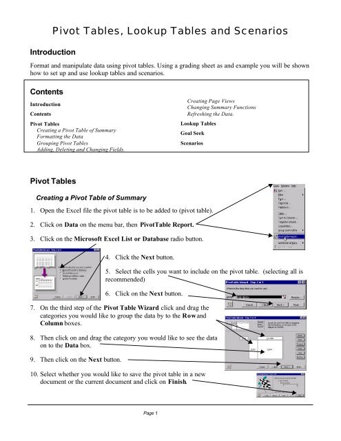
Pivot Tables, Lookup Tables and ScenariosIntroductionFormat and manipulate data using pivot tables. Using a grading sheet as and example you will be shownhow to set up and use lookup tables and scenarios.ContentsIntroductionContentsPivot TablesCreating a Pivot Table of SummaryFormatting the DataGrouping Pivot TablesAdding, Deleting and Changing Fields.Creating Page ViewsChanging Summary FunctionsRefreshing the Data.Lookup TablesGoal SeekScenariosPivot TablesCreating a Pivot Table of Summary1. Open the Excel file the pivot table is to be added to (pivot table).2. Click on Data on the menu bar, then PivotTable Report.3. Click on the Microsoft Excel List or Database radio button.4. Click the Next button.5. Select the cells you want to include on the pivot table. (selecting all isrecommended)6. Click on the Next button.7. On the third step of the Pivot Table Wizard click and drag thecategories you would like to group the data by to the Row andColumn boxes.8. Then click on and drag the category you would like to see the dataon to the Data box.9. Then click on the Next button.10. Select whether you would like to save the pivot table in a newdocument or the current document and click on Finish.Page 1

Pivot Tables, Lookup Tables and ScenariosFormatting the Data1. Highlight the cells formatting is desired for in the pivot table.2. Click on Format, Cells from the menu bar.3. On the format cells window select the formatting options desired on eachtab and click on OK when finished.Grouping Pivot Tables1. Click on the cell grouping is desired for. (This only works on dates andtimes)2. Click on Data on the menu bar and select Grouping and Outline, then clickon Group.3. Highlight the desired grouping categories and click on OK.Adding, Deleting and Changing Fields.1. Click on any cell in the pivot table.2. Click on the Pivot Table Wizard button on thePivotTable toolbox.3. Click on the field names and drag them to the desiredlocation. Click on Finish.Creating Page Views1. Click on a cell in the pivot table.2. Click on the Pivot Table Wizard button on the PivotTable toolbox.3. Drag the desired page-classifying field to the Page box and click onFinish.4. To view the different pages click on the down arrow on the top ofthe pivot table and click on the desired page.5. To make individual sheets for these pages click on the Show Pages button on the toolbar.Page 2

Pivot Tables, Lookup Tables and Scenarios6. Click on the desired page-classifier and click on OK.Changing Summary Functions1. Click on a cell in the pivot table.2. Click on the Pivot Table Wizard button on the toolbar.3. Double click on the field the summary function is to be changed in.4. Click on the desired summary function. Click on OK.5. Click on Finish.Refreshing the Data.1. Click Data on the menu bar.2. Click on Refresh Data.Lookup Tables1. Click on Insert in the menu bar and then click on Worksheet. (Thisnew table will be the lookup table that assigns a letter grade to eachstudent.)2. In Column A type in the grading scale. (The lowest numeric valuefor a grade should be entered. For example if a C is 70-79%, type 70. If roundingup is desired enter 69.5)3. In Column B type in the letter grade that corresponds to each percentagepoint.4. Click on the tab of a new worksheet, if there is not a blank one availableinsert one using the steps described in step 1.5. Set up your grade sheet, entering in the proper heading, formulas, and data toget a total percentage or point total for the class.7. Type =LOOKUP(8. Click on the cell that you would like to look up the letter grade of.Page 36. Click in the first empty cell under the columnLetter Grade.

Pivot Tables, Lookup Tables and Scenarios9. Type a comma. ,10. Then click on the Lookup Table’s worksheet tab on the bottom of the screen.11. Highlight the grading scale (column A) by clicking on the first value and dragging to the bottom.12. Type a comma. ,13. Highlight the letter grades these values get (column B) by the same fashion.14. Type a close parenthesis. )15. Make sure the formula’s are absolute (have a $ in font) if they are not insert a dollar sign in font oneach cell letter.Goal SeekUse Goal Seek to Determine an Optimal Grade Level.1. Click on the EDU 020 tab. Click to select cell G3.2. Select Tools on the menu bar, then Goal Seek.3. Type 75 in the To Value box.4. Click in the By Changing Cell box, and type E3 toindicate the 9/28 Test *3.5. Click OK6. The Goal Seek Status box appears with the answer to the question askedin the worksheet. Click OK to keep the new values in the worksheetor Cancel to keep the original values.ScenariosView how changing different figures in a situation can affect the outcome.1. Click on Tools, Scenarios.2. Click on the Add button.Page 4

Pivot Tables, Lookup Tables and Scenarios3. Type in the name or title of the Scenario (ie. Final Grade), and press the tab key.4. Holding the control key click on the cells that desired changes would like to be seen in. (B2, C2, D2,E2).5. Click on OK.6. Click on the Add button again.7. In the title box type Low Test. Press the tab key.8. In the test box change the score from 45 to 25. Click OK.9. Go through this process again making 2 or 3 different scenarios.10. When finished creating scenarios click on Summary button.11. Choose the cells you would like to summarize on and click on OK.Page 5