Applied Combinatorics - www.math.gatech.edu - Georgia Institute of ...

Applied CombinatoricsPreliminary EditionJanuary 6, 2013Mitchel T. KellerWilliam T. TrotterGeorgia Institute of Technology

Copyright c○ 2012 Mitchel T. Keller and William T. Trotter.This text is licensed under the CreativeCommons Attribution-NonCommercial-ShareAlike3.0 Unported (CC BY-NC-SA 3.0) license. For more details, please seehttp://creativecommons.org/licenses/by-nc-sa/3.0/This manuscript was typeset by the authors using the LATEX document processing system.

CONTENTSPrefacePrologueviixi1. An Introduction to Combinatorics 11.1. Introduction . . . . . . . . . . . . . . . . . . . . . . . . . . . . . . . . . . . . 11.2. Enumeration . . . . . . . . . . . . . . . . . . . . . . . . . . . . . . . . . . . . 21.3. Combinatorics and Graph Theory . . . . . . . . . . . . . . . . . . . . . . . 31.4. Combinatorics and Number Theory . . . . . . . . . . . . . . . . . . . . . . 61.5. Combinatorics and Geometry . . . . . . . . . . . . . . . . . . . . . . . . . . 91.6. Combinatorics and Optimization . . . . . . . . . . . . . . . . . . . . . . . . 101.7. Sudoku Puzzles . . . . . . . . . . . . . . . . . . . . . . . . . . . . . . . . . . 121.8. Discussion . . . . . . . . . . . . . . . . . . . . . . . . . . . . . . . . . . . . . 132. Strings, Sets, and Binomial Coecients 152.1. Strings: A First Look . . . . . . . . . . . . . . . . . . . . . . . . . . . . . . . 152.2. Permutations . . . . . . . . . . . . . . . . . . . . . . . . . . . . . . . . . . . 162.3. Combinations . . . . . . . . . . . . . . . . . . . . . . . . . . . . . . . . . . . 182.4. Combinatorial Proofs . . . . . . . . . . . . . . . . . . . . . . . . . . . . . . . 192.5. The Ubiquitous Nature of Binomial Coefficients . . . . . . . . . . . . . . . 212.6. The Binomial Theorem . . . . . . . . . . . . . . . . . . . . . . . . . . . . . . 252.7. Multinomial Coefficients . . . . . . . . . . . . . . . . . . . . . . . . . . . . . 262.8. Discussion . . . . . . . . . . . . . . . . . . . . . . . . . . . . . . . . . . . . . 272.9. Exercises . . . . . . . . . . . . . . . . . . . . . . . . . . . . . . . . . . . . . . 283. Induction 353.1. Introduction . . . . . . . . . . . . . . . . . . . . . . . . . . . . . . . . . . . . 353.2. The Positive Integers are Well Ordered . . . . . . . . . . . . . . . . . . . . 36i

Contents3.3. The Meaning of Statements . . . . . . . . . . . . . . . . . . . . . . . . . . . 363.4. Binomial Coefficients Revisited . . . . . . . . . . . . . . . . . . . . . . . . . 383.5. Solving Combinatorial Problems Recursively . . . . . . . . . . . . . . . . . 393.6. Mathematical Induction . . . . . . . . . . . . . . . . . . . . . . . . . . . . . 433.7. Inductive Definitions . . . . . . . . . . . . . . . . . . . . . . . . . . . . . . . 443.8. Proofs by Induction . . . . . . . . . . . . . . . . . . . . . . . . . . . . . . . . 453.9. Strong Induction . . . . . . . . . . . . . . . . . . . . . . . . . . . . . . . . . 473.10. Discussion . . . . . . . . . . . . . . . . . . . . . . . . . . . . . . . . . . . . . 483.11. Exercises . . . . . . . . . . . . . . . . . . . . . . . . . . . . . . . . . . . . . . 494. Combinatorial Basics 514.1. The Pigeon Hole Principle . . . . . . . . . . . . . . . . . . . . . . . . . . . . 514.2. An Introduction to Complexity Theory . . . . . . . . . . . . . . . . . . . . 524.3. The Big “Oh” and Little “Oh” Notations . . . . . . . . . . . . . . . . . . . 554.4. Exact Versus Approximate . . . . . . . . . . . . . . . . . . . . . . . . . . . . 564.5. Discussion . . . . . . . . . . . . . . . . . . . . . . . . . . . . . . . . . . . . . 584.6. Exercises . . . . . . . . . . . . . . . . . . . . . . . . . . . . . . . . . . . . . . 585. Graph Theory 615.1. Basic Notation and Terminology for Graphs . . . . . . . . . . . . . . . . . 615.2. Multigraphs: Loops and Multiple Edges . . . . . . . . . . . . . . . . . . . . 665.3. Eulerian and Hamiltonian Graphs . . . . . . . . . . . . . . . . . . . . . . . 675.4. Graph Coloring . . . . . . . . . . . . . . . . . . . . . . . . . . . . . . . . . . 715.5. Planar Graphs . . . . . . . . . . . . . . . . . . . . . . . . . . . . . . . . . . . 775.6. Counting Labeled Trees . . . . . . . . . . . . . . . . . . . . . . . . . . . . . 855.7. A Digression into Complexity Theory . . . . . . . . . . . . . . . . . . . . . 895.8. Discussion . . . . . . . . . . . . . . . . . . . . . . . . . . . . . . . . . . . . . 905.9. Exercises . . . . . . . . . . . . . . . . . . . . . . . . . . . . . . . . . . . . . . 906. Partially Ordered Sets 1016.1. Basic Notation and Terminology . . . . . . . . . . . . . . . . . . . . . . . . 1026.2. Additional Concepts for Posets . . . . . . . . . . . . . . . . . . . . . . . . . 1066.3. Dilworth’s Chain Covering Theorem and its Dual . . . . . . . . . . . . . . 1096.4. Linear Extensions of Partially Ordered Sets . . . . . . . . . . . . . . . . . . 1126.5. The Subset Lattice . . . . . . . . . . . . . . . . . . . . . . . . . . . . . . . . . 1136.6. Interval Orders . . . . . . . . . . . . . . . . . . . . . . . . . . . . . . . . . . 1156.7. Finding a Representation of an Interval Order . . . . . . . . . . . . . . . . 1166.8. Dilworth’s Theorem for Interval Orders . . . . . . . . . . . . . . . . . . . . 1186.9. Discussion . . . . . . . . . . . . . . . . . . . . . . . . . . . . . . . . . . . . . 1206.10. Exercises . . . . . . . . . . . . . . . . . . . . . . . . . . . . . . . . . . . . . . 120iiCopyright c○2010–2012

Contents7. Inclusion-Exclusion 1277.1. Introduction . . . . . . . . . . . . . . . . . . . . . . . . . . . . . . . . . . . . 1277.2. The Inclusion-Exclusion Formula . . . . . . . . . . . . . . . . . . . . . . . . 1307.3. Enumerating Surjections . . . . . . . . . . . . . . . . . . . . . . . . . . . . . 1317.4. Derangements . . . . . . . . . . . . . . . . . . . . . . . . . . . . . . . . . . . 1337.5. The Euler φ Function . . . . . . . . . . . . . . . . . . . . . . . . . . . . . . . 1357.6. Discussion . . . . . . . . . . . . . . . . . . . . . . . . . . . . . . . . . . . . . 1377.7. Exercises . . . . . . . . . . . . . . . . . . . . . . . . . . . . . . . . . . . . . . 1378. Generating Functions 1438.1. Basic Notation and Terminology . . . . . . . . . . . . . . . . . . . . . . . . 1438.2. Another look at distributing apples or folders . . . . . . . . . . . . . . . . 1458.3. Newton’s Binomial Theorem . . . . . . . . . . . . . . . . . . . . . . . . . . 1488.4. An Application of the Binomial Theorem . . . . . . . . . . . . . . . . . . . 1498.5. Partitions of an Integer . . . . . . . . . . . . . . . . . . . . . . . . . . . . . . 1518.6. Exponential generating functions . . . . . . . . . . . . . . . . . . . . . . . . 1528.7. Discussion . . . . . . . . . . . . . . . . . . . . . . . . . . . . . . . . . . . . . 1558.8. Exercises . . . . . . . . . . . . . . . . . . . . . . . . . . . . . . . . . . . . . . 1559. Recurrence Equations 1639.1. Introduction . . . . . . . . . . . . . . . . . . . . . . . . . . . . . . . . . . . . 1639.2. Linear Recurrence Equations . . . . . . . . . . . . . . . . . . . . . . . . . . 1679.3. Advancement Operators . . . . . . . . . . . . . . . . . . . . . . . . . . . . . 1689.4. Solving advancement operator equations . . . . . . . . . . . . . . . . . . . 1709.5. Formalizing our approach to recurrence equations . . . . . . . . . . . . . . 1789.6. Using generating functions to solve recurrences . . . . . . . . . . . . . . . 1829.7. Solving a nonlinear recurrence . . . . . . . . . . . . . . . . . . . . . . . . . 1849.8. Discussion . . . . . . . . . . . . . . . . . . . . . . . . . . . . . . . . . . . . . 1879.9. Exercises . . . . . . . . . . . . . . . . . . . . . . . . . . . . . . . . . . . . . . 18710.Probability 19110.1. An Introduction to Probability . . . . . . . . . . . . . . . . . . . . . . . . . 19210.2. Conditional Probability and Independent Events . . . . . . . . . . . . . . . 19410.3. Bernoulli Trials . . . . . . . . . . . . . . . . . . . . . . . . . . . . . . . . . . 19510.4. Discrete Random Variables . . . . . . . . . . . . . . . . . . . . . . . . . . . 19610.5. Central Tendency . . . . . . . . . . . . . . . . . . . . . . . . . . . . . . . . . 19810.6. Probability Spaces with Infinitely Many Outcomes . . . . . . . . . . . . . 20210.7. Discussion . . . . . . . . . . . . . . . . . . . . . . . . . . . . . . . . . . . . . 20310.8. Exercises . . . . . . . . . . . . . . . . . . . . . . . . . . . . . . . . . . . . . . 20411.Applying Probability to Combinatorics 20711.1. Small Ramsey Numbers . . . . . . . . . . . . . . . . . . . . . . . . . . . . . 209Mitchel T. Keller and William T. Trotteriii

Contents16.4. Miscellaneous Gems . . . . . . . . . . . . . . . . . . . . . . . . . . . . . . . 29416.5. Zero–One Matrices . . . . . . . . . . . . . . . . . . . . . . . . . . . . . . . . 29516.6. Arithmetic Combinatorics . . . . . . . . . . . . . . . . . . . . . . . . . . . . 29716.7. The Lovasz Local Lemma . . . . . . . . . . . . . . . . . . . . . . . . . . . . 29716.8. Applying the Local Lemma . . . . . . . . . . . . . . . . . . . . . . . . . . . 300Epilogue 303A. Appendix: Background Material for Combinatorics 305A.1. Introduction . . . . . . . . . . . . . . . . . . . . . . . . . . . . . . . . . . . . 305A.2. Intersections and Unions . . . . . . . . . . . . . . . . . . . . . . . . . . . . . 307A.3. Cartesian Products . . . . . . . . . . . . . . . . . . . . . . . . . . . . . . . . 309A.4. Binary Relations and Functions . . . . . . . . . . . . . . . . . . . . . . . . . 309A.5. Finite Sets . . . . . . . . . . . . . . . . . . . . . . . . . . . . . . . . . . . . . 311A.6. Notation from Set Theory and Logic . . . . . . . . . . . . . . . . . . . . . . 312A.7. Formal Development of Number Systems . . . . . . . . . . . . . . . . . . . 313A.8. Multiplication as a Binary Operation . . . . . . . . . . . . . . . . . . . . . . 316A.9. Exponentiation . . . . . . . . . . . . . . . . . . . . . . . . . . . . . . . . . . 318A.10.Partial Orders and Total Orders . . . . . . . . . . . . . . . . . . . . . . . . . 318A.11.A Total Order on Natural Numbers . . . . . . . . . . . . . . . . . . . . . . 319A.12.Notation for Natural Numbers . . . . . . . . . . . . . . . . . . . . . . . . . 320A.13.Equivalence Relations . . . . . . . . . . . . . . . . . . . . . . . . . . . . . . 322A.14.The Integers as Equivalence Classes of Ordered Pairs . . . . . . . . . . . . 323A.15.Properties of the Integers . . . . . . . . . . . . . . . . . . . . . . . . . . . . 323A.16.Obtaining the Rationals from the Integers . . . . . . . . . . . . . . . . . . . 325A.17.Obtaining the Reals from the Rationals . . . . . . . . . . . . . . . . . . . . 327A.18.Obtaining the Complex Numbers from the Reals . . . . . . . . . . . . . . . 328A.19.The Zermelo-Fraenkel Axioms of Set Theory . . . . . . . . . . . . . . . . . 330Mitchel T. Keller and William T. Trotterv

PREFACEAt Georgia Tech, MATH 3012: Applied Combinatorics, is a junior-level course targetedprimarily at students pursuing the B.S. in Computer Science. The purpose ofthe course is to give students a broad exposure to combinatorial mathematics, usingapplications to emphasize fundamental concepts and techniques. Applied Combinatoricsis also required of students seeking the B.S. in Applied Mathematics or the B.Sin Discrete Mathematics, and it is one of two discrete mathematics courses that computerengineering students may select to fulfill a breadth requirement. The course willalso often contain a selection of other engineering and science majors who are interestedin learning more mathematics. As a consequence, in a typical semester, some250 Georgia Tech students are enrolled in Applied Combinatorics. Students enrolledin Applied Combinatorics at Georgia Tech have already completed the three semestercalculus sequence—with many students bypassing one or more of the these courseson the basis of advanced placement scores. Also, the students will know some linearalgebra and can at least have a reasonable discussion about vector spaces, bases anddimension.Our approach to the course is to show students the beauty of combinatorics andhow combinatorial problems naturally arise in many settings, particularly in computerscience. While proofs are periodically presented in class, the course is not intended toteach students how to write proofs; there are other required courses in our curriculumthat meet this need. Students may occasionally be asked to prove small facts, but thesearguments are closer to the kind we expect from students in second or third semestercalculus as contrasted with proofs we expect from a mathematics major in an upperdivisioncourse. Regardless, we cut very few corners, and our text can readily be usedby instructors who elect to be even more rigorous in their approach.This book arose from our feeling that a text that met our approach to Applied Combinatoricswas not available. Because of the diverse set of instructors assigned to thecourse, the standard text was one that covered every topic imaginable (and then some),but provided little depth. We’ve taken a different approach, attacking the central subjectsof the course description to provide exposure, but taking the time to go intogreater depth in select areas to give the students a better feel for how combinatoricsworks. We have also included some results and topics that are not found in other textsat this level but help reveal the nature of combinatorics to students. We want studentsvii

Prefaceto understand that combinatorics is a subject that you must feel “in the gut”, and wehope that our presentation achieves this goal. The emphasis throughout remains onapplications, including algorithms. We do not get deeply into the details of what itmeans for an algorithm to be “efficient”, but we do include an informal discussion ofthe basic principles of complexity, intended to prepare students in computer science,engineering and applied mathematics for subsequent coursework.The materials included in this book have evolved over time. Early versions of a fewchapters date from 2004, but the pace quickened in 2006 when the authors team taughta large section of Applied Combinatorics. In the last five years, existing chapters havebeen updated and expanded, while new chapters have been added. As matters nowstand, our book includes more material than we can cover in a single semester. We feelthat the topics of Chapters 1 through 9 plus Chapters 12, 13 and 14 are the core of aone semester course in Applied Combinatorics. Additional topics can then be selectedfrom the remaining chapters based on the interests of the instructor and students.We are grateful to our colleagues Alan Diaz, Thang Le, Noah Strebi, Prasad Tetaliand Carl Yerger, who have taught Applied Combinatorics from preliminary versionsand have given valuable feedback. As this text is freely available on the internet, wewelcome comments, criticisms, suggestions and corrections from anyone who takes alook at our work.About the AuthorsWilliam T. Trotter is a Professor in the School of Mathematics at Georgia Tech. He wasfirst exposed to combinatorial mathematics through the 1971 Bowdoin CombinatoricsConference which featured an array of superstars of that era, including Gian CarloRota, Paul Erdős, Marshall Hall, Herb Ryzer, Herb Wilf, William Tutte, Ron Graham,Daniel Kleitman and Ray Fulkerson. Since that time, he has published more than 120research papers on graph theory, discrete geometry, ramsey theory and extremal combinatorics.Perhaps his best known work is in the area of combinatorics and partiallyordered sets, and his 1992 research monograph on this topic has been very influential(he takes some pride in the fact that this monograph is still in print and copies arebeing sold in 2012). He has more than 70 co-authors, but considers his extensive jointwork with Graham Brightwell, Stefan Felsner, Peter Fishburn, Hal Kierstead and EndreSzemerèdi as representing his best work. His career includes invited presentationsat more than 50 international conferences and more than 30 meetings of professionalsocieties. He was the founding editor of the SIAM Journal on Discrete Mathematics andhas served on the Editorial Board of Order since the journal was launched in 1984, andhis service includes an eight year stint as Editor-in-Chief. Currently, he serves on theeditorial boards of three other journals in combinatorial mathematics.viiiCopyright c○2010–2012

Still he has his quirks. First, he insists on being called “Tom”, as Thomas is his middlename, while continuing to sign as William T. Trotter. Second, he has invested timeand energy serving five terms as department/school chair, one at Georgia Tech, twoat Arizona State University and two at the University of South Carolina. In addition,he has served as a Vice Provost and as an Assistant Dean. Third, he is fascinated bycomputer operating systems and is always installing new ones. In one particular week,he put eleven different flavors of Linux on the same machine, interspersed with fourcomplete installs of Windows 7. Incidentally, the entire process started and ended withWindows 7. Fourth, he likes to hit golf balls, not play golf, just hit balls. Without thesediversions, he might even have had enough time to settle the Riemann hypothesis.He has had eleven Ph.D. students, one of which is now his co-author on this text.Mitchel T. Keller is a super-achiever (this description is written by WTT) extraordinairefrom North Dakota. As a graduate student at Georgia Tech, he won a lengthy list ofhonors and awards, including a Vigre Graduate Fellowship, an IMPACT Scholarship,a John R. Festa Fellowship and the 2009 Price Research Award. Mitch is a naturalleader and was elected President (and Vice President) of the Georgia Tech GraduateStudent Governance Association, roles in which he served with distinction. Indeed,after completing his terms, his student colleagues voted to establish a continuing awardfor distinguished leadership, to be named the Mitchel T. Keller award, with Mitch asthe first recipient. Very few graduate students win awards in the first place, but Mitchis the only one I know who has an award named after them.Mitch is also a gifted teacher of mathematics, receiving the prestigious Georgia Tech2008 Outstanding Teacher Award, a campus-wide competition. He is quick to experimentwith the latest approaches to teaching mathematics, adopting what works forhim while refining and polishing things along the way. He really understands the literaturebehind active learning and the principles of engaging students in the learningprocess. Mitch has even taught his more senior (some say ancient) co-author a thing ortwo and got him to try personal response systems in a large calculus section this fall.Mitch is off to a fast start in his own research career, and is already an expert in thesubject of linear discrepancy. Mitch has also made substantive contributions to a topicknown as Stanley depth, which is right at the boundary of combinatorial mathematicsand algebraic combinatorics.Mitchel T. Keller and William T. Trotterix

PrefaceAfter finishing his Ph.D., Mitch received another signal honor, a Marshall SherfieldPostdoctoral Fellowship and has spent the last two years at the London School ofEconomics. A year from now, Mitch will be at a new place and a few years down theroad, he’ll probably be president of something.On the personal side, Mitch is the keeper of the Mathematical Genealogy Project,and he is a great cook. His desserts are to die for.Mitch Keller, keller@rellek.netTom Trotter, trotter@math.gatech.eduAtlanta, GeorgiaxCopyright c○2010–2012

PROLOGUEA unique feature of this book is a recurring cast of characters: Alice, Bob, Carlos, Dave,Xing, Yolanda and Zori. They are undergraduate students at Georgia Tech, they’retaking an 8:05am section of Math 3012: Applied Combinatorics, and they frequentlygo for coffee at the Clough Undergraduate Learning Center immendiately after theclass is over. They’ve become friends of sorts and you may find their conversationsabout Applied Combinatorics of interest, as they will may reveal subtleties behindtopics currently being studied, reinforce connections with previously studied materialor set the table for topics which will come later. Sometimes, these conversations willset aside in a clearly marked Dicussion section, but they will also be sprinkled as briefremarks throughout the text.In time, you will get to know these characters and will sense that, for example, whenDave comments on a topic, it will represent a perspective that Zori is unlikely to share.Some comments are right on target while others are “out in left field.” Some mayeven be humorous, at least we hope this is the case. Regardless, our goal is not toentertain—although that is not all that bad a side benefit. Instead, we intend that ourinformal approach adds to the instructional value of our text.Now it is time to meet our characters.Alice is a computer engineering major from Philadelphia. She is ambitious, smart andintense. Alice is quick to come to conclusions, most of which are right. On occasion,Alice is not kind to Bob.Bob is a management major from Omaha. He is a hard working and conscientious.Bob doesn’t always keep pace with his friends, but anything he understands, he owns,and in the end, he gets almost everything. On the other hand, Bob has never quiteunderstood why Alice is short with him at times.Carlos is a really, really smart physics major from San Antonio. He has three olderbrothers and two sisters, one older, one younger. His high school background wasn’tall that great, but Carlos is clearly a special student at Georgia Tech. He absorbs newconcepts at lightning speed and sees through to the heart of almost every topic. Hethinks carefully before he says something and is admirably polite.Dave is a discrete math major from Los Angeles. Dave is a flake. He’s plenty smartxi

Prologueenough but not all that diligent. Still, he has unique insights into things and from timeto time says something worth hearing—not always but sometimes. His friends say thatDave suffers from occasional brain–mouth disconnects.Xing is a computer science major from New York. Xing’s parents immigrated fromBeijing, and he was strongly supported and encouraged in his high school studies.Xing is detail oriented and not afraid to work hard.Yolanda is a double major (computer science and chemistry) from Cumming, a smalltown just north of Atlanta. Yolanda is the first in her extended family to go to a collegeor university. She is smart and absorbs knowledge like a sponge. It’s all new to herand her horizons are raised day by day.Zori is an applied math major from Detroit. She is bottom-line focused, has little timefor puzzles and always wants to see applications to justify why something is includedin the course. Zori is determined, driven and impatient at times.xiiCopyright c○2010–2012

CHAPTERONEAN INTRODUCTION TO COMBINATORICSAs we hope you will sense right from the beginning, we believe that combinatorialmathematics is one of the most fascinating and captivating subjects on the planet.Combinatorics is very concrete and has a wide range of applications, but it also hasan intellectually appealing theoretical side. Our goal is to give you a taste of both. Inorder to begin, we want to develop, through a series of examples, a feeling for whattypes of problems combinatorics addresses.1.1. IntroductionThere are three principal themes to our course:Discrete Structures Graphs, digraphs, networks, designs, posets, strings, patterns,distributions, coverings, and partitions.Enumeration Permutations, combinations, inclusion/exclusion, generating functions,recurrence relations, and Pólya counting.Algorithms and Optimization Sorting, spanning trees, shortest paths, eulerian circuits,hamiltonian cycles, graph coloring, planarity testing, network flows, bipartitematchings, and chain partitions.To illustrate the accessible, concrete nature of combinatorics and to motivate topicsthat we will study, this preliminary chapter provides a first look at combinatorialproblems, choosing examples from enumeration, graph theory, number theory, andoptimization. The discussion is very informal—but this should serve to explain whywe have to be more precise at later stages. We ask lots of questions, but at this stage,you’ll only be able to answer a few. Later, you’ll be able to answer many more . . . but1

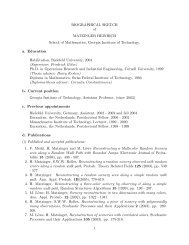
Chapter 1. An Introduction to Combinatoricsas promised earlier, most likely you’ll never be able to answer them all. And if we’rewrong in making that statement, then you’re certain to become very famous. Also,you’ll get an A++ in the course and maybe even a Ph.D. too.1.2. EnumerationMany basic problems in combinatorics involve counting the number of distributionsof objects into cells—where we may or may not be able to distinguish between theobjects and the same for the cells. Also, the cells may be arranged in patterns. Hereare concrete examples.Amanda has three children: Dawn, Keesha and Seth.1. Amanda has ten one dollar bills and decides to give the full amount to her children.How many ways can she do this? For example, one way she might distributethe funds is to give Dawn and Keesha four dollars each with Seth receivingthe balance—two dollars. Another way is to give the entire amount to Keesha,an option that probably won’t make Dawn and Seth very happy. Note that hiddenwithin this question is the assumption that Amanda does not distinguish theindividual dollar bills, say by carefully examining their serial numbers. Instead,we intennd that she need only decide the amount each of the three children is toreceive.2. The amounts of money distributed to the three children form a sequence whichif written in non-increasing order has the form: a 1 , a 2 , a 3 with a 1 ≥ a 2 ≥ a 3 anda 1 + a 2 + a 3 = 10. How many such sequences are there?3. Suppose Amanda decides to give each child at least one dollar. How does thischange the answers to the first two questions?4. Now suppose that Amanda has ten books, in fact the top 10 books from the NewYork Times best-seller list, and decides to give them to her children. How manyways can she do this? Again, we note that there is a hidden assumption—the tenbooks are all different.5. Suppose the ten books are labeled B 1 , B 2 , . . . , B 10 . The sets of books given to thethree children are pairwise disjoint and their union is {B 1 , B 2 , . . . , B 10 }. Howmany different sets of the form {S 1 , S 2 , S 3 } where S 1 , S 2 and S 3 are pairwisedisjoint and S 1 ∪ S 2 ∪ S 3 = {B 1 , B 2 , . . . , B 10 }?6. Suppose Amanda decides to give each child at least one book. How does thischange the answers to the preceding two questions?2 Copyright c○2010–2012

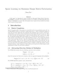
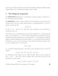
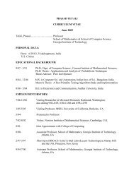
1.3. Combinatorics and Graph TheoryFigure 1.1.: Necklaces made with three colors7. How would we possibly answer these kinds of questions if ten was really tenthousand (OK, we’re not talking about children any more!) and three was threethousand? Could you write the answer on a single page in a book?A circular necklace with a total of six beads will be assembled using beads of threedifferent colors. In Figure 1.1, we show four such necklaces—however, note that thefirst three are actually the same necklace. Each has three red beads, two blues and onegreen. On the other hand, the fourth necklace has the same number of beads of eachcolor but it is a different necklace.1. How many different necklaces of six beads can be formed using three reds, twoblues and one green?2. How many different necklaces of six beads can be formed using red, blue andgreen beads (not all colors have to be used)?3. How many different necklaces of six beads can be formed using red, blue andgreen beads if all three colors have to be used?4. How would we possibly answer these questions for necklaces of six thousandbeads made with beads from three thousand different colors? What special softwarewould be required to find the exact answer and how long would the computationtake?1.3. Combinatorics and Graph TheoryA graph G consists of a vertex set V and a collection E of 2-element subsets of V. Elementsof E are called edges. In our course, we will (almost always) use the conventionthat V = {1, 2, 3, . . . , n} for some positive integer n. With this convention, graphs canbe described precisely with a text file:1. The first line of the file contains a single integer n, the number of vertices in thegraph.Mitchel T. Keller and William T. Trotter 3

Chapter 1. An Introduction to Combinatoricsgraph1.txt96 21 51 76 89 14 35 71 35 97 9431256798Figure 1.2.: A graph defined by data2. Each of the remaining lines of the file contains a pair of distinct integers andspecifies an edge of the graph.We illustrate this convention in Figure 1.2 with a text file and the diagram for thegraph G it defines.Much of the notation and terminology for graphs is quite natural. See if you canmake sense out of the following statements which apply to the graph G defined above:1. G has 9 vertices and 10 edges.2. {2, 6} is an edge.3. Vertices 5 and 9 are adjacent.4. {5, 4} is not an edge.5. Vertices 3 and 7 are not adjacent.6. P = (4, 3, 1, 7, 9, 5) is a path of length 5 from vertex 4 to vertex 5.7. C = (5, 9, 7, 1) is cycle of length 4.8. G is disconnected and has two components. One of the components has vertexset {2, 6, 8}.9. {1, 5, 7} is a triangle.10. {1, 7, 5, 9} is a clique of size 4.11. {4, 2, 8, 5} is an independent set of size 4.4 Copyright c○2010–2012

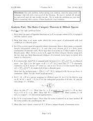
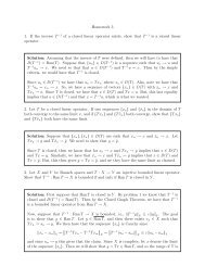
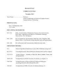
1.3. Combinatorics and Graph Theory741819824311195101220151422116171323226Figure 1.3.: A connected graphEquipped only with this little bit of background material, we are already able to posea number of interesting and challenging problems.Example 1.1. Consider the graph G shown in Figure 1.3.1. What is the largest k for which G has a path of length k?2. What is the largest k for which G has a cycle of length k?3. What is the largest k for which G has a clique of size k?4. What is the largest k for which G has an independent set of size k?5. What is the shortest path from vertex 7 to vertex 6?Suppose we gave the class a text data file for a graph on 1500 vertices and askedwhether the graph contains a cycle of length at least 500. Raoul says yes and Carlasays no. How do we decide who is right?Suppose instead we asked whether the graph has a clique of size 500. Helene saysthat she doesn’t think so, but isn’t certain. Is it reasonable that her classmates insistthat she make up her mind, one way or the other? Is determining whether this graphhas a clique of size 500 harder, easier or more or less the same as determining whetherit has a cycle of size 500.We will frequently study problems in which graphs arise in a very natural manner.Here’s an example.Example 1.2. In Figure 1.4, we show the location of some radio stations in the plane,together with a scale indicating a distance of 200 miles. Radio stations that are closerthan 200 miles apart must broadcast on different frequencies to avoid interference.Mitchel T. Keller and William T. Trotter 5

Chapter 1. An Introduction to Combinatorics651256444 65 33 64112651534200 milesFigure 1.4.: Radio StationsWe’ve shown that 6 different frequencies are enough. Can you do better?Can you find 4 stations each of which is within 200 miles of the other 3? Can youfind 8 stations each of is more than 200 miles away from the other 7? Is there a naturalway to define a graph associated with this problem?Example 1.3. How big must an applied combinatorics class be so that there are either(a) six students with each pair having taken at least one other class together, or (b) sixstudents with each pair together in a class for the first time. Is this really a hardproblem or can we figure it out in just a few minutes, scribbling on a napkin?1.4. Combinatorics and Number TheoryBroadly, number theory concerns itself with the properties of the positive integers.G.H. Hardy was a brilliant British mathematician who lived through both World Warsand conducted a large deal of number-theoretic research. He was also a pacifist whowas happy that, from his perspective, his research was not “useful”. He wrote in his1940 essay A Mathematician’s Apology “[n]o one has yet discovered any warlike purposeto be served by the theory of numbers or relativity, and it seems very unlikely thatanyone will do so for many years.” 1 Little did he know, the purest mathematical ideasof number theory would soon become indispensable for the cryptographic techniquesthat kept communications secure. Our subject here is not number theory, but we willsee a few times where combinatorial techniques are of use in number theory.1 G.H. Hardy, A Mathematician’s Apology, Cambridge University Press, p. 140. (1993 printing)6 Copyright c○2010–2012

1.4. Combinatorics and Number TheoryExample 1.4. Form a sequence of positive integers using the following rules. Start witha positive integer n > 1. If n is odd, then the next number is 3n + 1. If n is even, thenthe next number is n/2. Halt if you ever reach 1. For example, if we start with 28, thesequence is28, 14, 7, 22, 11, 34, 17, 52, 26, 13, 40, 20, 10, 5, 16, 8, 4, 2, 1.Now suppose you start with 19. Then the first few terms are19, 58, 29, 88, 44, 22.But now we note that the integer 22 appears in the first sequence, so the two sequenceswill agree from this point on. Sequences formed by this rule are called Collatz sequences.Pick a number somewhere between 100 and 200 and write down the sequence youget. Regardless of your choice, you will eventually halt with a 1. However, is theresome positive integer n (possibly quite large) so that if you start from n, you will neverreach 1?Example 1.5. Students in middle school are taught to add fractions by finding leastcommon multiples. For example, the least common multiple of 15 and 12 is 60, so:215 + 712 = 860 + 3560 = 4360 .How hard is it to find the least common multiple of two integers? It’s really easyif you can factor them into primes. For example, consider the problem of finding theleast common multiple of 351785000 and 316752027900 if you just happen to know thatThen the least common multiple is351785000 =2 3 × 5 4 × 7 × 19 × 23 2 and316752027900 =2 2 × 3 × 5 2 × 7 3 × 11 × 23 4 .300914426505000 =2 3 × 3 × 5 4 × 7 3 × 11 × 19 × 23 4 .So to find the least common multiple of two numbers, we just have to factor them intoprimes. That doesn’t sound too hard. For starters, can you factor 1961? OK, how about1348433? Now for a real challenge. Suppose you are told that the integerc = 5220070641387698449504000148751379227274095462521is the product of two primes a and b. Can you find them?What if factoring is hard? Can you find the least common multiple of two relativelylarge integers, say each with about 500 digits, by another method? How should middleschool students be taught to add fractions?Mitchel T. Keller and William T. Trotter 7

Chapter 1. An Introduction to CombinatoricsAs an aside, we note that most calculators can’t add or multiply two 20 digits numbers,much less two numbers with more than 500 digits. But it is relatively straightforwardto write a computer program that will do the job for us. Also, there are somepowerful mathematical software tools available. Two very well known examples areMaple R○ and Mathematica R○ . For example, if you open up a Maple workspace and enterthe command:ifactor(300914426505000);then about as fast as you hit the carriage return, you will get the prime factorizationshown above.Now here’s how we made up the challenge problem. First, we found a site on theweb that lists large primes and found these two values:a =45095080578985454453andb =115756986668303657898962467957.We then used Maple to multiply them together using the following command:45095080578985454453 ∗ 115756986668303657898962467957;Almost instantly, Maple reported the value for c given above.Out of curiosity, we then asked Maple to factor c. It took almost 12 minutes on apowerful desktop computer.Questions arising in number theory can also have an enumerative flair, as the followingexample shows.Example 1.6. In Table 1.1, we show the integer partitions of 8. There are 22 partitions8 distinct parts 7+1 distinct parts, odd parts 6+2 distinct parts6+1+1 5+3 distinct parts, odd parts 5+2+1 distinct parts5+1+1+1 odd parts 4+4 4+3+1 distinct parts4+2+2 4+2+1+1 4+1+1+1+13+3+2 3+3+1+1 odd parts 3+2+2+13+2+1+1+1 3+1+1+1+1+1 odd parts 2+2+2+22+2+2+1+1 2+2+1+1+1+1 2+1+1+1+1+1+11+1+1+1+1+1+1+1 odd partsTable 1.1.: The partitions of 8, noting those into distinct parts and those intoodd parts.altogether, and as noted, exactly 6 of them are partitions of 8 into odd parts. Also,exactly 6 of them are partitions of 8 into distinct parts.8 Copyright c○2010–2012

1.5. Combinatorics and GeometryWhat would be your reaction if we asked you to find the number of integer partitionsof 25892? Do you think that the number of partitions of 25892 into odd parts equalsthe number of partitions of 25892 into distinct parts? Is there a way to answer thisquestion without actually calculating the number of partitions of each type?1.5. Combinatorics and GeometryThere are many problems in geometry that are innately combinatorial or for whichcombinatorial techniques shed light on the problem.Example 1.7. In Figure 1.5, we show a family of 4 lines in the plane. Each pair oflines intersects and no point in the plane belongs to more than two lines. These linesdetermine 11 regions.3152678491011Figure 1.5.: Lines and regionsUnder these same restrictions, how many regions would a family of 8947 lines determine?Can different arrangements of lines determine different numbers of regions?Example 1.8. Mandy says she has found a set of 882 points in the plane that determineexactly 752 lines. Tobias disputes her claim. Who is right?Example 1.9. There are many different ways to draw a graph in the plane. Some drawingsmay have crossing edges while others don’t. But sometimes, crossing edges mustappear in any drawing. Consider the graph G shown in Figure 1.6. Can you redraw Gwithout crossing edges?Suppose Sam and Deborah were given a homework problem asking whether a particulargraph on 2843952 vertices and 9748032 edges could be drawn without edgeMitchel T. Keller and William T. Trotter 9

Chapter 1. An Introduction to Combinatorics5410312697 8Figure 1.6.: A graph with crossing edgescrossings. Deborah just looked at the number of vertices and the number of edgesand said that the answer is “no.” Sam questions how she can be so certain—withoutlooking more closely at the structure of the graph. Is there a way for Deborah to justifyher definitive response?1.6. Combinatorics and OptimizationYou likely have already been introduced to optimization problems, as calculus studentsaround the world are familiar with the plight of farmers trying to fence thelargest area of land given a certain amount of fence or people needing to cross riversdownstream from their current location who must decide where they should crossbased on the speed at which they can run and swim. However, these problems areinherently continuous. In theory, you can cross the river at any point you want, evenif it were irrational. (OK, so not exactly irrational, but a good decimal approximation.)In this course, we will examine a few optimization problems that are not continuous,as only integer values for the variables will make sense. It turns out that many of theseproblems are very hard to solve in general.Example 1.10. In Figure 1.7, we use letters for the labels on the vertices to help distinguishvisually from the integer weights on the edges.Suppose the vertices are cities, the edges are highways and the weights on the edgesrepresent distance.Q 1 : What is the shortest path from vertex E to vertex B?Suppose Ariel is a salesperson whose home base is city A.Q 2 : In what order should Ariel visit the other cities so that she goes through eachof them at least once and returns home at the end—while keeping the total distance10 Copyright c○2010–2012

1.6. Combinatorics and OptimizationE1312 28F 727 10J11K189 8A193216C3GH5174142BDFigure 1.7.: A labeled graph with weighted edgestraveled to a minimum? Can Ariel accomplish such a tour visiting each city exactlyonce?Sanjay is a highway inspection engineer and must traverse every highway eachmonth. Sanjay’s homebase is City E.Q 3 : In what order should Sanjay traverse the highways to minimize the total distancetraveled? Can Sanjay make such a tour traveling along each highway exactly once?Example 1.11. Now suppose that the vertices are locations of branch banks in Atlantaand that the weights on an edge represents the cost, in millions of dollars, of buildinga high capacity data link between the branch banks at it two end points. In this model,if there is no edge between two branch banks, it means that the cost of building a datalink between this particular pair is prohibitively high (here we might be tempted to saythe cost is infinite, but the authors don’t admit to knowing the meaning of this word).Our challenge is to decide which data links should be constructed to form a networkin which any branch bank can communicate with any other branch. We assume thatdata can flow in either direction on a link, should it be built, and that data can berelayed through any number of data links. So to allow full communication, we shouldconstruct a spanning tree in this network. In Figure 1.8, we show a graph G on the leftand one of its many spanning trees on the right.The weight of the spanning tree is the sum of the weights on the edges. In our model,this represents the costs, again in millions of dollars, of building the data links associatedwith the edges in the spanning tree. For the spanning tree shown in Figure 1.8,this total is12 + 25 + 19 + 18 + 23 + 19 = 116.Mitchel T. Keller and William T. Trotter 11

Chapter 1. An Introduction to CombinatoricsE12251328GB1918CBE25G1912 18CF141623F232719A19ADDFigure 1.8.: A weighted graph and spanning treeOf all spanning trees, the bank would naturally like to find one having minimumweight.How many spanning trees does this graph have? For a large graph, say one with2875 vertices, does it make sense to find all spanning trees and simply take the onewith minimum cost? In particular, for a positive integer n, how many trees have vertexset {1, 2, 3, . . . , n}?1.7. Sudoku PuzzlesHere’s an example which has more substance than you might think at first glance. Itinvolves Sudoku puzzles, which have become immensely popular in recent years.Example 1.12. A Sudoku puzzle is a 9 × 9 array of cells that when completed have theintegers 1, 2, . . . , 9 appearing exactly once in each row and each column. Also (and thisis what makes the puzzles so fascinating), the numbers 1, 2, 3, . . . , 9 appear once ineach of the nine 3 × 3 subquares identified by the darkened borders. To be considereda legitimate Sudoku puzzle, there should be a unique solution. In Figure 1.9, we showtwo Sudoku puzzles. The one on the right is fairly easy, and the one on the left is farmore challenging.There are many sources of Sudoku puzzles, and software that generates Sudokupuzzles and then allows you to play them with an attractive GUI is available for alloperating systems we know anything about (although not recommend to play themduring class!). Also, you can find Sudoku puzzles on the web at:.12 Copyright c○2010–2012

1.8. DiscussionOn this site, the “Evil” ones are just that.How does Rory make up good Sudoku puzzles, ones that are difficult for Mandy tosolve? How could Mandy use a computer to solve puzzles that Rory has constructed?What makes some Sudoku puzzles easy and some of them hard?The size of a Sudoku puzzle can be expanded in an obvious way, and many newspapersinclude a 16 × 16 Sudoku puzzle in their Sunday edition (just next to a challengingcrosswords puzzle). How difficult would it be to solve a 1024 × 1024 Sudoku puzzle,even if you had access to a powerful computer?1.8. DiscussionOver coffee after their first combinatorics class, Xing remarked ”This doesn’t seem to begoing like calculus. I’m expecting the professor to teach us how to solve problems—atleast some kinds of problems. Instead, a whole bunch of problems were posed and wewere asked whether we could solve them.” Yolanda jumped in “You may be judgingthings too quickly. I’m fascinated by these kinds of questions. They’re different.” Zorigrumpily layed bare her concerns “After getting out of Georgia Tech, who’s goingto pay me to count necklaces, distribute library books or solve Sudoku puzzles.” Bobpolitely countered “But the problems on networks and graphs seemed to have practicalapplications. I heard my uncle, a very successful business guy, talk about franchisingproblems that sound just like those.” Alice speculated “All those network problemssound the same to me. A fair to middling computer science major could probablywrite programs to solve any of them.” Dave mumbled “Maybe not. Similar soundingproblems might actually be quite different in the end. Maybe we’ll learn to tell thedifference.” After a bit of quiet time interrupted only by latte’s disappearing, Carlossaid softly “It might not be so easy to distinguish hard problems from easy ones.” Alicefollowed “Regardless, what strikes me is that we all, well almost all of us,” she said,rolling her eyes at Bob “seem to understand everything talked about in class today. Itwas so very concrete. I liked that.”Mitchel T. Keller and William T. Trotter 13

Chapter 1. An Introduction to CombinatoricsFigure 1.9.: Sudoku puzzles14 Copyright c○2010–2012

CHAPTERTWOSTRINGS, SETS, AND BINOMIAL COEFFICIENTSMuch of combinatorial mathematics can be reduced to the study of strings, as theyform the basis of all written human communications. Also, strings are the way humanscommunicate with computers, as well as the way one computer communicates withanother. As we shall see, sets and binomial coefficients are topics that fall under thestring umbrella. So it makes sense to begin our in-depth study of combinatorics withstrings.2.1. Strings: A First LookLet n be a positive integer. Throughout this text, we will use the shorthand notation[n] to denote the n-element set {1, 2, . . . , n}. Now let X be a set. Then a functions : [n] → X is also called an X-string of length n. In discussions of X-strings, it is customaryto refer to the elements of X as characters, while the element s(i) is the i th characterof s. Whenever practical, we prefer to denote a string s by writing s =“x 1 x 2 x 3 . . . x n ”,rather than the more cumbersome notation s(1) = x 1 , s(2) = x 2 , . . . , s(n) = x n .There are several alternatives for the notation and terminology associated with strings.First, the characters in a string s are frequently written using subscripts as s 1 , s 2 , . . . , s n ,so the i th -term of s can be denoted s i rather than s(i). Strings are also called sequences,especially when X is a set of numbers and the function s is defined by an algebraicrule. For example, the sequence of odd integers is defined by s i = 2i − 1.Alternatively, strings are called words, the set X is called the alphabet and the elementsof X are called letters. For example, aababbccabcbb is a 13-letter word on the 3-letteralphabet {a, b, c}.In many computing languages, strings are called arrays. Also, when the characters(i) is constrained to belong to a subset X i ⊆ X, a string can be considered as an15

Chapter 2. Strings, Sets, and Binomial Coefficientselement of the cartesian product X 1 × X 2 × · · · × X n .Example 2.1. In the state of Georgia, license plates consist of four digits followed by aspace followed by three capital letters. The first digit cannot be a 0. How many licenseplates are possible?Let X consist of the digits {0, 1, 2, . . . , 9}, let Y be the singleton set whose only elementis a space, and let Z denote the set of capital letters. A valid license plate is justa string from(X − {0}) × X × X × X × Y × Z × Z × Zso the number of different license plates is 9 × 10 3 × 1 × 26 3 = 158184000, since thesize of a product of sets is the product of the sets’ sizes.In the case that X = {0, 1}, an X-string is called a 0–1 string (also, a bit string.). WhenX = {0, 1, 2}, an X-string is also called a ternary string.Example 2.2. A machine instruction in a 32-bit operating system is just a bit string oflength 32. So the number of such strings is 2 32 = 4294967296. In general, the numberof bit strings of length n is 2 n .2.2. PermutationsIn the previous section, we considered strings in which repetition of symbols is allowed.For instance, “01110000” is a perfectly good bit string of length eight. However,in many applied settings where a string is an appropriate model, a symbol may beused in at most one position.Example 2.3. Imagine placing the 26 letters of the English alphabet in a bag and drawingthem out one at a time (without returning a letter once it’s been drawn) to form a sixcharacterstring. We know there are 26 6 strings of length six that can be formed fromthe English alphabet. However, if we restrict the manner of string formation, not allstrings are possible. The string “yellow” has six characters, but it uses the letter “l”twice and thus cannot be formed by drawing letters from a bag. However, “jacket”can be formed in this manner. Starting from a full bag, we note there are 26 choicesfor the first letter. Once it has been removed, there are 25 letters remaining in the bag.After drawing the second letter, there are 24 letters remaining. Continuing, we notethat immediately before the sixth letter is drawn from the bag, there are 21 letters inthe bag. Thus, we can form 26 · 25 · 24 · 23 · 22 · 21 six-character strings of English lettersby drawing letters from a bag, a little more than half the total number of six-characterstrings on this alphabet.To generalize the preceding example, we now introduce permutations. To do so,let X be a finite set and let n be a positive integer. An X-string s = x 1 x 2 . . . x n iscalled a permutation if all n characters used in s are distinct. Clearly, the existence of anX-permutation of length n requires that |X| ≥ n.16 Copyright c○2010–2012

2.2. PermutationsWhen n is a positive integer, we define n! (read “n factorial”) byn! = n · (n − 1) · (n − 2) · . . . · 3 · 2 · 1.By convention, we set 0! = 1. As an example, 7! = 7 · 6 · 5 · 4 · 3 · 2 · 1 = 5040. Now forintegers m, n with m ≥ n ≥ 0 define P(m, n) byP(m, n) =m!(m − n)!For example, P(9, 3) = 9 · 8 · 7 = 504 and P(8, 4) = 8 · 7 · 6 · 5 = 1680. Also, a computeralgebra system will quickly report thatP(68, 23) = 20732231223375515741894286164203929600000.Proposition 2.4. If X is an m-element set and n is a positive integer with m ≥ n, then thenumber of X-strings of length n that are permutations is P(m, n).Proof. The proposition is true since when constructing a permutation s = x 1 x 2 , . . . x nfrom an m-element set, we see that there are m choices for x 1 . After fixing x 1 , we havethat for x 2 , there are m − 1 choices, as we can use any element of X − {x 1 }. For x 3 ,there are m − 2 choices, since we can use any element in X − {x 1 , x 2 }. For x n , there arem − n + 1 choices, because we can use any element of X except x 1 , x 2 , . . . x n−1 . Notingthatm!P(m, n) = = m(m − 1)(m − 2) . . . (m − n + 1),(m − n)!our proof is complete.Note that the answer we arrived at in Example 2.3 is simply P(26, 20) as we wouldexpect in light of Proposition 2.4.Example 2.5. It’s time to elect a slate of four class officers (President, Vice President,Secretary and Treasurer) from the pool of 80 students enrolled in Applied Combinatorics.If any interested student could be elected to any position (Alice contends this isa big “if” since Bob is running), how many different slates of officers can be elected?To count possible officer slates, work from a set X containing the names of the 80interested students (yes, even poor Bob). A permutation of length four chosen fromX is then a slate of officers by considering the first name in the permutation as thePresident, the second as the Vice President, the third as the Secretary, and the fourthas the Treasurer. Thus, the number of officer slates is P(80, 4) = 37957920.Mitchel T. Keller and William T. Trotter 17

Chapter 2. Strings, Sets, and Binomial Coefficients2.3. CombinationsTo motivate the topic of this section, we consider another variant on the officer electionproblem from Example 2.5. Suppose that instead of electing students to specificoffices, the class is to elect an executive council of four students from the pool of 80students. Each position on the executive council is equal, so there would be no differencebetween Alice winning the “first” seat on the executive council and her winningthe “fourth” seat. In other words, we just want to pick four of the 80 students withoutany regard to order. We’ll return to this question after introducing our next concept.Let X be a finite set and let k be an integer with 0 ≤ k ≤ |X|. Then a k-elementsubset of X is also called a combination of size k. When |X| = n, the number of k-element subsets of X is denoted ( n k ). Numbers of the form (n k) are called binomialcoefficients, and many combinatorists read ( n k) as “n choose k.” When we need an in-lineversion, the preferred notation is C(n, k). Also, the quantity C(n, k) is referred to as thenumber of combinations of n things, taken k at a time.Bob notes that with this notation, the number of ways a four-member executive councilcan be elected from the 80 interested students is C(80, 4). However, he’s puzzledabout how to compute the value of C(80, 4). Alice points out that it must be less thanP(80, 4), since each executive council could be turned into 4! different slates of officers.Carlos agrees and says that Alice has really hit upon the key idea in finding a formulato compute C(n, k) in general.Proposition 2.6. If n and k are integers with 0 ≤ k ≤ n, then( n= C(n, k) =k)P(n, k)k!=n!k!(n − k)!Proof. Let X be an n-element set. The quantity P(n, k) counts the number of X-permutations of length k. Each of the C(n, k) k-element subsets of X can be turnedinto k! permutations, and this accounts for each permutation exactly once. Therefore,k!C(n, k) = P(n, k) and dividing by k! gives the formula for the number of k-elementsubsets.Using Proposition 2.6, we can now determine that C(80, 4) = 1581580 is the numberof ways a four-member executive council could be elected from the 80 interestedstudents.Our argument above illustrates a common combinatorial counting strategy. Wecounted one thing and determined that the objects we wanted to count were overcountedthe same number of times each, so we divided by that number (k! in this case).The following result is tantamount to saying that choosing elements to belong toa set (the executive council election winners) is the same as choosing those elementswhich are to be denied membership (the election losers).18 Copyright c○2010–2012

2.4. Combinatorial ProofsProposition 2.7. For all integers n and k with 0 ≤ k ≤ n,( n=k)( ) n.n − kExample 2.8. A Southern restaurant lists 21 items in the “vegetable” category of itsmenu. (Like any good Southern restaurant, macaroni and cheese is one of the vegetableoptions.) They sell a vegetable plate which gives the customer four different vegetablesfrom the menu. Since there is no importance to the order the vegetables are placed onthe plate, there are C(21, 4) = 5985 different ways for a customer to order a vegetableplate at the restaurant.Our next example introduces an important correspondence between sets and bitstrings that we will repeatedly exploit in this text.Example 2.9. Let n be a positive integer and let X be an n-element set. Then there isa natural one-to-one correspondence between subsets of X and bit strings of length n.To be precise, let X = {x 1 , x 2 , . . . , x n }. Then a subset A ⊆ X corresponds to the strings where s(i) = 1 if and only if i ∈ A. For example, if X = {a, b, c, d, e, f , g, h}, thenthe subset {b, c, g} corresponds to the bit string 01100010. There are C(8, 3) = 56 bitstrings of length eight with precisely three 1’s. Thinking about this correspondence,what is the total number of subsets of an n-element set?2.4. Combinatorial ProofsCombinatorial arguments are among the most beautiful in all of mathematics. Oftentimes,statements that can be proved by other, more complicated methods (usuallyinvolving large amounts of tedious algebraic manipulations) have very short proofsonce you can make a connection to counting. In this section, we introduce a new wayof thinking about combinatorial problems with several examples. Our goal is to helpyou develop a “gut feeling” for combinatorial problems.Example 2.10. Let n be a positive integer. Explain why1 + 2 + 3 + · · · + n =n(n + 1).2Consider an (n + 1) × (n + 1) array of dots as depicted in Figure 2.1. There are (n +1) 2 dots altogether, with exactly n + 1 on the main diagonal. The off-diagonal entriessplit naturally into two equal size parts, those above and those below the diagonal.Furthermore, each of those two parts has S(n) = 1 + 2 + 3 + · · · + n dots. It followsthatS(n) = (n + 1)2 − (n + 1)2Mitchel T. Keller and William T. Trotter 19

Chapter 2. Strings, Sets, and Binomial CoefficientsFigure 2.1.: The sum of the first n integersand this is obvious! Now a little algebra on the right hand side of this expressionproduces the formula given earlier.Example 2.11. Let n be a positive integer. Explain why1 + 3 + 5 + · · · + 2n − 1 = n 2 .The left hand side is just the sum of the first n odd integers. But as suggested inFigure 2.2, this is clearly equal to n 2 .Example 2.12. Let n be a positive integer. Explain why( ( ( ( n n n n+ + + · · · + = 20)1)2)n)n .Both sides count the number of bit strings of length n, with the left side first groupingthem according to the number of 0’s.Example 2.13. Let n and k be integers with 0 ≤ k < n. Then( ) ( ( ) ( ) ( )n k k + 1 k + 2n − 1= + + + · · · + .k + 1 k)k kkTo prove this formula, we simply observe that both sides count the number of bitstrings of length n that contain k + 1 1’s with the right hand side first partitioningthem according to the last occurence of a 1. (For example, if the last 1 occurs in positionk + 5, then the remaining k 1’s must appear in the preceding k + 4 positions, givingC(k + 4, k) strings of this type.) Note that when k = 2, we have the same formula asdeveloped earlier for the sum of the first n positive integers.20 Copyright c○2010–2012

2.5. The Ubiquitous Nature of Binomial CoefficientsFigure 2.2.: The sum of the first n odd integersExample 2.14. Explain the identity( ( ( ( n n n n3 n = 20)0 + 21)1 + 22)2 + · · · + 2n)n .Both sides count the number of {0, 1, 2}-strings of length n, the right hand side firstpartitioning them according to positions in the string which are not 2. (For instance, if6 of the positions are not 2, we must first choose those 6 positions in C(n, 6) ways andthen there are 2 6 ways to fill in those six positions by choosing either a 0 or a 1 for eachposition.)Example 2.15. For each non-negative integer n,( ) ( ) 2n n 2 ( ) n 2 ( ) n 2 ( ) n 2= + + + · · · + .n 0 1 2nBoth sides count the number of bit strings of length 2n with half the bits being 0’s,with the right side first partitioning them according to the number of 1’s occurringin the first n positions of the string. Note that we are also using the trivial identity( n k ) = ( nn−k ).2.5. The Ubiquitous Nature of Binomial CoecientsIn this section, we present several combinatorial problems that can be solved by appealto binomial coefficients, even though at first glance, they do not appear to haveanything to do with sets.Mitchel T. Keller and William T. Trotter 21

Chapter 2. Strings, Sets, and Binomial CoefficientsFigure 2.3.: Distributing Identical Objects into Distinct CellsExample 2.16. The office assistant is distributing supplies. In how many ways can hedistribute 18 identical folders among four office employees: Audrey, Bart, Cecilia andDarren, with the additional restriction that each will receive at least one folder?Imagine the folders placed in a row. Then there are 17 gaps between them. Of thesegaps, choose three and place a divider in each. Then this choice divides the foldersinto four non-empty sets. The first goes to Audrey, the second to Bart, etc. Thus theanswer is C(17, 3). In Figure 2.3, we illustrate this scheme with Audrey receiving 6folders, Bart getting 1, Cecilia 4 and Darren 7.Example 2.17. Suppose we redo the preceding problem but drop the restriction thateach of the four employees gets at least one folder. Now how many ways can thedistribution be made?The solution involves a “trick” of sorts. First, we convert the problem to one thatwe already know how to solve. This is accomplished by artificially inflating everyone’sallocation by one. In other words, if Bart will get 7 folders, we say that he will get 8.Also, artificially inflate the number of folders by 4, one for each of the four persons.So now imagine a row of 22 = 18 + 4 folders. Again, choose 3 gaps. This determinesa non-zero allocation for each person. The actual allocation is one less—and may bezero. So the answer is C(21, 3).Example 2.18. Again we have the same problem as before, but now we want to countthe number of distributions where only Audrey and Cecilia are guaranteed to get afolder. Bart and Darren are allowed to get zero folders. Now the trick is to artificiallyinflate Bart and Darren’s allocation, but leave the numbers for Audrey and Cecilia asis. So the answer is C(19, 3).Example 2.19. Here is a reformulation of the preceding discussion expressed in termsof integer solutions of inequalities.We count the number of integer solutions to the inequalityx 1 + x 2 + x 3 + x 4 + x 5 + x 6 ≤ 538subject to various sets of restrictions on the values of x 1 , x 2 , . . . , x 6 .restrictions will require that the inequality actually be an equation.The number of integer solutions is:Some of these1. C(537, 5), when all x i > 0 and equality holds.22 Copyright c○2010–2012

2.5. The Ubiquitous Nature of Binomial Coefficients(13,8)(0,0)Figure 2.4.: A Lattice Path2. C(543, 5), when all x i ≥ 0 and equality holds.3. C(291, 3), when x 1 , x 2 , x 4 , x 6 > 0, x 3 = 52, x 5 = 194, and equality holds.4. C(537, 6), when all x i > 0 and the inequality is strict. Hint: Imagine a newvariable x 7 which is the balance. Note that x 7 must be positive.5. C(543, 6), when all x i ≥ 0 and the inequality is strict. Hint: Add a new variablex 7 as above. Now it is the only one which is required to be positive.6. C(544, 6), when all x i ≥ 0.A classical enumeration problem (with connections to several problems) involvescounting lattice paths. A lattice path in the plane is a sequence of ordered pairs ofintegers:(m 1 , n 1 ), (m 2 , n 2 ), (m 3 , n 3 ), . . . , (m t , n t )so that for all i = 1, 2, . . . , t − 1, either1. m i+1 = m i + 1 and n i+1 = n i , or2. m i+1 = m i and n i+1 = n i + 1.In Figure 2.4, we show a lattice path from (0, 0) to (13, 8).Example 2.20. The number of lattice paths from (m, n) to (p, q) is C((p − m) + (q −n), p − m).To see why this formula is valid, note that a lattice path is just an X-string withX = {H, V}, where H stands for horizontal and V stands for vertical. In this case, thereare exactly (p − m) + (q − n) moves, of which p − m are horizontal.Mitchel T. Keller and William T. Trotter 23

Chapter 2. Strings, Sets, and Binomial CoefficientsExample 2.21. Let n be a non-negative integer. Then the number of lattice paths from(0, 0) to (n, n) which never go above the diagonal line y = x is the Catalan numberC(n) = 1 ( ) 2n.n + 1 nTo see that this formula holds, consider the family P of all lattice paths from (0, 0)to (n, n). A lattice path from (0, 0) to (n, n) is just a {H, V}-string of length 2n withexactly n H’s. So |P| = ( 2n n). We classify the paths in P as good if they never go overthe diagonal; otherwise, they are bad. A string s ∈ P is good if the number of V’sin an initial segment of s never exceeds the number of H’s. For example, the string“HHVHVVHHHVHVVV” is a good lattice path from (0, 0) to (7, 7), while the path“HVHVHHVVVHVHHV” is bad. In the second case, note that after 9 moves, wehave 5 V’s and 4 H’s.Let G and B denote the family of all good and bad paths, respectively. Of course,our goal is to determine |G|.Consider a path s ∈ B. Then there is a least integer i so that s has more V’s thanH’s in the first i positions. By the minimality of i, it is easy to see that i must be odd(otherwise, we can back up a step), and if we set i = 2j + 1, then in the first 2j + 1positions of s, there are exactly j H’s and j + 1 V’s. The remaining 2n − 2j − 1 positions(the “tail of s”) have n − j H’s and n − j − 1 V’s. We now transform s to a new strings ′ by replacing the H’s in the tail of s by V’s and the V’s in the tail of s by H’s andleaving the initial 2j + 1 positions unchanged. For example, see Figure 2.5, where thepath s is shown solid and s ′ agrees with s until it crosses the line y = x and then is thedashed path. Then s ′ is a string of length 2n having (n − j) + (j + 1) = n + 1 V’s and(n − j − 1) + j = n − 1 H’s, so s ′ is a lattice path from (0, 0) to (n − 1, n + 1). Note thatthere are ( 2nn−1) such lattice paths.We can also observe that the transformation we’ve described is in fact a bijectionbetween B and P ′ , the set of lattice paths from (0, 0) to (n − 1, n + 1). To see thatthis is true, note that every path s ′ in P ′ must cross the line y = x, so there is a firsttime it crosses it, say in position i. Again, i must be odd, so i = 2j + 1 and thereare j H’s and j + 1 V’s in the first i positions of s ′ . Therefore the tail of s ′ containsn + 1 − (j + 1) = n − j V’s and (n − 1) − j H’s, so interchanging H’s and V’s in the tailof s ′ creates a new string s that has n H’s and n V’s and thus represents a lattice pathfrom (0, 0) to (n, n), but it’s still a bad lattice path, as we did not adjust the first partof the path, which results in crossing the line y = x in position i. Therefore, |B| = |P ′ |and thus( ) ( )C(n) = |G| = |P| − |B| = |P| − |P ′ 2n 2n| = − = 1 ( ) 2n,n n − 1 n + 1 nafter a bit of algebra.24 Copyright c○2010–2012

2.6. The Binomial Theorem(n-1,n+1)(n,n)(0,0)Figure 2.5.: Transforming a Lattice PathIt is worth observing that in the preceding example, we made use of two commonenumerative techniques: giving a bijection between two classes of objects, one of whichis “easier” to count than the other, and counting the objects we do not wish to enumerateand deducting their number from the total.2.6. The Binomial TheoremHere is a truly basic result from combinatorics kindergarten.Theorem 2.22 (Binomial Theorem). Let x and y be real numbers with x, y and x + y nonzero.Then for every non-negative integer n,(x + y) n n( ) n= ∑ x n−i y i .ii=0Proof. View (x + y) n as a product(x + y) n = (x + y)(x + y)(x + y)(x + y) . . . (x + y)(x + y) .} {{ }n factorsEach term of the expansion of the product results from choosing either x or y from oneof these factors. If x is chosen n − i times and y is chosen i times, then the resultingMitchel T. Keller and William T. Trotter 25

Chapter 2. Strings, Sets, and Binomial Coefficientsproduct is x n−i y i . Clearly, the number of such terms is C(n, i), i.e., out of the n factors,we choose the element y from i of them, while we take x in the remaining n − i.Example 2.23. There are times when we are interested not in the full expansion of apower of a binomial, but just the coefficient on one of the terms. The Binomial Theoremgives that the coefficient of x 5 y 8 in (2x − 3y) 13 is ( 13 5 )25 (−3) 8 .2.7. Multinomial CoecientsLet X be a set of n elements. Suppose that we have two colors of paint, say red andblue, and we are going to choose a subset of k elements to be painted red with the restpainted blue. Then the number of different ways this can be done is just the binomialcoefficient ( n k). Now suppose that we have three different colors, say red, blue, andgreen. We will choose k 1 to be colored red, k 2 to be colored blue, with the remainingk 3 = n − (k 1 + k 2 ) colored green. We may compute the number of ways to do thisby first choosing k 1 of the n elements to paint red, then from the remaining n − k 1choosing k 2 to paint blue, and then painting the remaining k 3 green. It is easy to seethat the number of ways to do this is( )( )n n − k1=k 1 k 2n!k 1 !(n − k 1 )!(n − k 1 )!k 2 !(n − (k 1 + k 2 ))! = n!k 1 !k 2 !k 3 !Numbers of this form are called multinomial coefficients; they are an obvious generalizationof the binomial coefficients. The general notation is:For example,()n=k 1 , k 2 , k 3 , . . . , k rn!k 1 !k 2 !k 3 ! . . . k r ! .( ) 8= 8!3, 2, 1, 2 3!2!1!2! = 403206 · 2 · 1 · 2 = 1680.Note that there is some “overkill” in this notation, since the value of k r is determinedby n and the values for k 1 , k 2 , . . . , k r−1 . For example, with the ordinary binomialcoeffients, we just write ( 8 83) and not (3,5 ).Example 2.24. How many different rearrangements of the string:MITCHELTKELLERANDWILLIAMTTROTTERAREREGENIUSES!!are possible if all letters and characters must be used?To answer this question, we note that there are a total of 45 characters distributed asfollows: 3 A’s, 1 C, 1 D, 7 E’s, 1 G, 1 H, 4 I’s, 1 K, 5 L’s, 2 M’s, 2 N’s, 1 O, 4 R’s, 2 S’s,26 Copyright c○2010–2012

2.8. Discussion6 T’s, 1 U, 1 W, and 2 !’s. So the number of rearrangements is45!3!1!1!7!1!1!4!1!5!2!2!1!4!2!6!1!1!2! .Just as with binomial coefficients and the Binomial Theorem, the multinomial coefficientsarise in the expansion of powers of a multinomial:Theorem 2.25 (Multinomial Theorem). Let x 1 , x 2 , . . . , x r be nonzero real numbers with∑ r i=1 x i ̸= 0. Then for every n ∈ N 0 ,()(x 1 + x 2 + · · · + x r ) n n= ∑x k 1kk 1 +k 2 +···+k r =n 1 , k 2 , . . . , k1 xk 22 · · · xk rr .rExample 2.26. What is the coefficient of x 99 y 60 z 14 in (2x 3 + y − z 2 ) 100 ? What aboutx 99 y 61 z 13 ?By the Multinomial Theorem, the expansion of (2x 3 + y − z 2 ) 100 has terms of theform ( )( )100(2x 3 ) k 1y k 2(−z 2 ) k 3 100=2 k 1x 3k 1y k 2(−1) k 3z 2k 3.k 1 , k 2 , k 3 k 1 , k 2 , k 3The x 99 y 60 z 14 arises when k 1 = 33, k 2 = 60, and k 3 = 7, so it must have coefficient( ) 100− 2 33 .33, 60, 7For x 99 y 61 z 13 , the exponent on z is odd, which cannot arise in the expansion of(2x 3 + y − z 2 ) 100 , so the coefficient is 0.2.8. DiscussionOver coffee, Xing said that he had been experimenting with the Maple software discussedin the introductory chapter. He understood that Maple was treating a biginteger as a string. Xing enthusiastically reported that he had asked Maple to findthe sum a + b of two large integers a and b, each having more than 800 digits. Maplefound the answer about as fast as he could hit the enter key on his netbook. “That’snot so impressive” Alice interjected. “A human, even Bob, could do this in a couple ofminutes using pencil and paper.” “Thanks for your kind remarks,” replied Bob, withthe rest of the group noting that that Alice was being pretty harsh on Bob and not forany good reason.Dave took up Bob’s case with the remark that “Very few humans, not even you Alice,would want to tackle finding the product of a and b by hand.” Xing jumped back inwith “That’s the point. Even a tiny netbook can find the product very, very quickly.Mitchel T. Keller and William T. Trotter 27

Chapter 2. Strings, Sets, and Binomial CoefficientsIn fact, I tried it out with two integers, each having more than one thousand digits. Itfound the product in about one second.” Ever the skeptic, Zori said “You mean youcarefully typed in two integers of that size?” Xing quickly replied “Of course not. Ijust copied and pasted the data from one source to another.” Yolanda said “What aneat trick that is. Really cuts down the chance of an error.”Dave said “What about factoring? Can your netbook with its fancy software forstrings factor big integers?” Xing said that he would try some sample problems andreport back. Carlos said “Factoring an integer with several hundred digits is likelyto be very challenging, not only for a netbook, but also for a super computer. Forexample, suppose the given integer was either a prime or the product of two largeprimes. Detecting which of these two statements holds could be very difficult.”Undeterred, Dave continued ”What about exponentiation? Can your software calculatea b when a and b are large integers?” Xing said “That shouldn’t be a problem.After all, a b is just multiplying a times itself a total of b times, and if you can do multiplicationquickly, that’s just a loop.” Yolanda said that the way Xing was describingthings, he was actually talking about a program with nested loops so it might take along time for such a program to halt. Carlos was quiet but he thought there might beways to speed up such computations.By this time, Alice reinserted herself into the conversation “Hey guys. While youwere talking, I was looking for big integer topics on the web and found this problem.Is 838200020310007224300 a Catalan number? How would you answer this? Do youhave to use special software?”Zori was not happy. She gloomily envisioned a future job hunt in which she wascompelled to use big integer arithmetic as a job skill. Arrgghh.2.9. Exercises1. The Hawaiian alphabet consists of 12 letters. How many six-character strings canbe made using the Hawaiian alphabet?2. How many 2n-digit positive integers can be formed if the digits in odd positions(counting the rightmost digit as position 1) must be odd and the digits in evenpositions must be even and positive?3. Matt is designing a website authentication system. He knows passwords aremost secure if they contain letters, numbers, and symbols. However, he doesn’tquite understand that this additional security is defeated if he specifies in whichpositions each character type appears. He decides that valid passwords for hissystem will begin with three letters (uppercase and lowercase both allowed), followedby two digits, followed by one of 10 symbols, followed by two uppercaseletters, followed by a digit, followed by one of 10 symbols. How many different28 Copyright c○2010–2012

2.9. Exercisespasswords are there for his website system? How does this compare to the totalnumber of strings of length 10 made from the alphabet of all uppercase andlowercase English letters, decimal digits, and 10 symbols?4. How many ternary strings of length 2n are there in which the zeroes appear onlyin odd-numbered positions?5. Suppose we are making license plates of the form l 1 l 2 l 3 − d 1 d 2 d 3 where l 1 , l 2 , l 3are capital letters in the English alphabet and d 1 , d 2 , d 3 are decimal digits (i.e., in{0, 1, 2, 3, 4, 5, 6, 7, 8, 9}) subject to the restriction that at least one digit is nonzeroand at least one letter is K. How many license plates can we make?6. Mrs. Steffen’s third grade class has 30 students in it. The students are dividedinto three groups (numbered 1, 2, and 3), each having 10 students.a) The students in group 1 earned 10 extra minutes of recess by winning a classcompetition. Before going out for their extra recess time, they form a singlefile line. In how many ways can they line up?b) When all 30 students come in from recess together, they again form a singlefile line. However, this time the students are arranged so that the first studentis from group 1, the second from group 2, the third from group 3, andfrom there on, the students continue to alternate by group in this order. Inhow many ways can they line up to come in from recess?7. How many strings of the form l 1 l 2 d 1 d 2 d 3 l 3 l 4 d 4 l 5 l 6 are there where• for 1 ≤ i ≤ 6, l i is an uppercase letter in the English alphabet;• for 1 ≤ i ≤ 4, d i is a decimal digit;• l 2 is not a vowel (i.e., l 2 ̸∈ {A,E,I,O,U}); and• the digits d 1 , d 2 , and d 3 are distinct (i.e., d 1 ̸= d 2 ̸= d 3 ̸= d 1 ).8. In this exercise, we consider strings made from uppercase letters in the Englishalphabet and decimal digits. How many strings of length 10 can be constructedin each of the following scenarios?a) The first and last characters of the string are letters.b) The first character is a vowel, the second character is a consonant, and thelast character is a digit.c) Vowels (not necessarily distinct) appear in the third, sixth, and eight positionsand no other positions.d) Vowels (not necessarily distinct) appear in exactly two positions.e) Precisely four characters in the string are digits and no digit appears morethan one time.Mitchel T. Keller and William T. Trotter 29

Chapter 2. Strings, Sets, and Binomial Coefficients9. A database uses 20-character strings as record identifiers. The valid charactersin these strings are upper-case letters in the English alphabet and decimal digits.(Recall there are 26 letters in the English alphabet and 10 decimal digits.) Howmany valid record identifiers are possible if a valid record identifier must meetall of the following criteria:• Letter(s) from the set {A, E, I, O, U} occur in exactly three positions of thestring.• The last three characters in the string are distinct decimal digits that do notappear elsewhere in the string.• The remaining characters of the string may be filled with any of the remainingletters or decimal digits.10. Let X be the set of the 26 lowercase English letters and 10 decimal digits. Howmany X-strings of length 15 satisfy all of the following properties (at the sametime)?• The first and last symbols of the string are distinct digits (which may appearelsewhere in the string).• Precisely four of the symbols in the string are the letter ’t’.• Precisely three characters in the string are elements of the set V = {a, e, i, o, u}and these characters are all distinct.11. A donut shop sells 12 types of donuts. A manager wants to buy six donuts, oneeach for himself and his five employees.a) Suppose that he does this by selecting a specific type of donut for eachperson. (He can select the same type of donut for more than one person.) Inhow many ways can he do this?b) How many ways could he select the donuts if he wants to ensure that hechooses a different type of donut for each person?c) Suppose instead that he wishes to select one donut of each of six differenttypes and place them in the breakroom. In how many ways can he do this?(The order of the donuts in the box is irrelevant.)12. The sport of korfball is played by teams of eight players. Each team has fourmen and four women on it. Halliday High School has seven men and 11 womeninterested in playing korfball. In how many ways can they form a korfball teamfrom their 18 interested students?13. Twenty students compete in a programming competition in which the top fourstudents are recognized with trophies for first, second, third, and fourth places.a) How many different outcomes are there for the top four places?30 Copyright c○2010–2012

2.9. Exercisesb) At the last minute, the judges decide that they will award honorable mentioncertificates to four individuals who did not receive trophies. In how manyways can the honorable mention recipients be selected (after the top fourplaces have been determined)? How many total outcomes (trophies pluscertificates) are there then?14. An ice cream shop has a special on banana splits, and Xing is taking advantageof it. He’s astounded at all the options he has in constructing his banana split:• He must choose three different flavors of ice cream to place in the asymmetricbowl the banana split is served in. The shop has 20 flavors of ice creamavailable.• Each scoop of ice cream must be topped by a sauce, chosen from six differentoptions. Xing is free to put the same type of sauce on more than one scoopof ice cream.• There are 10 sprinkled toppings available, and he must choose three of themto have sprinkled over the entire banana split.a) How many different ways are there for Xing to construct a banana split atthis ice cream shop?b) Suppose that instead of requiring that Xing choose exactly three sprinkledtoppings, he is allowed to choose between zero and three sprinkled toppings.In this scenario, how many different ways are there for him to constructa banana split?15. Suppose that a teacher wishes to distribute 25 identical pencils to Ahmed, Barbara,Casper, and Dieter such that Ahmed and Dieter receive at least one pencileach, Casper receives no more than five pencils, and Barbara receives at least fourpencils. In how many ways can such a distribution be made?16. How many integer-valued solutions are there to each of the following equationsand inequalities?a) x 1 + x 2 + x 3 + x 4 + x 5 = 63, all x i > 0b) x 1 + x 2 + x 3 + x 4 + x 5 = 63, all x i ≥ 0c) x 1 + x 2 + x 3 + x 4 + x 5 ≤ 63, all x i ≥ 0d) x 1 + x 2 + x 3 + x 4 + x 5 = 63, all x i ≥ 0, x 2 ≥ 10e) x 1 + x 2 + x 3 + x 4 + x 5 = 63, all x i ≥ 0, x 2 ≤ 917. How many integer solutions are there to the equationx 1 + x 2 + x 3 + x 4 = 132provided that x 1 > 0, and x 2 , x 3 , x 4 ≥ 0? What if we add the restriction thatx 4 < 17?Mitchel T. Keller and William T. Trotter 31

Chapter 2. Strings, Sets, and Binomial Coefficients18. How many integer solutions are there to the inequalityx 1 + x 2 + x 3 + x 4 + x 5 ≤ 782provided that x 1 , x 2 > 0, x 3 ≥ 0, and x 4 , x 5 ≥ 10?19. A teacher has 450 identical pieces of candy. He wants to distribute them to hisclass of 65 students, although he is willing to take some leftover candy home.(He does not insist on taking any candy home, however.) The student who wona contest in the last class is to receive at least 10 pieces of candy as a reward. Ofthe remaining students, 34 of them insist on receiving at least one piece of candy,while the remaining 30 students are willing to receive no candy.a) In how many ways can he distribute the candy?b) In how many ways can he distribute the candy if, in addition to the conditionsabove, one of his students is diabetic and can receive at most 7 piecesof candy? (This student is one of the 34 who insist on receiving at least onepiece of candy.)20. Give a combinatorial argument to prove the identity( nk = nk)( n − 1k − 1Hint: Think of choosing a team with a captain.21. Let m and w be positive integers. Give a combinatorial argument to prove thatfor integers k ≥ 0,k( )( ) ( )m w m + w∑= .j k − j kj=022. How many lattice paths are there from (0, 0) to (10, 12)?23. How many lattice paths are there from (3, 5) to (10, 12)?24. How many lattice paths are there from (0, 0) to (10, 12) that pass through (3, 5)?25. How many lattice paths from (0, 0) to (17, 12) are there that pass through (7, 6)and (12, 9)?26. How many lattice paths from (0, 0) to (14, 73) are there that do not pass through(6, 37)?).32 Copyright c○2010–2012

2.9. Exercises27. A small-town bank robber is driving his getaway car from the bank he just robbedto his hideout. The bank is at the intersection of 1 st Street and 1 st Avenue. Heneeds to return to his hideout at the intersection of 7 th Street and 5 th Avenue.However, one of his lookouts has reported that the town’s one police officer isparked at the intersection of 4 th Street and 4 th Avenue. Assuming that the bankrobber does not want to get arrested and drives only on streets and avenues, inhow many ways can he safely return to his hideout? (Streets and avenues areuniformly spaced and numbered consecutively in this small town.)28. The setting for this problem is the fictional town of Mascotville, which is laid outas a grid. Mascots are allowed to travel only on the streets, and not “as the yellowjacket flies.” Buzz, the Georgia Tech mascot, wants to go visit his friend Thundar,the North Dakota State University mascot, who lives 6 blocks east and 7 blocksnorth of Buzz’s hive. However, Uga VIII has recently moved into the doghouse 2blocks east and 3 blocks north of Buzz’s hive and already has a restraining orderagainst Buzz. There’s also a pair of tigers (mother and cub) from Clemson wholive 1 block east and 2 blocks north of Uga VIII, and they’re known for settingtraps for Buzz. Buzz wants to travel from his hive to Thundar’s pen every daywithout encountering Uga VIII or The Tiger and The Tiger Cub. However, hewants to avoid the boredom caused by using a route he’s used in the past. Whatis the largest number of consecutive days on which Buzz can make the trip tovisit Thundar without reusing a route (you may assume the routes taken by Buzzonly go east and north)?29. Determine the coefficient on x 15 y 120 z 25 in (2x + 3y 2 + z) 100 .30. Determine the coefficient on x 12 y 24 in (x 3 + 2xy 2 + y + 3) 18 . (Be careful, as x andy now appear in multiple terms!)31. For each word below, determine the number of rearrangements of the word inwhich all letters must be used.a) OVERNUMEROUSNESSESb) OPHTHALMOOTORHINOLARYNGOLOGYc) HONORIFICABILITUDINITATIBUS (the longest word in the English languageconsisting strictly of alternating consonants and vowels 1 )32. How many ways are there to paint a set of 27 elements such that 7 are paintedwhite, 6 are painted old gold, 2 are painted blue, 7 are painted yellow, 5 arepainted green, and 0 of are painted red?33. There are many useful sets that are enumerated by the Catalan numbers. (Volumetwo of R.P. Stanley’s Enumerative Combinatorics contains a famous (or perhaps1 http://www.rinkworks.com/words/oddities.shtmlMitchel T. Keller and William T. Trotter 33

Chapter 2. Strings, Sets, and Binomial Coefficientsinfamous) exercise in 66 parts asking readers to find bijections that will showthat the number of various combinatorial structures is C(n), and his web pageboasts an additional list of at least 100 parts.) Give bijective arguments to showthat each class of objects below is enumerated by C(n). (All three were selectedfrom the list in Stanley’s book.)a) The number of ways to fully-parenthesize a product of n + 1 factors as if the“multiplication” operation in question were not necessarily associative. Forexample, there is one way to parenthesize a product of two factors (a 1 a 2 ),there are two ways to parenthesize a product of three factors ((a 1 (a 2 a 3 )) and((a 1 a 2 )a 3 )), and there are five ways to parenthesize a product of four factors:(a 1 (a 2 (a 3 a 4 ))), (a 1 ((a 2 a 3 )a 4 )), ((a 1 a 2 )(a 3 a 4 )), ((a 1 (a 2 a 3 ))a 4 ), (((a 1 a 2 )a 3 )a 4 ).b) Sequences of n 1’s and n −1’s in which the sum of the first i terms is nonnegativefor all i.c) Sequences 1 ≤ a 1 ≤ · · · ≤ a n of integers with a i ≤ i. For example, for n = 3,the sequences are111 112 113 122 123.Hint: Think about drawing lattice paths on paper with grid lines and (basically)the number of boxes below a lattice path in a particular column.34 Copyright c○2010–2012

CHAPTERTHREEINDUCTIONThe twin concepts of recursion and induction are fundamentally important in combinatorialmathematics and computer science. In this chapter, we give a number ofexamples of how recursive formulas arise naturally in combinatorial problems, and weexplain how they can be used to make computations. We also introduce the Principleof Mathematical Induction and give several examples of how it is applied to provecombinatorial statements. Our treatment will also include some code snippets thatillustrate how functions are defined recursively in computer programs.3.1. IntroductionA professor decides to liven up the next combinatorics class by giving a door prize.As students enter class (on time, because to be late is a bit insensitive to the rest ofthe class), they draw a ticket from a box. On each ticket, a positive integer has beenprinted. No information about the range of ticket numbers is given, although they areguaranteed to be distinct. The box of tickets was shaken robustly before the drawing,so the contents are thoroughly mixed, and the selection is done without looking insidethe box.After each student has selected a ticket, the professor announces that a cash prize ofone dollar (this is a university, you know) will be awarded to the student holding thelowest numbered ticket—from among those drawn.Must the prize be awarded? In other words, given a set of positive integers, in thiscase the set of ticket numbers chosen by the students, must there be a least one? Moregenerally, is it true that in any set of positive integers, there is always a least one? Whathappens if there is an enrollment surge and there are infinitely many students in theclass and each has a ticket?35

Chapter 3. Induction3.2. The Positive Integers are Well OrderedMost likely, you answered the questions posed above with an enthusiastic “yes”, inpart because you wanted the shot at the money, but more concretely because it seemsso natural. But you may be surprised to learn that this is really a much more complexsubject than you might think at first. In Appendix A, we discuss the development ofthe number systems starting from the Peano Postulates. Although we will not devotemuch space in this chapter to this topic, it is important to know that the positiveintegers come with “some assembly required.” In particular, the basic operations ofaddition and multiplication don’t come for free; instead they have to be defined.As a by-product of this development, we get the following fundamentally importantproperty of the set N of positive integers:Well Ordered Property of the Positive Integers:integers has a least element.Every non-empty set of positiveAn immediate consequence of the well ordered property is that the professor willindeed have to pay someone a dollar—even if there are infinitely many students in theclass.3.3. The Meaning of StatementsHave you ever taken standardized tests where they give you the first few terms of asequence and then ask you for the next one? Here are some sample questions. In eachcase, see if you can determine a reasonable answer for the next term.1. 2, 5, 8, 11, 14, 17, 20, 23, 26, . . .2. 1, 1, 2, 3, 5, 8, 13, 21, 34, 55, 89, 144, 233, 377, . . .3. 1, 2, 5, 14, 42, 132, 429, 1430, 4862, . . .4. 2, 6, 12, 20, 30, 42, 56, 72, 90, 110, . . .5. 2, 3, 6, 11, 18, 27, 38, 51, . . .Pretty easy stuff! OK, now try the following somewhat more challenging sequence.Here, we’ll give you a lot more terms and challenge you to find the next one.1, 2, 3, 4, 1, 2, 3, 4, 5, 1, 2, 3, 4, 5, 2, 3, 4, 5, 6, 2, 3, 4, 5, 6, 1, 2, 3, 4, 5, 2, 3, 4, 5, 6, . . .Trust us when we say that we really have in mind something very concrete, and onceit’s explained, you’ll agree that it’s “obvious.” But for now, it’s far from it.36 Copyright c○2010–2012

3.3. The Meaning of StatementsHere’s another danger lurking around the corner when we encounter formulas like1 + 2 + 3 + · · · + n =n(n + 1)2What do the dots in this statement mean? In fact, let’s consider a much simpler question.What is meant by the following expression:1 + 2 + 3 + · · · + 6Are we talking about the sum of the first six positive integers, or are we talkingabout the sum of the first 19 terms from the more complicated challenge sequencegiven above? You are supposed to answer that you don’t know, and that’s the correctanswer.The point here is that without a clarifying comment or two, the notation 1 + 2 + 3 +· · · + 6 isn’t precisely defined. Let’s see how to make things right.First, let f : N −→ N be a function. Setand if n > 1, define1∑ f (i) = f (1)i=1nn−1∑ f (i) = f (n) + ∑ f (i)i=1i=1To see that these two statements imply that the expression ∑i=1 n f (i) is defined for allpositive integers, apply the Well Ordered Property to the set of all positive integers forwhich the expression is not defined and use the recursive definition to define it for theleast element.So if we want to talk about the sum of the first six positive integers, then we shouldwrite:6i∑i=1Now it is clear that we are talking about a computation that yields 21 as an answer.A second example: previously, we defined n! by writingn! = n × (n − 1) × (n − 2) × · · · × 3 × 2 × 1By this point, you should realize that there’s a problem here. Multiplication, likeaddition, is a binary operation. And what do those dots mean? Here’s a way to do thejob more precisely. Define n! to be 1 if n = 1. And when n > 1, set n! = n(n − 1)!.Definitions like these are called recursive definitions. They can be made with differentstarting points. For example, we could have set n! = 1 when n = 0, and when n > 0,set n! = n(n − 1)!.Mitchel T. Keller and William T. Trotter 37

Chapter 3. InductionHere’s a code snippet using the C-programming language:int sumrecursive(int n) {if (n == 1) return 2;else return sumrecursive(n-1)+(n*n -2*n+3);}What is the value of sumrecursive(4)? Does it make sense to you to say thatsumrecursive(n) is defined for all positive integers n? Did you recognize that thisprogram provides a precise meaning to the expression:2 + 3 + 6 + 11 + 18 + 27 + 38 + 51 + · · · + (n 2 − 2n + 3)3.4. Binomial Coecients RevisitedThe binomial coefficient ( n k) was originally defined in terms of the factorial notation,and with our recursive definitions of the factorial notation, we also have a completeand legally-correct definition of binomial coefficients. The following recursive formulaprovides an efficient computational scheme.Let n and k be integers with 0 ≤ k ≤ n. If k = 0 or k = n, set ( n k) = 1. If 0 < k < n,set( n=k)( ) n − 1+k − 1( n − 1This recursion has a natural combinatorial interpretation. Both sides count the numberof k-element subsets of {1, 2, . . . , n}, with the right-hand side first grouping them intothose which contain the element n and then those which don’t. The traditional form ofdisplaying this recursion is shown in Figure 3.1. This pattern is called “Pascal’s triangle.”Other than the 1s at the ends of each row, an entry of the triangle is determinedby adding the entry to the left and the entry to the right in the row above.Xing was intrigued by the fact that he now had two fundamentally different ways tocalculate binomial coefficients. One way is to write ( n m) = P(n, m)/(n − m)! and justcarry out the specified arithmetic. The second way is to use the recursion of Pascal’striangle, so that you are just performing additions. So he experimented by writinga computer program to calculate binomial coefficients, using a library that treats bigintegers as strings. Which of the two ways do you think proved to be faster when nsay was between 1800 and 2000 and m was around 800?k).38 Copyright c○2010–2012

3.5. Solving Combinatorial Problems Recursively11 11 2 11 3 3 11 4 6 4 11 5 10 10 5 11 6 15 20 15 6 11 7 21 35 35 21 7 11 8 28 56 70 56 28 8 1Figure 3.1.: Pascal’s Triangle3.5. Solving Combinatorial Problems RecursivelyIn this section, we present examples of combinatorial problems for which solutionscan be computed recursively. In chapter 9, we return to these problems and obtaineven more compact solutions. Our first problem is one discussed in our introductorychapter.Example 3.1. A family of n lines is drawn in the plane with (1) each pair of lines crossingand (2) no three lines crossing in the same point. Let r(n) denote the number ofregions into which the plane is partitioned by these lines. Evidently, r(1) = 2, r(2) = 4,r(3) = 7 and r(4) = 11. To determine r(n) for all positive integers, it is enough to notethat r(1) = 1, and when n > 1, r(n) = n + r(n − 1). This formula follows from theobservation that if we label the lines as L 1 , L 2 , . . . , L n , then the n − 1 points on line L nwhere it crosses the other lines in the family divide L n into n segments, two of whichare infinite. Each of these segments is associated with a region determined by the firstn − 1 lines that has now been subdivided into two, giving us n more regions than weredetermined by n − 1 lines. This situation is illustrated in Figure 3.2, where the linecontaining the three dots is L 4 . The other lines divide it into four segments, whichthen divide larger regions to create regions 1 and 5, 2 and 6, 7 and 8, and 4 and 9.With the recursive formula, we thus have r(5) = 5 + 11 = 16, r(6) = 6 + 16 = 22 andr(7) = 7 + 22 = 29. Even by hand, it wouldn’t be all that much trouble to calculater(100). We could do it before lunch.Example 3.2. A 2 × n checkerboard will be tiled with rectangles of size 2 × 1 and 1 × 2.Find a recursive formula for the number t(n) of tilings. Clearly, t(1) = 1 and t(2) = 2.When n > 2, consider the rectangle that covers the square in the upper right corner.If it is vertical, then preceding it, we have a tiling of the first n − 1 columns. If it ishorizontal, then so is the rectangle immediately underneath it, and proceeding themis a tiling of the first n − 2 columns. This shows that t(n) = t(n − 1) + t(n − 2). Inparticular, t(3) = 1 + 2 = 3, t(4) = 2 + 3 = 5 and t(5) = 3 + 5 = 8.Mitchel T. Keller and William T. Trotter 39

Chapter 3. Induction3152678491011Figure 3.2.: Lines and regions in the planeAgain, if compelled, we could get t(100) by hand, and a computer algebra systemcould get t(1000).Example 3.3. Call a ternary string good if it never contains a 2 followed immediately by a0; otherwise, call it bad. Let g(n) be the number of good strings of length n. Obviouslyg(1) = 3, since all strings of length 1 are good. Also, g(2) = 8 since the only bad stringof length 2 is (2, 0). Now consider a value of n larger than 2.Partition the set of good strings of length n into three parts, according to the lastcharacter. Good strings ending in 1 can be preceded by any good string of lengthn − 1, so there are g(n − 1) such strings. The same applies for good strings endingin 2. For good strings ending in 0, however, we have to be more careful. We canprecede the 0 by a good string of length n − 1 provided that the string does not end in2. There are g(n − 1) good strings of length n − 1 and of these, exactly g(n − 2) endin a 2. Therefore there are g(n − 1) − g(n − 2) good strings of length n that end ina 0. Hence the total number of good strings of length n satisfies the recursive formulag(n) = 3g(n − 1) − g(n − 2). Thus g(3) = 3 · 8 − 3 = 21 and g(4) = 3 · 21 − 8 = 55.Once more, g(100) is doable by hand, while even a modest computer can be coaxedinto giving us g(5000).3.5.1. Finding Greatest Common DivisorsThere is more meat than you might think to the following elementary theorem, whichseems to simply state a fact that you’ve known since second grade.Theorem 3.4 (Division Theorem). Let m and n be positive integers. Then there exist uniqueintegers q and r so thatm = q · n + r and 0 ≤ r < n.We call q the quotient and r the remainder.40 Copyright c○2010–2012

3.5. Solving Combinatorial Problems RecursivelyProof. We settle the claim for existence. The uniqueness part is just high-school algebra.If the theorem fails to hold, then let t be the least positive integer for which there areintegers m and n with m + n = t, but there do not exist integers q and r with m = qn + rand 0 ≤ r < n.First, we note that n ̸= 1, for if n = 1, then we could take q = m and r = 0. Also, wecannot have m = 1, for if m = 1, then we can take q = 0 and r = 1. Now the statementholds for the pair m − 1, n so there are integers q and r so thatm − 1 = q · n + r and 0 ≤ r < n.Since r < n, we know that r + 1 ≤ n. If r + 1 < n, thenOn the other hand, if r + 1 = n, thenm = q · n + (r + 1) and 0 ≤ r + 1 < n.m = q · n + (r + 1) = nq + n = (q + 1)n = (q + 1)n + 0.The contradiction completes the proof.Recall that an integer n is a divisor of an integer m if there is an integer q such thatm = qn. (We write n|m and read “n divides m”.) An integer d is a common divisor ofintegers m and n if d is a divisor of both m and n. The greatest common divisor of m andn, written gcd(m, n), is the largest of all the common divisors of m and n.Here’s a particularly elegant application of the preceding basic theorem:Theorem 3.5 (Euclidean Algorithm). Let m, n be positive integers and let q and r be theunique integers for whichm = q · n + r and 0 ≤ r < n.If r > 0, then gcd(m, n) = gcd(n, r).Proof. Consider the expression m = q · n + r. If a number d is a divisor of m and n, thenit must also divide r. Similarly, if d is a divisor of n and r, it must also divide m.Here is a code snippet that computes the greatest common divisor of m and n whenm and n are positive integers with m ≥ n. We use the familiar notation m%n to denotethe remainder r in the expression m = q · n + r, with 0 ≤ r < n.int gcd(int m, int n) {if (m%n == 0) return n;else return gcd(n, m%n);}The disadvantage of this approach is the somewhat wasteful use of memory due torecursive function calls. It is not difficult to develop code for computing the greatestMitchel T. Keller and William T. Trotter 41

Chapter 3. Inductioncommon divisor of m and n using only a loop, i.e., there are no recursive calls. Withminimal extra work, such code can also be designed to solve the following diophantineequation problem:Theorem 3.6. Let m, n, and c be positive integers. Then there exist integers a and b, notnecessarily non-negative, so that am + bn = c if and only if c is a multiple of the greatestcommon divisor of m and n.Let’s see how the Euclidean algorithm can be used to write gcd(m, n) in the formam + bn with a, b ∈ Z with the following example.Example 3.7. Find the greatest common divisor d of 3920 and 252 and find integers aand b such that d = 3920a + 252b.In solving the problem, we demonstrate how to perform the Euclidean algorithm sothat we can find a and b by working backward. First, we note that3920 = 15 · 252 + 140.Now the Euclidean algorithm tells us that gcd(3920, 252) = gcd(252, 140), so we write252 = 1 · 140 + 112.Continuing, we have 140 = 1 · 112 + 28 and 112 = 4 · 28 + 0, so d = 28.To find a and b, we now work backward through the equations we found earlier,“solving” them for the remainder term and then substituting. We begin withBut we know that 112 = 252 − 1 · 140, so28 = 140 − 1 · 112.28 = 140 − 1(252 − 1 · 140) = 2 · 140 − 1 · 252.Finally, 140 = 3920 − 15 · 252, so now we haveTherefore a = 2 and b = −31.3.5.2. Sorting28 = 2(3920 − 15 · 252) − 1 · 252 = 2 · 3920 − 31 · 252.One of the most common and most basic computing problems is sorting: Given a sequencea 1 , a 2 , . . . , a n of n distinct integers, rearrange them so that they are in increasingorder. We describe here an easy recursive strategry for accomplishing this task. Thisstrategy is known as Merge Sort, and it is one of several optimal algorithms for sorting.Introductory computer science courses treat this topic in greater depth. In our course,we simply need some good strategy and merge sort works fine for our purposes.42 Copyright c○2010–2012

3.6. Mathematical InductionTo present merge sort, must first develop a strategy for solving a special case of thesorting problem. Suppose we have two s + t distinct integers {u 1 , u 2 , . . . , u s , v 1 , v 2 , . . . , v t }with u 1 < u 2 < · · · < u s and v 1 < v 2 < · · · < v t . How do we merge these two sequencesinto a single increasing sequence of length s + t. Imagine the two sequencesplaced on two horizontal lines, one immediately under the other. Then let u be theleast integer in the first sequence and v the least integer in the second. At the moment,this implies that u = u 1 and v = v 1 , but integers will be deleted from the twosequences as the process is carried out. Regardless, the meaning of u and v will bepreserved. Also, set n = 1. Then take a n as the minimum of u and v and delete a nfrom the sequence in which it occurs. Then increase n by 1 and repeat. Here is a codesnippet for accomplishing a merge operation, with u p now written as u[p].p = q = 1; for (i = 1; i < s+t+1; i++) {a[i] = min(u[p], v[q]);if (min(u[p], v[q])==u[p]) p = p+1;else q = q+1;}Now that we have a good strategy for merging, it is easy to develop a recursivestrategy for sorting. Given a sequence a 1 , a 2 , . . . , a n of n distinct integers, we set s =⌈n/2⌉ and t = ⌊n/2⌋. Then let u i = a i for i = 1, 2, . . . , s and v j = a s+j , for j =1, 2, . . . , t. Sort the two subsequences and then merge them. For a concrete example,given the sequence (2, 8, 5, 9, 3, 7, 4, 1, 6), we split into (2, 8, 5, 9, 3) and (7, 4, 1, 6). Thesesubsequences are sorted (by a recursive call) into (2, 3, 5, 8, 9) and (1, 4, 6, 7), and thenthese two sorted sequences are merged.For running time, if S(n) is the number of operations it takes to sort a sequence ofn distinct integers, then S(2n) ≤ 2S(n) + 2n, since it clearly takes 2n steps to mergetwo sorted sequences of length n. This leads to the bound S(n) = O(n log n), and incomputer science courses, you will learn (here it is an exercise) that this is optimal.3.6. Mathematical InductionNow we move on to induction, the powerful twin of recursion.Let n be a positive integer. Consider the following mathematical statements, each ofwhich involve n:1. 2n + 7 = 13.2. 3n − 5 = 9.3. n 2 − 5n + 9 = 3.4. 8n − 3 < 48.Mitchel T. Keller and William T. Trotter 43

Chapter 3. Induction5. 8n − 3 > 0.6. (n + 3)(n + 2) = n 2 + 5n + 6.7. n 2 − 6n + 13 ≥ 0.Such statements are called open statements. Open statements can be considered asequations, i.e., statements that are valid for certain values of n. Statement 1 is valid onlywhen n = 3. Statement 2 is never valid, i.e., it has no solutions among the positiveintegers. Statement 3 has exactly two solutions, and Statement 4 has six solutions. Onthe other hand, Statements 5, 6 and 7 are valid for all positive integers.At this point, you are probably scratching your head, thinking that this discussion istrivial. But let’s consider some statements that are a bit more complex.1. The sum of the first n positive integers is n(n + 1)/2.2. The sum of the first n odd positive integers is n 2 .3. n n ≥ n! + 4, 000, 000, 000n2 n when n ≥ 14.How can we establish the validity of such statements, provided of course that theyare actually true? The starting point for providing an answer is the following property:Principle of Mathematical Induction Let S n be an open statement involving a positiveinteger n. If S 1 is true, and for every positive integer k, the statement S k+1 is truewhenever S k is true, then S n is true for every positive integer n.With a little thought, you should see that the Principle of Mathematical Induction islogically equivalent to the Well Ordered Property of Positive Integers. If you haven’talready done so, now might be a good time to look over Appendix A on backgroundmaterial.3.7. Inductive DenitionsAlthough it is primarily a matter of taste, recursive definitions can also be recast in aninductive setting. As a first example, set 1! = 1 and whenever k! has been defined, set(k + 1)! = (k + 1)k!.As a second example, set1∑ f (i) = f (1)i=1andk+1 k∑ f (i) = ∑ f (i) + f (k + 1)i=1 i=1In this second example, we are already using an abbreviated form, as we have omittedsome English phrases. But the meaning should be clear.44 Copyright c○2010–2012

3.8. Proofs by InductionNow let’s back up and give an example which would really be part of the developmentof number systems. Suppose you knew everything there was to know about theaddition of positive integers but had never heard anything about multiplication. Here’show this operation can be defined.Let m be a positive integer. Then setm · 1 = m and m · (k + 1) = m · k + mYou should see that this defines multiplication but doesn’t do anything in terms ofestablishing such familiar properties as the commutative and associative properties.Check out some of the details in Appendix A.3.8. Proofs by InductionNo discussion of recursion and induction would be complete without some obligatoryexamples of proofs using induction. We start with the “Hello World” example.Proposition 3.8. For every positive integer n, the sum of the first n positive integers is n(n +1)/2, i.e.,nn(n + 1)∑ i =2i=1Proof. We first prove the assertion when n = 1. For this value of n, the left hand sideis just 1, while the right hand side evaluates to 1(1 + 1)/2 = 1.Now assume that for some positive integer k, the formula holds when n = k, i.e.,assume thatkk(k + 1)∑ i =2i=1Then it follows thatk+1∑ i = ( ∑k i ) k(k + 1)+ (k + 1) = + (k + 1) = k2 + 3k + 2 (k + 1)(k + 2)=222i=1 i=1Thus the formula also holds when n = k + 1. By the Principle of Mathematical Induction,it holds for all positive integers n.The preceding argument is 100% correct. . . but some combinatorial mathematicianswould argue that it may actually hide what is really going on. These folks wouldmuch prefer a combinatorial proof, as was provided in the preceding chapter. Ourperspective is that you should prefer to give a combinatorial proof—when you canfind one. But if pressed, you should be able to give a formal proof by mathematicalinduction.Mitchel T. Keller and William T. Trotter 45

Chapter 3. InductionHere’s a second example, also quite a classic. Again, recall that we gave a combinatorialproof in the last chapter.Proposition 3.9. For each positive integer n, the sum of the first n odd positive integers is n 2 ,i.e.,n(2i − 1) = n 2 .∑i=1Proof. First, that the formula holds when n = 1. Now suppose that k is a positiveinteger and that the formula holds when n = k, i.e., assumeThenk+1∑i=1(2i − 1) = ( k ∑i=1k∑i=1(2i − 1) = k 2 .2i − 1 ) + 2k + 1 = k 2 + (2k + 1) = (k + 1) 2 .Here’s a more general version of the first result in this section, and again we notethat we gave a combinatorial proof in the last chapter.Proposition 3.10. Let n and k be non-negative integers with n ≥ k. Then( ( )i n + 1= .k)k + 1n∑i=kProof. Fix a non-negative integer k. We then prove the formula by induction on n. Ifn = k, note that the left hand side is just ( k k) = 1, while the right hand side is (k+1k+1 )which is also 1. Now assume that m is a non-negative integer, with m ≥ k, and that theformula holds when n = m, i.e., assume that( ( )i m + 1= .k)k + 1Thenm∑i=km+1( im( ( )i m + 1∑ =k)∑ +k)ki=k i=k( ) ( )m + 1 m + 1= +k + 1 k( ) m + 2= .k + 146 Copyright c○2010–2012

3.9. Strong Induction3.9. Strong InductionThere are occasions where the Principle of Induction, at least as we have studied it upto this point, does not seem sufficient. Here is a concrete example. The professor askedBob to study a function f (n) defined recursively by f (n) = 2 f (n − 1) − f (n − 2) withf (1) = 3 and f (2) = 5. Specifically, the professor asked Bob to compute f (10 10 ), whichseems like a daunting task. Over coffee, Bob scribbled on a napkin and determinedthat f (3) = 7 and f (4) = 9, and on the basis of these calculations alone, he thoughtthat it might just be possible that f (n) = 2n + 1 for all n ≥ 1. If this were true, hecould simply report that f (10 10 ) = 2 · 10 10 + 1 = 20000000001.Bob was beginning to understand proofs by induction, so he tried to prove thatf (n) = 2n + 1 for all n ≥ 1 by induction. For the base step, he noted that f (1) = 3 =2 · 1 + 1, so all is ok to this point. For the inductive step, he assumed that f (k) = 2k + 1for some k ≥ 1 and then tried to prove that f (k + 1) = 2(k + 1) + 1. If this step couldbe completed, then the proof by induction is done.But at this point, Bob seemed to hit a barrier, becausef (k + 1) = 2 f (k) − f (k − 1) = 2(2k + 1) − f (k − 1),using the inductive hypothesis to replace f (k) by 2k + 1. However, he’s was totallyperplexed about what to do with the f (k − 1). If he knew that f (k − 1) = 2(k − 1) + 1,then the right hand side would result in 2(2k + 1) − (2k − 1) = 2k + 3 = 2(k + 1) + 1,which is exactly what he wants. Bob always plays by the rules, and he has to admitthat he doesn’t know that f (k − 1) = 2(k − 1) + 1. He only knows that f (k) = 2k + 1.Bob was about to throw in the towel and ask his computer to start making the calculationsrecursively, when Carlos comes along and asks what he’s doing. Carlos seesright away that the approach Bob was taking to prove that f (n) = 2n + 1 by inductionwon’t work—but after a moment’s reflection, Carlos says that there’s a stronger formof an inductive proof that will do the trick. Carlos patiently explained to Bob a propositionwhich is called the Strong Principle of Mathematical Induction. To prove that anopen statement S n is valid for all n ≥ 1, it is enough to (a) Show that S 1 is valid, and(b) Show that S k+1 is valid whenever S m is valid for all integers m with 1 ≤ m ≤ k.The validity of this proposition is trivial since it is stronger than the principle ofinduction. What is novel here is that in order to prove a statement, it is sometimes toyour advantage to prove something even stronger. Combinatorial mathematicians callthis the “bootstrap” phenomenon.Equipped with this observation, Bob saw clearly that the strong principle of inductionwas enough to prove that f (n) = 2n + 1 for all n ≥ 1. So he could power downhis computer and enjoy his coffee.Mitchel T. Keller and William T. Trotter 47

Chapter 3. Induction3.10. DiscussionThe group was debating the value of combinatorial proofs versus formal proofs by induction.Xing said that he actually preferred to do a proof by induction, as a combinatorialproof, it could be argued, wasn’t really a proof. Dave mumbled “Combinatorialproofs can always be made rigorous.” They went back and forth for a while and thenAlice said “But the professor never explained that weird sequence1, 2, 3, 4, 1, 2, 3, 4, 5, 1, 2, 3, 4, 5, 2, 3, 4, 5, 6, 2, 3, 4, 5, 6, 1, 2, 3, 4, 5, 2, 3, 4, 5, 6, . . .Dave was on a roll “Who has change for a dollar?” but nobody understood why hewould derail an argument over proofs when everybody had already paid for the coffee.Alice was more to the point “You know Dave, sometimes I just don’t understand whyyou say the things you do.” Dave smiled (maybe it was more of a smirk) “It’s aboutmaking change. The terms in this sequence are the fewest number of coins requiredto make change.” Bob said “I don’t get it.” Dave continued “The term a n is the fewestnumber of U.S. coins required to total to n cents.” Now everyone groaned, everyoneexcept Carlos, who thought that at least this time, Dave was really clever.“Well”, said Bob “that takes care of the strange sequence, but I still don’t see anydifference between induction and recursion. Dave couldn’t keep quiet “No one does.”Xing thought differently and said “In many programming languages, you try to avoidrecursion, preferring to use loops instead. Otherwise, you wind up overloading thestack. As just one example, you can compute the greatest common divisor d of m andn, as well as find a and b so that d = am + bn using a loop—with very little storage. Therecursive approach discussed previously, with the inherent back tracking at the end,isn’t really necessary.” Yolanda was impressed with Xing’s extensive programmingexperience and knowledge, but Alice was less so.Zori was losing her patience and was especially grumpy today “I don’t see any valueto any of this stuff. Who’s going to pay me to find greatest common divisors?” Davesaid “Nobody.” Alice said “But maybe there are some principles here that have practicalapplication.” Carlos joined in “I think the basic principles behind establishingthat a computer program does what you intend have a lot to do with induction andrecursion.” Bob said “I don’t understand. When I write a program, I just pay attentionto details and after just a few corrections, they always work.” Alice was brutal“Maybe that’s because you don’t do anything complicated.” Carlos was more gentle“Big software projects might have hundreds of thousands of lines of code, and piecesof the final product might be written by different groups of programmers at differentmoments in time. Establishing correctness can be a very difficult task.” Zori’s earsperked up as she thought she saw something in this last bit of conversation that mightbe a way to earn a salary.48 Copyright c○2010–2012

3.11. Exercises3.11. ExercisesFor questions asking you find a recursive formula, be sure to give enough initial valuesto get the recursion going.1. A database uses record identifiers that are alphanumeric strings in which the10 decimal digits and 26 upper-case letters are valid symbols. The criteria thatdefine a valid record identifier are recursive. A valid record identifier of lengthn ≥ 2 can be constructed in the following ways:• beginning with any upper-case letter other than D and followed by any validrecord identifier of length n − 1;• beginning with 1C, 2K, or 7J and followed by any valid record identifier oflength n − 2; or• beginning with D and followed by any string of n − 1 decimal digits.Let r(n) denote the number of valid record identifiers of length n. We take r(0) =1 and note that r(1) = 26. Find a recursion for r(n) when n ≥ 2 and use it tocompute r(5).2. Consider a 1 × n checkerboard. The squares of the checkerboard are to be paintedwhite and gold, but no two consecutive squares may both be painted white. Letp(n) denote the number of ways to to paint the checkerboard subject to this rule.Find a recursive formula for p(n) valid for n ≥ 3.3. Give a recursion for the number g(n) of ternary strings of length n that do notcontain 102 as a substring.4. A 2 × n checkerboard is to be tiled using two types of tiles. The first tile is a 1 × 1square tile. The second tile is called an L-tile and is formed by removing theupper-right 1 × 1 square from a 2 × 2 tile. The L-tiles can be used in any of thefour ways they can be rotated. (That is, the “missing square” can be in any of fourpositions.) Let t(n) denote the number of tilings of the 2 × n checkerboard using1 × 1 tiles and L-tiles. Find a recursive formula for t(n) and use it to determinet(7).5. Let S be the set of strings on the alphabet {0, 1, 2, 3} that do not contain 12 or 20as a substring. Give a recursion for the number h(n) of strings in S of length n.Hint: Check your recursion by manually computing h(1), h(2), h(3), and h(4).6. Find d = gcd(5544, 910) as well as integers a and b such that 5544a + 910b = d.7. Find gcd(827, 249) as well as integers a and b such that 827a + 249b = 6.8. Let a, b, m, and n be integers and suppose that am + bn = 36. What can you sayabout gcd(m, n)?Mitchel T. Keller and William T. Trotter 49

Chapter 3. Induction9. (A challenging problem) For each formula, give both a proof using the Principleof Mathematical Induction and a combinatorial proof. One of the two will beeasier while the other will be more challenging.n(n + 1)(2n + 1)a) 1 2 + 2 2 + 3 2 + · · · + n 2 =( ( n nb) 20)0 + 21)1 +(6n22)2 + · · · +10. Show that for all integers n ≥ 4, 2 n < n!.11. Show that for all positive integers n,( nn)2 n = 3 nn∑ 2 i = 2 n+1 − 1.i=012. Show that for all positive integers n, 7 n − 4 n is divisible by 3.13. Show that for all positive integers n, 9 n − 5 n is divisible by 4.14. It turns out that if a and b are positive integers with a > b + 1, then there is apositive integer M > 1 such that a n − b n is divisible by M for all positive integersn. Determine M in terms of a and b and prove that it is a divisor of a n − b n forall positive integers n.15. Use mathematical induction to prove that for all integers n ≥ 1,is divisible by 9.n 3 + (n + 1) 3 + (n + 2) 316. Consider the recursion given by f (n) = 2 f (n − 1) − f (n − 2) + 6 for n ≥ 2with f (0) = 2 and f (1) = 4. Use mathematical induction to prove that f (n) =3n 2 − n + 2 for all integers n ≥ 0.17. Consider the recursion given by f (n) = f (n − 1) + f (n − 2) for n ≥ 3 withf (1) = f (2) = 1. Show that f (n) is divisible by 3 if and only if n is divisible by 4.18. Suppose that x ∈ R and x > −1. Prove that for all integers n ≥ 0, (1 + x) n ≥1 + nx.19. Show that there is a positive constant c so that any algorithm that sorts a sequenceof n positive integers must, in worst case, take cn log n steps. Hint. There are n!permutations of a set of n distinct integers. Each operation reduces the numberof possibilities by a multiplicative fraction which is at most 1/2. So if there aret operations, then 2 t ≥ n!. Now look up Stirling’s approximation for n! andcontinue from there.50 Copyright c○2010–2012

CHAPTERFOURCOMBINATORIAL BASICSDave hates doing the same thing twice. He sees herself as a free spirit and never wantsto fall into a rut. Alice says that this approach to life requires one to have lots and lotsof options, for if you have to do a lot of something, like get up in the morning and getdressed, then you may not be able to avoid mindless repetition, dull and boring as itmay seem.4.1. The Pigeon Hole PrincipleA function f : X −→ Y is said to be 1–1 when f (x) ̸= f (x ′ ) for all x, x ′ ∈ X withx ̸= x ′ . A 1–1 function is also called an injection. When f : X −→ Y is 1–1, we notethat |X| ≤ |Y|. Conversely, we have the following self-evident statement, which ispopularly called the “Pigeon Hole” principle.Proposition 4.1. If f : X −→ Y is a function and |X| > |Y|, then there exists an elementy ∈ Y and distinct elements x, x ′ ∈ X so that f (x) = f (x ′ ) = y.In more casual language, if you must put n + 1 pigeons into n holes, then you mustput two pigeons into the same hole.Here is a classic result, whose proof follows immediately from the Pigeon Holeprinciple.Theorem 4.2. [Erdős/Szekeres] If m and n are non-negative integers, then any sequence ofmn + 1 distinct real numbers either has an increasing subsequence of m + 1 terms, or it has adecreasing subsequence of n + 1 terms.Proof. Let σ = (x 1 , x 2 , x 3 , . . . , x mn+1 ) be a sequence of mn + 1 distinct real numbers.For each i = 1, 2, . . . , mn + 1, let a i be the maximum number of terms in a increasing51

Chapter 4. Combinatorial Basicssubsequence of σ with x i the first term. Also, let b i be the maximum number of termsin a decreasing subsequence of σ with x i the last term. If there is some i for whicha i ≥ m + 1, then σ has an increasing subsequence of m + 1 terms. Conversely, if forsome i, we have b i ≥ n + 1, then we conclude that σ has a decreasing subsequence ofn + 1 terms.It remains to consider the case where a i ≤ m and b i ≤ n for all i = 1, 2, . . . , mn + 1.Since there are mn ordered pairs of the form (a, b) where 1 ≤ a ≤ m and 1 ≤ b ≤ n,we conclude from the Pigeon Hole principle that there must be integers i 1 and i 2 with1 ≤ i 1 < i 2 ≤ mn + 1 for which (a i1 , b i1 ) = (a i2 , b i2 ). Since x i1 and x i2 are distinct, weeither have x i1 < x i2 or x i1 > x i2 . In the first case, any increasing subsequence of withx i2 as its first term can be extended by prepending x i1 at the start. This shows thata i1 > a i2 . In the second case, any decreasing sequence of with x i1 as its last elementcan be extended by adding x i2 at the very end. This shows b i2 > b i1 .In chapter 11, we will explore some powerful generalizations of the Pigeon Holeprinciple. All these results have the flavor of the general assertion that total disarray isimpossible.4.2. An Introduction to Complexity TheoryDiscussion 4.3. Bob says that he’s really getting to like this combinatorial mathematicsstuff. The concrete nature of the subject is appealing. But he’s not sure that heunderstands the algorithmic component. Sometimes he sees how one might actuallycompute the answer to a problem—provided he had access to a powerful computer. Atother times, it seems that a computational approach might be out of reach, even withthe world’s best and fastest computers at ready access. Carlos says it can be muchworse than that. There are easily stateable problems that no one knows how to attackeven if all the world’s computational power is used in concert. And there’s nothing onthe horizon that will change that. In fact, build faster computers and you just changethe threshold for what is computable. There will still be easily understood problemsthat will remain unresolved.4.2.1. Three QuestionsWe consider three problems with a common starting point. You are given 1 a set S of10, 000 distinct positive integers, each at most 100, 000, and then asked the followingquestions.1. Is 83, 172 one of the integers in the set S?1 The particulars of how the set is given to you aren’t important to the discussion. For example, the datacould be given as a text file, with one number on each line.52 Copyright c○2010–2012

4.2. An Introduction to Complexity Theory2. Are there three integers in S whose sum is 143, 297?3. Can the set S be partitioned as S = A ∪ B with A ∩ B = ∅, so that ∑ a∈A a =∑ b∈B b.The first of the three problems sounds easy, and it is. You just consider the numbersin the set one by one and test to see if any of them is 83, 172. You can stop if you everfind this number and report that the answer is yes. If you return a no answer, thenyou will have to have read every number in the list. Either way, you halt with a correctanswer to the question having done at most 10, 000 tests, and even the most modestnetbook can do this in a heartbeat. And if the list is expanded to 1, 000, 000 integers,all at most a billion, you can still do it easily. More generally, if you’re given a set S ofn numbers and an integer x with the question “Is x a member of S?”, you can answerthis question in n steps, with each step an operation of testing a number in S to see ifit is exactly equal to n. So the running time of this algorithm is proportional to n, withthe constant depending on the amount of time it takes a computer to perform the basicoperation of asking whether a particular integer is equal to the target value.The second of the three problems is a bit more challenging. Now it seems that wemust consider the 3-element subsets of a set of size 10, 000. There are C(10, 000, 3) suchsets. On the one hand, testing three numbers to see if their sum is 143, 297 is very easy,but there are lots and lots of sets to test. Note that C(10, 000, 3) = 166, 616, 670, 000,and not too many computers will handle this many operations. Moreover, if the list isexpanded to a million numbers, then we have more than 10 17 triples to test, and that’soff the table with today’s hardware.Nevertheless, we can consider the general case. We are given a set S of n integersand a number x. Then we are asked whether there are three integers in S whose sumis x. The algorithm we have described would have running time proportional to n 3 ,where the constant of proportionality depends on the time it takes to test a triple ofnumbers to see if there sum is x. Of course, this depends in turn on just how large theinteger x and the integers in S can be.The third of the three problems is different. First, it seems to be much harder. Thereare 2 n−1 complementary pairs of subsets of a set of size n, and one of these involvesthe emptyset and the entire set. But that leaves 2 n−1 − 1 pairs to test. Each of thesetests is not all that tough. A netbook can easily report whether a two subsets have thesame sum, even when the two sets form a partition of a set of size 10, 000, but thereare approximately 10 3000 partitions to test and no piece of hardware on the planet willtouch that assignment. And if we go up to a set of size 1, 000, 000, then the combinedcomputing power of all the machines on earth won’t get the job done.In this setting, we have an algorithm, namely testing all partitions, but it is totallyunworkable for n element sets when n is large since it has running time proportionalto 2 n .Mitchel T. Keller and William T. Trotter 53

Chapter 4. Combinatorial Basics4.2.2. CerticatesEach of the three problems we have posed is in the form of a “yes/no” question. A“yes” answer to any of the three can be justified by providing a certificate. For example,if you answer the first question with a yes, then you might provide the additionalinformation that you will find 83, 172 as the integer on line 584 in the input file. Ofcourse, you could also provide the source code for the computer program, and let areferee run the entire procedure.Similarly, if you answer the second question with a yes, then you could specify thethree numbers and specify where in the input file they are located. An impartial refereecould then verify, if it mattered, that the sum of the three integers was really 143, 297and that they were located at the specified places in the input file. Alternatively, youcould again provide the source code which would require the referee to test all triplesand verify that there is one that works.Likewise, a yes for the third question admits a modest size certificate. You need onlyspecify the elements of the subset A. The referee, who is equipped with a computer,can (a) check to see that all numbers in A belong to S; (b) form a list of the subset Bconsisting of those integers in S that do not belong to A; and (c) compute the sumsof the integers in A and the integers in B and verify that the two sums are equal. Butin this case, you would not provide source code for the algorithm, as there does notappear (at least nothing in our discussion thus far provides one) to be a reasonablestrategy for deciding this problem when the problem size is large.Now let’s consider the situation with a “no” answer. When the answer to the firstquestion is no, the certificate can again be a computer program that will enable thereferee to consider all the elements of S and be satisfied that the number in questionis not present. A similar remark holds for the second question, i.e., the program is thecertificate.But the situation with the third question is again very different. Now we can’t say tothe referee “We checked all the possibilities and none of them worked.” This could notpossibly be a true statement. And we have no computer program that can be run byus or by the referee. The best we could say is that we tried to find a suitable partitionand were unable to do so. As a result, we don’t know what the correct answer to thequestion actually is.4.2.3. OperationsMany of the algorithms we develop in this book, as well as many of the computerprograms that result from these algorithms involve basic steps that are called operations.The meaning of the word operation is intentionally left as an imprecise notion. Anoperation might be just comparing two integers to see if they are equal; it might beupdating the value of a variable x and replacing it by x 2 − 3x + 7; and it might bechecking whether two set sums are equal. In the third instance, we would typically54 Copyright c○2010–2012

4.3. The Big “Oh” and Little “Oh” Notationslimit the size of the two subsets as well as the integers in them. As a comsequence, wewant to be able to say that there is some constant c so that an operation can be carriedout in time at most c on a computer. Different computers yield different values of c,but that is a discrepancy which we can safely ignore.4.2.4. Input SizeProblems come in various sizes. The three problems we have discussed in this chapterhave the same input size. Roughly speaking this size is 10, 000 blocks, with each blockable to hold an integer of size at most 100, 000. In this text, we will say that the inputsize of this problem is n = 10, 000, and in some sense ignoring the question of the sizeof the integers in the set. There are obvious limitations to this approach. We could begiven a set S of size 1 and a candidate element x and be asked whether x belongs toS. Now suppose that x is a bit string the size of a typical compact disk, i.e., some 700megabytes in length. Just reading the single entry in S to see if it’s exactly x will takesome time.In a similar vein, consider the problem of determing whether a file x is locatedanywhere in the directory structure under y in a unix file system. If you go on thebasis of name only, then this may be relatively easy. But what if you want to be surethat an exact copy of x is present. Now it is much more challenging.4.3. The Big Oh and Little Oh NotationsLet f : N −→ R and g : N −→ R be functions. We write f = O(g), and say fis “Big Oh” of g, when there is a constant c and an integer n 0 so that f (n) ≤ cg(n)whenever n > n 0 . Although this notation has a long history, we can provide a quitemodern justification. If f and g both describe the number of operations required fortwo algorithms given input size n, then the meaning of f = O(g) is that f is no harderthan g when the problem size is large.We are particulary interested in comparing functions against certain natural benchmarks,e.g., log log n, log n, √ n, n α where α < 1, n, n 2 , n 3 , n c where c > 1 is a constant,n log n , 2 n , n!, 2 n2 , etc.For example, later in this text, we will learn that there are sorting algorithms withrunning time O(n log n) where n is the number of integers to be sorted. As a secondexample, we will learn that we can find all shortest paths in an oriented graph on nvertices with non-negative weights on edges with an algorithm having running timeO(n 2 ). At the other extreme, no one knows whether there is a constant c and analgorithm for determining whether the chromatic number of a graph is at most threewhich has running time O(n c ).It is important to remember that when we write f = O(g), we are implying in somesense that f is no bigger than g, but it may in fact be much smaller. By contrast, thereMitchel T. Keller and William T. Trotter 55

Chapter 4. Combinatorial Basicswill be times when we really know that one function dominates another. And we havea second kind of notation to capture this relationship.Let f : N −→ R and g : N −→ R be functions with f (n) > 0 and g(n) > 0 for alln. We write f = o(g), and say that f is “Little oh” of g, when lim n→∞ f (n)/g(n) = 0.For example ln n = o(n .2 ); n α = o(n β ) whenever 0 < α < β; and n 100 = o(c n ) for everyc > 1. In particular, we write f (n) = o(1) when lim n→∞ f (n) = 0.4.4. Exact Versus ApproximateMany combinatorial problems admit “exact” solutions, and in these cases, we willusually try hard to find them. The Erdős/Szekeres theorem from earlier in this chapteris a good example of an “exact” result 2 . By this statement, we mean that for each pairm and n of positive integers, there is a sequence of mn distinct real numbers thathas neither an increasing subsequence of size m + 1 nor a decreasing subsequenceof size n + 1. To see this, consider the sequence σ defined as follows: For each i =1, 2, . . . , m, let B i = {j + (m − 1)i : 1 ≤ j ≤ n}. Note that each B i is a block of nconsecutive integers. Then define a permutation σ of the first mn integers by settingα < β if there exist distinct integers i 1 and i 2 so that α ∈ B i1 and β ∈ B i2 . Also, for eachi = 1, 2, . . . , m, set α < β in σ when 1 + (m − 1)i ≤ β < α ≤ n + (m − 1)i. Clearly, anyincreasing subsequence of σ contains at most one member from each block, so σ hasno increasing sequence of size m = 1. On the other hand, any decreasing sequence inσ is contained in a single block, so σ has no decreasing sequence of size n + 1.As another example of an exact solution, the number of integer solutions to x 1 +x 2 + . . . x r = n with x i > 0 for i − 1, 2, . . . , r is exactly C(n − 1, r − 1). On the otherhand, nothing we have discussed thus far allows us to provide an exact solution forthe number of partitions of an integer n.4.4.1. Approximate and Assymptotic SolutionsHere’s an example of a famous problem that we can only discuss in terms of approximatesolutions, at least when the input size is suitably large. For an integer n, letπ(n) denote the number of primes among the first n positive integers. For example,π(12) = 5 since 2, 3, 5, 7 and 11 are primes. The exact value of π(n) is known whenn ≤ 10 23 , and in fact:π(10 23 ) = 1, 925, 320, 391, 606, 803, 968, 923On the other hand, you might ask whether π(n) tends to infinity as n grows larger andlarger. The answer is yes, and here’s a simple and quite classic argument. Suppose tothe contrary that there were only k primes, where k is a positive integer. Suppose these2 Exact results are also called “best possible”, “sharp” or “tight.”56 Copyright c○2010–2012

4.4. Exact Versus Approximatek primes are listed in increasing order as p 1 < p 2 < · · · < p k , and consider the numbern = 1 + p 1 p 2 · · · p k . Then n is not divisible by any of these primes, and it is larger thanp k , which implies that n is a prime number larger than p k .So we know that lim n→∞ π(n) = ∞. In a situation like this, mathematicians typicallywant to know more about how fast π(n) goes to infinity. Some functions go to infinity“slowly”, such as log n or log log n. Some go to infinity quickly, like 2 n , n! or 2 2n . Sinceπ(n) ≤ n, it can’t go to infinity as fast as these last three functions, but it might goinfinity like log n or maybe √ n.On the basis of computational results (done by hand, long before there were computers),Legendre conjectured in 1796 that π(n) goes to infinity like n/ ln n. To be moreprecise, he conjectured thatπ(n) ln nlim = 1.n→∞ nIn 1896, exactly one hundred years after Legendre’s conjecture, Hadamard and dela Vallée-Poussin independently published proofs of the conjecture, using techniqueswhose roots are in the Riemann’s pioneering work in complex analysis. This result,now known simply as the Prime Number Theorem, continues to this day to be muchstudied topic at the boundary of analysis and number theory.4.4.2. Polynomial Time AlgorithmsThroughout this text, we will place considerable emphasis on problems which admitpolynomial time solutions. This refers to problems for which there is some constantc > 0 so that there is an algorithm A for solving the problem which has running timeO(n c ) where n is the input size. the symbol P is suggestive of polynomial.4.4.3. P = N P?Perhaps the most famous question at the boundary of combinatorial mathematics, theoreticalcomputer science and mathematical logic is the notoriously challenging questionof deciding whether P is the same as N P. This problem has the shorthand form:P = N P? Here, we present a brief informal discussion of this problem.First, we have already introduced the class P consisting of all yes-no combinatorialproblems which admit polynomial time algorithms. The first two problems discussedin this chapter belong to P since they can be solved with algorithms that have runningtime O(n) and O(n 3 ), respectively. Also, determing whether a graph is 2-colorable andwhether it is connected both admit polynomial time algorithms.We should emphasize that it may be very difficult to determine whether a problembelongs to class P or not. For example, we don’t see how to give a fast algorithmfor solving the third problem (subset sum), but that doesn’t mean that there isn’t one.Maybe we all need to study harder!Mitchel T. Keller and William T. Trotter 57

Chapter 4. Combinatorial BasicsSetting that issue aside for the moment, the class N P consists of yes–no problemsfor which there is a certificate for a yes answer whose correctness can be verified inpolynomial time. More formally, this is called the class of nondeterministic polynomialtime problems. Our third problem definitely belongs to this class.So the famous question is to detemine whether the two classes are the same. Evidently,any problem belonging to P also belongs to N P, i.e, P ⊆ N P, but are theyequal? It seems difficult to believe that there is a polynomial time algorithm for settlingthe third problem (the subset sum problem), and no one has come close to settling thisissue. But if you get a good idea, be sure to discuss it with one or both authors of thistext before you go public with your news. If it turns out that you are right, you arecertain to treasure a photo opportunity with yours truly.4.5. DiscussionCarlos, Dave and Yolanda were fascinated by the discussion on complexity. Zori wasless enthusiastic but even she sensed that the question of which problems could besolved quickly had practical implications. She could even predict that people couldearn a nice income solving problems faster and more accurately than their competition.Bob remarked “I’m not sure I understand what’s being talked about here. I don’tsee why it can’t be the case that all problems can be solved. Maybe we just don’t knowhow to do it.” Xing said “Any finite problem can be solved. There is always a way tolist all the possibilities, compare them one by one and take the best one as the answer.”Alice joined in “Well, a problem might take a long time just because it is big. Forexample, suppose you are given two dvd’s, each completely full with the data for alarge integer. How are you possibly going to multiply them together, even with a largecomputer and fancy software.” Carlos then offered “But I think there are really hardproblems that any algorithm will take a long time to solve and not just because theinput size is large. At this point, I don’t know how to formulate such a problem but Isuspect that they exist.”4.6. Exercises1. Suppose you are given a list of n integers, each of size at most 100n. How manyoperations would it take you to do the following tasks (in answering these questions,we are interested primarily in whether it will take log n, √ n, n, n 2 , n 3 , 2 n ,. . . steps. In other words, ignore multiplicative constants.):a) Determine if the number 2n + 7 is in the list.b) Determine if there are two numbers in the list whose sum is 2n + 7.58 Copyright c○2010–2012

4.6. Exercisesc) Determine if there are two numbers in the list whose product is 2n + 7 (Thisone is more subtle than it might appear! It may be to your advantage to sortthe integers in the list).d) Determine if there is a number i for which all the numbers in the list arebetween i and i + 2n + 7.e) Determine the longest sequence of consecutive integers belonging to the list.f) Determine the number of primes in the list.g) Determine whether there are three integers x, y and z from the list so thatx + y = z.h) Determine whether there are three integers x, y and z from the list so thatx 2 + y 2 = z 2 .i) Determine whether there are three integers x, y and z from the list so thatxy = z.j) Determine whether there are three integers x, y and z from the list so thatx y = z.k) Determine whether there are two integers x and y from the list so that x y isa prime.l) Determine the longest arithmetic progression in the list (a sequence (a 1 , a 2 , . . . , a t )is an arithmetic progression when there is a constant d ̸= 0 so that a i+1 =a i + d, for each i = 1, 2, . . . , t − 1).m) Determine the number of distinct sums that can be formed from membersof the list (arbitrarily many integers from the list are allowed to be terms inthe sum).n) Determine the number of distinct products that can be formed from membersof the list (arbitrarily many integers from the list are allowed to befactors in the product).o) Determine for which integers m, the list contains at least 10% of the integersfrom {1, 2, . . . , m}.2. If you have to put n + 1 pigeons into n holes, you have to put two pigeons intothe same hole. What happens if you have to put mn + 1 pigeons into n holes?3. Consider the set X = {1, 2, 3, 4, 5} and suppose you have two holes. Also supposethat you have 10 pigeons: the 2-element subsets of X. Can you put these10 pigeons into the two holes in a way that there is no 3-element subset S ={a, b, c} ⊂ X for which all pigeons from S go in the same hole? Then answer thesame question if X = {1, 2, 3, 4, 5, 6} with 15 = C(6, 2) pigeons.Mitchel T. Keller and William T. Trotter 59

Chapter 4. Combinatorial Basics4. Let n = 10, 000. Suppose a friend tells you that he has a secret family of subsetsof {1, 2, . . . , n}, and if you guess it correctly, he will give you one million dollars.You think you know the subset he has in mind and it contains exactly half thesubsets, i.e., the family has 2 n−1 subsets. Discuss how you can share your hunchwith your friend in an effort to win the prize.5. Let N denote the set of positive integers. When f : N → N is a function, let E( f )be the function defined by E( f )(n) = 2 f (n) . What is E 5 (n 2 )?60 Copyright c○2010–2012

CHAPTERFIVEGRAPH THEORYIn Example 1.2, we discussed the problem of assigning frequencies to radio stations inthe situation where stations within 200 miles of each other must broadcast on distinctfrequencies. Clearly we would like to use the smallest number of frequencies possiblefor a given layouts of transmitters, but how can we determine what that number is?Suppose three new homes are being built and each of them must be provided withutility connections. The utilites in question are water, electricity, and natural gas. Eachprovider needs a direct line from their terminal to each house (the line can zig-zag all itwants, but it must go from the terminal to the house without passing through anotherprovider’s terminal or another house en route), and the three providers all wish tobury their lines exactly four feet below ground. Can they do this successfully withoutthe lines crossing?These are just two of many, many examples where the discrete structure known as agraph can serve as an enlightening mathematical model. Graphs are perhaps the mostbasic and widely studied combinatorial structure, and they are prominently featuredin this text. Many of the concepts we will study, while presented in a more abstractmathematical sense, have their origins in applications of graphs as models for realworldproblems.5.1. Basic Notation and Terminology for GraphsA graph G is a pair (V, E) where V is a set (almost always finite) and E is a set of2-element subsets of V. Elements of V are called vertices and elements of E are callededges. We call V the vertex set of G and E is the edge set. For convenience, it is customaryto abbreviate the edge {x, y} as just xy. Remember though that xy ∈ E means exactlythe same as yx ∈ E. If x and y are distinct vertices from V, x and y are adjacent when61

Chapter 5. Graph Theoryxy ∈ E; otherwise, we say they are non-adjacent. We say the edge xy is incident to thevertices x and y.For example, we could define a graph G = (V, E) with vertex set V = {a, b, c, d, e}and edge set E = {{a, b}, {c, d}, {a, d}}. Notice that no edge is incident to e, which isperfectly permissible based on our definition. It is quite common to identify a graphwith a visualization in which we draw a point for each vertex and a line connectingtwo vertices if they are adjacent. The graph G we’ve just defined is shown in Figure 5.1.It’s important to remember that while a drawing of a graph is a helpful too, it is notthe same as the graph. We could draw G in any of several different ways withoutchanging what it is as a graph.adbceFigure 5.1.: A graph on 5 verticesAs is often the case in science and mathematics, different authors use slightly differentnotation and terminology for graphs. As an example, some use nodes and arcsrather than vertices and edges. Others refer to vertices as points and in this case, theyoften refer to lines rather than edges. We will try to stick to vertices and edges but confessthat we may occasionally lapse into referring to vertices as points. Also, followingthe patterns of many others, we will also say that adjacent vertices are neighbors. Andwe will use the more or less standard terminology that the neighborhood of a vertexx is the set of vertices adjacent to x. Thus, using the graph G we have depicted inFigure 5.1, vertices d and a are neighbors, and the neighborhood of d is {a, c} whilethe neighborhood of e is the empty set. Also, the degree of a vertex v in a graph G,denoted deg G(v), is then the number of vertices in its neighborhood, or equivalently,the number of edges incident to it. For example, we have deg G(d) = deg G(a) = 2,deg G(c) = deg G(b) = 1, and deg G(e) = 0. If the graph being discussed is clear fromcontext, it is not uncommon to omit the subscript and simply write deg(v) for thedegree of v.When G = (V, E) and H = (W, F) are graphs, we say H is a subgraph of G whenW ⊆ V and F ⊆ E. We say H is an induced subgraph when W ⊆ V and F = {xy ∈E : x, y ∈ W}. In other words, an induced subgraph is defined completely by its vertexset and the original graph G. We say H is a spanning subgraph when W = V. InFigure 5.2, we show a graph, a subgraph and an induced subgraph. Neither of thesesubgraphs is a spanning subgraph.A graph G = (V, E) is called a complete graph when xy is an edge in G for every62 Copyright c○2010–2012

5.1. Basic Notation and Terminology for GraphsambgehclfdikjabehcdiabehcdiFigure 5.2.: A Graph, a Subgraph and an Induced SubgraphK 1 K 2 K 3 K 4 K 5Figure 5.3.: Small complete graphsdistinct pair x, y ∈ V. Conversely, G is an independent graph if xy ̸∈ E, for every distinctpair x, y ∈ V. It is customary to denote a complete graph on n vertices by K n and anindependent graph on n vertices by I n . In Figure 5.3, we show the complete graphswith at most 5 vertices.A sequence (x 1 , x 2 , . . . , x n ) of vertices in a graph G = (V, E) is called a walk whenx i x i+1 is an edge for each i = 1, 2, . . . , n − 1. Note that the vertices in a walk need notbe distinct. On the other hand, if the vertices are distinct, then the sequence is called apath, and often to emphasize where a path starts and ends, we will say that a sequence(x 1 , x 2 , . . . , x n ) of distinct vertices is a path from x 1 to x n in G.Similarly, when n ≥ 3,a path (x 1 , x 2 , . . . , x n ) of n distinct vertices is called a cyclewhen x 1 x n is also an edge in G. It is customary to denote a path on n vertices by P n ,while C n denotes a cycle on n vertices. The length of a path or a cycle is the numberof edges it contains. Therefore, the length of P n is n − 1 and the length of C n is n. InFigure 5.4, we show the paths of length at most 4, and in Figure 5.5, we show the cyclesof length at most 5.If G = (V, E) and H = (W, F) are graphs, we say G is isomorphic to H and writeG ∼ = H when there exists a bijection f : V −−→1–1 W so that x is adjacent to y in G ifand only if f (x) is adjacent to f (y) in H. Often writers will say that G “contains” Hwhen there is a subgraph of G which is isomorphic to H. In particular, it is customaryto say that G contains the cycle C n (same for P n and K n ) when G contains a subgraphontoMitchel T. Keller and William T. Trotter 63

Chapter 5. Graph TheoryP 1 P 2 P 3 P 4 P 5Figure 5.4.: Short pathsC 3 C 4 C 5Figure 5.5.: Small cyclesisomorphic to C n . The graphs in Figure 5.6 are isomorphic. An isomorphism betweenthese graphs is given byf (a) = 5, f (b) = 3, f (c) = 1, f (d) = 6, f (e) = 2, f (h) = 4.On the other hand, the graphs shown in Figure 5.7 are not isomorphic, even thoughthey have the same number of vertices and the same number of edges. Can you tellwhy?When x and y are vertices in a graph G = (V, E), we call a sequence (u 0 , u 1 , . . . , u t )of distinct vertices a path from x to y in G when u 0 = x, u t = y and u i u i+1 ∈ E forall i = 0, 1, . . . , t − 1. A graph G is connected when there is a path from x to y in G,for every x, y ∈ V; otherwise, we say G is disconnected. The graph of Figure 5.1 isdisconnected (a sufficient justification for this is that there is no path from e to c), whilethose in Figure 5.6 are connected.d4ah c 512be63Figure 5.6.: A pair of isomorphic graphs64 Copyright c○2010–2012

5.1. Basic Notation and Terminology for Graphsd4ah c 512be63Figure 5.7.: A pair of nonisomorphic graphs156156727243843810G910T9Figure 5.8.: A Graph and a Spanning TreeA graph is acyclic when it does not contain any cycle on three or more vertices.Acyclic graphs are also called forests. A connected acyclic graph is called a tree. WhenG = (V, E) is a connected graph, a subgraph H = (W, F) of G is called a spanning treeif H is both a spanning subgraph of G and a tree. In Figure 5.8, we show a graph andone of its spanning trees. We will return to the subject of spanning trees in chapter 12.The following theorem is very elementary, and some authors refer to it as the “firsttheorem of graph theory”. However, this basic result can be surprisingly useful.Theorem 5.1. Let deg G(v) denote the degree of vertex v in graph G = (V, E). Then∑ deg G(v) = 2|E|.v∈VProof. We consider how many times an edge e = vw ∈ E contributes to each side of (*).The deg G(x) and deg G(y) terms on the left hand side each count e once, so e is countedtwice on that side. On the right hand side, e is clearly counted twice. Therefore, wehave the equality claimed.(∗)Mitchel T. Keller and William T. Trotter 65

Chapter 5. Graph TheoryCorollary 5.2. For any graph, the number of vertices of odd degree is even.We will return to the topic of trees later, but before moving on, let us prove oneelementary proposition about trees. First, a leaf in a tree T is a vertex v with deg T(v) =1.Proposition 5.3. Every tree on n ≥ 2 vertices has at least two leaves.Proof. Our proof is by induction on n. For n = 2, there is precisely one tree, which isisomorphic to K 2 . Both vertices in this graph are leaves, so the proposition holds forn = 2. Now suppose that for some integer m ≥ 2, every tree on at most m verticeshas at least two leaves and let T = (V, E) be a tree on m + 1 vertices. Pick an edgee ∈ E and form a new graph T ′ = (V ′ , E ′ ) by deleting e from T. That is, V ′ = V andE ′ = E − {e}. Now since T ′ does not contain a path from one endpoint of e to its otherendpoint, T ′ is not connected. However, deleting an edge cannot create a cycle, so T ′is a forest. Furthermore, it has precisely two components, each of which is a tree withat most m vertices. If each component has at least two vertices, then by induction, eachhas at least two leaves. In the worst case scenario, two of these leaves are the endpointsof e, so at least two of the vertices are leaves in T, too. If each component of T ′ has onlyone vertex, then T ∼ = K 2 , which has two leaves. If exactly one of the components hasonly one vertex, then it must be a leaf in T. Thus, applying the inductive hypothesisto the other component ensures that there is a second leaf in T.5.2. Multigraphs: Loops and Multiple EdgesConsider a graph in which the vertices represent cities and the edges represent highways.Certain pairs of cities are joined by an edge while other pairs are not. Thegraph may or may not be connected (although a disconnected graph is likely to resultin disgruntled commuters). However, certain aspects of real highway networks are notcaptured by this model. First, between two nearby cities, there can actually be severalinterconnecting highways, and traveling on one of them is fundamentally differentfrom traveling on another. This leads to the concept of multiple edges, i.e., allowing formore than one edge between two adjacent vertices. Also, we could have a highwaywhich leaves a city, goes through the nearby countryside and the returns to the samecity where it originated. This leads to the concept of a loop, i.e., an edge with both endpoints being the same vertex. Also, we can allow for more than one loop with the sameend point.Accordingly, authors frequently lead off a discussion on a graph theory topic with asentence or two like:1. In this paper, all graphs will be simple, i.e., we will not allow loops or multipleedges.66 Copyright c○2010–2012

5.3. Eulerian and Hamiltonian GraphsFigure 5.9.: The bridges of Königsberg2. In this paper, graphs can have loops and multiple edges.The terminology is far from standard, but in this text, a graph will always be a simplegraph, i.e., no loops or multiple edges. When we want to allow for loops and multipleedges, we will use the term multigraph. This begs the question of what we would calla graph if it is allowed to have loops but not multiple edges, or if multiple edges areallowed but not loops. If we really needed to talk about such graphs, then the Englishlanguage comes to our rescue, and we just state the restriction explicitly!5.3. Eulerian and Hamiltonian GraphsGraph theory is an area of mathematics that has found many applications in a varietyof disciplines. Throughout this text, we will encounter a number of them. However,graph theory traces its origins to a problem in Königsberg, Prussia (now Kaliningrad,Russia) nearly three centuries ago. The river Pregel passes through the city, and thereare two large islands in the middle of the channel. These islands were connected tothe mainland by seven bridges as indicated in Figure 5.9. It is said that the citizens ofKönigsberg often wondered if it was possible for one to leave his home, walk throughthe city in such a way that he crossed each bridge precisely one time, and end up athome again. Leonhard Euler settled this problem in 1736 by using graph theory in theform of Theorem 5.4.A graph G is eulerian if there is a sequence (x 0 , x 1 , x 2 , . . . , x t ) of vertices from G, withrepetition allowed, so that1. x 0 = x t ;2. for every i = 0, 1, . . . t − 1, x i x i+1 is an edge of G;3. for every edge e ∈ E, there is a unique integer i with 0 ≤ i < t for whiche = x i x i+1 .Mitchel T. Keller and William T. Trotter 67

Chapter 5. Graph TheoryWhen G is eulerian, a sequence satisfying these three conditions is called an euleriancircuit. A sequence of vertices (x 0 , x 1 , . . . , x t ) is called a circuit when it satisfies onlythe first two of these conditions. Note that a sequence consisting of a single vertex isa circuit. The following elementary theorem completely characterizes eulerian graphs.It comes with an algorithmic proof, one that is easily implemented.Theorem 5.4. A graph G is eulerian if and only if it is connected and every vertex has evendegree.Proof. Clearly, an eulerian graph must be connected. Also, if (x 0 , x 1 , . . . , x t ) is an euleriancircuit in G, then for each i = 0, 1, . . . , t − 1, we can view the edge x i x i+1 as exitingx i and entering x i+1 . The degree of every vertex must be even, since for each vertexx, the number of edges exiting x equals the number of edges entering x. Furthermore,each edge incident with x either exits from x or enters x.We now describe a deterministic process that will either (a) find an eulerian circuit,(b) show that the graph is disconnected, or (c) find a vertex of odd degree. The descriptionis simplified by assuming that the vertices in G have been labelled with thepositive integers 1, 2, . . . , n, where n is the number of vertices in G. Furthermore, wetake x 0 = 1.We launch our algorithm with a trivial circuit C consisting of just the vertex x 0 = (1).Thereafter suppose that we have a partial circuit C defined by a sequence (x 0 , x 1 , . . . , x t )with x 0 = x t = 1. The edges of the form x i x i+1 have been traversed, while the remainingedges in G (if any) have not. If the third condition for an euler circuit is satisfied, weare done, so we assume it does not hold.We then choose the least integer i for which there is an edge incident with x i that hasnot already been traversed. If there is no such integer, since there are edges that havenot yet been traversed, then we have discovered that the graph is disconnected. So wemay assume that the integer i exists. Set u 0 = x i . We define a sequence (u 0 , u 1 , . . . , u s )recursively. If j ≥ 0, setN j = {y : u j y is an edge in G and has not yet been traversed.}If N j ̸= ∅, we take u j+1 as the least positive integer in N j . If N j = ∅, then j ≥ 1 andwe take s = j and halt this subroutine.When the subroutine halts, we consider two cases. If u 0 ̸= u s , then u 0 and u s arevertices of odd degree in G. So we are left to consider the case where u 0 = u s = x i .In this case, we simply expand our original sequence (x 0 , x 1 , . . . , x t ) by replacing theinteger x i by the sequence (u 0 , u 1 , . . . , u s ).As an example, consider the graph G shown in Figure 5.10. Evidently, this graph isconnected and all vertices have even degree. Here is the sequence of circuits starting68 Copyright c○2010–2012

5.3. Eulerian and Hamiltonian Graphs1034152671189Figure 5.10.: An Eulerian Graphwith the trivial circuit C consisting only of the vertex 1.C = (1)= (1, 2, 4, 3, 1) start next from 2= (1, 2, 5, 8, 2, 4, 3, 1) start next from 4= (1, 2, 5, 8, 2, 4, 6, 7, 4, 9, 6, 10, 4, 3, 1) start next from 7= (1, 2, 5, 8, 2, 4, 6, 7, 9, 11, 7, 4, 9, 6, 10, 4, 3, 1) Done!!You should note that Theorem 5.4 holds for loopless graphs in which multiple edgesare allowed. Euler used his theorem to show that the multigraph of Königsberg shownin Figure 5.11, in which each land mass is a vertex and each bridge is an edge, is noteulerian, and thus the citizens could not find the route they desired. (Note that inFigure 5.11 there are multiple edges between the same pair of vertices.)Figure 5.11.: The multigraph of Königsberg’s bridgesA graph G = (V, E) is said to be hamiltonian if there exists a sequence (x 1 , x 2 , . . . , x n )so thatMitchel T. Keller and William T. Trotter 69

Chapter 5. Graph Theory1561567272438438109109GHFigure 5.12.: Eulerian and Hamiltonian Graphs1. every vertex of G appears exactly once in the sequence;2. x 1 x n is an edge of G; and3. for each i = 1, 2, . . . , n − 1, x i x i+1 is an edge in G.The first graph shown in Figure 5.12 both eulerian and hamiltonian. The second ishamiltonian but not eulerian.In Figure 5.13, we show a famous graph known as the Petersen graph. It is nothamiltonian.Unlike the situation with eulerian circuits, there is no known method for quickly determiningwhether a graph is hamiltonian. However, there are a number of interestingconditions which are sufficient. Here is one quite well known example, due to Dirac.Theorem 5.5. If G is a graph on n vertices and each vertex in G has at least ⌈ n 2 ⌉ neighbors,then G is hamiltonian.Proof. Suppose the theorem fails and let n be the least positive integer for which thereexists a graph G on n vertices so that each vertex in G has at least ⌈n/2⌉ neighbors,yet there is no hamiltonian cycle in G. Clearly, n ≥ 4.Now let t be the largest integer for which G has a path P = (x 1 , x 2 , . . . , x t on tvertices. Clearly all neighbors of both x 1 and x t appear on this path. By the pigeonhole principle, there is some integer i with 1 ≤ i < t so that x 1 x i+1 and x i x t are edgesin G. However, this implies thatC = (x 1 , x 2 , x 3 , . . . , x i , x t , x t−1 , x t−2 , . . . , x i+1 )70 Copyright c○2010–2012

5.4. Graph ColoringFigure 5.13.: The Petersen Graphis a cycle of length t in G. In turn, this requires ⌈n/2⌉ < t < n. But if y is any vertexnot on the cycle, then y must have a neighbor on C, which implies that G has a pathon t + 1 vertices. The contradiction completes the proof.5.4. Graph ColoringLet’s return now to the subject of Example 1.2, assigning frequencies to radio stationsso that they don’t interfere. The first thing that we will need to do is to turn the mapof radio stations into a suitable graph, which should be pretty natural at this juncture.We define a graph G = (V, E) in which V is the set of radio stations and xy ∈ E ifand only if radio station x and radio station y are within 200 miles of each other. Withthis as our model, then we need to assign different frequencies to two stations if theircorresponding vertices are joined by an edge. This leads us to our next topic, coloringgraphs.When G = (V, E) is a graph and C is a set of elements called colors, a proper coloringof G is a function φ : V → C such that if φ(x) ̸= φ(y) whenever xy is an edge in G. Theleast t for which G has a proper coloring using a set C of t colors is called the chromaticnumber of G and is denoted χ(G). In Figure 5.14, we show a proper coloring of a graphusing 5 colors. Now we can see that our radio frequency assignment problem is themuch-studied question of finding the chromatic number of an appropriate graph.Discussion 5.6. Everyone agrees that the graph G in Figure 5.14 has chromatic numberMitchel T. Keller and William T. Trotter 71

Chapter 5. Graph Theory12 3 4 2554 1 31Figure 5.14.: A proper coloring using 5 colorsat most 5. However, there’s a bit of debate going on about if χ(G) = 5. Bob figuresthe authors would not have used five colors if they didn’t need to. Carlos says he’sglad they’re having the discussion, since all having a proper coloring does is providethem with an upper bound on χ(G). Bob sees that the graph has a vertex of degree5 and claims that must mean χ(G) = 5. Alice groans and draws a graph with 101vertices, one of which has degree 100, but with chromatic number 2. Bob is shocked,but agrees with her. Xing wonders if the fact that the graph does not contain a K 3 hasany bearing on the chromatic number. Dave’s in a hurry to get to the gym, but on hisway out the door he says they can get a proper 4-coloring pretty easily, so χ(G) ≤ 4.The rest decide it’s time to keep reading.• What graph did Alice draw that shocked Bob?• What changes did Dave make to the coloring in Figure 5.14 to get a proper coloringusing four colors?5.4.1. Bipartite GraphsA graph G = (V, E) with χ(G) ≤ 2 is called a 2-colorable graph. Recognizing 2-colorable graphs is easy.Theorem 5.7. A graph is 2-colorable if and only if it does not contain an odd cycle.72 Copyright c○2010–2012

5.4. Graph ColoringProof. Clearly a graph containing an odd cycle cannot be 2-colorable. For the converse,let G be a graph which does not contain an odd cycle. For each component C of G, wechoose an arbitrary vertex r C from C and color all such vertices with color 1. Then foreach component C and each vertex y ∈ C with y ̸= r C , let P = (r C = x 1 , x 2 , . . . , x t = y)be a shortest path from r C to y. Assign y color 1 if t is odd and color 2 if t is even. It iseasy to see that this determines a 2-coloring of G.A graph G is called a bipartite graph when there is a partition of the vertex V intotwo sets A and B so that the subgraphs induced by A and B are independent graphs,i.e., no edge of G has both of its endpoints in A or in B. Evidently, bipartite graphsare 2-colorable. On the other hand, when a 2-colorable graph is disconnected, there ismore than one way to define a suitable partition of the vertex set into two independentsets.Bipartite graphs are commonly used as models when there are two distinct typesof objects being modeled and connections are only allowed between two objects ofdifferent types. For example, on one side, list candidates who attend a career fair andon the other side list the available positions. The edges might naturally correspondto candidate/position pairs which link a person to a responsibility they are capable ofhandling.As a second example, a bipartite graph could be used to visualize the languagesspoken by a group of students. The vertices on one side would be the students withthe languages listed on the other side. We would then have an edge xy when studentx spoke language y. A concrete example of this graph for our favorite group of studentsis shown in Figure 5.15, although Alice isn’t so certain there should be an edgeconnecting Dave and English.One special class of bipartite graphs that bears mention is the class of complete bipartitegraphs. The complete bipartite graph K m,n has vertex set V = V 1 ∪ V 2 with |V 1 | = mand |V 2 | = n. It has an edge xy if and only if x ∈ V 1 and y ∈ V 2 . The complete bipartitegraph K 3,3 is shown in Figure 5.16.GermanFrenchSpanishEnglishMandarinSwahiliAlice Bob Carlos Dave Xing Yolanda ZoriFigure 5.15.: A bipartite graphMitchel T. Keller and William T. Trotter 73

Chapter 5. Graph TheoryFigure 5.16.: The complete bipartite graph K 3,35.4.2. Cliques and Chromatic NumberA clique in a graph G = (V, E) is a set K ⊆ V such that the subgraph induced byK is isomorphic to the complete graph K |K| . Equivalently, we can say that every pairof vertices in K are adjacent. The maximum clique size or clique number of a graph G,denoted ω(G), is the largest t for which there exists a clique K with |K| = t. Forexample, the graph in Figure 5.10 has clique number 4 while the graph in Figure 5.14has maximum clique size 2.For every graph G, it is obvious that χ(G) ≥ ω(G). On the other hand, the inequalitymay be far from tight. Before proving showing how bad it can be, we needto introduce a more general version of the Pigeon Hole Principle (Proposition 4.1).Consider a function f : X → Y with |X| = 2|Y| + 1. Since |X| > |Y|, the PigeonHole Principle as stated in chapter 4 only tells us that there are distinct x, x ′ ∈ X withf (x) = f (x ′ ). However, we can say more here. Suppose that each element of Y has atmost two elements of X mapped to it. Then adding up the number of elements of Xbased on how many are mapped to each element of Y would only allow X to have (atmost) 2|Y| elements. Thus, there must be y ∈ Y so that there are three distinct elementsx, x ′ , x ′′ ∈ X with f (x) = f (x ′ ) = f (x ′′ ) = y. This argument generalizes to give thefollowing version of the Pigeon Hole Principle:Proposition 5.8. If f : X → Y is a function and |X| ≥ (m − 1)|Y| + 1, then there exists anelement y ∈ Y and distinct elements x 1 , . . . , x m ∈ X so that f (x i ) = y for i = 1, . . . , m.We are now prepared to present the following proposition showing that clique numberand chromatic number need not be close at all.Proposition 5.9. For every t ≥ 3, there exists a graph G t so that χ(G t ) = t and ω(G t ) = 2Proof (J. Kelly and L. Kelly). We proceed by induction on t. For t = 3, we take G 3 to bethe cycle C 5 on five vertices. Now assume that for some t ≥ 3, we have determined thegraph G t . Suppose that G t has n t vertices. Label the vertices of G t as x 1 , x 2 , . . . , x nt .Construct G t+1 as follows. Begin with an independent set I of cardinality t(n t − 1) + 1.For every subset S of I with |S| = n t , label the elements of S as y 1 , y 2 , . . . , y nt . For thisparticular n t -element subset attach a copy of G t with y i adjacent to x i for i = 1, 2, . . . , n t .74 Copyright c○2010–2012

5.4. Graph ColoringVertices in copies of G t for distinct n t -element subsets of I are nonadjacent, and a vertexin I has at most one neighbor in a particular copy of G t .To see that ω(G t+1 ) = 2, it will suffice to argue that G t+1 contains no triangle (K 3 ).Since G t is triangle-free, any triangle in G t+1 must contain a vertex of I. Since noneof the vertices of I are adjacent, any triangle in G t+1 contains only one point of I.Since each vertex of I is adjacent to at most one vertex of any fixed copy of G t , ify ∈ I is part of a triangle, the other two vertices must come from distinct copies of G t .However, vertices in different copies of G t are not adjacent, so ω(G t+1 ) = 2. Noticethat χ(G t+1 ) ≥ t since G t+1 contains G t . On the other hand, χ(G t+1 ) ≤ t + 1 sincewe may use t colors on the copies of G t and a new color on the independent set I. Tosee that χ(G t+1 ) = t + 1, observe that if we use only t colors, then by the generalizedPigeon Hole Principle, there is an n t -element subset of I in which all vertices have thesame color. Then this color cannot be used in the copy of G t which is attached to thatn t -element subset.Here is another argument for the same result.Proof (J. Mycielski). We again start with G 3 as the cycle C 5 . As before we assume thatwe have constructed for some t ≥ 3 a graph G t with ω(G t ) = 2 and χ(G t ) = t. Again,label the vertices of G t as x 1 , x 2 , . . . , x nt . To construct G t+1 , we now start with anindependent set I, but now I has only n t points, which we label as y 1 , y 2 , . . . , y nt . Wethen add a copy of G t with y i adjacent to x j if and only if x i is adjacent to x j . Finally,attach a new vertex z adjacent to all vertices in I.Clearly, ω(G t+1 ) = 2. Also, χ(G t+1 ) ≥ t, since it contains G t as a subgraph. Furthermore,χ(G t+1 ) ≤ t + 1, since we can color G t with colors from {1, 2, . . . , t}, usecolor t + 1 on the independent set I, and then assign color 1 to the new vertex z. Weclaim that in fact χ(G t+1 ) = t + 1. Suppose not. Then we must have χ(G t+1 ) = t.Let φ be a proper coloring of G t+1 . Without loss of generality, φ uses the colors in{1, 2, . . . , t} and φ assigns color t to z. Then consider the nonempty set S of verticesin the copy of G t to which φ assigns color t. For each x i in S, change the color on x iso that it matches the color assigned to y i by φ, which cannot be t, as z is colored t.What results is a proper coloring of the copy of G t with only t − 1 colors since x i andy i are adjacent to the same vertices of the copy of G t . The contradiction shows thatχ(G t+1 ) = t + 1, as claimed.Since a 3-clique looks like a triangle, Proposition 5.9 is often stated as “There existtriangle-free graphs with large chromatic number.” As an illustration of the constructionin the proof of Mycielski, we again refer to Figure 5.14. The graph shown is G 4 . Wewill return to the topic of graphs with large chromatic number in section 11.5 where weshow that are there graphs with large chromatic number which lack not only cliquesof more than two vertices but also cycles of less than g vertices for any value of g. Inother words, there is a graph G with χ(G) = 10 6 but no cycle with fewer than 10 10vertices!Mitchel T. Keller and William T. Trotter 75

Chapter 5. Graph Theoryv 1v 3v 4 v 2v 6v 2 v 1v 5v 5v 6 v 3v 7Figure 5.17.: Two orderings of the vertices of a bipartite graph.v 85.4.3. Can We Determine Chromatic Number?Suppose you are given a graph G. It’s starting to look like it is not easy to find analgorithm that answers the question “Is χ(G) ≤ t?” It’s easy to verify a certificate (aproper coloring using at most t colors), but how could you even find a proper coloring,not to mention one with the fewest number of colors? Similarly for the question “Isω(G) ≥ k?”, it is easy to verify a certificate. However, finding a maximum cliqueappears to be a very hard problem. Of course, since the gap between χ(G) and ω(G)can be arbitrarily large, being able to find one value would not (generally) help infinding the value of the other. No polynomial-time algorithm is known for either ofthese problems, and many believe that no such algorithm exists. In this subsection, welook at one approach to finding chromatic number and see a case where it does workefficiently.A very naïve algorithmic way to approach graph coloring is the First Fit, or “greedy”,algorithm. For this algorithm, fix an ordering of the vertex set V = {v 1 , v 2 , . . . v n }. Wedefine the coloring function φ one vertex at a time in increasing order of subscript. Webegin with φ(v 1 ) = 1 and then we define φ(v i+1 ) (assuming vertices v 1 , v 2 , . . . , v i havebeen colored) to be the least positive integer color that has not already been used onany of its neighbors in the set {v 1 , . . . v i }.Figure 5.17 shows two different orderings of the same graph. Exercise 24 demonstratesthat the ordering of V is vital to the ability of the First Fit algorithm to color Gusing χ(G) colors. In general, finding an optimal ordering is just as difficult as coloringG. Thus, this very simple algorithm does not work well in general. However, forsome classes of graphs, there is a “natural” ordering that leads to optimal performanceof First Fit. Here is one such example—one that we will study again in the next chapterin a different context.Given an indexed family of sets F = {S α : α ∈ V}, we associate with F a graphG defined as follows. The vertex set of G is the set V and vertices x and y in V areadjacent in G if and only if S x ∩ S y ̸= ∅. We call G an intersection graph. It is easy tosee that every graph is an intersection graph (why?), so it makes sense to restrict thesets which belong to F. For example, we call G an interval graph if it is the intersectiongraph of a family of closed intervals of the real line R. For example, in Figure 5.18, we76 Copyright c○2010–2012

5.5. Planar Graphscacefb d e fbdFigure 5.18.: A collection of intervals and its interval graphashow a collection of six intervals of the real line on the left. On the right, we show thecorresponding interval graph having an edge between vertices x and y if and only ifintervals x and y overlap.Theorem 5.10. If G = (V, E) is an interval graph, then χ(G) = ω(G).Proof. For each v ∈ V, let I(v) = [a v , b v ] be a closed interval of the real line so that uvis an edge in G if and only if I(u) ∩ I(v) ̸= ∅. Order the vertex set V as {v 1 , v 2 , . . . v n }such that a 1 ≤ a 2 ≤ · · · ≤ a n . (Ties may be broken arbitrarily.) Apply the First Fitcoloring algorithm to G with this ordering on V. Now when the First Fit coloringalgorithm colors v i , all of its neighbors have left end point at most a i . Since they areneighbors of v i , however, we know that their right endpoints are all at least a i . Thus,v i and its previously-colored neighbors form a clique. Hence, v i is adjacent to at mostω(G) − 1 other vertices that have already been colored, so when the algorithm colorsv i , there will be a color from {1, 2, . . . , ω(G)} not already in use on its neighbors. Thealgorithm will assign v i the smallest such color. Thus, we never need to use more thanω(G) colors, so χ(G) = ω(G).A graph G is said to be perfect if χ(H) = ω(H) for every induced subgraph H. Sincean induced subgraph of an interval graph is an interval graph, Theorem 5.10 showsinterval graphs are perfect. The study of perfect graphs originated in connection withthe theory of communications networks and has proved to be a major area of researchin graph theory for many years now.5.5. Planar GraphsLet’s return to the problem of providing lines for water, electricity, and natural gasto three homes which we discussed in the introduction to this chapter. How can wemodel this problem using a graph? The best way is to have a vertex for each utilityand a vertex for each of the three homes. Then what we’re asking is if we can draw thegraph that has an edge from each utility to each home so that none of the edges cross.Mitchel T. Keller and William T. Trotter 77

Chapter 5. Graph TheoryWaterHome 1ElectricityHome 2Natural gasHome 3Figure 5.19.: A graph of connecting homes to utilitiesThis graph is shown in Figure 5.19. You should recognize it as the complete bipartitegraph K 3,3 we introduced earlier in the chapter.While this example of utility lines might seem a bit contrived, since there’s really nogood reason that the providers can’t bury their lines at different depths, the questionof whether a graph can be drawn in the plane such that edges intersect only at verticesis a long-studied question in mathematics that does have useful applications. One areawhere it arises is in the design of microchips and circuit boards. In those contexts, thematerial is so thin that the option of placing connections at different depths either doesnot exist or is severely restricted. There is much deep mathematics that underlies thisarea, and this section is intended to introduce a few of the key concepts.By a drawing of a graph, we mean a way of associating its vertices with points inthe Cartesian plane R 2 and its edges with simple polygonal arcs whose endpoints arethe points associated to the vertices that are the endpoints of the edge. You can thinkof a polygonal arc as just a finite sequence of line segments such that the endpoint ofone line segment is the starting point of the next line segment, and a simple polygonalarc is one that does not cross itself. (Our choice of polygonal arcs rather than arbitrarycurves actually doesn’t cause an impediment, since by taking very, very, very short linesegments we can approximate any curve.) A planar drawing of a graph is one in whichthe polygonal arcs corresponding to two edges intersect only at a point correspondingto a vertex to which they are both incident. A graph is planar if it has a planar drawing.A face of a planar drawing of a graph is a region bounded by edges and vertices andnot containing any other vertices or edges.Figure 5.20 shows a planar drawing of a graph with 6 vertices and 9 edges. Noticehow one of the edges is drawn as a true polygonal arc rather than a straight linesegment. This drawing determines 5 regions, since we also count the unboundedregion that surrounds the drawing. Figure 5.21 shows a planar drawing of the completegraph K 4 . There are 4 vertices, 6 edges, and 4 faces in the drawing. What happensif we compute the number of vertices minus the number of edges plus the number offaces for these drawings? We have6 − 9 + 5 = 24 − 6 + 4 = 278 Copyright c○2010–2012

5.5. Planar GraphsWhile it might seem like a coincidence that this computation results in 2 for theseplanar drawings, there’s a more general principle at work here, and in fact it holds forany planar drawing of any planar graph.Theorem 5.11 (Euler). Let G be a connected planar graph with n vertices and m edges. Everyplanar drawing of G has f faces, where f satisfiesn − m + f = 2.The number 2 here actually results from a fundamental property of the plane, andthere are a corresponding theorems for other surfaces. However, we only need theresult as stated above.Proof. Our proof is by induction on the number m of edges. If m = 0, then since G isconnected, our graph has a single vertex, and so there is one face. Thus n − m + f =1 − 0 + 1 = 2 as needed. Now suppose that we have proven Euler’s formula for allgraphs with less than m edges and let G have m edges. Pick an edge e of G. Whathappens if we form a new graph G ′ by deleting e from G? If G ′ is connected, ourinductive hypothesis applies. Say that G ′ has n ′ vertices, m ′ edges, and f ′ faces. Thenby induction, these numbers satisfyn ′ − m ′ + f ′ = 2.Since we only deleted one edge, n ′ = n and m ′ = m − 1. What did the removal of e doto the number of faces? In G ′ there’s a new face that was formerly two faces dividedby e in G. Thus, f ′ = f − 1. Substituting these into n ′ − m ′ + f ′ = 2, we haven − (m − 1) + ( f − 1) = 2 ⇐⇒ n − m + f = 2.Thus, if G ′ is connected, we are done. If G ′ is disconnected, however, we cannot applythe inductive assumption to G ′ directly. Fortunately, since we removed only one edge,G ′ has two components, which we can view as two connected graphs G ′ 1 and G′ 2 . Eachof these has fewer than m edges, so we may apply the inductive hypothesis to them.Figure 5.20.: A planar drawing of a graphMitchel T. Keller and William T. Trotter 79

Chapter 5. Graph TheoryFigure 5.21.: A planar drawing of K 4For i = 1, 2, let ni ′ be the number of vertices of G′ i , m′ i the number of edges of G′ i , andfi ′ the number of faces of Gi ′ . Then by induction we haveAdding these together, we haven ′ 1 − m′ 1 + f ′ 1 = 2 and n′ 2 − m′ 2 + f ′ 2 = 2.(n ′ 1 + n′ 2 ) − (m′ 1 + m′ 2 ) + ( f ′ 1 + f ′ 2 ) = 4.But now n = n1 ′ + n′ 2 , and m′ 1 + m′ 2= m − 1, so the equality becomesn − (m − 1) + ( f ′ 1 + f ′ 2 ) = 4 ⇐⇒ n − m + ( f ′ 1 + f ′ 2 ) = 3.The only thing we have yet to figure out is how f1 ′ + f 2 ′ relates to f , and we have tohope that it will allow us to knock the 3 down to a 2. Every face of G1 ′ and G′ 2 is aface of G, since the fact that removing e disconnects G means that e must be part ofthe boundary of the unbounded face. Further, the unbounded face is counted twice inthe sum f1 ′ + f 2 ′, so f = f 1 ′ + f 2 ′ − 1. This gives exactly what we need to complete theproof.Taken by itself, Euler’s formula doesn’t seem that useful, since it requires countingthe number of faces in a planar embedding. However, we can use this formula to get aquick way to determine that a graph is not planar. Consider a drawing without edgecrossings of a graph on n vertices and m edges, with n ≥ 3. We consider pairs (e, F)where e is an edge of G and F is a face that has e as part of its boundary. How manysuch pairs are there? Let’s call the number of pairs p. Each edge can bound either oneor two faces, so we have that p ≤ 2m. We can also bound p by counting the number ofpairs in which a face F appears. Each face is bounded by at least 3 edges, so it appearsin at least 3 pairs, and so p ≥ 3 f . Thus 3 f ≤ 2m or f ≤ 2m/3. Now, utilizing Euler’sformula, we havem = n + f − 2 ≤ n + 2m 3 − 2 ⇐⇒ m 3 ≤ n − 2.Thus, we’ve proven the following theorem.80 Copyright c○2010–2012

5.5. Planar GraphsTheorem 5.12. A planar graph on n vertices has at most 3n − 6 edges when n ≥ 3.The contrapositive of this theorem, namely that an n-vertex graph with more than3n − 6 edges is not planar, is usually the most useful formulation of this result. Forinstance, we’ve seen (Figure 5.21) that K 4 is planar. What about K 5 ? It has 5 verticesand C(5, 2) = 10 > 9 = 3 · 5 − 6 edges, so it is not planar, and thus for n ≥ 5, K n is notplanar, since it contains K 5 . It’s important to note that Theorem 5.12 is not the be-all,end-all of determining if a graph is planar. To see this, let’s return to the subject ofdrawing K 3,3 in the plane. This graph has 6 vertices and 9 edges, so it passes the testof Theorem 5.12. However, if you spend a couple minutes trying to find a way to drawK 3,3 in the plane without any crossing edges, you’ll pretty quickly begin to believe thatit can’t be done—and you’d be right!To see why K 3,3 is not planar, we’ll have to return to Euler’s formula, and we againwork with edge-face pairs. For K 3,3 , we see that every edge would have to be partof the boundary of two faces, and faces are bounded by cycles. Also, since the graphis bipartite, there are no odd cycles. Thus, counting edge-face pairs from the edgeperspective, we see that there are 2m = 18 pairs. If we let f k be the number of facesbounded by a cycle of length k, then f = f 4 + f 6 . Thus, counting edge-face pairs fromthe face perspective, there are 4 f 4 + 6 f 6 pairs. From Euler’s formula, we see that thenumber of faces f must be 5, so then 4 f 4 + 6 f 6 ≥ 20. But from our count of edge-facepairs, we have 2m = 4 f 4 + 6 f 6 , giving 18 ≥ 20, which is clearly absurd. Thus, K 3,3 isnot planar.At this point, you’re probably asking yourself “So what?” We’ve invested a fairamount of effort to establish that K 5 and K 3,3 are nonplanar. Clearly any graph thatcontains them is also nonplanar, but there are a lot of graphs, so you might think thatwe could be at this forever. Fortunately, we won’t be, since at its core, planarity reallycomes down to just these two graphs, as we shall soon see.If G = (V, E) is a graph and uv ∈ E, then we may form a new graph G ′ calledan elementary subdivision of G by adding a new vertex v ′ and replacing the edge uvby edges uv ′ and v ′ v. In other words, G ′ has vertex set V ′ = V ∪ {v ′ } and edgeset E ′ = (E − {uv}) ∪ {uv ′ , v ′ v}. Two graphs G 1 and G 2 are homeomorphic if theycan be obtained from the same graph by a (potentially trivial) sequence of elementarysubdivisions.The purpose of discussing homeomorphic graphs is that two homeomorphic graphshave the same properties when it comes to being drawn in the plane. To see this, thinkabout what happens to K 5 if we form an elementary subdivision of it via any oneof its edges. Clearly it remains nonplanar. In fact, if you take any nonplanar graphand form the elementary subdivision using any one of its edges, the resulting graph isnonplanar. The following very deep theorem was proved by the Polish mathematicianKazimierz Kuratowski in 1930. Its proof is beyond the scope of this text.Theorem 5.13 (Kuratowski). A graph is planar if and only if it does not contain a subgraphhomeomorphic to either K 5 or K 3,3 .Mitchel T. Keller and William T. Trotter 81

Chapter 5. Graph TheoryFigure 5.22.: A more illustrative drawing of the Petersen graphKuratowski’s Theorem gives a useful way for checking if a graph is planar. Althoughit’s not always easy to find a subgraph homeomorphic to K 5 or K 3,3 by hand, there areefficient algorithms for planarity testing that make use of this characterization. To seethis theorem at work, let’s consider the Petersen graph shown in Figure 5.13. ThePetersen graph has 10 vertices and 15 edges, so it passes the test of Theorem 5.12,and our argument using Euler’s formula to prove that K 3,3 is nonplanar was complexenough, we probably don’t want to try it for the Petersen graph. To use Kuratowski’sTheorem here, we need to decide if we would rather find a subgraph homeomorphicto K 5 or to K 3,3 . Although the Petersen graph looks very similar to K 5 , it’s actuallysimultaneously too similar and too different for us to be able to find a subgraph homeomorphicto K 5 , since each vertex has degree 3. Thus, we set out to find a subgraph ofthe Petersen graph homeomorphic to K 3,3 . To do so, note that K 3,3 contains a cycle oflength 6 and three edges that are in place between vertices opposite each other on thecycle. We identify a six-cycle in the Petersen graph and draw it as a hexagon and placethe remaining four vertices inside the cycle. Such a drawing is shown in Figure 5.22.The subgraph homeomorphic to K 3,3 is found by deleting the black vertex, as then thewhite vertices have degree two, and we can replace each of them and their two incidentedges (shown in bold) by a single edge.We close this section with a problem that brings the current section together withthe topic of graph coloring. In 1852 Francis Guthrie, an Englishman who was at thetime studying to be lawyer but subsequently became a professor of mathematics inSouth Africa, was trying to color a map of the counties of England so that any twocounties that shared a boundary segment (meaning they touched in more than a singlepoint) were colored with different colors. He noticed that he only needed four82 Copyright c○2010–2012

5.5. Planar GraphsFigure 5.23.: A map that requires four colorscolors to do this, and was unable to draw any sort of map that would require fivecolors. (He was able to find a map that required four colors, an example of which isshown in Figure 5.23.) Could it possibly be true that every map could be colored withonly four colors? He asked his brother Frederick Guthrie, who was a mathematicsstudent at University College, London, about the problem, and Frederick eventuallycommunicated the problem to Augustus de Morgan (of de Morgan’s laws fame), oneof his teachers. It was in this way that one of the most famous (or infamous) problems,known for a century as the Four Color Problem and now the Four Color Theorem, ingraph theory was born. De Morgan was very interested in the Four Color Problem,and communicated it to Sir William Rowan Hamilton, another prominent British mathematicianand the one for whom hamiltonian cycles are named, but Hamilton did notfind the problem interesting. Hamilton is one of the few people who considered theFour Color Problem but did not become captivated by it.We’ll continue our discussion of the history of the Four Color Theorem in a moment,but first, we must consider how we can turn the problem of coloring a map into agraph theory question. Well, it seems natural that each region should be assigned acorresponding vertex. We want to force regions that share a boundary to have differentcolors, so this suggests that we should place an edge between two vertices if and onlyif their corresponding regions have a common boundary. (As an example, the map inFigure 5.23 corresponds to the graph K 4 .) It is not difficult to see that this produces aplanar graph, since we may draw the edges through the common boundary segment.Furthermore, with a little bit of thought, you should see that given a planar drawing ofa graph, you can create a map in which each vertex leads to a region and edges lead tocommon boundary segments. Thus, the Four Color Problem could be stated as “Doesevery planar graph have chromatic number at most four?”Interest in the Four Color Problem languished until 1877, when the British mathematicianArthur Cayley worte a letter to the Royal Society asking if the problem hadbeen resolved. This brought the problem to the attention of many more people, andMitchel T. Keller and William T. Trotter 83

Chapter 5. Graph Theorythe first “proof” of the Four Color Theorem, due to Alfred Bray Kempe, was completedin 1878 and published a year later. It took 11 years before Percy John Heawood found aflaw in the proof but was able to salvage enough of it to show that every planar graphhas chromatic number at most five. In 1880, Peter Guthrie Tait, a British physicistbest known for his book Treatise on Natural Philosophy with Sir William Thomson (LordKelvin), made an announcement that suggested he had a proof of the Four Color Theoremutilizing hamiltonian cycles in certain planar graphs. However, consistent with theway Tait approached some conjectures in the mathematical theory of knots, it appearsthat he subsequently realized around 1883 that he could not prove that the hamiltoniancycles he was using actually existed and so Tait likely only believed he had a proof ofthe Four Color Theorem for a short time, if at all. However, it would take until 1946 tofind a counterexample to the conjecture Tait had used in his attempt to prove the FourColor Theorem.In the first half of the twentieth century, some incremental progress toward resolvingthe Four Color Problem was made, but few prominent mathematicians took a seriousinterest in it. The final push to prove the Four Color Theorem came with about atthe same time that the first electronic computers were coming into widespread usein industry and research. In 1976, two mathematicians at the University of Illinoisannounced their computer-assisted proof of the Four Color Theorem. The proof byKenneth Appel and Wolfgang Haken led the University of Illinois to add the phrase“FOUR COLORS SUFFICE” to its postage meter’s imprint. 1Theorem 5.14 (Four Color Theorem). Every planar graph has chromatic number at mostfour.Appel and Haken’s proof of the Four Color Theorem was at a minimum unsatisfactoryfor many mathematicians, and to some it simply wasn’t a proof. These mathematiciansfelt that the using a computer to check various cases was simply too uncertain;how could you be certain that the code that checked the 1,482 “unavoidable configurations”didn’t contain any logic errors? In fact, there were several mistakes found inthe cases analyzed, but none were found to be fatal flaws. In 1989, Appel and Hakenpublished a 741-page tome entitled Every Planar Map is Four Colorable which providedcorrections to all known flaws in their original argument. This still didn’t satisfy many,and in the early 1990’s a team consisting of Neil Robertson from The Ohio State University;Daniel P. Sanders, a graduate student at the Georgia Institute of Technology;Paul Seymour of Bellcore; and Robin Thomas from Georgia Tech announced a newproof of the Four Color Theorem. However, it still required the use of computers. Theproof did gain more widespread acceptance than that of Appel and Haken, in partbecause the new proof used fewer than half (633) of the number of configurations theAppel-Haken proof used and the computer code was provided online for anyone to1 A photograph of an envelope with such a meter mark on it can be found in the book The Four-ColorTheorem: History, Topological Foundations, and Idea of Proof by Rudolf and Gerda Fritsch. (Springer, 1998)84 Copyright c○2010–2012

5.6. Counting Labeled Treesverify. While still unsatisfactory to many, the proof by Robertson, et al. was generallyaccepted, and today the issue of the Four Color Theorem has largely been put to rest.However, many still wonder if anyone will ever find a proof of this simple statementthat does not require the assistance of a computer.5.6. Counting Labeled TreesHow many trees are there with vertex set [n] = {1, 2, . . . , n}? Let T n be this number.For n = 1, there is clearly only one tree. Also, for n = 2, there is only one tree, whichis isomorphic to K 2 . In determining T 3 , we finally have some work to do; however,there’s not much, since all trees on 3 vertices are isomorphic to P 3 . Thus, there areT 3 = 3 labeled trees on 3 vertices, corresponding to which vertex is the one of degree2. When n = 4, we can begin by counting the number of nonisomorphic trees andconsider two cases depending on whether the tree has a vertex of degree 3. If there is avertex of degree 3, the tree is isomorphic to K 1,3 or it does not have a vertex of degreethree, in which case it is isomorphic to P 4 , since there must be precisely two verticesof degree 2 in such a graph. There are four labelings by [4] for K 1,3 (choose the vertexof degree three). How many labelings by [4] are there for P 4 ? There are C(4, 2) waysto choose the labels i, j given to the vertices of degree 2 and two ways to select one ofthe remaining labels to be made adjacent to i. Thus, there are 12 ways to label P 4 by[4] and so T 4 = 16.To this point, it looks like maybe there’s a pattern forming. Perhaps it is the case thatfor all n ≥ 1, T n = n n−2 . This is in fact the case, but let’s see how it works out for n = 5before proving the result in general. What are the nonisomorphic trees on five vertices?Well, there’s K 1,4 and P 5 for sure, and there’s also the third tree shown in Figure 5.24.After thinking for a minute or two, you should be able to convince yourself that thisis all of the possibilities. How many labelings by [5] does each of these have? Thereare 5 for K 1,4 since there are 5 ways to choose the vertex of degree 4. For P 5 , thereare 5 ways to choose the middle vertex of the path, C(4, 2) = 6 ways to label the tworemaining vertices of degree 2 once the middle vertex is labeled, and then 2 ways tolabel the vertices of degree 1. This gives 60 labelings. For the last tree, there are 5 waysto label the vertex of degree 3, C(4, 2) = 6 ways to label the two leaves adjacent to thevertex of degree 3, and 2 ways to label the remaining two vertices, giving 60 labelings.Therefore, T 5 = 125 = 5 3 = 5 5−2 .It turns out that we are in fact on the right track, and we will now set out to provethe following:Theorem 5.15 (Cayley’s Formula). The number T n of labeled trees on n vertices is n n−2 .This result is usually referred to as Cayley’s Formula, although equivalent results wereproven earlier by James J. Sylvester (1857) and Carl W. Borchardt (1860). The reasonthat Cayley’s name is most often affixed to this result is that he was the first to stateMitchel T. Keller and William T. Trotter 85

Chapter 5. Graph TheoryFigure 5.24.: The nonisomorphic trees on n = 5 verticesand prove it in graph theoretic terminology (in 1889). (Although one could argue thatCayley really only proved it for n = 6 and then claimed that it could easily be extendedfor all other values of n, and whether such an extension can actually happen is open tosome debate.) Cayley’s Formula has many different proofs, most of which are quite elegant.If you’re interested in presentations of several proofs, we encourage you to readthe chapter on Cayley’s Formula in Proofs from THE BOOK by Aigner, Ziegler, and Hofmann,which contains four different proofs, all using different proof techniques. Herewe give a fifth proof, due to Prüfer and published in 1918. Interestingly, even thoughPrüfer’s proof came after much of the terminology of graph theory was established, heseemed unaware of it and worked in the context of permutations and his own terminology,even though his approach clearly includes the ideas of graph theory. We willuse a recursive technique in order to find a bijection between the set of labeled treeson n vertices and a natural set of size n n−2 , the set of strings of length n − 2 where thesymbols in the string come from [n].We define a recursive algorithm that takes a tree T on k ≥ 2 vertices labeled byelements of a set S of positive integers of size k and returns a string of length k − 2whose symbols are elements of S. (The set S will usually be [k], but in order to define arecursive procedure, we need to allow that it be an arbitrary set of k positive integers.)This string is called the Prüfer code of the tree T. Let prüfer(T) denote the Prüfer codeof the tree T, and if v is a leaf of T, let T − v denote the tree obtained from T byremoving v (i.e., the subgraph induced by all the other vertices). We can then defineprüfer(T) recursively by1. If T ∼ = K 2 , return the empty string.2. Else, let v be the leaf of T with the smallest label and let u be its unique neighbor.Let i be the label of u. Return (i, prüfer(T − v)).Example 5.16. Before using Prüfer codes to prove Cayley’s Formula, let’s take a momentto make sure we understand how they are computed given a tree. Consider the 9-vertex tree T in Figure 5.25. How do we compute prüfer(T)? Since T has more thantwo vertices, we use the second step and find that v is the vertex with label 2 and u isthe vertex with label 6, so prüfer(T) = (6, prüfer(T − v)). The graph T − v is shown86 Copyright c○2010–2012

5.6. Counting Labeled Trees529436 781Figure 5.25.: A labeled 9-vertex tree9436 7581Figure 5.26.: The tree T − vin Figure 5.26. The recursive call prüfer(T − v) returns (6, prüfer(T − v − v ′ )), wherev ′ is the vertex labeled 5. Continuing recursively, the next vertex deleted is 6, whichappends a 4 to the string. Then 7 is deleted, appending 3. Next 8 is deleted, appending1. This is followed by the deletion of 1, appending 4. Finally 4 is deleted, appending3, and the final recursive call has the subtree isomorphic to K 2 with vertices labeled 3and 9, and an empty string is returned. Thus, prüfer(T) = 6643143.We’re now prepared to give a proof of Cayley’s Formula.Proof. It is clear that prüfer(T) takes an n-vertex labeled tree with labels from [n] andreturns a string of length n − 2 whose symbols are elements of [n]. What we have yetto do is determine a way to take such a string and construct an n-vertex labeled treefrom it. If we can find such a construction, we will have a bijection between the setT n of labeled trees on n vertices and the set of strings of length n − 2 whose symbolscome from [n], which will imply that T n = n n−2 .First, let’s look at how prüfer(T) behaves. What numbers actually appear in thePrüfer code? The numbers that appear in the Prüfer code are the labels of the nonleafvertices of T. The label of a leaf simply cannot appear, since we always record thelabel of the neighbor of the leaf we are deleting, and the only way we would delete theneighbor of a leaf is if that neighbor were also a leaf, which can only happen T ∼ = K 2 ,in which case prüfer(T) simply returns the empty string. Thus if I ⊂ [n] is the setof symbols that appear in prüfer(T), the labels of the leaves of T are precisely theelements of [n] − I.With the knowledge of which labels belong to the leaves of T in hand, we are readyto use induction to complete the proof. Our goal is to show that if given a stringMitchel T. Keller and William T. Trotter 87

Chapter 5. Graph Theorys = s 1 s 2 · · · s n−2 whose symbols come from a set S of n elements, there is a unique treeT with prüfer(T) = s. If n = 2, the only such string is the empty string, so 1 and 2 bothlabel leaves and we can construct only K 2 . Now suppose we have the result for somem ≥ 2, and we try to prove it for m + 1. We have a string s = s 1 s 2 · · · s m−1 with symbolsfrom [m + 1]. Let I be the set of symbols appearing in s and let k be the least elementof [m + 1] − I. By the previous paragraph, we know that k is the label of a leaf of T andthat is unique neighbor is the vertex labeled s 1 . The string s ′ = s 2 s 3 · · · s m−1 has lengthm − 2 and since k does not appear in s, its symbols come from S = [m + 1] − {k},which has size m. Thus, by induction, there is a unique tree T ′ whose Prüfer code iss ′ . We form T from T ′ by attaching a leaf with label k to the vertex of T ′ with label s 1and have a tree of the desired type.Example 5.17. We close this section with an example of how to take a Prüfer code anduse it to construct a labeled tree. Consider the string s = 75531 as a Prüfer code. Thenthe tree T corresponding to s has 7 vertices, and its leaves are labeled 2, 4, and 6. Theinductive step in our proof attaches the vertex labeled 2 to the vertex labeled 7 in thetree T ′ with Prüfer code 5531 and vertex labels {1, 3, 4, 5, 6, 7}, since 2 is used to labelthe last vertex added. What are the leaves of T ′ ? The symbols in {4, 6, 7} do not appearin 5531, so they must be the labels of leaves, and the construction says that we wouldattach the vertex labeled 4 to the vertex labeled 5 in the tree we get by induction. InTable 5.1, we show how this recursive process continues. We form each row from thePrüfer code Label set Edge added75531 {1, 2, 3, 4, 5, 6, 7} 2–75531 {1, 3, 4, 5, 6, 7} 4–5531 {1, 3, 5, 6, 7} 6–531 {1, 3, 5, 7} 5–31 {1, 3, 7} 3–1(empty string) {1, 7} 1–7Table 5.1.: Turning the Prüfer code 75531 into a labeled treerow above it by removing the first label used on the edge added from the label set andremoving the first symbol from the Prüfer code. Once the Prüfer code becomes theempty string, we know that the two remaining labels must be the labels we place onthe ends of K 2 to start building T. We then work back up the edge added column,adding a new vertex and the edge indicated. The tree we construct in this manner isshown in Figure 5.27.88 Copyright c○2010–2012

5.7. A Digression into Complexity Theory42315 76Figure 5.27.: The labeled tree with Prüfer code 755315.7. A Digression into Complexity TheoryWe have already introduced in chapter 4 a few notions about efficient algorithms. Wealso discussed the difficulty of determining a graph’s chromatic number and cliquenumber earlier in this chapter. We conclude with a brief discussion of some issuesinvolving computational complexity for other problems discussed in this chapter.Let’s begin with some problems for which there are polynomial-time algorithms.Suppose you are given a graph on n vertices and asked whether or not the graph isconnected. Here a positive answer can be justified by providing a spanning tree. Onthe other hand, a negative answer can be justified by providing a partition of the vertexsets V = V 1 ∪ V 2 with V 1 and V 2 non-empty subsets and having no edges with one endpointin V 1 and the other in V 2 . In chapter 12 we will discuss two efficient algorithmsthat find spanning trees in connected graphs. They can easily be modified to producea partition showing the graph is disconnected.If you are asked whether a connected graph is eulerian, then a positive answer canbe justified by producing the appropriate sequence. We gave an algorithm to do thisearlier in the chapter. A negative answer can be justified by producing a vertex of odddegree, and our algorithm will identify such a vertex if it exists. (Depending on thedata structures used to represent the graph, it may be most efficient to simply look forvertices of odd degree without using the algorithm to find an eulerian circuit.)On the surface, the problem of determining if a graph is hamiltonian looks similar tothat of determining if the graph is eulerian. Both call for a sequence of vertices in whicheach pair of consecutive vertices is joined by an edge. Of course, each problem has anadditional requirement on yes certificates. However, justifying a negative answer to thequestion of whether a graph is hamiltonian is not straightforward. Theorem 5.5 onlygives a way to confirm that a graph is hamiltonian; there are many nonhamiltoniangraphs that do not satisfy its hypothesis. At this time, no one knows how to justify anegative answer—at least not in the general case.Mitchel T. Keller and William T. Trotter 89

Chapter 5. Graph Theory5.8. DiscussionOver coffee, today’s conversation was enthusiastic and heated at times. Zori got thingsoff with a blast “I don’t think graphs are of any use at all. . . ” but she wasn’t even ableto finish the sentence before Yolanda uncharacteristically interrupted her with “You’reoff base on this one. I see lots of ways graphs can be used to model real world problems.The professor actually showed us examples back in our first class. But now thatwe’re talking in more depth about graphs, things are even clearer.” Bob added “Theseeulerian and hamiltonian cycle problems are certain to have applications in networkrouting problems.” Xing reinforced Bob with “Absolutely. There are important questionsin network integrity and information exchange that are very much the same asthese basic problems.” Alice piled on “Even the notion of chromatic number clearlyhas practical applications.” By this time, Zori realized her position was indefensiblebut she was reluctant to admit it. She offered only a “Whatever.”Things quieted down a bit and Dave said “Finding a hamiltonian cycle can’t be allthat hard, if someone guarantees that there is one. This extra information must be ofvalue in the search.” Xing added “Maybe so. It seems natural that it should be easierto find something if you know it’s there.” Alice asked “Does the same thing hold forchromatic number?” Bob didn’t understand her question “Huh?” Alice continued,this time being careful not to even look Bob’s way “I mean if someone tells you thata graph is 3-colorable, does that help you to find a coloring using only three colors?”Dave said “Seems reasonable to me.”After a brief pause, Carlos offered “I don’t think this extra knowledge is of any help.I think these problems are pretty hard, regardless.” They went back and forth for awhile, but in the end, the only thing that was completely clear is that graphs and theirproperties had captured their attention, at least for now.5.9. Exercises1. The questions in this exercise pertain to the graph G shown in Figure 5.28.a) What is the degree of vertex 8?b) What is the degree of vertex 10?c) How many vertices of degree 2 are there in G? List them.d) Find a cycle of length 8 in G.e) What is the length of a shortest path from 3 to 4?f) What is the length of a shortest path from 8 to 7?g) Find a path of length 5 from vertex 4 to vertex 6.2. Draw a graph with 8 vertices, all of odd degree, that does not contain a path oflength 3 or explain why such a graph does not exist.90 Copyright c○2010–2012

5.9. Exercises156156727243843810G910T9Figure 5.28.: A graph3. Draw a graph with 6 vertices having degrees 5, 4, 4, 2, 1, and 1 or explain whysuch a graph does not exist.4. For the next Olympic Winter Games, the organizers wish to expand the numberof teams competing in curling. They wish to have 14 teams enter, divided intotwo pools of seven teams each. Right now, they’re thinking of requiring that inpreliminary play each team will play seven games against distinct opponents.Five of the opponents will come from their own pool and two of the opponentswill come from the other pool. They’re having trouble setting up such a schedule,so they’ve come to you. By using an appropriate graph-theoretic model, eitherargue that they cannot use their current plan or devise a way for them to do so.5. For this exercise, consider the graph G in Figure 5.29.a) Let V 1 = {g, j, c, h, e, f } and E 1 = {ge, jg, ch, e f }. Is (V 1 , E 1 ) a subgraph ofG?b) Let V 2 = {g, j, c, h, e, f } and E 2 = {ge, jg, ch, e f , cj}. Is (V 2 , E 2 ) a subgraph ofG?c) Let V 3 = {a, d, c, h, b} and E 3 = {ch, ac, ad, bc}. Is (V 3 , E 3 ) an induced subgraphof G?d) Draw the subgraph of G induced by {g, j, d, a, c, i}.e) Draw the subgraph of G induced by {c, h, f , i, j}.f) Draw a subgraph of G having vertex set {e, f , b, c, h, j} that is not an inducedsubgraph.g) Draw a spanning subgraph of G with exactly 10 edges.6. Prove that every tree on n vertices has exactly n − 1 edges.Mitchel T. Keller and William T. Trotter 91

Chapter 5. Graph TheorybhfdcjiageFigure 5.29.: A graph G7. Figure 5.30 contains four graphs on six vertices. Determine which (if any) pairsof graphs are isomorphic. For pairs that are isomorphic, give an isomorphismbetween the two graphs. For pairs that are not isomorphic, explain why.v 1 v 2 v 3u 6u 1 u 2u 3v 4 v 5 v 6u 5 u 4G 1 G 2w 1 w 2 x 1 x 2 x 3w 6 w 3w 5 w 4x 4 x 5 x 6G 3 G 4Figure 5.30.: Are these graphs isomorphic?8. Find an eulerian circuit in the graph G in Figure 5.31 or explain why one doesnot exist.9. Consider the graph G in Figure 5.32. Determine if the graph is eulerian. If it is,find an eulerian circuit. If it is not, explain why it is not. Determine if the graphis hamiltonian. If it is, find a hamiltonian cycle. If it is not, explain why it is not.10. Explain why the graph G in Figure 5.33 does not have an eulerian circuit, butshow that by adding a single edge, you can make it eulerian.92 Copyright c○2010–2012

5.9. Exercises61018341112529Figure 5.31.: A graph G7aekfcbldjimhgnFigure 5.32.: A graph G11. An eulerian trail is defined in the same manner as an euler circuit (see page 67)except that we drop the condition that x 0 = x t . Prove that a graph has an euleriantrail if and only if it is connected and has at most two vertices of odd degree.12. Alice and Bob are discussing a graph that has 17 vertices and 129 edges. Bobargues that the graph is Hamiltonian, while Alice says that he’s wrong. Withoutknowing anything more about the graph, must one of them be right? If so, whoand why, and if not, why not?13. Find the chromatic number of the graph G in Figure 5.34 and a coloring usingχ(G) colors.14. Find the chromatic number of the graph G in Figure 5.35 and a coloring usingχ(G) colors.Mitchel T. Keller and William T. Trotter 93

Chapter 5. Graph Theory1041611583 1229Figure 5.33.: A graph G7hcbfdjgaeiFigure 5.34.: A graph G to color15. A pharmaceutical manufacturer is building a new warehouse to store its supplyof 10 chemicals it uses in production. However, some of the chemicals cannotbe stored in the same room due to undesirable reactions that will occur. Thematrix below has a 1 in position (i, j) if and only if chemical i and chemicalj cannot be stored in the same room. Develop an appropriate graph theoreticmodel and determine the smallest number of rooms into which they can dividetheir warehouse so that they can safely store all 10 chemicals in the warehouse.⎡⎤0 1 0 1 1 0 1 0 0 01 0 0 1 1 0 0 0 0 10 0 0 0 0 1 0 1 1 01 1 0 0 1 0 0 0 0 01 1 0 1 0 0 0 0 1 00 0 1 0 0 0 1 0 0 11 0 0 0 0 1 0 1 0 0⎢0 0 1 0 0 0 1 0 0 0⎥⎣0 0 1 0 1 0 0 0 0 0⎦0 1 0 0 0 1 0 0 0 094 Copyright c○2010–2012

5.9. ExercisesjikdfceahgbmlnFigure 5.35.: A graph G to color16. A school is preparing the schedule of classes for the next academic year. Theyare concerned about scheduling calculus, physics, English, statistics, economics,chemistry, and German classes, planning to offer a single section of each one.Below are the lists of courses that each of six students must take in order tosuccessfully graduate. Determine the smallest number of class periods that canbe used to schedule these courses if each student can take at most one course perclass period. Explain why fewer class periods cannot be used.Student Courses1 Chemistry, Physics, Economics2 English, German, Statistics3 Statistics, Calculus, German4 Chemistry, Physics5 English, Chemistry6 Chemistry, Economics17. All trees with more than one vertex have the same chromatic number. What is it,and why?18. Find a proper (t + 1)-coloring of the graph G t+1 in Mycielski’s proof of Proposition5.9. This establishes that χ(G t+1 ) ≤ t + 1.19. How many vertices does the graph G 4 from the Kelly and Kelly proof of Proposition5.9 have?20. Construct and draw the graph G 5 from Mycielski’s proof of Proposition 5.9.21. Find a recursive formula for the number of vertices n t in the graph G t from theKelly and Kelly proof of Proposition 5.9.Mitchel T. Keller and William T. Trotter 95

Chapter 5. Graph Theory22. Let b t be the number of vertices in the graph G t from the Mycielski’s proof ofProposition 5.9. Find a recursive formula for b t .23. The girth of a graph G is the number of vertices in a shortest cycle of G. Find thegirth of the graph G t in the Kelly and Kelly proof of Proposition 5.9 and provethat your answer is correct. As a challenge, see if you can modify the constructionof G t to increase the girth. If so, how far are you able to increase it?24. Use the First Fit algorithm to color the graph in Figure 5.17 using the two differentorderings of the vertex set shown there.25. Draw the interval graph corresponding to the intervals in Figure 5.36.kfleimgdhcpjnoFigure 5.36.: A collection of intervals26. Use the First Fit coloring algorithm to find the chromatic number of the intervalgraph whose interval representation is shown in Figure 5.36 as well as a propercoloring using as few colors as possible.27. From exercise 24 you know that choosing a bad ordering of the vertices of agraph can lead to the First Fit coloring algorithm producing a coloring thatis far from optimal. However, you can use this algorithm to prove a boundon the chromatic number. Show that if every vertex of G has degree at mostD, then χ(G) ≤ D + 1.Give an example of a bipartite graph with D = 1000 to show that this boundneed not be tight.28. a) Is the graph in Figure 5.35 planar? If it is, find a drawing without edges crossings.If it is not give a reason why it is not.29. Is the graph in Figure 5.37 planar? If it is, find a drawing without edge crossings.If it is not give a reason why it is not.30. Find a planar drawing of the graph K 5 − e, by which we mean the graph formedfrom the complete graph on 5 vertices by deleting any edge.96 Copyright c○2010–2012

5.9. ExercisesjdcikebfgahlFigure 5.37.: Is this graph planar?31. Draw a planar drawing of an eulerian planar graph with 10 vertices and 21 edges.32. Show that every planar graph has a vertex that is incident to at most five edges.33. Let G = (V, E) be a graph with V = {v 1 , v 2 , . . . , v n }. Its degree sequence is the listof the degrees of its vertices, arranged in nonincreasing order. That is, the degreesequence of G is (deg G(v 1 ), deg G(v 2 ), . . . , deg G(v n )) with the vertices arrangedsuch that deg G(v 1 ) ≥ deg G(v 2 ) ≥ · · · ≥ deg G(v n ). Below are five sequences ofintegers (along with n, the number of integers in the sequence). Identify• the one sequence that cannot be the degree sequence of any graph;• the two sequences that could be the degree sequence of a planar graph;• the one sequence that could be the degree sequence of a tree;• the one sequence that is the degree sequence of an eulerian graph; and• the one sequence that is the degree sequence of a graph that must be hamiltonian.Explain your answers. (Note that one sequence will get two labels from above.)a) n = 10: (4, 4, 2, 2, 1, 1, 1, 1, 1, 1)b) n = 9: (8, 8, 8, 6, 4, 4, 4, 4, 4)c) n = 7: (5, 4, 4, 3, 2, 1, 0)d) n = 10: (7, 7, 6, 6, 6, 6, 5, 5, 5, 5)e) n = 6: (5, 4, 3, 2, 2, 2)34. Below are three sequences of length 10. One of the sequences cannot be thedegree sequence (see exercise 33) of any graph. Identify it and say why. For eachof the other two, say why (if you have enough information) a connected graph withthat degree sequenceMitchel T. Keller and William T. Trotter 97

Chapter 5. Graph Theory• is definitely hamiltonian/cannot be hamiltonian;• is definitely eulerian/cannot be eulerian;• is definitely a tree/cannot be a tree; and• is definitely planar/cannot be planar.(If you do not have enough information to make a determination for a sequencewithout having specific graph(s) with that degree sequence, write “not enoughinformation” for that property.)a) (6, 6, 4, 4, 4, 4, 2, 2, 2, 2)b) (7, 7, 7, 7, 6, 6, 6, 2, 1, 1)c) (8, 6, 4, 4, 4, 3, 2, 2, 1, 1)35. For the two degree sequences in exercise 34 that correspond to graphs, there weresome properties for which the degree sequence was not sufficient information todetermine if the graph had that property. For each of those situations, see if youcan draw both a graph that has the property and a graph that does not have theproperty.36. Draw the 16 labeled trees on 4 vertices.37. Determine prüfer(T) for the tree T in Figure 5.38.379141025Figure 5.38.: A 10-vertex tree8638. Determine prüfer(T) for the tree T in Figure 5.39.39. Determine prüfer(T) for the tree T Figure 5.40.40. Construct the labeled tree T with Prüfer code 96113473.41. Construct the labeled tree T with Prüfer code 23134.42. Construct the labeled tree T with Prüfer code (using commas to separate symbolsin the string, since we have labels greater than 9) 10, 1, 7, 4, 3, 4, 10, 2, 2, 8.98 Copyright c○2010–2012

5.9. Exercises45167382Figure 5.39.: A 10-vertex tree7453181091221461113Figure 5.40.: A 14-vertex tree43. (Challenge problem) When G = (V, E) is a graph, let ∆(G) denote the maximumdegree in G. Prove Brook’s theorem: If G is connected and ∆(G) = k, thenχ(G) ≤ k + 1. Furthermore, equality holds if and only if (a) k = 2 and G is anodd cycle, or (b) k ̸= 2 and G = K k+1 . Hint: It’s clear that χ(G) ≤ k + 1 (in fact,this was already assigned as an exercise). Assume that χ(G) = k + 1 but thatneither conclusion (a) or (b) holds. Take a spanning tree of G and an appropriateordering of the vertices, with two leaves of the tree coming first. Then show thata First Fit coloring of the graph will only use k colors.Mitchel T. Keller and William T. Trotter 99

CHAPTERSIXPARTIALLY ORDERED SETSAlice was surfing the web and found a site listing top movies, grouped by categories(comedy, drama, family, etc) as well as by the decade in which they were released.Alice was intrigued by the critic’s choices and his rankings, especially for the top sevendramas from the 1990’s. Alice agreed with the critic’s choices as a group but not thespecific rankings. She wrote the critic’s rankings on the board and just to the right,she gave her own rankings, all the time insisting that she was certainly correct in heropinions.Movie Critic’s Ranking1. Saving Private Ryan2. Life is Beautiful3. Forrest Gump4. Braveheart5. Good Will Hunting6. Titanic7. Jurassic ParkAlice’s Ranking1. Life is Beautiful2. Saving Private Ryan3. Good Will Hunting4. Titanic5. Braveheart6. Forrest Gump7. Jurassic ParkDave studied the two rankings and listened carefully to Alice’s rationale (which hefelt was a bit over the top), but eventually, he held up the following diagram andoffered it as a statement of those comparisons on which both Alice and the movie criticwere in agreement.101

Chapter 6. Partially Ordered SetsSaving Private RyanLife is BeautifulForrest GumpBraveheartGood Will HuntingTitanicJurassic ParkFigure 6.1.: Top Movies from the 90’sRemark 6.1. Do you see how Dave made up this diagram? Add your own rankings ofthese seven films and then draw the diagram that Dave would produce as a statementabout the comparisons on which you, Alice and the movie critic were in agreement.More generally, when humans are asked to express preferences among a set of options,they often report that establishing a totally ranked list is difficult if not impossible.Instead, they prefer to report a partial order—where comparisons are madebetween certain pairs of options but not between others. In this chapter, we makethese observations more concrete by introducing the concept of a partially ordered set.Elementary examples include (1) a family of sets which is partially ordered by inclusionand (2) a set of positive integers which is partially ordered by division. From anapplications standpoint, a complex construction job typically involves a large numberof projects for which there is a notion of precedence between some but not all pairs.Also, computer file systems are modeled by trees which become partially ordered setswhenever links are added.6.1. Basic Notation and TerminologyA partially ordered set or poset P is a pair (X, P) where X is a set and P is a reflexive,antisymmetric, and transitive binary relation on X. (Refer to section A.10 for a refresherof what these properties are if you need to.) We call X the ground set while P is a partialorder on X. Elements of the ground set X are also called points, and the poset P is finiteif its ground set X is a finite set.Example 6.2. Let X = {a, b, c, d, e, f } and consider the following binary relations on X.1. R 1 = {(a, a), (b, b), (c, c), (d, d), (e, e), ( f , f ), (a, b), (a, c), (e, f )}.2. R 2 = {(a, a), (b, b), (c, c), (d, d), (e, e), ( f , f ), (d, b), (d, e), (b, a), (e, a),(d, a), (d, e), (c, f )}.3. R 3 = {(a, a), (b, b), (c, c), (d, d), (e, e), ( f , f ), (a, c), (a, e), (a, f ), (b, c),(b, d), (b, e), (b, f ), (d, e), (d, f ), (e, f )}.102 Copyright c○2010–2012

6.1. Basic Notation and TerminologyfeeafdcdcbabFigure 6.2.: Cover Graph4. R 4 = {(a, a), (b, b), (c, c), (d, d), (e, e), ( f , f ), (d, b), (b, a), (e, a), (c, f )}.5. R 5 = {(a, a), (c, c), (d, d), (e, e), (a, e), (c, a), (c, e), (d, e)}.6. R 6 = {(a, a), (b, b), (c, c), (d, d), (e, e), ( f , f ), (d, f ), (b, e), (c, a), (e, b)}.Then R 1 , R 2 and R 3 are partial orders on X, so P 1 = (X, R 1 ), P 2 = (X, R 2 ) andP 3 = (X, R 3 ) are posets. Several of the other examples we will discuss in this chapterwill use the poset P 3 = (X, R 3 ).On the other hand, R 4 , R 5 and R 6 are not partial orders on X. Note that R 4 isnot transitive, as it contains (d, b) and (b, a) but not (d, a). The relation R 5 is notreflexive, since it doesn’t contain (b, b). (Also, it also doesn’t contain ( f , f ), but oneshortcoming is enough.) Note that R 5 is a partial order on {a, b, d, e}. The relation R 6is not antisymmetric, as it contains both (b, e) and (e, b).When P = (X, P) is a poset, it is common to write x ≤ y in P and y ≥ x in P assubstitutes for (x, y) ∈ P. Of course, the notations x < y in P and y > x in P meanx ≤ y in P and x ̸= y. When the poset P remains fixed throughout a discussion, wewill sometimes abbreviate x ≤ y in P by just writing x ≤ y, etc. When x and y aredistinct points from X, we say x is covered by y in P 1 when x < y in P, and there is nopoint z ∈ X for which x < z an z < y in P. For example, in the poset P 3 = (X, R 3 ) fromExample 6.2, d is covered by e and c covers b. However, a is not covered by f , sincea < e < f in R 3 . We can then associate with the poset P a cover graph G whose vertexset is the ground set X of P with xy an edge in G if and only if one of x and y coversthe other in P. Again, for the poset P 3 from Example 6.2, we show the cover graphon the left side of Figure 6.2. Actually, on the right side of this figure is just anotherdrawing of this same graph.It is convenient to illustrate a poset with a suitably drawn diagram of the covergraph in the Euclidean plane. We choose a standard horizontal/vertical coordinate1 Reflecting the vagaries of the English language, mathematicians use the phrases: (1) x is covered by y inP; (2) y covers x in P; and (3) (x, y) is a cover in P interchangeably.Mitchel T. Keller and William T. Trotter 103

Chapter 6. Partially Ordered Sets157810111821731641135691412Figure 6.3.: A Poset on 17 Pointssystem in the plane and require that the vertical coordinate of the point correspondingto y be larger than the vertical coordinate of the point corresponding to x whenever ycovers x in P. Each edge in the cover graph is represented by a straight line segmentwhich contains no point corresponding to any element in the poset other than thoseassociated with its two end points. Such diagrams are called Hasse diagrams (posetdiagrams, order diagrams, or just diagrams). Now it should be clear that the drawing onthe right side of Figure 6.2 is a diagram of the poset P 3 from Example 6.2, while thediagram on the left is not.For posets of moderate size, diagrams are frequently used to define a poset—ratherthan the explicit binary relation notation illustrated in Example 6.2. In Figure 6.3, weillustrate a poset P = (X, P) with ground set X = [17] = {1, 2, . . . , 17}. It would takeseveral lines of text to write out the binary relation P, and somehow the diagram servesto give us a more tactile sense of the properties of the poset.Remark 6.3. Alice and Bob are talking about how you communicate with a computerin working with posets. Bob says that computers have incredible graphics capabilitiesthese days and that you just give the computer a pdf scan of a diagram. Alice says thatshe doubts that anybody really does that. Carlos says that there are several effectivestrategies. One way is to label the points with positive integers from [n] where n is thenumber of points in the ground set and then define a 0–1 n × n matrix A with entrya(i, j) = 1 when i ≤ j in P and a(i, j) = 0 otherwise. Alternatively, you can just providefor each element i in the ground set a vector U(x) listing all elements which are greaterthan x in P. This vector can be what computer scientists call a linked list.Example 6.4. There are several quite natural ways to construct posets.1. A family F of sets is partially ordered by inclusion, i.e., set A ≤ B if and only ifA is a subset of B.2. A set X of positive integers is partially ordered by division—without remainder,i.e., set m ≤ n if and only if n ≡ 0 (mod m).3. A set X of t-tuples of real numbers is partially ordered by the rule:(a 1 , a 2 , . . . , a t ) ≤ (b 1 , b 2 , . . . , b t ) if and only if a i ≤ b i in the natural order on R for104 Copyright c○2010–2012

6.1. Basic Notation and Terminology{2,3,5,7}{2,5,25}50 210(7,6,7){3,7} {2,5}{2,3,11}106621(2,5,4)(6,4,5)(5,7,3)(3,3,2)(4,1,5){3}{2}2 3(1,2,1)Figure 6.4.: Constructing PosetscfedcaefebfdcabbdaFigure 6.5.: Comparability and Incommparability Graphsi = 1, 2, . . . , t.4. When L 1 , L 2 , . . . , L k are linear orders on the same set X, we can define a partialorder P on X by setting x ≤ y in P if and only if x ≤ y in L i for all i = 1, 2, . . . , k.We illustrate the first three constructions with the posets shown in Figure 6.4. As isnow clear, in the discussion at the very beginning of this chapter, Dave drew a diagramfor the poset determined by the intersection of the linear orders given by Alice and themovie critic.Distinct points x and y in a poset P = (X, P) are comparable if either x < y in P orx > y in P; otherwise x and y are incomparable. With a poset P = (X, P), we associatea comparability graph G 1 = (X, E 1 ) and an incomparability graph G 2 = (X, E 2 ). Theedges in the comparability graph G 1 consist of the comparable pairs and the edges inthe incomparability graph are the incomparable pairs. We illustrate these definitionsin Figure 6.5 where we show the comparability graph and the incomparability graphof the poset P 3 .A partial order P is called a total order (also, a linear order) if for all x, y ∈ X, eitherx ≤ y in P or y ≤ x in P. For small finite sets, we can specify a linear order by listingthe elements from least to greatest. For example, L = [b, c, d, a, f , g, e] is the linear orderon the ground set {a, b, c, d, e, f , g} with b < c < d < a < f < g < e in L.The set of real numbers comes equipped with a natural total order. For example,Mitchel T. Keller and William T. Trotter 105

Chapter 6. Partially Ordered Sets81511 17631613141Figure 6.6.: A Subposet1 < 7/5 < √ 2 < π in this order. But in this chapter, we will be interested primarilywith partial orders that are not linear orders. Also, we note that special care must betaken when discussing partial orders on ground sets whose elements are real numbers.For the poset shown in Figure 6.3, note that 14 is less than 8, while 3 and 6are incomparable. Best not to tell your parents that you’ve learned that under certaincircumstances, 14 can be less than 8 and that you may be able to say which of 3 and6 is larger than the other. The subtlety may be lost in the heated discussion certain tofollow.When P = (X, P) is a poset and Y ⊆ X, the binary relation Q = P ∩ (Y × Y) is apartial order on Y, and we call the poset (Y, Q) a subposet of P. In Figure 6.6, we showa subposet of the poset first presented in Figure 6.3.When P = (X, P) is a poset and C is a subset of X, we say that C is a chain if everydistinct pair of points from C is comparable in P. When P is a linear order, the entireground set X is a chain. Dually, if A is a subset of X, we say that A is an antichainif every distinct pair of points from A is incomparable in P. Note that a one-elementsubset is both a chain and an antichain. Also, we consider the emptyset as both a chainand an antichain.The height of a poset (X, P), denoted height(P), is the largest h for which there existsa chain of h points in P. Dually, the width of a poset P = (X, P), denoted width(P), isthe largest w for which there exists an antichain of w points in P.Remark 6.5. Given a poset P = (X, P), how hard is to determine its height and width?Bob says that it is very easy. For example, to find the width of a poset, just list allthe subsets of X. Delete those which are not antichains. The answer is the size of thelargest subset that remains. He is quick to assert that the same approach will work tofind the height. Alice groans at Bob’s naivety and suggests that he should read furtherin this chapter.6.2. Additional Concepts for PosetsWe say (X, P) and (Y, Q) are isomorphic, and write (X, P) ∼ = (Y, Q) if there exists abijection (1–1 and onto map) f : X → Y so that x 1 ≤ x 2 in P if and only if f (x 1 ) ≤ f (x 2 )in Q. In this definition, the map f is called an isomorphism from P to Q. In Figure 6.4,106 Copyright c○2010–2012

6.2. Additional Concepts for Posetsthe first two posets are isomorphic.Remark 6.6. Bob sees a pattern linking the first two posets shown in Figure 6.4 andasserts that any poset of one of these two types is isomorphic to a poset of the othertype. Alice admits that Bob is right—but even more is true. The four constructionsgiven in Example 6.4 are universal in the sense that every poset is isomorphic to a posetof each of the four types. Do you see why? If you get stuck answering this, we willrevisit the question at the end of the chapter, and we will give you a hint.An isomorphism from P to P is called an automorphism of P. An isomorphism fromP to a subposet of Q is called an embedding of P in Q. In most settings, we will notdistinguish between isomorphic posets, and we will say that a poset P = (X, P) iscontained in Q = (Y, Q) (also Q contains P) when there is an embedding of P in Q.Also, we will say that P excludes Q when no subposet of P is isomorphic to Q, and wewill frequently say P = Q when P and Q are isomorphic.With the notion of isomorphism, we are lead naturally to the notion of an “unlabelled”posets, and in Figure 6.7, we show a diagram for such a poset.Figure 6.7.: An Unlabelled Partially Ordered SetRemark 6.7. How hard is it to tell whether two posets are isomorphic? Bob thinks it’snot too difficult. Bob says that if you give him a bijection between the ground sets,then he can quickly determine whether you have established that the two posets areisomorphic. Alice senses that Bob is confusing the issue of testing whether two posetsare isomorphic with simply verifying that a particular bijection can be certified to bean isomorphism. The first problem seems much harder to her. Carlos says that hethinks it’s actually very hard and that in fact, no one knows whether there is a goodalgorithm.Note that the poset shown in Figure 6.7 has the property that there is only onemaximal point. Such a point is sometimes called a one, denoted not surprisingly as 1.Also, there is only one minimal point, and it is called a zero, denoted 0.The dual of a partial order P on a set X is denoted by P d and is defined by P d ={(y, x) : (x, y) ∈ P}. The dual of the poset P = (X, P) is denoted by P d and is definedby P d = (X, P d ). A poset P is self-dual if P = P d .A poset P = (X, P) is connected if its comparability graph is connected, i.e., for everyx, y ∈ X with x ̸= y, there is a finite sequence x = x 0 , x 1 , . . . , x n = y of points fromX so that x i is comparable to x i+1 in P for i = 0, 1, 2, . . . , n − 1. A subposet (Y, P(Y))Mitchel T. Keller and William T. Trotter 107

Chapter 6. Partially Ordered SetsFigure 6.8.: A Graph Which is Not a Comparability Graphof (X, P) is called a component of P if (Y, P(Y)) is connected and there is no subsetZ ⊆ X containing Y as a proper subset for which (Z, P(Z)) is connected. A onepointcomponent is trivial (also, a loose point or isolated point); components of two ormore points are nontrivial. Note that a loose point is both a minimal element and amaximal element. Returning to the poset shown in Figure 6.3, we see that it has twocomponents.It is natural to say that a graph G is a comparability graph when there is a posetP = (X, P) whose comparability graph is isomorphic to G. For example, we show inFigure 6.8 a graph on 6 vertices which is not a comparability graph. (We leave the taskof establishing this claim as an exercise.)Similarly, we say that a graph G is a cover graph when there exists a poset P = (X, P)whose cover graph is isomorphic to G. Not every graph is a cover graph. In particular,any graph which contains a triangle is not a cover graph. In the exercises at the endof the chapter, you will be asked to construct triangle-free graphs which are not covergraphs—with some hints given as to how to proceed.Remark 6.8. Bob is quite taken with graphs associated with posets.following claims.1. Only linear orders have paths as cover graphs.He makes the2. A poset and its dual have the same cover graph and the same comparabilitygraph.3. Any two posets with the same cover graph have the same height and the samewidth.4. Any two posets with the same comparability graph have the same height and thesame width.Alice shrugs and says that Bob is right half the time. Which two assertions are correct?Undeterred, Bob notes that the comparability graph shown in Figure 6.5 is also anincomparability graph (for another poset). He goes on to posit that this is always true,i.e., whenever G is the comparability graph of a poset P, there is another poset Q forwhich G is the incomparability graph of Q. Alice says that Bob is right on the firstcount but she is not so sure about the second. Dave mumbles that they should take a108 Copyright c○2010–2012

6.3. Dilworth’s Chain Covering Theorem and its Duallook at the comparability graph of the third poset in Figure 6.4. This graph is not anincomparability graph. But in his typical befuddled manner, Dave doesn’t offer anyjustification for this statement. Can you help Alice and Bob to see why Dave is correct?Bob is on a roll and he goes on to suggest that it is relatively easy to determinewhether a graph is a comparability graph (he read it on the web), but he has a sensethat determining whether a graph is a cover graph might be difficult. Do you think heis right—on either count?6.3. Dilworth's Chain Covering Theorem and its DualIn this section, we prove the following theorem of R. P. Dilworth, which is truly one ofthe classic results of combinatorial mathematics.Theorem 6.9 (Dilworth’s Theorem). If P = (X, P) is a poset and width(P) = w, thenthere exists a partition X = C 1 ∪ C 2 ∪ · · · ∪ C w , where C i is a chain for i = 1, 2, . . . , w.Furthermore, there is no chain partition into fewer chains.Before proceeding with the proof of Dilworth’s theorem, we pause to discuss thedual version for partitions into antichains, as it is even easier to prove.Theorem 6.10. If P = (X, P) is a poset and height(P) = h, then there exists a partitionX = A 1 ∪ A 2 ∪ · · · ∪ A h , where A i is an antichain for i = 1, 2, . . . , h. Furthermore, there isno partition using fewer antichains.Proof. For each x ∈ X, let height(x) be the largest integer t for which there exists achainx 1 < x 2 < · · · < x twith x = x t . Evidently, height(x) ≤ h for all x ∈ X. Then for each i = 1, 2, . . . , h,let A i = {x ∈ X : height(x) = i}. It is easy to see that each A i is an antichain, as ifx, y ∈ A i are such that x < y, then there is a chain x 1 < x 2 < · · · < x i = x < x i+i = y, soheight(y) ≥ i + 1. Since height(P) = h, there is a maximum chain C = {x 1 , x 2 , . . . , x h }.If it were possible to partition P into t < h antichains, then by the pigeonhole principle,one of the antichains would contain two points from C, but this is not possible.When P = (X, P) is a poset, a point x ∈ X with height(x) = 1 is called a minimalpoint of P. We denote the set of all minimal points of a poset P = (X, P) by min(X, P)2 .The argument given for the proof of Theorem 6.10 yields an efficient algorithm,one that is defined recursively. Set P 0 = P. If P i has been defined and P i ̸= ∅, let2 Since we use the notation P = (X, P) for a poset, the set of minimal elements can be denoted by min(P)or min(X, P). This convention will be used for all set valued and integer valued functions of posets.Mitchel T. Keller and William T. Trotter 109

Chapter 6. Partially Ordered Sets14335144213352432Figure 6.9.: A Poset of Height 5A i = min(P i ) and then let P i+1 denote the subposet remaining when A i is removedfrom P i .In Figure 6.9, we illustrate the antichain partition provided by this algorithm for the17 point poset from Figure 6.3. The darkened points form a chain of size 5.Remark 6.11. Alice claims that it is very easy to find the set of minimal elements of aposet. Do you agree?Dually, we can speak of the set max(P) of maximal points of P. We can also partitionP into height(P) antichains by recursively removing the set of maximal points.We pause to remark that when P = (X, P) is a poset, the set of all chains of P isitself partially ordered by inclusion. So it is natural to say that a chain C is maximalwhen there is no chain C ′ containing C as a proper subset. Also, a chain C is maximumwhen there is no chain C ′ with |C| < |C ′ |. Of course, a maximum chain is maximal,but maximal chains need not be maximum.Maximal antichains and maximum antichains are defined analogously.With this terminology, the thrust of Theorem 6.10 is that it is easy to find the heighth of a poset as well as a maximum chain C consisting of h points from P. Of course,we also get a handy partition of the poset into h antichains.6.3.1. Proof of Dilworth's TheoremThe argument for Dilworth’s theorem is simplified by the following notation. WhenP = (X, P) is a poset and x ∈ X, we let D(x) = {y ∈ X : y < x in P}; D[x] = {y ∈X : y ≤ x in P}; U(x) = {y ∈ X : y > x in P}; U[x] = {y ∈ X : y ≥ x}; andI(x) = {y ∈ X − {x} : x‖y in P}. When S ⊆ X, we let D(S) = {y ∈ X : y < x in P,for some x ∈ S} and D[S] = S ∪ D(S). The subsets U(S) and U[S] are defined dually.Note that when A is a maximal antichain in P, the ground set X can be partitionedinto pairwise disjoint sets as X = A ∪ D(A) ∪ U(A).We are now ready for the proof. Let P = (X, P) be a poset and let w denote the widthof P. As in Theorem 6.10, the pigeonhole principle implies that we require at least wchains in any chain partition of P. To prove that w suffice, we proceed by induction on110 Copyright c○2010–2012

6.3. Dilworth’s Chain Covering Theorem and its Dual|X|, the result being trivial if |X| = 1. Assume validity for all posets with |X| ≤ k andsuppose that P = (X, P) is a poset with |X| = k + 1. Without loss of generality, w > 1;else the trivial partition X = C 1 satisfies the conclusion of the theorem. Furthermore,we observe that if C is a (nonempty) chain in (X, P), then we may assume that thesubposet (X − C, P(X − C)) also has width w. To see this, observe that the theoremholds for the subposet, so that if width(X − C, P(X − C)) = w ′ < w, then we canpartition X − C as X − C = C 1 ∪ C 2 ∪ · · · ∪ C w ′, so that X = C ∪ C 1 ∪ · · · ∪ C w ′ is apartition into w ′ + 1 chains. Since w ′ < w, we know w ′ + 1 ≤ w, so we have a partitionof X into at most w chains. Since any partition of X into chains must use at least wchains, this is exactly the partition we seek.Choose a maximal point x and a minimal point y with y ≤ x in P. Then let C bethe chain containing only the points x and y. Note that C contains either one or twoelements depending on whether x and y are distinct.Let Y = X − C and Q = P(Y) and let A be a w-element antichain in the subposet(Y, Q). In the partition X = A ∪ D(A) ∪ U(A), the fact that y is a minimal point whileA is a maximal antichain imply that y ∈ D(A). Similarly, x ∈ U(A). In particular, thisshows that x and y are distinct.Label the elements of A as {a 1 , a 2 , . . . , a w }. Note that U[A] ̸= X since y /∈ U[A], andD[A] ̸= X since x /∈ D[A]. Therefore, we may apply the inductive hypothesis to thesuposets of P determined by D[A] and U[A], respectively, and partition each of thesetwo subposets into w chains:U[A] = C 1 ∪ C 2 ∪ · · · ∪ C w and D[A] = D 1 ∪ D 2 ∪ · · · ∪ D wWithout loss of generality, we may assume these chains have been labeled so thata i ∈ C i ∩ D i for each i = 1, 2, . . . , w. However, this implies thatX = (C 1 ∪ D 1 ) ∪ (C 2 ∪ D 2 ) ∪ · · · ∪ (C w ∪ D w )is the desired partition which in turn completes the proof.In Figure 6.10, we illustrate Dilworth’s chain covering theorem for the poset firstintroduced in Figure 6.3. The darkened points form a 7-element antichain, while thelabels provide a partition into 7 chains.Remark 6.12. The ever alert Alice notes that the proof given above for Dilworth’s theoremdoes not seem to provide an efficient algorithm for finding the width w of a poset,much less a partition of the poset into w chains. Bob has yet to figure out why listingall the subsets of X is a bad idea. Carlos is sitting quietly listening to their bickering,but finally, he says that a skilled programmer can devise an algorithm from the proof.Students are encouraged to discuss this dilemma—but rest assured that we will returnto this issue later in the text.Mitchel T. Keller and William T. Trotter 111

Chapter 6. Partially Ordered Sets141453521562663767Figure 6.10.: A Poset of Width 7bzdcwaL 1 L 2 L 3 L 4 L 5 L 6 L 7 L 8 L 9 L 10 L 11d d d b d d d b d d bc c b d c c b d c b dw b c c w b c c b c cb w w w b w w w z z za a a a z z z z w w wz z z z a a a a a a aFigure 6.11.: A poset and its linear extensions6.4. Linear Extensions of Partially Ordered SetsLet P = (X, P) be a partially ordered set. A linear order L on X is called a linearextension (also, a topological sort) of P, if x < y in L whenever x < y in P. For example,the table displayed in Figure 6.11 shows that our familiar example P 3 has 11 linearextensions.Remark 6.13. Bob says that he is not convinced that every finite poset has a linearextension. Alice says that it is easy to show that they do. Is she right?Carlos says that there are subtleties to this question when the ground set X is infinite.You might want to do a web search on the name Szpilrajn and read about hiscontribution to this issue.The classical sorting problem studied in all elementary computer science courses isto determine an unknown linear order L of a set X by asking a series of questions ofthe form: Is x < y in L? All the well known sorting algorithms (bubble sort, mergesort, quick sort, etc.) proceed in this manner.Here is an important special case: determine an unknown linear extension L of aposet P by asking a series of questions of the form: Is x < y in L?112 Copyright c○2010–2012

6.5. The Subset Lattice11111110 1101 101101111100 1010 0110 1001 0101 00111000 0100 001000010000Figure 6.12.: A Subset LatticeRemark 6.14. Given the poset P = (X, P) shown in Figure 6.3 and the problem of determiningan unknown linear extension of P, how should Alice decide which question(of the form: Is x < y in L?) to ask?How would you like to be assigned to count the number of linear extensions of thisposet? In general, how hard is it to determine the number of linear extensions of aposet? Could you (and your computer) do this count for a poset on 100, 000 points?6.5. The Subset LatticeWhen X is a finite set, the family of all subsets of X, partially ordered by inclusion,forms a subset lattice 3 . We illustrate this in Figure 6.12 where we show the lattice of allsubsets of {1, 2, 3, 4}. In this figure, note that we are representing sets by bit strings,and we have further abbreviated the notation by writing strings without commas andparentheses.For a positive integer t, we let 2 t denote the subset lattice consisting of all subsets of{1, 2, . . . , t} ordered by inclusion. Some elementary properties of this poset are:1. The height is t + 1 and all maximal chains have exactly t + 1 points.2. The size of the poset 2 t is 2 t and the elements are partitioned into ranks (antichains)A 0 , A 1 , . . . , A t with |A i | = ( t i) for each i = 0, 1, . . . , t.3 A lattice is a special type of poset. You do not have to concern yourself with the definition and can safelyreplace “lattice” with “poset” as you read this chapter.Mitchel T. Keller and William T. Trotter 113

Chapter 6. Partially Ordered Sets3. The maximum size of a rank in the subset lattice occurs in the middle, i.e. ifs = ⌊t/2⌋, then the largest binomial coefficient in the sequence ( t 0 ), (t 1 ), (t 2 ), . . . , (t t )is ( t s). Note that when t is odd, there are two ranks of maximum size, but whent is even, there is only one.6.5.1. Sperner's TheoremFor the width of the subset lattice, we have the following classic result due to Sperner.Theorem 6.15 (Sperner). For each t ≥ 1, the width of the subset lattice 2 t is the maximumsize of a rank, i.e.,( ) twidth(2 t ) =⌊2 t ⌋Proof. The width of the poset 2 t is at least C(t, ⌊ t 2 ⌋) since the set of all ⌊ t 2 ⌋-elementsubsets of {1, 2, . . . , t} is an antichain. We now show that the width of 2 t is at mostC(t, ⌊ t 2 ⌋).Let w be the width of 2 t and let {S 1 , S 2 , . . . , S w } be an antichain of size w in thisposet, i.e., each S i is a subset of {1, 2, . . . , t} and if 1 ≤ i < j ≤ w, then S i S j andS j S i .For each i, consider the set S i of all maximal chains which pass through S i . It is easyto see that if |S i | = k i , then |S i | = k i !(t − k i )!. This follows from the observation thatto form such a maximum chain beginning with S i as an intermediate point, you deletethe elements of S i one at a time to form the sets of the lower part of the chain. Also, toform the upper part of the chain, you add the elements not in S i one at a time.Note further that if 1 ≤ i < j ≤ w, then S i ∩ S j = ∅, for if there was a maximumchain belonging to both S i and S j , then it would imply that one of S i and S j is a subsetof the other.Altogether, there are exactly t! maximum chains in 2 t . This implies thatw∑ k i !(t − k i )! ≤ t!.i=1This implies thatIt follows thatwk∑i !(t − k i )!=t!i=1i=w∑i=1w∑i=11( t⌈ t 2 ⌉) ≤ 11( t k i) ≤ 1.114 Copyright c○2010–2012

6.6. Interval Ordersfcedab d e fcabFigure 6.13.: An interval order and its representationThusw ≤( t⌈ t 2 ⌉ ).6.6. Interval OrdersWhen we discussed Dilworth’s theorem, we commented that the algorithmic aspectswould be deferred until later in the text. But there is one important class of orders forwhich the full solution is easy to obtain.A poset P = (X, P) is called an interval order if there exists a function I assigning toeach element x ∈ X a closed interval I(x) = [a x , b x ] of the real line R so that for all x,y ∈ X, x < y in P if and only if b x < a y in R. We call I an interval representation of P, orjust a representation for short. For brevity, whenever we say that I is a representation ofan interval order P = (X, P), we will use the alternate notation [a x , b x ] for the closedinterval I(x). Also, we let |I(x)| denote the length of the interval, i.e., |I(x)| = b x − a x .Returning to the poset P 3 , the representation shown in Figure 6.13 shows that it is aninterval order.Note that end points of intervals used in a representation need not be distinct. Infact, distinct points x and y from X may satisfy I(x) = I(y). We even allow degenerateintervals, i.e., those of the form [a, a]. On the other hand, a representation is said tobe distinguishing if all intervals are non-degenerate and all end points are distinct. It isrelatively easy to see that every interval order has a distinguishing representation.Theorem 6.16 (Fishburn). Let P = (X, P) be a poset. Then P is an interval order if and onlyif it excludes 2 + 2.Proof. We show only that an interval order cannot contain a subposet isomorphic to2 + 2, deferring the proof in the other direction to the next section. Now suppose thatMitchel T. Keller and William T. Trotter 115

Chapter 6. Partially Ordered SetsP = (X, P) is a poset, {x, y, z, w} ⊆ X and the subposet determined by these fourpoints is isomorphic to 2 + 2. We show that P is not an interval order. Suppose to thecontrary that I is an interval representation of P. Without loss of generality, we mayassume that x < y and z < w in P. Thus x‖w and z‖y in P. Then b x < a y and b z < a win R so that a w ≤ b x < a y ≤ b z , which is a contradiction.6.7. Finding a Representation of an Interval OrderIn this section, we develop an algorithm for finding an interval representation of aninterval order. In fact, this algorithm can be applied to any poset. Either it will find aninterval representation or it will find a subposet isomorphic to 2 + 2. As a consequence,we establish the other half of Fishburn’s theorem.When P = (X, P) is an interval order and n is a positive integer, there may be manydifferent ways to represent P using intervals with integer end points in [n]. But thereis certainly a least n for which a representation can be found, and here we see thatthe representation is unique. The discussion will again make use of the notation fordown sets and up sets that we introduced prior to the proof of Dilworth’s Theorem.As a reminder, we repeat it here. For a poset P = (X, P) and a subset S ⊂ X, letD(S) = {y ∈ X : there exists some x ∈ S with y < x in P}. Also, let D[S] = D(S) ∪ S.When |S| = 1, say S = {x}, we write D(x) and D[x] rather than D({x}) and D[{x}].Dually, for a subset S ⊆ X, we define U(S) = {y ∈ X : there exists some x ∈ X withy > x in P}. As before, set U[S] = U(S) ∪ S. And when S = {x}, we just write U(x)for {y ∈ X : x < y in P}.Let P = (X, P) be a poset. We start our procedure by finding the following subsetsof the ground set: D = {D(x) : x ∈ X}. We then distinguish two cases. In the firstcase, there are distinct elements x and y for which D(x) D(y) and D(y) D(x). Inthis case, we choose an element z ∈ D(x) − D(y) and an element w ∈ D(y) − D(x). Itfollows that the four elements in {x, y, z, w} form a subposet of P which is isomorphicto 2 + 2.Our second case is that either D(x) ⊆ D(y) or D(y) ⊆ D(x) for all x, y ∈ X. Inthis case, we will show that P is an interval order. Now find the family: U = {U(x) :x ∈ X}. In this case, it is easy to see that we will always have either U(x) ⊆ U(y) orU(y) ⊆ U(x) for all x, y ∈ X.Let d = |D|. In the exercises, we will provide (actually in doing your homework, youwill provide) the details for backing up the following statement: |U| = |D|, so for nowwe assume that this statement is valid. Label the sets in D and U respectively as D 1 ,D 2 , . . . , D d and U 1 , U 2 , . . . , U d so that∅ = D 1 ⊂ D 2 ⊂ D 3 ⊂ · · · ⊂ D dandU 1 ⊃ U 2 · · · ⊃ U d−2 ⊃ U d−1 ⊃ · · · ⊃ U d = ∅.116 Copyright c○2010–2012

6.7. Finding a Representation of an Interval OrderbiehajdcfgFigure 6.14.: An interval order on 10 PointsWe form an interval representation I of P by the following rule: For each x ∈ X, setI(x) = [i, j], where D(x) = D i and U(x) = U j . It is not immediately clear that thisrule is legal, i.e., it might happen that applying the rule results in values of i and j forwhich j < i. But again, as a result of the exercises, we will see that this never happens.This collection of exercises is summarized in the following theorem.Theorem 6.17. Let P be a poset excluding 2 + 2. then1. |D| = |U|.2. For each x ∈ X, if I(x) = [i, j], then i ≤ j in R.3. For each x, y ∈ X, if I(x) = [i, j] and I(y) = [k, l], then x < y in P if and only if j < kin R.4. The integer d is the least positive integer for which P has an interval representation usinginteger end points from [d]. This representation is unique.Consider the poset shown in Figure 6.14.Then d = 5 with D 1 = ∅, D 2 = {c}, D 3 = {c, f , g}, D 4 = {c, f , g, h}, and D 5 ={a, c, f , g, h, j}. Also U 1 = {a, b, d, e, h, i, j}, U 2 = {a, b, e, h, i, j}, U 3 = {b, e, i}, U 4 = {e},and U 5 = ∅. SoI(a) = [3, 4]I(b) = [4, 5]I(c) = [1, 1]I(d) = [2, 5]I(e) = [5, 5]I( f ) = [1, 2]I(g) = [1, 2]I(h) = [3, 3]I(i) = [4, 5]I(j) = [3, 4]Mitchel T. Keller and William T. Trotter 117

Chapter 6. Partially Ordered SetsTo illustrate the situation where this process can be used to determine when a posetis not an interval order, consider again the poset shown in Figure. Erase the linejoining points c and d. For the resulting poset, you will then find that D(j) = { f , g}and D(d) = {c}. Therefore, the four points c, d, f and j form a copy of 2 + 2 in thismodified poset.6.8. Dilworth's Theorem for Interval OrdersAs remarked previously, we do not yet have an efficient process for determining thewidth of a poset and a minimum partition into chains. For interval orders, there isindeed a simple way to find both. The explanation is just to establish a connectionwith coloring of interval graphs as discussed in chapter 5.Let P = (X, P) be an interval order and let {[a x , b x ] : x ∈ X} be intervals of the realline so that x < y in P if and only b x < a y . Then let G be the interval graph determinedby this family of intervals. Note that if x and y are distinct elements of X, then x andy are incomparable in P if and only if xy is an edge in G. In other words, G is just theincomparability graph of P.Recall from Chapter 4 that interval graphs are perfect, i.e., χ(G) = ω(G) for everyinterval graph G. Furthermore, you can find an optimal coloring of an interval graphby applying first fit to the vertices in a linear order that respects left end points. Sucha coloring concurrently determines a partition of P into chains.In fact, if you want to skip the part about interval representations, take any linearordering of the elements as x 1 , x 2 , . . . , x n so that i < j whenever D(x) is a proper subsetof D(y). Then apply First Fit with respect to chains. For example, using the 10 pointinterval order illustrated in Figure 6.14, here is such a labeling:x 1 = g x 2 = f x 3 = c x 4 = d x 5 = hx 6 = a x 7 = j x 8 = b x 9 = i x 10 = eNow apply the First Fit algorithm to the points of P, in this order, to assign them tochains C 1 , C 2 , . . . . In other words, assign x 1 to chain C 1 . Thereafter if you have assignedpoints x 1 , x 2 , . . . , x i to chains, then assign x i+1 to chain C j where j is the least positiveinteger for which x i+1 is comparable to x k whenever 1 ≤ k ≤ i and x k has already beenassigned to C j . For example, this rule results in the following chains for the intervalorder P shown in Figure 6.14.118 Copyright c○2010–2012

6.8. Dilworth’s Theorem for Interval Orders11 121 3 579109872 4 6810541632Figure 6.15.: How First Fit Can Go WrongC 1 = {g, h, b}C 2 = { f , a, e}C 3 = {c, d}C 4 = {j}C 5 = {i}In this case, it is easy to see that the chain partition is optimal since the width of P is 5and A = {a, b, d, i, j} is a 5-element antichain.However, you should be very careful in applying First Fit to find optimal chain partitionsof posets—just as one must be leary of using First Fit to find optimal coloringsof graphs.Example 6.18. The poset on the left side of Figure 6.15 is a height 2 poset on 10 points,and if the poset is partitioned into antichains by applying First Fit and considering thepoints in the order of their labels, then 5 antichains will be used. Do you see how toextend this poset to force First Fit to use arbitrarily many antichains, while keeping theheight of the poset at 2?On the right side, we show a poset of width 2. Now if this poset is partitioned intochains by applying First Fit and considering the points in the order of their labels, then4 chains will be used. Do you see how to extend this poset to force First Fit to usearbitrarily many chains while keeping the width of the poset at 2?Do you get a feeling for why the second problem is a bit harder than the first?In general, there is always some linear order on the ground set of a poset for whichFirst Fit will find an optimal partition into antichains. Also, there is a linear order(in general different from the first) on the ground set for which First Fit will findan optimal partition into chains. However, there is no advantage in searching for suchorders, as the algorithms we develop for finding optimal antichain and chain partitionswork quite well.Mitchel T. Keller and William T. Trotter 119

Chapter 6. Partially Ordered Sets6.9. DiscussionOver coffee, Bob said that he really liked this chapter. “This material was full of casesof very concrete procedures for doing useful things. I like that.” Yolanda offered asomewhat different perspective “On the other hand, this last procedure only seems towork with interval orders and we still don’t have a clue as to how to find the widthof a poset in the general case. This might be very difficult—like the graph coloringproblems discussed in the last chapter.” Dave weighed in with “Somehow I thinkthere’s going to be a fairly efficient process that works for all posets. We may not haveall the tools yet, but let’s wait a bit.”Not much was said for a while and after a pause, Carlos ventured that there wereprobably a lot of combinatorial problems for posets that had analogous versions forgraphs and in those cases, the poset version would be a bit more complicated, sometimea little bit and sometimes a very big bit. Zori was quiet but she was thinking.These poset structures might even be useful, as she could imagine many settings inwhich a linear order was impossible or impractical. Maybe there were ways here toearn a few dollars.6.10. Exercises1. We say that a relation R on a set X is symmetric if (x, y) ∈ R implies (y, x) ∈ Rfor all x, y ∈ X. If X = {a, b, c, d, e, f }, how many symmetric relations are thereon X? How many of these are reflexive?2. A relation R on a set X is an equivalence relation if R is reflexive, symmetric, andtransitive. Fix an integer m ≥ 2. Show that the relation defined on the set Z ofintegers by aRb (a, b ∈ Z) if and only if a ≡ b (mod m) is an equivalence relation.(Recall that a ≡ b (mod m) means that when dividing a by m and b by m you getthe same remainder.)3. Is the binary relationP = {(1, 1), (2, 2), (3, 3), (4, 4), (1, 3), (2, 4), (2, 5), (4, 5), (3, 5), (1, 5)}a partial order on the set X = {1, 2, 3, 4, 5}? If so, discuss what properties youverified and how. If not, list the ordered pairs that must be added to P to makeit a partial order or say why it cannot be made a partial order by adding orderedpairs.4. Draw the diagram of the poset P = (X, P) where X = {1, 2, 3, 5, 6, 10, 15, 30} andx ≤ y in P if and only if x|y. (Recall that x|y means that x evenly divides ywithout remainder. Equivalently x|y, if and only if y ≡ 0 (mod x).)120 Copyright c○2010–2012

6.10. Exercises5. Draw the diagram of the poset P = (X, P) whereX = {{1, 3, 4, 5, 6}, {1, 2, 4, 5, 6}, {1, 2, 3, 6}, {1, 2, 3}, {1, 5, 6},{1, 3, 6}, {1, 2}, {1, 6}, {3, 5}, {1}, {3}, {4}}and P is the partial order on X given by the “is a subset of” relationship.6. A linear extension of a poset P = (X, P) is a total order L on X such that if x ≤ y inP, then x ≤ y in L. Give linear extension of the three posets shown in Figure 6.4.If you feel very ambitious, try to count the number of linear extensions of theposet on the left side of the figure. Don’t list them. Just provide an integer asyour answer.7. Alice and Bob are considering posets P and Q. They soon realize that Q isisomorphic to P d . After 10 minutes of work, they figure out that P has height5 and width 3. Bob doesn’t want do find the height and width of Q, since hefigures it will take (at least) another 10 minutes to answer these questions for Q.Alice says Bob is crazy and that she already knows the height and width of Q.Who’s right and why?8. For this exercise, consider the poset P in Figure 6.3.a) List the maximal elements of P.b) List the minimal elements of P.c) Find a maximal chain with two points in P.d) Find a chain in P with three points that is not maximal. Say why your chainis not maximal.e) Find a maximal antichain with four points in P.9. Find the height h of the poset P = (X, P) shown below as well as a maximumchain and a partition of X into h antichains using the algorithm from this chapter.Mitchel T. Keller and William T. Trotter 121

Chapter 6. Partially Ordered Sets114152611101967169820125242117425132332221810. For each of the two distinct (up to isomorphism) posets in Figure 6.4, find thewidth w, an antichain of size w, and a partition of the ground set into w chains.11. A restaurant chef has designed a new set of dishes for his menu. His set ofdishes contains 10 main courses, and he will select a subset of them to placeon the menu each night. To ensure variety of main courses for his patrons, hewants to guarantee that a night’s menu is neither completely contained in norcompletely contains another night’s menu. What is the largest number of menushe can plan using his 10 main courses subject to this requirement?12. Draw the diagram of the interval order represented in Figure 6.16.dehkgjficFigure 6.16.: An interval representation122 Copyright c○2010–2012

6.10. Exercises13. Draw the diagram of the interval order represented in Figure 6.17.kfleimgdhcpjnoFigure 6.17.: An interval representation14. Find an interval representation for the poset in Figure 6.18 or give a reason whyone does not exist.47625318Figure 6.18.: Is this poset an interval order?15. Find an interval representation for the poset in Figure 6.19 or give a reason whyone does not exist.16. Find an interval representation for the poset in Figure 6.20 or give a reason whyone does not exist.17. Find an interval representation for the poset in Figure 6.21 or give a reason whyone does not exist.18. Use the First Fit algorithm (ordering by left endpoints) to find the width w of theinterval order shown in Figure 6.22 and a partition into w chains. Also give anantichain with w points.Mitchel T. Keller and William T. Trotter 123

Chapter 6. Partially Ordered Sets57213 8694Figure 6.19.: Is this poset an interval order?19. Complete the proof of Theorem6.17. Hint. The key idea is to show that if d isthe least positive integer for which an interval order P has a representation usingend points from {1, 2, . . . , n}, then every integer i from this set must be both aleft end point and a right end point of an interval.20. Show that every poset is isomorphic to a poset of each of the four types illustratedin Example 6.4. Hint: for each element x, choose some unique identifyingkey which is an element/prime/coordinate/observer. Then associate with x astructure that identifies the keys of elements from D[x].21. The dimension of a poset P = (X, P), denoted dim(P), is the least t for which P isthe intersection of t linear orders on X.a) Show that the dimension of a poset P is the same as the dimension of itsdual.b) Show that P is a subposet of Q, then dim(P) ≤ dim(Q).c) Show that the removal of a point can reduce the dimension by at most 1.d) Find the dimension of the posets in Figure 6.4.e) Use Dilworth’s theorem to show that the dimension of a poset is at most itswidth.f) Use the example on the left side of Figure 6.15 to show that for every n ≥ 2,there exists a poset P n on 2n points having width and dimension equal to n.124 Copyright c○2010–2012

6.10. Exercises119836511012274Figure 6.20.: Is this poset an interval order?351492846 7111011213Figure 6.21.: Is this poset an interval order?Mitchel T. Keller and William T. Trotter 125

Chapter 6. Partially Ordered SetsfgbdhncljaekmioFigure 6.22.: An interval representation126 Copyright c○2010–2012

CHAPTERSEVENINCLUSION-EXCLUSIONIn this chapter, we study a classic enumeration technique known as Inclusion-Exclusion.In its simplest case, it is absolutely intuitive. Its power rests in the fact that in manysituations, we start with an exponentially large calculation and see it reduce to a manageablesize. We focus on three applications that every student of combinatorics shouldknow: (1) counting surjections, (2) derangements, and (3) the Euler φ-function.7.1. IntroductionWe start this chapter with an elementary example.Example 7.1. Let X be the set of 63 students in an applied combinatorics course ata large technological university. Suppose there are 47 computer science majors and51 male students. Also, we know there are 45 male students majoring in computerscience. How many students in the class are female students not majoring in computerscience?Although the Venn diagrams that you’ve probably seen drawn many times over theyears aren’t always the best illustrations (especially if you try to think with some sortof scale), let’s use one to get started. In Figure 7.1, we see how the groups in thescenario might overlap. Now we can see that we’re after the number of students inthe white rectangle but outside the two shaded ovals, which is the female students notmajoring in computer science. To compute this, we can start by subtracting the numberof male students (the blue region) from the total number of students in the class andthen subtracting the number of computer science majors (the yellow region). However,we’ve now subtracted the overlapping region (the male computer science majors) twice,so we must add that number back. Thus, the number of female students in the class127

Chapter 7. Inclusion-ExclusionMalesCS MajorsNon-CS major femalesFigure 7.1.: A Venn diagram for an applied combinatorics classwho are not majoring in computer science is63 − 51 − 47 + 45 = 10.Example 7.2. Another type of problem where we can readily see how such a techniqueis applicable is a generalization of the problem of enumerating integer solutions ofequations. In chapter 2, we discussed how to count the number of solutions to anequation such asx 1 + x 2 + x 3 + x 4 = 100,where x 1 > 0, x 2 , x 3 ≥ 0 and 2 ≤ x 4 ≤ 10. However, we steered clear of the situationwhere we add the further restriction that x 3 ≤ 7. The previous example suggests away of approaching this modified problem.First, let’s set up the problem so that the lower bound on each variable is of the formx i ≥ 0. This leads us to the revised problem of enumerating the integer solutions tox ′ 1 + x 2 + x 3 + x ′ 4 = 97with x1 ′ , x 2, x 3 , x4 ′ ≥ 0, x 3 ≤ 7, and x4 ′ ≤ 8. (We’ll then have x 1 = x1 ′ + 1 and x 4 = x4 ′ + 2to get our desired solution.) To count the number of integer solutions to this equationwith x 3 ≤ 7 and x4 ′ ≤ 8, we must exclude any solution in which x 3 > 7 or x4 ′ > 8.There are C(92, 3) solutions with x 3 > 7, and the number of solutions in which x4 ′ > 8is C(91, 3). At this point, it might be tempting to just subtract C(92, 3) and C(91, 3)from C(100, 3), the total number of solutions with all variables nonnegative. However,care is required. If we did that, we would eliminate the solutions with both x 3 > 7 andx4 ′ > 8 twice. To account for this, we notice that there are C(83, 3) solutions with bothx 3 > 7 and x4 ′ > 8. If we add this number back in after subtracting, we’ve ensured thatthe solutions with both x 3 > 7 and x4 ′ > 8 are not included in the total count and arenot excluded more than once. Thus, the total number of solutions is( ) ( ) ( ) ( )100 92 91 83− − + = 6516.3 3 3 3128 Copyright c○2010–2012

7.1. IntroductionFrom these examples, you should start to see a pattern emerging that leads to amore general setting. In full generality, we will consider a set X and a family P ={P 1 , P 2 , . . . , P m } of properties. We intend that for every x ∈ X and each i = 1, 2, . . . , m,either x satisfies P i or it does not. There is no ambiguity. Ultimately, we are interestedin determining the number of elements of X which satisfy none of the properties in P.In Example 7.1, we could have made property P 1 “is a computer science major” andproperty P 2 “is male”. Then the number of students satisfying neither P 1 nor P 2 wouldbe the number of female students majoring in something other than computer science,exactly the number we were asked to determine. What would the properties P 1 and P 2be for Example 7.2?Let’s consider three examples of larger sets of properties. These properties will comeback up during the remainder of the chapter as we apply inclusion-exclusion to somemore involved situations. Recall that throughout this book, we use the notation [n] forthe set {1, 2, . . . , n} when n is a positive integer.Example 7.3. Let m and n be fixed positive integers and let X consist of all functionsfrom [n] to [m]. Then for each i = 1, 2, . . . , m, and each function f ∈ X, we say thatf satisfies P i if there is no j so that f (j) = i. In other words, i is not in the image oroutput of the function f .As a specific example, suppose that n = 5 and m = 3. Then the function given bythe tablesatisfies P 1 but not P 2 or P 3 .i 1 2 3 4 5f (i) 2 3 2 2 3Example 7.4. Let m be a fixed positive integer and let X consist of all bijections from[m] to [m]. Elements of X are called permutations. Then for each i = 1, 2, . . . , m, andeach permutation σ ∈ X, we say that σ satisfies P i if σ(i) = i.For example, the permutation σ of [5] given in by the tablesatisfies P 3 and P 5 and no other P i .i 1 2 3 4 5σ(i) 2 4 3 1 5Note that in the previous example, we could have said that σ satisfies property P i ifσ(i) ̸= i. But remembering that our goal is to count the number of elements satisfyingnone of the properties, we would then be counting the number of permutations satisfyingσ(i) = i for each i = 1, 2, . . . , n, and perhaps we don’t need a lot of theory toaccomplish this task—the number is one, of course.Example 7.5. Let m and n be fixed positive integers and let X = [n]. Then for eachi = 1, 2, . . . , m, and each j ∈ X, we say that j satisfies P i if i is a divisor of j. Put anotherway, the positive integers that satisfy property P i are precisely those that are multiplesof i.Mitchel T. Keller and William T. Trotter 129

Chapter 7. Inclusion-ExclusionAt first this may appear to be the most complicated of the sets of properties we’vediscussed thus far. However, being concrete should help clear up any confusion. Supposethat n = m = 15. Which properties does 12 satisfy? The divisors of 12 are 1, 2, 3,4, 6, and 12, so 12 satisfies P 1 , P 2 , P 3 , P 4 , P 6 , and P 12 . On the other end of the spectrum,notice that 7 satisfies only properties P 1 and P 7 , since those are its only divisors.7.2. The Inclusion-Exclusion FormulaNow that we have an understanding of what we mean by a property, let’s see how wecan use this concept to generalize the process we used in the first two examples of theprevious section.Let X be a set and let P = {P 1 , P 2 , . . . , P m } be a family of properties. Then for eachsubset S ⊆ [m], let N(S) denote the number of elements of X which satisfy property P ifor all i ∈ S. Note that if S = ∅, then N(S) = |X|, as every element of X satisfies everyproperty in S (which contains no actual properties).Returning for a moment to Example 7.1 with P 1 being “is a computer science major”and P 2 being “is male,” we note that N({1}) = 47, since there are 47 computer sciencemajors in the class. Also, N({2}) = 51 since 51 of the students are male. Finally,N({1, 2}) = 45 since there are 45 male computer science majors in the class.In the examples of the previous section, we subtracted off N(S) for the sets S of size1 and then added back N(S) for the set of properties of size 2, since we’d subtractedthe number of things with both properties (male computer science majors or solutionswith both x 3 > 7 and x4 ′ > 8) twice. Symbolically, we determined that the number ofobjects satisfying none of the properties wasN(∅) − N({1}) − N({2}) + N({1, 2}).Suppose that we had three properties P 1 , P 2 , and P 3 . How would we count the numberof objects satisfying none of the properties? As before, we start by subtracting for eachof P 1 , P 2 , and P 3 . Now we have removed the objects satisfying both P 1 and P 2 twice, sowe must add back N({1, 2}). similarly, we must do this for the objects satisfying bothP 2 and P 3 and both P 1 and P 3 . Now let’s think about the objects satisfying all threeproperties. They’re counted in N(∅), eliminated three times by the N({i}) terms, andadded back three times by the N({i, j}) terms. Thus, they’re still being counted! Thus,we must yet subtract N({1, 2, 3}) to get the desired number:N(∅) − N({1}) − N({2}) − N({3}) + N({1, 2}) + N({2, 3}) + N({1, 3}) − N({1, 2, 3}).We can generalize this as the following theorem:130 Copyright c○2010–2012

7.3. Enumerating SurjectionsTheorem 7.6 (Principle of Inclusion-Exclusion). The number of elements of X which satisfynone of the properties in P is given by∑ (−1) |S| N(S). (7.1)S⊆[m]Proof. We proceed by induction on the number m of properties. If m = 1, then theformula reduces to N(∅) − N({1}). This is correct since it says just that the number ofelements which do not satisfy property P 1 is the total number of elements minus thenumber which do satisfy property P 1 .Now assume validity when m ≤ k for some k ≥ 1 and consider the case wherem = k + 1. Let X ′ = {x ∈ X : x satisfies P k+1 } and X ′′ = X − X ′ (i.e., X ′′ is the set ofelements that do not satisfy P k+1 ). Also, let Q = {P 1 , P 2 , . . . , P k }. Then for each subsetS ⊆ [k], let N ′ (S) count the number of elements of X ′ satisfying property P i for alli ∈ S. Also, let N ′′ (S) count the number of elements of X ′′ satisfying property P i foreach i ∈ S. Note that N(S) = N ′ (S) + N ′′ (S) for every S ⊆ [k].Let X0 ′ denote the set of elements in X′ which satisfy none of the properties in Q (inother words, those that satisfy only P k+1 from P), and let X0 ′′ denote the set of elementsof X ′′ which satisfy none of the properties in Q, and therefore none of the propertiesin P.Now by the inductive hypothesis, we know|X 0 ′ | = ∑ (−1) |S| N ′ (S) and |X 0 ′′ ∑ (−1) |S| N ′′ (S).S⊆[k]S⊆[k]It follows that|X 0 ′′ | = ∑ (−1) |S| N ′′ (S) = ∑ (−1) |S| ( N(S) − N ′ (S) )S⊆[k]S⊆[k]= ∑ (−1) |S| N(S) + ∑ (−1) |S|+1 N(S ∪ {k + 1})S⊆[k]S⊆[k]= ∑ (−1) |S| N(S).S⊆[k+1]7.3. Enumerating SurjectionsAs our first example of the power of inclusion-exclusion, consider the following situation:A grandfather has 15 distinct lottery tickets and wants to distribute them to hisfour grandchildren so that each child gets at least one ticket. In how many ways canhe make such a distribution? At first, this looks a lot like the problem of enumeratingMitchel T. Keller and William T. Trotter 131

Chapter 7. Inclusion-Exclusionintegers solutions of equations, except here the lottery tickets are not identical! A ticketbearing the numbers 1, 3, 10, 23, 47, and 50 will almost surely not pay out the sameamount as one with the numbers 2, 7, 10, 30, 31, and 48, so who gets which ticket reallymakes a difference. Hopefully, you have already recognized that the fact that we’redealing with lottery tickets and grandchildren isn’t so important here. Rather, the importantfact is that we want to distribute distinguishable objects to distinct entities,which calls for counting functions from one set (lottery tickets) to another (grandchildren).In our example, we don’t simply want the total number of functions, but insteadwe want the number of surjections, so that we can ensure that every grandchild gets aticket.For positive integers n and m, let S(n, m) denote the number of surjections from [n]to [m]. Note that S(n, m) = 0 when n < m. In this section, we apply the Inclusion-Exclusion formula to determine a formula for S(n, m). We start by setting X to be theset of all functions from [n] to [m]. Then for each f ∈ X and each i = 1, 2, . . . , m, wesay that f satisfies property P i if i is not in the range of f .Lemma 7.7. For each subset S ⊆ [m], N(S) depends only on |S|. In fact, if |S| = k, thenN(S) = (m − k) n .Proof. Let |S| = k. Then a function f satisfying property P i for each i ∈ S is a string oflength n from an alphabet consisting of m − k letters. This shows thatN(S) = (m − k) n .Now the following result follows immediately from this lemma by applying thePrinciple of Inclusion-Exclusion, as there are C(m, k) k-element subsets of [m].Theorem 7.8. The number S(n, m) of surjections from [n] to [m] is given by:m( ) mS(n, m) = ∑k=0(−1) k (m − k) n .kFor example,S(5, 3) =( ( ( ( 3 3 3 3(3 − 0)0)5 − (3 − 1)1)5 + (3 − 2)2)5 − (3 − 3)3)5= 243 − 96 + 3 − 0= 150.Returning to our lottery ticket distribution problem at the start of the section, wesee that there are S(15, 4) = 1016542800 ways for the grandfather to distribute his 15lottery tickets so that each of the 4 grandchildren receives at least one ticket.132 Copyright c○2010–2012

7.4. Derangements7.4. DerangementsNow let’s consider a situation where we can make use of the properties defined inExample 7.4. Fix a positive integer n and let X denote the set of all permutations on[n]. A permutation σ ∈ X is called a derangement if σ(i) ̸= i for all i = 1, 2, . . . , n. Forexample, the first permutation given below is a derangement, while the second is not.i 1 2 3 4σ(i) 2 4 1 3i 1 2 3 4σ(i) 2 4 3 1If we again let P i be the property that σ(i) = i, then the derangements are preciselythose permutations which do not satisfy P i for any i = 1, 2, . . . , n.Lemma 7.9. For each subset S ⊆ [n], N(S) depends only on |S|. In fact, if |S| = k, thenN(S) = (n − k)!Proof. For each i ∈ S, the value σ(i) = i is fixed. The other values of σ are a permutationamong the remaining n − k positions, and there are (n − k)! of these.As before, the principal result of this section follows immediately from the lemmaand the Principle of Inclusion-Exclusion.Theorem 7.10. For each positive integer n, the number d n of derangements of [n] satisfiesFor example,d 5 =d n =n( ) n∑k=0(−1) k (n − k)!.k( ( ( ( ( ( 5 5 5 5 5 55! − 4! + 3! − 2! + 1! − 0!0)1)2)3)4)5)= 120 − 120 + 60 − 20 + 5 − 1= 44.It has been traditional to cast the subject of derangements as a story, called the HatCheck problem. The story belongs to the period of time when men wore top hats. Fora fancy ball, 100 men check their top hats with the Hat Check person before enteringthe ballroom floor. Later in the evening, the mischeivous hat check person decides toreturn hats at random. What is the probability that all 100 men receive a hat otherthan their own? It turns out that the answer is very close to 1/e, as the following resultshows.Mitchel T. Keller and William T. Trotter 133

Chapter 7. Inclusion-ExclusionTheorem 7.11. For a positive integer n, let d n denote the number of derangements of [n]. Thend nlimn→∞ n! = 1 e .Equivalently, the fraction of all permutations of [n] that are derangments approaches 1/e as nincreases.Proof. It is easy to see thatd nn! = ∑n k=0 (−1)k ( n k)(n − k)!n!n= ∑ (−1) k n! (n − k)!k!(n − k)! n!=k=0n∑k=0(−1) k 1 k! .Recall from Calculus that the Taylor series expansion of e x is given bye x =∞x∑kk! ,k=0and thus the result then follows by substituting x = −1.Usually we’re not as interested in d n itself as we are in enumerating permutationswith certain restrictions, as the following example illustrates.Example 7.12. Consider the Hat Check problem, but suppose instead of wanting noman to leave with his own hat, we are interested in the number of ways to distributethe 100 hats so that precisely 40 of the men leave with their own hats.If 40 men leave with their own hats, then there are 60 men who do not receive theirown hats. There are C(100, 60) ways to choose the 60 men who will not receive theirown hats and d 60 ways to distribute those hats so that no man receives his own. There’sonly one way to distribute the 40 hats to the men who must receive their own hats,meaning that there are( ) 100d 60 =4207887349222817212832746283339134521077381515951407221828994446067852500232068048628965153767728913178940196920such ways to return the hats.134 Copyright c○2010–2012

7.5. The Euler φ Function7.5. The Euler φ FunctionAfter reading the two previous sections, you’re probably wondering why we statedthe Principle of Inclusion-Exclusion in such an abstract way, as in those examples N(S)depended only on the size of S and not its contents. In this section, we produce animportant example where the value of N(S) does depend on S. Nevertheless, we areable to make a reduction to obtain a useful end result. In what follows, let N denotethe set of positive integers.For a positive integer n ≥ 2, letφ(n) = |{m ∈ N : m ≤ n, gcd(m, n) = 1}|.This function is usually called the Euler φ function or the Euler totient function and hasmany connections to number theory. We won’t focus on the number-theoretic aspectshere, only being able to compute φ(n) efficiently for any n.For example, φ(12) = 4 since the only numbers from {1, 2, . . . , 12} that are relativelyprime to 12 are 1, 5, 7 and 11. As a second example, φ(9) = 6 since 1, 2, 4, 5, 7 and 8are relatively prime to 9. On the other hand, φ(p) = p − 1 when p is a prime. Supposeyou were asked to compute φ(321974). How would you proceed?In chapter 3 we discussed a recursive procedure for determining the greatest commondivisor of two integers, and we wrote a code for accomplishing this task. Let’sassume that we have a function declared as follows:int gcd(int m, int n);that returns the greatest common divisor of m and n.Then we can calculate φ(n) with this code snippet:answer = 1;for (m = 2; m < n; m++) {if (gcd(m,n) == 1) {answer++;}}return(answer);A program called phi.c using the code snippet above answers almost immediatelythat φ(321974) = 147744.On the other hand, in just under two minutes the program reported thatφ(319572943) = 319524480.So how could we find φ(1369122257328767073)?Clearly, the program is useless to tackle this beast! It not only iterates n − 2 times butalso invokes a recursion during each iteration. Fortunately, Inclusion-Exclusion comesto the rescue.Mitchel T. Keller and William T. Trotter 135

Chapter 7. Inclusion-ExclusionTheorem 7.13. Let n ≥ 2 be a positive integer and suppose that n has m distinct prime factors:p 1 , p 2 , . . . , p m . Thenmpφ(n) = n ∏i − 1. (7.2)p ii=1Proof. We present the argument when m = 3. The full result is an easy extension.Our argument requires the following elementary proposition whose proof we leaveas an exercise.Proposition 7.14. Let n ≥ 2, k ≥ 1, and let p 1 , p 2 , . . . , p k be distinct primes each of whichdivide n evenly (without remainder). Then the number of integers from {1, 2, . . . , n} which aredivisble by each of these k primes isnp 1 p 2 . . . p k.Then Inclusion-Exclusion yields:( nφ(n) = n − + n + n ) ( n+ +p 1 p 2 p 3 p 1 p 2np 1 p 3+n )−p 2 p 3p 1 p 2 p 3= n p 1p 2 p 3 − (p 2 p 3 + p 1 p 3 + p 1 p 2 ) + (p 3 + p 2 + p 1 ) − 1p 1 p 2 p 3= n p 1 − 1p 1p 2 − 1p 2p 3 − 1p 3.nExample 7.15. Maple reports that1369122257328767073 = (3) 3 (11)(19) 4 (31) 2 (6067) 2is the factorization of 1369122257328767073 into primes. It follows thatφ(1369122257328767073) = 1369122257328767073 2 3Thus Maple quickly reports thatφ(1369122257328767073) = 760615484618973600.10 18 30 606611 19 31 6067 .Example 7.16. Amanda and Bruce receive the same challenge from their professor,namely to find φ(n) whenn =314849727861997688894791078609643681715439846090179313900192215985166853104070853972232932490281335924101693211209710523.136 Copyright c○2010–2012

7.6. DiscussionHowever the Professor also tells Amanda that n = p 1 p 2 is the product of two largeprimes whereandp 1 = 470287785858076441566723507866751092927015824834881906763507p 2 = 669483106578092405936560831017556154622901950048903016651289.Is this information of any special value to Amanda? Does it really make her job anyeasier than Bruce’s? Would it level the playing field if the professor told Bruce that nwas the product of two primes?7.6. DiscussionYolanda said “This seemed like a very short chapter, at least it did to me.” Bob agreed“Yes, but the professor indicated that the goal was just provide some key examples. Ithink he was hinting at more general notions of inversion—although I haven’t a clueas to what they might be.”Clearly aggravated, Zori said “I’ve had all I can stand of this big integer stuff. Thiswon’t help me to earn a living.” Xing now was uncharacteristically firm in his reply“Zori. You’re off base on this issue. Large integers, and specifically integers which arethe product of large primes, are central to public key cryptography. If you, or any othercitizen, were highly skilled in large integer arithmetic and could quickly factor integerswith, say 150 digits, then you would be able to unravel many important secrets. Nodoubt your life would be in danger.”At first, the group thought that Xing was way out of bounds—but they quicklyrealized that Xing felt absolutely certain of what he was saying. Zori was quiet for themoment, just reflecting that maybe, just maybe, her skepticism over the relevance ofthe material in applied combinatorics was unjustified.7.7. Exercises1. A school has 147 third graders. The third grade teachers have planned a specialtreat for the last day of school and brought ice cream for their students. There arethree flavors: mint chip, chocolate, and strawberry. Suppose that 60 students like(at least) mint chip, 103 like chocolate, 50 like strawberry, 30 like mint chip andstrawberry, 40 like mint chip and chocolate, 25 like chocolate and strawberry,and 18 like all three flavors. How many students don’t like any of the flavorsavailable?Mitchel T. Keller and William T. Trotter 137

Chapter 7. Inclusion-Exclusion2. There are 1189 students majoring in computer science at a particular university.They are surveyed about their knowledge of three programming languages: C++,Java, and Python. The survey results reflect that 856 students know C++, 748know Java, and 692 know Python. Additionally, 639 students know both C++ andJava, 519 know both C++ and Python, and 632 know both Java and Python. Thereare 488 students who report knowing all three languages. How many studentsreported that they did not know any of the three programming languages?3. How many positive integers less than or equal to 100 are divisible by 2? Howmany positive integers less than or equal to 100 are divisible by 5? Use thisinformation to determine how many positive integers less than or equal to 100are divisible by neither 2 nor 5.4. How many positive integers less than or equal to 100 are divisible by none of 2,3, and 5?5. How many positive integers less than or equal to 1000 are divisible by none of 3,8, and 25?6. The State of Georgia is distributing $173 million in funding to Fulton, Gwinnett,DeKalb, Cobb, and Clayton counties (in millions of dollars). In how many wayscan this distribution be made, assuming that each county receives at least $1million, Clayton county receives at most $10 million, and Cobb county receivesat most $30 million? What if we add the restriction that Fulton county is toreceive at least $5 million (instead of at least $1 million)?7. How many integer solutions are there to the equation x 1 + x 2 + x 3 + x 4 = 32 with0 ≤ x i ≤ 10 for i = 1, 2, 3, 4?8. How many integer solutions are there to the inequalityy 1 + y 2 + y 3 + y 4 < 184with y 1 > 0, 0 < y 2 ≤ 10, 0 ≤ y 3 ≤ 17, and 0 ≤ y 4 < 19?9. A graduate student eats lunch in the campus food court every Tuesday over thecourse of a 15-week semester. He is joined each week by some subset of a groupof six friends from across campus. Over the course of a semester, he ate lunchwith each friend 11 times, each pair 9 times, and each triple 6 times. He ate lunchwith each group of four friends 4 times and each group of five friends 4 times.All seven of them ate lunch together only once that semester. Did the graduatestudent ever eat lunch alone? If so, how many times?10. A group of 268 students are surveyed about their ability to speak Mandarin,Japanese, and Korean. There are 37 students who do not speak any of the three138 Copyright c○2010–2012

7.7. Exerciseslanguages surveyed. Mandarin is spoken by 174 of the students, Japenese is spokenby 139 of the students, and Korean is spoken by 112 of the students. The surveyresults also reflect that 102 students speak both Mandarin and Japanese, 81students speak both Mandarin and Korean, and 71 students speak both Japaneseand Korean. How many students speak all three languages?11. As in Example 7.3, let X be the set of functions from [n] to [m] and let a functionf ∈ X satisfy property P i if there is no j such that f (j) = i.a) Let the function f : [8] → [7] be defined by the table below.i 1 2 3 4 5 6 7 8f (i) 4 2 6 1 6 2 4 2Does f satisfy property P 2 ? Why or why not? What about property P 3 ? Listall the properties P i (with i ≤ 7) satisfied by f .b) Is it possible to define a function g : [8] → [7] that satisfies no property P i ,i ≤ 7? If so, give an example. If not, explain why not.c) Is it possible to define a function h : [8] → [9] that satisfies no property P i ,i ≤ 9? If so, give an example. If not, explain why not.12. As in Example 7.4, let X be the set of permutations of [n] and say that σ ∈ Xsatisfies property P i if σ(i) = i.a) Let the permutation σ : [8] → [8] be defined by the table below.i 1 2 3 4 5 6 7 8σ(i) 3 1 8 4 7 6 5 2Does σ satisfy property P 2 ? Why or why not? What about property P 6 ? Listall the properties P i (with i ≤ 8) satisfied by σ.b) Give an example of a permutation τ : [8] → [8] that satisfies properties P 1 ,P 4 , and P 8 and no other properties P i with 1 ≤ i ≤ 8.c) Give an example of a permutation π : [8] → [8] that does not satisfy anyproperty P i with 1 ≤ i ≤ 8.13. As in Example 7.5, let m and n be positive integers and X = [n]. Say that j ∈ Xsatisfies property P i for an i with 1 ≤ i ≤ m if i is a divisor of j.a) Let m = n = 15. Does 12 satisfy property P 3 ? Why or why not? What aboutproperty P 5 ? List the properties P i with 1 ≤ i ≤ 15 that 12 satisfies.b) Give an example of an integer j with 1 ≤ j ≤ 15 that satisfies exactly twoproperties P i with 1 ≤ i ≤ 15.c) Give an example of an integer j with 1 ≤ j ≤ 15 that satisfies exactly fourproperties P i with 1 ≤ i ≤ 15 or explain why such an integer does not exist.Mitchel T. Keller and William T. Trotter 139

Chapter 7. Inclusion-Exclusiond) Give an example of an integer j with 1 ≤ j ≤ 15 that satisfies exactly threeproperties P i with 1 ≤ i ≤ 15 or explain why such an integer does not exist.14. How many surjections are there from an eight-element set to a six-element set?15. A teacher has 10 books (all different) that she wants to distribute to John, Paul,Ringo, and George, ensuring that each of them gets at least one book. In howmany ways can she do this?16. A supervisor has nine tasks that must be completed and five employees to whomshe may assign them. If she wishes to ensure that each employee is assigned atleast one task to perform, how many ways are there to assign the tasks to theemployees?17. A professor is working with six undergraduate research students. He has 12topics that he would like these students to begin investigating. Since he has beenworking with Katie for several terms, he wants to ensure that she is given themost challenging topic (and possibly others). Subject to this, in how many wayscan he assign the topics to his students if each student must be assigned at leastone topic?18. List all the derangements of [4]. (For brevity, you may write a permutation σ asa string σ(1)σ(2)σ(3)σ(4).)19. How many derangements of a nine-element set are there?20. A soccer team’s equipment manager is in a hurry to distribute uniforms to thelast six players to show up before a match. Instead of ensuring that each playerreceives his own uniform, he simply hands a uniform to each of the six players.In how many ways could he hand out the uniforms so that no player receives hisown uniform? (Assume that the six remaining uniforms belong to the last sixplayers to arrive.)21. A careless payroll clerk is placing employees’ paychecks into pre-labeled envelopes.The envelopes are sealed before the clerk realizes he didn’t match thenames on the paychecks with the names on the envelopes. If there are sevenemployees, in how many ways could he have placed the paychecks into the envelopesso that exactly three employees receive the correct paycheck?22. The principle of inclusion-exclusion is not the only approach available for countingderangements. We know that d 1 = 0 and d 2 = 1. Using this initial information,it is possible to give a recursive form for d n . In this exercise, we considertwo recursions for d n .140 Copyright c○2010–2012

7.7. Exercisesa) Give a combinatorial argument to prove that the number of derangementssatisfies the recursive formula d n = (n − 1)(d n−1 + d n−2 ) for n ≥ 2. (Hint:For a derangement σ, consider the integer k with σ(k) = 1. Argue based onthe number of choices for k and then whether σ(1) = k or not.)b) Prove that the number of derangements also satisfies the recursive formulad n = nd n−1 + (−1) n for n ≥ 2. (Hint: You may find it easiest to prove thisusing the other recursive formula and mathematical induction.)23. Determine φ(18) by listing the integers it counts as well as by using the formulaof Theorem 7.13.24. Compute φ(756).25. Given that 1625190883965792 = (2) 5 (3) 4 (11) 2 (13)(23) 3 (181) 2 , compute26. Prove Proposition 7.14.φ(1625190883965792).27. At a very small school, there is a class with nine students in it. The students,whom we will denote as A, B, C, D, E, F, G, H, and I, walk from their classroomto the lunchroom in the order ABCDEFGHI. (Let’s say that A is at the frontof the line.) On the way back to to their classroom after lunch, they wouldlike to walk in an order so that no student walks immediately behind the sameclassmate he or she was behind on the way to lunch. (For instance, ACBDIHGFEand IHGFEDCBA would meet their criteria. However, they would not be happywith CEFGBADHI since it contains FG and HI, so G is following F again and Iis following H again.)a) One student ponders how many possible ways there would be for them toline up meeting this criterion. Help him out by determining the exact valueof this number.b) Is this number bigger than, smaller than, or equal to the number of waysthey could return so that no student walks in the same position as before(i.e., A is not first, B is not second, . . . , and I is not last)?c) What fraction (give it as a decimal) of the total number of ways they couldline up meet their criterion of no student following immediately behind thesame student on the return trip?Mitchel T. Keller and William T. Trotter 141

CHAPTEREIGHTGENERATING FUNCTIONSA standard topic of study in first-year calculus is the representation of functions as infinitesums called power series; such a representation has the form F(x) = ∑ ∞ n=0 a nx n .Perhaps surprisingly these power series can also serve as very powerful enumerativetools. In a combinatorial setting, we consider such power series of this type as anotherway of encoding the values of a sequence {a n : n ≥ 0} indexed by the non-negativeintegers. The strength of power series as an enumerative technique is that they canbe manipulated just like ordinary functions, i.e., they can be added, subtracted andmultiplied, and for our purposes, we generally will not care if the power series converges,which anyone who might have found all of the convergence tests studied incalculus daunting will likely find reassuring. However, when we find it convenient todo so, we will use the familiar techniques from calculus and differentiate or integratethem term by term, and for those familiar series that do converge, we will use theirrepresentations as functions to facilitate manipulation of the series.8.1. Basic Notation and TerminologyWith a sequence σ = {a n : n ≥ 0} of real numbers, we associate a “function” F(x)defined byF(x) =∞∑ a n x n .n=0The word “function” is put in quotes as we do not necessarily care about substitutinga value of x and obtaining a specific value for F(x). In other words, we consider F(x)as a formal power series and frequently ignore issues of convergence.143

Chapter 8. Generating FunctionsIt is customary to refer to F(x) as the generating function of the sequence σ. As wehave already remarked, we are not necessarily interested in calculating F(x) for specificvalues of x. However, by convention, we take F(0) = a 0 .Example 8.1. Consider the constant sequence σ = {a n : n ≥ 0} with a n = 1 for everyn ≥ 0. Then the generating function F(x) of σ is given byF(x) = 1 + x + x 2 + x 3 + x 4 + x 5 + x 6 + · · · .You probably remember that this last expression is the Maclaurin series for the functionF(x) = 1/(1 − x) and that the series converges when |x| < 1. Since we want to thinkin terms of formal power series, let’s see that we can justify the expression11 − x = 1 + x + x2 + x 3 + x 4 + x 5 + x 6 ∞+ · · · = ∑ x nn=0without any calculus techniques. Consider the product(1 − x)(1 + x + x 2 + x 3 + x 4 + x 5 + x 6 + · · · )and notice that, since we multiply formal power series just like we multiply polynomials(power series are pretty much polynomials that go on forever), we have that thisproduct is(1 + x + x 2 + x 3 + x 4 + x 5 + x 6 + · · · ) − x(1 + x + x 2 + x 3 + x 4 + x 5 + x 6 + · · · ) = 1.Now we have that(1 − x)(1 + x + x 2 + x 3 + x 4 + x 5 + x 6 + · · · ) = 1,or, more usefully, after dividing through by 1 − x,∞11 − x = ∑ x n .n=0Example 8.2. Just like you learned in calculus for Maclaurin series, formal power seriescan be differentiated and integrated term by term. The rigorous mathematical frameworkthat underlies such operations is not our focus here, so take us at our word thatthis can be done for formal power series without concern about issues of convergence.To see this in action, consider differentiating the power series of the previous example.This gives1(1 − x) 2 = 1 + 2x + 3x2 + 4x 3 + 5x 4 + 6x 5 + 7x 6 ∞+ · · · = ∑ nx n−1 .n=1144 Copyright c○2010–2012

8.2. Another look at distributing apples or foldersIntegration of the series represented by 1/(1 + x) = 1/(1 − (−x)) yields (after a bit ofalgebraic manipulation)log(1 + x) = x − x22 + x33 − x44 + x55 − x6∞6 + · · · = x∑ nnn=1Before you become convinced that we’re only going to concern ourselves with generatingfunctions that actually converge, let’s see that we can talk about the formalpower series∞F(x) = ∑ n!x n ,n=0even though it has radius of convergence 0, i.e., the series F(x) converges only forx = 0, so that F(0) = 1. Nevertheless, it makes sense to speak of the formal powerseries F(x) as the generating function for the sequence {a n : n ≥ 0}, a 0 = 1 and a n isthe number of permutations of {1, 2, . . . , n} when n ≥ 1.For reference, we state the following elementary result, which emphasizes the formof a product of two power series.Proposition 8.3. Let A(x) = ∑ ∞ n=0 a nx n and B(x) = ∑ ∞ n=0 b nx n be generating functions.Then A(x)B(x) is the generating function of the sequence whose n th term is given bya 0 b n + a 1 b n−1 + a 2 b n−2 + · · · + a n b 0 =n∑ a k b n−k .k=08.2. Another look at distributing apples or foldersA recurring problem so far in this book has been to consider problems that ask aboutdistributing indistinguishable objects (say apples) to distinct entities (say children).We started in chapter 2 by asking how many ways there were to distribute 40 applesto 5 children so that each child is guaranteed to get at least one apple and saw thatthe answer was C(39, 4). We even saw how to restrict the situation so that one of thechildren was limited and could receive at most 10 apples. In chapter 7, we learned howto extend the restrictions so that more than one child had restrictions on the numberof apples allowed by taking advantage of the Principle of Inclusion-Exclusion. Beforemoving on to see how generating functions can allow us to get even more creative withour restrictions, let’s take a moment to see how generating functions would allow usto solve the most basic problem at hand.Example 8.4. We already know that the number of ways to distribute n apples to 5children so that each child gets at least one apple is C(n − 1, 4), but it will be instructiveto see how we can derive this result using generating functions. Let’s start with an evensimpler problem: how many ways are there to distribute n apples to one child so thatMitchel T. Keller and William T. Trotter 145

Chapter 8. Generating Functionseach child receives at least one apple? Well, this isn’t too hard, there’s only one wayto do it—give all the apples to the lucky kid! Thus the sequence that enumerates thenumber of ways to do this is {a n : n ≥ 1} with a n = 1 for all n ≥ 1. Then the generatingfunction for this sequence isx + x 2 + x 3 + · · · = x(1 + x + x 2 + x 3 + · · · ) =x1 − x .How can we get from this fact to the question of five children? Notice what happenswhen we multiply(x + x 2 + · · · )(x + x 2 + · · · )(x + x 2 + · · · )(x + x 2 + · · · )(x + x 2 + · · · ).To see what this product represents, first consider how many ways can we get an x 6 ?We could use the x 2 from the first factor and x from each of the other four, or x 2 fromthe second factor and x from each of the other four, etc., meaning that the coefficienton x 6 is 5 = C(5, 4). More generally, what’s the coefficient on x n in the product?In the expansion, we get an x n for every product of the form x k 1 x k 2 x k 3 x k 4 x k 5 wherek 1 + k 2 + k 3 + k 4 + k 5 = n. Returning to the general question here, we’re really dealingwith distributing n apples to 5 children, and since k i > 0 for i = 1, 2, . . . , 5, we alsohave the guarantee that each child receives at least one apple, so the product of thegenerating function for one child gives the generating function for five children.Let’s pretend for a minute that we didn’t know that the coefficients must be C(n −1, 4). How could we figure out the coefficients just from the generating function? Thegenerating function we’re interested in is x 5 /(1 − x) 5 , which you should be able topretty quickly see satisfiesx 5(1 − x) 5 = x54!=∞∑n=0d 4 ( ) 1dx 4 = x51 − x 4!n(n − 1)(n − 2)(n − 3)x n+1 =4!∞∑ n(n − 1)(n − 2)(n − 3)x n−4n=0∞( ) n∑ x n+1 .4n=0The coefficient on x n in this series C(n − 1, 4), just as we expected.We could revisit an example from chapter 7 to see that if we wanted to limit a childto receive at most 4 apples, we would use (x + x 2 + x 3 + x 4 ) as its generating functioninstead of x/(1 − x), but rather than belabor that here, let’s try something a bit moreexotic.Example 8.5. A grocery store is preparing holiday fruit baskets for sale. Each fruit basketwill have 20 pieces of fruit in it, chosen from apples, pears, oranges, and grapefruit.How many different ways can such a basket be prepared if there must be at least oneapple in a basket, a basket cannot contain more than three pears, and the number oforanges must be a multiple of four?146 Copyright c○2010–2012

8.2. Another look at distributing apples or foldersIn order to get at the number of baskets consisting of 20 pieces of fruit, let’s solve themore general problem where each basket has n pieces of fruit. Our method is simple:find the generating function for how to do this with each type of fruit individually andthen multiply them. As in the previous example, the product will contain the termx n for every way of assembling a basket of n pieces of fruit subject to our restrictions.The apple generating function is x/(1 − x), since we only want positive powers of x(corresponding to ensuring at least one apple). The generating function for pears is(1 + x + x 2 + x 3 ), since we can have only zero, one, two, or three pears in basket. Fororanges we have 1/(1 − x 4 ) = 1 + x 4 + x 8 + · · · , and the unrestricted grapefruit giveus a factor of 1/(1 − x). Multiplying, we havex1 − x (1 + x + x2 + x 3 1 1)1 − x 4 1 − x = x(1 − x) 2 (1 − x 4 ) (1 + x + x2 + x 3 ).Now we want to make use of the fact that (1 + x + x 2 + x 3 ) = (1 − x 4 )/(1 − x) to seethat our generating function isx(1 − x) 3 = x 2∞∑ n(n − 1)x n−2 =n=0∞∑n=0n(n − 1)x n−1 =2∞( ) n∑ x n−1 =2n=0∞∑n=0( n + 12)x n .Thus, there are C(n + 1, 2) possible fruit baskets containing n pieces of fruit, meaningthat the answer to the question we originally asked is C(21, 2) = 210.Example 8.6. Find the number of integer solutions to the equationx 1 + x 2 + x 3 = n(n ≥ 0 an integer) with x 1 ≥ 0 even, x 2 ≥ 0, and 0 ≤ x 3 ≤ 2.Again, we want to look at the generating function we would have if each variableexisted individually and take their product. For x 1 , we get a factor of 1/(1 − x 2 ); forx 2 , we have 1/(1 − x); and for x 3 our factor is (1 + x + x 2 ). Therefore, the generatingfunction for the number of solutions to the equation above is1 + x + x 2(1 − x)(1 − x 2 ) = 1 + x + x2(1 + x)(1 − x) 2 .In calculus, when we wanted to integrate a rational function of this form, we woulduse the method of partial fractions to write it as a sum of “simpler” rational functionswhose antiderivatives we recognized. Here, our technique is the same, as we canreadily recognize the formal power series for many rational functions. Our goal is towrite1 + x + x 2(1 + x)(1 − x) 2 = A1 + x + B1 − x + C(1 − x) 2Mitchel T. Keller and William T. Trotter 147

Chapter 8. Generating Functionsfor appropriate constants, A, B, and C. To find the constants, we clear the denominators,giving1 + x + x 2 = A(1 − x) 2 + B(1 − x 2 ) + C(1 + x).Equating coefficients on terms of equal degree, we have:1 = A + B + C1 = −2A + C1 = A − BSolving the system, we find A = 1/4, B = −3/4, and C = 3/2.generating function isTherefore, our1 14 1 + x − 3 14 1 − x + 3 21(1 − x) 2 = 1 4∞∑n=0(−1) n x n − 3 4∞∑n=0x n + 3 2∞∑ nx n−1 .n=0The solution to our question is thus the coefficient on x n in the above generating function,which is(−1) n− 3 3(n + 1)+ ,4 4 2a surprising answer that would not be too easy to come up with via other methods!8.3. Newton's Binomial TheoremIn chapter 2, we discussed the binomial theorem and saw that the following formulaholds for all integers p ≥ 1:(1 + x) p =p ( ) p∑ x n .nn=0You should quickly realize that this formula implies that the generating function forthe number of n-element subsets of a p-element set is (1 + x) p . The topic of generatingfunctions is what leads us to consider what happens if we encounter (1 + x) p as agenerating function with p not a positive integer. It turns out that, by suitably extendingthe definition of the binomial coefficients to real numbers, we can also extend thebinomial theorem in a manner originally discovered by Sir Isaac Newton.We’ve seen several expressions that can be used to calculate the binomial coefficients,but in order to extend C(p, k) to real values of p, we will utilize the form( p=k)P(p, k),k!148 Copyright c○2010–2012

8.4. An Application of the Binomial Theoremrecalling that we’ve defined P(p, k) recursively as P(p, 0) = 1 for all integers p ≥ 0and P(p, k) = pP(p − 1, k − 1) when p ≥ k > 0 (k an integer). Notice here, however,that the expression for P(p, k) makes sense for any real number p, so long as k is anon-negative integer. We make this definition formal.Definition 8.7. For all real numbers p and nonnegative integers k, the number P(p, k)is defined by1. P(p, 0) = 1 for all real numbers p and2. P(p, k) = pP(p − 1, k − 1) for all real numbers p and integers k > 0.(Notice that this definition does not require p ≥ k as we did with integers.)We are now prepared to extend the definition of binomial coefficient so that C(p, k)is defined for all real p and nonnegative integer values of k. We do this as follows.Definition 8.8. For all real numbers p and nonnegative integers k,( p P(p, k)= .k)k!Note that P(p, k) = C(p, k) = 0 when p and k are integers with 0 ≤ p < k. On theother hand, we have some interesting new concepts such as P(−5, 4) = (−5)(−6)(−7)(−8)and ( ) −7/2= (−7/2)(−9/2)(−11/2)(−13/2)(−15/2) .55!With this more general definition of binomial coefficients in hand, we’re ready tostate Newton’s Binomial Theorem for all non-zero real numbers. The proof of thistheorem can be found in most advanced calculus books.Theorem 8.9. For all real p with p ̸= 0,(1 + x) p =∞( ) p∑ x n .nn=0Note that the general form reduces to the original version of the binomial theoremwhen p is a positive integer.8.4. An Application of the Binomial TheoremIn this section, we see how Newton’s Binomial Theorem can be used to derive anotheruseful identity. We begin by establishing a different recursive formula for P(p, k) thanwas used in our definition of it.Mitchel T. Keller and William T. Trotter 149

Chapter 8. Generating FunctionsLemma 8.10. For each k ≥ 0, P(p, k + 1) = P(p, k)(p − k).Proof. When k = 0, both sides evaluate to p. Now assume validity when k = m forsome non-negative integer m. ThenP(p, m + 2) = pP(p − 1, m + 1)= p[P(p − 1, m)(p − 1 − m)]= [pP(p − 1, m)](p − 1 − m)= P(p, m + 1)[p − (m + 1)].Our goal in this section will be to invoke Newton’s Binomial Theorem with theexponent p = −1/2. To do so in a meaningful manner, we need a simplified expressionfor C(−1/2, k), which the next lemma provides.( ) −1/2Lemma 8.11. For each k ≥ 0, = (−1) k (2k k )k2 2k .Proof. We proceed by induction on k. Both sides reduce to 1 when k = 0. Now assumevalidity when k = m for some non-negative integer m. Then( ) −1/2 P(−1/2, m + 1)=m + 1 (m + 1)!= −1/2 − mm + 1P(−1/2, m)(−1/2 − m)=(m + 1)m!( ) −1/2= (−1) 2m + 1m2(m + 1) (−1)m (2m m )= (−1) m+1 12 2m (2m + 2)(2m + 1)(2m + 2)2(m + 1)( 2mm2 2m)m+1(2m+2m+2= (−1) )2 2m+2 .Theorem 8.12. The function f (x) = (1 − 4x) −1/2 is the generating function of the sequence{( 2n n ) : n ≥ 0}.Proof. By Newton’s Binomial Theorem and Lemma 8.11, we know that(1 − 4x) −1/2 ∞( ) −1/2= ∑ (−4x) nnn=0∞( ) −1/2= ∑ (−1) n 2 2n x nnn=0∞( ) 2n= ∑ x n .nn=0150 Copyright c○2010–2012

8.5. Partitions of an IntegerNow recalling Proposition 8.3 about the coefficients in the product of two generatingfunctions, we are able to deduce the following corollary of Theorem 8.12 by squaringthe function f (x) = (1 − 4x) −1/2 .Corollary 8.13. For all n ≥ 0,2 2n =n∑k=0( 2kk)( 2n − 2kk).8.5. Partitions of an IntegerA recurring theme in this course has been to count the number of integer solutionsto an equation of the form x 1 + x 2 + · · · + x k = n. What if we wanted to count thenumber of such solutions but didn’t care what k was? How about if we took this newquestion and required that the x i be distinct (i.e., x i ̸= x j for i ̸= j)? What about if werequired that each x i be odd? These certainly don’t seem like easy questions to answerat first, but generating functions will allow us to say something very interesting aboutthe answers to the last two questions.By a partition P of an integer, we mean a collection of (not necessarily distinct) positiveintegers such that ∑ i∈P i = n. (By convention, we will write the elements of Pfrom largest to smallest.) For example, 2 + 2 + 1 is a partition of 5. For each n ≥ 0, letp n denote the number of partitions of the integer n (with p 0 = 1 by convention). Notethat p 8 = 22 as evidenced by the list in Table 8.1. Note that there are 6 partitions of 8into distinct parts. Also there are 6 partitions of 8 into odd parts. While it might seemthat this is a coincidence, it in fact is always the case as the following theorem states.Theorem 8.14. For each n ≥ 1, the number of partitions of n into distinct parts is equal to thenumber of partitions of n into odd parts.8 distinct parts 7+1 distinct parts, odd parts 6+2 distinct parts6+1+1 5+3 distinct parts, odd parts 5+2+1 distinct parts5+1+1+1 odd parts 4+4 4+3+1 distinct parts4+2+2 4+2+1+1 4+1+1+1+13+3+2 3+3+1+1 odd parts 3+2+2+13+2+1+1+1 3+1+1+1+1+1 odd parts 2+2+2+22+2+2+1+1 2+2+1+1+1+1 2+1+1+1+1+1+11+1+1+1+1+1+1+1 odd partsTable 8.1.: The partitions of 8, noting those into distinct parts and those intoodd parts.Mitchel T. Keller and William T. Trotter 151

Chapter 8. Generating FunctionsProof. The generating function D(x) for the number of partitions of n into distinct partsisD(x) =∞∏n=1∞∏n=1(1 + x n ).On the other hand, the generating function O(x) for the number of partitions of n intoodd parts is1O(x) =1 − x 2n−1 .To see that D(x) = O(x), we note that 1 − x 2n = (1 − x n )(1 + x n ) for all n ≥ 1.Therefore,D(x) =∞∏n=1∞1 − x∏2n1 − xn=1n = ∏∞ n=1 (1 − x2n )∏ ∞ n=1 (1 − xn )∏ ∞ n=1 (1 − x2n )11 − x 2n−1(1 + x n ) =∞=∏ ∞ n=1 (1 − x2n−1 ) ∏ ∞ n=1 (1 − x2n ) = ∏n=1= O(x).8.6. Exponential generating functionsIf we had wanted to be absolutely precise earlier in the chapter, we would have referredto the generating functions we studied as ordinary generating functions or even ordinarypower series generating functions. This is because there are other types of generatingfunctions, based on other types of power series. In this section, we briefly introduceanother type of generating function, the exponential generating function. While an ordinarygenerating function has the form ∑ n a n x n , an exponential generating function isbased on the power series for the exponential function e x . Thus, the exponential generatingfunction for the sequence {a n : n ≥ 0} is ∑ n a n x n /n!. In this section, we willsee some ways we can use exponential generating functions to solve problems that wecould not tackle with ordinary generating functions. However, we will only scratchthe surface of the potential of this type of generating function. We begin with the mostfundamental exponential generating function, in analogy with the ordinary generatingfunction 1/(1 − x) of Example 8.1.Example 8.15. Consider the constant sequence 1, 1, 1, 1, . . . . Then the exponential generatingfunction for this sequence isE(x) =∞x∑nn! .n=0152 Copyright c○2010–2012

8.6. Exponential generating functionsFrom calculus, you probably recall that this is the power series for the exponentialfunction e x , which is why we call this type of generating function an exponential generatingfunction. From this example, we can quickly recognize that the exponentialgenerating function for the number of binary strings of length n is e 2x sincee 2x =∞(2x)∑nn!n=0=∞∑ 2 n xnn! .n=0In our study of ordinary generating functions earlier in this chapter, we consideredexamples where quantity (number of apples, etc.) mattered but order did not. One ofthe areas where exponential generating functions are preferable to ordinary generatingfunctions is in applications where order matters, such as counting strings. For instance,although the bit strings 10001 and 011000 both contain three zeros and two ones, theyare not the same strings. On the other hand, two fruit baskets containing two applesand three oranges would be considered equivalent, regardless of how you arrangedthe fruit. We now consider a couple of examples to illustrate this technique.Example 8.16. Suppose we wish to find the number of ternary strings in which thenumber of 0s is even. (There are no restrictions on the number of 1s and 2s.) Aswith ordinary generating functions, we determine a generating function for each ofthe digits and multiply them. For 1s and 2s, since we may have any number of each ofthem, we introduce a factor of e x for each. For an even number of 0s, we need1 + x22! + x44! + x6∞6! + · · · = x∑ 2n(2n)! .n=0Unlike with ordinary generating functions, we cannot represent this series in a morecompact form by simply substituting a function of x into the series for e y . However,with a small amount of cleverness, we are able to achieve the desired result. To do this,first notice thate −x = 1 − x + x22! − x3∞3! + · · · = (−1)∑ n x n.n!n=0Thus, when we add the series for e −x to the series for e x all of the terms with oddpowers of x will cancel! We thus finde x + e −x = 2 + 2 x22! + 2 x44! + · · · ,which is exactly twice what we need. Therefore, the factor we introduce for 0s is(e x + e −x )/2.Now we have an exponential generating function of)e x + e −xe x e x = e3x + e x= 1 3 n x n x+n.22 2 n! n!( ∞∑n=0∞∑n=0Mitchel T. Keller and William T. Trotter 153

Chapter 8. Generating FunctionsTo find the number of ternary strings in which the number of 0s is even, we thus needto look at the coefficient on x n /n! in the series expansion. In doing this, we find thatthe number of ternary strings with an even number of 0s is (3 n + 1)/2.We can also use exponential generating functions when there are bounds on thenumber of times a symbol appears, such as in the following example.Example 8.17. How many ternary strings of length n have at least one 0 and at least one1? To ensure that a symbol appears at least once, we need the following exponentialgenerating functionx + x22! + x3∞3! + · · · = x∑ nn! .n=1You should notice that this is almost the series for e x , except it’s missing the first term.Thus, ∑ ∞ n=1 xn /n! = e x − 1. Using this, we now have(e x − 1)(e x − 1)e x = e 3x − 2e 2x + e xas the exponential generating function for this problem. Finding the series expansion,we have∞3∑n x n ∞2− 2n!∑n x n ∞x+n!∑nn! .n=0n=0 n=0Now we can answer the question by reading off the coefficient on x n /n!, which is3 n − 2 · 2 n + 1.Before proceeding to an additional example, let’s take a minute to look at anotherway to answer the question from the previous example. To count the number of ternarystrings of length n with at least one 0 and at least one 1, we can count all ternary stringsof length n and use the principle of inclusion-exclusion to eliminate the undesirablestrings lacking a 0 and/or a 1. If a ternary string lacks a 0, we’re counting all stringsmade up of 1s and 2s, so there are 2 n strings. Similarly for lacking a 1. However, ifwe subtract 2 · 2 n , then we’ve subtracted the strings that lack both a 0 and a 1 twice. Aternary string that has no 0s and no 1s consists only of 2s. There is a single ternarystring of length n satisfying this criterion. Thus, we obtain 3 n − 2 · 2 n + 1 in anotherway.Example 8.18. Alice needs to set an eight-digit passcode for her mobile phone. Therestrictions on the passcode are a little peculiar. Specifically, it must contain an evennumber of 0s, at least one 1, and at most three 2s. Bob remarks that although therestrictions are unusual, they don’t do much to reduce the number of possible passcodesfrom the total number of 10 8 eight-digit strings. Carlos isn’t convinced that’sthe case, so he works up an exponential generating function as follows. For the sevendigits on which there are no restrictions, a factor of e 7x is introduced. To account foran even number of 0s, he uses (e x + e −x )/2. For at least one 1, a factor of e x − 1 is154 Copyright c○2010–2012

8.7. Discussionrequired. Finally, 1 + x + x 2 /2! + x 3 /3! accounts for the restriction of at most three 2s.The exponential generating function for the number of n-digit passcodes is thuse 7x ex + e −x)(e x − 1)(1 + x + x222! + x3.3!Dave sees this mess written on the whiteboard and groans. He figures they’ll bethere all day multiplying and making algebra mistakes in trying to find the desiredcoefficient. Alice points out that they don’t really need to find the coefficient on x n /n!for all n. Instead, she suggests they use a computer algebra system to just find thecoefficient on x 8 /8!. After doing this, they find that there are 33847837 valid passcodesfor the mobile phone. A quick calculation shows that Bob was totally off base inclaiming that there was no significant reduction in the number of possible strings touse as a passcode. The total number of valid passcodes is only 33.85% of the totalnumber of eight-digit strings!Exponential generating functions are useful in many other situations beyond enumeratingstrings. For instance, they can be used to count the number of n-vertex,connected, labeled graphs. However, doing so is beyond the scope of this book. Ifyou are interested in learning much more about generating functions, the book generatingfunctionologyby Herbert S. Wilf is available online at http://www.math.upenn.edu/~wilf/DownldGF.html.8.7. DiscussionYolanda was beside herself “Do you guys realize what we just did? We showed thattwo quantities were equal without saying anything about what those quantities actuallywere. That’s really neat.” Nobody said anything for a long time, but after sometime Dave said “There might be other instances where you would want to be able tocommunicate fully, yet hold back on every last detail.” Bob said “I don’t get it.” Aliceinterjected a comment that was more of question than a statement “Do you mean thatparties may want to communicate, while maintaining that the conversation did notoccur?” Carlos added “Or maybe they just want to be able to detect whether anyoneelse was listening.” Now Zori was nearly happy. Privacy and security were big ticketitems.8.8. ExercisesComputer algebra systems can be powerful tools for working with generating functions.In addition to stand-alone applications that run on your computer, the freewebsite Wolfram|Alpha (http://www.wolframalpha.com) is capable of finding generalMitchel T. Keller and William T. Trotter 155

Chapter 8. Generating Functionsforms of some power series representations and specific coefficients for many more.However, unless an exercise specifically suggests that you use a computer algebra system,we strongly encourage you to solve the problem by hand. This will help youdevelop a better understanding of how generating functions can be used.For all exercises in this section, “generating function” should be taken to mean “ordinarygenerating function.” Exponential generating functions are only required inexercises specifically mentioning them.1. For each finite sequence below, give its generating function.a) 1, 4, 6, 4, 1b) 1, 1, 1, 1, 1, 0, 0, 1c) 0, 0, 0, 1, 2, 3, 4, 5d) 1, 1, 1, 1, 1, 1, 1e) 3, 0, 0, 1, −4, 7f) 0, 0, 0, 0, 1, 2, −3, 0, 12. For each infinite sequence suggested below, give its generating function in closedform, i.e., not as an infinite sum. (Use the most obvious choice of form for thegeneral term of each sequence.)a) 0, 1, 1, 1, 1, 1, . . .b) 1, 0, 0, 1, 0, 0, 1, 0, 0, 1, 0, 0, 1, . . .c) 1, 2, 4, 8, 16, 32, . . .d) 0, 0, 0, 0, 1, 1, 1, 1, 1, 1, 1, 1, 1, 1, 1, . . .e) 1, −1, 1, −1, 1, −1, 1, −1, 1, −1, . . .( ) ( ) ( 8 8 8f) 2 8 , 2 7 , 2 6 , . . . , , 0, 0, 0, . . .1 2 8)g) 1, 1, 1, 0, 0, 1, 1, 1, 1, 1, 1, 1, 1, 1, . . .h) 0, 0, 0, 1, 2, 3, 4, 5, 6, . . .i) 3, 2, 4, 1, 1, 1, 1, 1, 1, . . .j) 0, 2, 0, 0, 2, 0, 0, 2, 0, 0, 2, 0, 0, 2, . . .k) 6, 0, −6, 0, 6, 0, −6, 0, 6, . . .( ) n + 2l) 1, 3, 6, 10, 15, . . . , , . . .23. For each generating function below, give a closed form for the n th term of itsassociated sequence.a) (1 + x) 10b)c)d) 1 − x41 − x11 − x 4x 31 − x 4 f)j) 3x 4 + 7x 3 − x 2 + 10 + 11 − x 3e) 1 + x2 − x 41 − x11 − 4xg)h)11 + 4xx 5(1 − x) 4i) x2 + x + 11 − x 74. Find the coefficient on x 10 in each of the generating functions below.a) (x 3 + x 5 + x 6 )(x 4 + x 5 + x 7 )(1 + x 5 + x 10 + x 15 + · · · )b) (1 + x 3 )(x 3 + x 4 + x 5 + · · · )(x 4 + x 5 + x 6 + x 7 + x 8 + · · · )156 Copyright c○2010–2012

8.8. Exercisesc) (1 + x) 12d)e)x 51 − 3x 5 f)1(1 − x) 3g)11 − 5x 4x1 − 2x 3h) 1 − x141 − x5. Find the generating function for the number of ways to create a bunch of n balloonsselected from white, gold, and blue balloons so that the bunch containsat least one white balloon, at least one gold balloon, and at most two blue balloons.How many ways are there to create a bunch of 10 balloons subject to theserequirements?6. A volunteer coordinator has 30 identical chocolate chip cookies to distribute tosix volunteers. Use a generating function (and computer algebra system) to determinethe number of ways she can distribute the cookies so that each volunteerreceives at least two cookies and no more than seven cookies.7. Consider the inequalityx 1 + x 2 + x 3 + x 4 ≤ nwhere x 1 , x 2 , x 3 , x 4 , n ≥ 0 are all integers. Suppose also that x 2 ≥ 2, x 3 is amultiple of 4, and 1 ≤ x 4 ≤ 3. Let c n be the number of solutions of the inequalitysubject to these restrictions. Find the generating function for the sequence{c n : n ≥ 0} and use it to find a closed formula for c n .8. Find the generating function for the number of ways to distribute blank scratchpaper to Alice, Bob, Carlos, and Dave so that Alice gets at least two sheets, Bobgets at most three sheets, the number of sheets Carlos receives is a multiple ofthree, and Dave gets at least one sheet but no more than six sheets of scratchpaper. Without finding the power series expansion for this generating function(or using a computer algebra system!), determine the coefficients on x 2 and x 3 inthis generating function.9. What is the generating function for the number of ways to select a group of nstudents from a class of p students?10. Using generating functions, find a formula for the number of different types offruit baskets containing of n pieces of fruit chosen from pomegranates, bananas,apples, oranges, pears, and figs that can be made subject to the following restrictions:• there are either 0 or 2 pomegranates,• there is at least 1 banana,• the number of figs is a multiple of 5,• there are at most 4 pears, andMitchel T. Keller and William T. Trotter 157

Chapter 8. Generating Functions• there are no restrictions on the number of apples or oranges.How many ways are there to form such a fruit basket with n = 25 pieces of fruit?11. Using generating functions, find the number of ways to make change for a $100bill using only dollar coins and $1, $2, and $5 bills. (Hint: Find the partialfractions expansion for your generating function. Once you have it, you may findthe following identity helpfulp(x)p(x)(1 − x)1 + x + x 2 =+ · · · + xk 1 − x k+1 ,where p(x) will be a polynomial in this instance.)12. A businesswoman is traveling in Belgium and wants to buy chocolates for herself,her husband, and their two daughters. A store has dark chocolate truffles( 10/box), milk chocolate truffles ( 8/box), nougat-filled chocolates ( 5/box),milk chocolate bars ( 7/bar), and 75% cacao chocolate bars ( 11/bar). Her purchaseis to be subject to the following:• Only the daughters like dark chocolate truffles, and her purchase must ensurethat each daughter gets an equal number of boxes of them (if they getany).• At least two boxes of milk chocolate truffles must be purchased.• If she buys any boxes of nougat-filled chocolates, then she buys exactlyenough that each family member gets precisely one box of them.• At most three milk chocolate bars may be purchased.• There are no restrictions on the number of 75% cacao chocolate bars.Let s n be the number of ways the businesswoman can spend exactly n (not buyn items!) at this chocolate shop. Find the generating function for the sequence{s n : n ≥ 0}. In how many ways can she spend exactly 100 at the chocolateshop? (A computer algebra system will be helpful for finding coefficients.)13. Bags of candy are being prepared to distribute to the children at a school. Thetypes of candy available are chocolate bites, peanut butter cups, peppermint candies,and fruit chews. Each bag must contain at least two chocolate bites, aneven number of peanut butter cups, and at most six peppermint candies. Thefruit chews are available in four different flavors—lemon, orange, strawberry,and cherry. A bag of candy may contain at most two fruit chews, which maybe of the same or different flavors. Beyond the number of pieces of each typeof candy included, bags of candy are distinguished by using the flavors of thefruit chews included, not just the number. For example, a bag containing twoorange fruit chews is different from a bag containing a cherry fruit chew and a158 Copyright c○2010–2012

8.8. Exercisesstrawberry fruit chew, even if the number of pieces of each other type of candyis the same.a) Let b n be the number of different bags of candy with n pieces of candy thatcan be formed subject to these restrictions. Find the generating function forthe sequence {b n : n ≥ 0}.b) Suppose the school has 400 students and the teachers would like to ensurethat each student gets a different bag of candy. However, they know therewill be fights if the bags do not all contain the same number of pieces ofcandy. What is the smallest number of pieces of candy they can include inthe bags that ensures each student gets a different bag of candy containingthe same number of pieces of candy?14. Make up a combinatorial problem (similar to those found in this chapter) thatleads to the generating function(1 + x 2 + x 4 )x 2(1 − x) 3 (1 − x 3 )(1 − x 10 ) .15. Tollbooths in Illinois accept all U.S. coins, including pennies. Carlos has a verylarge supply of pennies, nickels, dimes, and quarters in his car as he drives on atollway. He encounters a toll for $0.95 and wonders how many different ways hecould use his supply of coins to pay the toll without getting change back.a) Use a generating function and computer algebra system to determine thenumber of ways Carlos could pay his $0.95 toll by dropping the coins togetherinto the toll bin. (Assume coins of the same denomination cannot bedistinguished from each other.)b) Suppose that instead of having a bin into which motorists drop the coins topay their toll, the coins must be inserted one-by-one into a coin slot. In thisscenario, Carlos wonders how many ways he could pay the $0.95 toll whenthe order the coins are inserted matters. For instance, in the previous part,the use of three quarters and two dimes would be counted only one time.However, when the coins must be inserted individually into a slot, there are10 = C(5, 2) ways to insert this combination. Use an ordinary generatingfunction and computer algebra system to determine the number of waysthat Carlos could pay the $0.95 toll when considering the order the coins areinserted.16. List the partitions of 9. Write a D next to each partition into distinct parts and anO next to each partition into odd parts.17. Use generating functions to find the number of ways to partition 10 into oddparts.Mitchel T. Keller and William T. Trotter 159

Chapter 8. Generating Functions18. What is the smallest integer that can be partitioned in at least 1000 ways? Howmany ways can it be partitioned? How many of them are into distinct parts? (Acomputer algebra system will be helpful for this exercise.)19. What is the generating function for the number of partitions of an integer intoeven parts?20. Find the exponential generating function (in closed form, not as an infinite sum)for each infinite sequence {a n : n ≥ 0} whose general term is given below.a) a n = 5 nb) a n = (−1) n 2 n c) a n = 3 n+2d) a n = n!e) a n = nf) a n = 1/(n + 1)21. For each exponential generating function below, give a formula in closed formfor the sequence {a n : n ≥ 0} it represents.a) e 7x b) x 2 e 3x c)11 + xd) e x422. Find the coefficient on x 10 /10! in each of the exponential generating functionsbelow.a) e 3xb) ex − e −x2c) ex + e −xe)2d) xe 3x − x 211 − 2xf) e x223. Find the exponential generating function for the number of strings of length nformed from the set {a, b, c, d} if there must be at least one a and the number ofc’s must be even. Find a closed formula for the coefficients of this exponentialgenerating function.24. Find the exponential generating function for the number of strings of length nformed from the set {a, b, c, d} if there must be at least one a and the number ofc’s must be odd. Find a closed formula for the coefficients of this exponentialgenerating function.25. Find the exponential generating function for the number of strings of length nformed from the set {a, b, c, d} if there must be at least one a, the number of b’smust be odd, and the number of d’s is either 1 or 2. Find a closed formula for thecoefficients of this exponential generating function.160 Copyright c○2010–2012

8.8. Exercises26. Find the exponential generating function for the number of alphanumeric stringsof length n formed from the 26 uppercase letters of the English alphabet and 10decimal digits if• each vowel must appear at least one time;• the letter T must appear at least three times;• the letter Z may appear at most three times;• each even digit must appear an even number of times; and• each odd digit must appear an odd number of times.Mitchel T. Keller and William T. Trotter 161

CHAPTERNINERECURRENCE EQUATIONSWe have already seen many examples of recurrence in the definitions of combinatorialfunctions and expressions. The development of number systems in Appendix A laysthe groundwork for recurrence in mathematics. Other examples we have seen includethe Collatz sequence of Example 1.4 and the binomial coefficients. In chapter 3, we alsosaw how recurrences could arise when enumerating strings with certain restrictions,but we didn’t discuss how we might get from a recursive definition of a function to anexplicit definition depending only on n, rather than earlier values of the function. Inthis chapter, we present a more systematic treatment of recurrence with the end goal offinding closed form expressions for functions defined recursively—whenever possible.We will focus on the case of linear recurrence equations. At the end of the chapter, wewill also revisit some of what we learned in chapter 8 to see how generating functionscan also be used to solve recurrences.9.1. Introduction9.1.1. Fibonacci numbersOne of the most well-known recurrences arises from a simple story. Suppose that ascientist introduces a pair of newborn rabbits to an isolated island. This species ofrabbits is unable to reproduce until their third month of life, but after that producesa new pair of rabbits each month. Thus, in the first and second months, there is onepair of rabbits on the island, but in the third month, there are two pairs of rabbits, asthe first pair has a pair of offspring. In the fourth month, the original pair of rabbitsis still there, as is their first pair of offspring, which are not yet mature enough toreproduce. However, the original pair gives birth to another pair of rabbits, meaning163

Chapter 9. Recurrence Equationsthat the island now has three pairs of rabbits. Assuming that there are no rabbit-killingpredators on the island and the rabbits have an indefinite lifespan, how many pairs ofrabbits are on the island in the tenth month?Let’s see how we can get a recurrence from this story. Let f n denote the number ofpairs rabbits on the island in month n. Thus, f 1 = 1, f 2 = 1, f 3 = 2, and f 4 = 3 fromour account above. How can we compute f n ? Well, in the n th month we have all thepairs of rabbits that were there during the previous month, which is f n−1 ; however,some of those pairs of rabbits also reproduce during this month. Only the ones whowere born prior to the previous month are able to reproduce during month n, so thereare f n−2 pairs of rabbits who are able to reproduce, and each produces a new pair ofrabbits. Thus, we have that the number of rabbits in month n is f n = f n−1 + f n−2 forn ≥ 3 with f 1 = f 2 = 1. The sequence of numbers { f n : n ≥ 0} (we take f 0 = 0, whichsatisfies our recurrence) is known as the Fibonacci sequence after Leonardo of Pisa, betterknown as Fibonacci, an Italian mathematician who lived from about 1170 until about1250. The terms f 0 , f 1 , . . . , f 20 of the Fibonacci sequence are0, 1, 1, 2, 3, 5, 8, 13, 21, 34, 55, 89, 144, 233, 377, 610, 987, 1597, 2584, 4181, 6765.Thus, the answer to our question about the number of pairs of rabbits on the islandin the tenth month is 55. That’s really easy to compute, but what if we asked for thevalue of f 1000 in the Fibonacci sequence? Could you even tell whether the followinginequality is true or false—without actually finding f 1000 ?f 1000 < 232748383849990383201823093383773932Consider the sequence { f n+1 / f n : n ≥ 1} of ratios of consecutive terms of the Fibonaccisequence. Table 9.1 shows these ratios for n ≥ 18. The ratios seem to beconverging to a number. Can we determine this number? Does this number haveanything to do with an explicit formula for f n (if one even exists)?Example 9.1. The Fibonacci sequence would not be as well-studied as it is if it were onlygood for counting pairs of rabbits on a hypothetical island. Here’s another instancewhich again results in the Fibonacci sequence. Let c n count the number of ways a 2 × ncheckerboard can be covered by 2 × 1 tiles. Then c 1 = 1 and c 2 = 2 while the recurrenceis just c n+2 = c n+1 + c n , since either the rightmost column of the checkerboard containsa vertical tile (and thus the rest of it can be tiled in c n+1 ways) or the rightmost twocolumns contain two horizontal tiles (and thus the rest of it can be tiled in c n ways).9.1.2. Recurrences for stringsIn chapter 3, we saw several times how we could find recurrences that gave us thenumber of binary or ternary strings of length n when we place a restriction on certainpatterns appearing in the string. Let’s recall a couple of those types of questions inorder to help generate more recurrences to work with.164 Copyright c○2010–2012

9.1. Introduction1/1 = 1.00000000002/1 = 2.00000000003/2 = 1.50000000005/3 = 1.66666666678/5 = 1.600000000013/8 = 1.625000000021/13 = 1.615384615434/21 = 1.619047619055/34 = 1.617647058889/55 = 1.6181818182144/89 = 1.6179775281233/144 = 1.6180555556377/233 = 1.6180257511610/377 = 1.6180371353987/610 = 1.61803278691597/987 = 1.61803444782584/1597 = 1.61803381344181/2584 = 1.6180340557Table 9.1.: The ratios f n+1 / f n for n ≤ 18Mitchel T. Keller and William T. Trotter 165

Chapter 9. Recurrence EquationsExample 9.2. Let a n count the number of binary strings of length n in which no twoconsecutive characters are 1’s. Evidently, a 1 = 2 since both binary strings of length 1are “good.” Also, a 2 = 3 since only one of the four binary strings of length 2 is “bad,”,namely (1, 1). And a 3 = 5, since of the 8 binary strings of length 3, the following threestrings are “bad”:(1, 1, 0), (0, 1, 1), (1, 1, 1).More generally, it is easy to see that the sequence satisfies the recurrence a n+2 = a n+1 +a n , since we can partition the set of all “good” strings into two sets, those ending in 0and those ending in 1. If the last bit is 0, then in the first n + 1 positions, we can haveany “good” string of length n + 1. However, if the last bit is 1, then the preceding bitmust be 0, and then in the first n positions we can have any “good” string of length n.As a result, this sequence is just the Fibonacci numbers, albeit offset by 1 position,i.e, a n = f n+1 .Example 9.3. Let t n count the number of ternary strings in which we never have (2, 0)occuring as a substring in two consecutive positions. Now t 1 = 3 and t 2 = 8, as of the9 ternary strings of length 2, exactly one of them is “bad.” Now consider the set ofall good strings grouped according to the last character. If this character is a 2 or a 1,then the preceding n + 1 characters can be any “good” string of length n + 1. However,if the last character is a 0, then the first n + 1 characters form a good string of lengthn + 1 which does not end in a 2. The number of such strings is t n+1 − t n . Accordingly,the recurrence is t n+2 = 3t n+1 − t n . In particular, t 3 = 21.9.1.3. Lines and regions in the planeOur next example takes us back to one of the motivating problems discussed in chapter1. In Figure 9.1, we show a family of 4 lines in the plane. Each pair of lines intersectsand no point in the plane belongs to more than two lines. These lines determine 11regions. We ask how many regions a family of 1000 lines would determine, given thesesame restrictions on how the lines intersect. More generally, let r n denote the numberof regions determined by n lines. Evidently, r 1 = 2, r 2 = 4, r 3 = 7 and r 4 = 11. Nowit is easy to see that we have the recurrence r n+1 = r n + n + 1. To see this, choose anyone of the n + 1 lines and call it l. Line l intersects each of the other lines and sinceno point in the plane belongs to three or more lines, the points where l intersects theother lines are distinct. Label them consecutively as x 1 , x 2 , . . . , x n . Then these pointsdivide line l into n + 1 segments, two of which (first and last) are infinite. Each of thesesegments partitions one of the regions determined by the other n lines into two parts,meaning we have the r n regions determined by the other n lines and n + 1 new regionsthat l creates.166 Copyright c○2010–2012

9.2. Linear Recurrence Equations3152678491011Figure 9.1.: Lines and Regions9.2. Linear Recurrence EquationsWhat do all of the examples of the previous section have in common? The end resultthat we were able to achieve is a linear recurrence, which tells us how we can computethe n th term of a sequence given some number of previous values (and perhaps alsodepending nonrecursively on n as well, as in the last example). More precisely arecurrence equation is said to be linear when it has the following formc 0 a n+k + c 1 a n+k−1 + c 2 a n+k−2 + · · · + c k a n = g(n),where k ≥ 1 is an integer, c 0 , c 1 , . . . , c k are constants with c 0 , c k ̸= 0, and g : Z → R is afunction. (What we have just defined may more properly be called a linear recurrenceequation with constant coefficients, since we require the c i to be constants and prohibitthem from depending on n. We will avoid this additional descriptor, instead choosingto speak of linear recurrence equations with nonconstant coefficients in case we allowthe c i to be functions of n.) A linear equation is homogeneous if the function g(n) on theright hand side is the zero function. For example, the Fibonacci sequence satisfies thehomogeneous linear recurrence equationa n+2 − a n+1 − a n = 0.Note that in this example, k = 2, c 0 = 1 and c k = −1.As a second example, the ternary sequence in Example 9.3 satifies the homogeneouslinear recurrence equationt n+2 − 3t n+1 + t n = 0.Mitchel T. Keller and William T. Trotter 167

Chapter 9. Recurrence EquationsAgain, k = 2 with c 0 = c k = 1.On the other hand, the sequence r n defined in subsection 9.1.3 satisfies the nonhomogeneouslinear recurrence equationr n+1 − r n = n + 1.In this case, k = 1, c 0 = 1 and c k = −1.Our immediate goal is to develop techniques for solving linear recurrence equationsof both homogeneous and nonhomogeneous types. We will be able to fully resolvethe question of solving homogeneous linear recurrence equations and discuss a sort of“guess-and-test” method that can be used to tackle the more tricky nonhomogeneoustype.9.3. Advancement OperatorsMuch of our motivation for solving recurrence equations comes from an analogousproblem in continuous mathematics—differential equations. You don’t need to havestudied these beasts before in order to understand what we will do in the remainderof this chapter, but if you have, the motivation for how we tackle the problems will beclearer. As their name suggests, differential equations involve derivatives, which wewill denote using “operator” notation by D f instead of the Leibniz notation d f /dx. Inour notation, the second derivative is D 2 f , the third is D 3 f , and so on. Consider thefollowing example.Example 9.4. Solve the equationD f = 3 fif f (0) = 2. Even if you’ve not studied differential equations, you should recognizethat this question is really just asking us to find a function f such that f (0) = 2 and itsderivative is three times itself. Let’s ignore the initial condition f (0) = 2 for the momentand focus on the meat of the problem. What function, when you take its derivative,changes only by being multiplied by 3? You should quickly think of the function e 3x ,since D(e 3x ) = 3e 3x , which has exactly the property we desire. Of course, for anyconstant c, the function ce 3x also satisfies this property, and this gives us the hook weneed in order to satisfy our initial condition. We have f (x) = ce 3x and want to find csuch that f (0) = 2. Now f (0) = c · 1, so c = 2 does the trick and the solution to thisvery simple differential equation is f (x) = 2e 3x .With differential equations, we apply the differential operator D to differentiable(usually infinitely differentiable) functions. For recurrence equations, we consider thevector space V whose elements are functions from the set Z of integers to the set C ofcomplex numbers. We then consider a function A : V −→ V, called the advancementoperator, and defined by A f (n) = f (n + 1) (By various tricks and sleight of hand, we168 Copyright c○2010–2012

9.3. Advancement Operatorscan extend a sequence {a n : n ≥ n 0 } to be a function whose domain is all of Z, so thistechnique will apply to our problems). More generally, A p f (n) = f (n + p) when p isa positive integer.Example 9.5. Let f ∈ V be defined by f (n) = 7n − 9. Then we apply the advancementoperator polynomial 3A 2 − 5A + 4 to f with n = 0 as follows:(3A 2 − 5A + 4) f (0) = 3 f (2) − 5 f (1) + 4 f (0) = 3(5) − 5(−2) + 4(−9) = −11.As an analogue of Example 9.4, consider the following simple example involving theadvancement operator.Example 9.6. Suppose that the sequence {s n : n ≥ 0} satisfies s 0 = 3 and s n+1 = 2s n forn ≥ 1. Find an explicit formula for s n .First, let’s write the question in terms of the advancement operator. We can define afunction f (n) = s n for n ≥ 0, and then the information given becomes that f (0) = 3andA f (n) = 2 f (n), n ≥ 0.What function has the property that when we advance it, i.e., evaluate it at n + 1, itgives twice the value that it takes at n? The first function that comes into your mindshould be 2 n . Of course, just like with our differential equation, for any constant c, c2 nalso has this property. This suggests that if we take f (n) = c2 n , we’re well on our wayto solving our problem. Since we know that f (0) = 3, we have f (0) = c2 0 = c, so c = 3.Therefore, s n = f (n) = 3 · 2 n for n ≥ 0. This clearly satisfies our initial condition, andnow we can check that it also satisfies our advancement operator equation:A f (n) = 3 · 2 n+1 = 3 · 2 · 2 n = 2 · (3 · 2 n ) = 2 · f (n).Before moving on to develop general methods for solving advancement operatorequations, let’s say a word about why we keep talking in terms of operators and mentionedthat we can view any sequence as a function with domain Z. If you’ve studiedany linear algebra, you probably remember learning that the set of all infinitelydifferentiablefunctions on the real line form a vector space and that differentiation is alinear operator on those functions. Our analogy to differential equations holds up justfine here, and functions from Z to C form a vector space and A is a linear operator onthat space. We won’t dwell on the technical aspects of this, and no knowledge of linearalgebra is required to understand our development of techniques to solve recurrenceequations. However, if you’re interested in more placing everything we do on rigorousfooting, we discuss this further in section 9.5.9.3.1. Constant Coecient EquationsIt is easy to see that a linear recurrence equation can be conveniently rewritten using apolynomial p(A) of the advancement operator:p(A) f = (c 0 A k + c 1 A k−1 + c 2 A k−2 + · · · + c k ) f = g. (9.1)Mitchel T. Keller and William T. Trotter 169

Chapter 9. Recurrence EquationsIn equation 9.1, we intend that k ≥ 1 is an integer, g is a fixed vector (function) fromV, and c 0 , c 1 , . . . , c k are constants with c 0 , c k ̸= 0. Note that since c 0 ̸= 0, we can divideboth sides by c 0 , i.e., we may in fact assume that c 0 = 1 whenever convenient to do so.9.3.2. Roots and FactorsThe polynomial p(A) can be analyzed like any other polynomial. It has roots andfactors, and although these may be difficult to determine, we know they exist. In fact,if the degree of p(A) is k, we know that over the field of complex numbers, p(A) hask roots, counting multiplicities. Note that since we assume that c k ̸= 0, all the roots ofthe polynomial p are non-zero.9.3.3. What's Special About Zero?Why have we limited our attention to recurrence equations of the form p(A) f = gwhere the constant term in p is non-zero? Let’s consider the alternative for a moment.Suppose that the constant term of p is zero and that 0 is a root of p of multiplicitym. Then p(A) = A m q(A) where the constant term of q is non-zero. And the equationp(A) f = g can then be written as A m q(A) f = g. To solve this equation, we considerinstead the simpler problem q(A) f = g. Then h is a solution of the original problemif and only if the function h ′ defined by h ′ (n) = h(n + m) is a solution to the simplerproblem. In other words, solutions to the original problem are just translations of solutionsto the smaller one, so we will for the most part continue to focus on advancementoperator equations where p(A) has nonzero constant term, since being able to solvesuch problems is all we need in order to solve the larger class of problems.As a special case, consider the equation A m f = g. This requires f (n + m) = g(n),i.e., f is just a translation of g.9.4. Solving advancement operator equationsIn this section, we will explore some ways of solving advancement operator equations.Some we will make up just for the sake of solving, while others will be drawn fromthe examples we developed in section 9.1. Again, readers familiar with differentialequations will notice many similarities between the techniques used here and thoseused to solve linear differential equations with constant coefficients, but we will notgive any further examples to make those parallels explicit.9.4.1. Homogeneous equationsHomogeneous equations, it will turn out, can be solved using very explicit methodologythat will work any time we can find the roots of a polynomial. Let’s start with170 Copyright c○2010–2012

9.4. Solving advancement operator equationsanother fairly straightforward example.Example 9.7. Find all solutions to the advancement operator equation(A 2 + A − 6) f = 0. (9.2)Before focusing on finding all solutions as we’ve been asked to do, let’s just try tofind some solution. We start by noticing that here p(A) = A 2 + A − 6 = (A + 3)(A − 2).With p(A) factored like this, we realize that we’ve already solved part of this problemin Example 9.6! In that example, the polynomial of A we encountered was (while notexplicitly stated as such there) A − 2. The solutions to (A − 2) f 1 = 0 are of the formf 1 (n) = c 1 2 n . What happens if we try such a function here? We have(A + 3)(A − 2) f 1 (n) = (A + 3)0 = 0,so that f 1 is a solution to our given advancement operator equation. Of course, itcan’t be all of them. However, it’s not hard to see now that (A + 3) f 2 = 0 has as asolution f 2 (n) = c 2 (−3) n by the same reasoning that we used in Example 9.6. Since(A + 3)(A − 2) = (A − 2)(A + 3), we see right away that f 2 is also a solution ofEquation 9.2.Now we’ve got two infinite families of solutions to Equation 9.2. Do they give usall the solutions? It turns out that by combining them, they do in fact give all of thesolutions. Consider what happens if we take f (n) = c 1 2 n + c 2 (−3) n and apply p(A)to it. We have(A + 3)(A − 2) f (n) = (A + 3)(c 1 2 n+1 + c 2 (−3) n+1 − 2(c 1 2 n + c 2 (−3) n ))= (A + 3)(−5c 2 (−3) n )= −5c 2 (−3) n+1 − 15c 2 (−3) n= 15c 2 (−3) n − 15c 2 (−3) n= 0.It’s not all that hard to see that since f gives a two-parameter family of solutions toEquation 9.2, it gives us all the solutions, as we will show in detail in section 9.5.What happened in this example is far from a fluke. If you have an advancementoperator equation of the form p(A) f = 0 (the constant term of p nonzero) and p hasdegree k, then the general solution of p(A) f = 0 will be a k-parameter family (in theprevious example, our parameters are the constants c 1 and c 2 ) whose terms come fromsolutions to simpler equations arising from the factors of p. We’ll return to this thoughtin a little bit, but first let’s look at another example.Example 9.8. Let’s revisit the problem of enumerating ternary strings of length n that dohave (2, 0) occurring as a substring in two consecutive positions that we encounteredin Example 9.3. There we saw that this number satisfies the recurrence equationt n+2 = 3t n+1 − t n , n ≥ 1Mitchel T. Keller and William T. Trotter 171

Chapter 9. Recurrence Equationsand t 1 = 3 and t 2 = 8. Before endeavoring to solve this, let’s rewrite our recurrenceequation as an advancement operator equation. This gives usp(A)t = (A 2 − 3A + 1)t = 0. (9.3)The roots of p(A) are (3 ± √ 5)/2. Following the approach of the previous example,our general solution ist(n) = c 1(3 + √ ) n (5 3 − √ ) n5+ c 2 .22This probably looks suspicious; we’re counting strings here, so t(n) needs to be a nonnegativeinteger, but the form we’ve given includes not just fractions but also squareroots! However, if you look carefully, you’ll see that using the binomial theorem toexpand the terms in our expression for t(n) would get rid of all the square roots, soeverything is good. (A faster way to convince yourself that this really satisfies Equation9.3 is to mimic the verification we used in the previous example.) Because we haveinitial values for t(n), we are able to solve for c 1 and c 2 here. Evaluating at n = 0 andn = 1 we getA little bit of computation gives3 = c 1 + c 28 = c 13 + √ 523 − √ 5+ c 2 .2so thatt(n) =c 1 = 7√ 510 + 3 2(7 √ ) (510 + 3 2and c 2 = − 7√ 510 + 3 23 + √ ) n (5+ − 7√ ) (5210 + 3 23 − √ ) n5.2Example 9.9. Find the general solution to the advancement operator equation(A + 1)(A − 6)(A + 4) f = 0.By now, you shouldn’t be surprised that we immediately make use of the roots ofp(A) and have that the solution isf (n) = c 1 (−1) n + c 2 6 n + c 3 (−4) n .172 Copyright c○2010–2012

9.4. Solving advancement operator equationsBy now, you should be able to see most of the pattern for solving homogeneous advancementoperator equations. However, the examples we’ve considered thus far haveall had one thing in common: the roots of p(A) were all distinct. Solving advancementoperator equations in which this is not the case is not much harder than what we’vedone so far, but we do need to treat it as a distinct case.Example 9.10. Find the general solution of the advancement operator equation(A − 2) 2 f = 0.Here we have the repeated root problem that we mentioned a moment ago. We seeimmediately that f 1 (n) = c 1 2 n is a solution to this equation, but that can’t be all, aswe mentioned earlier that we must have a 2-parameter family of solutions to such anequation. You might be tempted to try f 2 (n) = c 2 2 n and f (n) = f 1 (n) + f 2 (n), butthen this is just (c 1 + c 2 )2 n , which is really just a single parameter, c = c 1 + c 2 .What can we do to resolve this conundrum? What if we tried f 2 (n) = c 2 n2 n ? Again,if you’re familiar with differential equations, this would be the analogous thing to try,so let’s give it a shot. Let’s apply (A − 2) 2 to this f 2 . We have(A − 2) 2 f 2 (n) = (A − 2)(c 2 (n + 1)2 n+1 − 2c 2 n2 n )= (A − 2)(c 2 2 n+1 )= c 2 2 n+2 − 2c 2 2 n+1= 0.Since f 2 satisfies our advancement operator equation, we have that the general solutionisf (n) = c 1 2 n + c 2 n2 n .Example 9.11. Consider the recurrence equationf n+4 = −2 f n+3 + 12 f n+2 + −14 f n+1 + 5 f nwith initial conditions f 0 = 1, f 1 = 2, f 2 = 4, and f 3 = 4. Find an explicit formula forf n .We again start by writing the given recurrence equation as an advancement operatorequation for a function f (n):(A 4 + 2A 3 − 12A 2 + 14A − 5) f = 0. (9.4)Factoring p(A) = A 4 + 2A 3 − 12A 2 + 14A − 5 gives p(A) = (A + 5)(A − 1) 3 . Rightaway, we see that f 1 (n) = c 1 (−5) n is a solution. The previous example should haveyou convinced that f 2 (n) = c 2 · 1 n = c 2 and f 3 (n) = c 3 n · 1 n = c 3 n are also solutions,Mitchel T. Keller and William T. Trotter 173

Chapter 9. Recurrence Equationsand it’s not likely to surprise you when we suggest trying f 4 (n) = c 4 n 2 as anothersolution. To verify that it works, we see(A + 5)(A − 1) 3 f 4 (n) = (A + 5)(A − 1) 2 (c 4 (n + 1) 2 − c 4 n 2 )Thus, the general solution is= (A + 5)(A − 1) 2 (2c 4 n + c 4 )= (A + 5)(A − 1)(2c 4 (n + 1) + c 4 − 2c 4 n − c 4 )= (A + 5)(A − 1)(2c 4 )= (A + 5)(2c 4 − 2c 4 )= 0.f (n) = c 1 (−5) n + c 2 + c 3 n + c 4 n 2 .Since we have initial conditions, we see that1 = f (0) = c 1 + c 22 = f (1) = −5c 1 + c 2 + c 3 + c 44 = f (2) = 25c 1 + c 2 + 2c 3 + 4c 44 = f (3) = −125c 1 + c 2 + 3c 3 + 9c 4is a system of equations whose solution gives the values for the c i . Solving this systemgives that the desired solution isf (n) = 172 (−5)n + 7172 + 5 6 n + 1 4 n2 .9.4.2. Nonhomogeneous equationsAs we mentioned earlier, nonhomogeneous equations are a bit trickier than solvinghomogeneous equations, and sometimes our first attempt at a solution will not besuccessful but will suggest a better function to try. Before we’re done, we’ll revisit theproblem of lines in the plane that we’ve considered a couple of times, but let’s startwith a more illustrative example.Example 9.12. Consider the advancement operator equation(A + 2)(A − 6) f = 3 n .Let’s try to find the general solution to this, since once we have that, we could find thespecific solution corresponding to any given set of initial conditions.When dealing with nonhomogeneous equations, we proceed in two steps. The reasonfor this will be made clear in Lemma 9.18, but let’s focus on the method for the174 Copyright c○2010–2012

9.4. Solving advancement operator equationsmoment. Our first step is to find the general solution of the homogeneous equationcorresponding to the given nonhomogeneous equation. In this case, the homogeneousequation we want to solve is(A + 2)(A − 6) f = 0,for which by now you should be quite comfortable in rattling off a general solution off 1 (n) = c 1 (−2) n + c 2 6 n .Now for the process of actually dealing with the nonhomogeneity of the advancementoperator equation. It actually suffices to find any solution of the nonhomogeneousequation, which we will call a particular solution. Once we have a particular solutionf 0 to the equation, the general solution is simply f = f 0 + f 1 , where f 1 is the generalsolution to the homogeneous equation.Finding a particular solution f 0 is a bit trickier than finding the general solution ofthe homogeneous equation. It’s something for which you can develop an intuition bysolving lots of problems, but even with a good intuition for what to try, you’ll stilllikely find yourself having to try more than one thing on occasion in order to get aparticular solution. What’s the best starting point for this intuition? It turns out thatthe best thing to try is usually (and not terribly surprisingly) something that looks alot like the right hand side of the equation, but we will want to include one or morenew constants to help us actually get a solution. Thus, here we try f 0 (n) = d3 n . Wehave(A + 2)(A − 6) f 0 (n) = (A + 2)(d3 n+1 − 6d3 n )= (A + 2)(−d3 n+1 )= −d3 n+2 − 2d3 n+1= −5d3 n+1We want f 0 to be a solution to the nonhomogeneous equation, meaning that (A +2)(A − 6) f 0 = 3 n . This implies that we need to take d = −1/15. Now, as we mentionedearlier, the general solution isf (n) = f 0 (n) + f 1 (n) = − 115 3n + c 1 (−2) n + c 2 6 n .We leave it to you to verify that this does satisfy the given equation.You hopefully noticed that in the previous example, we said that the first guess totry for a particular solution looks a lot like right hand side of the equation, rather thanexactly like. Our next example will show why we can’t always take something thatmatches exactly.Mitchel T. Keller and William T. Trotter 175

Chapter 9. Recurrence EquationsExample 9.13. Find the solution to the advancement operator equation(A + 2)(A − 6) f = 6 nif f (0) = 1 and f (1) = 5.The corresponding homogeneous equation here is the same as in the previous example,so its general solution is again f 1 (n) = c 1 (−2) n + c 2 6 n . Thus, the real work here isfinding a particular solution f 0 to the given advancement operator equation. Let’s justtry what our work on the previous example would suggest here, namely f 0 (n) = d6 n .Applying the advancement operator polynomial (A + 2)(A − 6) to f 0 then gives, uh,well, zero, since (A − 6)(d6 n ) = d6 n+1 − 6d6 n = 0. Huh, that didn’t work out so well.However, we can take a cue from how we tackled homogeneous advancement operatorequations with repeated roots and introduce a factor of n. Let’s try f 0 (n) = dn6 n . Nowwe have(A + 2)(A − 6)(dn6 n ) = (A + 2)(d(n + 1)6 n+1 − 6dn6 n )= (A + 2)d6 n+1= d6 n+2 + 2d6 n+1= 6 n (36d + 12d) = 48d6 n .We want this to be equal to 6 n , so we have d = 1/48. Therefore, the general solution isf (n) = 1 48 n6n + c 1 (−2) n + c 2 6 n .All that remains is to use our initial conditions to find the constants c 1 and c 2 . We havethat they satisfy the following pair of equations:1 = c 1 + c 25 = 1 8 − 2c 1 + 6c 2Solving these, we arrive at the desired solution, which isf (n) = 1 48 n6n + 964 (−2)n + 5564 6n .What’s the lesson we should take away from this example? When making a guess ata particular solution of a nonhomogeneous advancement operator equation, it does usno good to use any terms that are also solutions of the corresponding homogeneousequation, as they will be annihilated by the advancement operator polynomial. Let’ssee how this comes into play when finally resolving one of our longstanding examples.176 Copyright c○2010–2012

9.4. Solving advancement operator equationsExample 9.14. We’re now ready to answer the question of how many regions are determinedby n lines in the plane in general position as we discussed in subsection 9.1.3.We have the recurrence equationr n+1 = r n + n + 1,which yields the nonhomogeneous advancement operator equation (A − 1)r = n + 1.As usual, we need to start with the general solution to the corresponding homogeneousequation. This solution is f 1 (n) = c 1 . Now our temptation is to try f 0 (n) = d 1 n + d 2as a particular solution. However since the constant term there is a solution to thehomogeneous equation, we need a bit more. Let’s try increasing the powers of n by 1,giving f 0 (n) = d 1 n 2 + d 2 n. Now we have(A − 1)(d 1 n 2 + d 2 n) = d 1 (n + 1) 2 + d 2 (n + 1) − d 1 n 2 − d 2 n= 2d 1 n + d 1 + d 2 .This tells us that we need d 1 = 1/2 and d 2 = 1/2, giving f 0 (n) = n 2 /2 + n/2. Thegeneral solution is thenf (n) = c 1 + n2 + n.2What is our initial condition here? Well, one line divides the plane into two regions,so f (1) = 2. On the other hand, f (1) = c 1 + 1, so c 1 = 1 and thusf (n) = 1 + n2 + n2( ) n + 1= + 12is the number of regions into which the plane is divided by n lines in general position.We conclude this section with one more example showing how to deal with a nonhomogeneousadvancement operator equation in which the right hand side is of “mixedtype”.Example 9.15. Give the general solution of the advancement operator equation(A − 2) 2 f = 3 n + 2n.Finding the solution to the corresponding homogeneous equation is getting prettyeasy at this point, so just note thatf 1 (n) = c 1 2 n + c 2 n2 n .What should we try as a particular solution? Fortunately, we have no interferencefrom p(A) = (A − 2) 2 here. Our first instinct is probably to try f 0 (n) = d 1 3 n + d 2 n.However, this won’t actually work. (Try it. You wind up with a leftover constant termMitchel T. Keller and William T. Trotter 177

Chapter 9. Recurrence Equationsthat you can’t just make zero.) The key here is that if we use a term with a nonzeropower of n in it, we need to include the lower order powers as well (so long as they’renot superfluous because of p(A)). Thus, we tryThis givesf 0 (n) = d 1 3 n + d 2 n + d 3 .(A − 2) 2 (d 1 3 n + d 2 n + d 3 ) = (A − 2)(d 1 3 n+1 + d 2 (n + 1) + d 3 − 2d 1 3 n − 2d 2 n − 2d 3 )= (A − 2)(d 1 3 n − d 2 n + d 2 − d 3 )= d 1 3 n+1 − d 2 (n + 1) + d 2 − d 3 − 2d 1 3 n + 2d 2 n − 2d 2 + 2d 3= d 1 3 n + d 2 n − 2d 2 + d 3 .We want this to be 3 n + 2n, so matching coefficients gives d 1 = 1, d 2 = 2, and d 3 = 4.Thus, the general solution isf (n) = 3 n + 2n + 4 + c 1 2 n + c 2 n2 n .9.5. Formalizing our approach to recurrence equationsSo far, our approach to solving recurrence equations has been based on intuition, andwe’ve not given a lot of explanation for why the solutions we’ve given have been thegeneral solution. In this section, we endeavor to remedy this. Some familiarity withthe language of linear algebra will be useful for the remainder of this section, but it isnot essential.Our techniques for solving recurrence equations have their roots in a fundamentallyimportant concept in mathematics, the notion of a vector space. Recall that a vectorspace 1 consists of a set V of elements called vectors; in addition, there is a binaryoperation called addition with the sum of vectors x and y denoted by x + y; furthermore,there is an operation called scalar multiplication or scalar product which combines a scalar(real number) α and a vector x to form a product denoted αx. These operations satisfythe following properties.1. x + y = y + x for every x, y, ∈ V.2. x + (y + z) = (x + y) + z, for every x, y, z ∈ V.3. There is a vector called zero and denoted 0 so that x + 0 = x for every x ∈ V.Note: We are again overloading an operator and using the symbol 0 for somethingother than a number.1 To be more complete, we should say that we are talking about a vector space over the field of real numbers,but in our course, these are the only kind of vector spaces we will consider. For this reason, we just usethe short phrase “vector space”.178 Copyright c○2010–2012

9.5. Formalizing our approach to recurrence equations4. For every element x ∈ V, there is an element y ∈ V, called the additive inverseof x and denoted −x so that x + (−x) = 0. This property enables us to definesubtraction, i.e., x − y = x + (−y).5. 1x = x for every x ∈ X.6. α(βx) = (αβ)x, for every α, β ∈ R and every x ∈ V.7. α(x + y) = αx + αy for every α ∈ R and every x, y ∈ V.8. (α + β)x = αx + βx, for every α, β ∈ R and every x ∈ V.When V is a vector space, a function φ : V → V is called an linear operator, or justoperator for short, when φ(x + y) = φ(x) + φ(y) and φ(αx) = αφ(x). When φ : V → Vis an operator, it is customary to write φx rather than φ(x), saving a set of parentheses.The set of all operators over a vector space V is itself a vector space with additiondefined by (φ + ρ)x = φx + ρx and scalar multiplication by (αφ)x = α(φx).In this chapter, we focus on the real vector space V consisting of all functions ofthe form f : Z → R. Addition is defined by ( f + g)(n) = f (n) + g(n) and scalarmultiplication is defined by (α f )(n) = α( f (n)).9.5.1. The Principal TheoremHere is the basic theorem about solving recurrence equations (stated in terms of advancementoperator equations)—and while we won’t prove the full result, we willprovide enough of an outline where it shouldn’t be too difficult to fill in the missingdetails.Theorem 9.16. Let k be a positive integer k, and let c 0 , c 1 , . . . , c k be constants with c 0 , c k ̸= 0.Then the set W of all solutions to the homogeneous linear equationis a k-dimensional subspace of V.(c 0 A k + c 1 A k−1 + c 2 A k−2 + · · · + c k ) f = 0 (9.5)The conclusion that the set W of all solutions is a subspace of V is immediate, sincep(A)( f + g) = p(A) f + p(A)g and p(a)(α f ) = αp(A)( f ).What takes a bit of work is to show that W is a k-dimensional subspace. But oncethis is done, then to solve the advancement operator equation given in the form ofTheorem 9.16, it suffices to find a basis for the vector space W. Every solution is justa linear combination of basis vectors. In the next several sections, we outline how thisgoal can be achieved.Mitchel T. Keller and William T. Trotter 179

Chapter 9. Recurrence Equations9.5.2. The Starting CaseThe development proceeds by induction (surprise!) with the case k = 1 being the basecase. In this case, we study a simple equation of the form (c 0 A + c 1 ) f = 0. Dividingby c 0 and rewriting using subtraction rather than addition, it is clear that we are justtalking about an equation of the form (A − r) f = 0 where r ̸= 0.Lemma 9.17. Let r ̸= 0,and let f be a solution to the operator equation (A − r) f = 0, Thenlet c = f (0). Then f (n) = cr n for every n ∈ Z.Proof. We first show that f (n) = cr n for every n ≥ 0, by induction on n. The base caseis trivial since c = f (0) = cr 0 . Now suppose that f (k) = cr k for some non-negativeinteger k. Then (A − r) f = 0 implies that f (k + 1) − r f (k) = 0, i.e.,f (k + 1) = r f (k) = rcr k = cr k+1 .A very similar argument shows that f (−n) = cr −n for every n ≤ 0.Lemma 9.18. Consider a nonhomogeneous operator equation of the formp(A) f = (c 0 A k + c 1 A k−1 + c 2 A k−2 + · · · + c k ) f = g, (9.6)with c 0 , c k ̸= 0, and let W be the subspace of V consisting of all solutions to the correspondinghomogeneous equationp(A) f = (c 0 A k + c 1 A k−1 + c 2 A k−2 + · · · + c k ) f = 0. (9.7)If f 0 is a solution to Equation 9.6, then every solution f to Equation 9.6 has the formf = f 0 + f 1 where f 1 ∈ W.Proof. Let f be a solution of Equation 9.6, and let f 1 = f − f 0 . Thenp(A) f 1 = p(A)( f − f 0 ) = p(A) f − p(A) f 0 = g − g = 0.This implies that f 1 ∈ W and that f = f 0 + f 1 so that all solutions to Equation 9.6 doin fact have the desired form.Using the preceding two results, we can now provide an outline of the inductivestep in the proof of Theorem 9.16, at least in the case where the polyomial in theadvancement operator has distinct roots.Theorem 9.19. Consider the following advancement operator equationp(A) f = (A − r 1 )(A − r 2 ) . . . (A − r k ) f = 0. (9.8)with r 1 , r 2 , . . . , r k distinct non-zero constants. Then every solution to Equation 9.8 has the formf (n) = c 1 r n 1 + c 2r n 2 + c 3r n 3 + · · · + c kr n k .180 Copyright c○2010–2012

9.5. Formalizing our approach to recurrence equationsProof. The case k = 1 is Lemma 9.17. Now suppose we have established the theoremfor some positive integer m and consider the case k = m + 1. Rewrite Equation 9.8 as(A − r 1 )(A − r 2 ) . . . (A − r m )[(A − r m+1 ) f ] = 0.By the inductive hypothesis, it follows that if f is a solution to Equation 9.8, then f isalso a solution to the nonhomogeneous equation(A − r m+1 ) f = d 1 r n 1 + d 2r n 2 + · · · + d mr n m. (9.9)To find a particular solution f 0 to Equation 9.9, we look for a solution having the formf 0 (n) = c 1 r n 1 + c 2r n 2 + · · · + c mr n m. (9.10)On the other hand, a simple calculation shows that for each i = 1, 2, . . . , m, we have(A − r m+1 )c i r n i = c i r n+1i− r m+1 c i r n i = c i (r i − r m+1 )r n i ,so it suffices to choose c i so that c i (r i − r m+1 ) = d i , for each i = 1, 2, . . . , m. This can bedone since r m+1 is distinct from r i for i = 1, 2, . . . m.So now we have a particular solution f 0 (n) = ∑i=1 m c iri n . Next we consider the correspondinghomogeneous equation (A − r m+1 ) f = 0. The general solution to thisequation has the form f 1 (n) = c m+1 rm+1 n . It follows that every solution to the originalequation has the formf (n) = f 0 (n) + f 1 (n) = c 1 r n 1 + c 2r n 2 + · · · + c mr n m + cr n m+1 ,which is exactly what we want!9.5.3. Repeated RootsIt is straightforward to modify the proof given in the preceding section to obtain thefollowing result. We leave the details as an exercise.Lemma 9.20. Let k ≥ 1 and consider the equationThen the general solution to Equation 9.11 has the following form(A − r) k f = 0. (9.11)f (n) = c 1 r n + c 2 nr n + c 3 n 2 r n + c 4 n 3 r n + · · · + c k n k−1 r n . (9.12)Mitchel T. Keller and William T. Trotter 181

Chapter 9. Recurrence Equations9.5.4. The General CaseCombining the results in the preceding sections, we can quickly write the generalsolution of any homogeneous equation of the form p(A) f = 0 provided we can factorthe polynomial p(A). Note that in general, this solution takes us into the field ofcomplex numbers, since the roots of a polynomial with real coefficients are sometimescomplex numbers—with non-zero imaginary parts.We close this section with one more example which illustrates how quickly wecan read off the general solution of a homogeneous advancement operator equationp(A) f = 0, provided that p(A) is factored.Example 9.21. Consider the advancement operator equation(A − 1) 5 (A + 1) 3 (A − 3) 2 (A + 8)(A − 9) 4 f = 0.Then every solution has the following formf (n) =c 1 + c 2 n + c 3 n 2 + c 4 n 3 + c 5 n 4+ c 6 (−1) n + c 7 n(−1) n + c 8 n 2 (−1) n+ c 9 3 n + c 10 n3 n+ c 11 (−8) n+ c 12 9 n + c 13 n9 n + c 14 n 2 9 n + c 15 n 3 9 n .9.6. Using generating functions to solve recurrencesThe approach we have seen thus far in this chapter is not the only way to solve recurrenceequations. Additionally, it really only applies to linear recurrence equations withconstant coefficients. In the remainder of the chapter, we will look at some examples ofhow generating functions can be used as another tool for solving recurrence equations.In this section, our focus will be on linear recurrence equations. In section 9.7, we willsee how generating functions can solve a nonlinear recurrence.Our first example is the homogeneous recurrence that corresponds to the advancementoperator equation in Example 9.7.Example 9.22. Consider the recurrence equation r n + r n−1 − 6r n−2 = 0 for the sequence{r n : n ≥ 0} with r 0 = 1 and r 1 = 3. This sequence has generating functionf (x) =∞∑ r n x n = r 0 + r 1 x + r 2 x 2 + r 3 x 3 + · · · .n=0Now consider for a moment what the function x f (x) looks like. It has r n−1 as thecoefficient on x n . Similarly, in the function −6x 2 f (x), the coefficient on x n is −6r n−2 .182 Copyright c○2010–2012

9.6. Using generating functions to solve recurrencesWhat is our point in all of this? Well, if we add them all up, notice what happens.The coefficient on x n becomes r n + r n−1 − 6r n−2 , which is 0 because of the recurrenceequation! Now let’s see how this all lines up:f (x) = r 0 + r 1 x + r 2 x 2 + r 3 x 3 + · · · + r n x n + · · ·x f (x) = 0 + r 0 x + r 1 x 2 + r 2 x 3 + · · · r n−1 x n + · · ·−6x 2 f (x) = 0 + 0 − 6r 0 x 2 − 6r 1 x 3 + · · · − 6r n−2 x n + · · ·When we add the left-hand side, we get f (x)(1 + x − 6x 2 ). On the right-hand side, thecoefficient on x n for n ≥ 2 is 0 because of the recurrence equation. However, we are leftwith r 0 + (r 0 + r 1 )x = 1 + 4x, using the initial conditions. Thus, we have the equationf (x)(1 + x − 6x 2 ) = 1 + 4x,or f (x) = (1 + 4x)/(1 + x − 6x 2 ). This is a generating function that we can attackusing partial fractions, and we find thatf (x) = 6 15 1 − 2x − 1 15 1 + 3x = 6 5∞∑n=02 n x n − 1 5∞∑n=0(−3) n x n .From here, we read off r n as the coefficient on x n and have r n = (6/5)2 n − (1/5)(−3) n .Although there’s a bit more work involved, this method can be used to solve nonhomogeneousrecurrence equations as well, as the next example illustrates.Example 9.23. The recurrence equation r n − r n−1 − 2r n−2 = 2 n is nonhomogeneous. Letr 0 = 2 and r 1 = 1. This time, to solve the recurrence, we start by multiplying bothsides by x n . This gives the equationr n x n − r n−1 x n − 2r n−2 x n = 2 n x n .If we sum this over all values of n ≥ 2, we have∞∑n=2r n x n −∞∑n=2r n−1 x n − 2∞∑n=2r n−2 x n =∞∑ 2 n x n .n=2The right-hand side you should readily recognize as being equal to 1/(1 − 2x). On theleft-hand side, however, we need to do a bit more work.The first sum is just missing the first two terms of the series, so we can replace itby R(x) − (2 + x), where R(x) = ∑ ∞ n=0 r nx n . The second sum is almost xR(x), exceptit’s missing the first term. Thus, it’s equal to xR(x) − 2x. The sum in the final term issimply x 2 R(x). Thus, the equation can be rewritten asR(x) − (2 + x) − (xR(x) − 2x) − 2x 2 R(x) = 11 − 2x .Mitchel T. Keller and William T. Trotter 183

Chapter 9. Recurrence EquationsA little bit of algebra then gets us to the generating functionR(x) =2x 2 − 5x + 3(1 − 2x)(1 − x − 2x 2 ) .This generating function can be expanded using partial fractions, so we haveR(x) =119(1 − 2x) + 23(1 − 2x) 2 + 109(1 + x)= 119∞∑n=02 n x n + 1 3∞∑n=0n2 n x n−1 + 10 9From this generating function, we can now read off thatr n = 119 2n +∞∑n=0(−1) n .(n + 1)2 n+1 + 1039 (−1)n = 17 9 2n + 2 3 n2n + 10 9 (−1)n .The recurrence equations of the two examples in this section can both be solved usingthe techniques we studied earlier in the chapter. One potential benefit to the generatingfunction approach for nonhomogeneous equations is that it does not require determiningan appropriate form for the particular solution. However, the method of generatingfunctions often requires that the resulting generating function be expanded using partialfractions. Both approaches have positives and negatives, so unless instructed to usea specific method, you should choose whichever seems most appropriate for a givensituation. In the next section, we will see a recurrence equation that is most easilysolved using generating functions because it is nonlinear.9.7. Solving a nonlinear recurrenceIn this section, we will use generating functions to enumerate the a certain type oftrees. In doing this, we will see how generating functions can be used in solving anonlinear recurrence equation. We will also make a connection to a counting sequencewe encountered back in chapter 2. To do all of this, we must introduce a bit of terminology.A tree is rooted if we have designated a special vertex called its root. We willalways draw our trees with the root at the top and all other vertices below it. An unlabeledtree is one in which we do not make distinctions based upon names given to thevertices. For our purposes, a binary tree is one in which each vertex has 0 or 2 children,and an ordered tree is one in which the children of a vertex have some ordering (first,second, third, etc.). Since we will be focusing on rooted, unlabeled, binary, orderedtrees (RUBOTs for short), we will call the two children of vertices that have childrenthe left and right children.184 Copyright c○2010–2012

9.7. Solving a nonlinear recurrenceFigure 9.2.: The RUBOTs with n leaves for n ≤ 4In Figure 9.2, we show the rooted, unlabeled, binary, ordered trees with n leaves forn ≤ 4.Let C(x) = ∑ ∞ n=0 c nx n be the generating function for the sequence {c n : n ≥ 0} wherec n is the number of RUBOTs with n leaves. (We take c 0 = 0 for convenience.) Thenwe can see from Figure 9.2 that C(x) = x + x 2 + 2x 3 + 5x 4 + · · · . But what are theremaining coefficients? Let’s see how we can break a RUBOT with n leaves down intoa combination of two smaller RUBOTs to see if we can express c n in terms of somec k for k < n. When we look at a RUBOT with n ≥ 2 leaves, we notice that the rootvertex must have two children. Those children can be viewed as root nodes of smallerRUBOTs, say the left child roots a RUBOT with k leaves, meaning that the right childroots a RUBOT with n − k leaves. Since there are c k possible sub-RUBOTs for the leftchild and c n−k sub-RUBOTs for the right child, there are a total of c k c n−k RUBOTsin which the root’s left child has k leaves on its sub-RUBOT. We can do this for anyMitchel T. Keller and William T. Trotter 185

Chapter 9. Recurrence Equationsk = 1, 2, . . . , n − 1, giving us thatc n =n−1∑ c k c n−k .k=1(This is valid since n ≥ 2.) Since c 0 = 0, we can actually write this asc n =n∑ c k c n−k .k=0Let’s look at the square of the generating function C(x). By Proposition 8.3, we haveC 2 (x) = c 2 0 + (c 0c 1 + c 1 c 0 )x + (c 0 c 2 + c 1 c 1 + c 2 c 0 )x 2 + · · ·= 0 + 0 + (c 0 c 2 + c 1 c 1 + c 2 c 0 )x 2 + (c 0 c 3 + c 1 c 2 + c 2 c 1 + c 3 c 0 )x 3 + · · · .But now we see from our recursion above that the coefficient on x n in C 2 (x) is nothingbut c n for n ≥ 2. All we’re missing is the x term, so adding it in gives us thatC(x) = x + C 2 (x).Now this is a quadratic equation in C(x), so we can solve for C(x) and haveC(x) = 1 ± √ 1 − 4x2=1 ± (1 − 4x)1/2.2Hence, we can use Newton’s Binomial Theorem (8.9) to expand C(x). To do so, we usethe following lemma. Its proof is nearly identical to that of Lemma 8.11, and is thusomitted.Lemma 9.24. For each k ≥ 1,Now we see thatC(x) = 1 2 ± 1 2∞∑n=0= 1 2 ± 1 2 ∓ ∞∑n=1( ) 1/2= (−1)k−1k( )(1/2(−4) n x n = 1 n2 ± 1 1 +2( 2n−2n−1 )nx n .k( 2k−2k−1 )2 2k−1 .∞∑n=1(−1) n−1n( 2n−2n−1 ))2 2n−1 (−4)n x nSince we need c n ≥ 0, we take the “minus” option from the “plus-or-minus” in thequadratic formula and thus have the following theorem.186 Copyright c○2010–2012

9.8. DiscussionTheorem 9.25. The generating function for the number c n of rooted, unlabeled, binary, orderedtrees with n leaves isC(x) = 1 − √ ( )1 − 4x 1 2n − 2=x n .2n n − 1Notice that c n is a Catalan number, which we first encountered in chapter 2, wherewe were counting lattice paths that did not cross the diagonal line y = x. (The coefficientc n is the Catalan number we called C(n − 1) in chapter 2.)∞∑n=19.8. DiscussionYolanda took a sip of coffee “I’m glad I paid attention when we were studying vectorspaces, bases and dimension. All this stuff about solutions for recurrence equationsmade complete sense. And I can really understand why the professor was making abig deal out of factoring. We saw it our first semester when we were learning aboutpartial fractions in calculus. And we saw it again with the differential equations stuff.Isn’t it really neat to see how it all fits together.” All this enthusiasm was too muchfor Alice who was not having a good day. Bob was more sympathetic “Except forthe detail about zero as a root of an advancement operator polynomial, I was ok withthis chapter.” Xing said “Here we learned a precise approach that depended only onfactoring. I’ve been reading on the web and I see that there have been some recentbreakthroughs on factoring.” Bob jumped back in “But even if you can factor likecrazy, if you have a large degree polynomial in the advancement operator equation,then you will have lots of initial conditions. This might be a second major hurdle.”Dave mumbled “Just do the factoring. The rest is easy.” Carlos again was quiet but heknew that Dave was right. Solving big systems of linear equations is relatively easy.The challenge is in the factoring stage.9.9. Exercises1. Write each of the following recurrence equations as advancement operator equations.d) h n = h n−1 − 2h n−2 + h n−3a) r n+2 = r n+1 + 2r nc) g n+3 = 5g n+1 − g n + 3 n f) b n = b n−1 + 3b n−2 + 2 n+1 − n 2b) r n+4 = 3r n+3 − r n+2 + 2r ne) r n = 4r n−1 + r n−3 − 3r n−5 + (−1) n2. Solve the recurrence equation r n+2 = r n+1 + 2r n if r 0 = 1 and r 2 = 3 (Yes, wespecify a value for r 2 but not for r 1 ).Mitchel T. Keller and William T. Trotter 187

Chapter 9. Recurrence Equations3. Find the general solution of the recurrence equation g n+2 = 3g n+1 − 2g n .4. Solve the recurrence equation h n+3 = 6h n+2 − 11h n+1 + 6h n if h 0 = 3, h 1 = 2, andh 2 = 4.5. Find an explicit formula for the n th Fibonacci number f n . (See subsection 9.1.1.)6. For each advancement operator equation below, give its general solution.a) (A − 2)(A + 10) f = 0b) (A 2 − 36) f = 0c) (A 2 − 2A − 5) f = 0d) (A 3 − 4A 2 − 20A + 48) f = 0e) (A 3 + A 2 − 5A + 3) f = 0f) (A 3 + 3A 2 + 3A + 1) f = 07. Solve the advancement operator equation (A 2 + 3A − 10) f = 0 if f (0) = 2 andf (1) = 10.8. Give the general solution to each advancement operator equation below.a) (A − 4) 3 (A + 1)(A − 7) 4 (A − 1) 2 f = 0b) (A + 2) 4 (A − 3) 2 (A − 4)(A + 7)(A − 5) 3 g = 0c) (A − 5) 2 (A + 3) 3 (A − 1) 3 (A 2 − 1)(A − 4) 3 h = 09. For each nonhomogeneous advancement operator equation, find its general solution.a) (A − 5)(A + 2) f = 3 nf) (A + 2)(A − 5)(A − 1) f = 5 nb) (A 2 + 3A − 1)g = 2 n + (−1) n g) (A − 3) 2 (A + 1)g = 2 · 3 nc) (A − 3) 3 f = 3n + 1h) (A − 2)(A + 3) f = 5n2 nd) (A 2 + 3A − 1)g = 2ni) (A − 2) 2 (A − 1)g = 3n 2 2 n + 2 ne) (A − 2)(A − 4) f = 3n 2 + 9 n j) (A + 1) 2 (A − 3) f = 3 n + 2n 210. Find and solve a recurrence equation for the number g n of ternary strings oflength n that do not contain 102 as a substring.11. There is a famous puzzle called the Towers of Hanoi that consists of three pegsand n circular discs, all of different sizes. The discs start on the leftmost peg, withthe largest disc on the bottom, the second largest on top of it, and so on, up to thesmallest disc on top. The goal is to move the discs so that they are stacked in thissame order on the rightmost peg. However, you are allowed to move only onedisc at a time, and you are never able to place a larger disc on top of a smallerdisc. Let t n denote the fewest moves (a move being taking a disc from one pegand placing it onto another) in which you can accomplish the goal. Determinean explicit formula for t n .188 Copyright c○2010–2012

9.9. Exercises12. A valid database identifier of length n can be constructed in three ways:• Starting with A and followed by any valid identifier of length n − 1.• Starting with one of the two-character strings 1A, 1B, 1C, 1D, 1E, or 1F andfollowed by any valid identifier of length n − 2.• Starting with 0 and followed by any ternary ({0, 1, 2}) string of length n − 1.Find a recurrence for the number g(n) of database identifiers of length n and thensolve your recurrence to obtain an explicit formula for g(n). (You may considerthe empty string of length 0 a valid database identifier, making g(0) = 1. Thiswill simplify the arithmetic.)13. Let t n be the number of ways to tile a 2 × n rectangle using 1 × 1 tiles and L-tiles.An L-tile is a 2 × 2 tile with the upper-right 1 × 1 square deleted. (An L tile maybe rotated so that the “missing” square appears in any of the four positions.)Find a recursive formula for t n along with enough initial conditions to get therecursion started. Use this recursive formula to find a closed formula for t n .14. Prove Lemma 9.20 about advancement operator equations with repeated roots.15. Use generating functions to solve the recurrence equation r n = 4r n−1 + 6r n−2 forn ≥ 2 with r 0 = 1 and r 1 = 3.16. Let a 0 = 0, a 1 = 2, and a 2 = 5. Use generating functions to solve the recurrenceequation a n+3 = 5a n+2 − 7a n+1 + 3a n + 2 n for n ≥ 0.17. Let b 0 = 1, b 2 = 1, and b 3 = 4. Use generating functions to solve the recurrenceequation b n+3 = 4b n+2 − b n+1 − 6b n + 3 n for n ≥ 0.18. Use generating functions to find a closed formula for the Fibonacci numbers f n .19. How many rooted, unlabeled, binary, ordered, trees (RUBOTs) with 6 leaves arethere? Draw 6 distinct RUBOTs with 6 leaves.20. In this chapter, we developed a generating function for the Catalan numbers.We first encountered the Catalan numbers in chapter 2, where we learned theycount certain lattice paths. Develop a recurrence for the number l n of lattice pathssimilar to the recurrencec n =n∑ c k c n−k for n ≥ 2k=0for RUBOTs by thinking of ways to break up a lattice path from (0, 0) to (n, n)that does not cross the diagonal y = x into two smaller lattice paths of this type.Mitchel T. Keller and William T. Trotter 189

CHAPTERTENPROBABILITYIt was a slow day and Dave said he was bored. It was just after lunch, and he complainedthat there was nothing to do. Nobody really seemed to be listening, althoughAlice said that Dave might consider studying, even reading ahead in the chapter. Undeterred,Dave said “Hey Alice, how about we play a game. We could take turnstossing a coin, with the other person calling heads or tails. We could keep score withthe first one to a hundred being the winner.” Alice rolled her eyes at such a lame idea.Sensing Alice’s lack of interest, Dave countered “OK, how about a hundred games ofRock, Paper or Scissors?” Zori said “Why play a hundred times? If that’s what you’regoing to do, just play a single game.”Now it was Alice’s turn. “If you want to play a game, I’ve got a good one for you.Just as you wanted, first one to score a hundred wins. You roll a pair of dice. If youroll doubles, I win 2 points. If the two dice have a difference of one, I win 1 point.If the difference is 2, then it’s a tie. If the difference is 3, you win one point; if thedifference is 4, you win two points; and if the difference is 5, you win three points.Xing interrupted to say “In other words, if the difference is d, then Dave wins d − 2points.” Alice continues “Right! And there are three ways Dave can win, with one ofthem being the biggest prize of all. Also, rolling doubles is rare, so this has to be agood game for Dave.”Zori’s ears perked up with Alice’s description. She had a gut feeling that this gamewasn’t really in Dave’s favor and that Alice knew what the real situation was. Theidea of a payoff with some uncertainty involved seemed very relevant. Carlos wasscribbling on a piece of paper, then said politely “Dave, you really should be readingahead in the chapter”.So what do you think? Is this a fair game? What does it mean for a game tobe fair? Should Dave play—independent of the question of whether such silly stuffshould occupy one’s time? And what does any of this conversation have to do with191

Chapter 10. ProbabilityFigure 10.1.: A Spinner for Games of Chancecombinatorics?10.1. An Introduction to ProbabilityWe continue with an informal discussion intended to motivate the more structureddevelopment that will follow. Consider the “spinner” shown in Figure 10.1. Supposewe give it a good thwack so that the arrow goes round and round. We then recordthe number of the region in which the pointer comes to rest. Then observers, none ofwhom have studied combinatorics, might make the following comments:1. The odds of landing in region 1 are the same as those for landing in region 3.2. You are twice as likely to land in region 2 as in region 4.3. When you land in an odd numbered region, then 60% of the time, it will be inregion 5.We will now develop a more formal framework that will enable us to make suchdiscussions far more precise. We will also see whether Alice is being entirely fair toBob in her proposed game to one hundred.We begin by defining a probability space as a pair (S, P) where S is a finite set and Pis a function that whose domain is the family of all subsets of S and whose range isthe set [0, 1] of all real numbers which are non-negative and at most one. Furthermore,the following two key properties must be satisfied:1. P(∅) = 0 and P(S) = 1.2. If A and B are subsets of S, and A ∩ B = ∅, then P(A ∪ B) = P(A) + P(B).192 Copyright c○2010–2012

10.1. An Introduction to ProbabilityWhen (S, P) is a probability space, the function P is called a probability measure, thesubsets of S are called events, and when E ⊆ S, the quantity P(E) is referred to as theprobability of the event E.Note that we can consider P to be extended to a mapping from S to [0, 1] by settingP(x) = P({x}) for each element x ∈ S. We call the elements of S outcomes (some peopleprefer to say the elements are elementary outcomes) and the quantity P(x) is called theprobability of x. It is important to realize that if you know P(x) for each x ∈ S, then youcan calculate P(E) for any event E, since (by the second property), P(E) = ∑ x∈X P(x).Example 10.1. For the spinner, we can take S = {1, 2, 3, 4, 5}, with P(1) = P(3) =P(4) = 1/8, P(2) = 2/8 = 1/4 and P(5) = 3/8. So P({2, 3}) = 1/8 + 2/8 = 3/8.Example 10.2. Let S be a finite, nonempty set and let n = |S|. For each E ⊆ S, setP(E) = |E|/n. In particular, P(x) = 1/n for each element x ∈ S. In this trivialexample, all outcomes are equally likely.Example 10.3. If a single six sided die is rolled and the number of dots on the topface is recorded, then the ground set is S = {1, 2, 3, 4, 5, 6} and P(i) = 1/6 for eachi ∈ S. On the other hand, if a pair of dice are rolled and the sum of the dots on thetwo top faces is recorded, then S = {2, 3, 4, . . . , 11, 12} with P(2) = P(12) = 1/36,P(3) = P(11) = 2/36, P(4) = P(10) = 3/36, P(5) = P(9) = 4/36, P(6) = P(8) = 5/36and P(7) = 6/36. To see this, consider the two die as distinguished, one die red andthe other one blue. Then each of the pairs (i, j) with 1 ≤ i, j ≤ 6, the red die showing ispots and the blue die showing j spots is equally likely. So each has probability 1/36.Then, for example, there are three pairs that yield a total of four, namely (3, 1), (2, 2)and (1, 3). So the probability of rolling a four is 3/36 = 1/12.Example 10.4. In Alice’s game as described above, the set S can be taken as {0, 1, 2, 3, 4, 5},the set of possible differences when a pair of dice are rolled. In this game, we willsee that the correct definition of the function P will set P(0) = 6/36; P(1) = 10/36;P(2) = 8/36; P(3) = 6/36; P(4) = 4/36; and P(5) = 2/36. Using Xing’s more compactnotation, we could say that P(0) = 1/6 and P(d) = 2(6 − d)/36 when d > 0.Example 10.5. A jar contains twenty marbles, of which six are red, nine are blue andthe remaining five are green. Three of the twenty marbles are selected at random. 1 LetX = {0, 1, 2, 3, 4, 5}, and for each x ∈ X, let P(x) denote the probability that the numberof blue marbles among the three marbles selected is x. Then P(i) = C(9, i)C(11, 3 −i)/C(20, 3) for i = 0, 1, 2, 3, while P(4) = P(5) = 0. Bob says that it doesn’t make senseto have outcomes with probability zero, but Carlos says that it does.Example 10.6. In some cards games, each player receives five cards from a standarddeck of 52 cards—four suits (spades, hearts, diamonds and clubs) with 13 cards, acethough king in each suit. A player has a full house if there are two values x and y for1 This is sometimes called sampling without replacement. You should imagine a jar with opaque sides—soyou can’t see through them. The marbles are stirred/shaken, and you reach into the jar blind folded anddraw out three marbles.Mitchel T. Keller and William T. Trotter 193

Chapter 10. Probabilitywhich he has three of the four x’s and two of the four y’s, e.g. three kings and twoeights. If five cards are drawn at random from a standard deck, the probability of afull house is( 13 1 )(12 1 )(4 3 )(4 2 )( 52 5 ) ≈ 0.00144.10.2. Conditional Probability and Independent EventsA jar contains twenty marbles of which six are red, nine are blue and the remaining fiveare green. While blindfolded, Xing selects two of the twenty marbles random (withoutreplacement) and puts one in his left pocket and one in his right pocket. He then takesoff the blindfold.The probability that the marble in his left pocket is red is 6/20. But Xing firstreaches into his right pocket, takes this marble out and discovers that it is is blue. Isthe probability that the marble in his left pocket is red still 6/20? Intuition says thatit’s slightly higher than that. Here’s a more formal framework for answering suchquestions.Let (S, P) be a probability space and let B be an event for which P(B) > 0. Then forevery event A ⊆ S, we define the probability of A, given B, denoted P(A|B), by settingP(A|B) = P(A ∩ B)/P(B).Discussion 10.7. Returning to the question raised at the beginning of the section, Bobsays that this is just conditional probability. He says let B be the event that the marblein the right pocket is blue and let A be the event that the marble in the left pocket isred. Then P(B) = 9/20, P(A) = 6/20 and P(A ∩ B) = (9 · 6)/380, so that P(A|B) =54380 20 9= 6/19, which is of course slightly larger than 6/20. Alice is impressed.Example 10.8. Consider the jar of twenty marbles from the preceding example. Asecond jar of marbles is introduced. This jar has eighteen marbles: nine red, five blueand four green. A jar is selected at random and from this jar, two marbles are chosen atrandom. What is the probability that both are green? Bob is on a roll. He says “Let Gbe the event that both marbles are green, and let J 1 and J 2 be the event that the marblescome from the first jar and the second jar, respectively. Then G = (G ∩ J 1 ) ∪ (G ∩ J 2 ),and (G ∩ J 1 ) + (G ∩ J 2 ) = ∅. Furthermore, P(G|J 1 ) = ( 5 2 )/(20 2 ) and P(G|J 2) = ( 4 2 )/(18 2 ),while P(J 1 ) = P(J 2 ) = 1/2. Also P(G ∩ J i ) = P(J i )P(G|J i ) for each i = 1, 2. Therefore,Now Alice is speechless.P(G) = 1 ( 5 2 )2 ( 20 2 ) + 1 ( 4 2 )2 ( 18 2 ) = 1 ( 202 380 + 12 ).”306194 Copyright c○2010–2012

10.3. Bernoulli Trials10.2.1. Independent EventsLet A and B be events in a proability space (S, P). We say A and B are independent ifP(A ∩ B) = P(A)P(B). Note that when P(B) ̸= 0, A and B are independent if andonly if P(A) = P(A|B). Two events that are not independent are said to be dependent.Returning to our earlier example, the two events (A: the marble in Xing’s left pocket isred and B: the marble in his right pocket is blue) are dependent.Example 10.9. Consider the two jars of marbles from Example 10.8. One of the two jarsis chosen at random and a single marble is drawn from that jar. Let A be the event thatthe second jar is chosen, and let B be the event that the marble chosen turns out to begreen. Then P(A) = 1/2 and P(B) =2 1 20 5 + 1 2 18 4 . On the other hand, P(A ∩ B) = 2 1 18 4 ,so P(A ∩ B) ̸= P(A)P(B), and the two events are not independent. Intuitively, thisshould be clear, since once you know that the marble is green, it is more likely that youactually chose the first jar.Example 10.10. A pair of dice are rolled, one red and one blue. Let A be the event thatthe red die shows either a 3 or a 5, and let B be the event that you get doubles, i.e., thered die and the blue die show the same number. Then P(A) = 2/6, P(B) = 6/36, andP(A ∩ B) = 2/36. So A and B are independent.10.3. Bernoulli TrialsSuppose we have a jar with 7 marbles, four of which are red and three are blue. Amarble is drawn at random and we record whether it is red or blue. The probability pof getting a red marble is 4/7; and the probability of getting a blue is 1 − p = 3/7.Now suppose the marble is put back in the jar, the marbles in the jar are stirred,and the experiment is repeated. Then the probability of getting a red marble on thesecond trial is again 4/7, and this pattern holds regardless of the number of times theexperiment is repeated.It is customary to call this situation a series of Bernoulli trials. More formally, we havean experiment with only two outcomes: success and failure. The probability of successis p and the probability of failure is 1 − p. Most importantly, when the experiment isrepeated, then the probability of success on any individual test is exactly p.We fix a positive integer n and consider the case that the experiment is repeatedn times. The outcomes are then the binary strings of length n from the two-letteralphabet {S, F}, for success and failure, respectively. If x is a string with i sucessesand n − i failures, then P(x) = ( n i )pi (1 − p) n−i . Of course, in applications, success andfailure may be replaced by: head/tails, up/down, good/bad, forwards/backwards,red/blue, etc.Example 10.11. When a die is rolled, let’s say that we have a success if the result is atwo or a five. Then the probability p of success is 2/6 = 1/3 and the probability ofMitchel T. Keller and William T. Trotter 195

Chapter 10. Probabilityfailure is 2/3. If the die is rolled ten times in succession, then the probability that weget exactly exactly four successes is C(10, 4)(1/3) 4 (2/3) 6 .Example 10.12. A fair coin is tossed 100 times and the outcome (heads or tails) isrecorded. Then the probability of getting heads 40 times and tails the other 60 times is( ) ( ) 100 1 40 ( ) 1 60= (100 40 )40 2 2 2 100 .Discussion 10.13. Bob says that if a fair coin is tossed 100 times, it is fairly likely thatyou will get exactly 50 heads and 50 tails. Dave is not so certain this is right. Carlosfires up his computer and in few second, he reports that the probability of gettingexactly 50 heads when a fair coin is tossed 100 times is12611418068195524166851562157158456325028528675187087900672which is .079589, to six decimal places. In other words, not very likely at all. Xing isdoing a modestly more complicated calculation, and he reports that you have a 99%chance that the number of heads is at least 20 and at most 80. Carlos adds that whenn is very large, then it is increasingly certain that the number of heads in n tosses willbe close to n/2. Dave asks what do you mean by close, and what do you mean by verylarge?10.4. Discrete Random VariablesLet (S, P) be a probability space and let X : S −→ R be any function that maps theoutcomes in S to real numbers (all values allowed, positive, negative and zero). Wecall 2 X a random variable. The quantity ∑ x∈S X(x)P(x), denoted E(X), is called theexpectation (also called the mean or expected value) of the random variable X. As thesuggestive name reflects, this is what one should expect to be the average behavior ofthe result of repeated Bernoulli trials.Note that since we are dealing only with probability spaces (S, P) where S is a finiteset, the range of the probability measure P is actually a finite set. Accordingly, we canrewrite the formula for E(X) as ∑ y y · prob(X(x) = y), where the summation extendsover a finite range of values for y.Example 10.14. For the spinner shown in Figure 10.1, let X(i) = i 2 where i is the numberof the region. ThenE(X) = ∑ i 2 P(i) = 1 2 1 8 + 2 22 8 + 1 32 8 + 1 42 8 + 3 52 8 = 1098 .i∈S2 For historical reasons, capital letters, like X and Y are used to denote random variables. They are justfunctions, so letters like f , g and h might more seem more natural—but maybe not.196 Copyright c○2010–2012

10.4. Discrete Random VariablesNote that 109/8 = 13.625. The significance of this quantity is captured in the followingstatement. If we record the result from the spinner n times in succession as(i 1 , i 2 , . . . , i n ) and Xing receives a prize worth i 2 jfor each j = 1, 2, . . . , n), then Xingshould “expect” to receive a total prize worth 109n/8 = 13.625n. Bob asks how thisstatement can possibly be correct, since 13.625n may not even be an integer, and anyprize Xing receives will have integral value. Carlos goes on to explain that the conceptof expected value provides a formal definition for what is meant by a fair game. If Xingpays 13.625 cents to play the game and is then paid i 2 pennies where i is the numberof the region where the spinner stops, then the game is fair. If he pays less, he has anunfair advantage, and if he pays more, the game is biased against him. Bob says “Howcan Xing pay 13.625 pennies?” Brushing aside Bob’s question, Carlos says that one canprove that for every ɛ > 0, there is some n 0 (which depends on ɛ) so that if n > n 0 ,then the probability that Xing’s total winnings minus 13.625n, divided by n is within ɛof 13.625 is at least 1 − ɛ. Carlos turns to Dave and explains politely that this statementgives a precise meaning of what is meant by “close” and “large”.Example 10.15. For Alice’s game as detailed at the start of the chapter, S = {0, 1, 2, 3, 4, 5},we could take X to be the function defined by X(d) = 2 − d. Then X(d) records theamount that Bob wins when the difference is d (a negative win for Bob is just a win forAlice in the same amount). We calculate the expectation of X as follows:E(X) =5∑ X(d)p(d) = −2 1 6 − 110 36 + 0 836 + 1 636 + 2 4 −2+ 3236 =36 36 .d=0Note that −2/36 = −.055555 . . . . So if points were dollars, each time the game isplayed, Bob should expect to lose slightly more than a nickel. Needless to say, Alicelikes to play this game and the more times Bob can be tricked into playing, the moreshe likes it. On the other hand, by this time in the chapter, Bob should be getting themessage and telling Alice to go suck a lemon.10.4.1. The Linearity of ExpectationThe following fundamental property of expectation is an immmediate consequenceof the definition, but we state it formally because it is so important to discussions tofollow.Proposition 10.16. Let (S, P) be a probability space and let X 1 , X 2 , . . . , X n be random variables.ThenE(X 1 + X 2 + · · · + X t ) = E(X 1 ) + E(X 2 ) + · · · + E(X n ).Mitchel T. Keller and William T. Trotter 197

Chapter 10. Probability10.4.2. Implications for Bernoulli TrialsExample 10.17. Consider a series of n Bernoulli trials with p, the probability of success,and let X count the number of successes. Then, we claim thatE(X) =n( ) n∑ i p i (1 − p) n−i = npii=0To see this, consider the function f (x) = [px + (1 − p)] n . Taking the derivative by thechain rule, we find that f ′ (x) = np[px + (1 − p)] n−1 . Now when x = 1, the derivativehas value np.On the other hand, we can use the binomial theorem to expand the function f .It follows thatf (x) =f ′ (x) =n( ) n∑ x i p i (1 − p) n−iii=0n( ) n∑ i x i− p i (1 − p) n−iii=0And now the claim follows by again setting x = 1. Who says calculus isn’t useful!Example 10.18. Many states have lotteries to finance college scholarships or other publicenterprises judged to have value to the public at large. Although far from a scientificinvestigation, it seems on the basis of our investigation that many of the games have anexpected value of approximately fifty cents when one dollar is invested. So the gamesare far from fair, and no one should play them unless they have an intrinsic desire tosupport the various causes for which the lottery profits are targeted.By contrast, various games of chance played in gambling centers have an expectedreturn of slightly less than ninety cents for every dollar wagered. In this setting, wecan only say that one has to place a dollar value on the enjoyment derived from thecasino environment. From a mathematical standpoint, you are going to lose. That’show they get the money to build those exotic buildings.10.5. Central TendencyConsider the following two situations.Situation 1. A small town decides to hold a lottery to raise funds for charitablepurposes. A total of 10, 001 tickets are sold, and the tickets are labeled with numbersfrom the set {0, 1, 2, . . . , 10, 000}. At a public ceremony, duplicate tickets are placed in abig box, and the mayor draws the winning ticket from out of the box. Just to heightenthe suspense as to who has actually won the prize, the mayor reports that the winning198 Copyright c○2010–2012

10.5. Central Tendencynumber is at least 7, 500. The citizens ooh and aah and they can’t wait to see whoamong them will be the final winner.Situation 2. Behind a curtain, a fair coin is tossed 10, 000 times, and the number ofheads is recorded by an observer, who is reputed to be honest and impartial. Again,the outcome is an integer in the set {0, 1, 2, . . . , 10, 000}. The observer then emergesfrom behind the curtain and announces that the number of heads is at least than 7, 500.There is a pause and then someone says “What? Are you out of your mind?”So we have two probability spaces, both with sample space S = {0, 1, 2, . . . , 10, 000}.For each, we have a random variable X, the winning ticket number in the first situation,and the number of heads in the second. In each case, the expected value, E(X), of therandom variable X is 5, 000. In the first case, we are not all that surprised at an outcomefar from the expected value, while in the second, it seems intuitively clear that this isan extraordinary occurrence. The mathematical concept here is referred to as centraltendency, and it helps us to understand just how likely a random variable is to strayfrom its expected value.For starters, we have the following elementary result which is called Markov’s inequality.Theorem 10.19. Let X be a random variable in a probability space (S, P). Then for everyk > 0,P(|X| ≥ k) ≤ E(|X|)/k.Proof. Of course, the inequality holds trivially unless k > E(|X|). For k in this range,we establish the equivalent inequality: kP(|X| ≥ k) ≤ E(|X|).kP(|X| ≥ k) = ∑ kP(|X| = r)r≥k≤ ∑ rP(|X| = r)r≥k≤ ∑ rP(|X| = r)r>0= E(|X|).To make Markov’s inequality more concrete, we see that on the basis of this trivialresult, the probability that either the winning lottery ticket or the number of heads isat least 7, 500 is at most 5000/7500 = 2/3. So nothing alarming here in either case.Since we still feel that the two cases are quite different, a more subtle measure will berequired.Mitchel T. Keller and William T. Trotter 199

Chapter 10. Probability10.5.1. Variance and Standard DeviationAgain, let (S, P) be a probability space and let X be a random variable. The quantityE((X − E(X)) 2 ) is called the variance of X and is denoted var(X). Evidently, the varianceof X is a non-negative number. The standard deviation of X, denoted σ X is thendefined as the quantity √ var(x), i.e., σ 2 X = var(X).Example 10.20. For the spinner shown at the beginning of the chapter, let X(i) = i 2when the pointer stops in region i. Then we have already noted that the expectationE(X) of the random variable X is 109/8. It follows that the variance var(X) is:var(X) = (1 2 − 109 1 8 )2 8 + (22 − 109 1 8 )2 4 + (32 − 109 1 8 )2 8 + (42 − 109 1 8 )2 8 + (52 − 109 3 8 )2 8= (108 2 + 105 2 + 100 2 + 93 2 + 84 2 )/512= 48394/512It follows that the standard deviation σ X of X is then √ 48394/512 ≈ 9.722.Example 10.21. Suppose that 0 < p < 1 and consider a series of n Bernoulli trials withthe probability of success being p, and let X count the number of successes. We havealready noted that E(X) = np. Now we claim the the variance of X is given by:var(X) =n( ) n∑ − np)i=0(i 2 p i (1 − p) n−i = np(1 − p)iThere are several ways to establish this claim. One way is to proceed directly fromthe definition, using the same method we used previously to obtain the expectation.But now you need also to calculate the second derivative. Here is a second approach,one that capitalizes on the fact that separate trials in a Bernoulli series are independent.Let F = {X 1 , X 2 , . . . , X n } be a family of random variables in a probability space(S, P). We say the family F is independent if for each i and j with 1 ≤ i < j ≤ n,and for each pair a, b of real numbers with 0 ≤ a, b ≤ 1, the follwing two events areindependent: {x ∈ S : X i (x) ≤ a} and {x ∈ S : X j (x) ≤ b}. When the family isindependent, it is straightforward to verify thatvar(X 1 + X 2 + · · · + X n ) = var(X 1 ) + var(X 2 ) + · · · + var(X n ).With the aid of this observation, the calculation of the variance of the random variableX which counts the number of successes becomes a trivial calculation. But in fact,the entire treatment we have outlined here is just a small part of a more complex subjectwhich can be treated more elegantly and ultimately much more compactly—providedyou first develop additional background material on families of random variables. Forthis we will refer you to suitable probability and statistics texts, such as those given inour references.200 Copyright c○2010–2012

10.5. Central TendencyProposition 10.22. Let X be a random variable in a probability space (S, P). Then var(X) =E(X 2 ) − E 2 (X).Proof. Let E(X) = µ. From its definition, we note thatvar(X) = ∑(r − µ) 2 prob(X = r)r= ∑(r 2 − 2rµ + µ 2 ) prob(X = r)r= ∑r= E(X 2 ) − 2µ 2 + µ 2r 2 prob(X = r) − 2µ ∑r= E(X 2 ) − µ 2= E(X 2 ) − E 2 (X).r prob(X = r) + µ 2 ∑ prob(X = r)rVariance (and standard deviation) are quite useful tools in discussions of just howlikely a random variable is to be near its expected value. This is reflected in the followingtheorem, known as Chebychev’s inequality.Theorem 10.23. Let X be a random variable in a probability space (S, P), and let k > 0 be apositive real number. If the expectation E(X) of X is µ and the standard deviation is σ X , thenProof. Let A = {r ∈ R : |r − µ| > kσ X }.Then we have:prob(|X − E(X)| ≤ kσ X ) ≥ 1 − 1 k 2 .var(X) = E((X − µ) 2 )= ∑ (r − µ) 2 prob(X = r)r∈R≥ ∑ (r − µ) 2 prob(X = r)r∈A≥ k 2 σX 2 ∑ prob(X = r)r∈A≥ k 2 σ 2 X prob(|X − µ| > kσ X).Since var(X) = σ 2 X , we may now deduce that 1/k2 ≥ prob(|X − µ|) > kσ X ). Therefore,since prob(|X − µ| ≤ kσ X ) = 1 − prob(|X − µ| > kσ X ), we conclude thatprob(|X − µ| ≤ kσ X ) ≥ 1 − 1 k 2 .Mitchel T. Keller and William T. Trotter 201

Chapter 10. ProbabilityExample 10.24. Here’s an example of how this inequality can be applied. Considern tosses of a fair coin with X counting the number of heads. As noted before, µ =E(X) = n/2 and var(X) = n/4, so σ X = √ n/2. When n = 10, 000 and µ = 5, 000 andσ X = 50. Setting k = 50 so that kσ X = 2500, we see that the probability that X is within2500 of the expected value of 5000 is at least 0.9996. So it seems very unlikely indeedthat the number of heads is at least 7, 500.Going back to lottery tickets, if we make the rational assumption that all ticket numbersare equally likely, then the probability that the winning number is at least 7, 500is exactly 2501/100001, which is very close to 1/4.Example 10.25. In the case of Bernoulli trials, we can use basic properties of binomialcoefficients to make even more accurate estimates. Clearly, in the case of coin tossing,the probability that the number of heads in 10, 000 tosses is at least 7, 500 is given by10,000∑i=7,500( 10, 000i)/2 10,000Now a computer algebra system can make this calculation exactly, and you are encouragedto check it out just to see how truly small this quantity actually is.10.6. Probability Spaces with Innitely ManyOutcomesTo this point, we have focused entirely on probability spaces (S, P) with S a finite set.More generally, probability spaces are defined where S is an infinite set. When S iscountably infinite, we can still define P on the members of S, and now ∑ x∈S P(x) is aninfinite sum which converges absolutely (since all terms are non-negative) to 1. WhenS is uncountable, P is not defined on S. Instead, the probabilty function is defined ona family of subsets of S. Given our emphasis on finite sets and combinatorics, we willdiscuss the first case briefly and refer students to texts that focus on general conceptsfrom probability and statistics for the second.Example 10.26. Consider the following game. Nancy rolls a single die. She wins if sherolls a six. If she rolls any other number, she then rolls again and again until the firsttime that one of the following two situations occurs: (1) she rolls a six, which now thisresults in a loss or (2) she rolls the same number as she got on her first roll, whichresults in a win. As an example, here are some sequences of rolls that this game mighttake:1. (4, 2, 3, 5, 1, 1, 1, 4). Nancy wins!202 Copyright c○2010–2012

10.7. Discussion2. (6). Nancy wins!3. (5, 2, 3, 2, 1, 6). Nancy loses. Ouch.So what is the probability that Nancy will win this game?Nancy can win with a six on the first roll. That has probability 1/6. Then she mightwin on round n where n ≥ 2. To accomplish this, she has a 5/6 chance of rolling anumber other than six on the first roll; a 4/6 chance of rolling something that avoids awin/loss decision on each of the rolls, 2 through n − 1 and then a 1/6 chance of rollingthe matching number on round n. So the probability of a win is given by:( )16 + 5 4 n−21∑6 6 6 = 712 .n≥2Example 10.27. You might think that something slightly more general is lurking in thebackground of the preceding example—and it is. Suppose we have two disjoint eventsA and B in a probability space (S, P) and that P(A) + P(B) < 1. Then suppose wemake repeated samples from this space with each sample independent of all previousones. Call it a win if event A holds and a loss if event B holds. Otherwise, it’s a tie andwe sample again. Now the probability of a win is:10.7. DiscussionP(A) + P(A) ∑ (1 − P(A) − P(B)) n =n≥1P(A)P(A) + P(B) .Bob was late for morning coffee and the group was well into dissecting today’s appliedcombinatorics class. As he approached the table, he blurted out “Ok guys, here’s aproblem that doesn’t make any sense to me, except that Nadja, my friend from biology,says that if I have a good feel for probability, then it is transparent.” Alice not verysoftly interjected “Not much goes through six inches of iron.” Bob didn’t bite “A guyeats lunch at the same diner every day. After lunch, the waiter asks if he wants dessert.He asks for the choices and the waiter replies ‘We have three kinds of pie: apple, cherryand pecan.’ Then the guy always says ‘I’ll have pecan pie.’ This goes on for six months.Then one day, the waiter says ‘I have bad news. Today, we don’t have any apple pie, soyour only choices are cherry and pecan.’ Now the guy says ‘In this case, I’ll have thecherry pie.’ I have to tell you all that this doesn’t make any sense to me. Why wouldthe guy ask for cherry pie in preference to pecan pie when he consistently takes pecanpie over both cherry pie and apple pie?”Zori was the first to say something ‘Ok guys, I’ve finally willing to accept the premisethat big integer arithmetic, and things that reflect the same flavor, might and I emphasizemight, have some relevance in the real world, but this conversation about dessertMitchel T. Keller and William T. Trotter 203

Chapter 10. Probabilityin some stupid diner is too much.” Xing was hesitant but still offered “There’s somethinghere. That much I’m sure.” Dave said “Yeah, a great dessert. Especially thepecan pie.” Alice was not amused. All the while Carlos was thinking. Finally, he said“I think it has something to do with conditional probability. The patron’s preferencefor pecan pie was conditioned on the fact that there were three choices. When therewere only two choices, his preferences changed.”Now Yolanda saw more “Doesn’t this happen all the time in presidential politics?People prefer candidate A when A, B and C are running, but when candidate C dropsout, they shift their preference to candidate B.” Alice said “You could say the samething about close personal relationships.” Although she didn’t say it, she was thinkingthat it wouldn’t matter how many dropped out if Bob was one of the remaining.10.8. Exercises1. Our gang of seven (Alice, Bob, Carlos, Dave, Xing, Yolanda and Zori) are studentsin a class with a total enrollment of 35. The professor chooses three students atrandom to go to the board to work challenge problems.a) What is the probability that Yolanda is chosen?b) What is the probability that Yolanda is chosen and Zori is not?c) What is the probability that exactly two members of the club are chosen?d) What is the probability that none of the seven members of club are chosen?2. Bob says to no one in particular, “Did you know that the probability that you willget at least one “7” in three rolls of a pair of dice is slightly less than 1/2. On theother hand, the probability that you’ll get at least one “5” in six rolls of the diceis just over 1/2.” Is Bob on target, or out to lunch?3. Consider the spinner shown in Figure 10.1 at the beginning of the chapter.a) What is the probability of getting at least one “5” in three spins?b) What is the probability of getting at least one “3” in three spins?c) If you keep spinning until you get either a “2” or a “5”, what is the probabilitythat you get a “2” first?d) If you receive i dollars when the spinner halts in region i, what is the expectedvalue? Since three is right in the middle of the possible outcomes, isit reasonable to pay three dollars to play this game?4. Alice proposes to Bob the following game. Bob pays one dollar to play. Fifty ballsmarked 1, 2, . . . , 50 are placed in a big jar, stirred around, and then drawn out oneby one by Zori, who is wearing a blindfold. The result is a random permutation204 Copyright c○2010–2012

10.8. Exercisesσ of the integers 1, 2, . . . , 50. Bob wins with a payout of two dollars and fiftycents if the permutation σ is a derangement, i.e., σ(i) ̸= i for all i = 1, 2, . . . , n.Is this a fair game for Bob? If not how should the payoff be adjusted to make itfair?5. A random graph with vertex set {1, 2, . . . , 10} is constructed by the followingmethod. For each two element subset {i, j} from {1, 2, . . . , 10}, a fair coin istossed and the edge {i, j} then belongs to the graph when the result is “heads.”For each 3-element subset S ⊆ {1, 2, . . . , n}, let E S be the event that S is a completesubgraph in our random graph.a) Explain why P(E S ) = 1/8 for each 3-element subset S.b) Explain why E S and E T are independent when |S ∩ T| ≤ 1.c) Let S = {1, 2, 3}, T = {2, 3, 4} and U = {3, 4, 5}. Show that P(E S |E T ) ̸=P(E S |E T E U ).6. Ten marbles labeled 1, 2, . . . , 10 are placed in a big jar and then stirred up. Zori,wearing a blindfold, pulls them out of the jar two at a time. Players are allowedto place bets as to whether the sum of the two marbles in a pair is 11. There areC(10, 2) = 45 different pairs and exactly 5 of these pairs sums to eleven.Suppose Zori draws out a pair; the results are observed; then she returns the twoballs to the jar and all ten balls are stirred before the next sample is taken. Sincethe probability that the sum is an “11” is 5/45 = 1/9, then it would be fair to payone dollar to play the game if the payoff for an “11” is nine dollars. Similarly, thepayoff for a wager of one hundred dollars should be nine hundred dollars.Now consider an alternative way to play the game. Now Zori draws out a pair;the results are observed; and the marbles are set aside. Next, she draws anotherpair from the remaining eight marbles, followed by a pair selected from the remainingsix, etc. Finally, the fifth pair is just the pair that remains after the fourthpair has been selected. Now players may be free to wager on the outcome of anyor all or just some of the five rounds. Explain why either everyone should or noone should wager on the fifth round. Accordingly, the last round is skipped andall marbles are returned to the jar and we start over again.Also explain why an observant player can make lots of money with a payoutratio of nine to one. Now for a more challenging problem, what is the minimumpayout ratio above which a player has a winning strategy?Mitchel T. Keller and William T. Trotter 205

CHAPTERELEVENAPPLYING PROBABILITY TO COMBINATORICSBob likes to think of himself as a wild and crazy guy, totally unpredictable. Mostguys do. But Alice says that Bob can’t change his basic nature, which is excruciatinglyboring. Carlos remarks that perhaps we shouldn’t be so hard on Bob, because undercertain circumstances, we can all be forced to be dull and repetitive.11.0.1. The Pigeon Hole Principle RevisitedRecall that when n is a positive integer, we let [n] = {1, 2, . . . , n}. In this chapter, whenX is a set and k is a non-negative integer with k ≤ |X|, we borrow from our in-linenotation for binomial coefficients and let C(X, k) denote the family of all k-elementsubsets of X. So |C([n], k)| = C(n, k) whenever 0 ≤ k ≤ n.Recall that the pigeon hole principle asserts that if n + 1 pigeons are placed in nholes, then there must be some hole into which two or more pigeons have been placed.More formally, if n and k are positive integers, t > n(k − 1) and f : [t] −→ [n] isany function, then there is a k-element subset H ⊆ [t] and an element j ∈ [n] so thatf (i) = j for every i ∈ H.We now embark on a study of an elegant extension of this basic result, one thatcontinues to fascinate and challenge.11.0.2. A First Taste of Ramsey TheoryReturning to the discussion at the start of this section, you might say that an inducedsubgraph H of a graph G is “boring” if it is either a complete subgraph or an independentset. In either case, exactly every pair of vertices in H behaves in exactly the sameboring way. So is boredom inevitable? The answer is yes—at least in a relative sense.207

Chapter 11. Applying Probability to CombinatoricsAs a starter, let’s show that any graph on six (or more) vertices has a boring subgraphof size three.Lemma 11.1. Let G be any graph with six of more vertices. Then either G contains a completesubgraph of size 3 or an independent set of size 3.Proof. Let x be any vertex in G. Then split the remaining vertices into two sets S 1 andS 2 with S 1 being the neighbors of x and S 2 the non-neighbors. Since G has at least sixvertices, we know that either |S 1 | ≥ 3 or |S 2 | ≥ 3. Suppose first that |S 1 | ≥ 3 and lety 1 , y 2 and y 3 be distinct vertices from S 1 . If y i y j is an edge in G for some distinct pairi, j ∈ {1, 23}, then {x, y i , y j } is a complete subgraph of size 3 in G. On the other hand,if there are no edges among the vertices in {y 1 , y 2 , y 3 }, then we have an independentset of size 3.The argument when |S 2 | ≥ 3 is dual.We note that the bound of six in the preceding lemma is sharp, as a cycle on fivevertices does not contain either a complete set of size 3 nor an independent set of size 3.Next, here is the general statement for a result, which is usually called the graphversion of Ramsey’s theorem.Theorem 11.2. If m and n are positive integers, then there exists a least positive integerR(m, n) so that if G is a graph and G has at least R(m, n) vertices, then either G contains acomplete subgraph on m vertices, or G contains an independent set of size n.Proof. We show that R(m, n) exists and is at most ( m+n−2m−1). This claim is trivial wheneither m ≤ 2 or n ≤ 2, so we may assume that m, n ≥ 3. From this point, we proceedby induction on t = m + n assuming that the result holds when t ≤ 5.Now let x be any vertex in G. Then there are at least ( m+n−2m−1) − 1 other vertices,which we partition as S 1 ∪ S 2 , where S 1 are those vertices adjacent to x in G and S 2 arethose vertices which are not adjacent to s.We recall that the binomial coefficients satisfy( ) ( ) ( ) ( ) ( )m + n − 2 m + n − 3 m + n − 3 m + n − 3 m + n − 3=+=+m − 1 m − 2 m − 1 m − 2 n − 2So either |S 1 | ≥ ( m+n−3m−2 ) or |S 1| ≥ ( m+n−3m−1 ). If the first option holds, and S 1 does nothave an independent set of size n, then it contains a complete subgraph of size m − 1.It follows that we may add x to this set to obtain a complete subgraph of size m in G.Similarly, if the second option holds, and S 2 does not contain a complete subgraphof size m, then S 2 contains an independent set of size n − 1, and we may add x to thisset to obtain an independent set of size n in G.208 Copyright c○2010–2012

11.1. Small Ramsey Numbers11.1. Small Ramsey NumbersActually determing the Ramsey numbers R(m, n) referenced in Theorem 11.2 seemsto be a notoriously difficult problem, and only a handful of these values are knownprecisely. In particular, R(3, 3) = 6 and R(4, 4) = 18, while 43 ≤ R(5, 5) ≤ 49. Thedistinguished Hungarian mathematician Paul Erdös said on many occasions that itmight be possible to determine R(5, 5) exactly, if all the world’s mathematical talentwere to be focused on the problem. But he also said that finding the exact value ofR(6, 6) might be beyond our collective abilities.In the following table, we provide information about the ramsey numbers R(m, n)when m and n are at least 3 and at most 9. When a cell contains a single number, thatis the precise answer. When there are two numbers, they represent upper and lowerbounds.mn 3 4 5 6 7 8 93 6 9 14 18 23 36 394 18 25 35, 41 49, 61 56, 84 69, 1155 43, 49 58, 87 80, 143 95, 216 121, 3166 102, 165 111, 298 127, 495 153, 7807 205, 540 216, 1031 216, 17138 282, 1870 282, 35839 565, 6588For additional data, do a web search and look for Stanley Radziszowski, who maintainsthe most current information on his web site.11.2. Estimating Ramsey NumbersWe will find it convenient to utilize the following approximation due to Stirling. Youcan find a proof in almost any advanced calculus book.n! ≡ √ 2πn ( n ) n ( 1 1 +e 12n + 1288n 2 − 13951840n 3 + O( 1 n 4 )) .Of course, we will normally be satisfied with the first term:n! ≡ √ 2πn ( n ) neUsing Stirling’s approximation, we have the following upper bound:( ) 2n − 2R(n, n) ≤ ≡ 22nn − 1 4 √ πnMitchel T. Keller and William T. Trotter 209

Chapter 11. Applying Probability to Combinatorics11.3. Applying Probability to Ramsey TheoryThe following theorem, due to P. Erdös, is a true classic, and is presented here in amanner that is faithful to how it was first published. As we shall see later, it wassubsequently recast—but that’s getting the cart ahead of the horse.Theorem 11.3.R(n, n) ≥ne √ 2 2 1 2 nProof. Let t be an integer with t > n and consider the set F of all labeled graphs withvertex set {1, 2, . . . , t}. Clearly, there are 2 C(t,2) graphs in this family. Let F 1 denote thesubfamily consisting of those graphs which contain a complete subgraph of size n. Itis easy to see that( t|F 1 | ≤ 2n)n(t−n) 2 C(t−n,2) .Similarly, let F 2 denote the subfamily consisting of those graphs which contain anindependent set of size n. It follows that( t|F 2 | ≤ 2n)n(t−n) 2 C(t−n,2) .We want to take the integer t as large as we can while still guaranteeing that |F 1 | +|F 2 | ≤ |F|. This will imply that there is a graph G in F which does not contain acomplete subgraph of size n or an independent set of size n. So consider the followinginequality:( t2 2n)n(t−n) 2 C(t−n,2) < 2 C(t,2) . (11.1)Now we ask how large can t be without violating inequality 11.1? To answer this,we use the trivial inequality ( t n ) ≤ tn /n! and the use the Stirling approximation forn!. After some algebra and taking the n th root of both sides, we see that we need onlyguarantee thatt ≤ne √ n 2 1 2 nNow let’s take a second look at the proof of Theorem 11.3. We consider a probabilityspace (S, P) where the outcomes are graphs with vertex set {1, 2, . . . , t}. For each i andj with 1 ≤ i < j ≤ t, edge ij is present in the graph with probability 1/2. Furthermore,the events for distinct pairs are independent.Let X 1 denote the random variable which counts the number of n-element subsets of{1, 2, . . . , t} for which all ( n 2 ) pairs are edges in the graph. Similarly, X 2 is the random210 Copyright c○2010–2012

11.4. Ramsey’s Theoremvariable which counts the number of n-element independent subsets of {1, 2, . . . , t}.Then set X = X 1 + X 2 .By linearity of expectation, E(X) = E(X 1 ) + E(X 2 ) while( ) t 1E(X 1 ) = E(X 2 ) =n 2 C(n,2) .If E(X) < 1, then there must exist a graph with vertex set {1, 2, . . . , t} without a K nor an I n . And the question of how large t can be while maintaining E(X) < 1 leads toexactly the same calculation we had before.After more than fifty years and the efforts of many very bright researchers, onlymarginal improvements have been made on the bounds on R(n, n) from Theorem 11.2and Theorem 11.3. In particular, no one can settle whether there is some constant c < 2and an integer n 0 so that R(n, n) < 2 cn when n > n 0 . Similarly, no one has been able toanswer whether there is some constant d > 1/2 and an integer n 1 so that R(n, n) > 2 dnwhen n > n 1 . We would certainly give you an A for this course if you managed to doeither.Carlos said that he had been trying to prove a good lower bound on R(n, n) usingonly constructive methods, i.e., no random techniques allowed. But he was havingproblems. Anything he tried seemed only to show that R(n, n) ≥ n c where c is a constant.That seems so weak compared to the exponential bound which the probabilisticmethod gives easily. Usually Alice was not very sympathetic to the complaints of othersand certainly not from Carlos, who seemed always to be out front. But this time,Alice said to Carlos and in a manner that all could hear “Maybe you shouldn’t be sohard on yourself. I read an article on the web that nobody has been able to show thatthere is a constant c > 1 and an integer n 0 so that R(n, n) > c n when n > n 0 , providedthat only constructive methods are allowed. And maybe, just maybe, saying that youare unable to do something that lots of other famous people seem also unable to do isnot so bad.” Bob saw a new side of Alice and this too wasn’t all bad.11.4. Ramsey's TheoremBy this time, you are probably not surprised to see that there is a very general form ofRamsey’s theorem. We have a bounded number of bins or colors and we are placingthe subsets of a fixed size into these categories. The conclusion is that there is a largeset which is treated uniformly.Here’s the formal statement.Theorem 11.4. Let r and s be positive integers and let h = (h 1 , h 2 , . . . , h r ) be a string ofintegers with h i ≥ s for each i = 1, 2, . . . , s. Then there exists a least positive integer R(s :h 1 , h 2 , . . . , h r ) so that if n ≥ n 0 and φ : C([n], s] −→ [r] is any function, then there existsMitchel T. Keller and William T. Trotter 211

Chapter 11. Applying Probability to Combinatoricsan integer α ∈ [r] and a subset H αS ∈ C(H α , s).⊆ [n] with |H α | = h α so that φ(S) = α for everyWe don’t include the proof of this general statement here, but the more ambitiousstudents may attempt it on their own. Note that the case s = 1 is just the Pigeon Holeprinciple, while the case s = r = 2 is just the graph version of Ramsey’s theorem, asestablished in Theorem 11.2. An argument using double induction is required for theproof in the general case. The first induction is on r and the second is on s.11.5. The Probabilistic MethodAt the outset of this chapter, we presented Erdős’ original proof for the lower bound forthe Ramsey number R(n, n) using counting. Later, we recast the proof in a probabilisticsetting. History has shown that this second perspective is the right one. To illustratethe power of this approach, we present a classic theorem, which is also due to Erdős,showing that there are graphs with large girth and large chromatic number.The girth g of a graph G is the smallest integer for which G contains a cycle on gvertices. The girth of a forest is taken to be infinite, while the girth of a graph is three ifand only if it has a triangle. You can check the families of triangle-free, large chromaticnumber, graphs constructed in chapter 5 and see that each has girth four.Theorem 11.5. [Erdős] For every pair g, t of integers with g ≥ 3, there exists a graph G withχ(G) > t and the girth of G greater than g.Proof. Before proceeding with the details of the argument, let’s pause to get the generalidea behind the proof. We choose integers n and s with n > s, and it will eventually beclear how large they need to be in terms of g and t. We will then consider a randomgraph on vertex set {1, 2, . . . , n}, and just as before, for each i and j with 1 ≤ i < j ≤ n,the probability that the pair ij is an edge is p, but now p will depend on n. Of course,the probability that any given pair is an edge is completely independent of all otherpairs.Our first goal is to choose the values of n, s and p so that with high probability,a random graph does not have an independent set of size s. You might think as asecond goal, we would try to get a random graph without small cycles. But this goalis too restrictive. Instead, we just try to get a graph in which there are relatively fewsmall cycles. In fact, we want the number of small cycles to be less than n/2. Thenwe will remove one vertex from each small cycles, resulting in a graph with at leastn/2 vertices, having no small cycles and no independent set of size s. The chromaticnumber of this graph is at least n/2s, so we will want to have the inequality n > 2st.Now for some details. Let X 1 be the random variable that counts the number of212 Copyright c○2010–2012

11.6. Discussions-element independent sets. ThenE(X 1 ) =( ns)(1 − p) C(s,2)Now we want E(X 1 ) < 1/4. Since C(n, s) ≤ n s = e s ln n and (1 − p) C(s,2) ≤ e −ps2 /2 , itsuffices to set s = 2 ln n/p. By Markov’s law, the probability that X 1 exceeds 1/2 ≥2E(X 1 ) is less than 1/2.Now let X 2 count the number of cycles in G of size at most g. ThenE(X 2 ) ≤g∑ n(n − 1)(n − 2) . . . (n − i + 1)p i ≤ g(pn) g .i=3Now, we want E(X 2 ) ≤ n/4, and an easy calculation shows that g(np) g ≤ n/4 whenp = n 1/g−1 /10. Again by Markov’s Law, the probability that X 2 exceeds n/2 ≥ 2E(X 2 )is less than 1/2.We conclude that there is a graph G for which X 1 = 0 and X 2 ≤ n/2. Remove avertex from each of the small cycles in G and let H be the graph that remains. Clearly,H has at least n/2 vertices, no cycle of size at most g and no independent set of size s.Finally, the inequality n > 2st requires n 1/g /(40 ln n) > t.11.5.1. Gaining Intuition with the Probabilistic MethodExperienced researchers are able to simplify the calculations in an argument of thistype, as they know what can safely be discarded and what can not. Here’s a quicktour of the essential steps. We want E(X 1 ) to be small, so we set n s e −ps2 = 1 and gets = ln n/p. We want the number of small cycles to be about n so we set (gp) g = n andget p = n 1/g−1 . Finally, we want n = st which requires n 1/g = t. The rest is just payingattention to details.11.6. DiscussionZori started the conversation with “Who in their right mind would trust their livesto an algorithm that used random methods?” Xing quickly responded “Everyone.At least everyone should. We routinely deal with probabilistic concepts, like gettingrun over by a bus when crossing the street or having a piano fall on our head. Thegeneral public is much more comfortable with notions of probability, even though theymay never know the formal definition of a probability space. I for one am completelycomfortable taking an airline flight if I can be assured that the probability of a disasteris less than 10 −20 .”Mitchel T. Keller and William T. Trotter 213

Chapter 11. Applying Probability to CombinatoricsDave wasn’t biting on this topic. Instead he offered “You have to be struck by thestatements that it appears difficult to construct objects which you can prove exist inabundance. I wonder why this is so.” Alice said “We all find your brain to be a totallyrandom thing, sometimes making sense but often not.” There was laughter or at leastsome snickering. But after a bit, Carlos said “There’s something fundamental here.Maybe one could prove that there are easily stated theorems which only have longproofs.” Bob blurted “That doens’t make any sense.” Zori saw an opportunity wherea client would, at considerable expense, commission her to solve a problem (at leastbetter than the competition) that was readily understood but somehow difficult in theend. She knew about the class NP but maybe there were even bigger challenges (andbigger paychecks) out there.11.7. Exercises1. Consider a random graph with vertex set {1, 2, ˙,n}. If the edge probability isp = 1/2, then let X denote the number of complete subgraphs is size t = 2 log nand let Y denote the number of independent sets of size t = 2 log n.a) Show that E(X + Y) < 1, when n is sufficiently large.b) Use the result from part a to show that ω(G) is less than 2 log n, while thechromatic number of G is at least n/(2 log n) (both statements holding withhigh probability). As a result, the basic inequality χ(G) ≥ ω(G) is far frombeing tight for a random graph.2. We form a random tournament as follows. Start with a complete graph withvertex set {1, 2, . . . , n}. For each distinct pair i, j with 1 ≤ i < j ≤ n, flip a faircoin. If the result is heads, orient the edge from i to j, which we denote by (x, y).If the toss is tails, then the edge is oriented from j to i, denoted (y, x). Show thatwhen n is large, with high probability, the following statement is true: For everyset S of size log n/10, there is a vertex x so that (x, y) in T for every y ∈ S.3. Let T be a random tournament on n vertices. Show that with high probability, thefollowing statement is true: For every pair x, y of distinct vertices, either (1) (x, y)in T, or (2) there is a vertex z for which both (x, z) and (z, y) are in T.4. Many statements for random graphs exhibit a threshold behavior. Show thata random graph with edge probability p = 10 log n/n almost certainly has noisolated vertices, while a random graph with edge probability p = log n/(10n)almost certainly has at least one isolated vertices.5. In the sense of the preceding problem, determine the threshold probability for agraph to be connected.214 Copyright c○2010–2012

CHAPTERTWELVEGRAPH ALGORITHMSIn previous chapters, we have encountered a few algorithms for problems involvingdiscrete structures such as finding euler circuits (chapter 5) or partitioning a poset intoantichains (chapter 6). This chapter begins a sequence of three chapters that focus onalgorithms. In this chapter we explore two minimization problems for graphs in whichwe assign a weight to each edge of the graph. The first problem studied is determininga spanning tree of minimum weight. The second is of finding shortest paths from aroot vertex to each other vertex in a directed graph.12.1. Minimum Weight Spanning TreesIn this section, we consider pairs (G, w) where G = (V, E) is a connected graph andw : E → N 0 . For each edge e ∈ E, the quantity w(e) is called the weight of e. Given aset S of edges, we define the weight of S, denoted w(S), by setting w(S) = ∑ e∈S w(e).In particular, the weight of a spanning tree T is just the sum of the weights of the edgesin T.Weighted graphs arise in many contexts. One of the most natural is when theweights on the edges are distances or costs. For example, consider the weighted graphin Figure 12.1. Suppose the vertices represent nodes of a network and the edges representthe ability to establish direct physical connections between those nodes. Theweights associated to the edges represent the cost (let’s say in thousands of dollars) ofbuilding those connections. The company establishing the network among the nodesonly cares that there is a way to get data between each pair of nodes. Any additionallinks would create redundancy in which they are not interested at this time. A spanningtree of the graph ensures that each node can communicate with each of the othersand has no redundancy, since removing any edge disconnects it. Thus, to minimize the215

Chapter 12. Graph Algorithmsi79c3979a432556l2926g88f559638307134j56db23878358689284k66mh885949eFigure 12.1.: A weighted graphcost of building the network, we want to find a minimum weight (or cost) spanningtree. To do this, this section considers the following problem:Problem. Find a minimum weight spanning tree T of G.To solve this problem, we will develop two efficient graph algorithms, each havingcertain computational advantages and disadvantages. Before developing the algorithms,we need to establish some preliminaries about spanning trees and forests.12.1.1. PreliminariesThe following proposition about the number of components in a spanning forest of agraph G has an easy inductive proof. You are asked to provide it in the exercises.Proposition 12.1. Let G = (V, E) be a graph on n vertices, and let H = (V, S) be a spanningforest. Then 0 ≤ |S| ≤ n − 1. Futhermore, if |S| = n − k, then H has k components. Inparticular, H is a spanning tree if and only if it contains n − 1 edges.The following proposition establishes a way to take a spanning tree of a graph,remove an edge from it, and add an edge of the graph that is not in the spanning treeto create a new spanning tree. Effectively, the process exchanges two edges to form thenew spanning tree, so we call this the exchange principle.216 Copyright c○2010–2012

12.1. Minimum Weight Spanning TreesProposition 12.2 (Exchange Principle). Let T = (V, S) be spanning tree in a graph G, andlet e = xy be an edge of G which does not belong to T. Then1. There is a unique path P = (x 0 , x 1 , x 2 , . . . , x t ) with (a) x = x 0 ; (b) y = x t ; and(c) x i x i+1 ∈ S for each i = 0, 1, 2, . . . , t − 1.2. For each i = 0, 1, 2, . . . , t − 1, let f i = x i x i+1 and then setS i = {e} ∪ {g ∈ S : g ̸= f i },i.e., we exchange edge f i for edge e. Then T i = (V, S i ) is a spanning tree of G.Proof. For the first fact, it suffices to note that if there were more than one distinct pathfrom x to y in T, we would be able to find a cycle in T. This is impossible since it is atree. For the second, we refer to Figure 12.2. The black and green edges in the graphshown at the left represent the spanning tree T. Thus, f lies on the unique path fromx to y in T and e = xy is an edge of G not in T. Adding e to T creates a graph witha unique cycle, since T had a unique path from x to y. Removing f (which could beany edge f i of the path, as stated in the proposition) destroys this cycle. Thus T i is anacyclic subgraph of G with n − 1 + 1 − 1 = n − 1 edges, so it is a spanning tree.fxeyxeyFigure 12.2.: The exchange principleFor both of the algorithms we develop, the argument to show that the algorithm isoptimal rests on the following technical lemma. To avoid trivialities, we assume n ≥ 3.Lemma 12.3. Let F be a spanning forest of G and let C be a component of F. Also, let e = xybe an edge of minimum weight among all edges with one endpoint in C and the other not in C.Then among all spanning trees of G that contain the forest F, there is one of minimum weightthat contains the edge e.Proof. Let T = (V, S) be any spanning tree of minimum weight among all spanningtrees that contain the forest F, and suppose that e = xy is not an edge in T. (If it wereMitchel T. Keller and William T. Trotter 217

Chapter 12. Graph Algorithmsan edge in T, we would be done.) Then let P = (x 0 , x 1 , x 2 , . . . , x t ) be the unique pathin T with (a) x = x 0 ; (b) y = x t ; and (c) x i x i+1 ∈ S for each i = 0, 1, 2, . . . , t − 1. Withoutloss of generality, we may assume that x = x 0 is a vertex in C while y = x t does notbelong to C. Then there is a least non-negative integer i for which x i is in C and x i+1is not in C. It follows that x j is in C for all j with 0 ≤ j ≤ i.Let f = x i x i+1 . The edge e has minimum weight among all edges with one endpointin C and the other not in C, so w(e) ≤ w( f ). Now let T i be the tree obtained byexchanging the edge f for edge e. It follows that w(T i ) = w(T) − w( f ) + w(e) ≤ w(T).Furthermore, T i contains the spanning forest F as well as the edge e. It is therefore theminimum weight spanning tree we seek.12.2. DiscussionAlthough Bob’s combinatorial intuition has improved over the course he doesn’t quiteunderstand why we need special algorithms to find minimum weight spanning trees.He figures there can’t be that many spanning trees, so he wants to just write themdown. Alice groans as she senses that Bob must have been absent when the materialfrom section 5.6 was discussed. In that section, we learned that a graph on n verticescan have as many as n n−2 spanning trees (or horrors, the instructor may have left itoff the syllabus). Regardless, this exhaustive approach is already unusable when n =20. Dave mumbles something about being greedy and just adding the lightest edgesone-by-one while never adding an edge that would make a cycle. Zori remembers astrategy like this working for finding the height of a poset, but she’s worried aboutthe nightmare situation that we learned about with using FirstFit to color graphs.Alice agrees that greedy algorithms have an inconsistent track record but suggests thatLemma 12.3 may be enough to get one to succeed here.12.2.1. Kruskal's AlgorithmIn this secton, we develop one of the best known algorithms for finding a minimumweight spanning tree. It is known as Kruskal’s Algorithm, although some prefer thedescriptive label Avoid Cycles because of the way it builds the spanning tree.To start Kruskal’s algorithm, we sort the edges according to weight. To be moreprecise, let m denote the number of edges in G = (V, E). Then label the edges ase 1 , e 2 , e 3 , . . . , e m so that w(e 1 ) ≤ w(e 2 ) ≤ · · · ≤ w(e m ). Any of the many availableefficient sorting algorithms can be used to do this step.Once the edges are sorted, Kruskal’s algorithm proceeds to an initialization step andthen inductively builds the spanning tree T = (V, S):Initialization. Set S = ∅ and i = 0.218 Copyright c○2010–2012

12.2. DiscussionInductive Step. While |S| < n − 1, let j be the least non-negative integer so thatj > i and there are no cycles in S ∪ {e j }. Then (using pseudo-code) seti = j and S = S ∪ {j}.The correctness of Kruskal’s Algorithm follows from an inductive argument. First,the set S is initialized as the empty set, so there is certainly a minimum weight spanningtree containing all the edges in S. Now suppose that for some i with 0 ≤ i < n,|S| = i and there is a minimum weight spanning tree containing all the edges in S.Let F be the spanning forest determined by the edges in S, and let C 1 , C 2 , . . . , C s be thecomponents of F. For each k = 1, 2, . . . , s, let f k be a minimum weight edge with oneendpoint in C k and the other not in C k . Then the edge e added to S by Kruskal’s Algorithmis just the edge { f 1 , f 2 , . . . , f s } having minimum weight. Applying Lemma 12.3and the inductive hypothesis, we know that there will still be a minimum weight spanningtree of G containing all the edges of S ∪ {e}.Example 12.4. Let’s see what Kruskal’s algorithm does on theweighted graph in Figure 12.1. It first sorts all of the edgesby weight. We won’t reproduce the list here, since we won’tneed all of it. The edge of least weight is ck, which has weight23. It continues adding the edge of least weight, adding ag,f g, f i, f j, and bj. However, after doing this, the edge of lowestweight is f b, which has weight 38. This edge cannot beadded, as doing so would make f jb a cycle. Thus, the algorithmbypasses it and adds bc. Edge ai is next inspected, butit, too, would create a cycle and is eliminated from consideration.Then em is added, followed by dl. There are now twoedges of weight 56 to be considered: al and dj. Our sortingalgorithm has somehow decided one of them should appearfirst, so let’s say it’s dj. After adding dj, we cannot add al, asag f jdl would form a cycle. Edge dk is next considered, butit would also form a cycle. However, ek can be added. Edgeskm and dm are then bypassed. Finally, edge ch is added asthe twelfth and final edge for this 13-vertex spanning tree.The full list of edges added (in order) is shown to the right.The total weight of this spanning tree is 504.12.2.2. Prim's AlgorithmKruskal’s Algorithmc k 23a g 25f g 26f i 29f j 30b j 34b c 39e m 49d l 55d j 56e k 59c h 79We now develop Prim’s Algorithm for finding a minimum weight spanning tree. Thisalgorithm is also known by a more descriptive label: Build Tree. We begin by choosinga root vertex r. Again, the algorithm proceeds with an initialization step followed by aseries of inductive steps.Mitchel T. Keller and William T. Trotter 219

Chapter 12. Graph AlgorithmsInitialization. Set W = {r} and S = ∅.Inductive Step. While |W| < n, let e be an edge of minimum weight among alledges with one endpoint in W and the other not in W. If e = xy, x ∈ W and y ̸∈ W,update W and S by setting (using pseudo-code)W = W ∪ {y} and S = S ∪ {e}.The correctness of Prim’s algorithm follows immediately from Lemma 12.3.Example 12.5. Let’s see what Prim’s algorithm does on theweighted graph in Figure 12.1. We start with vertex a as theroot vertex. The lightest edge connecting a (the only vertexin the tree so far) to the rest of the graph is ag. Next,f g is added. This is followed by f i, f j, bj, and bc. Next,the algorithm identifies ck as the lightest edge connecting{a, g, i, f , j, b, c} to the remaining vertices. Notice that this isconsiderably later than Kruskal’s algorithm finds the sameedge. The algorithm then determines that al and jd, bothof weight 56 are the lightest edges connecting vertices in thetree to the other vertices. It picks arbitrarily, so let’s say ittakes al. It next finds dl, then ek, and then em. The final edgeadded is ch. The full list of edges added (in order) is shownto the right. The total weight of this spanning tree is 504.This (not surprisingly) the same weight we obtained usingKruskal’s algorithm. However, notice that the spanning treefound is different, as this one contains al instead of dj. Thisis not an issue, of course, since in both cases an arbitrarychoice between two edges of equal weight was made.Prim’s Algorithma g 25f g 26f i 29f j 30b j 34b c 39c k 23a l 56d l 55e k 59e m 49c h 7912.2.3. Comments on EciencyAn implementation of Kruskal’s algorithm seems to require that the edges be sorted.If the graph has n vertices and m edges, this requires m log m operations just for thesort. But once the sort is done, the process takes only n − 1 steps—provided you keeptrack of the components as the spanning forest expands. Regardless, it is easy to seethat at most O(n 2 log n) operations are required.On the other hand, an implementation of Prim’s algorithm requires the program toconveniently keep track of the edges incident with each vertex and always be able toidentify the edge with least weight among subsets of these edges. In computer science,the data structure that enables this task to be carried out is called a heap.220 Copyright c○2010–2012

12.3. DigraphsfdacbhegFigure 12.3.: A Digraph12.3. DigraphsIn this section, we introduce another useful variant of a graph. In a graph, the existenceof an edge xy can be used to model a connection between x and y that goes in bothways. However, sometimes such a model is insufficient. For instance, perhaps it ispossible to fly from Atlanta directly to Fargo but not possible to fly from Fargo directlyto Atlanta. In a graph representing the airline network, an edge between Atlanta andFargo would lose the information that the flights only operate in one direction. To dealwith this problem, we introduce a new discrete structure. A digraph G is a pair (V, E)where V is a vertex set and E ⊂ V × V with x ̸= y for every (x, y) ∈ E. We considerthe pair (x, y) as a directed edge from x to y. Note that for distinct vertices x and y fromV, the ordered pairs (x, y) and (y, x) are distinct, so the digraph may have one, bothor neither of the directed edges (x, y) and (y, x). This is in contrast to graphs, whereedges are sets, so {x, y} and {y, x} are the same.Diagrams of digraphs use arrowheads on the edges to indicate direction. This isillustrated in Figure 12.3. For example, the digraph illustrated there contains the edge(a, f ) but not the edge ( f , a). It does contain both edges (c, d) and (d, c), however.When G is a digraph, a sequence P = (r = u 0 , u 1 , . . . , u t = x) of distinct verticesis called a directed path from r to x when (u i u i+1 ) is a directed edge in G for everyi = 0, 1, . . . , t − 1. A directed path C = (r = u 0 , u 1 , . . . , u t = x) is called a directed cyclewhen (u t , u 0 ) is a directed edge of G.Mitchel T. Keller and William T. Trotter 221

Chapter 12. Graph Algorithms12.4. Dijkstra's Algorithm for Shortest PathsJust as with graphs, it is useful to assign weights to the directed edges of a digraph.Specifically, in this section we consider a pair (G, w) where G = (V, E) is a digraphand w : E → N 0 is a function assigning to each directed edge (x, y) a non-negativeweight w(x, y). However, in this section, we interpret weight as distance so that w(x, y)is now called the length of the edge (x, y). If P = (r = u 0 , u 1 , . . . , u t = x) is a directedpath from r to x, then the length of the path P is just the sum of the lengths of the edgesin the path, ∑ t−1i=0 w(u iu i+1 ). The distance from r to x is then defined to be the minimumlength of a directed path from r to x. Our goal in this section is to solve the followingnatural problem, which has many applications:Problem. For each vertex x, find the distance from r to x. Also, find a shortest pathfrom r to x.12.4.1. Description of the AlgorithmTo describe Dijkstra’s algorithm in a compact manner, it is useful to extend the definitionof the function w. We do this by by setting w(x, y) = ∞ when x ̸= y and (x, y) isnot a directed edge of G. In this way, we will treat ∞ as if it were a number (althoughit is not!). 1Let n = |V|. At Step i, where 1 ≤ i ≤ n, we will have determined:1. A sequence σ = (v 1 , v 2 , v 3 , . . . , v i ) of distinct vertices from G with r = v 1 . Thesevertices are called permanent vertices, while the remaining vertices will be calledtemporary vertices.2. For each vertex x ∈ V, we will have determined a number δ(x) and a path P(x)from r to x of length δ(x).Initialization (Step 1). Set i = 1. Set δ(r) = 0 and let P(r) = (r) be the trivial onepointpath. Also, set σ = (r). For each x ̸= r, set δ(x) = w(r, x) and P(x) = (r, x).Let x be a temporary vertex for which δ(x) is minimum. Set v 2 = x, and update σ byappending v 2 to the end of it. Increment i.Inductive Step (Step i, i > 1).If i < n, then for each temporary x, letδ(x) = min{δ(x), δ(v i ) + w(v i , x)}.If this assignment results in a reduction in the value of δ(x), let P(x) be the pathobtained by adding x to the end of P(v i ).Let x be a temporary vertex for which δ(x) is minimum. Set v i+1 = x, and update σby appending v i+1 to it. Increment i.1 This is not an issue for computer implementation of the algorithm, as instead of using ∞, a value given bythe product of the number of vertices and the maximum edge weight may be used to simulate infinity.222 Copyright c○2010–2012

12.4. Dijkstra’s Algorithm for Shortest Pathsf120d2425883129a47c55b79h702331667466e42gFigure 12.4.: A digraph with edge lengths12.4.2. ExampleBefore establishing why Dijkstra’s algorithm works, it may be helpful to see an exampleof how it works. To do this, consider the digraph G shown in Figure 12.4. For visualclarity, we have chosen a digraph which is an oriented graph, i.e., for each distinct pairx, y of vertices, the graph contains at most one of the two possible directed edges (x, y)and (y, x).Suppose that the root vertex r is the vertex labeled a. The initialization step ofDijkstra’s algorithm then results in the following values for δ and P:Initialization (Step 1)σ = (a)δ(a) = 0; P(a) = (a)δ(b) = ∞; P(b) = (a, b)δ(c) = 47; P(c) = (a, c)δ(d) = ∞; P(d) = (a, d)δ(e) = 70; P(e) = (a, e)δ( f ) = 24; P( f ) = (a, f )δ(g) = ∞; P(g) = (a, g)δ(h) = ∞; P(h) = (a, h)Before finishing Step 1, the algorithm identifies vertex f as closest to a and appendsit to σ, making a permanent. When entering Step 2, Dijkstra’s algorithm attempts tofind shorter paths from a to each of the temporary vertices by going through f . Wecall this process “scanning from vertex f .” In this scan, the path to vertex d is updated,since δ( f ) + w( f , d) = 24 + 120 = 144 < ∞ = w(a, d).Step 2. Scan from vertex f .Mitchel T. Keller and William T. Trotter 223

Chapter 12. Graph Algorithmsσ = (a, f )δ(a) = 0; P(a) = (a)δ(b) = ∞; P(b) = (a, b)δ(c) = 47; P(c) = (a, c)δ(d) = 144 = 24 + 120 = δ( f ) + w( f , d); P(d) = (a, f , d)δ(e) = 70; P(e) = (a, e)δ( f ) = 24; P( f ) = (a, f )δ(g) = ∞; P(g) = (a, f )δ(h) = ∞; P(h) = (a, h)updatedBefore proceeding to the next step, vertex c is made permanent by making it v 3 .In Step 3, therefore, the scan is from vertex c. Vertices b, d, and g have their pathsupdated. However, although δ(c) + w(c, e) = 47 + 23 = 70 = δ(e), we do not changeP(e) since δ(e) is not decreased by routing P(e) through c.Step 3. Scan from vertex c.σ = (a, f , c)δ(a) = 0; P(a) = (a)δ(b) = 102 = 47 + 55 = δ(c) + w(c, b); P(b) = (a, c, b)δ(c) = 47; P(c) = (a, c)δ(d) = 135 = 47 + 88 = δ(c) + w(c, d); P(d) = (a, c, d)δ(e) = 70; P(e) = (a, e)δ( f ) = 24; P( f ) = (a, f )δ(g) = 113 = 47 + 66 = δ(c) + w(c, g); P(g) = (a, c, g)δ(h) = ∞; P(h) = (a, h)updatedupdatedupdatedNow vertex e is made permanent.Step 4. Scan from vertex e.σ = (a, f , c, e)δ(a) = 0; P(a) = (a)δ(b) = 101 = 70 + 31 = δ(e) + w(e, b); P(b) = (a, e, b)δ(c) = 47; P(c) = (a, c)δ(d) = 135; P(d) = (a, c, d)δ(e) = 70; P(e) = (a, e)δ( f ) = 24; P( f ) = (a, f )δ(g) = 112 = 70 + 42 = δ(e) + w(e, g); P(g) = (a, e, g)δ(h) = ∞; P(h) = (a, h)updatedupdatedNow vertex b is made permanent.Step 5. Scan from vertex b.224 Copyright c○2010–2012

12.4. Dijkstra’s Algorithm for Shortest Pathsσ = (a, f , c, e, b)δ(a) = 0; P(a) = (a)δ(b) = 101; P(b) = (a, e, b)δ(c) = 47; P(c) = (a, c)δ(d) = 132 = 101 + 31 = δ(b) + w(b, d); P(d) = (a, e, b, d)δ(e) = 70; P(e) = (a, e)δ( f ) = 24; P( f ) = (a, f )δ(g) = 112; P(g) = (a, e, g)δ(h) = 180 = 101 + 79 = δ(b) + w(b, h); P(h) = (a, e, b, h)Now vertex g is made permanent.Step 6. Scan from vertex g.σ = (a, f , c, e, b, g)δ(a) = 0; P(a) = (a)δ(b) = 101; P(b) = (a, e, b)δ(c) = 47; P(c) = (a, c)δ(d) = 132; P(d) = (a, e, b, d)δ(e) = 70; P(e) = (a, e)δ( f ) = 24; P( f ) = (a, f )δ(g) = 112; P(g) = (a, e, g)δ(h) = 178 = 112 + 66 = δ(g) + w(g, h); P(h) = (a, e, g, h)updatedupdatedupdatedNow vertex d is made permanent.Step 7. Scan from vertex d.σ = (a, f , c, e, b, g, d)δ(a) = 0; P(a) = (a)δ(b) = 101; P(b) = (a, e, b)δ(c) = 47; P(c) = (a, c)δ(d) = 132; P(d) = (a, e, b, d)δ(e) = 70; P(e) = (a, e)δ( f ) = 24; P( f ) = (a, f )δ(g) = 112; P(g) = (a, e, g)δ(h) = 161 = 132 + 29 = δ(d) + w(d, h); P(h) = (a, e, b, d, h)updatedNow vertex h is made permanent. Since this is the last vertex, the algorithm haltsand returns the following:FINAL RESULTSσ = (a, f , c, e, b, g, d, h)δ(a) = 0; P(a) = (a)Mitchel T. Keller and William T. Trotter 225

Chapter 12. Graph Algorithmsδ(b) = 101; P(b) = (a, e, b)δ(c) = 47; P(c) = (a, c)δ(d) = 132; P(d) = (a, e, b, d)δ(e) = 70; P(e) = (a, e)δ( f ) = 24; P( f ) = (a, f )δ(g) = 112; P(g) = (a, e, g)δ(h) = 161; P(h) = (a, e, b, d, h)12.4.3. The Correctness of Dijkstra's AlgorithmNow that we’ve illustrated Dijkstra’s algorithm, it’s time to prove that it actually doeswhat we claimed it does: find the distance from the root vertex to each of the othervertices and a path of that length. To do this, we first state two elementary propositions.The first is about shortest paths in general, while the second is specific to the sequenceof permanent vertices produced by Dijkstra’s algorithm.Proposition 12.6. Let x be a vertex and let P = (r = u 0 , u 1 , . . . , u t = x) be a shortest pathfrom r to x. Then for every integer j with 0 < j < t, (u 0 , u 1 , . . . , u j ) is a shortest path from rto u j and (u j , u j+1 , . . . , u t ) is a shortest path from u j to u tProposition 12.7. When the algorithm halts, let σ = (v 1 , v 2 , v 3 , . . . , v n ). Thenδ(v 1 ) ≤ δ(v 2 ) ≤ · · · ≤ δ(v n ).We are now ready to prove the correctness of the algorithm. The proof we givewill be inductive, but the induction will have nothing to do with the total number ofvertices in the digraph or the step number the algorithm is in.Theorem 12.8. Dijkstra’s algorithm yields shortest paths for every vertex x in G. That is,when Dijkstra’s algorithm terminates, for each x ∈ V, the value δ(x) is the distance from r tox and P(x) is a shortest path from r to x.Proof. The theorem holds trivially when x = r. So we consider the case where x ̸= r.We argue that δ(x) is the distance from r to x and that P(x) is a shortest path from rto x by induction on the minimum number k of edges in a shortest path from r to x.When k = 1, the edge (r, x) is a shortest path from r to x. Since v 1 = r, we will setδ(x) = w(r, x) and P(x) = (r, x) at Step 1.Now fix a positive integer k. Assume that if the minimum number of edges in ashortest path from r to x is at most k, then δ(x) is the distance from r to x and P(x) isa shortest path from r to x. Let x be a vertex for which the minimum number of edgesin a shortest path from r to x is k + 1. Fix a a shortest path P = (u 0 , u 1 , u 2 , . . . , u k+1 )from r = u 0 to x = u k+1 . Then Q = (u 0 , u 1 , . . . , u k ) is a shortest path from r to u k . (SeeFigure 12.5.)226 Copyright c○2010–2012

12.5. Historical NotesBy the inductive hypothesis, δ(u k ) is the distance from r to u k , and P(u k ) is a shortestpath from r to u k . Note that P(u k ) need not be the same as path Q, as we suggest inFigure 12.5. However, if distinct, the two paths will have the same length, namelyδ(u k ). Also, the distance from r to x is δ(u k ) + w(u k , x) ≥ δ(u k ) since P is a shortestpath from r to x and w(u k , x) ≥ 0.Let i and j be the unique integers for which u k = v i and x = v j . If j < i, thenδ(x) = δ(v j ) ≤ δ(v i ) = δ(u k ) ≤ δ(u k ) + w(u k ).Therefore the algorithm has found a path P(x) from r to x having length δ(x) which isat most the distance from r to x. Clearly, this implies that δ(x) is the distance from r tox and that P(x) is a shortest path.On the other hand, if j > i, then the inductive step at Step i results inδ(x) ≤ δ(v i ) + w(v i , y) = δ(u k ) + w(u k , x).As before, this implies that δ(x) is the distance from r to x and that P(x) is a shortestpath.12.5. Historical NotesKruskal’s algorithm was published in 1956 by Joseph B. Kruskal in a three-page paperthat appeared in Proceedings of the American Mathematical Society. Robert C. Primpublished the algorithm that now bears his name the following year in The Bell SystemTechnical Journal. Prim’s paper focuses on application of the minimum weight (or lengthor cost) spanning tree problem to telephone networks. He was aware of Kruskal’s priorwork, as they were colleagues at Bell Laboratories at the time he published his paper.It turns out that Prim had been beaten to the punch by Czech mathematician VojtěchJarník in 1929, so some refer to Prim’s algorithm as Jarník’s algorithm. (It was laterrediscovered by Dijkstra, so some attach his name as well, referring to it as the Dijkstra-Jarník-Prim algorithm.) Edsger Dijkstra published his algorithm for finding shortestQu kPxrP(u k )Figure 12.5.: Shortest pathsMitchel T. Keller and William T. Trotter 227

Chapter 12. Graph Algorithmspaths in 1959 in a three-page paper 2 appearing in Numerische Mathematik. In fact, Dijkstra’salgorithm had been discovered (in an equivalent form) by Edward F. Mooretwo years earlier. His result appeared in Proceedings of an International Symposium on theTheory of Switching.12.6. Exercises1. For the graph in Figure 12.6, use Kruskal’s algorithm (“avoid cycles”) to find aminimum weight spanning tree. Your answer should include a complete list ofthe edges, indicating which edges you take for your tree and which (if any) youreject in the course of running the algorithm.a8c105f 162014894 b 47d81222512g13815l 1516i 16e8 h5jkFigure 12.6.: Find a minimum weight spanning tree2. For the graph in Figure 12.6, use Prim’s algorithm (“build tree”) to find a minimumweight spanning tree. Your answer should list the edges selected by thealgorithm in the order they were selected.3. For the graph in Figure 12.7, use Kruskal’s algorithm (“avoid cycles”) to find aminimum weight spanning tree. Your answer should include a complete list ofthe edges, indicating which edges you take for your tree and which (if any) youreject in the course of running the algorithm.4. For the graph in Figure 12.7, use Prim’s algorithm (“build tree”) to find a minimumweight spanning tree. Your answer should list the edges selected by thealgorithm in the order they were selected.2 This is also the paper in which Prim’s algorithm was published for the third time. Dijkstra was aware ofKruskal’s prior work but argued that his algorithm was preferable because it required that less informationabout the graph be stored in memory at each step of the algorithm.228 Copyright c○2010–2012

12.6. Exercisesc1kd204147 i121 5b 10104 e172518f6ja15g2510lhFigure 12.7.: Find a minimum weight spanning tree5. For the graph in Figure 12.8, use Kruskal’s algorithm (“avoid cycles”) to find aminimum weight spanning tree. Your answer should include a complete list ofthe edges, indicating which edges you take for your tree and which (if any) youreject in the course of running the algorithm.d3g15ak2617f194 b8 31 13c h747 i 96 224e 10 jFigure 12.8.: Find a minimum weight spanning tree6. For the graph in Figure 12.8, use Prim’s algorithm (“build tree”) to find a minimumweight spanning tree. Your answer should list the edges selected by thealgorithm in the order they were selected.7. A new local bank is being created and will establish a headquarters h, twobranches b 1 and b 2 , and four ATMs a 1 , a 2 , a 3 , and a 4 . They need to build acomputer network such that the headquarters, branches, and ATMs can all intercommunicate.Furthermore, they will need to be networked with the FederalReserve Bank of Atlanta, f . The costs of the feasible network connections (inMitchel T. Keller and William T. Trotter 229

Chapter 12. Graph Algorithmsunits of $10,000) are listed below:h f 80 hb 1 10hb 2 20 b 1 b 2 8f b 1 12 f a 1 20b 1 a 1 3 a 1 a 2 13ha 2 6 b 2 a 2 9b 2 a 3 40 a 1 a 4 3a 3 a 4 6The bank wishes to minimize the cost of building its network (which must allowfor connection, possibly routed through other nodes, from each node to eachother node), however due to the need for high-speed communication, they mustpay to build the connection from h to f as well as the connection from b 2 toa 3 . Give a list of the connections the bank should establish in order to minimizetheir total cost, subject to this constraint. Be sure to explain how you selected theconnections and how you know the total cost is minimized.8. A disconnected weighted graph obviously has no spanning trees. However, it ispossible to find a spanning forest of minimum weight in such a graph. Explainhow to modify both Kruskal’s algorithm and Prim’s algorithm to do this.9. Prove Proposition 12.1.10. In the paper where Kruskal’s algorithm first appeared, he considered the algorithma route to a nicer proof that in a connected weighted graph with no twoedges having the same weight, there is a unique minimum weight spanning tree.Prove this fact using Kruskal’s algorithm.11. Use Dijkstra’s algorithm to find the distance from a to each other vertex in thedigraph shown in Figure 12.9 and a directed path of that length.12. The table to the right contains the lengthof the directed edge (x, y) in the intersectionof row x and column y in a digraphwith vertex set {a, b, c, d, e, f }. For example,w(b, d) = 21. (On the other hand,w(d, b) = 10.) Use this data and Dijkstra’salgorithm to find the distance from a toeach of the other vertices and a directedpath of that length from a.w a b c d e fa 0 12 8 43 79 35b 93 0 18 21 60 33c 17 3 0 37 50 30d 85 10 91 0 17 7e 28 47 39 14 0 108f 31 7 29 73 20 013. Use Dijkstra’s algorithm to find the distance from a to each other vertex in thedigraph shown in Figure 12.10 and a directed path of that length.230 Copyright c○2010–2012

12.6. Exercisesg2c6218d431ea1012b545hfFigure 12.9.: A directed graph14. The table to the right contains the lengthof the directed edge (x, y) in the intersectionof row x and column y in a digraphwith vertex set {a, b, c, d, e, f }. For example,w(b, d) = 47. (On the other hand,w(d, b) = 6.) Use this data and Dijkstra’salgorithm to find the distance from a toeach of the other vertices and a directedpath of that length from a.w a b c d e fa 0 7 17 55 83 42b 14 0 13 47 27 17c 37 42 0 16 93 28d 10 6 8 0 4 32e 84 19 42 8 0 45f 36 3 76 5 17 015. Give an example of a digraph having an undirected path between each pair ofvertices, but having a root vertex r so that Dijkstra’s algorithm cannot find a pathof finite length from r to some vertex x.16. Notice that in our discussion of Dijkstra’s algorithm, we required that the edgeweights be nonnegative. If the edge weights are lengths and meant to modeldistance, this makes perfect sense. However, in some cases, it might be reasonableto allow negative edge weights. For example, suppose that a positive weightmeans there is a cost to travel along the directed edge while a negative edgeweight means that you make money for traveling along the directed edge. In thiscase, a directed path with positive total weight results in paying out to travel it,while one with negative total weight results in a profit.a) Give an example to show that Dijkstra’s algorithm does not always find thepath of minimum total weight when negative edge weights are allowed.b) Bob and Xing are considering this situation, and Bob suggests that a littleMitchel T. Keller and William T. Trotter 231

Chapter 12. Graph Algorithmsh2g31a24315c1521i613dfbeFigure 12.10.: A directed graphmodification to the algorithm should solve the problem. He says that ifthere are negative weights, they just have to find the smallest (i.e., mostnegative weight) and add the absolute value of that weight to every directededge. For example, if w(x, y) ≥ −10 for every directed edge (x, y), Bob issuggesting that they add 10 to every edge weight. Xing is skeptical, and forgood reason. Give an example to show why Bob’s modification won’t work.232 Copyright c○2010–2012

CHAPTERTHIRTEENNETWORK FLOWSThis chapter continues our look at the topics of algorithms and optimization. Onan intuitive level, networks and network flows are fairly simple. We want to movesomething (merchandise, water, data) from an initial point to a destination. We have aset of intermediate points (freight terminals, valves, routers) and connections betweenthem (roads, pipes, cables) with each connection able to carry a limited amount. Thenatural goal is to move as much as possible from the initial point to the destinationwhile respecting each connection’s limit. Rather than just guessing at how to performthis maximization, we will develop an algorithm that does it. We’ll also see howto easily justify the optimality of our solution though the classic Max Flow-Min CutTheorem.13.1. Basic Notation and TerminologyRecall that a directed graph in which for each pair of vertices x, y at most one of thedirected edges (x, y) and (y, x) between them is present is called an oriented graph.The basic setup for a network flow problem begins with an oriented graph G, calleda network, in which we have two special vertices called the source and the sink. Weuse the letter S to denote the source, while the letter T is used to denote the sink(terminus). All edges incident with the source are oriented away from the source,while all edges incident with the sink are oriented with the sink. Futhermore, on eachedge, we have a non-negative capacity, which functions as a constraint on how muchcan be transmitted via the edge. The capacity of the edge e = (x, y) is denoted c(e)or by c(x, y). In a computer program, the nodes of a network may be identified withinteger keys, but in this text, we will typically use letters in labeling the nodes of anetwork. This helps to distinguish nodes from capacities in diagrams of networks. We233

Chapter 13. Network FlowsF24AS231731B15202556T24314115CE20D42Figure 13.1.: A Networkillustrate a network in Figure 13.1. The numbers associated with the edges are theircapacities, so, for instance, c(E, B) = 24 and c(A, T) = 56.A flow φ in a network is a function which assigns to each directed edge e = (x, y) anon-negative value φ(e) = φ(x, y) ≤ c(x, y) so that the following “conservation” lawshold:1. ∑ x φ(S, x) = ∑ x φ(x, T), i.e., the amount leaving the source is equal to the amountarriving at the sink. This quantity is called the value of the flow φ.2. For every vertex y which is neither the source nor the sink, ∑ x φ(x, y) = ∑ x φ(y, x),i.e., the amount leaving y is equal to the amount entering y.We illustrate a flow in a network in Figure 13.2. In this figure, the numbers asso-F24, 12AS23, 817, 931 4B24 515 615, 620, 1025 256, 16C31, 14T41, 13E20, 8D42, 2Figure 13.2.: A Network Flowciated with each edge are its capacity and the amount of flow that φ places on thatedge. For example, the edge (E, D) has capacity 20 and currently carries a flow of 8.234 Copyright c○2010–2012

13.2. Flows and Cuts(Since φ(x, y) ≤ c(x, y), it is always easy to determine which number is the capacityand which is the flow.) The value of this flow is 30 = φ(S, F) + φ(S, B) + φ(S, E) =φ(A, T) + φ(C, T). To see that the second conservation law holds at, for example, vertexB, note that the flow into B is φ(S, B) + φ(E, B) + φ(D, B) = 20 and the flow out ofB is φ(B, F) + φ(B, A) + φ(B, C) = 20.Remark 13.1. Given a network, it is very easy to find a flow. We simply assign φ(e) = 0for every edge e. It is very easy to underestimate the importance of this observation,actually. Network flow problems are a special case of a more general class of optimizationproblems known as linear programs, and in general, it may be very difficult to finda feasible solution to a linear programming problem. In fact, conceptually, finding afeasible solution—any solution—is just as hard as finding an optimal solution.13.2. Flows and CutsConsidering the applications suggested at the beginning of the chapter, it is natural toask for the maximum value of a flow in a given network. Put another way, we wantto find the largest number v 0 so that there exists a flow φ of value v 0 in the network.Of course, we not only want to find the maximum value v 0 , but we also want to finda flow φ having this value. Although it may seem a bit surprising, we will develop anefficient algorithm which (a) finds a flow of maximum value, and (b) finds a certificateverifying the claim of optimality. This certificate makes use of the following importantconcept.A partition V = L ∪ U of the vertex set V of a network with S ∈ L and T ∈ U iscalled a cut. 1 The capacity of a cut V = L ∪ U, denoted c(L, U), is defined byc(L, U) =∑ c(x, y).x∈L,y∈UPut another way, the capacity of the cut V = L ∪ U is the total capacity of all edgesfrom L to U. Note that in computing the capacity of the cut V = L ∪ U, we only addthe capacities of the edges from L to U. We do not include the edges from U to L inthis sum.Example 13.2. Let’s again take a look at the network in Figure 13.2. Let’s first considerthe cut V = L 1 ∪ U 1 withL 1 = {S, F, B, E, D} and U 1 = {A, C, T}.Here we see that the capacity of the cut isc(L 1 , U 1 ) = c(F, A) + c(B, A) + c(B, C) + c(D, C) = 24 + 15 + 20 + 42 = 101.1 Our choice of L and U for the names of the two parts of the partition will make more sense later in thechapter.Mitchel T. Keller and William T. Trotter 235

Chapter 13. Network FlowsWe must be a bit more careful, however, when we look at the cut V = L 2 ∪ U 2 withHere the capacity of the cut isL 2 = {S, F, B, E} and U 2 = {A, D, C, T}.c(L 2 , U 2 ) = c(F, A) + c(B, A) + c(B, C) + c(E, D) = 24 + 15 + 20 + 20 = 79.Notice that we do not include c(D, B) in the calculation as the directed edge (D, B) isfrom U 2 to L 2 .The relationship between flows and cuts rests on the following fundamentally importanttheorem.Theorem 13.3. Let G = (V, E) be a network, let φ be a flow in G and let V = L ∪ U be acut. Then the value of the flow is at most as large as the capacity of the cut.Proof. In this proof (and throughout the chapter), we adopt the very reasonable conventionthat φ(x, y) = 0 if (x, y) is not a directed edge of a network G.Let φ be a flow of value v 0 and let V = L ∪ U be a cut. First notice thatv 0 = ∑ φ(S, y) − ∑ φ(z, S),y∈Vz∈Vsince the second summation is 0. Also, by the second of our flow conservation laws,we have for any vertex other than the source and the sink,Now we havev 0 = ∑ φ(S, y) − ∑ φ(z, S)y∈Vz∈V= ∑ φ(S, y) − ∑y∈Vz∈V∑ φ(x, y) − ∑ φ(z, x) = 0.y∈Vz∈Vφ(z, S) + ∑x∈Lx̸=S[= ∑ ∑ φ(x, y) − ∑ φ(z, x)x∈L y∈Vz∈V][]∑ φ(x, y) − ∑ φ(z, x)y∈Vz∈VAt this point, we want to pause and look at the last line. Notice that if (a, b) is a directededge with both endpoints in L, then when the outer sum is conducted for x = a, we getan overall contribution of φ(a, b). On the other hand, when it is conducted for x = b,236 Copyright c○2010–2012

13.3. Augmenting Pathswe get a contribution of −φ(a, b). Thus, the terms cancel out and everything simplifiesto∑ φ(x, y) − ∑ φ(z, x) ≤ ∑ φ(x, y) ≤ ∑ c(x, y) = c(L, U).x∈Lx∈Lx∈Lx∈Ly∈Uz∈Uy∈Uy∈UThus v 0 ≤ c(L, U).Discussion 13.4. Bob’s getting a bit of a sense of déjà vu after reading Theorem 13.3. Heremembers from chapter 5 that the maximum size of a clique in a graph is always atmost the minimum number of colors required to properly color the graph. However, healso remembers that there are graphs without cliques of size three but with arbitrarilylarge chromatic number, so he’s not too hopeful that this theorem is going to helpout much here. Yolanda chimes in with a reminder of chapter 6, where they learnedthat the maximum size of an antichain in a poset is equal to the minimum number ofchains into which the ground set of the poset can be partitioned. Alice points out thatYolanda’s statement is still true if the words “chain” and “antichain” are swapped.This sparks some intense debate about whether the maximum value of a flow in anetwork must always be equal to the minimum capacity of a cut in that network. Aftera while, Carlos suggests that continuing to read might be the best idea for resolvingtheir debate.13.3. Augmenting PathsIn this section, we develop the classic labeling algorithm of Ford and Fulkerson whichstarts with any flow in a network and proceeds to modify the flow—always increasingthe value of the flow—until reaching a step where no further improvements are possible.The algorithm will also help resolve the debate Alice, Bob, Carlos, and Yolandawere having above.Our presentation of the labeling algorithm makes use of some natural and quitedescriptive terminology. Suppose we have a network G = (V, E) with a flow φ ofvalue v. We call φ the current flow and look for ways to augment φ by making arelatively small number of changes. An edge (x, y) with φ(x, y) > 0 is said to be used,and when φ(x, y) = c(x, y) > 0, we say the edge is full. When φ(x, y) < c(x, y), wesay the edge (x, y) has spare capacity, and when 0 = φ(x, y) < c(x, y), we say the edge(x, y) is empty. Note that we simply ignore edges with zero capacity.The key tool in modifying a network flow is a special type of path, and thesepaths are not necessarily directed paths. An augmenting path is a sequence P =(x 0 , x 1 , . . . , x m ) of distinct vertices in the network such that x 0 = S, x m = T, andfor each i = 1, 2, . . . , m, either(a) (x i−1 , x i ) has spare capacity orMitchel T. Keller and William T. Trotter 237

Chapter 13. Network Flows(b) (x i , x i−1 ) is used.When condition (a) holds, it is customary to refer to the edge (x i−1 , x i ) as a forwardedge of the augmenting path P. Similarly, if condition (b) holds, then the (nondirected)edge (x i−1 , x i ) is called a backward edge since the path moves from x i−1 to x i , which isopposite the direction of the edge.Example 13.5. Let’s look again at the network and flow in Figure 13.2. The sequence ofvertices (S, F, A, T) meets the criteria to be an augmenting path, and each edge in it isa forward edge. Notice that increasing the flow on each of (S, F), (F, A), and (A, T) byany positive amount δ ≤ 12 results in increasing the value of the flow and preservesthe conservation laws.If our first example jumped out at you as an augmenting path, it’s probably lessclear at a quick glance that (S, E, D, C, B, A, T) is also an augmenting path. All of theedges are forward edges except for (C, B), since it’s actually (B, C) that is a directededge in the network. Don’t worry if it’s not clear how this path can be used to increasethe value of the flow in the network, as that’s our next topic.Ignoring, for the moment, the issue of finding augmenting paths, let’s see how theycan be used to modify the current flow in a way that increases its value by some δ > 0.Here’s how for an augmenting path P = (x 0 , x 1 , . . . , x m ). First, let δ 1 be the positivenumber defined by:δ 1 = min{c(x i−1 , x i ) − φ(x i−1 , x i ) : (x i−1 , x i ) a foward edge of P.}The quantity c(x i−1 , x i ) − φ(x i−1 , x i ) is nothing but the spare capacity on the edge(x i−1 , x i ), and thus δ 1 is the largest amount by which all of the forward edges of P.Note that the edges (x 0 , x 1 ) and (x m−1 , x m ) are always forward edges, so the positivequantity δ 1 is defined for every augmenting path.When the augmenting path P has no backward edges, we set δ = δ 1 . But when Phas one or more backward edges, we pause to setδ 2 = min{φ(x i , x i−1 ) : (x i−1 , x i ) a backward edge of P}.Since every backward edge is used, δ 2 > 0 whenever we need to define it. We then setδ = min{δ 1 , δ 2 }.In either case, we now have a positive number δ and we make the following elementaryobservation, for which you are asked to provide a proof in exercise 4.Proposition 13.6. Suppose we have an augmenting path P = (x 0 , x 1 , . . . , x m ) with δ > 0calculated as above. Modify the flow φ by changing the values along the edges of the path P byan amount which is either +δ or −δ according to the following rule:1. Increase the flow along the edges of P which are forwards, and2. Decrease the flow along the edges of P which are backwards.238 Copyright c○2010–2012

13.3. Augmenting PathsThen the resulting function ˆφ is a flow and it has value v + δ.Example 13.7. The network flow shown in Figure 13.2 has many augmenting paths. Wealready saw two of them in Example 13.5, which we call P 1 and P 3 below. In the listbelow, be sure you understand why each path is an augmenting path and how thevalue of δ is determined for each path.1. P 1 = (S, F, A, T) with δ = 12. All edges are forward.2. P 2 = (S, B, A, T) with δ = 8. All edges are forward.3. P 3 = (S, E, D, C, B, A, T) with δ = 9. All edges are forward, except (C, B) whichis backward.4. P 4 = (S, B, E, D, C, A, T) with δ = 2. All edges are forward, except (B, E) and(C, A) which are backward.In exercise 7, you are asked to update the flow in Figure 13.2 for each of these fourpaths individually.13.3.1. Caution on Augmenting PathsBob’s gotten really good at using augmenting paths to increase the value of a networkflow. He’s not sure how to find them quite yet, but he knows a good thing when he seesit. He’s inclined to think that any augmenting path will be a good deal in his quest fora maximum-valued flow. Carlos is pleased about Bob’s enthusiasm for network flowsbut is beginning to think that he should warn Bob about the dangers in using just anyold augmenting path to update a network flow. They agree that the best situation iswhen the number of updates that need to be made is small in terms of the number ofvertices in the network and that the size of the capacities on the edges and the valueof a maximum flow should not have a role in the number of updates.Bob says he can’t see any way that the edge capacities could create a situation wherea network with only a few vertices requires many updates, Carlos is thinking that anexample is in order. He asks Bob to pick his favorite very large integer and to callit M. He then draws the network on four vertices shown in Figure 13.3. Bob quicklyrecognizes that the maximum value of a flow in this network is 2M. He does this usingthe flow with φ(S, A) = M, φ(A, T) = M, φ(S, B) = M, φ(B, T) = M and φ(A, B) = 0.Carlos is pleased with Bob’s work.Since this network is really small, it was easy for Bob to find the maximum flow.However, Bob and Carlos agree that “eyeballing” is not an approach that scales wellto larger networks, so they need to have an approach to finding that flow using augmentingpaths. Bob tells Carlos to give him an augmenting path, and he’ll do theupdating. Carlos suggests the augmenting path (S, A, B, T), and Bob determines thatδ = 1 for this augmenting path. He updates the network (starting from the zero flow,Mitchel T. Keller and William T. Trotter 239

Chapter 13. Network FlowsAMMS1TMMBFigure 13.3.: A Small Networki.e., with φ(e) = 0 for every edge e) and it now has value 1. Bob asks Carlos for anotheraugmenting path, so Carlos gives him (S, B, A, T). Now (B, A) is backward, but thatdoesn’t phase Bob. He performs the update, obtaining a flow of value 2 with (A, B)empty again.Despite Carlos’ hope that Bob could already see where this was heading, Bob eagerlyasks for another augmenting path. Carlos promptly gives him (S, A, B, T), which againhas δ = 1. Bob’s update gives them a flow of value 3. Before Carlos can suggestanother augmenting path, Bob realizes what the problem is. He points out that Carloscan just give him (S, B, A, T) again, which will still have δ = 1 and result in the flowvalue increasing to 4. He says that they could keep alternating between those twoaugmenting paths, increasing the flow value by 1 each time, until they’d made 2Mupdates to finally have a flow of value 2M. Since the network only has four verticesand M is very large, he realizes that using any old augmenting path is definitely not agood idea.Carlos leaves Bob to try to figure out a better approach. He realizes that starting fromthe zero flow, he’d only need the augmenting paths (S, A, T) and (S, B, T), each withδ = M to quickly get the maximum flow. However, he’s not sure why an algorithmshould find those augmenting paths to be preferable. About this time, Dave wandersby and mumbles something about the better augmenting paths using only two edges,while Carlos’ two evil augmenting paths each used three. Bob thinks that maybeDave’s onto something, so he decides to go back to reading his textbook.13.4. The Ford-Fulkerson Labeling AlgorithmIn this section, we outline the classic Ford-Fulkerson labeling algorithm for finding amaximum flow in a network. The algorithm begins with a linear order on the vertexset which establishes a notion of precedence. Typically, the first vertex in this linearorder is the source while the second is the sink. After that, the vertices can be listedin any order. In this book, we will use the following convention: the vertices will240 Copyright c○2010–2012

13.4. The Ford-Fulkerson Labeling Algorithmbe labeled with capital letters of the English alphabet and the linear order will be(S, T, A, B, C, D, E, F, G, . . . ), which we will refer to as the pseudo-alphabetic order. Ofcourse, this convention only makes sense for networks with at most 26 vertices, butthis limitation will not cramp our style. For real world problems, we take comfort inthe fact that computers can deal quite easily with integer keys of just about any size.Before providing a precise description of the algorithm, let’s take a minute to considera general overview. In carrying out the labeling algorithm, vertices will be classifiedas either labeled or unlabeled. At first, we will start with only the source beinglabeled while all other vertices will be unlabeled. By criteria yet to be spelled out, wewill systematically consider unlabeled vertices and determine which should be labeled.If we ever label the sink, then we will have discovered an augmenting path, and theflow will be suitably updated. After updating the flow, we start over again with justthe source being labeled.This process will be repeated until (and we will see that this always occurs) wereach a point where the labeling halts with some vertices labeled (one of these is thesource) and some vertices unlabeled (one of these is the sink). We will then note thatthe partition V = L ∪ U into labeled and unlabeled vertices (hence our choice of Land U as names) is a cut whose capacity is exactly equal to the value of the currentflow. This resolves the debate from earlier in the chapter and says that the maximumflow/minimum cut question is more like antichains and partitioning into chains thanclique number and chromatic number. In particular, the labeling algorithm will providea proof of the following theorem:Theorem 13.8 (The Max Flow–Min Cut Theorem). Let G = (V, E) be a network. Thenlet v 0 be the maximum value of a flow, and let c 0 be the minimum capacity c 0 of a cut. Thenv 0 = c 0 .We’re now ready to describe the Ford-Fulkerson labeling algorithm in detail.Labeling the Vertices. Vertices will be labeled with ordered triples of symbols. Eachtime we start the labeling process, we begin by labeling the source with the triple(∗, +, ∞). The rules by which we label vertices will be explicit.Potential on a Labeled Vertex. Let u be a labeled vertex. The third coordinate of thelabel given to u will be positive real number—although it may be infinite. We callthis quantity the potential on u and denote it by p(u). (The potential will serveas the amount that the flow can be updated by.) Note that the potential on thesource is infinite.First Labeled, First Scanned. The labeling algorithm involves a scan from a labeledvertex u. As the vertices are labeled, they determine another linear order. Thesource will always be the first vertex in this order. After that, the order in whichvertices are labeled will change with time. But the important rule is that we scanvertices in the order that they are labeled—until we label the sink. If for example,Mitchel T. Keller and William T. Trotter 241

Chapter 13. Network Flowsthe initial scan—always done from the source—results in labels being applied tovertices D, G and M, then we next scan from vertex D. If that scan results invertices B, F, G and Q being labeled, then we next scan from G, as it was labeledbefore B, even though B precedes G in the pseudo-alphabetic order. This aspectof the algorithm results in a breadth-first search of the vertices looking for ways tolabel previously unlabeled vertices.Never Relabel a Vertex. Once a vertex is labeled, we do not change its label. We arecontent to label previously unlabeled vertices—up until the time where we labelthe sink. Then, after updating the flow and increasing the value, all labels, exceptof course the special label on the source, are discarded and we start all over again.Labeling Vertices Using Forward Edges. Suppose we are scanning from a labeled vertexu with potential p(u) > 0. From u, we consider the unlabeled neighbors ofu in pseudo-alphabetic order. Now suppose that we are looking at a neighbor vof u with the edge (u, v) belonging to the network. This means that the edge isdirected from u to v. If e = (u, v) is not full, then we label the vertex v with thetriple (u, +, p(v)) where p(v) = min{p(u), c(e) − φ(e)}. We use this definitionsince the flow cannot be increased by more than the prior potential or the sparecapacity on e. Note that the potential p(v) is positive since a is the minimum oftwo positive numbers.Labeling Vertices Using Backward Edges. Now suppose that we are looking at a neighborv of u with the edge (v, u) belonging to the network. This means that the edgeis directed from v to u. If e = (v, u) is used, then we label the vertex v with thetriple (u, −, p(v)) where p(v) = min{p(u), φ(e)}. Here p(v) is defined this waysince the flow on e cannot be decreased by more than φ(e) or p(u). Again, notethat the potential p(v) is positive since a is the minimum of two positive numbers.What Happens When the Sink is Labeled? The labeling algorithm halts if the sink isever labeled. Note that we are always trying our best to label the sink, since ineach scan the sink is the very first vertex to be considered. Now suppose that thesink is labeled with the triple (u, +, a). Note that the second coordinate on thelabel must be + since all edges incident with the sink are oriented towards thesink.We claim that we can find an augmenting path P which results in an increasedflow with δ = a, the potential on the sink. To see this, we merely back-track. Thesink T got its label from u = u 1 , u 1 got its label from u 2 , and so forth. Eventually,we discover a vertex u m which got its label from the source. The augmentingpath is then P = (S = u m , u m−1 , . . . , u 1 , T). The value of δ for this path is thepotential p(T) on the sink since we’ve carefully ensured that p(u m ) ≥ p(u m−1 ) ≥· · · ≥ p(u 1 ) ≥ p(T).242 Copyright c○2010–2012

13.5. A Concrete ExampleAnd if the Sink is Not Labeled? On the other hand, suppose we have scanned fromevery labeled vertex and there are still unlabeled vertices remaining, one of whichis the sink. Now we claim victory. To see that we have won, we simply observethat if L is the set of labeled vertices, and U is the set of unlabeled vertices, theevery edge e = (x, y) with x ∈ L and y ∈ U is full, i.e., φ(e) = c(e). If this werenot the case, then y would qualify for a label with x as the first coordinate. Also,note that φ(y, x) = 0 for every edge e with x ∈ L and y ∈ U. Regardless, we seethat the capacity of the cut V = L ∪ U is exactly equal to the value of the currentflow, so we have both a maximum flow and minimum cut providing a certificateof optimality.13.5. A Concrete ExampleLet’s apply the Labeling Algorithm to the network flow shown in Figure 13.2. Thenwe start with the source:S : (∗, +, ∞)Since the source S is the first vertex labeled, it is also the first one scanned. So we lookat the neighbors of S using the pseudo-alphabetic order on the vertices. Thus, the firstone to be considered is vertex B and since the edge (S, B) is not full, we label B asWe then consider vertex E and label it asNext is vertex F, which is labeled asB : (S, +, 8).E : (S, +, 28).F : (S, +, 15).At this point, the scan from S is complete.The first vertex after S to be labeled was B, so we now scan from B. The (unlabeled)neighbors of B to be considered, in order, are A, C, and D. This results in the followinglabels:A : (B, +, 8)C : (B, +, 8)D : (B, −, 6)The next vertex to be scanned is E, but E has no unlabeled neighbors, so we thenmove on to F, which again has no unlabeled neighbors. Finally, we scan from A, andMitchel T. Keller and William T. Trotter 243

Chapter 13. Network FlowsFS23, 841, 1317, 1731 4B24 515 624, 1215, 1420, 1020, 8 DEA25 242, 256, 24C31, 14TFigure 13.4.: An Updated Network Flowusing the pseudo-alphabetic order, we first consider the sink T (which in this case isthe only remaining unlabeled vertex). This results in the following label for T.T : (A, +, 8)Now that the sink is labeled, we know there is an augmenting path. We discover thispath by backtracking. The sink T got its label from A, A got its label from B, and Bgot its label from S. Therefore, the augmenting path is P = (S, B, A, T) with δ = 8. Alledges on this path are forward. The flow is then updated by increasing the flow on theedges of P by 8. This results in the flow shown in Figure 13.4. The value of this flow is38.Here is the sequence of labels that will be found when the labeling algorithm isapplied to this updated flow (Note that in the scan from S, the vertex B will not belabeled, since now the edge (S, B) is full.S : (∗, +, ∞)E : (S, +, 28)F : (S, +, 15)B : (E, +, 19)D : (E, +, 12)A : (F, +, 12)C : (B, +, 10)T : (A, +, 12)This labeling results in the augmenting path P = (S, F, A, T) with δ = 12.After this update, the value of the flow has been increased and is now 50 = 38 + 12.We start the labeling process over again and repeat until we reach a stage where some244 Copyright c○2010–2012

13.5. A Concrete ExampleS86, 63F31 1424, 24 H41, 418, 823, 238,8K16 6B12 5G38, 35 D45, 348, 86, 64 4J29, 1876, 65T93, 85C27 2025, 2540, 4035, 2713 13I28 28A10, 1018, 329, 2957, 5322 5EL2, 294, 87Figure 13.5.: Another Network Flowvertices (including the source) are labeled and some vertices (including the sink) areunlabeled.13.5.1. How the Labeling Algorithm HaltsConsider the network flow in Figure 13.5. The value of the current flow is 172. Applyingthe labeling algorithm using the pseudo-alphabetic order results in the followinglabels:S : (∗, +, ∞)C : (S, +, 8)F : (S, +, 23)H : (C, +, 7)I : (H, +, 7)E : (I, −, 3)G : (E, −, 3)L : (E, +, 3)B : (G, +, 3)T : (L, +, 3)These labels result in the augmenting path P = (S, C, H, I, E, L, T) with δ = 3. Afterupdating the flow and increasing its value to 175, the labeling algorithm halts with theMitchel T. Keller and William T. Trotter 245

Chapter 13. Network Flowsfollowing labels:S : (∗, +, ∞)C : (S, +, 5)F : (S, +, 23)H : (C, +, 4)I : (H, +, 4)Now we observe that the labeled and unlabeled vertices are L = {S, C, F, H, I} andU = {T, A, B, D, E, G, J, K}. Furthermore, the capacity of the cut V = L ∪ U is41 + 8 + 23 + 8 + 13 + 29 + 28 + 25 = 175.This shows that we have found a cut whose capacity is exactly equal to the value ofthe current flow. In turn, this shows that the flow is optimal.13.6. Integer Solutions of Linear ProgrammingProblemsA linear programming problem is an optimization problem that can be stated in thefollowing form: Find the maximum value of a linear functionc 1 x 1 + c 2 x 2 + c 3 x 3 + · · · + c n x nsubject to m constraints C 1 , C 2 , . . . , C m , where each constraint C i is a linear equation ofthe form:C i : a i1 x 1 + a i2 x 2 + a i3 x 3 + · · · + a in x n = b iwhere all coefficients and constants are real numbers.While the general subject of linear programming is far too broad for this course, wewould be remiss if we didn’t point out that:1. Linear programming problems are a very important class of optimization problemsand they have many applications in engineering, science, and industrialsettings.2. There are relatively efficient algorithms for finding solutions to linear programmingproblems.3. A linear programming problem posed with rational coefficients and constantshas an optimal solution with rational values—if it has an optimal solution at all.246 Copyright c○2010–2012

13.7. Exercises4. A linear programming problem posed with integer coefficients and constantsneed not have an optimal solution with integer values—even when it has anoptimal solution with rational values.5. A very important theme in operations research is to determine when a linearprogramming problem posed in integers has an optimal solution with integervalues. This is a subtle and often very difficult problem.6. The problem of finding a maximum flow in a network is a special case of a linearprogramming problem.7. A network flow problem in which all capacities are integers has a maximumflow in which the flow on every edge is an integer. The Ford-Fulkerson labelingalgorithm guarantees this!8. In general, linear programming algorithms are not used on networks. Instead,special purpose algorithms, such as Ford-Fulkerson, have proven to be moreefficient in practice.13.7. Exercises1. Consider the network diagram in Figure 13.6. For each directed edge, the firstnumber is the capacity and the second value is intended to give a flow φ in thenetwork. However, the flow suggested is not valid.a) Identify the reason(s) φ is not valid.b) Without changing any of the edge capacities, modify φ into a valid flow ̂φ.Try to use as few modifications as possible.2. Alice claims to have found a (valid) network flow of value 20 in the networkshown in Figure 13.7. Bob tells her that there’s no way she’s right, since no flowhas value greater than 18. Who’s right and why?3. Find an augmenting path P with at least one backward edge for the flow φ in thenetwork shown in Figure 13.8. What is the value of δ for P? Carry out an updateof φ using P to obtain a new flow ˆφ. What is the value of ˆφ?4. Prove Proposition 13.6. You will need to verify that the flow conservation lawshold at each vertex along an augmenting path (other than S and T). There arefour cases to consider depending on the forward/backward status of the twoedges on the augmenting path that are incident with the vertex.5. Find the capacity of the cut (L, U) withL = {S, F, H, C, B, G, I} and U = {A, D, E, T}Mitchel T. Keller and William T. Trotter 247

Chapter 13. Network FlowsS10, 65, 5FC10, 54,46, 0H2, 16 3EB8 915, 138 412, 1011, 10A3 2G16, 914, 12T14, 107, 6IDFigure 13.6.: An invalid flow in a networkS4018E91287D8B1917143830I 147642GA2106TF12C38HFigure 13.7.: A network248 Copyright c○2010–2012

13.7. ExercisesF2,2I11,9A13,67,3S10, 212,86,1H17 042 15,1B9,2D6 215,220,10T4,4C8,014,4G8,819,12EFigure 13.8.: A network with flowin the network shown in Figure 13.8.6. Find the capacity of the cut (L, U) withL = {S, F, D, B, A} and U = {H, C, I, G, E, T}in the network shown in Figure 13.8.7. For each of the augmenting paths P 1 , P 2 , P 3 , and P 4 in Example 13.7, update theflow in Figure 13.2. (Note that your solution to this exercise should consist offour network flows. Do not attempt to use the four paths in sequence to createone updated network flow.)8. Continue running the Ford-Fulkerson labeling algorithm on the network flow inFigure 13.4 until the algorithm halts without labeling the sink. Find the value ofthe maximum flow as well as a cut of minimum capacity.9. Use the Ford-Fulkerson labeling algorithm to find a maximum flow and a minimumcut in the network shown in Figure 13.9 by starting from the current flowshown there.10. Figure 13.10 shows a network. Starting from the zero flow, i.e., the flow withφ(e) = 0 for every directed edge e in the network, use the Ford-Fulkerson labelingalgorithm to find a maximum flow and a minimum cut in this network.11. Consider a network in which the source S has precisely three neighbors: B, E,and F. Suppose also that c(S, B) = 30, c(S, E) = 20, and c(S, F) = 25. Youknow that there is a flow φ on the network but you do not know how much flowis on any edge. You do know, however, that when the Ford-Fulkerson labelingMitchel T. Keller and William T. Trotter 249

Chapter 13. Network FlowsED36, 3014, 1416, 1617, 13 34, 34FS49, 4922, 203, 05, 410, 7GH10, 624, 2412, 3A35, 35B28, 2810, 2C14, 460, 4630, 30TFigure 13.9.: A network with flowBG20181250S3020471410C1419815A8E2043TF18DFigure 13.10.: A network250 Copyright c○2010–2012

13.7. Exercisesalgorithm is run on the network with current flow φ, the first two vertices labeledare S with label (∗, +, ∞) and F with label (S, +, 15). Use this information todetermine the value of the flow φ and explain how you do so.Mitchel T. Keller and William T. Trotter 251

CHAPTERFOURTEENCOMBINATORIAL APPLICATIONS OF NETWORKFLOWSClearly finding the maximum flow in a network can have many direct applicationsto problems in business, engineering, and computer science. However, you may besurprised to learn that finding network flows can also provide reasonably efficientalgorithms for solving combinatorial problems. In this chapter, we consider a restrictedversion of network flows in which each edge has capacity 1. Our goal is to establishalgorithms for two combinatorial problems: finding maximum matchings in bipartitegraphs and finding the width of a poset as well as a minimal chain partition.14.1. IntroductionBefore delving into the particular combinatorial problems we wish to consider in thischapter, we will state a key theorem. When working with network flow problems, ourexamples thus far have always had integer capacities and we always found a maximumflow in which every edge carried an integer amount of flow. It is not, however,immediately obvious that this can always be done. Why, for example, could it not bethe case that the maximum flow in a particularly pathalogical network with integercapacities is 23/3? Or how about something even worse, such as √ 21π? We can ruleout the latter because network flow problems fall into a larger class of problems knownas linear programming problems, and a major theorem tells us that if a linear programis posed with all integer constraints (capacities in our case), the solution must be arational number. However, in the case of network flows, something even stronger istrue.Theorem 14.1. In a network flow problem in which every edge has integer capacity, there is a253

Chapter 14. Combinatorial Applications of Network Flowsmaximum flow in which every edge carries an integer amount of flow.Notice that the above theorem does not guarantee that every maximum flow hasinteger capacity on every edge, just that we are able to find one. With this theorem inhand, we now see that if we consider network flow problems in which the capacitiesare all 1 we can find a maximum flow in which every edge carries a flow of either 0 or1. This can give us a combinatorial interpretation of the flow, in a sense using the fulledges as edges that we “take” in some useful sense.14.2. Matchings in Bipartite GraphsRecall that a bipartite graph G = (V, E) is one in which the vertices can be properlycolored using only two colors. It is clear that such a coloring then partitions V intotwo independent sets V 1 and V 2 , and so all the edges are between V 1 and V 2 . Bipartitegraphs have many useful applications, particularly when we have two distinct types ofobjects and a relationship that makes sense only between objects of distinct types. Forexample, suppose that you have a set of workers and a set of jobs for the workers todo. We can consider the workers as the set V 1 and the jobs as V 2 and add an edge fromworker w ∈ V 1 to job j ∈ V 2 if and only if w is qualified to do j.For example, the graph in Figure 14.1 is a bipartite graph in which we’ve drawn V 1on the bottom and V 2 on the top.Figure 14.1.: A bipartite graphIf G = (V, E) is a graph, a set M ⊆ E is a matching in G if no two edges of M share anendpoint. If v is a vertex that is the endpoint of an edge in M, we say that M saturatesv or v is saturated by M. When G is bipartite with V = V 1 ∪ V 2 , a matching is then away to pair vertices in V 1 with vertices in V 2 so that no vertex is paired with more thanone other vertex. We’re usually interested in finding a maximum matching, which is amatching that contains the largest number of edges possible, and in bipartite graphswe usually fix the sets V 1 and V 2 and seek a maximum matching from V 1 to V 2 . Inour workers and jobs example, the matching problem thus becomes trying to find anassignment of workers to jobs such that(i) each worker is assigned to a job for which he is qualified (meaning there’s anedge),(ii) each worker is assigned to at most one job, and254 Copyright c○2010–2012

14.2. Matchings in Bipartite Graphs(iii) each job is assigned at most one worker.As an example, in Figure 14.2, the thick edges form a matching from V 1 to V 2 .Suppose that you’re the manager of these workers (on the bottom) and must assignthem to the jobs (on the top). Are you really making the best use of your resourcesby only putting four of six workers to work? There are no trivial ways to improve thenumber of busy workers, as the two without responsibilities right now cannot do anyof the jobs that are unassigned. Perhaps there’s a more efficient assignment that canbe made by redoing some of the assignments, however. If there is, how should yougo about finding it? If there is not, how would you justify to your boss that there’s nobetter assignment of workers to jobs?Figure 14.2.: A matching in a bipartite graphAt the end of the chapter, we’ll briefly look at a theorem on matchings in bipartitegraphs that tells us precisely when an assignment of workers to jobs exists that ensureseach worker has a job. First, however, we want to see how network flows can be usedto find maximum matchings in bipartite graphs. The algorithm we give, while decent,is not the most efficient algorithm known for this problem. Therefore, it is not likelyto be the one used in practice. However, it is a nice example of how network flows canbe used to solve a combinatorial problem. The network that we use is formed from abipartite graph G by placing an edge from the source S to each vertex of V 1 and anedge from each vertex of V 2 to the sink T. The edges between V 1 and V 2 are orientedfrom V 1 to V 2 , and every edge is given capacity 1. Figure 14.3 contains the networkcorresponding to our graph from Figure 14.1. Edges in this network are all orientedfrom bottom to top and all edges have capacity 1. The vertices in V 1 are x 1 , . . . , x 6 inorder from left to right, while the vertices in V 2 are y 1 , . . . , y 7 from left to right.Ty 1 y 7x 1 x 6SFigure 14.3.: The network corresponding to a bipartite graphMitchel T. Keller and William T. Trotter 255

Chapter 14. Combinatorial Applications of Network FlowsNow that we have translated a bipartite graph into a network, we need to addressthe correspondence between matchings and network flows. To turn a matching M intoa network flow, we start by placing one unit of flow on the edges of the matching.To have a valid flow, we must also place one unit of flow on the edges from S to thevertices of V 1 saturated by M. Since each of these vertices is incident with a singleedge of M, the flow out of each of them is 1, matching the flow in. Similarly, routingone unit of flow to T from each of the vertices of V 2 saturated by M takes care of theconservation laws for the remaining vertices. To go the other direction, simply notethat the full edges from V 1 to V 2 in an integer-valued flow is a matching. Thus, we canfind a maximum matching from V 1 to V 2 by simply running the labeling algorithm onthe associated network in order to find a maximum flow.In Figure 14.4, we show thick edges to show the edges with flow 1 in the flow correspondingto our guess at a matching from Figure 14.2. Now with priority sequenceTy 1 y 7x 1 x 6SFigure 14.4.: The flow corresponding to a matchingS, T, x 1 , x 2 , . . . , x 6 , y 1 , y 2 , . . . , y 7 replacing our usual pseudo-alphabetic order, the labelingalgorithm produces the labels shown below.S : (∗, +, ∞) y 6 : (x 6 , +, 1)x 3 : (S, +, 1) x 1 : (y 6 , −, 1)x 5 : (S, +, 1) y 1 : (x 1 , +, 1)y 4 : (x 3 , +, 1) y 2 : (x 1 , +, 1)y 5 : (x 3 , +, 1) y 3 : (x 1 , +, 1)x 6 : (y 4 , −, 1) x 2 : (y 1 , −, 1)x 4 : (y 5 , −, 1) T : (y 2 , +, 1)This leads us to the augmenting path S, x 3 , y 4 , x 6 , y 6 , x 1 , y 2 , T, which gives us the flowshown in Figure 14.5. Is this a maximum flow? Another run of the labeling algorithm256 Copyright c○2010–2012

14.3. Chain partitioningTy 1 y 7x 1 x 6SFigure 14.5.: The augmented flowproducesS : (∗, +, ∞) x 4 : (y 5 , −, 1)x 5 : (S, +, 1) y 4 : (x 4 , +, 1)y 5 : (x 5 , +, 1) x 3 : (y 4 , −, 1)and then halts. Thus, the flow in Figure 14.5 is a maximum flow.Now that we know we have a maximum flow, we’d like to be able to argue that thematching we’ve found is also maximum. After all, the boss isn’t going to be happy ifhe later finds out that this fancy algorithm you claimed gave an optimal assignmentof jobs to workers left the fifth worker (x 5 ) without a job when all six of them couldhave been put to work. Let’s take a look at which vertices were labeled by the Ford-Fulkerson labeling algorithm on the last run. There were three vertices (x 3 , x 4 , andx 5 ) from V 1 labeled, while there were only two vertices (y 4 and y 5 ) from V 2 labeled.Notice that y 4 and y 5 are the only vertices that are neighbors of x 3 , x 4 , or x 5 in G.Thus, no matter how we choose the matching edges from {x 3 , x 4 , x 5 }, one of thesevertices will be left unsaturated. Therefore, one of the workers must go without a jobassignment. (In our example, it’s the fifth, but it’s possible to choose different edgesfor the matching so another one of them is left without a task.)The phenomenon we’ve just observed is not unique to our example. In fact, in everybipartite graph G = (V, E) with V = V 1 ∪ V 2 in which we cannot find a matching thatsaturates all the vertices of V, we will find a similar configuration. This is a famoustheorem of Hall, which we state below.Theorem 14.2 (Hall). Let G = (V, E) be a bipartite graph with V = V 1 ∪ V 2 . There isa matching which saturates all vertices of V 1 if and only if for every subset A ⊆ V 1 , the setN ⊆ V of neighbors of the vertices in A satisfies |N| ≥ |A|.14.3. Chain partitioningIn chapter 6, we discussed Dilworth’s theorem (Theorem 6.9), which told us that forany poset P of width w, there is a partition of P into w, but no fewer, chains. However,Mitchel T. Keller and William T. Trotter 257

Chapter 14. Combinatorial Applications of Network Flowswe were only able to devise an algorithm to find this chain partition (and a maximumantichain) in the special case where P was an interval order. Now, through the magicof network flows, we will be able to devise an efficient algorithm that works in generalfor all posets. However, to do so, we will require a slightly more complicated networkthan we devised in the previous section.Suppose that the points of our poset P are {x 1 , x 2 , . . . , x n }. We construct a networkfrom P consisting of the source S, sink T, and two points xi ′ and xi′′ for each point x iof P. All edges in our network will have capacity 1. We add edges from S to xi ′ for1 ≤ i ≤ n and from x ′′ to T for 1 ≤ i ≤ n. Of course, this network wouldn’t be tooiuseful, as it has no edges from the single-prime nodes to the double-prime nodes. Toresolve this, we add an edge directed from xi ′ to x′′jif and only if x i < x j in P.Our running example in this section will be the poset in Figure 14.6a. We’ll discussthe points of the poset as x i where i is the number printed next to the point in thediagram.T93x ′′1x ′′1058 121046 7(a)x ′ 1x ′ 10S(b)Figure 14.6.: A partially ordered set (a) and the associated network (b)The first step is to create the network, which we show in Figure 14.6b. In thisnetwork, all capacities are 1, edges are directed from bottom to top, the first row often vertices is the xi ′ arranged consecutively with x′ 1 at the left and x′ 10at the right, andthe second row of ten vertices is the xi′′ in increasing order of index. To see how thisnetwork is constructed, notice that x 1 < x 3 in the poset, so we have the directed edge(x1 ′ , x′′ 3 ). Similarly, x 4 is less than x 3 , x 5 , and x 9 in the poset, leading to three directededges leaving x4 ′ in the network. As a third example, since x 9 is maximal in the poset,there are no directed edges leaving x9 ′ .258 Copyright c○2010–2012

14.3. Chain partitioningTx ′′1x ′′10x ′ 1x ′ 10SFigure 14.7.: An initial flowWe have not yet seen how we might turn a maximum flow (or minimum cut) inthe network we’ve just constructed into a minimum chain partition or a maximumantichain. It will be easier to see how this works once we have a confirmed maximumflow. Rather than running the labeling algorithm starting from the zero flow, we eyeballa flow, such as the one shown in Figure 14.7. (Again, we use the convention that thickedges are full, while thin edges are empty.) When we run the labeling algorithm (usingpriority S, T, x1 ′ , . . . , x′ 10 , x′′ 1 , . . . , x′′ 10), we obtain the following list of labels:S : (∗, +, ∞) x 9 ′′ (x′ 5 , +, 1) x′ 3 : (S, +, 1)x 3 ′ : (S, +, 1) x′′ 4 : (x′ 6 , +, 1) x′′ 1 : (x′ 7 , +, 1)x 5 ′ : (S, +, 1) x′′ 5 : (x′ 6 , +, 1) x′′ 2 : (x′ 7 , +, 1)x 6 ′ : (S, +, 1) x′ 1 : (x′′ 3 , −, 1) x′ 2 : (x′ 7 , +, 1)x 9 ′ : (S, +, 1) x′ 8 : (x′′ 9 , −, 1) T : (x′′ 2 , +, 1)x 3 ′′ (x′ 5 , +, 1) x′ 7 : (x′′ , −, 1)4Thus, we find the augmenting path (S, x6 ′ , x′′ 4 , x′ 7 , x′′ 2, T), and the updated flow can beseen in Figure 14.8. If we run the labeling algorithm again, the algorithm assigns thelabels below, leaving the sink unlabeled.S : (∗, +, ∞) x 5 ′ : (S, +, 1) x′′ 3 : (x′ 5 , +, 1) x′ 1 : (x′′ 3 , −, 1)x 3 ′ : (S, +, 1) x′ 9 : (S, +, 1) x′′ 9 : (x′ 5 , +, 1) x′ 8 : (x′′ 9 , −, 1)In Figure 14.8, the black vertices are those the labeled in the final run, while the goldvertices are the unlabeled vertices.Mitchel T. Keller and William T. Trotter 259

Chapter 14. Combinatorial Applications of Network FlowsTx ′′1x ′′10x ′ 1x ′ 10SFigure 14.8.: A better flowNow that we’ve gone over the part you already knew how to do, we need to discusshow to translate this network flow and cut into a chain partition and an antichain. Ifthere is a unit of flow on an edge (xi ′, x′′ j ), then a good first instinct is to place x i andx j in the same chain of a chain partition. To be able to do this successfully, of course,we need to ensure that this won’t result in two incomparable points being placed ina chain. A way to see that everything works as desired is to think of starting with(xi ′, x′′ j ) and then looking for flow leaving x′ j. If there is, it goes to a vertex x′′k, so wemay add x k to the chain since x i < x j < x k . Continue in this manner until reaching avertex in the network that does not have any flow leaving it. Then see if xi′′ has flowcoming into it. If it does, it’s from a vertex x m ′ that can be added since x m < x i < x j .Let’s see how following this process for the flow in Figure 14.8 leads to a chainpartition. If we start with x1 ′ , we see that (x′ 1 , x′′ 3 ) is full, so we place x 1 and x 3 in chainC 1 . Since x3 ′ has no flow leaving it, there are no greater elements to add to the chain.However, x1 ′′ has flow in from x′ 2 , so we add x 2 to C 1 . We now see that x2 ′′ has flow infrom x7 ′ , so now C 1 = {x 1 , x 2 , x 3 , x 7 }. Vertex x7 ′′ has no flow into it, so the building ofthe first chain stops. The first vertex we haven’t placed into a chain is x 4 , so we notethat (x4 ′ , x′′ 5 ) is full, placing x 4 and x 5 in chain C 2 . We then look from x5 ′ and see noflow leaving. However, there is flow into x4 ′′ from x′ 6 , so x 6 is added to C 2 . There is noflow out of x6 ′′,so C 2 = {x 4 , x 5 , x 6 }. Now the first point not in a chain is x 8 , so we usethe flow from x8 ′ to x′′ 9 to place x 8 and x 9 in chain C 3 . Again, no flow out of x9 ′ , so welook to x8 ′′ , which is receiving flow from x′′10 . Adding x 10 to C 3 gives C 3 = {x 8 , x 9 , x 10 },and since every point is now in a chain, we may stop.Even once we see that the above process does in fact generate a chain partition,it is not immediately clear that it’s a minimum chain partition. For this, we need260 Copyright c○2010–2012

14.4. Exercisesto find an antichain of as many points as there are chains in our partition. (In theexample we’ve been using, we need to find a three-element antichain.) This is wheretracking the labeled vertices comes in handy. Suppose we have determined a chainC = {x 1 < x 2 < · · · < x k } using the network flow. Since x 1 is the minimal element ofthis chain, there is no flow into x1 ′′ and hence no flow out of x′′1. Since T is unlabeled,this must mean that x1 ′′ is unlabeled. Similarly, x k is the maximal element of C, so thereis no flow out of xk ′ . Thus, x′ kis labeled. Now considering the sequence of verticesx ′ k , x′′ k , x′ k−1 , x′′ k−1 , . . . , x′ 2 , x′′ 2 , x′ 1 , x′′ 1 ,there must be a place where the vertices switch from being labeled to unlabeled. Thismust happen with xi ′ labeled and xi ′′ unlabeled. To see why, suppose that xi ′ and xi′′are both unlabeled while xi+1 ′ and x′′i+1 are both labeled. Because x i and x i+1 areconsecutive in C, there is flow on (xi ′, x′′ i+1). Therefore, when scanning from x′′i+1 ,the vertex xi ′ would be labeled. For each chain of the chain partition, we then takethe first element y for which y ′ is labeled and y ′′ is unlabeled to form an antichainA = {y 1 , . . . , y w }. To see that A is an antichain, notice that if y i < y j , then (yi ′, y′′ j) is anedge in the network. Therefore, the scan from yi ′ would label y′′j. Using this process,we find that a maximum antichain in our example is {x 1 , x 5 , x 8 }.14.4. Exercises1. Use the techniques of this chapter to find a maximum matching from V 1 to V 2 inthe graph shown in Figure 14.9. The vertices on the bottom are the set V 1 , whilethe vertices on the top are the set V 2 . If you cannot find a matching that saturatesall of the vertices in V 1 , explain why.Figure 14.9.: Is there a matching saturating V 1 ?2. Use the techniques of this chapter to find a maximum matching from V 1 to V 2 inthe graph shown in Figure 14.10. The vertices on the bottom are the set V 1 , whilethe vertices on the top are the set V 2 . If you cannot find a matching that saturatesall of the vertices in V 1 , explain why.3. Students are preparing to do final projects for an applied combinatorics course.The five possible topics for their final projects are graph algorithms, posets, induction,graph theory, and generating functions. There are five students in theMitchel T. Keller and William T. Trotter 261

Chapter 14. Combinatorial Applications of Network FlowsFigure 14.10.: Is there a matching saturating V 1 ?class, and they have each given their professor the list of topics on which they arewilling to do their project. Alice is interested in posets or graphs. Bob would bewilling to do his project on graph algorithms, posets, or induction. Carlos willonly consider posets or graphs. Dave likes generating functions and induction.Yolanda wants to do her project on either graphs or posets. To prevent unauthorizedcollaboration, the professor does not want to have two students work onthe same topic. Is it possible to assign each student a topic from the lists above sothat no two students work on the same project? If so, find such an assignment.If not, find an assignment that maximizes the number of students who have assignmentsfrom their lists and explain why you cannot satisfy all the students’requests.4. Seven colleges and universities are competing to recruit six high school footballplayers to play for their varsity teams. Each school is only allowed to sign onemore player, and each player is only allowed to commit to a single school. Thetable below lists the seven institutions and the students they are trying to recruit,have been admitted, and are also interested in playing for that school. (There’sno point in assigning a school a player who cannot meet academic requirementsor doesn’t want to be part of that team.) The players are identified by the integers1 through 6. Find a way of assigning the players to the schools that maximizesthe number of schools who sign one of the six players.School Player numbersBoston College 1, 3, 4Clemson University 1, 3, 4, 6Georgia Institute of Technology 2, 6University of Georgia None interestedUniversity of Maryland 2, 3, 5University of North Carolina 1, 2, 5Virginia Polytechnic Institute and State University 1, 2, 5, 65. The questions in this exercise refer to the network diagram in Figure 14.11. Thisnetwork corresponds to a poset P. As usual, all capacities are assumed to be1, and all edges are directed upward. Answer the following questions about Pwithout drawing the diagram of the poset.262 Copyright c○2010–2012

14.4. Exercisesa) Which element(s) are greater than x 1 in P?b) Which element(s) are less than x 5 in P?c) Which element(s) are comparable with x 6 in P?d) List the maximal elements of P.e) List the minimal elements of P.Tx1 ′′x6′′x ′ 1x ′ 6SFigure 14.11.: The network corresponding to a poset6. Draw the diagram of the poset that corresponds to the network in Figure 14.11.7. Use the methods developed in this chapter to find the width w of the posetcorresponding to the network in Figure 14.11. Also find an antichain of size wand a partition into w chains.8. In Figure 14.12 we show a poset P and a network used to find a chain partitionof P. (All edges in the network have a capacity of 1 and are directed from bottomto top. The bold edges currently carry a flow of 1.) Using the network, find thewidth w of P, a partition of P into w chains, and an antichain with w elements.Tx 1x 2x 3x 4x1 ′′x6′′x ′ 1x ′ 6x 5 x6SFigure 14.12.: A poset and the corresponding network diagramMitchel T. Keller and William T. Trotter 263

Chapter 14. Combinatorial Applications of Network Flows9. Draw the network corresponding to the poset P shown in Figure 14.13. Use thenetwork to find the width w of P, a partition into w chains, and an antichain ofsize w.x 3x 4x 8x 1xx 109x 5x 6x 7x 2Figure 14.13.: A poset264 Copyright c○2010–2012

CHAPTERFIFTEENPÓLYA’S ENUMERATION THEOREMIn this chapter, we introduce a powerful enumeration technique generally referred toas Pólya’s enumeration theorem 1 . Pólya’s approach to counting allows us to use symmetries(such as those of geometric objects like polygons) to form generating functions.These generating functions can then be used to answer combinatorial questions suchas1. How many different necklaces of six beads can be formed using red, blue andgreen beads? What about 500-bead necklaces?2. How many musical scales consisting of 6 notes are there?3. How many isomers of the compound xylenol, C 6 H 3 (CH 3 ) 2 (OH), are there?What about C n H 2n+2 ? (In chemistry, isomers are chemical compounds with thesame number of molecules of each element but with different arrangements ofthose molecules.)4. How many nonisomorphic graphs are there on four vertices? How many of themhave three edges? What about on 1000 vertices with 257, 000 edges? How manyr-regular graphs are there on 40 vertices? (A graph is r-regular if every vertex hasdegree r.)To use Pólya’s techniques, we will require the idea of a permutation group. However,our treatment will be self-contained and driven by examples. We begin with asimplified version of the first question above.1 Like so many results of mathematics, the crux of the result was originally discovered by someone otherthan the mathematician whose name is associated with it. J.H. Redfield published this result in 1927, 10years prior to Pólya’s work. It would take until 1960 for Redfield’s work to be discovered, by which timePólya’s name was firmly attached to the technique.265

Chapter 15. Pólya’s Enumeration TheoremC 1 C 2 C 3 C 4 C 5 C 6 C 7 C 8C 9 C 10 C 11 C 12 C 13 C 14 C 15 C 16Figure 15.1.: The 16 colorings of the vertices of a square.15.1. Coloring the Vertices of a SquareLet’s begin by coloring the vertices of a square using white and gold. If we fix the positionof the square in the plane, there are 2 4 = 16 different colorings. These coloringsare shown in Figure 15.1. However, if we think of the square as a metal frame with awhite bead or a gold bead at each corner and allow the frame to be rotated and flippedover, we realize that many of these colorings are equivalent. For instance, if we flipcoloring C 7 over about the vertical line dividing the square in half, we obtain coloringC 9 . If we rotate coloring C 2 clockwise by 90 ◦ , we obtain coloring C 3 . In many cases, wewant to consider such equivalent colorings as a single coloring. (Recall our motivatingexample of necklaces made of colored beads. It makes little sense to differentiatebetween two necklaces if one can be rotated and flipped to become the other.)To systematically determine how many of the colorings shown in Figure 15.1 are notequivalent, we must think about the transformations we can apply to the square andwhat each does to the colorings. Before examining the transformations’ effects on thecolorings, let’s take a moment to see how they rearrange the vertices. To do this, weconsider the upper-left vertex to be 1, the upper-right vertex to be 2, the lower-rightvertex to be 3, and the lower-left vertex to be 4. We denote the clockwise rotationby 90 ◦ by r 1 and see that r 1 sends the vertex in position 1 to position 2, the vertexin position 2 to position 3, the vertex in position 3 to position 4, and the vertex inposition 4 to position 1. For brevity, we will write r 1 (1) = 2, r 1 (2) = 3, etc. Wecan also rotate the square clockwise by 180 ◦ and denote that rotation by r 2 . In thiscase, we find that r 2 (1) = 3, r 2 (2) = 4, r 2 (3) = 1, and r 2 (4) = 2. Notice that wecan achieve the transformation r 2 by doing r 1 twice in succession. Furthermore, theclockwise rotation by 270 ◦ , r 3 , can be achieved by doing r 1 three times in succession.(Counterclockwise rotations can be avoided by noting that they have the same effect asa clockwise rotation, although by a different angle.)When it comes to flipping the square, there are four axes about which we can flip it:vertical, horizontal, positive-slope diagonal, and negative-slope diagonal. We denotethese flips by v, h, p, and n, respectively. Now notice that v(1) = 2, v(2) = 1, v(3) = 4,266 Copyright c○2010–2012

15.1. Coloring the Vertices of a SquareTransformation Fixed coloringsι All 16r 1 C 1 , C 16r 2 C 1 , C 10 , C 11 , C 16r 3 C 1 , C 16v C 1 , C 6 , C 8 , C 16h C 1 , C 7 , C 9 , C 16p C 1 , C 3 , C 5 , C 10 , C 11 , C 13 , C 15 , C 16n C 1 , C 2 , C 4 , C 10 , C 11 , C 12 , C 14 , C 16Table 15.1.: Colorings fixed by transformations of the squareand v(4) = 3. For the flip about the horizontal axis, we have h(1) = 4, h(2) = 3,h(3) = 2, and h(4) = 1. For p, we have p(1) = 3, p(2) = 2, p(3) = 1, and p(4) = 4.Finally, for n we find n(1) = 1, n(2) = 4, n(3) = 3, and n(4) = 2. There is one moretransformation that we must mention. The transformation that does nothing to thesquare is called the identity transformation, denoted ι. It has ι(1) = 1, ι(2) = 2, ι(3) = 3,and ι(4) = 4.Now that we’ve identified the eight transformations of the square, let’s make a tableshowing which colorings from Figure 15.1 are left unchanged by the application ofeach transformation. Not surprisingly, the identity transformation leaves all of thecolorings unchanged. Because r 1 moves the vertices cyclically, we see that only C 1 andC 16 remain unchanged when it is applied. Any coloring with more than one colorwould have a vertex of one color moved to one of the other color. Let’s consider whichcolorings are fixed by v, the flip about the vertical axis. For this to happen, the colorat position 1 must be the same as the color at position 2, and the color at position 3must be the same as the color at position 4. Thus, we would expect to find 2 · 2 = 4colorings unchanged by v. Examining Figure 15.1, we see that these colorings are C 1 ,C 6 , C 8 , and C 16 . Performing a similar analysis for the remaining five transformationsleads to Table 15.1.At this point, it’s natural to ask where this is going. After all, we’re trying to countthe number of nonequivalent colorings, and Table 15.1 makes no effort to group coloringsbased on how a transformation changes one coloring to another. It turns outthat there is a useful connection between counting the nonequivalent colorings anddetermining the number of colorings fixed by each transformation. To develop thisconnection, we first need to discuss the equivalence relation created by the action ofthe transformations of the square on the set C of all 2-colorings of the square. (Refer tosection A.13 for a refresher on the definition of equivalence relation.) To do this, noticethat applying a transformation to a square with colored vertices results in anothersquare with colored vertices. For instance, applying the transformation r 1 to a squarecolored as in C 12 results in a square colored as in C 13 . We say that the transformationsMitchel T. Keller and William T. Trotter 267

Chapter 15. Pólya’s Enumeration Theoremof the square act on the set C of colorings. We denote this action by adding a star tothe transformation name. For instance, r ∗ 1 (C 12) = C 13 and v ∗ (C 10 ) = C 11 .If τ is a transformation of the square with τ ∗ (C i ) = C j , then we say colorings C i andC j are equivalent and write C i ∼ C j . Since ι ∗ (C) = C for all C ∈ C, ∼ is reflexive. Ifτ ∗ 1 (C i) = C j and τ ∗ 2 (C j) = C k , then τ ∗ 2 (τ∗ 1 (C i)) = C k , so ∼ is transitive. To complete ourverification that ∼ is an equivalence relation, we must establish that it is symmetric.For this, we require the notion of the inverse of a transformation τ, which is simplythe transformation τ −1 that undoes whatever τ did. For instance, the inverse of r 1 isthe counterclockwise rotation by 90 ◦ , which has the same effect on the location of thevertices as r 3 . If τ ∗ (C i ) = C j , then τ −1∗ (C j ) = C i , so ∼ is symmetric.Before proceeding to establish the connection between the number of nonequivalentcolorings (equivalence classes under ∼) and the number of colorings fixed by atransformation in full generality, let’s see how it looks for our example. In looking atFigure 15.1, you should notice that ∼ partitions C into six equivalence classes. Twocontain one coloring each (the all white and all gold colorings). One contains two colorings(C 10 and C 11 ). Finally, three contain four colorings each (one gold vertex, onewhite vertex, and the remaining four with two vertices of each color). Now look againat Table 15.1 and add up the number of colorings fixed by each transformation. Indoing this, we obtain 48, and when 48 is divided by the number of transformations (8),we get 6 (the number of equivalence classes)! It turns out that this is far from a fluke,as we will soon see. First, however, we introduce the concept of a permutation groupto generalize our set of transformations of the square.15.2. Permutation GroupsEntire books have been written on the theory of the mathematical structures known asgroups. However, our study of Pólya’s enumeration theorem requires only a few factsabout a particular class of groups that we introduce in this section. First, recall that abijection from a set X to itself is called a permutation. A permutation group is a set P ofpermutations of a set X so that1. the identity permutation ι is in P;2. if π 1 , π 2 ∈ P, then π 2 ◦ π 1 ∈ P; and3. if π 1 ∈ P, then π −11∈ P.For our purposes, X will always be finite and we will usually take X = [n] for somepositive integer n. The symmetric group on n elements, denoted S n , is the set of allpermutations of [n]. Every finite permutation group (and more generally every finitegroup) is a subgroup of S n for some positive integer n.As our first example of a permutation group, consider the set of permutations wediscussed in section 15.1, called the dihedral group of the square. We will denote this268 Copyright c○2010–2012

15.2. Permutation Groupsgroup by D 8 . We denote by D 2n the similar group of transformations for a regularn-gon, using 2n as the subscript because there are 2n permutations in this group. 2The first criterion to be a permutation group is clearly satisfied by D 8 . Verifying theother two is quite tedious, so we only present a couple of examples. First, notice thatr 2 ◦ r 1 = r 3 . This can be determined by carrying out the composition of these functionsas permutations or by noting that rotating 90 ◦ clockwise and then 180 ◦ clockwise isthe same as rotating 270 ◦ clockwise. For v ◦ r, we find v ◦ r(1) = 1, v ◦ r(3) = 3,v ◦ r(2) = 4, and v ◦ r(4) = 2, so v ◦ r = n. For inverses, we have already discussed thatr −11= r 3 . Also, v −1 = v, and more generally, the inverse of any flip is that same flip.15.2.1. Representing permutationsThe way a permutation rearranges the elements of X is central to Pólya’s enumerationtheorem. A proper choice of representation for a permutation is very important here,so let’s discuss how permutations can be represented. One way to represent a permutationπ of [n] is as a 2 × n matrix in which the first row represents the domain andthe second row represents π by putting π(i) in position i. For example,( )1 2 3 4 5π =2 4 3 5 1is the permutation of [5] with π(1) = 2, π(2) = 4, π(3) = 3, π(4) = 5, and π(5) = 1.This notation is rather awkward and provides only the most basic information aboutthe permutation. A more compact (and more useful for our purposes) notation isknown as cycle notation. One way to visualize how the cycle notation is constructed isby constructing a digraph from a permutation π of [n]. The digraph has [n] as its vertexset and a directed edge from i to j if and only if π(i) = j. (Here we allow a directededge from a vertex to itself if π(i) = i.) The digraph corresponding to the permutationπ from above is shown in Figure 15.2. Since π is a permutation, every component ofsuch a digraph is a directed cycle. We can then use these cycles to write down the2 Some authors and computer algebra systems use D n as the notation for the dihedral group of the n-gon.152 4 3Figure 15.2.: The digraph corresponding to permutation π = (1245)(3)Mitchel T. Keller and William T. Trotter 269

Chapter 15. Pólya’s Enumeration Theorempermutation in a compact manner. For each cycle, we start at the vertex with smallestlabel and go around the cycle in the direction of the edges, writing down the vertices’labels in order. We place this sequence of integers in parentheses. For the 4-cycle inFigure 15.2, we thus obtain (1245). (If n ≥ 10, we place spaces or commas between theintegers.) The component with a single vertex is denoted simply as (3), and thus wemay write π = (1245)(3). By convention, the disjoint cycles of a permutation are listedso that their first entries are in increasing order.Example 15.1. The permutation π = (1483)(27)(56) has π(1) = 4, π(8) = 3, π(3) = 1,and π(5) = 6. The permutation π ′ = (13)(2)(478)(56) has π ′ (1) = 3, π ′ (2) = 2, andπ ′ (8) = 4. We say that π consists of two cycles of length 2 and one cycle of length 4.For π ′ , we have one cycle of length 1, two cycles of length 2, and one cycle of length 3.A cycle of length k will also called a k-cycle in this chapter.15.2.2. Multiplying permutationsBecause the operation in an arbitrary group is frequently called multiplication, it iscommon to refer to the composition of permutations as multiplication and write π 2 π 1instead of π 2 ◦ π 1 . The important thing to remember here, however, is that the operationis simply function composition. Let’s see a couple of examples.Example 15.2. Let π 1 = (1234) and π 2 = (12)(34). (Notice that these are the permutationsr 1 and v, respectively, from D 8 .) Let π 3 = π 2 π 1 . To determine π 3 , we start by findingπ 3 (1) = π 2 π 1 (1) = π 2 (2) = 1. We next find that π 3 (2) = π 2 π 1 (2) = π 2 (3) = 4.Similarly, π 3 (3) = 3 and π 3 (4) = 2. Thus, π 3 = (1)(24)(3), which we called n earlier.Now let π 4 = π 1 π 2 . Then π 4 (1) = 3, π 4 (2) = 2, π 4 (3) = 1, and π 4 (4) = 4.Therefore, π 4 = (13)(2)(4), which we called p earlier. It’s important to note thatπ 1 π 2 ̸= π 2 π 1 , which hopefully does not surprise you, since function composition is notin general commutative. To further illustrate the lack of commutativity in permutationgroups, pick up a book (Not this one! You need to keep reading directions here.) sothat cover is up and the spine is to the left. First, flip the book over from left to right.Then rotate it 90 ◦ clockwise. Where is the spine? Now return the book to the cover-up,spine-left position. Rotate the book 90 ◦ clockwise and then flip it over from left toright. Where is the spine this time?It quickly gets tedious to write down where the product of two (or more) permutationssends each element. A more efficient approach would be to draw the digraphand then write down the cycle structure. With some practice, however, you can buildthe cycle notation as you go along, as we demonstrate in the following example.Example 15.3. Let π 1 = (123)(487)(5)(6) and π 2 = (18765)(234). Let π 3 = π 2 π 1 . Tostart constructing the cycle notation for π 3 , we must determine where π 3 sends 1. Wefind that it sends it to 3, since π 1 sends 1 to 2 and π 2 sends 2 to 3. Thus, the first cyclebegins 13. Now where is 3 sent? It’s sent to 8, which goes to 6, which goes to 5, which270 Copyright c○2010–2012

15.3. Burnside’s Lemmagoes to 1, completing our first cycle as (13865). The first integer not in this cycle is 2,which we use to start our next cycle. We find that 2 is sent to 4, which is set to 7, whichis set to 2. Thus, the second cycle is (247). Now all elements of 8 are represented inthese cycles, so we know that π 3 = (13865)(247).We conclude this section with one more example.Example 15.4. Let’s find [(123456)][(165432)], where we’ve written the two permutationsbeing multiplied inside brackets. Since we work from right to left, we find thatthe first permutation applied sends 1 to 6, and the second sends 6 to 1, so our first cycleis (1). Next, we find that the product sends 2 to 2. It also sends i to i for every otheri ≤ 6. Thus, the product is (1)(2)(3)(4)(5)(6), which is better known as the identitypermutation. Thus, (123456) and (165432) are inverses.In the next section, we will use standard counting techniques we’ve seen beforein this book to prove results about groups acting ons ets. We will state the results forarbitrary groups, but you may safely replace “group” by “permutation group” withoutlosing any understanding required for the remainder of the chapter.15.3. Burnside's LemmaBurnside’s lemma 3 relates the number of equivalence classes of the action of a groupon a finite set to the number of elements of the set fixed by the elements of the group.Before stating and proving it, we need some notation and a proposition. If a groupG acts on a finite set C, let ∼ be the equivalence relation induced by this action. (Asbefore, the action of π ∈ G on C will be denoted π ∗ .) Denote the equivalence classcontaining C ∈ C by 〈C〉. For π ∈ G, let fix C (π) = {C ∈ C : π ∗ (C) = C}, the set ofcolorings fixed by π. For C ∈ C, let stab G (C) = {π ∈ G : π(C) = C} be the stabilizer ofC in G, the permutations in G that fix C.To illustrate these concepts before applying them, refer back to Table 15.1. Usingthat information, we can determine that fix C (r 2 ) = {C 1 , C 10 , C 11 , C 16 }. Determining thestabilizer of a coloring requires finding the rows of the table in which it appears. Thus,stab D8 (C 7 ) = {ι, h} and stab D8 (C 11 ) = {ι, r 2 , p, n}.Proposition 15.5. Let a group G act on a finite set C. Then for all C ∈ C,∑ | stab G (C ′ )| = |G|.C ′ ∈〈C〉Proof. Let stab G (C) = {π 1 , . . . , π k } and T(C, C ′ ) = {π ∈ G : π ∗ (C) = C ′ }. (Note thatT(C, C) = stab G (C).) Take π ∈ T(C, C ′ ). Then π ◦ π i ∈ T(C, C ′ ) for 1 ≤ i ≤ k.Furthermore, if π ◦ π i = π ◦ π j , then π −1 ◦ π ◦ π i = π −1 ◦ π ◦ π j . Thus π i = π j and3 Again, not originally proved by Burnside. It was known to Frobenius and for the most part by Cauchy.However, it was most easily found in Burnside’s book, and thus his name came to be attached.Mitchel T. Keller and William T. Trotter 271

Chapter 15. Pólya’s Enumeration Theoremi = j. If π ′ ∈ T(C, C ′ ), then π −1 ◦ π ′ ∈ T(C, C). Thus, π −1 ◦ π ′ = π i for some i, andhence π ′ = π ◦ π i . Therefore T(C, C ′ ) = {π ◦ π 1 , . . . , π ◦ π k }. Additionally, we observethat T(C ′ , C) = {π −1 : π ∈ T(C, C ′ )}. Now for all C ′ ∈ 〈C〉,| stab G (C ′ )| = |T(C ′ , C ′ )| = |T(C ′ , C)| = |T(C, C ′ )| = |T(C, C)| = | stab G (C)|.Therefore,∑ | stab G (C ′ )| = ∑ |T(C, C ′ )|.C ′ ∈〈C〉C ′ ∈〈C〉Now notice that each element of G appears in T(C, C ′ ) for precisely one C ′ ∈ 〈C〉, andthe proposition follows.With Proposition 15.5 established, we are now prepared for Burnside’s lemma.Lemma 15.6 (Burnside’s Lemma). Let a group G act on a finite set C and let N be thenumber of equivalence classes of C induced by this action. ThenN = 1|G|∑ | fix C (π)|.π∈GBefore we proceed to the proof, note that the calculation in Burnside’s lemma for theexample of 2-coloring the vertices of a square is exactly the calculation we performedat the end of section 15.1.Proof. Let X = {(π, C) ∈ G × C : π(C) = C}. Notice that ∑ π∈G | fix C (π)| = |X|,since each term in the sum counts how many ordered pairs of X have π in their firstcoordinate. Similarly, ∑ C∈C | stab G (C)| = |X|, with each term of this sum counting howmany ordered pairs of X have C as their second coordinate. Thus, ∑ π∈G | fix C (π)| =∑ C∈C | stab G (C)|. Now note that the latter sum may be rewritten as⎛⎞∑equivalenceclasses 〈C〉⎝ ∑C ′ ∈〈C〉| stab G (C ′ )| ⎠ .By Proposition 15.5, the inner sum is |G|. Therefore, the total sum is N · |G|, so solvingfor N gives the desired equation.Burnside’s lemma helpfully validates the computations we did in the previous section.However, what if instead of a square we were working with a hexagon andinstead of two colors we allowed four? Then there would be 4 6 = 4096 different coloringsand the dihedral group of the hexagon has 12 elements. Assembling the analogueof Table 15.1 in this situation would be a nightmare! This is where the genius of Pólya’sapproach comes into play, as we see in the next section.272 Copyright c○2010–2012

15.4. Pólya’s TheoremTransformation Monomial Fixed coloringsι = (1)(2)(3)(4) x1 4 16r 1 = (1234) x 1 42r 2 = (13)(24) x 2 24r 3 = (1432) x 1 42v = (12)(34) x 2 24h = (14)(23) x 2 24p = (14)(2)(3) x 2 1 x1 28n = (1)(24)(3) x 2 1 x1 28Table 15.2.: Monomials arising from the dihedral group of the square15.4. Pólya's TheoremBefore getting to the full version of Pólya’s formula, we must develop a generatingfunction as promised at the beginning of the chapter. To do this, we will return to ourexample of section 15.1.15.4.1. The cycle indexUnlike the generating functions we encountered in chapter 8, the generating functionswe will develop in this chapter will have more than one variable. We begin by associatinga monomial with each element of the permutation group involved. In this case,it is D 8 , the dihedral group of the square. To determine the monomial associated to apermutation, we need to write the permutation in cycle notation and then determinethe monomial based on the number of cycles of each length. Specifically, if π is a permutationof [n] with j k cycles of length k for 1 ≤ k ≤ n, then the monomial associatedto π is x j 11x j 22 · · · x j nn . Note that j 1 + 2j 2 + 3j 3 + · · · + nj n = n. For example, the permutationr 1 = (1234) is associated with the monomial x4 1 since it consists of a single cycleof length 4. The permutation r 2 = (13)(24) has two cycles of length 2, and thus itsmonomial is x2 2 . For p = (14)(2)(3), we have two 1-cycles and one 2-cycle, yielding themonomial x1 2x1 2 . In Table 15.2, we show all eight permutations in D 8 along with theirassociated monomials.Now let’s see how the number of 2-colorings of the square fixed by a permutationcan be determined from its cycle structure and associated monomial. If π(i) = j, thenwe know that for π to fix a coloring C, vertices i and j must be colored the same in C.Thus, the second vertex in a cycle must have the same color as the first. But then thethird vertex must have the same color as the second, which is the same color as the first.In fact, all vertices appearing in a cycle of π must have the same color in C if π fixesMitchel T. Keller and William T. Trotter 273

Chapter 15. Pólya’s Enumeration TheoremC! Since we are coloring with the two colors white and gold, we can choose to colorthe points of each cycle uniformly white or gold. For example, for the permutationv = (12)(34) to fix a coloring of the square, vertices 1 and 2 must be colored the samecolor (2 choices) and vertices 3 and 4 must be colored the same color (2 choices). Thus,there are 2 · 2 = 4 colorings fixed by v. Since there are two choices for how to uniformlycolor the elements of a cycle, letting x i = 2 for all i in the monomial associated with πgives the number of colorings fixed by π. In Table 15.2, the “Fixed colorings” columngives the number of 2-colorings of the square fixed by each permutation. Before, weobtained this manually by considering the action of D 8 on the set of all 16 colorings.Now we only need the cycle notation and the monomials that result from it to derivethis!Recall that Burnside’s lemma (15.6) states that the number of colorings fixed by theaction of a group can be obtained by adding up the number fixed by each permutationand dividing by the number of permutations in the group. If we do that instead for themonomials arising from the permutations in a permutation group G in which everycycle of every permutation has at most n entries, we obtain a polynomial known as thecycle index P G (x 1 , x 2 , . . . , x n ). For our running example, we findP D8 (x 1 , x 2 , x 3 , x 4 ) = 1 8()x1 4 + 2x2 1 x1 2 + 3x2 2 + 2x1 4 .To find the number of distinct 2-colorings of the square, we thus let x i = 2 for alli and obtain P D8 (2, 2, 2, 2) = 6 as before. Notice, however, that we have somethingmore powerful than Burnside’s lemma here. We may substitute any positive integer mfor each x i to find out how many nonequivalent m-colorings of the square exist. Weno longer have to analyze how many colorings each permutation fixes. For instance,P D8 (3, 3, 3, 3) = 21, meaning that 21 of the 81 colorings of the vertices of the squareusing three colors are distinct.15.4.2. The full enumeration formulaHopefully the power of the cycle index to count colorings that are distinct when symmetriesare considered is becoming apparent. In the next section, we will provideadditional examples of how it can be used. However, we still haven’t seen the fullpower of Pólya’s technique. From the cycle index alone, we can determine how manycolorings of the vertices of the square are distinct. However, what if we want to knowhow many of them have two white vertices and two gold vertices? This is wherePólya’s enumeration formula truly plays the role of a generating function.Let’s again consider the cycle index for the dihedral group D 8 :P D8 (x 1 , x 2 , x 3 , x 4 ) = 1 8()x1 4 + 2x2 1 x1 2 + 3x2 2 + 2x1 4 .274 Copyright c○2010–2012

15.4. Pólya’s TheoremInstead of substituting integers for the x i , let’s consider what happens if we substitutesomething that allows us to track the colors used. Since x 1 represents a cycle of length1 in a permutation, the choice of white or gold for the vertex in such a cycle amountsto a single vertex receiving that color. What happens if we substitute w + g for x 1 ? Thefirst term in P D8 corresponds to the identity permutation ι, which fixes all colorings ofthe square. Letting x 1 = w + g in this term gives(w + g) 4 = g 4 + 4g 3 w + 6g 2 w 2 + 4gw 3 + w 4 ,which tells us that ι fixes one coloring with four gold vertices, four colorings with threegold vertices and one white vertex, six colorings with two gold vertices and two whitevertices, four colorings with one gold vertex and three white vertices, and one coloringwith four white vertices.Let’s continue establishing a pattern here by considering the variable x 2 . It representsthe cycles of length 2 in a permutation. Such a cycle must be colored uniformly whiteor gold to be fixed by the permutation. Thus, choosing white or gold for the vertices inthat cycle results in two white vertices or two gold vertices in the coloring. Since thishappens for every cycle of length 2, we want to substitute w 2 + g 2 for x 2 in the cycleindex. The x 2 1 x1 2 terms in P D 8are associated with the flips p and n. Letting x 1 = w + gand x 2 = w 2 + g 2 , we findx 2 1 x1 2 = g4 + 2g 3 w + 2g 2 w 2 + 2gw 3 + w 4 ,from which we are able to deduce that p and n each fix one coloring with four goldvertices, two colorings with three gold vertices and one white vertex, and so on. Comparingthis with Table 15.1 shows that the generating function is right on.By now the pattern is becoming apparent. If we substitute w i + g i for x i in the cycleindex for each i, we then keep track of how many vertices are colored white and howmany are colored gold. The simplification of the cycle index in this case is then agenerating function in which the coefficient on g s w t is the number of distinct coloringsof the vertices of the square with s vertices colored gold and t vertices colored white.Doing this and simplifying givesP D8 (w + g, w 2 + g 2 , w 3 + g 3 , w 4 + g 4 ) = g 4 + g 3 w + 2g 2 w 2 + gw 3 + w 4 .From this we find one coloring with all vertices gold, one coloring with all verticeswhite, one coloring with three gold vertices and one white vertex, one coloring withone gold vertex and three white vertices, and two colorings with two vertices of eachcolor.As with the other results we’ve discovered in this chapter, this property of the cycleindex holds up beyond the case of coloring the vertices of the square with two colors.The full version is Pólya’s enumeration theorem:Mitchel T. Keller and William T. Trotter 275

Chapter 15. Pólya’s Enumeration TheoremTheorem 15.7 (Pólya’s Enumeration Theorem). Let S be a set with |S| = r and C the setof colorings of S using the colors c 1 , . . . , c m . Let a permutation group G act on S to induce anequivalence relation on C. ThenP G( m∑i=1c i ,m∑i=1c 2 i , . . . , m∑i=1is the generating function for the number of nonequivalent colorings of S in C.If we return to coloring the vertices of the square but now allow the color blue aswell, we findP D8 (w + g + b, w 2 + g 2 + b 2 , w 3 + g 3 + b 3 , w 3 + g 3 + b 3 ) = b 4 + b 3 g + 2b 2 g 2 + bg 3 + g 4+ b 3 w + 2b 2 gw + 2bg 2 w + g 3 w + 2b 2 w 2 + 2bgw 2 + 2g 2 w 2 + bw 3 + gw 3 + w 4 .From this generating function, we can readily determine the number of nonequivalentcolorings with two blue vertices, one gold vertex, and one white vertex to be 2. Becausethe generating function of Pólya’s enumeration theorem records the number ofnonequivalent patterns, it is sometimes called the pattern inventory.What if we were interested in making necklaces with 500 (very small) beads coloredwhite, gold, and blue? This would be equivalent to coloring the vertices of a regular500-gon, and the dihedral group D 1000 would give the appropriate transformations.With a computer algebra system 4 such as Mathematica R○ , it is possible to quickly producethe pattern inventory for such a problem. In doing so, we find that there are36360291795869936842385267079543319118023385026001623040346035832580600191583895484198508262979388783308179702534404046627287796430425271499270313565347234741708546745333417930824781980702852692187253642441292279756575936040804567103229 ≈ 3.6 × 10 235possible necklaces. Of them,252949184234046077349041318620101048779141729407880866280363896567824471388337043268753932294423230859058382000714795759057317766605088026968640797415175535033372572682057214340157297357996345021733060 ≈ 2.5 × 10 200have 225 white beads, 225 gold beads, and 50 blue beads.The remainder of this chapter will focus on applications of Pólya’s enumerationtheorem and the pattern inventory in a variety of settings.4 With some more experience in group theory, it is possible to give a general formula for the cycle index ofthe dihedral group D 2n , so the computer algebra system is a nice tool, but not required.c r i)276 Copyright c○2010–2012

15.5. Applications of Pólya’s Enumeration FormulaS 1 S 2 S 3Figure 15.3.: Three scales depicted by coloring15.5. Applications of Pólya's Enumeration FormulaThis section explores a number of situations in which Pólya’s enumeration formulacan be used. The applications are from a variety of domains and are arranged inincreasing order of complexity, beginning with an example from music theory andconcluding with counting nonisomorphic graphs.15.5.1. Counting musical scalesWestern music is generally based on a system of 12 equally-spaced notes. Althoughthese notes are usually named by letters of the alphabet (with modifiers), for our purposesit will suffice to number them as 0, 1, . . . , 11. These notes are arranged into octavesso that the next pitch after 11 is again named 0 and the pitch before 0 is named 11. Forthis reason, we may consider the system of notes to correspond to the integers modulo12. With these definitions, a scale is a subset of {0, 1, . . . , 11} arranged in increasingorder. A transposition of a scale is a uniform transformation that replaces each note xof the scale by x + a (mod 1)2 for some constant a. Musicians consider two scales tobe equivalent if one is a transposition of the other. Since a scale is a subset, no regardis paid to which note starts the scale, either. The question we investigate in this sectionis “How many nonequivalent scales are there consisting of precisely k notes?”Because of the cyclic nature of the note names, we may consider arranging them inorder clockwise around a circle. Selecting the notes for a scale then becomes a coloringproblem if we say that selected notes are colored black and unselected notes are coloredwhite. In Figure 15.3, we show three 5-note scales using this convention. Notice thatsince S 2 can be obtained from S 1 by rotating it forward seven positions, S 1 and S 2 areequivalent by the transposition of adding 7. However, S 3 is not equivalent to S 1 or S 2 ,as it cannot be obtained from them by rotation. (Note that S 3 could be obtained fromS 1 if we allowed flips in addition to rotations. Since the only operation allowed is thetransposition, which corresponds to rotation, they are inequivalent.)We have now mathematically modeled musical scales as discrete structures in aMitchel T. Keller and William T. Trotter 277

Chapter 15. Pólya’s Enumeration Theoremway that we can use Pólya’s enumeration theorem. What is the group acting on ourblack/white colorings of the vertices of a regular 12-gon? One permutation in thegroup is τ = (0 1 2 3 4 5 6 7 8 9 10 11), which corresponds to the transposition by onenote. In fact, every element of the group can be realized as some power of τ since onlyrotations are allowed and τ is the smallest possible rotation. Thus, the group acting onthe colorings is the cyclic group of order 12, denoted C 12 = {ι, τ, τ 2 , . . . , τ 11 }. Exercise 5asks you to write all the elements of this group in cycle notation. The best way to dothis is by multiplying τ i−1 by τ (i.e., compute ττ i−1 ) to find τ. Once you’ve done this,you will be able to easily verify that the cycle index isP C12 (x 1 , . . . , x 12 ) = x12 112 + x6 212 + x4 36 + x3 46 + x2 66 + x 123 .Since we’ve chosen colorings using black and white, it would make sense to substitutex i = b i + w i for all i in P C12 now to find the number of k-note scales. However,there is a convenient shortcut we may take to make the resulting generating functionlook more like those to which we grew accustomed in chapter 8. The informationabout how many notes are not included in our scale (the number colored white) canbe deduced from the number that are included. Thus, we may eliminate the use of thevariable w, replacing it by 1. We now findP C12 (1 + b, 1 + b 2 , . . . , 1 + b 12 ) = b 12 + b 11 + 6b 10 + 19b 9 + 43b 8 + 66b 7 + 80b 6+ 66b 5 + 43b 4 + 19b 3 + 6b 2 + b + 1.From this, we are able to deduce that the number of scales with k notes is the coefficienton b k . Therefore, the answer to our question at the beginning of the chapter about thenumber of 6-note scales is 80.15.5.2. Enumerating isomersBenzene is a chemical compound with formula C 6 H 6 , meaning it consists of six carbonatoms and six hydrogen atoms. These atoms are bonded in such a way that thesix carbon atoms form a hexagonal ring with alternating single and double bonds. Ahydrogen atom is bonded to each carbon atom (on the outside of the ring). From benzeneit is possible to form other chemical compounds that are part of a family knownas aromatic hydrocarbons. These compounds are formed by replacing one or more of thehydrogen atoms by atoms of other elements or functional groups such as CH 3 (methylgroup) or OH (hydroxyl group). Because there are six choices for which hydrogenatoms to replace, molecules with the same chemical formula but different structurescan be formed in this manner. Such molecules are called isomers. In this subsection,we will see how Pólya’s enumeration theorem can be used to determine the number ofisomers of the aromatic hydrocarbon xylenol (also known as dimethylphenol).278 Copyright c○2010–2012

15.5. Applications of Pólya’s Enumeration FormulaPermutation Monomial Permutation Monomialι = (1)(2)(3)(4)(5)(6) x1 6 f = (16)(25)(34) x23r = (123456) x 1 6f r = (15)(24)(3)(6) x 2 1 x2 2r 2 = (135)(246) x 2 3f r 2 = (14)(23)(56) x 3 2r 3 = (14)(25)(36) x 3 2f r 3 = (13)(2)(46)(5) x 2 1 x2 2r 4 = (153)(264) x 2 3f r 4 = (12)(36)(45) x 3 2r 5 = (165432) x 1 6f r 5 = (1)(26)(35)(4) x 2 1 x2 2Table 15.3.: Cycle representation of permutations in D 12Before we get into the molecular structure of xylenol, we need to discuss the permutationgroup that will act on a benzene ring. Much like with our example of coloringthe vertices of the square, we find that there are rotations and flips at play here. In fact,the group we require is the dihedral group of the hexagon, D 12 . If we number the sixcarbon atoms in clockwise order as 1, 2, . . . , 6, then we find that the clockwise rotationby 60 ◦ corresponds to the permutation r = (123456). The other rotations are the higherpowers of r, as shown in Table 15.3. The flip across the vertical axis is the permutationf = (16)(25)(34). The remaining elements of D 12 (other than the identity ι) can all berealized as some rotation followed by this flip. The full list of permutations is shownin Table 15.3, where each permutation is accompanied by the monomial it contributesto the cycle index.With the monomials associated to the permutations in D 12 identified, we are able towrite down the cycle indexP D12 (x 1 , . . . , x 6 ) = 112 (x6 1 + 2x1 6 + 2x2 3 + 4x3 2 + 3x2 1 x2 2 ).With the cycle index determined, we now turn our attention to using it to find the numberof isomers of xylenol. This aromatic hydrocarbon has three hydrogen molecules,two methyl groups, and a hydroxyl group attached to the carbon atoms. Recalling thathydrogen atoms are the default from benzene, we can more or less ignore them whenchoosing the appropriate substitution for the x i in the cycle index. If we let m denotemethyl groups and h hydroxyl groups, we can then substitute x i = 1 + m i + h i in P D12 .This substitution gives the generating function1 + h + 3h 2 + 3h 3 + 3h 4 + h 5 + h 6 + m + 3hm + 6h 2 m + 6h 3 m+ 3h 4 m + h 5 m + 3m 2 + 6hm 2 + 11h 2 m 2 + 6h 3 m 2 + 3h 4 m 2 + 3m 3 + 6hm 3+ 6h 2 m 3 + 3h 3 m 3 + 3m 4 + 3hm 4 + 3h 2 m 4 + m 5 + hm 5 + m 6 .Since xylenol has one hydroxyl group and two methyl groups, we are looking for theMitchel T. Keller and William T. Trotter 279

Chapter 15. Pólya’s Enumeration Theorem333344441 21 21 21 2Figure 15.4.: Four lalbeled graphs on four verticescoefficient on hm 2 in this generating function. The coefficient is 6, so there are sixisomers of xylenol.In his original paper, Pólya used his techniques to enumerate the number of isomersof the alkanes C n H 2n+2 . When modeled as graphs, these chemical compounds arespecial types of trees. Since that time, Pólya’s enumeration theorem has been used toenumerate isomers for many different chemical compounds.15.5.3. Counting nonisomorphic graphsCounting the graphs with vertex set [n] is not difficult. There are C(n, 2) possible edges,each of which can be included or excluded. Thus, there are 2 C(n,2) labeled graphs on nvertices. It’s only a bit of extra thought to determine that if you only want to count thelabeled graphs on n vertices with k edges, you simply must choose a k-element subsetof the set of all C(n, 2) possible edges. Thus, there are( (n2 ) )kgraphs with vertex set [n] and exactly k edges.A more difficult problem arises when we want to start counting nonisomorphic graphson n vertices. (One can think of these as unlabeled graphs as well.) For example, in Figure15.4, we show four different labeled graphs on four vertices. The first three graphsshown there, however, are isomorphic to each other. Thus, only two nonisomorphicgraphs on four vertices are illustrated in the figure. To account for isomorphisms, weneed to bring Pólya’s enumeration theorem into play.We begin by considering all 2 C(n,2) graphs with vertex set [n] and choosing an appropriatepermutation group to act in the situation. Since any vertex can be mapped toany other vertex, the symmetric group S 4 acts on the vertices. However, we have to becareful about how we find the cycle index here. When we were working with coloringsof the vertices of the square, we realized that all the vertices appearing in the samecycle of a permutation π had to be colored the same color. Since we’re concerned with280 Copyright c○2010–2012

15.5. Applications of Pólya’s Enumeration Formulaedges here and not vertex colorings, what we really need for a permutation to fix agraph is that every edge be sent to an edge and every non-edge be sent to a non-edge.To be specific, if {1, 2} is an edge of some G and π ∈ S 4 fixes G, then {π(1), π(2)}must also be an edge of G. Similarly, if vertices 3 and 4 are not adjacent in G, thenπ(3) and π(4) must also be nonadjacent in G.To account for edges, we move from the symmetric group S 4 to its pair group S (2)4 .The objects that S (2)4permutes are the 2-element subsets of {1, 2, 3, 4}. For ease ofnotation, we will denote the 2-element subset {i, j} by e ij . To find the permutationsin S (2)4 , we consider the vertex permutations in S 4 and see how they permute the e ij .The identity permutation ι = (1)(2)(3)(4) of S 4 corresponds to the identity permutationι = (e 12 )(e 13 )(e 14 )(e 23 )(e 24 )(e 34 ) of S (2)4. Now let’s consider the permutation(12)(3)(4). It fixes e 12 since it sends 1 to 2 and 2 to 1. It also fixeds e 34 by fixing 3 and4. However, it interchanges e 13 with e 23 (3 is fixed and 1 is swapped with 2) and e 14with e 24 (1 is sent to 2 and 4 is fixed). Thus, the corresponding permutation of pairs is(e 12 )(e 13 e 23 )(e 14 e 24 )(e 34 ). For another example, consider the permutation (123)(4). Itcorresponds to the permutation (e 12 e 23 e 13 )(e 14 e 24 e 34 ) in S (2)4 .Since we’re only after the cycle index of S (2) , we don’t need to find all 24 permutationsin the pair group. However, we do need to know the types of those permutationsin terms of cycle lengths so we can associate the appropriate monomials. For the threeexamples we’ve considered, the cycle structure of the permutation in the pair groupdoesn’t depend on the original permutation in S 4 other than for its cycle structure. Anypermutation in S 4 consisting of a 2-cycle and two 1-cycles will correspond to a permutationwith two 2-cycles and two 1-cycles in S (2)4 . A permutation in S 4 with one 3-cycleand one 1-cycle will correspond to a permutation with two 3-cycles in the pair group.By considering an example of a permutation in S 4 consisting of a single 4-cycle, wefind that the corresponding permutation in the pair group has a 4-cycle and a 2-cycle.Finally, a permutation of S 4 consisting of two 2-cycles corresponds to a permutation inS (2)4having two 2-cycles and two 1-cycles. (Exercise 8 asks you to verify these claimsusing specific permutations.)Now that we know the cycle structure of the permutations in S (2) , the only taskremaining before we can find its cycle index of is to determine how many permutationshave each of the possible cycle structures. For this, we again refer back to permutationsof the symmetric group S 4 . A permutation consisting of a single 4-cycle begins with1 and then has 2, 3, and 4 in any of the 3! = 6 possible orders, so there are 6 suchpermutations. For permutations consisting of a 1-cycle and a 3-cycle, there are 4 waysto choose the element for the 1-cycle and then 2 ways to arrange the other three as a3-cycle. (Remember the smallest of them must be placed first, so there are then 2 waysto arrange the remaining two.) Thus, there are 8 such permutations. For a permutationconsisting of two 1-cycles and a 2-cycle, there are C(4, 2) = 6 ways to choose the two44Mitchel T. Keller and William T. Trotter 281

Chapter 15. Pólya’s Enumeration Theoremelements for the 2-cycle. Thus, there are 6 such permutations. For a permutation toconsist of two 2-cycles, there are C(4, 2) = 6 ways to choose two elements for the first2-cycle. The other two are then put in the second 2-cycle. However, this counts eachpermutation twice, once for when the first 2-cycle is the chosen pair and once for whenit is the “other two.” Thus, there are 3 permutations consisting of two 2-cycles. Finally,only ι consists of four 1-cycles.Now we’re prepared to write down the cycle index of the pair groupP (2)(x S 1 , . . . , x 6 ) = 1)(x6 1 424+ 9x2 1 x2 2 + 8x2 3 + 6x 2x 4 .To use this to enumerate graphs, we can now make the substitution x i = 1 + x i for1 ≤ i ≤ 6. This allows us to account for the two options of an edge not being presentor being present. In doing so, we findP (2)(1 + x, . . . , 1 + x 6 ) = 1 + x + 2x 2 + 3x 3 + 2x 4 + x 5 + x 6S 4is the generating function for the number of 4-vertex graphs with m edges, 0 ≤ m ≤ 6.To find the total number of nonisomorphic graphs on four vertices, we substitute x = 1into this polynomial. This allows us to conclude there are 11 nonisomorphic graphs onfour vertices, a marked reduction from the 64 labeled graphs.The techniques of this subsection can be used, given enough computing power, tofind the number of nonisomorphic graphs on any number of vertices. For 30 vertices,there are334494316309257669249439569928080028956631479935393064329967834887217734534880582749030521599504384 ≈ 3.3 × 10 98nonisomorphic graphs, as compared to 2 435 ≈ 8.9 × 10 130 labeled graphs on 30 vertices.The number of nonisomorphic graphs with precisely 200 edges is3133824809970726276258772475733640185446767033655017855836082677050799699893512219821910360979601 ≈ 3.1 × 10 96 .The last part of the question about graph enumeration at the beginning of the chapterwas about enumerating the graphs on some number of vertices in which every vertexhas degree r. While this might seem like it could be approached using the techniquesof this chapter, it turns out that it cannot because of the increased dependency betweenwhere vertices are mapped.282 Copyright c○2010–2012

15.6. Exercises15.6. Exercises1. Write the permutations shown below in cycle notation.( )1 2 3 4 5 6π 1 =4 2 5 6 3 1( )1 2 3 4 5 6 7 8π 3 =3 1 5 8 2 6 4 7( )1 2 3 4 5 6π 2 =5 6 1 3 4 2( )1 2 3 4 5 6 7 8π 4 =3 7 1 6 8 4 2 52. Compute π 1 π 2 , π 2 π 1 , π 3 π 4 , and π 4 π 3 for the permutations π i in exercise 1.3. Find stab D8 (C 3 ) and stab D8 (C 16 ) for the colorings of the vertices of the squareshown in Figure 15.1 by referring to Table 15.1.4. In Figure 15.5, we show a regular pentagon with its vertices labeled. Use thislabeling to complete this exercise.1524 3Figure 15.5.: A pentagon with labeled verticesa) The dihedral group of the pentagon, D 10 , contains 10 permutations. Letr 1 = (12345) be the clockwise rotation by 72 ◦ and f 1 = (1)(25)(34) be theflip about the line passing through 1 and perpendicular to the opposite side.Let r 2 , r 3 , and r 4 be the other rotations in D 10 . Denote the flip about the linepassing through vertex i and perpendicular to the other side by f i , 1 ≤ i ≤ 5.Write all 10 elements of D 10 in cycle notation.b) Suppose we are coloring the vertices of the pentagon using black and white.Draw the colorings fixed by r 1 . Draw the colorings fixed by f 1 .c) Find stab D10 (C) where C is the coloring of the vertices of the pentagon inwhich vertices 1, 2, and 5 are colored black and vertices 3 and 4 are coloredwhite.d) Find the cycle index of D 10 .e) Use the cycle index to determine the number of nonequivalent colorings ofvertices of the pentagon using black and white.Mitchel T. Keller and William T. Trotter 283

Chapter 15. Pólya’s Enumeration Theoremf) Making an appropriate substitution for the x i in the cycle index, find thenumber of nonequivalent colorings of the vertices of the pentagon in whichtwo vertices are colored black and three vertices are colored white. Drawthese colorings.5. Write all permutations in C 12 , the cyclic group of order 12, in cycle notation.6. The 12-note western scale is not the only system on which music is based. Inclassical Thai music, a scale with seven equally-spaced notes per octave is used.As in western music, a scale is a subset of these seven notes, and two scales areequivalent if they are transpositions of each other. Find the number of k-notescales in classical Thai music for 1 ≤ k ≤ 7.7. Xylene is an aromatic hydrocarbon having two methyl groups (and four hydrogenatoms) attached to the hexagonal carbon ring. How many isomers are thereof xylene?8. Find the permutations in S (2)4corresponding to the permutations (1234) and(12)(34) in S 4 . Confirm that the first consists of a 4-cycle and a 2-cycle andthe second consists of two 2-cycles and two 1-cycles.9. Draw the three nonisomorphic graphs on four vertices with 3 edges and the twononisomorphic graphs on four vertices with 4 edges.10. a) Use the method of subsection 15.5.3 to find the cycle index of the pair groupS (2)5of the symmetric group on five elements.b) Use the cycle index from 10a to determine the number of nonisomorphicgraphs on five vertices. How many of them have 6 edges?11. Tic-tac-toe is a two-player game played on a 9 × 9 grid. The players mark thesquares of the grid with the symbols X and O. This exercise uses Pólya’s enumerationtheorem to investigate the number of different tic-tac-toe boards. (Theanalysis of games is more complex, since it requires attention to the order thesquares are marked and stopping when one player has won the game.)a) Two tic-tac-toe boards are equivalent if one may be obtained from the otherby rotating the board or flipping it over. (Imagine that it is drawn on aclear piece of plastic.) Since the 9 × 9 grid is a square, the group that actson it in this manner is the dihedral group D 8 that we have studied in thischapter. However, as with counting nonisomorphic graphs, we have to becareful to choose the way this group is represented in terms of cycles. Herewe are interested in how permutations rearrange the nine squares of thetic-tac-toe board as numbered in Figure 15.6. For example, the effect of the284 Copyright c○2010–2012

15.6. Exercises1 2 34 5 67 8 9Figure 15.6.: Numbered squares of a tic-tac-toe boardtransformation r 1 , which rotates the board 90 ◦ clockwise, can be representedas a permutation of the nine squares as (13971)(2684)(5).Write each of the eight elements of D 8 as permutations of the nine squaresof a tic-tac-toe board.b) Find the cycle index of D 8 in terms of these permutations.c) Make an appropriate substitution for x i in the cycle index to find a generatingfunction t(X, O) in which the coefficient on X i O j is the number ofnonequivalent tic-tac-toe boards having i squares filled by symbol X and jsquares filled by symbol O. (Notice that some squares might be blank!)d) How many nonequivalent tic-tac-toe boards are there?e) How many nonequivalent tic-tac-toe boards have three X’s and three O’s?f) When playing tic-tac-toe, the players alternate turns, each drawing theirsymbol in a single unoccupied square during a turn. Assuming the firstplayer marks her squares with X and the second marks his with O, then ateach stage of the game there are either the same number of X’s and O’s orone more X than there are O’s. Use this fact and t(X, O) to determine thenumber of nonequivalent tic-tac-toe boards that can actually be obtainedin playing a game, assuming the players continue until the board is full,regardless of whether one of them has won the game.12. Suppose you are painting the faces of a cube and you have white, gold, and bluepaint available. Two painted cubes are equivalent if you can rotate one of them sothat all corresponding faces are painted the same color. Determine the numberof nonequivalent ways you can paint the faces of the cube as well as the numberhaving two faces of each color. Hint: It may be helpful to label the faces as U(“up”), D (“down”), F (“front”), B (“back”), L (“left”), and R (“right”) instead ofusing integers. Working with a three-dimensional model of a cube will also aidin identifying the permutations you require.Mitchel T. Keller and William T. Trotter 285

CHAPTERSIXTEENTHE MANY FACES OF COMBINATORICS16.1. On-line algorithmsMany applications of combinatorics occur in a dynamic, on-line manner. It is rare thatone has all the information about the challenges a problem presents before circumstancescompel that decisions be made. As examples, a decision to proceed with amajor construction construction project must be made several years before ground isbroken; investment decisions are made on the basis of today’s information and maylook particularly unwise when tomorrow’s news is available; and deciding to exit aplane with a parachute is rarely reversible.In this section, we present two examples intended to illustrate on-line problems ina combinatorial setting. Our first example involves graph coloring. As is customaryin discussions of on-line algorithms, we consider a two-person game with the playerscalled Assigner and Builder. The two players agree in advance on a class C of graphs,and the game is played in a series of rounds. At round 1 Builder presents a singlevertex, and Assigner assigns it a color. At each subsequent rounds, Builder presents anew vertex, and provides complete information at to which of the preceding verticesare adjacent to it. In turn, Assigner must give the new vertex a color distinct fromcolors she has assigned previously to its neighbors.Example 16.1. Even if Builder is constrained to build a path on 4 vertices, then Assignercan be forced to use three colors. At Round 1, Builder presents a vertex x and Assignercolors it. At Round 2, Builder presents a vertex y and declares that x and y are notadjacent.Now Assigner has a choice. She may either give x and y the same color, or she mayelect to assign a new color to y. If Assigner gives x and y different colors, then inRound 3, Builder presents a vertex z and declares that z is adjacent to both x and y.287

Chapter 16. The Many Faces of CombinatoricsNow Assigner will be forced to use a third color on z. In Round 4, Builder will add avertex w adjacent to y but to neither x nor z, but the damage has already been done.On the other hand, if Assigner x and y the same color, then in Round 3, Builderpresents a vertex z, with z adjacent to x but not to y. Assigner must use a second coloron z, distinct from the one she gave to x and y. In Round 4, Builder presents a vertexw adjcent to z and y but not to x. Assigner must use a third color on w.Note that a path is a tree and trees are forests. The next result shows that whileforests are trivial to color off-line, there is a genuine challenge ahead when you have towork on-line. To assist us in keeping track of the colors used by Assigner, we will usethe notation from chapter 5 and write φ(x) for the color given by Assigner to vertex x.Theorem 16.2. Let n be a positive integer. Then there is a strategy for Builder that will enableBuilder to construct a forest having at most 2 n−1 vertices while forcing Assigner to use n colors.Proof. When n = 1, all Builder does is present a single vertex. When n = 2, twoadjacent vertices are enough. When n = 3, Builder constructs a path on 4 vertices asdetailed in Example 16.1. Now assume that for some k ≥ 3, Builder has a strategyS i for forcing Assigner to use i colors on a forest of at most 2 i−1 vertices, for eachi = 1, 2, . . . , k. Here’s how Builder proceeds to force k + 1 colors.First, for each i = 1, 2, . . . , k, Builder follows strategy S i to build a forest F i havingat most 2 i−1 vertices on which assigner is forced to use i colors. Furthermore, when1 ≤ i < j ≤ k, there are no edges between vertices in F i and vertices in F j .Next, Builder chooses a vertex y 1 from F 1 . Since Assigner uses two colors on F 2 ,there is a vertex y 2 from F 2 so that φ(y 2 ) ̸= φ(y 1 ). Since Assigner uses three colors onF 3 , there is a vertex y 3 in F 3 so that {φ(y 1 ), φ(y 2 ), φ(y 3 )} are all distinct. It follows thatBuilder may identify vertices y 1 , y 2 , . . . , y k with y i ∈ F i so that the colors {φ(y i : 1 ≤ i ≤k} are all distinct. Builder now presents a new vertex x and declares x adjacent to allvertices in {y 1 , y 2 , . . . , y k } and to no other vertices. Clearly, (1) the resulting graph is aforest; (2) Assigner is forced to use a color for x distinct from the k colors she assignedpreviously to the vertices in {y 1 , y 2 , . . . , y k }. Also, the total number of vertices is atmost 1 + [1 + 2 + 4 + 8 + · · · + 2 k−1 ] = 2 k .Bob reads the proof and asks whether it was really necessary to treat the cases k = 2and k = 3 separately. Wasn’t it enough just to note that the case k = 1 holds trivially.Carlos says yes.16.1.1. Doing Relatively Well in an On-Line SettingTheorem 16.2 should be viewed as a negative result. It is hard to imagine a familyof graphs easier to color than forests, yet in an on-line setting, graphs in this familyare difficult to color. On the other hand, in certain settings, one can do reasonablywell in an on-line setting, perhaps not as well as the true optimal off-line result but288 Copyright c○2010–2012

16.1. On-line algorithmsgood enough to be useful. Here we present a particularly elegant example involvingpartially ordered sets.Recall that a poset P of height h can be partitioned into h antichains—by recursivelyremoving the set of minimal elements. But how many antichains are required in anon-line setting? Now Builder constructs a poset P one point at a time, while Assignerconstructs a partition of P into antichains. At each round, Builder will present a newpoints x, and list those points presented earlier that are, respectively, less than x, greaterthan x and incomparable with x. Subsequently, Assigner will assign x to an antichain.This will be done either by adding x to an antichain already containing one or more ofthe points presented previously, or by assigning x to a new antichain.Theorem 16.3. For each h ≥ 1, there is a on-line strategy for Assigner that will enable her topartition a poset P into at most ( h+12) antichains, provided the height of P is at most h.Proof. It is important to note that Assigner does not need to know the value h inadvance. For example, Builder may have in mind that ultimately the value of h will be300, but this information does not impact Assigner’s strategy.When the new point x n enters P, Assigner computes the values r and s, where r isthe largest integer for which there exists a chain C of r points in {x 1 , x 2 , . . . , x n } havingx n as its least element. Also, s is the largest integer for which there exists a chain D ofs points in {x 1 , x 2 , . . . , x n } having x n as its largest element. Assigner then places x in aset A(r, s), claiming that any two points in this set are incomparable. To see that thisclaim is valid, consider the first moment where Builder has presented a new point x,Assigner places x in A(r, s) and there is already a point y in A(r, s) for which x and yare comparable.When y was presented, there was at that moment in time a chain C ′ of r pointshaving y as its least element. Also, there was a chain D of s points having y as itsgreatest element.Now suppose that y > x in P. Then we can add x to C ′ to form a chain of r + 1points having x as its least element. This would imply that x is not assigned in A(r, s).Similarly, if y < x in P, then we may add x to D ′ to form a chain of s + 1 points havingx as its greatest element. Again, this would imply that x is not assigned to A(r, s).So Assigner has indeed devised a good strategy for partitioning P into antichains,but how many antichains has she used? This is just asking how many ordered pairs(i, j) of positive integers are there subject to the restriction that i + j − 1 ≤ h. Andwe learned how to solve this kind of question in chapter 2. The answer of course is( h+12 ).The strategy for Assigner is so simple and natural, it might be the case that a morecomplex strategy would yield a more efficient partitioning. Not so.Theorem 16.4. (Szemerédi) For every h ≥ 1, there is a strategy S h for builder that will enablehim to build a poset P of height h so that assigner is forced to (1) use at least ( h+12 ) antichainsMitchel T. Keller and William T. Trotter 289

Chapter 16. The Many Faces of Combinatoricsin partitioning P, and (2) use at least h different antichains on the set of maximal elements.Proof. Strategy S 1 is just to present a single point. Now suppose that the theorem holdsfor some integer h ≥ 1. We show how strategy S h+1 proceeds.First Builder follows strategy S h to form a poset P 1 . Then he follows it a second timefor form a poset P 2 , with all points of P 1 incomparable to all points in P 2 . Now weconsider two cases. Suppose first that Assigner has used h + 1 or more antichains onthe set of maximal elements of P 1 ∪ P 2 . In this case, he follows strategy S h a third timeto build a poset P 3 with all points of P 3 less than all maximal elements of P 1 ∪ P 2 andincomparable with all other points.Clearly, the height of the resulting poset is at most h + 1. Also, Assigner must useh + 1 + ( h+12 ) = (h+2 2) antichains in partitioning the poset and she has used h + 1 onthe set of maximal elements.So it remains only to consider the case where Assigner has used a set W of h antichainson the maximal elements of P 1 , and she has used exactly the same h antichainsfor the maximal elements of P 2 . Then Builder presents a new point x and declares it tobe greater than all points of P 1 and incomparable with all points of P 2 . Assigner mustput x in some antichain which is not in W.Builder then follows strategy S h a third time, but now all points of P 3 are less than xand the maximal elements of P 2 . Again, Assigner has been forced to use h + 1 differentantichains on the maximal elements and ( h+22) antichains altogether.16.2. Extremal Set TheoryLet n be a positive integer and let [n] = 1, 2, . . . , n. In this section, we consider problemshaving the following general form: What is the maximum size of a family of subsetsof [n] when the family is required to satisfy certain properties.Here is an elementary example.Example 16.5. The maximum size of a family F of subsets of [n], with A ∩ B ̸= ∅ forall A, B ∈ F, is 2 n−1 .For the lower bound, consider the family F of all subsets of [n] that contain 1.Clearly this family has 2 n−1 elements and any two sets in the family have non-emptyintersection.For the upper bound, let F be a family of subsets with each pair of sets in F havingnon-empty intersection. Then whenever a subset S is a member of F, the complementS ′ of S cannot belong to F. Since the entire family of all 2 n subsets of [n] can beconsidered as 2 n−1 complementary pairs, and at most one set from each pair can belongto F, we conclude that |F| ≤ 2 n−1 .As a second example, we can revisit Sperner’s Theorem from the chapter on partiallyordered sets and restate the result as follows.290 Copyright c○2010–2012

16.2. Extremal Set TheoryExample 16.6. The maximum size of a family F of subsets of [n] subject to the constraintnthat when A and B are distinct sets in F, then neither is a subset of the other, is (⌊n/2⌋ ).It is worth noting that in Example 16.6, there is a very small number (one or two)nextremal families, i.e., when F is a family of subsets of [n], |F| = (⌊n/2⌋), and noset in F is a proper subset of another, then either F = {S ⊆ [n] : |S| = ⌊n/2⌋} orF = {S ⊆ [n] : |S| = ⌈n/2⌉}. And of course, when n is even, these are exactly thesame family.On the other hand, for Example 16.5, there are many extremal families, since forevery complementary pair of sets, either member can be selected.We close this brief tasting of extremal set theory with a real classic.Theorem 16.7. (Erdös, Ko, Rado) Let n and k be positive integers with n ≥ 2k. Then themaximum size of a family F of subsets of [n] subject to the restrictions that (1) A ∩ B ̸= ∅ forall A, B ∈ F, and (2) |A| = k for all A ∈ F, is ( n−1k−1 ).Proof. For the lower bound, consider the family F of all k element subset of [n] thatcontain 1.For the upper bound, let F be a family of subsets of [n] satisfying the two constraints.We show that |F| ≤ ( n−1k−1). To accomplish this, we consider a circle in the Euclideanplane with n points p 1 , p 2 , . . . , p n equally spaced points around its circumference. Thenthere are n! different ways (one for each permutation σ of [n]) to place the integers in[n] at the points in {p 1 , p 2 , . . . , p n } in one to one manner.For each permutation σ of [n], let F(σ) denote the subfamily of F consisting of allsets S from F whose elements occur in a consecutive block around the circle. Then lett = ∑ σ |F(σ)|.Claim 1.t ≤ kn!.Proof. Let σ be a permutation and suppose that |F(σ)| = s ≥ 1. Then the union of thesets from F(σ) is a set of points that form a consecutive block of points on the circle.Note that since n ≥ 2k, this block does not encompass the entire circle. Accordinglythere is a set S whose elements are the first k in a clockwise sense within this block.Since each other set in F represents a clockwise shift of one of more positions, it followsimmediately that |F| ≤ k. Since there are n! permutations, the claim follows.Claim 2. For each set S ∈ F, there are exactly nk!(n − k)! permutations σ for whichS ∈ F(σ).Proof. There are n positions around the circle and each can be used as the first pointin a block of k consecutive positions in which the elements of S can be placed. Thenthere are k! ways to order the elements of S and (n − k)! ways to order the remainingelements. This completes the proof of the claim.To complete the proof of the theorem, we note that we have|F|nk!(n − k)! ≤ t ≤ kn!Mitchel T. Keller and William T. Trotter 291

Chapter 16. The Many Faces of CombinatoricsAnd this implies that |F|le( n−1k−1 ).16.3. Markov ChainsWe begin this section with a motivational example. Consider the connected graph onsix vertices shown in ??. The first move is to choose a vertex at random and movethere. Afterwards, we follow the following recursive procedures. If after i moves, youare at a vertex x and x has d neighbors, choose one of the neighbors at random, witheach having probability 1/d and move there. We then attempt to answer questions ofthe following flavor:1. For each vertex x, let p x,m denote the probability that you are at vertex x after mmoves. Does lim m→∞ p x,m exist and if so, how fast does the sequence convergeto this limit?2. How many moves must I make in order that the probability that I have walkedon every edge in the graph is at least 0.999?This example illustrates the characteristics of an important class of computationaland combinatorial problems, which are collectively referred to as Markov Chains:1. There is a finite set of states S 1 , S 2 , . . . , S n , and at time i, you are in one of thesestates.2. If you are in state S j at time i, then for each k = 1, 2, . . . , n, there is a fixedprobabilty p(j, k) (which does not depend on i) that you will be in state S k attime i + 1.The n × n matrix P whose j, k entry is the probability p(j, k) of moving from state S jto state S k is called the transition matrix of the Markov chain. Note that P is a stochasticmatrix, i.e., all entries are non-negative and all row sums are 1. Conversely, each squarestochastic matrix can be considered as the transition matrix of a Markov chain.For example, here is the transition matrix for the graph shown in ??.⎛⎞0 1/4 1/4 1/4 1/4 01/2 0 0 1/2 0 0P =1/3 0 0 1/3 0 1/3⎜1/3 1/3 1/3 0 0 0(16.1)⎟⎝ 1 0 0 0 0 0 ⎠0 0 1 0 0 0A transition matrix P is regular if there is some integer m for which the matrix P m hasonly positive entries. Here is a fundamental result from this subject, one that is easy tounderstand but a bit too complex to prove given our space constraints.292 Copyright c○2010–2012

16.3. Markov ChainsTheorem 16.8. Let P be a regular n × n transition matrix. Then there is a row vector W =(w 1 , w 2 , . . . , w n ) of positive real numbers summing to 1 so that as m tends to infinity, each rowof P m tends to W. Furthermore, WP = W, and for each i = 1, 2, . . . , n, the value w i is thelimiting probability of being in state S i .Given the statement of Theorem 16.8, the computation of the row vector W can becarried out by eigenvalue techniques that are part of a standard undergraduate linearalgebra course. For example, the transition matrix P displayed in Equation 16.1 isregular since all entries of P 3 are positive. Furthermore, for this matrix, the row vectorW = (5/13, 3/13, 2/13, 2/13, 1/13, 1/13). However, the question involving how fastthe convergence of P m is to this limiting vector is more subtle, as is the question as tohow long it takes for us to be relatively certain we have made every possible transition.16.3.1. Absorbing Markov ChainsA state S i in a Markov chain with transition matrix P is absorbing if p i,i = 1 and p i,j = 0for all j ̸= i, i.e., like the infamous Hotel California, once you are in state S i , “you cannever leave.”Example 16.9. We modify the transition matrix from Equation 16.1 by making states 4and 5 absorbing. The revised transition matrix is now:⎛⎞0 1/4 1/4 1/4 1/4 01/2 0 0 1/2 0 0P =1/3 0 0 1/3 0 1/3⎜1/3 1/3 1/3 0 0 0(16.2)⎟⎝ 0 0 0 0 1 0 ⎠0 0 0 0 0 1Now we might consider the following game. Start at one of the four vertices in{1, 2, 3, 4} and proceed as before, making moves by choosing a neighbor at random.Vertex 4 might be considered as an “escape” point, a safe harbor that once reached isnever left. On the other hand, vertex 5 might be somewhere one meets a hungry tigerand be absorbed in a way not to be detailed here.We say the Markov chain is absorbing if there is at least one absorbing state and foreach state S j that is not absorbing, it is possible to reach an absorbing state—althoughit may take many steps to do so. Now the kinds of questions we would like to answerare:1. If we start in non-absorbing state S i , what is the probability of reaching absorbingstate S j (and then being absorbed in that state, a question which takes on genuineunpleasantness relative to tigers)?2. If we are absorbed in state S j , what is the probability that we started in nonabsorbingstate S i ?Mitchel T. Keller and William T. Trotter 293

Chapter 16. The Many Faces of Combinatorics3. If we start in non-absorbing state S i , what is the expected length of time beforewe will be absorbed?16.4. Miscellaneous Gems16.4.1. The Stable Matching TheoremFirst, a light hearted optimization problem with a quite clever solution, called theStable Matching Theorem. There are n eligble males b 1 , b 2 , . . . , b n and n eligible femalesg 1 , g 2 , . . . , g n . We will arrange n marriages, each involving one male and one female.In the process, we will try to make everyone happy—or at least we will try to keepthings stable.Each female linearly orders the males in the order of her preference, i.e., for eachi = 1, 2, . . . , n, there is a permutation σ i of [n] so that if g i prefers b j to b k , then σ i (j) >σ i (k). Different females may have quite different preference orders. Also, each malelinearly orders the females in order of his preference, i.e., for each i = 1, 2, . . . , n, thereis a permutation τ i of [n] so that if b i prefers g j to g k , then τ i (j) > τ(k).A 1–1 matching of the n males to the n females is stable if there does not exist twomales b and b ′ and two females g and g ′ so that (1) b is matched to g; (2) b prefers g ′to g; and (3) g prefers b ′ to b. The idea is that given these preferences, b and g maybe mutually inclined to dissolve their relationship and initiate daliances with otherpartners.So the question is whether, regardless of their respective preferences, we can alwaysgenerate a stable matching. The answer is yes and there is a quite clever argument, onethat yields a quite efficient algorithm. At Stage 1, all males go knock on the front doorof the female which is tops on their list. It may happen that some females have morethan one caller while others have none. However, if a female has one or more males ather door, she reaches out and grabs the one among the group which she prefers mostby the collar and tells the others, if there are any, to go away. Any male rejected atthis step proceeds to the front door of the female who is second on their list. Again,a female with one or more suitors at her door chooses the best among then and sendsthe others away. This process continues until eventually, each female is holding ontoexactly one male.It is interesting to note that each female’s prospects improve over time, i.e., once shehas a suitor, things only get better. Conversely, each male’s prospects deteriorate overtime. Regardless, we assert that the resulting matching is stable. To see this, supposethat it is unstable and choose males b and b ′ , females g and g ′ so that b is matched to g,but b prefers g ′ to g while g prefers b ′ to b. The algorithm requires that male b start atthe top of his list and work his way down. Since he eventually lands on g’s door step,and he prefers g ′ to g, it implies that once upon a time, he was actually at g ′ ’s door,and she sent him away. This means that at that exact moment, she had a male in hand294 Copyright c○2010–2012

16.5. Zero–One Matricesthat she prefers to b. Since her holdings only improve with time, it means that whenthe matching is finalized, female g has a mate b that she prefers to b ′ .16.5. ZeroOne MatricesMatrices with all entries 0 and 1 arise in many combinatorial settings, and here wepresent a classic result, called the Gale/Ryzer theorem. It deals with zero–one matriceswith specified row and column sum strings. When M is an m × n zero–one matrix, thestring R = (r 1 , r 2 , . . . , r m ), where r i = ∑ 1≤j≤n m i,j , is called the row sum string of M.The column sum string C = (c 1 , c 2 , . . . , c n ) is defined analogously. Conversely, let m andn be positive integers, and let R = (r 1 , r 2 , . . . , r m ) and C = (c 1 , c 2 , . . . , c n ) be strings ofnon-negative integers. The question is whether there exists an m × n zero–one matrixM with row sum string R and column sum string C.To attack this problem, we pause briefly to develop some additional backgroundmaterial. Note that we may assume without loss of generality that there is a positiveinteger t so that ∑i=1 m r i = ∑ n j=1 c j = t, else there is certainly no zero–one matrix withrow sum string R and column sum string C. Furthermore, we may assume that both Rand C are non-increasing strings, i.e., r 1 ≥ r 2 ≥ · · · ≥ r m and c 1 ≥ c 2 ≥ · · · ≥ c n .To see this note that whenever we exchange two rows in a zero–one matrix, thecolumn sum string is unchanged. Accordingly after a suitable permutation of therows, we may assume that R is non-increasing. Then the process is repeated for thecolumns.Finally, it is easy to see that we may assume that all entries in R and C are positiveintegers, since zeroes in these strings correspond to rows of zeroes or columns of zeroesin the matrix. Accordingly, the row sum string R and the colum sum string C can beviewed as partitions of the integer t, a topic we first introduced in chapter 8.For the balance of this section, we let t be a positive integer and we let P(t) denotethe family of all partitions of the integer t. There is a natural partial order on P(t)defined by setting V = (v 1 , v 2 , . . . , v m ) ≥ W = (w 1 , w 2 , . . . , w n ) if and only if m ≤ nand ∑ 1≤i≤j v j ≥ ∑ 1≤i≤j w j for each j = 1, 2, . . . , m, i.e., the sequence of partial sums forV is always at least as large, term by term, as the sequence of partial sums of W. Forexample, we show in ?? the partial order P(7).FIGURE HEREIn the proof of the Gale-Ryser theorem, it will be essential to fully understand whenone partition covers another. We state the following proposition for emphasis; theproof consists of just considering the details of the definition of the partial order onpartitions.Proposition 16.10. ] Let V = (v 1 , v 2 , . . . , v m ) and W = (w 1 , w 2 , . . . , w n ) be partitions of aninteger t, and suppose that V covers W in the poset P(t). Then n ≤ m + 1, and there existintegers i and j with 1 ≤ i < j ≤ n so that:Mitchel T. Keller and William T. Trotter 295

Chapter 16. The Many Faces of Combinatorics1. v α = w α , when 1 ≤ α < i.2. v β = w β , when j < β ≤ m.3. v i = 1 + w i .4. Either (a) j ≤ m and w j = 1 + v j , or (b) j = n = m + 1 and w j = 1.5. If j > i + 1, then w γ = v γ = v i − 1 when i < γ < j.To illustrate this concept, note that (6, 6, 4, 3, 3, 3, 1, 1, 1, 1, ) covers (6, 6, 3, 3, 3, 3, 2, 1, 1, 1)in P(29). Also, (5, 4, 3) covers (5, 3, 3, 1) in P(12).With a partition V = (v 1 , v 2 , . . . , v m ) from P(t), we associate a dual partition W =(w 1 , w 2 , . . . , w n ) defined as follows: (1) n = v 1 and for each j = 1, . . . , n, w j is thenumber of entries in V that are at least n + 1 − j. For example, the dual partition ofV = (8, 6, 6, 6, 5, 5, 3, 1, 1, 1) is (8, 7, 7, 6, 6, 4, 1, 1). Of course, they are both partitions of42, which is the secret of the universe! In what follows, we denote the dual of thepartition V by V d . Note that if W = V d , then V = W d , i.e., the dual of the dual is theoriginal.16.5.1. The Obvious Necessary ConditionNow let M be a m × n zero–one matrix with row sum string R = (r 1 , r 2 , . . . , r m andcolumn sum string C = (c 1 , c 2 , . . . , c n ). As noted before, we will assume that all entriesin R and C are positive. Next, we modify M to form a new matrix M ′ as follows:For each i = 1, 2, . . . , t, we push the r i ones in row i as far to the left as possible, i.e.,mi,j ′ = 1 if and only if 1 ≤ j ≤ r i . Note that M and M ′ both have R for their rowsum strings. However, if C ′ denotes the column sum string for M ′ , then C ′ is a nondecreasingstring, and the substring C ′′ of C ′ consisting of the positive entries is R d ,the dual partition of R. Furthermore, for each j = 1, 2, . . . , r 1 , we have the inequality≤ ∑ 1≤i≤j c i , since the operation of shift ones to the left can only increase thepartial sums. It follows that R d ≥ C in the poset P(t).So here is the Gale-Ryser theorem.∑ 1≤i≤j c ′′iTheorem 16.11. Let R and C be partitions of a positive integer t. Then there exists a zero–onematrix with row sum string R and column sum string C if and only if R d ≥ C in the posetP(t).Proof. The necessity of the condition has been established. We prove sufficiency. Theproof is constructive. In the poset P(t, let W 0 > W 1 > · · · > W s be a chain so that(1) W 0 = R d , (2) W s = C and (3) if 0 ≤ p < s, then W p covers W p+1 . We start with azero one matrix M 0 having row sum string R and column sum string W 0 , as suggestedin ?? for the partition (8, 4, 3, 1, 1, 1). If s = 0, we are done, so we assume that for somep with 0 ≤ p < s, we have a zero–one matrix M p with row sum string R and column296 Copyright c○2010–2012

16.6. Arithmetic Combinatoricssum string W p . Then let i and j be the integers from Proposition 16.10, which detailhow W p covers W p+1 . Choose a row q so that the q, i entry of M p is 1 while the q, jentry of M is 0. Exchange these two entries to form the matrix M p+1 . Note that theexchange may in fact require adding a new column to the matrix.16.6. Arithmetic CombinatoricsIn recent years, a great deal of attention has been focused on topics in arithmeticcombinatorics, with a number of deep and exciting discoveries in the offing. In somesense, this area is closely aligned with ramsey theory and number theory, but recentwork shows connections with real and complex analysis, as well. Furthermore, theroots of arithmetic combinatorics go back many years. In this section, we present abrief overview of this rich and rapidly changing area.Recall that an increasing sequence a 1 < a 2 < a 3 < · · · < a t ) of integers is called anarithmetic progression when there exists a positive integer d for which a i+1 − a i = d, forall i = 1, 2, . . . , t − 1. The integer t is called the length of the arithmetic progression.Theorem 16.12. For pair r, t of positive integers, there exists an integer n 0 , so that if n ≥ n 0and φ : {1, 2, . . . , n} → {1, 2, . . . , r} is any function, then there exists a t-term arithmeticprogression 1 ≤ a 1 < a 2 < · · · < a t ≤ n and an element α ∈ {1, 2, . . . , r} so that φ(a i ) = α,for each i = 1, 2, . . . , t.Material will be added here.16.7. The Lovasz Local LemmaEven though humans seem to have great difficulty in providing expicit constructionsfor expontially large graphs which do not have complete subgraphs or independentsets of size n, such graphs exist with great abundance. Just take one at random andyou are almost certain to get one. And as a general rule, probabilistic techniques oftenprovide a method for finding something that readily exists, but is hard to find.Similarly, in the probabilistic proof that there exist graphs with large girth and largechromatic number, we actually showed that almost all graphs have modest sized independencenumber and relatively few small cycles, provided that the edge probability ischosen appropriately. The small cycles can be destroyed without significantly changingthe size of the graph.By way of contrast, probabilistic techniques can, in certain circumstances, be usedto find something which is exceedingly rare. We next present an elegant but elementaryresult, known as the Lovász Local Lemma, which has proved to be very, verypowerful. The treatment is simplified by the following natural notation. When E isMitchel T. Keller and William T. Trotter 297

Chapter 16. The Many Faces of Combinatoricsan event in a probability space, we let E denote the complement of E. Also, whenF = {E 1 , E 2 , . . . , E k } we let∏ E =E∈Fk∏i=1E i = E 1 E 2 E 3 . . . E kdenote the event E 1 ∩ E 2 ∩ · · · ∩ E k , i.e., concatenation is short hand for intersection.These notations can be mixed, so E 1 E 2 E 3 represents E 1 ∩ E 2 ∩ E 3 . Now let F be a finitefamily of events, let E ∈ F and let N be a subfamily of F − {E}. In the statement ofthe lemma below, we will say that E is independent of any event not in N whenP(E| ∏ F = P(E)F∈Gprovided G ∩ N = ∅.We first state and prove the lemma in asymmetric form. Later, we will give a simplerversion which is called the symmetric version.Lemma 16.13 (Lovász Local Lemma). Let F be a finite family of events in a probabilityspace and for each event E ∈ F, let N (E) denote a subfamily of events from F − {E} so thatE is independent of any event not in N (E). Suppose that for each event E ∈ F, there is a realnumber x(E) with 0 < x(E) < 1 such thatP(E) ≤ x(E)Then for every non-empty subfamily G ⊆ F,P( ∏E∈G∏F∈N (E)(1 − x(F)).E) ≥ ∏ (1 − x(E)).E∈GIn particular, the probability that all events in F fail is positive.Proof. We proceed by induction on G. If |G| = 1 and G = {E}, we are simply assertingthat P(E) ≥ 1 − x(E), which is true since P(E) ≤ x(E). Now suppose that |G| = k ≥ 2and that the lemma holds whenever 1 ≤ |G| < k. Let G = {E 1 , E 2 , . . . , E k }. ThenP(k∏i≥1E i ) = P(E 1 |k∏i=2E i )P(E 2 |k∏i=3E i )P(E 3 |k∏i=4E i ) . . .Now each term in the product on the right has the following form:P(E| ∏F∈F EF)298 Copyright c○2010–2012

16.7. The Lovasz Local Lemmawhere |F E | < k.So, we done if we can show thatThis is equivalent to showing thatSuppose first that F E ∩ N (E) = ∅. ThenP(E| ∏F∈F EF) ≥ 1 − x(E)P(E| ∏F∈F EF) ≤ x(E)P(E| ∏F∈F EF) = P(E) ≤ x(E).So we may assume that F E ∩ N (E) ̸= ∅. Let F E = {F 1 , F 2 , F r , F r+1 , F r+2 , . . . , F t }, withF i ∈ N E if and only if r + 1 ≤ i ≤ t. ThenPE| ∏ F) = P(E ∏ F∈F E ∩N (E) F| ∏ F∈F E −N (E) F)F∈F EP(∏ F∈FE ∩N (E) F)Consider first the numerator in this last expression. Note thatP(E∏F∈F E ∩N (E)F| ∏ F) ≤ P(E| ∏ F) ≤ x(E) ∏ (1 − x(F))F∈F E −N (E)F∈F E ∩N (E)F∈F E ∩N (E)Next, consider the denominator. By the inductive hypothesis, we haveP(∏F∈ F E ∩ N (E)F ≥Combining these last two inequalities, we haveand the proof is complete.∏ (1 − x(F)).F∈F E ∩N (E)P(E| ∏ F) ≤ x(E) ∏ (1 − x(F)) ≤ x(E),F∈F E N (E)−F ENow here is the symmetric version.Lemma 16.14 (Lovász Local Lemma). Let p and d be numbers with 0 < p < 1 and d ≥ 1.Also, let F be a finite family of events in a probability space and for each event E ∈ F, letN (E) denote the subfamily of events from F − {E} so that E is independent of any event notin N (E). Suppose that P(E) ≤ p, |N (E)| ≤ d for every event E ∈ F and that ep(d + 1) < 1,where e = 2.71828 . . . is the base for natural logarithms. Then ThenP( ∏E∈Fi.e., the probability that all events in F is positive.E) ≥ ∏ (1 − x(E)),E∈GMitchel T. Keller and William T. Trotter 299

Chapter 16. The Many Faces of CombinatoricsProof. Set x(E) = 1/(d + 1) for every event E ∈ F. ThenP(E) ≤ p ≤1e(d + 1) ≤ x(E) ∏(F ∈ N (E)(1 − 1d + 1 ).A number of applications of the symmetric form of the Lovász Local Lemma arestated in terms of the condition that 4pd < 1. The proof of this alternate form is just atrivial modification of the argument we have presented here.16.8. Applying the Local LemmaThe list of applications of the Local Lemma has been growing steadily, as has theinterest in how the lemma can be applied algorithmically, i.e., in a constructive setting.But here we present one of the early applications to Ramsey theory—estimating theRamsey number (R, 3, n). Recall that we have the basic inequality R(3, n) ≤ ( n+13 )from Theorem 11.2, and it is natural to turn to the probabilistic method to look forgood lower bounds. But a few minutes thought shows that there are challenges to thisapproach.First, let’s try a direct computation. Suppose we try a random graph on t verticeswith edge probability p. So we would want no triangles, and that would say we needt 3 p 3 = 1, i.e., p = 1/t. Then we would want no independent sets of size n, whichwould require n t e −pn2 = 1, i.e., t ln n = pn 2 , so we can’t even make t larger than n.That’s not helpful.We can do a bit better by by allowing some triangles and then removing one pointfrom each, as was done in the proof for Theorem 11.5. Along these lines, we wouldset t 3 p 3 = t, i.e., p = t −2/3 . And the calculation now yields the lower bound R(3, n) ≥n 6/5 / ln −3/5 n, so even the exponent of n is different from the upper bound.So which one is right, or is the answer somewhere in between? In a classic 1961paper, Erdős used a very clever application of the probabilistic method to show theexistence of a graph from which a good lower bound could be extracted. His techniqueyielded the lower bound R(3, n) ≥ n 2 / ln 2 n, so the two on the exponent of n is correct.Here we will use the Lovász Local Lemma to obtain this same lower bound in a muchmore direct manner. We consider a random graph on t vertices with edge probabilityp. For each 3-element subset S, we have the event E S which is true when S forms atriangle. For each n-element set T, we have the event E T which is true when T is anindependent set. In the discussion to follow, we abuse notation slightly and refer toevents E S and E T as just S and T, respectively. Note that the probability of S is p 3 foreach 3-element set S, while the probability of T is q = (1 − p) C(n,2) ∼ e −pn2 /2 for eachn-element set T.300 Copyright c○2010–2012

16.8. Applying the Local LemmaWhen we apply the Local Lemma, we will set x = x(S) to be e 2 p 3 , for each 3-elementset S. And we will set y = Y(T) = q 1/2 ∼ e −pn2 /4 . It will be clear in a moment wherewe got those values.Furthermore, the neighborhood of an event consists of all sets in the family whichhave two or more elements in common. So the neighborhood of a 3-element set Sconsists of 3(t − 3) other 3-element sets and C(t − 3, n − 3) + 3C(t − 3, n − 2) sets ofsize n. Similarly, the neighborhood of an n-element set T consists of C(n, 3) + (t −n)C(n, 2) sets of size 3 and ∑ n−1i=2C(n, i)C(t − n, n − i) other sets of size n. So the basicinequalities we need to satisfy are:p 3 ≤x(1 − x) 3(t−3) (1 − y) C(t−3,n−3)+3C(t−n,n−2)q ≤y(1 − x) C(n,3)+(t−n)C(n,2) (1 − y) C(t−3,n−3)+3C(t−n,n−2)Next, we assume that n 3/2 < t < n 2 and then make the usual approximations,ignoring smaller order terms and multiplicative constants, to see that these inequalitiescan be considered in the following simplified form:p 3 ≤x(1 − x) t (1 − y) tnq ≤y(1 − x) tn2 (1 − y) tnA moments reflection makes it clear that we want to keep the terms involving (1 − y)relatively large, i.e., at least 1/e. This will certainly be true if we keep t n ≤ 1/y. This isequivalent to n ln t ≤ pn 2 , or ln t ≤ pn.Similarly, we want to keep the term (1 − x) t relatively large, so we keep t ≤ 1/x,i.e., t ≤ 1/p 3 . On the other hand, we want only to keep the term (1 − x) tn2 ∼ e −xtn2 atleast as large as y. This is equivalent to keeping p ≤ xt, and since x ∼ p 3 , this can berewritten as p −1 ≤ t 1/2 .Now we have our marching orders. We just set ln t = pn and p −1 = t 1/2 . Aftersubstituting, we get t = n 2 / ln 2 t and since ln t = ln n (at least within the kind ofapproximations we are using), we get the desired result t = n 2 / ln 2 n.Mitchel T. Keller and William T. Trotter 301

EPILOGUEHere is a progress report on our cast of charaters, some five years after graduation 1 .Alice and Bob got married, moved to Austin, Texas, and started a high tech firm usingventure capital provided by a successful Georgia Tech grad. Alice is CEO and thepattern of making quick decisions, most of which are right, continues to this day. Bobis CFO and the financial health of the firm is guaranteed. The first year though waspretty tough, but after that, their reputation got established and contracts began towalk through the door. There’s even talk about an IPO in the near future. Alice andBob don’t have much time to decide whether they are happy with the way their livesare going—but we’re pretty sure they are.Carlos switched from Physics to math for graduate school and won an NSF graduatefellowship which he took at MIT. After receiving his Ph.D., he took a postdoctoralposition at the American Institute for the Mathematical Sciences (AIMS). He also wonan NSF Career grant. Carlos is a rapidly emerging star in the academic world. Hehas universities lining up to offer him tenure-track positions and he had already beeninvited to lecture in England, France, Germany, Hungary and Poland. He’ll make agood living, not a huge salary, but the quality of life will rank with the best. He is veryhappy.Dave surprised a lot of people. Somewhere along the way, he got just a bit moreorganized without losing that off-the-wall uniqueness that made him special. He tooka job on Wall Street with a firm that just wanted really very smart people. He’s makingmore money than any other member of the group, by far. But it comes at some cost.Long hours and lots of stress. On the occasional free Sunday (there aren’t many), hewonders how much longer he can keep this up.Xing took a job with Macrofirm in Bluemon. His group is developing new operatingsystems and attendant software that run on computing devices of all sizes, from smart1 Georgia Tech students do not speak of graduating. Instead, using the same phrase applied to incarceration,they talk about getting out.303

Chapter 16. The Many Faces of Combinatoricsphones through super computers. Lots of interesting challenges, for example, just indeciding how input should be done when there’s no keyboard and the device screenis very small. Xing is enjoying life and feels his Georgia Tech experiences were greatpreparation.Yolanda used her chemistry background to go to medical school at Emory University,where she received both an M.D. and a Ph.D. Afterwards, she accepted a position atthe Center for Disease Control (CDC), which is also located here in Atlanta and has abunch of scientists with the same kind of background training. Zori quickly becamethe go to person for analyzing strange viruses which no one else was able to identify.She is part of a very important safety net which is essental to the nation’s security andwell-being. She is very happy with her life.Zori didn’t go down the pathway through life she once envisioned. Her first job waswith a family owned company making candy bars. In that position, she helped themto make wise decisions on massive sugar purchases made on a world-wide basis. Shegot bored with this job, and left to accept a position with a support group for anairline company. Her group did optimization work, figuring out how best to positionaircraft and crews to handle scheduling irregularities. Two years later, she moved to aposition with a major chip maker where she helped optimize the movement of cuttingheads in the manufacturing process, where incremental improvements could meanfor hundreds of millions of dollars in savings. Zori has made lots of money, but sheremains vaguely dissatisfied with life and is still looking for the right environment.304 Copyright c○2010–2012

APPENDIXAAPPENDIX: BACKGROUND MATERIAL FORCOMBINATORICSThis appendix treats background material essential to the study of combinatorial mathematics.Many students will find that most—and perhaps all—of this material has beencovered somewhere in their prior course work, and we expect that very few instructorswill include this appendix in the syllabus. Nevertheless, students may find it convenientto consult this appendix from time to time, and we suspect that many instructorswill encourage students to read this material to refresh their memories of key concepts.A.1. IntroductionSet theory is concerned with elements, certain collections of elements called sets and aconcept of membership. For each element x and each set X, exactly one of the followingtwo statements holds:1. x is a member of X.2. x is not a member of X.It is important to note that membership cannot be ambiguous.When x is an element and X is a set, we write x ∈ X when x is a member of X.Also, the statement x belongs to X means exactly the same thing as x is a member ofX. Similarly, when x is not a member of X, we write x /∈ X and say x does not belongto X.Certain sets will be defined explicitly by listing the elements. For example, let X ={a, b, d, g, m}. Then b ∈ X and h /∈ X. The order of elements in such a listing isirrelevant, so we could also write X = {g, d, b, m, a}. In other situations, sets will be305

Appendix A. Appendix: Background Material for Combinatoricsdefined by giving a rule for membership. As examples, let N denote the set of positiveintegers. Then let X = {n ∈ N : 5 ≤ n ≤ 9}. Note that 6, 8 ∈ X while 4, 10, 238 /∈ X.Given an element x and a set X, it may at times be tedious and perhaps very difficultto determine which of the statements x ∈ X and x /∈ X holds. But if we are discussingsets, it must be the case that exactly one is true.Example A.1. Let X be the set consisting of the following 12 positive integers:13232112332133321123321323111213213331112132132321121121323111221213331112212132321123311323111213113331112131133311121321333211211113231112131Note that one number is listed twice. Which one is it? Also, does 13232112132 belongto X? Note that the apparent difficulty of answering these questions stems from (1)the size of the set X; and (2) the size of the integers that belong to X. Can you think ofcircumtances in which it is difficult to answer whether x is a member of X even whenit is known that X contains exactly one element?Example A.2. Let P denote the set of primes. Then 35 /∈ P since 35 = 5 × 7. Also,19 ∈ P. Now consider the numbern = 77788467064627123923601532364763319082817131766346039653933Does n belong to P? Alice says yes while Bob says no. How could Alice justify heraffirmative answer? How could Bob justify his negative stance? In this specific case, Iknow that Alice is right. Can you explain why?306 Copyright c○2010–2012

A.2. Intersections and UnionsA.2. Intersections and UnionsWhen X and Y are sets, the intersection of X and Y, denoted X ∩ Y, is defined byX ∩ Y = {x : x ∈ X, x ∈ Y}Note that this notation uses the convention followed by many programming languages.Namely, the “comma” in the definition means that both requirements for membershipbe satisfied. For example, if X = {b, c, e, g, m} and Y = {a, c, d, h, m, n, p}, then X ∩ Y ={c, m}.A.2.1. The Meaning of 2-Letter WordsIn the not too distant past, there was considerable discussion in the popular presson the meaning of the 2-letter word is. For mathematicians and computer scientists,it would have been far more significant to have a discussion of the 2-letter word or.The problem is that the English language uses or in two fundamentally different ways.Consider the following sentences:1. A nearby restaurant has a dinner special featuring two choices for dessert: flande casa or tirami-su.2. A state university accepts all students who have graduated from in-state highschools and have SAT scores above 1000 or have grade point averages above 3.0.3. A local newpaper offers customers the option of paying their for their newspaperbills on a monthly or semi-annual basis.In the first and third statement, it is clear that there are two options but that only one ofthem is allowed. However, in the second statement, the interpretation is that admissionwill be granted to students who satisfy at least one of the two requirements. Theseinterpretations are called respectively the exclusive and inclusive versions of or. In thisclass, we will assume that whenever the word “or” is used, the inclusive interpretationis intended—unless otherwise stated.For example, when X and Y are sets, the union of X and Y, denoted X ∪ Y, is definedbyX ∪ Y = {x : x ∈ x or x ∈ Y}.membership be satisfied. For example, if X = {b, c, e, g, m} and Y = {a, c, d, h, m, n, p},then X ∪ Y = {a, b, c, d, e, g, h, m, n, p}.Note that ∩ and ∪ are commutative and associative binary operations, as is the casewith addition and multiplication for the set N of positive integers, i.e., if X, Y and Zare sets, thenX ∩ Y = Y ∩ X and X ∪ Y = Y ∪ X.Mitchel T. Keller and William T. Trotter 307

Appendix A. Appendix: Background Material for CombinatoricsAlso,X ∩ (Y ∩ Z) = (X ∩ Y) ∩ Z and X ∪ (Y ∪ Z) = (X ∪ Y) ∪ Z.Also, note that each of ∩ and ∪ distributes over the other, i.e.,X ∩ (Y ∪ Z) = (X ∩ Y) ∪ (X ∩ Z) and X ∪ (Y ∩ Z) = (X ∪ Y) ∩ (X ∪ Z)On the other hand, in N, multiplication distributes over addition but not vice-versa.A.2.2. The Empty Set: Much To Do About NothingThe empty set, denoted ∅ is the set for which x /∈ ∅ for every element x. Note thatX ∩ ∅ = ∅ and X ∪ ∅ = X, for every set X.The empty set is unique in the sense that if x /∈ X for every element x, then X = ∅.A.2.3. The First So Many Positive IntegersIn our course, we will use the symbols N, Z, Q and R to denote respectively theset of positive integers, the set of all integers (positive, negative and zero), the set ofrational numbers (fractions) and the set of real numbers (rationals and irrationals).On occasion, we will discuss the set N 0 of non-negative integers. When n is a positiveinteger, we will use the abbreviation [n] for the set {1, 2, . . . , n} of the first n positiveintegers. For example, [5] = {1, 2, 3, 4, 5}. For reasons that may not be clear at themoment but hopefully will be transparent later in the semester, we use the notation nto denote the n-element set {0, 1, 2, . . . , n − 1}. Of course, n is just the set of the first nnon-negative integers. For example, 5 = {0, 1, 2, 3, 4}.A.2.4. Subsets, Proper Subsets and Equal SetsWhen X and Y are sets, we say X is a subset of Y and write X ⊆ Y when x ∈ Y forevery x ∈ X. When X is a subset of Y and there exists at least one element y ∈ Y withy /∈ X, we say X is a proper subset of Y and write X Y. For example, the P of primesis a proper subset of the set N of positive integers.Surprisingly often, we will encounter a situation where sets X and Y have differentrules for membership yet both are in fact the same set. For example, let X = {0, 2} andY = {z ∈ Z : z + z = z × z}. Then X = Y. For this reason, it is useful to have a testwhen sets are equal. If X and Y are sets, thenX = Y if and only if X ⊆ Y and Y ⊆ X.308 Copyright c○2010–2012

A.3. Cartesian ProductsA.3. Cartesian ProductsWhen X and Y are sets, the cartesian product of X and Y, denoted X × Y, is defined byX × Y = {(x, y) : x ∈ X and y ∈ Y}For example, if X = {a, b} and Y = [3], then X × Y = {(a, 1), (b, 1), (a, 2), (b, 2), (a, 3), (b, 3)}.Elements of X × Y are called ordered pairs. When p = (x, y) is an ordered pair, the elementx is referred to as the first coordinate of p while y is the second coordinate of p. Notethat if either X or Y is the empty set, then X × Y = ∅.Example A.3. Let X = {∅, (1, 0), {∅}} and Y = {(∅, 0)}. Is ((1, 0), ∅) a member ofX × Y?Cartesian products can be defined for more than two factors. When n ≥ 2 is apositive integer and X 1 , X 2 , . . . , X n are non-empty sets, their cartesian product is definedbyX 1 × X 2 × · · · × X n = {(x 1 , x 2 , . . . , x n ) : x i ∈ X i for i = 1, 2, . . . , n}A.4. Binary Relations and FunctionsA subset R ⊆ X × Y is called a binary relation on X × Y, and a binary relation R onX × Y is called a function from X to Y when the following condition is satisfied:C: For every x ∈ X, there is exactly one element y ∈ Y for which (x, y) ∈ R.Many authors prefer to write Condition C in two parts:C 1 : For every x ∈ X, there is some element y ∈ Y for which (x, y) ∈ R.C 2 : For every x ∈ X, there is at most one element y ∈ Y for which (x, y) ∈ R.And this last condition is often stated in the following alternative form:C ′ 2 : If x ∈ X, y 1, y 2 ∈ Y and (x, y 1 ), (x, y 2 ) ∈ R, then y 1 = y 2 .Example A.4. For example, let X = [4] and Y = [5]. Then letR 1 = {(2, 1), (4, 2), (1, 1), (3, 1)},R 2 = {(4, 2), (1, 5), (3, 2)}, andR 3 = {(3, 2), (1, 4), (2, 2), (1, 1), (4, 5)}.Then only R 1 is a function from X to Y.In many settings (like calculus), it is customary to use letters like f , g and h todenote functions. So let f be a function from a set X to a set Y. In view of the definingproperties of functions, for each x ∈ X, there is a unique element y ∈ Y with (x, y) ∈ f .And in this case, the convention is to write y = f (x). For example, if f = R 1 is thefunction in Example A.4, then 2 = f (4) and f (3) = 1.Mitchel T. Keller and William T. Trotter 309

Appendix A. Appendix: Background Material for CombinatoricsThe shorthand notation f : X → Y is used to indicate that f is a function from theset X to the set Y.In calculus, we study functions defined by algebraic rules. For example, considerthe function f whose rule is f (x) = 5x 3 − 8x + 7. This short hand notation means thatX = Y = R and thatf = {(x, 5x 3 − 8x + 7) : x ∈ R}In combinatorics, we sometimes study functions defined algebraically, just like in calculus,but we will frequently describe functions by other kinds of rules. For example,let f : N → N be defined by f (n) = |n/2| if n is even and f (n) = 3|n| + 1 when n isodd.A function f : X → Y is called an injection from X to Y whenI: For every y ∈ Y, there is at most one element x ∈ X with y = f (x).When the meaning of X and Y is clear, we just say f is an injection. An injection isalso called a 1–1 function (read this as “one to one”) and this is sometimes denoted asf : X −→ 1–1 Y.A function f : X → Y is called a surjection from X to Y when:S: For every y ∈ Y, there is at least one x ∈ X with y = f (x).Again, when the meaning of X and Y is clear, we just say f is an surjection. Asurjection is also called an onto function and this is sometimes denoted asf : X −−→ Y.ontoA function f from X to Y which is both an injection and a surjection is called abijection. Alternatively, a bijection is referred to as a 1–1, onto function, and this issometimes denoted as f : X −−→1–1 Y. A bijection is also called a 1–1-correspondence.ontoExample A.5. Let X = Y = R. Then let f , g and h be the functions defined by1. f (x) = 3x − 7.2. g(x) = 3(x − 2)(x + 5)(x − 7).3. h(x) = 6x 2 − 5x + 13.Then f is a bijection; g is a surjection but not an injection (Why?); and h is neither aninjection nor a surjection (Why?).Proposition A.6. Let X and Y be sets. Then there is a bijection from X to Y if and only ifthere is a bijection from Y to X.310 Copyright c○2010–2012

A.5. Finite SetsA.5. Finite SetsA set X is said to be finite when either (1) X = ∅; or (2) there exists positive integer nand a bijection f : [n]1–1−−→ontoX. When X is not finite, it is called infinite. For example,{a, ∅, (3, 2), N} is a finite set as is N × ∅. On the other hand, N × {∅} is infinite. Ofcourse, [n] and n are finite sets for every n ∈ N.Proposition A.7. Let X be a non-empty finite set. Then there is a unique positive integer n1–1for which there is a bijection f : [n] −−→ X.ontoIn some cases, it may take some effort to determine whether a set is finite or infinite.Here is a truly classic result.Proposition A.8. The set P of primes is infinite.Proof. Suppose that the set P of primes is finite. It is non-empty since 2 ∈ P. Let n bethe unique positive integer for which there exists a bijection f : [n] → P. Then letp = 1 + f (1) × f (2) × f (3) × · · · × f (n)Then p is prime (Why?) yet larger than any element of P. The contradiction completesthe proof.Here’s a famous example of a set where no one knows if the set is finite or not.Conjecture A.9. It is conjectured that the following set is infinite:T = {n ∈ N : n and n + 2 are both primes }.This conjecture is known as the Twin Primes Conjecture. Guaranteed A + + for anystudent who can settle it!Proposition A.10. Let X and Y be finite sets. If there exists an injection f : X −→ 1–1 Y and aninjection g : Y −→ 1–1 X, then there exists a bijection h : X −−→1–1ontoY.When X is a finite non-empty set, the cardinality of X, denoted |X| is the unique1–1positive integer n for which there is a bijection f : [n] −−→ X. Intuitively, |X| is theontonumber of elements in X. For example,|{(6, 2), (8, (4, ∅)), {3, {5}}}| = 3.By convention, the cardinality of the empty set is taken to be zero, and we write|∅| = 0.Mitchel T. Keller and William T. Trotter 311

Appendix A. Appendix: Background Material for CombinatoricsProposition A.11. If X and Y are finite non-empty sets, then |X × Y| = |X| × |Y|.Remark A.12. The statement in the last exercise is an example of “operator overloading”,a technique featured in several programming languages. Specifically, the timessign × is used twice but has different meanings. As part of X × Y, it denotes the cartesianproduct, while as part of |X| × |Y|, it means ordinary multiplication of positiveintegers. Programming languages can keep track of the data types of variables andapply the correct interpretation of an operator like × depending on the variables towhich it is applied.We also have the following general form of Proposition A.11:Theorem A.13.|X 1 × X 2 × · · · × X n | = |X 1 | × |X 2 | × · · · × |X n |1. There is a bijection between any two of the following infinite sets N, Z and Q.2. There is an injection from Q to R.3. There is no surjection from Q to R.A.6. Notation from Set Theory and LogicIn set theory, it is common to deal with statements involving one or more elementsfrom the universe as variables. Here are some examples:1. For n ∈ N, n 2 − 6n + 8 = 0.2. For A ⊆ [100], {2, 8, 25, 58, 99} ⊆ A.3. For n ∈ Z, |n| is even.4. For x ∈ R, 1 + 1 = 2.5. For m, n ∈ N, m(m + 1) + 2n is even.6. For n ∈ N, 2n + 1 is even.7. For n ∈ N and x ∈ R, n + x is irrational.These statements may be true for some values of the variables and false for others. Thefourth and fifth statements are true for all values of the variables, while the sixth isfalse for all values.Implications are frequently abbreviated using with a double arrow =⇒; the quantifier∀ means “for all” (or “for every”); and the quantifier ∃ means “there exists” (or312 Copyright c○2010–2012

A.7. Formal Development of Number Systems“there is”). Some writers use ∧ and ∨ for logical “and” and “or”, respectively. Forexample,( ) (∀A, B ⊆ [4] (1, 2 ∈ A) ∧ |B| ≥ 3) =⇒ (A ⊆ B) ∨ (∃n ∈ A ∪ B, n 2 = 16) )The double arrow ⇐⇒ is used to denote logical equivalence of statements (also “ifand only if”). For example∀A ⊆ [7] A ∩ {1, 3, 6} ̸= ∅ ⇐⇒ A {2, 4, 5, 7}We will use these notational shortcuts except for the use of ∧ and ∨, as we will usethese two symbols in another context: binary operators in lattices.A.7. Formal Development of Number SystemsUp to this point, we have been discussing number systems in an entirely informalmanner, assuming everyone knew all that needed to be known. Now let’s pause andput things on a more firm foundation. So for the time being, do a memory dumpand forget everything you have ever learned about numbers and arithmetic. The set ofnatural numbers has just been delivered on our door step in a big box with a warninglabel saying “Assembly Required.” We open the box and find a single piece of paperon which the following “instructions” are printed. These defining properties of thenatural numbers are known as the Peano Postulates.(i). There is a non-empty set of elements called natural numbers. There is naturalnumber called zero which is denoted 0. The set of all natural numbers is denotedN 0(ii). There is a one-to-one function s : N 01–1−→ N 0 called the successor function. Foreach n ∈ N 0 , s(n) is called the successor of n.(iii). There is no natural number n for which 0 = s(n).(iv). Let M ⊆ N 0 . Then M = N 0 if and only if(a). 0 ∈ M; and(b). ∀k ∈ N 0(k ∈ M) =⇒ (s(k) ∈ M).Property (iv) in the list of Peano Postulates is called the Principle of MathematicalInduction, or just the Principle of Induction. As a first application of the Principle ofInduction, we prove the following basic property of the natural numbers.Proposition A.14. Let n be a natural number with n ̸= 0. Then there is a natural number mso that n = s(m).Mitchel T. Keller and William T. Trotter 313

Appendix A. Appendix: Background Material for CombinatoricsProof. Let S = {n ∈ N 0 : ∃m ∈ N 0 , n = s(m)}. Then set M = {0} ∪ S. We show thatM = N 0 . First, note that 0 ∈ M. Next, we will show that for all k ∈ N 0 , if k ∈ M,then s(k) ∈ M. However, this is trivial since for all k ∈ N 0 , we have s(k) ∈ S ⊆ M. Weconclude that M = N 0 .A.7.1. Addition as a Binary OperationRecall that a binary operator ∗ on set X is just a function ∗ : X × X → X. So the image ofthe ordered pair (x, y) would normally be denoted ∗((x, y)). However, this is usuallyabbreviated as ∗(x, y) or even more compactly as x ∗ y. With this convention, we nowdefine a binary operation + on the the set N 0 of natural numbers. This operation isdefined by:For every natural number n ∈ N 0 :(i). n + 0 = n.(ii). For all k ∈ N 0 , n + s(k) = s(n + k).We pause to make it clear why the preceding two statements define +. Let n bean arbitrary natural number. Then let M denote the set of all natural numbers m forwhich n + m is defined. Note that 0 ∈ M by part (i). Also note that for all k ∈ N 0 ,s(k) ∈ M whenever k ∈ M by part (ii). This shows that M = N 0 . Since n was arbitrary,this allows us to conclude that n + m is defined for all n, m ∈ N 0 .We read n + m as n plus m. The operation + is also called addition.Among the natural numbers, the successor of zero plays a very important role, soimportant that it deserves its own special symbol. Here we follow tradition and callthe natural number s(0) one and denote it by 1. Note that for every natural number n,we have n + 1 = n + s(0) = s(n). In particular, 0 + 1 = 1.With this notation, the Principle of Induction can be restated in the following form,which many of you may already have seen.The Principle of Induction.Let M ⊆ N 0 . Then M = N 0 if and only if(a). 0 ∈ M; and(b). ∀k ∈ N 0(k ∈ M) =⇒ (k + 1 ∈ M).Theorem A.15. [Associative Property of Addition]m + (n + p) = (m + n) + p, for all m, n, p ∈ N 0 .Proof. Let m, n ∈ N 0 . Then let M denote the set of all natural numbers p for whichm + (n + p) = (m + n) + p. We show that M = N 0 .Note thatm + (n + 0) = m + n = (m + n) + 0314 Copyright c○2010–2012

A.7. Formal Development of Number Systemswhich shows that 0 ∈ M.Now assume that k ∈ M, i.e., m + (n + k) = (m + n) + k. Thenm + [n + (k + 1)] = m + [(n + k) + 1] = [m + (n + k)] + 1 = [(m + n) + k] + 1 = (m + n) + (k + 1).Notice here that the first, second, and fourth equalities follow from the second part ofthe definition of addition while the third uses our inductive assumption that m + (n +k) = (m + n) + k). This shows that k + 1 ∈ M. Therefore, M = N 0 . Since m and nwere arbitrary elements of N 0 , the theorem follows.In proofs to follow, we will trim out some of the wording and leave only the essentialmathematical steps intact. In particular, we will (i) omit reference to the set M, and(ii) drop the phrase “For all k ∈ N 0 ” For example, to define addition, we will just write(i) n + 0 = n, and (ii) n + (k + 1) = (n + k) + 1.Lemma A.16. m + (n + 1) = (m + 1) + n, for all m, n ∈ N 0 .Proof. Fix m ∈ N 0 . Thenm + (0 + 1) = m + 1 = (m + 0) + 1.Now assume that m + (k + 1) = (m + 1) + k. Thenm + [(k + 1) + 1] = [m + (k + 1)] + 1 = [(m + 1) + k] + 1 = (m + 1) + (k + 1).We next prove the commutative property, a task that takes two steps. First, we provethe following special case.Lemma A.17. n + 0 = 0 + n = n, for all n ∈ N 0 .Proof. The statement is trivially true when n = 0. Now suppose that k + 0 = 0 + k = kfor some k ∈ N 0 . Then(k + 1) + 0 = k + 1 = (0 + k) + 1 = 0 + (k + 1).Theorem A.18. [Commutative Law of Addition]m + n = n + m for all m, n ∈ N 0 .Proof. Let m ∈ N 0 . Then m + 0 = 0 + m from the preceding lemma. Assume m + k =k + m. Thenm + (k + 1) = (m + k) + 1 = (k + m) + 1 = k + (m + 1) = (k + 1) + m.Mitchel T. Keller and William T. Trotter 315

Appendix A. Appendix: Background Material for CombinatoricsLemma A.19. If m, n ∈ N 0 and m + n = 0, then m = n = 0.Proof. Suppose that either of m and n is not zero. Since addition is commutative, wemay assume without loss of generality that n ̸= 0. Then there exists a natural numberp so that n = s(p). This implies that m + n = m + s(p) = s(m + p) = 0, which isimpossible since 0 is not the successor of any natural number.Theorem A.20. [Cancellation Law of Addition]If m, n, p ∈ N 0 and m + p = n + p, then m = n.Proof. Let m, n ∈ N 0 . Suppose that m + 0 = n + 0. Then m = n. Now suppose thatm = n whenever m + k = n + k. If m + (k + 1) = n + (k + 1), thens(m + k) = (m + k) + 1 = m + (k + 1) = n + (k + 1) = (n + k) + 1 = s(n + k).Since s is an injection, this implies m + k = n + k. Thus m = n.A.8. Multiplication as a Binary OperationWe define a binary operation ×, called multiplication, on the set of natural numbers.When m and n are natural numbers, m × n is also called the product of m and n, andit sometimes denoted m ∗ n and even more compactly as mn. We will use this lastconvention in the material to follow. Let n ∈ N 0 .Then define:(i). n0 = 0, and(ii). n(k + 1) = nk + n.Note that 10 = 0 and 01 = 00 + 0 = 0. Also, note that 11 = 10 + 1 = 0 + 1 = 1. Moregenerally, from (ii) and Lemma A.19, we conclude that if m, n ̸= 0, then mn ̸= 0.Theorem A.21. [Left Distributive Law]m(n + p) = mn + mp, for all m, n, p ∈ N 0 .Proof. Let m, n ∈ N 0 . ThenNow assume m(n + k) = mn + mk. Thenm(n + 0) = mn = mn + 0 = mn + m0.m[n + (k + 1)] = m[(n + k) + 1] = m(n + k) + m= (mn + mk) + m = mn + (mk + m) = mn + m(k + 1).316 Copyright c○2010–2012

A.8. Multiplication as a Binary OperationTheorem A.22. [Right Distributive Law](m + n)p = mp + np, for all m, n, p ∈ N 0 .Proof. Let m, n ∈ N 0 . ThenNow assume (m + n)k = mk + nk. Then(m + n)0 = 0 = 0 + 0 = m0 + n0.(m + n)(k + 1) = (m + n)k + (m + n) = (mk + nk) + (m + n)= (mk + m) + (nk + n) = m(k + 1) + n(k + 1).Theorem A.23. [Associative Law of Multiplication]m(np) = (mn)p, for all m, n, p ∈ N 0 .Proof. Let m, n ∈ N 0 . ThenNow assume that m(nk) = (mn)k. Thenm(n0) = m0 = 0 = (mn)0.m[n(k + 1)] = m(nk + n) = m(nk) + mn = (mn)k + mn = (mn)(k + 1).The commutative law requires some preliminary work.Lemma A.24. n0 = 0n = 0, for all n ∈ N 0 .Proof. The lemma holds trivially when n = 0. Assume k0 = 0k = 0. Then(k + 1)0 = 0 = 0 + 0 = 0k + 0 = 0(k + 1).Lemma A.25. n1 = 1n = n, for every n ∈ N 0 .Proof. 01 = 00 + 0 = 0 = 10. Assume k1 = 1k = k. Then(k + 1)1 = k1 + 11 = 1k + 1 = 1(k + 1).Theorem A.26. [Commutative Law of Multiplication]mn = nm, for all m, n ∈ N 0 .Proof. Let m ∈ N 0 . Then m0 = 0m. Assume mk = km. Thenm(k + 1) = mk + m = km + m = km + 1m = (k + 1)m.Mitchel T. Keller and William T. Trotter 317

Appendix A. Appendix: Background Material for CombinatoricsA.9. ExponentiationWe now define a binary operation called exponentiation which is defined only on thoseordered pairs (m, n) of natural numbers where not both are zero. The notation forexponentiation is non-standard. In books, it is written m n while the notations m ∗ ∗n,m ∧ n and exp(m, n) are used in-line. We will use the m n notation for the most part.When m = 0, we set 0 n = 0 for all n ∈ N 0 with n ̸= 0. Now let m ̸= 0. We define m nby (i) m 0 = 1 and (ii) m k+1 = mm k .Theorem A.27. For all m, n, p ∈ N 0 with m ̸= 0, m n+p = m n m p .Proof. Let m, n ∈ N 0 with m ̸= 0. Then m n+0 = m n = m n 1 = m n m 0 . Now supposethat m n+k = m n m k . Thenm n+(k+1) = m (n+k)+1 = m m n+k = m(m n m k ) = m n (m m k ) = m n m k+1 .Theorem A.28. For all m, n, p ∈ N 0 with m ̸= 0, (m n ) p = m np .Proof. Let m, n ∈ N 0 with m ̸= 0. Then (m n ) 0 = 1 = m 0 = m n0 . Now suppose that(m n ) k = m nk . Then(m n ) k+1 = m n (m n ) k = m n (m nk ) = m n+nk = m n(k+1) .A.10. Partial Orders and Total OrdersA binary relation R on a set X is just a subset of the cartesian product X × X. Indiscussions of binary relations, the notation (x, y) ∈ R is sometimes written as xRy.A binary relation R is:(i). reflexive if (x, x) ∈ R for all x ∈ X.(ii). antisymmetric if x = y whenever (x, y) ∈ R and (y, x) ∈ R, for all x, y ∈ X.(iii). transitive if (x, y) ∈ R and (y, z) ∈ R imply (x, z) ∈ R, for all x, y, z ∈ X.A binary relation R on a set X is called a partial order on X when it is reflexive,antisymmetric and transitive. Traditionally, symbols like ≤ and ⊆ are used to denotepartial orders. As an example, recall that if X is a family of sets, we write A ⊆ B whenA is a subset of B.When using the ordered pair notation for binary relations, to indicate that a pair(x, y) is not in the relation, we simply write (x, y) /∈ R. When using the alternate318 Copyright c○2010–2012

A.11. A Total Order on Natural Numbersnotation, this is usually denoted by using the negation symbol from logic and writing¬(xRy). Most of the special symbols used to denote partial orders come with negativeversions, e.g., x ̸≤ y, x y.A partial order is called a total order on X when for all x, y ∈ X, (x, y) ∈ R or(y, x) ∈ R. For example, ifX = {∅, {∅}, {∅, {∅}}}then ⊆ is a total order on X.When ≤ is a partial order on a set X, we write x < y when x ≤ y and x ̸= y.A.11. A Total Order on Natural NumbersLet m, n ∈ N 0 . Define a binary relation ≤ on N 0 by setting m ≤ n if and only if thereexists a natural number p so that m + p = n.Proposition A.29. ≤ is a total order on N 0 .Proof. ≤ is reflexive since n + 0 = n and therefore n ≤ n, for all n ∈ N 0 . Next, weshow that ≤ is antisymmetric. Let m, n ∈ N 0 and suppose that m ≤ n and n ≤ m.Then there exist natural numbers p and q so that m + p = n and n + q = m. It followsthatm + (p + q) = (m + p) + q = n + q = m = m + 0Therefore p + q = 0, which implies that p = q = 0. Thus m + p = m + 0 = m = n.Next, we show that ≤ is transitive. Suppose that m, n, p ∈ N 0 , m ≤ n and n ≤ p.Then there exist natural numbers q and r so that m + q = n and n + r = p. Thenm + (q + r) = (m + q) + r = n + r = p.Thus m ≤ p, and we have now shown that ≤ is a partial order on N 0 .Finally, we show that ≤ is a total order. To accomplish this, we choose an arbitraryelement m ∈ N 0 and show that for every n ∈ N 0 , either m ≤ n or n ≤ m. We do thisby induction on n. Suppose first that n = 0. Since 0 + m = m, we conclude that 0 ≤ m.Now suppose that for some k ∈ N 0 , we have m ≤ k. Then there is a natural number pso that m + p = k. Then m + (p + 1) = (m + p) + 1 = k + 1, so m ≤ k + 1.On the other hand, suppose that for some k ∈ N 0 , we have k ≤ m. If k = m, thenm ≤ k and m ≤ k + 1 as above. Now suppose that k ≤ m and k ̸= m. Since k ≤ m, thereexists a natural number p so that k + p = m. Since k ̸= m, we know p ̸= 0. Therefore,there is a natural number q so that p = q + 1. Then m = k + p = k + (q + 1) =(k + 1) + q which shows that k + 1 ≤ m.Note that if m, n ∈ N 0 , then m < n if and only if there exists a natural number p ̸= 0so that m + p = n.Mitchel T. Keller and William T. Trotter 319

Appendix A. Appendix: Background Material for CombinatoricsTheorem A.30. [Monotonic Law for Addition]Let m, n, p ∈ N 0 . If m ≤ n, then m + p ≤ n + p. Furthermore, if m < n, then m + p < n + p.Proof. It suffices to prove that if m, n ∈ N 0 with m < n, then m + p < n + p for everyp ∈ N 0 . Let q ̸= 0 be the natural number so that m + q = n. Now let p ∈ N 0 . Then(m + p) + q = (m + q) + p = n + p, so m + p < n + p.Lemma A.31. If m, n ∈ N 0 , m ̸= 0 and n ̸= 0, then mn ̸= 0.Proof. Assume to the contrary, that m, n ∈ N 0 , m ̸= 0, n ̸= 0 and mn = 0. Let n = s(p).Then 0 = mn = ms(p) + m which requires m = 0. This is a contradiction.Theorem A.32. [Monotonic Law for Multiplication]Let m, n, p ∈ N 0 . If m ≤ n, then mp ≤ np. Furthermore, if m < n and p ̸= 0, thenmp < np.Proof. Only the last statement requires proof. Let m, n ∈ N 0 with m < n. Thenm + q = n for some q ̸= 0. Then np = (m + q)p = mp + pq. Since pq ̸= 0, we concludemp < np.Corollary A.33. [Cancellation Law of Multiplication]If m, n, p ∈ N 0 , mp = np, and p ̸= 0, then m = n.Proof. If m < n, then mp < np, and if n < m, then np < mp.m = n.We conclude thatA.12. Notation for Natural NumbersIn some sense, we already have a workable notation for natural numbers. In fact, wereally didn’t need a special symbol for s(0). The natural number 0 and the sucessorfunction s are enough. For example, the positive integer associated with the number offingers (including the thumb) on one hand is s(s(s(s(s(0))))), our net worth is 0, andthe age of Professor Trotter’s son in years when these notes were first prepared wass(s(s(s(s(s(s(s(s(s(s(s(s(s(s(s(s(s(0)))))))))))))))))).Admittedly, this is not very practical, especially if some day we win the lottery or wantto discuss the federal deficit. So it is natural (ugh!) to consider alternative notations.Here is one such scheme. First, let’s decide on a natural b > s(0) as base. We willthen develop a notation which is called the base b notation. We already have a specialsymbol for zero, namely 0, but we need additional symbols for each natural numbern with 0 < n < b. These symbols are called digits. For example, the positive integerb = s(s(s(s(s(s(s(s(0)))))))) is called eight, and it makes a popular choice as a base.Here are the symbols (digits) customarily chosen for this base: 1 = s(0), 2 = s(1);320 Copyright c○2010–2012

A.12. Notation for Natural Numbers3 = s(2); 4 = s(3); 5 = s(4); 6 = s(5); and 7 = s(6). Technically speaking, it is notnecessary to have a separate symbol for b, but it might be handy regardless. In thiscase, most people prefer the symbol 8. We like this symbol, unless and until it getslazy and lays down sideways.So the first 8 natural numbers are then 0, 1, 2, 3, 4, 5, 6 and 7. To continue with ourrepresentation, we want to use the following basic theorem.Theorem A.34. Let n, d ∈ N 0 with d > 0. Then there exist unique natural numbers q and rso that n = qd + r and 0 ≤ r < d.Proof. Let d ∈ N 0 with d > 0. We first show that for each n ∈ N 0 , there exists q, r ∈ N 0so that n = qd + r and 0 ≤ r < d. If n = 0, we can take q = 0 and r = 0. Now supposethat k = qd + r and 0 ≤ r < m for some k ∈ N 0 .Note that r < d implies r + 1 ≤ d. If r + 1 < d, then k + 1 = qd + (r + 1). On theother hand, if r + 1 = d, then k + 1 = (q + 1)d + 0.Now that existence has been settled, we note that the uniqueness of q and r followimmediately from the cancellation properties.Now suppose that for some k ∈ N 0 , with k ≥ 7, we have defined a base eightnotation for the representation of k, for all n with 0 ≤ n ≤ k, and that in each case,this representation consists of a string of digits, written left to right, and selected from{0, 1, 2, 3, 4, 5, 6, 7}. Write k + 1 = qb + r where 0 ≤ r < b. Note that q ≤ k, so thatwe already have a representation for q. To obtain a representation of k + 1, we simplyappend r at the (right) end.For example, consider the age of Professor Trotter’s son. It is then written as 22.And to emphasize the base eight notation, most people would say 22, base 8 and write(22) 8 .Among the more popular bases are base 2, where only the digits 0 and 1 are used,and base sixteen, where sixteen is the popular word for (20) 8 . Here the digit symbolsare0, 1, 2, 3, 4, 5, 6, 7, 8, 9, A, B, C, D, E, FAnother popualar choice, in fact the one in most widespread use in banks, shoppingcenters and movie theatres, is base ten. Ten is the natural number A, base sixteen.Also, ten is (12) 8 . Most folks use the digits 0, 1, 2, 3, 4, 5, 6, 7, 8, 9 for base ten notation.And when no other designation is made, then it is assumed that the natural numberis written base ten. So of course, Professor Trotter’s son is 18 and is a freshman atGeorgia Tech. Which explains why his hair is as white as it is.For any base b > 1, caution must be exercised when discussing multiplication, sincewriting the product m × n in the abbreviated form mn causes us some grief. Forexample, if b = 8, then writing the product 372 × 4885 as 3724885 is ambiguous. Forthis reason, when using base b notation, the product symbol × (or some variation of×) is always used.Mitchel T. Keller and William T. Trotter 321

Appendix A. Appendix: Background Material for CombinatoricsA.12.1. Alternate Versions of InductionMany authors prefer to start the development of number systems with the set of positiveintegers and defer the introduction of the concept of zero. In this setting, you have anon-empty set N, a one-to-one successor function s : N −→ 1–1 N and a positive integercalled one and denoted 1 that is not the successor of any positive integer. The Principleof Induction then becomes: If M ⊆ N, then M = N if and only if(a). 1 ∈ M; and(b). ∀k ∈ N 0(k ∈ M) =⇒ (s(k) ∈ M).More generally, to show that a set M contains all integers greater than or equal toan integer n, it is sufficient to show that (i) n ∈ M, and (ii) For all k ∈ Z, (k ∈ M =⇒(k + 1 ∈ M).Here is another version of induction, one that is particularly useful in combinatorialarguments.Theorem A.35. Let M ⊆ N. If M ̸= N, then there is a unique least positive integer n thatdoes not belong to M.A.13. Equivalence RelationsA binary relation R is:(iv). symmetric if (x, y) ∈ R implies (y, x) ∈ R for all x, y ∈ X.A binary relation R on a set X is called an equivalence relation when it is reflexive,symmetric and transitive. Typically, symbols like, =, ∼ =, ≡ and ∼ are used to denoteequivalence relations. An equivalence relation, say ∼ =, defines a partition on the set Xby setting〈x〉 = {y ∈ X : x ∼ = y}Note that if x, y ∈ X and 〈x〉 ∩ 〈y〉 ̸= ∅, then 〈x〉 = 〈y〉. The sets in this partition arecalled equivalence classes.When using the ordered pair notation for binary relations, to indicate that a pair(x, y) is not in the relation, we simply write (x, y) /∈ R. When using the alternatenotation, this is usually denoted by using the negation symbol from logic and writing¬(xRy). Many of the special symbols used to denote equivalence relations come withnegative versions: x ̸= y, x ≇ y, x ≁ y, etc.322 Copyright c○2010–2012

A.14. The Integers as Equivalence Classes of Ordered PairsA.14. The Integers as Equivalence Classes of OrderedPairsDefine a binary relation ∼ = on the set Z = N 0 × N 0 byLemma A.36. ∼ = is reflexive.(a, b) ∼ = (c, d) iff a + d = b + c.Proof. Let (a, b) ∈ Z. Then a + b = b + a, so (a, b) ∼ = (b, a).Lemma A.37. ∼ = is symmetric.Proof. Let (a, b), (c, d) ∈ Z and suppose that (a, b) ∼ = (c, d). Then a + d = b + c, so thatc + b = d + a. Thus (c, d) ∼ = (a, b).Lemma A.38. ∼ = is transitive.Proof. Let (a, b), (c, d), (e, f ) ∈ Z. Suppose that(a, b) ∼ = (c, d) and (c, d) ∼ = (e, f ).Then a + d = b + c and c + f = d + e. Therefore,It follows thatThus a + f = b + e so that (a, b) ∼ = (e, f ).(a + d) + (c + f ) = (b + c) + (d + e).(a + f ) + (c + d) = (b + e) + (c + d).Now that we know that ∼ = is an equivalence relation on Z, we know that ∼ = partitionsZ into equivalence classes. For an element (a, b) ∈ Z, we denote the equivalence classof (a, b) by 〈(a, b)〉.Let Z denote the set of all equivalence classes of Z determined by the equivalencerelation ∼ =. The elements of Z are called integers.A.15. Properties of the IntegersFor the remainder of this chapter, most statements will be given without proof. Studentsare encouraged to fill in the details.We define a binary operation + on Z by the following rule:〈(a, b)〉 + 〈(c, d)〉 = 〈(a + c, b + d)〉.Note that the definition of addition is made in terms of representatives of the class,so we must pause to make sure that + is well defined, i.e., independent of the particularrepresentatives.Mitchel T. Keller and William T. Trotter 323

Appendix A. Appendix: Background Material for CombinatoricsLemma A.39. If 〈(a, b)〉 = 〈(c, d)〉 and 〈(e, f )〉 = 〈(g, h)〉, then 〈(a, b)〉 + 〈(e, f )〉 =〈(c, d)〉 + 〈(g, h)〉.Proof. Since (a, b) ∼ = (c, d), we know a + d = b + c. Since (e, f ) ∼ = (g, h), we knowe + h = f + g. It follows that (a + d) + (e + h) = (b + c) + ( f + g). Thus (a + e) + (d +h) = (b + f ) + (c + g), which implies that 〈(a, b)〉 + 〈(e, f )〉 = 〈(c, d)〉 + 〈(g, h)〉.In what follows, we use a single symbol, like x, y or z to denote an integer, butremember that each integer is in fact an entire equivalence class whose elements areordered pairs of natural numbers.Theorem A.40. For all x, y, z ∈ Z,1. x + y = y + x;2. x + (y + z) = (x + y) + z; and3. x + y = x + z implies y = z.Next, we define a second binary operation called multiplication, and denoted x × y,x ∗ y or just xy. When x = 〈(a, b)〉 and y = 〈(c, d)〉, we define:xy = 〈(a, b)〉〈(c, d)〉 = 〈(ac + bd, ad + bc)〉.Theorem A.41. Multiplication is well defined. Furthermore,1. xy = yx, for every x, y ∈ Z.2. x(yz) = (xy)z, for every x, y, z ∈ Z.3. x(y + z) = xy + xz, for every x, y, z ∈ Z.The integer 〈(0, 0)〉 has a number of special properties. Note that for all x ∈ Z,x + 〈(0, 0)〉 = x and x〈(0, 0)〉 = 〈(0, 0)〉. So most folks call 〈(0, 0)〉 zero and denote itby 0. This is a terrible abuse of notation, since we have already used the word zero andthe symbol 0 to denote a particular natural number.But mathematicians, computer scientists and even real people do this all the time.We use the same word and even the same phrase in many different settings expectingthat the listener will make the correct interpretation. For example, how many differentmeanings do you know for You’re so bad?If x = 〈(a, b)〉 is an integer and y = 〈(b, a)〉, then x + y = 〈(a + b, a + b)〉 = 0. Theinteger y is then called the additive inverse of x and is denoted −x. The additive inverseof x is also called minus x. The basic property is that x + (−x) = 0, for every x ∈ Z.We can now define a new binary operation, called subtraction and denoted −, onZ by setting x − y = x + (−y). In general, subtraction is neither commutative norassociative. However, we do have the following basic properties.324 Copyright c○2010–2012

A.16. Obtaining the Rationals from the IntegersTheorem A.42. For all x, y, z ∈ Z,1. x(−y) = −xy;2. x(y − z) = xy − xz; and3. −(x − y) = y − x.Next, we define a total order on Z by setting x ≤ y in Z when x = 〈(a, b)〉, y =〈(c, d)〉 and a + d ≤ b + c in N 0 .Theorem A.43 (Monotonic Law for Addition). Let x, y, z ∈ Z. If x ≤ y, then x + z ≤y + z. Furthermore, if x < y, then x + z < y + z.For multiplication, the situation is more complicated.Theorem A.44 (Monotonic Law for Multiplication). Let x, y, z ∈ Z. If x < y, then1. xz < yz, if z > 0,2. xz = yz = 0, if z = 0, and3. xz > yz, if z < 0.Now consider the function f : N 0 −→ Z defined by f (n) = 〈(n, 0)〉. It is easyto show that f is an injection. Furthermore, it respects addition and multiplication,i.e., f (n + m) = f (n) + f (m) and f (nm) = f (n) f (m). Also, note that if x ∈ Z, thenx > 0 if and only if x = f (n) for some n ∈ N 0 . So, it is customary to abuse notationslightly and say that N 0 is a “subset” of Z. Similarly, we can either consider the set Nof positive integers as the set of natural numbers that are successors, or as the set ofintegers that are greater than 0.When n is a positive integer and 0 is the zero in Z, we define 0 n = 0. When x ∈ Z,x ̸= 0 and n ∈ N 0 , we define x n inductively by (i) x 0 = 1 and x k+1 = xx k .Theorem A.45. If x ∈ Z, x ̸= 0, and m, n ∈ N 0 , then x m x n = x m+m and (x m ) n = x mn .A.16. Obtaining the Rationals from the IntegersWe consider the set Q of all ordered pairs in Z × Z of the form (x, y) with y ̸= 0.Elements of Q are called rational numbers, or fractions. Define an equivalence relation,denoted =, on Z by setting (x, y) = (z, w) if and only if xw = yz. Here we should pointout that the symbol = can be used (and often is) to denote an equivalence relation. Itis not constrained to mean “identically the same.”When q = (x, y) is a fraction, x is called the numerator and y is called the denominatorof q. Remember that the denominator of a fraction is never zero.Mitchel T. Keller and William T. Trotter 325

Appendix A. Appendix: Background Material for CombinatoricsAddition of fractions is defined bywhile multiplication is defined by(a, b) + (c, d) = (ad + bc, bd)(a, b)(c, d) = (ac, bd).As was the case with integers, it is important to pause and prove that both operationsare well defined.Theorem A.46. Let x, y, z, w ∈ Q. If x = y and z = w, then x + z = y + w and xz = yw.Addition and multiplication are both associative and commutative. Also, we havethe distributive property.Theorem A.47. Let x, y, z ∈ Q. Then1. x + y = y + x and xy = yx.2. x + (y + z) = (x + y) + z and x(yz) = (xy)z.3. x(y + z) = xy + xz.The additive inverse of a fraction (a, b) is just (−a, b). Using this, we define subtractionfor fractions: (a, b) − (c, d) = (a, b) + (−c, d).When (a, b) is a fraction, and a ̸= 0, the fraction (b, a) is the reciprocal of (a, b). Thereciprocal is also called the multiplicative inverse, and the reciprocal of x is denoted x −1 .When y ̸= 0, we can then define division by setting x/y = xy −1 , i.e., (a, b)/(c, d) =(ad, bc). Of course, division by zero is not defined, a fact that you probably alreadyknew!As was the case for both N 0 and Z, when n is a positive integer, and 0 is the zero inQ, we define 0 n = 0. When x = (a, b) is a fraction with x ̸= 0 and n is a non-negativeinteger, we define x n inductively by (i) x 0 = 1 and (ii) x n+1 = xx n .Theorem A.48. If x ∈ Q, x ̸= 0, and m, n ∈ Z, then x m x n = x m+m and (x m ) n = x mn .Many folks prefer an alternate notation for fractions in which the numerator is writtendirectly over the denominator with a horizontal line between them, so (2, 5) canalso be written as5 2.Via the map g(x) = (x, 1) =1 x , we again say that the integers are a “subset” of therationals. As before, note that g(x + y) = g(x) + g(y), g(x − y) = g(x) − g(y) andg(xy) = g(x)g(y).In the third grade, you were probably told that 5 = 5 1, but by now you are realizingthat this is not exactly true. Similarly, if you had told your teacher that 3 4 and 8 6 weren’treally the same and were only “equal” in the broader sense of an equivalence relation326 Copyright c○2010–2012

A.17. Obtaining the Reals from the Rationalsdefined on a subset of the cartesian product of the integers, you probably would havebeen sent to the Principal’s office.Try to imagine the trouble you would have gotten into had you insisted that the realmeaning of 1 2 was 1= 〈(〈(s(s(0)), s(0))〉, 〈(s(s(0)), 0)〉)〉2We can also define a total order on Q. To do this, we assume that (a, b), (c, d) ∈ Qhave b, d > 0. (If b < 0, for example, we would replace it by (a ′ , b ′ ) = (−a, −b), whichis in the same equivalence class as (a, b) and has b ′ > 0.) Then we set (a, b) ≤ (c, d) inQ if ad ≤ bc in Z.A.16.1. Integer ExponentsWhen n is a positive integer and 0 is the zero in Q, we define 0 n = 0. When x ∈ Q,x ̸= 0 and n ∈ N 0 , we define x n inductively by (i) x 0 = 1 and x k+1 = xx k . When n ∈ Zand n < 0, we set x n = 1/x −n .Theorem A.49. If x ∈ Q, x ̸= 0, and m, n ∈ Z, then x m x n = x m+m and (x m ) n = x mn .A.17. Obtaining the Reals from the RationalsA full discussion of this would take us far away from a discrete math class, but let’s atleast provide the basic definitions. A subset S ⊂ Q of the rationals is called a cut (also,a Dedekind cut), if it satisfies the following properties:1. ∅ ̸= S ̸= Q, i.e, S is a proper non-empty subset of Q.2. x ∈ S and y < x in Q implies y ∈ S, for all x, y ∈ Q.3. For every x ∈ S, there exists y ∈ S with x < y, i.e., S has no greatest element.Cuts are also called real numbers, so a real number is a particular kind of set ofrational numbers. For every rational number q, the set ¯q = {p ∈ Q : p < q} is a cut.Such cuts are called rational cuts. Inside the reals, the rational cuts behave just like therational numbers and via the map h(q) = ¯q, we abuse notation again (we are gettingused to this) and say that the rational numbers are a subset of the real numbers.But there are cuts which are not rational. Here is one: {p ∈ Q : p ≤ 0} ∪ {p ∈ Q :p 2 < 2}. The fact that this cut is not rational depends on the familiar proof that thereis no rational q for which q 2 = 2.The operation of addition on cuts is defined in the natural way. If S and T are cuts,set S + T = {s + t : s ∈ S, t ∈ T}. Order on cuts is defined in terms of inclusion, i.e.,Mitchel T. Keller and William T. Trotter 327

Appendix A. Appendix: Background Material for CombinatoricsS < T if and only if S T. A cut is positive if it is greater than ¯0. When S and T arepositive cuts, the product ST is defined byST = ¯0 ∪ {st : s ∈ S, t ∈ T, s ≥ 0, t ≥ 0}.One can easily show that there is a real number r so that r 2 = ¯2. You may besurprised, but perhaps not, to learn that this real number is denoted √ 2.There are many other wonders to this story, but enough for one day.A.18. Obtaining the Complex Numbers from the RealsBy now, the following discussion should be transparent. The complex number systemC is just the cartesian product R × R with1. (a, b) = (c, d) in C if and only if a = c and b = d in R.2. (a, b) + (c, d) = (a + c, b + d).3. (a, b)(c, d) = (ac − bd, ad + bc).Now the complex numbers of the form (a, 0) behave just like real numbers, so isnatural to say that the complex number system contains the real number system. Also,note that (0, 1) 2 = (0, 1)(0, 1) = (−1, 0), i.e., the complex number (0, 1) has the propertythat its square is the complex number behaving like the real number −1. So itis convenient to use a special symbol like i for this very special complex number andnote that i 2 = −1.With this beginning, it is straightforward to develop all the familiar properties of thecomplex number system.A.18.1. Decimal Representation of Real NumbersEvery real number has a decimal expansion—although the number of digits after thedecimal point may be infinite. A rational number q = m/m from Q has an expansionin which a certain block of digits repeats indefinitely. For example,285935 = 81.6857142857142857142857142857142857142857142 . . .In this case, the block 857142 of size 6 is repeated forever.Certain rational numbers have terminating decimal expansions. For example 385/8 =48.125. If we chose to do so, we could write this instead as an infinite decimal byappending trailing 0’s, as a repeating block of size 1:3858 = 48.1250000000000000000000000000000000 . . .328 Copyright c○2010–2012

A.18. Obtaining the Complex Numbers from the RealsOn the other hand, we can also write the decimal expansion of 385/8 as:3858 = 48.12499999999999999999999999999999999 . . .Here, we intend that the digit 9, a block of size 1, be repeated forever. Apart from thisanomaly, the decimal expansion of real numbers is unique.On the other hand, irrational numbers have non-repeating decimal expansions inwhich there is no block of repeating digits that repeats forever.You all know that √ 2 is irrational. Here is the first part of its decimal expansion:√2 = 1.41421356237309504880168872420969807856967187537694807317667973 . . .An irrational number is said to be algebraic if it is the root of polynomial with integercoeffcients; else it is said to be transcendental. For example, √ 2 is algebraic since it is theroot of the polynomial x 2 − 2.Two other famous examples of irrational numbers are π and e. Here are their decimalexpansions:andπ = 3.14159265358979323846264338327950288419716939937510582097494459 . . .e = 2.7182818284590452353602874713526624977572470936999595749669676277 . . .Both π and e are transcendental.Example A.50. Amanda and Bilal, both students at a nearby university, have been studyingrational numbers that have large blocks of repeating digits in their decimal expansions.Amanda reports that she has found two positive integers m and n with n < 500for which the decimal expansion of the rational number m/n has a block of 1961 digitswhich repeats indefinitely. Not to be outdone, Bilal brags that he has found such a pairs and t of positive integers with t < 300 for which the decimal expansion of s/t has ablock of 7643 digits which repeats indefinitely. Bilal should be (politely) told to do hisarithmetic more carefully, as there is no such pair of positive integers (Why?). On theother hand, Amanda may in fact be correct—although, if she has done her work withmore attention to detail, she would have reported that the decimal expansion of m/nhas a smaller block of repeating digits (Why?).Proposition A.51. There is no surjection from N to the set X = {x ∈ R : 0 < x < 1}.Proof. Let f be a function from N to X. For each n ∈ N, consider the decimal expanion(s)of the real number f (n). Then choose a positive integer a n so that (1) a n ≤ 8, and(2) a n is not the n th digit after the decimal point in any decimal expansion of f (n). Thenthe real number x whose decimal expansion is x = .a 1 a 2 a 3 a 4 a 5 . . . is an element of Xwhich is distinct from f (n), for every n ∈ N. This shows that f is not a surjection.Mitchel T. Keller and William T. Trotter 329

Appendix A. Appendix: Background Material for CombinatoricsA.19. The Zermelo-Fraenkel Axioms of Set TheoryIn the first part of this appendix, we put number systems on a firm foundation, but inthe process, we used an intuitive understanding of sets. Not surprisingly, this approachis fraught with danger. As was first discovered more than 100 years ago, there are majorconceptual hurdles in formulating consistent systems of axioms for set theory. And itis very easy to make statements that sound “obvious” but are not.Here is one very famous example. Let X and Y be sets and consider the followingtwo statements:1. There exists an injection f : X → Y.2. There exists a surjection g : Y → X.If X and Y are finite sets, these statements are equivalent, and it is perhaps natural tosurmise that the same is true when X and Y are infinite. But that is not the case.A good source of additional (free) information on set theory is the collection ofWikipedia articles. Do a web search and look up the following topics and people:1. Zermelo Frankel set theory.2. Axiom of Choice.3. Peano postulates.4. Georg Cantor, Augustus De Morgan, George Boole, Bertrand Russell and KurtGödel.Here is the system of axioms popularly known as ZFC, which is an abbreviation forZermelo-Frankel plus the Axiom of Choice. In this system, the notion of set and themembership operator ∈ are undefined. However, if A and B are sets, then exactly oneof the following statements is true: (i) A ∈ B is true; (ii) A ∈ B is false. When A ∈ B isfalse, we write A /∈ B. Also, there is an equivalence relation = defined on sets.Two sets are equal if and only if they have the same ele-Axiom of extensionality:ments.Axiom of empty set:There is a set ∅ with no elements.Axiom of pairing: If x and y are sets, then there exists a set containing x and y as itsonly elements, which we denote by {x, y}. Note: If x = y, then we write only {x}.Axiom of union: For any set x, there is a set y such that the elements of y are preciselythe elements of the elements of x.Axiom of infinity:{y, {y}}.There exists a set x such that ∅ ∈ x and whenever y ∈ x, so is330 Copyright c○2010–2012

A.19. The Zermelo-Fraenkel Axioms of Set TheoryAxiom of power set Every set has a power set. That is, for any set x, there exists aset y, such that the elements of y are precisely the subsets of x.Axiom of regularity:y are disjoint sets.Every non-empty set x contains some element y such that x andAxiom of separation (or subset axiom): Given any set and any proposition P(x),there is a subset of the original set containing precisely those elements x for whichP(x) holds.Axiom of replacement: Given any set and any mapping, formally defined as a propositionP(x, y) where P(x, y 1 ) and P(x, y 2 ) implies y 1 = y 2 , there is a set containingprecisely the images of the original set’s elements.Axiom of choice: Given any set of mutually exclusive non-empty sets, there exists atleast one set that contains exactly one element in common with each of the non-emptysets.Mitchel T. Keller and William T. Trotter 331