Project paper - The Department of Physics and Astronomy

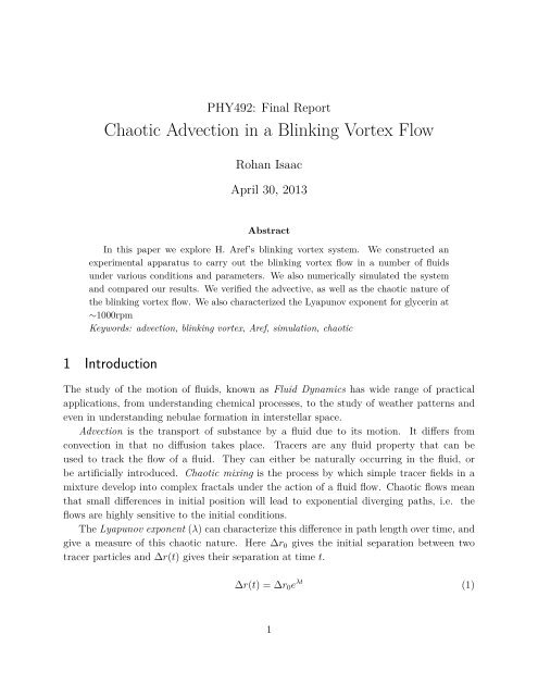
PHY492: Final ReportChaotic Advection in a Blinking Vortex FlowRohan IsaacApril 30, 2013AbstractIn this paper we explore H. Aref’s blinking vortex system. We constructed anexperimental apparatus to carry out the blinking vortex flow in a number of fluidsunder various conditions and parameters. We also numerically simulated the systemand compared our results. We verified the advective, as well as the chaotic nature ofthe blinking vortex flow. We also characterized the Lyapunov exponent for glycerin at∼1000rpmKeywords: advection, blinking vortex, Aref, simulation, chaotic1 IntroductionThe study of the motion of fluids, known as Fluid Dynamics has wide range of practicalapplications, from understanding chemical processes, to the study of weather patterns andeven in understanding nebulae formation in interstellar space.Advection is the transport of substance by a fluid due to its motion. It differs fromconvection in that no diffusion takes place. Tracers are any fluid property that can beused to track the flow of a fluid. They can either be naturally occurring in the fluid, orbe artificially introduced. Chaotic mixing is the process by which simple tracer fields in amixture develop into complex fractals under the action of a fluid flow. Chaotic flows meanthat small differences in initial position will lead to exponential diverging paths, i.e. theflows are highly sensitive to the initial conditions.The Lyapunov exponent (λ) can characterize this difference in path length over time, andgive a measure of this chaotic nature. Here ∆r 0 gives the initial separation between twotracer particles and ∆r(t) gives their separation at time t.∆r(t) = ∆r 0 e λt (1)1

Chaotic dynamics can help to understand mixing in fluids, which is a widespread andimportant process. Until recently it has been hard to make the connection between these twothings because of experimental limitations, but it is now possible to measure the stretchingprocess that allows the connection between chaos and mixing to be understood deeply.Another important quantity in studying fluids is the Reynolds number, a dimensionlessnumber that gives the measure of the ratio of inertial forces to viscous forces in a fluid.A Higher Reynolds number corresponds to more turbulent flow, while a lower Reynoldsnumber indicates a more laminar flow. A laminar flow occurs where fluid flows in parallellayers without disruption between layers.There are two main types of fluid mixing: Turbulent mixing and chaotic mixing. In bothprocesses, there is stretching and folding of fluid elements, which causes nearby points toseparate from each other irreversibly. Turbulent mixing is when random structures are producedby fluid instability at high Reynolds number (Re) and stretch and fold fluid elements.Chaotic mixing on the other hand is when laminar flows at modest Reynolds number canproduce complex distributions of the material.Only in recent years it been appreciated that a high Reynolds number (i.e. turbulentflow) is not necessary for complex particle trajectories in a fluid[4]. Hassan Aref in 1984showed that a simple fluid setup – a blinking vortex flow – could be used to create laminarfluid flow that becomes chaotic[1].2 ApplicationsMixing of fluids is highly important process for many chemical and industrial processes. Inmany cases however, mixing occurs in a confined space where there is not much room fordisorderly flow. In these kinds of cases, it is highly desirable to use a system such as Aref’sblinking vortex flow to efficiently mix two or more liquids while maintaining a laminar fluidflow. [3]Chaotic flows can observed in many natural processes and system; in environmentalflows such as the atmosphere and the ocean, where such irregular objects, like the unstablemanifolds, are traced out by advected impurities or by biological species. This can be usedto obtain new results in the field of chemical reactions and biological interactions of advectedactive tracers.In recent times, this chaotic advectation has been used in a number of fields to mix andblend materials together. The blinking vortex flow has been use in blending of polymers[8],creation of nanoscale structures[12] and more.2

3 TheoryThe blinking vortex system consists of two vortices that are equally spaced from the centerof a cylindrical container. A vortex is a region in a fluid where the fluid spins around animaginary axis. In the blinking vortex system, one of the vortices is turned on, while theother is off, and then they are reversed with the other being turned on while the first isturned off, and this cycle is repeated with a period T . This creates the blinking vortexeffect, as described by Aref in his 1984 paper[1].A two dimensional blinking vortex flow can be described by the following equations [6]Where x s is given byẋ = −Ay(2)x 2 s + y 2ẏ =Axx 2 s + y 2 (3)⎧⎨x + b if 0 < t < T/2x s =⎩x − b if T/2 < t < THere ẋ and ẏ give the x and y velocities of fluid around the two vortices centered at(±b, 0). One can see that since the x-velocity is dependent on the y-position and vice-versa,the motion of the fluid occurs in a circular fashion around the vortices. One can also notethat as the position from the vortex √ x 2 s + y 2 increases, the velocity decreases.For a single vortex, these equations reduce toẋ = −Ayx 2 + y , ẏ = 2(4)Axx 2 + y 2 (5)Converting this to polar coordinates with x = r cos θ and y = r sin θ, and squaring andadding together the two equations, we getẋ 2 + ẏ 2 = − A2 (x 2 + y 2 )(x 2 + y 2 ) 2 (6)Since x = r cos θ and y = r sin θ, ẋ = −r sin(θ) ˙θ and y = r cos(θ) ˙θSo, with v = ωr, and ω = ˙θ,ẋ 2 + ẏ 2 = r 2 ˙θ2 = A2r 2 (7)v =( Ar 2 )r = A r(8)3

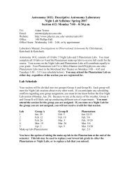
5 VDC Motor1N4004RELAY22 Ω0-40VArduinoDigital Out1 kΩ2N2222Arduino GNDGNDFigure 1: Circuit diagram showing DC motor controlled by Arduino via 5V relay (Based inpart on schematic on arduino.cc)4 Experimental SetupThis system was based in part on the experimental system described by the Applied Mathematicsdepartment at University of Colorado [7]. The experimental setup for my blinkingvortex consists of two glass rods (0.25in in diameter) as the two vortices. These rods areconnected to two high DC motors, with an input voltage rating of 0-18V with flexible joints.These joints are made by connecting the motor via a thin wooded dowel to the glass rod byheat shrinking layers of tubing over the connections, to create a flexible yet sturdy connection.The motors are connected to the variable DC output of a power supply. Two rheostatsare placed in series with the output to stabilize the voltage across the motors, which canfluctuate quite rapidly when switching between loads. Rheostats are used in place of standardresistors, because smaller resistors tend to burn out when the relatively large current flowsthrough them. The rheostats also help to control the current flowing to each motor andensuring that they both rotate at the same speed.The two motors are controlled through two 5V relay switches that are switched on andoff through the simple script running on the Arduino Mega 2560 board. The period of themotors can be changed with ease, but most of the cases we used a period T between 20 to60s. This range of values gives us sufficient time to record the movement created by onevortex before the effects of the other vortex are felt.4

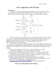
These glass rods were fully immersed in the fluid, which was placed in a 125mm diameterand 65mm deep Pyrex cylinder. 1 . Since the motion of the fluid could not be tracked directly,we introduced light tracer particles in the fluid that would not interfere with its motion.After a number of potential tracer particles, we settled on using small plastic spheres in therange of 2mm to 5mm. The motion of tracer particles was recorded from the bottom of theglass container using one a Logitech HD Pro C920 webcam connected to a computer throughLogger Pro.To increase the visibility of these tracer particles, we use a black background so that thelight tracer particles show up clearly. To reduce the friction of the glass rod on the supportsystem, we used a system of high-speed mechanical ball bearings that support each rod attwo points on either extreme of the rod (see figure ??). Care must be taken in aligning thesebearings so that it does not induce additional vibrations into the setup, especially at highspeed.To accurately detect the speed of the motors and thus the vortices, we researched andinvestigated a number of different methods. Measuring the ripple generated across the DCmotor due to the nature of the DC motor was one method, but did was not easy to processdue to the small amplitude of this signal. Another method was using a stroboscope on aflag on the rod, but this interfered with data collection with the webcam. A third methodswe tried was using slivering half the rod and measuring the current across the rod. Howeverdue to mechanical limitations, it was hard to maintain a steady contact between the wireand the rod, so we abandoned this method as well.Due the various drawbacks of these methods, the final method we used was that based ona photo-transistor. A bright LED is placed on one side of the rod and a photo-transistor isplaced on the other side, with the output connected to an oscilloscope. A opaque flag is placedon the rod. As the rod rotates, the flag interrupts the light falling on the photo-transistor,causing a spike in the output voltage. The frequency of these spikes is the frequency of thevortex. This signal was transmitted to an oscilloscope as well as an analog input port onthe Arduino board. We build two of such setups, one for each of the vortices in use.To process this data on the Arduino in real time, we used a simple algorithm whichcounted the number of times that the signal passed an experimentally determined threshold.If the signal passes the threshold nine times, it completes four periods (4T). Thus thefrequency of the motors is given bywhere rpm is the revolutions per minute.1 Courtesy of Dr. Anes Kovacevic, Chemistry Departmentf = 1 T Hz = 4 4 × 60Hz = rpm (9)(4T ) (4T )5

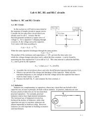
Figure 2: Full setup as of 2/27/2013(a) Glass rods supported by bearings.(b) Electronics control: Arduino Board and relaysFigure 3: Some parts of the experimental setup6

Figure 4: A periodic function passes a threshold 9 times over 4 wavelenghts.5 VPhototransistor5 VLED100 ΩTo Voltage Probe4.4 kΩFigure 5: Circuit setup of LED as well as phototransistor. The voltage probe lead is connectedto both an oscilloscope as well as analog input of the Arduino.Figure 6: Phototransistor based speed sensor.7

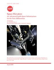
5 SimulationWe used a MATLAB program to numerically solve the coupled differential equations [?]describing the blinking vortex flow. Since the functions are defined piecewise, the differentialequations are solved in segments, and the final state of one solution is used as the initialcondition for the next segment to create a continuous solution. The differential equationsolver used was the inbuilt ode45(), which uses a variable step Runge-Kutta Methods tosolve the differential equations.The simulations tracks a single particle over time. To see the complete trace of theparticle over time, we conglomerated all these points to get figure 7, which describes thepath taken by a particle over some period. The details of the implementation can be seenin the appendix.Figure 7: Results of theoretical simulation for a particle over three periods. Note the colorsrefers to the motion undergone due to a particular vortex, in this case blue for the left andred for the right.6 DataTo recored data from this system we used a camera positioned below the setup. The camerarecorded video data which was analyzed with with aid of LoggerPro software. The motionof the particles was calibrated and traced with the aid of this software. The constant in8

Figure 8: Data or particle traced over about two periods for one of two particles in a blinkingvortex flow.equation A was determined using the fit for the equation of v vs r. Note that this constantdepends on the speed of the vortex, which can be changed.The frequency used in the system was usually between 1000 − 1200rpm. Though wetested frequency ranges between 500 rpm and 6000 rpm, we found that a lower frequencywas more stable. At higher frequencies the vibrations in the vortices build up and generatedbubble in the liquid used.The period used for the blinking vortex flow ranged from 1 s to 1 min, though for mostof our tests we used a period of 20s, i.e. 10 second for each motor. This value was mainlybased of obtaining sufficient data to record the position of the tracer particles using videodata at 15 frames per second.In most cases liquid used was glycerin, though we tested other fluids such as corn syrupand water. The corn syrup used had the highest viscosity, though it tend to form a thickhard film on top, which is why glycerin was used instead. water too was tried, but theviscosity of the water was so low that the vortices did not rotate the fluid at all.Before we began testing our blinking vortex flow, we wanted to check the validity of theequations that we assumed to be true. The first thing that we did was to verify that thev, velocity of the fluid (or in our case, a tracer particle in the fluid) decreased as 1/r as weincreased the radius from the vortex r. For a single vortex at a constant speed, we traced 8particles across multiple periods to find values for v and r. The results of this are shown infigure ??.9

0.060.05y(x) = (a / x) + ba = 0.0022077b = −0.037547R = 0.99513 (lin)0.04Velocity (m/s)0.030.020.0100.02 0.025 0.03 0.035 0.04 0.045 0.05 0.055 0.06Radius (m)Figure 9: Velocity as a function of radius for a single vortex rotating at 1200 rpm.??Another test that we conducted was to check the advective nature of this system. Ifit was truly advective, the system would return to its original state upon time reversal.Experimentally this means that if we reversed the motion of the vortices, a tracer particleTo accomplish this, we ran the system for a half integer period, such that the systemstopped spinning the same vortex that it started on. In this way, when running the secondtime, the reversing switch shown in figure 10 could be flipped such that the polarity of theDC motors would be reversed, and thus the whole system would run backwards.Theoretically these conditions would be exactly opposite to those in the forward direction,but due to mechanical limitations, it is not quite possible. Nevertheless we attempted to getas close as possible to the initial state in this manner. The results of our experiment areshown in figure 11, after 3 sets of rotations (1.5 periods).DC SourceDC MotorsSwitchFigure 10: Schematic for a reversing switch.10

80ForwardReverse60x-Position (mm)402000 5 10 15 20 25 30 35-20-40Time (s)Figure 11: The x-position of a particle upon reversal after 1.5 periods in a blinking vortexflow at ∼1000 rpm60ForwardReverse40y-Position (mm)200-200 5 10 15 20 25 30 35-40-60Time (s)Figure 12: The y-position of a particle upon reversal after 1.5 periods in a blinking vortexflow at ∼1000 rpm11

25Seperation (Δx) (mm)201510y = 0.4509e 1.0354xR² = 0.9527502 2.25 2.5 2.75 3 3.25 3.5 3.75 4Time (s)Figure 13: Exponential separation of two particles with similar initial conditions in a blinkingvortex flow with vortices spinning at 1000 rpm807060Seperation (Δx) (mm)504030201000 6 12 18Time (s)Figure 14: The seperation between the same two particles over a longer period of time.Notice that the exponential trend only continues for a short period at the fluid is contained.12

7 Results and ConclusionWe successfully constructed an experimental blinking vortex flow. We have measured positionof test tracer particles in a variety of fluids at various velocities over time. Theparameters of the blinking vortex system, such as period, size etc can easily be modified.The system has been shown to be advective in nature, as it can be reversed. We have alsoverified the equations that we assumed to be true, both using our numerical simulation, aswell as with experimental data.We have shown that the position of the particles deviates exponentially (figure 13) andhave characterized the Lyapunov exponent. For glycerin at ∼1000rpm this dimensionlessparameter is 1.0354. The separation over longer period is not exponential (as shown byfigure 14), and this is because the system is contained, and thus while the particles mightdiverge exponential over a small period, over longer timespan the separation between anytwo particles is limited and thus will oscillate over time.The blinking vortex system is thus a successful system with which to accomplish chaoticmixing. This is an advective system, where particles with small initial separation will divergeexponentially. It has a slew of applications, mainly in industry, for the mixing of materialsboth large and small.13

References[1] Aref, H. “Stirring by Chaotic Advection.” Journal of Fluid Mechanics 143 (1984): 1-21.Print.[2] Aref, H. “Chaotic Advection of Fluid Particles.” Philosophical Transactions of the RoyalSociety A: Mathematical, Physical and Engineering Sciences 333.1631 (1990): 273-88.Print.[3] Brehm, Denise. “Mixing Fluids Efficiently in Confined Spaces? Let Viscous FingersDo the Stirring.” Department of Civil and Environmental Engineering. MassachusettsInstitute of Technology, 12 May 2011. Web. 07 Feb. 2013.[4] Cartwright, Julyan HE, Mario Feingold, and Oreste Piro. “An introduction to chaoticadvection.” NATO ASI SERIES B PHYSICS 373 (1999): 307-342.[5] Karolyi, G., and T. Tel. “Chaotic Tracer Scattering and Fractal Basin Boundaries in aBlinking Vortex-sink System.” Physics Reports 290.1-2 (1997): 125-47. Print.[6] Nugent, C. R., W. M. Quarles, and T. H. Solomon. “Experimental Studies of PatternFormation in a Reaction-Advection-Diffusion System.” Physical Review Letters 93.21(2004): Print.[7] Schilt, Ryan, Joe Adams, and Anna Lieb. “Chaotic Advection and BlinkingVortices.” University of Colorado at Boulder. Department of Applied Mathematics,Web. 21 Jan. 2013. [8] Schut, Jan H. “Novel Melt Blending Technology Commercialized in Micro- andNanolayer Films.” Plastics Technology. Apr. 2009. Web. 21 Jan. 2013.[9] Skiadas, Christos H. “Exploring and simulating chaotic advection: A difference equationsapproach.” arXiv preprint nlin/0611036 (2006).[10] Solomon, T. “Lagrangian Chaos and Multiphase Processes in Vortex Flows.” Communicationsin Nonlinear Science and Numerical Simulation 8.3-4 (2003): 239-52. Print.[11] “Stirring Simulation.” University of Colorado at Boulder. Department of Applied Mathematics,Web. 21 Jan. 2013. .[12] Zumbrunnen, D. A., S. Inamdar, O. Kwon, and P. Verma. “Chaotic Advection as aMeans to Develop Nanoscale Structures in Viscous Melts.” Nano Letters 2.10 (2002):1143-148. Print.14

8 Appendix: Code/∗B l i n k i n gmotorsListing 1: ”Blink Flow”This s c r i p t turn one ouput high , then the o t h e r with a d e l a y o f 1 second .∗/// Pin 13 has an LED connected on most Arduino boards .// g i v e i t a name :// Output pins are 4 and 12i n t out1 = 4 ;i n t out2 = 1 2 ;// i n t = 13;// the s e t u p r o u t i n e runs once when you p r e s s r e s e t :void s e t u p ( ) {// i n i t i a l i z e the d i g i t a l pin as an output .pinMode ( out1 , OUTPUT) ;pinMode ( out2 , OUTPUT) ;}// the loop r o u t i n e runs over and over again f o r e v e r :void l o o p ( ) {d i g i t a l W r i t e ( out2 ,LOW) ;d i g i t a l W r i t e ( out1 , HIGH ) ; // turn the LED on (HIGH i s the v o l t a g e l e v e l )d e l a y ( 3 0 0 0 0 ) ; // wait f o r 10 secondsd i g i t a l W r i t e ( out1 , LOW) ; // turn the LED o f f by making the v o l t a g e LOWd i g i t a l W r i t e ( out2 , HIGH ) ;d e l a y ( 3 0 0 0 0 ) ; // wait f o r 10 seconds}Listing 2: ”Read Speed from Sensor”/∗ Read Analog Voltage o f one motor and p r i n t s frequency o fs i g n a l from analog i n p u t to s e r i a l v i a MegunoLink∗/// d i g i t a l output pins o f the two DC motor r e l a y c o n t r o l si n t motor1 = 4 ;i n t motor2 = 1 2 ;// middle o f v o l t a g e s i g n a l f o r frequency readingi n t t h r e s h o l d = 3 5 ;15

misc varsi n t f l a g = 0 , o l d f l a g = 0 , count = 0 ;unsigned long time , t1 ;double f r e q =0;// runs at r e s e tvoid s e t u p ( ) {// high output r a t e ( bps )S e r i a l . b e g i n ( 5 0 0 0 0 0 ) ;pinMode ( motor1 , OUTPUT) ;pinMode ( motor2 , OUTPUT) ;}void l o o p ( ) {d i g i t a l W r i t e ( motor1 , HIGH ) ; // s t a r t one motori n t s e n s o r V a l u e = analogRead (A0 ) ; // read analog pin 0// save o l d v a l u e f o r comparisono l d f l a g = f l a g ;// check i f c r o s s e si f ( s e n s o r V a l u e > t h r e s h o l d )f l a g = 1 ;e l s ef l a g = 0 ;// 9 f l a g s 4 w a v e l e n g h t si f ( f l a g != o l d f l a g ){i f ( count == 0){time = m i c r o s ( ) ;count++;}e l s e i f ( count == 8){t1 = m i c r o s ()− time ;f r e q = 240000000.0/(( double ) t1 ) ;S e r i a l . p r i n t l n ( f r e q ) ;count = 0 ;}e l s e{count++;}}// sendPlotData (” v o l t a g e ” , sensorValue ) ;16

sendPlotData ( ” f r e q ” , f r e q ) ; // rpm// sendPlotData (” time ” , t1 ) ;// sendPlotData (” count ” , count ) ;// sendPlotData (” f l a g ” , f l a g ) ;}// f l o a t v o l t a g e = sensorValue ; // ∗ ( 5 . 0 / 1 0 2 3 . 0 ) ; // s c a l e read v a l u e// S e r i a l . p r i n t l n ( v o l t a g e ) ;// sendPlotData (” v o l t a g e ” , v o l t a g e ) ;void sendPlotData ( S t r i n g seriesName , f l o a t data ){S e r i a l . p r i n t ( ”{” ) ;S e r i a l . p r i n t ( seriesName ) ;S e r i a l . p r i n t ( ” ,T, ” ) ;S e r i a l . p r i n t ( data ) ;S e r i a l . p r i n t l n ( ”}” ) ;}Listing 3: ”ODE Simulation”% BLINKING VORTEX FLOW% Simulate the two coupled d i f f e r e n t a l e q u a t i o n s f o r a b l i n k i n g v o r t e x% f l o w%% x ’ = −Ay/( xs ˆ2 + y ˆ2)% y ’ = Axs ˆ2/( xs ˆ2 + y ˆ2)%% xs = {% x − b i f 0 < t < T/2% x + b i f T/2 < t < T%% S o l v i n g Notes : Use ode45 , Solve f o r each l i t t l e i n t e r v a l , use f i n a l% c o n d i t i o n s f o r each next i n i t i a l c o n d i t i o nfunction s e n i o r o d e f u l l a n i m a t i o n ( )% Main Driver Function% I n i t i a l c o n d i t i o n st o t a l t i m e = [ 0 , 2 0 . 5 ] ;i n i t i a l p o s = [ 1 ; 1 ] ;g l o b a l A b ;A = 1 ; b = . 5 ;count = 1 ;f o r i =1:517

% S o l v e f i r s t s e t [ Function f ( t ) = x ( t ) , y ( t ) ][ t , f ]=ode45 ( @vortex1 , t o t a l t i m e , i n i t i a l p o s ) ;f o r j =1: s i z e ( f , 1 )p l o t ( f ( j , 1 ) , f ( j , 2 ) , ’ o ’ ) ;hold a l l ;M( count ) = getframe ;count = count +1;endf i n a l p o s =[ f ( end , 1 ) , f ( end , 2 ) ] ;% S t a r t second s e t with f i r s t i n i t i a l c o n d i t i o n s[ t , f ]=ode45 ( @vortex2 , t o t a l t i m e , f i n a l p o s ) ;endf o r k=1: s i z e ( f , 1 )p l o t ( f ( k , 1 ) , f ( k , 2 ) , ’ o ’ ) ;hold a l l ;M( count ) = getframe ;count = count +1;endi n i t i a l p o s = [ f ( end , 1 ) , f ( end , 2 ) ] ;endmovie (M, 1 , 1 0 0 ) ;function dydt=v o r t e x 1 ( t , y )% Vortex 1 ( r i g h t )% y (1) = x , y (2) = yg l o b a l A b ;dydt =[(A∗(−y ( 2 ) ) ) / ( ( y (1)−b )ˆ2 + y ( 2 ) ˆ 2 ) ; (A∗( y (1)−b ) ) / ( y (2)ˆ2+( y (1)−b ) ˆ 2 ) ] ;endfunction dydt=v o r t e x 2 ( t , y )% Vortex 2 ( l e f t )% y (1) = x , y (2) = yg l o b a l A b ;dydt =[(A∗(−y ( 2 ) ) ) / ( ( y (1)+b )ˆ2 + y ( 2 ) ˆ 2 ) ; (A∗( y (1)+b ) ) / ( y (2)ˆ2+( y (1)+b ) ˆ 2 ) ] ;end18