The Lognormal, Weibull, and Rayleigh Distributions A ... - Statistics

More documents

Recommendations

Info

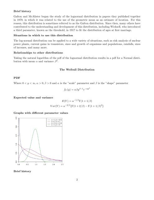
Brief historyGalton and McAlister began the study of the lognormal distribution in papers they published togetherin 1879, in which it was related to the use of the geometric mean as an estimate of location. For thisreason, this distribution is sometimes referred to as the Galton distribution. Since then, many others havecontributed to the understanding and development of this distribution, including Wicksell, who introduceda third parameter, known as the threshold, in 1917 to fit the distribution of ages at first marriage.Situations in which to use this distributionThe log-normal distribution can be applied to a wide variety of situations, such as risk analysis of nuclearpower plants, current gains in transistors, sizes and growth of organisms and populations, rainfalls, sizesof incomes, and many more.Relationships to other distributionsTaking the natural logarithm of the pdf of the lognormal distribution results in a pdf for a Normal distributionwith mean α and variance β 2 .The Weibull DistributionPDFWhere 0 < y < ∞, α > 0, β > 0 and α is the ”scale” parameter and β is the ”shape” parameterf Y (y) = αβy β−1 e −αyβExpected value and varianceE(Y ) = α −1/β Γ(1 + 1/β)V ar(Y ) = α −2/β {Γ(1 + 2/β) − Γ(1 + 1/β) 2 }Graphs with different parameter valuesBrief history2
The Weibull distribution is named after Waloddi Weibull in 1951 who was the first to describe and studyit in detail for its application to strength of material. However, this distribution was first discovered byFrechet in 1927 and first applied by material scientists Rosin and Rammer in 1933 to model the distributionof sizes of pulverized particles. Although it was originally proposed to model objects physical fatigue, itnow has many more applications.Situations in which to use this distributionThe Weibull distribution is most often used to model lifetimes and failure times. This may include reliability,failure rates, failure probability. The flexibility of this distribution allows for many practicalapplications. It can take into account increasing, decreasing, or constant failure rates. When β > 1 failurerate is increasing over time, and when β < 1 failure rate is decreasing over time, and β = 1 implies aconstant failure rate. This distribution is interesting because α, or characteristic life is set so 63.21% ofobjects fail at time x = α. For example, to study failure of an aluminum part α = 4, and for steel α = 3.The smaller the characteristic life is the more scatter of data there is around the model. This distributionis often applied in engineering to model physical degradation, as studied by Waloddi Weibull, and in seriessystems to model the weakest link. For example, this distribution is used by structural engineers to modeland predict fatigue and resulting cracks in airplanes.Relationships to other distributionsWhen failure rate is constant, i.e. β=1 then Weibull (α, 1) = Exponential (α)When β=2 then Weibull (α,β) = Rayleigh (α) = Chi (2, α) , where n=2The Rayleigh DistributionPDFf y (y) = y α 2 e −y22α 2 α > 0, 0 ≤ y < ∞= 0 elsewhereExpected value and variance√ πE[Y ] = α2Graphs with different parameter valuesBrief historyV ar[Y ] = 4 − π α 22John William Strutt, 3rd Baron Rayleigh (1842 - 1919) was a nineteenth- and twentieth-century Britishphysicist who discovered the pdf of Rayleigh arising in the study of wave motion, which earned him theNobel Prize for Physics. He also discovered Rayleigh scattering and predicted the existence of the surfacewaves now known as Rayleigh waves.Situations in which to use this distribution3
Page 1: The Lognormal, Weibull, and Rayleig

The Lognormal, Weibull, and Rayleigh Distributions A ... - Statistics

You also want an ePaper? Increase the reach of your titles

Delete template?

Save as template?