chapter 6 biomechanics of the musculoskeletal system

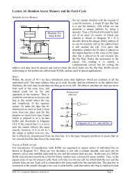
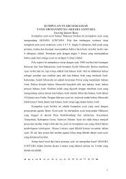
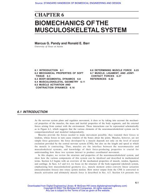
Source: STANDARD HANDBOOK OF BIOMEDICAL ENGINEERING AND DESIGNCHAPTER 6BIOMECHANICS OF THEMUSCULOSKELETAL SYSTEMMarcus G. Pandy and Ronald E. BarrUniversity of Texas at Austin6.1 INTRODUCTION 6.1 6.6 DETERMINING MUSCLE FORCE 6.236.2 MECHANICAL PROPERTIES OF SOFT 6.7 MUSCLE, LIGAMENT, AND JOINT-TISSUE 6.3 CONTACT FORCES 6.276.3 BODY-SEGMENTAL DYNAMICS 6.8 REFERENCES 6.326.4 MUSCULOSKELETAL GEOMETRY 6.116.5 MUSCLE ACTIVATION ANDCONTRACTION DYNAMICS 6.166.1 INTRODUCTIONAs the nervous system plans and regulates movement, it does so by taking into account the mechanicalproperties of the muscles, the mass and inertial properties of the body segments, and the externalforces arising from contact with the environment. These interactions can be represented schematicallyas in Figure 6.1, which suggests that the various elements of the neuromusculoskeletal system can becompartmentalized and modeled independently.Muscles provide the forces needed to make movement possible; they transmit their forces totendons, whose forces in turn cause rotation of the bones about the joints. Muscles, however, are notsimple force generators: the force developed by a muscle depends not only on the level of neuralexcitation provided by the central nervous system (CNS), but also on the length and speed at whichthe muscle is contracting. Thus, muscles are the interface between the neuromuscular andmusculoskeletal systems, and knowledge of their force-producing properties is crucial forunderstanding how these two systems interact to produce coordinated movement.In this chapter, we review the structure and properties of the neuromusculoskeletal system, andshow how the various components of this system can be idealized and described in mathematicalterms. Section 6.2 begins with an overview of the mechanical properties of muscle, tendon, ligament,and cartilage. In Secs. 6.3 and 6.4, we focus on the structure of the body-segmental (skeletal) system,emphasizing how musculoskeletal geometry (i.e., muscle moment arms) converts linear actuation(musculotendon forces) into rotary (joint) motion. How motor output from the CNS is converted tomuscle activation and ultimately muscle force is described in Sec. 6.5. Section 6.6 presents twoDownloaded from Digital Engineering Library @ McGraw-Hill (www.digitalengineeringlibrary.com)Copyright © 2004 The McGraw-Hill Companies. All rights reserved.Any use is subject to the Terms of Use as given at the website.6.1

BIOMECHANICS OF THE MUSCULOSKELETAL SYSTEM6.2 MECHANICS OF THE HUMAN BODYFIGURE 6.1 Schematic diagram showing how the human neuromusculoskeletal system can be compartmentalizedfor modeling purposes.Downloaded from Digital Engineering Library @ McGraw-Hill (www.digitalengineeringlibrary.com)Copyright © 2004 The McGraw-Hill Companies. All rights reserved.Any use is subject to the Terms of Use as given at the website.

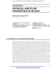
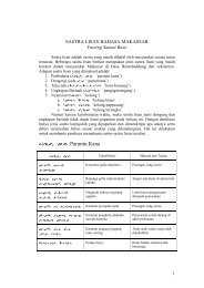
BIOMECHANICS OF THE MUSCULOSKELETAL SYSTEMBIOMECHANICS OF THE MUSCULOSKELETAL SYSTEM 6.3methods commonly used to determine musculoskeletal loading during human movement. Representative results of muscle, ligament, and joint-contact loading incurred during exercise and dailyactivity are given in Sec. 6.7.6.2 MECHANICAL PROPERTIES OF SOFT TISSUEWe focus our description of the mechanical properties of soft tissue on muscle, tendon, ligament, andcartilage. The structure and properties of bone are treated elsewhere in this volume.FIGURE 6.2 Structural organization of skeletal muscle from macro- tomicrolevel. Whole muscle (a), bundles of myofibrils (b), single myofibril(c), sarcomere (d), and thick (myosin) filament and thin (actin)filament (e). All symbols are defined in the text. [Modified from Enoka(1994).]Downloaded from Digital Engineering Library @ McGraw-Hill (www.digitalengineeringlibrary.com)Copyright © 2004 The McGraw-Hill Companies. All rights reserved.Any use is subject to the Terms of Use as given at the website.

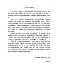
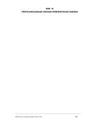
BIOMECHANICS OF THE MUSCULOSKELETAL SYSTEM6.4 MECHANICS OF THE HUMAN BODY6.2.1 MuscleGross Structure. Muscles are molecular machines that convert chemical energy into force. Individualmuscle fibers are connected together by three levels of collagenous tissue: endomysium, whichsurrounds individual muscle fibers; perimysium, which collects bundles of fibers into fascicles; andepimysium, which encloses the entire muscle belly (Fig. 6.2a). This connective tissue matrix connectsmuscle fibers to tendon and ultimately to bone.FIGURE 6.3 Force versus length curve for muscle, (a) Isometric force versus length properties when muscle is fully activated.Total = active + passive. (b) Isometric force versus length properties when activation level is halved. (c) Muscle force versusstriation spacing curve. Symbols defined in text. [Modified from Zajac and Gordon (1989) and from A. M. Gordon, A. F. Huxley,and F. J. Julian, Journal of Physiology, vol. 184, 1966.]Downloaded from Digital Engineering Library @ McGraw-Hill (www.digitalengineeringlibrary.com)Copyright © 2004 The McGraw-Hill Companies. All rights reserved.Any use is subject to the Terms of Use as given at the website.

BIOMECHANICS OF THE MUSCULOSKELETAL SYSTEMBIOMECHANICS OF THE MUSCULOSKELETAL SYSTEM 6.5Whole muscles are composed of groups of muscle fibers, which vary from 1 to 400 mm in lengthand from 10 to 60 µm in diameter. Muscle fibers, in turn, are composed of groups of myofibrils (Fig.6.2b), and each myofibril is a series of sarcomeres added end to end (Fig. 6.2c). The sarcomere isboth the structural and functional unit of skeletal muscle. During contraction, the sarcomeres areshortened to about 70 percent of their uncontracted, resting length. Electron microscopy andbiochemical analysis have shown that each sarcomere contains two types of filaments: thick filaments,composed of myosin, and thin filaments, containing actin (Fig. 6.2d). Near the center of thesarcomere, thin filaments overlap with thick filaments to form the AI zone (Fig. 6.2e).In the discussion below, the force-length and force-velocity properties of muscle are assumed tobe scaled-up versions of the properties of muscle fibers, which in turn are assumed to be scaled-upversions of properties of sarcomeres.Force-Length Property. The steady-state property of muscle is defined by its isometric force-lengthcurve, which is obtained when activation and fiber length are both held constant. When a muscle isheld isometric and is fully activated, it develops a steady force. The difference in force developedwhen the muscle is activated and when the muscle is passive is called the active muscle force (Fig.6.3a). The region where active muscle force is generated is (nominally), whereis the length at which active muscle force peaks; that is, when ; is called muscle fiberresting length or optimal muscle fiber length and is the maximum isometric force developed by themuscle (Zajac and Gordon, 1989). In Fig. 6.3a passive muscle tissue bears no force at length . Theforce-length property of muscle tissue that is less than fully activated can be considered to be ascaled-down version of the one that is fully activated (Fig. 6.3b). Muscle tissue can be less than fullyactivated when some or all of its fibers are less than fully activated.The shape of the active force-length curve (Fig. 6.3) is explained by the experimental observationthat active muscle force varies with the amount of overlap between the thick and thin filaments withina sarcomere (see also “Mechanism of Muscle Contraction” in Sec. 6.5.2). The muscle force versusstriation spacing curve given in Fig. 6.3c shows that there is minimal overlap of the thick and thinfilaments at a sarcomere length of 3.5 µm, whereas at a length of about 2.0 µm there is maximumFIGURE 6.4 Force versus velocity curve for muscle when (a) muscle tissue is fully activated and (b) activation is halved. Symbols defined in text.[Modified from Zajac and Gordon (1989).]Downloaded from Digital Engineering Library @ McGraw-Hill (www.digitalengineeringlibrary.com)Copyright © 2004 The McGraw-Hill Companies. All rights reserved.Any use is subject to the Terms of Use as given at the website.

BIOMECHANICS OF THE MUSCULOSKELETAL SYSTEM6.6 MECHANICS OF THE HUMAN BODYFIGURE 6.5 Structural organization of tendon or ligament from macro- tomicrolevel. Modified from Enoka (1994).overlap between the cross-bridges. As sarcomere length decreases to 1.5 µm, the filaments slidefarther over one another, and the amount of filament overlap again decreases. Thus, muscle forcevaries with sarcomere length because of the change in the number of potential cross-bridgeattachments formed.Force-Velocity Property. When a constant load is applied to a fully activated muscle, the muscle willshorten (concentric contraction) if the applied load is less than the maximum isometric force developedby the muscle for the length at which the muscle is initially contracting. If the applied load isgreater than the muscle’s maximum isometric force at that length, then the muscle will lengthen(eccentric contraction). From a set of length trajectories obtained by applying different loads toshortening and lengthening muscle, an empirical force-velocity relation can be derived for anymuscle length l M (Fig. 6.4a). At the optimal fiber length , a maximum shortening velocity v max , canbe defined such that the muscle tissue cannot resist any load even when it is fully activated (Fig.6.4a). As with the force-length curve, it is commonly assumed that the force-velocity relation scalesproportionally with activation, although some studies have found that the maximum shorteningvelocity v max is also a function of muscle length (Fig. 6.4b).Downloaded from Digital Engineering Library @ McGraw-Hill (www.digitalengineeringlibrary.com)Copyright © 2004 The McGraw-Hill Companies. All rights reserved.Any use is subject to the Terms of Use as given at the website.

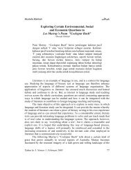
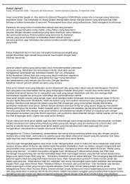
BIOMECHANICS OF THE MUSCULOSKELETAL SYSTEMBIOMECHANICS OF THE MUSCULOSKELETAL SYSTEM 6.7FIGURE 6.6 Force versus length curves for human medial patellar tendon, gracilis tendon, fascia latatendon, and the anterior cruciate ligament.6.2.2 Tendon and LigamentGross Structure. Tendon connects muscle to bone, whereas ligament connects bone to bone. The maindifference between the structure of tendon and ligament is the organization of the collagen fibril. Intendon, the fibrils are arranged longitudinally in parallel to maximize the resistance to tensile (pulling)forces exerted by muscle. In ligament, the fibrils are generally aligned in parallel with someoblique or spiral arrangements to accommodate forces applied in different directions.Tendons and ligaments are dense connective tissues that contain collagen, elastin, proteoglycans,water, and fibroblasts. Approximately 70 to 80 percent of the dry weight of tendon and ligamentconsists of Type I collagen, which is a fibrous protein. Whole tendon is composed of bundles offascicles, each made up in turn of bundles of fibrils (Fig. 6.5). The collagen fibril is the basic loadbearingunit of tendon and ligament. The fibril consists of bundles of microfibrils held together bybiochemical bonds (called cross-links) between the collagen molecules. Because these cross-links bindthe microfibrils together, the number and state of the cross-links are thought to have a significanteffect on the strength of the connective tissue.Stress-Strain Property. When a tensile force is applied to tendon or ligament at its resting length, thetissue stretches. Figure 6.6 shows the force-length curves for three different muscle tendons and oneknee ligament found in humans. These data show that the medial patellar tendon is much strongerthan either the gracilis or fascia lata tendons. Interestingly, the anterior cruciate ligament is alsostronger than the gracilis and fascia lata tendons, and is slightly more compliant as well.Force-length curves can be normalized to subtract out the effects of geometry; thus, force can benormalized by dividing by the cross-sectional area of a tissue, while length can be normalized bydividing by the initial length of the tendon or ligament. The resulting stress-strain curve displays threecharacteristic regions: the toe region, the linear region, and the failure region (Fig. 6.7). The toeregion corresponds to the initial part of the stress-strain curve and describes the mechanical behaviorof the collagen fibers as they are being stretched and straightened from the initial, resting zigzagpattern. The linear region describes the elastic behavior of the tissue, and the slope of the curve in thisregion represents the elastic modulus of the tendon or ligament. The failure region describes plasticchanges undergone by the tissue, where a small number of fibrils first rupture, followed by ultimatefailure of the whole tissue.Downloaded from Digital Engineering Library @ McGraw-Hill (www.digitalengineeringlibrary.com)Copyright © 2004 The McGraw-Hill Companies. All rights reserved.Any use is subject to the Terms of Use as given at the website.

BIOMECHANICS OF THE MUSCULOSKELETAL SYSTEMBIOMECHANICS OF THE MUSCULOSKELETAL SYSTEM 6.9FIGURE 6.8 Number of degrees of freedom (dof) of a joint. See text for explanation. [Modified from Zajac and Gordon (1989).]relative to the other (θ 1 , θ 2 , θ 3 in Fig. 6.8a), and 3 associated with the position of a point on onesegment relative to the other segment (x, y, z in Fig. 6.8a).In coordination studies, models of joints are kept as simple as possible. In studies of walking, forexample, the hip is often assumed to be a ball-and-socket joint, with the femur rotating relative to thepelvis only (Anderson and Pandy, 2001b). Thus, the position of the femur relative to the pelvis canbe described by three angles, as illustrated in Fig. 6.8b. In jumping, pedaling, and rising from a chair,the hip may even be assumed to be a simple hinge joint, in which case the position of the femurrelative to the pelvis is described by just one angle, as shown in Fig. 6.8c.Contact with the environment serves to constrain the motion of the body segments during a motortask. Consider the task of vertical jumping as illustrated in Fig. 6.9. Assuming that movement of thebody segments is constrained to the sagittal plane, Figure 6.9a indicates that the motor task has 6 dofwhen the body is in the air (x p , y p , which specify the position of the metatarsals plus θ 1 , θ 2 , θ 3 , θ 4 , whichspecify the orientation of the foot, shank, thigh, and trunk, respectively). When the metatarsals touchthe ground, only 4 generalized coordinates are needed to specify the position and orientation of thebody segments relative to any point on the ground, and accordingly the motor task has only 4 dof(Figure 6.9b). Similarly, when the feet are flat on the ground, the number of generalized coordinatesand the number of dof are each correspondingly reduced by 1 (Fig. 6.9c).6.3.2 Equations of MotionOnce a set of generalized coordinates has been specified and a kinematic model of the motor taskhas been defined, the governing equations of motion for the motor task can be written. Thenumber of dynamical equations of motion is equal to the number of dof of the motor task; thus, ifthe number of dof changes during a motor task (see Fig. 6.9), so too will the structure of theequations of motion.Different methods are available to derive the dynamical equations of motion for a motor task. Inthe Newton-Euler method (Pandy and Berme, 1988), free-body diagrams are constructed to show theexternal forces and torques acting on each body segment. The relationships between forces and linearDownloaded from Digital Engineering Library @ McGraw-Hill (www.digitalengineeringlibrary.com)Copyright © 2004 The McGraw-Hill Companies. All rights reserved.Any use is subject to the Terms of Use as given at the website.

BIOMECHANICS OF THE MUSCULOSKELETAL SYSTEM6.10 MECHANICS OF THE HUMAN BODYFIGURE 6.9 Number of dof of a motor task such as landing from a vertical jump. [Modified from Zajac and Gordon (1989).]accelerations of the centers of mass of the segments are written according to Newton’s second law (ΣF= ma), and the relationships between torques and angular accelerations of the segments are writtenusing Ruler’s equation (ΣT = Iα).The Newton-Euler method is well suited to a recursive formulation of the kinematic and dynamicequations of motion (Pandy and Berme, 1988); however, its main disadvantage is that all of theintersegmental forces must be eliminated before the governing equations of motion can be formed. Inan alternative formulation of the dynamical equations of motion, Kane’s method (Kane andLevinson, 1985), which is also referred to as Lagrange’s form of D’Alembert’s principle, makesexplicit use of the fact that constraint forces do not contribute directly to the governing equations ofmotion. It has been shown that Kane’s formulation of the dynamical equations of motion iscomputationally more efficient than its counterpart, the Newton-Euler method (Kane and Levinson,1983).The governing equations of motion for any multijoint system can be expressed aswhere q, , = vectors of the generalized coordinates, velocities, accelerations, respectivelyM(q) = system mass matrixM(q) = vector of inertial forces and torquesC(q) 2= vector of centrifugal and Coriolis forces and torquesG(q) = vector of gravitational forces and torquesR(q) = matrix of muscle moment arms (see Sec. 6.4.3)F MT = vector of musculotendon forcesR(q)F MT = vector of musculotendon torquesE(q, ) = vector of external forces and torques applied to the bodyby the environment(6.1)Downloaded from Digital Engineering Library @ McGraw-Hill (www.digitalengineeringlibrary.com)Copyright © 2004 The McGraw-Hill Companies. All rights reserved.Any use is subject to the Terms of Use as given at the website.

BIOMECHANICS OF THE MUSCULOSKELETAL SYSTEMBIOMECHANICS OF THE MUSCULOSKELETAL SYSTEM 6.11If the number of dof of the motor task is greater than, say, 4, a computer is needed to obtain Eq. (6.1)explicitly. A number of commercial software packages are available for this purpose includingAUTOLEV by On-Line Dynamics Inc., SD/FAST by Symbolic Dynamics Inc., ADAMS by MechanicalDynamics Inc., and DADS by CADSI.6.4 MUSCULOSKELETAL GEOMETRY6.4.1 Modeling the Paths of Musculotendinous ActuatorsTwo different methods are used to model the paths of musculotendinous actuators in the body: thestraight-line method and the centroid-line method. In the straight-line method, the path of a musculotendinousactuator (muscle and tendon combined) is represented by a straight line joining thecentroids of the tendon attachment sites (Jensen and Davy, 1975). Although this method is easy toimplement, it may not produce meaningful results when a muscle wraps around a bone or anothermuscle (see Fig. 6.10). In the centroid-line method, the path of the musculotendinous actuator isrepresented as a line passing through the locus of cross-sectional centroids of the actuator (Jensen andDavy, 1975). Although the actuator’s line of action is represented more accurately in this way, thecentroid-line method can be difficult to apply because (1) it may not be possible to obtain thelocations of the actuator’s cross-sectional centroids for even a single position of the body, and (2)even if an actuator’s centroid path is known for one position of the body, it is practically impossibleto determine how this path changes as body position changes.One way of addressing this problem is to introduce effective attachment sites or via points atspecific locations along the centroid path of the actuator. In this approach, the actuator’s line of actionis defined by either straight-line segments or a combination of straight-line and curved-line segmentsbetween each set of via points (Brand et al., 1982; Delp et al., 1990). The via points remain fixedrelative to the bones even as the joints move, and muscle wrapping is taken into account by makingthe via points active or inactive, depending on the configuration of the joint. This method worksquite well when a muscle spans a 1-dof hinge joint, but it can lead to discontinuities in the calculatedvalues of moment arms when joints have more than 1 rotational dof (Fig. 6.10).6.4.2 Obstacle-Set MethodAn alternative approach, called the obstacle-set method, idealizes each musculotendinous actuator asa frictionless elastic band that can slide freely over the bones and other actuators as the configurationof the joint changes (Garner and Pandy, 2000). The musculotendinous path is defined by a series ofstraight-line and curved-line segments joined together by via points, which may or may not be fixedrelative to the bones.To illustrate this method, consider the example shown in Fig. 6.11, where the path of the actuator isconstrained by a single obstacle, which is fixed to bone A. (An obstacle is defined as any regular-shapedrigid body that is used to model the shape of a constraining anatomical structure such as a bone oranother muscle.) The actuator’s path is defined by the positions of the five fixed via points and thepositions of the two obstacle via points. (A fixed via point remains fixed in a bone reference frame andis always active; an obstacle via point is not fixed in any reference frame, but is constrained to moveon the surface of an underlying obstacle.) Via points P 1 and P 2 are fixed to bone A, while S 1 , S 2 , and S 3are fixed to bone B. For a given configuration of the joint, the paths of all segments of the muscle areknown, except those between the bounding-fixed via points, P 2 and S 3 . The path of the actuator isknown once the positions of the obstacle via points Q and T have been found.Figure 6.12 shows a computational algorithm that can be used to model the centroid path of amusculotendinous actuator for a given configuration of the joints in the body. There are four steps inthe computational algorithm. Given the relative positions of the bones, the locations of all fixed viaDownloaded from Digital Engineering Library @ McGraw-Hill (www.digitalengineeringlibrary.com)Copyright © 2004 The McGraw-Hill Companies. All rights reserved.Any use is subject to the Terms of Use as given at the website.

BIOMECHANICS OF THE MUSCULOSKELETAL SYSTEM6.12 MECHANICS OF THE HUMAN BODYFIGURE 6.10 (a) Comparison of moment arms for the long head of triceps obtained using thestraight-line model (Straight), fixed-via-point model (Fixed), and the obstacle-set model(Obstacle). For each model, the moment arms were calculated over the full range of elbowflexion, with the humerus positioned alongside the torso in neutral rotation (solid lines) andin 45° internal rotation (dotted lines). (b) Expanded scale of the graph above, where themoment arms obtained using the fixed-via-point and obstacle-set models are shown near theelbow flexion angle where the muscle first begins to wrap around the obstacle (cylinder)placed at the elbow [see part (a)]. The fixed-via-point model produces a discontinuity inmoment arm when the shoulder is rotated 45° internally (Fixed, dotted line). [Modified fromGarner and Pandy (2000).]points are known and can be expressed in the obstacle reference frame (Fig. 6.12, Step 1). Thelocations of the remaining via points in the actuator’s path, the obstacle via points, can be calculatedusing one or more of the four different obstacle sets given in Appendices C to F in Garner and Pandy(2000) (Fig. 6.12, Step 2). Once the locations of the obstacle via points are known, a check is madeto determine whether any of these points should be inactive (Fig. 6.12, Step 3). If an obstacle viapoint should be inactive, it is removed from the actuator’s path and the locations of the remainingDownloaded from Digital Engineering Library @ McGraw-Hill (www.digitalengineeringlibrary.com)Copyright © 2004 The McGraw-Hill Companies. All rights reserved.Any use is subject to the Terms of Use as given at the website.

BIOMECHANICS OF THE MUSCULOSKELETAL SYSTEMBIOMECHANICS OF THE MUSCULOSKELETAL SYSTEM 6.13FIGURE 6.11 Schematic of a hypothetical muscle (a) represented by theobstacle-set model [(b) and (c)]. The muscle spans a single joint that connectsbones A and B. Reference frames attached to the bones are used todescribe the position and orientation of the bones relative to each other.At certain joint configurations, the muscle contacts the bones and causesthe centroid path of the muscle to deviate from a straight line (a). Themuscle path is modeled by a total of seven via points; five of these arefixed via points (P 1 , P 2 , S 1, S 2 , S 3 ); the remaining two are obstacle via points(Q, T), which move relative to the bones and the obstacle. Points P1 and S1are the origin and insertion of the muscle. Points P 2 and S 3 are boundingfixedvia points. The obstacle is shown as a shaded circle, which representsthe cross section of a sphere or cylinder. An obstacle reference framepositions and orients the obstacle relative to the bones. The obstacle ismade larger than the cross sections of the bones in order to account for thethickness of the muscle belly. The obstacle set is defined by the obstacle,the four via points (P 2 , Q, T, S 3 ), and the segments of the muscle pathbetween the via points P 2 and S 3 . At some joint configurations, the musclepath can lose contact with the obstacle, and the obstacle via points thenbecome inactive (c). See Garner and Pandy (2000) for details of the obstacle-setmethod. [Modified from Garner and Pandy (2000).]obstacle via points are then recomputed (Fig. 6.12, repeat Steps 2 and 3). Finally, the lengths of thesegments between all of the active via points along the actuator’s path are computed (Fig. 6.12, Step 4).The computational algorithm shown in Fig. 6.12 was used to model the paths of the triceps brachiimuscle in the arm (Garner and Pandy, 2000). The muscle was separated into three segments: theDownloaded from Digital Engineering Library @ McGraw-Hill (www.digitalengineeringlibrary.com)Copyright © 2004 The McGraw-Hill Companies. All rights reserved.Any use is subject to the Terms of Use as given at the website.

BIOMECHANICS OF THE MUSCULOSKELETAL SYSTEM6.14 MECHANICS OF THE HUMAN BODYFIGURE 6.12 Flowchart of the obstacle-set algorithm. See text for details.Downloaded from Digital Engineering Library @ McGraw-Hill (www.digitalengineeringlibrary.com)Copyright © 2004 The McGraw-Hill Companies. All rights reserved.Any use is subject to the Terms of Use as given at the website.

BIOMECHANICS OF THE MUSCULOSKELETAL SYSTEMBIOMECHANICS OF THE MUSCULOSKELETAL SYSTEM 6.15medial, lateral, and long heads (Fig. 6.13). Themedial head [Fig. 6.13 (1)] and lateral head[Fig. 6.13 (3)] were each modeled by a singlecylinderobstacle set (not shown in Fig. 6.13).The long head [Fig. 6.13 (2)] was modeled by adouble-cylinder obstacle set as illustrated. Thelocations of the attachment sites of each musclesegment and the locations and orientations ofthe obstacles were chosen to reproduce thecentroid paths of each head as accurately aspossible. The geometry of the bones and thecentroid paths of the muscle segments wereobtained from three-dimensional reconstructionsof high-resolution medical images obtainedfrom the National Library of Medicine’s VisibleHuman Male dataset (Garner and Pandy, 2001).Because the path of a muscle is not improperlyconstrained by contact with neighboringmuscles and bones, the obstacle-set methodproduces not only accurate estimates of musclemoment arms, but also smooth moment armjointangle curves, as illustrated in Fig. 6.10.6.4.3 Muscle Moment ArmsMuscles develop forces and cause rotation of thebones about a joint. The tendency of a musculotendinousactuator to rotate a bone about a jointis described by the actuator’s moment arm. Twomethods are commonly used to measure the momentarm of an actuator—the geometric methodand the tendon excursion method.In the geometric method, a finite center ofrotation is found by x-rays, computedtomography, or magnetic resonance imaging,and the moment arm is found by measuring theperpendicular distance from the joint center tothe line of action of the muscle (Jensen andDavy, 1975). In the tendon excursion method,the change in length of the musculotendinousFIGURE 6.13 Posterolateral view of the obstacle-set modelused to represent the paths of the triceps brachii in a model ofthe arm. The medial head (1) and lateral head (3) were eachmodeled by a single-cylinder obstacle set, which is not shownin the diagram. The long head (2) was modeled by a doublecylinderobstacle set as illustrated here. The locations of theattachment sites of the muscle and the locations and orientationsof the obstacles were chosen to reproduce the centroidpaths of each portion of the modeled muscle. The geometry ofthe bones and the centroid paths of the muscles were based onthree-dimensional reconstructions of high-resolution medicalimages obtained from the National Library of Medicine’sVisible Human Male dataset. [Modified from Garner andPandy (2000).]actu ator is measured as a function of the joint angle, and the moment arm is obtained by evaluatingthe slope of the actuator-length versus joint-angle curve over the full range of joint movement (Anet al., 1983).Consider two body segments, A and B, which articulate at a joint (Fig. 6.14). By considering theinstantaneous power delivered by a musculotendinous actuator to body B, it can be shown that themoment arm of the actuator can be written as (Pandy, 1999):where F M = musculotendinous force directed from the effective insertion of the actuator on bodyB (point Q) to the effective origin of the actuator on body A (point P)= unit vector that specifies the direction of the angular velocity of body B in bodyA [i.e., parallel to the instantaneous axis of rotation (ISA) of body B relative tobody A](6.2)Downloaded from Digital Engineering Library @ McGraw-Hill (www.digitalengineeringlibrary.com)Copyright © 2004 The McGraw-Hill Companies. All rights reserved.Any use is subject to the Terms of Use as given at the website.

BIOMECHANICS OF THE MUSCULOSKELETAL SYSTEM6.16 MECHANICS OF THE HUMAN BODYr OQ = position vector directed from any point O on theISA to any point Q on the line of action of theactuator between its origin and insertion sites= unit vector in the direction of the actuator forceF M (see Fig. 6.14)In Eq. (6.2), r M is the moment-arm vector, which is equal to themoment of the musculotendinous force per unit of musculotendinousforce. The direction of the moment-arm vector is along theinstantaneous axis of rotation of the body B relative to body Awhose direction is described by the unit vector .In the tendon excursion method, Euler’s theorem on rotation isused to define an equivalent relation for the moment arm of amusculotendinous force. Thus, if every change in the relativeorientation of body A and body B can be produced by means of asimple rotation of B in A about the ISA, then the moment arm ofa musculotendinous force can also be written as (Pandy, 1999):(6.3)FIGURE 6.14 Two bodies, A and B,shown articulating at a joint. Body Ais fixed in an inertial reference frame,and body B moves relative to it. Thepath of a generic muscle is representedby the origin S on B, the insertion N onA, and three intermediate via points P,Q, and R. Q and R are via points arisingfrom contact of the muscle path withbody B. Via point P arises from contactof the muscle path with body A. TheISA of B relative to A is defined by theangular velocity vector of B in A ( A ω B ).[Modified from Pandy (1999).]where l M = length of the musculotendinous actuator betweenthe effective origin and insertion sites (P to Qin Fig. 6.14)θ = angle associated with the simple rotation of bodyB about the ISA= total derivative of musculotendinous length withrespect to the angle of rotation θ ofbody B relative to body AEquations (6.2) and (6.3) have the same geometric interpretation:the moment arm of a muscle force r M , given either by ·from Eq (6.2) or by dl M /dθ from Eq. (6.3), is equal tothe perpendicular (shortest) distance between the ISA of B relativeto A and the line of action of the muscle force, multiplied bythe sine of the angle between these two lines (Pandy, 1999).6.5 MUSCLE ACTIVATION AND CONTRACTION DYNAMICS6.5.1 Muscle Activation DynamicsNeural Excitation of Muscle. Voluntary contraction of human muscle initiates in the frontal motorcortex of the brain, where impulses from large pyramidal cells travel downward through corticospinaltracts that lead out to peripheral muscles. These impulses from the motor cortex are called actionpotentials, and each impulse is associated with a single motor neuron. The principle structure of a motorneuron is shown in Fig. 6.15. The action potential initiates in the cell body, or soma, and travels downa long efferent trunk, called the axon, at a rate of about 80 to 120 m/s. The action potential waveformis the result of a voltage depolarization-repolarization phenomenon across the neuron cell membrane.The membrane ionic potential at rest is disturbed by a surrounding stimulus, and Na + ions are allowedto momentarily rush inside. An active transport mechanism, called the Na + -K + pump, quickly returns theDownloaded from Digital Engineering Library @ McGraw-Hill (www.digitalengineeringlibrary.com)Copyright © 2004 The McGraw-Hill Companies. All rights reserved.Any use is subject to the Terms of Use as given at the website.

BIOMECHANICS OF THE MUSCULOSKELETAL SYSTEMBIOMECHANICS OF THE MUSCULOSKELETAL SYSTEM 6.17transmembrane potential to rest. This sequence of events,which lasts about 1 ms, stimulates a succession of nerveimpulses or waves that eventually reach muscle tissue.When an impulse reaches the muscle, it conducts overmuscle tissue as a motor unit action potential (MUAP).Motor unit action potentials can have a variety of generalshapes (Fang et al., 1997), as depicted in Fig. 6.16.FIGURE 6.15 Motor neuron. (A) cell body, (B) axon,(C) neuromuscular junction, and (D) muscle fiber. Theaction potential travels downward, from the cell bodytowards the neuromuscular junction.FIGURE 6.16 Representative motor unit action potentials (MUAPs).(a) Change in shapes due to increase in stimulation, (b) Sequence ofMUAPs during voluntary contraction. [Source: Fang et al., 1997.]The connecting site between the motor neuron andthe muscle is called the neuromuscular junction. Onemotor neuron can have branches to many muscle fibers,and these together are called a motor unit. Whenthe nerve impulse reaches the end of the nerve fiber, aneurotransmitter called acetylcholine is released into themotor end plate of the muscle. This in turn causes therelease of Ca ++ ions deep into the muscle fiber. The presenceof Ca ++ ions causes cross-bridges to be formed betweenactin and myosin filaments in the sarcomeres. The actin filaments slide inward along themyosin filaments, causing the muscle fiber to contract.In addition to cortical motor neurons, control of the musculosketal system also relies on afferentreceptors or sensory neurons that carry information from the periphery to the brain or spinal cord.The simplest nerve pathways lead directly from sensory neurons to motor neurons, and are known asreflex arcs. One such example is the withdrawal reflex. When skin receptors sense something is hot orsharp (a pin prick, for example), a sensory impulse is sent to the spinal cord, where an interneuronintegrates the information and relays it to a motor neuron. The motor neuron in turn transmits asignal to the appropriate flexor muscle, which contracts and thus completes the reflex loop.Muscle Electromyography. While motor unit action potentials form the cellular origin for muscleactivation, they are normally not observable in routine clinical applications. The electromyogram(EMG) is the primary tool to study muscle activation in clinical and research settings using bothsurface and indwelling electrodes (Basmajian and DeLuca, 1985). The electromyogram is the summationof all motor unit action potentials at a given location during muscle contraction. Hence itrepresents a “gross” measure of the strength of a muscle contraction, since the number of musclefibers contracting is directly related to the number of motor units firing.Downloaded from Digital Engineering Library @ McGraw-Hill (www.digitalengineeringlibrary.com)Copyright © 2004 The McGraw-Hill Companies. All rights reserved.Any use is subject to the Terms of Use as given at the website.

BIOMECHANICS OF THE MUSCULOSKELETAL SYSTEM6.18 MECHANICS OF THE HUMAN BODYThe EMG appears as a random series of bursts that represent periods of muscle contraction andrelaxation. Figure 6.17 shows a series of EMG bursts. The EMG signal is acquired by both invasiveand noninvasive techniques. In invasive detection, a needle or fine wire is inserted directly into themuscle to a depth of several centimeters. In noninvasive techniques, also known as surfaceelectromyography, a recording electrode is pasted onto the skin approximately halfway between themuscle’s origin and insertion sites. In either case, because of the low voltage of the EMG signal (100µV to several millivolts), some amplification of the signal is needed before it enters the digital datacollection system. In addition, to reduce unwanted noise in the signal, an analog filter with passbandof 20 to 500 Hz should be used. This necessitates a typical digital sampling rate of 1000 Hz.Subsequent reduction of noise in the EMG signal can be handled computationally by digital filtering(Barr and Chan, 1986). A set of 16 recommendations for EMG acquisition and processing has beenpresented by DeLuca (1997).The EMG is analyzed in both the amplitude and frequency domains. For amplitude analysis, themost common processing technique is to compute a running root-mean-square (rms) of the signal.Over a short observational period T, the rms of the signal x(t) can be expressed as(6.4)In discrete form, over N contiguous samples, the rms can be expressed as:FIGURE 6.17 Two representative EMG bursts from the biceps muscle during an elbow flexion maneuver.Downloaded from Digital Engineering Library @ McGraw-Hill (www.digitalengineeringlibrary.com)Copyright © 2004 The McGraw-Hill Companies. All rights reserved.Any use is subject to the Terms of Use as given at the website.

BIOMECHANICS OF THE MUSCULOSKELETAL SYSTEMBIOMECHANICS OF THE MUSCULOSKELETAL SYSTEM 6.19(6.5)An alternative, but similar, approach to EMG amplitude analysis is to rectify and then integrate thesignal over the short period T (called integrated EMG, or IEMG). This approach has the advantage inthat a simple electronic circuit can be used and no numerical computation is necessary. In either case,the objective is to obtain an estimation of the underlying muscle contraction force, which is roughlyproportional to the EMG rms or IEMG. In recent efforts to use the EMG signal as a myoelectric controlsignal (Evans et al., 1994), a three-stage digital processing approach has arisen; it is illustrated in Fig.6.18. The process consists of (1) band-pass filtering (20 to 200 Hz) of the signal, (2) fullwaverectification, and (3) low-pass filtering (10-Hz cutoff) to produce a smooth signal.In the frequency domain, the most common tool is to apply a fast Fourier transform (FFT) to theEMG signal. A typical result is shown in Fig. 6.19. One can see that most of the power in the signalis confined to the 20- to 200-Hz range, and that the center frequency or mean power point istypically below 100 Hz. One use of EMG frequency analysis is in the study of muscle fatigue. It hasbeen shown that as the muscle fatigues, the median power frequency of the EMG shifts downward(Big-land-Ritchie et al., 1983).Modeling Activation Dynamics. As noted is Sec. 6.5.1 (“Neural Excitation of Muscle”), musclecannot activate or relax instantaneously. The delay between excitation and activation (or the developmentof muscle force) is due mainly to the time taken for calcium pumped out of the sarcoplasmicreticulum to travel down the T-tubule system and bind to troponin (Ebashi and Endo, 1968). Thisdelay is often modeled as a first-order process (Zajac and Gordon 1989; Pandy et al., 1992):(6.6)where u represents the net neural drive to muscle and a m the activation level. Other forms of thisrelation are also possible; for example, an equation that is linear in the control u has been used tosimulate jumping (Pandy et al., 1990) as well as pedaling (Raasch et al., 1997). Implicit in theformulation of Eq. (6.6) is the assumption that muscle activation depends only on a single variable u.Other models assume that a depends on two inputs, u 1 and u 2 say, which represent the separate effectsof recruitment and stimulation frequency (Hatze, 1978). In simulations of multijoint movement,whether or not both recruitment and stimulation frequency are incorporated in a model of excitationcontraction(activation) dynamics is probably not as important as the values assumed for the timeconstants τ rise and τ fall . Values of these constants range from 12 to 20 ms for rise time, τ rise , and from24 to 200 ms for relaxation time, τ fall (Pandy, 2001). Changes in the values of τ rise and τ fall within theranges indicated can have a significant effect on predictions of movement coordination (F. C. Andersonand M. G. Pandy, unpublished results).6.5.2 Muscle Contraction DynamicsMechanism of Muscle Contraction. Our understanding of how a muscle develops force is based onthe sliding-filament theory of contraction. This theory, formulated by A. F. Huxley in 1957, proposesthat a muscle shortens or lengthens because the thick and thin filaments slide past each other withoutthe filaments themselves changing length (Huxley, 1957). The central tenet of the theory is thatadenosine triphosphate (ATP) dependent interactions between thick filaments (myosin proteins) andthin filaments (actin proteins) generate a force that causes the thin filaments to slide past the thickfilaments. The force is generated by the myosin heads of thick filaments, which form cross-bridges toactin thin filaments in the AI zone, where the two filaments overlap (see Fig. 6.2e). Subsequentstructural changes in these cross-bridges cause the myosin heads to “walk” along an actin filament.Downloaded from Digital Engineering Library @ McGraw-Hill (www.digitalengineeringlibrary.com)Copyright © 2004 The McGraw-Hill Companies. All rights reserved.Any use is subject to the Terms of Use as given at the website.

BIOMECHANICS OF THE MUSCULOSKELETAL SYSTEM6.20 MECHANICS OF THE HUMAN BODYFIGURE 6.18 A method for processing EMG data for a myoelectric control signal, (a) the raw EMG data and (b) the signal afterbeing rectified and low pass filtered (10 Hz cutoff).Downloaded from Digital Engineering Library @ McGraw-Hill (www.digitalengineeringlibrary.com)Copyright © 2004 The McGraw-Hill Companies. All rights reserved.Any use is subject to the Terms of Use as given at the website.

BIOMECHANICS OF THE MUSCULOSKELETAL SYSTEMBIOMECHANICS OF THE MUSCULOSKELETAL SYSTEM 6.21FIGURE 6.19 The fast Fourier transform (FFT) of an EMG sample. Most of the signal power is in the 20- to 200-Hz range.The sliding-filament theory correctly predicts that the force of contraction is proportional to theamount of overlap between the thick and thin filaments (see Fig. 6.3).To understand the mechanism of muscle contraction, consider Figure 6.20, which shows thevarious steps involved in the interaction between one myosin head and a thin filament, also oftenreferred to as the cross-bridge cycle. In the absence of ATP, a myosin head binds tightly to an actinfilament in a “rigor” state. When ATP binds (Step 1), it opens the cleft in the myosin head, whichweakens the interaction with the actin filament. The myosin head then reacts with ATP (Step 2),causing a structural change in the head that moves it to a new position, closer to the end of the actinfilament, or Z disk, where it then rebinds to the filament. Phosphate is then released from the ATPbindingpocket on the myosin head (Step 3), and the head then undergoes a second structural change,called the power stroke, which restores myosin to its rigor state. Because the myosin head is bound tothe actin filament, this second structural change exerts a force that causes the myosin head to movethe actin filament (Fig. 6.20).Modeling Contraction Dynamics. A. F. Huxley developed a mechanistic model to explain the structuralchanges at the sarcomere level that were seen under the electron microscope in the late 1940sand early 1950s. Because of its complexity, however, this (cross-bridge) model is rarely, if ever, usedin studies of coordination. Instead, an empirical model, proposed by A. V. Hill, is used in virtually allmodels of movement to account for the force-length and force-velocity properties of muscle (Hill,1938) (Fig. 6.21).In a Hill-type model, muscle’s force-producing properties are described by four parametersDownloaded from Digital Engineering Library @ McGraw-Hill (www.digitalengineeringlibrary.com)Copyright © 2004 The McGraw-Hill Companies. All rights reserved.Any use is subject to the Terms of Use as given at the website.

BIOMECHANICS OF THE MUSCULOSKELETAL SYSTEM6.22 MECHANICS OF THE HUMAN BODYFIGURE 6.20 Schematic diagram illustrating the mechanism of force development inmuscle. [Modified from Lodish et al. (2000).](Zajac, 1989): muscle’s peak isometric force and its corresponding fiber length andpennation angle (α), and the intrinsic shortening velocity of muscle (v max ). is usually obtained bymultiplying muscle’s physiological cross-sectional area by a generic value of specific tension. Valuesof optimal muscle fiber length, , and α, the angle at which muscle fibers insert on tendon when thefibers are at their optimal length, are almost always based on data obtained from cadaver dissections(Freiderich and Brand, 1990). v max is often assumed to be muscle independent; for example,simulations of jumping (Pandy et al., 1990), pedaling (Raasch et al., 1997), and walking (Andersonand Pandy, 2001b) assume a value of v max = 10 s -1 for all muscles, which models the summed effectof slow, intermediate, and fast fibers (Zajac, 1989). Very few studies have examined the sensitivity ofmodel simulations to changes in v max , even though a change in the value of this parameter has beenfound to affect performance nearly as much as a change in the value of (Pandy, 1990).Tendon is usually represented as elastic (Pandy et al., 1990; Anderson and Pandy, 1993). Eventhough force varies nonlinearly with a change in length as tendon is stretched from its restingDownloaded from Digital Engineering Library @ McGraw-Hill (www.digitalengineeringlibrary.com)Copyright © 2004 The McGraw-Hill Companies. All rights reserved.Any use is subject to the Terms of Use as given at the website.

BIOMECHANICS OF THE MUSCULOSKELETAL SYSTEMBIOMECHANICS OF THE MUSCULOSKELETAL SYSTEM 6.23FIGURE 6.21 Schematic diagram of a model commonlyused to simulate musculotendon actuation. Eachmusculotendon actuator is represented as a three-elementmuscle in series with an elastic tendon. The mechanicalbehavior of muscle is described by a Hill-type contractileelement (CE) that models muscle’s force-length-velocityproperty, a series-elastic element (SEE) that modelsmuscle’s active stiffness, and a parallel-elastic element(PEE) that models muscle’s passive stiffness. The instantaneouslength of the actuator is determined by the length ofthe muscle, the length of the tendon, and the pennationangle of the muscle. In this model the width of the muscleis assumed to remain constant as muscle length changes.[Modified from Zajac and Gordon (1989) and Pandy et al.(1990).]length (see Fig. 6.6), a linear force-length curve is sometimes used (Anderson and Pandy, 1993). Thissimplification will overestimate the amount of strain energy stored in tendon, but the effect onactuator performance is not likely to be significant, because tendon force is small in the region wherethe force-length curve is nonlinear. Values of the four muscle parameters plus tendon rest length fora number of musculotendinous actuators in the human arm and leg can be found in Garner andPandy (2001) and Anderson and Pandy (1999), respectively.For the actuator shown in Fig. 6.21, musculotendon dynamics is described by a single, nonlinear,differential equation that relates musculotendon force (F MT ), musculotendon length (l MT ),musculotendon shortening velocity (v MT ), and muscle activation (a m ) to the time rate of change inmusculotendon force:Given values of F MT , l MT , v MT , and a m at one instant in time, Eq. (6.7) can be integrated numerically tofind musculotendon force at the next instant.(6.7)6.6 DETERMINING MUSCLE FORCE6.6.1 Muscle Forces and Joint TorquesThe torque of a musculotendinous force is equal to the magnitude of the actuator force F MT , multipliedby the moment arm of the actuator r MT . Thus, the torque exerted by actuator i about joint j is(6.8)Downloaded from Digital Engineering Library @ McGraw-Hill (www.digitalengineeringlibrary.com)Copyright © 2004 The McGraw-Hill Companies. All rights reserved.Any use is subject to the Terms of Use as given at the website.

BIOMECHANICS OF THE MUSCULOSKELETAL SYSTEM6.24 MECHANICS OF THE HUMAN BODYwhere can be found from either Eq. (6.2) or Eq. (6.3). For a system with m actuators and n joints,the above relation can be expressed in matrix form [see also Eq. (6.1)]:(6.9)where r 11 is the moment arm of the actuator force that exerts a torque about joint 1, etc.6.6.2 Indeterminate Problem in BiomechanicsBoth agonist and antagonist muscles contribute (unequally) to the net torque developed about a joint.In fact, for any given joint in the body, there are many more muscles crossing the joint than there aredof prescribing joint movement. The knee, for example, has at most 6 dof, yet there are at least 14muscles that actuate this joint. One consequence of this arrangement is that the force developed byeach muscle cannot be determined uniquely. Specifically, there are more unknown musculotendinousactuator forces than net actuator torques exerted about the knee; that is, m > n in Eq. (6.9), whichmeans that the matrix of muscle moment arms is not square and therefore not invertible. This is theso-called indeterminate problem in biomechanics, and virtually all attempts to solve it are based onthe application of optimization theory (see also the Chap. 5 by Manal and Buchanan).6.6.3 Inverse-Dynamics MethodIn the inverse-dynamics method, noninvasive measurements of body motions (position, velocity, andacceleration of each segment) and external forces are used as inputs in Eq. (6.1) to calculate the netactuator torques exerted about each joint (see Fig. 6.22). This is a determinate problem because thenumber of net actuator torques is equal to the number of equations of motion of the system.Specifically, from Eq. (6.1), we can write(6.10)where Eq. (6.9) has been used to replace R(q)F MT with T MT (q) in Eq. (6.1). The right-hand side of Eq.(6.10) can be evaluated by noninvasive measurements of body motions (q, , ) and external forcesE(q, ). This means that all quantities on the left-hand side of Eq. (6.9) are known. The matrix ofactuator moment arms on the right-hand side of Eq. (6.9) can also be evaluated if the origin andinsertion sites of each musculotendinous actuator and the relative positions of the body segments areknown at each instant during the movement (Sec. 6.4).However, Eq. (6.9) cannot be solved for the m actuator forces because m > n (i.e., the matrix ofactuator moment arms is nonsquare). Static optimization theory is usually used to solve thisindeterminate problem (Seireg and Arvikar, 1975; Hardt, 1978; Crowninshield and Brand, 1981).Here, a cost function is hypothesized, and an optimal set of actuator forces is found, subject to theequality constraints defined by Eq. (6.9) plus additional inequality constraints that bound the valuesof the actuator forces. If, for example, actuator stress is to be minimized, then the static optimizationproblem can be stated as follows (Seireg and Arvikar, 1975; Crowninshield and Brand, 1981): Findthe set of actuator forces that minimizes the sum of the squares of actuator stresses:subject to the equality constraints(6.11)(6.12)Downloaded from Digital Engineering Library @ McGraw-Hill (www.digitalengineeringlibrary.com)Copyright © 2004 The McGraw-Hill Companies. All rights reserved.Any use is subject to the Terms of Use as given at the website.

BIOMECHANICS OF THE MUSCULOSKELETAL SYSTEMBIOMECHANICS OF THE MUSCULOSKELETAL SYSTEM 6.25FIGURE 6.22 Comparison of the forward- and inverse-dynamics methods for determining muscle forces during movement. Top:Body motions are the inputs and muscle forces are the outputs in inverse dynamics. Thus, measurements of body motions areused to calculate the net muscle torques exerted about the joints, from which muscle forces are determined using static optimization.Bottom: Muscle excitations are the inputs and body motions are the outputs in forward dynamics. Muscle force (F M ) isan intermediate product (i.e., output of the model for musculotendon dynamics).and the inequality constraints(6.13)is the peak isometric force developed by the ith musculotendinous actuator, a quantity that isdirectly proportional to the physiological cross-sectional area of the ith muscle. Equation (6.12)expresses the n relationships between the net actuator torques T MT , the matrix of actuator moment armsR(q), and the unknown actuator forces F MT . Equation (6.13) is a set of m equations that constrains thevalue of each actuator force to remain greater than zero and less than the peak isometric force of theactuator defined by the cross-sectional area of the muscle. Standard nonlinear programming algorithmscan be used to solve this problem [e.g., sequential quadratic programming (Powell, 1978)].6.6.4 Forward-Dynamics MethodEquations (6.1) and (6.7) can be combined to form a model of the musculoskeletal system in whichthe inputs are the muscle activation histories (a) and the outputs are the body motions (q, , ) (Fig.6.22). Measurements of muscle EMG and body motions can be used to calculate the time histories ofthe musculotendinous forces during movement (Hof et al., 1987; Buchanan et al., 1993). Alternatively,the goal of the motor task can be modeled and used, together with dynamic optimizationtheory, to calculate the pattern of muscle activations needed for optimal performance of the task(Hatze, 1976; Pandy et al., 1990; Raasch et al., 1997; Pandy, 2001). Thus, one reason why theforward-dynamics method is potentially more powerful for evaluating musculotendinous forces thanDownloaded from Digital Engineering Library @ McGraw-Hill (www.digitalengineeringlibrary.com)Copyright © 2004 The McGraw-Hill Companies. All rights reserved.Any use is subject to the Terms of Use as given at the website.

BIOMECHANICS OF THE MUSCULOSKELETAL SYSTEM6.26 MECHANICS OF THE HUMAN BODYthe inverse-dynamics method is that the optimization is performed over a complete cycle of the task,not just at one instant at a time.If we consider once again the example of minimizing muscle stress (cf. Sec. 6.6.3), an analogousdynamic optimization problem may be posed as follows. Find the time histories of all actuator forcesthat minimize the sum of the squares of actuator stresses:(6.14)subject to the equality constraints given by the dynamical equations of motion [Eqs. (6.7) and (6.1),respectively]:andThe initial states of the system,(6.15)and any terminal and/or path constraints, must be satisfied additionally. The dynamic optimizationproblem formulated above is a two-point, boundary-value problem, which is often difficult to solve,particularly when the dimension of the system is large (i.e., when the system has many dof and manymuscles).A better approach involves parameterizing the input muscle activations (or controls) andconverting the dynamic optimization problem into a parameter optimization problem (Pandy et al.,1992). The procedure is as follows. First, an initial guess is assumed for the control variables a. Thesystem dynamical equations [Eq. (6.7) and (6.1)] are then integrated forward in time to evaluate thecost function in Eq. (6.14). Derivatives of the cost function and constraints are then calculated andFIGURE 6.23 Computational algorithm used to solve dynamic optimization problems inhuman movement studies. The algorithm computes the muscle excitations (controls)needed to produce optimal performance (e.g., maximum jump height). The optimal controlsare found by parameter optimization.Downloaded from Digital Engineering Library @ McGraw-Hill (www.digitalengineeringlibrary.com)Copyright © 2004 The McGraw-Hill Companies. All rights reserved.Any use is subject to the Terms of Use as given at the website.

BIOMECHANICS OF THE MUSCULOSKELETAL SYSTEMBIOMECHANICS OF THE MUSCULOSKELETAL SYSTEM 6.27used to find a new set of controls that will improve the values of the cost function and the constraintsin the next iteration (see Fig. 6.23). The computational algorithm shown in Fig. 6.23 has been usedto find the optimal controls for vertical jumping (Anderson and Pandy, 1993), rising from a chair(Pandy et al., 1995), pedaling (Fregly and Zajac, 1996), and walking (Anderson and Pandy, 2001b).If accurate measurements of body motions and external forces are available, then inversedynamics should be used to determine musculotendinous forces during movement, because thismethod is much less expensive computationally. If, instead, the goal is to study how changes in bodystructure affect function and performance of a motor task, then the forward-dynamics method ispreferred, for measurements of body motions and external forces are a priori not available in thisinstance.6.7 MUSCLE, LIGAMENT, AND JOINT-CONTACT FORCESBecause muscle, ligament, and joint-contact forces cannot be measured noninvasively in vivo, estimatesof these quantities have been obtained by combining mathematical models with either theinverse-dynamics or the forward-dynamics approach (Sec. 6.6). Below we review the levels ofmusculoskeletal loading incurred in the lower-limb during rehabilitation exercises, such as isokineticknee extension, as well as during daily activity such as gait.6.7.1 Knee Extension ExerciseThe quadriceps is the strongest muscle in the body. This can be demonstrated by performing anisometric knee-extension exercise. Here, the subject is seated comfortably in a Cybex or Biodexdynamometer with the torso and thigh strapped firmly to the seat. The hip is flexed to 60°, and theleg is strapped to the arm of the machine, which can be either fixed or allowed to rotate at a constantangular velocity (see Fig. 6.24). Locking the machine arm in place allows the muscles crossing theFIGURE 6.24 Photograph and schematic diagram showing the arrangement commonly used when people perform a kneeextensionexercise on a Biodex or Cybex dynamometer. Notice that the strap fixed on the machine arm is attached distally (nearthe ankle) on the subject’s leg.Downloaded from Digital Engineering Library @ McGraw-Hill (www.digitalengineeringlibrary.com)Copyright © 2004 The McGraw-Hill Companies. All rights reserved.Any use is subject to the Terms of Use as given at the website.

BIOMECHANICS OF THE MUSCULOSKELETAL SYSTEM6.28 MECHANICS OF THE HUMAN BODYFIGURE 6.25 Muscle and knee-ligament forces incurred during a maximum isometricknee-extension exercise. The results were obtained from a two-dimensionalmathematical model of the knee joint, assuming the quadriceps musclesare fully activated and there is no cocontraction in the flexor muscles of the knee(Shelburne and Pandy, 1997). The thick solid line represents the resultant forceacting in the quadriceps tendon. The thin lines are the forces transmitted to thecruciate ligaments (aAC, black solid line; pAC, black dashed line; aPC, graydashed line; pPC, gray solid line). The forces in the collateral ligaments are nearlyzero. [Modified from Shelburne and Pandy (1997).]knee to contract isometrically, because the knee angle is then held fixed. Under these conditions, thequadriceps muscles can exert up to 9500 N when fully activated. As shown in Fig. 6.25, peakisometric force is developed with the knee bent to 90°, and decreases as the knee is moved towardextension (Fig. 6.25, quads). Quadriceps force decreases as knee-flexion angle decreases because themuscle moves down the ascending limb of its force-length curve as the knee extends (see Fig. 6.3).Quadriceps force increases monotonically from full extension and 90° of flexion, but the forcesborne by the cruciate ligaments of the knee do not (Fig. 6.25, ACL). Calculations obtained from amathematical model of the knee (Shelburne and Pandy, 1997; Pandy and Shelburne, 1997; Pandyand Sasaki, 1997) indicate that the ACL is loaded from full extension to 80° of flexion duringkneeextension exercise. The model calculations also show that the resultant force in the ACL reaches500 N at 20° of flexion, which is lower than the maximum strength of the human ACL (2000 N)(Noyes and Grood, 1976).The calculations show further that load sharing within a ligament is not uniform. For example, theforce borne by the anteromedial bundle of the ACL (aAC) increases from full extension to 20° offlexion, where peak force occurs, and aAC force then decreases as the knee flexion increases (Figure6.25, aAC). The changing distribution of force within the ACL suggests that single-strandedreconstructions may not adequately meet the functional requirements of the natural ligament.For isokinetic exercise, in which the knee is made to move at a constant angular velocity,quadriceps force decreases as knee-extension speed increases. As the knee extends more quickly,quadriceps force decreases because the muscle shortens more quickly, and, from the force-velocityproperty, an increase in shortening velocity leads to less muscle force (see Fig. 6.4). As a result, ACLforce also decreases as knee-extension speed increases (Figure 6.26), because of the drop in shearforce applied to the leg by the quadriceps (via the patellar tendon) (Serpas et al., in press).Downloaded from Digital Engineering Library @ McGraw-Hill (www.digitalengineeringlibrary.com)Copyright © 2004 The McGraw-Hill Companies. All rights reserved.Any use is subject to the Terms of Use as given at the website.

BIOMECHANICS OF THE MUSCULOSKELETAL SYSTEMBIOMECHANICS OF THE MUSCULOSKELETAL SYSTEM 6.29FIGURE 6.26 Resultant force in the ACL for isometric (thick line) andisokinetic (30, 90, 180, and 300 deg/sec) knee-extension exercises. The resultswere obtained from a two-dimensional model of the knee joint, assumingthe quadriceps are fully activated and there is no cocontraction in theflexor muscles of the knee (Serpas et al., in press). The model results showthat exercises in the studied speed range can reduce the force in the ACL byas much as one-half. [Modified from Serpas et al. (in press).]The forces exerted between the femur and patella and between femur and tibia depend mainly onthe geometry of the muscles that cross the knee. For maximum isometric extension peak forcestransmitted to the patellofemoral and tibiofemoral joints are around 11,000 N and 6500 N, respectively(i.e., 15.7 and 9.3 times body weight, respectively) (Fig. 6.27). As the knee moves fasterduring isokinetic extension exercise, joint-contact forces decrease in dire proportion to the drop inquadriceps force (T. Yanagawa and M. G. Pandy, unpublished results).FIGURE 6.27 Resultant forces acting between the femur and patella (PF)and between the femur and tibia (TF) during maximum isometric kneeextensionexercise. See Fig. 6.25 for details.Downloaded from Digital Engineering Library @ McGraw-Hill (www.digitalengineeringlibrary.com)Copyright © 2004 The McGraw-Hill Companies. All rights reserved.Any use is subject to the Terms of Use as given at the website.

BIOMECHANICS OF THE MUSCULOSKELETAL SYSTEM6.30 MECHANICS OF THE HUMAN BODYFIGURE 6.28 Forces generated by muscles spanning the hip, knee, and ankle (heavy black lines) during normal walking overlevel ground. The muscle forces were found by solving a dynamic optimization problem that minimized the amount of metabolicenergy consumed by the muscles in the body per meter walked. In the model used to simulate gait, the body was represented asa 10-segment, 23-dof articulated linkage, and was actuated by 54 musculotendinous units (Anderson, 1999; Anderson andPandy, 2001a; Anderson and Pandy, 2001b). The time scale is represented as a percentage of the gait cycle. The gray wavy linesare EMG data recorded from one subject, and are given to show that the timing of the muscle-force development is consistentwith the measured EMG activity of the muscles. The following gait cycle landmarks are demarcated by thin vertical lines:opposite toe-off (OTO), opposite heel-strike (OHS), toe-off (TO), and heel-strike (HS). The muscle-force plots are scaled to eachmuscle’s maximum isometric strength (e.g., peak isometric strength in vasti is 6865 N). Muscle abbreviations are as follows:erector spinae (ERSP), gluteus maximus (GMAX), gluteus medius (GMED), hamstrings (HAMS), vasti (VAS), gastrocnemius(GAS), soleus (SOL). [Modified from Anderson and Pandy (2001a).]Downloaded from Digital Engineering Library @ McGraw-Hill (www.digitalengineeringlibrary.com)Copyright © 2004 The McGraw-Hill Companies. All rights reserved.Any use is subject to the Terms of Use as given at the website.

BIOMECHANICS OF THE MUSCULOSKELETAL SYSTEMBIOMECHANICS OF THE MUSCULOSKELETAL SYSTEM 6.31FIGURE 6.29 Joint contact forces acting at the hip, knee, and ankleduring gait. The results were obtained by solving a dynamic optimizationproblem for normal walking (see Fig. 6.28 for details). [Modifiedfrom Anderson and Pandy (2001a).]The results of Fig. 6.25 to 6.27 have significant implications for the design of exercise regimensaimed at protecting injured or newly reconstructed knee ligaments. For maximum isolated contractionsof the quadriceps, Fig. 6.25 shows that the ACL is loaded at all flex angles less than 80°.Quadriceps-strengthening exercises should therefore be limited to flexion angles greater than 80° ifthe ACL is to be protected from load. In this region, however, very high contact forces can be appliedto the patella (Fig. 6.27), so limiting this exercise to large flexion angles may result in patellofemoralpain. This scenario, known as the “paradox of exercise,” is the reason why surgeons and physicaltherapists now prescribe so-called closed-chain exercises, such as squatting, for strengthening thequadriceps muscles subsequent to ACL reconstruction.6.7.2 GaitMuscle and joint loading are much lower during gait than during knee-extension exercise. Variousstudies have used inverse-dynamics or static optimization (Hardt, 1978; Crowninshield and Brand,1981; Glitsch and Baumann, 1997) and forward-dynamics or dynamic optimization (Davy and Audu,Downloaded from Digital Engineering Library @ McGraw-Hill (www.digitalengineeringlibrary.com)Copyright © 2004 The McGraw-Hill Companies. All rights reserved.Any use is subject to the Terms of Use as given at the website.

BIOMECHANICS OF THE MUSCULOSKELETAL SYSTEM6.32 MECHANICS OF THE HUMAN BODY1987; Yamaguchi and Zajac, 1990; Anderson and Pandy, 2001b) to estimate muscle forces duringnormal gait. There is general agreement in the results obtained from these modeling studies.Analysis of a dynamic optimization solution has shown that the hip, knee, and ankle extensors arethe prime movers of the lower limb during normal walking. Specifically, gluteus maximus and vastiprovide support against gravity during initial stance; gluteus medius provides most of the supportduring midstance; and soleus and gastrocnemius support and simultaneously propel the body forwardduring terminal stance (also known as push-off) (Anderson, 1999; Anderson and Pandy, 2001a).The plantarflexors generate the largest forces of all the muscles in the leg during normal gait.Soleus and gastrocnemius, combined, produce peak forces of roughly 3000 N (or 4 times bodyweight) during the push-off phase (Fig. 6.28, SOL and GAS prior to OHS). By comparison, the hipextensors, gluteus maximus, and gluteus medius combined produce peak forces that are slightly less(around 2500 N or 3.5 times body weight during initial stance) (Fig. 6.28, GMAXL, GMAXM,GMEDP, and GMEDA near OTO). Finally, the quadriceps, vasti, and rectus femoris combineddevelop peak forces that are barely 2 times body weight near the transition from double support tosingle support (Fig. 6.28, VAS and RF at OTO).Muscles dominate the forces transmitted to the bones for most activities of daily living. Thus, theloading histories applied at the ankle, knee, and hip are in close correspondence with the predictedactions of the muscles that cross each of these joints (Fig. 6.29). For example, the peak forcetransmitted by the ankle is considerably higher than the peak forces transmitted by the hip or knee,which is consistent with the finding that the ankle plantarflexors develop the largest forces duringnormal gait (compare joint-contact force at ankle in Fig. 6.29 with forces produced by SOL and GASin Fig. 6.28). Similarly, peak hip-contact force is around 4 times body weight near OTO, whichresults from the actions of the hip extensors, gluteus maximus, and gluteus medius, at this time(compare joint-contact force at hip in Fig. 6.29 with forces developed by GMAXL, GMAXM,GMEDP, and GMEDA in Fig. 6.28). Finally, the peak articular-contact force transmitted by the tibiofemoraljoint at the knee is less than 3 times body weight for gait. This level of joint loading is muchlower than that estimated for knee-extension exercise, where forces approaching 10 times bodyweight have been predicted to act between the femur and tibia (Fig. 6.27).REFERENCESAn, K. N., Ueba, Y., Chao, E. Y., et al. (1983). “Tendon excursion and moment arm of index finger muscles,” Journal of Biomechanics,16:419–425.Anderson, F. C. (1999). “A dynamic optimization solution for a complete cycle of normal gait,” Ph.D. dissertation, Universityof Texas at Austin.Anderson, F. C., and Pandy, M. G. (2001b). “Dynamic optimization of human walking,” Journal of Biomechanical Engineering,123:381–390.Anderson, F. C., and Pandy, M. G. (2001 a). “Static and dynamic optimization solutions for gait are practically equivalent,”Journal of Biomechanics, 34:153—161.Anderson, F. C., and Pandy, M. G. (1999). “A dynamic optimization solution for vertical jumping in three dimensions.” ComputerMethods in Biomechanics and Biomedical Engineering, 2:201–231.Anderson, F. C., and Pandy, M. G. (1993). “Storage and utilization of elastic strain energy during jumping.” Journal of Biomechanics,26:1413–1427.Barr, R., and Chan, E. (1986). “Design and implementation of digital filters for biomedical signal processing,” Journal ofElectrophysiological Techniques, 13:73–93.Basmajian, J., and DeLuca, C. (1985). Muscles Alive: Their Function Revealed by Electromyography, Williams and Wilkens,Baltimore.Bigland-Ritchie, R., Johansson, R., Lippold, O., et al. (1983). “Changes in motor neuron firing rates during sustained maximalvoluntary contractions,” Journal of Physiology, 340:335–346.Downloaded from Digital Engineering Library @ McGraw-Hill (www.digitalengineeringlibrary.com)Copyright © 2004 The McGraw-Hill Companies. All rights reserved.Any use is subject to the Terms of Use as given at the website.

BIOMECHANICS OF THE MUSCULOSKELETAL SYSTEMBIOMECHANICS OF THE MUSCULOSKELETAL SYSTEM 6.33Brand, R. A., Crowninshield, R. D., Wittstock, C. E., et al. (1982). “A model of lower extremity muscular anatomy,” Journal ofBiomechanical Engineering, 104:304–310.Buchanan, T. S., Moniz, M. J., Dewald, J. P., and Rymer, W. Z. (1993). “Estimation of muscle forces about the wrist joint duringisometric tasks using an EMG coefficient method,” Journal of Biomechanics, 26:547–560.Butler, D. L., Grood, E. S., Noyes, F. R., and Zernicke, R. F. (1978). “Biomechanics of ligaments and tendons,” Exercise and SportSciences Reviews, 6:125–181.Crowninshield, R. D., and Brand, R. A. (1981). “A physiologically-based criterion of muscle force prediction in locomotion,”Journal of Biomechanics, 14:793–801.Davy, D. T., and Audu, M. L. (1987). “A dynamic optimization technique for predicting muscle forces in the swing phase of gait,”Journal of Biomechanics, 20:187–201.Delp, S. L., Loan, J. P., Hoy, M. G., Zajac, F. E., Topp, E. L., and Rosen, J. M. (1990). “An interactive graphicsbased model of the lowerextremity to study orthopaedic surgical procedures,” IEEE Transactions on Biomedical Engineering, 37:757–767.DeLuca, C. (1997). “The use of surface electromyography in biomechanics,” Journal of Applied Biomechanics, 13:135–163.Ebashi, S., and Endo, M. (1968). “Calcium ion and muscle contraction,” Progress in Biophysics and Molecular Biology, 18:125–183.Enoka, R. M. (1994). Neuromechanical Basis of Kinesiology, 2d ed., Human Kinetics, New York.Evans, H., Pan, Z., Parker, P., and Scott, R. (1994). “Signal processing for proportional myoelectric control,” IEEE Transactionson Biomedical Engineering, 41:207–211.Fang, J., Shahani, B., and Graupe, D. (1997). “Motor unit number estimation by spatial-temporal summation of single motor unitpotentials,” Muscle and Nerve, 20:461–468.Fregly, B. J., and Zajac, F. E. (1996). “A state-space analysis of mechanical energy generation, absorption, and transfer duringpedaling,” Journal of Biomechanics, 29:81–90.Friederich, J., and Brand, R. A. (1990). “Muscle fiber architecture in the human lower limb,” Journal of Biomechanics, 23:91–95.Garner, B. A., and Pandy, M. G. (2001). “Musculoskeletal model of the human arm based on the Visible Human Male dataset,”Computer Methods in Biomechanics and Biomedical Engineering, 4:93–126.Garner, B. A., and Pandy, M. G. (2000). “The obstacle-set method for representing muscle paths in musculoskeletal models,”Computer Methods in Biomechanics and Biomedical Engineering, 3:1–30.Glitsch, U., and Baumann, W. (1997). “The three-dimensional determination of internal loads in the lower extremity,” Journalof Biomechanics, 30:1123–1131.Hardt, D. E. (1978). “Determining muscle forces in the leg during human walking: An application and evaluation of optimizationmethods,” Journal of Biomechancal Engineering, 100:72–78.Hatze, H. (1978). “A general myocybernetic control model of skeletal muscle,” Biological Cybernetics, 28:143–157.Hatze, H. (1976). “The complete optimization of human motion,” Mathematical Biosciences, 28:99–135.Hayes, W. C., and Bodine, A. J. (1978). “Flow-independent viscoelastic properties of articular cartilage matrix,” Journal ofBiomechanics, 11:407–419.Hayes W. C., and Mockros, L. F. (1971). “Viscoelastic properties of human articular cartilage.” Journal of Applied Physiology,31:562–568.Hill, A. V. (1938). “The heat of shortening and the dynamic constants of muscle,” Proceedings of the Royal Society (London),Series B, 126:136–195.Hof, A. L., Pronk, C. A. N., J. A. van Best, (1987). “Comparison between EMG to force processing and kinetic analysis for the calfmuscle moment in walking and stepping,” Journal of Biomechanics, 20:167–178,Hori, R. Y., Mockros, L. F. (1976). “Indention tests of human articular cartilage,” Journal of Applied Physiology, 31:562–568.Huxley, A. F. (1957). “Muscle structure and theories of contraction,” Progress in Biophysics and Biophysical Chemistry, 7:255–318.Jensen, R. H., and Davy, D. T. (1975). “An investigation of muscle lines of action about the hip: A centroid line approach vs thestraight line approach,” Journal of Biomechanics, 8:103–110.Kane, T. R., and Levinson, D. A. (1983). “The use of Kane’s dynamical equations in robotics,” International Journal of RoboticsResearch, 2:3–21.Kane, T. R., and Levinson, D. A. (1985). Dynamics: Theory and Applications, McGraw-Hill, New York.Downloaded from Digital Engineering Library @ McGraw-Hill (www.digitalengineeringlibrary.com)Copyright © 2004 The McGraw-Hill Companies. All rights reserved.Any use is subject to the Terms of Use as given at the website.

BIOMECHANICS OF THE MUSCULOSKELETAL SYSTEM6.34 MECHANICS OF THE HUMAN BODYKempson, G. E. (1980). The Joints and Synovial Fluid, Vol. 2, Chap. 5, pp. 177–238, Academic Press, New York.Lodish, H., Berk, A., Zipursky, S. L., et al. (2000). Molecular Cell Biology, 4th ed., W. H. Freeman and Company, New York.McMahon, T. A. (1984). Muscles, Reflexes, and Locomotion, Princeton University Press, New Jersey.Mak, A. F. (1986). “The apparent viscoelastic behavior of articular cartilage: The contributions from the intrinsic matrix viscoelasticityand interstitial fluid flow,” Journal of Biomechanical Engineering, 108:123–130.Mow, V. C., Holmes, M. H., and Lai, W. M. (1984). “Fluid transport and mechanical properties of articular cartilage: a review,”Journal of Biomechanics, 17:377–394.Noyes, F. R., and Grood, E. S. (1976). “The strength of the anterior cruciate ligament in humans and rhesus monkeys,” Journalof Bone and Joint Surgery, 58-A:1074–1082.Pandy, M. G. (2001). “Computer modeling and simulation of human movement,” Annual Review of Biomedical Engineering,3:245–273.Pandy, M. G. (1999). “Moment arm of a muscle force,” Exercise and Sport Sciences Reviews, 27:79–118.Pandy, M. G., and Sasaki, K. (1998). “A three-dimensional musculoskeletal model of the human knee joint. Part II: Analysis ofligament function.” Computer Methods in Biomechanics and Biomedical Engineering, 1:265–283.Pandy, M. G., Sasaki, K., and Kim, S. (1997). “A three-dimensional musculoskeletal model of the human knee joint. Part I:Theoretical construction.” Computer Methods in Biomechanics and Biomedical Engineering, 1: 87–108.Pandy, M. G., and Shelburne, K. B. (1997). “Dependence of cruciate-ligament loading on muscle forces and external load,”Journal of Biomechanics, 30:1015–1024.Pandy, M. G., Garner, B. A., and Anderson, F. C. (1995). “Optimal control of non-ballistic muscular movements: A constraintbasedperformance criterion for rising from a chair.” Journal of Biomechanical Engineering, 117: 15–26.Pandy, M. G., Anderson, F. C., and Hull, D. G. (1992). “A parameter optimization approach for the optimal control of large-scalemusculoskeletal systems,” Journal of Biomechanical Engineering, 114:450–460.Pandy, M. G., and Zajac, F. E. (1991). “Optimal muscular coordination strategies for jumping,” Journal of Biomechanics, 24:1–10.Pandy, M. G., Zajac, F. E., Sim, E., and Levine, W. S. (1990). “An optimal control model for maximum-height human jumping.”Journal of Biomechanics, 23:1185–1198.Pandy, M. G. (1990). “An analytical framework for quantifying muscular action during human movement,” in Winters J. M., andWoo, S. L-Y. (eds.), Multiple Muscle Systems—Biomechanics and Movement Organization, Springer-Verlag, New York, pp.653—662.Pandy, M. G., and Berme, N. (1988). “A numerical method for simulating the dynamics of human walking,” Journal of Biomechanics,21:1043–1051.Powell, M. J. D. (1978). “A fast algorithm for nonlinearly constrained optimization calculations,” in Matson, G. A. (ed.): NumericalAnalysis: Lecture Notes in Mathematics, Vol. 630, pp. 144–157, Springer-Verlag, New York.Raasch, C. C., Zajac, F. E., Ma, B., and Levine, W. S. (1997). Muscle coordination of maximum-speed pedaling. Journal ofBiomechanics 6:595–602.Seireg, A., and Arvikar, R. J. (1973). “A mathematical model for evaluation of forces in the lower extremities of the musculoskeletalsystem,” Journal of Biomechanics, 6:313–326.Serpas, F., Yanagawa, T., and Pandy, M. G. (2002). “Forward-dynamics simulation of anterior cruciate ligament forces developedduring isokinetic dynamometry.” Computer Methods in Biomechanics and Biomedical Engineering, 5:33–43.Shelburne, K. B., and Pandy, M. G. (1998). “Determinants of cruciate-ligament loading during rehabilitation exercise,” ClinicalBiomechanics, 13:403–413.Shelburne, K. B., and Pandy, M. G. (1997). “A musculoskeletal model of the knee for evaluating ligament forces during isometriccontractions,” Journal of Biomechanics, 30:163–176.Yamaguchi, G. T., and Zajac, F. E. (1990). “Restoring unassisted natural gait to paraplegics via functional neuromuscular stimulation:A computer simulation study.” IEEE Transactions on Biomedical Engineering, 37: 886–902.Zajac, F. E. (1993). “Muscle coordination: a perspective,” Journal of Biomechanics, 26 (suppl. 1):109–124.Zajac F. E., and Gordon, M. E. (1989). “Determining muscle’s force and action in multi-articular movement,” Exercise and SportSciences Reviews, 17:187–230.Downloaded from Digital Engineering Library @ McGraw-Hill (www.digitalengineeringlibrary.com)Copyright © 2004 The McGraw-Hill Companies. All rights reserved.Any use is subject to the Terms of Use as given at the website.