A Monte Carlo Approach to Currency Risk Minimization - IEOR @IIT ...

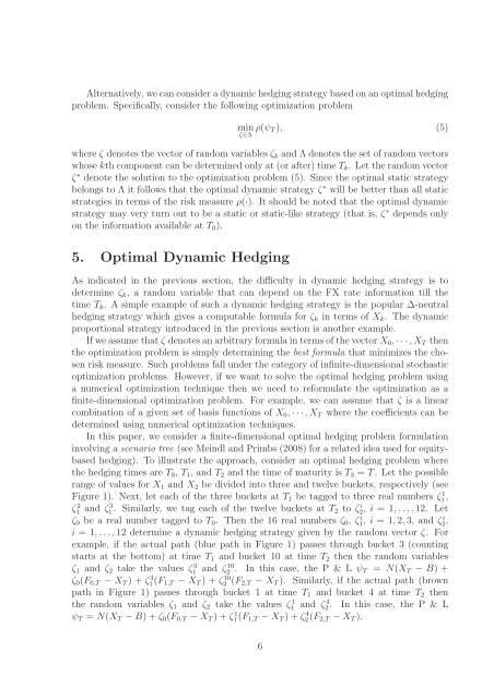
Alternatively, wecanconsideradynamichedgingstrategybasedonanoptimalhedgingproblem. Specifically, consider the following optimization problemmin ρ(ψ T), (5)ζ∈Λwhere ζ denotes thevector ofrandom variablesζ k andΛdenotes the set ofrandomvectorswhose kthcomponent canbedetermined onlyat(orafter)timeT k . Let therandomvectorζ ∗ denote the solution to the optimization problem (5). Since the optimal static strategybelongs to Λ it follows that the optimal dynamic strategy ζ ∗ will be better than all staticstrategies in terms of the risk measure ρ(·). It should be noted that the optimal dynamicstrategy may very turn out to be a static or static-like strategy (that is, ζ ∗ depends onlyon the information available at T 0 ).5. Optimal Dynamic HedgingAs indicated in the previous section, the difficulty in dynamic hedging strategy is todetermine ζ k , a random variable that can depend on the FX rate information till thetime T k . A simple example of such a dynamic hedging strategy is the popular ∆-neutralhedging strategy which gives a computable formula for ζ k in terms of X k . The dynamicproportional strategy introduced in the previous section is another example.Ifweassumethatζ denotesanarbitraryformulaintermsofthevectorX 0 ,···,X T thenthe optimization problem is simply determining the best formula that minimizes the chosenrisk measure. Such problems fall under the category of infinite-dimensional stochasticoptimization problems. However, if we want to solve the optimal hedging problem usinga numerical optimization technique then we need to reformulate the optimization as afinite-dimensional optimization problem. For example, we can assume that ζ is a linearcombination of a given set of basis functions of X 0 ,···,X T where the coefficients can bedetermined using numerical optimization techniques.In this paper, we consider a finite-dimensional optimal hedging problem formulationinvolving a scenario tree (see Meindl and Primbs (2008) for a related idea used for equitybasedhedging). To illustrate the approach, consider an optimal hedging problem wherethe hedging times are T 0 , T 1 , and T 2 and the time of maturity is T 3 = T. Let the possiblerange of values for X 1 and X 2 be divided into three and twelve buckets, respectively (seeFigure 1). Next, let each of the three buckets at T 1 be tagged to three real numbers ζ1 1,ζ1 2 and ζ3 1 . Similarly, we tag each of the twelve buckets at T 2 to ζ2 i , i = 1,...,12. Letζ 0 be a real number tagged to T 0 . Then the 16 real numbers ζ 0 , ζ1, i i = 1,2,3, and ζ2,ii = 1,...,12 determine a dynamic hedging strategy given by the random vector ζ. Forexample, if the actual path (blue path in Figure 1) passes through bucket 3 (countingstarts at the bottom) at time T 1 and bucket 10 at time T 2 then the random variablesζ 1 and ζ 2 take the values ζ1 3 and ζ10 2 . In this case, the P & L ψ T = N(X T − B) +ζ 0 (F 0,T − X T ) + ζ1(F 3 1,T − X T ) + ζ2 10 (F 2,T − X T ). Similarly, if the actual path (brownpath in Figure 1) passes through bucket 1 at time T 1 and bucket 4 at time T 2 thenthe random variables ζ 1 and ζ 2 take the values ζ1 1 and ζ4 2 . In this case, the P & Lψ T = N(X T −B)+ζ 0 (F 0,T −X T )+ζ1(F 1 1,T −X T )+ζ2(F 4 2,T −X T ).6