Simulation of Multiple Line Rail Sections - IEOR @IIT Bombay ...
Simulation of Multiple Line Rail Sections - IEOR @IIT Bombay ...
Simulation of Multiple Line Rail Sections - IEOR @IIT Bombay ...

You also want an ePaper? Increase the reach of your titles
YUMPU automatically turns print PDFs into web optimized ePapers that Google loves.
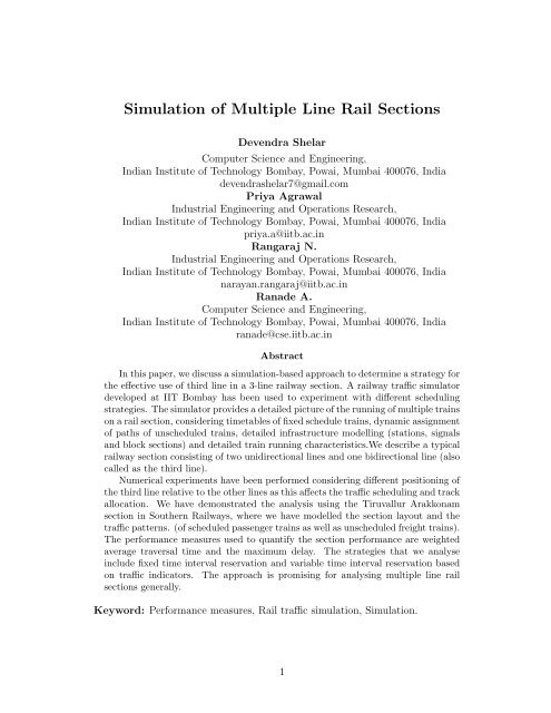
<strong>Simulation</strong> <strong>of</strong> <strong>Multiple</strong> <strong>Line</strong> <strong>Rail</strong> <strong>Sections</strong><br />
Devendra Shelar<br />
Computer Science and Engineering,<br />
Indian Institute <strong>of</strong> Technology <strong>Bombay</strong>, Powai, Mumbai 400076, India<br />
devendrashelar7@gmail.com<br />
Priya Agrawal<br />
Industrial Engineering and Operations Research,<br />
Indian Institute <strong>of</strong> Technology <strong>Bombay</strong>, Powai, Mumbai 400076, India<br />
priya.a@iitb.ac.in<br />
Rangaraj N.<br />
Industrial Engineering and Operations Research,<br />
Indian Institute <strong>of</strong> Technology <strong>Bombay</strong>, Powai, Mumbai 400076, India<br />
narayan.rangaraj@iitb.ac.in<br />
Ranade A.<br />
Computer Science and Engineering,<br />
Indian Institute <strong>of</strong> Technology <strong>Bombay</strong>, Powai, Mumbai 400076, India<br />
ranade@cse.iitb.ac.in<br />
Abstract<br />
In this paper, we discuss a simulation-based approach to determine a strategy for<br />
the effective use <strong>of</strong> third line in a 3-line railway section. A railway traffic simulator<br />
developed at IIT <strong>Bombay</strong> has been used to experiment with different scheduling<br />
strategies. The simulator provides a detailed picture <strong>of</strong> the running <strong>of</strong> multiple trains<br />
on a rail section, considering timetables <strong>of</strong> fixed schedule trains, dynamic assignment<br />
<strong>of</strong> paths <strong>of</strong> unscheduled trains, detailed infrastructure modelling (stations, signals<br />
and block sections) and detailed train running characteristics.We describe a typical<br />
railway section consisting <strong>of</strong> two unidirectional lines and one bidirectional line (also<br />
called as the third line).<br />
Numerical experiments have been performed considering different positioning <strong>of</strong><br />
the third line relative to the other lines as this affects the traffic scheduling and track<br />
allocation. We have demonstrated the analysis using the Tiruvallur Arakkonam<br />
section in Southern <strong>Rail</strong>ways, where we have modelled the section layout and the<br />
traffic patterns. (<strong>of</strong> scheduled passenger trains as well as unscheduled freight trains).<br />
The performance measures used to quantify the section performance are weighted<br />
average traversal time and the maximum delay. The strategies that we analyse<br />
include fixed time interval reservation and variable time interval reservation based<br />
on traffic indicators. The approach is promising for analysing multiple line rail<br />
sections generally.<br />
Keyword: Performance measures, <strong>Rail</strong> traffic simulation, <strong>Simulation</strong>.<br />
1
ISCI 2012 2<br />
1 Introduction<br />
Indian <strong>Rail</strong>ways has a very wide and complex network and variety <strong>of</strong> routes across India.<br />
Across various regions, across various sections the Indian <strong>Rail</strong>ways comprise <strong>of</strong> single<br />
lines, double lines or more than two lines. In certain suburban networks there are also<br />
six parallel tracks set up. There are various performance measures that can be studied to<br />
analyse the track behaviour on a particular section. One can measure throughput (number<br />
<strong>of</strong> trains traversing the section per unit time), headway, average traversal time, maximum<br />
delay for a train etc. However, the sections comprising <strong>of</strong> three lines is <strong>of</strong> peculiar interest<br />
to this particular study. The three-line section comprises <strong>of</strong> two dedicated railway lines.<br />
one reserved for up direction and other for down direction. The third line can be used<br />
in both the direction. The question we will try to address is how a section controller<br />
can utilize the third line for better performance <strong>of</strong> the section across various performance<br />
measures.<br />
As said above, in three-line sections, the third line can be used in both directions as<br />
opposed to the two main lines which can be used only in one direction each. Further, in<br />
a general section, the third line can be in the middle or one <strong>of</strong> the main lines can be in<br />
the middle. The purpose <strong>of</strong> study is to determine in what direction the third line be used<br />
given the traffic parameters in both the directions and the network configuration for the<br />
section. In particular, we will be analysing the performance <strong>of</strong> a Tiruvallur-Arakkonam<br />
section (abbreviated as TRL-AJJ section) in Southern <strong>Rail</strong>ways.<br />
It is observed that during some intervals <strong>of</strong> time the train traffic is more in one direction<br />
than the other direction and during the other intervals <strong>of</strong> time it is vice versa. Hence,<br />
intuition suggests that the direction <strong>of</strong> the third line should be same as the direction in<br />
which there is more train traffic. We identified some ways as how to use the third line.<br />
We tried to determine the direction in which the third line needs to be used during the<br />
various intervals <strong>of</strong> time so as to reduce the overall delay <strong>of</strong> trains. Scheduling strategies<br />
for effective use <strong>of</strong> the third line were discussed.<br />
We have used simulator developed by IIT <strong>Bombay</strong>. It was initially developed for<br />
IRISET (Indian <strong>Rail</strong>ways Institute <strong>of</strong> Signal Engineering and Telecommunication) that<br />
handles train scheduling on a linear section. The simulator finds out a conflict free, feasible<br />
schedule. The simulator also generates a velocity pr<strong>of</strong>ile for the trains using which we can<br />
determine the location and velocity <strong>of</strong> the train at the given time. It handles two kinds <strong>of</strong><br />
trains. scheduled and freight (unscheduled) trains. The loop allocation and the schedule<br />
<strong>of</strong> the freight train can be obtained given the source and the destination station and the<br />
departure time from the source station. The trains are scheduled as per their priorities<br />
and first come first serve criteria. The express trains have the highest priority while the<br />
freight trains have the lowest priority. The current work also aims to see whether this can<br />
be used for larger parts <strong>of</strong> the rail network, by using a combination <strong>of</strong> global and local<br />
scheduling principles.<br />
2 Literature Review<br />
Rangaraj et. al. (2003) have given the detailed description <strong>of</strong> the simulator that we have<br />
used for our experiments. The input and files are described and the algorithm used for<br />
scheduling is described in detail. Abril et. al. (2007) have discussed some techniques for<br />
railway capacity analysis and a simulation based tool, MOM, to perform the same. The
ISCI 2012 3<br />
parameters used are new or existing lines, train mix, regular time tables, traffic peaking<br />
factor, priority, track interruptions, train stop time, maximum trip time threshold, time<br />
window and quality <strong>of</strong> service, reliability or robustness. They have defined capacity as<br />
the ratio <strong>of</strong> time period and headway. Barber et. al. (2008), have discussed simulation<br />
approach for robust timetabling. <strong>Simulation</strong> disruption is performed and the conflicts are<br />
resolved using it. These methods are used in MOM. Homer et. al. (1999), have discussed<br />
strategic planning model for railway system. It evaluates On-Time performance measurement<br />
for freight cars at ultimate destination. Fadadu (2010), in his report has analysed<br />
investment to construct by-pass at a junction, which is a bottleneck in a considered part<br />
<strong>of</strong> the network. The simulator developed by IIT <strong>Bombay</strong> is also used in this. Construction<br />
<strong>of</strong> by-pass or a flyover is suggested based on the analysis <strong>of</strong> the traffic patterns. Raghuram<br />
and Rao (1991) have described experiment design and implementation for line capacity<br />
planning <strong>of</strong> a section <strong>of</strong> running freight trains. The effects <strong>of</strong> variation in the number <strong>of</strong><br />
tracks, signalling mechanism, train speed and starting times for trains have been analysed.<br />
3 Problem Description<br />
3.1 Objective<br />
The main objective <strong>of</strong> the study is to propose a scheme for operating the third line<br />
in the Tiruvallur-Arakkonam section. These stations are abbreviated as TRL and AJJ<br />
respectively. The down direction <strong>of</strong> the section is from TRL to AJJ or the up direction<br />
is from AJJ to TRL direction. The TRL-AJJ section consists <strong>of</strong> 3-railway lines namely<br />
the up main line, down main line and a 3 rd line which can be used in both the directions.<br />
We need to determine how to operate the 3 rd line so that the capacity <strong>of</strong> the section can<br />
be optimally used. An indirect, but useful measure <strong>of</strong> performance in this context is the<br />
average traversal time for trains using the section.<br />
3.2 Description <strong>of</strong> Section<br />
The particular TRL-AJJ section has the up line in the middle. The principle which we<br />
attempt to discuss here can be extended to similar sections anywhere. These sections<br />
could have the 3 rd line in the middle or the down line in the middle. In TRL-AJJ section<br />
there are two main intermediate stations Kadambattur and Tiruvalangadu (abbreviated<br />
as KBT and TI respectively). There are other intermediate stations at which only the<br />
local trains halt. Also, these stations have only as many loops as the number <strong>of</strong> railway<br />
lines, namely 3. At the stations KBT and TL, there are 5 loop lines, each. Hence, there<br />
is scope for change <strong>of</strong> railway tracks by trains and overtaking etc. at these stations. The<br />
following diagram shows the line arrangement at the TRL- AJJ section.<br />
4 Input Modelling<br />
The traffic patterns that are given to the simulator can be specified in various types. It<br />
can either be regular traffic pattern or irregular traffic pattern.
ISCI 2012 4<br />
4.1 Regular traffic<br />
Figure 1: <strong>Line</strong> arrangement <strong>of</strong> TRL-AJJ section<br />
In this type the arrival and departure time for every train is specified at each station. But<br />
delay might occur because <strong>of</strong> various reasons like maintenance <strong>of</strong> tracks, engine failure or<br />
climatic conditions. While simulation, external delays can be added and analysed as part<br />
<strong>of</strong> the future work.<br />
4.2 Irregular traffic<br />
The traffic pattern <strong>of</strong> unscheduled trains is said to be irregular. Some <strong>of</strong> the variations<br />
are listed below:<br />
• The departure times <strong>of</strong> the unscheduled trains from the source station can be determined<br />
based on a fixed headway or a variable headway. Both <strong>of</strong> these strategies<br />
are discussed further in section 6<br />
• We can analyse past traffic for a particular period and fit a theoretical probability<br />
distribution to it.<br />
• The departure times <strong>of</strong> trains can be based on the values obtained from a random<br />
number generator.<br />
• Based on the current trends <strong>of</strong> traffic, the future traffic i. e. the approximate<br />
number <strong>of</strong> trains can be predicted and simulation can be done for the it.<br />
• The speed, acceleration, deceleration <strong>of</strong> the train can be varied.<br />
In this paper we have experimented for the change in headway <strong>of</strong> freight trains and<br />
the real sample data. The analysis <strong>of</strong> the remaining strategies is part <strong>of</strong> our future<br />
work.
ISCI 2012 5<br />
5 Strategies Used<br />
5.1 Nature <strong>of</strong> suggested policy<br />
Let us first define a set <strong>of</strong> parameters to measure the performance <strong>of</strong> the section. Let the<br />
measure <strong>of</strong> traffic in the up direction be Nu and that in the down direction be Nd which<br />
captures the intensity <strong>of</strong> traffic and usage in each direction over a certain time horizon.<br />
5.2 Traffic indicators<br />
The traffic indicators Nu and Nd are computed as follows. Determine a time horizon T<br />
(e.g. two hours) from current time.<br />
• Definition 1: Nu is the weighted sum <strong>of</strong> trains in the up direction that are in the<br />
section or will be in the section during the time interval [0,T ]. The current time is<br />
0.<br />
• Definition 2: Nd is the weighted sum <strong>of</strong> trains in the down direction that are in the<br />
section or will be in the section during the time interval [0,T ]. The current time is<br />
0.<br />
• Definition 3: K is the measure <strong>of</strong> threshold difference between the up-traffic and<br />
down-traffic that would suggest sufficient directional dominance in the down direction.<br />
• Definition 4: L is the measure <strong>of</strong> threshold difference between the up-traffic and<br />
down-traffic that would suggest sufficient directional dominance in the up direction.<br />
We now put down the following aims that we would like to prove by simulation <strong>of</strong> the<br />
TRL-AJJ section with the help <strong>of</strong> the simulator.<br />
• If the third line is currently operating in up direction, change over to down IF<br />
Nd − Nu = K (i.e. continue in up direction if Nd − Nu < K)<br />
• If the third line is currently operating in down direction, change over to up IF<br />
Nu − Nd = L (i.e. continue in down direction if Nu − Nd < L).<br />
In other words, move to a different regime if there is sufficient directional dominance<br />
<strong>of</strong> traffic. The parameters K and L and the method <strong>of</strong> computation <strong>of</strong> the traffic indicators<br />
Nu and Nd will be described below. Let the up trains considered for scheduling<br />
be u1, u2; ...; um with priorities pu1; pu2; ...; pum. Also, let the down trains considered for<br />
scheduling be d1; d2; ...; dn with priorities pd1; pd2; ...; pdn.<br />
• The traffic measure Nu in the up direction is given by:<br />
Nu = pu1 + pu2 + ... + pum<br />
m<br />
• The traffic measure Nd in the down direction is given by:<br />
Nd = pd1 + pd2 + ... + pdn<br />
n<br />
Now, let us define the traversal time <strong>of</strong> a train. A train once into the section <strong>of</strong> interest<br />
can either halt at an intermediate station which is the train’s destination station or exit<br />
the section completely. Therefore, the traversal time <strong>of</strong> the train is defined either to be<br />
the time taken for train to halt at its destination station in the section (if any) or the<br />
time taken by train to exit the section completely adhering to the schedule specified by<br />
the simulator, since its arrival into the section. For e.g. if a train tr enters the station<br />
(1)<br />
(2)
ISCI 2012 6<br />
at time ta and halts at its destination station or exits the section at time te then the<br />
traversal time ttr for train is:<br />
ttr = te − ta<br />
We can further define a weighted average traversal time for all the trains considering<br />
the specific time window. Let’s say that tru1; tru2; ...; trum be the traversal times for the<br />
up trains and trd1; trd2; ...; trdn be the traversal times for the down trains. The priorities<br />
<strong>of</strong> the trains are mentioned earlier. Then the weighted average traversal time for these<br />
trains is defined as:<br />
W AT T =<br />
�m i=1 pui ∗ trui + �n pdi i=1 ∗ trdi<br />
m + n<br />
Given a general scenario, the average traversal time when the 3 rd line is used only in<br />
the up direction and when it is used only in the down direction are bound to be different.<br />
Let us call these times as W AT Tu and W AT Td respectively. On the basis <strong>of</strong> the average<br />
traversal times W AT Tu and W AT Td we compute the values <strong>of</strong> K and L as shown below.<br />
These definitions <strong>of</strong> K and L are specific only for 3-line sections which have the up line<br />
in the middle.<br />
There are two major cases based upon the values <strong>of</strong> Nu and Nd.<br />
• Nu ≥ Nd : In this case, we claim that W AT Tu > W AT Td as shall be shown in the<br />
results <strong>of</strong> the experiment later.<br />
• Nu < Nd : In this case, there are two sub cases:<br />
– W AT Tu > W AT Td: This would be the case when Nu is not much less than<br />
Nd.<br />
Then, let<br />
– W AT Tu ≤ W AT Td: This would be the case when Nu is much less than Nd.<br />
K ′ = Nd − Nu<br />
The smallest such value <strong>of</strong> K ′ is K. Mathematically defined as<br />
K = {minNd − Nu|W AT Tu ≤ W AT Td} (6)<br />
L is defined similarly.<br />
When the difference between the traffic measures Nd - Nu becomes as greater than or<br />
equal to K we will want to change the direction <strong>of</strong> the 3 rd from up to down. However,<br />
once the traffic sets in the section and direction <strong>of</strong> 3 rd line is in down direction, if Nu<br />
which is initially less than Nd, gradually becomes greater than Nd, because <strong>of</strong> existing<br />
traffic changing the direction <strong>of</strong> 3 rd line may not reduce the W AT T . Hence, we change the<br />
direction <strong>of</strong> 3 rd line only when the difference Nu − Nd becomes greater than the threshold<br />
L. i.e. when Nu - Nd > L, change the direction <strong>of</strong> the line from down direction to up<br />
direction to reduce W AT T .<br />
Some claims about the values <strong>of</strong> K and L can be made as follows:<br />
• If the third line is in the middle, we would expect K = L<br />
• If the up line is in the middle, we would expect K > L<br />
• If the down line is in the middle, we would expect K < L<br />
(3)<br />
(4)<br />
(5)
ISCI 2012 7<br />
6 Suggested Control Policy<br />
6.1 Fixed time strategy<br />
6.1.1 Varying the headway <strong>of</strong> freight trains<br />
The indicative values <strong>of</strong> K and L (and T ) are suggested through a simulation exercise<br />
on the TRL - AJJ section. The time window for the experiment was taken to be one<br />
hour. We scheduled 4 down passenger trains each with priority 4 for the experiment. We<br />
vary the parameters u (upHeadway in minutes) and d (downHeadway in minutes) for the<br />
freight trains which are <strong>of</strong> priority 8 each. The priorities are defined on scale 1-10. We<br />
normalize the priorities by dividing it by 11 which is maxP riority + 1. The freight trains<br />
start coming into the section since the beginning <strong>of</strong> the time window at a regular interval<br />
<strong>of</strong> headways. That is the first freight trains in both directions reach the beginning <strong>of</strong> the<br />
section at 0000 hrs. Since the time window is <strong>of</strong> duration 1 hour, the number <strong>of</strong> trains<br />
fired in up direction and down direction are given by nu and nd as follows:<br />
nu =<br />
60<br />
upHeadway<br />
60<br />
nd =<br />
downHeadway<br />
Further the weighted traffic in up direction and down direction will be as follows:<br />
Nu = nu ∗ 8<br />
11<br />
(10)<br />
11<br />
Similarly, the weighted average travelling time (WATT) is obtained.<br />
In this strategy, the time window for experiments was taken 1 hour. The values K<br />
and L would vary depending upon the position <strong>of</strong> the 3rd line with respect to the up main<br />
line and the down main line.<br />
• If the third line is in the middle, we would expect K = L<br />
• If the up line is in the middle, we would expect K > L<br />
• If the down line is in the middle, we would expect K < L<br />
Nd = nd ∗ 8 + 4 ∗ 4<br />
6.1.2 Scheduling as per sample operating data<br />
Some sample operating data covering 8 days was available for the TRL-AJJ section. A<br />
part <strong>of</strong> this data(24 hours duration) is used as the representative data. The assumptions<br />
made about operating practices for this particular are as follows(the details could vary<br />
from section to section in practice):<br />
• The 3 rd line is not used by suburban trains because for this section, because for this<br />
section, the platforms are not available for on the third line at every station. Hence,<br />
the long distance trains which do not halt at the intermediate stations use this line.<br />
• For the up long distance trains the 3 rd line is if higher priority than the UP line<br />
whereas for the down long distance trains the down line is <strong>of</strong> higher priority.<br />
The 3 rd line is reserved in a particular direction for a fixed time interval. The time<br />
interval can typically range from 2 hours to 12 hours. The experimental results have been<br />
shown in section 7.1.2.<br />
(7)<br />
(8)<br />
(9)
ISCI 2012 8<br />
Table 1: Fixed time strategy results<br />
up Headway down Headway Nu Nd W AT Tu W AT Td Direction <strong>of</strong> 3 rd line<br />
5 5 3.270 5.810 17.403 19.482 up<br />
5 6 3.270 5.273 16.132 18.366 up<br />
6 5 2.727 5.810 17.570 18.442 up<br />
7 5 2.455 5.810 17.948 17.820 down<br />
8 5 2.182 5.810 18.023 17.440 down<br />
9 5 1.909 5.810 18.075 17.221 down<br />
9 8 1.909 4.727 15.000 15.011 up<br />
10 13 1.636 3.909 13.201 13.123 down<br />
10 14 1.636 3.909 13.023 12.921 down<br />
11 7 1.636 5.000 15.590 15.385 down<br />
12 10 1.360 4.180 14.123 14.027 down<br />
13 12 1.360 3.909 13.626 13.508 down<br />
14 13 1.360 3.909 13.428 13.147 down<br />
15 16 1.091 3.636 13.367 13.367 -<br />
16 15 1.091 3.636 13.510 13.266 down<br />
6.2 Variable time<br />
In this strategy, the traffic intensity is calculated every hour. If the traffic intensity is<br />
more than the calculated K and L values(as described in section 6.1) then the direction<br />
<strong>of</strong> the third line is changed. The underlying assumptions are same as discussed in section<br />
6.1.2. The experimental results for this strategy have been discussed in section 7.2.<br />
7 Experimental Results<br />
7.1 Fixed time strategy<br />
7.1.1 Varying the headway <strong>of</strong> freight trains<br />
The approach used in the experiments related to table 1 is that, if for certain period <strong>of</strong><br />
time we find the up traffic heavier than the down traffic above a threshold, we dynamically<br />
change the direction <strong>of</strong> the third line from down to up direction (if required). That is we<br />
keep monitoring the values for the traffic and determine the direction <strong>of</strong> the third line.<br />
(The values obtained in Table 1 are as per the calculations shown in section 6.1.1)<br />
The static allocation <strong>of</strong> direction for third line, we do a pre-analysis <strong>of</strong> traffic and fix<br />
a schedule for the third line. Say for example, for half an hour the third line is in up<br />
direction followed by half an hour for which the third line is in down direction, followed<br />
by one hour for which third line can be used in both the directions.<br />
Unscheduled trains are fired for an interval <strong>of</strong> 1 hour. We can see that the direction<br />
<strong>of</strong> the third line is changed when the difference between the traffic measures Nd - Nu<br />
becomes as greater than or equal to K we will want to change the direction <strong>of</strong> the 3 rd<br />
from up to down.<br />
In the table 1 we have not specified the results for all the up headways and down<br />
headways.This is because, as the down head way increases, or the down traffic decreases,<br />
the usage <strong>of</strong> third line changes from down direction to up direction. However, if we reach<br />
a stage where W AT Tu and W AT Td both are equal, that means even if we further reduce
ISCI 2012 9<br />
Table 2: Fixed strategy results for real data<br />
Time slots Nu Nd W AT Tu W AT Td Direction <strong>of</strong> 3 rd line<br />
0-6 7.727 3.818 13.032 16.799 up<br />
6-12 5.727 4.182 8.78 17.671 up<br />
12-18 4.636 8.727 11.801 14.127 up<br />
18-24 5.727 8.818 8.189 11.839 up<br />
Table 3: Variable strategy results for real data<br />
Time slots Nu Nd W AT T Direction <strong>of</strong> 3 rd line (per hour)<br />
0-6 7.727 3.818 13.712 down, down, up, up, up, down<br />
6-12 5.727 4.182 10.760 down, down, up, up, up, up<br />
12-18 4.636 8.727 14.172 down, down, down, down, down, down<br />
18-24 5.727 8.818 10.391 down, up, up, up, up, down<br />
the down traffic, the W AT T values will be the same whether the third line is used in the<br />
up direction or the down direction. The reason behind this is that the traffic in both the<br />
directions is so less in these cases that the third line is not at all used.<br />
7.1.2 Scheduling trains as per the given time table<br />
The time slots considered for these experiments is 6 hours i.e. a set <strong>of</strong> 4 such experiments<br />
over a period <strong>of</strong> 24 hours. The results <strong>of</strong> the same have been shown in table 2. The 3 rd<br />
track is reserved in the up and down direction for all the for sets, W AT Tu and W AT Td<br />
are calculated respectively.<br />
7.2 Variable time strategy<br />
In this section the time slots <strong>of</strong> 6 hours are considered and the direction <strong>of</strong> the 3 r d line<br />
is calculated based on the traffic intensity for each hour. In this case(while calculating<br />
W AT Tu the direction in the respective time slots are:<br />
• {0-1,1-2,2-3,3-4,4-5,5-6} = {down, down, up, up, up, down}<br />
• {6-7, 7-8, 8-9, 9-10, 10-11, 11-12} = {down, down, up, up, up, up}<br />
• {12-13, 13-14, 14-15, 15-16, 16-17, 17-18} = {down, down, down, down, down,<br />
down}<br />
• {18-19, 19-20, 20-21, 21-22, 22-23, 23-24} = {down, up, up, up, up, down}<br />
(The above values are calculated as per the formulae in section 5.2). The directions are<br />
taken opposite while calculating W AT Td. The results are shown in table 3.<br />
We observe from the table 4 that the fixed time strategy shows better results than<br />
the variable time strategy in all the time-slots. The reason is that changing direction <strong>of</strong><br />
the third line causes a certain overhead which results from the flushing out <strong>of</strong> the trains<br />
actually running on the line.<br />
8 Conclusion<br />
The operational strategy for utilizing a resource like the third line in heavy traffic sections<br />
is not obvious. It depends on a number <strong>of</strong> factors like the location <strong>of</strong> the third line with
ISCI 2012 10<br />
Table 4: Comparison <strong>of</strong> variable and fixed time strategies<br />
Time slots Nu Nd F ixedu F ixedd Variable<br />
0-6 7.727 3.818 13.032 16.799 13.712<br />
6-12 5.727 4.182 8.878 17.671 13.544<br />
12-18 4.636 8.727 11.801 14.127 14.172<br />
18-24 5.727 8.818 10.189 11.839 10.391<br />
respect to the other two, the location <strong>of</strong> crossover points, the traffic density, the traffic<br />
mix and finally the performance measures <strong>of</strong> relevance to the rail operator. <strong>Simulation</strong><br />
provides a good means for evaluating different strategies.<br />
In this paper we have reviewed the performance measures like, traffic intensity and<br />
weighted average traversal time which are used as the decision making parameters for the<br />
3 line railway section. <strong>Simulation</strong> also plays a major role in railway scheduling which has<br />
been done using the simulator developed by IIT <strong>Bombay</strong><br />
We experiment with the simple one <strong>of</strong> fixed time regimes and compare it with more<br />
complex strategies like variable time strategy involving some system state measures. More<br />
sophisticated control strategies using long run simulations can also be proposed and evaluated<br />
by other analytical techniques in future. The ones we have suggested have the<br />
advantage <strong>of</strong> being implementable with minimum additional infrastructure and training<br />
<strong>of</strong> personnel involved in the decision.<br />
Based on our experiments we can say that the WATT <strong>of</strong> fixed startegy is less than<br />
variable. More refined results can be obtained by analysing data for a variety <strong>of</strong> traffic<br />
and longer time which is a part <strong>of</strong> our future work.<br />
References<br />
[1] M. Abril, M. Barber, L. Ingolloti, M. A. Salido, P. Tormos, A. Lova A, “An assessment<br />
<strong>of</strong> railway capacity”, Transport. Res. Part E, 2007.<br />
[2] F. Barber, L. Ingolloti, M. A. Salido, “A <strong>Simulation</strong> tool to evaluate the robustness<br />
<strong>of</strong> railway timetables”, PSCS 2008.<br />
[3] Pratik V. Fadadu, “Network Level Investments to Improve <strong>Rail</strong> Capacity”, M.Tech<br />
Project Report, Industrial engineering and Operations Research, IIT <strong>Bombay</strong>, 2011<br />
[4] Jack B. Homer, Thomas E. Keane, Natasha Lukiantseva, David W. Bell, “Evaluating<br />
Strategies to Improve <strong>Rail</strong>road Performance - A System Dynamics Approach”, Winter<br />
<strong>Simulation</strong> conference, 1999<br />
[5] G. Raghuram and V. V. Rao, “A decision support system for improving railway line<br />
capacity”, Public Enterprise,Vol-11(1), pp.64-72 (1991).<br />
[6] N. Rangaraj, A. Ranade, K. Moudgalya, C. Konda, M. Johri and R. Naik “Simulator<br />
for <strong>Line</strong> Capacity Planning”, Sixth Asia Pacific Operations Research Society, Delhi,<br />
December 2003